Scaime eNod3-D User Instructions

Download

Page 1

eeNNoodd33--D

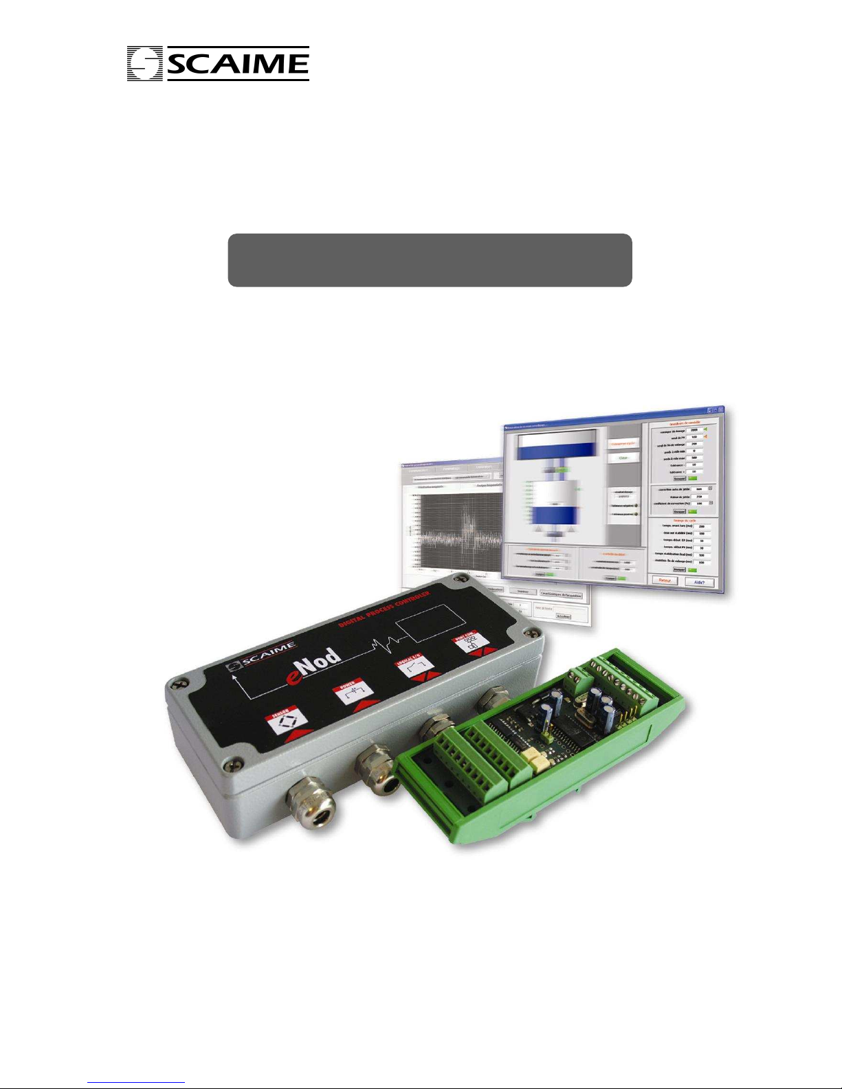
DDiiggiittaall ddoossiinngg ccoonnttrroolllleer

eNod3-D : User’s instructions 165 752-A 1/23

User’s instructions

Page 2

eeNNoodd33--D

DDiiggiittaall ddoossiinngg ccoonnttrroolllleer

eNod3-D : User’s instructions 165 752-A 2/23

1 GENERAL PRESENTATION :..............................................................................4

1.1 Dimensions : ....................................................................................................................................4

1.2 General characteristics :..................................................................................................................5

2 INTERFACES : .....................................................................................................6

2.1 Connection to power supply : ..........................................................................................................6

2.2 Connection to load cell(s) : ..............................................................................................................6

2.3 Connection of inputs and outputs : ..................................................................................................7

2.3.1 Digital inputs...........................................................................................................................7

2.3.2 Digital outputs.........................................................................................................................7

3 COMMUNICATION INTERFACES : .....................................................................8

4 COMMUNICATION :.............................................................................................9

4.1 ModBus RTU : .................................................................................................................................9

4.2 SCMBus :.........................................................................................................................................9

4.2.1 Fast SCMBus format :............................................................................................................9

4.3 CANopen : .......................................................................................................................................9

5 CALIBRATION :..................................................................................................10

5.1 Calibration types :..........................................................................................................................10

5.2 Non-linearity correction..................................................................................................................10

6 INPUTS FUNCTIONING : ...................................................................................11

6.1 Inputs assignement :......................................................................................................................11

6.2 Functions independant of the functioning mode :.......................................................................... 11

6.3 Functions specific to each functioning mode :............................................................................... 11

7 OUTPUTS FUNCTIONING : ...............................................................................12

7.1 Outputs assignement :...................................................................................................................12

7.2 Functions independant of the functioning mode :.......................................................................... 12

7.3 Functions specific to each functioning mode :............................................................................... 12

7.4 Feeding mode in dosing processes............................................................................................... 13

8 SET POINTS :.....................................................................................................13

9 FILTERS : ...........................................................................................................13

10 TRANSMITTER FUNCTIONING MODE : ...........................................................14

10.1 Measurement reading request :.....................................................................................................14

10.1.1 Single measurement transmission :.....................................................................................14

10.1.2 Continuous measurement transmission...............................................................................14

10.2 Specific commands through an input :...........................................................................................14

10.2.1 Transmit measurement (Fig. 4)............................................................................................14

10.2.2 Measurement window (Fig. 5)..............................................................................................15

10.2.3 Clear.....................................................................................................................................15

11 DOSING BY FILLING FUNCTIONING MODE :..................................................16

11.1 Starting conditions .........................................................................................................................17

11.2 Cycle description............................................................................................................................18

11.2.1 Flow rate control (optional)...................................................................................................18

11.2.2 Automatic taring at start .......................................................................................................18

11.2.3 Coarse feed effect neutralization time..................................................................................18

11.2.4 Fine feed level ......................................................................................................................18

11.2.5 Fine feed effect neutralization time......................................................................................18

11.2.6 Target weight and inflight weight..........................................................................................19

11.2.7 Final stabilization time..........................................................................................................19

11.2.8 Tolerances............................................................................................................................19

11.2.9 End of emptying level and emptying holding time................................................................19

11.2.10 End of cycle waiting time......................................................................................................19

11.2.11 Effective end of cycle............................................................................................................19

11.3 Digital inputs utilization ..................................................................................................................19

11.3.1 Start cycle.............................................................................................................................19

11.3.2 Suspend current cycle..........................................................................................................19

11.3.3 Stop cycle.............................................................................................................................20

12 DOSING BY UNLOADING FUNCTIONING MODE : ..........................................20

12.1 Reloading management.................................................................................................................22

Page 3

eeNNoodd33--D

DDiiggiittaall ddoossiinngg ccoonnttrroolllleer

eNod3-D : User’s instructions 165 752-A 3/23

12.1.1

Reloading at the end of the cycle.........................................................................................22

12.1.2 Reloading at the start of the cycle........................................................................................22

12.2 Cycle description............................................................................................................................22

12.2.1 Flow rate control (optional)...................................................................................................22

12.2.2 Verification of the available product quantity........................................................................22

12.2.3 Start delay ............................................................................................................................22

12.2.4 Coarse feed effect neutralization time..................................................................................22

12.2.5 Fine feed level ......................................................................................................................22

12.2.6 Fine feed effect neutralization time......................................................................................22

12.2.7 Target weight and inflight weight..........................................................................................23

12.2.8 Final stabilization time..........................................................................................................23

12.2.9 Tolerances............................................................................................................................23

12.2.10 End of cycle waiting time......................................................................................................23

12.2.11 Effective end of the cycle .....................................................................................................23

12.3 Digital inputs utilization ..................................................................................................................23

12.3.1 Start cycle.............................................................................................................................23

12.3.2 Suspend current cycle..........................................................................................................23

12.3.3 Stop cycle.............................................................................................................................23

Page 4

eeNNoodd33--D

DDiiggiittaall ddoossiinngg ccoonnttrroolllleer

eNod3-D : User’s instructions 165 752-A 4/23

1 GENERAL PRESENTATION :

eNod3-D provides an economic high performance solution to transform any strain gauge sensor into an

intelligent digital system. eNod3-D includes three advanced operating modes for control of static and dynamic processes :

- measurements transmitter

- dosing by filling

- dosing by unloading

eNod3-D is equiped with RS485/422, RS232 and CANbus outputs supporting ModBus-RTU, SCMBus

and CANopen protocols. Each module is also provided with 2 digital inputs and 4 digital outputs, authorizing synchronization of functions with automation and alarm management. SCAIME provides the eNodView software to facilitate installation of eNod3-D to set parameters and calibrate the measurement system, for acquisition of measurements and simulation of digital filters.

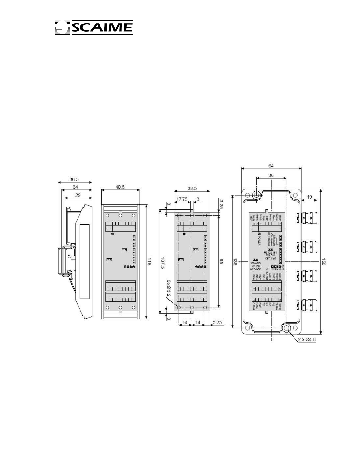
1.1 Dimensions :

Single board card

Waterproof

housing version

DIN rail version

Page 5

eeNNoodd33--D

DDiiggiittaall ddoossiinngg ccoonnttrroolllleer

eNod3-D : User’s instructions 165 752-A 5/23

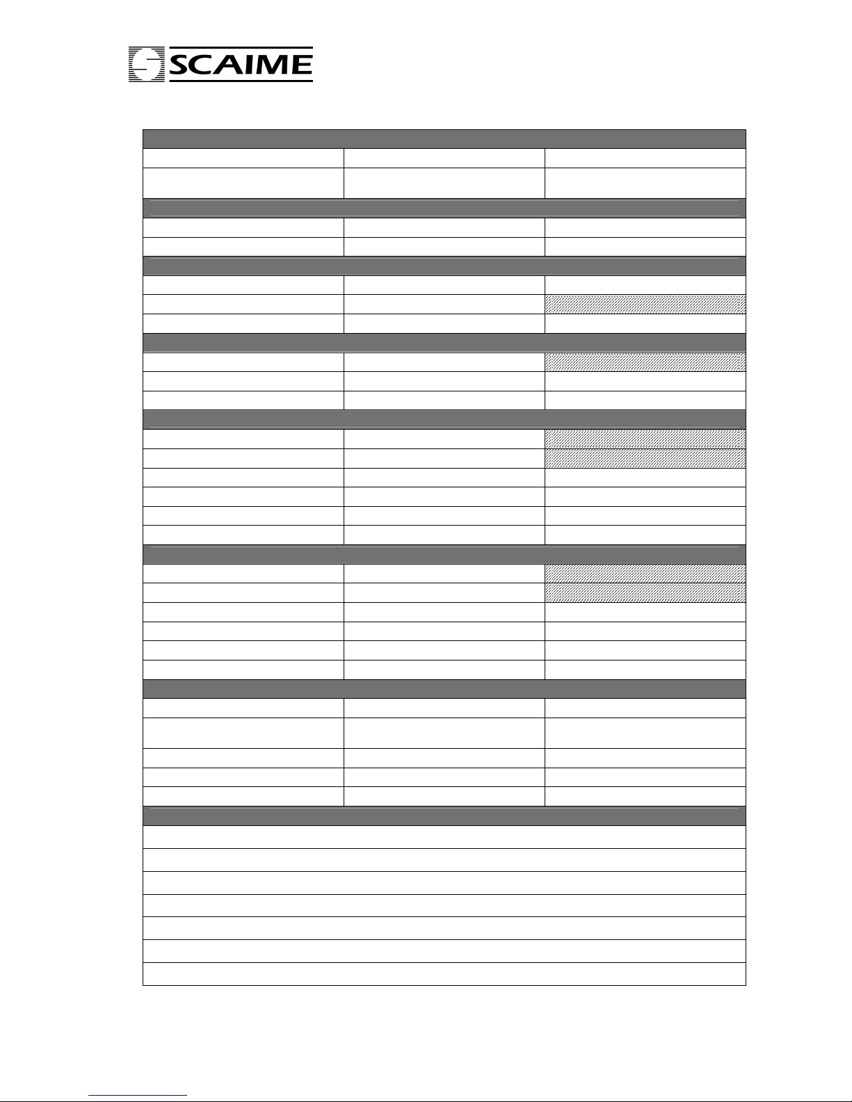
1.2 General characteristics :

Power supply

power supply voltage 10 ..... 28 VDC

max consumption

70 with 350Ω load cell 120 with 80Ω load cell

Temperature range

storage temperature -25...+85 °C

operating temperature -10...+40 °C

Load cell

impedance (complete bridge)

80 Ω

connection 4 or 6 wires

load cell power supply 5 ± 5% VDC

Communication

RS 485/422 and RS232 Half or full-duplex

RS baud rate 9600 ... 115200 bauds

Can 2.0A 20....1000 kbauds

Logical inputs

number 2

type optocoupler

low-level voltage 0 ..... 3 VDC

high-level voltage 9 .... 28 VDC

current at high level 10mA @ 24V mA

insulation voltage 2500 V

rms

Logical outputs

number 4

type opto-insulated static relays

max current @ 40°C 0.4 A

max voltage in open state 55 V

resistance in ON state 2 Ω

insulation voltage 2500 V

rms

Metrological characteristics

analog input signal range 7.8 ... 500 mV/V

typical temperature offset drift

@ input signal range <7,8 mV/V

1.5 ppm/°C

typical slope temperature effect 2 ppm/°C

max linearity error 0.003 %

A/D conversion rate 1920 .... 6.25 meas./s

Programmable functions

acquisition of zero, taring, zero tracking

physical or theoretical calibration

slope correction

non-linearity polynomial correction

low-pass, band-stop and self-adaptive digital filters

set points (up to 4) management

dosing (by filling or by unloading) processes control

Page 6

eeNNoodd33--D

DDiiggiittaall ddoossiinngg ccoonnttrroolllleer

eNod3-D : User’s instructions 165 752-A 6/23

2 INTERFACES :

2.1 Connection to power supply :

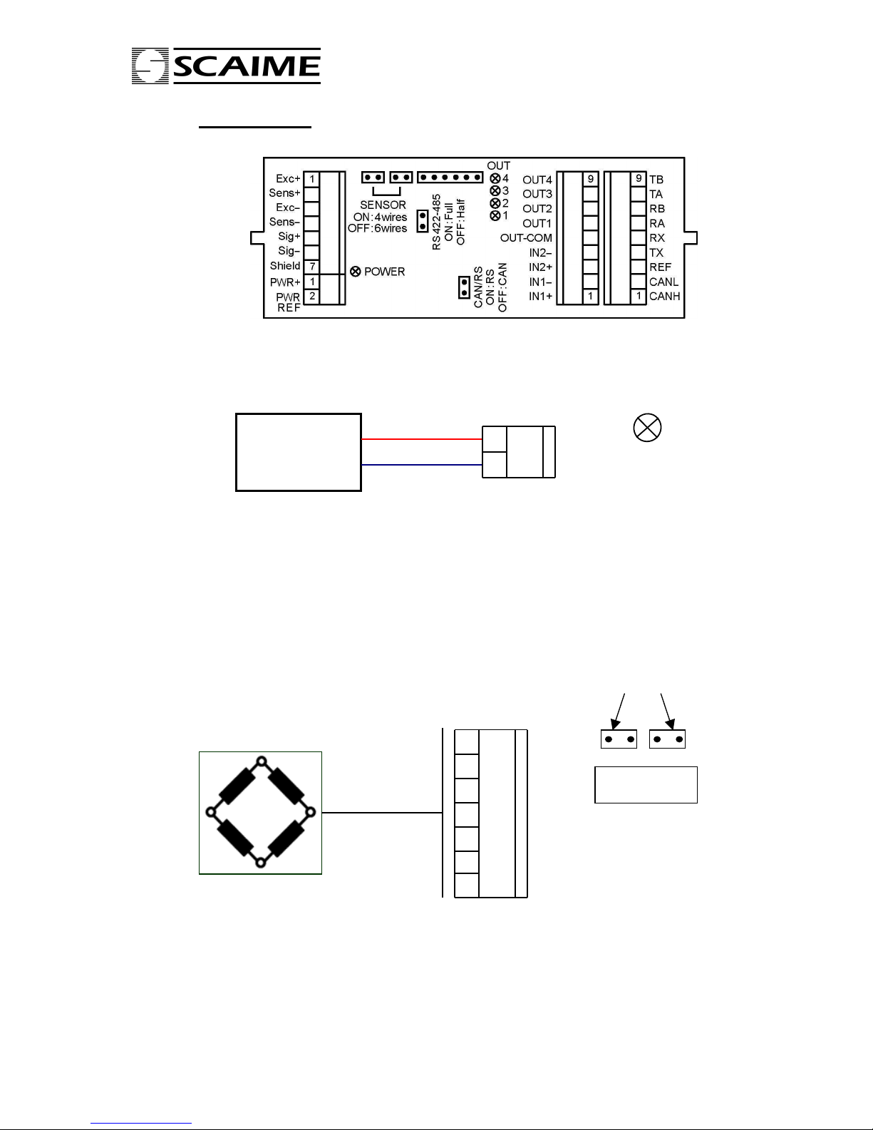
The ‘POWER’ light on the board shows wheter or not the power supply is correctly connected.

2.2 Connection to load cell(s) :

eNod3-D supplies power to the load cells (5 VDC).

Up to four 350Ω load cells can be connected in parallel.

eNod3-D allows the use of 4- or 6- wire load cells.

- 4-wire load cells : jumpers in place

- 6-wire load cells : jumpers removed

Power supply

10 to 28VDC

PWR+

PWR

REF

POWER

4/6- wire jumpers

ON : 4 wires

OFF : 6 wires

Exc+

Sens+ ExcSensSig+ SigShield

1 2 3 4 5

6 7

Page 7

eeNNoodd33--D

DDiiggiittaall ddoossiinngg ccoonnttrroolllleer

eNod3-D : User’s instructions 165 752-A 7/23

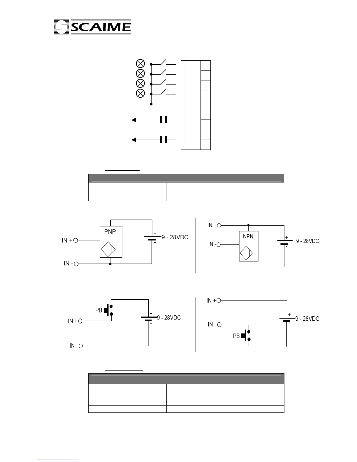
2.3 Connection of inputs and outputs :

2.3.1 Digital inputs

 connection to a detector :

 connection to a push button (PB) :

2.3.2 Digital outputs

Opto-insulated inputs characteristics

high level 9 to 28VDC – Consumption : 10mA @ 24VDC

low level 0 to 3 VDC

Opto-insulated outputs characteristics

max currect @ 40°C 0.4 A max voltage in open state 55 V resistance in the ON state 2 Ω

insulation voltage 2500 V

rms

OUT 4

OUT 3 OUT 2 OUT 1 OUT

COM

IN 2 – IN 2 + IN 1 – IN 1 +

7 6 5 4 3 2

Page 8

eeNNoodd33--D

DDiiggiittaall ddoossiinngg ccoonnttrroolllleer

eNod3-D : User’s instructions 165 752-A 8/23

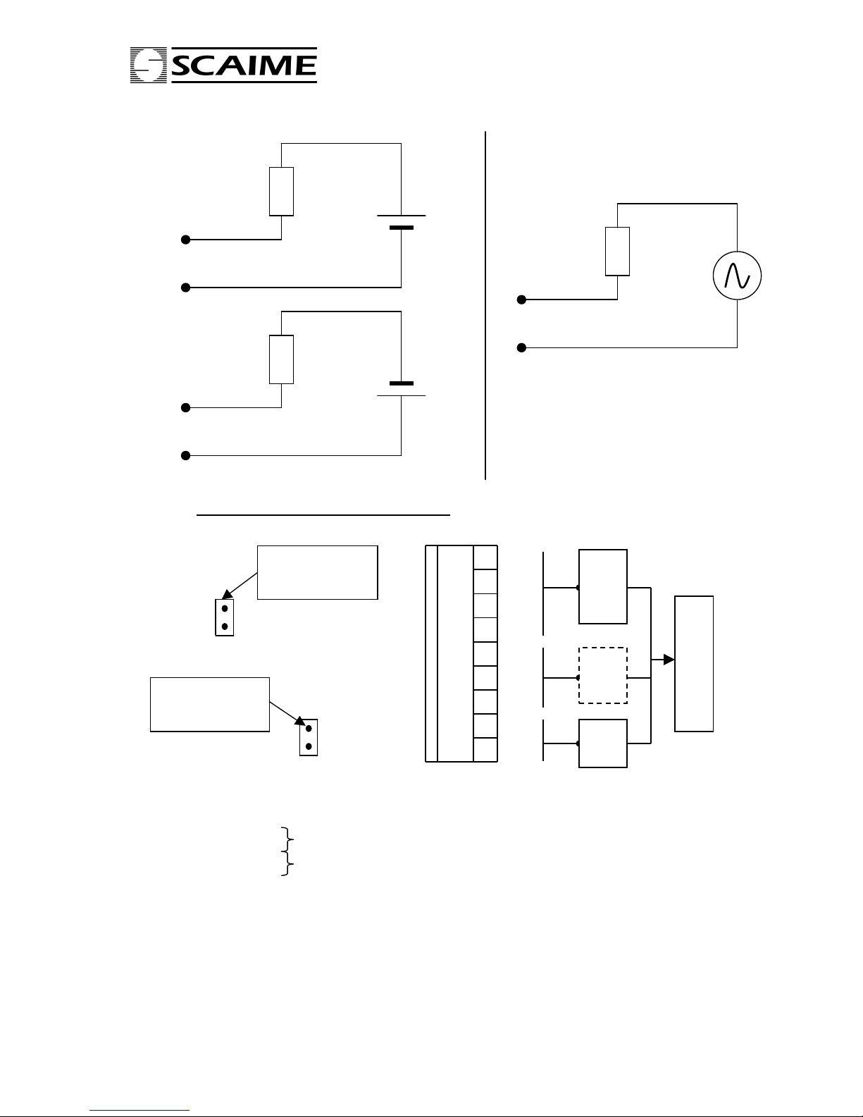
A light is assgined to each output.

3 COMMUNICATION INTERFACES :

eNod3-D is capable of communicating with an automatic control for each connection :

- RS485 / 422

- RS232

- CAN

The connection to the RS 485 / RS 422 interface is made through TA, TB and RA, RB connections on the 9-pins connector. (TA = direct transmission, TB = inverse transmission, RA = direct reception, RB = inverse reception). For an RS485 (half duplex) communication, just connect the TB and TA pins and remove the corresponding jumper (OFF). For an RS422 or RS485 full-duplex communication, use the four TB, TA, RB and RA pins. The corresponding jumper must be in place (ON) (which is the default case on delivery).

The RS232 interface is connected using Tx, Rx and REF connections on the 9-pin connector.

CAN/RS jumper ON CAN/RS jumper OFF

RS485 jumper ON : Full duplex OFF : Half duplex

CAN / RS jumper ON : RS OFF : CAN

TA RB RA Rx TX REF CANL

CANH

RS232

CAN

RS485

Half/Full

communication

7 6 5 4 3 2 1

55 VDC max

OUT

COM

OUT

Load

55 VDC max

OUT

COM

OUT

Load

OUT

COM

OUT

Load

38 VAC max

Page 9

eeNNoodd33--D

DDiiggiittaall ddoossiinngg ccoonnttrroolllleer

eNod3-D : User’s instructions 165 752-A 9/23

The CAN interface is connected using the CANH, CANL and REF (not mandatory) connections on the 9-pin connector.

4 COMMUNICATION :

eNod3-D can communicate using several protocols :

- ModBus RTU

- SCMBus standard format or fast format.

- CANopen

 Switching from the SCMBus protocol to the ModBus-RTU protocol (and reciprocally) can be done

by software programmation.

1) send the corresponding command

2) send the ‘storage in EEPROM’ command

3) reset (hardware or software)the device See example describing how to switch from ModBus-RTU to SCMBus protocol in the document SCMBUS communication Ref 165 756 Appendix A.

 Switching from SCMBus/ModBus-RTU protocol to CANopen protocol (and reciprocally) can be

done by setting or removing the appropriate jumper (cf. §3) then by making a reset

4.1 ModBus RTU :

See the descritption of the different communication frames in the document : ModBus-RTU communication Ref. 165754

4.2 SCMBus :

See the descritption of the different communication frames in the document : SCMBus communication Ref. 165756.

The SCMBus protocol has got similarities with ModBus-TU. It is based on the master/slave structure however it allows to transmit measurements continuously without collision management on the line. This operating mode is only available in transmitter functioning mode. The measurements transmission frequency depends on the serial baud rate thus transmitting 100 meas/s is impossible at less than 19200 bauds. For fast measurement transmissions, use the fast SCMBus format with wich 1200 meas/s can be expected at 115200 bauds.

Other methods of transmitting information without any master request :

- transmitter mode : measurement transmission triggered by a digital input.

- whatever the functioning mode is, physical calibration procedure : automatic transmission when a step in the process is complete.

4.2.1 Fast SCMBus format :

The fast SCMBus format is particularly useful for measurement acquisition at the highest rate, for example in order to analyze dynamic phenomena. This format should only be used for point-to-point opreation in full-duplex. So as to optimize the speed, in addition to using the fast SCMBus format, it is preferable to configure

eNod3-D in ‘non-processing transmitter’. In his operating mode, filters are disabled, set points are not

managed and there is no polynomial linearization.

4.3 CANopen :

eNod3-D supports CANopen communication protocol and is compliant with ‘CiA Draft Standard V301’.

Refer to the decription note : CANopen communication Ref. 165758.

Page 10

eeNNoodd33--D

DDiiggiittaall ddoossiinngg ccoonnttrroolllleer

eNod3-D : User’s instructions 165 752-A 10/23

5 CALIBRATION :

5.1 Calibration types :

There are different possible calibration types (see examples in the documents : communication SCMBus Réf. 165 756’ Appendix A and communication ModBus RTU Réf. 165 754 Appendix A) :

 Physical calibration using known references on the load cell. This type of calibration can be done

with 1, 2 or 3 known loads.

 Theoretical adjustment by setting the load cell sensitivity and a corresponding capacity.  Correction of the initial calibration value with a coefficient.

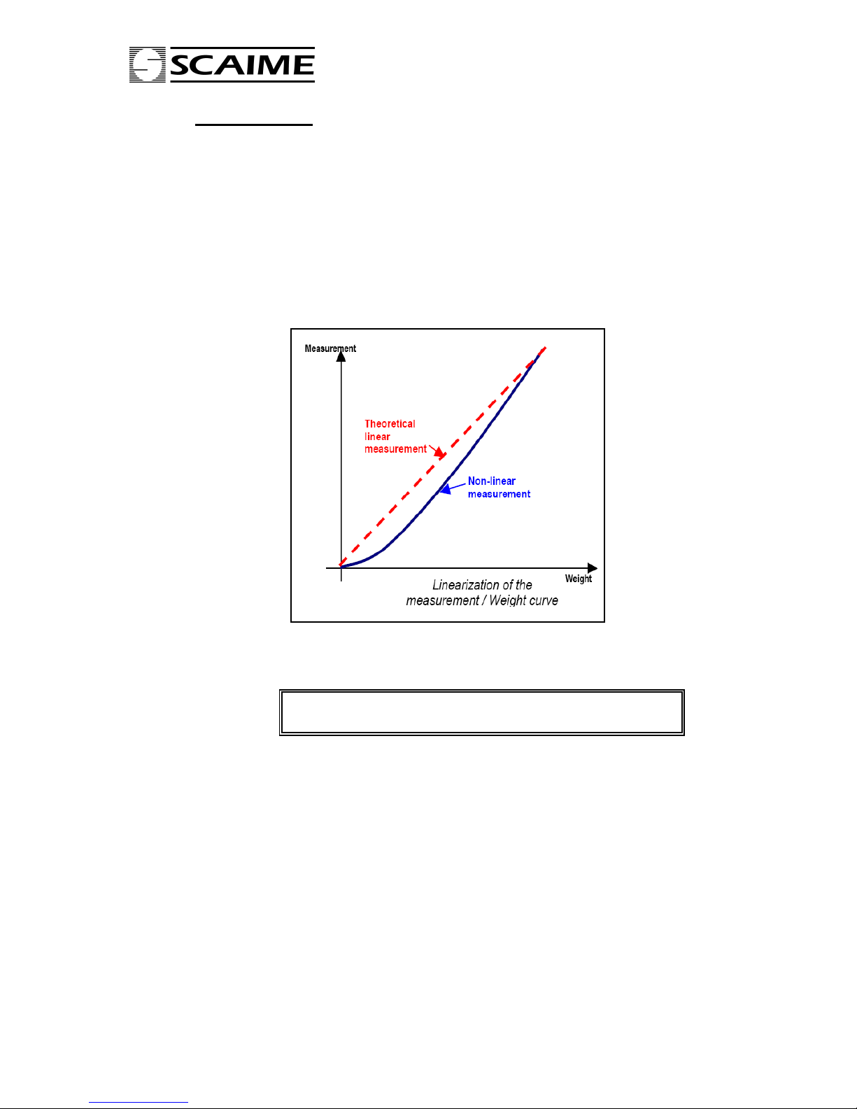
5.2 Non-linearity correction

For an installation with a non-linearity :

The linearization formula is as follows

The three A, B and C coefficients can be determined using eNodView software.

Corrected measurement = Meas – A (Meas)2 – B(Meas) – C where Meas = current measurement

Fig. 1

Page 11

eeNNoodd33--D

DDiiggiittaall ddoossiinngg ccoonnttrroolllleer

eNod3-D : User’s instructions 165 752-A 11/23

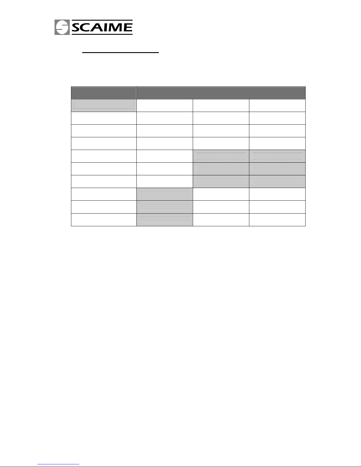
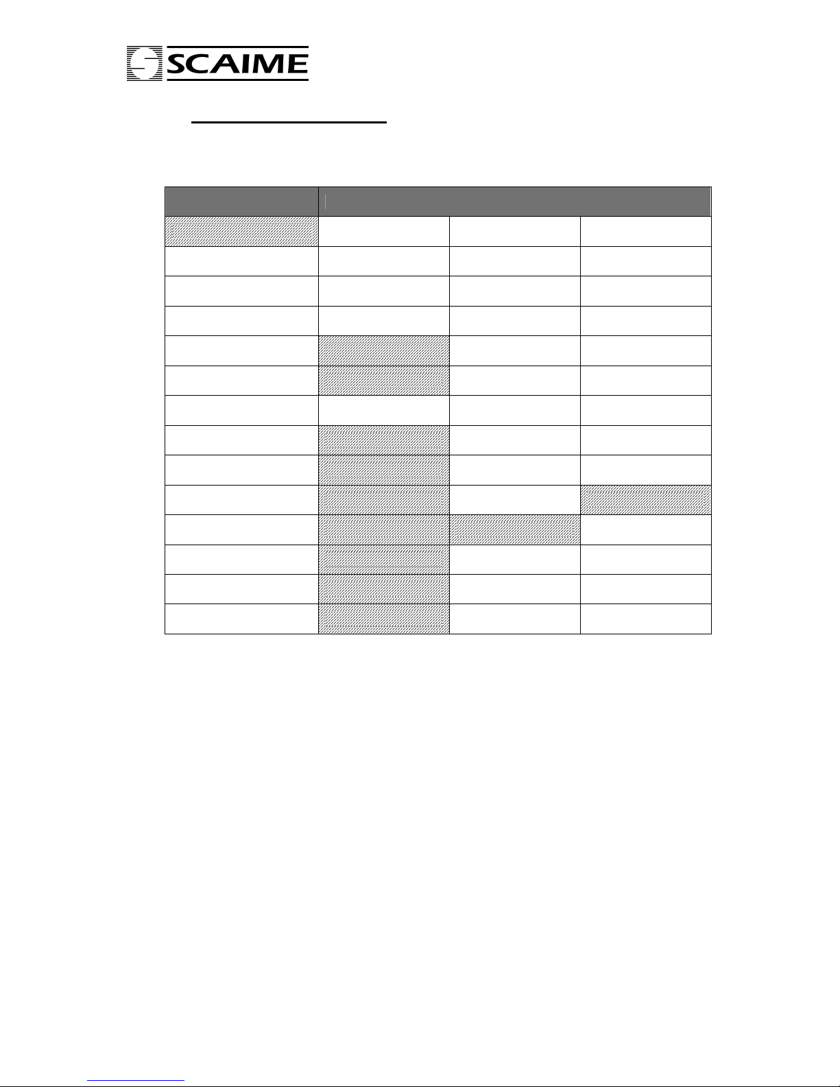
6 INPUTS FUNCTIONING :

Each input can work in positive or negative logic individually. A debounce time attached to both inputs can be adjusted.

6.1 Inputs assignement :

Function Functioning mode

transmitter dosing by filling dosing by unloading

none ● ● ●

tare ● ● ●

zero ● ● ●

transmit measurement ●

measurement window ●

clear ●

start/restart cycle ● ●

stop cycle ● ●

suspend current cycle ● ●

6.2 Functions independant of the functioning mode :

- none : Inputs have no effect.

- tare : one or the other or both inputs can be assigned to the tare function. The tare acquisition is conditioned by a stability criterion that can be changed or inhibited. Depending on the choosen logic (positive or negative), the tare is triggered by a rising or a falling edge.

- zero : one or the other or both inputs can be assigned to the zero function. A new volatile zero value is acquired only if its value is within ±10% range of the specified capacity. The zero acquisition is conditioned by a stability criterion that can be changed or inhibited. Depending on the choosen logic (positive or negative), the tare is triggered by a rising or a falling edge.

6.3 Functions specific to each functioning mode :

See corresponding sections for a complete description.

Page 12

eeNNoodd33--D

DDiiggiittaall ddoossiinngg ccoonnttrroolllleer

eNod3-D : User’s instructions 165 752-A 12/23

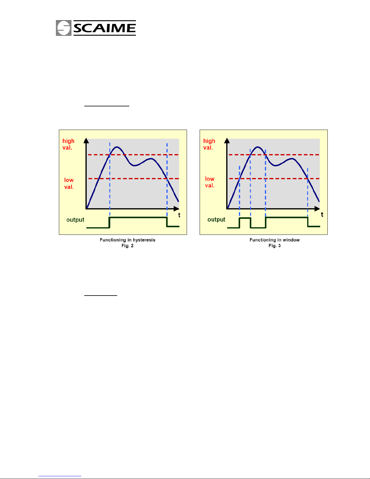
7 OUTPUTS FUNCTIONING :

Each output can work individually in its own logic.

7.1 Outputs assignement :

function Functioning mode

transmitter dosing by filling dosing by unloading

set point ● ● ●

motion ● ● ●

defective measurement ● ● ●

dosing result available

● ●

cycle in progress

● ●

input image ● ● ●

fine feed

● ●

coarse feed ● ●

emptying ●

reloading ●

out of tolerances ● ●

flow rate failure ● ●

dosing failure ● ●

7.2 Functions independant of the functioning mode :

- set point : the outputs can be assigned to configurable set points (cf. §8) Output 1 is assigned to set point 1 , output 2 to set point 2, output 3 to set point 3 and output 4 to set point 4.

- Motion : The outputs can be assigned to copying measurements stability.

- Defective measurement : The outputs can be assigned to copying the measurements faults.These faults are also coded in the status word :

∗ Signal outside the converter analog input range ∗ Signal outside the capacity on the positive side ∗ Signal outside the capacity on the negative side

- Input image : Outputs can be assigned to copying inputs state, either using the same logic or inverting the input state (negative logic). Outputs 1 and 3 are assigned to input 1 and outputs 2 and 4 are assigned to input 2.

7.3 Functions specific to each functioning mode :

See corresponding sections for a complete description.

Page 13

eeNNoodd33--D

DDiiggiittaall ddoossiinngg ccoonnttrroolllleer

eNod3-D : User’s instructions 165 752-A 13/23

7.4 Feeding mode in dosing processes

For the filling and dosing by unloading functioning modes, it is possible to select the activation order of the feed outputs :

 coarse feed then fine feed after coarse feed stop  coarse feed + fine feed at the beginning of the cycle  coarse feed only

8 SET POINTS :

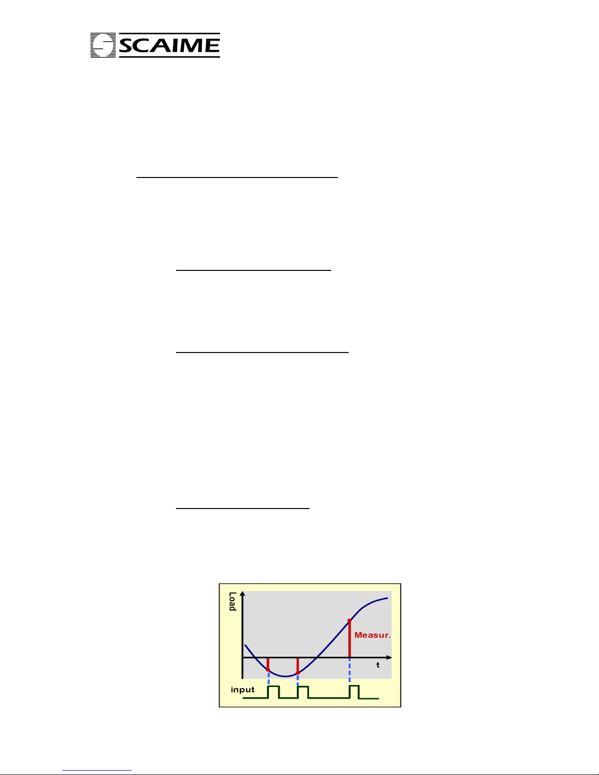
Set points are characterized by a high and a low value. Their operating mode is either operating in hysteresis or operating in window.

The low and high values of these set points may be assigned either to (regardless of the functioning mode) :

- gross measurement

- net measurement

9 FILTERS :

There are four available filtering levels :

∗ filtering related to the A/D conversion rate including rejection of the mains frequency (50 or

60 Hz) harmonics.

∗ 2nd, 3rd or 4th order low-pass Bessel/Butterworth filter ∗ 2nd order band-stop filter ∗ self-adaptive filter

- Filtering related to the A/D conversion rate : the signal resolution is related to the conversion rate. The conversion rate might be choosen as low as possible, particularly for static applications. For dynamic applications, a compromise must be found between the measurement rate and the low-pass filter cut-off frequency. The eNodView software can be used to determine appropriate filter values. Choose a measurement rate that rejects the mains frequency harmonics according to the place of use, 50 or 60Hz.

- Bessel or Butterworth type low pass filter : a low-pass digital filter can be applied as an output of the A/D converter. The filter order is configurable (available values are 2, 3 or 4) and the coefficients that define it depend on the A/D conversion rate, the wanted cutt-off frequency and on the choosen order. These coefficients can be easily calculated by eNodView software.

- Band-stop filter : a 2

order band-stop filter might be applied as an output of the low-pass filter (if

used) or the A/D converter. It allows to attenuate the frequencies within a band defined by a high and a

Page 14

eeNNoodd33--D

DDiiggiittaall ddoossiinngg ccoonnttrroolllleer

eNod3-D : User’s instructions 165 752-A 14/23

low cut-off frequencies. The coefficients that define it depend on the A/D conversion rate and the wanted cutt-off frequencies (that means the frequency band width). These coefficients can be easily calculated by

eNodView software.

- Self-adaptive filter : this filter can be set in cascade after previous filters. It is particularly efficient for static measurements but avoid using it in dynamic or dosing processes. The aim of this filter is to eliminate erratic measurements and to average consistent measurements.

10 TRANSMITTER FUNCTIONING MODE :

This basic functioning mode consists in transmitting measurements on the bus, possibly after configuring them, filtering them and comparing them to set point levels. Measurements can be transmitted individually regardless of the communication protocol or continuously at a defined frequency in SCMBus (standard or fast format) or CANopen protocols. Functioning may be unipolar (positive analog signal only) or bipolar (positive or negative analog signal).

10.1 Measurement reading request :

10.1.1 Single measurement transmission :

Regarless of the communication protocol in use. The request can apply to :

- gross measurement

- net measurement

- tare value

- measurement in A/D converter points

10.1.2 Continuous measurement transmission

This is possible using standard or fast SCMBus format, the transmission can be started by a serial command and another one allows stopping it. Measurements are transmitted at a period defined in ms by the ‘sampling period’ setting. The request can apply to

- gross measurement

- net measurement

- measurement in A/D converter points



Note : This is very similar to operation of ‘Measurement window’ through an input command.

CANopen protocol also allows to define a period at which measurements are sent on the bus without any

master request.

10.2 Specific commands through an input :

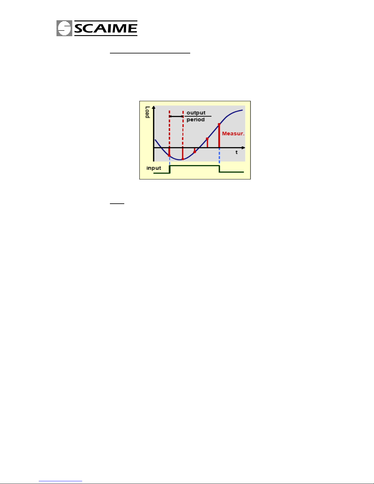
10.2.1 Transmit measurement (Fig. 4)

This is only possible using standard or fast SCMBus format or CANopen protocols. The request can apply to :

- gross measurement

- net measurement

- measurement in A/D converter points

A single measurement is transmitted per rising or falling edge (depending on the configured logic) on the input signal.

Fig. 4

Page 15

eeNNoodd33--D

DDiiggiittaall ddoossiinngg ccoonnttrroolllleer

eNod3-D : User’s instructions 165 752-A 15/23

10.2.2 Measurement window (Fig. 5)

This is only possible using standard or fast SCMBus. The request can apply to :

- gross measurement

- net measurement

- measurement in A/D converter points

While the input is kept at the right level, a series of measurements are transmitted at the period defined by the ‘samplng period’ setting.

10.2.3 Clear

Cancels current tare (same functioning as ‘cancel tare’ command).

Fig. 5

Page 16

eeNNoodd33--D

DDiiggiittaall ddoossiinngg ccoonnttrroolllleer

eNod3-D : User’s instructions 165 752-A 16/23

11 DOSING BY FILLING FUNCTIONING MODE :

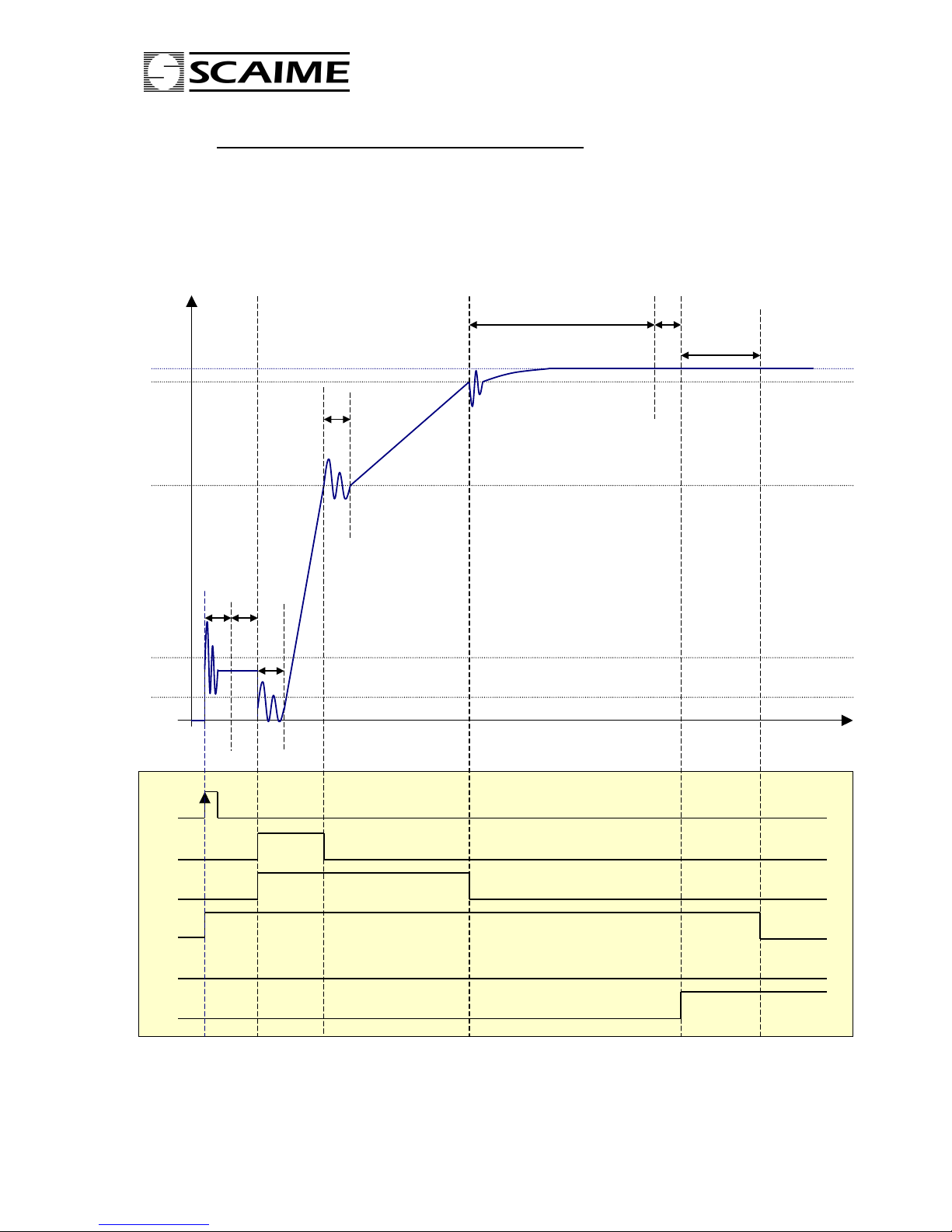
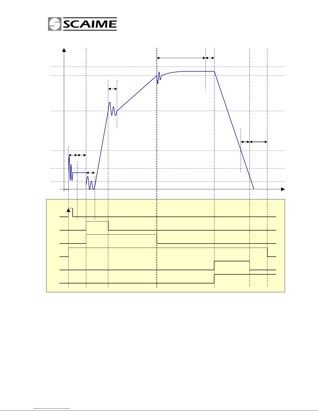
The filling functioning mode is a way to monitor a dosing cycle of a product by measuring the weight of a receptacle placed on a load cell. In this functioning mode, the dosing process is entirely managed by eNod3-D and especially thanks to its four digital outputs allowing to monitor the different phases of the cycle and to indicate errors. Fig. 6 and 7 shown below represent graphically how a filling cycle is working and what is the influence of the variables involved.

Fig. 6 : filling cycle without emptying phase

coarse feed

fine feed

cycle in progress

emptying

dosing result available

start cycle

Time

Measure

2 5

target weight

(target weight – fine feed level)

(target weight – inflight weight)

min empty weight

max empty weight

Page 17

eeNNoodd33--D

DDiiggiittaall ddoossiinngg ccoonnttrroolllleer

eNod3-D : User’s instructions 165 752-A 17/23

∗

1 : start delay

∗ 2 : motion time out ∗ 3 : coarse feed effect neutralization time ∗ 4 : fine feed effect neutralization time ∗ 5 : final stabilization time ∗ 6 : emptying holding time ∗ 7 : end of cycle waiting time

11.1 Starting conditions

After the reception of a ‘start cycle’ command or the activation (rising or falling edge depending on the logic) of a digital input assigned to this function, the filling cycle starts as soon as the ‘start delay’ has elapsed. It also causes an output assigned to the ‘cycle in progress’ function to be set.

Time

Fig. 7

: complete filling cycle with

emptying phase

start cycle

coarse feed

fine feed

cycle in progress

emptying

dosing result available

Measure

2 5

taget weight

(target weight – fine feed level)

(target weight – inflight weight)

emptying end level

min empty weight

max empty weight

Page 18

eeNNoodd33--D

DDiiggiittaall ddoossiinngg ccoonnttrroolllleer

eNod3-D : User’s instructions 165 752-A 18/23

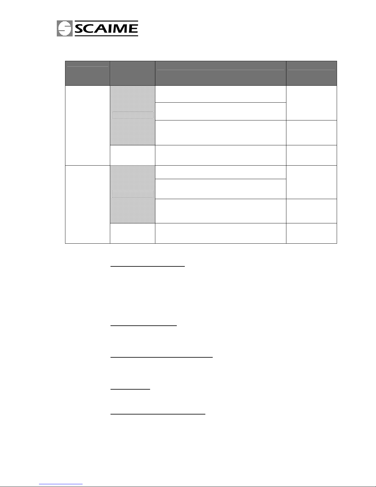
The following tab recaps the possible cases encoutered when starting a cycle :

automatic

taring at start

restart if

suspended

authorization

weight value action

min empty weight < gross weight < max empty

weight

regardless the gross weight value IF

min empty weight = max empty weight = 0

taring then start

other case

cycle cancelled,

error reporting

active

allowed

regardless the gross weight value IF last cycle

was suspended

cycle recovery

from last step

(taring possible)

min empty weight < gross weight < max empty

weight

regardless the gross weight value IF

min empty weight = max empty weight = 0

no tare, starting

from the net

current value

other case

cycle cancelled,

error reporting

inactive

allowed

regardless the gross weight value IF last cycle

was suspended

cycle recovery

from last step

(no tare)

11.2 Cycle description

11.2.1 Flow rate control (optional)

eNod3-D includes a flow rate control system. It makes possible to check that the flow rate during the

cycle is sufficient. The device controls that te flow rate remains equal or superior to a minimal value. If it is not the case, an output assigned to ‘dosing failure’ or ‘flow rate failure’ is set and the cycle is suspended if the cycle recovery option is active else it is stopped. The flow rate control is defined by two parameters :

∗ a time interval (if = 0, the flow rate control is not used) ∗ a minimal weight variation

11.2.2 Automatic taring at start

If the ‘automatic taring at start’ option is active, as soon as the ‘start delay’ has elpased, the tare acquisition is done if measurements are stable. If at the end of the ‘motion time out’ timer, no stability can be found, the tare value is equal to the last net current value.

11.2.3 Coarse feed effect neutralization time

This delay defined in millseconds allows to ignore the effect of the coarse feed starting on the measurement signal and especially the product impact into the receptacle. During this timer, the flow rate control and the level comparisons are inhibited.

11.2.4 Fine feed level

If the level (target weight – fine feed) is crossed the ‘coarse feed’ output is immediately disabled. It is ignored if only the coarse feed is used (cf. §7.4).

11.2.5 Fine feed effect neutralization time

This delay defined in millseconds allows to ignore the effect of the coarse feed ending on the measurement signal and especially the changing in the flow rate. During this timer, the flow rate control and the level comparisons are inhibited.

Page 19

eeNNoodd33--D

DDiiggiittaall ddoossiinngg ccoonnttrroolllleer

eNod3-D : User’s instructions 165 752-A 19/23

11.2.6 Target weight and inflight weight

The ‘fine feed’ disabling occurs when the level (target weight – inflight level) is crossed. The inflight weight value allows therefore to quantify the weight of product that carries on falling after the output inhibition and so to avoid a systematic overoload of the receptacle. This value can be automatically adjusted, the correction amplitude is affected by a percentage that can be configured. It is also possible to have a stronger correction (x 3) as the result is outside the fixed tolerances (cf. §11.2.8).

11.2.7 Final stabilization time

This timer corresponds to the minimal necessary duration for the stabilization of the weight before the determination of the result and the control of tolerances. When it is over, the ‘motion time out’ timer begins. If the stability can not be found within this duration, the dosing result compared to the tolerances is equal to the last net measurement value.

11.2.8 Tolerances

The dosing result is compared to 2 limit values in order to check that it is included within an acceptable range.

∗ a high tolerance (tolérance +) or tolerance in excess :

 if the difference |(target weight – dosing result) > tolérance + |

where (target weight – dosing result) < 0, the ‘out of tolerances’ and ‘dosing failure’ outputs are activated.

∗ a low tolerance (tolérance -) or tolerance in default :

 if the difference |(target weight – dosing result) > tolérance - |

where (target weight – dosing result) > 0, the ‘out of tolerances’ and ‘dosing failure’ outputs are activated. If the ‘use FF if out of low tolerance -’ is active, the fine feed is

restarted. If the updated result is out of tolerances and if the ‘automatic inflight correction’ option is active the inflight weight value is corrected according to the equation :

Once the dosing result is updated and compared to the tolerances an output assigned to the ‘dosing result available’ is set. Then, the cycle ends after the ‘end of cycle waiting time’ or the emptying phase begins.

11.2.9 End of emptying level and emptying holding time

During the emptying phase, an output assigned to the ‘emptying’ function remains active until the ‘emptying holding time’ has elpased after that gross measurement has become inferior to the ‘end of emptying level’.

11.2.10 End of cycle waiting time

This timer is triggered after ther control of tolerances if the emptying phase is not used else it takes place just after the ‘emptying holding time’.

11.2.11 Effective end of cycle

11.3 Digital inputs utilization

11.3.1 Start cycle

If all the starting conditions are respected (cf. §11.1), a rising or a falling edge (depending on the configured logic) on this input causes a new feeding cycle to be started else an error is reported by a ‘dosing failure’ output and into a read-only diagnostic register.

11.3.2 Suspend current cycle

This input function has got two different effects :

∗ if the ‘relaunch cycle if suspended’ option is inactive : this edge-active input causes the

feeding cycle to be stopped inhibiting the different outputs involved.

inflight weight = inflight weight + (dosing result

–

target correction) x correction coeff

Page 20

eeNNoodd33--D

DDiiggiittaall ddoossiinngg ccoonnttrroolllleer

eNod3-D : User’s instructions 165 752-A 20/23

∗ else the cycle is suspended until a new request of starting the cycle that causes the cycle to

continue from its last step.

11.3.3 Stop cycle

This edge-active input causes the feeding cycle to be stopped inhibiting the different outputs involved.

12 DOSING BY UNLOADING FUNCTIONING MODE :

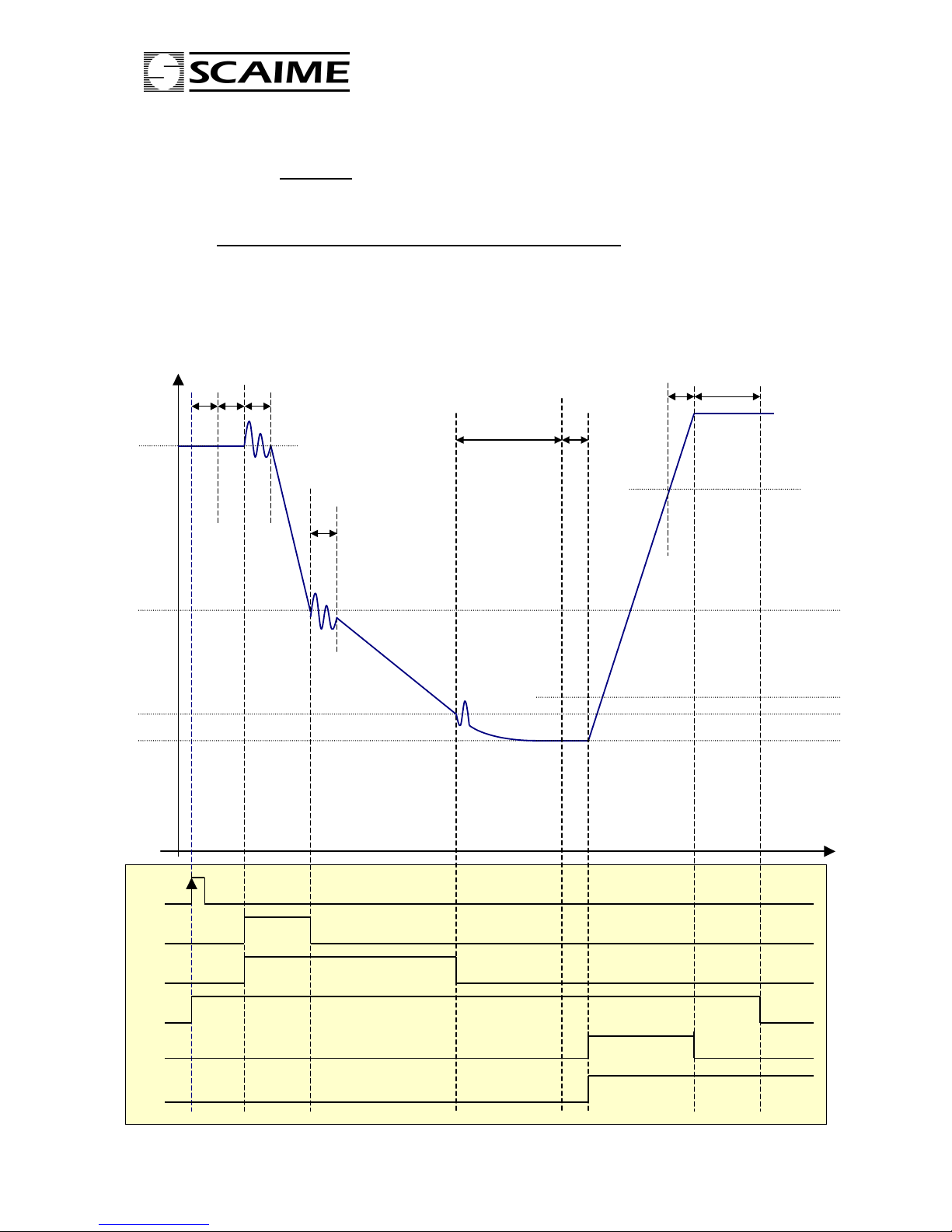
The dosing by unloading functioning mode is a way to monitor a dosing cycle of a product by measuring the weight in loss from a tank equiped with a load cell. In this functioning mode, the dosing process is entirely managed by eNod3-D and especially thanks to its four digital outputs allowing to monitor the different phases of the cycle and to indicate errors. Fig. 8 and 9 shown below represent graphically how a dosing by unloading cycle is working and what is the influence of the variables involved.

Measure

reloading max. level

Time

Fig. 8 : dosing by unloading cycle with reloading phase at the end of the cycle

coarse feed

fine feed

cycle in progress

reloading

dosing result available

start cycle

target weight

(target weight – fine feed level))

(target weight – inflight weight)

reloading min. level

reference weight

dosing result

Page 21

eeNNoodd33--D

DDiiggiittaall ddoossiinngg ccoonnttrroolllleer

eNod3-D : User’s instructions 165 752-A 21/23

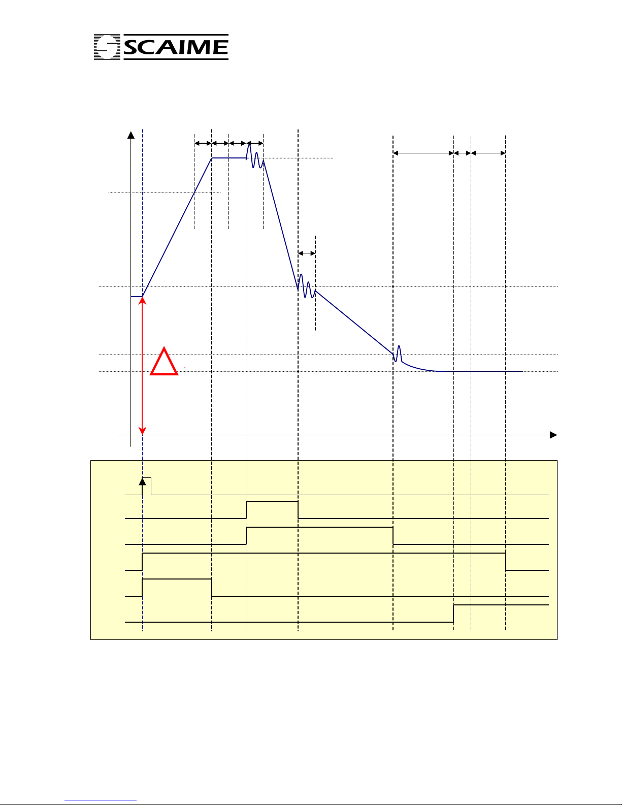
Note : Except the ‘reloading max and min levels’, the variables set used for delimiting the phases of the cycle on the graph are related to the reference weight.

∗ 1 : reloading holding time ∗ 2 : start delay ∗ 3 : motion time out ∗

4 : coarse feed effect neutralization time

∗ 5 : fine feed effect neutralization time

cycle in progress

reloading

dosing result available

start cycle

Fig. 9

: dosing by unloading cycle with reloading phase at the start of the cycle

reloading max. level

coarse flow

fine flow

Time

Measure

3 1

target weight

(target weight – fine feed level)

(target weight – inflight weight)

reference weight

dosing result

target weight + residual weight > gross

Page 22

eeNNoodd33--D

DDiiggiittaall ddoossiinngg ccoonnttrroolllleer

eNod3-D : User’s instructions 165 752-A 22/23

∗

6 : final stabilization time

∗ 7 : end of cycle waiting time

12.1 Reloading management

eNod3-D provides two mechanisms (optional) for reloading management.They allow eNod3-D to enter a

reloading phase in case of a lack of product in the tank.

12.1.1 Reloading at the end of the cycle

An output assigned to the ‘reloading’ function is automatically set if after the result determination the gross measurement is inferior to the ‘reloading min level’. The output remains active until the end of the ‘reloading holding time’ that begins immediately after that the ‘reloading max level’ has been exceeded.

12.1.2 Reloading at the start of the cycle

At every cycle start, eNod3-D checks that there is enough product to reach the dosing target weight. Else if the reloading mode is set to ‘at the start of the cycle’, an output assigned to the ‘reloading’ function is automatically set active until the gross measurement gets superior to the ‘reloading max level’. It remains then active during the ‘reloading holding time’. After the reloading phase end, the dosing cycle begins normally.

12.2 Cycle description

12.2.1 Flow rate control (optional)

eNod3-D includes a flow rate control system. It makes possible to check that the flow rate during the

∗ a time interval (if = 0, the flow rate control is not used) ∗ a minimal weight variation

12.2.2 Verification of the available product quantity

At every cycle start, eNod3-D checks that there is enough product to reach the dosing target weight. If the gross measurement is inferior to the amount (target weight + residual weight), three different cases can occur depending on the selected reloading mode :

 none : an error is reported by an output assigned to the ‘dosing failure’ function and into a

read-only diagnostic register. The new cycle is aborted.

 at the end of the cycle : an error is reported by an output assigned to the ‘dosing failure’

function and into a read-only diagnostic register. The new cycle is aborted.

 at the start of the cycle : eNod3-D starts the reloading phase (cf. §12.1.2).

12.2.3 Start delay

When the ‘start delay’ is over the reference weight acquisition is done if measurements are stable. If at the end of the ‘motion time out’ timer, no stability can be found, the reference weight value is equal to the gross measurement current value

12.2.4 Coarse feed effect neutralization time

This delay defined in millseconds allows to ignore the effect on the measurement signal of the coarse feed starting. During this timer, the flow rate control and the level comparisons are inhibited.

12.2.5 Fine feed level

If the gross measurement decreasing gets superior to (target weight – fine feed level), the ‘coarse feed’ output is immediately disabled.

(↔ reference weight – gross measurement ≥ (target weight – fine feed level ))

It is ignored if only the coarse feed is used (cf. §7.4).

12.2.6 Fine feed effect neutralization time

Page 23

eeNNoodd33--D

DDiiggiittaall ddoossiinngg ccoonnttrroolllleer

eNod3-D : User’s instructions 165 752-A 23/23

12.2.7 Target weight and inflight weight

The ‘fine feed’ ddisabling occurs when the gross measurement decreasing is superior to the (target weight – inflight level) level. The inflight weight value allows therefore to quantify the weight of product

that carries on falling after the output inhibition and so to avoid a systematic overoload. This value can be automatically adjusted, the correction amplitude is affected by a percentage that can be configured. It is also possible to have a stronger correction (x 3) as the result is outside the fixed tolerances (cf. §12.29).

(↔ reference weight – gross measurement ≥ (target weight – inflight level))

12.2.8 Final stabilization time

12.2.9 Tolerances

The dosing result is compared to 2 limit values in order to check that it is included within an acceptable range.

∗ a high tolerance (tolérance +) or tolerance in excess :

 if the difference |(target weight – dosing result) > tolérance + |

where (target weight – dosing result) < 0, the ‘out of tolerances’ and ‘dosing failure’

outputs are activated.

∗ a low tolerance (tolérance -) or tolerance in default :

 if the difference |(target weight – dosing result) > tolérance - |

where (target weight – dosing result) > 0, the ‘out of tolerances’ and ‘dosing failure’

outputs are activated. If the ‘use FF if out of low tolerance -’ is active, the fine feed is

restarted.

12.2.10 End of cycle waiting time

This timer is triggered after ther control of tolerances or after the end of the reloading phase if the reloading mode is set to ‘at the end of the cycle’.

12.2.11 Effective end of the cycle

When the ‘end of cycle wating time’ is over, an output assigned to the ‘cycle in progress’ function is disabled and the statistic variables (number of cycles, average value, running total and standard deviation) are updated. If the reloading mode is set to ‘at the end of the cycle’ and if the gross measurement is inferior to the

‘reloading min level’, the reloading phase starts (cf. §12.1.1) and the effective end of the cycle (‘cycle in progress’ inhibition and statistic variables update) occurs when this phase is over.

12.3 Digital inputs utilization

12.3.1 Start cycle

If all the starting conditions are respected (cf. §12.2.2), a rising or a falling edge (depending on the configured logic) on this input causes a new dosing by unloading cycle to be started else an error is reported by a ‘dosing failure’ output and into a read-only diagnostic register.

12.3.2 Suspend current cycle

This input function has got two different effects :

∗ if the ‘relaunch cycle if suspended’ option is inactive : this edge-active input causes the

feeding cycle to be stopped inhibiting the different outputs involved.

∗ else the cycle is suspended until a new request of starting the cycle that causes the cycle to

continu from its last step.

12.3.3 Stop cycle

This edge-active input causes the feeding cycle to be stopped inhibiting the different outputs involved.