Satec System 295,PM295 Installation And Operation Manual

Download

System 295

Powermeter &

Harmonic Analyzer

Installation and

Operation Manual

BG0130 Rev. A2

SYSTEM 295 POWERMETER

& HARMONIC ANALYZER

Installation & Operation Manual

LIMITED WARRANTY

The manufacturer offers the customer an 24-month functional warranty on the instrument for faulty workmanship or parts from date of dispatch from the distributor. In all cases, this warranty is valid for 36 months from the date of production. This warranty is on a return to factory basis.

The manufacturer does not accept liability for any damage caused by instrument malfunction. The manufacturer accepts no responsibility for the suitability of the instrument to the application for which it was purchased.

Failure to install, setup or operate the instrument according to the instructions herein will void the warranty.

Your instrument may be opened only by a duly authorized representative of the manufacturer. The unit should only be opened in a fully anti-static environment. Failure to do so may damage the electronic components and will void the warranty.

NOTE

The greatest care has been taken to manufacture and calibrate your instrument. However, these instructions do not cover all possible contingencies that may arise during installation, operation or maintenance, and all details and variations of this equipment are not covered by these instructions.

For additional information regarding installation, operation or maintenance of this instrument, contact the manufacturer or your local representative or distributor.

IMPORTANT Please read instructions contained in this manual before performing

installation, and take note of the following precautions:

1. Ensure that all incoming AC power and other power sources are turned OFF

before performing any work on the instrument. Failure to do so may result in serious or even fatal injury and/or equipment damage.

2. Before connecting the instrument to the power source, check the labels on the

side of the instrument to ensure that your instrument is equipped with the appropriate power supply voltage, input voltages, currents, analog output and communication protocol for your application.

3. Under no circumstances should the instrument be connected to a power

source if it is damaged.

4. To prevent potential fire or shock hazard, do not expose the instrument to

rain or moisture.

Introduction 3

5. The secondary of an external current transformer must never be allowed to be

open circuit when the primary is energized. An open circuit can cause high voltages, possibly resulting in equipment damage, fire and even serious or fatal injury. Ensure that the current transformer wiring is made through shorting switches and is secured using an external strain relief to reduce mechanical strain on the screw terminals, if necessary.

6. Setup procedures must be performed only by qualified personnel familiar

with the instrument and its associated electrical equipment.

7. DO NOT attempt to open the instrument under any circumstances. Modbus is a trademark of Modicon, Inc.

F Read through this manual thoroughly before connecting the meter to

the current carrying circuits. During operation of the meter, hazardous voltages are present on input terminals. Failure to observe precautions can result in serious or even fatal injury or damage to equipment.

BG0130 Rev. A2

About This Manual

Chapter 1, Introduction, includes a description of the PM295 basic features. Chapter 2, Installation, provides instructions for mounting, installing and

interfacing the PM295. Chapter 3, Operating the PM295, contains an overview of the PM295 measurement

and operation techniques. Chapter 4, Operation Techniques, provides instructions on the manual operation of

the PM295. Chapter 5 describes Communications Operation. Chapter 6 provides Technical Specifications of the PM295.

Appendices

Appendix A specifies all of the display formats available for operational mode and shows the corresponding front panel displays.

Appendix B lists the instrument programmable parameters that can be accessed either through the front panel or communications.

Appendix C provides a sample of setpoint programming form. Appendices D, E and F contain cable drawings for computer, printer and modem

communications connections.

Related Manuals

This operating manual contains information required for installation and operation of the PM295. Information concerning the serial communications protocols is found in the documents: "System 295 Powermeter and Harmonic Analyzer - ASCII

Communications Protocol - User's Guide" and "System 295 Powermeter and Harmonic Analyzer - Modbus Communications Protocol - User's Guide" shipped with your PM295 on diskette in Microsoft Word document format.

Introduction 1

Table of Contents

1. Introduction...............................................................................................1

1.1 About The PM295..................................................................................1

1.2 Instrument Features Summary...............................................................1

1.3 Measurement Capabilities......................................................................5

2. Installation...............................................................................................11

2.1 Initial Inspection................................................................................... 11

2.2 Mechanical Installation......................................................................... 11

2.3 Input/Output Terminals.........................................................................14

2.4 Power Source Connection....................................................................15

2.5 Voltage Input Connections ...................................................................15

2.5.1 660V Input..............................................................................................15

2.5.2 120V Input..............................................................................................16

2.6 Current Input Connections....................................................................16

2.7 Harmonic Measurement Connections...................................................17

2.8 Wiring Configurations...........................................................................18

2.9 Auxiliary Current Input Connections.....................................................25

2.10 Analog Output Connections.................................................................. 26

2.11 Relay Output Connections....................................................................27

2.12 Discrete Input Connections...................................................................28

2.13 Communications.................................................................................. 28

3. Operating The PM295.............................................................................30

3.1 Instrument Turn On..............................................................................30

3.2 Operational Mode.................................................................................30

3.2.1 Front Panel Operation.............................................................................30

3.2.2 Selecting a Display Page.........................................................................31

3.2.3 Display Formats......................................................................................31

3.3 Programming Mode..............................................................................32

3.3.1 Front Panel Operation.............................................................................32

3.3.2 General Operations.................................................................................34

3.3.3 Menu Map..............................................................................................35

3.3.4 Entering/Quitting Programming Mode......................................................35

3.3.5 Entering the Password............................................................................37

3.3.6 Selecting the Setup Group......................................................................37

3.3.7 Basic Setup ............................................................................................38

3.3.8 Serial Port Setup.....................................................................................39

3.3.9 Discrete Input Setup ...............................................................................39

3.3.10 Counter Setup ........................................................................................41

3.3.11 Analog Output Setup...............................................................................41

3.3.12 Analog Expander Setup ..........................................................................43

3.3.13 Pulsing Relay Setup................................................................................44

3.3.14 Event/Alarm Setpoints.............................................................................45

3.3.15 Timer Setup............................................................................................51

3.3.16 Real Time Clock Setup............................................................................51

3.3.17 Date Format Setup .................................................................................53

3.3.18 Reset Functions......................................................................................53

3.3.19 Password Protection Control...................................................................54

3.4 Self-Test Diagnostics...........................................................................55

4. Operation Techniques............................................................................ 56

4.1 Sampling Technique............................................................................ 56

4.2 Measurement Modes............................................................................56

4.2.1 Real-time RMS Measurements................................................................56

4.2.2 Averaging...............................................................................................57

4.2.3 Minimum/Maximum Logging....................................................................57

4.3 Demand Measurements.......................................................................58

4.3.1 Demand Readings ..................................................................................58

4.3.2 Block Interval Demand............................................................................58

4.3.3 Sliding Window Demand..........................................................................59

4.3.4 Thermal Demand....................................................................................59

4.3.5 Accumulated and Predicted Demands.....................................................60

4.3.6 Demand Interval Measurement ...............................................................61

4.3.7 Resetting the Demands...........................................................................62

4.3.8 Demand Interval Pulse............................................................................63

4.4 Energy Measurements......................................................................... 63

4.4.1 Measurement Modes..............................................................................63

4.4.2 Resetting the Energies............................................................................64

4.4.3 Energy Pulsing........................................................................................64

4.5 Harmonic Measurements..................................................................... 64

4.5.1 Measurement Technique.........................................................................64

4.5.2 Harmonic Parameters.............................................................................65

4.5.3 Real-time Waveform Capture..................................................................66

4.6 Auxiliary Measurements.......................................................................66

4.6.1 Voltage and Current Unbalance...............................................................66

4.6.2 Calculated Neutral Current......................................................................67

4.6.3 Auxiliary Current Input Operation.............................................................67

4.6.4 Frequency Measurements.......................................................................67

4.6.5 Phase Rotation.......................................................................................68

4.6.6 Phase Angles..........................................................................................68

4.7 Time-Of-Use System ...........................................................................68

4.7.1 TOU System Operation...........................................................................68

4.7.2 TOU System Registers ...........................................................................69

4.7.3 TOU Calendars.......................................................................................70

4.7.4 Daily Profiles...........................................................................................70

4.7.5 Connecting with Energy-counting Meters.................................................70

4.7.6 Tariff Interval Pulse.................................................................................70

4.8 Discrete Input Operation ......................................................................70

4.9 Relay Output Operation........................................................................71

4.10 Analog Output Operation......................................................................72

4.11 Analog Expander Operation................................................................. 74

4.12 Counter Operation................................................................................75

4.13 Timer Operation...................................................................................75

Introduction 3

4.14 User Programmable Events .................................................................76

4.15 On-Board Data Recording....................................................................77

4.15.1 Event Logging.........................................................................................79

4.15.2 Data Logging..........................................................................................80

4.15.3 High-speed Waveform Logging...............................................................81

4.15.4 High-resolution Waveform Logging..........................................................82

4.16 Monitoring And Recording Disturbances...............................................82

4.16.1 Disturbance Analysis...............................................................................82

4.16.2 Monitoring Disturbances..........................................................................83

4.16.3 Recording Disturbances..........................................................................83

4.17 Setpoint Operation...............................................................................84

4.17.1 General ..................................................................................................84

4.17.2 Setpoint Programming.............................................................................84

4.17.3 Triggering Conditions ..............................................................................85

4.17.4 Delaying Setpoint Operations..................................................................88

4.17.5 Setpoint Actions......................................................................................88

4.17.6 Special Considerations............................................................................90

4.17.7 Setpoint Programming Techniques..........................................................91

4.18 Update Rates And Response Time.......................................................99

5. Communications Operation................................................................. 101

5.1 General.............................................................................................. 101

5.2 Eia Interface Standards...................................................................... 101

5.2.1 EIA RS-232 Standard............................................................................101

5.2.2 EIA RS-422 and EIA RS-485 Standards................................................102

5.3 Configuring The Communications Port............................................... 102

5.3.1 Communications Mode..........................................................................102

5.3.2 Interface...............................................................................................103

5.3.3 Communication Address .......................................................................103

5.3.4 Baud Rate ............................................................................................103

5.3.5 Data Format .........................................................................................104

5.3.6 Handshaking.........................................................................................104

5.3.7 DTR/RTS Control Line ..........................................................................105

5.3.8 Configuring the Printer Parameters........................................................105

5.4 Response Time..................................................................................106

5.5 Print Mode......................................................................................... 106

6. Technical Specifications...................................................................... 108

Appendix A Display Formats....................................................................... 113

Appendix B Programmable Parameters...................................................... 124

Appendix C Setpoint Programming Form...................................................... 152

Appendix D Cable Drawings - Computer Connection...................................153

Appendix E Cable Drawings - Serial Printer Connection.............................. 159

Appendix F Cable Drawings - Modem Connection.......................................163

INDEX..........................................................................................................164

Introduction 1

1. Introduction

1.1 About The PM295

The PM295 is an advanced microprocessor-based digital instrument that incorporates the capabilities of the network analyzer, data recorder and programmable controller allowing for user network monitoring, analysis and control. The instrument provides three-phase measurements of electrical quantities in power distribution systems, monitoring external events, operating external equipment via relay contacts, fast and long-term on-board recording of measured quantities and events, harmonic network analysis and disturbance recording.

The PM295 can communicate with PLCs and PC based workstations via serial communications and directly by transducing analog and discrete signals, serving as excellent partner in power network management. All measurement functions of the PM295 are remotely programmable via the communications port.

The accompanying PAS295 software package provides easy remote programming for the instrument, data acquisition, analysis and on-screen presentation.

1.2 Instrument Features Summary

Processing Block

• CPU - microcontroller 80C196KC20 with a 20 MHz oscillator

• Extended nonvolatile RAM with battery backup for data recording - 512K byte

module

• On-board real-time clock

• A I0-bit A/D converter

• Power supervisory circuit

• External watch-dog

Analog Inputs

• 3 isolated voltage inputs - 660 VAC/120 VAC options

• 3 isolated current inputs - 1A or 5A secondary options

• 1 isolated auxiliary current input for ground leakage/neutral current

measurements - 5 mA/1A/5A secondary options (upon order)

Discrete Inputs

• 8 programmable optically isolated digital inputs free programmable for sensing external contacts’ status and pulses.

Applications:

- monitoring external dry contacts

- sensing an external synchronization pulse for demand interval measurements

- counting external pulses

- connecting with external energy-counting meters

- triggering setpoints from external alarm/event sources

- selecting output values for internal multiplexed analog output

Analog Outputs

• one internal multiplexed scalable free-programmable optically isolated current output - 0-20/4-20 mA (upon order). Provides time-sharing output for up to 16 analog parameters that can be controlled externally by a combination of binary signals on the instrument's discrete inputs (from 1 to 4 inputs can be operated)

• extension for up to 14 analog outputs is available using external analog expanders (up to 2 units per instrument)

Discrete Outputs

• 4 digital free-programmable relay outputs (dry contact)

Applications:

- alarm activations

- load control

- energy pulsing

- time reference pulses for synchronization demand and tariff calculations

Timers

• 4 programmable a 1 sec resolution timers for repeated setpoint operations and data recording

Counters

• 8 programmable large-scale counters with scalable input for counting input pulses and various internal events

User Programmable Events

• 8 programmable flags for asserting user-definable events, allowing manual control and expansion of setpoint operations

Introduction 3

Setpoints

• 16 programmable setpoints for monitoring various events:

- up to 4 triggering conditions for each setpoint combined by OR/AND logical operations

- up to 4 actions for each setpoint on setpoint operation

- programmable hysteresis (dead-band) for analog triggers

- programmable delay for setpoint operation/release

• each setpoint can be combined with other setpoints if extended number of conditions or actions needed

• any measured or sensed quantity/status/pulse/event can be used as a trigger condition for setpoint operation

• voltage disturbance and phase rotation monitoring are available for triggering setpoint operations

• setpoint actions available:

- operating relay output

- increment/decrement/clear counter

- assert/clear user programmable event

- reset total accumulating energy registers

- reset extreme demand registers

- reset TOU system accumulating energy registers

- reset TOU system demand registers

- clear all counters

- clear Min/Max log registers

- event logging on setpoint operation

- data logging in selected data log partition

- high-speed waveform logging for disturbance analysis

- high-resolution waveform logging for harmonic analysis

• each setpoint can be programmed to be operated manually via communications by overriding present conditions or by gating setpoint operations in addition to other setpoint conditions (for example when event/data recording is needed for a user-defined time interval)

• each setpoint can be programmed to allow the setpoint operations to be recorded in the event log on any setpoint transition - operate, release or either transition

On-board Data Recording

• 19 free-programmable extended memory partitions for recording events, measured data, and captured waveforms:

- one event logging partition for recording various events and setpoint operations, providing storage for up to 36864 events with a 512K memory module (assuming the entire memory allocated for the partition)

- 16 programmable data logging partitions, each for recording from 1 to 16 user programmable parameters per record, providing total storage for up to 114,688 parameters with a 512K memory module (assuming the entire memory allocated for data logging)

- one partition for high-speed waveform recording (32 samples x 16 cycles x 6 inputs per record) for disturbance analysis, and one partition for high-resolution waveform recording (128 samples x 4 cycles x 6 inputs per record) for harmonic analysis, each providing storage for up to 19, 40, or 82 records with a 512K memory module (assuming the entire memory allocated for the partition)

• each memory partition can be sized to store desired number of records, from 1 record and up to the entire memory size, using an arbitrary combination of partitions

• each memory partition can be programmed to store the oldest records without overwriting previously recorded data when a partition is filled up, or to wrap around by writing new records over the oldest records so that stored records will always contain the most recent data

Time-of-Use System

• 8 programmable accumulating energy registers for 16 tariffs, each configurable for counting kWh/kvarh/kVAh or pulses from up to 8 external energy-counting meters

• 3 programmable demand registers for 16 tariffs, configurable for recording extreme (minimum and maximum) demands using varying calculation techniques: block interval/sliding window/thermal demand

• 16 daily profiles (types of days) with up to 8 tariff changes per day

• 2-year calendar

Communications

• one programmable optically isolated serial port - RS-232/RS-422/RS-485 embedded options with a user-selectable baud rate of 110 to 38400 BPS

Display

• multi-page display composed of 11 windows with high-brightness seven- segment digital LEDs. A total of 55 display pages are available

Keypad

• four membrane long-life push-buttons for page scrolling and programming

Power Supply

• 90-264 V AC, 10-290 V DC options

Introduction 5

1.3 Measurement Capabilities

Table 1-1 lists quantities and signals measured, calculated and sensed by the PM295. Measurement readings can be accessed via the front panel and communications. These readings can also be transferred through internal analog and relay outputs, and used as triggers for alarm/event setpoint operations. Ranges and full scale values for measurement parameters are summarized in technical specifications (see Chapter 6). Chapter 3 describes measurement functions and modes of measuring input values.

Table 1-1 Measured Quantities and Sensed Signals

Measurement Mode Usage/output

Parameter Real-

time

Sliding

average

Demand Min/

Max

Display Commu-

nications

Analog

output

Pulse Data

logging

Trigger

setpoint

Per phase Measurements Voltage (L-N/L-L) À

• • • • • • • • •

Current

• • • • • • • • •

kW Á

• • • • • • • •

kvar Á

• • • • • • • •

kVA Á

• • • • • • • •

Power factor (signed) Á

• • • • • • • •

Voltage THD Â

• • • • • • • •

Current THD

• • • • • • • •

K-Factor

• • • • • • • •

Three-phase total measurements Total kW

• • • • • • • • •

Total kvar

• • • • • • • • •

Total kVA

• • • • • • • • •

Total power factor signed

• • • • • • • •

Total power factor lag

• • • • • • •

Table 1-1 Measured Quantities and Sensed Signals

Measurement Mode Usage/output

Parameter Real-

time

Sliding

average

Demand Min/

Max

Display Commu-

nications

Analog

output

Pulse Data

logging

Trigger

setpoint

Total power factor lead

• • • • • • •

Auxiliary measurements Auxiliary current (ground

leakage/neutral current)

• • • • • • • •

Neutral current (calculated)

• • • • • • • •

Frequency

• • • • • • • •

Voltage unbalance

• • • • • • • •

Current unbalance

• • • • • • • •

Low values on any phase

Low voltage (L-N/L-L) À

• • • • •

Low current

• • • • •

Low kW Á

• • • • •

Low kvar Á

• • • • •

Low kVA Á

• • • • •

Low power factor lag Á

• • • • •

Low power factor lead Á

• • • • •

Low voltage THD Â

• • • • •

Low current THD

• • • • •

Low K-Factor

• • • • •

High values on any phase High voltage (L-N/L-L) À

• • • • •

High current

• • • • •

High kW Á

• • • • •

High kvar Á

• • • • •

Introduction 7

Table 1-1 Measured Quantities and Sensed Signals

Measurement Mode Usage/output

Parameter Real-

time

Sliding

average

Demand Min/

Max

Display Commu-

nications

Analog

output

Pulse Data

logging

Trigger

setpoint

High kVA Á

• • • • •

High power factor lag Á

• • • • •

High power factor lead Á

• • • • •

High voltage THD Â

• • • • •

High current THD

• • • • •

High K-Factor

• • • • •

Demands Volt demand per phase À

• • • Ã • • • •

Ampere demand per phase

• • • Ã • • • •

Total kW demand (block interval, sliding window, thermal)

• • • Ã • • • •

Total kvar demand (block interval, sliding window, thermal)

• • • Ã • • • •

Total kVA demand (block interval, sliding window, thermal)

• • • Ã • • • •

Predicted demands Total kW demand (accumulated,

sliding window)

• • • • • •

Total kvar demand (accumulated, sliding window)

• • • • • •

Total kVA demand (accumulated, sliding window)

• • • • • •

Total energies kWh (import, export, net, total)

• • • • •

Table 1-1 Measured Quantities and Sensed Signals

Measurement Mode Usage/output

Parameter Real-

time

Sliding

average

Demand Min/

Max

Display Commu-

nications

Analog

output

Pulse Data

logging

Trigger

setpoint

kvarh (import, export, net, total)

• • • • •

kVAh (total)

• • • • •

Per phase harmonic measurements Voltage harmonics (1-40), % Â

• • Ä • • • •

Current harmonics (1-40), %

• • Ä • • • •

Harmonic voltages (for odd harmonics 1-39) Â

• • Ä • • • • •

Harmonic currents (for odd harmonics 1-39)

• • Ä • • • • •

Three-phase total harmonic measurements Harmonic total kW (for odd

harmonics 1-39)

• • Ä • • • • •

Harmonic total kvar (for odd harmonics 1-39)

• • Ä • • • • •

Harmonic total power factors (for odd harmonics 1-39)

• • Ä • • • • •

TOU energy registers 8 registers for 16 tariffs, free

programmable for counting kWh/kvarh/kVAh or pulses from external energy-counting meters

• •

TOU demand registers 3 registers ( kW/kvar/kVA demands)

for 16 tariffs, free

• • • •

programmable for registration block interval/sliding window/ thermal Min/Max demands

• • •

Introduction 9

Table 1-1 Measured Quantities and Sensed Signals

Measurement Mode Usage/output

Parameter Real-

time

Sliding

average

Demand Min/

Max

Display Commu-

nications

Analog

output

Pulse Data

logging

Trigger

setpoint

TOU system parameters Active tariff

• • •

Active profile

• • •

Pulse counters 8 large scale counters for counting

external pulses or internal events

• • • •

Discrete inputs 8 discrete inputs, free configurable for

sensing external contacts or pulses

• • • •

Timers 4 timers with 1 sec resolution

•

Internal events kWh pulse (import/export/total)

• •

kvarh pulse (import/export/total)

• •

kVAh pulse

• •

Start demand interval

• •

Start tariff interval

• •

Time/date parameters Year, month, day of month, day of

week, hour, minute, second

•

Special measurements Voltage disturbance

•

Phase rotation

• •

Phase angles per phase

•

NOTES

¬ For all applications/outputs, the voltage parameters can represent line-to-neutral or line-to-line voltages depending on the

wiring configuration selected in the Powermeter. (4Ln3/3Ln3 = line-to-neutral voltages; all other configurations = line-to-line voltages).

- In 3-wire connection schemes, the individual phase values for power factor, active power, apparent power and reactive power will be zero, because they have no meaning. Only total three-phase power values can be used.

® In all grounded connections using either 4Ln3 or 4LL3 wiring configurations, harmonic voltages will represent line-to-neutral

voltages. In a 3-wire direct connection, harmonic voltages will represent line-to-neutral voltages that arise on the Powermeter's input transformers. In a 3-wire open delta connection, harmonic voltages will comprise L12 and L23 line-to-line voltages.

¯ Display readings are the maximum demands over entire time of survey. ° Measurements can be made via 16 programmable Min/Max registers.

Installation 11

2. Installation

2.1 Initial Inspection

Upon receipt, the instrument should be free of damage and in perfect order. To confirm this, first inspect the instrument for physical damage incurred in transit. If the instrument is damaged, inform your local distributor immediately. Only after you have determined that the instrument is damage-free, test the electrical performance.

2.2 Mechanical Installation

Location

The instrument should be mounted away from heat sources in a dirt-free environment. The instrument should not be operated in direct sunlight nor should it come into contact with oil or moisture.

Although designed to operate in an electrically noisy environment, the instrument should not be placed near very high electric fields. It must be placed at least one-half meter (1.64 feet) from current lines carrying up to 600 amperes. For currents greater than 600A and up to 2,000A, this distance must be at least 1 meter (3.28 feet).

In the event that the instrument is mounted in a harsh, noisy environment with high potential for electromagnetic impulses from heavy switch gears, motors or lightning, it is recommended to install appropriate protective devices such as lightening and over-voltage arresters to all incoming voltage inputs.

Mounting

The PM295 is designed to be panel mounted. The dimensions of the cutout necessary both for front (standard) and rear panel mounting are shown in Figures 2- 1 and 2-2.

For either front or rear mounting, the instrument is positioned through the cutout, and the bracket(s) are then screwed to the back of the instrument as shown in the figures. For front mounting, the four thrust screws are tightened against the panel to affix the instrument in place.

Figure 2-1 Front Mounting (standard)

Installation 13

Figure 2-2 Rear Mounting

Step 1

Connect the bracket to the instrument

Step 2

Mount the O-ring on the instrument

Step 3

2.3 Input/Output Terminals

Connections to the PM295 are made via terminals located on the back of the instrument as shown in Figure 2-3 and detailed in Figure 2-4.

Figure 2-3 Location of Terminal Strips and Communications Connector

Figure 2-4 Connection Terminal #1

Installation 15

2.4 Power Source Connection

The instrument can be operated from any single phase AC power source supplying 90-264 VAC 50/60 Hz, or from DC power supply 10-290 VDC. Power supply options are available upon order.

For the power source wiring, see Figure 2-4. If an AC power supply is used, the live line of the control power should be connected to terminal 1 and the neutral to terminal 3. If a DC power supply is used, the positive supply wire should be connected to terminal 1 and the negative wire to terminal 3.

F The ground lug must be connected to the ground.

2.5 Voltage Input Connections

2.5.1 660V Input

Direct Connection

For some power systems, the 660V input option allows the user to use direct connection without applying potential transformers (PT). This will depend on the power system configuration and on the system voltage level. In the case of systems with line-to-line voltage up to 660V, direct connection may be used for 4-wire and 3-wire systems. Wiring diagrams for these are provided in Figures 2.5, 2.8, and 2.9.

F To ensure accurate readings, the measured voltage between terminals

2-11, 5-11 and 8-11 should not exceed RMS value 550 VAC and amplitude value 900V.

NOTE

When direct connection without potential transformers is used, set the PT RATIO in the instrument to 1.

Using Potential Transformers

For high voltage applications (above 660V line-to-line voltage) potential transformers (PT) must be used to scale down the input voltage to rated input scale of the instrument. The instrument is intended to be wired via potential transformers with secondary line-to-line voltage up to 120V +20%. The instrument supports 3- wire open delta systems and 4-wire Wye systems. Wiring diagrams for these are provided in Figures 2-6, 2-7, 2-10 and 2-11.

NOTE

When using potential transformers, the input voltage scale is defined in the instrument by the PT RATIO parameter, which is the relation of the PT primary rated voltage to the secondary rated voltage. For example, using a PT with the ratings of 165 kV : 110 V, the PT RATIO would be 165,000/110 = 1500. The PT RATIO must be specified correctly for the instrument to provide accurate voltage readings.

2.5.2 120V Input

The instrument with the 120V input option is intended to be wired via potential transformers with secondary line-to-line voltage up to 120V +20%.

F To ensure accurate readings, the measured voltage between terminals

2-11, 5-11 and 8-11 should not exceed RMS value 144 VAC and amplitude value 226V.

2.6 Current Input Connections

The PM295 is designed to measure phase currents via external current transformers (CTs) with either 1 A or 5 A secondaries. The current input ratings are factory installed. All current inputs are galvanically isolated using internal current transformers.

Using 3-wire connections, only two current transformers are required. It is also possible to use three current transformers (see Figure 2-7). If necessary, the return side of the current transformers (terminals 3, 6 and 9) may be grounded.

F To ensure accurate readings, the input current should not exceed: for

the 1A secondaries - RMS value 1.2A and amplitude value 1.76A, and for the 5A secondaries - RMS value 6A and amplitude value 8.8A. At least one of the L1 or L3 phase voltages must be connected to provide correct measurements of the current.

F The CTs must be connected in the correct order and with the correct

polarity as shown in the wiring diagrams for the instrument to operate properly. If the instrument displays a power factor of zero or close to it, or if power readings show unreasonable values, the polarity of the CT connections might be reversed.

For the line current inputs overload, see technical specifications in Chapter 6.

NOTE

The phase current input scale is defined in the instrument by the CT PRIMARY CURRENT parameter. It is equal to the primary rating of the current transformer.

Installation 17

2.7 Harmonic Measurement Connections

Harmonic measurements can be made only on signals that are present on the instrument inputs. In some of the 3-wire configurations, there may be one of inputs missing, so the user might not get the appropriate readings.

4-wire Configurations

In 4-wire configurations, no special considerations are necessary. All harmonic quantities will be measured correctly. In the '4Ln3', '4LL3', '3Ln3' or '3LL3' wiring modes, harmonic voltages will represent line-to-neutral voltages. In '3Ln3' or '3LL3' wiring modes, harmonic voltage will be measured only for two phases and the total power harmonics will be calculated inaccurately.

3-wire Direct Connection

In a 3-wire Direct Connection, harmonic voltages will represent the three phase lineto-neutral voltages that appear on the instrument input transformers. If the system

load is not symmetrical, the voltage readings will have no meaning. In the case of the symmetrical load, harmonic voltages will not reflect all the multiples of order 3 harmonic.

Using 2 CTs, harmonic currents will be measured only for two phases and the total power harmonics will be calculated inaccurately.

3-wire Open Delta Connection

Readings for harmonic voltages will represent two line-to-line voltages L12 and L23. Current harmonics will be taken using 2 or 3 CTs, according to the wiring configuration.

Total harmonic powers will be measured properly using two input line-to-line voltages and two currents.

2.8 Wiring Configurations

The WIRING MODE must be set in the instrument in accordance with the wiring configuration. The wrong wiring mode may result in incorrect readings.

There are seven possible wiring configurations:

No. Wiring Configuration Wiring Mode

1 3-wire direct connection using 2 CTs (2-element)

3DIR

2 3-wire open delta connection using 2 PTs, 2 CTs (2-element)

3OP2

3 3-wire open delta connection using 2 PTs, 3 CTs (2½-

element)

3OP3

4 4-wire WYE direct connection using 3 CTs (3-element)

4Ln3 or 4LL3

5 4-wire delta direct connection using 3 CTs (3-element)

4Ln3 or 4LL3

6 4-wire WYE connection using 3 PTs, 3 CTs (3 element)

4Ln3 or 4LL3

7 4-wire WYE connection using 2 PTs, 3 CTs (2½-element)

3Ln3 or 3LL3

In 4-wire configurations, '4Ln3' or '3Ln3' wiring modes represent line-to-neutral voltage readings; '4LL3' or '3LL3' wiring modes represent line-to-line voltages.

For 3-wire configurations, voltage readings will always represent line-to-line voltages. These do not affect readings for harmonic voltages (see Section 2.7).

Installation 19

1) Three Wire Direct Connection Using 2 CTs (2-element)

This connection can be applied to systems with line-to-line voltage up to 660V. The three line voltages are taken at terminals 2, 5 and 8 as shown in Figure 2-5.

Figure 2-5 3-wire Direct Connection Using 2 CTs (2-element) WIRING MODE 3DIR

Readings represent line-to-line voltages. The two line currents are monitored via two CTs. The third current is calculated based on the two measured currents.

2) Three Wire Open Delta Connection Using 2 PTs, 2 CTs (2-element)

This configuration, shown in Figure 2-6, can be used with either 660V or 120V input. Readings represent line-to-line voltages. The two line currents are measured via 2 CTs; the third current [LINE 2(B)] is calculated based on the two measured currents. The common taps of the PT secondaries are connected to terminal 11.

Note the connection between terminals 5 and 11.

Figure 2-6 3-Wire Open Delta Connection Using 2 PTs, 2 CTs (2-element)

WIRING MODE 3OP2

Installation 21

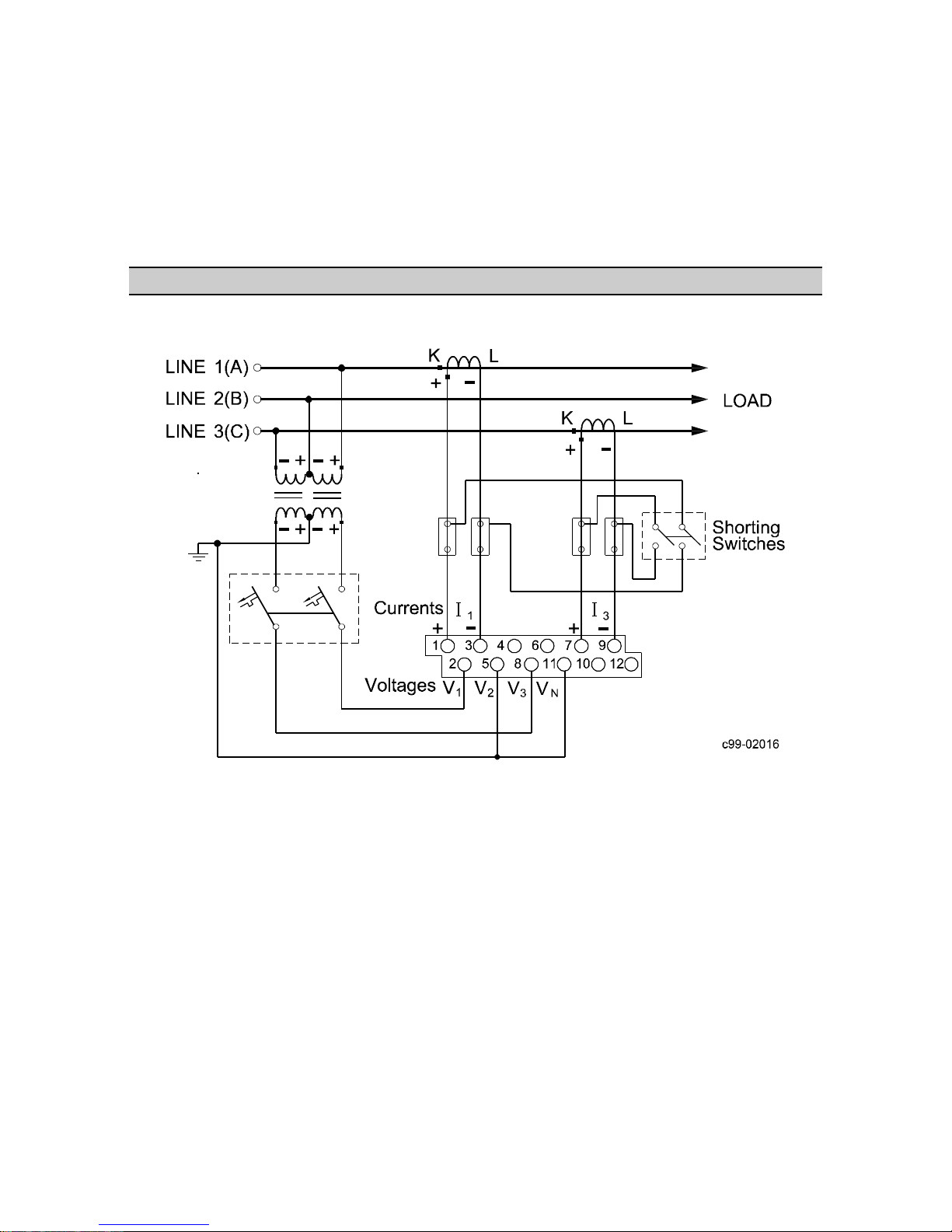
3) Three Wire Open Delta Connection Using 2 PTs, 3 CTs (2½element)

This configuration, shown in Figure 2-7, can be used with either 660V or 120V input. Readings represent line-to-line voltages. All three line currents are measured. The common taps of the PT secondaries are connected to terminal 11.

Note the connection between terminals 5 and 11.

Figure 2-7 3-Wire Open Delta Connection Using 2 PTs, 3 CTs (2½-element)

WIRING MODE 3OP3

4) Four Wire Wye Direct Connection Using 3 CTs (3-element)

The instrument takes the three line-to-neutral voltages and three line currents as shown in Figure 2-8. The system neutral is connected to terminal 11.

Figure 2-8 4-Wire Wye Direct Connection Using 3 CTs (3-element) WIRING MODE 4Ln3/4LL3

Installation 23

5) Four Wire Delta Direct Connection Using 3 CTs (3-element)

The instrument senses the three line-to-neutral voltages and three line currents as shown in Figure 2-9. The system neutral is connected to terminal 11.

Figure 2-9 4-wire Delta Direct Connection Using 3 CTs (3-element)

WIRING MODE 4Ln3/4LL3

6) Four Wire Wye Connection Using 3 PTs, 3 CTs (3-element)

This configuration can be used with either 660V or 120V input. The instrument senses the three line-to-neutral voltages and three line currents as shown in Figure 2-

10. The common taps of the PT secondaries are connected to terminal 11.

Figure 2-10 4-wire Wye Connection Using 3 PTs, 3 CTs (3-element) WIRING MODE 4Ln3/4LL3

Installation 25

7) Four Wire Wye Connection Using 2 PTs, 3 CTs (2½-element)

This configuration can be used with either 660V or 120V input. The instrument senses the 2 line-to-neutral voltages and 3 line currents as shown in Figure 2-11. The common taps of the PT secondaries are connected to terminal 11. This configuration

will provide accurate power measurements only if the voltages are balanced.

Figure 2-11 4-wire Wye Connection Using 2 PTs, 3 CTs (2½-element) WIRING MODE 3Ln3/3LL3

2.9 Auxiliary Current Input Connections

The PM295 can be equipped with an auxiliary current input (optional). Figure 2-12 shows examples of the auxiliary current input connections. This input can be used for direct measurement of either ground leakage or the neutral current.

The secondary rating of the CT connected to the auxiliary current input is either 1 A, 5 A, or 5 mA, as per your order. The CT PRIMARY CURRENT parameter for the auxiliary current input is set in the instrument independently of the phase current inputs.

97-04023

2 5 8

1011

6 7129

+ -

LOAD

L3 (C)

L2 (B)

L1 (A)

123

5 8

4 6

L1 (A) L2 (B) L3 (C)

7 9

+12-

+ -

LOAD

a) Neutral current b) Ground leakage current

Figure 2-12 Auxiliary Current Input Connections

2.10 Analog Output Connections

Figure 2-13 shows wiring for an analog output. The analog output is optically isolated and has an internal source +24 VDC to power the current loop. Analog output range is 0-20 or 4-20 mA, as per your order.

max 510 Ohm

Figure 2-13 Analog Output Connections

The permitted range for the current loop resistance is 0 to 510 Ω. In many industrial applications, it may be necessary to protect the output from

accidental shorts to AC line voltages, in addition to high common-mode voltages. The circuit shown in Figure 2-14 can be used for this purpose.

VR1 = 25 VRMS

VR1

C1 = 0.1 mF/50V

Figure 2-14 Protective Circuit For Analog Output

Installation 27

2.11 Relay Output Connections

The PM295 is equipped with four electromechanical relays. Relays #1, #2, and #4 are two-contact Form A (SPST) relays, and relay #3 is a three-contact Form C (SPDT) relay. Relay #1 is a reed relay that is intended for a small load, for example, to output pulses. For the relay ratings, see technical specifications in Chapter 6. Figure 2-15 illustrates wiring connections for the relays.

All relays are normally de-energized.

K321K1

Figure 2-15 Relay Output Connections

Relay Contact Protection

When using relay outputs for switching lamp, capacitive or inductive circuits, some form of transient suppression may be necessary to keep the relay contacts within the voltage or current ratings. The following diagrams recommend some variants of protective circuits for relay outputs.

LOADVs

Figure 2-16 Inductive load - Zener Diode Protection

LOADsV

Figure 2-17 Inductive load - Diode Protection

LOADsV

Figure 2-18 Inductive Load - Diode/resistor Protection

2.12 Discrete Input Connections

The PM295 provides eight optically isolated dry-contact sensing (voltage-free) discrete inputs. Figure 2-19 shows wiring for discrete inputs.

K1 K2 K3 K4 K5 K6 K7 K8 COM

6 8 1210 14 16 18 20 11

+5 V

0 V

1 kOhm

PM295

Figure 2-19 Discrete Input Connections

The dry contacts connected to discrete inputs must be floating relative to the ground with a minimum rating of 5 VDC, 5 mA. It is also recommended to perform connections using a shielded, twisted pair cable that is isolated from noise sources.

2.13 Communications

Connector Pinout

The communications port is optically isolated and supports both EIA RS-232 and RS-422/485 standard interfaces (user-selectable). The serial interface connector is standard D-type 9 pin female plug-in, located at the top center of the back of the instrument. Tables 2-1 and 2-2 list the pinout of the connector.

NOTE

The functions of pins 4 and 5 can be programmed via keypad upon the needs of the user. Refer to Section 5.3 on how to select the appropriate pin function.

Table 2-1 RS-232 pinout

Pin Name Function

1 0V Common 2 TXD Transmit Data 3 RXD Receive Data 4 DTR/RTS Data Terminal Ready/Request to Send 5 DSR/CTS Data Set Ready/Clear to Send

Installation 29

Table 2-2 RS-422/RS-485 pinout

Pin Name Function

1 0V Common 6 TXD+ + Transmit Data 7 RXD+ + Receive Data 8 TXD - - Transmit Data 9 RXD - - Receive Data

For RS-485 communications, connect together pins 6-7 (TXD+ and RXD+), and pins 8-9 (TXD- and RXD-).

Receive/Transmit Indicators

The PM295 has two LED indicators, showing activity on the serial port lines. They are located to the left of the communications connector. The left LED is connected to the receive line and flashes when the instrument is receiving data, and the right LED is connected to the transmit line and flashes when the instrument is transmitting data.

Cable Connections

For the cable drawings, refer to Appendices D, E and F. For RS-422/RS-485 balanced data transmission, a shielded, twisted pair cable

should be used for each communication link. To minimize reflections and reduce cross talk, it is recommended to terminate the ends of lines with the termination resistor of 200-500 Ω.

For RS-232 connections, a flat cable can be used. The conductor size of the 2 wires shall be 24 AWG or larger with wire resistance

not exceeding 30 Ω per 1000 feet per conductor. When lines are routed through an electrically noisy environment, input protection

against switching or lightening induced surge voltages may be required in addition to line termination.

3. Operating The PM295

3.1 Instrument Turn On

Connect the PM295 to a suitable power source. When power is applied, the PM295 initiates a series of self tests. Upon completion of self tests, all the front panel LEDs light up for one second and indicate a one-digit diagnostic code. An ‘8’ represents normal power up. If a different diagnostic code continually appears when you apply power to the instrument, contact your local distributor. For error codes, refer to Section 3.4.

Upon power up, the PM295 assumes the operational mode.

3.2 Operational Mode

3.2.1 Front Panel Operation

Operational mode is the default mode of the instrument, in which measurement readings appear in the 11 windows on the front panel display. Various display formats can be selected using the front panel keypad. Figure 3-1 shows the front view of the instrument.

Figure 3-1 PM295 Front View

Operating The PM295 31

The instrument keypad consists of four membrane long-life push-buttons allowing the user to perform all of the front panel functions. The following descriptions detail the keys and their functions in operational mode.

UP ARROW t Scrolls display pages forward DOWN ARROW u Scrolls display pages backward SELECT Enters programming mode ENTER Toggles the display between main and subpage level

When a key is pressed, it is entered into a key register, which may be polled through communications.

3.2.2 Selecting a Display Page

The instrument provides a total of 55 display pages, which can be accessed on the two display levels: six pages on the main level, and the remaining pages - on the sub-page level. The active page number is indicated on the display. It illuminates continuously when you are on the main level, and flashes when you enter the subpage level. At power up, the instrument always returns to the page that was last displayed.

To scroll through pages on either level:

Ä Press the up arrow key to scroll forward. Ä Press the down arrow key to scroll backward.

To enter the subpage level:

Ä Press ENTER.

To return to the main level:

Ä Press ENTER once more.

3.2.3 Display Formats

Appendix A specifies all of the pages available for operational mode. Each page is listed with a corresponding front panel display.

The display illustrations indicate the measurement data that can be viewed on a corresponding display page, and the abbreviated window labels and page numbers that appear on display exactly as indicated in illustrations. The measurement data is indicated using a plain style, and the window labels and page numbers are accented

by a boldface. Sub-pages are referred to by the corresponding page number followed by the sub-page number.

Table A-1 in Appendix A contains a cross reference to display pages and lists all parameters that can be accessed via the front panel display with their respective location and available resolution.

3.3 Programming Mode

3.3.1 Front Panel Operation

Programming mode allows the user to configure the instrument for a particular application, and to perform protected management functions such as the resetting of the data keeping registers and the setting of RTC.

Password Protection

Programming mode has various levels of authorization to provide safeguards against unauthorized changes in the instrument setup configuration:

• view level non-protected level: can view all setups and list configuration

parameters. No changes allowed. No password needed.

• protected level can view/modify setups and perform management functions

(reset, RTC update)

• superuser level- privileged level: all functions allowed at the protected level

plus user protection override. This level is intended for service procedures, and is not normally accessed by the user. It is protected by the factory set superuser password.

Entering the protected level is protected by the user password. The user can set password, and disable or enable password control. With password control disabled, the user enters the protected level without password checking.

NOTE

The instrument is shipped with password protection disabled. To restore password protection, the user should explicitly enable password control from the PASSWORD PROTECTION CONTROL menu (see below).

F When password protection is enabled, the instrument automatically

prompts for the password when you attempt to access the protected level. Store your password in a safe place. If you do not provide the correct password, you will need to contact your local distributor for the superuser password to override password protection.

Operating The PM295 33

Menus

Manual operation of the instrument in programming mode is performed through menus.

The following sections in this chapter specify all of the menus available for the instrument programming via the front panel. Each PM295 menu is listed with a corresponding front panel display. Menus that require values to be input show the applicable range limits. A map illustrating the instrument menus is provided in Section 3.3.3.

Display in Programming Mode

Menus normally appear in windows 4 through 6, where menu items are indicated. Each window can represent one of three types of display controls:

• static window - a labeled window identifying the displayed menu. Static

window may not be accessed with the front panel keys.

• button-window - a labeled window allowing the user to perform an action, to

enter or quit a menu. Button-window acts as labeled button and displays an abbreviated character label of the action or menu entry.

• edit-window - a window used in defining a parameter requiring a numeric or

character input. Edit-window allows the user to select a predefined value from an associated list or enter a number for a numeric parameter.

All of the key operations relate to the currently active window, which is accented by flashing.

Keys in Programming Mode

The following details the keys and their functions in programming mode:

UP ARROW t Scrolls values forward in the active window DOWN ARROW u Scrolls values backward in the active window SELECT Scrolls through menu windows ENTER Accepts a value entered in the active window, or runs action

indicated in the active window

3.3.2 General Operations

Selecting a Window

An active window is selected by scrolling through menu windows until the target window flashes. Pressing SELECT advances you to the next window.

To select a desired window:

Ä Press SELECT until the window you want to activate flashes.

Selecting and Entering Values

The value in the active window is selected with the up/down arrow keys. When the window represents a list of menu entries or a list of parameters, the up/down arrow keys provide scrolling through a list of applicable options. When a window represents a numeric value, the up/down arrow keys provide adjustment of the number to the desired value.

To scroll through a list of parameters or to adjust a number:

Ä Press the up arrow key to scroll values in the window forward. Ä Press the down arrow key to scroll values in the window backward.

To enter the selected value:

Ä When desired item or value appears in the window, press ENTER.

If the value in the currently active window is selected correctly, after pressing ENTER, you will exit the window. If the window is still flashing, then the value is entered incorrectly or incompatible with other setup parameters. Check the value for applicable range and for compatibility with previously specified parameters.

To leave the value in the window unchanged:

Ä Press SELECT to move to another window. Accelerating the Display Updates

When you press and release the up or down arrow key, the numeric value currently displayed in the active window changes by incrementing or decrementing the right most digit.

When you press and hold the key, the value changes at accelerated rate that will depend on the time while you hold the key pressed. For the first 5 seconds, the value is updated twice per second, and then the updating rate is accelerated up to eight times per second. Later on, every 5 seconds, the window position being updated is moved one digit left.

Operating The PM295 35

3.3.3 Menu Map

Figure 3-2 shows a map illustrating the PM295 menus. Setup groups are accessed via 13 primary menus that are selected by main menu entries. For setup groups, a map shows the abbreviated labels of menu entries accented with boldface. Primary menus can have enclosed secondary menus and sub-menus. Menu dependent information is provided in this manual for each setup group individually.

To enter the main menu, you should select an access mode that specifies an authorization level for setup operation. Entering the view level allows you to inspect all setups, but does not permit changes in setup configuration. To change setup parameters, you should enter the main menu at the protected level. If password protection is enabled, you will be prompted to enter a password.

3.3.4 Entering/Quitting Programming Mode

To enter programming mode from operational mode:

Ä Press SELECT. The first menu you enter from operational mode provides a selection of the

ACCESS LEVEL for setup operation. The menu has three entries indicated by

labeled button-windows, as shown in the following illustration. The SEE entry lets you pass into the view level, allowing to inspect the present setup configuration. The

CHG entry lets you pass into the protected level allowing the changing of

programmable setups and the performing of management procedures.

SEE

CHG

ESC

To enter the view level:

Ä Press SELECT to choose the SEE window. Ä Press ENTER.

To enter the protected level:

Ä Press SELECT to choose the CHG window. Ä Press ENTER.

To quit programming mode and return to operational mode:

Ä Press SELECT to choose the ESC window. Ä Press ENTER.

PASSWORD

MAIN MENU

BASIC SETUP

SERIAL PORT

SETUP

Port

bASc

dinP

DISCRETE

INPUT SETUP

Cnt

COUNTER

SETUP

Aout

AEPn

ANALOG OUTPUT

SETUP

PulS

SEtP

ALARM/EVENT

SETPOINTS

t-r

TIMER SETUP

rtc

RTC SETUP

diSP

rSt

RESET/CLEAR

AccS

PROTECTION

CONTROL

SELECT

PASSSEE CHG ESC

OOOO

bASc

ESC

DATE FORMAT

PULSING RELAY

SETUP

ANALOG EXP.

SETUP

ACCESS

LEVEL

Figure 3-2 Menu Map

Operating The PM295 37

3.3.5 Entering the Password

The PASSWORD menu appears when you enter the programming mode at the protected level while password protection enabled. If you enter an incorrect password, you will return to the previous menu.

The upper menu window is a static menu label. A password is entered into the second edit-window. A password is four digits long. Each digit in the password window can be selected individually. When you enter the PASSWORD menu, the first password digit is currently accessible.

PASS

0000

To enter a password:

Ä Set the first digit with the up/down arrow keys. Ä Press SELECT to advance to the next digit. Ä Set the second digit with the up/down arrow keys. Ä In the same manner, set the other password digits. Ä Press ENTER.

3.3.6 Selecting the Setup Group

The setup parameters are organized into 13 groups accessed via primary menus. The user enters a setup primary menu from the MAIN menu shown below.

The MAIN menu consists of two button-windows. The upper window displays a list of the primary menu entries. For the entire list of the setup menus and menu labels, refer to a map shown in Figure 3.2. The lower labeled button-window allows the user to return to the previous menu.

ESC

bASc

To select a setup group:

Ä Ensure that the upper window is currently active (it must

flash). If it is not, press SELECT.

Ä Scroll through menu entries with the up/down arrow keys

until the label of the desired setup group appears.

Ä Press ENTER.

To quit the main menu:

Ä Press SELECT to choose the ESC window. Ä Press ENTER.

3.3.7 Basic Setup

Select the bASc entry from the MAIN menu and press ENTER. Basic setup specifies the general operating characteristics of the instrument, such as

wiring mode, input scales, the size of the RMS averaging buffer, etc. The BASIC

SETUP menu uses three windows: the upper window is a menu label, the second

window displays a list of the setup parameters, and the lower window is the editwindow allowing the user to view and change the indicated parameter. Table B-2 in

Appendix B lists all basic parameters with the corresponding labels and applicable ranges.

bASc

ConF

4L-L

To select and view a setup parameter:

Ä Ensure that the central window is currently active (it must

flash). If it’s not, press SELECT.

Ä Scroll through parameters with the up/down arrow keys

until the label of the desired parameter appears. The parameter value will be indicated in the lower window.

When the parameter value exceeds the number of places in the window, the high order digits are expanded to the left window providing a resolution up to 7 digits.

To change the setup parameter:

Ä Press SELECT to choose the lower window. Ä Scroll through applicable values with the up/down arrow keys, until the desired

value appears.

Ä Press ENTER to return to the central window.

To leave the setup parameter unchanged:

Ä Press SELECT to return to the central window.

To quit the menu:

Ä Ensure that the central window is currently active. If it is not, press SELECT. Ä Press ENTER to return to the MAIN menu.

NOTE

The actual changes in the basic setup configuration will be made after you exit the protected level. The basic setup parameters are used as a reference for other setups. Therefore, exit the programming mode after changes are made to the basic setup configuration, before performing other setups.

Operating The PM295 39

3.3.8 Serial Port Setup

Select the Port entry from the MAIN menu and press ENTER. Serial port setup specifies communications parameters that the PM295 needs to

communicate with a master computer or a printer. The SERIAL PORT SETUP menu operates the same as the BASIC SETUP menu (see above). Table B-3 in Appendix B lists all communications parameters with the corresponding labels and applicable choices. For more information on communications operation, refer to Chapter 5.

Port

Prot

ASCII

To select and view a setup parameter:

Ä From the central window, scroll through parameters with

the up/down arrow keys until the label of the desired parameter appears. The parameter value will be indicated in the lower window.

To change the setup parameter :

Ä Press SELECT to choose the lower window. Ä Scroll through applicable values with the up/down arrow keys until the desired

value appears.

Ä Press ENTER to return to the central window.

To quit the menu:

Ä From the central window, press ENTER to return to the MAIN menu.

3.3.9 Discrete Input Setup

Select the dinP entry from the MAIN menu and press ENTER. The DISCRETE INPUT SETUP menu consists of four sub-menus, as shown in the

following illustrations:

S.InP

1.1.1.1.

1.0.0.0.

Status inputs

P.InP

0.0.0.0.

0.0.1.1.

Pulse inputs

0.0.0.0.

0.0.0.1.

An.SL

Analog output selector

E.Snc

0.0.0.0.

0.0.0.1.

External synchronization pulse input

Each sub-menu uses three windows: the upper window lists sub-menu entries, two others indicate the allocation status of the eight discrete inputs for the selected input group. Discrete inputs are numbered from the left to right: inputs #1 through #4 - in the central window, and inputs #5 through #8 - in the lower window. The input state of 0 indicates that the input is not allocated, and the state of 1 - that the input is allocated to the group. Each discrete input can be allocated individually. For information on discrete input operation, refer to Section 4.8.

To select and view an allocation group setup:

Ä From the upper window, scroll through sub-menus with the up/down arrow keys

until the label of the desired entry appears.

To change the discrete input allocation:

Ä Press SELECT to choose the desired discrete input. Ä Set the input allocation status with the up/down arrow keys. Ä Press ENTER to return to the upper window.

To quit the menu:

Ä From the upper window, press ENTER to return to the MAIN menu. The illustrations above show an example of discrete inputs allocation. Here, inputs

1-5 are allocated as status inputs, and inputs 7-8 are allocated as pulse inputs. Status inputs 1-2 are allocated to the 4-channel multiplexed analog output selector, and pulse input 8 is allocated for sensing the external synchronization pulse to use as a reference for demand interval measurements.

TROUBLESHOOTING

If your setting is not accepted by the instrument, one of the following might be the cause:

• Make sure the status inputs and pulse inputs are not overlapping.

• If you are allocating inputs for the analog output selector, check whether they

were allocated as status inputs.

• If you are trying to allocate input for the external synchronization pulse, check whether it was allocated as a pulse input.

NOTE

In the event that you re-allocate the discrete input allocated previously to the analog output selector or external synchronization pulse, the prior allocation will be automatically disabled.

Operating The PM295 41

3.3.10 Counter Setup

Select the Cnt entry from the MAIN menu and press ENTER. The COUNTER SETUP menu consists of eight sub-menus, each meant for one of

eight counters. The upper window lists sub-menu entries, the central window lists pulse inputs that can be connected to the counter, and the lower window displays scale factor for the selected counter. For information on counter operation, see Section 4.12.

Cnt1

InP1

To select and view a counter setup:

Ä From the upper window, select the desired counter with

the up/down arrow keys.

To connect a pulse input to the counter:

Ä Press SELECT to choose the central window. Ä Select the input for the selected counter with the up/down

arrow keys. The nonE entry disables external input

To change the scale factor for the counter:

Ä Press SELECT to choose the lower window. Ä Adjust the scale factor for the counter with the up/down arrow keys. The

applicable range is 1 to 9999. You can set the scale factor for the counter regardless of the counter input to provide counting of internal events.

To enter the changed parameter(s):

Ä Press ENTER to return to the upper window.

To quit the menu:

Ä From the upper window, press ENTER to return to the MAIN menu.

NOTE

The external input connected to the counter should be allocated as a pulse input.

3.3.11 Analog Output Setup

Select the Aout entry from the MAIN menu and press ENTER. The ANALOG OUTPUT SETUP menu consists of 16 sub-menus, each meant for

one of 16 multiplexed analog channels. The upper window lists sub-menu entries, the central window lists setup parameters for the selected analog channel, and the

lower window displays the value for the selected parameter. See Section 4.10 for information on analog output operation.

An 1

GrP

nonE

To select an analog channel setup:

Ä From the upper window, select the desired channel with the

up/down arrow keys.

To view the analog channel parameters:

Ä Press SELECT to choose the central window. Ä Scroll through the list of parameters with the up/down

arrow keys.

The following illustrations show what the parameter windows look like:

An 1

GrP

rt.Ph

Output parameter group

An 1

Out

U 1

Output parameter name

An 1

Zero (low) scale

An 1

660

Full (high) scale

All measured parameters that can be assigned to the analog output channel are organized in groups listed in Table B-4a (see Appendix B) with the corresponding group label. The analog output parameter is defined by both the parameter group and parameter name within the group. All applicable parameters are listed in Table B-4b with their default zero and full scales.

NOTE

When the analog scale value exceeds the number of places in the window, the high order digits are expanded to the left window giving a resolution up to 7 digits. If the value still exceeds the maximum available resolution, it is converted to higher units (for instance, kW to MW) and a decimal point is placed in the window to indicate the new measurement range.

To assign the parameter to the analog output channel:

Ä In the central window, select the GrP entry with the up/down arrow keys. Ä Press SELECT to move to the lower window. Ä Scroll through the group labels with the up/down arrow keys until the desirable

entry appears.

Ä Press ENTER to return to the central window.

Operating The PM295 43

Ä In the same way, select the Out entry and choose the output parameter. After the

new group has been selected, a list of output parameters starts from the first parameter in the group.

To adjust the scales for the analog output channel:

Ä In the central window, select the Lo entry with the up/down arrow keys. Ä Press SELECT to choose the lower window. Ä Adjust the output zero scale with the up/down arrow keys. Ä Press ENTER to return to the central window. Ä In the same way, select the Hi entry and adjust the output full scale.

To quit the current channel setup:

Ä From the central window, press ENTER to return to the upper window.

To quit the menu:

Ä From the upper window, press ENTER to return to the MAIN menu.

TROUBLESHOOTING

1. If your setup for either scale isn’t accepted by the instrument, check whether the low scale value does not exceed the parameter full scale.

2. The output scales for the signed power factor are set permanently in the instrument and may not be changed via the front panel.

NOTE

Each time you change the output parameter for the analog channel, its zero and full scales are set by default to the lower and upper parameter limits, respectively. If you want to restore the scales for any output to their default values, just change and restore the output parameter.

3.3.12 Analog Expander Setup

Select the AEPn entry from the MAIN menu and press ENTER. The ANALOG EXPANDER SETUP menu has 14 sub-menus for 14 extended analog

channels. The menu operates in the same way as the ANALOG OUTPUT SETUP menu operates (see Section 3.3.11 above). Refer to Section 4.11 for information on analog expander operation.

3.3.13 Pulsing Relay Setup

Select the PulS entry from the MAIN menu and press ENTER. The PULSING RELAY SETUP menu consists of 4 sub-menus, each meant for one

of 4 relay outputs. The upper window lists sub-menus for relay outputs, the central window lists available outputs for the selected relay, and the lower window displays the pulsing value in units per hour for the energy pulsing parameter. Available outputs for pulse relay are listed in Table B-5 (see Appendix B) with the corresponding window labels. See Section 4.9 for information on relay output operation.

rEL.1

Ac.Ei

To select a relay output setup:

Ä From the upper window, select the desired relay with the

up/down arrow keys.

To change the output parameter for the relay:

Ä Press SELECT to choose the central window. Ä Scroll through the list of outputs with the up/down arrow

keys until the desirable output label appears.

To change the number of unit-hours for energy pulses:

Ä Press SELECT to choose the lower window. Ä Adjust the amount of unit-hours per pulse with the up/down arrow keys. The

available range is 1-9999.

To enter the changes made into setup:

Ä Press ENTER to return to the upper window.

To quit the menu:

Ä From the upper window, press ENTER to return to the MAIN menu.

TROUBLESHOOTING

If your setup for the energy pulse output is not accepted by the instrument, check whether you specified the amount of unit-hours per pulse.

Operating The PM295 45

3.3.14 Event/Alarm Setpoints

Select the SEtP entry from the MAIN menu and press ENTER. The EVENT SETPOINTS SETUP menu consists of 16 secondary menus that are

accessed via the primary menu entry. The primary menu is used to select one of the 16 available setpoints and perform general control over a setpoint operation such as inspecting its current status, disabling a setpoint or setting up the new setpoint configuration. Each secondary menu includes a set of 9 sub-menus that provide access to all of the setpoint configuration parameters. See Section 4.17 for information on setpoint operation.

Selecting the Setpoint

The setpoint primary menu is shown in the illustration below. The upper window lists available setpoints. The central window is a button-window indicating the present setpoint status and allowing the user to disable the setpoint or to replace the old setup with the new configuration. The lower window allows to exit the menu and return to the MAIN menu.

ESC

nonE

SP 1

To select a setpoint setup:

Ä From the upper window, select the desired setpoint label

with the up/down arrow keys.

The central window shows the present setpoint status. 'nonE' indicates that the setpoint is disabled; 'Set' indicates that the setpoint is active.

To view or change the setpoint configuration:

Ä From the upper window, press ENTER to enter the setpoint secondary menu.

To enter the changes made in the setpoint configuration into setup:

Ä Press SELECT to choose the central window. Ä Select the SEt command with the up/down arrow keys. Ä Press ENTER to return to the upper window.

WARNING

When you make any changes in the setpoint configuration with the secondary menu (see below) and return to the primary menu, the changes you have made are not automatically saved in the setup. You should save them with the Set command from the primary menu prior to quitting the menu or moving to another setpoint.

TROUBLESHOOTING

If the SEt command is not accepted by the instrument, then one of the setpoint actions handles the relay prior allocated to output pulses. Return to the secondary menu and re-assign relay output, then repeat the SEt command, or quit the menu and disable output pulses via the relay you want to re-allocate to a setpoint (see Section 3.3.13), then repeat setup procedure for the setpoint.

To disable the setpoint:

Ä Press SELECT to choose the central window. Ä Select the nonE command with the up/down arrow keys. Ä Press ENTER to return to the upper window.

To leave the setpoint setup unchanged:

Ä Press SELECT to quit the central window. To move to another setpoint, select

the upper window. To quit the menu, select the lower window.

To quit the menu:

Ä Press SELECT to choose the ESC window. Ä Press ENTER to return to the MAIN menu.

Viewing and Changing the Setpoint Configuration

To view or change the setpoint configuration, you should enter the setpoint secondary menu via the primary menu entry as described above. Each secondary menu consists of 9 sub-menus. They are accessed via the menu’s upper button- window that lists sub-menu entries. Sub-menus are divided into three types: 4 submenus for configuring up to 4 setpoint conditions, 4 sub-menus for configuring up to 4 setpoint actions, and one sub-menu for specifying the setpoint delays. The illustrations below show what these sub-menus look like.

Cnd1

ConJ

Setpoint condition sub-menu

Act1

tYPE

nonE

Setpoint action sub-menu

dEL

Unit

1 S

Delay sub-menu

In all sub-menus, the central window lists available setup parameters, and the lower window displays the current setup value for the selected parameter.

Operating The PM295 47

To enter a sub-menu:

Ä From the upper window, select the sub-menu entry with the up/down arrow

keys.

Ä Press SELECT to enter the selected sub-menu. For instructions on operating

sub-menus, see the paragraphs below.

To quit the secondary menu and return to the primary menu:

Ä Press SELECT to choose the upper window. Ä Press ENTER to return to the primary menu.

Viewing and Changing a Setpoint Condition

Each condition sub-menu displays the setup parameters for one of four setpoint triggers. For information on specifying setpoint triggers, refer to Section 4.17.3. To enter a sub-menu, choose one of the entries Cnd1 to Cnd4 in the upper window using the up/down arrow keys, then press SELECT. The following illustrations show the sub-menu windows:

Cnd1

ConJ

Cnd1

GrP

rt.Hi

Cnd1

InP

cur

Cnd1

Cond

Cnd1

3000

Cnd1

OFF

2950

Conjunction operation

(Or/And)

Trigger parameter group

Trigger parameter name

Operate condition

(GE/LE Eq/nE On/OFF nEU)

Operate

limit

Release

limit

To view the trigger parameters:

Ä From the central window, scroll through the list of parameters with the up/down

arrow keys. The lower window will display the current parameter setup.

All trigger parameters that can be used for setpoint operation are organized in groups that are listed in Table B-6 (see Appendix B) with the corresponding group label. The trigger parameter is defined by both the parameter group and parameter

name within the group. The setpoint trigger parameters are listed in Table B-7 with their applicable limits. Table B-8 shows abbreviated labels used for specifying operate conditions (greater or equal, less or equal, etc.).

NOTE

When the operate or release limit value exceeds the number of places in the window, the high order digits are expanded to the left window giving a resolution up to 7 digits. If the value still exceeds the maximum available resolution, it is converted to higher units (for instance, kW to MW) and a decimal point is placed in the window to indicate the new measurement range.

To change the setpoint trigger:

Ä From the central window, select the GrP entry with the up/down arrow keys. Ä Press SELECT to choose the lower window. Ä Scroll through the applicable trigger groups with the up/down arrow keys until

the desired entry appears.

Ä Press ENTER to return to the central window. Ä From the central window, select the InP entry with the up/down arrow keys. The

lower window will display the first trigger parameter in the selected group.

Ä Press SELECT to move to the lower window. Ä Scroll through the applicable triggers with the up/down arrow keys until the

desired entry appears.

Ä Press ENTER to return to the central window. Ä In the same way, select the Cond entry and specify the operating condition for

the new trigger.

Ä If necessary, check the ConJ entry and fit the type of logical operation to

connect the current trigger to the list of setpoint conditions.

To change operate/release limits for a numeric trigger:

Ä From the central window, select with the up/down arrow keys the On entry to

change operating limit, and the OFF entry to change release limit.

Ä Press SELECT to move to the lower window. Ä Scroll through the applicable values with the up/down arrow keys until the

desirable value appears.

Ä Press ENTER to return to the central window.

Operating The PM295 49

To quit the sub-menu:

Ä From the central window, press ENTER to return to the upper window.

Viewing and Changing a Setpoint Action

Each action sub-menu displays the action type and action target for one of four setpoint actions. To enter a sub-menu, select in the upper window one of entries

Act1 to Act4 with the up/down arrow keys, then press SELECT. The following

pictures illustrate the sub-menu windows.

To view the action parameters:

Ä From the central window, scroll through the list of parameters with the up/down

arrow keys. The lower window will display the current parameter setup.

Act1

tYPE

rEL

Action type

Act1

tArG

rEL.1

Action target

For applicable action types and their appropriate targets, refer to Table B-9 (see Appendix B). To specify setpoint actions, refer to Section 4.17.5.

To change the action type:

Ä From the central window, select the tYPE entry with the up/down arrow keys. Ä Press SELECT to choose the lower window. Ä Scroll through the applicable actions with the up/down arrow keys until the

desired label appears.

Ä Press ENTER to return to the central window.

To change the action target:

Ä From the central window, select the tArG entry with the up/down arrow keys. Ä Press SELECT to choose the lower window. Ä Scroll through the applicable choices with the up/down arrow keys until the

desired label appears.

Ä Press ENTER to return to the central window.

To quit the sub-menu:

Ä From the central window, press ENTER to return to the upper window.

Viewing and Changing the Setpoint Delays

To enter the delay sub-menu, select in the upper window the dEL entry with the up/down arrow keys, then press the SELECT key. For information on delay definition, see Section 4.17.4. The following illustrations show the sub-menu windows:

dEL

Unit

1 S

Setpoint condition sub-menu

dEL

On d

Setpoint action sub-menu

dEL

OFFd

Delay submenu

To view the delay parameters:

Ä From the central window, scroll through the list of parameters with the up/down

arrow keys. The lower window displays the current parameter setup.

To change the delay unit:

Ä From the central window, select the Unit entry with the up/down arrow keys. Ä Press SELECT to choose the lower window. Ä Using the up/down arrow keys select 1 S to specify delays in second units, or

0.1 S to specify delays in 0.1 second units.

Ä Press ENTER to return to the central window.

To change the delay value:

Ä From the central window, using the up/down arrow keys, select On d to specify

the operate delay, or OFF d to specify the release delay.

Ä Press SELECT to move to the lower window. Ä Adjust the delay value with the up/down arrow keys. The applicable range for

either delay is 0-9999.

Ä Press ENTER to return to the central window.

To quit the sub-menu:

Ä From the central window, press ENTER to return to the upper window.

Operating The PM295 51

3.3.15 Timer Setup

Select the t-r entry from the MAIN menu and press ENTER. The TIMER SETUP menu is shown in the illustration below. The upper window is

the menu label. The central window lists entries for four interval timers, and the lower window displays the timer interval in seconds for the selected timer. See Section 4.13 for information on timer operation.

When you enter the menu, the central window is currently active.

t-r

t-r 1

To select and view a timer setup:

Ä From the central window, select the desired timer with the

up/down arrow keys. The lower window will display the current timer interval setting.

To change the timer interval:

Ä Press SELECT to choose the lower window. Ä Adjust the timer interval with the up/down arrow keys. The applicable range is 0

to 9999 sec. Setting the interval to zero disables the timer run.

Ä Press ENTER to return to the central window.

To quit the menu:

Ä From the central window, press ENTER to return to the MAIN menu.

3.3.16 Real Time Clock Setup

To enter the setup menu, select the rtc entry from the MAIN menu and press ENTER. The REAL TIME CLOCK SETUP menu consists of 3 sub-menus for viewing and

setting the time, date and day of week. The upper window lists menu entries, the central and lower windows display the RTC readings.

The RTC sub-menus are shown in the illustrations below. When you enter the RTC menu, the first active menu is the HOUR menu allowing you to see or change the current time setting.

To select and view other sub-menus:

Ä From the upper window, select the desired sub-menu with the up/down arrow

keys.

To quit the RTC menu:

Ä From the upper window, press ENTER to return to the MAIN menu.

Time Indication

The time is displayed in the order of HH.MM.SS, where the hour and minute are shown in the central window, and seconds - in the lower window. The user can set hour and minute independently, and reset seconds to zero.

hour

HH.MM

To update the hour or minute:

Ä Press SELECT to choose the desired item. The hour and

minute indications are now frozen allowing you to adjust them. The seconds are still being updated.

Ä Adjust the hour or minute indication with the up/down

arrow keys.

Ä Press ENTER to return to the upper window.

To reset seconds:

Ä Press SELECT to choose the second's window. Ä Press ENTER to return to the upper window.

Date Indication

The date is displayed in the user selected way, for instance, as YY.MM.DD,

MM.DD.YY, or DD.MM.YY, where the first two items are shown in the central

window, and the last - in the lower window. For instructions on setting the date format, see the next Section 3.3.17. The user can set each item independently.

dAtE

DD.MM.

To update the date:

Ä Press SELECT to choose the desired item. Ä Set the item using the up/down arrow keys. Ä Press ENTER to return to the upper window.

Day of Week Indication

The day of week is displayed in the lower window as follows:

Sun Sunday

on Monday tuE Tuesday UEd Wednesday

thu Thursday Fri Friday SAt Saturday

Operating The PM295 53

dAY

Sun

To update the day of week:

Ä Press SELECT to choose the lower window. Ä Select the day of week with the up/down arrow keys. Ä Press ENTER to return to the upper window.

3.3.17 Date Format Setup

To enter the setup menu, select the DiSP entry from the MAIN menu and press

ENTER.

The menu consists of 3 windows: the upper and central windows are the menu labels, and the lower window displays the current date format with three characters delimited by a dot, which specify the order of the day (d), month (n), and year (Y). For example, d.n.Y sets the date format to DD.MM.YY, n.d.Y to MM.DD.YY, and

Y.n.d to YY.MM.DD.

diSP

dAtE

n.d.Y

To set the desired date format:

Ä Press SELECT to choose the desired position. Ä Select the appropriate item for the position with the

up/down arrow keys.

Ä Press ENTER to return to the upper window.

To quit the menu:

Ä From the upper window, press ENTER to return to the MAIN menu.

3.3.18 Reset Functions

The RESET menu is visible only at the protected level. To enter the RESET menu, select the rSt entry from the MAIN menu and press the ENTER key. If you cannot enter the menu, then the reset functions are disabled in the BASIC SETUP (see Section 3.3.7). The rSt parameter should be set to En to allow either reset.

The RESET menu consists of 3 windows: the upper window is the menu label, the central window lists available entries for reset/clear operations, and the lower window is the command button. When you enter the menu, the central window is

currently active. The following labels are used to specify the data location to be reset/clear:

E.rEG Reset total accumulating energy registers d.rEG Reset total extreme demand registers tOU.E Reset the Time-of-Use System energy registers tOU.d Reset the Time-of-Use System extreme demand registers Cnt Clear all counters Lo.Hi Clear Min/Max log

rSt

E.rEG

To reset/clear the desired data:

Ä From the central window, select the data location entry to

be reset/clear with the up/down arrow keys.

Ä Press SELECT to choose the lower window.

Ä Press and hold the hold the ENTER key for about 5 sec

until the do label is replaced with the done. Then release the key to return to the central window.

To quit the menu:

Ä From the central window, press ENTER to return to the MAIN menu.

3.3.19 Password Protection Control

The PASSWORD PROTECTION CONTROL menu is visible only at the protected level. To enter the menu, select the AccS entry from the MAIN menu and press

ENTER.

The menu consists of 3 windows: the upper window is the menu label, the central window lists setup parameters for setting the user password and enabling or disabling the password checking, the lower window displays the current setup configuration. When you enter the menu, the central window is currently active.

To view a password protection parameter:

Ä From the central window, select the desired entry with the up/down arrow keys.

To quit the menu:

Ä From the central window, press ENTER to return to the MAIN menu.

3.3.19.1 Setting the Password

Ä From the central window, select the PASS entry with the arrow keys.

Operating The PM295 55

AccS

PASS

1234

To change the user password:

Ä Press SELECT to choose the lower window. Ä Adjust the password with the up/down arrow keys. The

password is up to four digits long.

Ä Press ENTER to return to the central window.

Store your password in a safe place. If you will not provide the correct password, you will need to contact your local distributor for the superuser password to override password protection.

Enabling/Disabling Password Checking

Ä From the central window, select the CtrL entry with the up/down arrow keys.

AccS

CtrL

OFF

To change the password protection mode:

Ä Press SELECT to choose the lower window. Ä With the up/down arrow keys select OFF to disable

password protection, and select On to enable password protection.

Ä Press ENTER to return to the central window.

3.4 Self-Test Diagnostics

The PM295 periodically performs self-test diagnostics. If the instrument fails the self-test diagnostics, it discards the last measurement results, and an error code is displayed for one second on all LEDs. Error codes are listed in Table 3.1. Frequent failures may be result of excessive electrical noise in the region of the instrument. If the instrument resets itself continuously, contact your local distributor.

Table 3-1 Self-Test Diagnostic Codes

Diagnostic Code Meaning

1 ROM error 2 RAM error 3 Watch dog timer reset 4 Sampling failure 5 Out of control trap 7 Timing failure 8 Power up

4. Operation Techniques

The following overview of the PM295 measurement and operation techniques is intended to provide an understanding of the way the instrument operates.

4.1 Sampling Technique

The input signals taken on the input terminals are sampled at two rates, in an alternating fashion, to provide measurements at different frequency ranges. For general RMS measurements and disturbance monitoring, regular sampling is performed simultaneously on 7 analog inputs (three voltages and four currents) at a rate of 32 samples per cycle. The instrument continuously digitizes and acquires data and stores the results in memory. Analog data is stored in a recirculating buffer that overwrites the oldest records with currently sampled data. Because acquired data is not overwritten immediately, it is possible to capture data acquired prior to a trigger signal to provide pre- and post-event waveform analysis.

Sampling frequency is periodically accelerated from a general rate to an expanded rate of 128 samples per cycle to provide higher resolution for harmonic measurements. High-resolution waveforms are sampled simultaneously on 2 inputs, voltage and current, for a single phase, meaning that full three-phase harmonic measurements require three sampling laps.

4.2 Measurement Modes

The PM295 measurement capabilities include:

•

real-time true RMS measurements

•

sliding averaging

•

time (demand) averaging

•

thermal averaging

•

minimum/maximum recording for all real-time measurements and demands

4.2.1 Real-time RMS Measurements

The PM295 measures the true RMS value of AC voltages, currents, and powers for non-sinusoidal signals with harmonic components up to order 15. All measurements are performed over one cycle of the sensed waveform. Either real-time measurement is available for monitoring and setpoint operation.

Operation Techniques 57

4.2.2 Averaging

To split peaks, the PM295 offers a number of techniques for averaging real-time quantities. Two main techniques are used: sliding averaging performed over the predefined number of measurements, and time averaging performed within the predefined demand interval.

Sliding averaging is applied to all real-time quantities except harmonic spectrum measurements. The PM295 allocates storage registers (buffer) for each calculated quantity sufficient to store the last 8, 16, or 32 measurements. These measurements represent a sliding window that slides one step forward after each subsequent measurement. At the end of each measurement, the oldest entry in the storage is discarded, and the averaging is performed on the newest set of measurements. The user can define the number of entries for averaging depending on industrial conditions.

Time averaging is applied to phase voltages, currents, and all total powers. The instrument uses three techniques of time averaging: block interval demand, sliding window demand, and thermal demand. For each method, calculations are performed within the user-defined DEMAND PERIOD. The measured quantity is integrated in the demand storage register over a fixed time period as unit-second value. At the end of the interval, the accumulated value is converted to watt, var, volt-ampere, volt, and ampere demand values. They are stored in separate set of present demand registers, and the accumulating registers are cleared before accumulating values for the next demand interval.

4.2.3 Minimum/Maximum Logging

Standard Min/Max Log

The PM295 provides automatic recording of the extreme values for all real-time quantities (except real-time harmonics) and demands measured by the instrument. The minimum and maximum values for each parameter are recorded independently with date and time stamp at a 1 second resolution.

The maximum demand readings can be viewed via the front panel of the instrument. The others can be accessed via communications.

When a new minimum or maximum value is detected, the instrument announces an internal event that can be used as a trigger for operating setpoints.

Programmable Min/Max Log

For the real-time harmonic quantities, the PM295 provides 16 programmable Min/Max log registers. The user can allocate these registers to any of the 16

harmonic parameters, and the instrument will continuously monitor them allowing the corresponding minimum and maximum values to be logged.

Programmable Min/Max registers operate in the same manner as standard registers, and can be accessed and cleared in the same way.

Resetting the Min/Max Log

All the minimum/maximum keeping registers, either for real-time parameters or extreme demands, can be cleared separately via the front panel, communications, or by a programmable setpoint. Through communications, reset can be made concurrently in all instruments connected to a master computer, if the broadcast mode is used.

4.3 Demand Measurements

4.3.1 Demand Readings

The PM295 provides demand measurements for active (kW), reactive (kvar) and apparent (kVA) power over all three phases, and volt and ampere demands per phase. All demand readings are represented by a positive number.

Active power demand is calculated for positive power only. When the instrument detects reverse energy, no demand calculations are made (negative demand is not taken into consideration).

Reactive power demand is calculated for bi-directional power, without taking into consideration power sign, and will represent integral energy flow through load, either inductive or capacitive.

Voltage and ampere demand calculations are always made using the sliding window technique. Power demands are calculated using block interval, sliding window and thermal averaging techniques.

4.3.2 Block Interval Demand

For block interval demand, calculations are completed at the end of each subsequent demand interval (see Section 4.2.3), and the result is used as the new present value for the extreme demands evaluation. This method is similar to the way mechanical demand meters operate. The billing demand period is defined for block interval demand by the DEMAND PERIOD parameter. For long demand intervals, block

Operation Techniques 59

interval demand could represent the value that will be less than the actual peak demand of the load, thus enabling the electricity consumer to manipulate the load for limited periods within the demand interval.

4.3.3 Sliding Window Demand

For sliding window demand, calculations are made upon techniques described above for sliding averaging. The billing demand interval (demand window) is defined as a number of short subsequent demand intervals. The PM295 allocates demand storage registers sufficient for the required number of demand intervals. At the end of the present demand interval, the information on the oldest demand interval in the demand window is discarded, and the sliding window demand is calculated as average on the newest set of demand intervals.

Note that sliding window demand is updated as block demand calculated at the end of each demand interval. The billing demand period is defined for the sliding window demand by two programmable parameters as DEMAND PERIOD ×

NUMBER OF DEMAND PERIODS.

4.3.4 Thermal Demand

The thermal demand technique is applied to all measured total powers. This method is similar to the way electro-mechanical thermal demand meters operate. The threephase thermal maximum demand measuring element comprises a thermally lagged power demand pointer with an exponential response to a step change in instantaneous power load. The PM295 uses numerical techniques to approximate the thermal response characteristics of the thermal measuring element. A changing load is approximated by a series of step changes in load by calculating instantaneous power load at regular 1 second intervals. The thermal demand algorithm used allows to calculate the thermal response with high accuracy, even for fast changing loads.

For thermal demand calculations, the billing demand period is defined as for the sliding window demand: DEMAND PERIOD × NUMBER OF DEMAND PERIODS. The additional parameter needed to be defined by the user is a THERMAL TIME

CONSTANT of the simulated thermal element. A thermal time constant depends on

billing demand interval and on the electricity tariff rules applied by the power utility company.

In countries where thermal demand metering is still used, thermal demand meters may have a thermal time constant such that, for a step change in instantaneous load from 0 to 100%, the thermal demand pointer will reach 99%, or 63% of its final

value after billing demand interval expired. The PM295 allows the user to adjust a thermal time constant in intervals of 1 to 3600 seconds with 0.1 second steps to match the power utility requirements. The following formula is used to define a thermal time constant for your application:

τ =

−

100

100 S%(t)

where

- thermal time constant, sec

t - billing demand interval, sec (demand interval × number demand intervals) S%(t) - the level that the thermal demand pointer will attain at the end of billing

demand interval, expressed in percentage of the steady-state value

To approximate meters with S%(t) = 63%, the thermal time constant is considered to be equal to the billing demand interval, that is, τ = t, taken in seconds. For example, using a 15-minute billing demand interval, the thermal time constant is 900 seconds, and using a 30-minute demand interval - 1800 seconds.

For thermal demand meters with S%(t) = 99%, the thermal time constant will be

195.4 seconds using a 15-minute billing demand interval, and 390.9 seconds using a

30-minute billing demand interval.

4.3.5 Accumulated and Predicted Demands

The PM295 offers two evaluated parameters for power load control using predicted changes in power demand: accumulated demand, and predicted sliding window demand. They are calculated for all total powers.

Accumulated demand is the average power consumption over the fixed demand period, which is continually updated as power is being consumed during the demand period. Actually, accumulated demand is calculated from the consumed energy being integrated in the block interval demand storage register (as described in Section

4.2.3) that is divided by the constant demand period. Thus, at any point during the

demand period, accumulated demand represents the value proportional to the consumed energy converted to kW, kvar or kVA units. At the beginning of each demand period, accumulated demand is reset to zero. When power is being consumed, accumulated demand grows up to the maximum value, which is evaluated to block interval demand at the end of the demand period.

Operation Techniques 61

Accumulated demand can be checked for maximum demand allowed to trigger a setpoint at the moment when the actual demand has exceeded the predefined threshold and prior to the end of the demand interval, when only the new maximum demand value will be calculated.

Predicted sliding window demand is a predicted value that a sliding window demand will reach at the end of the present demand interval, assuming the instantaneous power load will not change. Predicted demand is updated as new instantaneous power is measured, and reflects changes in power load as they occur. It is calculated as average on the prior calculated set of partial block interval demands (N-1, assuming N = number of demand intervals in the sliding window), and on the predicted value for the present demand interval that is extrapolated to its end, considering power integrated from the beginning of the interval and instantaneous power being measured.

Due to extrapolation, predicted sliding window demand is very sensitive to the duration of the interval over which extrapolation is made. The predicted demand deviation might be slightly increased near the beginning of the demand interval where a base for extrapolation is too small.

In the event that sliding demand window comprises a solitary demand period (N =

1), the prediction will be made at any moment considering only present accumulated

demand and measured instantaneous power.

4.3.6 Demand Interval Measurement

For the demand period measurements, one of two time references can be used: the instrument’s internal timer, or external time synchronization source giving a timing pulse at the start of each demand interval.

Volt/Ampere Demand Interval

For the volt and ampere demand calculations, demand interval measurements use internal timer as a reference. The demand period is defined directly by the user from 1 to 1800 seconds. The demand interval duration and the number of demand intervals are calculated by the instrument from the billing demand period. The maximum number of entries in the demand window is 30. Up to a 30 second billing interval, voltage and current demands are updated each second, assuming a one second partial demand interval. Update time will then be increased proportionally to the expansion of the demand period.

The start of the demand interval is not synchronized to internal clock or external source. In the event of loss of power, or when any demand parameter is changed by the user, the instrument immediately begins to measure the first normal demand interval. This moment is considered to be a time base reference for any subsequent demand interval measurements.

Power Demand Interval

For power demands, demand interval measurements can use internal real-time clock (RTC), or an external source as a time reference.

When using the internal RTC, the demand period time is defined by the user from 1 and up to 60 minutes in preset intervals. For the external source, the external pulse sensed via an instrument discrete input denotes the start of the new demand interval. The number of demand periods for the sliding window technique can be defined from 1 to 15, for either time reference.

Using internal time base, the start of each demand period is always synchronized with the beginning of the nearest round interval divisible by the demand period, considering the instrument’s RTC readings. In the event of loss of power, or changing any demand parameter, the instrument immediately begins a new shorter demand interval until the first synchronization. For instance, considering demand interval time being 15 minute, if power up occurred at 13:37, than first synchronization will be made at 13:45, and be handled at the end of each following 15 minute interval.

The demand interval duration may by slightly shortened or prolonged by RTC time update. In all cases, the demand interval will be terminated at the nearest round boundary, assuming new RTC readings. The power demand calculations will be always correct.

4.3.7 Resetting the Demands

The demand minimum/maximum keeping registers can be cleared simultaneously via the front panel, communications, or by using a programmable setpoint. The demand accumulating registers and demand interval synchronization are never affected by reset, so the user can reset the extreme demands at any point within the demand interval without the risk of tampering with demand measurements.

IMPORTANT

1. All the demand accumulating registers are always cleared in the event of power up and

when any demand parameter is changed by the user. These do not affect the demand minimum/maximum keeping registers.

Operation Techniques 63

This moment is also assumed to be a time base for following volt/ampere demand interval measurements.

2. Starting immediately, the first shorter demand interval is not considered for the demand

measurements, and used exclusively for starting synchronization, for either internal or external time base source. Readings for demands that refer to block interval demand techniques, are not updated until the end of the second demand interval, except for the accumulated demand. For demands that refer to sliding window techniques, readings are not updated until the end of the first sliding window billing period, without taking into consideration the starting demand interval.

Until the end of the first demand interval, the accumulated demand readings will be lower than those calculated over the entire demand interval. Predicted demand readings (in the event that the demand window comprises a solitary demand interval) will give prediction at the later time than the present shorter interval will be terminated.

3. When the external synchronization source is used, for the first time after changing the

demand setup and after power up, the demand interval will have a maximum value allowed of one hour. Until the second synchronization pulse, the accumulated demand readings will be incorrect, and predicted demand readings will provide a prediction at the later or shorter time.

4.3.8 Demand Interval Pulse

The PM295 can provide a timing pulse indicating the beginning of new demand interval for consumer use. It can be used as synchronous time reference for other instruments that have no internal demand interval synchronization.

The beginning of the demand interval is also asserted in the instrument as an internal event that can be used to trigger a setpoint (e.g., to synchronize self-readings with demand interval, or to operate relay output in customized order).

4.4 Energy Measurements

4.4.1 Measurement Modes

Energy parameters are calculated from the corresponding instantaneous total powers for all three phases. The PM295 provides energy measurements for active (kWh), reactive (kvarh) and apparent (kVAh) energy. For active and reactive energy, four measurement modes are available:

• imported (positive) energy - consumed kWh/inductive kvarh. Readings are

represented by a positive number

• exported (negative) energy - returned (reversed) kWh/capacitive kvarh.

Readings are represented by a negative number

• net energy - the sum of imported and exported energy considering their sign.

Readings will represent difference between imported and exported energy keeping the sign of the higher absolute value

• total energy - the sum of the absolute values of imported and exported

energy. Readings are always represented by a positive number indicating integral power flow through load

For apparent energy, only total energy measurements are considered. Energy readings can be in the range of 0 to ±999,999,999 kWh/kvarh/kVAh.

Beyond the maximum value, energy readings will wrap to zero.

4.4.2 Resetting the Energies

All the energy accumulating and keeping registers can be cleared simultaneously via the front panel, communications, or by a programmable setpoint. By using communications in broadcast mode, reset can be performed concurrently in all instruments connected to a master computer.

The date and time of the last reset can be read via the instrument’s front panel.

4.4.3 Energy Pulsing

Each of four relays can be configured to provide the following pulses:

•

kWh imported

•

kWh exported (returned)

•

kWh total

•

kvarh imported (inductive)

•

kvarh exported (capacitive)

•

kvarh total

•

kVAh total

The number of unit-hours per pulse can be configured from 1 to 9999.

4.5 Harmonic Measurements

4.5.1 Measurement Technique

Harmonic measurements are taken using on-board performed FFT analysis. The FFT analysis is based on sophisticated sampling techniques using the sampling frequency and the time window being exactly synchronized with the fundamental frequency. The frequency filtration circuit provides very high accuracy of the fundamental frequency measurements. High sampling rate of 128 samples per cycle allows for on-board evaluation of harmonics up to 40th (with accompanying software those can be extended up to 63rd).

Operation Techniques 65

Fourier analysis is performed on four full waveform cycles providing a harmonic spectrum resolution of 1/4 of the fundamental frequency, so harmonic magnitudes are not falsified by adjacent frequencies. Due to simultaneous sampling of voltage and current waveforms on each phase, harmonic voltages and currents are evaluated with their respective phase angles providing calculations of harmonic powers and power factors. Using certain techniques, those can help the user determine the direction of harmonic power flow and to assess harmonic impedances at different locations on the network.

4.5.2 Harmonic Parameters

Harmonic quantities for which the PM295 provides on-board measurements include:

• phase voltage and current total harmonic distortions (real-time and average)

• phase K-Factors (real-time and average)

• real-time phase voltage and current harmonics up to 40th

• real-time phase harmonic voltages and currents for odd harmonics up to 39th

• real-time harmonic total powers (active and reactive) for odd harmonics up to

39th

• real-time harmonic power factors for odd harmonics up to 39th.

Total harmonic distortions (THD) and K-Factors are calculated over the first 40 harmonics.

NOTES

1. In 4-wire connections using either 4Ln3 or 4LL3 wiring mode, harmonic voltages will represent line-to-neutral voltages. In a 3-wire direct connection, harmonic voltages will represent line-to-neutral voltages that arise on the Powermeter's input transformers. In a 3-wire open delta connection, harmonic voltages will comprise only L12 and L23 line-to-line voltages.

2. Harmonic measurements for phase currents are provided only for those that are present on the instrument’s inputs.

3. Total harmonic powers and power factors will be calculated correctly in all wiring configuration s except of a 3-wire direct connection with two currents. If the third current is also supplied, these calculations will be provided correctly too.

For harmonic calculations, each subsequent measurement provides processing of one input, so that total three-phase harmonic measurements for 6 inputs might require more than one second.

All harmonic parameters, except phase voltage and current harmonics, can be read via the front panel. Either harmonic parameter can be accessed through communications and used as a trigger for setpoint operation.

4.5.3 Real-time Waveform Capture

The real-time waveforms sampled at a rate of 128 samples per cycle that is used in the instrument for harmonic measurements can be captured and transmitted via communications to a master PC for more detailed harmonic analysis. Two waveforms (voltage and current) for a single phase can be captured together at the time of an incoming request, and will be held in the communications buffer until the next request for waveform capture.

NOTES

1. For voltage waveforms, see NOTE 1 in the previous paragraph.

2. For a 3-wire connection, sampled waveforms may not be used for calculation of power harmonics on separate phase.

Notice that high-resolution waveforms are not synchronized between different phases, so you cannot use those for inter-phase harmonic measurements.

4.6 Auxiliary Measurements

4.6.1 Voltage and Current Unbalance

For both voltage and current, the PM295 provides calculation of the unbalance as the largest deviation of the measured phase values expressed in percentage of the phase average value. These are calculated as follows:

V V

Vavg

max min

−

×100%

Im Imax in

Iavg

−

×100%

where:

Vmax (Imax) - the greatest phase voltage (current) Vmin (Imin) - the lowest phase voltage (current) Vavg (Iavg) - average phase voltage (current)

Unbalance readings for voltage and current are accessible via the front panel, communications, and can trigger setpoint operations.

Operation Techniques 67

4.6.2 Calculated Neutral Current

For 4-wire connections, the PM295 provides calculation of the neutral current, which comprises the current that returns through the neutral conductor along with the ground leakage. The range of measurement is the same as for phase currents. The parameter is accessible via the front panel and communications, and can trigger a setpoint.

In the event of a 3-wire connection, the neutral current is not calculated.

4.6.3 Auxiliary Current Input Operation

The PM295 has an auxiliary current input option (upon order) that allows an additional current to be measured with independent user-defined scaling. The

AUXILIARY CT PRIMARY CURRENT is specified by the user. The auxiliary

current reading is accessible via the front panel and communications, and can be used as a trigger for setpoint operation.

An auxiliary current input option can be ordered with the secondary rating for the external CT with a 5 mA, 1 A, or 5A full scale secondaries.

Ground Leakage Measurements

The auxiliary input is typically used for ground leakage measurements with a 5 mA full scale secondary rating. The current readings will be in mA units.

Direct Neutral Current Measurements

By using the option with the secondary rating of 1 A or 5 A, the auxiliary current input can be used to measure the current in the neutral or ground conductor. This will cause the readings to be displayed in Ampere units.

4.6.4 Frequency Measurements

Frequency measurements are the base for all real-time measurements provided by the PM295. Frequency measurements are taken using the phase A and C voltage inputs. At least one of these inputs must be provided for the frequency to be measured correctly.

The measurement sensitivity for stable frequency readings is about 30V RMS for 660V input and 8V for 120V input. If the input signal is below the required level, the frequency will be displayed as zero. In this event, all measurements will be taken

assuming the last applicable frequency reading to provide sampling on the input terminals, and for most applications, measurement data will therefore be incorrect.

As for other parameters, the PM295 provides both real-time frequency indication and a sliding average value over the last eight measurements. The average frequency reading can be viewed via the front panel, and either reading is accessible through communications, and can trigger setpoint operations.

4.6.5 Phase Rotation

The PM295 provides indication of the phase rotation order: positive, negative, and faulty (error). The positive order is considered to be the A-B-C (L1, L2, L3) phase order, and the negative - the C-B-A (L3, L2, L1) phase order.

A correct indication is provided for all wiring configurations, using either four-wire or three-wire connections. In the event of a 3-wire open delta configuration, the phase rotation order is defined using the phase A and C voltages.

The phase rotation order can be read via the front panel and used as a trigger for setpoint operations.

4.6.6 Phase Angles

To assist the user in correct wiring of the phase voltage and current feeders to the instrument inputs, the PM295 provides the user with indication of the relative phase angle between voltage and current on each phase.

Angle readings can be viewed via the front panel only, and are given in the range of 0 to 359°. The angle measurement accuracy is about ±1°.

NOTE

Angle measurements are not applicable in the event of a 3-wire connection.

4.7 Time-Of-Use System

4.7.1 TOU System Operation

The Time-of-Use (TOU) system allows the user to measure energy usage and extreme (minimum/maximum) demands for up to 16 different tariffs using an arbitrary tariff structure. The user can easily customize the TOU system operation depending on a billing scheme used.

The TOU system billing technique is based on the currently active annual calendar that assigns for each day of the year the user-selected daily profile. The daily profile

Operation Techniques 69

defines tariff change points per day indicating the beginning of the new tariff. When a tariff becomes active, the TOU system connects its cumulative and demand keeping registers to prescribed inputs, so they will accumulate measured energy and store extreme demands during the entire tariff period.

The currently active tariff and profile numbers are accessible via communications, and can be used to trigger a setpoint.

For appropriate TOU system operation, the user must configure the TOU calendar and the daily profiles used, and to specify inputs for the TOU accumulating energy and demand registers. All the TOU system accumulating and configuration registers are accessible only via communications.

NOTE

Daylight savings time is not considered. The user should manually perform time update in the instrument at an appropriate date before daylight savings time becomes effective, and at daylight savings time ending.

4.7.2 TOU System Registers

Accumulating Energy Registers

Energy measurements are provided for eight energy sources with a set of 8 accumulating energy registers × 16 tariffs. Each of the energy registers, can be configured to accumulate kWh, kvarh, kVAh (imported, exported, net, or total) measured by the Powermeter, or to accumulate energy measured by external energycounting meters.

All the TOU system accumulating energy registers can be cleared simultaneously via the front panel, communications, or by a programmable setpoint.

Demand Registers

Three demand registers are provided for keeping minimum/maximum demands during each tariff period. Each demand register can be configured to store kW, kvar or kVA demand, calculated using either measurement technique provided by the PM295: block interval, sliding window, or thermal demand.

All the TOU system demand registers can be cleared simultaneously via the front panel, communications, or by a programmable setpoint.

4.7.3 TOU Calendars

The PM295 TOU calendars cover two full years with a one day resolution. For each day, one of the 16 daily tariff profiles can be applied.

4.7.4 Daily Profiles

The PM295 provides up to 16 different daily profiles (types of days), each with up to 8 tariff change points per day. The daily start time for each tariff can be specified with a 15 minute resolution.

4.7.5 Connecting with Energy-counting Meters

The PM295 is capable of sensing pulses via its discrete inputs from up to eight external energy-counting meters and to count them in a single or in eight different energy registers connected to the Time-of-Use System, using the same sixteen-tariff scheme.

4.7.6 Tariff Interval Pulse

The PM295 can indicate the beginning of a tariff time interval by a timing pulse through the instrument’s relay output.

Starting a new tariff interval is also considered to be an internal event, that can trigger setpoint operation, for instance, in order to synchronize self-readings (data recording) with beginning of a new tariff, or to indicate the beginning of a tariff time interval by energizing the appropriate relay.

4.8 Discrete Input Operation

The PM295 has eight optically isolated discrete inputs that can be configured by the user to sense external contact status or pulses provided by the external sources. Each input is connected to a separate status or pulse latch to sense input level status, or level transition. The function of each discrete input is programmed by the user.

Status Inputs

To be recognized by the instrument, the new input status level (open/closed) should be asserted for at least 50 ms.

Either status input can be monitored via the front panel or communications, and used as a trigger for setpoint operation. Up to four status inputs from #1 to #4 can be used as a selector of the output channel for the multiplexed analog output (see

Operation Techniques 71

below analog output operation). The user should explicitly configure the status inputs to be used as an analog output selector.

Pulse Inputs

The input pulse is recognized by the instrument at the negative input transition: open

⇒ closed. To be latched by the instrument, the pulse width should not be less than 50

ms. The minimum pause allowed between successive pulses is 50 ms. Signals from pulse inputs are held by the instrument and buffered for three types of

applications, programmed by the user. First, each pulse input can be connected to any of the 8 large-scale counters (see

below counter operation) to count pulses with arbitrary scaling, and concurrently to any of the 8 accumulating energy registers to count pulses from external energycounting meters (see Section 4.7.5).

Second, each incoming pulse is asserted as external event, and can trigger a setpoint, so any available setpoint action can be made in response to external pulse.

Third, one of the pulse inputs can be configured to sense the external synchronization pulse in the event that external time reference is used for the demand interval measurements (see Section 4.3.6)

Each of these applications is programmed in the instrument independently, i.e., each pulse input can be configured for either application at the same time.

4.9 Relay Output Operation

The PM295 provides four relay outputs. For the relay ratings, see technical specifications in Chapter 6. The present relay status can be monitored via the front panel and communications, and used as a trigger for setpoint operation.

Each relay can be configured to be operated via a setpoint, or to output pulses.

Setpoint Activated Relay

Using a programmable setpoint, the user can activate (energize) or deactivate (deenergize) any relay output to provide alarm and control operations on external equipment. Setpoint programming allows the user to close the relay contacts for programmable time interval, so the user can produce both level (status) and pulse output of an arbitrary duration upon predefined events.

Each relay can be operated through more than one setpoint. In this case, relay is operated using an OR scheme, i.e., the relay is activated when at least one of the setpoints handling the relay is operated, and the relay is released if there is no one of the setpoints operated.

Pulse Output Relay

Each relay can be configured to output energy pulses, or to indicate by a pulse the beginning of a demand or tariff interval (see above). The pulse width is about 100200 ms.

NOTE

A relay output may not be shared by independent applications, so allocating the same relay for pulsing and setpoint operation is impossible. An attempt to reallocate any relay allocated for pulsing will have no effect. Reallocating a relay previously allocated for a setpoint, to output pulses will be admitted. In this case, the setpoint holding the same relay output will be automatically suppressed.

4.10 Analog Output Operation

Analog Output Options

The PM295 has one free-scalable current output 0-20/4-20 mA (upon order) that provides transmitting a current proportional to the measured quantity through external load (current loop). The analog output is galvanically isolated and provided with internal power source +24 V. The current loop resistance can be in the range of 200-500 Ω.

The analog output has two modes of operation: non-multiplexed and multiplexed. In non-multiplexed mode, the analog output is permanently assigned to a single parameter. In multiplexed mode, the PM295 provides time-sharing of the analog output for up to 16 parameters.

Multiplexed Analog Output

The analog output multiplexer is controlled by one to four status inputs, which must be allocated by the user as selectors for analog output if he wants to use it multiplexed. The binary combination representing the output parameter number (output channel) should be provided by the user on status inputs to select the output parameter.

Using a single status input, the user can obtain two multiplexed channels, with two status inputs - up to 4, with three status inputs - up to 8, and with four status inputs

Operation Techniques 73

- up to 16 multiplexed channels. For each channel, the measured quantity is

specified by the user. For the available parameters, see Table 1-1. Switching the multiplexed channels takes approximately 200 ms. This does not

include the measuring time, which will vary for different parameters. If no status inputs are allocated for the analog multiplexer, the analog output will be

non-multiplexed. In this case, the output parameter will be the one configured for the output channel #1.

Analog Output Scales

Each channel can be independently scaled for the certain parameter by specifying its low (zero) and high (full) scales. The first will correspond to zero offset (0/4 mA), and the second - to the full scale (20 mA) current output. For the parameter scales, any value within the parameter range can be specified. The only exception is the signed power factor, for which the output scales are set permanently to the range of

-1.00 to 1.00, and the center of the scale corresponds to 1.00 as in electromechanical

power factor meters. For analog parameter scales, refer to Table B-4b from Appendix B.

For analog output current evaluation (except the signed power factor), use the following conversion formula:

I analog =

−×−

−

( _ _ ) ( _ )

_ _

Measured parameter Zero scale Zero offset

Full scale Zero scale

To define measured parameter upon analog output current (except the signed power factor), use the next conversion:

Measured parameter

Full scale Zero scale

Zero offset

Zero scale_

( _ _ )

−

I analog

where:

I analog - analog output current, mA Measured_parameter - measured value in appropriate engineering units Full_scale - user defined parameter high scale, engineering units Zero_scale - user defined parameter low scale, engineering units Zero_offset = 0/4 mA (factory set)

For the signed power factor, use the following conversion formulas.

For positive (lagging) power factor:

I analog = 20 - PFmeasured × (20 - Zero_offset)/2

For negative (leading) power factor:

I analog = Zero_offset - PFmeasured × (20 - Zero_offset)/2

When I analog ≥ (20 - Zero_offset)/2:

PFmeasured

Zero offset

−

( )

20 2

Ianalog

When I analog < (20 - Zero_offset)/2:

PFmeasured

Zero offset

− ×

−

( _ )

Ianalog 2

4.11 Analog Expander Operation

The PM295 can provide extension of the internal analog output (up to 7 or 14 analog outputs) by using one or two external analog expanders AX-7. The AX-7 is an external box, DIN rail mounted, that has seven current outputs (0-20/4-20 mA) and is connected to the Powermeter via a RS-422 communications link. It can share the same link with the master computer or PLC without interfering in their operations.

The AX-7 can be located at distances up to 1200 meters away from the Powermeter and close to the analog inputs of the PLC or other analog measuring device. For the analog expander connection and operation, refer to publication “Analog Expander

AX-7. User’s Guide”.

Each of the extended analog channels can be configured to output any parameter provided by the PM295 for analog output, and can be scaled in the same manner as the internal multiplexed analog output channels. When using two analog expanders, the output channels #1 to #7 will correspond to the first analog expander, and channels #8 to #14 - to the second one.

Operation Techniques 75

4.12 Counter Operation

The PM295 provides 8 multi-function counters that can be used for different purposes. The counter readings are represented by a non-negative number in the range of 0 to 999,999,999. After the maximum value, the counter will rollover to zero. The present counter readings can be monitored through the front panel and communications, and used as triggers for setpoint operation. All counters can be individually written or reset all together via communications.

The primary usage of the counters is the counting of incoming pulses. Each counter can be connected to one of the eight discrete inputs that should be configured as pulse input. Pulses are counted in the direct order only. The maximum rate of pulses the counter can follow is 10 Hz.

Each counter can be independently acted via a setpoint to count varying events, for instance, to count the number of setpoint operations. The actions available are incrementing, decrementing the counter, and resetting the separate counter, or all counters together. Counting events can be made in either direct (up to the maximum value allowed) or reverse (up to zero) order.

Each counter input can be independently scaled (weighted) by specifying a scale factor in the range of 1 to 9999 units per pulse. This means that each counted pulse or setpoint action on the counter will add to or subtract from it the specified number of units.

4.13 Timer Operation

Four interval timers with a one-second resolution are provided by the PM295 for repeated setpoint operations. The counting interval range for those is 1 to 9999 seconds. The timer accuracy is about ±0.1 sec. The first time, the timer runs immediately after the user specified a non-zero timer interval, and stops with announcing the dedicated timer event when the interval expires. The next time, the timer runs by a setpoint operation. Thus, the timer synchronization base might be affected if the setpoint operation or release is delayed.

Each timer can be connected to a single setpoint in one of two ways: as a solitary condition for the setpoint operation, or in conjunction with other conditions using an AND operation. In the first mode, the setpoint will be operated continuously at specified intervals. In the second mode, called gated mode, the setpoint operations will depend on the additional conditions, which can be any triggers allowed, except of events having pulse nature.

The setpoint will be operated continuously at specified intervals when the gating conditions are fulfilled, and will be stopped when they are not. For example, the user can perform time-gated data recording each 5 seconds for two hours from 8:00 to 10:00, or generate pulses through relay output each one second with the pulse duration of 0.5 second to flash an alarm signal when high current on any phase exceeds the predefined threshold, etc.

NOTE

The timer expiration is a volatile event. It can trigger the setpoint operation, but will be cleared immediately as the setpoint is operated, to provide the next timer run. This will cause the setpoint to be released. The user may not trigger multiple setpoints with the same timer, because the first of them will always intercept the timer event, and at the time that other setpoints are checked, the timer event will simply not exist. To use the timer event for multiple setpoints, you will need to hold the timer event using programmable event flag, and than use the flag as a trigger.

4.14 User Programmable Events

Eight user programmable events are provided by the PM295 for remote (manual) control over setpoint operations, and for more sophisticated setpoint programming. Each event can be asserted or cleared independently by setting (ON) or clearing (OFF) the dedicated event flag. The user can do that via communications, or by a setpoint action. Each programmable event can be used to trigger operation of any number of setpoints. For more information on using programmable events, see

Section 4.17.7 “Setpoint Programming Techniques”.

Manual Setpoint Operations

Each setpoint can be manually operated or released. To provide manual control over the setpoint operations, the programmable event can be connected to the end of a list of the present setpoint conditions using an OR/AND tie. With an OR operation, a manual operate condition will be asserted when the user sets the event flag to ON. With an AND operation, a manual release condition will be asserted if the event flag is cleared. Two event flags can be used to provide both manual operate and release commands for the setpoint.

Binding the Setpoints

The event flags can be used to attach one setpoint to another when the number of conditions for the setpoint operation or the number of the setpoint actions need to be enlarged. In both cases, the first setpoint in the chain should set some event flag, and the others should monitor the event to be operated at the time the flag is set. The last

Operation Techniques 77

setpoint in the chain must clear the event for the setpoint chain to be operated once more. Any number of setpoints can be bound into a chain.

Holding Volatile Events

Some events that can trigger setpoint operations may not be continually stored in the Powermeter because of their volatile nature. Those are pulses sensed via discrete inputs, pulses generated by the Powermeter, and timer events.

The instrument latches a pulse until the setpoint checks it and clears the event immediately after that to provide a new event to be latched. If the user wants to bind such an event with other conditions to operate the setpoint, the event must be held until other setpoint conditions are fulfilled.

The timer event is cleared immediately after a setpoint is operated to provide the timer to be run for the next lap. If the user wants to use it for operating multiple setpoints, he must hold the timer event until the last setpoint is checked.

Using a programmable event flag, the user can store the volatile event by setting the flag by a dedicated setpoint, and then continuously monitor other conditions being combined with this flag to operate the setpoint at any time after the event occurred.

NOTES

1. In the event of power loss, all programmable event flags will be saved. If any setpoint has been forced operated or released using event flags, it will automatically return to its state prior to loss of power when power is restored.

2. The initial status of programmable event flags is undefined. It is therefore recommended that the user brings an event flag to the expected state before using it.

4.15 On-Board Data Recording

The PM295 is equipped with a large size extended memory module for on-board data recording. This is a nonvolatile 512K byte RAM with a battery back-up. Configuring the extended memory and accessing the memory partitions can be made only through communications. Use the PAS295 companion software to perform operations on extended memory.

Primarily, the extended memory is divided onto 19 free-programmable memory partitions:

- one event logging partition

- 16 data logging partitions

- one partition for high-speed waveform logging (32 points × 16 cycles)

- one partition for high-resolution waveform logging (128 points × 4 cycles)

Each partition is dedicated to a specific data format and occupies continuous block of memory space. The size of each partition can be configured from zero and up to the entire memory size, allowing the user to best utilize the available memory for different applications. Existing memory partition may not be directly resized. If a partition need to be changed, it must be deleted and then allocated again with the desired size and properties. At any time, the user can delete unused partitions in order to expand the amount of memory to use by other partitions, and restore a deleted partition when he needs it.

NOTE

Although any partition can be easily deleted, it is not recommended to completely delete the event log partition, because in this case the instrument will have no possibility to record events regarding its operation and security.

Location of each partition in the memory module does not depend on its order in a list of partitions. Each time the user reconfigures the extended memory, the instrument performs memory optimization to keep free memory space in one continuous block, by moving the existing partitions onto lower addresses. Due to this technique, all free memory is always available for the user needs. Note that while optimizing the memory, the instrument will not respond to incoming communications requests. In the worst case, it can take up to 1 second per 128K byte of memory.

For each partition, the user can select one of two modes of behavior when a partition is filled up: wrap-around, or non-wrap. For a non-wrap partition, recording stops when the last record is written to the partition, so that a partition keeps the oldest records without overwriting previously recorded data. When the user wants to restore recording, he need clear the partition. For a wrap-around partition, recording continues over the oldest records without pause, so that the partition will always keep the most recent data, although old records might be lost.

Recorded data is always read in turn, in the same sequence that they were written. Each partition uses a dedicated pointer that points to the following available record. After the record is read, the pointer is shifted forward to the next record until the last

Operation Techniques 79

available record is read. In all cases of subsequent readings, the user will read the newest records logged from the last time the partition was checked. At any time, the user can restore the pointer to the partition’s origin record and repeat reading from the beginning. All recorded data is kept in the memory until the user explicitly clears the partition, or, with wrap-around partition, when new data overwrite the oldest records.

NOTE

In the event of loss of power, all partition pointers are saved.

To assist the user in planning the amount of memory to allocate to each memory partition, Table 4-1 lists the record size for each partition. The user can evaluate the storage required for keeping the amount of data he wants to have recorded.

Table 4-1 Memory Partition Record Size

Memory Partition Record Size in bytes

Event log 14 Data log

8 + 4 × (number of parameters in the record)

Waveform log 6240

Recordings into the extended memory are programmed by the user, and can be made only through the setpoint operation. The only exception is the case when the instrument detects a situation that affects its operation, and performs self recording of the event caused the situation.

The following sections describe operating of different memory partitions.

4.15.1 Event Logging

The event logging partition is meant to store data on different events concerning the instrument performance and setpoint operations.

The PM295 performs self recording of all events affecting its operation, such as power manipulations, hardware faults, self-check, front panel and communications activity resulting in the instrument setup change. On power up and on setup change, the instrument always runs a self-check procedure to test all setups for limits allowed and for compatibility with other configuration parameters. In the event that the instrument recognizes incorrect configuration, it automatically corrects the setup by clearing or truncating the damaged parameters. All manipulations with either setup parameter are automatically recorded in the event log.

Setpoint operations are not automatically recorded in the event log. If you want to have such operations recorded, you should explicitly specify the event logging action when programming the setpoint, and what kind of setpoint operations to be recorded: the setpoint activation, release, or both transitions. When such a setpoint is operated or released, the instrument records the event operation and all subsequent setpoint actions as separate events. The only exception is logging actions themselves that are not recorded in the event log.

Each event log record keeps:

• date and time stamp (at one second resolution)

• event cause identifying the event type

• event origin identifying the point from where the event originates

• log value - the value of measured parameter that triggered the setpoint

• event effect identifying the action made on the event occurrence

• event target identifying the point to which the event action is intended

4.15.2 Data Logging

The PM295 provides data logging in 16 independent memory partitions, each programmable to record from 1 to 16 parameters per record. Each partition can be written independently allowing the user to record up to 256 parameters at once, when using all 16 partitions.

For each data log partition, the user should configure the record format by specifying a list of parameters to be recorded. Any measured parameter can be recorded in the data log. For a list of available parameters, refer to Table 1-1.

Each data log record is date and time stamped at a 0.01 second resolution. Table 4-2 shows an example of the maximum amount of data that can be recorded in the data log partitions, using different memory modules for records with 1, 4, 8, and 16 parameters, assuming the entire memory allocated for data log. By factory setting, the memory module is configured for 16 data log partitions, each for recording 16 records with 16 parameters per record.

Operation Techniques 81

Table 4-2 Total Data Log Ability

Number of parameters per record Record size, byte

1 12 4 24 8 40 16 72

4.15.3 High-speed Waveform Logging

The high-speed waveform logging partition is primarily meant to store disturbed waveforms upon operating the disturbance trigger. With this trigger, waveform capture and recording can be made at one cycle resolution with respect to the event. When using the disturbance trigger, the user can specify the number of cycles to be recorded prior to the event occurrence. The number of post-event cycles will be adjusted automatically.

The user can run high-speed waveform logging on any other trigger, but all measured parameters can provide a much slower response, and the instrument may not guarantee that the event that caused the trigger to operate will exist within the waveform buffer at the time that waveform recorder runs. In this case, recorded waveforms might provide only post-event data.

Each waveform log record stores at once 6 waveforms × 16 cycles (voltage and current on all three phases) sampled simultaneously at a rate of 32 samples per cycle. Each record is provided with date and time stamp at a 0.01 second resolution, and stores reference sampling frequency at which waveforms were sampled. Table 4-3 shows the maximum amount of data that can be recorded in the waveform log partition assuming the entire memory allocated for waveform log. By factory setting, the memory module is configured for storing 8 waveform records.

Table 4-3 Total Waveform Log Ability

Record size, byte Number of records Number of waveforms Memory

module

6240 82 492 512 K

4.15.4 High-resolution Waveform Logging

The high-resolution waveform logging partition is meant to record waveforms sampled at high frequency of 128 samples per cycle allowing to perform Fourier analysis and harmonic distortion measurements with high resolution up to 63rd harmonic.

Waveform recording can run on any trigger. Recorded waveforms are not captured at the time the event triggers recording. Because the high-frequency sampling runs periodically, sampled waveforms are captured in the buffer whenever they were sampled, and recorded into the log partition at the time the setpoint runs waveform recorder. Therefore, the high-resolution waveform recording may not provide synchronization between the event that caused the trigger to operate and the recorded waveforms. Recorded waveforms might provide both pre-event and post-event data, or might not.

Each waveform log record stores at once 6 waveforms × 4 cycles (voltage and current on all three phases) sampled at a rate of 128 samples per cycle. The voltage and current waveforms on each separate phase are always recorded synchronously and can be used for power harmonic measurements. Waveforms corresponding to different phases are not synchronized, and might be sampled with up to 0.5 second interim.

Each record is provided with date and time stamp at a 1 second resolution, and stores reference fundamental frequency, total harmonic distortion and real-time RMS value for each input. The partition’s logging ability and factory setting are the same as for the high-speed waveform log partition (see above).

4.16 Monitoring And Recording Disturbances

4.16.1 Disturbance Analysis

Voltage disturbance monitoring is used to capture and record the disturbed waveforms for later disturbance analysis on a PC. The PM295 stores any disturbance in voltage on any phase that exceeds a user-defined threshold. The user needs only to define the maximum voltage deviation allowed. The recorded waveforms then can be uploaded to a master PC and observed with the PAS295 software.

The PM295 provides the capture and recording of various types of disturbances with a duration from one millisecond and up to tens seconds - transients, outages, sags, surges and deviations in voltage levels.

Operation Techniques 83

The minimum number of waveform cycles that can be recorded during a disturbance is 16. The PM295 will record a disturbance as it lasts, so the maximum duration of a disturbance the instrument can record is limited by only the amount of memory allocated by the user for waveform recording.

4.16.2 Monitoring Disturbances

Monitoring disturbances allows the user to trigger a setpoint in the event the instrument detects deviation in voltage waveshape on any phase exceeding the predefined threshold.

Monitoring disturbances is based on continuous testing of the sampled voltage waveforms for a non-stationary waveshape. In a 3-wire open delta wiring mode, the instrument tests the two line-to-line voltages (L12 and L23), and in other wiring configurations - the three line-to-neutral voltages. In the event the instrument detects a waveshape deviation that exceeds operating threshold, the disturbance trigger is operated. The instrument can detect disturbances with a minimum duration of 1 ms.

Operate limit for the voltage disturbance trigger specifies the voltage deviation allowed in percentage of nominal (full scale) voltage. The reference nominal voltage is 120V RMS (170V amplitude) for instruments with the 120V input option, and 380V RMS (537V amplitude) for instruments with the 660V input option. For example, a 5% disturbance threshold for the instrument with the 120V input option specifies an 8.5V allowed deviation in voltage amplitude.

4.16.3 Recording Disturbances

To record disturbed waveforms, the high-speed (32×16) waveform logging action should be specified when programming a setpoint.

A total of 16 cycles of each sampled waveform, both voltage and current, on all three phases can be recorded simultaneously on a disturbance trigger. The user can specify the number of pre-event cycles to be recorded from 1 to 8. The number of post-event data will be adjusted automatically up to a full 16-cycle waveform.

In the event that disturbance lasts for more time than the number of post-event cycles the user specified, the disturbance recorder will continue storing waveforms while the voltage waveshape is still non-stationary. The recorder may run until the disturbance end, or until the non-wrap memory partition is filled up - whichever occurs first. In the event of the wrap-around partition, the long-duration disturbance may be written over the oldest records.

4.17 Setpoint Operation

4.17.1 General

The event processing capabilities of the PM295 enable the handling of user-defined actions on programmable internal and external events. The setpoint system managed by the event processor module provides easy and flexible programming for different applications. Some of the PM295 functions can be performed only via the event processor. Those include control over relay outputs, disturbance monitoring, and onboard data recording.

The event processor operations are programmed by the user. When programming a setpoint, the user should specify a list of event conditions that trigger setpoint operation, and a list of actions the user wants to run whenever event conditions are fulfilled.

The event conditions can be combined by logical operations, so that a setpoint might be operated, for example, when at least one of conditions is realized, or all of the setpoint conditions should be fulfilled to make a decision concerning the setpoint operation.

The event processor can provide a one-shot action on operating the setpoint, as well as periodical actions using one of the four interval timers to trigger the setpoint. In the last case, periodical actions can be gated by any other conditions, or manually via communications. The setpoint actions provide extensive control over relay outputs, counters, clearing functions, data and disturbance recording, etc.

4.17.2 Setpoint Programming

All operations concerning setpoint programming can be performed both via the front panel and communications. Because the front panel operations do not allow to see all programmable parameters at the same time, this procedure may be complicated enough for the user. It is recommended, whenever possible, to use the PAS295 companion software for all programming operations on the instrument.

When programming each setpoint, the user defines three groups of parameters that specify the setpoint operation:

• up to four triggering conditions for setpoint operation/release

• up to four actions on setpoint operation

• optional programmable delays on setpoint operation/release

Operation Techniques 85

The triggering condition specifies an event that will be recognized by the instrument as a cause for the setpoint to be operated (activated) or released (deactivated). Throughout this manual, an event is treated as a condition that relies on the value of some parameter, or its status. An event is supposed to be asserted if the condition is fulfilled, and to be released when it is not.

Setpoint actions specify the operations the user wants to run on operating the setpoint. Setpoint actions are performed only at the time that a setpoint is operated. When a setpoint is released, no actions are made, but if a relay output was controlled by the setpoint, it will be also deactivated.

The optional programmable delays are typically used to prolong the event monitoring for more time to provide reliable operation on alarm conditions.

The following sections provide a more detailed explanation of the setpoint programming technique and setpoint operations.

4.17.3 Triggering Conditions

Each setpoint condition is specified by the five following programmable parameters:

• conjunction operation - a logical operation OR/AND used to combine the

current condition with other setpoint conditions

• trigger parameter

• operate condition to test a trigger parameter

• operate limit (for a numeric trigger)

• release limit (for a numeric trigger)

Trigger parameter defines any measured or sensed quantity or signal that is to be used as a trigger for setpoint operation. For the entire list of triggers, refer to Table B-8. Each trigger parameter is treated as a numeric value, or logical value.

Numeric Triggers

For numeric triggers, the parameter is tested in comparison with the predefined limit value. An operate condition can be selected from the following list:

- greater or equal (over limit)

- less or equal (under limit)

- equal

- not equal

For each trigger, two limits are typically defined: the operate limit to assert the event, and the release limit - to release the event when the operate condition reverts. The release condition is the reversed operate condition (see Table 4-4).

Table 4-4 Setpoint Conditions

Operate condition Release condition Limits

Greater or equal (over operate limit)

Less or equal (under release limit)

Both limits active

Less or equal (under operate limit)

Greater or equal (over release limit)

Both limits active

Equal Not equal Release limit not used Not equal Equal Release limit not used ON OFF Both limits not used OFF ON Both limits not used NEW min/max value n/a Both limits not used

A separate release limit can be used to provide hysteresis (dead band) on event operation. When the trigger parameter value is between the operate and release limits, the event status does not change. If the event was asserted before entering the dead band, it is still asserted while the parameter remains within the band.

NOTE

When using operate conditions over limit/under limit, the release limit must be always specified for the event to be released. If the user does not want to provide hysteresis, the release limit may be set the same as for the operate limit.

Logical Triggers

Logical triggers are the parameters that can be checked by testing their status. Those are external status parameters, pulse events, and internal events that are asserted by the instrument.

For logical triggers, the following operate conditions can be used:

- ON

- OFF

- NEW (Min/Max log)

A NEW condition can be applied to Min/Max log parameters, to check whether the new minimum or maximum is logged for the parameter from the last time it was checked.

Operation Techniques 87

The release condition for logical triggers is always the reversed operate condition (see Table 4-4). The numeric limits are not applicable.

NOTE

Pulse triggers and interval timers may not be shared by different setpoints. The first setpoint that checks such a trigger will clear it, so that following setpoints will never be operated.

Logical Operations on Triggers

The PM295 allows the trigger conditions to be combined by logical operations OR/AND.

Logical operations can be used in any sequence. They have no specific priority or precedence rules that are common for such operations, so the only rule applied to logical operations is their virtual precedence in the logical expression. The full expression is always evaluated in the direction from the left to right. This means that any operation affects all the conditions evaluated before it when both OR and AND operations are combined in one expression.

As example, any trigger condition bound with an OR operation and being evaluated to true will override any preceded condition evaluated to false. Similarly, any trigger condition evaluated to false and bound with an AND operation will override any condition evaluated before it to true. Hence, to avoid confusion, it is not recommended to alternate different logical operations in one expression. Instead, when you are intending to use both logical operations, bring all conditions with the same operation together at one side of the expression, and the others - at the opposite side.

If you want to explicitly override all other conditions with the critical trigger, put it to the end of the expression with an OR operation if the setpoint is to be operated when the trigger event is asserted, and with an AND operation, if the setpoint should be operated when the trigger event is released. This is used, for example, to provide manual forced setpoint operations.

4.17.4 Delaying Setpoint Operations

The user can specify two optional delays to prolong monitoring setpoint conditions for more time before making a decision on either setpoint operating or release. When delay is set, the setpoint conditions should prove to be true until delay expires, i.e. for a period at least as long as delay time, for the setpoint to be operated or released.

Both operate and release delay can be specified with 0.1 or 1 second resolution. The maximum value allowed for delay is 9999 in either unit.

NOTES

Care must be taken when using delays with pulse triggers and interval timers.

1. When using an interval timer as a trigger, the setpoint release delay should never be more than the timer count interval. When a setpoint is operated, the timer automatically runs once again. When timer expires, the timer event will be asserted again, and the operate conditions will still be true, although a setpoint was not yet released. In this case, the release conditions will never be realized, so that the setpoint will be locked in the operate state permanently. To release such a setpoint, you will need to set it up again.

2. When you are using any pulse event as a trigger and specifies the release delay, the pulse event can be latched once more while the release timer runs and the setpoint is still operated. This will lock the setpoint forever because the release condition will never be true. This may occur, for instance, when the action controlled by such a trigger must be a one-shot action with a predefined duration, such as an energy pulse. To prevent such a state, you should use an additional trigger condition that will become false when the setpoint is operated. In the event of relay operation, you can use the reversed relay status as an additional trigger.

4.17.5 Setpoint Actions

The instrument allows up to four actions to be run consequently on each setpoint operation. The action specification includes:

• action type

• optional action target identifying the point to which the setpoint action is

intended

Table 4-5 lists available actions, the user can run on setpoint operation, and their optional targets.

Operation Techniques 89

Table 4-5 Setpoint Actions

Action type Action target

Description Range

No action n/a 0 Set user event flag Flag number #1 - #8 Reset user event flag Flag number #1 - #8 Operate relay Relay number #1 - #4 Increment counter Counter number #1 - #8 Decrement counter Counter number #1 - #8 Clear counter Counter number #1 - #8 Reset energy registers n/a 0 Reset extreme demands n/a 0 Reset TOU energy n/a 0 Reset TOU demands n/a 0 Clear counters n/a 0 Clear Min/Max registers n/a 0 Event logging Setpoint transition

mode - type of events that trigger logging

0 = setpoint operation 1 = setpoint release

2 = either transition Data logging Log number #1-#16 High-speed (32/16)

waveform logging

n/a 0

High-resolution (128/4) waveform logging

n/a 0

All actions are always run in the order they are enumerated in the setpoint specification.

Each action can be run by either setpoint, and can be repeated up to four times within each setpoint. The exception concerns to the logging actions directed to the same target. Event logging on setpoint operation will be made once per setpoint, disregarding of the number of actions specified. Data logging and waveform logging directed to the same memory partition will be made once for the first setpoint among those that specify the same action.

All actions, except operating relay, are run immediately with operating a setpoint. Relay output operation is the only action that allowed to be shared by multiple

setpoints at the same time. Either relay output is operated using OR scheme for all setpoints. The relay will be operated when there is at least one setpoint activating the relay output, and will be released when this is not the case.

4.17.6 Special Considerations

Power Loss

In the event of loss of power, all relay outputs will be released. After power up, all setpoints will revert to the idle state, and all setpoint conditions will be re-evaluated with a 2-second delay, considering the present conditions at the time that the power is restored.

Programmable event flags will be saved. If any setpoint has been forced operated or released using event flags, it will automatically return to its state prior to loss of power.

Interval timers are restarted when the power is restored, so the time base for timers operation will be different from that was prior to loss of power.

Programming Mode

When the user enters programming mode at the protected level, allowing the setup to be changed, setpoint monitoring is temporarily suspended. Entering setup at the view mode does not affect the setpoint operation.

Note that while in the protected level, all interval timers are also suspended to prevent faulty setpoint operation when the user changes setup.

Re-allocating Relay Output

When the user re-allocates relay output being controlled by the setpoint to output pulses, the setpoint is automatically disabled.

Changing Basic Setup

When the user changes a basic setup parameter that affects the setpoint trigger calculation method or range, the setpoint is automatically disabled. Those are

WIRING MODE (affects all voltage, current and power based triggers), PT RATIO

(affects all voltage and power based triggers), and CT PRIMARY CURRENT (affects all current and power based triggers). Enter WIRING MODE, PT RATIO

and CT PRIMARY CURRENT the first time!

Operation Techniques 91

4.17.7 Setpoint Programming Techniques

This section describes setpoint programming practice in examples. It is recommended to use a special form provided in Appendix C to plan setpoint parameters prior the user changes them in the instrument. Refer to Appendix B (Tables B-6, B-7) for the entire list of available setpoint triggers and their abbreviations.

Using Numeric Triggers with Hysteresis

Example 4-1 illustrates a simple usage of numeric triggers. Suppose that the setpoint monitors high current over 1500 A, and a low power

factor, either lag or lead, under 0.85, on either phase. All conditions are combined by OR operation. This means that when either value exceeds its predefined operate limit, the setpoint is triggered, and a 3-second delay timer runs. If the measured value remains away from the threshold for minimum of 3 seconds, the setpoint is operated. Three actions are made on setpoint operation:

- relay #1 is activated (assume, to operate alarm)

- counter #2 is incremented to count the number of relay operations

- setpoint operation and two actions mentioned above are recorded in the event log

Example 4-1 Sample Of Using Numeric Triggers With Hysteresis

Trigger Conditions

Conjunction Trigger parameter Condi-

tion

Operateli

mit

Releaseli

mit

Condition #1 OR High current

≥

1500 1450

Condition #2 OR Low PF Lag

≤

0.85 0.90

Condition #3 OR Low PF Lead

≤

0.85 0.90

Condition #4 OR None

Setpoint actions Delays

Action type Action target Unit Operate Release

Action #1 Operate relay #1 1 s 3 5 Action #2 INC counter #2 Action #3 Event logging Operate Action #4 None

The setpoint remains operated until the parameter that triggered the setpoint reverts to its release limit. While the trigger parameter is in the band between its operate and release limits (dead band), the setpoint will remain operated.

When release conditions are fulfilled, i.e., all trigger parameters are behind their release limits (high current ≤ 1450 A, and both power factors ≥ 0.9), the setpoint is triggered for release. If for the following 5-second interval, the release conditions do not change, the setpoint is released. If relay #1 is not operated by another setpoint, it will be deactivated. No other actions will be made.

Using Logical Triggers

Example 4-2 illustrates usage of logical triggers for setpoint operation. The setpoint monitors status input #5, and records predefined parameters in data log partition #2 (the set of parameters should be specified for the partition separately) on each new maximum block kW demand occurrence while status input #5 remains asserted. No delays are used. For clarity, unused conditions and actions are not shown.

Note that discrete input #5 should be configured as a status input for the setpoint to be operated.

Example 4-2 Sample Of Using Logical Triggers

Trigger conditions

Conjunction Trigger parameter Condi-

tion

Operate

limit

Release

limit

Condition #1 OR Status input #5 ON Condition #2 AND Block kW demand NEW

Setpoint actions Delays

Action type Action target Unit Operate Release

Action #1 Data logging #2 0.1 s 0 0

Using Pulse Triggers

The following example shows a simple usage of input pulses to produce an extended pulse of a predefined duration through relay output #1 (see Example 4-3). On each incoming pulse, relay #1 will be operated for 1 second. Discrete input #1 must be configured as a pulse input to allow the setpoint to be operated.

Satec System 295,PM295 Installation And Operation Manual

Specifications and Main Features

Frequently Asked Questions

User Manual