Sas MODELING AND MULTIVARIATE METHODS RELEASE 9 User Manual

Download

Modeling and

Multivariate Methods

Get the Most from JMP

Whether you are a first-time or a long-time user, there is always something to learn about JMP.

Visit JMP.com and to find the following:

• live and recorded Webcasts about how to get started with JMP

• video demos and Webcasts of new features and advanced techniques

• schedules for seminars being held in your area

• success stories showing how others use JMP

• a blog with tips, tricks, and stories from JMP staff

• a forum to discuss JMP with other users

http://www.jmp.com/getstarted/

Release 9

Modeling and

Multivariate Methods

“The real voyage of discovery consists not in seeking new

landscapes, but in having new eyes.”

Marcel Proust

JMP, A Business Unit of SAS SAS Campus Drive Cary, NC 27513

The correct bibliographic citation for this manual is as follows: SAS Institute Inc. 2009. JMP® 9 Modeling and Multivariate Methods. Cary, NC: SAS Institute Inc.

JMP

9 Modeling and Multivariate Methods

ISBN 978-1-60764-595-5

For a hard-copy book: No part of this publication may be reproduced, stored in a retrieval system, or transmitted, in any form or by any means, electronic, mechanical, photocopying, or otherwise, without the prior written permission of the publisher, SAS Institute Inc.

For a Web download or e-book: Your use of this publication shall be governed by the terms established by the vendor at the time you acquire this publication.

U.S. Government Restricted Rights Notice: Use, duplication, or disclosure of this software and related documentation by the U.S. government is subject to the Agreement with SAS Institute and the restrictions set forth in FAR 52.227-19, Commercial Computer Software-Restricted Rights (June 1987).

SAS Institute Inc., SAS Campus Drive, Cary, North Carolina 27513.

1st printing, September 2010

JMP®, SAS® and all other SAS Institute Inc. product or service names are registered trademarks or trademarks of SAS Institute Inc. in the USA and other countries. ® indicates USA registration.

Other brand and product names are registered trademarks or trademarks of their respective companies.

JMP Modeling and Multivariate Methods

1 Introduction to Model Fitting

The Fit Model Platform . . . . . . . . . . . . . . . . . . . . . . . . . . . . . . . . . . . . . . . . . . . . . . . . . . . . . . . . . . 1

The Fit Model Dialog: A Quick Example . . . . . . . . . . . . . . . . . . . . . . . . . . . . . . . . . . . . . . . . . . . . . . . . 3

Types of Models . . . . . . . . . . . . . . . . . . . . . . . . . . . . . . . . . . . . . . . . . . . . . . . . . . . . . . . . . . . . . . . . . . . 5

The Response Buttons (Y, Weight, Freq, and By) . . . . . . . . . . . . . . . . . . . . . . . . . . . . . . . . . . . . . . . . . . 7

Construct Model Effects Buttons . . . . . . . . . . . . . . . . . . . . . . . . . . . . . . . . . . . . . . . . . . . . . . . . . . . . . . 7

Macros Popup Menu . . . . . . . . . . . . . . . . . . . . . . . . . . . . . . . . . . . . . . . . . . . . . . . . . . . . . . . . . . . . . . . 8

Effect Attributes and Transformations . . . . . . . . . . . . . . . . . . . . . . . . . . . . . . . . . . . . . . . . . . . . . . . . . 10

Transformations (Standard Least Squares Only) . . . . . . . . . . . . . . . . . . . . . . . . . . . . . . . . . . . . . . . 12

Fitting Personalities . . . . . . . . . . . . . . . . . . . . . . . . . . . . . . . . . . . . . . . . . . . . . . . . . . . . . . . . . . . . . . . 12

Other Model Dialog Features . . . . . . . . . . . . . . . . . . . . . . . . . . . . . . . . . . . . . . . . . . . . . . . . . . . . . . . . 14

Emphasis Choices . . . . . . . . . . . . . . . . . . . . . . . . . . . . . . . . . . . . . . . . . . . . . . . . . . . . . . . . . . . . . 14

Run . . . . . . . . . . . . . . . . . . . . . . . . . . . . . . . . . . . . . . . . . . . . . . . . . . . . . . . . . . . . . . . . . . . . . . . . 14

Vali dity C heck s . . . . . . . . . . . . . . . . . . . . . . . . . . . . . . . . . . . . . . . . . . . . . . . . . . . . . . . . . . . . . . . 14

Other Model Specification Options . . . . . . . . . . . . . . . . . . . . . . . . . . . . . . . . . . . . . . . . . . . . . . . . 15

Contents

Formula Editor Model Features . . . . . . . . . . . . . . . . . . . . . . . . . . . . . . . . . . . . . . . . . . . . . . . . . . . . . . 16

Parametric Models . . . . . . . . . . . . . . . . . . . . . . . . . . . . . . . . . . . . . . . . . . . . . . . . . . . . . . . . . . . . . 16

Adding Parameters . . . . . . . . . . . . . . . . . . . . . . . . . . . . . . . . . . . . . . . . . . . . . . . . . . . . . . . . . . . . . 19

2 Standard Least Squares: Introduction

The Fit Model Platform . . . . . . . . . . . . . . . . . . . . . . . . . . . . . . . . . . . . . . . . . . . . . . . . . . . . . . . . . 21

Launch the Platform: A Simple Example . . . . . . . . . . . . . . . . . . . . . . . . . . . . . . . . . . . . . . . . . . . . . . . 23

Regression Plot . . . . . . . . . . . . . . . . . . . . . . . . . . . . . . . . . . . . . . . . . . . . . . . . . . . . . . . . . . . . . . . . 26

Option Packages for Emphasis . . . . . . . . . . . . . . . . . . . . . . . . . . . . . . . . . . . . . . . . . . . . . . . . . . . . . . . 27

Whole-Model Statistical Tables . . . . . . . . . . . . . . . . . . . . . . . . . . . . . . . . . . . . . . . . . . . . . . . . . . . . . . 28

The Summary of Fit Table . . . . . . . . . . . . . . . . . . . . . . . . . . . . . . . . . . . . . . . . . . . . . . . . . . . . . . . 28

The Analysis of Variance Table . . . . . . . . . . . . . . . . . . . . . . . . . . . . . . . . . . . . . . . . . . . . . . . . . . . . 30

The Lack of Fit Table . . . . . . . . . . . . . . . . . . . . . . . . . . . . . . . . . . . . . . . . . . . . . . . . . . . . . . . . . . . 31

The Parameter Estimates Table . . . . . . . . . . . . . . . . . . . . . . . . . . . . . . . . . . . . . . . . . . . . . . . . . . . . 33

The Effect Test Table . . . . . . . . . . . . . . . . . . . . . . . . . . . . . . . . . . . . . . . . . . . . . . . . . . . . . . . . . . . . 34

Saturated Models . . . . . . . . . . . . . . . . . . . . . . . . . . . . . . . . . . . . . . . . . . . . . . . . . . . . . . . . . . . . . . . . . . 35

Leverage Plots . . . . . . . . . . . . . . . . . . . . . . . . . . . . . . . . . . . . . . . . . . . . . . . . . . . . . . . . . . . . . . . . . . . . 36

Effect Details . . . . . . . . . . . . . . . . . . . . . . . . . . . . . . . . . . . . . . . . . . . . . . . . . . . . . . . . . . . . . . . . . . . . 40

LSMeans Table . . . . . . . . . . . . . . . . . . . . . . . . . . . . . . . . . . . . . . . . . . . . . . . . . . . . . . . . . . . . . . . 40

LSMeans Plot . . . . . . . . . . . . . . . . . . . . . . . . . . . . . . . . . . . . . . . . . . . . . . . . . . . . . . . . . . . . . . . . . 41

LSMeans Contrast . . . . . . . . . . . . . . . . . . . . . . . . . . . . . . . . . . . . . . . . . . . . . . . . . . . . . . . . . . . . . . 43

LSMeans Student’s t, LSMeans Tukey’s HSD . . . . . . . . . . . . . . . . . . . . . . . . . . . . . . . . . . . . . . . . . 45

Test S l i c e s . . . . . . . . . . . . . . . . . . . . . . . . . . . . . . . . . . . . . . . . . . . . . . . . . . . . . . . . . . . . . . . . . . . 46

Power Analysis . . . . . . . . . . . . . . . . . . . . . . . . . . . . . . . . . . . . . . . . . . . . . . . . . . . . . . . . . . . . . . . . 46

Summary of Row Diagnostics and Save Commands . . . . . . . . . . . . . . . . . . . . . . . . . . . . . . . . . . . . . . 46

Row Diagnostics . . . . . . . . . . . . . . . . . . . . . . . . . . . . . . . . . . . . . . . . . . . . . . . . . . . . . . . . . . . . . . 47

Save Columns Command . . . . . . . . . . . . . . . . . . . . . . . . . . . . . . . . . . . . . . . . . . . . . . . . . . . . . . . 48

Examples with Statistical Details . . . . . . . . . . . . . . . . . . . . . . . . . . . . . . . . . . . . . . . . . . . . . . . . . . . . . 49

One-Way Analysis of Variance with Contrasts . . . . . . . . . . . . . . . . . . . . . . . . . . . . . . . . . . . . . . . . 50

Analysis of Covariance . . . . . . . . . . . . . . . . . . . . . . . . . . . . . . . . . . . . . . . . . . . . . . . . . . . . . . . . . . . 52

Analysis of Covariance with Separate Slopes . . . . . . . . . . . . . . . . . . . . . . . . . . . . . . . . . . . . . . . . . . 54

Singularity Details . . . . . . . . . . . . . . . . . . . . . . . . . . . . . . . . . . . . . . . . . . . . . . . . . . . . . . . . . . . . . . . . .56

3 Standard Least Squares: Perspectives on the Estimates

Fit Model Platform . . . . . . . . . . . . . . . . . . . . . . . . . . . . . . . . . . . . . . . . . . . . . . . . . . . . . . . . . . . . . 57

Estimates and Effect Screening Menus . . . . . . . . . . . . . . . . . . . . . . . . . . . . . . . . . . . . . . . . . . . . . . . . . . 59

Show Prediction Expression . . . . . . . . . . . . . . . . . . . . . . . . . . . . . . . . . . . . . . . . . . . . . . . . . . . . . . . . . . 59

Sorted Estimates . . . . . . . . . . . . . . . . . . . . . . . . . . . . . . . . . . . . . . . . . . . . . . . . . . . . . . . . . . . . . . . . . 60

Expanded Estimates and the Coding of Nominal Terms . . . . . . . . . . . . . . . . . . . . . . . . . . . . . . . . . . . . 61

Scaled Estimates and the Coding Of Continuous Terms . . . . . . . . . . . . . . . . . . . . . . . . . . . . . . . . . . . 62

Indicator Parameterization Estimates . . . . . . . . . . . . . . . . . . . . . . . . . . . . . . . . . . . . . . . . . . . . . . . . . . . 63

Sequential Tests . . . . . . . . . . . . . . . . . . . . . . . . . . . . . . . . . . . . . . . . . . . . . . . . . . . . . . . . . . . . . . . . . . . 63

Custom Test . . . . . . . . . . . . . . . . . . . . . . . . . . . . . . . . . . . . . . . . . . . . . . . . . . . . . . . . . . . . . . . . . . . . 64

Joint Factor Tests . . . . . . . . . . . . . . . . . . . . . . . . . . . . . . . . . . . . . . . . . . . . . . . . . . . . . . . . . . . . . . . . . . 65

Inverse Prediction . . . . . . . . . . . . . . . . . . . . . . . . . . . . . . . . . . . . . . . . . . . . . . . . . . . . . . . . . . . . . . . . 66

Cox Mixtures . . . . . . . . . . . . . . . . . . . . . . . . . . . . . . . . . . . . . . . . . . . . . . . . . . . . . . . . . . . . . . . . . . . 70

Parameter Power . . . . . . . . . . . . . . . . . . . . . . . . . . . . . . . . . . . . . . . . . . . . . . . . . . . . . . . . . . . . . . . . . . 71

The Power Analysis Dialog . . . . . . . . . . . . . . . . . . . . . . . . . . . . . . . . . . . . . . . . . . . . . . . . . . . . . . 72

Effect Size . . . . . . . . . . . . . . . . . . . . . . . . . . . . . . . . . . . . . . . . . . . . . . . . . . . . . . . . . . . . . . . . . . . 74

Text Reports for Power Analysis . . . . . . . . . . . . . . . . . . . . . . . . . . . . . . . . . . . . . . . . . . . . . . . . . . . 75

Plot of Power by Sample Size . . . . . . . . . . . . . . . . . . . . . . . . . . . . . . . . . . . . . . . . . . . . . . . . . . . . . 75

The Least Significant Value (LSV) . . . . . . . . . . . . . . . . . . . . . . . . . . . . . . . . . . . . . . . . . . . . . . . . . 76

The Least Significant Number (LSN) . . . . . . . . . . . . . . . . . . . . . . . . . . . . . . . . . . . . . . . . . . . . . . . 76

The Power . . . . . . . . . . . . . . . . . . . . . . . . . . . . . . . . . . . . . . . . . . . . . . . . . . . . . . . . . . . . . . . . . . . 77

The Adjusted Power and Confidence Intervals . . . . . . . . . . . . . . . . . . . . . . . . . . . . . . . . . . . . . . . . 77

Prospective Power Analysis . . . . . . . . . . . . . . . . . . . . . . . . . . . . . . . . . . . . . . . . . . . . . . . . . . . . . . . 77

Correlation of Estimates . . . . . . . . . . . . . . . . . . . . . . . . . . . . . . . . . . . . . . . . . . . . . . . . . . . . . . . . . . . . 79

Effect Screening . . . . . . . . . . . . . . . . . . . . . . . . . . . . . . . . . . . . . . . . . . . . . . . . . . . . . . . . . . . . . . . . . . 80

Lenth’s Method . . . . . . . . . . . . . . . . . . . . . . . . . . . . . . . . . . . . . . . . . . . . . . . . . . . . . . . . . . . . . . . 80

Parameter Estimates Population . . . . . . . . . . . . . . . . . . . . . . . . . . . . . . . . . . . . . . . . . . . . . . . . . . . 80

Normal Plot . . . . . . . . . . . . . . . . . . . . . . . . . . . . . . . . . . . . . . . . . . . . . . . . . . . . . . . . . . . . . . . . . . 83

Half-Normal Plot . . . . . . . . . . . . . . . . . . . . . . . . . . . . . . . . . . . . . . . . . . . . . . . . . . . . . . . . . . . . . . 84

Bayes Plot . . . . . . . . . . . . . . . . . . . . . . . . . . . . . . . . . . . . . . . . . . . . . . . . . . . . . . . . . . . . . . . . . . . . 84

Bayes Plot for Factor Activity . . . . . . . . . . . . . . . . . . . . . . . . . . . . . . . . . . . . . . . . . . . . . . . . . . . . . 85

Pareto Plot . . . . . . . . . . . . . . . . . . . . . . . . . . . . . . . . . . . . . . . . . . . . . . . . . . . . . . . . . . . . . . . . . . . 86

iii

4 Standard Least Squares: Exploring the Prediction Equation

The Fit Model Platform . . . . . . . . . . . . . . . . . . . . . . . . . . . . . . . . . . . . . . . . . . . . . . . . . . . . . . . . . 89

Exploring the Prediction Equation . . . . . . . . . . . . . . . . . . . . . . . . . . . . . . . . . . . . . . . . . . . . . . . . . . . . 91

The Profiler . . . . . . . . . . . . . . . . . . . . . . . . . . . . . . . . . . . . . . . . . . . . . . . . . . . . . . . . . . . . . . . . . . . . . 91

Contour Profiler . . . . . . . . . . . . . . . . . . . . . . . . . . . . . . . . . . . . . . . . . . . . . . . . . . . . . . . . . . . . . . . . . . 92

Mixture Profiler . . . . . . . . . . . . . . . . . . . . . . . . . . . . . . . . . . . . . . . . . . . . . . . . . . . . . . . . . . . . . . . . . . 93

Surface Profiler . . . . . . . . . . . . . . . . . . . . . . . . . . . . . . . . . . . . . . . . . . . . . . . . . . . . . . . . . . . . . . . . . . . 94

Interaction Plots . . . . . . . . . . . . . . . . . . . . . . . . . . . . . . . . . . . . . . . . . . . . . . . . . . . . . . . . . . . . . . . . . . 95

Cube Plots . . . . . . . . . . . . . . . . . . . . . . . . . . . . . . . . . . . . . . . . . . . . . . . . . . . . . . . . . . . . . . . . . . . . . . 96

Response Surface Curvature . . . . . . . . . . . . . . . . . . . . . . . . . . . . . . . . . . . . . . . . . . . . . . . . . . . . . . . . . 97

Parameter Estimates . . . . . . . . . . . . . . . . . . . . . . . . . . . . . . . . . . . . . . . . . . . . . . . . . . . . . . . . . . . . 99

Canonical Curvature Table . . . . . . . . . . . . . . . . . . . . . . . . . . . . . . . . . . . . . . . . . . . . . . . . . . . . . . . 99

Box Cox Y Tra n s f o r mation s . . . . . . . . . . . . . . . . . . . . . . . . . . . . . . . . . . . . . . . . . . . . . . . . . . . . . . . . 100

5 Standard Least Squares: Random Effects

The Fit Model Platform . . . . . . . . . . . . . . . . . . . . . . . . . . . . . . . . . . . . . . . . . . . . . . . . . . . . . . . . 103

Topics in Random Effects . . . . . . . . . . . . . . . . . . . . . . . . . . . . . . . . . . . . . . . . . . . . . . . . . . . . . . . . . . 105

Introduction to Random Effects . . . . . . . . . . . . . . . . . . . . . . . . . . . . . . . . . . . . . . . . . . . . . . . . . . 105

Generalizability . . . . . . . . . . . . . . . . . . . . . . . . . . . . . . . . . . . . . . . . . . . . . . . . . . . . . . . . . . . . . . 106

The REML Method . . . . . . . . . . . . . . . . . . . . . . . . . . . . . . . . . . . . . . . . . . . . . . . . . . . . . . . . . . . 106

Unrestricted Parameterization for Variance Components in JMP . . . . . . . . . . . . . . . . . . . . . . . . . 107

Negative Variances . . . . . . . . . . . . . . . . . . . . . . . . . . . . . . . . . . . . . . . . . . . . . . . . . . . . . . . . . . . . . 107

Random Effects BLUP Parameters . . . . . . . . . . . . . . . . . . . . . . . . . . . . . . . . . . . . . . . . . . . . . . . . . 108

REML and Traditional Methods Agree on the Standard Cases . . . . . . . . . . . . . . . . . . . . . . . . . . . 109

F-Tests in Mixed Models . . . . . . . . . . . . . . . . . . . . . . . . . . . . . . . . . . . . . . . . . . . . . . . . . . . . . . . . 109

Specifying Random Effects . . . . . . . . . . . . . . . . . . . . . . . . . . . . . . . . . . . . . . . . . . . . . . . . . . . . . . . . . 110

Split Plot Example . . . . . . . . . . . . . . . . . . . . . . . . . . . . . . . . . . . . . . . . . . . . . . . . . . . . . . . . . . . . . 110

The Model Dialog . . . . . . . . . . . . . . . . . . . . . . . . . . . . . . . . . . . . . . . . . . . . . . . . . . . . . . . . . . . . . 111

REML Results . . . . . . . . . . . . . . . . . . . . . . . . . . . . . . . . . . . . . . . . . . . . . . . . . . . . . . . . . . . . . . . . . . . 112

REML Save Menu . . . . . . . . . . . . . . . . . . . . . . . . . . . . . . . . . . . . . . . . . . . . . . . . . . . . . . . . . . . . . 113

Method of Moments Results . . . . . . . . . . . . . . . . . . . . . . . . . . . . . . . . . . . . . . . . . . . . . . . . . . . . . . . . 114

6 Stepwise Regression

The Fit Model Platform . . . . . . . . . . . . . . . . . . . . . . . . . . . . . . . . . . . . . . . . . . . . . . . . . . . . . . . . 117

Introduction to Stepwise Regression . . . . . . . . . . . . . . . . . . . . . . . . . . . . . . . . . . . . . . . . . . . . . . . . . . 119

A Multiple Regression Example . . . . . . . . . . . . . . . . . . . . . . . . . . . . . . . . . . . . . . . . . . . . . . . . . . . . . . 119

Stepwise Regression Control Panel . . . . . . . . . . . . . . . . . . . . . . . . . . . . . . . . . . . . . . . . . . . . . . . . 120

Current Estimates Table . . . . . . . . . . . . . . . . . . . . . . . . . . . . . . . . . . . . . . . . . . . . . . . . . . . . . . . . 121

Step History Table . . . . . . . . . . . . . . . . . . . . . . . . . . . . . . . . . . . . . . . . . . . . . . . . . . . . . . . . . . . . . 123

Forward Selection Example . . . . . . . . . . . . . . . . . . . . . . . . . . . . . . . . . . . . . . . . . . . . . . . . . . . . . . 123

Backwards Selection Example . . . . . . . . . . . . . . . . . . . . . . . . . . . . . . . . . . . . . . . . . . . . . . . . . . . . 124

Models with Crossed, Interaction, or Polynomial Terms . . . . . . . . . . . . . . . . . . . . . . . . . . . . . . . . . . . 125

Rules for Including Related Terms . . . . . . . . . . . . . . . . . . . . . . . . . . . . . . . . . . . . . . . . . . . . . . . . . . . . 126

Models with Nominal and Ordinal Terms . . . . . . . . . . . . . . . . . . . . . . . . . . . . . . . . . . . . . . . . . . . . . . 127

Make Model Command for Hierarchical Terms . . . . . . . . . . . . . . . . . . . . . . . . . . . . . . . . . . . . . . . . . 128

Logistic Stepwise Regression . . . . . . . . . . . . . . . . . . . . . . . . . . . . . . . . . . . . . . . . . . . . . . . . . . . . . . . . 129

All Possible Models . . . . . . . . . . . . . . . . . . . . . . . . . . . . . . . . . . . . . . . . . . . . . . . . . . . . . . . . . . . . . . . 130

Model Averaging . . . . . . . . . . . . . . . . . . . . . . . . . . . . . . . . . . . . . . . . . . . . . . . . . . . . . . . . . . . . . . . . . 131

Validation . . . . . . . . . . . . . . . . . . . . . . . . . . . . . . . . . . . . . . . . . . . . . . . . . . . . . . . . . . . . . . . . . . . . . . 133

7 Multiple Response Fitting

The Fit Model Platform . . . . . . . . . . . . . . . . . . . . . . . . . . . . . . . . . . . . . . . . . . . . . . . . . . . . . . . . 135

Multiple Response Model Specification . . . . . . . . . . . . . . . . . . . . . . . . . . . . . . . . . . . . . . . . . . . . . . . . 137

Initial Fit . . . . . . . . . . . . . . . . . . . . . . . . . . . . . . . . . . . . . . . . . . . . . . . . . . . . . . . . . . . . . . . . . . . . 137

Specification of the Response Design . . . . . . . . . . . . . . . . . . . . . . . . . . . . . . . . . . . . . . . . . . . . . . . 140

Multivariate Tests . . . . . . . . . . . . . . . . . . . . . . . . . . . . . . . . . . . . . . . . . . . . . . . . . . . . . . . . . . . . . . . . .141

The Extended Multivariate Report . . . . . . . . . . . . . . . . . . . . . . . . . . . . . . . . . . . . . . . . . . . . . . . . 142

Comparison of Multivariate Tests . . . . . . . . . . . . . . . . . . . . . . . . . . . . . . . . . . . . . . . . . . . . . . . . . 143

Univariate Tests and the Test for Sphericity . . . . . . . . . . . . . . . . . . . . . . . . . . . . . . . . . . . . . . . . . 143

Multivariate Model with Repeated Measures . . . . . . . . . . . . . . . . . . . . . . . . . . . . . . . . . . . . . . . . . . . . 145

Repeated Measures Example . . . . . . . . . . . . . . . . . . . . . . . . . . . . . . . . . . . . . . . . . . . . . . . . . . . . . . 145

A Compound Multivariate Model . . . . . . . . . . . . . . . . . . . . . . . . . . . . . . . . . . . . . . . . . . . . . . . . . . . 147

Commands for Response Type and Effects . . . . . . . . . . . . . . . . . . . . . . . . . . . . . . . . . . . . . . . . . . . . . 149

Test Details (Canonical Details) . . . . . . . . . . . . . . . . . . . . . . . . . . . . . . . . . . . . . . . . . . . . . . . . . . 149

The Centroid Plot . . . . . . . . . . . . . . . . . . . . . . . . . . . . . . . . . . . . . . . . . . . . . . . . . . . . . . . . . . . . 150

Save Canonical Scores (Canonical Correlation) . . . . . . . . . . . . . . . . . . . . . . . . . . . . . . . . . . . . . . . 151

Discriminant Analysis . . . . . . . . . . . . . . . . . . . . . . . . . . . . . . . . . . . . . . . . . . . . . . . . . . . . . . . . . . . . . 152

8 Fitting Dispersion Effects with the LogLinear Variance Model

The Fit Model Platform . . . . . . . . . . . . . . . . . . . . . . . . . . . . . . . . . . . . . . . . . . . . . . . . . . . . . . . . . 155

The Loglinear Variance Model . . . . . . . . . . . . . . . . . . . . . . . . . . . . . . . . . . . . . . . . . . . . . . . . . . . . . . . 157

Estimation Method . . . . . . . . . . . . . . . . . . . . . . . . . . . . . . . . . . . . . . . . . . . . . . . . . . . . . . . . . . . . 157

Loglinear Variance Models in JMP . . . . . . . . . . . . . . . . . . . . . . . . . . . . . . . . . . . . . . . . . . . . . . . . . . . . 157

Model Specification . . . . . . . . . . . . . . . . . . . . . . . . . . . . . . . . . . . . . . . . . . . . . . . . . . . . . . . . . . . . 157

Example . . . . . . . . . . . . . . . . . . . . . . . . . . . . . . . . . . . . . . . . . . . . . . . . . . . . . . . . . . . . . . . . . . . . . 158

Displayed Output . . . . . . . . . . . . . . . . . . . . . . . . . . . . . . . . . . . . . . . . . . . . . . . . . . . . . . . . . . . . . 159

Platform Options . . . . . . . . . . . . . . . . . . . . . . . . . . . . . . . . . . . . . . . . . . . . . . . . . . . . . . . . . . . . . 160

Examining the Residuals . . . . . . . . . . . . . . . . . . . . . . . . . . . . . . . . . . . . . . . . . . . . . . . . . . . . . . . . 161

Profiling the Fitted Model . . . . . . . . . . . . . . . . . . . . . . . . . . . . . . . . . . . . . . . . . . . . . . . . . . . . . . 162

Comments . . . . . . . . . . . . . . . . . . . . . . . . . . . . . . . . . . . . . . . . . . . . . . . . . . . . . . . . . . . . . . . . . . 164

9 Logistic Regression for Nominal and Ordinal Response

The Fit Model Platform . . . . . . . . . . . . . . . . . . . . . . . . . . . . . . . . . . . . . . . . . . . . . . . . . . . . . . . . 165

Introduction to Logistic Models . . . . . . . . . . . . . . . . . . . . . . . . . . . . . . . . . . . . . . . . . . . . . . . . . . . . . 167

The Statistical Report . . . . . . . . . . . . . . . . . . . . . . . . . . . . . . . . . . . . . . . . . . . . . . . . . . . . . . . . . . . . . 168

Logistic Plot . . . . . . . . . . . . . . . . . . . . . . . . . . . . . . . . . . . . . . . . . . . . . . . . . . . . . . . . . . . . . . . . . 169

Iteration History . . . . . . . . . . . . . . . . . . . . . . . . . . . . . . . . . . . . . . . . . . . . . . . . . . . . . . . . . . . . . 170

Whole Model Test . . . . . . . . . . . . . . . . . . . . . . . . . . . . . . . . . . . . . . . . . . . . . . . . . . . . . . . . . . . . 170

Lack of Fit Test (Goodness of Fit) . . . . . . . . . . . . . . . . . . . . . . . . . . . . . . . . . . . . . . . . . . . . . . . . 172

Parameter Estimates . . . . . . . . . . . . . . . . . . . . . . . . . . . . . . . . . . . . . . . . . . . . . . . . . . . . . . . . . . . 173

Likelihood-ratio Tests . . . . . . . . . . . . . . . . . . . . . . . . . . . . . . . . . . . . . . . . . . . . . . . . . . . . . . . . . . 174

Platform Options . . . . . . . . . . . . . . . . . . . . . . . . . . . . . . . . . . . . . . . . . . . . . . . . . . . . . . . . . . . . . . . . 174

Plot Options . . . . . . . . . . . . . . . . . . . . . . . . . . . . . . . . . . . . . . . . . . . . . . . . . . . . . . . . . . . . . . . . . 174

Likelihood Ratio Tests . . . . . . . . . . . . . . . . . . . . . . . . . . . . . . . . . . . . . . . . . . . . . . . . . . . . . . . . . . 174

Wald Tests for Effects . . . . . . . . . . . . . . . . . . . . . . . . . . . . . . . . . . . . . . . . . . . . . . . . . . . . . . . . . . 174

Confidence Intervals . . . . . . . . . . . . . . . . . . . . . . . . . . . . . . . . . . . . . . . . . . . . . . . . . . . . . . . . . . . 175

Odds Ratios (Nominal Responses Only) . . . . . . . . . . . . . . . . . . . . . . . . . . . . . . . . . . . . . . . . . . . . 175

Inverse Prediction . . . . . . . . . . . . . . . . . . . . . . . . . . . . . . . . . . . . . . . . . . . . . . . . . . . . . . . . . . . . . 178

Save Commands . . . . . . . . . . . . . . . . . . . . . . . . . . . . . . . . . . . . . . . . . . . . . . . . . . . . . . . . . . . . . . 180

ROC Curve . . . . . . . . . . . . . . . . . . . . . . . . . . . . . . . . . . . . . . . . . . . . . . . . . . . . . . . . . . . . . . . . . . 181

Lift Curve . . . . . . . . . . . . . . . . . . . . . . . . . . . . . . . . . . . . . . . . . . . . . . . . . . . . . . . . . . . . . . . . . . . 182

Confusion Matrix . . . . . . . . . . . . . . . . . . . . . . . . . . . . . . . . . . . . . . . . . . . . . . . . . . . . . . . . . . . . . 183

Profiler . . . . . . . . . . . . . . . . . . . . . . . . . . . . . . . . . . . . . . . . . . . . . . . . . . . . . . . . . . . . . . . . . . . . . 183

Validation . . . . . . . . . . . . . . . . . . . . . . . . . . . . . . . . . . . . . . . . . . . . . . . . . . . . . . . . . . . . . . . . . . . . . . 183

Nominal Logistic Model Example: The Detergent Data . . . . . . . . . . . . . . . . . . . . . . . . . . . . . . . . . . . 183

Ordinal Logistic Example: The Cheese Data . . . . . . . . . . . . . . . . . . . . . . . . . . . . . . . . . . . . . . . . . . . . 187

Quadratic Ordinal Logistic Example: Salt in Popcorn Data . . . . . . . . . . . . . . . . . . . . . . . . . . . . . . . . . 193

What to Do If Your Data Are Counts in Multiple Columns . . . . . . . . . . . . . . . . . . . . . . . . . . . . . . . . 195

10 Generalized Linear Models

The Fit Model Platform . . . . . . . . . . . . . . . . . . . . . . . . . . . . . . . . . . . . . . . . . . . . . . . . . . . . . . . . 197

Generalized Linear Models . . . . . . . . . . . . . . . . . . . . . . . . . . . . . . . . . . . . . . . . . . . . . . . . . . . . . . . . . 199

The Generalized Linear Model Personality . . . . . . . . . . . . . . . . . . . . . . . . . . . . . . . . . . . . . . . . . . . . . 199

Examples of Generalized Linear Models . . . . . . . . . . . . . . . . . . . . . . . . . . . . . . . . . . . . . . . . . . . . . . 200

Model Selection and Deviance . . . . . . . . . . . . . . . . . . . . . . . . . . . . . . . . . . . . . . . . . . . . . . . . . . . 202

Examples . . . . . . . . . . . . . . . . . . . . . . . . . . . . . . . . . . . . . . . . . . . . . . . . . . . . . . . . . . . . . . . . . . . . . . . 203

Poisson Regression . . . . . . . . . . . . . . . . . . . . . . . . . . . . . . . . . . . . . . . . . . . . . . . . . . . . . . . . . . . . . 203

Poisson Regression with Offset . . . . . . . . . . . . . . . . . . . . . . . . . . . . . . . . . . . . . . . . . . . . . . . . . . . 205

Normal Regression, Log Link . . . . . . . . . . . . . . . . . . . . . . . . . . . . . . . . . . . . . . . . . . . . . . . . . . . 208

Platform Commands . . . . . . . . . . . . . . . . . . . . . . . . . . . . . . . . . . . . . . . . . . . . . . . . . . . . . . . . . . . . . . 211

11 Analyzing Screening Designs

The Screening Platform . . . . . . . . . . . . . . . . . . . . . . . . . . . . . . . . . . . . . . . . . . . . . . . . . . . . . . . . 217

The Screening Platform . . . . . . . . . . . . . . . . . . . . . . . . . . . . . . . . . . . . . . . . . . . . . . . . . . . . . . . . . . . . 219

Using the Screening Platform . . . . . . . . . . . . . . . . . . . . . . . . . . . . . . . . . . . . . . . . . . . . . . . . . . . . 219

Comparing Screening and Fit Model . . . . . . . . . . . . . . . . . . . . . . . . . . . . . . . . . . . . . . . . . . . . . . . 219

Launch the Platform . . . . . . . . . . . . . . . . . . . . . . . . . . . . . . . . . . . . . . . . . . . . . . . . . . . . . . . . . . . . . . 222

Report Elements and Commands . . . . . . . . . . . . . . . . . . . . . . . . . . . . . . . . . . . . . . . . . . . . . . . . . . . . 222

Contrasts . . . . . . . . . . . . . . . . . . . . . . . . . . . . . . . . . . . . . . . . . . . . . . . . . . . . . . . . . . . . . . . . . . . 222

Half Normal Plot . . . . . . . . . . . . . . . . . . . . . . . . . . . . . . . . . . . . . . . . . . . . . . . . . . . . . . . . . . . . . 223

Launching a Model . . . . . . . . . . . . . . . . . . . . . . . . . . . . . . . . . . . . . . . . . . . . . . . . . . . . . . . . . . . 223

Tips on Using the Platform . . . . . . . . . . . . . . . . . . . . . . . . . . . . . . . . . . . . . . . . . . . . . . . . . . . . . . . . 224

Statistical Details . . . . . . . . . . . . . . . . . . . . . . . . . . . . . . . . . . . . . . . . . . . . . . . . . . . . . . . . . . . . . 224

Analyzing a Plackett-Burman Design . . . . . . . . . . . . . . . . . . . . . . . . . . . . . . . . . . . . . . . . . . . . . . . . . 226

Analyzing a Supersaturated Design . . . . . . . . . . . . . . . . . . . . . . . . . . . . . . . . . . . . . . . . . . . . . . . . . . . 227

12 Nonlinear Regression

The Nonlinear Platform . . . . . . . . . . . . . . . . . . . . . . . . . . . . . . . . . . . . . . . . . . . . . . . . . . . . . . . 229

The Nonlinear Fitting Process . . . . . . . . . . . . . . . . . . . . . . . . . . . . . . . . . . . . . . . . . . . . . . . . . . . . . . . 231

A Simple Exponential Example . . . . . . . . . . . . . . . . . . . . . . . . . . . . . . . . . . . . . . . . . . . . . . . . . . . . . . 231

Creating a Formula with Parameters . . . . . . . . . . . . . . . . . . . . . . . . . . . . . . . . . . . . . . . . . . . . . . . . 231

Launch the Nonlinear Platform . . . . . . . . . . . . . . . . . . . . . . . . . . . . . . . . . . . . . . . . . . . . . . . . . . 232

Drive the Iteration Control Panel . . . . . . . . . . . . . . . . . . . . . . . . . . . . . . . . . . . . . . . . . . . . . . . . . 233

Using the Model Library . . . . . . . . . . . . . . . . . . . . . . . . . . . . . . . . . . . . . . . . . . . . . . . . . . . . . . . . . . 235

Customizing the Nonlinear Model Library . . . . . . . . . . . . . . . . . . . . . . . . . . . . . . . . . . . . . . . . . . 239

Details for the Formula Editor . . . . . . . . . . . . . . . . . . . . . . . . . . . . . . . . . . . . . . . . . . . . . . . . . . . 239

vii

Details of the Iteration Control Panel . . . . . . . . . . . . . . . . . . . . . . . . . . . . . . . . . . . . . . . . . . . . . . . . . 240

Panel Buttons . . . . . . . . . . . . . . . . . . . . . . . . . . . . . . . . . . . . . . . . . . . . . . . . . . . . . . . . . . . . . . . . 241

The Current Parameter Estimates . . . . . . . . . . . . . . . . . . . . . . . . . . . . . . . . . . . . . . . . . . . . . . . . . 242

Save Estimates . . . . . . . . . . . . . . . . . . . . . . . . . . . . . . . . . . . . . . . . . . . . . . . . . . . . . . . . . . . . . . . 242

Confidence Limits . . . . . . . . . . . . . . . . . . . . . . . . . . . . . . . . . . . . . . . . . . . . . . . . . . . . . . . . . . . . 242

The Nonlinear Fit Popup Menu . . . . . . . . . . . . . . . . . . . . . . . . . . . . . . . . . . . . . . . . . . . . . . . . . . 242

Details of Solution Results . . . . . . . . . . . . . . . . . . . . . . . . . . . . . . . . . . . . . . . . . . . . . . . . . . . . . . . . . 248

The Solution Table . . . . . . . . . . . . . . . . . . . . . . . . . . . . . . . . . . . . . . . . . . . . . . . . . . . . . . . . . . . . 248

Excluded Points . . . . . . . . . . . . . . . . . . . . . . . . . . . . . . . . . . . . . . . . . . . . . . . . . . . . . . . . . . . . . . 249

Profile Confidence Limits . . . . . . . . . . . . . . . . . . . . . . . . . . . . . . . . . . . . . . . . . . . . . . . . . . . . . . . 250

Fitted Function Graph . . . . . . . . . . . . . . . . . . . . . . . . . . . . . . . . . . . . . . . . . . . . . . . . . . . . . . . . . . 251

Chemical Kinetics Example . . . . . . . . . . . . . . . . . . . . . . . . . . . . . . . . . . . . . . . . . . . . . . . . . . . . . . . . 252

How Custom Loss Functions Work . . . . . . . . . . . . . . . . . . . . . . . . . . . . . . . . . . . . . . . . . . . . . . . . . . 253

Maximum Likelihood Example: Logistic Regression . . . . . . . . . . . . . . . . . . . . . . . . . . . . . . . . . . . . . 255

Iteratively Reweighted Least Squares Example . . . . . . . . . . . . . . . . . . . . . . . . . . . . . . . . . . . . . . . . . . 257

Probit Model with Binomial Errors: Numerical Derivatives . . . . . . . . . . . . . . . . . . . . . . . . . . . . . . . . 260

Poisson Loss Function . . . . . . . . . . . . . . . . . . . . . . . . . . . . . . . . . . . . . . . . . . . . . . . . . . . . . . . . . . . . 262

viii

Notes Concerning Derivatives . . . . . . . . . . . . . . . . . . . . . . . . . . . . . . . . . . . . . . . . . . . . . . . . . . . . . . 264

Notes on Effective Nonlinear Modeling . . . . . . . . . . . . . . . . . . . . . . . . . . . . . . . . . . . . . . . . . . . . . . . 266

Notes Concerning Scripting . . . . . . . . . . . . . . . . . . . . . . . . . . . . . . . . . . . . . . . . . . . . . . . . . . . . . . . 267

Nonlinear Modeling Templates . . . . . . . . . . . . . . . . . . . . . . . . . . . . . . . . . . . . . . . . . . . . . . . . . . . . . . 268

13 Creating Neural Networks

Using the Neural Platform . . . . . . . . . . . . . . . . . . . . . . . . . . . . . . . . . . . . . . . . . . . . . . . . . . . . . 271

Overview of Neural Networks . . . . . . . . . . . . . . . . . . . . . . . . . . . . . . . . . . . . . . . . . . . . . . . . . . . . . . . 273

Launch the Neural Platform . . . . . . . . . . . . . . . . . . . . . . . . . . . . . . . . . . . . . . . . . . . . . . . . . . . . . . . . 273

The Neural Launch Window . . . . . . . . . . . . . . . . . . . . . . . . . . . . . . . . . . . . . . . . . . . . . . . . . . . . 274

The Model Launch . . . . . . . . . . . . . . . . . . . . . . . . . . . . . . . . . . . . . . . . . . . . . . . . . . . . . . . . . . . . 275

Model Reports . . . . . . . . . . . . . . . . . . . . . . . . . . . . . . . . . . . . . . . . . . . . . . . . . . . . . . . . . . . . . . . . . . 280

Training and Validation Measures of Fit . . . . . . . . . . . . . . . . . . . . . . . . . . . . . . . . . . . . . . . . . . . . 281

Confusion Statistics . . . . . . . . . . . . . . . . . . . . . . . . . . . . . . . . . . . . . . . . . . . . . . . . . . . . . . . . . . . . 282

Model Options . . . . . . . . . . . . . . . . . . . . . . . . . . . . . . . . . . . . . . . . . . . . . . . . . . . . . . . . . . . . . . . . . . 282

Example of a Neural Network . . . . . . . . . . . . . . . . . . . . . . . . . . . . . . . . . . . . . . . . . . . . . . . . . . . . . . . 284

14 Gaussian Processes

Models for Analyzing Computer Experiments . . . . . . . . . . . . . . . . . . . . . . . . . . . . . . . . . . . 287

Launching the Platform . . . . . . . . . . . . . . . . . . . . . . . . . . . . . . . . . . . . . . . . . . . . . . . . . . . . . . . . . . . . 289

The Gaussian Process Report . . . . . . . . . . . . . . . . . . . . . . . . . . . . . . . . . . . . . . . . . . . . . . . . . . . . . . . 290

Actual by Predicted Plot . . . . . . . . . . . . . . . . . . . . . . . . . . . . . . . . . . . . . . . . . . . . . . . . . . . . . . . . 291

Model Report . . . . . . . . . . . . . . . . . . . . . . . . . . . . . . . . . . . . . . . . . . . . . . . . . . . . . . . . . . . . . . . .291

Marginal Model Plots . . . . . . . . . . . . . . . . . . . . . . . . . . . . . . . . . . . . . . . . . . . . . . . . . . . . . . . . . . 293

Platform Options . . . . . . . . . . . . . . . . . . . . . . . . . . . . . . . . . . . . . . . . . . . . . . . . . . . . . . . . . . . . . . . .293

Borehole Hypercube Example . . . . . . . . . . . . . . . . . . . . . . . . . . . . . . . . . . . . . . . . . . . . . . . . . . . . . . 294

15 Recursive Partitioning

The Partition Platform . . . . . . . . . . . . . . . . . . . . . . . . . . . . . . . . . . . . . . . . . . . . . . . . . . . . . . . . 297

Introduction to Partitioning . . . . . . . . . . . . . . . . . . . . . . . . . . . . . . . . . . . . . . . . . . . . . . . . . . . . . . . 299

Launching the Partition Platform . . . . . . . . . . . . . . . . . . . . . . . . . . . . . . . . . . . . . . . . . . . . . . . . . . . 299

Partition Method . . . . . . . . . . . . . . . . . . . . . . . . . . . . . . . . . . . . . . . . . . . . . . . . . . . . . . . . . . . . . . . . 300

Decision Tree . . . . . . . . . . . . . . . . . . . . . . . . . . . . . . . . . . . . . . . . . . . . . . . . . . . . . . . . . . . . . . . 300

Bootstrap Forest . . . . . . . . . . . . . . . . . . . . . . . . . . . . . . . . . . . . . . . . . . . . . . . . . . . . . . . . . . . . . . 311

Boosted Tree . . . . . . . . . . . . . . . . . . . . . . . . . . . . . . . . . . . . . . . . . . . . . . . . . . . . . . . . . . . . . . . . . 314

Validation . . . . . . . . . . . . . . . . . . . . . . . . . . . . . . . . . . . . . . . . . . . . . . . . . . . . . . . . . . . . . . . . . . . . . . 317

Graphs for Goodness of Fit . . . . . . . . . . . . . . . . . . . . . . . . . . . . . . . . . . . . . . . . . . . . . . . . . . . . . . . . . 318

Actual by Predicted Plot . . . . . . . . . . . . . . . . . . . . . . . . . . . . . . . . . . . . . . . . . . . . . . . . . . . . . . . . . 318

ROC Curve . . . . . . . . . . . . . . . . . . . . . . . . . . . . . . . . . . . . . . . . . . . . . . . . . . . . . . . . . . . . . . . . . 319

Lift Curves . . . . . . . . . . . . . . . . . . . . . . . . . . . . . . . . . . . . . . . . . . . . . . . . . . . . . . . . . . . . . . . . . . . 321

Missing Values . . . . . . . . . . . . . . . . . . . . . . . . . . . . . . . . . . . . . . . . . . . . . . . . . . . . . . . . . . . . . . . . . . 322

Example . . . . . . . . . . . . . . . . . . . . . . . . . . . . . . . . . . . . . . . . . . . . . . . . . . . . . . . . . . . . . . . . . . . . . . . 323

Decision Tree . . . . . . . . . . . . . . . . . . . . . . . . . . . . . . . . . . . . . . . . . . . . . . . . . . . . . . . . . . . . . . . . 324

Bootstrap Forest . . . . . . . . . . . . . . . . . . . . . . . . . . . . . . . . . . . . . . . . . . . . . . . . . . . . . . . . . . . . . . 325

Boosted Tree . . . . . . . . . . . . . . . . . . . . . . . . . . . . . . . . . . . . . . . . . . . . . . . . . . . . . . . . . . . . . . . . 327

Compare Methods . . . . . . . . . . . . . . . . . . . . . . . . . . . . . . . . . . . . . . . . . . . . . . . . . . . . . . . . . . . . 328

Statistical Details . . . . . . . . . . . . . . . . . . . . . . . . . . . . . . . . . . . . . . . . . . . . . . . . . . . . . . . . . . . . . . . . 330

16 Time Series Analysis

The Time Series Platform . . . . . . . . . . . . . . . . . . . . . . . . . . . . . . . . . . . . . . . . . . . . . . . . . . . . . . 333

Launch the Platform . . . . . . . . . . . . . . . . . . . . . . . . . . . . . . . . . . . . . . . . . . . . . . . . . . . . . . . . . . . . . . 335

Select Columns into Roles . . . . . . . . . . . . . . . . . . . . . . . . . . . . . . . . . . . . . . . . . . . . . . . . . . . . . . . 335

The Time Series Graph . . . . . . . . . . . . . . . . . . . . . . . . . . . . . . . . . . . . . . . . . . . . . . . . . . . . . . . . 336

Time Series Commands . . . . . . . . . . . . . . . . . . . . . . . . . . . . . . . . . . . . . . . . . . . . . . . . . . . . . . . . . . . 336

Graph . . . . . . . . . . . . . . . . . . . . . . . . . . . . . . . . . . . . . . . . . . . . . . . . . . . . . . . . . . . . . . . . . . . . . . 337

Autocorrelation . . . . . . . . . . . . . . . . . . . . . . . . . . . . . . . . . . . . . . . . . . . . . . . . . . . . . . . . . . . . . . 337

Partial Autocorrelation . . . . . . . . . . . . . . . . . . . . . . . . . . . . . . . . . . . . . . . . . . . . . . . . . . . . . . . . . 337

Variogram . . . . . . . . . . . . . . . . . . . . . . . . . . . . . . . . . . . . . . . . . . . . . . . . . . . . . . . . . . . . . . . . . . 338

AR Coefficients . . . . . . . . . . . . . . . . . . . . . . . . . . . . . . . . . . . . . . . . . . . . . . . . . . . . . . . . . . . . . . 338

Spectral Density . . . . . . . . . . . . . . . . . . . . . . . . . . . . . . . . . . . . . . . . . . . . . . . . . . . . . . . . . . . . . . 339

Save Spectral Density . . . . . . . . . . . . . . . . . . . . . . . . . . . . . . . . . . . . . . . . . . . . . . . . . . . . . . . . . . 340

Number of Forecast Periods . . . . . . . . . . . . . . . . . . . . . . . . . . . . . . . . . . . . . . . . . . . . . . . . . . . . . 341

Difference . . . . . . . . . . . . . . . . . . . . . . . . . . . . . . . . . . . . . . . . . . . . . . . . . . . . . . . . . . . . . . . . . . 341

Modeling Reports . . . . . . . . . . . . . . . . . . . . . . . . . . . . . . . . . . . . . . . . . . . . . . . . . . . . . . . . . . . . . . . 342

Model Comparison Table . . . . . . . . . . . . . . . . . . . . . . . . . . . . . . . . . . . . . . . . . . . . . . . . . . . . . . . 342

Model Summary Table . . . . . . . . . . . . . . . . . . . . . . . . . . . . . . . . . . . . . . . . . . . . . . . . . . . . . . . . . 343

Parameter Estimates Table . . . . . . . . . . . . . . . . . . . . . . . . . . . . . . . . . . . . . . . . . . . . . . . . . . . . . . 345

Forecast Plot . . . . . . . . . . . . . . . . . . . . . . . . . . . . . . . . . . . . . . . . . . . . . . . . . . . . . . . . . . . . . . . . . 346

Residuals . . . . . . . . . . . . . . . . . . . . . . . . . . . . . . . . . . . . . . . . . . . . . . . . . . . . . . . . . . . . . . . . . . . 346

Iteration History . . . . . . . . . . . . . . . . . . . . . . . . . . . . . . . . . . . . . . . . . . . . . . . . . . . . . . . . . . . . . 346

Model Report Options . . . . . . . . . . . . . . . . . . . . . . . . . . . . . . . . . . . . . . . . . . . . . . . . . . . . . . . . . 347

ARIMA Model . . . . . . . . . . . . . . . . . . . . . . . . . . . . . . . . . . . . . . . . . . . . . . . . . . . . . . . . . . . . . . . . . . 347

Seasonal ARIMA . . . . . . . . . . . . . . . . . . . . . . . . . . . . . . . . . . . . . . . . . . . . . . . . . . . . . . . . . . . . . . . . 348

ARIMA Model Group . . . . . . . . . . . . . . . . . . . . . . . . . . . . . . . . . . . . . . . . . . . . . . . . . . . . . . . . . . . . . 349

Transfer Functions . . . . . . . . . . . . . . . . . . . . . . . . . . . . . . . . . . . . . . . . . . . . . . . . . . . . . . . . . . . . . . . . 350

Report and Menu Structure . . . . . . . . . . . . . . . . . . . . . . . . . . . . . . . . . . . . . . . . . . . . . . . . . . . . . . 350

Diagnostics . . . . . . . . . . . . . . . . . . . . . . . . . . . . . . . . . . . . . . . . . . . . . . . . . . . . . . . . . . . . . . . . . . 352

Model Building . . . . . . . . . . . . . . . . . . . . . . . . . . . . . . . . . . . . . . . . . . . . . . . . . . . . . . . . . . . . . . . 353

Transfer Function Model . . . . . . . . . . . . . . . . . . . . . . . . . . . . . . . . . . . . . . . . . . . . . . . . . . . . . . . . 354

Model Reports . . . . . . . . . . . . . . . . . . . . . . . . . . . . . . . . . . . . . . . . . . . . . . . . . . . . . . . . . . . . . . . . 356

Model Comparison Table . . . . . . . . . . . . . . . . . . . . . . . . . . . . . . . . . . . . . . . . . . . . . . . . . . . . . . . 358

Fitting Notes . . . . . . . . . . . . . . . . . . . . . . . . . . . . . . . . . . . . . . . . . . . . . . . . . . . . . . . . . . . . . . . . .358

Smoothing Models . . . . . . . . . . . . . . . . . . . . . . . . . . . . . . . . . . . . . . . . . . . . . . . . . . . . . . . . . . . . . . . 358

Smoothing Model Dialog . . . . . . . . . . . . . . . . . . . . . . . . . . . . . . . . . . . . . . . . . . . . . . . . . . . . . . . 359

Simple Exponential Smoothing . . . . . . . . . . . . . . . . . . . . . . . . . . . . . . . . . . . . . . . . . . . . . . . . . . 360

Double (Brown) Exponential Smoothing . . . . . . . . . . . . . . . . . . . . . . . . . . . . . . . . . . . . . . . . . . . 361

Linear (Holt) Exponential Smoothing . . . . . . . . . . . . . . . . . . . . . . . . . . . . . . . . . . . . . . . . . . . . . . 361

Damped-Trend Linear Exponential Smoothing . . . . . . . . . . . . . . . . . . . . . . . . . . . . . . . . . . . . . . . 361

Seasonal Exponential Smoothing . . . . . . . . . . . . . . . . . . . . . . . . . . . . . . . . . . . . . . . . . . . . . . . . . . 362

Winters Method (Additive) . . . . . . . . . . . . . . . . . . . . . . . . . . . . . . . . . . . . . . . . . . . . . . . . . . . . . . 362

17 Categorical Response Analysis

The Categorical Platform . . . . . . . . . . . . . . . . . . . . . . . . . . . . . . . . . . . . . . . . . . . . . . . . . . . . . . 365

The Categorical Platform . . . . . . . . . . . . . . . . . . . . . . . . . . . . . . . . . . . . . . . . . . . . . . . . . . . . . . . . . . 367

Launching the Platform . . . . . . . . . . . . . . . . . . . . . . . . . . . . . . . . . . . . . . . . . . . . . . . . . . . . . . . . . . . . 367

Failure Rate Examples . . . . . . . . . . . . . . . . . . . . . . . . . . . . . . . . . . . . . . . . . . . . . . . . . . . . . . . . . . . . . 370

Response Frequencies . . . . . . . . . . . . . . . . . . . . . . . . . . . . . . . . . . . . . . . . . . . . . . . . . . . . . . . . . . 370

Indicator Group . . . . . . . . . . . . . . . . . . . . . . . . . . . . . . . . . . . . . . . . . . . . . . . . . . . . . . . . . . . . . . 371

Multiple Delimited . . . . . . . . . . . . . . . . . . . . . . . . . . . . . . . . . . . . . . . . . . . . . . . . . . . . . . . . . . . . 372

Multiple Response By ID . . . . . . . . . . . . . . . . . . . . . . . . . . . . . . . . . . . . . . . . . . . . . . . . . . . . . . . 373

Multiple Response . . . . . . . . . . . . . . . . . . . . . . . . . . . . . . . . . . . . . . . . . . . . . . . . . . . . . . . . . . . . . 374

Categorical Reports . . . . . . . . . . . . . . . . . . . . . . . . . . . . . . . . . . . . . . . . . . . . . . . . . . . . . . . . . . . . . . . 374

Report Content . . . . . . . . . . . . . . . . . . . . . . . . . . . . . . . . . . . . . . . . . . . . . . . . . . . . . . . . . . . . . . . 374

Report Format . . . . . . . . . . . . . . . . . . . . . . . . . . . . . . . . . . . . . . . . . . . . . . . . . . . . . . . . . . . . . . . . 376

Statistical Commands . . . . . . . . . . . . . . . . . . . . . . . . . . . . . . . . . . . . . . . . . . . . . . . . . . . . . . . . . . 378

Save Tables . . . . . . . . . . . . . . . . . . . . . . . . . . . . . . . . . . . . . . . . . . . . . . . . . . . . . . . . . . . . . . . . . . 381

18 Choice Modeling

Choice Platform . . . . . . . . . . . . . . . . . . . . . . . . . . . . . . . . . . . . . . . . . . . . . . . . . . . . . . . . . . . . . . . 383

Introduction to Choice Modeling . . . . . . . . . . . . . . . . . . . . . . . . . . . . . . . . . . . . . . . . . . . . . . . . . . . . 385

Choice Statistical Model . . . . . . . . . . . . . . . . . . . . . . . . . . . . . . . . . . . . . . . . . . . . . . . . . . . . . . . . 385

Product Design Engineering . . . . . . . . . . . . . . . . . . . . . . . . . . . . . . . . . . . . . . . . . . . . . . . . . . . . . . . . 385

Data for the Choice Platform . . . . . . . . . . . . . . . . . . . . . . . . . . . . . . . . . . . . . . . . . . . . . . . . . . . . . . . 386

Example: Pizza Choice . . . . . . . . . . . . . . . . . . . . . . . . . . . . . . . . . . . . . . . . . . . . . . . . . . . . . . . . . . . . 387

Launch the Choice Platform and Select Data Sets . . . . . . . . . . . . . . . . . . . . . . . . . . . . . . . . . . . . . . . 388

Choice Model Output . . . . . . . . . . . . . . . . . . . . . . . . . . . . . . . . . . . . . . . . . . . . . . . . . . . . . . . . . 391

Subject Effects . . . . . . . . . . . . . . . . . . . . . . . . . . . . . . . . . . . . . . . . . . . . . . . . . . . . . . . . . . . . . . . 392

Utility Grid Optimization . . . . . . . . . . . . . . . . . . . . . . . . . . . . . . . . . . . . . . . . . . . . . . . . . . . . . . 394

Platform Options . . . . . . . . . . . . . . . . . . . . . . . . . . . . . . . . . . . . . . . . . . . . . . . . . . . . . . . . . . . . . . . . 396

Example: Valuing Trade-offs . . . . . . . . . . . . . . . . . . . . . . . . . . . . . . . . . . . . . . . . . . . . . . . . . . . . . . . . 396

One-Table Analysis . . . . . . . . . . . . . . . . . . . . . . . . . . . . . . . . . . . . . . . . . . . . . . . . . . . . . . . . . . . . . . 402

Example: One-Table Pizza Data . . . . . . . . . . . . . . . . . . . . . . . . . . . . . . . . . . . . . . . . . . . . . . . . . . 403

Segmentation . . . . . . . . . . . . . . . . . . . . . . . . . . . . . . . . . . . . . . . . . . . . . . . . . . . . . . . . . . . . . . . . . . . 405

Special Data Rules . . . . . . . . . . . . . . . . . . . . . . . . . . . . . . . . . . . . . . . . . . . . . . . . . . . . . . . . . . . . . . . 409

Default choice set . . . . . . . . . . . . . . . . . . . . . . . . . . . . . . . . . . . . . . . . . . . . . . . . . . . . . . . . . . . . . 409

Subject Data with Response Data . . . . . . . . . . . . . . . . . . . . . . . . . . . . . . . . . . . . . . . . . . . . . . . . . 410

Logistic Regression . . . . . . . . . . . . . . . . . . . . . . . . . . . . . . . . . . . . . . . . . . . . . . . . . . . . . . . . . . . . 410

Tr a n s f o r m in g Data . . . . . . . . . . . . . . . . . . . . . . . . . . . . . . . . . . . . . . . . . . . . . . . . . . . . . . . . . . . . . . . 414

Transforming Data to Two Analysis Tables . . . . . . . . . . . . . . . . . . . . . . . . . . . . . . . . . . . . . . . . . . 414

Transforming Data to One Analysis Table . . . . . . . . . . . . . . . . . . . . . . . . . . . . . . . . . . . . . . . . . . 418

19 Correlations and Multivariate Techniques

The Multivariate Platform . . . . . . . . . . . . . . . . . . . . . . . . . . . . . . . . . . . . . . . . . . . . . . . . . . . . . 421

Launch the Platform and Select Options . . . . . . . . . . . . . . . . . . . . . . . . . . . . . . . . . . . . . . . . . . . . . . 423

Correlations Multivariate . . . . . . . . . . . . . . . . . . . . . . . . . . . . . . . . . . . . . . . . . . . . . . . . . . . . . . . 424

CI of Correlation . . . . . . . . . . . . . . . . . . . . . . . . . . . . . . . . . . . . . . . . . . . . . . . . . . . . . . . . . . . . . 425

Inverse Correlations and Partial Correlations . . . . . . . . . . . . . . . . . . . . . . . . . . . . . . . . . . . . . . . . 425

Set α Level . . . . . . . . . . . . . . . . . . . . . . . . . . . . . . . . . . . . . . . . . . . . . . . . . . . . . . . . . . . . . . . . . . 426

Scatterplot Matrix . . . . . . . . . . . . . . . . . . . . . . . . . . . . . . . . . . . . . . . . . . . . . . . . . . . . . . . . . . . . 426

Covariance Matrix . . . . . . . . . . . . . . . . . . . . . . . . . . . . . . . . . . . . . . . . . . . . . . . . . . . . . . . . . . . . 429

Pairwise Correlations . . . . . . . . . . . . . . . . . . . . . . . . . . . . . . . . . . . . . . . . . . . . . . . . . . . . . . . . . . 429

Color Maps . . . . . . . . . . . . . . . . . . . . . . . . . . . . . . . . . . . . . . . . . . . . . . . . . . . . . . . . . . . . . . . . . 429

Simple Statistics . . . . . . . . . . . . . . . . . . . . . . . . . . . . . . . . . . . . . . . . . . . . . . . . . . . . . . . . . . . . . . 430

Nonparametric Correlations . . . . . . . . . . . . . . . . . . . . . . . . . . . . . . . . . . . . . . . . . . . . . . . . . . . . . 431

Outlier Analysis . . . . . . . . . . . . . . . . . . . . . . . . . . . . . . . . . . . . . . . . . . . . . . . . . . . . . . . . . . . . . . 431

Principal Components . . . . . . . . . . . . . . . . . . . . . . . . . . . . . . . . . . . . . . . . . . . . . . . . . . . . . . . . . 434

Item Reliability . . . . . . . . . . . . . . . . . . . . . . . . . . . . . . . . . . . . . . . . . . . . . . . . . . . . . . . . . . . . . . 434

Parallel Coordinate Plot . . . . . . . . . . . . . . . . . . . . . . . . . . . . . . . . . . . . . . . . . . . . . . . . . . . . . . . . 436

xii

Ellipsoid 3D Plot . . . . . . . . . . . . . . . . . . . . . . . . . . . . . . . . . . . . . . . . . . . . . . . . . . . . . . . . . . . . . . 436

Impute Missing Data . . . . . . . . . . . . . . . . . . . . . . . . . . . . . . . . . . . . . . . . . . . . . . . . . . . . . . . . . . . 437

Computations and Statistical Details . . . . . . . . . . . . . . . . . . . . . . . . . . . . . . . . . . . . . . . . . . . . . . . . . . 438

Pearson Product-Moment Correlation . . . . . . . . . . . . . . . . . . . . . . . . . . . . . . . . . . . . . . . . . . . . . . 438

Nonparametric Measures of Association . . . . . . . . . . . . . . . . . . . . . . . . . . . . . . . . . . . . . . . . . . . . 438

Inverse Correlation Matrix . . . . . . . . . . . . . . . . . . . . . . . . . . . . . . . . . . . . . . . . . . . . . . . . . . . . . 440

Distance Measures . . . . . . . . . . . . . . . . . . . . . . . . . . . . . . . . . . . . . . . . . . . . . . . . . . . . . . . . . . . . 440

Cronbach’s α . . . . . . . . . . . . . . . . . . . . . . . . . . . . . . . . . . . . . . . . . . . . . . . . . . . . . . . . . . . . . . . . . 441

20 Clustering

The Cluster Platform . . . . . . . . . . . . . . . . . . . . . . . . . . . . . . . . . . . . . . . . . . . . . . . . . . . . . . . . . . 443

Introduction to Clustering Methods . . . . . . . . . . . . . . . . . . . . . . . . . . . . . . . . . . . . . . . . . . . . . . . . . . 445

The Cluster Launch Dialog . . . . . . . . . . . . . . . . . . . . . . . . . . . . . . . . . . . . . . . . . . . . . . . . . . . . . . . . 446

Hierarchical Clustering . . . . . . . . . . . . . . . . . . . . . . . . . . . . . . . . . . . . . . . . . . . . . . . . . . . . . . . . . . . 447

Hierarchical Cluster Options . . . . . . . . . . . . . . . . . . . . . . . . . . . . . . . . . . . . . . . . . . . . . . . . . . . . . 450

Technical Details for Hierarchical Clustering . . . . . . . . . . . . . . . . . . . . . . . . . . . . . . . . . . . . . . . . . 451

K-Means Clustering . . . . . . . . . . . . . . . . . . . . . . . . . . . . . . . . . . . . . . . . . . . . . . . . . . . . . . . . . . . . . . 453

K-Means Control Panel . . . . . . . . . . . . . . . . . . . . . . . . . . . . . . . . . . . . . . . . . . . . . . . . . . . . . . . . . 454

K-Means Report . . . . . . . . . . . . . . . . . . . . . . . . . . . . . . . . . . . . . . . . . . . . . . . . . . . . . . . . . . . . . . 455

Normal Mixtures . . . . . . . . . . . . . . . . . . . . . . . . . . . . . . . . . . . . . . . . . . . . . . . . . . . . . . . . . . . . . . . . .456

Robust Normal Mixtures . . . . . . . . . . . . . . . . . . . . . . . . . . . . . . . . . . . . . . . . . . . . . . . . . . . . . . . . 459

Platform Options . . . . . . . . . . . . . . . . . . . . . . . . . . . . . . . . . . . . . . . . . . . . . . . . . . . . . . . . . . . . 460

Details of the Estimation Process . . . . . . . . . . . . . . . . . . . . . . . . . . . . . . . . . . . . . . . . . . . . . . . . . 460

Self Organizing Maps . . . . . . . . . . . . . . . . . . . . . . . . . . . . . . . . . . . . . . . . . . . . . . . . . . . . . . . . . . . . . 461

21 Principal Components

Reducing Dimensionality . . . . . . . . . . . . . . . . . . . . . . . . . . . . . . . . . . . . . . . . . . . . . . . . . . . . . . 465

Principal Components . . . . . . . . . . . . . . . . . . . . . . . . . . . . . . . . . . . . . . . . . . . . . . . . . . . . . . . . . . . . 467

Launch the Platform . . . . . . . . . . . . . . . . . . . . . . . . . . . . . . . . . . . . . . . . . . . . . . . . . . . . . . . . . . . . . 467

Report . . . . . . . . . . . . . . . . . . . . . . . . . . . . . . . . . . . . . . . . . . . . . . . . . . . . . . . . . . . . . . . . . . . . . . . . 468

Platform Options . . . . . . . . . . . . . . . . . . . . . . . . . . . . . . . . . . . . . . . . . . . . . . . . . . . . . . . . . . . . . . . 468

Factor Analysis . . . . . . . . . . . . . . . . . . . . . . . . . . . . . . . . . . . . . . . . . . . . . . . . . . . . . . . . . . . . . . . 471

22 Discriminant Analysis

The Discriminant Platform . . . . . . . . . . . . . . . . . . . . . . . . . . . . . . . . . . . . . . . . . . . . . . . . . . . . . 475

Introduction . . . . . . . . . . . . . . . . . . . . . . . . . . . . . . . . . . . . . . . . . . . . . . . . . . . . . . . . . . . . . . . . . . . 477

Discriminating Groups . . . . . . . . . . . . . . . . . . . . . . . . . . . . . . . . . . . . . . . . . . . . . . . . . . . . . . . . . . . 477

Discriminant Method . . . . . . . . . . . . . . . . . . . . . . . . . . . . . . . . . . . . . . . . . . . . . . . . . . . . . . . . . . 478

Stepwise Selection . . . . . . . . . . . . . . . . . . . . . . . . . . . . . . . . . . . . . . . . . . . . . . . . . . . . . . . . . . . . 479

Canonical Plot . . . . . . . . . . . . . . . . . . . . . . . . . . . . . . . . . . . . . . . . . . . . . . . . . . . . . . . . . . . . . . . 481

Discriminant Scores . . . . . . . . . . . . . . . . . . . . . . . . . . . . . . . . . . . . . . . . . . . . . . . . . . . . . . . . . . . 481

Commands and Options . . . . . . . . . . . . . . . . . . . . . . . . . . . . . . . . . . . . . . . . . . . . . . . . . . . . . . . . . . 482

Validation . . . . . . . . . . . . . . . . . . . . . . . . . . . . . . . . . . . . . . . . . . . . . . . . . . . . . . . . . . . . . . . . . . . . . . 487

23 Partial Least Squares

The PLS Platform . . . . . . . . . . . . . . . . . . . . . . . . . . . . . . . . . . . . . . . . . . . . . . . . . . . . . . . . . . . . . 489

PLS . . . . . . . . . . . . . . . . . . . . . . . . . . . . . . . . . . . . . . . . . . . . . . . . . . . . . . . . . . . . . . . . . . . . . . . . . . 491

Launch the Platform . . . . . . . . . . . . . . . . . . . . . . . . . . . . . . . . . . . . . . . . . . . . . . . . . . . . . . . . . . . . . 491

Model Coefficients and PRESS Residuals . . . . . . . . . . . . . . . . . . . . . . . . . . . . . . . . . . . . . . . . . . . 496

Test Set Validation . . . . . . . . . . . . . . . . . . . . . . . . . . . . . . . . . . . . . . . . . . . . . . . . . . . . . . . . . . . . . . . 497

Platform Options . . . . . . . . . . . . . . . . . . . . . . . . . . . . . . . . . . . . . . . . . . . . . . . . . . . . . . . . . . . . . . . . 497

Statistical Details . . . . . . . . . . . . . . . . . . . . . . . . . . . . . . . . . . . . . . . . . . . . . . . . . . . . . . . . . . . . . . . . 502

Centering and Scaling . . . . . . . . . . . . . . . . . . . . . . . . . . . . . . . . . . . . . . . . . . . . . . . . . . . . . . . . . 502

Missing Values . . . . . . . . . . . . . . . . . . . . . . . . . . . . . . . . . . . . . . . . . . . . . . . . . . . . . . . . . . . . . . . 502

xiii

24 Item Response Theory

The Item Analysis Platform . . . . . . . . . . . . . . . . . . . . . . . . . . . . . . . . . . . . . . . . . . . . . . . . . . . . 503

Introduction to Item Response Theory . . . . . . . . . . . . . . . . . . . . . . . . . . . . . . . . . . . . . . . . . . . . . . . 505

Launching the Platform . . . . . . . . . . . . . . . . . . . . . . . . . . . . . . . . . . . . . . . . . . . . . . . . . . . . . . . . . . . 508

Item Analysis Output . . . . . . . . . . . . . . . . . . . . . . . . . . . . . . . . . . . . . . . . . . . . . . . . . . . . . . . . . . . . . 510

Characteristic Curves . . . . . . . . . . . . . . . . . . . . . . . . . . . . . . . . . . . . . . . . . . . . . . . . . . . . . . . . . . 510

Information Curves . . . . . . . . . . . . . . . . . . . . . . . . . . . . . . . . . . . . . . . . . . . . . . . . . . . . . . . . . . . . 511

Dual Plots . . . . . . . . . . . . . . . . . . . . . . . . . . . . . . . . . . . . . . . . . . . . . . . . . . . . . . . . . . . . . . . . . . . 511

Platform Commands . . . . . . . . . . . . . . . . . . . . . . . . . . . . . . . . . . . . . . . . . . . . . . . . . . . . . . . . . . . . . . 513

Technical Details . . . . . . . . . . . . . . . . . . . . . . . . . . . . . . . . . . . . . . . . . . . . . . . . . . . . . . . . . . . . . . . . . 514

25 Plotting Surfaces

The Surface Plot Platform . . . . . . . . . . . . . . . . . . . . . . . . . . . . . . . . . . . . . . . . . . . . . . . . . . . . . . 515

Surface Plots . . . . . . . . . . . . . . . . . . . . . . . . . . . . . . . . . . . . . . . . . . . . . . . . . . . . . . . . . . . . . . . . . . . . . 517

Launching the Platform . . . . . . . . . . . . . . . . . . . . . . . . . . . . . . . . . . . . . . . . . . . . . . . . . . . . . . . . . . . . 517

Plotting a Single Mathematical Function . . . . . . . . . . . . . . . . . . . . . . . . . . . . . . . . . . . . . . . . . . . . 518

Plotting Points Only . . . . . . . . . . . . . . . . . . . . . . . . . . . . . . . . . . . . . . . . . . . . . . . . . . . . . . . . . . . 519

Plotting a Formula from a Column . . . . . . . . . . . . . . . . . . . . . . . . . . . . . . . . . . . . . . . . . . . . . . . 520

Isosurfaces . . . . . . . . . . . . . . . . . . . . . . . . . . . . . . . . . . . . . . . . . . . . . . . . . . . . . . . . . . . . . . . . . . 522

xiv

The Surface Plot Control Panel . . . . . . . . . . . . . . . . . . . . . . . . . . . . . . . . . . . . . . . . . . . . . . . . . . . . . . 524

Appearance Controls . . . . . . . . . . . . . . . . . . . . . . . . . . . . . . . . . . . . . . . . . . . . . . . . . . . . . . . . . . . 525

Independent Variables . . . . . . . . . . . . . . . . . . . . . . . . . . . . . . . . . . . . . . . . . . . . . . . . . . . . . . . . . . 525

Dependent Variables . . . . . . . . . . . . . . . . . . . . . . . . . . . . . . . . . . . . . . . . . . . . . . . . . . . . . . . . . . . 526

Plot Controls and Settings . . . . . . . . . . . . . . . . . . . . . . . . . . . . . . . . . . . . . . . . . . . . . . . . . . . . . . . . . . 527

Rotate . . . . . . . . . . . . . . . . . . . . . . . . . . . . . . . . . . . . . . . . . . . . . . . . . . . . . . . . . . . . . . . . . . . . . . 527

Axis Settings . . . . . . . . . . . . . . . . . . . . . . . . . . . . . . . . . . . . . . . . . . . . . . . . . . . . . . . . . . . . . . . . . 528

Lights . . . . . . . . . . . . . . . . . . . . . . . . . . . . . . . . . . . . . . . . . . . . . . . . . . . . . . . . . . . . . . . . . . . . . . 529

Sheet or Surface Properties . . . . . . . . . . . . . . . . . . . . . . . . . . . . . . . . . . . . . . . . . . . . . . . . . . . . . . 529

Other Properties and Commands . . . . . . . . . . . . . . . . . . . . . . . . . . . . . . . . . . . . . . . . . . . . . . . . . 530

Keyboard Shortcuts . . . . . . . . . . . . . . . . . . . . . . . . . . . . . . . . . . . . . . . . . . . . . . . . . . . . . . . . . . . . . . . 531

26 Profiling

Response Surface Visualization, Optimization, and Simulation . . . . . . . . . . . . . . . . . . . . 533

Introduction to Profiling . . . . . . . . . . . . . . . . . . . . . . . . . . . . . . . . . . . . . . . . . . . . . . . . . . . . . . . . . . . 535

Profiling Features in JMP . . . . . . . . . . . . . . . . . . . . . . . . . . . . . . . . . . . . . . . . . . . . . . . . . . . . . . . 535

The Profiler . . . . . . . . . . . . . . . . . . . . . . . . . . . . . . . . . . . . . . . . . . . . . . . . . . . . . . . . . . . . . . . . . . . . . 537

Interpreting the Profiles . . . . . . . . . . . . . . . . . . . . . . . . . . . . . . . . . . . . . . . . . . . . . . . . . . . . . . . . . 538

Profiler Options . . . . . . . . . . . . . . . . . . . . . . . . . . . . . . . . . . . . . . . . . . . . . . . . . . . . . . . . . . . . . . 542

Desirability Profiling and Optimization . . . . . . . . . . . . . . . . . . . . . . . . . . . . . . . . . . . . . . . . . . . . . 546

Special Profiler Topics . . . . . . . . . . . . . . . . . . . . . . . . . . . . . . . . . . . . . . . . . . . . . . . . . . . . . . . . . . . . . 551

Propagation of Error Bars . . . . . . . . . . . . . . . . . . . . . . . . . . . . . . . . . . . . . . . . . . . . . . . . . . . . . . . 551

Customized Desirability Functions . . . . . . . . . . . . . . . . . . . . . . . . . . . . . . . . . . . . . . . . . . . . . . . . 552

Mixture Designs . . . . . . . . . . . . . . . . . . . . . . . . . . . . . . . . . . . . . . . . . . . . . . . . . . . . . . . . . . . . . . 554

Expanding Intermediate Formulas . . . . . . . . . . . . . . . . . . . . . . . . . . . . . . . . . . . . . . . . . . . . . . . . . 555

Linear Constraints . . . . . . . . . . . . . . . . . . . . . . . . . . . . . . . . . . . . . . . . . . . . . . . . . . . . . . . . . . . . . 555

Contour Profiler . . . . . . . . . . . . . . . . . . . . . . . . . . . . . . . . . . . . . . . . . . . . . . . . . . . . . . . . . . . . . . . . . 557

Contour Profiler Pop-up Menu . . . . . . . . . . . . . . . . . . . . . . . . . . . . . . . . . . . . . . . . . . . . . . . . . . . 558

Mixtures . . . . . . . . . . . . . . . . . . . . . . . . . . . . . . . . . . . . . . . . . . . . . . . . . . . . . . . . . . . . . . . . . . . . 558

Constraint Shading . . . . . . . . . . . . . . . . . . . . . . . . . . . . . . . . . . . . . . . . . . . . . . . . . . . . . . . . . . . . 559

Mixture Profiler . . . . . . . . . . . . . . . . . . . . . . . . . . . . . . . . . . . . . . . . . . . . . . . . . . . . . . . . . . . . . . . . . . 560

Explanation of Ternary Plot Axes . . . . . . . . . . . . . . . . . . . . . . . . . . . . . . . . . . . . . . . . . . . . . . . . . . 561

More than Three Mixture Factors . . . . . . . . . . . . . . . . . . . . . . . . . . . . . . . . . . . . . . . . . . . . . . . . . 561

Mixture Profiler Options . . . . . . . . . . . . . . . . . . . . . . . . . . . . . . . . . . . . . . . . . . . . . . . . . . . . . . . . 562

Linear Constraints . . . . . . . . . . . . . . . . . . . . . . . . . . . . . . . . . . . . . . . . . . . . . . . . . . . . . . . . . . . . . 563

Examples . . . . . . . . . . . . . . . . . . . . . . . . . . . . . . . . . . . . . . . . . . . . . . . . . . . . . . . . . . . . . . . . . . . . 564

Surface Profiler . . . . . . . . . . . . . . . . . . . . . . . . . . . . . . . . . . . . . . . . . . . . . . . . . . . . . . . . . . . . . . . . . . 571

The Custom Profiler . . . . . . . . . . . . . . . . . . . . . . . . . . . . . . . . . . . . . . . . . . . . . . . . . . . . . . . . . . . . . . 571

Custom Profiler Options . . . . . . . . . . . . . . . . . . . . . . . . . . . . . . . . . . . . . . . . . . . . . . . . . . . . . . . . 571

The Simulator . . . . . . . . . . . . . . . . . . . . . . . . . . . . . . . . . . . . . . . . . . . . . . . . . . . . . . . . . . . . . . . . . . 572

Specifying Factors . . . . . . . . . . . . . . . . . . . . . . . . . . . . . . . . . . . . . . . . . . . . . . . . . . . . . . . . . . . . . 573

Specifying the Response . . . . . . . . . . . . . . . . . . . . . . . . . . . . . . . . . . . . . . . . . . . . . . . . . . . . . . . . 574

Run the Simulation . . . . . . . . . . . . . . . . . . . . . . . . . . . . . . . . . . . . . . . . . . . . . . . . . . . . . . . . . . . 575

The Simulator Menu . . . . . . . . . . . . . . . . . . . . . . . . . . . . . . . . . . . . . . . . . . . . . . . . . . . . . . . . . . 575

Using Specification Limits . . . . . . . . . . . . . . . . . . . . . . . . . . . . . . . . . . . . . . . . . . . . . . . . . . . . . . 576

Simulating General Formulas . . . . . . . . . . . . . . . . . . . . . . . . . . . . . . . . . . . . . . . . . . . . . . . . . . . . 577

The Defect Profiler . . . . . . . . . . . . . . . . . . . . . . . . . . . . . . . . . . . . . . . . . . . . . . . . . . . . . . . . . . . . 580

Notes . . . . . . . . . . . . . . . . . . . . . . . . . . . . . . . . . . . . . . . . . . . . . . . . . . . . . . . . . . . . . . . . . . . . . . 582

Defect Profiler Example . . . . . . . . . . . . . . . . . . . . . . . . . . . . . . . . . . . . . . . . . . . . . . . . . . . . . . . . 582

Stochastic Optimization Example . . . . . . . . . . . . . . . . . . . . . . . . . . . . . . . . . . . . . . . . . . . . . . . . . 586

Noise Factors (Robust Engineering) . . . . . . . . . . . . . . . . . . . . . . . . . . . . . . . . . . . . . . . . . . . . . . . . . . 594

Profiling Models Stored in Excel . . . . . . . . . . . . . . . . . . . . . . . . . . . . . . . . . . . . . . . . . . . . . . . . . . . . 601

The Excel Model . . . . . . . . . . . . . . . . . . . . . . . . . . . . . . . . . . . . . . . . . . . . . . . . . . . . . . . . . . . . . 601

Using the JMP Add-In for Profiling . . . . . . . . . . . . . . . . . . . . . . . . . . . . . . . . . . . . . . . . . . . . . . . 602

Using the Excel Profiler From JMP . . . . . . . . . . . . . . . . . . . . . . . . . . . . . . . . . . . . . . . . . . . . . . . 605

Fit Group . . . . . . . . . . . . . . . . . . . . . . . . . . . . . . . . . . . . . . . . . . . . . . . . . . . . . . . . . . . . . . . . . . . . . . 605

Statistical Details . . . . . . . . . . . . . . . . . . . . . . . . . . . . . . . . . . . . . . . . . . . . . . . . . . . . . . . . . . . . . . . .606

A Statistical Details

Models in JMP . . . . . . . . . . . . . . . . . . . . . . . . . . . . . . . . . . . . . . . . . . . . . . . . . . . . . . . . . . . . . . . 621

The Response Models . . . . . . . . . . . . . . . . . . . . . . . . . . . . . . . . . . . . . . . . . . . . . . . . . . . . . . . . . . . . 623

Continuous Responses . . . . . . . . . . . . . . . . . . . . . . . . . . . . . . . . . . . . . . . . . . . . . . . . . . . . . . . . . 623

Nominal Responses . . . . . . . . . . . . . . . . . . . . . . . . . . . . . . . . . . . . . . . . . . . . . . . . . . . . . . . . . . . 623

Ordinal Responses . . . . . . . . . . . . . . . . . . . . . . . . . . . . . . . . . . . . . . . . . . . . . . . . . . . . . . . . . . . . 625

The Factor Models . . . . . . . . . . . . . . . . . . . . . . . . . . . . . . . . . . . . . . . . . . . . . . . . . . . . . . . . . . . . . . . 626

Continuous Factors . . . . . . . . . . . . . . . . . . . . . . . . . . . . . . . . . . . . . . . . . . . . . . . . . . . . . . . . . . . 626

Nominal Factors . . . . . . . . . . . . . . . . . . . . . . . . . . . . . . . . . . . . . . . . . . . . . . . . . . . . . . . . . . . . . . 627

Ordinal Factors . . . . . . . . . . . . . . . . . . . . . . . . . . . . . . . . . . . . . . . . . . . . . . . . . . . . . . . . . . . . . . 637

The Usual Assumptions . . . . . . . . . . . . . . . . . . . . . . . . . . . . . . . . . . . . . . . . . . . . . . . . . . . . . . . . . . . 643

Assumed Model . . . . . . . . . . . . . . . . . . . . . . . . . . . . . . . . . . . . . . . . . . . . . . . . . . . . . . . . . . . . . . 643

Relative Significance . . . . . . . . . . . . . . . . . . . . . . . . . . . . . . . . . . . . . . . . . . . . . . . . . . . . . . . . . . . 643

Multiple Inferences . . . . . . . . . . . . . . . . . . . . . . . . . . . . . . . . . . . . . . . . . . . . . . . . . . . . . . . . . . . 644

Validity Assessment . . . . . . . . . . . . . . . . . . . . . . . . . . . . . . . . . . . . . . . . . . . . . . . . . . . . . . . . . . . 644

Alternative Methods . . . . . . . . . . . . . . . . . . . . . . . . . . . . . . . . . . . . . . . . . . . . . . . . . . . . . . . . . . . 644

xvi

Key Statistical Concepts . . . . . . . . . . . . . . . . . . . . . . . . . . . . . . . . . . . . . . . . . . . . . . . . . . . . . . . . . . . 645

Uncertainty, a Unifying Concept . . . . . . . . . . . . . . . . . . . . . . . . . . . . . . . . . . . . . . . . . . . . . . . . . . 645

The Two Basic Fitting Machines . . . . . . . . . . . . . . . . . . . . . . . . . . . . . . . . . . . . . . . . . . . . . . . . . 646

Leverage Plot Details . . . . . . . . . . . . . . . . . . . . . . . . . . . . . . . . . . . . . . . . . . . . . . . . . . . . . . . . . . . . . 648

Multivariate Details . . . . . . . . . . . . . . . . . . . . . . . . . . . . . . . . . . . . . . . . . . . . . . . . . . . . . . . . . . . . . . . 651

Multivariate Tests . . . . . . . . . . . . . . . . . . . . . . . . . . . . . . . . . . . . . . . . . . . . . . . . . . . . . . . . . . . . . 651

Approximate F-Test . . . . . . . . . . . . . . . . . . . . . . . . . . . . . . . . . . . . . . . . . . . . . . . . . . . . . . . . . . . 652

Canonical Details . . . . . . . . . . . . . . . . . . . . . . . . . . . . . . . . . . . . . . . . . . . . . . . . . . . . . . . . . . . . . 652

Discriminant Analysis . . . . . . . . . . . . . . . . . . . . . . . . . . . . . . . . . . . . . . . . . . . . . . . . . . . . . . . . . . 653

Power Calculations . . . . . . . . . . . . . . . . . . . . . . . . . . . . . . . . . . . . . . . . . . . . . . . . . . . . . . . . . . . . . . . 654

Computations for the LSV . . . . . . . . . . . . . . . . . . . . . . . . . . . . . . . . . . . . . . . . . . . . . . . . . . . . . . 654

Computations for the LSN . . . . . . . . . . . . . . . . . . . . . . . . . . . . . . . . . . . . . . . . . . . . . . . . . . . . . . 655

Computations for the Power . . . . . . . . . . . . . . . . . . . . . . . . . . . . . . . . . . . . . . . . . . . . . . . . . . . . . 655

Computations for Adjusted Power . . . . . . . . . . . . . . . . . . . . . . . . . . . . . . . . . . . . . . . . . . . . . . . . . 656

Inverse Prediction with Confidence Limits . . . . . . . . . . . . . . . . . . . . . . . . . . . . . . . . . . . . . . . . . . . . . 656

Details of Random Effects . . . . . . . . . . . . . . . . . . . . . . . . . . . . . . . . . . . . . . . . . . . . . . . . . . . . . . . . . . 657

Index

Modeling and Multivariate Methods . . . . . . . . . . . . . . . . . . . . . . . . . . . . . . . . . . . . . . . . . . . . 659

Credits and Acknowledgments

Origin

JMP was developed by SAS Institute Inc., Cary, NC. JMP is not a part of the SAS System, though portions of JMP were adapted from routines in the SAS System, particularly for linear algebra and probability calculations. Version 1 of JMP went into production in October 1989.

Credits

JMP was conceived and started by John Sall. Design and development were done by John Sall, Chung-Wei Ng, Michael Hecht, Richard Potter, Brian Corcoran, Annie Dudley Zangi, Bradley Jones, Craige Hales, Chris Gotwalt, Paul Nelson, Xan Gregg, Jianfeng Ding, Eric Hill, John Schroedl, Laura Lancaster, Scott McQuiggan, Melinda Thielbar, Clay Barker, Peng Liu, Dave Barbour, Jeff Polzin, John Ponte, and Steve Amerige.

In the SAS Institute Technical Support division, Duane Hayes, Wendy Murphrey, Rosemary Lucas, Win LeDinh, Bobby Riggs, Glen Grimme, Sue Walsh, Mike Stockstill, Kathleen Kiernan, and Liz Edwards provide technical support.

Nicole Jones, Kyoko Keener, Hui Di, Joseph Morgan, Wenjun Bao, Fang Chen, Susan Shao, Yusuke Ono, Michael Crotty, Jong-Seok Lee, Tonya Mauldin, Audrey Ventura, Ani Eloyan, Bo Meng, and Sequola McNeill provide ongoing quality assurance. Additional testing and technical support are provided by Noriki Inoue, Kyoko Takenaka, and Masakazu Okada from SAS Japan.

Bob Hickey and Jim Borek are the release engineers.

The JMP books were written by Ann Lehman, Lee Creighton, John Sall, Bradley Jones, Erin Vang, Melanie Drake, Meredith Blackwelder, Diane Perhac, Jonathan Gatlin, Susan Conaghan, and Sheila Loring, with contributions from Annie Dudley Zangi and Brian Corcoran. Creative services and production was done by SAS Publications. Melanie Drake implemented the Help system.

Jon Weisz and Jeff Perkinson provided project management. Also thanks to Lou Valente, Ian Cox, Mark Bailey, and Malcolm Moore for technical advice.

Thanks also to Georges Guirguis, Warren Sarle, Gordon Johnston, Duane Hayes, Russell Wolfinger, Randall Tobias, Robert N. Rodriguez, Ying So, Warren Kuhfeld, George MacKensie, Bob Lucas, Warren Kuhfeld, Mike Leonard, and Padraic Neville for statistical R&D support. Thanks are also due to Doug Melzer, Bryan Wolfe, Vincent DelGobbo, Biff Beers, Russell Gonsalves, Mitchel Soltys, Dave Mackie, and Stephanie Smith, who helped us get started with SAS Foundation Services from JMP.

Acknowledgments

We owe special gratitude to the people that encouraged us to start JMP, to the alpha and beta testers of JMP, and to the reviewers of the documentation. In particular we thank Michael Benson, Howard

xviii

Yetter (d), Andy Mauromoustakos, Al Best, Stan Young, Robert Muenchen, Lenore Herzenberg, Ramon Leon, Tom Lange, Homer Hegedus, Skip Weed, Michael Emptage, Pat Spagan, Paul Wenz, Mike Bowen, Lori Gates, Georgia Morgan, David Tanaka, Zoe Jewell, Sky Alibhai, David Coleman, Linda Blazek, Michael Friendly, Joe Hockman, Frank Shen, J.H. Goodman, David Iklé, Barry Hembree, Dan Obermiller, Jeff Sweeney, Lynn Vanatta, and Kris Ghosh.

Also, we thank Dick DeVeaux, Gray McQuarrie, Robert Stine, George Fraction, Avigdor Cahaner, José Ramirez, Gudmunder Axelsson, Al Fulmer, Cary Tuckfield, Ron Thisted, Nancy McDermott, Veronica Czitrom, Tom Johnson, Cy Wegman, Paul Dwyer, DaRon Huffaker, Kevin Norwood, Mike Thompson, Jack Reese, Francois Mainville, and John Wass.

We also thank the following individuals for expert advice in their statistical specialties: R. Hocking and P. Spector for advice on effective hypotheses; Robert Mee for screening design generators; Roselinde Kessels for advice on choice experiments; Greg Piepel, Peter Goos, J. Stuart Hunter, Dennis Lin, Doug Montgomery, and Chris Nachtsheim for advice on design of experiments; Jason Hsu for advice on multiple comparisons methods (not all of which we were able to incorporate in JMP); Ralph O’Brien for advice on homogeneity of variance tests; Ralph O’Brien and S. Paul Wright for advice on statistical power; Keith Muller for advice in multivariate methods, Harry Martz, Wayne Nelson, Ramon Leon, Dave Trindade, Paul Tobias, and William Q. Meeker for advice on reliability plots; Lijian Yang and J.S. Marron for bivariate smoothing design; George Milliken and Yurii Bulavski for development of mixed models; Will Potts and Cathy Maahs-Fladung for data mining; Clay Thompson for advice on contour plotting algorithms; and Tom Little, Damon Stoddard, Blanton Godfrey, Tim Clapp, and Joe Ficalora for advice in the area of Six Sigma; and Josef Schmee and Alan Bowman for advice on simulation and tolerance design.

For sample data, thanks to Patrice Strahle for Pareto examples, the Texas air control board for the pollution data, and David Coleman for the pollen (eureka) data.

Translations

Trish O'Grady coordinates localization. Special thanks to Noriki Inoue, Kyoko Takenaka, Masakazu Okada, Naohiro Masukawa and Yusuke Ono (SAS Japan); and Professor Toshiro Haga (retired, Tokyo University of Science) and Professor Hirohiko Asano (Tokyo Metropolitan University) for reviewing our Japanese translation; Professors Fengshan Bai, Xuan Lu, and Jianguo Li at Tsinghua University in Beijing, and their assistants Rui Guo, Shan Jiang, Zhicheng Wan, and Qiang Zhao; and William Zhou (SAS China) and Zhongguo Zheng, professor at Peking University, for reviewing the Simplified Chinese translation; Jacques Goupy (consultant, ReConFor) and Olivier Nuñez (professor, Universidad Carlos III de Madrid) for reviewing the French translation; Dr. Byung Chun Kim (professor, Korea Advanced Institute of Science and Technology) and Duk-Hyun Ko (SAS Korea) for reviewing the Korean translation; Bertram Schäfer and David Meintrup (consultants, StatCon) for reviewing the German translation; Patrizia Omodei, Maria Scaccabarozzi, and Letizia Bazzani (SAS Italy) for reviewing the Italian translation. Finally, thanks to all the members of our outstanding translation teams.

Past Support

Many people were important in the evolution of JMP. Special thanks to David DeLong, Mary Cole, Kristin Nauta, Aaron Walker, Ike Walker, Eric Gjertsen, Dave Tilley, Ruth Lee, Annette Sanders, Tim Christensen, Eric Wasserman, Charles Soper, Wenjie Bao, and Junji Kishimoto. Thanks to SAS Institute quality assurance by Jeanne Martin, Fouad Younan, and Frank Lassiter. Additional testing for Versions 3 and 4 was done by Li Yang, Brenda Sun, Katrina Hauser, and Andrea Ritter.

Also thanks to Jenny Kendall, John Hansen, Eddie Routten, David Schlotzhauer, and James Mulherin. Thanks to Steve Shack, Greg Weier, and Maura Stokes for testing JMP Version 1.

Thanks for support from Charles Shipp, Harold Gugel (d), Jim Winters, Matthew Lay, Tim Rey, Rubin Gabriel, Brian Ruff, William Lisowski, David Morganstein, Tom Esposito, Susan West, Chris Fehily, Dan Chilko, Jim Shook, Ken Bodner, Rick Blahunka, Dana C. Aultman, and William Fehlner.

Technology License Notices

xix

WARRANTIES WITH REGARD TO THIS SOFTWARE, INCLUDING ALL IMPLIED WARRANTIES OF MERCHANTABILITY AND FITNESS, IN NO EVENT SHALL NEIL HODGSON BE LIABLE FOR ANY SPECIAL, INDIRECT OR CONSEQUENTIAL DAMAGES OR ANY DAMAGES WHATSOEVER RESULTING FROM LOSS OF USE, DATA OR PROFITS, WHETHER IN AN ACTION OF CONTRACT, NEGLIGENCE OR OTHER TORTIOUS ACTION, ARISING OUT OF OR IN CONNECTION WITH THE USE OR PERFORMANCE OF THIS SOFTWARE.

TO THIS SOFTWARE, INCLUDING ALL IMPLIED WARRANTIES OF MERCHANTABILITY AND FITNESS, IN NO EVENT SHALL KEITH PACKARD BE LIABLE FOR ANY SPECIAL, INDIRECT OR CONSEQUENTIAL DAMAGES OR ANY DAMAGES WHATSOEVER RESULTING FROM LOSS OF USE, DATA OR PROFITS, WHETHER IN AN ACTION OF CONTRACT, NEGLIGENCE OR OTHER TORTIOUS ACTION, ARISING OUT OF OR IN CONNECTION WITH THE USE OR PERFORMANCE OF THIS SOFTWARE.

KEITH PACKARD DISCLAIMS ALL WARRANTIES WITH REGARD

NEIL HODGSON DISCLAIMS ALL

Chapter 1

Introduction to Model Fitting

The Fit Model Platform

Analyze > Fit Model launches the general fitting platform, which lets you construct linear models that have

more complex effects than those assumed by other JMP statistical platforms. Model dialog that lets you define complex models. You choose specific model effects and error terms and add or remove terms from the model specification as needed.

The Fit Model dialog is a unified launching pad for a variety of fitting personalities such as:

• standard least squares fitting of one or more continuous responses (multiple regression)

• screening analysis for experimental data where there are many effects but few observations

• stepwise regression

• multivariate analysis of variance (

• log-linear variance fitting to fit both means and variances

• logistic regression for nominal or ordinal response

• proportional hazard and parametric survival fits for censored survival data

• generalized linear model fitting with various distributions and link functions.

MANOVA) for multiple continuous responses

Fit Model displays the Fit

This chapter describes the Fit Model dialog in detail and defines the report surface display options and save commands available with various statistical analyses. The chapters “Standard Least Squares: Introduction,”

p. 21, “Standard Least Squares: Perspectives on the Estimates,” p. 57, “Standard Least Squares: Exploring the Prediction Equation,” p. 89, “Standard Least Squares: Random Effects,” p. 103, “Generalized Linear Models,” p. 197, “Fitting Dispersion Effects with the LogLinear Variance Model,” p. 155, “Stepwise Regression,” p. 117, and “Logistic Regression for Nominal and Ordinal Response,” p. 165, and “Multiple Response Fitting,” p. 135, discuss standard least squares and give details and examples for each Fit Model

personality.

Contents

The Fit Model Dialog: A Quick Example . . . . . . . . . . . . . . . . . . . . . . . . . . . . . . . . . . . . . . . . . . . . . . . . . 3

Types of Models . . . . . . . . . . . . . . . . . . . . . . . . . . . . . . . . . . . . . . . . . . . . . . . . . . . . . . . . . . . . . . . . . . . . .5

The Response Buttons (Y, Weight, Freq, and By) . . . . . . . . . . . . . . . . . . . . . . . . . . . . . . . . . . . . . . . . . . . 7

Construct Model Effects Buttons . . . . . . . . . . . . . . . . . . . . . . . . . . . . . . . . . . . . . . . . . . . . . . . . . . . . . . . 7

Macros Popup Menu . . . . . . . . . . . . . . . . . . . . . . . . . . . . . . . . . . . . . . . . . . . . . . . . . . . . . . . . . . . . . . . . . 8

Effect Attributes and Transformations . . . . . . . . . . . . . . . . . . . . . . . . . . . . . . . . . . . . . . . . . . . . . . . . . . . .10

Transformations (Standard Least Squares Only) . . . . . . . . . . . . . . . . . . . . . . . . . . . . . . . . . . . . . . . . .12

Fitting Personalities . . . . . . . . . . . . . . . . . . . . . . . . . . . . . . . . . . . . . . . . . . . . . . . . . . . . . . . . . . . . . . . . . .12

Other Model Dialog Features . . . . . . . . . . . . . . . . . . . . . . . . . . . . . . . . . . . . . . . . . . . . . . . . . . . . . . . . . .14

Emphasis Choices . . . . . . . . . . . . . . . . . . . . . . . . . . . . . . . . . . . . . . . . . . . . . . . . . . . . . . . . . . . . . . . .14

Run . . . . . . . . . . . . . . . . . . . . . . . . . . . . . . . . . . . . . . . . . . . . . . . . . . . . . . . . . . . . . . . . . . . . . . . . . . .14

Vali dity C heck s . . . . . . . . . . . . . . . . . . . . . . . . . . . . . . . . . . . . . . . . . . . . . . . . . . . . . . . . . . . . . . . . . .14

Other Model Specification Options. . . . . . . . . . . . . . . . . . . . . . . . . . . . . . . . . . . . . . . . . . . . . . . . . . . 15

Formula Editor Model Features. . . . . . . . . . . . . . . . . . . . . . . . . . . . . . . . . . . . . . . . . . . . . . . . . . . . . . . . .16

Parametric Models . . . . . . . . . . . . . . . . . . . . . . . . . . . . . . . . . . . . . . . . . . . . . . . . . . . . . . . . . . . . . . . .16

Adding Parameters. . . . . . . . . . . . . . . . . . . . . . . . . . . . . . . . . . . . . . . . . . . . . . . . . . . . . . . . . . . . . . . .19

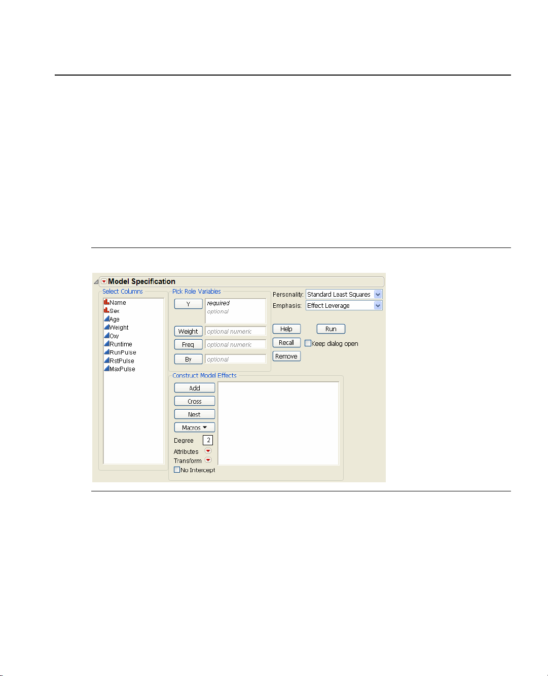
Chapter 1 Introduction to Model Fitting 3

The Fit Model Dialog: A Quick Example

The Fit Model command first displays the Fit Model dialog, shown in Figure 1.1. You use this dialog to tailor a model for your data. The Fit Model dialog is nonmodal, which means it persists until you explicitly close it. This is useful to change the model specification and fit several different models before closing the window.

The example in Figure 1.1, uses the The data are results of an aerobic fitness study. The variable. The variables

Weight, Runtime, RunPulse, RstPulse, and MaxPulse that show in the Construct

Fitness.jmp (SAS Institute 1987) data table in the Sample Data folder.

Oxy variable is a continuous response (dependent)

Model Effects list are continuous effects (also called regressors, factors, or independent variables). The popup menu at the upper-right of the dialog shows

Standard Least Squares, which defines the fitting

method or fitting personality. The various fitting personalities are described later in this chapter.

Figure 1.1 The Fit Model Dialog Completed for a Multiple Regression

This standard least squares example, with a single continuous Y variable and several continuous X variables, specifies a multiple regression.

After a model is defined in the Fit Model dialog, click

Run to perform the analysis and generate a report

window with the appropriate tables and supporting graphics.

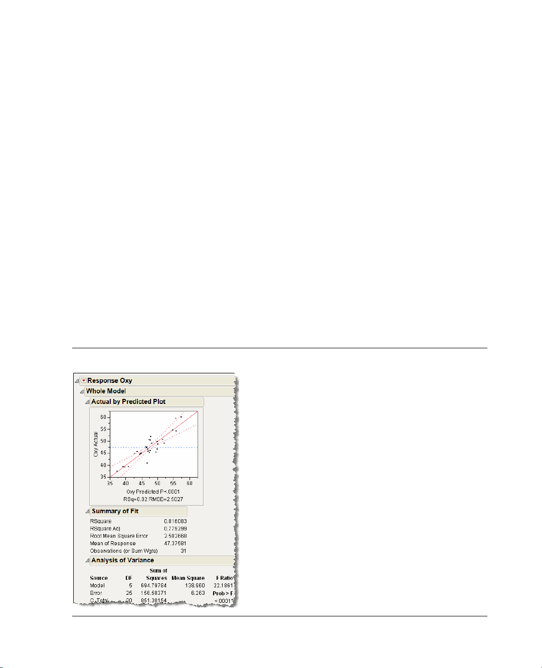
4 Introduction to Model Fitting Chapter 1

The Fit Model Dialog: A Quick Example

A standard least squares analysis such as this multiple regression begins by showing you the Summary of Fit table, the Parameter Estimates table, the Effect Tests table, Analysis of Variance, and the Residual by Predicted and Leverage plots. If you want, you can open additional tables and plots, such as those shown in Figure 1.2, to see details of the analysis. Or, if a screening or response surface analysis seems more appropriate, you can choose commands from the Effect Screening and Factor Profiling menus at the top of the report.

All tables and graphs available on the Fit Model platform are discussed in detail in the chapters “Standard

Least Squares: Introduction,” p. 21, and “Standard Least Squares: Perspectives on the Estimates,” p. 57, and “Standard Least Squares: Exploring the Prediction Equation,” p. 89.

See Table 1.1 “Types of Models,” p. 5, and Table 1.2 “Clicking Sequences for Selected Models,” p. 6, in the next section for a description of models and the clicking sequences needed to enter them into the Fit Model dialog.

Detailed Example of the Fit Model Dialog

1. Open the

2. Select

3. Select

4. Select

5. Click

Figure 1.2 Partial Report for Multiple Regression

Fitness.jmp sample data table.

Analyze > Fit Model.

Oxy and click Y.

Weight, Runtime, RunPulse, RstPulse, and MaxPulse and click Add.

Run.

Chapter 1 Introduction to Model Fitting 5

Types of Models

The list in Table 1.1 “Types of Models,” p. 5 is a catalog of model examples that can be defined using the Fit Model dialog, where the effects X and Z have continuous values, and A, B, and C have nominal or ordinal values. This list is not exhaustive.

When you correctly specify the type of model, the model effects show in the

Construct Model Effects list

on the Fit Model dialog. Refer to Table 1.2 “Clicking Sequences for Selected Models,” p. 6 to see the clicking sequences that produce some of these sets of model effects.

Ta bl e 1 . 1 Types of Models

Type of Model Model Effects

simple regression X

polynomial (x) to Degree 2

X, X*X

polynomial (x, z) to Degree 2 X, X*X, Z, Z*Z

cubic polynomial (x) X, X*X, X*X*X

multiple regression X, Z, …, other continuous columns

one-way analysis of variance A

two-way main effects analysis of

A, B

variance

two-way analysis of variance with

A, B, A*B

interaction

three-way full factorial A, B, A*B, C, A*C, B*C, A*B*C

analysis of covariance, same slopes A, X

analysis of covariance, separate slopes A, X, A*X

simple nested model A, B[A]

compound nested model A, B[A], C[A B]

simple split-plot or repeated measure A, B[A]&Random, C, A*C

response surface (x) model X&RS, X*X

response surface (x, z) model X&RS, Z&RS, X*X, Z*Z, X*Z

MANOVA multiple Y variables

6 Introduction to Model Fitting Chapter 1

Types of Models

The following convention is used to specify clicking:

• If a column name is in plain typeface, click the name in the column selection list.

• If a column name is

bold, then select that column in the dialog model effects list.

• The name of the button to click is shown in all CAPITAL LETTERS.

Ta bl e 1 . 2 Clicking Sequences for Selected Models

Type of Model Clicking Sequence

simple regression X, ADD

polynomial (x) to Degree 2 X,

Degree 2, select Polynomial to Degree in the Macros popup

polynomial (x, z) to Degree 3X, Z,

Degree 3, select Polynomial to Degree in the Macros popup

multiple regression X, ADD, Z, ADD,… or X, Z, …, ADD

one-way analysis of variance A, ADD

two-way main effects

A, ADD B, ADD, or A, B, ADD

analysis of variance

two-way analysis of variance with interaction

three-way full factorial A, B, C, select

analysis of covariance, same

A, B, ADD, A, B, CROSS or

A, B, select

Full Factorial in Macros popup menu

A, ADD, X, ADD or A, X, ADD

slopes

analysis of covariance,

A, ADD, X, ADD, A, X, CROSS

separate slopes

simple nested model A, ADD, B, ADD, A,

A, B, ADD, A,

B, NEST, or

B, NEST

compound nested model A, B, ADD, A,

simple split-plot or repeated measure

two-factor response surface X, Z, select

A, ADD, B, ADD, A,

Attributes

popup menu, C, ADD, C, A, CROSS

Response Surface in the Macros popup menu

B, NEST, C, ADD, A, B, C, NEST

B, NEST, select Random from the Effect

Chapter 1 Introduction to Model Fitting 7

The Response Buttons (Y, Weight, Freq, and By)

The column selection list in the upper left of the dialog lists the columns in the current data table. When you click a column name, it highlights and responds to the action that you choose with other buttons on the dialog. Either drag across columns or Shift-click to extend a selection of column names, and Control-click (-click on the Macintosh) to select non-adjacent names.

To assign variables to the

•

Y identifies one or more response variables (the dependent variables) for the model.

•

Weight is an optional role that identifies one column whose values supply weights for the response.

Y, Weight, Freq, or By roles, select them and click the corresponding role button:

Weighting affects the importance of each row in the model.

•

Freq is an optional role that identifies one column whose values assign a frequency to each row for the

analysis. The values of this variable determine how degrees of freedom are counted.

•

By is used to perform a separate analysis for each level of a classification or grouping variable.

If you want to remove variables from roles, highlight them and click

Construct Model Effects Buttons

Suppose that a data table contains the variables X and Z with continuous values, and A, B, and C with nominal values. The following paragraphs describe the buttons in the Fit Model dialog that specify model effects.

Add

To add a simple regressor (continuous column) or a main effect (nominal or ordinal column) as an x effect to any model, select the column from the column selection list and click in the model effects list. As you add effects, be aware of the modeling type declared for that variable and the consequences that modeling type has when fitting the model:

Remove or hit the backspace key.

Add. That column name appears

• Variables with continuous modeling type become simple regressors.

• Variables with nominal modeling types are represented with dummy variables to fit separate coefficients for each level in the variable.

• Nominal and ordinal modeling types are handled alike, but with a slightly different coding. See the appendix “Statistical Details,” p. 621, for details on coding of effects.

If you mistakenly add an effect, select it in the model effects list and click

Remove.

8 Introduction to Model Fitting Chapter 1

Macros Popup Menu

Cross

To create a compound effect by crossing two or more variables, Shift-click in the column selection list to select them if they are next to each other in the Macintosh) if the variables are not contiguous in the column selection list. Then click

Select Columns list. Control-click (-click on the

Cross:

• Crossed nominal variables become interaction effects.

• Crossed continuous variables become multiplied regressors.

• Crossing a combination of nominal and continuous variables produces special effects suitable for testing homogeneity of slopes.

If you select both a column name in the column selection list and an effect in the model effects list, the

Cross button crosses the selected column with the selected effect and adds this compound effect to the

effects list.

See the appendix “Statistical Details,” p. 621, for a discussion of how crossed effects are parameterized and coded.

Nest

When levels of an effect B only occur within a single level of an effect A, then B is said to be nested within A and A is called the outside effect. The notation B[A] is read “B within A” and means that you want to fit a B effect within each level of A. The B[A] effect is like pooling B and A*B. To specify a nested effect

• select the outside effects in the column selection list and click

• select the nested effect in the column selection list and click

• select the outside effect in the column selection list

• select the nested variable in the model effects list and click

For example, suppose that you want to specify Then click

Cross to see A*B in the model effects list. Highlight the A*B term in the model effects list and C

in the column selection list. Click

Note: The nesting terms must be specified in order, from outer to inner. If B is nested within A, and C is nested within B, then the model is specified as:

JMP allows up to ten terms to be combined as crossed and nested.

Macros Popup Menu

Commands from the Macros popup menu automatically generate the effects for commonly used models. You can add or remove terms from an automatic model specification as needed.

Full Factorial To look at many crossed factors, such as in a factorial design, use Full Factorial. It

creates the set of effects corresponding to all crossings of all variables you select in the columns list. For example, if you select variables A, B, and C, the A*C, B*C, A*B*C in the effect lists. To remove unwanted model interactions, highlight them and click

Remove.

Add or Cross

Nest

A*B[C]. Highlight both A and B in the column selection list.

Nest to see A*B[C] as a model effect.

A, B[A], C[B,A].

Full Factorial selection generates A, B, A*B, C,

Chapter 1 Introduction to Model Fitting 9

β1A β11A

β1A β11A2β2B β22B2β12AB++++

Macros Popup Menu

Factorial to Degree

Degree box, then select Factorial to a Degree.

Factorial Sorted The Factorial Sorted selection creates the same set of effects as Full Factorial but

To create a limited factorial, enter the degree of interactions that you want in the

lists them in order of degree. All main effects are listed first, followed by all two-way interactions, then all three-way interactions, and so forth.

Response Surface In a response surface model, the object is to find the values of the terms that

produce a maximum or minimum expected response. This is done by fitting a collection of terms in a quadratic model. The critical values for the surface are calculated from the parameter estimates and presented with a report on the shape of the surface.

To specify a response surface effect, select two or more variables in the column selection list. When you choose

Response Surface from the Effect Macros popup menu, response surface expressions

appear in the model effects list. For example, if you have variables A and B

Surface(A) fits

Surface(A,B) fits

The response surface effect attribute, prefixed with an ampersand (&), is automatically appended to the effect name in the model effects list. The next section discusses the

Mixture Response Surface The Mixture Response Surface design omits the squared terms and

the intercept and attaches the

&RS effect attribute to the main effects. For more information see the

Attributes popup menu.

Design of Experiments Guide.

Polynomial to Degree A polynomial effect is a series of terms that are powers of one variable. To

specify a polynomial effect:

• click one or more variables in the column selection list;

• enter the degree of the polynomial in the

•use the

For example, suppose you select variable x. A 2 and x

Scheffe Cubic When you fit a 3rd degree polynomial model to a mixture, it turns out that you need

Polynomial to Degree command in the Macros popup menu.

. A 3rd polynomial in the model dialog fits parameters for x, x2, and x3.

Degree box;

polynomial in the effects list fits parameters for x

to take special care not to introduce even-powered terms, because they are not estimable. When you get up to a cubic model, this means that you can't specify an effect like X1*X1*X2. However, it turns out that a complete polynomial specification of the surface should introduce terms of the form:

X1*X2*(X1 – X2)

which we call Scheffe Cubic terms.

In the Fit Model dialog, this macro creates a complete cubic model, including the Scheffe Cubic terms if you either (a) enter a 3 in the Degree box, then do a “Mixture Response Surface” command on a set of mixture columns, or(b) use the

Radial fits a radial-basis smoothing function using the selected variables.

Scheffe Cubic command in the Macro button.

10 Introduction to Model Fitting Chapter 1

Effect Attributes and Transformations

The Attributes popup menu has five special attributes that you can assign to an effect in a model:

Random Effect If you have multiple error terms or random effects, as with a split-plot or repeated

measures design, you can highlight them in the model effects list and select the

Attributes popup menu. See the chapter “Standard Least Squares: Random Effects,” p. 103, for

a detailed discussion and example of random effects.

Response Surface Effect If you have a response surface model, you can use this attribute to identify

which factors participate in the response surface. This attribute is automatically assigned if you use the

Response Surface effects macro. You need only identify the main effects, not the crossed terms,

to obtain the additional analysis done for response surface factors.

Log Variance Effect Sometimes the goal of an experiment is not just to maximize or minimize the

response itself but to aim at a target response and achieve minimum variability. To analyze results from this kind of experiment:

1. Assign the response (Y) variable and choose

Loglinear Variance as the fitting personality

2. Specify loglinear variance effects by highlighting them in the model effects list and select

LogVariance Effect from the Attributes popup menu. The effect appears in the model effects list

with

&LogVariance next to its name.

If you want an effect to be used for both the mean and variance of the response, you must specify it as an effect twice, once with the

Mixture Effect You can use the Mixture Effect attribute to specify a mixture model effect without

using the

Mixture Response Surface effects macro. If you don’t use the effects macro you have to

LogVariance Effect attribute.

add this attribute to the effects yourself so that the model understands which effects are part of the mixture.

Excluded Effect Use the Excluded Effect attribute when you want to estimate least squares means

of an interaction, or include it in lack of fit calculations, but don’t want it in the model.

Knotted Spline Effect Use the Knotted Spline Effect attribute to have JMP fit a segmentation of

smooth polynomials to the specified effect. When you select this attribute, a dialog box appears that allows you to specify the number of knot points.

Note: Knotted splines are only implemented for main-effect continuous terms.

JMP follows the advice in the literature in positioning the points. The knotted spline is also referred to as a Stone spline or a Stone-Koo spline. See Stone and Koo (1986). If there are 100 or fewer points, the first and last knot are the fifth point inside the minimum and maximum, respectively. Otherwise, the first and last knot are placed at the 0.05 and 0.95 quantile if there are 5 or fewer knots, or the 0.025 and 0.975 quantile for more than 5 knots. The default number of knots is 5 unless there are less than or equal to 30 points, in which case the default is 3 knots.

Random Effect from

Knotted splines have the following properties in contrast to smoothing splines:

• Knotted splines work inside of general models with many terms, where smoothing splines are for bivariate regressions.

• The regression basis is not a function of the response.

Chapter 1 Introduction to Model Fitting 11

Effect Attributes and Transformations

• Knotted splines are parsimonious, adding only k – 2 terms for curvature for k knot points.

• Knotted splines are conservative compared to pure polynomials in the sense that the extrapolation outside the range of the data is a straight line, rather than a (curvy) polynomial.

• There is an easy test for curvature.

To test for curvature, select

1. Open the

2. Select

3. Assign

4. Select the

Effect

Growth.jmp sample data table.

Analyze > Fit Model.

ratio to Y and add age as an effect to the model.

age variable in the Construct Model Effects box and select Attributes > Knotted Spline

5. Specify the number of knots as 5, and click

6. Click

Run.

Estimates > Custom Test and add a column for each knotted effect, as follows:

OK.

When the report appears:

7. Select

Estimates > Custom Test and notice that there is only one column. Therefore, click the Add

Column

button twice to produce a total of three columns.

8. Fill in the three knotted columns with ones so that they match Figure 1.3.

Figure 1.3 Construction of Custom Test for Curvature

9. Click Done.

This produces the report shown in Figure 1.4. The low Prob > F value indicates that there is indeed curvature to the data.

12 Introduction to Model Fitting Chapter 1

11605

Temp 273.15+

------------------------------------

Fitting Personalities

Figure 1.4 Curvature Report

Transformations (Standard Least Squares Only)

The Transformations popup menu has eight functions available to transform selected continuous effects or Y columns for standard least squares analyses only. The available transformations are

Square, Reciprocal, Exp, Arrhenius, and ArrheniusInv. These transformations are only supported for

single-column continuous effects.

None, Log, Sqrt,

The Arrhenius transformation is

Fitting Personalities

The Fit Model dialog in JMP serves many different fitting methods. Rather than have a separate dialog for each method, there is one dialog with a choice of fitting personality for each method. Usually the personality is chosen automatically from the context of the response and factors you enter, but you can change selections from the

The following list briefly describes each type of model. Details about text reports, plots, options, special commands, and example analyses are found in the individual chapters for each type of model fit:

Standard Least Squares JMP models one or more continuous responses in the usual way through

fitting a linear model by least squares. The standard least squares report platform offers two flavors of tables and graphs:

Traditional statistics are for situations where the number of error degrees of freedom allows hypothesis testing. These reports include leverage plots, least squares means, contrasts, and output formulas.

Fitting Personality popup menu to alternative methods.

Chapter 1 Introduction to Model Fitting 13

Fitting Personalities

Screening and Response Surface Methodology analyze experimental data where there are many effects but few observations. Traditional statistical approaches focus on the residual error. However, because in near-saturated designs there is little or no room for estimating residuals, the focus is on the prediction equation and the effect sizes. Of the many effects that a screening design can fit, you expect a few important terms to stand out in comparison to the others. Another example is when the goal of the experiment is to optimize settings rather than show statistical significance; the factor combinations that optimize the predicted response are of overriding interest.

Stepwise Stepwise regression is an approach to selecting a subset of effects for a regression model. The

Stepwise feature computes estimates that are the same as those of other least squares platforms, but

it facilitates searching and selecting among many models. The

Stepwise personality allows only one

continuous Y.

Manova When there is more than one Y variable specified for a model with the Manova fitting

personality selected, the Fit Model platform fits the Y’s to the set of specified effects and provides multivariate tests.

LogLinear Variance LogLinear Variance is used when one or more effects model the variance rather

than the mean. The

LogLinear Variance personality must be used with caution. See “Fitting

Dispersion Effects with the LogLinear Variance Model,” p. 155 for more information on this

feature.

Nominal Logistic If the response is nominal, the Fit Model platform fits a linear model to a

multilevel logistic response function using maximum likelihood.

Ordinal Logistic If the response variable has an ordinal modeling type, the Fit Model platform fits the

cumulative response probabilities to the logistic distribution function of a linear model by using maximum likelihood.

Proportional Hazard The proportional hazard (Cox) model is a special fitting personality that lets

you specify models where the response is time-to-failure. The data may include right-censored observations and time-independent covariates. The covariate of interest may be specified as a grouping variable that defines sub populations or strata.

Parametric Survival Parametric Survival performs the same analysis as the Fit Parametric Survival

command on the

Analyze > Reliability and Survival menu. See Quality and Reliability Methods for

details.

Generalized Linear Model fits generalized linear models with various distribution and link

functions. See the chapter “Generalized Linear Models,” p. 197 for a complete discussion of generalized linear models.

Ta bl e 1 . 3 Characteristics of Fitting Personalities

Personality Response (Y) Type Notes

Standard Least Squares ≥ 1 continuous all effect types

Stepwise 1 continuous all effect types

MANOVA > 1 continuous all effect types

LogLinear Variance 1 continuous variance effects

14 Introduction to Model Fitting Chapter 1

Other Model Dialog Features

Ta bl e 1 . 3 Characteristics of Fitting Personalities (Continued)

Personality Response (Y) Type Notes

Nominal Logistic 1 nominal all effect types

Ordinal Logistic 1 ordinal all effect types

Proportional Hazard 1 continuous survival models only

Parametric Survival ≥ 1 continuous survival models only

Generalized Linear Model continuous, nominal, ordinal all effect types

Other Model Dialog Features

Emphasis Choices

The Emphasis popup menu controls the type of plots you see as part of the initial analysis report.

Effect Leverage begins with leverage and residual plots for the whole model. You can then request

effect details and other statistical reports.

Effect Screening shows whole model information followed by a scaled parameter report with graph

and the Prediction Profiler.

Minimal Report suppresses all plots except the regression plot. You request what you want from the

platform popup menu.

Run

The Run button submits the model to the fitting platform. Because the Fit Model dialog is nonmodal, the

Run

button does not close the dialog window. You can continue to use the dialog and make changes to the

model for additional fits. You can also make changes to the data and then refit the same model.

Keep Dialog Open

Checking this option keeps the Model Specification Dialog open after clicking

Validity Checks

Fit Model checks your model for errors such as duplicate effects or missing effects in a hierarchy. If you get

an alert message, you can either message to stop the fitting process.

In addition, your data may have missing values. The default behavior is to exclude rows if any Y or X value is missing. This can be wasteful of rows for cases when some Y’s have non-missing values and other Y’s are missing. Therefore, you may consider fitting each Y separately.

Run.

Continue the fitting despite the situation, or click Cancel in the alert

Chapter 1 Introduction to Model Fitting 15

Other Model Dialog Features

When this situation occurs, you are alerted with a window that asks: “Missing values different across Y columns. Fit each Y separately?” Fitting the Y’s separately uses all non-missing rows for that particular Y. Fitting the Y’s together uses only those rows that are non-missing for both Y’s.

When Y’s are fit separately, the results for the individual analyses are given in a all the Y’s to be profiled in the same Profiler.

Note: This dialog only appears when the model is run interactively. Scripts continue to use the default behavior, unless Fit Separately is placed inside the Run command.

Other Model Specification Options

The popup menu on the title bar of the Model Specification window gives additional options:

Center Polynomials causes a continuous term participating in a crossed term to be centered by its

mean. Exceptions to centering are effects with coded or mixture properties. This option is important to make main effects tests be meaningful hypotheses in the presence of continuous crossed effects.

Set Alpha Level is used to set the alpha level for confidence intervals in the Fit Model analysis.

Save to Data Table saves the model as a property of the current data table. A Model popup menu

icon appears in the Tables panel at the left of the data grid with a select this The JMP Scripting Guide is the reference for JSL statements.

Save to Script window saves the JSL commands for the completed model in a new open script

window. You can save the script window and recreate the model at any time by running the script.

Create SAS job creates a SAS program in a script window that can recreate the current analysis in

SAS. Once created, you have several options for submitting the code to SAS.

1. Copy and Paste the resulting code into the SAS Program Editor. This method is useful if you are running an older version of SAS (pre-version 8.2).

2. Select Edit > Submit to SAS.

Submit to SAS brings up a dialog (shown here) that allows you to enter the machine name and port

of an accessible SAS server (reached through an integrated object model, or IOM), or you can connect directly to SAS on your personal computer. The dialog allows you to enter profiles for any new SAS servers. Results are returned to JMP and are displayed in a separate log window.

Run Script command to submit the model, a new completed Fit Model dialog appears.

Fit Group report. This allows

Run Script command. If you then

16 Introduction to Model Fitting Chapter 1

Formula Editor Model Features

Figure 1.5 Connect to SAS Server Window

3. Save the file and double-click it to open it in a local copy of SAS. This method is useful if you would like to take advantage of SAS ODS options, e.g. generating HTML or PDF output from the SAS code.

Load Version 3 Model presents an Open File dialog for you to select a text file that contains JMP

Version 3 model statements. The model then appears in the Fit Model dialog, and can be saved as a current-version model.

Formula Editor Model Features

There are several features in the Formula Editor that are useful for constructing models.

Parametric Models

In the Functions List, the Parametric Model group is useful in creating linear regression components. Each presents a dialog that allows you to select the columns involved in the model.

Chapter 1 Introduction to Model Fitting 17

Formula Editor Model Features

Figure 1.6 Parametric Model Group

Linear Model builds a linear model, with a parameter as the coefficient as each term.

Examples of Parametric Models

1. Open the

2. Double-click in the empty column after

3. Right-click on the

4. Scroll down to the bottom of the Function list, and select

5. Select the following columns:

Odor Control Original.jmp sample data table.

odor to create a new column. Name the column Linear Model.

Linear Model column and select Formula.

Parametric Model > Linear Model.

temp, gl ratio, and ht, and click OK.

Figure 1.7 shows the resulting linear model formula.

Figure 1.7 Linear Model Formula

18 Introduction to Model Fitting Chapter 1

Formula Editor Model Features

Interactions Model

6. Select

Parametric Model > Interactions Model.

7. Select the following columns:

builds a linear model with first-order interactions:

temp, gl ratio, and ht, and click OK.

Figure 1.8 shows the resulting interactions model formula.

Figure 1.8 Interactions Model Formula

Full Quadratic Model builds a model with linear, first-order interaction, and quadratic terms.

8. Select

9. Select the following columns:

Parametric Model > Full Quadratic Model.

temp, gl ratio, and ht, and click OK.

Figure 1.8 shows the resulting full quadratic model formula.

Figure 1.9 Full Quadratic Model Formula

Chapter 1 Introduction to Model Fitting 19

Formula Editor Model Features

Adding Parameters

When adding a parameter to a model in the Formula Editor, the Expand into categories checkbox is useful for making parametric expressions across categories.

Example of Adding a Parameter

1. Open the

Odor Control Original.jmp sample data table.

Add a parameter for each level of the

2. Right-click on the

3. Click on the arrow next to

4. Select

New Parameter.

5. Keep the parameter name

6. Next to value, type

7. Select

8. Select

Expand into categories, selecting columns and click OK.

temp and click OK.

9. Click on the new parameter,

Figure 1.10 New Parameter

temp column and select Formula.

Tabl e Colu m ns and select Parameters.

b0.

tempParam.

b0_temp = “tempParam”.

temp variable:

This formula creates new parameters named b0_temp_n for each level of temp.

20 Introduction to Model Fitting Chapter 1

Formula Editor Model Features

Chapter 2

Standard Least Squares: Introduction

The Fit Model Platform

The Fit Model platform contains the Standard Least Squares personality. This fitting facility can fit many different types of models (regression, analysis of variance, analysis of covariance, and mixed models), and you can explore the fit in many ways. Even though this is a sophisticated platform, you can do simple tasks very easily.

This Standard Least Squares fitting personality is used for a continuous-response fit to a linear model of factors using least squares. The results are presented in detail, and include leverage plots and least squares means. There are many additional features to consider, such as making contrasts and saving output formulas. More detailed discussions of the Standard Least Squares fitting personality are included in other chapters.

• If you haven’t learned how to specify your model in the Model Specification window, you can refer to the chapter “Introduction to Model Fitting,” p. 1.

• If you have response surface effects or want retrospective power calculations, see the chapter “Standard

Least Squares: Perspectives on the Estimates,” p. 57.

• For screening applications, see the chapter “Standard Least Squares:

Exploring the Prediction Equation,” p. 89.

• If you have random effects, see the chapter “Standard Least Squares: Random Effects,” p. 103.

• If you need the details on how JMP parameterizes its models, see the appendix “Statistical Details,”

p. 621.

The Standard Least Squares Personality is just one of many fitting personalities of the Fit Model platform. The other eight personalities are covered in the later chapters “Standard Least Squares:

Perspectives on the Estimates,” p. 57, “Standard Least Squares: Exploring the Prediction Equation,” p. 89, “Standard Least Squares: Random Effects,” p. 103, “Generalized Linear Models,” p. 197, “Fitting Dispersion Effects with the LogLinear Variance Model,” p. 155, “Stepwise Regression,” p. 117, and “Logistic Regression for Nominal and Ordinal Response,” p. 165, and “Multiple Response Fitting,” p. 135.

Contents

Launch the Platform: A Simple Example. . . . . . . . . . . . . . . . . . . . . . . . . . . . . . . . . . . . . . . . . . . . . . . . . .23

Regression Plot . . . . . . . . . . . . . . . . . . . . . . . . . . . . . . . . . . . . . . . . . . . . . . . . . . . . . . . . . . . . . . . . . 26

Option Packages for Emphasis. . . . . . . . . . . . . . . . . . . . . . . . . . . . . . . . . . . . . . . . . . . . . . . . . . . . . . . . . 27

Whole-Model Statistical Tables . . . . . . . . . . . . . . . . . . . . . . . . . . . . . . . . . . . . . . . . . . . . . . . . . . . . . . . . .28

The Summary of Fit Table. . . . . . . . . . . . . . . . . . . . . . . . . . . . . . . . . . . . . . . . . . . . . . . . . . . . . . . . . .28

The Analysis of Variance Table . . . . . . . . . . . . . . . . . . . . . . . . . . . . . . . . . . . . . . . . . . . . . . . . . . . . . 30

The Lack of Fit Table . . . . . . . . . . . . . . . . . . . . . . . . . . . . . . . . . . . . . . . . . . . . . . . . . . . . . . . . . . . . . 31

The Parameter Estimates Table . . . . . . . . . . . . . . . . . . . . . . . . . . . . . . . . . . . . . . . . . . . . . . . . . . . . . .33

The Effect Test Table. . . . . . . . . . . . . . . . . . . . . . . . . . . . . . . . . . . . . . . . . . . . . . . . . . . . . . . . . . . . . .34

Saturated Models. . . . . . . . . . . . . . . . . . . . . . . . . . . . . . . . . . . . . . . . . . . . . . . . . . . . . . . . . . . . . . . . . . . . 35

Leverage Plots . . . . . . . . . . . . . . . . . . . . . . . . . . . . . . . . . . . . . . . . . . . . . . . . . . . . . . . . . . . . . . . . . . . . . .36

Effect Details. . . . . . . . . . . . . . . . . . . . . . . . . . . . . . . . . . . . . . . . . . . . . . . . . . . . . . . . . . . . . . . . . . . . . . 40

LSMeans Table . . . . . . . . . . . . . . . . . . . . . . . . . . . . . . . . . . . . . . . . . . . . . . . . . . . . . . . . . . . . . . . . . 40

LSMeans Plot . . . . . . . . . . . . . . . . . . . . . . . . . . . . . . . . . . . . . . . . . . . . . . . . . . . . . . . . . . . . . . . . . . .41

LSMeans Contrast. . . . . . . . . . . . . . . . . . . . . . . . . . . . . . . . . . . . . . . . . . . . . . . . . . . . . . . . . . . . . . . .43

LSMeans Student’s t, LSMeans Tukey’s HSD . . . . . . . . . . . . . . . . . . . . . . . . . . . . . . . . . . . . . . . . . . .45

Test S l i c e s . . . . . . . . . . . . . . . . . . . . . . . . . . . . . . . . . . . . . . . . . . . . . . . . . . . . . . . . . . . . . . . . . . . . . 46

Power Analysis . . . . . . . . . . . . . . . . . . . . . . . . . . . . . . . . . . . . . . . . . . . . . . . . . . . . . . . . . . . . . . . . . . 46

Summary of Row Diagnostics and Save Commands . . . . . . . . . . . . . . . . . . . . . . . . . . . . . . . . . . . . . . . . 46

Row Diagnostics . . . . . . . . . . . . . . . . . . . . . . . . . . . . . . . . . . . . . . . . . . . . . . . . . . . . . . . . . . . . . . . . 47

Save Columns Command . . . . . . . . . . . . . . . . . . . . . . . . . . . . . . . . . . . . . . . . . . . . . . . . . . . . . . . . . 48

Examples with Statistical Details . . . . . . . . . . . . . . . . . . . . . . . . . . . . . . . . . . . . . . . . . . . . . . . . . . . . . . . 49

One-Way Analysis of Variance with Contrasts . . . . . . . . . . . . . . . . . . . . . . . . . . . . . . . . . . . . . . . . . . 50

Analysis of Covariance. . . . . . . . . . . . . . . . . . . . . . . . . . . . . . . . . . . . . . . . . . . . . . . . . . . . . . . . . . . . .52

Analysis of Covariance with Separate Slopes . . . . . . . . . . . . . . . . . . . . . . . . . . . . . . . . . . . . . . . . . . . .54

Singularity Details . . . . . . . . . . . . . . . . . . . . . . . . . . . . . . . . . . . . . . . . . . . . . . . . . . . . . . . . . . . . . . . . . . .56

Chapter 2 Standard Least Squares: Introduction 23

Launch the Platform: A Simple Example

To introduce the Fit Model platform, consider a simple one-way analysis of variance to test if there is a difference in the mean response among three drugs. The example data (Snedecor and Cochran 1967) is a study that measured the response of 30 subjects after treatment by each of three drugs labeled The results are in the

Drug.jmp sample data table.

a, d, and f.

1. Open the

2. Select

Drug.jmp sample data table.

Analyze > Fit Model.

See the chapter “Introduction to Model Fitting,” p. 1, for details about how to use this window.

3. Select

4. Select

Figure 2.1 The Fit Model Window For a One-Way Analysis of Variance

y and click Y.

When you select the column

Squares

and the Emphasis is Effect Leverage. You can change these options in other situations.

Drug and click Add.

y to be the Y response, the Fitting Personality becomes Standard Least

5. Click Run.

At the top of the output are the graphs in Figure 2.2 that show how the data fit the model. These graphs are called leverage plots, because they convey the idea of the data points pulling on the lines representing the fitted model. Leverage plots have these useful properties:

• The distance from each point to the line of fit is the error or residual for that point.

24 Standard Least Squares: Introduction Chapter 2

Launch the Platform: A Simple Example

• The distance from each point to the horizontal line is what the error would be if you took out effects in the model.

Thus, strength of the effect is shown by how strongly the line of fit is suspended away from the horizontal by the points. Confidence curves are on the graph so you can see at a glance whether an effect is significant. In each plot, if the 95% confidence curves cross the horizontal reference line, then the effect is significant. If the curves do not cross, then it is not significant (at the 5% level).

Figure 2.2 Whole Model Leverage Plot and Drug Effect Leverage Plot

In this simple case where predicted values are simple means, the leverage plot for Drug shows a regression of the actual values on the means for the drug level. Levin, Serlin, and Webne-Behrman (1989) showcase this idea.

Because there is only one effect in the model, the leverage plot for Whole Model and for the effect

Drug are

equivalent. They differ only in the scaling of the x-axis. The leverage plot for the Whole Model is a plot of the actual response versus the predicted response. So, the points that fall on the line are those that are perfectly predicted.

In this example, the confidence curve does cross the horizontal line. Thus, the drug effect is marginally significant, even though there is considerable variation around the line of fit (in this case around the group means).

After you examine the fit graphically, you can look below it for textual details. In this case there are three levels of

Drug, giving two parameters to characterize the differences among them. Text reports show the

estimates and various test statistics and summary statistics concerning the parameter estimates. The Summary of Fit table and the Analysis of Variance table beneath the whole-model leverage plot show the fit as a whole. Because

Drug is the only effect, the same test statistic appears in the Analysis of Variance table

and in the Effects Tests table. Results for the Summary of Fit and the Analysis of Variance are shown in Figure 2.3.

Chapter 2 Standard Least Squares: Introduction 25

Launch the Platform: A Simple Example

Figure 2.3 Summary of Fit and Analysis of Variance

The Analysis of Variance table shows that the Drug effect has an observed significance probability (Prob > F) of 0.0305, which is significant at a 0.05 level. The RSquare value means that 22.8% of the variation in the response can be absorbed by fitting this model.

Whenever there are nominal effects (such as

Drug), it is interesting to compare how well the levels predict

the response. Rather than use the parameter estimates directly, it is usually more meaningful to compare the predicted values at the levels of the nominal values. These predicted values are called the least squares means (LSMeans), and in this simple case, they are the same as the ordinary means. Least squares means can differ from simple means when there are other effects in the model, as seen in later examples. The Least Squares Means table for a nominal effect shows beneath the effect’s leverage plot (Figure 2.4).

The popup menu for an effect also lets you request the

LSMeans Plot, as shown in Figure 2.4. The plot

graphically shows the means and their associated 95% confidence interval.

26 Standard Least Squares: Introduction Chapter 2

Launch the Platform: A Simple Example

Figure 2.4 Table of Least Squares Means and LS Means Plot

The later section “Examples with Statistical Details,” p. 49, continues the drug analysis with the Parameter Estimates table and looks at the group means with the

Regression Plot

If there is exactly one continuous term in a model, and no more than one categorical term, then JMP plots the regression line (or lines). The regression plot for the drug data is shown in Figure 2.5 and is done as follows:

• Specify the model as in “Launch the Platform: A Simple Example,” p. 23 but this time, add as a model effect.

• The Regression Plot appears by default. You can elect to not show this plot in the output by selecting

Response y in the title bar > Row Diagnostics > Plot Regression. Selecting this command turns the

plot off and on.

LSMeans Contrast.

x with Drug

Chapter 2 Standard Least Squares: Introduction 27

Option Packages for Emphasis

Figure 2.5 Regression Plot

Option Packages for Emphasis

The model fitting process can produce a wide variety of tables, plots, and graphs. For convenience, three standard option packages let you choose the report layout that best corresponds to your needs. Just as automobiles are made available with luxury, sport, and economy option packages, linear model results are made available in choices to adapt to your situation. Table 2.1 “Standard Least Squares Report Layout

Defined by Emphasis,” p. 27, describes the types of report layout for the standard least squares analysis.

The chapter “Introduction to Model Fitting,” p. 1, introduces the

Emphasis is based on the number of effects that you specify and the number of rows (observations) in the

Emphasis menu. The default value of

data table. The Emphasis menu options are summarized in Table 2.1.

Ta bl e 2 . 1 Standard Least Squares Report Layout Defined by Emphasis

Emphasis Description of Reports

Effect Leverage Choose Effect Leverage when you want details on the significance of each

effect. The initial reports for this emphasis features leverage plots, and the reports for each effect are arranged horizontally.

Effect Screening

The

Effect Screening layout is better when you have many effects, and

don’t want details until you see which effects are stronger and which are weaker. This is the recommended method for screening designs, where there are many effects and few observations, and the quest is to find the strong effects, rather than to test significance. This arrangement initially displays whole model information followed by effect details, scaled estimates, and the prediction profiler.

Minimal Report

Minimal Report starts simple; you customize the results with the tables and

plots you want to see. Choosing

Minimal Report suppresses all plots

(except the regression plot), and arranges whole model and effect detail tables vertically.

28 Standard Least Squares: Introduction Chapter 2

Whole-Model Statistical Tables

This section starts the details on the standard statistics inside the reports. You might want to skim some of these details sections and come back to them later.

Regression reports can be turned on and off with the Regression Reports menu. This menu, shown in Figure 2.6, is accessible from the report’s red triangle menu.

Figure 2.6 Regression Report Options

The Whole Model section shows how the model fits as a whole. The next sections describe these tables:

• Summary of Fit

• Analysis of Variance

•Lack of Fit

• Parameter Estimates

•Effect Tests

Discussion of tables for effects and leverage plots are described under the sections “The Effect Test Table,”

p. 34, and “Leverage Plots,” p. 36.

The

Show All Confidence Intervals command shows confidence intervals for parameter estimates in the

Parameter Estimates report, and also for least squares means in Least Squares Means Tables. The command shows AICc and BIC in the Summary of Fit report.

The following examples use the the response variable (Y) and

The Summary of Fit Table

The Summary of Fit table appears first. The numeric summaries of the response for the multiple regression model are shown in Figure 2.7.

AICc

Drug.jmp data table from the Sample Data folder. The model specifies y as

Drug and x as effects, where Drug has the nominal modeling type.

Chapter 2 Standard Least Squares: Introduction 29

Sum of Squares(Model)

Mean Square(Error)

Mean Square(C. Total)

----------------------------------------------------- -

–

Whole-Model Statistical Tables

Figure 2.7 Summary of Fit

The Summary of Fit for the response includes:

RSquare estimates the proportion of the variation in the response around the mean that can be

attributed to terms in the model rather than to random error. Using quantities from the corresponding Analysis of Variance table, R

is calculated:

It is also the square of the correlation between the actual and predicted response. An R when there is a perfect fit (the errors are all zero). An R

of 0 means that the fit predicts the response

of 1 occurs

no better than the overall response mean.

Rsquare Adj adjusts R

to make it more comparable over models with different numbers of parameters by using the degrees of freedom in its computation. It is a ratio of mean squares instead of sums of squares and is calculated

where mean square for

Analysis of Variance Table,” p. 30) and the mean square for

C. Total sum of squares divided by its respective degrees of freedom.

Root Mean Square Error estimates the standard deviation of the random error. It is the square root

Error is found in the Analysis of Variance table (shown next under “The

C. Total can be computed as the

of the mean square for error in the corresponding Analysis of Variance table, and it is commonly denoted as s.

Mean of Response is the overall mean of the response values. It is important as a base model for

prediction because all other models are compared to it. The variance measured around this mean is the Sum of Squares Corrected Total (

Observations (or Sum of Weights) records the number of observations used in the fit. If there are

C. Total) in the Analysis of Variance table.

no missing values and no excluded rows, this is the same as the number of rows in the data table. If there is a column assigned to the role of weight, this is the sum of the weight column values.

30 Standard Least Squares: Introduction Chapter 2

Whole-Model Statistical Tables

The Analysis of Variance Table

The Analysis of Variance table is displayed in Figure 2.8 and shows the basic calculations for a linear model.

Figure 2.8 Analysis of Variance Table

The table compares the model fit to a simple fit of a single mean:

Source lists the three sources of variation, called Model, Error, and C. Total (Corrected Total).

DF records an associated degrees of freedom (DF) for each source of variation.

The

C. Total degrees of freedom is shown for the simple mean model. There is only one degree of

freedom used (the estimate of the mean parameter) in the calculation of variation so the is always one less than the number of observations.

The total degrees of freedom are partitioned into the

The

Model degrees of freedom shown is the number of parameters (except for the intercept) used to

Model and Error terms:

fit the model.

The

Error DF is the difference between the C. Total DF and the Model DF.

Sum of Squares records an associated sum of squares (SS for short) for each source of variation. The

SS column accounts for the variability measured in the response. It is the sum of squares of the differences between the fitted response and the actual response.

The total (

C. Total) SS is the sum of squared distances of each response from the sample mean,

which is 1288.7 in the example shown at the beginning of this section. That is the base model (or simple mean model) used for comparison with all other models.

The

Error SS is the sum of squared differences between the fitted values and the actual values, and is

417.2 in the previous example. This sum of squares corresponds to the unexplained after fitting the regression model.

The total SS less the error SS gives the sum of squares attributed to the

Model.

One common set of notations for these is SSR, SSE, and SST for sum of squares due to regression (model), error, and total, respectively.

Mean Square is a sum of squares divided by its associated degrees of freedom. This computation

converts the sum of squares to an average (mean square).

The

Model mean square is 290.5 in the table at the beginning of this section.

The

Error Mean Square is 16.046 and estimates the variance of the error term. It is often denoted as

MSE or s

C. Total DF

Error (residual)

Chapter 2 Standard Least Squares: Introduction 31

Whole-Model Statistical Tables

F Ratio

is the model mean square divided by the error mean square. It tests the hypothesis that all the regression parameters (except the intercept) are zero. Under this whole-model hypothesis, the two mean squares have the same expectation. If the random errors are normal, then under this hypothesis the values reported in the SS column are two independent Chi-squares. The ratio of these two Chi-squares divided by their respective degrees of freedom (reported in the DF column) has an F-distribution. If there is a significant effect in the model, the chance alone.

Prob > F is the probability of obtaining a greater F-value by chance alone if the specified model fits

no better than the overall response mean. Significance probabilities of 0.05 or less are often considered evidence that there is at least one significant regression factor in the model.

Note that large values of p values. (This is desired if the goal is to declare that terms in the model are significantly different from zero.) Most practitioners check this F-test first and make sure that it is significant before delving further into the details of the fit. This significance is also shown graphically by the whole-model leverage plot described in the previous section.

The Lack of Fit Table

The Lack of Fit table in Figure 2.9 shows a special diagnostic test and appears only when the data and the model provide the opportunity.

Figure 2.9 Lack of Fit Table

F Ratio is higher than expected by

Model SS, relative to small values of Error SS, lead to large F-ratios and low

The idea is that sometimes you can estimate the error variance independently of whether you have the right form of the model. This occurs when observations are exact replicates of each other in terms of the X variables. The error that you can measure for these exact replicates is called pure error. This is the portion of the sample error that cannot be explained or predicted by the form that the model uses for the X variables. However, a lack of fit test is not very useful if it has only a few degrees of freedom (not many replicated x values).

The difference between the residual error from the model and the pure error is called lack of fit error. A lack of fit error can be significantly greater than pure error if you have the wrong functional form of a regressor, or if you do not have enough interaction effects in an analysis of variance model. In that case, you should consider adding interaction terms, if appropriate, or try to better capture the functional form of a regressor.

There are two common situations where there is no lack of fit test:

1. There are no exactly replicated points with respect to the X data, and therefore there are no degrees of

freedom for pure error.

32 Standard Least Squares: Introduction Chapter 2

ni1–()

i 1=



i 1=



Whole-Model Statistical Tables

2. The model is saturated, meaning that the model itself has a degree of freedom for each different x value.

Therefore, there are no degrees of freedom for lack of fit.

The Lack of Fit table shows information about the error terms:

Source lists the three sources of variation called Lack of Fit, Pure Error, and Total Error.

DF records an associated degrees of freedom (DF) for each source of error.

The Total Error DF is the degrees of freedom found on the Error line of the Analysis of Variance table. It is the difference between the Total DF and the Model DF found in that table. The Error DF is partitioned into degrees of freedom for lack of fit and for pure error.

The Pure Error each effect. For example, in the sample data, have the same values of

DF is pooled from each group where there are multiple rows with the same values for

Big Class.jmp, there is one instance where two subjects

age and weight (Chris and Alfred are both 14 and have a weight of 99). This

gives 1(2 - 1) = 1 DF for Pure Error. In general, if there are g groups having multiple rows with identical values for each effect, the pooled DF, denoted DF

where n

is the number of replicates in the ith group.

The Lack of Fit DF is the difference between the Total Error and Pure Error degrees of freedom.

Sum of Squares records an associated sum of squares (SS for short) for each source of error.

The Total Error SS is the sum of squares found on the

Error line of the corresponding Analysis of

Variance table.

The Pure Error SS is pooled from each group where there are multiple rows with the same values for each effect. This estimates the portion of the true random error that is not explained by model effects. In general, if there are g groups having multiple rows with like values for each effect, the pooled SS, denoted SS

where SS

is the sum of squares for the ith group corrected for its mean.

is written

The Lack of Fit SS is the difference between the Total Error and Pure Error sum of squares. If the lack of fit SS is large, it is possible that the model is not appropriate for the data. The F-ratio described below tests whether the variation due to lack of fit is small enough to be accepted as a negligible portion of the pure error.

Mean Square is a sum of squares divided by its associated degrees of freedom. This computation

converts the sum of squares to an average (mean square). F-ratios for statistical tests are the ratios of mean squares.

F Ratio is the ratio of mean square for Lack of Fit to mean square for Pure Error. It tests the hypothesis

that the lack of fit error is zero.

Chapter 2 Standard Least Squares: Introduction 33

SS(Pure Error)

SS(Total for whole model)

-------------------------------------------------------------

–

Whole-Model Statistical Tables

Prob > F

is the probability of obtaining a greater F-value by chance alone if the variation due to lack

of fit variance and the pure error variance are the same. This means that an insignificant proportion of error is explained by lack of fit.

Max RSq is the maximum R

Because Pure Error is invariant to the form of the model and is the minimum possible variance, Max RSq is calculated

The Parameter Estimates Table

The Parameter Estimates table shows the estimates of the parameters in the linear model and a t-test for the hypothesis that each parameter is zero. Simple continuous regressors have only one parameter. Models with complex classification effects have a parameter for each anticipated degree of freedom. The Parameters Estimates table is shown in Figure 2.10.

Figure 2.10 Parameter Estimates Table

that can be achieved by a model using only the variables in the model.

The Parameter Estimates table shows these quantities:

Te rm names the estimated parameter. The first parameter is always the intercept. Simple regressors

show as the name of the data table column. Regressors that are dummy indicator variables constructed from nominal or ordinal effects are labeled with the names of the levels in brackets. For nominal variables, the dummy variables are coded as 1 except for the last level, which is coded as –1 across all the other dummy variables for that effect. The parameters for ordinally coded indicators measure the difference from each level to the level before it. See “Interpretation of Parameters,” p. 627 in the “Statistical Details” chapter, for additional information.

Estimate lists the parameter estimates for each term. They are the coefficients of the linear model

found by least squares.

Std Error is the standard error, an estimate of the standard deviation of the distribution of the

parameter estimate. It is used to construct t-tests and confidence intervals for the parameter.

t Ratio is a statistic that tests whether the true parameter is zero. It is the ratio of the estimate to its

standard error and has a Student’s t-distribution under the hypothesis, given the usual assumptions about the model.

Prob > |t| is the probability of getting an even greater t-statistic (in absolute value), given the

hypothesis that the parameter is zero. This is the two-tailed test against the alternatives in each

34 Standard Least Squares: Introduction Chapter 2

VIF

1 R

–

-------------- -

diag X 'X()

1–

Whole-Model Statistical Tables

direction. Probabilities less than 0.05 are often considered as significant evidence that the parameter is not zero.

Although initially hidden, the following columns are also available. Right-click (control-click on the Macintosh) and select the desired column from the

Columns menu. Alternatively, there is a preference that

can be set to always show the columns.

Std Beta are the parameter estimates that would have resulted from the regression had all the variables

been standardized to a mean of 0 and a variance of 1.

VIF shows the variance inflation factors. High VIFs indicate a collinearity problem.

Note that the VIF is defined as

where R

2 is the coefficient of multiple determination for the regression of xi as a function of the

other explanatory variables.

Note that the definition of R hidden-intercept models, R rather than the corrected sum of squares from the mean model.

Lower 95% is the lower 95% confidence interval for the parameter estimate.

Upper 95% is the upper 95% confidence interval for the parameter estimate.

Design Std Error is the standard error without being scaled by sigma (RMSE), and is equal to

The Effect Test Table

The effect tests are joint tests that all the parameters for an individual effect are zero. If an effect has only one parameter, as with simple regressors, then the tests are no different from the t-tests in the Parameter Estimates table. Parameterization and handling of singularities are different from the SAS GLM procedure. For details, see the appendix “Statistical Details,” p. 621. The Effect Tests table is shown in Figure 2.11.

Figure 2.11 Effect Tests Table

changes for no-intercept models. For no-intercept and

from the uncorrected Sum of Squares or from the zero model is used,

The Effect Tests table shows the following information for each effect:

Source lists the names of the effects in the model.

Chapter 2 Standard Least Squares: Introduction 35

Pseudo t

estimate

relative std error PSE×

----------------------------------------------------- -

Saturated Models

Nparm

is the number of parameters associated with the effect. Continuous effects have one parameter. Nominal effects have one less parameter than the number of levels. Crossed effects multiply the number of parameters for each term. Nested effects depend on how levels occur.

DF is the degrees of freedom for the effect test. Ordinarily Nparm and DF are the same. They are

different if there are linear combinations found among the regressors such that an effect cannot be tested to its fullest extent. Sometimes the DF is zero, indicating that no part of the effect is testable. Whenever DF is less than Nparm, the note

Sum of Squares is the sum of squares for the hypothesis that the listed effect is zero.

F Ratio is the F-statistic for testing that the effect is zero. It is the ratio of the mean square for the

effect divided by the mean square for error. The mean square for the effect is the sum of squares for the effect divided by its degrees of freedom.

Prob > F is the significance probability for the F-ratio. It is the probability that if the null hypothesis

is true, a larger F-statistic would occur only due to random error. Values less than 0.0005 appear as <.0001, which is conceptually zero.

Although initially hidden, a column that displays the Mean Square is also available. Right-click (control-click on the Macintosh) and select

Saturated Models

Screening experiments often involve fully saturated models, where there are not enough degrees of freedom to estimate error. Because of this, neither standard errors for the estimates, nor t-ratios, nor p-values can be calculated in the traditional way.

Lost DFs appears to the right of the line in the report.

Mean Square from the Columns menu.

For these cases, JMP uses the relative standard error, corresponding to a residual standard error of 1. In cases where all the variables are identically coded (say, [–1,1] for low and high levels), these relative standard errors are identical.

JMP also displays a Pseudo-t-ratio, calculated as

using Lenth’s PSE (pseudo standard-error) and degrees of freedom for error (DFE) equal to one-third the number of parameters. The value for Lenth’s PSE is shown at the bottom of the report.

Example of a Saturated Model

1. Open the

2. Select

3. Select

4. Select the following five columns:

5. Click on the

6. Click

Reactor.jmp sample data table.

Analyze > Fit Model.

Y and click Y.

F, Ct, A, T and Cn.

Macros button and select Full Factorial.

Run.

36 Standard Least Squares: Introduction Chapter 2

Leverage Plots

The parameter estimates are presented in sorted order, with smallest p-values listed first. The sorted parameter estimates are presented in Figure 2.12.

Figure 2.12 Saturated Report

In cases where the relative standard errors are different (perhaps due to unequal scaling), a similar report appears. However, there is a different value for Lenth’s PSE for each estimate.

Leverage Plots

To graphically view the significance of the model or focus attention on whether an effect is significant, you want to display the data by focusing on the hypothesis for that effect. You might say that you want more of an X-ray picture showing the inside of the data rather than a surface view from the outside. The leverage plot gives this view of your data; it offers maximum insight into how the fit carries the data.

Chapter 2 Standard Least Squares: Introduction 37

Leverage Plots

The effect in a model is tested for significance by comparing the sum of squared residuals to the sum of squared residuals of the model with that effect removed. Residual errors that are much smaller when the effect is included in the model confirm that the effect is a significant contribution to the fit.

The graphical display of an effect’s significance test is called a leverage plot. See Sall (1990). This type of plot shows for each point what the residual would be both with and without that effect in the model. Leverage plots are found in the

Figure 2.13 Row Diagnostics Submenu

Row Diagnostics submenu, shown in Figure 2.13 of the Fit Model report.

A leverage plot is constructed as illustrated in Figure 2.14. The distance from a point to the line of fit shows the actual residual. The distance from the point to the horizontal line of the mean shows what the residual error would be without the effect in the model. In other words, the mean line in this leverage plot represents the model where the hypothesized value of the parameter (effect) is constrained to zero.

Historically, leverage plots are referred to as a partial-regression residual leverage plot by Belsley, Kuh, and Welsch (1980) or an added variable plot by Cook and Weisberg (1982).

The term leverage is used because a point exerts more influence on the fit if it is farther away from the middle of the plot in the horizontal direction. At the extremes, the differences of the residuals before and after being constrained by the hypothesis are greater and contribute a larger part of the sums of squares for that effect’s hypothesis test.

The fitting platform produces a leverage plot for each effect in the model. In addition, there is one special leverage plot titled Whole Model that shows the actual values of the response plotted against the predicted values. This Whole Model leverage plot dramatizes the test that all the parameters (except intercepts) in the model are zero. The same test is reported in the Analysis of Variance report.

38 Standard Least Squares: Introduction Chapter 2

residual constrained by hypothesis

residual

points farther out pull on the line of fit with greater leverage than the points near the middle

Leverage Plots

Figure 2.14 Illustration of a General Leverage Plot

The leverage plot for the linear effect in a simple regression is the same as the traditional plot of actual response values and the regressor.

Example of a Leverage Plot for a Linear Effect

1. Open the

2. Select

3. Select

4. Select

5. Click

Figure 2.15 Whole Model and Effect Leverage Plots

Big Class.jmp sample data table.

Analyze > Fit Model.

height and click Y.

age and click Add.

Run.

The plot on the left is the Whole Model test for all effects, and the plot on the right is the leverage plot for the effect

age.

Chapter 2 Standard Least Squares: Introduction 39

Significant Borderline Not Significant

confidence curve crosses horizontal line

confidence curve asymptotic to horizontal line

confidence curve does not cross horizontal line

Leverage Plots

The points on a leverage plot for simple regression are actual data coordinates, and the horizontal line for the constrained model is the sample mean of the response. But when the leverage plot is for one of multiple effects, the points are no longer actual data values. The horizontal line then represents a partially constrained model instead of a model fully constrained to one mean value. However, the intuitive interpretation of the plot is the same whether for simple or multiple regression. The idea is to judge if the line of fit on the effect’s leverage plot carries the points significantly better than does the horizontal line.

Figure 2.14 is a general diagram of the plots in Figure 2.15. Recall that the distance from a point to the line of fit is the actual residual and that the distance from the point to the mean is the residual error if the regressor is removed from the model.

Confidence Curves

The leverage plots are shown with confidence curves. These indicate whether the test is significant at the 5% level by showing a confidence region for the line of fit. If the confidence region between the curves contains the horizontal line, then the effect is not significant. If the curves cross the line, the effect is significant. Compare the examples shown in Figure 2.16.

Figure 2.16 Comparison of Significance Shown in Leverage Plots

Interpretation of X Scales

If the modeling type of the regressor is continuous, then the x-axis is scaled like the regressor and the slope of the line of fit in the leverage plot is the parameter estimate for the regressor. (See the left illustration in Figure 2.17.)

If the effect is nominal or ordinal, or if a complex effect like an interaction is present instead of a simple regressor, then the x-axis cannot represent the values of the effect directly. In this case the x-axis is scaled like the y-axis, and the line of fit is a diagonal with a slope of 1. The whole model leverage plot is a version of this. The x-axis turns out to be the predicted response of the whole model, as illustrated by the right-hand plot in Figure 2.17.

40 Standard Least Squares: Introduction Chapter 2

{

residual

residual to the mean

residual

residual to the mean

45 degree line

Effect Details

Figure 2.17 Leverage Plots for Simple Regression and Complex Effects

The influential points in all leverage plots are the ones far out on the x-axis. If two effects in a model are closely related, then these effects as a whole don’t have much leverage. This problem is called collinearity. By scaling regressor axes by their original values, collinearity is shown by shrinkage of the points in the x direction.

See the appendix “Statistical Details,” p. 621, for the details of leverage plot construction.

Effect Details

Each effect has the popup menu shown Figure 2.18 next to its name. The effect popup menu items let you request tables, plots, and tests for that effect. The commands for an effect append results to the effect report. You can close results or dismiss the results by deselecting the item in the menu.

Figure 2.18 Effect Submenu

The next sections describe the Effect popup menu commands.

LSMeans Table

Least squares means are predicted values from the specified model across the levels of a categorical effect where the other model factors are controlled by being set to neutral values. The neutral values are the sample means (possibly weighted) for regressors with interval values, and the average coefficient over the levels for unrelated nominal effects.

Chapter 2 Standard Least Squares: Introduction 41

Effect Details

Least squares means are the values that let you see which levels produce higher or lower responses, holding the other variables in the model constant. Least squares means are also called adjusted means or population marginal means.

Least squares means are the statistics that are compared when effects are tested. They might not reflect typical real-world values of the response if the values of the factors do not reflect prevalent combinations of values in the real world. Least squares means are useful as comparisons in experimental situations. The Least Squares Mean Table for

Big Class.jmp is shown in Figure 2.19. For details on recreating this report, see

“Example of a Leverage Plot for a Linear Effect,” p. 38.

Figure 2.19 Least Squares Mean Table for Big Class.jmp

A Least Squares Means table with standard errors is produced for all categorical effects in the model. For main effects, the Least Squares Means table also includes the sample mean. It is common for the least squares means to be closer together than the sample means. For further details on least squares means, see the appendix “Statistical Details,” p. 621.

The Least Squares Means table shows these quantities:

Level lists the names of each categorical level.

Least Sq Mean lists the least squares mean for each level of the categorical variable.

Std Error lists the standard error of the Least Sq Mean for each level of the categorical variable.

Mean lists the response sample mean for each level of the categorical variable. This is different from

the least squares mean if the values of other effects in the model do not balance out across this effect.

Although initially hidden, columns that display the upper and lower 95% confidence intervals of the mean are also available. Right-click (control-click on the Macintosh) and select the

Columns menu.

LSMeans Plot

The LSMeans Plot option plots least squares means (LSMeans) plots for nominal and ordinal main effects and two-way interactions. The chapter “Standard Least Squares: Exploring the Prediction Equation,” p. 89, discusses the different format.

Lower 95% or Upper 95% from

Interaction Plots command in the Factor Profiling menu, which offers interaction plots in a

42 Standard Least Squares: Introduction Chapter 2

Effect Details

To see an example of the LSMeans Plot:

1. Open

2. Click on

3. Select

4. Select

5. Click on the

6. Click on

7. Select

Popcorn.jmp from the sample data directory.

Analyze > Fit Model.

yield as Y and add popcorn, oil amt, and batch for the model effects.

popcorn in the Construct Model Effects section and batch in the Select Columns section.

Cross button to obtain the popcorn*batch interaction.

Run.

LSMeans Plot from the red-triangle menu for each of the effects.

Figure 2.20 shows the effect plots for main effects and the two-way interaction. An interpretation of the data (

Popcorn.jmp) is in the chapter “A Factorial Analysis” in the JMP Introductory Guide. In this

experiment, popcorn yield measured by volume of popped corn from a given measure of kernels is compared for three conditions:

• type of popcorn (gourmet and plain)

• batch size popped (large and small)

• amount of oil used (little and lots)

Figure 2.20 LSMeans Plots for Main Effects and Interactions

To transpose the factors of the LSMeans plot for a two-factor interaction, use Shift and select the LSMeans

Plot

option. Figure 2.21 shows both the default and the transposed factors plots.

Chapter 2 Standard Least Squares: Introduction 43

Effect Details

Figure 2.21 LSMeans Plot Comparison with Transposed Factors

LSMeans Contrast

A contrast is a set of linear combinations of parameters that you want to jointly test to be zero. JMP builds contrasts in terms of the least squares means of the effect. By convention, each column of the contrast is normalized to have sum zero and an absolute sum equal to two.

If a contrast involves a covariate, you can specify the value of the covariate at which to test the contrast.

To illustrate using the

1. Open

2. Click on

3. Select

4. Click

Big Class.jmp from the sample data directory.

Analyze > Fit Model.

height as the Y variable and age as the effect variable.

Run.

5. In the red-triangle menu for the

LSMeans Contrast command:

age effect, select the LSMeans Contrast command.

A window is displayed for specifying contrasts with respect to the only for pure classification effects.) The contrast window for the Figure 2.22.

Figure 2.22 LSMeans Contrast Specification Window

age effect. (This command is enabled

age effect using Big Class.jmp is shown in

44 Standard Least Squares: Introduction Chapter 2

Effect Details

This Contrast window shows the name of the effect and the names of the levels in the effect. Beside the levels is an area enclosed in a rectangle that has a column of numbers next to boxes of + and - signs.

To construct a contrast, click the + and - boxes beside the levels that you want to compare. If possible, the window normalizes each time to make the sum for a column zero and the absolute sum equal to two each time you click; it adds to the plus or minus score proportionately.

For example, to form a contrast that compares the first two age levels with the second two levels, click + for the ages 12 and 13, and click - for ages 14 and 15. If you want to do more comparisons, click the

Column

Figure 2.23 LSMeans Contrast Specification for Age

button for a new column to define the new contrast. The contrast for age is shown in Figure 2.23.

New

After you are through defining contrasts, click Done. The contrast is estimated, and the Contrast table shown in Figure 2.24 is appended to the other tables for that effect.

Figure 2.24 LSMeans Contrast Results

Chapter 2 Standard Least Squares: Introduction 45

Effect Details

The Contrast table shows:

• the contrast s a function of the least squares means

• the estimates and standard errors of the contrast for the least squares means, and t-tests for each column

of the contrast

•the F-test for all columns of the contrast tested jointly

• the Parameter Function table that shows the contrast expressed in terms of the parameters. In this example the parameters are for the ordinal variable,

age.

LSMeans Student’s t, LSMeans Tukey’s HSD

The LSMeans Student’s t and LSMeans Tukey’s HSD commands give multiple comparison tests for model effects.

LSMeans Student’s t computes individual pairwise comparisons of least squares means in the model

using Student’s t-tests. This test is sized for individual comparisons. If you make many pairwise tests, there is no protection across the inferences. Thus, the alpha-size (Type I) error rate across the hypothesis tests is higher than that for individual tests.

LSMeans Tukey’s HSD gives a test that is sized for all differences among the least squares means.

This is the Tu k ey or Tu k ey-Kramer HSD (Honestly Significant Difference) test. (Tukey 1953, Kramer

1956). This test is an exact alpha-level test if the sample sizes are the same and conservative if the sample sizes are different (Hayter 1984).

These tests are discussed in detail in the Basic Analysis and Graphing book, which has examples and a description of how to read and interpret the multiple comparison tables.

The reports from both options have menus that allow for the display of additional reports.

Crosstab Report shows or hides the crosstab report. This report is a two-way table that highlights

significant differences in red.

Connecting Letters Report shows or hides a report that illustrates significant differences with letters

(similar to traditional SAS GLM output). Levels not connected by the same letter are significantly different.

Ordered Differences Report shows or hides a report that ranks the differences from lowest to

highest. It also plots the differences on a histogram that has overlaid confidence interval lines. See the Basic Analysis and Graphing book for an example of an Ordered Differences report.

Detailed Comparisons shows reports and graphs that compare each level of the effect with all other

levels in a pairwise fashion. See the Basic Analysis and Graphing book for an example of a Detailed Comparison Report.

Equivalence Test uses the TOST method to test for practical equivalence. See the Basic Analysis and

Graphing book for details.

46 Standard Least Squares: Introduction Chapter 2

Summary of Row Diagnostics and Save Commands

Test Slices

The Test Slices command, which is enabled for interaction effects, is a quick way to do many contrasts at the same time. For each level of each classification column in the interaction, it makes comparisons among all the levels of the other classification columns in the interaction. For example, if an interaction is A*B*C, then there is a slice called A=1, which tests all the B*C levels when A=1. There is another slice called A=2, and so on, for all the levels of B, and C. This is a way to detect the importance of levels inside an interaction.

Power Analysis

Power analysis is discussed in the chapter “Standard Least Squares: Perspectives on the Estimates,” p. 57.

Summary of Row Diagnostics and Save Commands

When you have a continuous response model and click the red triangle next to the response name on the response name title bar, the menu in Figure 2.25 is displayed.

Figure 2.25 Commands for Least Squares Analysis: Row Diagnostics and Save Commands

The specifics of the Fit Model platform depend on the type of analysis you do and the options and commands you ask for. Menu commands and options are available at each level of the analysis. You always have access to all tables and plots through these menu items. Also, the default arrangement of results can be changed by using preferences or script commands.

Chapter 2 Standard Least Squares: Introduction 47

Press

i()p

yi–()

i 1=



i()p

Press n⁄

Summary of Row Diagnostics and Save Commands

The Estimates and Effect Screening menus are discussed in detail in the chapter “Standard Least Squares:

Perspectives on the Estimates,” p. 57. See the chapter “Standard Least Squares: Exploring the Prediction Equation,” p. 89, for a description of the commands in the

Factor Profiling menus.

Effect Screening and

The next sections summarize commands in the

Row Diagnostics

Leverage Plots (the Plot Actual by Predicted and Plot Effect Leverage commands) are covered previously in this chapter under “Leverage Plots,” p. 36.

Plot Actual by Predicted displays the observed values by the predicted values of Y. This is the

leverage plot for the whole model.

Plot Effect Leverage produces a leverage plot for each effect in the model showing the

point-by-point composition of the test for that effect.

Plot Residual By Predicted displays the residual values by the predicted values of Y. You typically

want to see the residual values scattered randomly about zero.

Plot Residual By Row displays the residual value by the row number of its observation.

Press displays a Press statistic, which computes the residual sum of squares where the residual for each

row is computed after dropping that row from the computations. The Press statistic is the total prediction error sum of squares and is given by

where p is the number of variables in the model, y observation, and

is the predicted response value of the omitted observation.

The Press RMSE is defined as .

The Press statistic is useful when comparing multiple models. Models with lower Press statistics are favored.

Durbin-Watson Test displays the Durbin-Watson statistic to test whether the errors have first-order

autocorrelation. The autocorrelation of the residuals is also shown. The Durbin-Watson table has a popup command that computes and displays the exact probability associated with the statistic. This Durbin-Watson table is appropriate only for time series data when you suspect that the errors are correlated across time.

Note: The computation of the Durbin-Watson exact probability can be time-intensive if there are many observations. The space and time needed for the computation increase with the square and the cube of the number of observations, respectively.

Row Diagnostics and Save menus.

is the observed response value of the ith

48 Standard Least Squares: Introduction Chapter 2

XX' X()1–X'

Summary of Row Diagnostics and Save Commands

Save Columns Command

The Save submenu offers the following choices. Each selection generates one or more new columns in the current data table titled as shown, where

Prediction Formula creates a new column, called Pred Formula colname, containing the predicted

values computed by the specified model. It differs from the contains the prediction formula. This is useful for predicting values in new rows or for obtaining a picture of the fitted model.

Use the

Column Info command and click the Edit Formula button to see the prediction formula.

The prediction formula can require considerable space if the model is large. If you do not need the formula with the column of predicted values, use the For information about formulas, see the JMP User Guide.

Note: When using this command, an attempt is first made to find a Response Limits property containing desirability functions. The desirability functions are determined from the profiler, if that option has been used. Otherwise, the desirability functions are determined from the response columns. If you reset the desirabilities later, it affects only subsequent saves. (It does not affect columns that has already been saved.)

Predicted Values creates a new column called Predicted colname that contain the predicted values

computed by the specified model.

Residuals creates a new column called Residual colname containing the residuals, which are the

observed response values minus predicted values.

Mean Confidence Interval creates two new columns called Lower 95% Mean colname and Upper

95% Mean colname

. The new columns contain the lower and upper 95% confidence limits for the

line of fit.

Note: If you hold down the Shift key and select the option, you are prompted to enter an α-level for

the computations.

Indiv Confidence Interval creates two new columns called Lower 95% Indiv colname and

Upper 95% Indiv colname. The new columns contain lower and upper 95% confidence limits for

individual response values.

Note: If you hold down the Shift key and select the option, you are prompted to enter an α-level for

the computations.

Studentized Residuals creates a new column called Studentized Resid colname. The new column

values are the residuals divided by their standard error.

Hats creates a new column called h colname. The new column values are the diagonal values of the

matrix , sometimes called hat values.

Std Error of Predicted creates a new column, called StdErr Pred colname, containing the standard

errors of the predicted values.

Std Error of Residual creates a new column called, StdErr Resid colname, containing the standard

errors of the residual values.

Std Error of Individual creates a new column, called StdErr Indiv colname, containing the standard

errors of the individual predicted values.

colname is the name of the response variable:

Predicted colname column, because it

Save Columns > Predicted Values option.

Chapter 2 Standard Least Squares: Introduction 49

Examples with Statistical Details

Effect Leverage Pairs

creates a set of new columns that contain the values for each leverage plot.

The new columns consist of an X and Y column for each effect in the model. The columns are named as follows. If the response column name is

R and the effects are X1 and X2, then the new

column names are:

X Leverage of X1 for R Y Leverage of X1 for R

X Leverage of X2 for R Y Leverage of X2 for R

Cook’s D Influence saves the Cook’s D influence statistic. Influential observations are those that,

according to various criteria, appear to have a large influence on the parameter estimates.

StdErr Pred Formula creates a new column, called PredSE colname, containing the standard error

of the predicted values. It is the same as the

Std Error of Predicted option but saves the formula

with the column. Also, it can produce very large formulas.

Mean Confidence Limit Formula creates a new column in the data table containing a formula for

the mean confidence intervals.

Note: If you hold down the Shift key and select the option, you are prompted to enter an α-level for

the computations.

Indiv Confidence Limit Formula creates a new column in the data table containing a formula for the

individual confidence intervals.

Note: If you hold down the Shift key and select the option, you are prompted to enter an α-level for

the computations.

Save Coding Table produces a new data table showing the intercept, all continuous terms, and coded

values for nominal terms.

Note: If you are using the Graph command to invoke the Profiler, then you should first save the columns

Prediction Formula and StdErr Pred Formula to the data table. Then, place both of these formulas into the

Y,Prediction Formula role in the Profiler launch window. The resulting window asks if you want to use the

PredSE colname to make confidence intervals for the Pred Formula colname, instead of making a separate

profiler plot for the PredSE colname.

Examples with Statistical Details

This section continues with the example at the beginning of the chapter that uses the Drug.jmp data table Snedecor and Cochran (1967, p. 422). The introduction shows a one-way analysis of variance on three drugs labeled

Run the example again with response also add another effect,

a, d, and f, given to three groups randomly selected from 30 subjects.

y and effect Drug. The next sections dig deeper into the analysis and

x, that has a role to play in the model.

50 Standard Least Squares: Introduction Chapter 2

yiβ0β1x1iβ2x2iε

+++=

1 a

0 d

1 f–

0 a

1 d

1 f–

μ1β0β1+=

μ2β0β2+=

μ3β0β1– β2–=

μ1μ2μ

++()

------------------------------------

μ==

β1μ1μ–=

Examples with Statistical Details

One-Way Analysis of Variance with Contrasts

In a one-way analysis of variance, a different mean is fit to each of the different sample (response) groups, as identified by a nominal variable. To specify the model for JMP, select a continuous Y and a nominal X variable such as translates this specification into a linear model as follows: The nominal variables define a sequence of dummy variables, which have only values 1, 0, and –1. The linear model is written

where

is the observed response in the ith trial

is the level of the first predictor variable in the ith trial

is the level of the second predictor variable in the ith trial

variable, respectively, and

are the independent and normally distributed error terms in the ith trial

As shown here, the first dummy variable denotes that a value –1 to the dummy variable.

Drug. In this example Drug has values a, d, and f. The standard least squares fitting method

, and

are parameters for the intercept, the first predictor variable, and the second predictor

Drug=a contributes a value 1 and Drug=f contributes

The second dummy variable is given values

The last level does not need a dummy variable because in this model its level is found by subtracting all the other parameters. Therefore, the coefficients sum to zero across all the levels.

The estimates of the means for the three levels in terms of this parameterization are:

Solving for

yields

(the average over levels)

Chapter 2 Standard Least Squares: Introduction 51

β2μ2μ–=

β3β1β2– μ3μ–==

Examples with Statistical Details

Thus, if regressor variables are coded as indicators for each level minus the indicator for the last level, then the parameter for a level is interpreted as the difference between that level’s response and the average response across all levels. See “Nominal Factors,” p. 627 in the “Statistical Details” chapter for additional information about the interpretation of the parameters for nominal factors.

Figure 2.26 shows the Parameter Estimates and the Effect Tests reports from the one-way analysis of the drug data. Figure 2.4, at the beginning of the chapter, shows the Least Squares Means report and LS Means Plot for the

Figure 2.26 Parameter Estimates and Effect Tests for Drug.jmp

Drug effect.

The Drug effect can be studied in more detail by using a contrast of the least squares means. To do this, click the red triangle next to the

Drug effect title and select LSMeans Contrast to obtain the Contrast

specification window.

Click the + boxes for drugs and

d to f (shown in Figure 2.27). Then click Done to obtain the Contrast report. The report shows that

the

Drug effect looks more significant using this one-degree-of-freedom comparison test; The LSMean for

drug

f is clearly significantly different from the average of the LSMeans of the other two drugs.

a and d, and the - box for drug f to define the contrast that compares drugs a

52 Standard Least Squares: Introduction Chapter 2

yiβ0β1x1iβ2x2iβ3x3iε

++++=

Examples with Statistical Details

Figure 2.27 Contrast Example for the Drug Experiment

Analysis of Covariance

An analysis of variance model with an added regressor term is called an analysis of covariance. Suppose that the data are the same as above, but with one additional term, x and x

continue to be dummy variables that index over the three levels of the nominal effect. The model is

written

, in the formula as a new regressor. Both x1i

Now there is an intercept plus two effects, one a nominal main effect using two parameters, and the other an interval covariate regressor using one parameter.

Rerun the Snedecor and Cochran Compared with the main effects model ( standard error of the residual reduces from 6.07 to 4.0. As shown in Figure 2.28, the F-test significance probability for the whole model decreases from 0.03 to less than 0.0001.

Drug.jmp example, but add the x to the model effects as a covariate.

Drug effect only), the R

increases from 22.8% to 67.6%, and the

Chapter 2 Standard Least Squares: Introduction 53

Examples with Statistical Details

Figure 2.28 ANCOVA Drug Results

Sometimes you can investigate the functional contribution of a covariate. For example, some transformation of the covariate might fit better. If you happen to have data where there are exact duplicate observations for the regressor effects, it is possible to partition the total error into two components. One component estimates error from the data where all the x values are the same. The other estimates error that can contain effects for unspecified functional forms of covariates, or interactions of nominal effects. This is the basis for a lack of fit test. If the lack of fit error is significant, then the fit model platform warns that there is some effect in your data not explained by your model. Note that there is no significant lack of fit error in this example, as seen by the large probability value of 0.7507.

54 Standard Least Squares: Introduction Chapter 2

Examples with Statistical Details

The covariate, x, has a substitution effect with respect to Drug. It accounts for much of the variation in the response previously accounted for by the error, the

Drug effect is no longer significant. The effect previously observed in the main effects model now

Drug variable. Thus, even though the model is fit with much less

appears explainable to some extent in terms of the values of the covariate.

The least squares means are now different from the ordinary mean because they are adjusted for the effect of

x, the covariate, on the response, y. Now the least squares means are the predicted values that you expect for

each of the three values of

Drug, given that the covariate, x, is held at some constant value. The constant

value is chosen for convenience to be the mean of the covariate, which is 10.7333.

So, the prediction equation gives the least squares means as follows:

fit equation: -2.696 - 1.185*Drug[a - f] - 1.0761*Drug[d - f] + 0.98718*x

for a: -2.696 - 1.185*(1) -1.0761*(0) + 0.98718*(10.7333) = 6.71

for d: -2.696 - 1.185*(0) -1.0761*(1) + 0.98718*(10.7333) = 6.82

for f: -2.696 - 1.185*(-1) -1.0761*(-1) + 0.98718*(10.7333) = 10.16

Figure 2.29 shows a leverage plot for each effect. Because the covariate is significant, the leverage values for

Drug are dispersed somewhat from their least squares means.

Figure 2.29 Comparison of Leverage Plots for Drug Test Data

Analysis of Covariance with Separate Slopes

This example is a continuation of the Drug.jmp example presented in the previous section. The example uses data from Snedecor and Cochran (1967, p. 422). A one-way analysis of variance for a variable called

Drug, shows a difference in the mean response among the levels a, d, and f, with a significance probability of

0.03.

The lack of fit test for the model with main effect sake of illustration, this example includes the main effects and the the regression on the covariate has separate slopes for different

Drug and covariate x is not significant. However, for the

Drug*x effect. This model tests whether

Drug levels.

Chapter 2 Standard Least Squares: Introduction 55

yiβ0β1x1iβ2x2iβ3x3iβ4x4iβ5x5iε

++++++=

Examples with Statistical Details

This specification adds two columns to the linear model (call them x4i and x5i) that allow the slopes for the covariate to be different for each variables for

Drug by the covariate values giving

Drug level. The new variables are formed by multiplying the dummy

Table 2.2 “Coding of Analysis of Covariance with Separate Slopes,” p. 55, shows the coding of this Analysis

of Covariance with Separate Slopes. Note: The mean of X is 10.7333.

Ta bl e 2 . 2 Coding of Analysis of Covariance with Separate Slopes

Regressor Effect Values

Drug[a]

Drug[d]

Drug[a]*(X - 10.733)

Drug[d]*(X - 10.733)

+1 if a, 0 if d, –1 if f

0 if a, +1 if d, –1 if f

the values of X

+X – 10.7333 if a, 0 if d, –(X – 10.7333) if f

0 if a, +X – 10.7333 if d, –(X – 10.7333) if f

A portion of the report is shown in Figure 2.30. The Regression Plot shows fitted lines with different slopes. The Effect Tests report gives a p-value for the interaction of 0.56. This is not significant, indicating the model does not need to have different slopes.

Figure 2.30 Plot with Interaction

56 Standard Least Squares: Introduction Chapter 2

Singularity Details

When there are linear dependencies between model effects, the Singularity Details report appears.

Figure 2.31 Singularity Report

Chapter 3

Standard Least Squares:

Perspectives on the Estimates

Fit Model Platform

Though the fitting platform always produces a report on the parameter estimates and tests on the effects, there are many options available to make these more interpretable. The following sections address these questions:

• How do I interpret estimates for nominal factors? How can I get the missing level coefficients?

• How can I measure the size of an effect in a scale-invariant fashion?

• If I have a screening design with many effects but few observations, how can I decide which effects are sizable and active?

• How can I get a series of tests of effects that are independent tests whose sums of squares add up to the total, even though the design is not balanced?

• How can I test some specific combination?

• How can I predict (backwards) which x value led to a given y value?

• How likely is an effect to be significant if I collect more data, have a different effect size, or have a different error variance?

• How strongly are estimates correlated?

Expanded Estimates

Scaled Estimates

Effect Screening Options

Sequential Tests

Custom Test

Inverse Prediction

Power Analysis

Correlation of Estimates

Contents

Estimates and Effect Screening Menus. . . . . . . . . . . . . . . . . . . . . . . . . . . . . . . . . . . . . . . . . . . . . . . . . . . .59

Show Prediction Expression. . . . . . . . . . . . . . . . . . . . . . . . . . . . . . . . . . . . . . . . . . . . . . . . . . . . . . . . . . . .59

Sorted Estimates . . . . . . . . . . . . . . . . . . . . . . . . . . . . . . . . . . . . . . . . . . . . . . . . . . . . . . . . . . . . . . . . . . . 60

Expanded Estimates and the Coding of Nominal Terms . . . . . . . . . . . . . . . . . . . . . . . . . . . . . . . . . . . . . .61

Scaled Estimates and the Coding Of Continuous Terms . . . . . . . . . . . . . . . . . . . . . . . . . . . . . . . . . . . . . 62

Indicator Parameterization Estimates. . . . . . . . . . . . . . . . . . . . . . . . . . . . . . . . . . . . . . . . . . . . . . . . . . . . .63

Sequential Tests . . . . . . . . . . . . . . . . . . . . . . . . . . . . . . . . . . . . . . . . . . . . . . . . . . . . . . . . . . . . . . . . . . . . .63

Custom Test . . . . . . . . . . . . . . . . . . . . . . . . . . . . . . . . . . . . . . . . . . . . . . . . . . . . . . . . . . . . . . . . . . . . . . 64

Joint Factor Tests . . . . . . . . . . . . . . . . . . . . . . . . . . . . . . . . . . . . . . . . . . . . . . . . . . . . . . . . . . . . . . . . . . . .65

Inverse Prediction . . . . . . . . . . . . . . . . . . . . . . . . . . . . . . . . . . . . . . . . . . . . . . . . . . . . . . . . . . . . . . . . . . 66

Cox Mixtures . . . . . . . . . . . . . . . . . . . . . . . . . . . . . . . . . . . . . . . . . . . . . . . . . . . . . . . . . . . . . . . . . . . . . 70

Parameter Power . . . . . . . . . . . . . . . . . . . . . . . . . . . . . . . . . . . . . . . . . . . . . . . . . . . . . . . . . . . . . . . . . . . .71

The Power Analysis Dialog . . . . . . . . . . . . . . . . . . . . . . . . . . . . . . . . . . . . . . . . . . . . . . . . . . . . . . . . 72

Effect Size . . . . . . . . . . . . . . . . . . . . . . . . . . . . . . . . . . . . . . . . . . . . . . . . . . . . . . . . . . . . . . . . . . . . . 74

Text Reports for Power Analysis. . . . . . . . . . . . . . . . . . . . . . . . . . . . . . . . . . . . . . . . . . . . . . . . . . . . . .75

Plot of Power by Sample Size. . . . . . . . . . . . . . . . . . . . . . . . . . . . . . . . . . . . . . . . . . . . . . . . . . . . . . . .75

The Least Significant Value (LSV). . . . . . . . . . . . . . . . . . . . . . . . . . . . . . . . . . . . . . . . . . . . . . . . . . . 76

The Least Significant Number (LSN) . . . . . . . . . . . . . . . . . . . . . . . . . . . . . . . . . . . . . . . . . . . . . . . . 76

The Power. . . . . . . . . . . . . . . . . . . . . . . . . . . . . . . . . . . . . . . . . . . . . . . . . . . . . . . . . . . . . . . . . . . . . 77

The Adjusted Power and Confidence Intervals . . . . . . . . . . . . . . . . . . . . . . . . . . . . . . . . . . . . . . . . . 77

Prospective Power Analysis . . . . . . . . . . . . . . . . . . . . . . . . . . . . . . . . . . . . . . . . . . . . . . . . . . . . . . . . 77

Correlation of Estimates . . . . . . . . . . . . . . . . . . . . . . . . . . . . . . . . . . . . . . . . . . . . . . . . . . . . . . . . . . . . . 79

Effect Screening. . . . . . . . . . . . . . . . . . . . . . . . . . . . . . . . . . . . . . . . . . . . . . . . . . . . . . . . . . . . . . . . . . . . 80

Lenth’s Method . . . . . . . . . . . . . . . . . . . . . . . . . . . . . . . . . . . . . . . . . . . . . . . . . . . . . . . . . . . . . . . . . 80

Parameter Estimates Population. . . . . . . . . . . . . . . . . . . . . . . . . . . . . . . . . . . . . . . . . . . . . . . . . . . . . 80

Normal Plot . . . . . . . . . . . . . . . . . . . . . . . . . . . . . . . . . . . . . . . . . . . . . . . . . . . . . . . . . . . . . . . . . . . .83

Half-Normal Plot . . . . . . . . . . . . . . . . . . . . . . . . . . . . . . . . . . . . . . . . . . . . . . . . . . . . . . . . . . . . . . . 84

Bayes Plot . . . . . . . . . . . . . . . . . . . . . . . . . . . . . . . . . . . . . . . . . . . . . . . . . . . . . . . . . . . . . . . . . . . . . 84

Bayes Plot for Factor Activity. . . . . . . . . . . . . . . . . . . . . . . . . . . . . . . . . . . . . . . . . . . . . . . . . . . . . . . .85

Pareto Plot. . . . . . . . . . . . . . . . . . . . . . . . . . . . . . . . . . . . . . . . . . . . . . . . . . . . . . . . . . . . . . . . . . . . . 86

Chapter 3 Standard Least Squares: Perspectives on the Estimates 59

Estimates and Effect Screening Menus

Most parts of the Model Fit results are optional. When you click the popup icon next to the response name at the topmost outline level, the menu shown in Figure 3.1 lists commands for the continuous response model.

Figure 3.1 Commands for a Least Squares Analysis: the Estimates and Effect Screening Menus

The specifics of the Fit Model platform depend on the type of analysis you do and the options and commands you ask for. The popup icons list commands and options at each level of the analysis. You always have access to all tables and plots through menu items. Also, the default arrangement of results can be changed by using preferences or script commands.

The focus of this chapter is on items in the prediction and a discussion of parameter power.

Show Prediction Expression

The Show Prediction Expression command places the prediction expression in the report. Figure 3.2 shows the equation for the

Figure 3.2 Prediction Expression

Drug.jmp data table with Drug and x as predictors.

Estimates and Effect Screening menus, which includes inverse

60 Standard Least Squares: Perspectives on the Estimates Chapter 3

Sorted Estimates

The sorted Estimates command produces a different version of the Parameter Estimates report that is more useful in screening situations. This version of the report is especially useful if the design is saturated, when typical reports are less informative.

Example of a Sorted Estimates Report

1. Open the

2. Select

3. Select

4. Add

5. Click

6. From the red triangle menu next to Response y, select

Figure 3.3 Sorted Parameter Estimates

Drug.jmp sample data table.

Analyze > Fit Model.

y and click Y.

Drug and x as the effects.

Run.

Estimates > Sorted Estimates.

This report is shown automatically if all the factors are two-level. It is also shown if the emphasis is screening and all the effects have only one parameter. In that case, the Scaled Estimates report is not shown.

Note the following differences between this report and the Parameter Estimates report:

• This report does not show the intercept.

• The effects are sorted by the absolute value of the t-ratio, showing the most significant effects at the top.

•A bar graph shows the t-ratio, with a line showing the 0.05 significance level.

• If JMP cannot obtain standard errors for the estimates, relative standard errors are used and notated.

• If there are no degrees of freedom for residual error, JMP constructs t-ratios and p-values using Lenth’s

Pseudo-Standard Error. These quantities are labeled with Pseudo in their name. A note explains the change and shows the PSE. To calculate p-values, JMP uses a DFE of m/3, where m is the number of parameter estimates excluding the intercept.

• If the parameter estimates have different standard errors, then the PSE is defined using the t-ratio rather

than a common standard error.

Chapter 3 Standard Least Squares: Perspectives on the Estimates 61

AA1 dummy A2 dummy

-1 -1

Expanded Estimates and the Coding of Nominal Terms

Expanded Estimates is useful when there are categorical (nominal) terms in the model and you want a full

set of effect coefficients.

When you have nominal terms in your model, the platform needs to construct a set of dummy columns to represent the levels in the classification. Full details are shown in the appendix “Statistical Details,” p. 621. For n levels, there are n - 1 dummy columns. Each dummy variable is a zero-or-one indicator for a particular level, except for the last level, which is coded –1 for all dummy variables. For example, if column

A1, A2, A3, then the dummy columns for

A1 and A2 are as shown here.

These columns are not displayed. They are just for conceptualizing how the fitting is done. The parameter estimates are the coefficients fit to these columns. In this case, there are two of them, labeled

A[A2].

A has levels

A[A1] and

This coding causes the parameter estimates to be interpreted as how much the response for each level differs from the average across all levels. Suppose, however, that you want the coefficient for the last level, The coefficient for the last level is the negative of the sum across the other levels, because the sum across all levels is constrained to be zero. Although many other codings are possible, this coding has proven to be practical and interpretable.

However, you probably don’t want to do hand calculations to get the estimate for the last level. The

Expanded Estimates command in the Estimates menu calculates these missing estimates and shows them

in a text report. You can verify that the mean (or sum) of the estimates across a classification is zero.

Keep in mind that the produces a lengthy report. For example, a five-way interaction of two-level factors produces only one parameter but has 2

To recreate the reports in Figure 3.4, follow the steps in “Example of a Sorted Estimates Report,” p. 60, except instead of selecting

Expanded Estimates option with high-degree interactions of two-level factors

= 32 expanded coefficients, which are all the same except for sign changes.

Sorted Estimates, select Expanded Estimates.

A[A3].

62 Standard Least Squares: Perspectives on the Estimates Chapter 3

Scaled Estimates and the Coding Of Continuous Terms

Figure 3.4 Comparison of Parameter Estimates and Expanded Estimates

Scaled Estimates and the Coding Of Continuous Terms

The parameter estimates are highly dependent on the scale of the factor. If you convert a factor from grams to kilograms, the parameter estimates change by a multiple of a thousand. If the same change is applied to a squared (quadratic) term, the scale changes by a multiple of a million. If you are interested in the effect size, then you should examine the estimates in a more scale-invariant fashion. This means converting from an arbitrary scale to a meaningful one so that the sizes of the estimates relate to the size of the effect on the response. There are many approaches to doing this. In JMP, the

Screening

menu gives coefficients corresponding to factors that are scaled to have a mean of zero and a range of two. If the factor is symmetrically distributed in the data then the scaled factor will have a range from –1 to 1. This corresponds to the scaling used in the design of experiments (DOE) tradition. Thus, for a simple regressor, the scaled estimate is half the predicted response change as the regression factor travels its whole range.

Scaled Estimates command on the Effect

Scaled estimates are important in assessing effect sizes for experimental data in which the uncoded values are used. If you use coded values (–1 to 1), then the scaled estimates are no different than the regular estimates.

Also, you do not need scaled estimates if your factors have the Coding column property. In that case, they are converted to uncoded form when the model is estimated and the results are already in an interpretable form for effect sizes.

To recreate the report in Figure 3.5, follow the steps in “Example of a Sorted Estimates Report,” p. 60, except instead of selecting

Estimates

Estimates > Expanded Estimates, select Effect Screening > Scaled

As noted in the report, the estimates are parameter centered by the mean and scaled by range/2.

Chapter 3 Standard Least Squares: Perspectives on the Estimates 63

Indicator Parameterization Estimates

Figure 3.5 Scaled Estimates

Scaled estimates also take care of the issues for polynomial (crossed continuous) models even if they are not centered by the parameterized

Center Polynomials default launch option.

Indicator Parameterization Estimates

This command displays the estimates using the Indicator Variable parameterization. To recreate the report in Figure 3.6, follow the steps in “Example of a Sorted Estimates Report,” p. 60, except instead of selecting

Expanded Estimates, select Indicator Parameterization Estimates.

Figure 3.6 Indicator Parameterization Estimates

This parameterization is inspired by the PROC GLM parameterization. Some models will match, but others, such as no-intercept models, models with missing cells, and mixture models, will most likely show differences.

Sequential Tests

Sequential Tests shows the reduction in residual sum of squares as each effect is entered into the fit. The

sequential tests are also called Type I sums of squares (Type I SS). A desirable property of the Type I SS is that they are independent and sum to the regression SS. An undesirable property is that they depend on the order of terms in the model. Each effect is adjusted only for the preceding effects in the model.

The following models are considered appropriate for the Type I hypotheses:

• balanced analysis of variance models specified in proper sequence (that is, interactions do not precede main effects in the effects list, and so forth)

64 Standard Least Squares: Perspectives on the Estimates Chapter 3

Custom Test

• purely nested models specified in the proper sequence

• polynomial regression models specified in the proper sequence.

Custom Test

If you want to test a custom hypothesis, select Custom Test from the Estimates popup menu. Click on

Add Column. This displays the dialog shown to the left in Figure 3.7 for constructing the test in terms of all

the parameters. After filling in the test, click shown on the right in Figure 3.7.

Done. The dialog then changes to a report of the results, as

The space beneath the

Custom Test title bar is an editable area for entering a test name. Use the Custom

Test dialog as follows:

Parameter lists the names of the model parameters. To the right of the list of parameters are columns

of zeros corresponding to these parameters. Click a cell here, and enter a new value corresponding to the test you want.

Add Column adds a column of zeros so that you can test jointly several linear functions of the

parameters. Use the

The last line in the Parameter list is labeled against. For example, to test the hypothesis β

Add Column button to add as many columns to the test as you want.

=. Enter a constant into this box to test the linear constraint

=1, enter a 1 in the = box. In Figure 3.7, the constant is equal

to zero.

When you finish specifying the test, click

Done to see the test performed. The results are appended to the

bottom of the dialog.

When the custom test is done, the report lists the test name, the function value of the parameters tested, the standard error, and other statistics for each test column in the dialog. A joint F-test for all columns shows at the bottom.

Warning: The test is always done with respect to residual error. If you have random effects in your model, this test may not be appropriate if you use EMS instead of REML.

Note: If you have a test within a classification effect, consider using the contrast dialog (which tests hypotheses about the least squares means) instead of a custom test.

Chapter 3 Standard Least Squares: Perspectives on the Estimates 65

Joint Factor Tests

Figure 3.7 The Custom Test Dialog and Test Results for Age Variable

Joint Factor Tests

This command appears when interaction effects are present. For each main effect in the model, JMP produces a joint test on all the parameters involving that main effect.

Example of a Joint Factor Tests Report

1. Open the

2. Select

3. Select

4. Select

5. Click

6. From the red triangle next to Response weight, select

Figure 3.8 Joint Factor Tests for Big Class model

Big Class.jmp sample data table.

Analyze > Fit Model.

weight and click Y.

age, sex, and height and click Macros > Factorial to degree.

Run.

Estimates > Joint Factor Tests.

66 Standard Least Squares: Perspectives on the Estimates Chapter 3

Inverse Prediction

Note that age has 15 degrees of freedom because it is testing the five parameters for age, the five parameters for

age*sex, and the five parameters for height*age, all tested to be zero.

Inverse Prediction

To find the value of x for a given y requires inverse prediction, sometimes called calibration. The Inverse

Prediction

value of one independent (X) variable, given a specific value of a dependent variable and other x values. The inverse prediction computation includes confidence limits (fiducial limits) on the prediction.

Example of Inverse Prediction

command on the Estimates menu displays a dialog (Figure 3.10) that lets you ask for a specific

1. Open the

2. Select

3. Select

4. Select

Fitness.jmp sample data table.

Analyze > Fit Y by X.

Oxy and click Y, Response.

Runtime and click X, Factor.

When there is only a single X, as in this example, the Fit Y by X platform can give you a visual approximation of the inverse prediction values.

5. Click

6. From the red triangle menu, select

OK.

Fit Line.

Use the crosshair tool to approximate inverse prediction.

7. Select

8. Position the crosshair tool with its horizontal line crossing the

Tools > Crosshairs.

Oxy axis at about 50, and its intersection

with the vertical line positioned on the prediction line.

Figure 3.9 Bivariate Fit for Fitness.jmp

Chapter 3 Standard Least Squares: Perspectives on the Estimates 67

Inverse Prediction

This shows which value of Runtime gives an Oxy value of 50, intersecting the Runtime axis at about 9.779, which is an approximate inverse prediction. However, to see the exact prediction of

Runtime, use the Fit

Model dialog, as follows:

1. From the

2. Select

3. Add

4. Click

5. From the red triangle menu next to Response Oxy, select

Figure 3.10 Inverse Prediction Given by the Fit Model Platform

Fitness.jmp sample data table, select Analyze > Fit Model.

Oxy and click Y.

Runtime as the single model effect.

Run.

Estimates > Inverse Prediction.

6. Type the values for Oxy, as shown in Figure 3.10.

7. Click

OK.

The dialog disappears and the Inverse Prediction table in Figure 3.11 gives the exact predictions for each

Oxy value specified, with upper and lower 95% confidence limits. The exact prediction for Runtime when Oxy is 50 is 9.7935, which is close to the approximate prediction of 9.75 found using the Fit Y by X

platform.

68 Standard Least Squares: Perspectives on the Estimates Chapter 3

Inverse Prediction

Figure 3.11 Inverse Prediction Given by the Fit Model Platform

Note: The fiducial confidence limits are formed by Fieller’s method. Sometimes this method results in a degenerate (outside) interval, or an infinite interval, for one or both sides of an interval. When this happens for both sides, Wald intervals are used. If it happens for only one side, the Fieller method is still used and a missing value is returned. See the appendix “Statistical Details,” p. 621, for information about computing the confidence limits.

The inverse prediction command also predicts a single x value when there are multiple effects in the model. To predict a single x, you supply one or more y values of interest and set the x value you want to predict to be missing. By default, the other x values are set to the regressor’s means but can be changed to any desirable value.

Example Predicting a Single X Value with Multiple Model Effects

1. From the

2. Select

3. Add

4. Click

5. From the red triangle menu next to Response Oxy, select

Fitness.jmp sample data table, select Analyze > Fit Model.

Oxy and click Y.

Runtime, RunPulse, and RstPulse as effects.

Run.

Estimates > Inverse Prediction.

Chapter 3 Standard Least Squares: Perspectives on the Estimates 69

Inverse Prediction

Figure 3.12 Inverse Prediction Dialog for a Multiple Regression Model

6. Type the values for Oxy, as shown in Figure 3.12.

7. Delete the value for

8. Click

Figure 3.13 Inverse Prediction for a Multiple Regression Model

OK.

Runtime, since that is the value you want to predict.

70 Standard Least Squares: Perspectives on the Estimates Chapter 3

Cox Mixtures

Note: This option is available only for mixture models.

In mixture designs, the model parameters cannot easily be used to judge the effects of the mixture components. The Cox Mixture model (a reparameterized and constrained version of the Scheffe model) produces parameter estimates from which inference can be made about factor effects and the response surface shape, relative to a reference point in the design space. See Cornell (1990) for a complete discussion.

Example of Cox Mixtures

1. Open the

2. Select

3. Select

4. Select

5. Click

6. From the red triangle menu next to Response Y1, select

Figure 3.14 Cox Mixtures Dialog

Five Factor Mixture.jmp sample data table.

Analyze > Fit Model.

Y1 and click Y.

X1, X2, and X3. Click on Macros > Mixture Response Surface.

Run.

Estimates > Cox Mixtures.

Specify the reference mixture points. Note that if the components of the reference point do not sum to one, then the values are scaled so that they do sum to one.

7. Replace the existing values as shown in Figure 3.14, and click

OK.

Chapter 3 Standard Least Squares: Perspectives on the Estimates 71

Parameter Power

Figure 3.15 Cox Mixtures

The parameter estimates are added to the report window, along with standard errors, hypothesis tests, and the reference mixture.

Parameter Power

Suppose that you want to know how likely your experiment is to detect some difference at a given α-level. The probability of getting a significant test result is termed the power. The power is a function of the unknown parameter values tested, the sample size, and the unknown residual error variance.

Or, suppose that you already did an experiment and the effect was not significant. If you think that it might have been significant if you had more data, then you would like to get a good guess of how much more data you need.

JMP offers the following calculations of statistical power and other details relating to a given hypothesis test.

•LSV, the least significant value, is the value of some parameter or function of parameters that would produce a certain p-value alpha.

•LSN, the least significant number, is the number of observations that would produce a specified p-value alpha if the data has the same structure and estimates as the current sample.

• Power is the probability of getting at or below a given p-value alpha for a given test.

The LSV, LSN, and power values are important measuring sticks that should be available for all test statistics. They are especially important when the test statistics do not show significance. If a result is not significant, the experimenter should at least know how far from significant the result is in the space of the estimate (rather than in the probability) and know how much additional data is needed to confirm significance for a given value of the parameters.

Sometimes a novice confuses the role of the null hypotheses, thinking that failure to reject the null hypothesis is equivalent to proving it. For this reason, it is recommended that the test be presented in these other aspects (power and LSN) that show how sensitive the test is. If an analysis shows no significant difference, it is useful to know the smallest difference the test is likely to detect (LSV).

The power details provided by JMP can be used for both prospective and retrospective power analyses. A prospective analysis is useful in the planning stages of a study to determine how large your sample size must

72 Standard Least Squares: Perspectives on the Estimates Chapter 3

Parameter Power

be in order to obtain a desired power in tests of hypothesis. See the section “Prospective Power Analysis,”

p. 77, for more information and a complete example. A retrospective analysis is useful during the data

analysis stage to determine the power of hypothesis tests already conducted.

Technical details for power, LSN, and LSV are covered in the section “Power Calculations,” p. 654 in the appendix “Statistical Details” chapter.

Calculating retrospective power at the actual sample size and estimated effect size is somewhat non-informative, even controversial [Hoenig and Heisey, 2001]. Certainly, it doesn't give additional information to the significance test, but rather shows the test in just a different perspective. However we believe that many studies fail due to insufficient sample size to detect a meaningful effect size, and there should be some facility to help guide for the next study, for specified effect sizes and sample sizes.

For more information, see John M. Hoenig and Dinnis M. Heisey, (2001) “The Abuse of Power: The Pervasive Fallacy of Power Calculations for Data Analysis.”, American Statistician (v55 No 1, 19-24).

Power commands are available only for continuous-response models. Power and other test details are available in the following contexts:

• If you want the 0.05 level details for all parameter estimates, use the

Estimates menu. This produces the LSV, LSN, and adjusted power for an alpha of 0.05 for each

parameter in the linear model.

• If you want the details for an F-test for a certain effect, find the

menu beneath the effect details for that effect.

• If you want the details for a Contrast, create the contrast from the popup menu next to the effect’s title and select

Power Analysis in the popup menu next to the contrast.

• If you want the details for a custom test, first create the test you want with the from the platform popup menu and then select the Custom Test.

In all cases except the first, a Power Analysis dialog lets you enter information for the calculations you want.

The Power Analysis Dialog

The Power Analysis dialog (Figure 3.16) displays the contexts and options for test detailing. You fill in the values as described next, and then click the dialog shown in Figure 3.16, select Power Analysis on the

Example of Power Analysis

1. Open the

2. Select

3. Select

4. Add age, sex, and height as the effects.

5. Click

6. From the red triangle next to age, select

Big Class.jmp sample data table.

Analyze > Fit Model.

weight and click Y.

Run.

Parameter Power command in the

Power Analysis command in the popup

Custom Test command

Power Analysis command in the popup menu next to

Done. The results are appended at the end of the report. To create

age red triangle menu.

Power Analysis.

Chapter 3 Standard Least Squares: Perspectives on the Estimates 73

Parameter Power

Figure 3.16 Power Analysis Dialog

7. Replace the delta values with 3,6, and 1 as shown in Figure 3.16.

For details about these columns, see “Power Details Columns,” p. 73.

8. Replace the Number values with 20, 60, and 10 as shown in Figure 3.16.

9. Select

10. Click

Solve for Power and Solve for Least Significant Number.

Done.

For details about the output window, see “Text Reports for Power Analysis,” p. 75.

Power Details Columns

For each of four columns the start, stop, and increment for a sequence of values, as shown in the dialog in Figure 3.16. Power calculations are done on all possible combinations of the values you specify.

Alpha (α) is the significance level, between 0 and 1, usually 0.05, 0.01, or 0.10. Initially, Alpha

automatically has a value of 0.05. Click on one of the three positions to enter or edit one, two, or a sequence of values.

Sigma (σ) is the standard error of the residual error in the model. Initially, RMSE, the square root of

the mean square error, is supplied here. Click on one of the three positions to enter or edit one, two, or a sequence of values.

Delta (δ) is the raw effect size. See “Effect Size,” p. 74, for details. The first position is initially set to

the square root of the sum of squares for the hypothesis divided by n. Click on one of the three positions to enter or edit one, two, or a sequence of values.

Number (n) is the sample size. Initially, the actual sample size is in the first position. Click on one of

the three positions to enter or edit one, two, or a sequence of values.

Click the following check boxes to request the results you want:

Solve for Power Check to solve for the power (the probability of a significant result) as a function of

α, σ, δ, and n.

Alpha, Sigma, Delta, and Number, you can fill in a single value, two values, or

74 Standard Least Squares: Perspectives on the Estimates Chapter 3

αiα–()



---------------------------- -

αiα–()=

m 1=

k 1–



–=

β1–()

-----------------------------

Parameter Power

Solve for Least Significant Number

Solve for Least Significant Value Check to solve for the value of the parameter or linear test that

Adjusted Power and Confidence Interval To look at power retrospectively, you use estimates of the

Effect Size

The power is the probability that an F achieves its α-critical value given a noncentrality parameter related to the hypothesis. The noncentrality parameter is zero when the null hypothesis is true—that is, when the effect size is zero. The noncentrality parameter λ can be factored into the three components that you specify in the JMP Power dialog as

λ =(nδ

Power increases with λ, which means that it increases with sample size n and raw effect size δ and decreases with error variance σ which factors the noncentrality into two components λ = nΔ

Delta (δ) is initially set to the value implied by the estimate given by the square root of SSH/n, where SSH is the sum of squares for the hypothesis. If you use this estimate for delta, you might want to correct for bias by asking for the Adjusted Power.

Check to solve for the number of observations expected to be

needed to achieve significance alpha given α, σ, and δ.

produces a p-value of alpha. This is a function of α, σ, and n. This feature is available only for one-degree-of-freedom tests and is used for individual parameters.

standard error and the test parameters. Adjusted power is the power calculated from a more unbiased estimate of the noncentrality parameter. The confidence interval for the adjusted power is based on the confidence interval for the noncentrality estimate. Adjusted power and confidence limits are computed only for the original δ, because that is where the random variation is.

)/s2 .

. Some books (Cohen 1977) use standardized rather than raw Effect Size, Δ = δ/σ,

In the special case for a balanced one-way layout with k levels

Because JMP uses parameters of the form

the delta for a two-level balanced layout is

with

Chapter 3 Standard Least Squares: Perspectives on the Estimates 75

Parameter Power

Text Reports for Power Analysis

The power analysis facility calculates power as a function of every combination of α, σ, δ, and n values you specify in the Power Analysis Dialog.

• For every combination of α, σ, and δ in the Power Analysis dialog, it calculates the least significant

number.

• For every combination of α, σ, and n it calculates the least significant value.

For example, if you run the request shown in Figure 3.16, you get the tables shown in Figure 3.17.

Figure 3.17 The Power Analysis Tables

If you check Adjusted Power and Confidence Interval in the Power Analysis dialog, the Power report includes the

AdjPower, LowerCL, and UpperCL columns.

Plot of Power by Sample Size

The red triangle menu (shown in Figure 3.17) located at the bottom of the Power report gives you the command Figure 3.18 shows the result when you plot the example table in Figure 3.17. This plot can be enhanced with horizontal and vertical grid lines on the major tick marks. Double-click on the axes and complete the dialog to change tick marks and add grid lines on an axis.

Power Plot, which plots the Power by N columns from the Power table. The plot on the right in

76 Standard Least Squares: Perspectives on the Estimates Chapter 3

Parameter Power

Figure 3.18 Plot of Power by Sample Size

The Least Significant Value (LSV)

After a single-degree of freedom hypothesis test is performed, you often want to know how sensitive the test was. Said another way, you want to know how small an effect would be declared significant at some p-value alpha. The LSV provides a significance measuring stick on the scale of the parameter, rather than on a probability scale. It shows how sensitive the design and data are. It encourages proper statistical intuition concerning the null hypothesis by highlighting how small a value would be detected as significant by the data.

• The LSV is the value that the parameter must be greater than or equal to in absolute value to give the p-value of the significance test a value less than or equal to alpha.

• The LSV is the radius of the confidence interval for the parameter. A 1–alpha confidence interval is derived by taking the parameter estimate plus or minus the LSV.

• The absolute value of the parameter or function of the parameters tested is equal to the LSV, if and only if the p-value for its significance test is exactly alpha.

Compare the absolute value of the parameter estimate to the LSV. If the absolute parameter estimate is bigger, it is significantly different from zero. If the LSV is bigger, the parameter is not significantly different from zero.

The Least Significant Number (LSN)

The LSN or least significant number is defined to be the number of observations needed to drive down the variance of the estimates enough to achieve a significant result with the given values of alpha, sigma, and delta (the significance level, the standard deviation of the error, and the effect size, respectively). If you need more data points (a larger sample size) to achieve significance, the LSN helps tell you how many more.

Note: LSN is not a recommendation of how large a sample to take because the probability of significance (power) is only about 0.5 at the LSN.

Sas MODELING AND MULTIVARIATE METHODS RELEASE 9 User Manual

Specifications and Main Features

Frequently Asked Questions

User Manual

Introduction to Model Fitting

The Fit Model Dialog: A Quick Example

Types of Models

The Response Buttons (Y, Weight, Freq, and By)

Construct Model Effects Buttons

Macros Popup Menu

Cross

Nest

Effect Attributes and Transformations

Fitting Personalities

Transformations (Standard Least Squares Only)

Other Model Dialog Features

Emphasis Choices

Keep Dialog Open

Validity Checks

Other Model Specification Options

Formula Editor Model Features

Parametric Models

Adding Parameters

Standard Least Squares: Introduction

Launch the Platform: A Simple Example

Regression Plot

Option Packages for Emphasis

Whole-Model Statistical Tables

The Summary of Fit Table

The Analysis of Variance Table

The Lack of Fit Table

The Parameter Estimates Table

The Effect Test Table

Saturated Models

Leverage Plots

Confidence Curves

Interpretation of X Scales

Effect Details

LSMeans Table

LSMeans Plot

LSMeans Contrast

LSMeans Student’s t, LSMeans Tukey’s HSD

Summary of Row Diagnostics and Save Commands

Test Slices

Power Analysis

Row Diagnostics

Save Columns Command

Examples with Statistical Details

One-Way Analysis of Variance with Contrasts

Analysis of Covariance

Analysis of Covariance with Separate Slopes

Singularity Details

Estimates and Effect Screening Menus

Show Prediction Expression

Sorted Estimates

Expanded Estimates and the Coding of Nominal Terms

Scaled Estimates and the Coding Of Continuous Terms

Indicator Parameterization Estimates

Sequential Tests

Custom Test

Joint Factor Tests

Inverse Prediction

Cox Mixtures

Parameter Power

The Power Analysis Dialog

Power Details Columns

Effect Size

Text Reports for Power Analysis

Plot of Power by Sample Size

The Least Significant Value (LSV)

The Least Significant Number (LSN)