Sas JMP User Manual

Download

Using JMP

Get the Most from JMP

Whether you are a first-time or a long-time user, there is always something to learn about JMP.

Visit JMP.com and to find the following:

• live and recorded Webcasts about how to get started with JMP

• video demos and Webcasts of new features and advanced techniques

• schedules for seminars being held in your area

• success stories showing how others use JMP

• a blog with tips, tricks, and stories from JMP staff

• a forum to discuss JMP with other users

http://www.jmp.com/getstarted/

Release 9

“The real voyage of discovery consists not in seeking new

Using JMP

landscapes, but in having new eyes.”

Marcel Proust

JMP, A Business Unit of SAS SAS Campus Drive Cary, NC 27513

The correct bibliographic citation for this manual is as follows: SAS Institute Inc. 2009. Using JMP 9. Cary, NC: SAS Institute Inc.

Using JMP 9

ISBN 978-1-60764-599-3

For a hard-copy book: No part of this publication may be reproduced, stored in a retrieval system, or transmitted, in any form or by any means, electronic, mechanical, photocopying, or otherwise, without the prior written permission of the publisher, SAS Institute Inc.

For a Web download or e-book: Your use of this publication shall be governed by the terms established by the vendor at the time you acquire this publication.

U.S. Government Restricted Rights Notice: Use, duplication, or disclosure of this software and related documentation by the U.S. government is subject to the Agreement with SAS Institute and the restrictions set forth in FAR 52.227-19, Commercial Computer Software-Restricted Rights (June 1987).

SAS Institute Inc., SAS Campus Drive, Cary, North Carolina 27513.

1st printing, September 2010

JMP

, SAS® and all other SAS Institute Inc. product or service names are registered trademarks or

trademarks of SAS Institute Inc. in the USA and other countries. ® indicates USA registration.

Other brand and product names are registered trademarks or trademarks of their respective companies.

1 Preliminaries

Introducing JMP . . . . . . . . . . . . . . . . . . . . . . . . . . . . . . . . . . . . . . . . . . . . . . . . . . . . . . . . . . . . . . . . 1

Prerequisites . . . . . . . . . . . . . . . . . . . . . . . . . . . . . . . . . . . . . . . . . . . . . . . . . . . . . . . . . . . . . . . . . . . . . . 3

JMP Terminology . . . . . . . . . . . . . . . . . . . . . . . . . . . . . . . . . . . . . . . . . . . . . . . . . . . . . . . . . . . . . . 3

Learning about JMP . . . . . . . . . . . . . . . . . . . . . . . . . . . . . . . . . . . . . . . . . . . . . . . . . . . . . . . . . . . . . . . . 3

About JMP Documentation . . . . . . . . . . . . . . . . . . . . . . . . . . . . . . . . . . . . . . . . . . . . . . . . . . . . . . . 3

Use JMP Help . . . . . . . . . . . . . . . . . . . . . . . . . . . . . . . . . . . . . . . . . . . . . . . . . . . . . . . . . . . . . . . . . 7

Use Tutorials . . . . . . . . . . . . . . . . . . . . . . . . . . . . . . . . . . . . . . . . . . . . . . . . . . . . . . . . . . . . . . . . . . 7

Access Sample Data Tables . . . . . . . . . . . . . . . . . . . . . . . . . . . . . . . . . . . . . . . . . . . . . . . . . . . . . . . . 7

Learn About Statistical and JSL Terms . . . . . . . . . . . . . . . . . . . . . . . . . . . . . . . . . . . . . . . . . . . . . . . 8

Learn JMP Tips and Tricks . . . . . . . . . . . . . . . . . . . . . . . . . . . . . . . . . . . . . . . . . . . . . . . . . . . . . . . . 8

Access Resources on the Web . . . . . . . . . . . . . . . . . . . . . . . . . . . . . . . . . . . . . . . . . . . . . . . . . . . . . . 8

Conventions . . . . . . . . . . . . . . . . . . . . . . . . . . . . . . . . . . . . . . . . . . . . . . . . . . . . . . . . . . . . . . . . . . . . . . 8

Common Features Throughout Platforms . . . . . . . . . . . . . . . . . . . . . . . . . . . . . . . . . . . . . . . . . . . . . . . 9

Launch Window Features . . . . . . . . . . . . . . . . . . . . . . . . . . . . . . . . . . . . . . . . . . . . . . . . . . . . . . . . . 9

Script Menus . . . . . . . . . . . . . . . . . . . . . . . . . . . . . . . . . . . . . . . . . . . . . . . . . . . . . . . . . . . . . . . . . . 11

Automatic Recalc Feature . . . . . . . . . . . . . . . . . . . . . . . . . . . . . . . . . . . . . . . . . . . . . . . . . . . . . . . . 13

Contents

Using JMP

2 Getting Started

Data Tables and Scripts . . . . . . . . . . . . . . . . . . . . . . . . . . . . . . . . . . . . . . . . . . . . . . . . . . . . . . . . 15

Before You Start . . . . . . . . . . . . . . . . . . . . . . . . . . . . . . . . . . . . . . . . . . . . . . . . . . . . . . . . . . . . . . . . . . 17

The Tip of the Day Window . . . . . . . . . . . . . . . . . . . . . . . . . . . . . . . . . . . . . . . . . . . . . . . . . . . . . 17

The JMP Home Window (Windows Only) . . . . . . . . . . . . . . . . . . . . . . . . . . . . . . . . . . . . . . . . . . 17

The JMP Starter Window . . . . . . . . . . . . . . . . . . . . . . . . . . . . . . . . . . . . . . . . . . . . . . . . . . . . . . . 21

Display and Arrange Open Windows . . . . . . . . . . . . . . . . . . . . . . . . . . . . . . . . . . . . . . . . . . . . . . . 22

Create New Data Tables . . . . . . . . . . . . . . . . . . . . . . . . . . . . . . . . . . . . . . . . . . . . . . . . . . . . . . . . . . . . 24

Open Existing JMP Files . . . . . . . . . . . . . . . . . . . . . . . . . . . . . . . . . . . . . . . . . . . . . . . . . . . . . . . . . . . 25

Import Data . . . . . . . . . . . . . . . . . . . . . . . . . . . . . . . . . . . . . . . . . . . . . . . . . . . . . . . . . . . . . . . . . . . . . 26

Open Text Files . . . . . . . . . . . . . . . . . . . . . . . . . . . . . . . . . . . . . . . . . . . . . . . . . . . . . . . . . . . . . . . 27

Open a Text File in a Text Editing Window . . . . . . . . . . . . . . . . . . . . . . . . . . . . . . . . . . . . . . . . . . 32

Import Text from the Script Window . . . . . . . . . . . . . . . . . . . . . . . . . . . . . . . . . . . . . . . . . . . . . . . 34

Open Remote Files and Web Pages . . . . . . . . . . . . . . . . . . . . . . . . . . . . . . . . . . . . . . . . . . . . . . . . . 34

Open SPSS Files . . . . . . . . . . . . . . . . . . . . . . . . . . . . . . . . . . . . . . . . . . . . . . . . . . . . . . . . . . . . . . . 36

Open Excel Files . . . . . . . . . . . . . . . . . . . . . . . . . . . . . . . . . . . . . . . . . . . . . . . . . . . . . . . . . . . . . . . 37

Open SAS Data Sets . . . . . . . . . . . . . . . . . . . . . . . . . . . . . . . . . . . . . . . . . . . . . . . . . . . . . . . . . . . . 38

Create SAS Transport Files in SAS . . . . . . . . . . . . . . . . . . . . . . . . . . . . . . . . . . . . . . . . . . . . . . . . . 40

E-mail Tables and Reports (Windows Only) . . . . . . . . . . . . . . . . . . . . . . . . . . . . . . . . . . . . . . . . . . . . . 41

Encrypt and Decrypt Scripts . . . . . . . . . . . . . . . . . . . . . . . . . . . . . . . . . . . . . . . . . . . . . . . . . . . . . . . . . 41

3 Entering, Editing, and Managing Data

Preparing for Analyses . . . . . . . . . . . . . . . . . . . . . . . . . . . . . . . . . . . . . . . . . . . . . . . . . . . . . . . . . 43

Elements of JMP Data Tables . . . . . . . . . . . . . . . . . . . . . . . . . . . . . . . . . . . . . . . . . . . . . . . . . . . . . . . . 45

The Data Table Panels . . . . . . . . . . . . . . . . . . . . . . . . . . . . . . . . . . . . . . . . . . . . . . . . . . . . . . . . . . 46

The Data Grid . . . . . . . . . . . . . . . . . . . . . . . . . . . . . . . . . . . . . . . . . . . . . . . . . . . . . . . . . . . . . . . . .51

Specifying Data Types and Modeling Types . . . . . . . . . . . . . . . . . . . . . . . . . . . . . . . . . . . . . . . . . . . . . . 55

About Data Types . . . . . . . . . . . . . . . . . . . . . . . . . . . . . . . . . . . . . . . . . . . . . . . . . . . . . . . . . . . . . . 56

About Modeling Types . . . . . . . . . . . . . . . . . . . . . . . . . . . . . . . . . . . . . . . . . . . . . . . . . . . . . . . . . . 56

How to Assign Data and Modeling Types . . . . . . . . . . . . . . . . . . . . . . . . . . . . . . . . . . . . . . . . . . . . 56

Choosing Numeric Formats . . . . . . . . . . . . . . . . . . . . . . . . . . . . . . . . . . . . . . . . . . . . . . . . . . . . . . 58

Entering Data . . . . . . . . . . . . . . . . . . . . . . . . . . . . . . . . . . . . . . . . . . . . . . . . . . . . . . . . . . . . . . . . . . . . 61

Adding and Deleting Rows . . . . . . . . . . . . . . . . . . . . . . . . . . . . . . . . . . . . . . . . . . . . . . . . . . . . . . . 61

Adding and Deleting Columns . . . . . . . . . . . . . . . . . . . . . . . . . . . . . . . . . . . . . . . . . . . . . . . . . . . 62

Setting Up Initial Data Values . . . . . . . . . . . . . . . . . . . . . . . . . . . . . . . . . . . . . . . . . . . . . . . . . . . . . 63

Filling Columns with Sequential Data . . . . . . . . . . . . . . . . . . . . . . . . . . . . . . . . . . . . . . . . . . . . . . 64

Entering Cell Formulas . . . . . . . . . . . . . . . . . . . . . . . . . . . . . . . . . . . . . . . . . . . . . . . . . . . . . . . . . . 65

Editing Data and Tables . . . . . . . . . . . . . . . . . . . . . . . . . . . . . . . . . . . . . . . . . . . . . . . . . . . . . . . . . . . 66

Editing Cells . . . . . . . . . . . . . . . . . . . . . . . . . . . . . . . . . . . . . . . . . . . . . . . . . . . . . . . . . . . . . . . . . 66

Editing Column Names . . . . . . . . . . . . . . . . . . . . . . . . . . . . . . . . . . . . . . . . . . . . . . . . . . . . . . . . . 66

Recoding Data . . . . . . . . . . . . . . . . . . . . . . . . . . . . . . . . . . . . . . . . . . . . . . . . . . . . . . . . . . . . . . . . 67

Viewing Patterns of Missing Data . . . . . . . . . . . . . . . . . . . . . . . . . . . . . . . . . . . . . . . . . . . . . . . . . 68

Finding and Replacing Cell Values . . . . . . . . . . . . . . . . . . . . . . . . . . . . . . . . . . . . . . . . . . . . . . . . 69

Reordering Columns . . . . . . . . . . . . . . . . . . . . . . . . . . . . . . . . . . . . . . . . . . . . . . . . . . . . . . . . . . . 72

Rows and Columns Context Menus . . . . . . . . . . . . . . . . . . . . . . . . . . . . . . . . . . . . . . . . . . . . . . . . 73

Copying, Cutting, and Pasting . . . . . . . . . . . . . . . . . . . . . . . . . . . . . . . . . . . . . . . . . . . . . . . . . . . . 73

Moving and Duplicating Values . . . . . . . . . . . . . . . . . . . . . . . . . . . . . . . . . . . . . . . . . . . . . . . . . . . 75

Using the Row Editor . . . . . . . . . . . . . . . . . . . . . . . . . . . . . . . . . . . . . . . . . . . . . . . . . . . . . . . . . . 76

Changing Table Names . . . . . . . . . . . . . . . . . . . . . . . . . . . . . . . . . . . . . . . . . . . . . . . . . . . . . . . . . 77

Locking Tables . . . . . . . . . . . . . . . . . . . . . . . . . . . . . . . . . . . . . . . . . . . . . . . . . . . . . . . . . . . . . . . 78

Adding Table Variables . . . . . . . . . . . . . . . . . . . . . . . . . . . . . . . . . . . . . . . . . . . . . . . . . . . . . . . . . . 79

Creating Scripts . . . . . . . . . . . . . . . . . . . . . . . . . . . . . . . . . . . . . . . . . . . . . . . . . . . . . . . . . . . . . . . 82

Selecting Rows and Columns . . . . . . . . . . . . . . . . . . . . . . . . . . . . . . . . . . . . . . . . . . . . . . . . . . . . . . . . 86

Selecting Excluded, Hidden, or Labeled Rows . . . . . . . . . . . . . . . . . . . . . . . . . . . . . . . . . . . . . . . . 88

Selecting Cells with Specific Values . . . . . . . . . . . . . . . . . . . . . . . . . . . . . . . . . . . . . . . . . . . . . . . . 88

Selecting a Particular Row or Column . . . . . . . . . . . . . . . . . . . . . . . . . . . . . . . . . . . . . . . . . . . . . . 91

Randomly Selecting Rows . . . . . . . . . . . . . . . . . . . . . . . . . . . . . . . . . . . . . . . . . . . . . . . . . . . . . . . 91

Inversely Selecting and Selecting All Rows . . . . . . . . . . . . . . . . . . . . . . . . . . . . . . . . . . . . . . . . . . . 91

Locating Next and Previously Selected Rows . . . . . . . . . . . . . . . . . . . . . . . . . . . . . . . . . . . . . . . . . 92

Using the Keyboard to Select Rows and Columns . . . . . . . . . . . . . . . . . . . . . . . . . . . . . . . . . . . . . 93

The Data Filter . . . . . . . . . . . . . . . . . . . . . . . . . . . . . . . . . . . . . . . . . . . . . . . . . . . . . . . . . . . . . . . . . . 93

The Data Filter Control Panel . . . . . . . . . . . . . . . . . . . . . . . . . . . . . . . . . . . . . . . . . . . . . . . . . . . . 94

Data Filter Context Menus . . . . . . . . . . . . . . . . . . . . . . . . . . . . . . . . . . . . . . . . . . . . . . . . . . . . . . . 97

Changing the Row State in the Data Table After Making Data Filter Selections . . . . . . . . . . . . . . . 98

Data Filter Options . . . . . . . . . . . . . . . . . . . . . . . . . . . . . . . . . . . . . . . . . . . . . . . . . . . . . . . . . . . 100

4 Saving Tables, Reports, and Sessions

Different Saving Methods . . . . . . . . . . . . . . . . . . . . . . . . . . . . . . . . . . . . . . . . . . . . . . . . . . . . . 103

iii

Saving Data Tables . . . . . . . . . . . . . . . . . . . . . . . . . . . . . . . . . . . . . . . . . . . . . . . . . . . . . . . . . . . . . . . 105

Save a Data Table to Open in JMP 5.1.2 or Earlier . . . . . . . . . . . . . . . . . . . . . . . . . . . . . . . . . . . 106

Save as a Text File . . . . . . . . . . . . . . . . . . . . . . . . . . . . . . . . . . . . . . . . . . . . . . . . . . . . . . . . . . . . . 106

Save as a SAS Transport File . . . . . . . . . . . . . . . . . . . . . . . . . . . . . . . . . . . . . . . . . . . . . . . . . . . . . 107

Save as a SAS Data Set (Windows Only) . . . . . . . . . . . . . . . . . . . . . . . . . . . . . . . . . . . . . . . . . . . 108

Save as a Microsoft Excel File . . . . . . . . . . . . . . . . . . . . . . . . . . . . . . . . . . . . . . . . . . . . . . . . . . . . 109

Saving Data Tables to a Database . . . . . . . . . . . . . . . . . . . . . . . . . . . . . . . . . . . . . . . . . . . . . . . . 109

Saving Reports . . . . . . . . . . . . . . . . . . . . . . . . . . . . . . . . . . . . . . . . . . . . . . . . . . . . . . . . . . . . . . . . . . . 111

Saving Using the Layout Command . . . . . . . . . . . . . . . . . . . . . . . . . . . . . . . . . . . . . . . . . . . . . . . . 112

Saving Parts of a Report in a Graphic Format . . . . . . . . . . . . . . . . . . . . . . . . . . . . . . . . . . . . . . . . . 115

Create Journals . . . . . . . . . . . . . . . . . . . . . . . . . . . . . . . . . . . . . . . . . . . . . . . . . . . . . . . . . . . . . . . . . . . 115

Example: Making a Journal for a Presentation . . . . . . . . . . . . . . . . . . . . . . . . . . . . . . . . . . . . . . . 120

Pasting Reports into Another Program . . . . . . . . . . . . . . . . . . . . . . . . . . . . . . . . . . . . . . . . . . . . . . . . 122

Saving JMP Sessions . . . . . . . . . . . . . . . . . . . . . . . . . . . . . . . . . . . . . . . . . . . . . . . . . . . . . . . . . . . . . . 122

Saving Sessions Upon Exiting . . . . . . . . . . . . . . . . . . . . . . . . . . . . . . . . . . . . . . . . . . . . . . . . . . . . . 123

Saving Sessions Manually . . . . . . . . . . . . . . . . . . . . . . . . . . . . . . . . . . . . . . . . . . . . . . . . . . . . . . . . 123

Working with JMP Projects (Windows Only) . . . . . . . . . . . . . . . . . . . . . . . . . . . . . . . . . . . . . . . . . . 124

Creating a JMP Project . . . . . . . . . . . . . . . . . . . . . . . . . . . . . . . . . . . . . . . . . . . . . . . . . . . . . . . . . 124

Saving a JMP Project . . . . . . . . . . . . . . . . . . . . . . . . . . . . . . . . . . . . . . . . . . . . . . . . . . . . . . . . . . . 125

Closing a JMP Project . . . . . . . . . . . . . . . . . . . . . . . . . . . . . . . . . . . . . . . . . . . . . . . . . . . . . . . . . . 126

Opening a JMP Project . . . . . . . . . . . . . . . . . . . . . . . . . . . . . . . . . . . . . . . . . . . . . . . . . . . . . . . . . 126

Adding Items to a JMP Project . . . . . . . . . . . . . . . . . . . . . . . . . . . . . . . . . . . . . . . . . . . . . . . . . . . 126

Customizing the Project . . . . . . . . . . . . . . . . . . . . . . . . . . . . . . . . . . . . . . . . . . . . . . . . . . . . . . . . 128

Fix Broken Links . . . . . . . . . . . . . . . . . . . . . . . . . . . . . . . . . . . . . . . . . . . . . . . . . . . . . . . . . . . . . . 129

Saving a Log Window . . . . . . . . . . . . . . . . . . . . . . . . . . . . . . . . . . . . . . . . . . . . . . . . . . . . . . . . . . . . . 130

Specifying Where to Save Files (Windows Only) . . . . . . . . . . . . . . . . . . . . . . . . . . . . . . . . . . . . . . . . . 130

5 Properties and Characteristics of Data

Customizing Columns and Rows . . . . . . . . . . . . . . . . . . . . . . . . . . . . . . . . . . . . . . . . . . . . . . . 133

Assigning Characteristics to Rows and Columns . . . . . . . . . . . . . . . . . . . . . . . . . . . . . . . . . . . . . . . . . 135

Excluding Rows and Columns . . . . . . . . . . . . . . . . . . . . . . . . . . . . . . . . . . . . . . . . . . . . . . . . . . . . 135

Hiding Rows and Columns . . . . . . . . . . . . . . . . . . . . . . . . . . . . . . . . . . . . . . . . . . . . . . . . . . . . . . 136

Labeling Rows and Columns . . . . . . . . . . . . . . . . . . . . . . . . . . . . . . . . . . . . . . . . . . . . . . . . . . . . . 136

Giving Rows a Color . . . . . . . . . . . . . . . . . . . . . . . . . . . . . . . . . . . . . . . . . . . . . . . . . . . . . . . . . . . 137

Adding Markers to Rows . . . . . . . . . . . . . . . . . . . . . . . . . . . . . . . . . . . . . . . . . . . . . . . . . . . . . . . . 137

Assigning Colors or Markers to Rows According to Column Values . . . . . . . . . . . . . . . . . . . . . . . 138

Deleting All Row Characteristics . . . . . . . . . . . . . . . . . . . . . . . . . . . . . . . . . . . . . . . . . . . . . . . . . . 143

Locking Columns in Place . . . . . . . . . . . . . . . . . . . . . . . . . . . . . . . . . . . . . . . . . . . . . . . . . . . . . . . 143

Giving Columns a Preselected Analysis Role . . . . . . . . . . . . . . . . . . . . . . . . . . . . . . . . . . . . . . . . . 143

Icon Indicators . . . . . . . . . . . . . . . . . . . . . . . . . . . . . . . . . . . . . . . . . . . . . . . . . . . . . . . . . . . . . . . 144

Assigning Properties to Columns . . . . . . . . . . . . . . . . . . . . . . . . . . . . . . . . . . . . . . . . . . . . . . . . . . . . . 145

Assigning Currency Formats . . . . . . . . . . . . . . . . . . . . . . . . . . . . . . . . . . . . . . . . . . . . . . . . . . . . . 146

Giving Columns a Formula to Compute Values . . . . . . . . . . . . . . . . . . . . . . . . . . . . . . . . . . . . . . 146

Locking Columns . . . . . . . . . . . . . . . . . . . . . . . . . . . . . . . . . . . . . . . . . . . . . . . . . . . . . . . . . . . . . 147

Adding Notes to Columns . . . . . . . . . . . . . . . . . . . . . . . . . . . . . . . . . . . . . . . . . . . . . . . . . . . . . . . 148

Validating Column Data . . . . . . . . . . . . . . . . . . . . . . . . . . . . . . . . . . . . . . . . . . . . . . . . . . . . . . . . 148

Specifying Missing Value Codes . . . . . . . . . . . . . . . . . . . . . . . . . . . . . . . . . . . . . . . . . . . . . . . . . . 151

Using Value Labels . . . . . . . . . . . . . . . . . . . . . . . . . . . . . . . . . . . . . . . . . . . . . . . . . . . . . . . . . . . . 151

Ordering Values in Columns . . . . . . . . . . . . . . . . . . . . . . . . . . . . . . . . . . . . . . . . . . . . . . . . . . . . . 153

Assigning Value Color Ranges . . . . . . . . . . . . . . . . . . . . . . . . . . . . . . . . . . . . . . . . . . . . . . . . . . . . 154

Assigning a Color Gradient . . . . . . . . . . . . . . . . . . . . . . . . . . . . . . . . . . . . . . . . . . . . . . . . . . . . . . 156

Changing Columns’ Default Axis Settings . . . . . . . . . . . . . . . . . . . . . . . . . . . . . . . . . . . . . . . . . . . 156

Defining Low and High Values (DOE Coding) for Columns . . . . . . . . . . . . . . . . . . . . . . . . . . . . 158

Setting Columns as Factors for Mixture Experiments . . . . . . . . . . . . . . . . . . . . . . . . . . . . . . . . . . 159

Specifying How Rows Appear in Analysis Reports . . . . . . . . . . . . . . . . . . . . . . . . . . . . . . . . . . . . . 160

Entering Specification, Control, and Response Limits . . . . . . . . . . . . . . . . . . . . . . . . . . . . . . . . . . 160

Giving Columns a Design Role . . . . . . . . . . . . . . . . . . . . . . . . . . . . . . . . . . . . . . . . . . . . . . . . . . . 162

Identifying Factor Changes . . . . . . . . . . . . . . . . . . . . . . . . . . . . . . . . . . . . . . . . . . . . . . . . . . . . . . 162

Assigning Sigma Values to Columns . . . . . . . . . . . . . . . . . . . . . . . . . . . . . . . . . . . . . . . . . . . . . . . 163

Specifying Columns’ Measuring Units . . . . . . . . . . . . . . . . . . . . . . . . . . . . . . . . . . . . . . . . . . . . . 163

Selecting a Distribution Type for the Column . . . . . . . . . . . . . . . . . . . . . . . . . . . . . . . . . . . . . . . 163

Assigning a Time Frequency to Data . . . . . . . . . . . . . . . . . . . . . . . . . . . . . . . . . . . . . . . . . . . . . . 164

Specify a Map Data Table . . . . . . . . . . . . . . . . . . . . . . . . . . . . . . . . . . . . . . . . . . . . . . . . . . . . . . . 164

Creating Your Own Column Property . . . . . . . . . . . . . . . . . . . . . . . . . . . . . . . . . . . . . . . . . . . . . 166

Response Probability . . . . . . . . . . . . . . . . . . . . . . . . . . . . . . . . . . . . . . . . . . . . . . . . . . . . . . . . . . 167

Removing Properties . . . . . . . . . . . . . . . . . . . . . . . . . . . . . . . . . . . . . . . . . . . . . . . . . . . . . . . . . . 167

Standardizing Attributes and Properties Across Columns . . . . . . . . . . . . . . . . . . . . . . . . . . . . . . . . . . 168

Adding Attributes and Properties . . . . . . . . . . . . . . . . . . . . . . . . . . . . . . . . . . . . . . . . . . . . . . . . . 168

Deleting Properties . . . . . . . . . . . . . . . . . . . . . . . . . . . . . . . . . . . . . . . . . . . . . . . . . . . . . . . . . . . . 169

Example of Standardizing a Formula . . . . . . . . . . . . . . . . . . . . . . . . . . . . . . . . . . . . . . . . . . . . . . 169

Compress Selected Columns . . . . . . . . . . . . . . . . . . . . . . . . . . . . . . . . . . . . . . . . . . . . . . . . . . . . . . . . 171

Using Row State Columns . . . . . . . . . . . . . . . . . . . . . . . . . . . . . . . . . . . . . . . . . . . . . . . . . . . . . . . . . 172

Permanently Highlighting Cells . . . . . . . . . . . . . . . . . . . . . . . . . . . . . . . . . . . . . . . . . . . . . . . . . . 174

6 Output Reports

Using the Report Window . . . . . . . . . . . . . . . . . . . . . . . . . . . . . . . . . . . . . . . . . . . . . . . . . . . . . . 175

Editing Reports . . . . . . . . . . . . . . . . . . . . . . . . . . . . . . . . . . . . . . . . . . . . . . . . . . . . . . . . . . . . . . . . . 177

Using the Hand Tool . . . . . . . . . . . . . . . . . . . . . . . . . . . . . . . . . . . . . . . . . . . . . . . . . . . . . . . . . . 178

Access Report Display Options . . . . . . . . . . . . . . . . . . . . . . . . . . . . . . . . . . . . . . . . . . . . . . . . . . 178

Showing and Hiding Parts of a Report . . . . . . . . . . . . . . . . . . . . . . . . . . . . . . . . . . . . . . . . . . . . . 179

Renaming a Report . . . . . . . . . . . . . . . . . . . . . . . . . . . . . . . . . . . . . . . . . . . . . . . . . . . . . . . . . . . 180

Increasing Font Sizes . . . . . . . . . . . . . . . . . . . . . . . . . . . . . . . . . . . . . . . . . . . . . . . . . . . . . . . . . . . 181

Editing Data Table Rows Using the Row Editor . . . . . . . . . . . . . . . . . . . . . . . . . . . . . . . . . . . . . . . 181

Understanding the p-value Indicator . . . . . . . . . . . . . . . . . . . . . . . . . . . . . . . . . . . . . . . . . . . . . . 182

Printing Reports . . . . . . . . . . . . . . . . . . . . . . . . . . . . . . . . . . . . . . . . . . . . . . . . . . . . . . . . . . . . . . . . . 182

Pasting Reports into Another Program . . . . . . . . . . . . . . . . . . . . . . . . . . . . . . . . . . . . . . . . . . . . . . . . . 183

Adding Options and Working with Analyses . . . . . . . . . . . . . . . . . . . . . . . . . . . . . . . . . . . . . . . . . . . . 183

How to Access Analysis Options . . . . . . . . . . . . . . . . . . . . . . . . . . . . . . . . . . . . . . . . . . . . . . . . . . 183

Rerunning An Analysis . . . . . . . . . . . . . . . . . . . . . . . . . . . . . . . . . . . . . . . . . . . . . . . . . . . . . . . . . 184

Saving Your Steps as a Script . . . . . . . . . . . . . . . . . . . . . . . . . . . . . . . . . . . . . . . . . . . . . . . . . . . . . . . 184

Formatting Report Tables . . . . . . . . . . . . . . . . . . . . . . . . . . . . . . . . . . . . . . . . . . . . . . . . . . . . . . . . . . . 185

Reordering Rows (Sorting) . . . . . . . . . . . . . . . . . . . . . . . . . . . . . . . . . . . . . . . . . . . . . . . . . . . . . . . 185

Showing and Hiding Columns . . . . . . . . . . . . . . . . . . . . . . . . . . . . . . . . . . . . . . . . . . . . . . . . . . . . 185

Adding Table Borders . . . . . . . . . . . . . . . . . . . . . . . . . . . . . . . . . . . . . . . . . . . . . . . . . . . . . . . . . . . 185

Changing Numeric Formats and Field Widths . . . . . . . . . . . . . . . . . . . . . . . . . . . . . . . . . . . . . . . 186

Changing Outline Titles and Column Headings . . . . . . . . . . . . . . . . . . . . . . . . . . . . . . . . . . . . . . 188

Turning a Report Table Into a Data Table . . . . . . . . . . . . . . . . . . . . . . . . . . . . . . . . . . . . . . . . . . . 188

Turning a Report Table Into a Matrix . . . . . . . . . . . . . . . . . . . . . . . . . . . . . . . . . . . . . . . . . . . . . . 188

Selecting Points in Plots . . . . . . . . . . . . . . . . . . . . . . . . . . . . . . . . . . . . . . . . . . . . . . . . . . . . . . . . . . . . 189

Selecting Rows and Columns in Plots, Charts, and Graphs . . . . . . . . . . . . . . . . . . . . . . . . . . . . . . 189

Selecting a Rectangular Area of Points . . . . . . . . . . . . . . . . . . . . . . . . . . . . . . . . . . . . . . . . . . . . . . 189

Selecting an Irregular-Shaped Area of Points . . . . . . . . . . . . . . . . . . . . . . . . . . . . . . . . . . . . . . . . . 190

Using Markers . . . . . . . . . . . . . . . . . . . . . . . . . . . . . . . . . . . . . . . . . . . . . . . . . . . . . . . . . . . . . . . . . . . 191

Changing Marker Shape . . . . . . . . . . . . . . . . . . . . . . . . . . . . . . . . . . . . . . . . . . . . . . . . . . . . . . . . 191

Changing Marker Colors . . . . . . . . . . . . . . . . . . . . . . . . . . . . . . . . . . . . . . . . . . . . . . . . . . . . . . . . 191

Changing Marker Size . . . . . . . . . . . . . . . . . . . . . . . . . . . . . . . . . . . . . . . . . . . . . . . . . . . . . . . . . . 192

Changing the Marker Drawing Mode and Transparency . . . . . . . . . . . . . . . . . . . . . . . . . . . . . . . . 192

Adding Outlines Around Markers . . . . . . . . . . . . . . . . . . . . . . . . . . . . . . . . . . . . . . . . . . . . . . . . . 192

Marker Selection Modes . . . . . . . . . . . . . . . . . . . . . . . . . . . . . . . . . . . . . . . . . . . . . . . . . . . . . . . . 193

Specifying Marker Transparency . . . . . . . . . . . . . . . . . . . . . . . . . . . . . . . . . . . . . . . . . . . . . . . . . . 193

Excluding and Hiding Markers . . . . . . . . . . . . . . . . . . . . . . . . . . . . . . . . . . . . . . . . . . . . . . . . . . . 194

Adding Labels to Markers . . . . . . . . . . . . . . . . . . . . . . . . . . . . . . . . . . . . . . . . . . . . . . . . . . . . . . . 194

Changing Marker Shape or Colors Based On Values . . . . . . . . . . . . . . . . . . . . . . . . . . . . . . . . . . . 195

Altering Plot and Chart Appearances . . . . . . . . . . . . . . . . . . . . . . . . . . . . . . . . . . . . . . . . . . . . . . . . . . 196

Resizing Plots and Graphs . . . . . . . . . . . . . . . . . . . . . . . . . . . . . . . . . . . . . . . . . . . . . . . . . . . . . . . 196

Zooming In and Out . . . . . . . . . . . . . . . . . . . . . . . . . . . . . . . . . . . . . . . . . . . . . . . . . . . . . . . . . . . 197

Changing Line Widths . . . . . . . . . . . . . . . . . . . . . . . . . . . . . . . . . . . . . . . . . . . . . . . . . . . . . . . . . 198

Changing the Background Color in a Graph . . . . . . . . . . . . . . . . . . . . . . . . . . . . . . . . . . . . . . . . . 198

Changing the Color of Histogram Bars . . . . . . . . . . . . . . . . . . . . . . . . . . . . . . . . . . . . . . . . . . . . . 199

Displaying Coordinates and Temporary Reference Lines . . . . . . . . . . . . . . . . . . . . . . . . . . . . . . . . 199

Scrolling and Scaling Axes . . . . . . . . . . . . . . . . . . . . . . . . . . . . . . . . . . . . . . . . . . . . . . . . . . . . . . . 199

Customizing Axes and Axis Labels . . . . . . . . . . . . . . . . . . . . . . . . . . . . . . . . . . . . . . . . . . . . . . . . 200

Changing the Order of Values . . . . . . . . . . . . . . . . . . . . . . . . . . . . . . . . . . . . . . . . . . . . . . . . . . . . 205

Customizing Tick Marks and Tick Mark Labels . . . . . . . . . . . . . . . . . . . . . . . . . . . . . . . . . . . . . . 205

Adding Reference Lines . . . . . . . . . . . . . . . . . . . . . . . . . . . . . . . . . . . . . . . . . . . . . . . . . . . . . . . . 208

Add Geographical Images and Boundaries . . . . . . . . . . . . . . . . . . . . . . . . . . . . . . . . . . . . . . . . . . 208

Drag and Drop an Image into a Graph . . . . . . . . . . . . . . . . . . . . . . . . . . . . . . . . . . . . . . . . . . . . . 212

Extract Data from an Image . . . . . . . . . . . . . . . . . . . . . . . . . . . . . . . . . . . . . . . . . . . . . . . . . . . . . 214

Adding Elements to a Report . . . . . . . . . . . . . . . . . . . . . . . . . . . . . . . . . . . . . . . . . . . . . . . . . . . . . . . . 215

Annotations . . . . . . . . . . . . . . . . . . . . . . . . . . . . . . . . . . . . . . . . . . . . . . . . . . . . . . . . . . . . . . . . . . 215

Adding Shapes . . . . . . . . . . . . . . . . . . . . . . . . . . . . . . . . . . . . . . . . . . . . . . . . . . . . . . . . . . . . . . . . 218

Adding Graphics . . . . . . . . . . . . . . . . . . . . . . . . . . . . . . . . . . . . . . . . . . . . . . . . . . . . . . . . . . . . . . 221

Customize Graphical Elements . . . . . . . . . . . . . . . . . . . . . . . . . . . . . . . . . . . . . . . . . . . . . . . . . . . 221

7 Reshaping Data

Subset, Concatenate, Join, and More . . . . . . . . . . . . . . . . . . . . . . . . . . . . . . . . . . . . . . . . . . 227

Creating a Subset Data Table . . . . . . . . . . . . . . . . . . . . . . . . . . . . . . . . . . . . . . . . . . . . . . . . . . . . . . . 229

Stratified Subsets . . . . . . . . . . . . . . . . . . . . . . . . . . . . . . . . . . . . . . . . . . . . . . . . . . . . . . . . . . . . . . 231

Creating a Subset Data Table from a Report . . . . . . . . . . . . . . . . . . . . . . . . . . . . . . . . . . . . . . . . . . 231

Sorting Data Tables . . . . . . . . . . . . . . . . . . . . . . . . . . . . . . . . . . . . . . . . . . . . . . . . . . . . . . . . . . . . . . 232

Stacking Columns . . . . . . . . . . . . . . . . . . . . . . . . . . . . . . . . . . . . . . . . . . . . . . . . . . . . . . . . . . . . . . . 235

Example of Stacking into One Column . . . . . . . . . . . . . . . . . . . . . . . . . . . . . . . . . . . . . . . . . . . . 237

Example of Stacking Into More Than One Column (Using the Multiple Series Stack Option) . . 238

Splitting Columns . . . . . . . . . . . . . . . . . . . . . . . . . . . . . . . . . . . . . . . . . . . . . . . . . . . . . . . . . . . . . . . 241

Examples of Splitting Columns . . . . . . . . . . . . . . . . . . . . . . . . . . . . . . . . . . . . . . . . . . . . . . . . . . 243

Transposing Rows and Columns . . . . . . . . . . . . . . . . . . . . . . . . . . . . . . . . . . . . . . . . . . . . . . . . . . . . 246

Examples of Transposing . . . . . . . . . . . . . . . . . . . . . . . . . . . . . . . . . . . . . . . . . . . . . . . . . . . . . . . 249

Concatenating Data Tables . . . . . . . . . . . . . . . . . . . . . . . . . . . . . . . . . . . . . . . . . . . . . . . . . . . . . . . . . 252

Example of Concatenating Data Tables . . . . . . . . . . . . . . . . . . . . . . . . . . . . . . . . . . . . . . . . . . . . 253

Joining Data Tables . . . . . . . . . . . . . . . . . . . . . . . . . . . . . . . . . . . . . . . . . . . . . . . . . . . . . . . . . . . . . . 254

How to Join Data Tables . . . . . . . . . . . . . . . . . . . . . . . . . . . . . . . . . . . . . . . . . . . . . . . . . . . . . . . 255

Examples of Joining Data Tables . . . . . . . . . . . . . . . . . . . . . . . . . . . . . . . . . . . . . . . . . . . . . . . . . 258

vii

Updating a Data Table . . . . . . . . . . . . . . . . . . . . . . . . . . . . . . . . . . . . . . . . . . . . . . . . . . . . . . . . . . . . 269

Example of Updating a Data Table . . . . . . . . . . . . . . . . . . . . . . . . . . . . . . . . . . . . . . . . . . . . . . . . 271

8 Summarizing Data

The Summarize and Tabulate Commands . . . . . . . . . . . . . . . . . . . . . . . . . . . . . . . . . . . . . . 273

Summarizing Columns . . . . . . . . . . . . . . . . . . . . . . . . . . . . . . . . . . . . . . . . . . . . . . . . . . . . . . . . . . . . 275

Creating a Summary Table . . . . . . . . . . . . . . . . . . . . . . . . . . . . . . . . . . . . . . . . . . . . . . . . . . . . . . 275

Adding a Statistics Column to an Existing Summary Table . . . . . . . . . . . . . . . . . . . . . . . . . . . . . 279

Explanation of Statistics . . . . . . . . . . . . . . . . . . . . . . . . . . . . . . . . . . . . . . . . . . . . . . . . . . . . . . . . 280

Example of Creating a Summary Table . . . . . . . . . . . . . . . . . . . . . . . . . . . . . . . . . . . . . . . . . . . . . 281

Tabulating Data . . . . . . . . . . . . . . . . . . . . . . . . . . . . . . . . . . . . . . . . . . . . . . . . . . . . . . . . . . . . . . . . . 283

How to Create a Table in Tabulate . . . . . . . . . . . . . . . . . . . . . . . . . . . . . . . . . . . . . . . . . . . . . . . . 283

Elements of a Table in Tabulate . . . . . . . . . . . . . . . . . . . . . . . . . . . . . . . . . . . . . . . . . . . . . . . . . . 284

Clicking and Dragging Items . . . . . . . . . . . . . . . . . . . . . . . . . . . . . . . . . . . . . . . . . . . . . . . . . . . . 288

Inserting a Grouping Column . . . . . . . . . . . . . . . . . . . . . . . . . . . . . . . . . . . . . . . . . . . . . . . . . . . 289

Inserting an Analysis Column . . . . . . . . . . . . . . . . . . . . . . . . . . . . . . . . . . . . . . . . . . . . . . . . . . . 289

Using the Dialog . . . . . . . . . . . . . . . . . . . . . . . . . . . . . . . . . . . . . . . . . . . . . . . . . . . . . . . . . . . . . 289

Editing Tables in Tabulate . . . . . . . . . . . . . . . . . . . . . . . . . . . . . . . . . . . . . . . . . . . . . . . . . . . . . . 291

viii

Additional Tabulate Options . . . . . . . . . . . . . . . . . . . . . . . . . . . . . . . . . . . . . . . . . . . . . . . . . . . . . 292

Example of Tabulating Data . . . . . . . . . . . . . . . . . . . . . . . . . . . . . . . . . . . . . . . . . . . . . . . . . . . . 294

9 Formula Editor

Constructing a Formula . . . . . . . . . . . . . . . . . . . . . . . . . . . . . . . . . . . . . . . . . . . . . . . . . . . . . . . 299

Creating a Formula . . . . . . . . . . . . . . . . . . . . . . . . . . . . . . . . . . . . . . . . . . . . . . . . . . . . . . . . . . . . . . . 301

Referencing Columns and Table Variables . . . . . . . . . . . . . . . . . . . . . . . . . . . . . . . . . . . . . . . . . . . . . . 302

Using Local Variables . . . . . . . . . . . . . . . . . . . . . . . . . . . . . . . . . . . . . . . . . . . . . . . . . . . . . . . . . . . . . 303

Incorporating Parameters . . . . . . . . . . . . . . . . . . . . . . . . . . . . . . . . . . . . . . . . . . . . . . . . . . . . . . . . 304

Inserting Constants . . . . . . . . . . . . . . . . . . . . . . . . . . . . . . . . . . . . . . . . . . . . . . . . . . . . . . . . . . . . . . . 305

Adding Operators . . . . . . . . . . . . . . . . . . . . . . . . . . . . . . . . . . . . . . . . . . . . . . . . . . . . . . . . . . . . . . . 306

Keypad Reference . . . . . . . . . . . . . . . . . . . . . . . . . . . . . . . . . . . . . . . . . . . . . . . . . . . . . . . . . . . . . 308

Using Functions . . . . . . . . . . . . . . . . . . . . . . . . . . . . . . . . . . . . . . . . . . . . . . . . . . . . . . . . . . . . . . . . . 309

Ordering Expressions in Formulas . . . . . . . . . . . . . . . . . . . . . . . . . . . . . . . . . . . . . . . . . . . . . . . . . . . . 312

Building a Formula in Order of Precedence . . . . . . . . . . . . . . . . . . . . . . . . . . . . . . . . . . . . . . . . . . 313

Using Formula Editor Options . . . . . . . . . . . . . . . . . . . . . . . . . . . . . . . . . . . . . . . . . . . . . . . . . . . . . . 314

Calculating Derivatives . . . . . . . . . . . . . . . . . . . . . . . . . . . . . . . . . . . . . . . . . . . . . . . . . . . . . . . . . 314

Simplifying Complex Formulas . . . . . . . . . . . . . . . . . . . . . . . . . . . . . . . . . . . . . . . . . . . . . . . . . . . 315

Evaluating Formulas . . . . . . . . . . . . . . . . . . . . . . . . . . . . . . . . . . . . . . . . . . . . . . . . . . . . . . . . . . . 316

Ignoring Errors . . . . . . . . . . . . . . . . . . . . . . . . . . . . . . . . . . . . . . . . . . . . . . . . . . . . . . . . . . . . . . . 317

Viewing a Formula’s Values from the Formula Editor . . . . . . . . . . . . . . . . . . . . . . . . . . . . . . . . . . 317

Viewing a Formula in JSL . . . . . . . . . . . . . . . . . . . . . . . . . . . . . . . . . . . . . . . . . . . . . . . . . . . . . . . 317

Editing Formulas . . . . . . . . . . . . . . . . . . . . . . . . . . . . . . . . . . . . . . . . . . . . . . . . . . . . . . . . . . . . . . . . .318

Correcting Mistakes . . . . . . . . . . . . . . . . . . . . . . . . . . . . . . . . . . . . . . . . . . . . . . . . . . . . . . . . . . . 318

Selecting Expressions . . . . . . . . . . . . . . . . . . . . . . . . . . . . . . . . . . . . . . . . . . . . . . . . . . . . . . . . . . . 318

Deleting Functions . . . . . . . . . . . . . . . . . . . . . . . . . . . . . . . . . . . . . . . . . . . . . . . . . . . . . . . . . . . . 318

Cutting, Copying, and Pasting . . . . . . . . . . . . . . . . . . . . . . . . . . . . . . . . . . . . . . . . . . . . . . . . . . . 319

Clicking and Dragging . . . . . . . . . . . . . . . . . . . . . . . . . . . . . . . . . . . . . . . . . . . . . . . . . . . . . . . . . 319

Customizing Formulas . . . . . . . . . . . . . . . . . . . . . . . . . . . . . . . . . . . . . . . . . . . . . . . . . . . . . . . . . . . . 320

Changing the Font Size . . . . . . . . . . . . . . . . . . . . . . . . . . . . . . . . . . . . . . . . . . . . . . . . . . . . . . . . . 320

Hiding and Showing Boxing . . . . . . . . . . . . . . . . . . . . . . . . . . . . . . . . . . . . . . . . . . . . . . . . . . . . . 320

Changing a Formula’s Orientation . . . . . . . . . . . . . . . . . . . . . . . . . . . . . . . . . . . . . . . . . . . . . . . . . 320

Opening and Closing Arguments . . . . . . . . . . . . . . . . . . . . . . . . . . . . . . . . . . . . . . . . . . . . . . . . . 321

Examples and Tutorials . . . . . . . . . . . . . . . . . . . . . . . . . . . . . . . . . . . . . . . . . . . . . . . . . . . . . . . . . . . . 321

Using Basic Formula Editor Features . . . . . . . . . . . . . . . . . . . . . . . . . . . . . . . . . . . . . . . . . . . . . . . 321

Using Local Variables in a Formula . . . . . . . . . . . . . . . . . . . . . . . . . . . . . . . . . . . . . . . . . . . . . . . . 323

Using the Munger Function . . . . . . . . . . . . . . . . . . . . . . . . . . . . . . . . . . . . . . . . . . . . . . . . . . . . . 324

Using the Match Conditional Function . . . . . . . . . . . . . . . . . . . . . . . . . . . . . . . . . . . . . . . . . . . . 325

Using the Delete Expression Key . . . . . . . . . . . . . . . . . . . . . . . . . . . . . . . . . . . . . . . . . . . . . . . . . 326

Using Keyboard Shortcuts . . . . . . . . . . . . . . . . . . . . . . . . . . . . . . . . . . . . . . . . . . . . . . . . . . . . . . . . . 327

Glossary of Terms . . . . . . . . . . . . . . . . . . . . . . . . . . . . . . . . . . . . . . . . . . . . . . . . . . . . . . . . . . . . . . . . 327

10 Personalizing JMP

Customizing the Interface and Adding New Features . . . . . . . . . . . . . . . . . . . . . . . . . . . . . 331

Personalize Toolbars and Menus (Windows Only) . . . . . . . . . . . . . . . . . . . . . . . . . . . . . . . . . . . . . . . . 333

Change Customization Sets . . . . . . . . . . . . . . . . . . . . . . . . . . . . . . . . . . . . . . . . . . . . . . . . . . . . . 334

Create Toolbars . . . . . . . . . . . . . . . . . . . . . . . . . . . . . . . . . . . . . . . . . . . . . . . . . . . . . . . . . . . . . . . 335

Create Main Menus . . . . . . . . . . . . . . . . . . . . . . . . . . . . . . . . . . . . . . . . . . . . . . . . . . . . . . . . . . . 338

Create Menu Items and Toolbar Buttons . . . . . . . . . . . . . . . . . . . . . . . . . . . . . . . . . . . . . . . . . . . 339

Rearrange Toolbars . . . . . . . . . . . . . . . . . . . . . . . . . . . . . . . . . . . . . . . . . . . . . . . . . . . . . . . . . . . . 344

Copy and Paste Menus, Menu Items, Toolbars, and Buttons . . . . . . . . . . . . . . . . . . . . . . . . . . . . 345

Rearrange Custom Menus, Menu Items, and Buttons . . . . . . . . . . . . . . . . . . . . . . . . . . . . . . . . . 346

Delete Custom Items . . . . . . . . . . . . . . . . . . . . . . . . . . . . . . . . . . . . . . . . . . . . . . . . . . . . . . . . . . 348

Show and Hide Items . . . . . . . . . . . . . . . . . . . . . . . . . . . . . . . . . . . . . . . . . . . . . . . . . . . . . . . . . 349

Import Customizations . . . . . . . . . . . . . . . . . . . . . . . . . . . . . . . . . . . . . . . . . . . . . . . . . . . . . . . . 349

Remove Customizations . . . . . . . . . . . . . . . . . . . . . . . . . . . . . . . . . . . . . . . . . . . . . . . . . . . . . . . . 350

Personalize Toolbars (Macintosh) . . . . . . . . . . . . . . . . . . . . . . . . . . . . . . . . . . . . . . . . . . . . . . . . . . . . . 351

JMP Add-Ins . . . . . . . . . . . . . . . . . . . . . . . . . . . . . . . . . . . . . . . . . . . . . . . . . . . . . . . . . . . . . . . . . . . 352

Manage JMP Add-Ins . . . . . . . . . . . . . . . . . . . . . . . . . . . . . . . . . . . . . . . . . . . . . . . . . . . . . . . . . 352

Create JMP Add-Ins . . . . . . . . . . . . . . . . . . . . . . . . . . . . . . . . . . . . . . . . . . . . . . . . . . . . . . . . . . . . 353

11 External Data and Analytical Sources

Connecting to and Working with Other Applications . . . . . . . . . . . . . . . . . . . . . . . . . . . . . . 355

Working w ith SAS . . . . . . . . . . . . . . . . . . . . . . . . . . . . . . . . . . . . . . . . . . . . . . . . . . . . . . . . . . . . . . . 357

Connecting to SAS . . . . . . . . . . . . . . . . . . . . . . . . . . . . . . . . . . . . . . . . . . . . . . . . . . . . . . . . . . . . 357

Opening SAS Data Sets through a SAS Server . . . . . . . . . . . . . . . . . . . . . . . . . . . . . . . . . . . . . . . 362

Running Stored Processes . . . . . . . . . . . . . . . . . . . . . . . . . . . . . . . . . . . . . . . . . . . . . . . . . . . . . . . 369

Submitting SAS Code . . . . . . . . . . . . . . . . . . . . . . . . . . . . . . . . . . . . . . . . . . . . . . . . . . . . . . . . . 371

Generating ODS Results . . . . . . . . . . . . . . . . . . . . . . . . . . . . . . . . . . . . . . . . . . . . . . . . . . . . . . . 372

Retrieving Generated SAS Data Sets . . . . . . . . . . . . . . . . . . . . . . . . . . . . . . . . . . . . . . . . . . . . . . . . . . 373

Exporting JMP Data Tables to SAS . . . . . . . . . . . . . . . . . . . . . . . . . . . . . . . . . . . . . . . . . . . . . . . 373

Working w ith R . . . . . . . . . . . . . . . . . . . . . . . . . . . . . . . . . . . . . . . . . . . . . . . . . . . . . . . . . . . . . . . . . 374

Working with Excel (Windows Only) . . . . . . . . . . . . . . . . . . . . . . . . . . . . . . . . . . . . . . . . . . . . . . . . . 374

Installing the Excel Add-In . . . . . . . . . . . . . . . . . . . . . . . . . . . . . . . . . . . . . . . . . . . . . . . . . . . . . . 375

Uninstalling the Excel Add-In . . . . . . . . . . . . . . . . . . . . . . . . . . . . . . . . . . . . . . . . . . . . . . . . . . . . 375

About the JMP Add-In for Excel . . . . . . . . . . . . . . . . . . . . . . . . . . . . . . . . . . . . . . . . . . . . . . . . . . 375

Transferring Excel Data to JMP . . . . . . . . . . . . . . . . . . . . . . . . . . . . . . . . . . . . . . . . . . . . . . . . . . . 376

Profiling in JMP . . . . . . . . . . . . . . . . . . . . . . . . . . . . . . . . . . . . . . . . . . . . . . . . . . . . . . . . . . . . . . 377

Connecting to Databases . . . . . . . . . . . . . . . . . . . . . . . . . . . . . . . . . . . . . . . . . . . . . . . . . . . . . . . . . . . 377

Opening Data from a Database . . . . . . . . . . . . . . . . . . . . . . . . . . . . . . . . . . . . . . . . . . . . . . . . . . . 378

Retrieving Data Using SQL Statements . . . . . . . . . . . . . . . . . . . . . . . . . . . . . . . . . . . . . . . . . . . . . 380

Structured Query Language (SQL): A Reference . . . . . . . . . . . . . . . . . . . . . . . . . . . . . . . . . . . . . . 381

Using the WHERE Clause Editor . . . . . . . . . . . . . . . . . . . . . . . . . . . . . . . . . . . . . . . . . . . . . . . . . 385

Reading in Real-Time Data (Windows Only) . . . . . . . . . . . . . . . . . . . . . . . . . . . . . . . . . . . . . . . . . . . 386

A JMP Starter

A Review of Categories and Buttons . . . . . . . . . . . . . . . . . . . . . . . . . . . . . . . . . . . . . . . . . . . . 389

Overview of the JMP Starter Window . . . . . . . . . . . . . . . . . . . . . . . . . . . . . . . . . . . . . . . . . . . . . . . . . 391

The File Category . . . . . . . . . . . . . . . . . . . . . . . . . . . . . . . . . . . . . . . . . . . . . . . . . . . . . . . . . . . . . . . .391

The Basic Category . . . . . . . . . . . . . . . . . . . . . . . . . . . . . . . . . . . . . . . . . . . . . . . . . . . . . . . . . . . . . . . 393

The Model Category . . . . . . . . . . . . . . . . . . . . . . . . . . . . . . . . . . . . . . . . . . . . . . . . . . . . . . . . . . . . . . 394

The Multivariate Category . . . . . . . . . . . . . . . . . . . . . . . . . . . . . . . . . . . . . . . . . . . . . . . . . . . . . . . . . 396

The Reliability Category . . . . . . . . . . . . . . . . . . . . . . . . . . . . . . . . . . . . . . . . . . . . . . . . . . . . . . . . . . . 397

The Graph Category . . . . . . . . . . . . . . . . . . . . . . . . . . . . . . . . . . . . . . . . . . . . . . . . . . . . . . . . . . . . . . 399

The Surface Category . . . . . . . . . . . . . . . . . . . . . . . . . . . . . . . . . . . . . . . . . . . . . . . . . . . . . . . . . . . . . 401

The Measure Category . . . . . . . . . . . . . . . . . . . . . . . . . . . . . . . . . . . . . . . . . . . . . . . . . . . . . . . . . . . . 403

The Control Category . . . . . . . . . . . . . . . . . . . . . . . . . . . . . . . . . . . . . . . . . . . . . . . . . . . . . . . . . . . . 404

The DOE Category . . . . . . . . . . . . . . . . . . . . . . . . . . . . . . . . . . . . . . . . . . . . . . . . . . . . . . . . . . . . . . 406

The Tables Category . . . . . . . . . . . . . . . . . . . . . . . . . . . . . . . . . . . . . . . . . . . . . . . . . . . . . . . . . . . . . 408

The SAS Category . . . . . . . . . . . . . . . . . . . . . . . . . . . . . . . . . . . . . . . . . . . . . . . . . . . . . . . . . . . . . . . . 410

B Main Menu

A Description of Commands . . . . . . . . . . . . . . . . . . . . . . . . . . . . . . . . . . . . . . . . . . . . . . . . . . . 411

The JMP Menu (Macintosh Only) . . . . . . . . . . . . . . . . . . . . . . . . . . . . . . . . . . . . . . . . . . . . . . . . . . . 413

The File Menu . . . . . . . . . . . . . . . . . . . . . . . . . . . . . . . . . . . . . . . . . . . . . . . . . . . . . . . . . . . . . . . . . . . 413

The Edit Menu . . . . . . . . . . . . . . . . . . . . . . . . . . . . . . . . . . . . . . . . . . . . . . . . . . . . . . . . . . . . . . . . . . 416

The Tables Menu . . . . . . . . . . . . . . . . . . . . . . . . . . . . . . . . . . . . . . . . . . . . . . . . . . . . . . . . . . . . . . . .419

The Rows Menu . . . . . . . . . . . . . . . . . . . . . . . . . . . . . . . . . . . . . . . . . . . . . . . . . . . . . . . . . . . . . . . . . 421

The Cols Menu . . . . . . . . . . . . . . . . . . . . . . . . . . . . . . . . . . . . . . . . . . . . . . . . . . . . . . . . . . . . . . . . . 423

The DOE Menu . . . . . . . . . . . . . . . . . . . . . . . . . . . . . . . . . . . . . . . . . . . . . . . . . . . . . . . . . . . . . . . 425

The Analyze Menu . . . . . . . . . . . . . . . . . . . . . . . . . . . . . . . . . . . . . . . . . . . . . . . . . . . . . . . . . . . . . . . 427

The Graph Menu . . . . . . . . . . . . . . . . . . . . . . . . . . . . . . . . . . . . . . . . . . . . . . . . . . . . . . . . . . . . . . . . 428

The Tools Menu . . . . . . . . . . . . . . . . . . . . . . . . . . . . . . . . . . . . . . . . . . . . . . . . . . . . . . . . . . . . . . . . . 431

The View Menu . . . . . . . . . . . . . . . . . . . . . . . . . . . . . . . . . . . . . . . . . . . . . . . . . . . . . . . . . . . . . . . . . 433

On Windows . . . . . . . . . . . . . . . . . . . . . . . . . . . . . . . . . . . . . . . . . . . . . . . . . . . . . . . . . . . . . . . . 433

On Macintosh . . . . . . . . . . . . . . . . . . . . . . . . . . . . . . . . . . . . . . . . . . . . . . . . . . . . . . . . . . . . . . . 434

The Window Menu . . . . . . . . . . . . . . . . . . . . . . . . . . . . . . . . . . . . . . . . . . . . . . . . . . . . . . . . . . . . . . 435

On Windows . . . . . . . . . . . . . . . . . . . . . . . . . . . . . . . . . . . . . . . . . . . . . . . . . . . . . . . . . . . . . . . . 435

On Macintosh . . . . . . . . . . . . . . . . . . . . . . . . . . . . . . . . . . . . . . . . . . . . . . . . . . . . . . . . . . . . . . . 437

The Help Menu . . . . . . . . . . . . . . . . . . . . . . . . . . . . . . . . . . . . . . . . . . . . . . . . . . . . . . . . . . . . . . . . . 438

The Layout Menu . . . . . . . . . . . . . . . . . . . . . . . . . . . . . . . . . . . . . . . . . . . . . . . . . . . . . . . . . . . . . . . 439

C JMP Preferences

Setting Preferences Using the Preferences Window . . . . . . . . . . . . . . . . . . . . . . . . . . . . . 441

Overview . . . . . . . . . . . . . . . . . . . . . . . . . . . . . . . . . . . . . . . . . . . . . . . . . . . . . . . . . . . . . . . . . . . . . . 443

General . . . . . . . . . . . . . . . . . . . . . . . . . . . . . . . . . . . . . . . . . . . . . . . . . . . . . . . . . . . . . . . . . . . . . . . 443

Reports . . . . . . . . . . . . . . . . . . . . . . . . . . . . . . . . . . . . . . . . . . . . . . . . . . . . . . . . . . . . . . . . . . . . . . . . 447

Tables . . . . . . . . . . . . . . . . . . . . . . . . . . . . . . . . . . . . . . . . . . . . . . . . . . . . . . . . . . . . . . . . . . . . . . . . . 450

Platforms . . . . . . . . . . . . . . . . . . . . . . . . . . . . . . . . . . . . . . . . . . . . . . . . . . . . . . . . . . . . . . . . . . . . . . 452

Graph Builder Preferences . . . . . . . . . . . . . . . . . . . . . . . . . . . . . . . . . . . . . . . . . . . . . . . . . . . . . . 453

Text Data Files . . . . . . . . . . . . . . . . . . . . . . . . . . . . . . . . . . . . . . . . . . . . . . . . . . . . . . . . . . . . . . . . . . 454

Windows Specific . . . . . . . . . . . . . . . . . . . . . . . . . . . . . . . . . . . . . . . . . . . . . . . . . . . . . . . . . . . . . . . . 456

Mac OS Settings . . . . . . . . . . . . . . . . . . . . . . . . . . . . . . . . . . . . . . . . . . . . . . . . . . . . . . . . . . . . . . . . 459

Fonts . . . . . . . . . . . . . . . . . . . . . . . . . . . . . . . . . . . . . . . . . . . . . . . . . . . . . . . . . . . . . . . . . . . . . . . . . 460

Communications . . . . . . . . . . . . . . . . . . . . . . . . . . . . . . . . . . . . . . . . . . . . . . . . . . . . . . . . . . . . . . . . 461

File Locations . . . . . . . . . . . . . . . . . . . . . . . . . . . . . . . . . . . . . . . . . . . . . . . . . . . . . . . . . . . . . . . . . . . 463

Script Editor . . . . . . . . . . . . . . . . . . . . . . . . . . . . . . . . . . . . . . . . . . . . . . . . . . . . . . . . . . . . . . . . . . . 464

SAS Integration . . . . . . . . . . . . . . . . . . . . . . . . . . . . . . . . . . . . . . . . . . . . . . . . . . . . . . . . . . . . . . . . . 466

JMP Updates . . . . . . . . . . . . . . . . . . . . . . . . . . . . . . . . . . . . . . . . . . . . . . . . . . . . . . . . . . . . . . . . . . . 468

Scripting-Only Preferences . . . . . . . . . . . . . . . . . . . . . . . . . . . . . . . . . . . . . . . . . . . . . . . . . . . . . . . . . 469

xii

D Formula Functions Reference

A Description of Functions Available in JMP . . . . . . . . . . . . . . . . . . . . . . . . . . . . . . . . . . . . . 471

Row Functions . . . . . . . . . . . . . . . . . . . . . . . . . . . . . . . . . . . . . . . . . . . . . . . . . . . . . . . . . . . . . . . . . . 473

Numeric Functions . . . . . . . . . . . . . . . . . . . . . . . . . . . . . . . . . . . . . . . . . . . . . . . . . . . . . . . . . . . . . . 474

Transcendental Functions . . . . . . . . . . . . . . . . . . . . . . . . . . . . . . . . . . . . . . . . . . . . . . . . . . . . . . . . . . 475

Trigonometric Functions . . . . . . . . . . . . . . . . . . . . . . . . . . . . . . . . . . . . . . . . . . . . . . . . . . . . . . . . . . 477

Character Functions . . . . . . . . . . . . . . . . . . . . . . . . . . . . . . . . . . . . . . . . . . . . . . . . . . . . . . . . . . . . . . 478

Character Pattern Functions . . . . . . . . . . . . . . . . . . . . . . . . . . . . . . . . . . . . . . . . . . . . . . . . . . . . . . . . 483

Comparison Functions . . . . . . . . . . . . . . . . . . . . . . . . . . . . . . . . . . . . . . . . . . . . . . . . . . . . . . . . . . . 486

Conditional Functions . . . . . . . . . . . . . . . . . . . . . . . . . . . . . . . . . . . . . . . . . . . . . . . . . . . . . . . . . . . . 487

Probability Functions . . . . . . . . . . . . . . . . . . . . . . . . . . . . . . . . . . . . . . . . . . . . . . . . . . . . . . . . . . . . 492

Discrete Probability Functions . . . . . . . . . . . . . . . . . . . . . . . . . . . . . . . . . . . . . . . . . . . . . . . . . . . . . . 499

Statistical Functions . . . . . . . . . . . . . . . . . . . . . . . . . . . . . . . . . . . . . . . . . . . . . . . . . . . . . . . . . . . . . . . 501

Random Functions . . . . . . . . . . . . . . . . . . . . . . . . . . . . . . . . . . . . . . . . . . . . . . . . . . . . . . . . . . . . . . . 505

Date Time Functions . . . . . . . . . . . . . . . . . . . . . . . . . . . . . . . . . . . . . . . . . . . . . . . . . . . . . . . . . . . . . . 509

Row State Functions . . . . . . . . . . . . . . . . . . . . . . . . . . . . . . . . . . . . . . . . . . . . . . . . . . . . . . . . . . . . . . 511

Assignment Functions . . . . . . . . . . . . . . . . . . . . . . . . . . . . . . . . . . . . . . . . . . . . . . . . . . . . . . . . . . . . . 516

Parametric Model Functions . . . . . . . . . . . . . . . . . . . . . . . . . . . . . . . . . . . . . . . . . . . . . . . . . . . . . . . . 517

Finance Functions . . . . . . . . . . . . . . . . . . . . . . . . . . . . . . . . . . . . . . . . . . . . . . . . . . . . . . . . . . . . . . . . 517

Index

Using JMP . . . . . . . . . . . . . . . . . . . . . . . . . . . . . . . . . . . . . . . . . . . . . . . . . . . . . . . . . . . . . . . . . . . . 519

Credits and Acknowledgments

Origin

JMP was developed by SAS Institute Inc., Cary, NC. JMP is not a part of the SAS System, though portions of JMP were adapted from routines in the SAS System, particularly for linear algebra and probability calculations. Version 1 of JMP went into production in October 1989.

Credits

JMP was conceived and started by John Sall. Design and development were done by John Sall, Chung-Wei Ng, Michael Hecht, Richard Potter, Brian Corcoran, Annie Dudley Zangi, Bradley Jones, Craige Hales, Chris Gotwalt, Paul Nelson, Xan Gregg, Jianfeng Ding, Eric Hill, John Schroedl, Laura Lancaster, Scott McQuiggan, Melinda Thielbar, Clay Barker, Peng Liu, Dave Barbour, Jeff Polzin, John Ponte, and Steve Amerige.

In the SAS Institute Technical Support division, Duane Hayes, Wendy Murphrey, Rosemary Lucas, Win LeDinh, Bobby Riggs, Glen Grimme, Sue Walsh, Mike Stockstill, Kathleen Kiernan, and Liz Edwards provide technical support.

Nicole Jones, Kyoko Keener, Hui Di, Joseph Morgan, Wenjun Bao, Fang Chen, Susan Shao, Yusuke Ono, Michael Crotty, Jong-Seok Lee, Tonya Mauldin, Audrey Ventura, Ani Eloyan, Bo Meng, and Sequola McNeill provide ongoing quality assurance. Additional testing and technical support are provided by Noriki Inoue, Kyoko Takenaka, and Masakazu Okada from SAS Japan.

Bob Hickey and Jim Borek are the release engineers.

The JMP books were written by Ann Lehman, Lee Creighton, John Sall, Bradley Jones, Erin Vang, Melanie Drake, Meredith Blackwelder, Diane Perhac, Jonathan Gatlin, Susan Conaghan, and Sheila Loring, with contributions from Annie Dudley Zangi and Brian Corcoran. Creative services and production was done by SAS Publications. Melanie Drake implemented the Help system.

Jon Weisz and Jeff Perkinson provided project management. Also thanks to Lou Valente, Ian Cox, Mark Bailey, and Malcolm Moore for technical advice.

Thanks also to Georges Guirguis, Warren Sarle, Gordon Johnston, Duane Hayes, Russell Wolfinger, Randall Tobias, Robert N. Rodriguez, Ying So, Warren Kuhfeld, George MacKensie, Bob Lucas, Warren Kuhfeld, Mike Leonard, and Padraic Neville for statistical R&D support. Thanks are also due to Doug Melzer, Bryan Wolfe, Vincent DelGobbo, Biff Beers, Russell Gonsalves, Mitchel Soltys, Dave Mackie, and Stephanie Smith, who helped us get started with SAS Foundation Services from JMP.

Acknowledgments

We owe special gratitude to the people that encouraged us to start JMP, to the alpha and beta testers of JMP, and to the reviewers of the documentation. In particular we thank Michael Benson, Howard

xiv

Yetter (d), Andy Mauromoustakos, Al Best, Stan Young, Robert Muenchen, Lenore Herzenberg, Ramon Leon, Tom Lange, Homer Hegedus, Skip Weed, Michael Emptage, Pat Spagan, Paul Wenz, Mike Bowen, Lori Gates, Georgia Morgan, David Tanaka, Zoe Jewell, Sky Alibhai, David Coleman, Linda Blazek, Michael Friendly, Joe Hockman, Frank Shen, J.H. Goodman, David Iklé, Barry Hembree, Dan Obermiller, Jeff Sweeney, Lynn Vanatta, and Kris Ghosh.

Also, we thank Dick DeVeaux, Gray McQuarrie, Robert Stine, George Fraction, Avigdor Cahaner, José Ramirez, Gudmunder Axelsson, Al Fulmer, Cary Tuckfield, Ron Thisted, Nancy McDermott, Veronica Czitrom, Tom Johnson, Cy Wegman, Paul Dwyer, DaRon Huffaker, Kevin Norwood, Mike Thompson, Jack Reese, Francois Mainville, and John Wass.

We also thank the following individuals for expert advice in their statistical specialties: R. Hocking and P. Spector for advice on effective hypotheses; Robert Mee for screening design generators; Roselinde Kessels for advice on choice experiments; Greg Piepel, Peter Goos, J. Stuart Hunter, Dennis Lin, Doug Montgomery, and Chris Nachtsheim for advice on design of experiments; Jason Hsu for advice on multiple comparisons methods (not all of which we were able to incorporate in JMP); Ralph O’Brien for advice on homogeneity of variance tests; Ralph O’Brien and S. Paul Wright for advice on statistical power; Keith Muller for advice in multivariate methods, Harry Martz, Wayne Nelson, Ramon Leon, Dave Trindade, Paul Tobias, and William Q. Meeker for advice on reliability plots; Lijian Yang and J.S. Marron for bivariate smoothing design; George Milliken and Yurii Bulavski for development of mixed models; Will Potts and Cathy Maahs-Fladung for data mining; Clay Thompson for advice on contour plotting algorithms; and Tom Little, Damon Stoddard, Blanton Godfrey, Tim Clapp, and Joe Ficalora for advice in the area of Six Sigma; and Josef Schmee and Alan Bowman for advice on simulation and tolerance design.

For sample data, thanks to Patrice Strahle for Pareto examples, the Texas air control board for the pollution data, and David Coleman for the pollen (eureka) data.

Translations

Trish O'Grady coordinates localization. Special thanks to Noriki Inoue, Kyoko Takenaka, Masakazu Okada, Naohiro Masukawa and Yusuke Ono (SAS Japan); and Professor Toshiro Haga (retired, Tokyo University of Science) and Professor Hirohiko Asano (Tokyo Metropolitan University) for reviewing our Japanese translation; Professors Fengshan Bai, Xuan Lu, and Jianguo Li at Tsinghua University in Beijing, and their assistants Rui Guo, Shan Jiang, Zhicheng Wan, and Qiang Zhao; and William Zhou (SAS China) and Zhongguo Zheng, professor at Peking University, for reviewing the Simplified Chinese translation; Jacques Goupy (consultant, ReConFor) and Olivier Nuñez (professor, Universidad Carlos III de Madrid) for reviewing the French translation; Dr. Byung Chun Kim (professor, Korea Advanced Institute of Science and Technology) and Duk-Hyun Ko (SAS Korea) for reviewing the Korean translation; Bertram Schäfer and David Meintrup (consultants, StatCon) for reviewing the German translation; Patrizia Omodei, Maria Scaccabarozzi, and Letizia Bazzani (SAS Italy) for reviewing the Italian translation. Finally, thanks to all the members of our outstanding translation teams.

Past Support

Many people were important in the evolution of JMP. Special thanks to David DeLong, Mary Cole, Kristin Nauta, Aaron Walker, Ike Walker, Eric Gjertsen, Dave Tilley, Ruth Lee, Annette Sanders, Tim Christensen, Eric Wasserman, Charles Soper, Wenjie Bao, and Junji Kishimoto. Thanks to SAS Institute quality assurance by Jeanne Martin, Fouad Younan, and Frank Lassiter. Additional testing for Versions 3 and 4 was done by Li Yang, Brenda Sun, Katrina Hauser, and Andrea Ritter.

Also thanks to Jenny Kendall, John Hansen, Eddie Routten, David Schlotzhauer, and James Mulherin. Thanks to Steve Shack, Greg Weier, and Maura Stokes for testing JMP Version 1.

Thanks for support from Charles Shipp, Harold Gugel (d), Jim Winters, Matthew Lay, Tim Rey, Rubin Gabriel, Brian Ruff, William Lisowski, David Morganstein, Tom Esposito, Susan West, Chris Fehily, Dan Chilko, Jim Shook, Ken Bodner, Rick Blahunka, Dana C. Aultman, and William Fehlner.

Technology License Notices

WARRANTIES WITH REGARD TO THIS SOFTWARE, INCLUDING ALL IMPLIED WARRANTIES OF MERCHANTABILITY AND FITNESS, IN NO EVENT SHALL NEIL HODGSON BE LIABLE FOR ANY SPECIAL, INDIRECT OR CONSEQUENTIAL DAMAGES OR ANY DAMAGES WHATSOEVER RESULTING FROM LOSS OF USE, DATA OR PROFITS, WHETHER IN AN ACTION OF CONTRACT, NEGLIGENCE OR OTHER TORTIOUS ACTION, ARISING OUT OF OR IN CONNECTION WITH THE USE OR PERFORMANCE OF THIS SOFTWARE.

TO THIS SOFTWARE, INCLUDING ALL IMPLIED WARRANTIES OF MERCHANTABILITY AND FITNESS, IN NO EVENT SHALL KEITH PACKARD BE LIABLE FOR ANY SPECIAL, INDIRECT OR CONSEQUENTIAL DAMAGES OR ANY DAMAGES WHATSOEVER RESULTING FROM LOSS OF USE, DATA OR PROFITS, WHETHER IN AN ACTION OF CONTRACT, NEGLIGENCE OR OTHER TORTIOUS ACTION, ARISING OUT OF OR IN CONNECTION WITH THE USE OR PERFORMANCE OF THIS SOFTWARE.

KEITH PACKARD DISCLAIMS ALL WARRANTIES WITH REGARD

NEIL HODGSON DISCLAIMS ALL

xvi

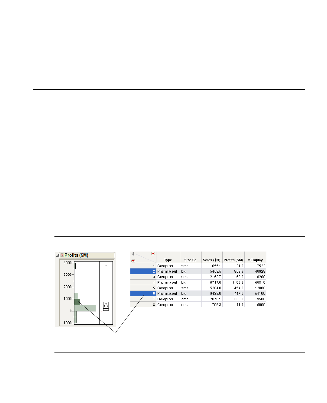
Chapter 1

Clicking on a histogram bar highlights the corresponding data in the associated data table.

Preliminaries

Introducing JMP

Using JMP statistical software, you can interact with your graphs and data to do the following:

Discover Using graphics, you can see patterns and relationships in your data, and find data that does

not fit identifiable patterns.

Interact Using JMP interactive features, you can follow up on clues and try different approaches. The

more approaches you try, the more you likely you are to discover trends in your data.

Understand Using graphics, you can see how the data and the model work together to produce the

statistics. Because JMP is a progressively disclosed system, you learn statistics methods in the right context.

Here are just a few of the things that you can do with JMP:

• Interact with data tables and reports.

• Compute values using the Formula Editor.

• Design experiments.

• Use scripting features to automate frequently used processes.

• Open SAS data sets, run stored processes, and submit SAS code.

Figure 1.1 Interacting with JMP

Contents

Prerequisites . . . . . . . . . . . . . . . . . . . . . . . . . . . . . . . . . . . . . . . . . . . . . . . . . . . . . . . . . . . . . . . . . . . . . . . 3

JMP Terminology . . . . . . . . . . . . . . . . . . . . . . . . . . . . . . . . . . . . . . . . . . . . . . . . . . . . . . . . . . . . . . . . 3

Learning about JMP . . . . . . . . . . . . . . . . . . . . . . . . . . . . . . . . . . . . . . . . . . . . . . . . . . . . . . . . . . . . . . . . . 3

About JMP Documentation . . . . . . . . . . . . . . . . . . . . . . . . . . . . . . . . . . . . . . . . . . . . . . . . . . . . . . . . 3

Use JMP Help . . . . . . . . . . . . . . . . . . . . . . . . . . . . . . . . . . . . . . . . . . . . . . . . . . . . . . . . . . . . . . . . . . . 7

Use Tutorials . . . . . . . . . . . . . . . . . . . . . . . . . . . . . . . . . . . . . . . . . . . . . . . . . . . . . . . . . . . . . . . . . . . . 7

Access Sample Data Tables . . . . . . . . . . . . . . . . . . . . . . . . . . . . . . . . . . . . . . . . . . . . . . . . . . . . . . . . . 7

Learn About Statistical and JSL Terms. . . . . . . . . . . . . . . . . . . . . . . . . . . . . . . . . . . . . . . . . . . . . . . . . 8

Learn JMP Tips and Tricks . . . . . . . . . . . . . . . . . . . . . . . . . . . . . . . . . . . . . . . . . . . . . . . . . . . . . . . . . 8

Access Resources on the Web. . . . . . . . . . . . . . . . . . . . . . . . . . . . . . . . . . . . . . . . . . . . . . . . . . . . . . . . 8

Conventions . . . . . . . . . . . . . . . . . . . . . . . . . . . . . . . . . . . . . . . . . . . . . . . . . . . . . . . . . . . . . . . . . . . . . . . 8

Common Features Throughout Platforms. . . . . . . . . . . . . . . . . . . . . . . . . . . . . . . . . . . . . . . . . . . . . . . . . 9

Launch Window Features . . . . . . . . . . . . . . . . . . . . . . . . . . . . . . . . . . . . . . . . . . . . . . . . . . . . . . . . . . 9

Script Menus. . . . . . . . . . . . . . . . . . . . . . . . . . . . . . . . . . . . . . . . . . . . . . . . . . . . . . . . . . . . . . . . . . . . 11

Automatic Recalc Feature . . . . . . . . . . . . . . . . . . . . . . . . . . . . . . . . . . . . . . . . . . . . . . . . . . . . . . . . . . 13

Chapter 1 Preliminaries 3

Prerequisites

Before you begin using JMP, note the following information:

• You can use many JMP features, such as data manipulation, graphs, and scripting features, without any statistical knowledge.

• A basic understanding of central statistical concepts, such as mean and variation, is recommended.

• Analytical features require statistical knowledge appropriate for the feature.

JMP Terminology

• You can enter, view, edit, and manipulate data using data tables. In a data table, each variable is a column, and each observation is a row.

• You can access a platform from the that you can use to analyze data and work with graphs.

• Platforms use these windows:

– Launch windows where you set up and run your analysis.

– Report windows showing the output of your analysis.

• Report windows normally contain the following items:

– A graph of some type (such as a scatterplot or a chart).

–Specific reports that you can show or hide using the disclosure button .

–Platform options that are located within red triangle menus .

Analyze and Graph menus. Platforms contain interactive windows

Learning about JMP

JMP provides numerous resources to help you learn about the software. Most of them can be found within the

Help menu. You can also access context-sensitive Help from within JMP.

Note: For further information about all of the options in the Help menu, see Using JMP.

About JMP Documentation

You can view the JMP documentation suite by selecting Help > Books.

Table 1.1 describes documents in the JMP documentation suite and the purpose of each document.

4 Preliminaries Chapter 1

Prerequisites

Ta bl e 1 .1 About JMP Documentation

Document Who Should Read This

Document

Discovering JMP If you are not familiar with

JMP, start here.

Using JMP If you want to understand

JMP data tables and how to perform basic operations in JMP, start here.

Basic Analysis and Graphing

If you want to perform basic analysis and graphing functions.

What this Document Covers

Introduces you to JMP and gets you started using JMP

• General JMP concepts and features that span across all of JMP

• Material in these JMP Starter categories: File, Tables, and SAS

• These Analyze platforms:

– Distribution

–Fit Y by X

–Matched Pairs

• Many basic graphing platforms

• Material in these JMP Starter categories: Basic and Graph

Chapter 1 Preliminaries 5

Prerequisites

Ta bl e 1 .1 About JMP Documentation (Continued)

Document Who Should Read This

Document

Modeling and Multivariate Methods

If you want to perform modeling or multivariate methods

What this Document Covers

• These Analyze platforms:

–Fit Model

– Screening

–Nonlinear

–Neural

– Gaussian Process

– Partition

– Time Series

– Categorical

– Choice

– Multivariate

– Cluster

– Principal Components

– Discriminant

– PLS (Partial Least Squares)

–Item Analysis

• These Graph platforms:

–Profilers

–Surface Plot

• Material in these JMP Starter categories: Model, Multivariate, and Surface

6 Preliminaries Chapter 1

Prerequisites

Ta bl e 1 .1 About JMP Documentation (Continued)

Document Who Should Read This

Document

Quality and Reliability Methods

If you want to perform quality control or reliability engineering

Design of Experiments If you want to design

experiments

What this Document Covers

• Life Distribution

• Fit Life by X

•Recurrence Analysis

• Degradation

• Survival

• Fit Parametric Survival

• Fit Proportional Hazards

• These Graph platforms:

– Variability/Gauge Chart

– Control Charts

– Capability

– Pareto Plot

– Diagram (Ishikawa)

• Material in these JMP Starter window categories: Reliability, Measure, and Control

• Everything related to the

DOE menu

• Material in this JMP Starter window category: DOE

Scripting Guide If you want to use the JMP

A reference guide for using JSL commands

Scripting Language (JSL)

In addition, the New Features document is available at http://jmp.com/support/downloads/

documentation.shtml.

Note: The Books menu also contains two reference cards: The JMP Menu Card describes JMP menus, and the JMP Quick Reference Card describes JMP keyboard shortcuts. You can print these for ease of use.

Chapter 1 Preliminaries 7

Prerequisites

Use JMP Help

You can access JMP Help in two ways:

• Access the context-sensitive Help by selecting the Help tool from the tool anywhere in a data table or report window to see the Help for that area.

• Within a window, click on the

Search and view JMP Help using the

Use Tutorials

You can access JMP tutorials by selecting Help > Tutorials. The first item on the Tutorials menu is the

Tutorials Directory. This opens a new window with all the tutorials grouped by category.

If you are not familiar with JMP, then start with the interface and explains the basics of using JMP.

The rest of the tutorials help you with specific aspects of JMP, such as creating a pie chart, using Graph Builder, and so on.

Access Sample Data Tables

All of the examples in the JMP documentation suite use sample data. To access JMP’s sample data tables, select

Help > Sample Data. From here, you can do the following:

• Open the sample data directory.

• Open an alphabetized list of all sample data tables.

• Find a sample data table within a category.

To ol s menu. Place the Help

Help button.

Help > Contents, Search, and Index options.

Beginners Tutorial. It steps you through the JMP

Alternatively, the sample data tables are installed in the following directory:

On Windows:

C:\Program Files\SAS\JMP\9\Support Files <language>\Sample Data

On Macintosh: \Library\Application Support\JMP\9\<language>\Sample Data

8 Preliminaries Chapter 1

Conventions

Learn About Statistical and JSL Terms

The Help menu contains the following indexes:

Ta bl e 1 .2 Descriptions of Help Menu Indexes

Statistics Index

JSL Functions

Object Scripting

Provides definitions of statistical terms.

Provides definitions of JSL functions.

Provides a list of JSL scriptable objects and the messages that can be sent to those objects.

DisplayBox Scripting

Provides a list of the JSL objects that comprise a JMP report.

For more details about these indexes, see Using JMP.

Learn JMP Tips and Tricks

When you first start JMP, you see the Tip of the Day window.

To turn off the Tip of the Day, clear the

Help > Tip of the Day. Or, you can turn it off using the Preferences window. See the Using JMP book.

You can use the JMP Quick Reference Card to learn more advanced commands in JMP. View this document by selecting

Help > Books > JMP Quick Reference Card.

Access Resources on the Web

To access JMP resources on the Web, select Help > JMP.com or Help > JMP User Community.

The

JMP.com option takes you to the JMP Web site, and the JMP User Community option takes you to

JMP online user forums.

Show tips at startup check box. To view it again, select

Conventions

The following conventions help you relate written material to information that you see on your screen.

• Most open data table names that are used in examples appear in

Animals.jmp) in this document. References to variable names in data tables and items in reports also

appear in

Note: Special information, warnings, and limitations are noted as such in boldface.

• Reference to menu names (

• Words or phrases that are important or have definitions specific to JMP are in italics the first time they occur in the text. For example, the word platform is in italics the first time you see it. Most words in italics are defined when they are first used unless clear in the context of use.

Helvetica font (Animals or

Helvetica according to the way they appear on the screen or in the documentation.

File menu) or menu items (Save option) appear in Helvetica bold.

Chapter 1 Preliminaries 9

Common Features Throughout Platforms

The following features are common to multiple areas of JMP:

• “Launch Window Features,” p. 9

• “Script Menus,” p. 11

• “Automatic Recalc Feature,” p. 13

Launch Window Features

Each analysis platform prompts you with a launch window. Table 1.3 describes three panes that all launch windows have in common.

Ta bl e 1 .3 Descriptions of Common Panes in Launch Windows

Select Columns

Cast Selected Columns into Roles

Action

Lists all of the variables in your current data table. For details about the red triangle menu, see “Columns Filter

Menu,” p. 10.

Moves selected columns into roles (such as Y, X, and so on.) You cast a column into the role of a variable (like an actor is cast into a role). See “Cast Selected Columns

into Roles Buttons,” p. 10.

This pane does not exist in the Graph Builder platform.

performs the analysis.

Cancel stops the analysis and quits the launch window.

Remove deletes any selected variables from a role.

Recall populates the launch window with the last

analysis that you performed.

Help takes you to the Help for the launch window.

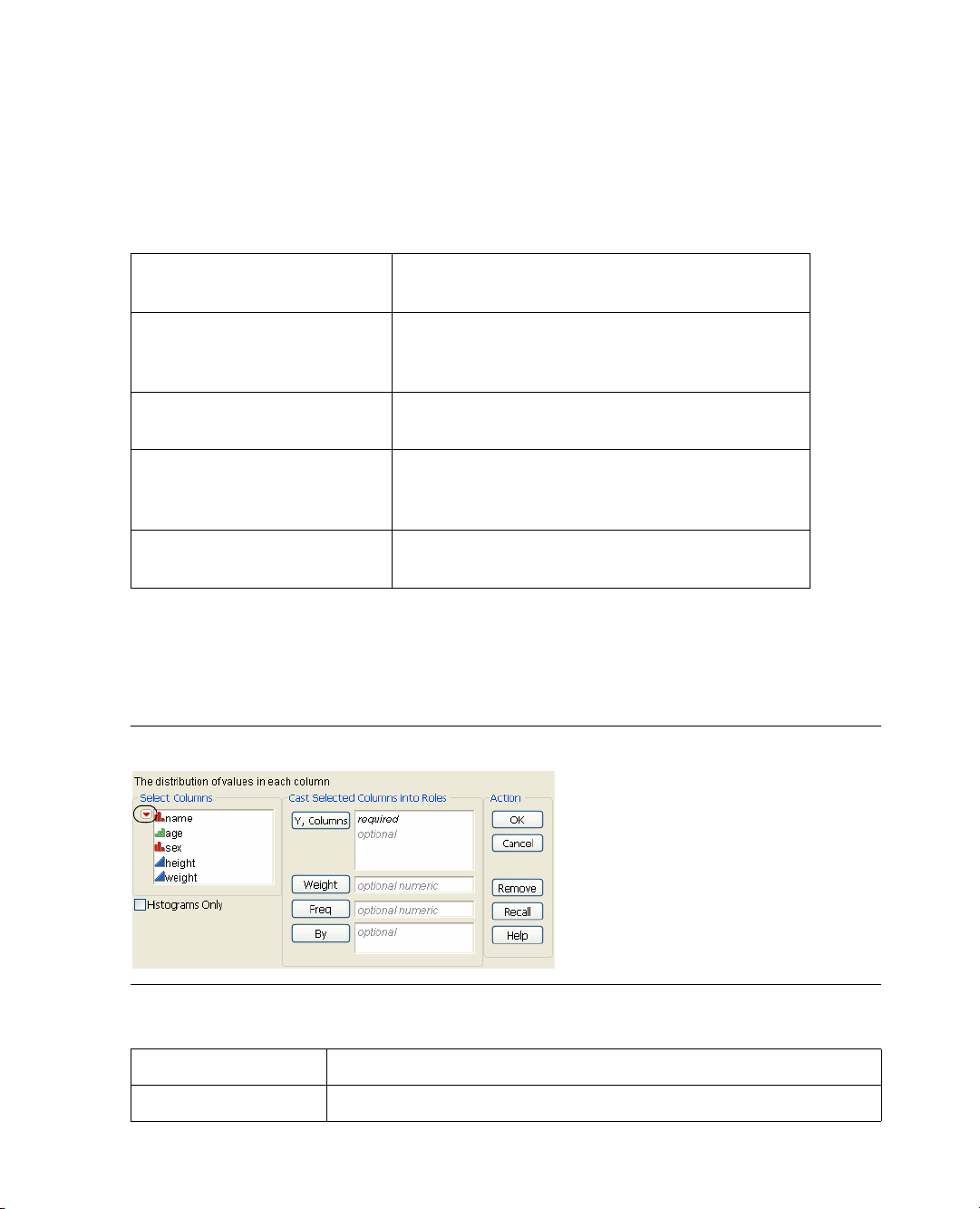
10 Preliminaries Chapter 1

Common Features Throughout Platforms

Cast Selected Columns into Roles Buttons

Table 1.4 describes buttons that appear frequently throughout launch windows. Buttons that are specific to certain platforms are described in the chapter for the platform.

Ta bl e 1 .4 Descriptions of Common Buttons in Launch Windows

Weight

Freq

Columns Filter Menu

In most of the platform launch windows there is a Column Filter menu. This menu appears as a red triangle within the Select Columns panel.

Figure 1.2 Example of the Columns Filter Menu

Identifies a column as a response or dependent variable whose distribution is to be studied.

Identifies a column as an independent, classification, or explanatory variable whose values divide the rows into sample groups.

Identifies the data table column whose variables assign weight (such as importance or influence) to the data.

Identifies the data table column whose values assign a frequency to each row. This option is useful when a frequency is assigned to each row in summarized data.

Identifies a column that creates a report consisting of separate analyses for each level of the variable.

Ta bl e 1 .5 Options within the Columns Filter Menu

Reset

Sort by Name

Resets the columns to its original list.

Sorts the columns in alphabetical order by name.

Chapter 1 Preliminaries 11

Common Features Throughout Platforms

Ta bl e 1 .5 Options within the Columns Filter Menu

Continuous

Ordinal

Nominal

Numeric

Character

Match case

Name Contains

Name Starts With

Name Ends With

Script Menus

The red triangle menu at the top level of every JMP report contains a Script menu.

Shows or hides columns whose modeling type is continuous.

Shows or hides columns whose modeling type is ordinal.

Shows or hides columns whose modeling type is nominal.

Shows or hides columns whose data type is numeric.

Shows or hides columns whose data type is character.

(Only applicable to the Name options below) Makes your search case-sensitive.

Searches for column names containing specified text. To remove the text box, select

Reset.

Searches for column names that begin with specified text. To remove the text box, select

Reset.

Searches for column names that end with specified text. To remove the text box, select

Reset.

Figure 1.3 The Script menu

Most of these options are the same throughout JMP. A few platforms add extra options that are described in the specific platform chapters. Table 1.6 lists the Script menu options that are common to all platforms.

12 Preliminaries Chapter 1

Common Features Throughout Platforms

Ta bl e 1 .6 Descriptions of Script Options

Redo Analysis

Relaunch Analysis

Automatic Recalc

Copy Script

Save Script to Data Table

Save Script to Journal

Save Script to Script Window

Save Script to Report

Save Script for All Objects

If the values in the data table that was used to produce the report have changed, this option duplicates the analysis based on the new data. The new analysis appears in a new report window.

Opens the platform Launch window and recalls the settings used to create the report.

Automatically updates analyses and graphics when data table values change. See “Automatic Recalc Feature,” p. 13.

Places the script that reproduces the report on the clipboard so that it can be pasted elsewhere.

Saves the script to the data table that was used to produce the report.

Saves a button that runs the script in a journal. The script is added to the current journal.

Opens a script editor window and adds the script to it. If you have already saved a script to a script window, additional scripts are added to the bottom of the same script window.

Adds the script to the top of the report window.

If you have By groups or similar multiple reports, a script for each object is saved to the script window. Otherwise, this option is the same as

Save Script to Script Window.

Save Script to Project

Saves the script in a project. If you have a project open that contains the report, the script is added to that project. If you do not have a project that contains the report, a new project is created and the script is added to it.

Data Table Window

Brings the data table that was used to create the report to the front and makes it the active window.

If you have specified a By variable in the platform launch window, the Script All By-Groups menu also appears.

Chapter 1 Preliminaries 13

Common Features Throughout Platforms

Figure 1.4 Example of the Script All By-Groups Menu

If you specified a By variable, the script options in Table 1.7 apply to a report for a single level of a By variable. The

Ta bl e 1 .7 Descriptions of Script All By-Groups Options

Script All By-Groups options apply to the reports for all the levels of the By variable.

Redo Analysis

Relaunch Analysis

Copy Script

Save Script to Data Table

Save Script to Journal

Save Script to Script Window

Automatic Recalc Feature

The Automatic Recalc feature immediately reflects changes that you make to the data table in the corresponding report window. You can make any of the following data table changes:

• exclude or unexclude data table rows

• delete or add data table rows

If the values in the data table that was used to produce the reports have changed, this option duplicates the analysis based on the new data and produces new reports.

Opens the platform Launch window and recalls the settings used to create the reports.

Places the script that reproduces the reports on the clipboard so that it can be pasted elsewhere.

Saves the script to the data table that was used to produce the reports.

Saves a button that runs the script in a journal. The script is added to the current journal.

Opens a script editor window and adds the script to it. If you have already saved a script to a script window, additional scripts are added to the bottom of the same script window.

This powerful feature immediately reflects these changes to the corresponding analyses, statistics, and graphs that are located in a report window.

14 Preliminaries Chapter 1

Common Features Throughout Platforms

To t u rn o n Automatic Recalc for a report window, click on the platform red triangle menu and select

Script > Automatic Recalc. See Figure 1.3. To turn it off, deselect the same option. You can also turn on Automatic Recalc using JSL.

Note the following:

• By default, platforms in the

Chart > Run Chart

•For some platforms, the

Automatic Recalc is turned off for platforms in the Analyze menu and turned on for

Graph menu. The exceptions are the Capability, Variability/Gauge Chart, and Control

platforms.

Automatic Recalc feature is not appropriate, and therefore is not supported.

These platforms include the following: DOE, Profilers, Choice, Partition, Nonlinear, Neural, Neural Net, Partial Least Squares, Fit Model (REML, GLM, Log Variance), Gaussian Process, Item Analysis, Cox Proportional Hazard, and Control Charts (except Run Chart).

Data Tables and Scripts

The first thing you typically do in JMP is open or create a JMP data table:

Chapter 2

Getting Started

• To import an existing file into JMP, either click the select

File > Open. See “Open Existing JMP Files,” p. 25, for details.

• To manually type data into JMP, either click the

File > New > Data Table. This creates an empty JMP data table, and you can start typing in your data.

See “Create New Data Tables,” p. 24, for details.

This chapter tells you more about getting started with the JMP environment, creating new data tables, importing data into new tables, exporting data to other formats, and getting further assistance.

Figure 2.1 JMP Data Table

Open Data Table button in the JMP Starter or

New Data Table button in the JMP Starter or select

Contents

Before You Start. . . . . . . . . . . . . . . . . . . . . . . . . . . . . . . . . . . . . . . . . . . . . . . . . . . . . . . . . . . . . . . . . . . . .17

The Tip of the Day Window. . . . . . . . . . . . . . . . . . . . . . . . . . . . . . . . . . . . . . . . . . . . . . . . . . . . . . . .17

The JMP Home Window (Windows Only) . . . . . . . . . . . . . . . . . . . . . . . . . . . . . . . . . . . . . . . . . . . .17

The JMP Starter Window . . . . . . . . . . . . . . . . . . . . . . . . . . . . . . . . . . . . . . . . . . . . . . . . . . . . . . . . . .21

Display and Arrange Open Windows . . . . . . . . . . . . . . . . . . . . . . . . . . . . . . . . . . . . . . . . . . . . . . . . 22

Create New Data Tables . . . . . . . . . . . . . . . . . . . . . . . . . . . . . . . . . . . . . . . . . . . . . . . . . . . . . . . . . . . . . 24

Open Existing JMP Files . . . . . . . . . . . . . . . . . . . . . . . . . . . . . . . . . . . . . . . . . . . . . . . . . . . . . . . . . . . . . .25

Import Data . . . . . . . . . . . . . . . . . . . . . . . . . . . . . . . . . . . . . . . . . . . . . . . . . . . . . . . . . . . . . . . . . . . . . . 26

Open Text Files . . . . . . . . . . . . . . . . . . . . . . . . . . . . . . . . . . . . . . . . . . . . . . . . . . . . . . . . . . . . . . . . . 27

Open a Text File in a Text Editing Window . . . . . . . . . . . . . . . . . . . . . . . . . . . . . . . . . . . . . . . . . . . .32

Import Text from the Script Window . . . . . . . . . . . . . . . . . . . . . . . . . . . . . . . . . . . . . . . . . . . . . . . . .34

Open Remote Files and Web Pages . . . . . . . . . . . . . . . . . . . . . . . . . . . . . . . . . . . . . . . . . . . . . . . . . . .34

Open SPSS Files . . . . . . . . . . . . . . . . . . . . . . . . . . . . . . . . . . . . . . . . . . . . . . . . . . . . . . . . . . . . . . . . .36

Open Excel Files . . . . . . . . . . . . . . . . . . . . . . . . . . . . . . . . . . . . . . . . . . . . . . . . . . . . . . . . . . . . . . . . .37

Open SAS Data Sets . . . . . . . . . . . . . . . . . . . . . . . . . . . . . . . . . . . . . . . . . . . . . . . . . . . . . . . . . . . . . .38

Create SAS Transport Files in SAS. . . . . . . . . . . . . . . . . . . . . . . . . . . . . . . . . . . . . . . . . . . . . . . . . . . 40

E-mail Tables and Reports (Windows Only) . . . . . . . . . . . . . . . . . . . . . . . . . . . . . . . . . . . . . . . . . . . . . . .41

Encrypt and Decrypt Scripts . . . . . . . . . . . . . . . . . . . . . . . . . . . . . . . . . . . . . . . . . . . . . . . . . . . . . . . . . . .41

Chapter 2 Getting Started 17

Before You Start

Before you begin using JMP, familiarize yourself with its initial windows: the Tip of the Day window, JMP Home Window, and JMP Starter window.

The Tip of the Day Window

When JMP opens, you see the Tip of the Day window. This window provides tips about using JMP that you might not know. Some tips are basic introductory information, and others give hidden power features that you should learn after getting comfortable with the basics.

The Tip of the Day window has the following features:

•

Show tips at startup When checked, displays the Tip of the Day window each time you start JMP.

This option is also accessible in

of the Day at startup

•

Enter Beginner’s Tutorial Click to start the beginner’s tutorial. This tutorial introduces beginners to

JMP and how its commands and controls work. To access the other tutorials, select

•

Previous Tip Returns to the previous tip in the Tip of the Day window.

•

Next Tip Advances to the next tip in the Tip of the Day window.

File (JMP on the Macintosh) > Preferences > General > Show the Tip

Help > Tutorials.

The

Tip of the Day folder is installed with JMP. It contains HTML files and images that are used for

producing the Tip of the Day window.

Note: Add your own tips by naming them tipXX.htm, where XX is the next unused number in a tip

filename.

To open the Tip of the Day window after closing it, select

The JMP Home Window (Windows Only)

When you open JMP on Windows, the JMP Home Window is displayed behind the Tip of the Day window. The JMP Home Window provides access to the following features:

• JMP menus and toolbars. See the “Personalizing JMP” chapter for details.

• Recent Files: Shows a list of files you recently opened. See “Work with Recent Files,” p. 18 for details. (These files are also displayed in the

• Window List: Shows a list of open JMP windows. See “Work with Open Windows,” p. 20 for details. (You select

View > Window List to display the list in a new window.)

File > Recent Files menu.)

Help > Tip of the Day.

18 Getting Started Chapter 2

open recent files

open windows

filter the recent files

clear the recent files filters

preview of the open data table

Before You Start

Figure 2.2 Features of the JMP Home Window

Work with Recent Files

Note: By default, the JMP Home Window appears when you open JMP. You can set the preferences to display the JMP Starter or Window List instead. (Select from the

Window

Initial JMP Window list.) To display the Home Window at any time, select View > Home

. Alternatively, click the JMP Home Window button in the lower right corner of most JMP

File > Preferences > General and select an option

windows. To display the Window List at any time, select View > Window List.

The Recent Files list provides quick access to files that you recently opened in one of the following ways: by selecting

File > Open, clicking the Open toolbar button, or dragging and dropping the file into the Home

Window. You can double-click one or more files to open them, filter the list to display only certain types of files, and clear the list.

When JMP cannot find the file that you recently opened, the filename is grayed out in the list. Right-click the filename and select

Remove From List to clear it from the list.

Chapter 2 Getting Started 19

Before You Start

To O p en R e ce nt F i le s

1. To open one file, do one of the following:

– Double-click the filename.

– Right-click the filename, then select

Open. (This option does not appear for non-JMP files, such as

text files.)

– Select the filename, then select the

Open button on the Recent Files bar.

2. To open several files, select the filenames and do one of the following:

– Press ENTER.

– Right-click, then select

– Select the

Open button on the Recent Files bar.

Open.

3. To open all files, click in the Recent Files window and do one of the following:

– Hold down the CTRL key, press A, and then press ENTER.

– Hold down the CTRL key, press A, right-click, and then select

– Hold down the CTRL key, press A, and then select the

Note: When you double-click a non-JMP file (such as a text file) in the Recent Files list, JMP applies your

import preferences to arrange the data. This also occurs when you click the

Open.

Open button on the Recent Files bar.

Open button on the Recent

Files bar. You can instead select the import method or open the file in a text editing window when you right-click a file in the list. (Your import preference is bolded in the right-click menu.) For details about JMP preferences, see “Text Data Files,” p. 454 in the “JMP Preferences” chapter. For details about importing text files, see “Import Data,” p. 26.

To Filter the Recent Files List and Clear the Filters

1. Click the button on the Recent Files bar.

2. Select the type of files that you want to display. The file types vary depending on which file types you have recently opened. Some common file types are described in the following table.

Ta bl e 2 .1 Descriptions of File and Report Filtering Options

All Files

Data Tables

Excel Files

Other Data Files

Shows all file types in the list.

Shows only data tables in the list.

Shows only Excel files in the list.

Shows data file types other than JMP tables or Excel files (such as .sav files) in the list.

All Data Files

Scripts

Shows all data tables, Excel files, and other data files in the list.

Shows only scripts in the list.

20 Getting Started Chapter 2

Before You Start

3. To show several types of files (for example, data tables and Excel files), repeat the preceding steps and

select a different file type.

4. To remove the filter for a specific file type, click the button on the Recent Files bar, and then deselect that file type.

5. To remove filters so that all files are displayed in the list, click the button on the Recent Files bar. (If this button is grayed out, no filters are selected.) Alternatively, select

All Files from the Filter drop-down

menu.

To Clear the Recent Files List

• To clear one file, right-click the file and select

• To clear the entire list, press CTRL+A, right-click, and then select

• To clear selected files, select those files, right-click, and then select

• To clear one or more files, select them, and then press DELETE.

Work with Open Windows

The Window List displays a list of open JMP windows, such as windows for data tables, scripts, and tutorials. The list also lets you quickly hide and rearrange JMP windows. For example, you can display a data table and its open reports side-by-side or tile some types of JMP windows. The tiled windows are all displayed at once to fill the screen. If you are using JMP on your primary monitor and have an extended desktop, the tiled windows are displayed on the second monitor if necessary.

The Window List is displayed in the JMP Home Window. However, you can open the list at any time by selecting

View > Window List. The list appears in a new window.

Note: To deselect the selected window names, right-click and select Clear Selections.

To D i s p l a y O p en W i nd o w s

• To display one window in the Window List, double-click the window name. Alternatively, right-click the window name and select

• To display several windows in the Window List, select the window names, right-click, then select

Remove from List.

View.

To Rearrange Open Windows

• To display a data table and its reports side-by-side, select the files, right-click them in the Window List, then select

Arrange.

• To display several windows at once, hold down the CTRL key, select the window names, right-click, and select

Arrange.

• To display all windows at once, right-click in the Window List and select and select

Arrange.

• To display windows behind other JMP windows, right-click the window names, then select

Back

Select All. Right-click again

Move To

Chapter 2 Getting Started 21

Before You Start

To Hide and Unhide Open Windows

• To hide windows, right-click the window names, then select

Hide.

The names of the hidden windows are grayed out in the Window List. The hidden windows are also no longer displayed on the Windows task bar.

• To unhide windows, right-click the grayed-out window names, then select

Unhide.

To Filter the Window List and Clear the Filters

1. Click the button on the Window List bar.

2. Select the window type that you want to show.

Only windows of the selected type appear.

3. To show several types of windows (for example, data tables and scripts), repeat the preceding steps and

select a different window type.

4. To remove the filter for a specific window type, click the button on the Window List bar, and then deselect that window type.

5. To remove filters so that all window names are displayed in the list, click the button on the Window List bar. (If this button is grayed out, no filters are selected.) Alternatively, select

Filter drop-down menu.

All Windows from the

To Display the Window List in Maximized Windows

The Window List can be automatically displayed inside maximized data table, script, journal, and report windows. Then the list is always available when you are working in a maximized window. See “Windows

Specific,” p. 456 in the “JMP Preferences” chapter for details.

To Close the Windows

1. Select the windows that you want to close.

2. Right-click and select

If changes in the windows need to be saved, you are prompted to do one of the following: save all changes, save no changes, display each modified file and then decide whether to save the changes, or cancel to close no windows.

The JMP Starter Window

The JMP Starter Window displays most of the commands found in the main menu and toolbars. For example, you can open data tables and create graphs through the JMP Starter, main menu, or toolbars.

You might find the JMP Starter helpful if you are not familiar with JMP or data analysis, because the Starter describes each option and report. See “Overview of the JMP Starter Window,” p. 391, for details.

To open and close the JMP Starter, select

Close.

View (Window on the Macintosh) > JMP Starter.

22 Getting Started Chapter 2

Before You Start

To display the JMP Starter automatically when you open JMP, do one of the following:

• (Windows) Select

• (Macintosh) Select

Figure 2.3 The JMP Starter

File > Preferences, and then select JMP Starter from the Initial JMP Window list.

JMP > Preferences, and then select Initial Starter Window.

Display and Arrange Open Windows

In JMP, you typically have several windows open at once (for example, data tables, reports, and the JMP Home Window). JMP provides several ways to arrange and display these open windows.

• Select options from the Window menu. See “The Window Menu,” p. 435 for details.

• (Windows only) In the Window List, select options from the right-click menu. See “Work with Open

Windows,” p. 20 for details.

• (Windows only) To display the JMP Home Window, click the lower right corner of most windows, or hold down CTRL and press 1.

JMP Home Window button in the

Chapter 2 Getting Started 23

previews of open reports

enlarged preview

Before You Start

• (Windows only) To display all open windows side-by-side, do one of the following:

– Select

Note: If you have extended monitors, windows that do not fit on the primary monitor are displayed on the

Window > Arrange > Select All for Arrange and then select Window > Arrange > Arrange

Selected Windows

Window > Arrange > Select All for Arrange. In one of the windows, click the Arrange

arrow next to the check box ( ) in the bottom right corner, and then select Arrange

Selected Windows

extended monitors.

• (Windows only) To display specific windows side-by-side, do one of the following:

– Select the check box in the bottom right corner of each window that you want to arrange. Then

select

Window > Arrange > Arrange Selected Windows in one of the windows.

– Select the check box in the bottom right corner of each window that you want to arrange. In one of

the selected windows, click the right corner, and then select

– In each window that you want to arrange, select

select

Window > Arrange > Arrange Selected Windows in one of the windows.

• (Windows only) To display the data table for a report, click the

Arrange Menu arrow next to the check box ( ) in the bottom

Arrange Selected Windows.

Window > Arrange > Select for Arrange. Then

View Associated Data button in

the lower right corner of the report.

• (Windows only) To show an associated report when you are viewing a data table, double-click the thumbnail preview of the report in the bottom pane. (Hover the cursor over the thumbnail to enlarge the preview as shown in the following figure.)

Figure 2.4 Thumbnail Previews of Open Reports

24 Getting Started Chapter 2

Create New Data Tables

To analyze data, you must first create a data table.

To create a new data table:

1. Select

2. Move the cursor onto a cell.

3. Click in the cell. The cursor appears as a line in the cell, as shown in Figure 2.5.

Figure 2.5 A New Data Table

4. Enter a value.

File > New > Data Table. This shows an empty data table with no rows and one numeric

column, labeled

Column 1.

There are several ways to fill a table with values:

• Create new rows and columns and type or paste data into the data grid. (See “Adding and Deleting

Rows,” p. 61.)

• Construct a formula to calculate column values. (See “Creating a Formula,” p. 301.)

• Import data from another application. (See “Import Data,” p. 26.)

• Copy values from another application and paste them into the table.

• Use a measuring instrument to read external measures. (See “Reading in Real-Time Data (Windows

Only),” p. 386 in the “External Data and Analytical Sources” chapter for details.)

• Drag columns from one table to another.

See “Entering, Editing, and Managing Data,” p. 43, for details about how to format, edit, and work with data tables.

Chapter 2 Getting Started 25

Open Existing JMP Files

If you want to import a file that is a JMP data table (.jmp), script (.jsl), journal (.jrn), or report (.jrp):

1. Select

File > Open.

2. Select the file type from the window that appears.

3. (Optional, Windows only) Select the

Select this filter the next time this dialog is invoked option to

open the same file type every time. This option is available for any file filter, including text import options. See “Open Text Files,” p. 27.

File Type Operating System Instructions for Opening

JMP data table

Windows From the list next to File name (or the Files of type list on

Windows XP), select

JMP Data Tables.

The highlighted table’s notes and number of rows and columns appear at the bottom of the window. Select the check box beside

Select Columns to display only certain columns in the data

table when opened.

Macintosh The highlighted table’s notes and number of rows and columns

appear at the bottom of the window. Select the check box beside

Select columns before opening to display only certain

columns in the data table when opened.

JMP script Windows 1. From the list next to

Windows XP), select

2. Select a script. The

File name (or the Files of type list on

JMP Files or JMP Scripts.

Run this script only option appears at

the bottom of the window. Check this option to automatically begin running the script.

Macintosh After selecting a script, the

the bottom of the window. Check it to automatically begin running the script.

JMP journal, report, or project

Windows From the list next to

Windows XP), select

Projects

Macintosh No further action is necessary.

3. Select the name of the file that you would like to open.

4. Click

Open.

Note: JMP can open JMP files that are version 3 and later.

Run after opening option appears at

File name (or the Files of type list on

JMP Journals, JMP Reports, or JMP

26 Getting Started Chapter 2

Import Data

You can import many file formats into JMP and save them as data tables. JMP opens many files by default. Other files, such as Microsoft Excel 2007 files, require specific Open Database Connectivity (ODBC) drivers.

Supported by default:

• Comma-separated (

•

.dat files that consist of text

•ESRI shapefiles (

• Flow Cytometry versions 2.0 and 3.0 (

•HTML (

.htm, .html)

• Microsoft Excel 1997–2003 (

• Minitab (

• Plain text (

.mtw, .mtp, but not .mpj)

.txt)

• SAS transport (

• SAS versions 6–9 on Macintosh (

• SAS versions 6–9 on Windows (

.csv)

.shp)

.fcs)

.xls)

.xpt, .stx)

.sas7bdat, .ssd, .ssd01, .saseb$data)

.sd2, .sd5, .sd7, .sas7bdat)

• SPSS files (.sav)

• Tab-separated (

.tsv)

Note: “Open SAS Data Sets,” p. 38 in this chapter explains how to open SAS version 6 data sets without a SAS server. To open SAS 7–9 data sets, you must connect through a SAS server. See “Opening SAS Data

Sets through a SAS Server,” p. 362 in the “External Data and Analytical Sources” chapter for details.

Require ODBC drivers:

• Database (dBASE) (

• Microsoft Access Database (

• Microsoft Excel 2007 (

.dbf, .ndx, .mdx) is supported with a V3+ compliant ODBC driver.

.mdb) is supported with a V3+ compliant ODBC driver.

.xlsm, .xlsx, .xlsb) is supported with at least a version 3 compliant ODBC driver

installed on the machine. 64-bit JMP requires a 64-bit ODBC driver.

See “Connecting to Databases,” p. 377 in the “External Data and Analytical Sources” chapter for details for working with databases.

Your computer’s available memory affects data import. Very large files might load slowly or not at all. Consider splitting up large files before importing them. In JMP, you can then join or concatenate the tables. For more information, see “Concatenating Data Tables,” p. 252 in the “Reshaping Data” chapter and

“Joining Data Tables,” p. 254 in the “Reshaping Data” chapter.

Note: You can open R code (.R) and SAS program files (.sas) in JMP, but the text opens in a Script window, not in a data table.

Chapter 2 Getting Started 27

Import Data

Open Text Files

You can open text files with the extensions .txt, .csv, and .tsv, and the text is converted to a data table. Files with the character, or they can be fixed-width files.

In the JMP preferences, you change the import settings so that JMP determines the best way to structure and format the data table. Alternatively, you can manually select the import settings as you open the file. Another option is opening the file in the Script editor, editing the content, and then importing the content. This option is helpful when you need to add text delimiters or modify the text.

Table 2.2 lists the steps involved in opening text files directly.

Ta bl e 2 .2 Opening Text Files

.dat extension that consist of text are also supported. Text files can be delimited using almost any

Windows

Automatically Determining Data Arrangement

1. Select File > Open.

2. From the list next to

Files of type list on Windows XP),

select

Text Files.

File name (or the

3. To use the import rules from the preferences, select

Import preferences

Data, using Text

. (See “Text Data

Files,” p. 454 in the “JMP Preferences”

chapter.)

To have text import use its best guess to arrange the data, select the

best guess

(Optional) Select

next time this dialog is invoked

option.

Select this filter the

Data, using

to apply the filter that you chose by default.

4. Select the file that you want to open.

5. Click

Open.

Tip: The JMP Home window provides a

shortcut to the above steps if you recently opened the file. Right-click the file in the Recent Files list and select

(Preferences)

or Import (Best Guess).

Import

(Your import preference is bolded in the right-click menu.)

Manually Specifying Data Arrangement

1. Select

2. From the list next to

3. Select

File > Open.

File name (or the

Files of type list on Windows XP),

select

Text Fi l e s .

Data with Preview next to

Open at the bottom of the window.

4. Select the file that you want to open.

5. Click

Open.

6. Complete the Text Import window. See “Text Import Preview Options,”

p. 28, for details.

7. Click

Import.

Tip: The JMP Home window provides a

shortcut to the above steps if you recently opened the file. Right-click the file in the Recent Files list and select

(Preview)

Import

28 Getting Started Chapter 2

Import Data

Ta bl e 2 .2 Opening Text Files (Continued)

Automatically Determining Data Arrangement

Macintosh

1. Select File > Open.

2. Select the file that you want to open.

3. From the

(Best Guess) Preferences)

4. Click

Note: On Windows, JMP can open text files in your computer’s default text editor. Select File > Open, and

then select

All Files (*.*) from the File name list (or the Files of type list on Windows XP). Select the text

file, and then select Use default program to open. Uncheck to open as text.

For details about importing text from a Script window, see “Import Text from the Script Window,” p. 34.

Text Import Preview Options

When you open a text file that JMP supports, JMP can show a preview of the text before saving the file as a data table. This option lets you manually arrange and format the data. For example, you can specify the end-of-line character or strip quotation marks.

Open As field, select Data

or Data (Using

Open.

Manually Specifying Data Arrangement

1. Select

File > Open.

2. Select the file that you want to open. From the

(Using Preview)

3. Click

Open As field, select Data

Open.

4. Complete the Text Import Preview window. See “Text Import Preview

Options,” p. 28, for details.

5. Click

Import.

JMP detects the file’s structure and shows options for importing text with either delimiters or fixed width fields. If JMP chooses the wrong file structure, click the

Delimited fields or Fixed width fields radio button

to import the data as the correct format. (For example, the fixed width window might appear when your file is actually delimited.)

Chapter 2 Getting Started 29

Import Data

The text import preview options are shown in the following figures:

Figure 2.6 Text Import Preview for Fixed Width Files

Figure 2.7 Text Import Preview for Delimited Files

30 Getting Started Chapter 2

Import Data

Charset

Select the character set used in the imported file, or let JMP detect the character set. If incorrect characters are displayed in the imported file, open the file again and select another character set.

End of Field (Available only in the Delimited Import window) Select the check boxes beside the

character that marks the end of a field. Alternatively, select the check box beside

Other and enter a

character if the appropriate character is not listed.

End of Line (Available only in the Delimited Import window) Select the check boxes beside the

character that marks the end of a line (row). Alternatively, select the check box beside

Other and

enter a character if the appropriate character is not listed. Note that when JMP finds double quotation marks, the delimiter rules change to look for an end double quotation mark. Other text delimiters, including spaces embedded within the quotes, are ignored and treated as part of the text string.

File contains column names on line Tell JMP where to find data to use as column names. For

example, if the column names in your text file are on line (row) 3, select this option and type 3 in the check box. Otherwise, JMP uses the data in the first line of the imported file as the column name in the JMP data table or takes the first line as data.

Data starts on line Specify the number of the first line that contains data.

Number of Lines Specify the number of lines (rows) that the imported file contains.

Strip enclosing quotation marks Available only on fixed-width imports. Select this check box when

you want JMP to remove quotation marks that enclose data in the text file.

Two-digit year rule Specify how year numbers are displayed.

•

10-90 (default) Refer to Table 2.3 to see how the 10-90 rule works in JMP.

•

19xx JMP adds 19 before dates in the file that have only two digits that indicate the year.

•

20xx JMP adds 20 before dates in the file that have only two digits that indicate the year.

•

Custom Lets you open and implement a JSL script that customizes how JMP handles dates.

Recognize apostrophe as quotation mark (not recommended) (Available only in the Delimited

Import window). Use this option only if your data comes from a nonstandard source that places apostrophes around data fields rather than quotation marks.

Ta bl e 2 .3 The 10-90 Rule for Importing Two-Digit Years

Last Two Digits of Current Year (as Shown on Your Computer)

Two-Digit Date in Text File JMP Display Format

Between 11 and 89 not applicable The current century is used as the

first two digits.

Between 00 and 10 Less than 90 The current century is used as the

first two digits.

Between 90 and 99 The previous century is used as the

first two digits.

Chapter 2 Getting Started 31

character column

numeric column excluded column numeric column

format

Import Data

Ta bl e 2 .3 The 10-90 Rule for Importing Two-Digit Years (Continued)

Last Two Digits of Current Year (as Shown on Your Computer)

Two-Digit Date in Text File JMP Display Format

Between 90 and 00 Between 0 and 10 The next century is used as the first

two digits.

Between 11 and 99 The current century is used as the

first two digits.

When you are finished selecting the settings, click Next. The next window shows each column’s modeling type. To change the default modeling types, do one of the following:

• Click on the modeling icon to change the modeling type from numeric ( ) to character ( ). Clicking the icon cycles between the modeling type and exclude ( ). Exclude means that the column is not imported.

• To change a numeric column’s data format, select the format from the red triangle menu.

• Click on the column heading to modify the text.

The top of the Text Import window shows a preview of the text file as it appears when imported into a JMP data file. Click the

Figure 2.8 Text Import Preview Window with Column Options

Import button to import the data.

6. When you are finished, click Import to complete the text import.

32 Getting Started Chapter 2

Import Data

Open a Text File in a Text Editing Window

You can open a text file in a Script window, where you edit the text. Then you can import the text as a data table. This feature is helpful when you want to reformat the text before importing it as a data table. For example, you might need to insert the correct delimiters or modify the text.

Another option is opening a JMP add-in definition (

.def) file as text and then editing it in a Script window.

To open a text file in a text editing window (Windows):

Files that you recently opened are listed in the JMP Home window. For most files, right-click the text file and select

Open as Plain Text to open the file in a text editing window. JMP add-in definition files cannot

be opened as plain text from the JMP Home window.

When you are opening the file for the first time, follow these steps:

1. Select

File > Open.

2. Do one of the following:

– To open a JMP add-in definition file as text, select

next to

File name (or the Files of type list on Windows XP). Click the Open button arrow, and

then select

– To open other text files, select

Open as Plain Text. The file opens in a Script window. Skip the remaining steps.

Text Files from the list next to File name (or the Files of type list on

All JMP Files or JMP Add-In Files from the list

Windows XP).

Figure 2.9 Select Text Files

Chapter 2 Getting Started 33

Import Data

3. (Optional) To set the default option file type to Text Files, select the check box beside Select this filter

the next time this dialog is invoked

4. Select the file.

5. Select

6. Click

Plain text into Script window next to Open as.

Open.

The text appears in a Script window.

To open a text file in a text editing window (Macintosh):

1. Select

Figure 2.10 Opening a Text Document on the Macintosh

File > Open.

2. Select the file.

3. Select

4. Click

Te xt from the Open As list.

Open.

The text appears in a Script window.

For details about converting the text to a data table, follow step 3 in “Import Text from the Script Window,”

p. 34.

34 Getting Started Chapter 2

Import Data

Import Text from the Script Window

You can import text from the Script window as a data table. The text can be in a table format (for example, from a Microsoft Word document or web page) or in plain text format. This feature is helpful when you want to reformat the text before importing it as a data table. For example, you might need to insert the correct delimiters or modify the text.

JMP uses the import settings in the preferences to determine how to structure and format the text. Some options include removing quotation marks around text and specifying the rows that contain column headings and data. See “Text Data Files,” p. 454 in the “JMP Preferences” chapter for details.

Note: You can also import an entire web page as a data table. See “Open Remote Files and Web Pages,” p. 34

for details.

This section describes how to import text that you paste into the Script window. For details about opening a text file in the Script window, see “Open a Text File in a Text Editing Window,” p. 32.

To import text from the Script window, proceed as follow:

1. Open a new Script window in JMP by selecting

Script

(Macintosh).

2. Copy and paste the text into the Script window.

3. Do one of the following:

– To import all text from the Script window, select

Import as Data

(Macintosh).

– To import specific text, select the text, and then select

Import as Data

(Macintosh).

The text is imported into a JMP data table.

Open Remote Files and Web Pages

You import data from Internet sites, intranet sites, FTP sites, or other computers by selecting File > Internet

Open

. The file paths begin with the Uniform Resource Locators (URLs) http, ftp, or file; a drive letter; or

the path to a network drive (relative or absolute).

You also use this feature to import a Web page on a local or network drive as a data table. When you open a Web page by selecting

SAS stored process reports open in an HTML view. From that view, you can import the file as a data table.

JMP inserts the location of the original data as a note in the data table. For example, the path Z:\example.html is included as a note when you import

File > Open instead, the page opens in a browser, not as a data table.

File > New > Script (Windows) or File > New > New

File > Import as Data (Windows) or Edit >

example.html from the Z drive.

Open a Remote File

1. Select

File > Internet Open. The window shown in Figure 2.11 appears.

Chapter 2 Getting Started 35

Import Data

Figure 2.11 Internet Open Window

2. Enter the URL.

3. Click the list under

Open As, and select the option that specifies how you would like JMP to display the

imported data:

Data Imports the file as a data table.

Web page Opens the Web page in a browser. (Select this option to import data generated by web

page scripts and server-side requests.)

Te xt Opens the file in a JMP Script window. In an HTML file, the HTML tags of a .html file are

displayed.

4. Click

OK.

One of the following occurs:

– The file opens as you specified.

– If you imported a web page as data, a window appears that lists all tables on the page. Select the table

or tables that you want to open, and then click

– If you imported a web page as a web page, select

Select the table or tables that you want to open, and then click

OK. Each table opens in a new data table.

File > Import Data as Data Table in the browser.

OK. Each table opens in a new data

table.

– If the file is on an FTP server, the window in Figure 2.12 appears.

Figure 2.12 FTP Login Window

For an anonymous account, click OK. For an authenticated login, enter your user ID and password. The file then opens as you specified.

Note: Some anonymous FTP servers require a user ID. If the data table does not open, try typing either ftp or anonymous in the User ID text box. Leave the Password text box empty and click OK.

36 Getting Started Chapter 2

Import Data

Open a SAS Stored Process Report as a Data Table

SAS stored processes open reports in an HTML view by default. To open a report as a data table, follow these steps:

1. In the HTML view, select

A window appears that lists the tables found in the Web page.

2. Select the table or tables that you want to import.

3. Click

OK.

Each table is opened as a new data table.

See “Running Stored Processes,” p. 369 in the “External Data and Analytical Sources” chapterfor more information about stored process reports.

Open SPSS Files

JMP opens SPSS files as data tables and maintains several SPSS features:

• General numeric and character data with minimal formatting are supported.

• SPSS date, datetime, and time formats are supported.

• By default, labels are converted to column headings. When you select this option, and the data contains

no labels, the columns are named Column 1, Column 2, and so on.

You also have the option of selecting the conversion method for column headings when opening an SPSS file. The method that you select then overrides the preferences.

To change the default conversion method, select Macintosh). On the General page, deselect Variable names are then imported automatically as column headings.

• The value labels that you defined in the SPSS file are saved as Value Labels column properties. The value

label then appears in each data table cell instead of the original value. For details about Value Label properties, see “Using Value Labels,” p. 151 in the “Properties and Characteristics of Data” chapter.

• Labels and variable names are saved as the column properties SPSS Label and SPSS Name.

File > Import Table as Data Table.

File > Preferences (or JMP > Preferences on

Use SPSS labels for column names during import.

SPSS can assign certain values in a variable to be treated as missing for analyses. For example, the value 64 could be regarded as missing for a ignore values of 64. When you import SPSS into JMP, these values are included in the

Codes

column property for the appropriate variable.

Height variable. Then, the calculation of the distribution of height would

Missing Value

At the time of publication, custom currency formats selected in an SPSS file are not maintained on import. In addition, JMP does not read SPSS data that contains double-byte characters, such as non-Unicode Japanese characters.

Note: As with importing other files, you might experience a delay when opening and saving large SPSS files.

Chapter 2 Getting Started 37

Import Data

Open an SPSS File (Windows)

1. Select

2. From the list next to

(*.sav)

File > Open.

File name (or the Files of type list on Windows XP), select SPSS Data Files

3. Select the SPSS file.

4. (Optional) To specify the column headings, select one of the following options:

–

SPSS Labels creates column headings from SPSS labels.

–

SPSS Variable Names creates column headings from variable names.

5. Click

Open.

JMP opens the file as a data table.

Open an SPSS File (Macintosh)

1. Select

File > Open.

2. Select the SPSS file.

3. (Optional) To specify the column headings, do one of the following

– Deselect

– Select

4. Click

Use SPSS Labels as Headings to convert variable names to column headings.

Use SPSS Labels as Headings to convert labels to column headings.

Open.

JMP opens the file as a data table.

Set JMP column names from

Open Excel Files

When you open an Excel file in JMP, the file is automatically converted to a data table. JMP can automatically convert the first row into column headings. If you do not select this option, the columns are named Column 1, Column 2, and so on.

JMP can also automatically open each worksheet in the spreadsheet as a separate data table. You select this option in the preferences or when you open a spreadsheet. See “General,” p. 443 in the “JMP Preferences” chapter for details about Excel preferences.

JMP also opens Excel files from web sites that do not require you to log in. On Windows, follow the procedure in this section. On Macintosh, use the

and Web Pages,” p. 34 for more information.

Note: In addition to supporting Microsoft Excel 97-2003 files, you can open Excel 2007 files if at least a

version 3 compliant ODBC driver is installed on the machine. In 64-bit JMP, a 64-bit ODBC driver is required.

File > Internet Open command. See “Open Remote Files

38 Getting Started Chapter 2

Import Data

To open an Excel File (Windows):

1. Select

2. From the list next to

File > Open.

File name (or the Files of type list on Windows XP), select Excel 97-2003 Files

(*.xls)

or Excel 2007 (*.xlsm, *.xlsx, *.xlsb).

3. Select the file or enter the URL.

4. (Optional) To convert text in the first row to column headings, select

Excel Row 1 as labels

. If you do not want to import specific worksheets, click Open.

Always next to Always enforce

5. (Optional) To open specific worksheets, do one of the following:

– (Windows 7 and Vista) Click the

one ore more worksheets, and then click

Open button arrow, select Open Selected Worksheets, select

OK. You can also click Select All if you change your mind

and want to import all worksheets.

–(Windows XP) Click

then click

OK.

Allow individual worksheet selection, click Open, select the worksheets, and

The spreadsheet is opened as you indicated.

If you tried to open an Excel 2007 file and do not have the correct ODBC driver installed, an error appears.

To open an Excel file (Macintosh):

1. Select

File > Open.

2. Select the file. (If the filename is grayed out, the required ODBC driver is not installed, so the file type is not supported.)

3. (Optional) To convert text in the first row to column headings, select

4. (Optional) To open specific worksheets, select

5. Click

Open.

Select Individual Excel Worksheets.

Use Excel Labels as Headings.

If you chose to open specific worksheets, select those worksheets from the list, and then click OK. You can also click

Select All if you change your mind and want to import all worksheets.

The spreadsheet is opened as you indicated.

Open SAS Data Sets

SAS data sets are saved in one of many SAS formats:

• Windows formats are

• Macintosh formats are

When you open a data set in JMP, the file opens as a data table. Columns names are assigned as follows:

• On Windows, JMP uses SAS labels as JMP data table column names by default. You can override the default and request that JMP uses SAS variable names as JMP column names. See step 4 below.

• On the Macintosh, JMP uses SAS variable names as table column names by default. After the data is imported as a JMP data table, you can view the SAS labels by double-clicking the column name.

.sd2, .sd5, .sd7, .sas7bdat.

.sas7bdat, .ssd, .ssd01, .saseb$data.

Chapter 2 Getting Started 39

Import Data

The SAS label appears as a Notes property. You can also replace the table column names with the SAS labels by running the script JMP automatically created when it opened the data table. The script is located in the tables panel under the data table name.

Note: This section describes how to open SAS version 6 data sets directly without connecting to a SAS

server first. Later data set versions require SAS server integration. See “Opening SAS Data Sets through a

SAS Server,” p. 362 in the “External Data and Analytical Sources” chapter for details.

To open a SAS data set:

1. Select

2. On Windows, select

File > Open.

SAS Data Sets or Data Files from the list next to File name (or the Files of type

list on Windows XP), as shown in Figure 2.13.

Note: SAS variable names and formats are preserved and can be saved after changes are made to the SAS

data set. See “Save as a SAS Data Set (Windows Only),” p. 108 in the “Saving Tables, Reports, and Sessions” chapter.

3. Select the file.

Figure 2.13 Open SAS Data Set

4. (Optional on Windows) Select any of the following options:

–

Select this filter the next time this dialog is invoked Sets the default file type choice to the

option that you select next to the selected, the default file type will be

File name list (or in the Files of Type list on Windows XP). If

SAS Data Sets the next time you reach this window.

40 Getting Started Chapter 2

Import Data

– SAS variable labels (Windows Vista and Windows 7 only) Uses the SAS variable labels (instead

of variable names) as the column names in the JMP data table.

–

SAS variable names (or Use SAS Variable Names for Column Names on Windows XP) Uses

the SAS variable names (instead of the labels) as the column names in the JMP data table.

–

Data set is password-protected (or Dataset is Password Protected on Windows XP) Select

this check box if you know the file is password protected. See “Opening Password-Protected Data

Sets,” p. 369 in the “External Data and Analytical Sources” chapter for details.

(Optional) Select any of the following for a SAS Transport (.xpt) file:

–

Select member Lets you enter the name of a specific member, or table, for JMP to open.

–

Open all members Opens all members, or tables, in the transport file.

–

Save all members Saves the file as a JMP file as soon as you open it. The file is saved to the same

directory where the SAS transport file was opened.

–

Select Columns Tells JMP to open only certain columns from the transport file. When you click Open, JMP provides a list of columns with checks next to the columns that it intends to open. Add

or remove checks to modify the list.

5. Click

Open.

Note: If you are importing date variables from a SAS file, JMP looks for a SAS date format and translates it

to a JMP date column.

Create SAS Transport Files in SAS

JMP can open SAS transport files that were saved using the SAS XPORT engine. For example, below is sample SAS code that creates a transport file called

data test; input name $ age weight; cards; Susan 12 72 Melanie 10 68 Jonathan 11 77 Sheila 13 67 ; libname misc xport 'C:/test.xpt'; proc copy in=work out=misc; run;

test. (Note: misc and work are SAS libref names.)

Chapter 2 Getting Started 41

E-mail Tables and Reports (Windows Only)

If you are using a Windows operating system, JMP gives you a one-click method of e-mailing a data table and report.

To send e-mail from JMP:

1. Open a data table or create a report.

2. Select

File > Send. The open window is submitted to your default e-mail application. The file is

attached to the e-mail.

Encrypt and Decrypt Scripts

If you want to protect a JMP Scripting Language (JSL) file, you can encrypt it so only someone who knows the password can view it; you can also require a password to run it. This is useful in situations when you want to implement controlled sharing of a script.

To e n cr y pt a sc r i pt :

1. Open the script that you want to encrypt.

2. Select

3. Assign password(s) to encrypt the files:

Edit > Encrypt Script.

– To encrypt a script so that a user can run it without a password, but needs a password to view it,

enter only a decrypt password.

– To encrypt a script so that a user must enter one password to run it and another password to view it,

enter both a run and a decrypt password.

Note: The password must consist of single-byte characters; using a text Input Method Editor (IME) does not work.

4. Click

5. If you entered only a decrypt password, click Yes to confirm that you do not want to assign a run

Figure 2.14 Example of Encrypted Script

6. Save the encrypted script.

OK.

password.

The encrypted script opens in a new window.

42 Getting Started Chapter 2

Encrypt and Decrypt Scripts

To d e cr y pt a JS L s cr i pt :

1. Open the encrypted script in JMP.

2. Select

3. Enter the decrypt password and click

Edit > Decrypt Script.

OK.

The decrypted script opens in a new window.

To r u n a n e n cr y pt ed J SL s cr i p t:

Note: You should examine a script from an unknown source before running it. To examine an encrypted

script, you need the decrypt password.

1. Open the encrypted script in JMP.

2. Select

3. Enter the run password and click

Edit > Run Script.

OK.

The script runs.

If the script references a data table, you are prompted to open the data table, and then the script runs.

If the script requires an empty data table, you must create the table and then run the encrypted script.

Note that entering the run password runs the script, but does not show the script: you must supply the decrypt password to actually view the script.

Chapter 3

Entering, Editing, and Managing Data

Preparing for Analyses

After you import data into JMP or create a new data table, you need to format your data and the table so it will be ready for analysis.

This chapter contains information that helps you:

• Understand parts of a JMP data table

• Specify data types and modeling types

• Select your data’s format

• Edit data tables

• Lock data tables

• Select rows and columns

Contents

Elements of JMP Data Tables . . . . . . . . . . . . . . . . . . . . . . . . . . . . . . . . . . . . . . . . . . . . . . . . . . . . . . . . . .45

Specifying Data Types and Modeling Types. . . . . . . . . . . . . . . . . . . . . . . . . . . . . . . . . . . . . . . . . . . . . . . .55

Entering Data . . . . . . . . . . . . . . . . . . . . . . . . . . . . . . . . . . . . . . . . . . . . . . . . . . . . . . . . . . . . . . . . . . . . . .61

Adding and Deleting Rows . . . . . . . . . . . . . . . . . . . . . . . . . . . . . . . . . . . . . . . . . . . . . . . . . . . . . . . . .61

Adding and Deleting Columns . . . . . . . . . . . . . . . . . . . . . . . . . . . . . . . . . . . . . . . . . . . . . . . . . . . . . 62

Setting Up Initial Data Values . . . . . . . . . . . . . . . . . . . . . . . . . . . . . . . . . . . . . . . . . . . . . . . . . . . . . . .63

Filling Columns with Sequential Data. . . . . . . . . . . . . . . . . . . . . . . . . . . . . . . . . . . . . . . . . . . . . . . . 64

Entering Cell Formulas . . . . . . . . . . . . . . . . . . . . . . . . . . . . . . . . . . . . . . . . . . . . . . . . . . . . . . . . . . . .65

Editing Data and Tables . . . . . . . . . . . . . . . . . . . . . . . . . . . . . . . . . . . . . . . . . . . . . . . . . . . . . . . . . . . . . 66

Editing Cells . . . . . . . . . . . . . . . . . . . . . . . . . . . . . . . . . . . . . . . . . . . . . . . . . . . . . . . . . . . . . . . . . . . 66

Editing Column Names. . . . . . . . . . . . . . . . . . . . . . . . . . . . . . . . . . . . . . . . . . . . . . . . . . . . . . . . . . . 66

Recoding Data. . . . . . . . . . . . . . . . . . . . . . . . . . . . . . . . . . . . . . . . . . . . . . . . . . . . . . . . . . . . . . . . . . 67

Viewing Patterns of Missing Data . . . . . . . . . . . . . . . . . . . . . . . . . . . . . . . . . . . . . . . . . . . . . . . . . . . 68

Finding and Replacing Cell Values . . . . . . . . . . . . . . . . . . . . . . . . . . . . . . . . . . . . . . . . . . . . . . . . . . 69

Reordering Columns . . . . . . . . . . . . . . . . . . . . . . . . . . . . . . . . . . . . . . . . . . . . . . . . . . . . . . . . . . . . . 72

Rows and Columns Context Menus . . . . . . . . . . . . . . . . . . . . . . . . . . . . . . . . . . . . . . . . . . . . . . . . . .73

Copying, Cutting, and Pasting . . . . . . . . . . . . . . . . . . . . . . . . . . . . . . . . . . . . . . . . . . . . . . . . . . . . . .73

Using the Row Editor . . . . . . . . . . . . . . . . . . . . . . . . . . . . . . . . . . . . . . . . . . . . . . . . . . . . . . . . . . . . 76

Changing Table Names . . . . . . . . . . . . . . . . . . . . . . . . . . . . . . . . . . . . . . . . . . . . . . . . . . . . . . . . . . . 77

Locking Tables . . . . . . . . . . . . . . . . . . . . . . . . . . . . . . . . . . . . . . . . . . . . . . . . . . . . . . . . . . . . . . . . . 78

Adding Table Variables . . . . . . . . . . . . . . . . . . . . . . . . . . . . . . . . . . . . . . . . . . . . . . . . . . . . . . . . . . . 79

Creating Scripts. . . . . . . . . . . . . . . . . . . . . . . . . . . . . . . . . . . . . . . . . . . . . . . . . . . . . . . . . . . . . . . . . .82

Selecting Rows and Columns . . . . . . . . . . . . . . . . . . . . . . . . . . . . . . . . . . . . . . . . . . . . . . . . . . . . . . . . . 86

Selecting Excluded, Hidden, or Labeled Rows. . . . . . . . . . . . . . . . . . . . . . . . . . . . . . . . . . . . . . . . . . .88

Selecting Cells with Specific Values . . . . . . . . . . . . . . . . . . . . . . . . . . . . . . . . . . . . . . . . . . . . . . . . . . .88

Selecting a Particular Row or Column. . . . . . . . . . . . . . . . . . . . . . . . . . . . . . . . . . . . . . . . . . . . . . . . .91

Randomly Selecting Rows . . . . . . . . . . . . . . . . . . . . . . . . . . . . . . . . . . . . . . . . . . . . . . . . . . . . . . . . . .91

Inversely Selecting and Selecting All Rows. . . . . . . . . . . . . . . . . . . . . . . . . . . . . . . . . . . . . . . . . . . . . .91

Locating Next and Previously Selected Rows . . . . . . . . . . . . . . . . . . . . . . . . . . . . . . . . . . . . . . . . . . . 92

Using the Keyboard to Select Rows and Columns . . . . . . . . . . . . . . . . . . . . . . . . . . . . . . . . . . . . . . . .93

The Data Filter . . . . . . . . . . . . . . . . . . . . . . . . . . . . . . . . . . . . . . . . . . . . . . . . . . . . . . . . . . . . . . . . . . . . .93

Chapter 3 Entering, Editing, and Managing Data 45

data table panels

data grid

Elements of JMP Data Tables

JMP data are organized into rows and columns referred to as the data table. A data table has two parts, as shown in Figure 3.1: the data table panels at left and the data grid at right.

Figure 3.1 Parts of a Data Table

The data table has the following characteristics:

• Column names can contain any keyboard character, including spaces, and can be up to 255 characters long.

• The maximum length of the data table’s name depends on your computer’s operating system.

• Change the default size and font for names and values selecting Macintosh, select

JMP > Preferences > Fonts.)

File > Preferences > Fonts. (On the

• Column names automatically wrap in the column name area to accommodate the column width that you specify.

• Move column boundaries and enlarge the column to view long values. Adjust widths of all selected columns at once by pressing the ALT key as you drag the double arrow cursor on any of the selected column boundaries.

46 Entering, Editing, and Managing Data Chapter 3

hides or shows the data table panels

Click and drag to adjust the height and width of the panels.

table options

dolumn options

row options

script options

hides or shows the data grid

Elements of JMP Data Tables

• There is no limit to the number of rows or columns in a data table. However, the table must fit in your computer’s memory.

The Data Table Panels

There are three data table panels—the table panel, the columns panel, and the rows panel. The data table panels are arranged to the left of the data grid, as shown in Figure 3.2. These panels contain information about the table and its contents. Each have interactive components, as shown in Figure 3.2.

Figure 3.2 Interacting with the Data Table Panels

The Table Panel

The table panel contains the following elements:

• Data table name

• Red triangle menus containing table and script options

• Table variables

• Table scripts

data table name table variable

table scripts

table options

script options

Chapter 3 Entering, Editing, and Managing Data 47

Elements of JMP Data Tables

Figure 3.3 Example of a Table Panel

Table Options

Clicking on the red triangle icon next to the data table name gives you these options:

Ta bl e s Gives you the same options as selecting the Tab le s command from the main menu, which is

discussed in detail in “Reshaping Data,” p. 227.

New Table Variable Lets you create a new table variable, which can be text or any other constant

character value that you always want to be available in the data table. Table variables are mostly used to document tables. You can also access them when you are using the formula editor so they can be incorporated into formulas or JSL scripts. JMP sometimes automatically creates table variables, such as:

• If you open a data table created by an earlier release of JMP and the table has table notes in it, a table variable called

Notes appears with the note’s text. (See “Adding Table Variables,” p. 79, for

an example.)

• If you create a design table with the Design of Experiments (DOE) commands, JMP creates a table variable named

New Script Lets you create a JSL script to save with the data table. You can also access scripts when

Design with the name of the design type as its value.

you are using the formula editor so they can be incorporated into formulas that calculate column values. (See “Creating a Formula,” p. 301, for details.) After selecting this command, name the script and type in the value (the JSL commands). After you click

OK, the new script is listed in the table

panel and you can click its red triangle icon to run, edit, or delete it. See “Creating Scripts,” p. 82, for details.

Suppress Formula Eval Turns off the feature that automatically evaluates formulas. You can turn off

evaluation and build sections of a formula, and then turn evaluation on to test the formula.

Lock Data Table Locks the data table so values cannot be edited or added. You can still run analyses,

assign characteristics, add rows and columns, and so on. See “Locking Tables,” p. 78, for details.

Copy Table Script Copies the script that recreates the table. Paste the script into a new script and run

it to recreate the table.

48 Entering, Editing, and Managing Data Chapter 3

modeling type icons

column options

Elements of JMP Data Tables

Script Options

Clicking on the red triangle icon next to the script name gives you these options:

Run Script Runs the script.

Edit Lets you edit the script.

Delete Lets you delete the script.

Copy Copies the script. You can then paste it into the table panel of another data table.

Additional Options

In addition to the red triangle options, there are other actions you can take in the table panel:

• Click twice on a data table or script name to edit it.

• Double-click a table variable or script name to edit the name and content.

• Click and drag on a table variable or script to rearrange it.

The Columns Panel

The columns panel (Figure 3.4) contains a list of columns found in the data table, each column’s modeling type, and any attributes assigned to the columns.

Figure 3.4 Example of a Columns Panel

To access column options, click on the red triangle icon to the left of the word Columns, as shown in Figure 3.4. These options give you the same options as selecting the

Cols command from the main menu,

which is discussed in “The Cols Menu,” p. 423.

To change the name of a column, double-click its name in the column panel.

Chapter 3 Entering, Editing, and Managing Data 49

Elements of JMP Data Tables

Modeling Type Icons

Icons to the left of each column name indicate the column’s modeling type, which can be one of the following types:

• Continuous

•Ordinal

• Nominal

Modeling types tell JMP how to use the column values in an analysis. To change the modeling type, click on the icon and select a different type. See “About Modeling Types,” p. 56, for details.

Icons Representing Column Characteristics and Properties

Icons to the right of each column name, as shown in Figure 3.5, indicate characteristics and properties the columns contain. See “Assigning Characteristics to Rows and Columns,” p. 135 and “Assigning Properties to

Columns,” p. 145, for details.

Figure 3.5 Elements Indicating Column Characteristics and Properties

Note: Italics indicate that the column is locked into place. When you scroll horizontally, the column remains visible.

Ta bl e 3 .1 Description of Icons Representing Column Characteristics and Properties

Can be X, Y, W, or F. Indicates that the column has been assigned a preselected role. In analyses, the column always appears as the x, y, weight, or frequency role.

Indicates that points on plots corresponding to the column will be identified by the value instead of the row number.

Indicates that the column will be excluded from the windows.

Indicates that the column is hidden in the data grid.

Indicates that the column contains one or more properties. Click to reveal a list of properties the column contains.

50 Entering, Editing, and Managing Data Chapter 3

row options

Elements of JMP Data Tables

Ta bl e 3 .1 Description of Icons Representing Column Characteristics and Properties (Continued)

Indicates that the values in the column result from a formula. When formula evaluation is suppressed, part of the icon becomes gray. (See “Using Formula

Editor Options,” p. 314, for details.) Double-click to view and edit the

formula.

Indicates that the range check or the list check option is turned on. Click to view and edit the range or list.

Note: For detailed descriptions of these icons, see the “Properties and Characteristics of Data” chapter.

The Rows Panel

The rows panel (Figure 3.6) shows the number of total rows, selected (or highlighted) rows, excluded rows, hidden rows, and labeled rows.

To access row options, click the red triangle icon to the left of the word These options give you the same options as selecting the

Rows command from the main menu, which is

Rows, as shown in Figure 3.6.

discussed in “The Rows Menu,” p. 421.

Figure 3.6 Example of a Rows Panel

You can also right-click the categories in the rows panel (All rows, Selected, Excluded, Hidden, or

Labeled) to select those rows, to clear the selection, or to create a data view.

Note: The menu is dimmed if it is not applicable. For example, if you have no rows selected, and you

right-click on Selected, the menu is dimmed.

Creating a data view provides a convenient way to see a linked subset of the main data table. For example, if several rows are marked hidden, but you want to open a window that shows you only the hidden rows, right-click

Hidden in the rows panel and select Data View.

Chapter 3 Entering, Editing, and Managing Data 51

Elements of JMP Data Tables

Figure 3.7 Creating a Data View from the Rows Panel

You should continue to do most of your editing in the main data table. When you make changes in either the main data table or in the data view, the changes are reflected in both. You can make minor changes (such as changing some data or adding a column) in the data view. If you want to make major changes (like adding a formula) you must make those changes in the main data table.

The Data Grid

Figure 3.8 illustrates how to select rows and columns, find rows, and use keyboard arrows. See “Selecting

Rows and Columns,” p. 86, for details about making selections.

52 Entering, Editing, and Managing Data Chapter 3

Elements of JMP Data Tables

Figure 3.8 The Data Grid

Ta bl e 3 .2 Explanation of the Data Grid

1 Hides or shows the data table panels.

2 Click to deselect any selected columns. Click and hold down the SHIFT key to quickly select

all columns.

3 Shows the columns menu. See “The Cols Menu,” p. 423.

4 • Click to select the column.

• Double-click to view the Column Info window. See “Assigning Properties to Columns,”

p. 145.

• Right-click for column options. See “Context Menu for Columns,” p. 53.

5 Click twice to edit the column name.

6 Click and drag to adjust the width of the column. To simultaneously adjust the widths of all of

the selected columns, hold down the ALT key as you click and drag.

7 Selects a row.

8 Shows the rows menu. See “The Rows Menu,” p. 421.

9 Click to deselect all selected rows. To select all rows, click and hold down the SHIFT key.

Chapter 3 Entering, Editing, and Managing Data 53

Elements of JMP Data Tables

Context Menu for Columns

Table 3.3 describes the options that appear when you right-click in a column heading.

Ta bl e 3 .3 Description of Context Options for Columns

Column Info

Column Properties

Modeling Type

Preselect Role

Formula

Color Cells

Data Filter

Sort

Delete Columns

Copy Column Properties

Paste Column Properties

Opens the Column Info window. See “Assigning Properties to

Columns,” p. 145.

Enables you to choose from a list of column properties. This list is also available from the Column Info window. See “Assigning Properties to

Columns,” p. 145.

Enables you to change the column’s modeling type. See “About

Modeling Types,” p. 56.

Assigns an analysis role to the column. See “Giving Columns a

Preselected Analysis Role,” p. 143.

Opens the Formula Editor. See the “Formula Editor” chapter.

Enables you to color the selected cells in the column. To revert back to the original color, select black.

Opens the Data Filter. See “The Data Filter,” p. 93.

Sorts the values in the column by ascending order. To choose descending order, select Sort again.

Deletes the column.

Copies all of the column properties for the selected column.

Pastes all of the copied column properties into the selected column.

Context Menu for Rows

Table 3.4 describes the options that appear when you right-click in a row heading.

Ta bl e 3 .4 Description of Context Options for Rows

Exclude/Unexclude

Hide/Unhide

Label/Unlabel

Excludes or includes selected rows from analyses. See “Excluding Rows

and Columns,” p. 135.

Hides or shows selected rows in all plots and graphs. See “Hiding Rows

and Columns,” p. 136 in the “Properties and Characteristics of Data”

chapter.

Labels or unlabels selected rows in all plots. See “Labeling Rows and

Columns,” p. 136.

54 Entering, Editing, and Managing Data Chapter 3

Elements of JMP Data Tables

Ta bl e 3 .4 Description of Context Options for Rows (Continued)

Colors

Markers

Color Rows by Row State

Select Matching Cells

Invert Selection

Clear Row States

Delete Rows

Cursor Forms

Changes the color for the selected rows, which is then reflected in any plots. See “Giving Rows a Color,” p. 137.

Adds markers (user-selected symbols) to the selected rows, which is then reflected in any plots by replacing points with markers. See “Ad di ng

Markers to Rows,” p. 137.

Colors the row the same as the current row state color. For more details, see “Assigning Colors or Markers to Rows According to Column

Values,” p. 138.

Selects rows in the active data table with values that are similar to the highlighted row(s).

Selects all previously deselected rows.

Clears all active row states in the data table. All rows become included, visible, unlabeled, and show in plots as black dots. It does not affect row states saved in row state columns.

Removes all selected rows from the data table. Use the Undo command on the

Edit menu to undo an accidental deletion. See “Addi n g a n d

Deleting Rows,” p. 61.

The cursor has different forms, and the actions that it performs depend on its location in the data grid. See

“The Tools Menu,” p. 431, for details about cursor forms.

Arrow Cursor The cursor appears as the standard arrow cursor when it appears in the

following locations:

• In the panels area to the left of the data table

• In the triangular rows and columns area, located in the upper left corner of the data grid

• In the middle or bottom of a column heading

You can perform the following actions with the arrow cursor:

• To select a column using the arrow cursor, click its name in the columns panel.

• To show the Column Info window, double-click on a column name.

• Click the table name on the title bar of the tables panel to edit it.

• Double-click a column name in the column panel to edit it. Or, in the column heading, click twice on the column name to edit it.

• Click the triangular areas in the upper left corner of the data grid to deselect rows and columns.

Chapter 3 Entering, Editing, and Managing Data 55

Specifying Data Types and Modeling Types

Selection (Large Plus) Cursor

When the cursor is at the top of a column heading, or in a row number area, it becomes a large plus, indicating that it is available to select rows or columns. When you click, that row or column is highlighted. Click and drag to highlight multiple rows or columns, and hold down the CTRL key and click to select discontiguous rows or columns.

• Double-click a column heading area to see the Column Info window for that column.

• Select a column to change the column name. The column highlights. Begin typing (if it is not in

a locked column or locked data table).

• Double-click the row number area to edit the rows using the row editor.

Standard I-beam Cursor When you select editable text, the cursor becomes a standard

I-beam. To edit text, position the I-beam within highlighted text. Click to mark an insertion point, or drag to select text for replacement. The I-beam deposits a blinking vertical bar to indicate a text insertion point or a highlighted area of text to be replaced.

Double Arrow Cursor The cursor changes to a double arrow when it is on a column or a

panel boundary. Drag this cursor left or right to change the width of a column or panel. Changing the width of a column does not affect the column field width specified in the Column Info window (accessed by double-clicking a column name).

Note: You can adjust widths of all selected columns at once by pressing the ALT key as you drag the double arrow cursor on any of the selected column boundaries.

List Check Cursor The cursor changes form when you move the mouse over values in

columns that have data validation in effect. It becomes a small, downward-pointing arrow on a column with list checking. When you click, the value is highlighted and the cursor becomes the standard I-beam; you enter or edit data as usual with any values defined as valid text or valid numbers. See “List Checking,” p. 148, for details.

Popup Pointer Cursor The cursor changes to a pointer over these objects:

• Red triangle menus for options

• Diamond-shaped disclosure buttons that open or close panels

• Data table titles for editing

• Variable or script titles for opening

• Modeling type icons for changing

Specifying Data Types and Modeling Types

A column in a JMP table can contain different types of information. However, all information in a single column must be of the same data and modeling types.

• When you import data into JMP, it guesses which data and modeling types to use. Therefore, you should check to make sure that JMP has guessed correctly.

• When you manually insert data into JMP, you should assign a data type and a modeling type as you insert the data.

56 Entering, Editing, and Managing Data Chapter 3

nominal continuous

ordinal

Specifying Data Types and Modeling Types

About Data Types

The data type of a column determines how its values are formatted in the data grid, how they are stored internally, and whether they can be used in calculations. The three data types are as follows:

•

Numeric Columns only contain numbers, with or without a decimal point.

•

Character Columns contain any characters, including numbers. In character columns, numbers are

seen as characters only and are treated as discrete values instead of continuous values. The maximum field width for character values is 32,766 bytes.

•

Row State Columns contain row state information—information that tells you if the rows are

excluded, hidden, labeled, colored, or marked. See “Using Row State Columns,” p. 172, for details.

About Modeling Types

The modeling type of a column applies only to columns whose data types are numeric or character. The modeling type tells JMP how to treat its values during analyses. Changing the modeling type lets you look at a variable in different ways in an analysis. Figure 3.9 illustrates the three modeling types.

Figure 3.9 Modeling Types

Continuous Columns only contain numeric data types. Continuous values are treated as

continuous measurement values. JMP uses the numeric values directly in computations.

Ordinal Columns contain either numeric or character data types. JMP analyses treat ordinal values

as discrete categorical values that have an order. If the values are numbers, the order is the numeric magnitude. If the values are character, the order is the sorting sequence.

Nominal Columns contain either numeric or character data types. All values are treated in JMP

analyses as if they are discrete values with no implicit order.

How to Assign Data and Modeling Types

There are three methods to assign data and modeling types or to make sure JMP has automatically given your data the correct types. The following sections describe these three methods.

Chapter 3 Entering, Editing, and Managing Data 57

Specifying Data Types and Modeling Types

Method 1: Create a New Column

One way to assign data and modeling types is when you create a new column. When you create a new column (by selecting

Cols > New Column), the New Column window appears, as shown in Figure 3.10.

Specify the data type and modeling type in this window.

Figure 3.10 Add a New Column and Specify Data and Modeling Type

Method 2: Double-click the Area Above an Existing Column Name

If your data is already in JMP and you want to assign data and modeling types, double-click the empty area above the name of the column. The Column Info window appears, as shown in Figure 3.10. Specify the data type and modeling type in this window.

Method 3: Use the Columns Panel Icons

If your data is already in JMP, click the icon beside the column name in the column panel that indicates its modeling type. Select a different type from the drop-down menu.

Figure 3.11 Using the Columns Panel Icons

Note: You can select Continuous only if your data type is numeric. If the Continuous option is dimmed on the menu and you want to make the column continuous, first change its data type in the Column Info window. (You can access this window by highlighting the column and selecting Cols > Column Info).

58 Entering, Editing, and Managing Data Chapter 3

Specifying Data Types and Modeling Types

Using the Short-Integer Format

JMP has the ability to store numeric data in as few as 8 bits (one byte). To implement this, you need to tell JMP to first make short-integer formats available to you in the Column Info window’s

Data Type

drop-down menu. Then you should specify how many bytes you want the integers to hold. When you use the correct short-integer format for your data, you do not see any difference in how the numbers appear, but the numbers occupy less disk space and use less memory.

To store numeric data in short-integer format:

1. Select

2. Click the

3. Click

File > Preferences and click the Tab le s option on the left panel.

Allow short numeric data format option.

OK to return to the data table.

4. Double-click the column name whose values you want to be short-integer. The Column Info window appears.

5. Click the

Data Type drop-down menu, and select 1-byte integer, 2-byte integer, or 4-byte integer.

JMP now stores values as integers in the range corresponding to your selection. For example, when

1-byte integer is selected, the range of numbers you can enter is from -126 to 127. When 2-byte integer

is selected, the range of numbers you can enter is from -32,766 to 32,767. When 4-byte integer

is selected, the range of numbers you can enter is from -2,147,483,646 to 2,147,483,647.

Choosing Numeric Formats

When you assign a variable’s data type to be numeric, you can also specify the display format for it to use. To select the numeric format:

1. Select

2. Click the drop-down menu beside

3. If you selected:

Cols > Column Info or double-click the area above the name of the column in the data grid. Or,

if you are creating a new column, select

display numeric values. See “Numeric Format Options,” p. 59, for descriptions of options.

–

Date or Time from the Format drop-down menu in Step 2, click the Input format menu that

appears and select which format dates or times have when they are entered into JMP. See “Numeric

Format Options,” p. 59, for descriptions of options. See “Changing the Numeric Format of an Axis,” p. 203, for a description of how to change the way a date or time appears in a graph without

changing the way it appears in a data table.

–

Fixed Dec from the Format drop-down menu in Step 2, the Dec text box appears. Type the

number of decimal places that you want JMP to display in the data table. If the value does not have as many numbers after the decimal as the number that you specify, JMP adds zeros to the number to give it that many decimal places. For example, if a value is 1.23 and you type displays the number with five decimal places: 1.23000.

Cols > New Column.

Format and select the option that specifies how you want JMP to

5 in the Dec box, JMP

Chapter 3 Entering, Editing, and Managing Data 59

Specifying Data Types and Modeling Types

4. In the Width text box, type the number of characters that you want the cell in the data table to accommodate. Be sure to type a number that is the largest number of digits or characters that you think a value in the column could have. If your format is

Fixed Dec and you set the width of the cell to be

smaller than the number of decimal places that you want in the values, JMP ignores the number of decimal places that you specify and sets the column width to the number of characters that you specify in the

Width box.

5. Click

OK.

Numeric Format Options

The options in the

Format and Input Format drop-down menus are numeric formats that tell JMP how to

display numbers in the data grid.

Available options are:

Best Lets JMP consider the precision of each cell value and select the best way to show it. By

default, the physical width of the column is 12 characters. To increase the column width and show large values with many decimal places, in the Column Info window next to

Width, type the number

of characters that you want to appear.

Fixed Dec Displays all column values rounded to the number of decimal places that you specify.

You can set the number of decimal places to zero to see only whole numbers. Type the number of decimal places that you want JMP to display into the

Percent Multiplies numeric values by 100 and displays the result followed by a percent sign.

PValue Displays probability values. It has a default width of six and shows four decimal places. If a

Dec text box in the Column Info window.

number is less than 0.0001, the number is displayed as <.0001. The format is mostly used in JSL scripts and rarely needed for a data table column.

Scientific Displays a number in standard scientific notation. If you enter the number 123456, it

appears as 1.23456e+5.

Currency Formats values with two decimal positions, separators, and the currency sign appropriate

for your computer’s locale settings. For example, if you enter the number 123456, it shows in the data table on an American system as $123,456.00. The default width of the If you have a number that requires a wider field width, the format defaults to the

Currency format is 17.

Best format. To

show large values with many decimal places, increase the column width by typing the number of characters in the

Date Displays all column values as a date. If you assign a date format to a numeric column that

Width text box found in the Column Info window.

already contains data, then the numeric values are treated as the number of seconds since January 1,

1904. For example, if you have a numeric column with a cell value of 1,234,567,890 and you

change the format to Date > m/d/y, the cell value appears as 02/13/1943. You can leave the date values displayed as described above, or select one of these formats: (The examples below show formats for reading or displaying the date, December 31, 2004. Its unformatted (numeric) value is 3,187,296,600, which represents 12:10am.)

60 Entering, Editing, and Managing Data Chapter 3

Specifying Data Types and Modeling Types

• m/d/y has the form of mm/dd/yyyy, giving 12/31/2004.

•

mmddyyyy has the form of mmddyyyy, giving 12312004.

•

m/y has the form of mm/yyyy, giving 12/2004.

•

yyyyQq has the form of yyyyQq, giving 2004Q4.

•

d/m/y has the form of dd/mm/yyyy, giving 31/12/2004.

•

ddmmyyyy has the form of ddmmyyyy, giving 31122004.

•

ddMonyyyy has the form of ddMonyyyy, giving 31Dec2004.

•

Monddyyyy has the form Monddyyyy, giving Dec312004.

•

y/m/d has the form yyyy/mm/dd, giving 2004/12/31.

•

yyyymmdd has the form yyyymmdd, giving 20041231.

•

yyyy-mm-dd has the form yyyy-mm-dd, giving 2004-12-31.

•

Date Long shows a date value as weekday, month day, year, which gives Friday, December 31,

2004. When using this option, you might need to increase the column width to see the formatted value in its entirety. Do this by double-clicking the column name and entering the needed number of digits or characters into the box labeled

•

Date Abbrev shows the month as a three-character abbreviations, such as Dec 31, 2004. When

Width.

using this option, you might need to increase the column width to see the formatted value in its entirety. Do this by double-clicking the column name and entering the needed number of digits or characters into the box labeled

•

Locale Date displays a JMP date value according to the settings of your operating system. For

example, the local OS setting for date in the United states is the format

Time displays all column values as an instance in time using one of these formats. An example of an

Width.

mm/dd/yyyy.

instance is a specific date in time, such as 12/2/03 at 2:23 PM.

•

m/d/y h:m, m/d/y h:m:s, d/m/y h:m, d/m/y h:m:s, y/m/d h:m, y/m/d h:m:s, ddMonyyyy h:m, ddMonyyyy h:m:s, ddMonyyyy:h:m, ddMonyyyy:h:m:s, Monddyyyy h:m, Monddyyyy h:m:s show the number of hours, minutes, and seconds after midnight of the

prepended date. The date appears in the formats described above. The hours, minutes, and seconds are separated by a colon. The example of December 31, 2004, which has a numeric value of 3,187,296,600 is equivalent to 12/31/2004 12:10 AM.

•

:day:hr:m, :day:hr:m:s show the number of days, hours, minutes, and seconds since January 1,

1904. The results for December 31, 2004 are :36890:00:10: and :36890:00:10:00.

•

h:m:s, h:m gives hours, minutes, and seconds portion of the date in the date field. The example

used here (December 31, 2004) has a time of 12:10 AM, so the result is 12:10:00 AM.

•

yyyy-mm-ddThh:mm, yyyy-mm-ddThh:mm:ss show the year, month, day, and time. For

example, 2004-12-31T12:10:00. T is a literal, representing itself.

•

Locale Date Time h:m and Locale Date Time h:m:s display a JMP time value according to the

settings of your operating system. For example, the local OS formats for time in the United states are the formats

mm/dd/yyyy hh:mm and mm/dd/yyyy hh:mm:ss.

Chapter 3 Entering, Editing, and Managing Data 61

Entering Data

Duration

displays all column values as a duration of time. An example of duration is hours, minutes,

and seconds.

•

:day:hr:m, :day:hr:m:s show a duration of time, such as 52:03:01:30 (:day:hr:m:s), which reads

fifty-two days, three hours, one minute, and thirty seconds.

•

hr:m, hr:m:s, min:s shows a duration of time, such as 17:37 (hr:m), which reads seventeen hours

and thirty-seven minutes.

Geographic displays latitude and longitude number formatting for geographic maps. Latitude and

longitude options include the following:

• DDD (degrees)

• DMM (degrees and minutes)

• DMS (degrees, minutes, and seconds)

In each format, the last field can have a fraction part. The direction can be specified with either a signed degree field, or a direction suffix or prefix. Apart from the direction indicator option, the field separators can be either punctuation or spaces.

Working With International Formats

If you are importing or entering data that contains formatting specific to country standards, you might need to make sure your number formats are interpreted correctly. To do this on Windows, access the Control Panel’s region and language option, and select the country for which the number should be formatted. On the Macintosh, select select

Numbers, and select the correct country.

System Preferences from the apple menu, and then select International, and then

Entering Data

The following sections describe how to enter data into a table, including entering data one cell at a time or adding multiple rows and columns of data at once.

Adding and Deleting Rows

To add new empty rows, take one of the following actions:

• Select

• Click in a cell anywhere below the last row in a table and begin typing. Then press the Enter key to

• Double-click an empty row number area below the last row to add that many empty rows.

• Double-click the lower triangular area in the upper left corner of the data grid, as shown in Figure 3.12.

• Right-click in an empty row number below the last row. An abbreviated version of the Add Rows

Rows > Add Rows. Then enter the number and location of rows that you want to add. If no

rows are currently selected, the new rows appear at the end of the table. If you have rows selected, the new rows appear after the last currently selected row.

automatically generate new rows up to and including the row with the value that you typed.

Then enter the number of rows to add and specify where you would like to add them.

window appears. Enter the number of rows you want to add.

62 Entering, Editing, and Managing Data Chapter 3

Double-click this area.

Entering Data

Figure 3.12 Double-click the Lower Triangular Area

To delete rows from the data grid:

1. Highlight the rows that you want to delete.

2. Select

Rows > Delete Rows, or right-click on the row numbers and select Delete Rows.

Adding and Deleting Columns

To add new empty columns, take one of the following actions:

• Double-click the empty space to the right of the last data table column.

• Select

Cols > New Column. The Column Info window prompts you to name the new column and

provide column characteristics, including the type of data with which you initially want to fill the column. Click

Next to add another column and click OK to see the new column(s) appear in the data

table. You can also assign properties to columns using the

Properties to Columns,” p. 145, for details.

Cols > Add Multiple Cols (or double-click the upper triangular area in the upper left corner of

the data grid). Using the using the

New Column command. All of the columns that you add using the Add Multiple Columns

Add Multiple Columns command to define multiple columns is different from

window have the same data characteristics. By default, the new column names are and so on. However, you can specify other text that becomes the prefix of the new column names by typing into the

Column prefix box. Then, as shown in Figure 3.13, proceed as follows:

– Enter the number of columns to add

– Specify if they are to be grouped

Column Properties button. See “Assigning

Column 1, Column 2,

Chapter 3 Entering, Editing, and Managing Data 63

Entering Data

– Select a data type

– Enter their location

– Select the initial data values. (See “About Data Types,” p. 56, for details.)

Figure 3.13 The Add Multiple Columns Window

To delete columns from the data table

1. Highlight the columns to delete.

2. Select

Cols > Delete Columns, or right-click and select Delete Columns.

Setting Up Initial Data Values

When you add a new column to a data table (select Cols > New Column), you can specify the type of initial data values that you want to appear in the column, as shown in Figure 3.14.

Figure 3.14 Initial Data Values

64 Entering, Editing, and Managing Data Chapter 3

Entering Data

Missing/Empty

Places missing values in the column, represented by a black dot (•) for numeric

data and a blank for character data.

Constant Places one number in all the column’s rows for numeric data. Select Constant, and then

specify what number you would like to use by typing it into the box that appears. For character data, any number of characters can be entered into this box.

To da y Places today’s timestamp in the column for each row. Used only with the Date or Time formats.

Sequence Data Inserts sequential data based on the parameters that you specify in the boxes that

appear. For numeric data, select Initial Data Values. In the sequence in the 60, type 2 in the

times

box, type the number of times that you want each numeric value repeated. Click OK.

Step box. For example, if you want the column to contain even numbers from 2 to

From box, 60 in the To box, and 2 in the Step box. In the Repeat each value N

For character data, select Data. In the box next to

times

box, type the number of times that you want each character value (such as red) repeated. Click

OK.

Random Inserts random data into the column. Click the button beside the type of random number

Numeric in the Data Type box and select Sequence Data for the

From and To boxes, assign a starting and ending point and then assign the

Character in the Data Type box and select Sequence Data for Initialize

Add, type the character data and click Add. In the Repeat each value N

that you want to use, and then enter one of the following:

• A range for random integers

• A range for random uniform numbers

• The mean and standard deviation for random normal numbers

• Values and proportions for random indicators

Filling Columns with Sequential Data

You can fill columns with either a repeating sequence of data or with a continuation of values:

1. Create a sequence of data in a column, as shown in Figure 3.15.

Figure 3.15 Sequence of Data

2. Highlight the cells containing the sequenced data. The cells can be in different columns.

3. Right-click the selected cells and select an option under

Fill, shown in Figure 3.16.

Chapter 3 Entering, Editing, and Managing Data 65

Entering Data

Figure 3.16 Data Filling Options

Repeat sequence to end of table Cells below the selection are filled with repeats of the selected

cells.

Continue sequence to end of table Cells below the selection are filled with a continuation of the

pattern found in the selected cells. For example, if the selected cells contain the numbers 1 and 2, then the remaining cells are filled with 3, 4, 5, 6, and so on. If the selected cells contain the numbers 2 and 4, then the remaining cells are filled with 6, 8, 10, 12, and so on.

Repeat sequence to... JMP repeats the pattern found in the selected cells to the row number that

you specify.

Continue sequence to... JMP continues the pattern found in the selected cells to the row number

that you specify.

Entering Cell Formulas

In numeric columns, you can enter cell expressions preceded by an equal sign (=). JMP immediately evaluates the expression and stores the new number as the cell’s value. Unlike column formulas, a cell expression is not stored.

Cell expressions can contain operators, constants, and global and column variables.

To enter an expression:

1. Click the cell in which you want to enter the expression.

2. Type an equal sign (=) and then type the expression. See Table 3.5.

3. Press the Enter key.

Ta bl e 3 .5 Examples of Expressions in Table Cells

Example expression Cell value

=sqrt(2)

=456+890 1346

1.41

66 Entering, Editing, and Managing Data Chapter 3

Editing Data and Tables

Ta bl e 3 .5 Examples of Expressions in Table Cells (Continued)

Example expression Cell value

=height+weight Sums the values of cells in columns height and weight located in the same

row as the cell that you entered the expression.

=height[1] Displays the value found in row 1 of the height column

Editing Data and Tables

The following sections describe how to edit data that is in a table, including editing cells themselves and making changes to rows and columns.

Editing Cells

To edit the contents of a cell:

1. Click a cell that already has a value. It is highlighted.

2. Click the cell a second time. The cursor becomes a flashing text insertion bar.

Figure 3.17 Editing the Contents of a Cell

3. Edit the cell’s value.

Editing Column Names

There are many ways to edit a column name. Choose a way from the list below:

• Select the column and begin typing.

• Double-click or right-click the empty area around the column name and select name in the Column Info window that appears.

• Click twice on the column name in the column panel and begin typing.

Column Info. Edit the

Chapter 3 Entering, Editing, and Managing Data 67

Editing Data and Tables

Recoding Data

If you have data that is coded incorrectly (for example, contains typos or incorrect wording), you can quickly recode it so it follows a consistent format. You can also use recode to replace missing or empty values.

JMP displays a window that contains selected columns’ unique values and enables you to enter new values to replace them:

1. Highlight the column(s) that contain data you would like to recode.

2. Select

Figure 3.18 Enter New Values

Cols > Recode. The Recode window appears (Figure 3.18). In this window, the Count column

lists the number of occurrences each value has in the data table.

3. Type the new value in the text box corresponding to the old value that you want to change.

4. Select how you would like the text to be recoded:

In Place applies any change to the original data column.

New Column creates a new column for the changed data and retains the original column.

Formula Column creates a new column with the changes as a formula instead of values.

Script creates a new script called Recode in the data table. You can apply this script to perform

recoding in-place. If you add more recodes later, the script updates (assuming that you select Script as the destination). You can apply this script later, to new data, and copy it to other data tables, or run it from your own scripts.

5. Click

OK.

Command Options

The red triangle menu contains options for the Recode window. The first three commands apply to all items in the data table list.

Convert to Titlecase converts to title case, that is, an initial uppercase character and subsequent

lowercase characters.

Convert to Uppercase converts all items to uppercase.

Convert to Lowercase converts items to lowercase.

68 Entering, Editing, and Managing Data Chapter 3

Editing Data and Tables

Often, when importing data tables, tab characters, space characters, and line separators are imported with the data table. These two commands are used to remove these characters.

Trim Whitespace removes leading and trailing whitespace characters. For example, if an extra space

was imported before and after the name John, this command would delete the spaces.

Collapse Whitespace trims leading and trailing whitespace characters and removes duplicate interior

whitespace. That is, if more than one whitespace character is present, the

Collapse Whitespace

command replaces the two spaces with one space.

Viewing Patterns of Missing Data

If your data table contains missing data, you might want to determine whether there is a pattern that the missing data creates. The pattern might help you make discoveries about your data.

Example of Viewing Patterns of Missing Data

1. Open the

2. Select

Figure 3.19 The Missing Data Pattern Window

Missing Data Pattern.jmp sample data table.

Tables > Missing Data Pattern.

3. Highlight the columns from which you would like to find missing data. For this example, highlight all of the columns.

Note: For details about the options in the red triangle menu, see “Columns Filter Menu,” p. 10 in the “Preliminaries” chapter.

4. Click

5. Click

Add Columns.

OK.

Chapter 3 Entering, Editing, and Managing Data 69

Editing Data and Tables

Figure 3.20 A Missing Data Pattern Table

Figure 3.20 shows the following patterns:

• Row 1 shows that there are two instances where all rows in Trial 1, Trial 2, Trial 3, and Trial 4 have no missing values.

• Row 2 shows that there are two rows in the source table whose one missing value is in the Trial 4 column.

• Row 3 shows that there are two rows in the source table whose missing values are in the Trial 3 and Trial 4 columns.

• Row 4 shows that there is one row in the source table whose three missing values are in the Trial 2, Trial 3, and Trial 4 columns.

In the Missing Data Pattern table, JMP automatically assigns the frequency. If you now use the Missing Data Pattern data table to run an analysis, JMP automatically uses Count as a frequency, so that you do not have to specify its role each time. See “Giving Columns a

Preselected Analysis Role,” p. 143, for details.

Finding and Replacing Cell Values

You can find and replace cell values with the Edit > Search options. The following rules apply to searching for values:

• To find values in hidden columns or locked tables, unhide the column or unlock the table.

• Values found in locked columns cannot be modified.

•The

• If your data table contains value labels, using the

• If your data table contains formatted values (such as dates, times, or durations) using the Search

To find or find and replace values:

1. Select

2. Enter a value in the

Note: To find missing character values, leave the Find field empty and check Match whole words only. To find missing numeric values, insert a period into the Find field and check Match whole words only.

Undo command works only with Replace. You cannot undo Replace All.

not search for labels. (See “Using Value Labels,” p. 151.)

command searches for the formatted values, not the actual values.

Edit > Search > Find. The window in Figure 3.21 appears.

Find what box.

Count column the analysis role of

Search commands searches for actual values, but does

70 Entering, Editing, and Managing Data Chapter 3

Editing Data and Tables

Figure 3.21 The Search Feature (Windows)

3. Type a value in the Replace with field, if you would like to replace the values found with a different value.

4. Refine your search. Select any of the following:

Match Case Gives a case sensitive search, useful for locating proper nouns or other capitalized words.

Match whole words only Detects empty spaces, which lets you search for a series of words in a

character column, or locate strings with unwanted leading or trailing empty spaces. Using the

whole words only

check box also locates words with at least one leading and one trailing empty

Match

space.

Use regular expressions assumes the find string to be a regular expression instead of the literal

string that you enter in the

Restrict to selected rows restricts the search to selected rows.

Restrict to selected columns restricts the search to selected columns.

Search data searches only data cells (omitting column names).

Search column names searches only column names (omitting data cells).

By column searches the table column by column, from top to bottom, until it reaches the last cell in

Find What box. The regular expressions follow standard semantics.

the rightmost column, or until you stop the search.

By row searches the data table row by row from left to right, to the rightmost cell in the last row or

until you stop the search.

5. Use the table below to start searching:

Ta bl e 3 .6 Search Actions

Action Instructions

Search the active table for the find value. Click the Find button. The search begins with the first

cell in the first column and searches every cell until it locates the value or reaches the end of the table.

Chapter 3 Entering, Editing, and Managing Data 71

Editing Data and Tables

Ta bl e 3 .6 Search Actions (Continued)

Action Instructions

Replace the currently highlighted cell value with the contents of the

Replace with field,

which contains the replace value.

Replace all occurrences of the specified value with another value.

Automatically replace the value and search for the next value.

Use the selected value for

Find what. On Windows and Macintosh, go to the data table and

Replace with. On Windows, you can select Edit > Search > Use

Find the next value in the table when the Find window is closed.

Click the closed, select

Replace button. Or, if the Search window is

Edit > Search > Replace. If the replace

value is a missing value, the currently highlighted cell content becomes a missing value.

Click the window is closed, select

Click the closed, select

Replace All button. Or, if the Search

Edit > Search > Replace All.

Replace button. Or, if the Search window is

Edit > Search > Replace and Find

. Or press CTRL-L (Windows) or Command-L

(Macintosh).

click in a cell. Now that you have selected a value, select

Edit > Search > Use Selection for Find. Next,

select

Edit > Search > Find. The value that you

selected in the data table is already entered in the

what

field.

Selection for Replace

to populate the Replace with

Find

field.

Select

Edit > Search > Find Next. Or, press CTRL-G

(Windows) or Command-G (Macintosh).

Find a missing value. In the Search window, choose from these options:

• To find missing character values, leave the field empty and check

Match whole words only.

Find

• To find missing numeric values, type a period into the

Find what text box and check Match whole

words only

Note: Typing a period into the text box without clicking the

Match whole words only box searches for

a period.

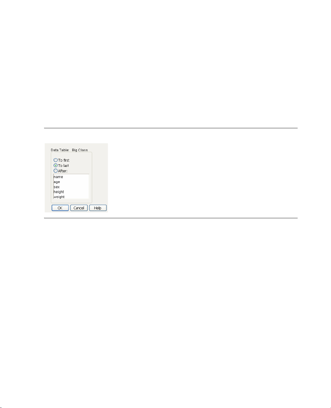
72 Entering, Editing, and Managing Data Chapter 3

Editing Data and Tables

Reordering Columns

You can rearrange, or sort data table columns by their name, data type, or modeling type, or you can reverse their current order. You can also move selected columns to a particular place in the data table. To reorder columns:

1. Select

Cols > Reorder Columns.

2. Make a selection from the submenu options, which include the following:

Move Selected Columns Moves the selected columns to a particular place in the data table. When you

select

Move Selected Columns, the Move Selected Columns window appears.

Figure 3.22 Move Selected Columns Window

The Move Selected Columns window contains the following choices:

•

To fir s t : Moves the selected columns so they are in the left-most position in the data table.

•

To las t : Moves the selected columns so they are in the right-most position in the data table.

• After: Moves the selected columns so they are after a column that you identify.

Original Order Returns the columns to the order they were in at the time the data table was last saved.

Reorder by Name Arranges the columns from left to right in alphabetical order by column name.

Reorder By Data Type Arranges the columns from left to right in alphabetic order by data type

(character, numeric, row state).

Reorder By Modeling Type Arranges the columns from left to right in alphabetic order by modeling type

(continuous, ordinal, nominal). Row state columns have no modeling type, and are shown last.

Reverse Order Reverses the order of the data table columns.

Chapter 3 Entering, Editing, and Managing Data 73

row context menu column context menu

Editing Data and Tables

Rows and Columns Context Menus

When you right-click in the row number area, or at the top of a column in the column name area, the context menus shown in Figure 3.23 appear. These menus give you quick access to selected

Columns menu commands. For details, see “The Rows Menu,” p. 421 and “Context Menu for Columns,”

p. 53.

Note: The Sort command in the context menu for columns gives you a quick way to sort a data table by a single column in ascending values of that column. Sort twice to have the column sorted in descending values. The context menu Sort command does not display a window with sort options.

Figure 3.23 Context Menus for Rows and Columns

Rows and

Copying, Cutting, and Pasting

You can copy or cut and paste in JMP data tables by selecting Edit > Copy or Edit > Cut, and then Edit >

Paste.

Data that you cut or copy to the clipboard can be pasted into data tables or other applications.

• If one cell is selected, apply to all selected rows. Likewise, if no rows are selected, columns. If you select both rows and columns, intersection.

•The

Edit commands affect all values in selected rows if no columns are selected. They affect all values in

selected columns (except the header field) if no rows are selected.

• When both rows and columns are selected, intersection of those rows and columns.

The

Copy and Paste commands in the Edit menu function as listed in Table 3.7:

Edit commands apply only to that cell. If no columns are selected, Edit commands

Edit commands apply to all selected

Copy copies the subset of cells defined by their

Edit commands affect the subset of cells defined by the

74 Entering, Editing, and Managing Data Chapter 3

Editing Data and Tables

Ta bl e 3 .7 Using Copy and Paste

Action Instructions

Cut highlighted rows,

Select

Edit > Cut.

columns, a single cell, or combination of cells from the active data table

Copy highlighted rows, columns, a single cell, or

Select

Edit > Copy. On the clipboard, fields are delimited by tab

characters and a return character indicates an end of row. combination of cells from the active data table to the clipboard

Copy using the first line of

Select

Edit > Copy With Column Names.

data as column headings

Paste information from the clipboard to the highlighted area in a JMP

Select

Edit > Paste. This command can be used with the Copy command

to duplicate rows, columns, or any subset of cells defined by highlighted

rows and columns. data table

Duplicate an entire row or column

Highlight the row or column to be duplicated and select

Then highlight an existing row or column to receive the values select

> Paste

Duplicate a subset of values Highlight the cells and select

or column to receive the values and select

highlight the same arrangement of rows and columns to receive the copied

values as originally contained them.

Edit > Copy.

Edit

Edit > Copy. Then highlight an existing row

Edit > Paste. You must

Transfer data from another application into a JMP data table by copying and pasting

Paste using the first line of data as column headings

• If you paste data with fewer rows into a destination with more rows, the source values recycle until all receiving rows are filled.

• If you paste more rows or columns than you have highlighted, the excess values are lost unless you are pasting to the end of a data table.

• If you highlight no rows or columns before you paste, rows and columns are added as needed.

First copy the data to the clipboard from within the other application. Then select

Edit > Paste to paste the values into JMP. Pasting

automatically creates rows and columns as needed.

Select

Edit > Paste With Column Names.

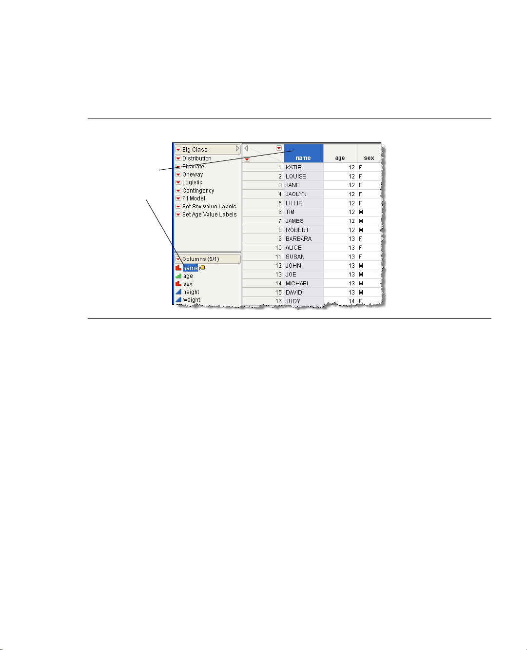
Chapter 3 Entering, Editing, and Managing Data 75

Click and drag column names in the data table or in the columns panel to move them.

Editing Data and Tables

Moving and Duplicating Values

Dragging and dropping is a convenient way to move or duplicate values in a data table.

Figure 3.24 Moving Columns

To move columns, cells, or rows:

1. In either the data table or in the columns panel, highlight the columns, cells, or rows that you want to move. To rearrange several columns, cells, or rows, press SHIFT and click, or press CTRL and click. Release the mouse.

2. Click the highlighted columns, cells, or rows and drag to the new position. If you do this with discontinuous columns, cells, or rows, they become contiguous when dropped. Note that when dragging and dropping cells:

– They retain all of their characteristics and column properties.

– They leave missing values in the original cells, and they replace the values at their destination if the

data types are the same.

– If you drag a set of cells to an empty area of the table, new columns are automatically created.

Also note that another way to move rows is to:

1. Highlight the rows that you want to move.

2. Select

Rows > Move Rows.

3. Specify where you would like to move the rows in the Move Rows window. Click the appropriate button to move highlighted rows to the beginning of the table ( after a specific row number (

After row:).

At start), to the end of the table (At end), or

76 Entering, Editing, and Managing Data Chapter 3

Editing Data and Tables

To duplicate columns, cells, or rows:

1. In either the data table or in the columns panel, highlight the columns, cells, or rows that you want to duplicate. To duplicate several columns, cells, or rows, hold down the SHIFT key and drag them to the new position.

2. Click the highlighted columns, cells, or rows and press the CTRL key and drag them to the new position. If you do this with discontinuous columns, cells, or rows, they become contiguous when dropped. Note that:

– The new columns have the original columns’ display format and their modeling types.

– If you drag a set of cells to an empty area of the table, new columns are automatically created. Your

values are copied to the destination, leaving the original values intact.

Using the Row Editor

The row editor lets you browse or edit cells one row at a time. You can access the row editor from an output report or from the data table. (See “Pasting Reports into Another Program,” p. 183.) To use the row editor from the data table:

1. Highlight a row in the data table.

2. Select

Rows > Row Editor or double-click a row.

Note: If you are inside of a plot instead of a data table, right-click inside the plot and select Row Editor to

access the row editor.

Figure 3.25 Row Editor

3. Edit the data. Note that if your data table contains value labels, the row editor displays the label, and when the cell is highlighted for editing, it shows the actual value. (See “Using Value Labels,” p. 151.)

4. Click the arrow buttons to browse through selected rows or the entire data set if no rows are selected. Table 3.8 describes the function of each button.

Ta bl e 3 .8 Row Editor Buttons

Shows the previous row.

Shows the previously selected row.

Chapter 3 Entering, Editing, and Managing Data 77

Editing Data and Tables

Ta bl e 3 .8 Row Editor Buttons (Continued)

Makes the row blink in graphs.

Shows the next selected row.

Shows the next row.

Enables you to search for a row. See “Selecting Cells That Contain Specific

Values,” p. 89.

Creates a new row at the end of the data table.

5. Click the red triangle icon in the row editor to select one of the following:

Next Selected Displays information for the selected row that is located after the current one.

Prev Selected Displays information for the selected row that is located before the current one.

Next Displays information for the row that is located after the current one, regardless of whether the

row is selected.

Prev Displays information for the row that is located before the current one, regardless of whether the

row is selected.

Save Saves the data table and any changes that you have made to it via the row editor.

New Row Creates a new row in the data table.

Find Displays the same window as if you had selected Rows > Row Selection > Select Where. Select

one of the options on the

Action on currently selected rows menu, and then highlight the column

whose rows you want to select. Type in the value for which you want JMP to search. See “Selecting

Cells with Specific Values,” p. 88, for details.

Blink Causes the current row’s highlight to flash at a rapid rate.

Note: Text in a locked column or a locked data table cannot be edited. See “Locking Columns,” p. 147, and

“Locking Tables,” p. 78, for details.

Changing Table Names

A data table’s name appears at the top of its window, in the table panel, and on all analysis reports. It is the name by which it has been or will be saved.

To change a table’s name:

1. Click twice on the table name in the table panel.

2. Type the name that you want.

On Windows, you can also change a data table’s name by selecting

Window > Set Title.

78 Entering, Editing, and Managing Data Chapter 3

Editing Data and Tables

Locking Tables

There are two ways you can lock a JMP data table:

• You can lock a table so that its values cannot be edited. However, you can still run analyses, assign characteristics, and so on. To do this, select

Figure 3.26 Lock the Table so Values Cannot be Edited

A lock icon appears next to the data table name. To unlock the file, select Lock Data Table again.

• You can lock a table so it can be edited but not saved. To do this, change the file’s properties according to your computer’s operating system. For example, change the file to be read-only. Then, when you open it in JMP, you see the words

Locked File in the table panel underneath the table’s name, as shown in

Figure 3.27.

Lock Data Table from the table panel menu (Figure 3.26).

Figure 3.27 A Locked File

If a file is locked in both ways described above, unlocking the file by selecting Lock Data Table from the table panel also removes the read-only setting.

Note: You can lock a column in place so when you scroll horizontally, the column remains visible. See

“Locking Columns in Place,” p. 143, for details.

Chapter 3 Entering, Editing, and Managing Data 79

Table variables

Editing Data and Tables

Adding Table Variables

Note: Starting in JMP 9, the Table Variable window is non-modal, meaning that you can access other windows and perform other operations while you are in the Table Variable window.

Table variables are character strings that are available to the entire table. They are any constant value that is always available in the data table. Table variable names are displayed in the table panel at the left of the data grid, as shown in Figure 3.28.

Figure 3.28 Table Variables are Located to the Left of the Data Grid

Table variables are mostly used to document tables. For example, when you installed JMP, a folder named

Sample Data was also installed. Many files in the Sample Data folder contain a table variable called Notes,

which contain descriptive information. The example in Figure 3.28 shows a data table that contains as one of its table variables. JMP also automatically creates table variables when you create a design table with the Design of Experiments commands in JMP. The design table has a table variable named with the name of the design type as its value.

Table variables can also be incorporated in formulas that you build using the formula editor. These formulas calculate values for a column by referring to a table variable. See “Referencing Columns and Table

Varia b l es,” p. 302, for details about constructing a formula that uses table variables.

Another use for table variables is to incorporate them into JSL scripts. See the Scripting Guide for details.

Adding New Table Variables

To add new table variables, proceed as follows:

1. In the tables panel, click the red triangle icon to the left of the data table name.

2. Select

New Table Variable. The Table Variable window appears.

3. Give the variable a name and value in the boxes labeled

Notes

Design

Name and Val ue, as shown in Figure 3.29.

80 Entering, Editing, and Managing Data Chapter 3

Editing Data and Tables

Figure 3.29 Naming and Defining the Table Variable

4. Click OK. The table variable appears in the tables panel.

Viewing or Editing Table Variables

1. Click twice on the content of an existing variable in the tables panel.

2. Edit its value.

Editing Table Variable Names

1. Double-click the table variable name. Or, right-click the table variable name and select window in Figure 3.29 appears.

2. Edit the name.

Deleting Table Variables

To delete a table variable, right-click its name or value and select

Example of Using a Table Variable

Table variables can be especially useful when you need to combine two or more data tables. For example, suppose two cancer trials were conducted at two different hospitals. One of the trials’ data is in a table called

Cancer1.jmp, and the other is in Cancer2.jmp.

Consolidate the data and the variables into one table, as follows:

1. Open the

Cancer1.jmp and Cancer2.jmp sample data tables.

Notice that there are two distinct table variables: Dosage Amount and Location.

2. From the

3. Select Cancer2 and click

4. Click

Cancer1.jmp data table, select Tables > Concatenate.

Add.

OK.

Edit. The

Delete.

Sas JMP User Manual

Specifications and Main Features

Frequently Asked Questions

User Manual

Preliminaries

Prerequisites

JMP Terminology

Learning about JMP

About JMP Documentation

Use JMP Help

Use Tutorials

Access Sample Data Tables

Conventions

Learn About Statistical and JSL Terms

Learn JMP Tips and Tricks

Access Resources on the Web

Common Features Throughout Platforms

Launch Window Features

Cast Selected Columns into Roles Buttons

Columns Filter Menu

Script Menus

Automatic Recalc Feature

Getting Started

Before You Start

The Tip of the Day Window

The JMP Home Window (Windows Only)

Work with Recent Files

Work with Open Windows

The JMP Starter Window

Display and Arrange Open Windows

Create New Data Tables

Open Existing JMP Files

Import Data

Open Text Files

Text Import Preview Options

Open a Text File in a Text Editing Window

Import Text from the Script Window

Open Remote Files and Web Pages

Open SPSS Files

Open Excel Files

Open SAS Data Sets

Create SAS Transport Files in SAS

E-mail Tables and Reports (Windows Only)

Encrypt and Decrypt Scripts

Entering, Editing, and Managing Data

Elements of JMP Data Tables

The Data Table Panels

The Table Panel

The Columns Panel

The Rows Panel

The Data Grid

Context Menu for Columns

Context Menu for Rows

Cursor Forms

Specifying Data Types and Modeling Types

About Data Types

About Modeling Types

How to Assign Data and Modeling Types

Using the Short-Integer Format

Choosing Numeric Formats

Numeric Format Options

Entering Data

Working With International Formats

Adding and Deleting Rows

Adding and Deleting Columns

Setting Up Initial Data Values

Filling Columns with Sequential Data

Entering Cell Formulas

Editing Data and Tables

Editing Cells

Editing Column Names

Recoding Data

Command Options

Viewing Patterns of Missing Data

Finding and Replacing Cell Values

Reordering Columns

Rows and Columns Context Menus

Copying, Cutting, and Pasting

Moving and Duplicating Values

Using the Row Editor