Sas DESIGN OF EXPERIMENTS RELEASE 9 User Manual

Download

Design of Experiments

Guide

Get the Most from JMP

Whether you are a first-time or a long-time user, there is always something to learn about JMP.

Visit JMP.com and to find the following:

• live and recorded Webcasts about how to get started with JMP

• video demos and Webcasts of new features and advanced techniques

• schedules for seminars being held in your area

• success stories showing how others use JMP

• a blog with tips, tricks, and stories from JMP staff

• a forum to discuss JMP with other users

http://www.jmp.com/getstarted/

Release 9

Design of Experiments

Guide

“The real voyage of discovery consists not in seeking new

landscapes, but in having new eyes.”

Marcel Proust

JMP, A Business Unit of SAS SAS Campus Drive Cary, NC 27513

The correct bibliographic citation for this manual is as follows: SAS Institute Inc. 2009. JMP® 9 Design of Experiments Guide, Second Edition. Cary, NC: SAS Institute Inc.

JMP

9 Design of Experiments Guide, Second Edition

ISBN 978-1-60764-597-9

For a hard-copy book: No part of this publication may be reproduced, stored in a retrieval system, or transmitted, in any form or by any means, electronic, mechanical, photocopying, or otherwise, without the prior written permission of the publisher, SAS Institute Inc.

For a Web download or e-book: Your use of this publication shall be governed by the terms established by the vendor at the time you acquire this publication.

U.S. Government Restricted Rights Notice: Use, duplication, or disclosure of this software and related documentation by the U.S. government is subject to the Agreement with SAS Institute and the restrictions set forth in FAR 52.227-19, Commercial Computer Software-Restricted Rights (June 1987).

SAS Institute Inc., SAS Campus Drive, Cary, North Carolina 27513.

1st printing, September 2010

JMP

, SAS® and all other SAS Institute Inc. product or service names are registered trademarks or

trademarks of SAS Institute Inc. in the USA and other countries. ® indicates USA registration.

Other brand and product names are registered trademarks or trademarks of their respective companies.

1 Introduction to Designing Experiments

A Beginner’s Tutorial . . . . . . . . . . . . . . . . . . . . . . . . . . . . . . . . . . . . . . . . . . . . . . . . . . . . . . . . . . . . 1

About Designing Experiments . . . . . . . . . . . . . . . . . . . . . . . . . . . . . . . . . . . . . . . . . . . . . . . . . . . . . . . . 3

My First Experiment . . . . . . . . . . . . . . . . . . . . . . . . . . . . . . . . . . . . . . . . . . . . . . . . . . . . . . . . . . . . . . . 3

The Situation . . . . . . . . . . . . . . . . . . . . . . . . . . . . . . . . . . . . . . . . . . . . . . . . . . . . . . . . . . . . . . . . . . 3

Step 1: Design the Experiment . . . . . . . . . . . . . . . . . . . . . . . . . . . . . . . . . . . . . . . . . . . . . . . . . . . . . 4

Step 2: Define Factor Constraints . . . . . . . . . . . . . . . . . . . . . . . . . . . . . . . . . . . . . . . . . . . . . . . . . . . 6

Step 3: Add Interaction Terms . . . . . . . . . . . . . . . . . . . . . . . . . . . . . . . . . . . . . . . . . . . . . . . . . . . . . 6

Step 4: Determine the Number of Runs . . . . . . . . . . . . . . . . . . . . . . . . . . . . . . . . . . . . . . . . . . . . . . 7

Step 5: Check the Design . . . . . . . . . . . . . . . . . . . . . . . . . . . . . . . . . . . . . . . . . . . . . . . . . . . . . . . . . 8

Step 6: Gather and Enter the Data . . . . . . . . . . . . . . . . . . . . . . . . . . . . . . . . . . . . . . . . . . . . . . . . . . 9

Step 7: Analyze the Results . . . . . . . . . . . . . . . . . . . . . . . . . . . . . . . . . . . . . . . . . . . . . . . . . . . . . . . 10

2 Examples Using the Custom Designer

. . . . . . . . . . . . . . . . . . . . . . . . . . . . . . . . . . . . . . . . . . . . . . . . . . . . . . . . . . . . . . . . . . . . . . . . . . . . . . 15

Creating Screening Experiments . . . . . . . . . . . . . . . . . . . . . . . . . . . . . . . . . . . . . . . . . . . . . . . . . . . . . . 17

Creating a Main-Effects-Only Screening Design . . . . . . . . . . . . . . . . . . . . . . . . . . . . . . . . . . . . . . 17

Creating a Screening Design to Fit All Two-Factor Interactions . . . . . . . . . . . . . . . . . . . . . . . . . . . 19

A Compromise Design Between Main Effects Only and All Interactions . . . . . . . . . . . . . . . . . . . . 20

Creating ‘Super’ Screening Designs . . . . . . . . . . . . . . . . . . . . . . . . . . . . . . . . . . . . . . . . . . . . . . . . 22

Screening Designs with Flexible Block Sizes . . . . . . . . . . . . . . . . . . . . . . . . . . . . . . . . . . . . . . . . . . 26

Checking for Curvature Using One Extra Run . . . . . . . . . . . . . . . . . . . . . . . . . . . . . . . . . . . . . . . . 30

Contents

Design of Experiments

Creating Response Surface Experiments . . . . . . . . . . . . . . . . . . . . . . . . . . . . . . . . . . . . . . . . . . . . . . . . 33

Exploring the Prediction Variance Surface . . . . . . . . . . . . . . . . . . . . . . . . . . . . . . . . . . . . . . . . . . . 33

Introducing I-Optimal Designs for Response Surface Modeling . . . . . . . . . . . . . . . . . . . . . . . . . . . 36

A Three-Factor Response Surface Design . . . . . . . . . . . . . . . . . . . . . . . . . . . . . . . . . . . . . . . . . . . . 37

Response Surface with a Blocking Factor . . . . . . . . . . . . . . . . . . . . . . . . . . . . . . . . . . . . . . . . . . . . 39

Creating Mixture Experiments . . . . . . . . . . . . . . . . . . . . . . . . . . . . . . . . . . . . . . . . . . . . . . . . . . . . . . . 43

Mixtures Having Nonmixture Factors . . . . . . . . . . . . . . . . . . . . . . . . . . . . . . . . . . . . . . . . . . . . . . 43

Experiments that are Mixtures of Mixtures . . . . . . . . . . . . . . . . . . . . . . . . . . . . . . . . . . . . . . . . . . . 47

Special-Purpose Uses of the Custom Designer . . . . . . . . . . . . . . . . . . . . . . . . . . . . . . . . . . . . . . . . . . . 50

Designing Experiments with Fixed Covariate Factors . . . . . . . . . . . . . . . . . . . . . . . . . . . . . . . . . . 50

Creating a Design with Two Hard-to-Change Factors: Split Plot . . . . . . . . . . . . . . . . . . . . . . . . . . . 54

Technical Discussion . . . . . . . . . . . . . . . . . . . . . . . . . . . . . . . . . . . . . . . . . . . . . . . . . . . . . . . . . . . . . . . 59

3 Building Custom Designs

The Basic Steps . . . . . . . . . . . . . . . . . . . . . . . . . . . . . . . . . . . . . . . . . . . . . . . . . . . . . . . . . . . . . . . . 63

Creating a Custom Design . . . . . . . . . . . . . . . . . . . . . . . . . . . . . . . . . . . . . . . . . . . . . . . . . . . . . . . . . . 65

Enter Responses and Factors into the Custom Designer . . . . . . . . . . . . . . . . . . . . . . . . . . . . . . . . . 65

Describe the Model . . . . . . . . . . . . . . . . . . . . . . . . . . . . . . . . . . . . . . . . . . . . . . . . . . . . . . . . . . . . 69

Specifying Alias Terms . . . . . . . . . . . . . . . . . . . . . . . . . . . . . . . . . . . . . . . . . . . . . . . . . . . . . . . . . . 70

Select the Number of Runs . . . . . . . . . . . . . . . . . . . . . . . . . . . . . . . . . . . . . . . . . . . . . . . . . . . . . . . 71

Understanding Design Evaluation . . . . . . . . . . . . . . . . . . . . . . . . . . . . . . . . . . . . . . . . . . . . . . . . . 72

Specify Output Options . . . . . . . . . . . . . . . . . . . . . . . . . . . . . . . . . . . . . . . . . . . . . . . . . . . . . . . . 78

Make the JMP Design Table . . . . . . . . . . . . . . . . . . . . . . . . . . . . . . . . . . . . . . . . . . . . . . . . . . . . . 79

Creating Random Block Designs . . . . . . . . . . . . . . . . . . . . . . . . . . . . . . . . . . . . . . . . . . . . . . . . . . . . . 80

Creating Split Plot Designs . . . . . . . . . . . . . . . . . . . . . . . . . . . . . . . . . . . . . . . . . . . . . . . . . . . . . . . . . 80

Creating Split-Split Plot Designs . . . . . . . . . . . . . . . . . . . . . . . . . . . . . . . . . . . . . . . . . . . . . . . . . . . . . . 81

Creating Strip Plot Designs . . . . . . . . . . . . . . . . . . . . . . . . . . . . . . . . . . . . . . . . . . . . . . . . . . . . . . . . . . 82

Special Custom Design Commands . . . . . . . . . . . . . . . . . . . . . . . . . . . . . . . . . . . . . . . . . . . . . . . . . . . . 83

Save Responses and Save Factors . . . . . . . . . . . . . . . . . . . . . . . . . . . . . . . . . . . . . . . . . . . . . . . . . . 84

Load Responses and Load Factors . . . . . . . . . . . . . . . . . . . . . . . . . . . . . . . . . . . . . . . . . . . . . . . . . . 85

Save Constraints and Load Constraints . . . . . . . . . . . . . . . . . . . . . . . . . . . . . . . . . . . . . . . . . . . . . . 85

Set Random Seed: Setting the Number Generator . . . . . . . . . . . . . . . . . . . . . . . . . . . . . . . . . . . . . . 85

Simulate Responses . . . . . . . . . . . . . . . . . . . . . . . . . . . . . . . . . . . . . . . . . . . . . . . . . . . . . . . . . . . . 86

Save X Matrix: Viewing the Number of Rows in the Moments Matrix and the Design Matrix (X) in the

Log . . . . . . . . . . . . . . . . . . . . . . . . . . . . . . . . . . . . . . . . . . . . . . . . . . . . . . . . . . . . . . . . . . . . . 87

Optimality Criterion . . . . . . . . . . . . . . . . . . . . . . . . . . . . . . . . . . . . . . . . . . . . . . . . . . . . . . . . . . . . 88

Number of Starts: Changing the Number of Random Starts . . . . . . . . . . . . . . . . . . . . . . . . . . . . . . 88

Sphere Radius: Constraining a Design to a Hypersphere . . . . . . . . . . . . . . . . . . . . . . . . . . . . . . . . 90

Disallowed Combinations: Accounting for Factor Level Restrictions . . . . . . . . . . . . . . . . . . . . . . . 90

Advanced Options for the Custom Designer . . . . . . . . . . . . . . . . . . . . . . . . . . . . . . . . . . . . . . . . . 92

Save Script to Script Window . . . . . . . . . . . . . . . . . . . . . . . . . . . . . . . . . . . . . . . . . . . . . . . . . . . . . 93

Assigning Column Properties . . . . . . . . . . . . . . . . . . . . . . . . . . . . . . . . . . . . . . . . . . . . . . . . . . . . . . . . 93

Define Low and High Values (DOE Coding) for Columns . . . . . . . . . . . . . . . . . . . . . . . . . . . . . . 94

Set Columns as Factors for Mixture Experiments . . . . . . . . . . . . . . . . . . . . . . . . . . . . . . . . . . . . . . 95

Define Response Column Values . . . . . . . . . . . . . . . . . . . . . . . . . . . . . . . . . . . . . . . . . . . . . . . . . . 96

Assign Columns a Design Role . . . . . . . . . . . . . . . . . . . . . . . . . . . . . . . . . . . . . . . . . . . . . . . . . . . . 97

Identify Factor Changes Column Property . . . . . . . . . . . . . . . . . . . . . . . . . . . . . . . . . . . . . . . . . . . 98

How Custom Designs Work: Behind the Scenes . . . . . . . . . . . . . . . . . . . . . . . . . . . . . . . . . . . . . . . . . 99

4 Screening Designs

. . . . . . . . . . . . . . . . . . . . . . . . . . . . . . . . . . . . . . . . . . . . . . . . . . . . . . . . . . . . . . . . . . . . . . . . . . . . . . 101

Screening Design Examples . . . . . . . . . . . . . . . . . . . . . . . . . . . . . . . . . . . . . . . . . . . . . . . . . . . . . . . . 103

Using Two Continuous Factors and One Categorical Factor . . . . . . . . . . . . . . . . . . . . . . . . . . . . 103

Using Five Continuous Factors . . . . . . . . . . . . . . . . . . . . . . . . . . . . . . . . . . . . . . . . . . . . . . . . . . . 105

Creating a Screening Design . . . . . . . . . . . . . . . . . . . . . . . . . . . . . . . . . . . . . . . . . . . . . . . . . . . . . . . . 109

Enter Responses . . . . . . . . . . . . . . . . . . . . . . . . . . . . . . . . . . . . . . . . . . . . . . . . . . . . . . . . . . . . . . 109

Enter Factors . . . . . . . . . . . . . . . . . . . . . . . . . . . . . . . . . . . . . . . . . . . . . . . . . . . . . . . . . . . . . . . . . 110

Choose a Design . . . . . . . . . . . . . . . . . . . . . . . . . . . . . . . . . . . . . . . . . . . . . . . . . . . . . . . . . . . . . . 111

Display and Modify a Design . . . . . . . . . . . . . . . . . . . . . . . . . . . . . . . . . . . . . . . . . . . . . . . . . . . . . 115

Specify Output Options . . . . . . . . . . . . . . . . . . . . . . . . . . . . . . . . . . . . . . . . . . . . . . . . . . . . . . . . . 119

View the Design Table . . . . . . . . . . . . . . . . . . . . . . . . . . . . . . . . . . . . . . . . . . . . . . . . . . . . . . . . . 120

Create a Plackett-Burman design . . . . . . . . . . . . . . . . . . . . . . . . . . . . . . . . . . . . . . . . . . . . . . . . . . . . 120

iii

Analysis of Screening Data . . . . . . . . . . . . . . . . . . . . . . . . . . . . . . . . . . . . . . . . . . . . . . . . . . . . . . . . . 122

Using the Screening Analysis Platform . . . . . . . . . . . . . . . . . . . . . . . . . . . . . . . . . . . . . . . . . . . . . . 123

Using the Fit Model Platform . . . . . . . . . . . . . . . . . . . . . . . . . . . . . . . . . . . . . . . . . . . . . . . . . . . . 124

5 Response Surface Designs

. . . . . . . . . . . . . . . . . . . . . . . . . . . . . . . . . . . . . . . . . . . . . . . . . . . . . . . . . . . . . . . . . . . . . . . . . . . . . 127

A Box-Behnken Design: The Tennis Ball Example . . . . . . . . . . . . . . . . . . . . . . . . . . . . . . . . . . . . . . . 129

The Prediction Profiler . . . . . . . . . . . . . . . . . . . . . . . . . . . . . . . . . . . . . . . . . . . . . . . . . . . . . . . . . . 132

A Response Surface Plot (Contour Profiler) . . . . . . . . . . . . . . . . . . . . . . . . . . . . . . . . . . . . . . . . . 134

Geometry of a Box-Behnken Design . . . . . . . . . . . . . . . . . . . . . . . . . . . . . . . . . . . . . . . . . . . . . . 136

Creating a Response Surface Design . . . . . . . . . . . . . . . . . . . . . . . . . . . . . . . . . . . . . . . . . . . . . . . . . . 136

Enter Responses and Factors . . . . . . . . . . . . . . . . . . . . . . . . . . . . . . . . . . . . . . . . . . . . . . . . . . . . . 137

Choose a Design . . . . . . . . . . . . . . . . . . . . . . . . . . . . . . . . . . . . . . . . . . . . . . . . . . . . . . . . . . . . . 137

Specify Output Options . . . . . . . . . . . . . . . . . . . . . . . . . . . . . . . . . . . . . . . . . . . . . . . . . . . . . . . . 139

View the Design Table . . . . . . . . . . . . . . . . . . . . . . . . . . . . . . . . . . . . . . . . . . . . . . . . . . . . . . . . . 140

6 Full Factorial Designs

. . . . . . . . . . . . . . . . . . . . . . . . . . . . . . . . . . . . . . . . . . . . . . . . . . . . . . . . . . . . . . . . . . . . . . . . . . . . . 143

The Five-Factor Reactor Example . . . . . . . . . . . . . . . . . . . . . . . . . . . . . . . . . . . . . . . . . . . . . . . . . . . . . 145

Analyze the Reactor Data . . . . . . . . . . . . . . . . . . . . . . . . . . . . . . . . . . . . . . . . . . . . . . . . . . . . . . . 146

Creating a Factorial Design . . . . . . . . . . . . . . . . . . . . . . . . . . . . . . . . . . . . . . . . . . . . . . . . . . . . . . . . . 151

Enter Responses and Factors . . . . . . . . . . . . . . . . . . . . . . . . . . . . . . . . . . . . . . . . . . . . . . . . . . . . . 151

Select Output Options . . . . . . . . . . . . . . . . . . . . . . . . . . . . . . . . . . . . . . . . . . . . . . . . . . . . . . . . . 152

Make the Table . . . . . . . . . . . . . . . . . . . . . . . . . . . . . . . . . . . . . . . . . . . . . . . . . . . . . . . . . . . . . . . 152

7 Mixture Designs

. . . . . . . . . . . . . . . . . . . . . . . . . . . . . . . . . . . . . . . . . . . . . . . . . . . . . . . . . . . . . . . . . . . . . . . . . . . . . . 155

Mixture Design Types . . . . . . . . . . . . . . . . . . . . . . . . . . . . . . . . . . . . . . . . . . . . . . . . . . . . . . . . . . . . . 157

The Optimal Mixture Design . . . . . . . . . . . . . . . . . . . . . . . . . . . . . . . . . . . . . . . . . . . . . . . . . . . . . . . 157

The Simplex Centroid Design . . . . . . . . . . . . . . . . . . . . . . . . . . . . . . . . . . . . . . . . . . . . . . . . . . . . . . . 158

Creating the Design . . . . . . . . . . . . . . . . . . . . . . . . . . . . . . . . . . . . . . . . . . . . . . . . . . . . . . . . . . . . 159

Simplex Centroid Design Examples . . . . . . . . . . . . . . . . . . . . . . . . . . . . . . . . . . . . . . . . . . . . . . . . 160

The Simplex Lattice Design . . . . . . . . . . . . . . . . . . . . . . . . . . . . . . . . . . . . . . . . . . . . . . . . . . . . . . . . . 161

The Extreme Vertices Design . . . . . . . . . . . . . . . . . . . . . . . . . . . . . . . . . . . . . . . . . . . . . . . . . . . . . . . . 163

Creating the Design . . . . . . . . . . . . . . . . . . . . . . . . . . . . . . . . . . . . . . . . . . . . . . . . . . . . . . . . . . . . 164

An Extreme Vertices Example with Range Constraints . . . . . . . . . . . . . . . . . . . . . . . . . . . . . . . . . 165

An Extreme Vertices Example with Linear Constraints . . . . . . . . . . . . . . . . . . . . . . . . . . . . . . . . . 167

Extreme Vertices Method: How It Works . . . . . . . . . . . . . . . . . . . . . . . . . . . . . . . . . . . . . . . . . . . 168

The ABCD Design . . . . . . . . . . . . . . . . . . . . . . . . . . . . . . . . . . . . . . . . . . . . . . . . . . . . . . . . . . . . . . . 168

Creating Ternary Plots . . . . . . . . . . . . . . . . . . . . . . . . . . . . . . . . . . . . . . . . . . . . . . . . . . . . . . . . . . . . . 169

Fitting Mixture Designs . . . . . . . . . . . . . . . . . . . . . . . . . . . . . . . . . . . . . . . . . . . . . . . . . . . . . . . . . . . . 170

Whole Model Tests and Analysis of Variance Reports . . . . . . . . . . . . . . . . . . . . . . . . . . . . . . . . . . 171

Understanding Response Surface Reports . . . . . . . . . . . . . . . . . . . . . . . . . . . . . . . . . . . . . . . . . . . 171

A Chemical Mixture Example . . . . . . . . . . . . . . . . . . . . . . . . . . . . . . . . . . . . . . . . . . . . . . . . . . . . . . . 171

Create the Design . . . . . . . . . . . . . . . . . . . . . . . . . . . . . . . . . . . . . . . . . . . . . . . . . . . . . . . . . . . . . 172

Analyze the Mixture Model . . . . . . . . . . . . . . . . . . . . . . . . . . . . . . . . . . . . . . . . . . . . . . . . . . . . . . 174

The Prediction Profiler . . . . . . . . . . . . . . . . . . . . . . . . . . . . . . . . . . . . . . . . . . . . . . . . . . . . . . . . . 175

The Mixture Profiler . . . . . . . . . . . . . . . . . . . . . . . . . . . . . . . . . . . . . . . . . . . . . . . . . . . . . . . . . . . 177

A Ternary Plot of the Mixture Response Surface . . . . . . . . . . . . . . . . . . . . . . . . . . . . . . . . . . . . . . 178

8 Discrete Choice Designs

. . . . . . . . . . . . . . . . . . . . . . . . . . . . . . . . . . . . . . . . . . . . . . . . . . . . . . . . . . . . . . . . . . . . . . . . . . . . . . 179

Introduction . . . . . . . . . . . . . . . . . . . . . . . . . . . . . . . . . . . . . . . . . . . . . . . . . . . . . . . . . . . . . . . . . . . . 181

Create an Example Choice Experiment . . . . . . . . . . . . . . . . . . . . . . . . . . . . . . . . . . . . . . . . . . . . . . . . 183

Analyze the Example Choice Experiment . . . . . . . . . . . . . . . . . . . . . . . . . . . . . . . . . . . . . . . . . . . . . . 186

Design a Choice Experiment Using Prior Information . . . . . . . . . . . . . . . . . . . . . . . . . . . . . . . . . . . . 189

Administer the Survey and Analyze Results . . . . . . . . . . . . . . . . . . . . . . . . . . . . . . . . . . . . . . . . . . . . . 191

Initial Choice Platform Analysis . . . . . . . . . . . . . . . . . . . . . . . . . . . . . . . . . . . . . . . . . . . . . . . . . . . 191

Find Unit Cost and Trade Off Costs with the Profiler . . . . . . . . . . . . . . . . . . . . . . . . . . . . . . . . . 192

9 Space-Filling Designs

. . . . . . . . . . . . . . . . . . . . . . . . . . . . . . . . . . . . . . . . . . . . . . . . . . . . . . . . . . . . . . . . . . . . . . . . . . . . . . 195

Introduction to Space-Filling Designs . . . . . . . . . . . . . . . . . . . . . . . . . . . . . . . . . . . . . . . . . . . . . . . . 197

Sphere-Packing Designs . . . . . . . . . . . . . . . . . . . . . . . . . . . . . . . . . . . . . . . . . . . . . . . . . . . . . . . . . . . 197

Creating a Sphere-Packing Design . . . . . . . . . . . . . . . . . . . . . . . . . . . . . . . . . . . . . . . . . . . . . . . . 197

Visualizing the Sphere-Packing Design . . . . . . . . . . . . . . . . . . . . . . . . . . . . . . . . . . . . . . . . . . . . . 199

Latin Hypercube Designs . . . . . . . . . . . . . . . . . . . . . . . . . . . . . . . . . . . . . . . . . . . . . . . . . . . . . . . . . . 200

Creating a Latin Hypercube Design . . . . . . . . . . . . . . . . . . . . . . . . . . . . . . . . . . . . . . . . . . . . . . . 200

Visualizing the Latin Hypercube Design . . . . . . . . . . . . . . . . . . . . . . . . . . . . . . . . . . . . . . . . . . . 202

Uniform Designs . . . . . . . . . . . . . . . . . . . . . . . . . . . . . . . . . . . . . . . . . . . . . . . . . . . . . . . . . . . . . . . . 204

Comparing Sphere-Packing, Latin Hypercube, and Uniform Methods . . . . . . . . . . . . . . . . . . . . . . . . 206

Minimum Potential Designs . . . . . . . . . . . . . . . . . . . . . . . . . . . . . . . . . . . . . . . . . . . . . . . . . . . . . . . . 207

Maximum Entropy Designs . . . . . . . . . . . . . . . . . . . . . . . . . . . . . . . . . . . . . . . . . . . . . . . . . . . . . . . . 209

Gaussian Process IMSE Optimal Designs . . . . . . . . . . . . . . . . . . . . . . . . . . . . . . . . . . . . . . . . . . . . . . . 211

Borehole Model: A Sphere-Packing Example . . . . . . . . . . . . . . . . . . . . . . . . . . . . . . . . . . . . . . . . . . . 212

Create the Sphere-Packing Design for the Borehole Data . . . . . . . . . . . . . . . . . . . . . . . . . . . . . . . 212

Guidelines for the Analysis of Deterministic Data . . . . . . . . . . . . . . . . . . . . . . . . . . . . . . . . . . . . 214

Results of the Borehole Experiment . . . . . . . . . . . . . . . . . . . . . . . . . . . . . . . . . . . . . . . . . . . . . . . 214

10 Accelerated Life Test Designs

Designing Experiments for Accelerated Life Tests . . . . . . . . . . . . . . . . . . . . . . . . . . . . . . . 219

Overview of Accelerated Life Test Designs . . . . . . . . . . . . . . . . . . . . . . . . . . . . . . . . . . . . . . . . . . . . . 221

Using the ALT Design Platform . . . . . . . . . . . . . . . . . . . . . . . . . . . . . . . . . . . . . . . . . . . . . . . . . . . . . 221

Platform Options . . . . . . . . . . . . . . . . . . . . . . . . . . . . . . . . . . . . . . . . . . . . . . . . . . . . . . . . . . . . . . . . 226

Example . . . . . . . . . . . . . . . . . . . . . . . . . . . . . . . . . . . . . . . . . . . . . . . . . . . . . . . . . . . . . . . . . . . . . . . 226

11 Nonlinear Designs

. . . . . . . . . . . . . . . . . . . . . . . . . . . . . . . . . . . . . . . . . . . . . . . . . . . . . . . . . . . . . . . . . . . . . . . . . . . . . . 231

Examples of Nonlinear Designs . . . . . . . . . . . . . . . . . . . . . . . . . . . . . . . . . . . . . . . . . . . . . . . . . . . . . 233

Using Nonlinear Fit to Find Prior Parameter Estimates . . . . . . . . . . . . . . . . . . . . . . . . . . . . . . . . 233

Creating a Nonlinear Design with No Prior Data . . . . . . . . . . . . . . . . . . . . . . . . . . . . . . . . . . . . . 239

Creating a Nonlinear Design . . . . . . . . . . . . . . . . . . . . . . . . . . . . . . . . . . . . . . . . . . . . . . . . . . . . . . . . 243

Identify the Response and Factor Column with Formula . . . . . . . . . . . . . . . . . . . . . . . . . . . . . . . . 243

Set Up Factors and Parameters in the Nonlinear Design Dialog . . . . . . . . . . . . . . . . . . . . . . . . . . 244

Enter the Number of Runs and Preview the Design . . . . . . . . . . . . . . . . . . . . . . . . . . . . . . . . . . . . 245

Make Table or Augment the Table . . . . . . . . . . . . . . . . . . . . . . . . . . . . . . . . . . . . . . . . . . . . . . . . 246

Advanced Options for the Nonlinear Designer . . . . . . . . . . . . . . . . . . . . . . . . . . . . . . . . . . . . . . . . . 247

12 Taguchi Designs

. . . . . . . . . . . . . . . . . . . . . . . . . . . . . . . . . . . . . . . . . . . . . . . . . . . . . . . . . . . . . . . . . . . . . . . . . . . . . 249

The Taguchi Design Approach . . . . . . . . . . . . . . . . . . . . . . . . . . . . . . . . . . . . . . . . . . . . . . . . . . . . . . 251

Taguchi Design Example . . . . . . . . . . . . . . . . . . . . . . . . . . . . . . . . . . . . . . . . . . . . . . . . . . . . . . . . . . . 251

Analyze the Data . . . . . . . . . . . . . . . . . . . . . . . . . . . . . . . . . . . . . . . . . . . . . . . . . . . . . . . . . . . . . . 254

Creating a Taguchi Design . . . . . . . . . . . . . . . . . . . . . . . . . . . . . . . . . . . . . . . . . . . . . . . . . . . . . . . . . 256

Detail the Response and Add Factors . . . . . . . . . . . . . . . . . . . . . . . . . . . . . . . . . . . . . . . . . . . . . . . 256

Choose Inner and Outer Array Designs . . . . . . . . . . . . . . . . . . . . . . . . . . . . . . . . . . . . . . . . . . . . . 257

Display Coded Design . . . . . . . . . . . . . . . . . . . . . . . . . . . . . . . . . . . . . . . . . . . . . . . . . . . . . . . . . . 258

Make the Design Table . . . . . . . . . . . . . . . . . . . . . . . . . . . . . . . . . . . . . . . . . . . . . . . . . . . . . . . . . 259

13 Augmented Designs

. . . . . . . . . . . . . . . . . . . . . . . . . . . . . . . . . . . . . . . . . . . . . . . . . . . . . . . . . . . . . . . . . . . . . . . . . . . . . . 261

A D-Optimal Augmentation of the Reactor Example . . . . . . . . . . . . . . . . . . . . . . . . . . . . . . . . . . . . . 263

Analyze the Augmented Design . . . . . . . . . . . . . . . . . . . . . . . . . . . . . . . . . . . . . . . . . . . . . . . . . . 266

Creating an Augmented Design . . . . . . . . . . . . . . . . . . . . . . . . . . . . . . . . . . . . . . . . . . . . . . . . . . . . . 274

Replicate a Design . . . . . . . . . . . . . . . . . . . . . . . . . . . . . . . . . . . . . . . . . . . . . . . . . . . . . . . . . . . . 274

Add Center Points . . . . . . . . . . . . . . . . . . . . . . . . . . . . . . . . . . . . . . . . . . . . . . . . . . . . . . . . . . . . 277

Creating a Foldover Design . . . . . . . . . . . . . . . . . . . . . . . . . . . . . . . . . . . . . . . . . . . . . . . . . . . . . . 278

Adding Axial Points . . . . . . . . . . . . . . . . . . . . . . . . . . . . . . . . . . . . . . . . . . . . . . . . . . . . . . . . . . . 279

Adding New Runs and Terms . . . . . . . . . . . . . . . . . . . . . . . . . . . . . . . . . . . . . . . . . . . . . . . . . . . 280

Special Augment Design Commands . . . . . . . . . . . . . . . . . . . . . . . . . . . . . . . . . . . . . . . . . . . . . . . . . . 283

Save the Design (X) Matrix . . . . . . . . . . . . . . . . . . . . . . . . . . . . . . . . . . . . . . . . . . . . . . . . . . . . . . 284

Modify the Design Criterion (D- or I- Optimality) . . . . . . . . . . . . . . . . . . . . . . . . . . . . . . . . . . . . 284

Select the Number of Random Starts . . . . . . . . . . . . . . . . . . . . . . . . . . . . . . . . . . . . . . . . . . . . . . . 285

Specify the Sphere Radius Value . . . . . . . . . . . . . . . . . . . . . . . . . . . . . . . . . . . . . . . . . . . . . . . . . . 285

Disallow Factor Combinations . . . . . . . . . . . . . . . . . . . . . . . . . . . . . . . . . . . . . . . . . . . . . . . . . . . 285

14 Prospective Sample Size and Power

. . . . . . . . . . . . . . . . . . . . . . . . . . . . . . . . . . . . . . . . . . . . . . . . . . . . . . . . . . . . . . . . . . . . . . . . . . . . . 287

Launching the Sample Size and Power Platform . . . . . . . . . . . . . . . . . . . . . . . . . . . . . . . . . . . . . . . . . 289

One-Sample and Two-Sample Means . . . . . . . . . . . . . . . . . . . . . . . . . . . . . . . . . . . . . . . . . . . . . . . . . 289

Single-Sample Mean . . . . . . . . . . . . . . . . . . . . . . . . . . . . . . . . . . . . . . . . . . . . . . . . . . . . . . . . . . . 291

Sample Size and Power Animation for One Mean . . . . . . . . . . . . . . . . . . . . . . . . . . . . . . . . . . . . 294

Two-Sample Means . . . . . . . . . . . . . . . . . . . . . . . . . . . . . . . . . . . . . . . . . . . . . . . . . . . . . . . . . . . 295

k-Sample Means . . . . . . . . . . . . . . . . . . . . . . . . . . . . . . . . . . . . . . . . . . . . . . . . . . . . . . . . . . . . . . . . . 296

One Sample Standard Deviation . . . . . . . . . . . . . . . . . . . . . . . . . . . . . . . . . . . . . . . . . . . . . . . . . . . . 298

One Sample Standard Deviation Example . . . . . . . . . . . . . . . . . . . . . . . . . . . . . . . . . . . . . . . . . . 299

One-Sample and Two-Sample Proportions . . . . . . . . . . . . . . . . . . . . . . . . . . . . . . . . . . . . . . . . . . . . . 300

One Sample Proportion . . . . . . . . . . . . . . . . . . . . . . . . . . . . . . . . . . . . . . . . . . . . . . . . . . . . . . . . 300

Two Sample Proportions . . . . . . . . . . . . . . . . . . . . . . . . . . . . . . . . . . . . . . . . . . . . . . . . . . . . . . . 302

Counts per Unit . . . . . . . . . . . . . . . . . . . . . . . . . . . . . . . . . . . . . . . . . . . . . . . . . . . . . . . . . . . . . . . . . 305

Counts per Unit Example . . . . . . . . . . . . . . . . . . . . . . . . . . . . . . . . . . . . . . . . . . . . . . . . . . . . . . . 306

Sigma Quality Level . . . . . . . . . . . . . . . . . . . . . . . . . . . . . . . . . . . . . . . . . . . . . . . . . . . . . . . . . . . . . . 307

Sigma Quality Level Example . . . . . . . . . . . . . . . . . . . . . . . . . . . . . . . . . . . . . . . . . . . . . . . . . . . . 307

Number of Defects Computation Example . . . . . . . . . . . . . . . . . . . . . . . . . . . . . . . . . . . . . . . . . 308

vii

Reliability Test Plan and Demonstration . . . . . . . . . . . . . . . . . . . . . . . . . . . . . . . . . . . . . . . . . . . . . . 308

Reliability Test Plan . . . . . . . . . . . . . . . . . . . . . . . . . . . . . . . . . . . . . . . . . . . . . . . . . . . . . . . . . . . 308

Reliability Demonstration . . . . . . . . . . . . . . . . . . . . . . . . . . . . . . . . . . . . . . . . . . . . . . . . . . . . . . . 311

Index

Design of Experiments . . . . . . . . . . . . . . . . . . . . . . . . . . . . . . . . . . . . . . . . . . . . . . . . . . . . . . . . 319

viii

Credits and Acknowledgments

Origin

JMP was developed by SAS Institute Inc., Cary, NC. JMP is not a part of the SAS System, though portions of JMP were adapted from routines in the SAS System, particularly for linear algebra and probability calculations. Version 1 of JMP went into production in October 1989.

Credits

JMP was conceived and started by John Sall. Design and development were done by John Sall, Chung-Wei Ng, Michael Hecht, Richard Potter, Brian Corcoran, Annie Dudley Zangi, Bradley Jones, Craige Hales, Chris Gotwalt, Paul Nelson, Xan Gregg, Jianfeng Ding, Eric Hill, John Schroedl, Laura Lancaster, Scott McQuiggan, Melinda Thielbar, Clay Barker, Peng Liu, Dave Barbour, Jeff Polzin, John Ponte, and Steve Amerige.

In the SAS Institute Technical Support division, Duane Hayes, Wendy Murphrey, Rosemary Lucas, Win LeDinh, Bobby Riggs, Glen Grimme, Sue Walsh, Mike Stockstill, Kathleen Kiernan, and Liz Edwards provide technical support.

Nicole Jones, Kyoko Keener, Hui Di, Joseph Morgan, Wenjun Bao, Fang Chen, Susan Shao, Yusuke Ono, Michael Crotty, Jong-Seok Lee, Tonya Mauldin, Audrey Ventura, Ani Eloyan, Bo Meng, and Sequola McNeill provide ongoing quality assurance. Additional testing and technical support are provided by Noriki Inoue, Kyoko Takenaka, and Masakazu Okada from SAS Japan.

Bob Hickey and Jim Borek are the release engineers.

The JMP books were written by Ann Lehman, Lee Creighton, John Sall, Bradley Jones, Erin Vang, Melanie Drake, Meredith Blackwelder, Diane Perhac, Jonathan Gatlin, Susan Conaghan, and Sheila Loring, with contributions from Annie Dudley Zangi and Brian Corcoran. Creative services and production was done by SAS Publications. Melanie Drake implemented the Help system.

Jon Weisz and Jeff Perkinson provided project management. Also thanks to Lou Valente, Ian Cox, Mark Bailey, and Malcolm Moore for technical advice.

Thanks also to Georges Guirguis, Warren Sarle, Gordon Johnston, Duane Hayes, Russell Wolfinger, Randall Tobias, Robert N. Rodriguez, Ying So, Warren Kuhfeld, George MacKensie, Bob Lucas, Warren Kuhfeld, Mike Leonard, and Padraic Neville for statistical R&D support. Thanks are also due to Doug Melzer, Bryan Wolfe, Vincent DelGobbo, Biff Beers, Russell Gonsalves, Mitchel Soltys, Dave Mackie, and Stephanie Smith, who helped us get started with SAS Foundation Services from JMP.

Acknowledgments

We owe special gratitude to the people that encouraged us to start JMP, to the alpha and beta testers of JMP, and to the reviewers of the documentation. In particular we thank Michael Benson, Howard

Yetter (d), Andy Mauromoustakos, Al Best, Stan Young, Robert Muenchen, Lenore Herzenberg, Ramon Leon, Tom Lange, Homer Hegedus, Skip Weed, Michael Emptage, Pat Spagan, Paul Wenz, Mike Bowen, Lori Gates, Georgia Morgan, David Tanaka, Zoe Jewell, Sky Alibhai, David Coleman, Linda Blazek, Michael Friendly, Joe Hockman, Frank Shen, J.H. Goodman, David Iklé, Barry Hembree, Dan Obermiller, Jeff Sweeney, Lynn Vanatta, and Kris Ghosh.

Also, we thank Dick DeVeaux, Gray McQuarrie, Robert Stine, George Fraction, Avigdor Cahaner, José Ramirez, Gudmunder Axelsson, Al Fulmer, Cary Tuckfield, Ron Thisted, Nancy McDermott, Veronica Czitrom, Tom Johnson, Cy Wegman, Paul Dwyer, DaRon Huffaker, Kevin Norwood, Mike Thompson, Jack Reese, Francois Mainville, and John Wass.

We also thank the following individuals for expert advice in their statistical specialties: R. Hocking and P. Spector for advice on effective hypotheses; Robert Mee for screening design generators; Roselinde Kessels for advice on choice experiments; Greg Piepel, Peter Goos, J. Stuart Hunter, Dennis Lin, Doug Montgomery, and Chris Nachtsheim for advice on design of experiments; Jason Hsu for advice on multiple comparisons methods (not all of which we were able to incorporate in JMP); Ralph O’Brien for advice on homogeneity of variance tests; Ralph O’Brien and S. Paul Wright for advice on statistical power; Keith Muller for advice in multivariate methods, Harry Martz, Wayne Nelson, Ramon Leon, Dave Trindade, Paul Tobias, and William Q. Meeker for advice on reliability plots; Lijian Yang and J.S. Marron for bivariate smoothing design; George Milliken and Yurii Bulavski for development of mixed models; Will Potts and Cathy Maahs-Fladung for data mining; Clay Thompson for advice on contour plotting algorithms; and Tom Little, Damon Stoddard, Blanton Godfrey, Tim Clapp, and Joe Ficalora for advice in the area of Six Sigma; and Josef Schmee and Alan Bowman for advice on simulation and tolerance design.

For sample data, thanks to Patrice Strahle for Pareto examples, the Texas air control board for the pollution data, and David Coleman for the pollen (eureka) data.

Translations

Trish O'Grady coordinates localization. Special thanks to Noriki Inoue, Kyoko Takenaka, Masakazu Okada, Naohiro Masukawa and Yusuke Ono (SAS Japan); and Professor Toshiro Haga (retired, Tokyo University of Science) and Professor Hirohiko Asano (Tokyo Metropolitan University) for reviewing our Japanese translation; Professors Fengshan Bai, Xuan Lu, and Jianguo Li at Tsinghua University in Beijing, and their assistants Rui Guo, Shan Jiang, Zhicheng Wan, and Qiang Zhao; and William Zhou (SAS China) and Zhongguo Zheng, professor at Peking University, for reviewing the Simplified Chinese translation; Jacques Goupy (consultant, ReConFor) and Olivier Nuñez (professor, Universidad Carlos III de Madrid) for reviewing the French translation; Dr. Byung Chun Kim (professor, Korea Advanced Institute of Science and Technology) and Duk-Hyun Ko (SAS Korea) for reviewing the Korean translation; Bertram Schäfer and David Meintrup (consultants, StatCon) for reviewing the German translation; Patrizia Omodei, Maria Scaccabarozzi, and Letizia Bazzani (SAS Italy) for reviewing the Italian translation. Finally, thanks to all the members of our outstanding translation teams.

Past Support

Many people were important in the evolution of JMP. Special thanks to David DeLong, Mary Cole, Kristin Nauta, Aaron Walker, Ike Walker, Eric Gjertsen, Dave Tilley, Ruth Lee, Annette Sanders, Tim Christensen, Eric Wasserman, Charles Soper, Wenjie Bao, and Junji Kishimoto. Thanks to SAS Institute quality assurance by Jeanne Martin, Fouad Younan, and Frank Lassiter. Additional testing for Versions 3 and 4 was done by Li Yang, Brenda Sun, Katrina Hauser, and Andrea Ritter.

Also thanks to Jenny Kendall, John Hansen, Eddie Routten, David Schlotzhauer, and James Mulherin. Thanks to Steve Shack, Greg Weier, and Maura Stokes for testing JMP Version 1.

Thanks for support from Charles Shipp, Harold Gugel (d), Jim Winters, Matthew Lay, Tim Rey, Rubin Gabriel, Brian Ruff, William Lisowski, David Morganstein, Tom Esposito, Susan West, Chris Fehily, Dan Chilko, Jim Shook, Ken Bodner, Rick Blahunka, Dana C. Aultman, and William Fehlner.

Technology License Notices

WARRANTIES WITH REGARD TO THIS SOFTWARE, INCLUDING ALL IMPLIED WARRANTIES OF MERCHANTABILITY AND FITNESS, IN NO EVENT SHALL NEIL HODGSON BE LIABLE FOR ANY SPECIAL, INDIRECT OR CONSEQUENTIAL DAMAGES OR ANY DAMAGES WHATSOEVER RESULTING FROM LOSS OF USE, DATA OR PROFITS, WHETHER IN AN ACTION OF CONTRACT, NEGLIGENCE OR OTHER TORTIOUS ACTION, ARISING OUT OF OR IN CONNECTION WITH THE USE OR PERFORMANCE OF THIS SOFTWARE.

TO THIS SOFTWARE, INCLUDING ALL IMPLIED WARRANTIES OF MERCHANTABILITY AND FITNESS, IN NO EVENT SHALL KEITH PACKARD BE LIABLE FOR ANY SPECIAL, INDIRECT OR CONSEQUENTIAL DAMAGES OR ANY DAMAGES WHATSOEVER RESULTING FROM LOSS OF USE, DATA OR PROFITS, WHETHER IN AN ACTION OF CONTRACT, NEGLIGENCE OR OTHER TORTIOUS ACTION, ARISING OUT OF OR IN CONNECTION WITH THE USE OR PERFORMANCE OF THIS SOFTWARE.

KEITH PACKARD DISCLAIMS ALL WARRANTIES WITH REGARD

NEIL HODGSON DISCLAIMS ALL

xii

Chapter 1

Introduction to Designing Experiments

A Beginner’s Tutorial

This tutorial chapter introduces you to the design of experiments (DOE) using JMP’s custom designer. It gives a general understanding of how to design an experiment using JMP. Refer to subsequent chapters in this book for more examples and procedures on how to design an experiment for your specific project.

Contents

About Designing Experiments. . . . . . . . . . . . . . . . . . . . . . . . . . . . . . . . . . . . . . . . . . . . . . . . . . . . . . . . . . 3

My First Experiment . . . . . . . . . . . . . . . . . . . . . . . . . . . . . . . . . . . . . . . . . . . . . . . . . . . . . . . . . . . . . . . . . 3

The Situation . . . . . . . . . . . . . . . . . . . . . . . . . . . . . . . . . . . . . . . . . . . . . . . . . . . . . . . . . . . . . . . . . . . 3

Step 1: Design the Experiment . . . . . . . . . . . . . . . . . . . . . . . . . . . . . . . . . . . . . . . . . . . . . . . . . . . . . . 4

Step 2: Define Factor Constraints . . . . . . . . . . . . . . . . . . . . . . . . . . . . . . . . . . . . . . . . . . . . . . . . . . . . 6

Step 3: Add Interaction Terms . . . . . . . . . . . . . . . . . . . . . . . . . . . . . . . . . . . . . . . . . . . . . . . . . . . . . . . 6

Step 4: Determine the Number of Runs . . . . . . . . . . . . . . . . . . . . . . . . . . . . . . . . . . . . . . . . . . . . . . . 7

Step 5: Check the Design . . . . . . . . . . . . . . . . . . . . . . . . . . . . . . . . . . . . . . . . . . . . . . . . . . . . . . . . . . 8

Step 6: Gather and Enter the Data . . . . . . . . . . . . . . . . . . . . . . . . . . . . . . . . . . . . . . . . . . . . . . . . . . . 9

Step 7: Analyze the Results . . . . . . . . . . . . . . . . . . . . . . . . . . . . . . . . . . . . . . . . . . . . . . . . . . . . . . . . .10

Chapter 1 Introduction to Designing Experiments 3

About Designing Experiments

Increasing productivity and improving quality are important goals in any business. The methods for determining how to increase productivity and improve quality are evolving. They have changed from costly and time-consuming trial-and-error searches to the powerful, elegant, and cost-effective statistical methods that JMP provides.

Designing experiments in JMP is centered around factors, responses, a model, and runs. JMP helps you determine if and how a factor affects a response.

My First Experiment

If you have never used JMP to design an experiment, this section shows you how to design the experiment and how to understand JMP’s output.

Tip: The recommended way to create an experiment is to use the custom designer. JMP also provides classical designs for use in textbook situations.

The Situation

Your goal is to find the best way to microwave a bag of popcorn. Because you have some experience with this, it is easy to decide on reasonable ranges for the important factors:

• how long to cook the popcorn (between 3 and 5 minutes)

• what level of power to use on the microwave oven (between settings 5 and 10)

• which brand of popcorn to use (Top Secret or Wilbur)

When a bag of popcorn is popped, most of the kernels pop, but some remain unpopped. You prefer to have all (or nearly all) of the kernels popped and no (or very few) unpopped kernels. Therefore, you define “the best popped bag” based on the ratio of popped kernels to the total number of kernels.

A good way to improve any procedure is to conduct an experiment. For each experimental run, JMP’s custom designer determines which brand to use, how long to cook each bag in the microwave and what power setting to use. Each run involves popping one bag of corn. After popping a bag, enter the total number of kernels and the number of popped kernels into the appropriate row of a JMP data table. After doing all the experimental runs, use JMP’s model fitting capabilities to do the data analysis. Then, you can use JMP’s profiling tools to determine the optimal settings of popping time, power level, and brand.

4 Introduction to Designing Experiments Chapter 1

My First Experiment

Step 1: Design the Experiment

The first step is to select DOE > Custom Design. Then, define the responses and factors.

Define the Responses: Popped Kernels and Total Kernels

There are two responses in this experiment:

• the number of popped kernels

• the total number of kernels in the bag. After popping the bag add the number of unpopped kernels to the number of popped kernels to get the total number of kernels in the bag.

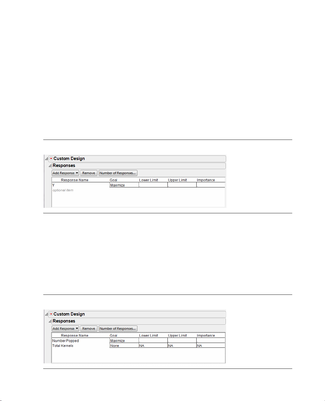
By default, the custom designer contains one response labeled

Figure 1.1 Custom Design Responses Panel

Y (Figure 1.1).

You want to add a second response to the Responses panel and change the names to be more descriptive:

1. To rename the increase the number of popped kernels, leave the goal at

2. To add the second response (total number of kernels), click menu that appears. JMP labels this response

3. Double-click

Y response, double-click the name and type “Number Popped.” Since you want to

Maximize.

Add Response and choose None from the

Y2 by default.

Y2 and type “Total Kernels” to rename it.

The completed Responses panel looks like Figure 1.2.

Figure 1.2 Renamed Responses with Specified Goals

Chapter 1 Introduction to Designing Experiments 5

My First Experiment

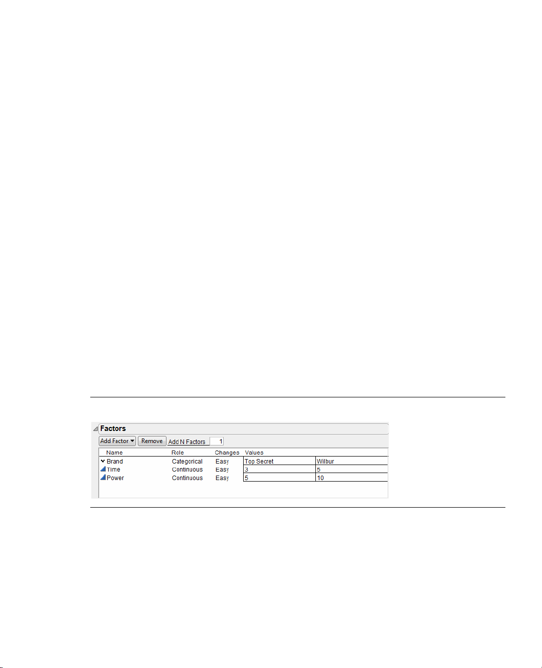
Define the Factors: Time, Power, and Brand

In this experiment, the factors are:

• brand of popcorn (Top Secret or Wilbur)

• cooking time for the popcorn (3 or 5 minutes)

• microwave oven power level (setting 5 or 10)

In the Factors panel, add

1. Click

Add Factor and select Categorical > 2 Level.

Brand as a two-level categorical factor:

2. To change the name of the factor (currently named

3. To rename the default levels (

Add

Time as a two-level continuous factor:

4. Click

Add Factor and select Continuous.

5. Change the default name of the factor (

6. Likewise, to rename the default levels (

L1 and L2), click the level names and type Top S ec r e t and Wilbur.

X2) by double-clicking it and typing Time.

–1 and 1) as 3 and 5, click the current level name and type in the

new value.

Add

Power as a two-level continuous factor:

7. Click

8. Change the name of the factor (currently named

9. Rename the default levels (currently named

Add Factor and select Continuous.

X3) by double-clicking it and typing Power.

-1 and 1) as 5 and 10 by clicking the current name and

typing. The completed Factors panel looks like Figure 1.3.

Figure 1.3 Renamed Factors with Specified Values

X1), double-click on its name and type Brand.

10. Click Continue.

6 Introduction to Designing Experiments Chapter 1

My First Experiment

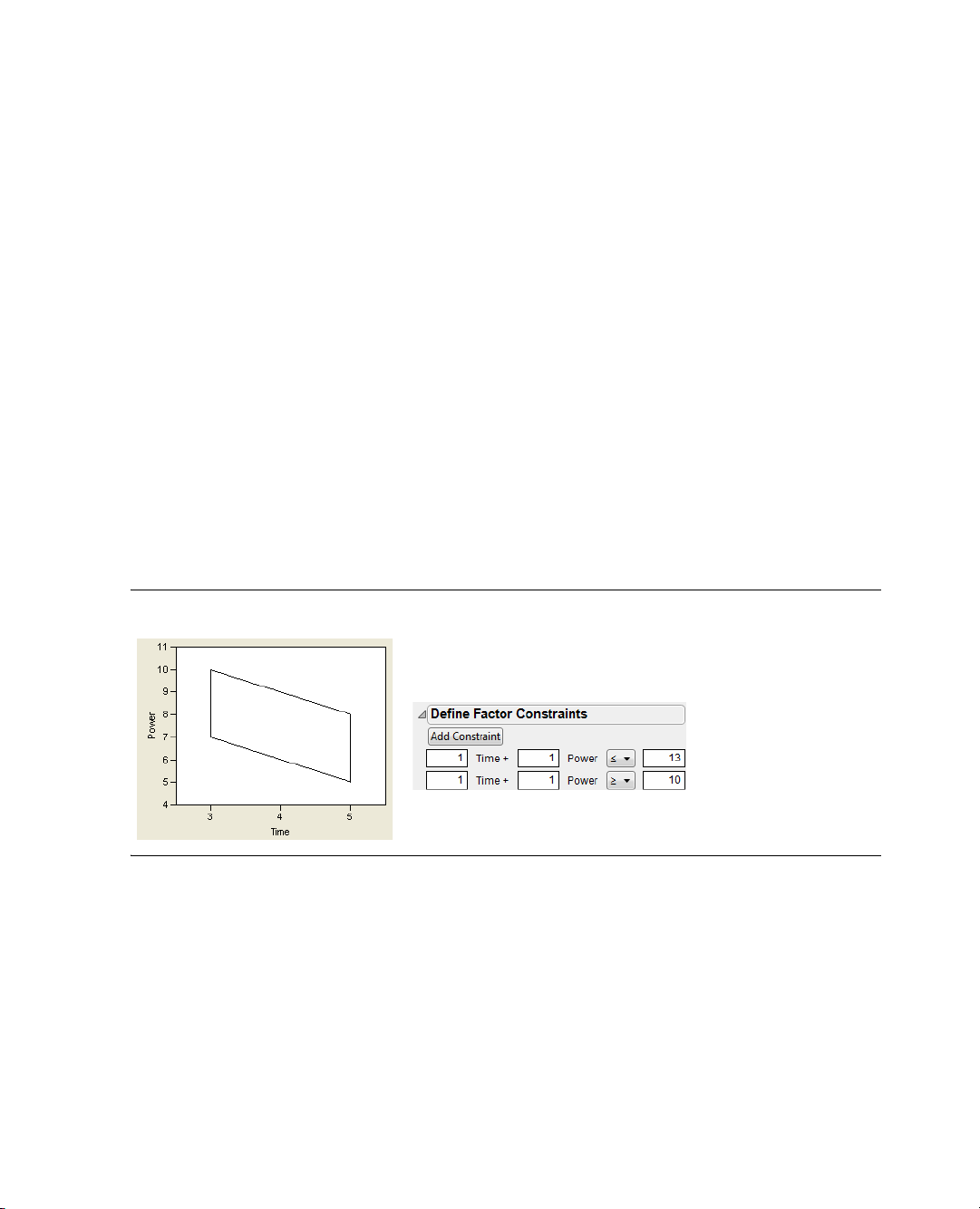
Step 2: Define Factor Constraints

The popping time for this experiment is either 3 or 5 minutes, and the power settings on the microwave are 5 and 10. From experience, you know that

• popping corn for a long time on a high setting tends to scorch kernels.

• not many kernels pop when the popping time is brief and the power setting is low.

You want to constrain the combined popping time and power settings to be less than or equal to 13, but greater than or equal to 10. To define these limits:

1. Open the Constraints panel by clicking the disclosure button beside the

Define Factor Constraints title

bar (see Figure 1.4).

2. Click the

Add Constraint button twice, once for each of the known constraints.

3. Complete the information, as shown to the right in Figure 1.4. These constraints tell the Custom Designer to avoid combinations of to change

<= to >= in the second constraint.

Power and Time that sum to less than 10 and more than 13. Be sure

The area inside the parallelogram, illustrated on the left in Figure 1.4, is the allowable region for the runs. You can see that popping for 5 minutes at a power of 10 is not allowed and neither is popping for 3 minutes at a power of 5.

Figure 1.4 Defining Factor Constraints

Step 3: Add Interaction Terms

You are interested in the possibility that the effect of any factor on the proportion of popped kernels may depend on the value of some other factor. For example, the effect of a change in popping time for the Wilbur popcorn brand could be larger than the same change in time for the Top Secret brand. This kind of synergistic effect of factors acting in concert is called a two-factor interaction. You can examine all possible two-factor interactions in your a priori model of the popcorn popping process.

1. Click

Interactions in the Model panel and select 2nd. JMP adds two-factor interactions to the model as

shown to the left in Figure 1.5.

Chapter 1 Introduction to Designing Experiments 7

My First Experiment

In addition, you suspect the graph of the relationship between any factor and any response might be curved. You can see whether this kind of curvature exists with a quadratic model formed by adding the second order powers of effects to the model, as follows.

2. Click

Powers and select 2nd to add quadratic effects of the continuous factors, Power and Time.

The completed Model should look like the one to the right in Figure 1.5.

Figure 1.5 Add Interaction and Power Terms to the Model

Step 4: Determine the Number of Runs

The Design Generation panel in Figure 1.6 shows the minimum number of runs needed to perform the experiment with the effects you’ve added to the model. You can use that minimum or the default number of runs, or you can specify your own number of runs as long as that number is more than the minimum. JMP has no restrictions on the number of runs you request. For this example, use the default number of runs, 16. Click

Make Design to continue.

Figure 1.6 Model and Design Generation Panels

8 Introduction to Designing Experiments Chapter 1

My First Experiment

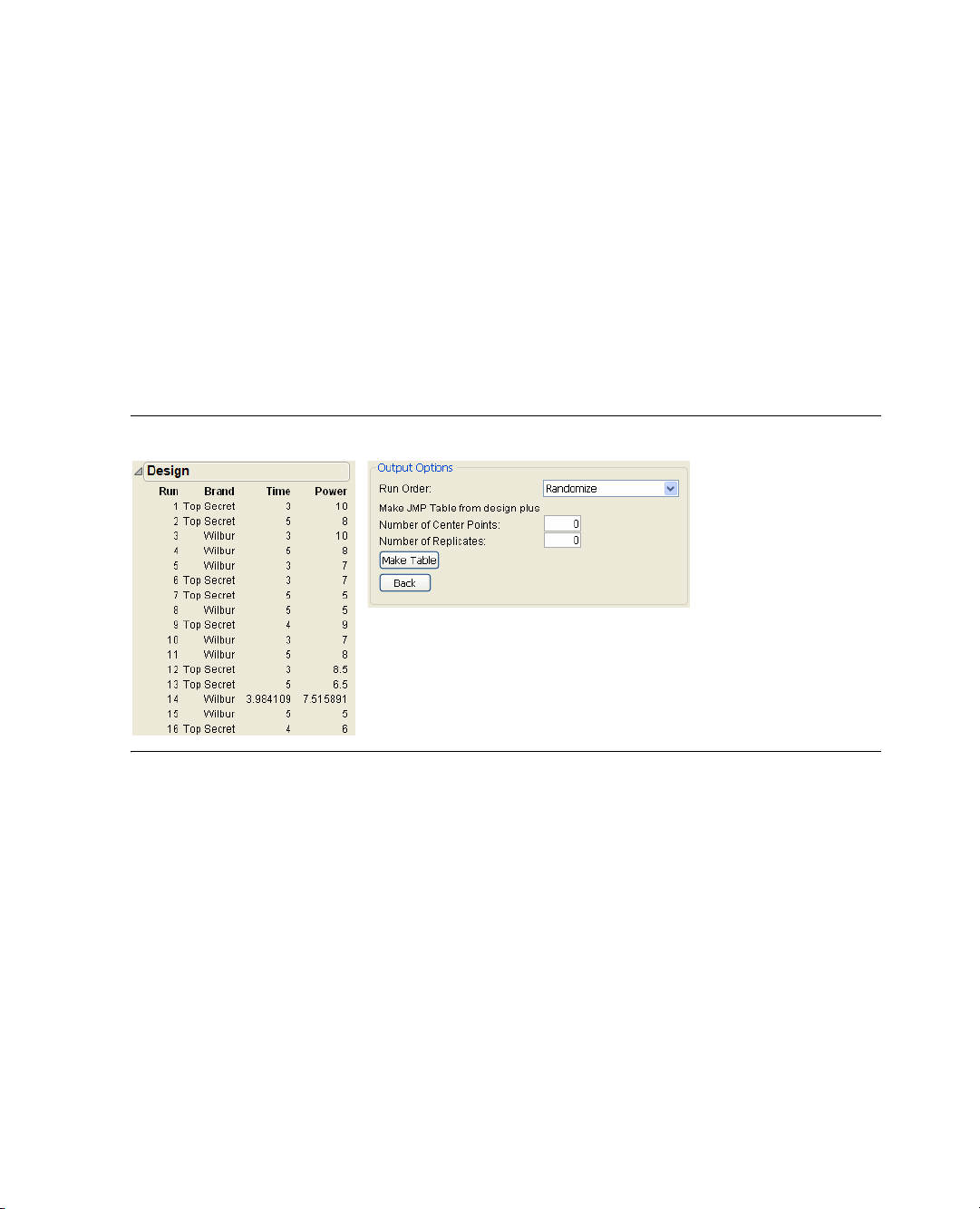
Step 5: Check the Design

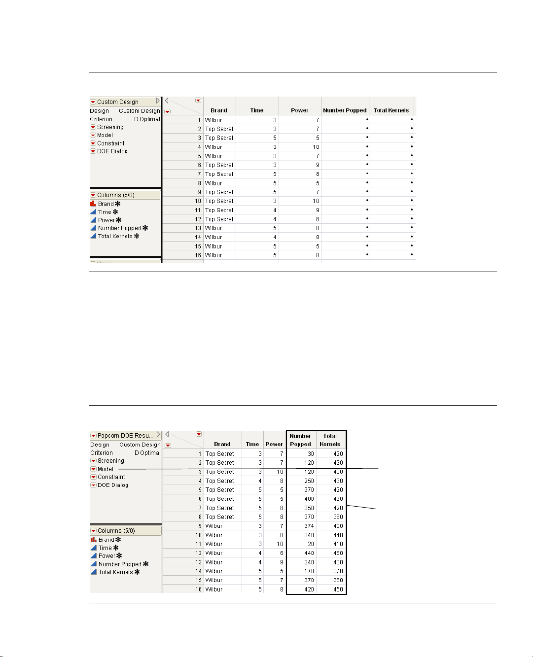
When you click Make Design, JMP generates and displays a design, as shown on the left in Figure 1.7. Note that because JMP uses a random seed to generate custom designs and there is no unique optimal design for this problem, your table may be different than the one shown here. You can see in the table that the custom design requires 8 runs using each brand of popcorn.

Scroll to the bottom of the Custom Design window and look at the Output Options area (shown to the right in Figure 1.7. The data table when it is created. Keep the selection at in a random order.

Run Order option lets you designate the order you want the runs to appear in the

Randomize so the rows (runs) in the output table appear

Now click

Figure 1.7 Design and Output Options Section of Custom Designer

Make Table in the Output Options section.

The resulting data table (Figure 1.8) shows the order in which you should do the experimental runs and provides columns for you to enter the number of popped and total kernels.

You do not have fractional control over the power and time settings on a microwave oven, so you should round the power and time settings, as shown in the data table. Although this altered design is slightly less optimal than the one the custom designer suggested, the difference is negligible.

Tip: Note that optionally, before clicking

Right

in the Run Order menu to have JMP present the results in the data table according to the brand. We

have conducted this experiment for you and placed the results, called

Sample Data folder installed with JMP. These results have the columns sorted from left to right.

Make Table in the Output Options, you could select Sort Left to

Popcorn DOE Results.jmp, in the

Chapter 1 Introduction to Designing Experiments 9

results from experiment

scripts to analyze data

My First Experiment

Figure 1.8 JMP Data Table of Design Runs Generated by Custom Designer

Step 6: Gather and Enter the Data

Pop the popcorn according to the design JMP provided. Then, count the number of popped and unpopped kernels left in each bag. Finally, enter the numbers shown below into the appropriate columns of the data table.

We have conducted this experiment for you and placed the results in the JMP. To see the results, open

data.

The data table is shown in Figure 1.9.

Figure 1.9 Results of the Popcorn DOE Experiment

Popcorn DOE Results.jmp from the Design Experiment folder in the sample

Sample Data folder installed with

10 Introduction to Designing Experiments Chapter 1

My First Experiment

Step 7: Analyze the Results

After the experiment is finished and the number of popped kernels and total kernels have been entered into the data table, it is time to analyze the data. The design data table has a script, labeled the top left panel of the table. When you created the design, a standard least squares analysis was stored in the

Model script with the data table.

Model, that shows in

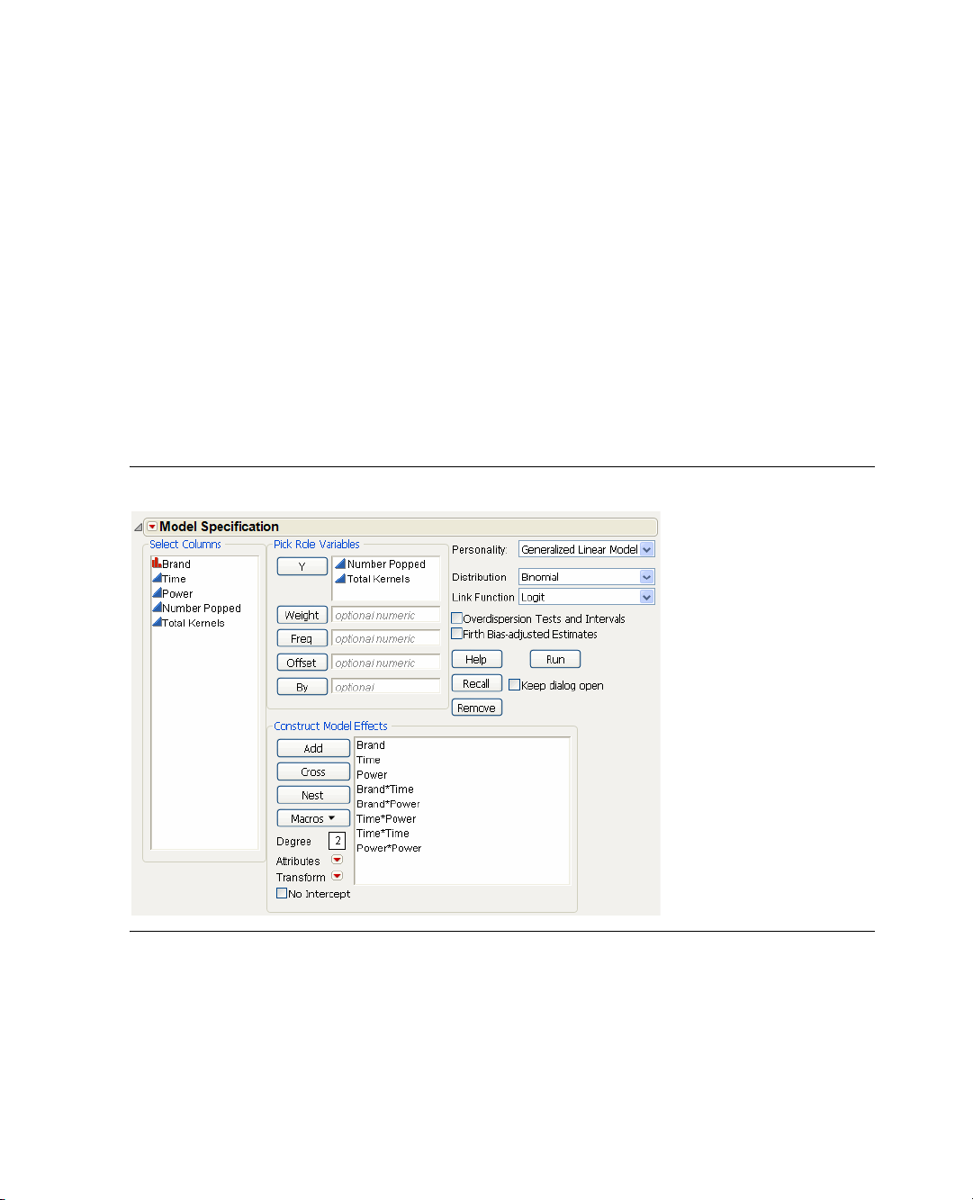
1. Click the red triangle for

The default fitting personality in the model dialog is

Model and select Run Script.

Standard Least Squares. One assumption of

standard least squares is that your responses are normally distributed. But because you are modeling the proportion of popped kernels it is more appropriate to assume that your responses come from a binomial distribution. You can use this assumption by changing to a generalized linear model.

2. Change the Personality to

Logit, as shown in Figure 1.10.

Figure 1.10 Fitting the Model

Generalized Linear Model, Distribution to Binomial, and Link Function to

3. Click Run.

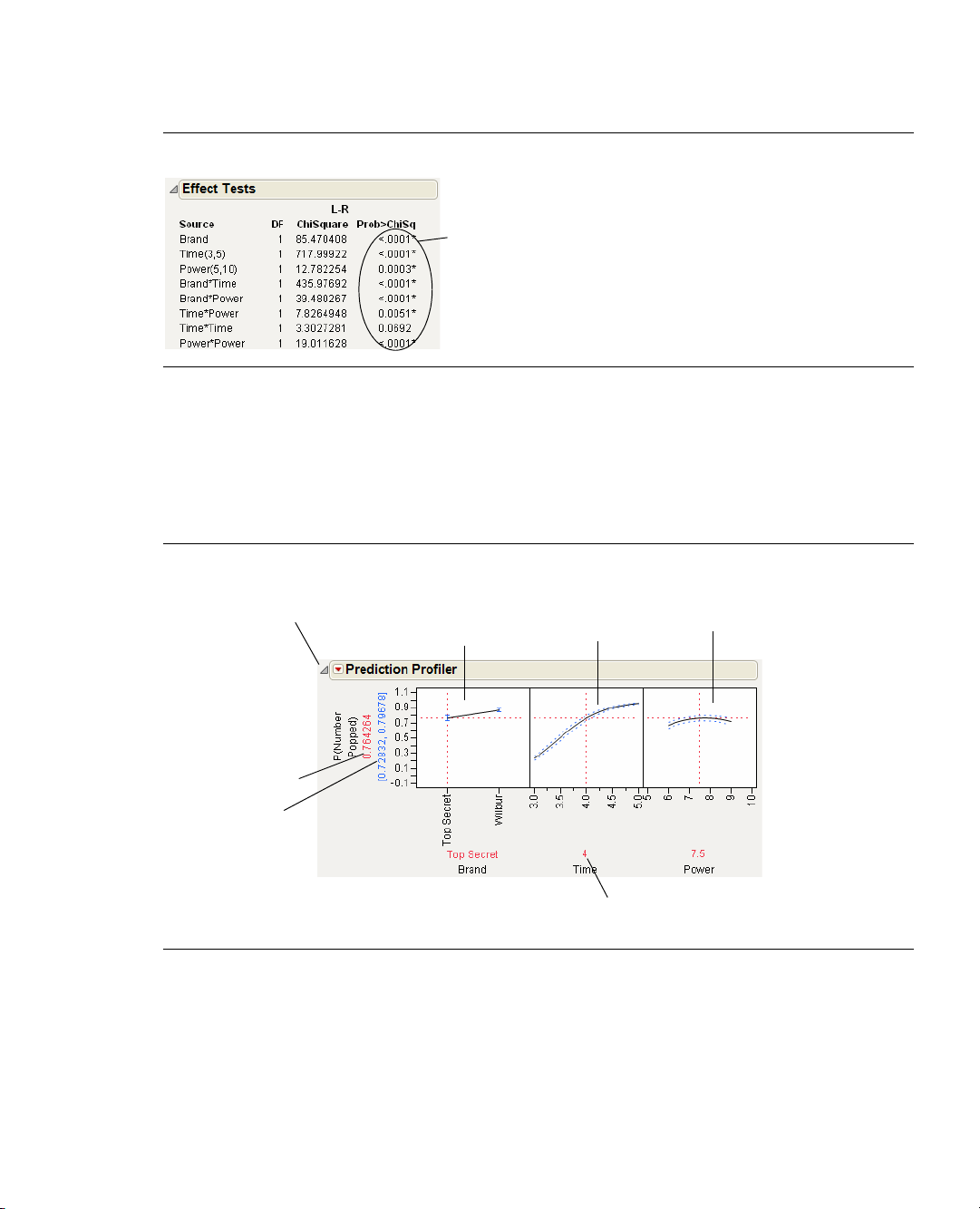
4. Scroll down to view the Effect Tests table (Figure 1.11) and look in the column labeled Prob>Chisq. This column lists p-values. A low p-value (a value less than 0.05) indicates that results are statistically significant. There are asterisks that identify the low p-values. You can therefore conclude that, in this experiment, all the model effects except for there is a strong relationship between popping time ( (

Brand), and the proportion of popped kernels.

Time*Time are highly significant. You have confirmed that

Time), microwave setting (Power), popcorn brand

Chapter 1 Introduction to Designing Experiments 11

p-values indicate significance. Values with * beside them are p-values that indicate the results are statistically significant.

Prediction trace for

Brand

predicted value of the response

95% confidence interval on the mean response

Factor values (here, time = 4)

Prediction trace for

Time

Prediction trace for

Power

Disclosure icon to open or close the Prediction Profiler

My First Experiment

Figure 1.11 Investigating p-Values

To further investigate, use the Prediction Profiler to see how changes in the factor settings affect the numbers of popped and unpopped kernels:

1. Choose

Profilers > Profiler from the red triangle menu on the Generalized Linear Model Fit title bar.

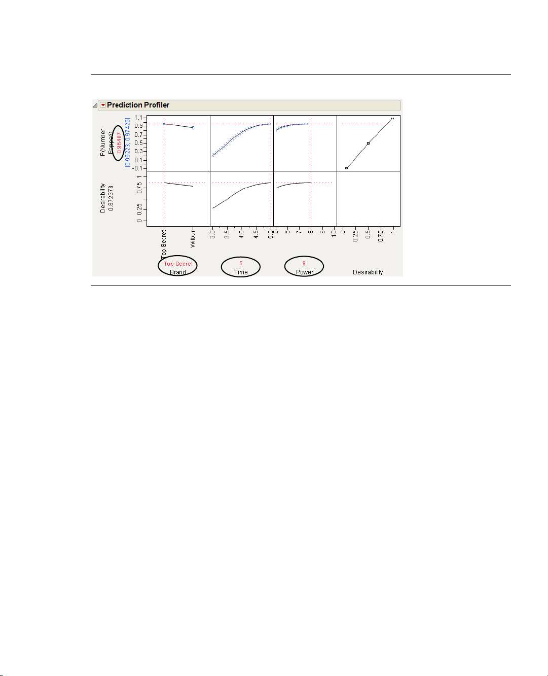
The Prediction Profiler is shown at the bottom of the report. Figure 1.12 shows the Prediction Profiler for the popcorn experiment. Prediction traces are displayed for each factor.

Figure 1.12 The Prediction Profiler

2. Move the vertical red dotted lines to see the effect that changing a factor value has on the response. For example, drag the red line in the

Time graph to the right and left (Figure 1.13).

12 Introduction to Designing Experiments Chapter 1

My First Experiment

Figure 1.13 Moving the Time Value from 4 to Near 5

As Time increases and decreases, the curved Time and Power prediction traces shift their slope and maximum/minimum values. The substantial slope shift tells you there is an interaction (synergistic effect) involving

Time and Power.

Furthermore, the steepness of a prediction trace reveals a factor’s importance. Because the prediction trace for

Time is steeper than that for Brand or Power (see Figure 1.13), you can see that cooking time is more

important than the brand of popcorn or the microwave power setting.

Now for the final steps.

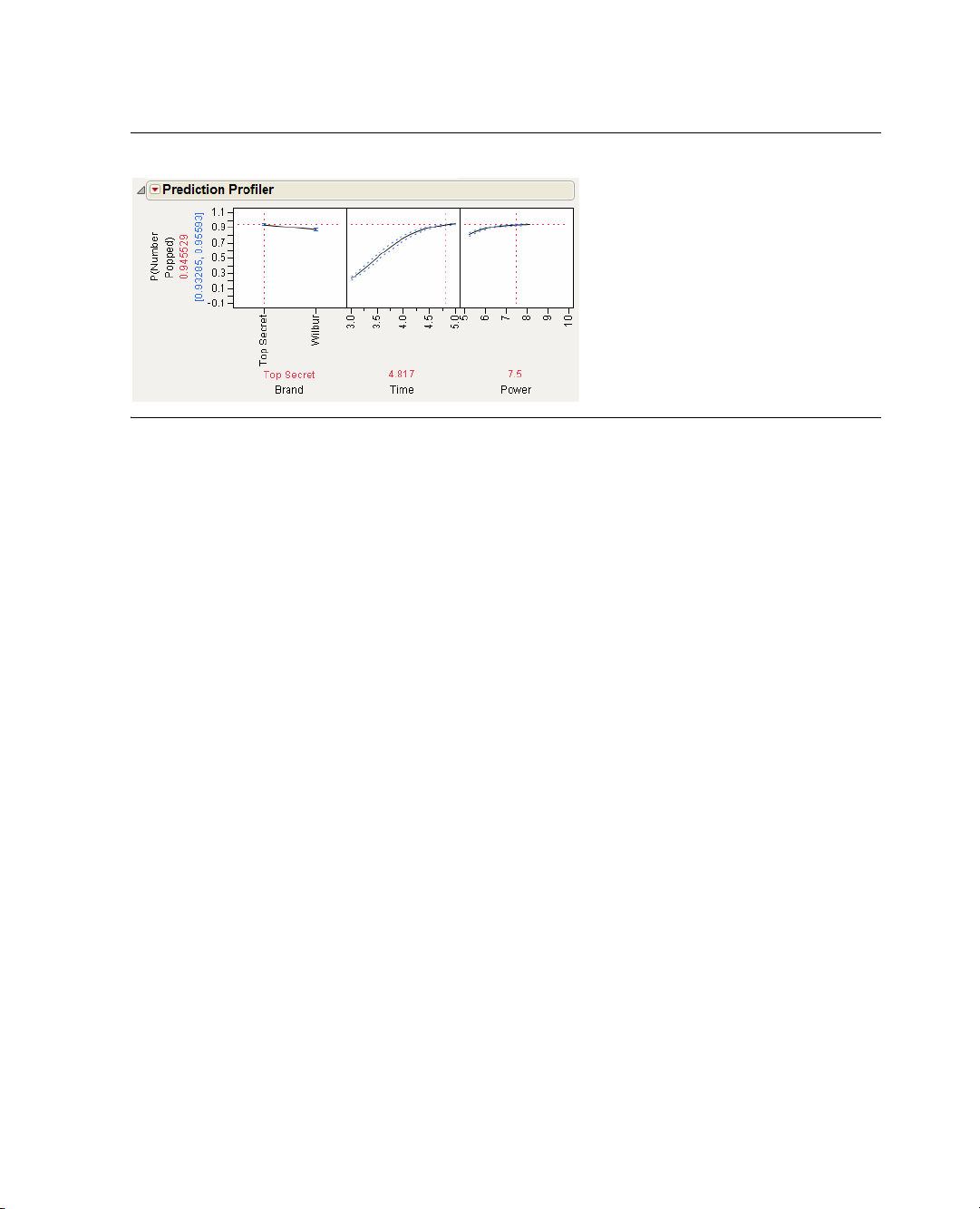
3. Click the red triangle icon in the Prediction Profiler title bar and select

4. Click the red triangle icon in the Prediction Profiler title bar and select

Desirability Functions.

Maximize Desirability. JMP

automatically adjusts the graph to display the optimal settings at which the most kernels will be popped (Figure 1.14).

Our experiment found how to cook the bag of popcorn with the greatest proportion of popped kernels: use Top Secret, cook for five minutes, and use a power level of 8. The experiment predicts that cooking at these settings will yield greater than 96.5% popped kernels.

Chapter 1 Introduction to Designing Experiments 13

My First Experiment

Figure 1.14 The Most Desirable Settings

The best settings are the Top Secret brand, cooking time at 5, and power set at 8.

14 Introduction to Designing Experiments Chapter 1

My First Experiment

Chapter 2

Describe Design Collect Fit Predict

Key mathematical steps: appropriate computer-based tools are empowering.

Key engineering steps: process knowledge and engineering judgement are important.

Identify factors and responses.

Compute design for maximum information from runs.

Use design to set factors: measure response for each run.

Compute best fit of mathematical model to data from test runs.

Use model to find best factor settings for on-target responses and minimum variability.

Examples Using the Custom Designer

The use of statistical methods in industry is increasing. Arguably, the most cost-beneficial of these methods for quality and productivity improvement is statistical design of experiments. A trial-and -error search for the vital few factors that most affect quality is costly and time-consuming. The purpose of experimental design is to characterize, predict, and then improve the behavior of any system or process. Designed experiments are a cost-effective way to accomplish these goals.

JMP’s custom designer is the recommended way to describe your process and create a design that works for your situation. To use the custom designer, you first enter the process variables and constraints, then JMP tailors a design to suit your unique case. This approach is more general and requires less experience and expertise than previous tools supporting the statistical design of experiments.

Custom designs accommodate any number of factors of any type. You can also control the number of experimental runs. This makes custom design more flexible and more cost effective than alternative approaches.

This chapter presents several examples showing the use of custom designs. It shows how to drive its interface to build a design using this easy step-by-step approach:

Figure 2.1 Approach to Experimental Design

Contents

Creating Screening Experiments . . . . . . . . . . . . . . . . . . . . . . . . . . . . . . . . . . . . . . . . . . . . . . . . . . . . . . . .17

Creating a Main-Effects-Only Screening Design . . . . . . . . . . . . . . . . . . . . . . . . . . . . . . . . . . . . . . . . .17

Creating a Screening Design to Fit All Two-Factor Interactions. . . . . . . . . . . . . . . . . . . . . . . . . . . . . .19

A Compromise Design Between Main Effects Only and All Interactions. . . . . . . . . . . . . . . . . . . . . . 20

Creating ‘Super’ Screening Designs . . . . . . . . . . . . . . . . . . . . . . . . . . . . . . . . . . . . . . . . . . . . . . . . . . 22

Screening Designs with Flexible Block Sizes . . . . . . . . . . . . . . . . . . . . . . . . . . . . . . . . . . . . . . . . . . . 26

Checking for Curvature Using One Extra Run . . . . . . . . . . . . . . . . . . . . . . . . . . . . . . . . . . . . . . . . . 30

Creating Response Surface Experiments . . . . . . . . . . . . . . . . . . . . . . . . . . . . . . . . . . . . . . . . . . . . . . . . . .33

Exploring the Prediction Variance Surface . . . . . . . . . . . . . . . . . . . . . . . . . . . . . . . . . . . . . . . . . . . . . .33

Introducing I-Optimal Designs for Response Surface Modeling . . . . . . . . . . . . . . . . . . . . . . . . . . . . .36

A Three-Factor Response Surface Design. . . . . . . . . . . . . . . . . . . . . . . . . . . . . . . . . . . . . . . . . . . . . . .37

Response Surface with a Blocking Factor . . . . . . . . . . . . . . . . . . . . . . . . . . . . . . . . . . . . . . . . . . . . . . .39

Creating Mixture Experiments . . . . . . . . . . . . . . . . . . . . . . . . . . . . . . . . . . . . . . . . . . . . . . . . . . . . . . . . .43

Mixtures Having Nonmixture Factors . . . . . . . . . . . . . . . . . . . . . . . . . . . . . . . . . . . . . . . . . . . . . . . . .43

Experiments that are Mixtures of Mixtures . . . . . . . . . . . . . . . . . . . . . . . . . . . . . . . . . . . . . . . . . . . . 47

Special-Purpose Uses of the Custom Designer . . . . . . . . . . . . . . . . . . . . . . . . . . . . . . . . . . . . . . . . . . . . . 50

Designing Experiments with Fixed Covariate Factors . . . . . . . . . . . . . . . . . . . . . . . . . . . . . . . . . . . . 50

Creating a Design with Two Hard-to-Change Factors: Split Plot. . . . . . . . . . . . . . . . . . . . . . . . . . . . .54

Technical Discussion . . . . . . . . . . . . . . . . . . . . . . . . . . . . . . . . . . . . . . . . . . . . . . . . . . . . . . . . . . . . . . . . .59

Chapter 2 Examples Using the Custom Designer 17

Creating Screening Experiments

You can use the screening designer in JMP to create screening designs, but the custom designer is more flexible and general. The straightforward screening examples described below show that ‘custom’ does not mean ‘exotic.’ The custom designer is a general purpose design environment that can create screening designs.

Creating a Main-Effects-Only Screening Design

To create a main-effects-only screening design using the custom designer:

1. Select

2. Enter six continuous factors into the Factors panel (see “Step 1: Design the Experiment,” p. 4, for

3. Click

4. Using the default of eight runs, click

Note to DOE experts: The result is a resolution-three screening design. All the main effects are estimable, but they are confounded with two factor interactions.

DOE > Custom Design.

details). Figure 2.2 shows the six factors.

Continue. The default model contains only the main effects.

Make Design. Click the disclosure button ( on Windows and

on the Macintosh) to open the

Design Evaluation outline node.

18 Examples Using the Custom Designer Chapter 2

Creating Screening Experiments

Figure 2.2 A Main-Effects-Only Screening Design

5. Click the disclosure buttons beside Design Evaluation and then beside Alias Matrix ( on Windows and on the Macintosh) to open the Alias Matrix. Figure 2.3 shows the Alias Matrix, which is a table of zeros, ones, and negative ones.

The Alias Matrix shows how the coefficients of the constant and main effect terms in the model are biased by any active two-factor interaction effects not already added to the model. The column labels identify interactions. For example, the columns labeled X2*X6 and X3*X4 in the table have a 1 and -1 in the row for

X1. This means that the expected value of the main effect of X1 is actually the sum of the main effect of

X1 and X2*X6, minus the effect of X3*X4. You are assuming that these interactions are negligible in size

compared to the effect of

Figure 2.3 The Alias Matrix

X1.

Chapter 2 Examples Using the Custom Designer 19

Open outline nodes

Creating Screening Experiments

Note to DOE experts: The Alias matrix is a generalization of the confounding pattern in fractional factorial designs.

Creating a Screening Design to Fit All Two-Factor Interactions

There is risk involved in designs for main effects only. The risk is that two-factor interactions, if they are strong, can confuse the results of such experiments. To avoid this risk, you can create experiments resolving all the two-factor interactions.

Note to DOE experts: The result in this example is a resolution-five screening design. Two-factor interactions are estimable but are confounded with three-factor interactions.

1. Select

DOE > Custom Design.

2. Enter five continuous factors into the Factors panel (see “Step 1: Design the Experiment,” p. 4 in the “Introduction to Designing Experiments” chapter for details).

3. Click

4. In the Model panel, select

5. In the Design Generation Panel choose

Continue.

Interactions > 2nd.

Minimum for Number of Runs and click Make Design.

Figure 2.4 shows the runs of the two-factor design with all interactions. The sample size, 16 (a power of two) is large enough to fit all the terms in the model. The values in your table may be different from those shown below.

Figure 2.4 All Two-Factor Interactions

20 Examples Using the Custom Designer Chapter 2

Creating Screening Experiments

6. Click the disclosure button ( on Windows and on the Macintosh) and to open the Design

Evaluation

The columns labels identify an interaction. For example, the column labelled interaction of the first and second effect, the column labelled

outlines, then open Alias Matrix. Figure 2.5 shows the alias matrix table of zeros and ones.

1 2 refers to the

2 3 refers to the interaction between the

second and third effect, and so forth.

Look at the column labelled occurs in the row labelled expected value of the two-factor interaction the row labelled

X1*X2 contain only zeros, which means that the Intercept and main effect terms are not

1 2. There is only one value of 1 in that column. All others are 0. The 1

X1*X2. All the other rows and columns are similar. This means that the

X1*X2 is not biased by any other terms. All the rows above

biased by any two-factor interactions.

Figure 2.5 Alias Matrix Showing all Two-Factor Interactions Clear of all Main Effects

A Compromise Design Between Main Effects Only and All Interactions

In a screening situation, suppose there are six continuous factors and resources for n =16 runs. The first example in this section showed an eight-run design that fit all the main effects. With six factors, there are 15 possible two-factor interactions. The minimum number of runs that could fit the constant, six main effects and 15 two-factor interactions is 22. This is more than the resource budget of 16 runs. It would be good to find a compromise between the main-effects only design and a design capable of fitting all the two-factor interactions.

This example shows how to obtain such a design compromise using the custom designer.

1. Select

2. Define six continuous factors (X1 - X6).

3. Click

4. Click the

DOE > Custom Design.

Continue. The model includes the main effect terms by default. The default estimability of these

terms is

Necessary.

Interactions button and choose 2nd to add all the two-factor interactions.

Chapter 2 Examples Using the Custom Designer 21

Creating Screening Experiments

5. Select all the interaction terms and click the current estimability (Necessary) to reveal a menu. Change

Necessary to If Possible, as shown in Figure 2.6.

Figure 2.6 Model for Six-Variable Design with Two-Factor Interactions Designated If Possible

6. Type 16 in the User Specified edit box in the Number of Runs section, as shown. Although the desired number of runs (16) is less than the total number of model terms, the custom designer builds a design to estimate as many two-factor interactions as possible.

7. Click

After the custom designer creates the design, click the disclosure button beside

Make Design.

Design Evaluation to open

the Alias Matrix (Figure 2.7). The values in your table may be different from those shown below, but with a similar pattern.

22 Examples Using the Custom Designer Chapter 2

Creating Screening Experiments

Figure 2.7 Alias Matrix

All the rows above the row labelled X1*X2 contain only zeros, which means that the Intercept and main effect terms are not biased by any two-factor interactions. The row labelled

1 2 column and the same value in the 3 6 column. That means the expected value of the estimate for X1*X2

is actually the sum of

X1*X2 and any real effect due to X3*X6.

Note to DOE experts: The result in this particular example is a resolution-four screening design. Two-factor interactions are estimable but are aliased with other two-factor interactions.

Creating ‘Super’ Screening Designs

This section shows how to use the technique shown in the previous example to create ‘super’ (supersaturated) screening designs. Supersaturated designs have fewer runs than factors, which makes them attractive for factor screening when there are many factors and experimental runs are expensive.

In a saturated design, the number of runs equals the number of model terms. In a supersaturated design, as the name suggests, the number of model terms exceeds the number of runs (Lin, 1993). A supersaturated design can examine dozens of factors using fewer than half as many runs as factors.

The Need for Supersaturated Designs

7–4

The 2

and the 2 with respect to a main effects model. In the analysis of a saturated design, you can (barely) fit the model, but there are no degrees of freedom for error or for lack of fit. Until recently, saturated designs represented the limit of efficiency in designs for screening.

15–11

fractional factorial designs available using the screening designer are both saturated

X1*X2 has the value 0.333 in the

Chapter 2 Examples Using the Custom Designer 23

Creating Screening Experiments

Factor screening relies on the sparsity principle. The experimenter expects that only a few of the factors in a screening experiment are active. The problem is not knowing which are the vital few factors and which are the trivial many. It is common for brainstorming sessions to turn up dozens of factors. Yet, in practice, screening experiments rarely involve more than ten factors. What happens to winnow the list from dozens to ten or so?

If the experimenter is limited to designs that have more runs than factors, then dozens of factors translate into dozens of runs. Often, this is not economically feasible. The result is that the factor list is reduced without the benefit of data. In a supersaturated design, the number of model terms exceeds the number of runs, and you can examine dozens of factors using less than half as many runs.

There are drawbacks:

• If the number of active factors approaches the number of runs in the experiment, then it is likely that these factors will be impossible to identify. A rule of thumb is that the number of runs should be at least four times larger than the number of active factors. If you expect that there might be as many as five active factors, you should have at least 20 runs.

• Analysis of supersaturated designs cannot yet be reduced to an automatic procedure. However, using forward stepwise regression is reasonable and the Screening platform (

Screening) offers a more streamlined analysis.

Analyze > Modeling >

Example: Twelve Factors in Eight Runs

As an example, consider a supersaturated design with twelve factors. Using model terms designated

Possible

In the last example, two-factor interaction terms were specified terms—including main effects—are

provides the software machinery for creating a supersaturated design.

If Possible. In a supersaturated design, all

If Possible. Note in Figure 2.8, the only primary term is the intercept.

To see an example of a supersaturated design with twelve factors in eight runs:

1. Select

2. Add 12 continuous factors and click

3. Highlight all terms except the Intercept and click the current estimability (

DOE > Custom Design.

menu. Change

Necessary to If Possible, as shown in Figure 2.8.

Continue.

Necessary) to reveal the

24 Examples Using the Custom Designer Chapter 2

Creating Screening Experiments

Figure 2.8 Changing the Estimability

4. The desired number of runs is eight so type 8 in the User Specified edit box in the Number of Runs section.

5. Click the red triangle on the Custom Design title bar and select

6. Click

Make Design, then click Make Table. A window named Simulate Responses and a design table

appear, similar to the one in Figure 2.9. The

Y column values are controlled by the coefficients of the

Simulate Responses.

model in the Simulate Responses window. The values in your table may be different from those shown below.

Figure 2.9 Simulated Responses and Design Table

Chapter 2 Examples Using the Custom Designer 25

Creating Screening Experiments

7. Change the default settings of the coefficients in the Simulate Responses dialog to match those in Figure 2.10 and click

Apply. The numbers in the Y column change. Because you have set X2 and X10 as

active factors in the simulation, the analysis should be able to identify the same two factors.

Note that random noise is added to the

Y column formula, so the numbers you see might not necessarily

match those in the figure. The values in your table may be different from those shown below.

Figure 2.10 Give Values to Two Main Effects and Specify the Standard Error as 0.5

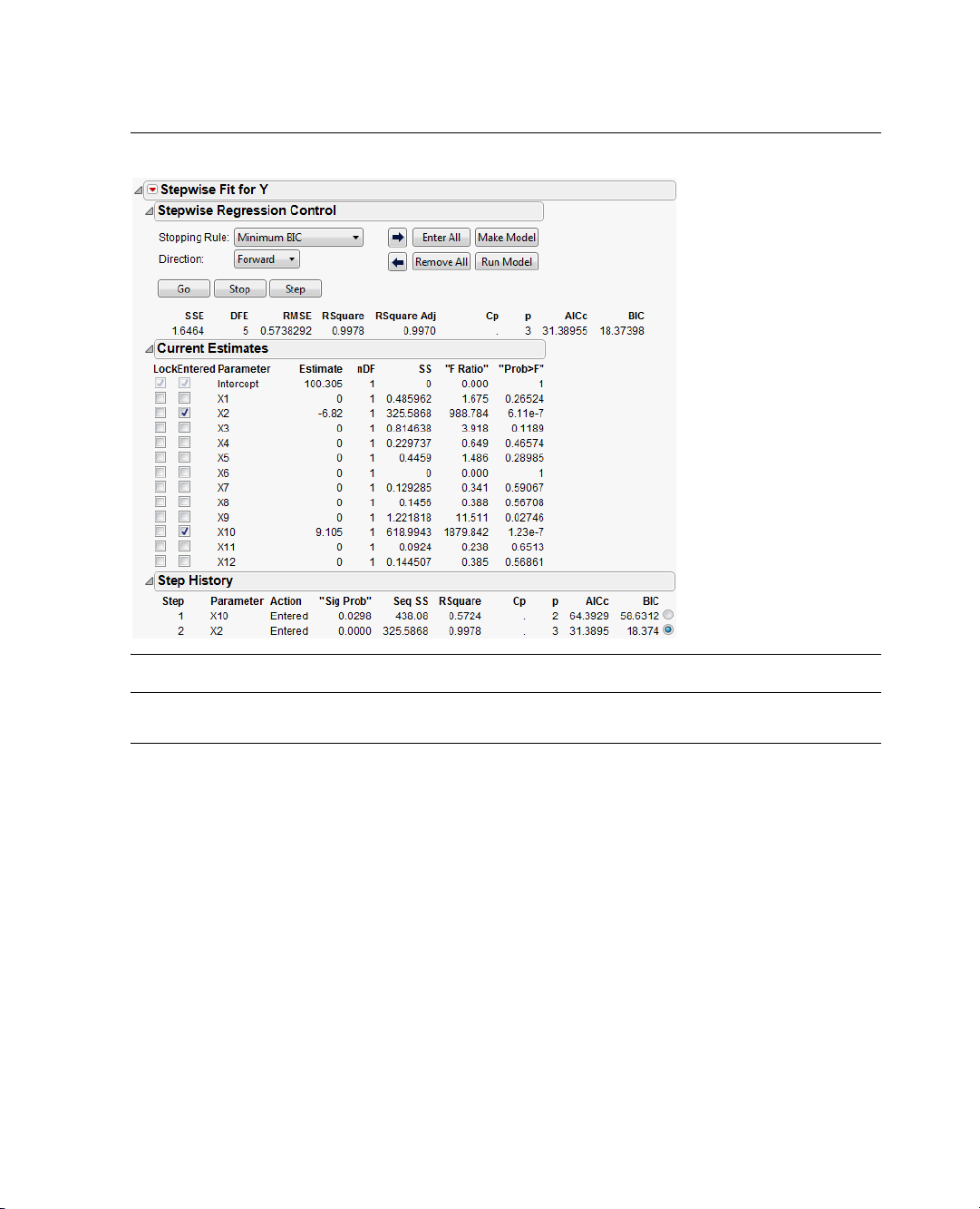
To identify active factors using stepwise regression:

1. To run the

2. Change the

Stepwise.

3. Click

4. In the resulting display click the

Model script in the design table, click the red triangle beside Model and select Run Script.

Personality in the Model Specification window from Standard Least Squares to

Run on the Fit Model dialog.

Step button two times. JMP enters the factors with the largest effects.

From the report that appears, you should identify two active factors, X2 and X10, as shown in Figure 2.11. The step history appears in the bottom part of the report. Because random noise is added, your estimates will be slightly different from those shown below.

26 Examples Using the Custom Designer Chapter 2

Creating Screening Experiments

Figure 2.11 Stepwise Regression Identifies Active Factors

Note: This example defines two large main effects and sets the rest to zero. In real-world situations, it may be less likely to have such clearly differentiated effects.

Screening Designs with Flexible Block Sizes

When you create a design using the Screening designer (DOE > Screening), the available block sizes for the listed designs are a power of two. However, custom designs in JMP can have blocks of any size. The blocking example shown in this section is flexible because it is using three runs per block, instead of a power of two.

After you select Values section of the Factors panel because the sample size is unknown at this point. After you complete the design, JMP shows the appropriate number of blocks, which is calculated as the sample size divided by the number of runs per block.

DOE > Custom Design and enter factors, the blocking factor shows only one level in the

Chapter 2 Examples Using the Custom Designer 27

Creating Screening Experiments

For example, Figure 2.12 shows that when you enter three continuous factors and one blocking factor with three runs per block, only one block appears in the Factors panel.

Figure 2.12 One Block Appears in the Factors Panel

The default sample size of nine requires three blocks. After you click Continue, there are three blocks in the Factors panel (Figure 2.13). This is because the default sample size is nine, which requires three blocks with three runs each.

Figure 2.13 Three Blocks in the Factors Panel

28 Examples Using the Custom Designer Chapter 2

Creating Screening Experiments

If you enter 24 runs in the User Specified box of the Number of Runs section, the Factors panel changes and now contains 8 blocks (Figure 2.14).

Figure 2.14 Number of Runs is 24 Gives Eight Blocks

If you add all the two-factor interactions and change the number of runs to 15, three runs per block produces five blocks (as shown in Figure 2.15), so the Factors panel displays five blocks in the Values section.

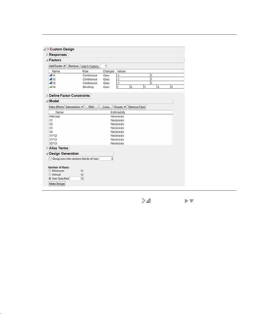
Chapter 2 Examples Using the Custom Designer 29

Creating Screening Experiments

Figure 2.15 Changing the Runs to 15

Click Make Design, then click the disclosure button ( on Windows and on the Macintosh) to open the

Design Evaluation outline node. Then, click the disclosure button to open the Relative Variance

of Coefficients report. Figure 2.16 shows the variance of each coefficient in the model relative to the unknown error variance.

The values in your table may be slightly different from those shown below. Notice that the variance of each coefficient is about one-tenth the error variance and that all the variances are roughly the same size. The error variance is assumed to be 1.

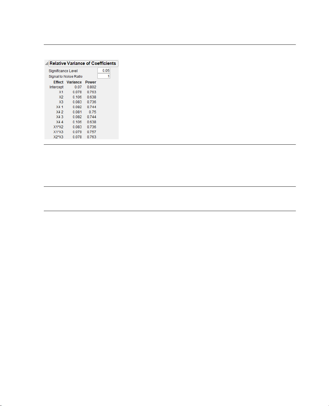
30 Examples Using the Custom Designer Chapter 2

Creating Screening Experiments

Figure 2.16 Table of Relative Variance of the Model Coefficients

The main question here is whether the relative size of the coefficient variance is acceptably small. If not, adding more runs (18 or more) will lower the variance of each coefficient.

For more details, see “The Relative Variance of Coefficients and Power Table,” p. 75.

Note to DOE experts: There are four rows associated with X4 (the block factor). That is because X4 has 5 blocks and, therefore, 4 degrees of freedom. Each degree of freedom is associated with one unknown coefficient in the model.

Checking for Curvature Using One Extra Run

In screening designs, experimenters often add center points and other check points to a design to help determine whether the assumed model is adequate. Although this is good practice, it is also ad hoc. The custom designer provides a way to improve on this ad hoc practice while supplying a theoretical foundation and an easy-to-use interface for choosing a design robust to the modeling assumptions.

The purpose of check points in a design is to provide a detection mechanism for higher-order effects that are contained in the assumed model. These higher-order terms are called potential terms. (Let q denote the potential terms, designated denote the primary terms designated

To take advantage of the benefits of the approach using larger than the number of

Possible

(potential) terms. That is, p < n < p+q. The formal name of the approach using If Possible model terms is Bayesian D-Optimal design. This type of design allows the precise estimation of all of the terms while providing omnibus detectability (and some estimability) for the

For a two-factor design having a model with an intercept, two main effects, and an interaction, there are p = 4 primary terms. When you enter this model in the custom designer, the default minimum runs value is a four-run design with the factor settings shown in Figure 2.17.

If Possible in JMP.) The assumed model consists of the primary terms. (Let p

Necessary in JMP.)

Necessary (primary) terms but smaller than the sum of the Necessary and If

If Possible model terms, the sample size should be

Necessary

If Possible terms.

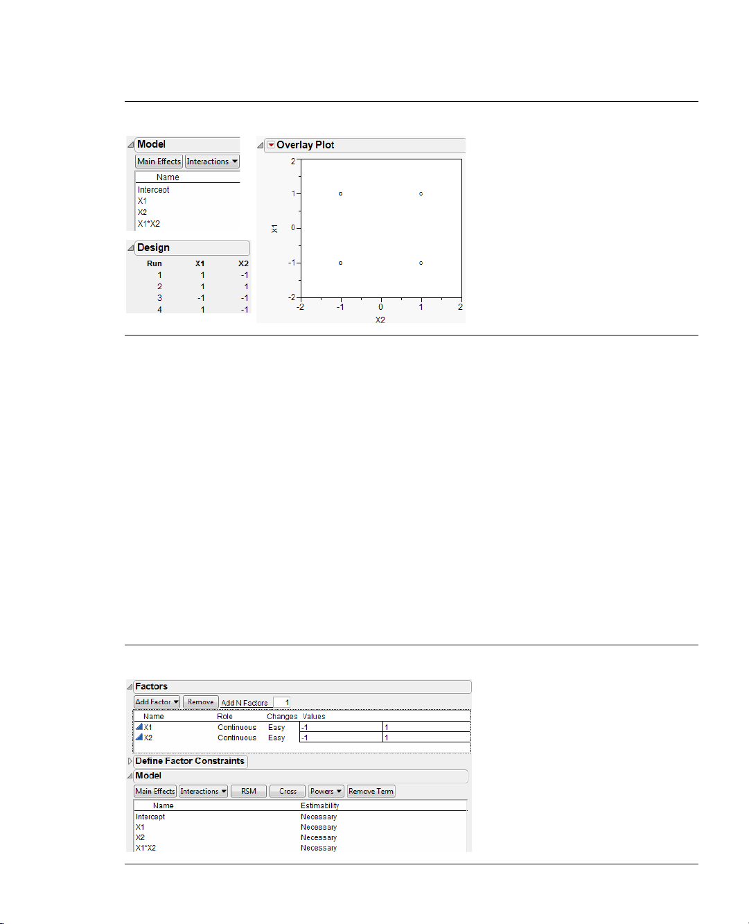
Chapter 2 Examples Using the Custom Designer 31

Creating Screening Experiments

Figure 2.17 Two Continuous Factors with Interaction

Now suppose you can afford an extra run (n = 5). You would like to use this point as a check point for curvature. If you leave the model the same and increase the sample size, the custom designer replicates one of the four vertices. Replicating any run is the optimal choice for improving the estimates of the terms in the model, but it provides no way to check for lack of fit.

Adding the two quadratic terms to the model makes a total of six terms. This is a way to model curvature directly. However, to do this the custom designer requires two additional runs (at a minimum), which exceeds your budget of five runs.

The Bayesian D-Optimal design provides a way to check for curvature while adding only one extra run. To create this design:

1. Select

2. Define two continuous factors (

3. Click

4. Choose

DOE > Custom Design.

X1 and X2).

Continue.

2nd from the Interactions menu in the Model panel. The results appear as shown in

Figure 2.18.

Figure 2.18 Second-Level Interactions

32 Examples Using the Custom Designer Chapter 2

Creating Screening Experiments

5. Choose 2nd from the Powers button in the Model panel. This adds two quadratic terms.

6. Select the two quadratic terms (

the menu and change

Figure 2.19 Changing the Estimability

Necessary to If Possible, as shown in Figure 2.19.

X1*X1 and X2*X2) and click the current estimability (Necessary) to see

Now, the p = 4 primary terms (the intercept, two main effects, and the interaction) are designated as

Necessary while the q = 2 potential terms (the two quadratic terms) are designated as If Possible. The

desired number of runs, five, is between p = 4 and p + q = 6.

7. Enter 5 into the User Specified edit box in the Number of Runs section of the Design Generation panel.

8. Click

Make Design. The resulting factor settings appear in Figure 2.20. The values in your design may

be different from those shown below.

Figure 2.20 Five-Run Bayesian D-Optimal Design

9. Click Make Table to create a JMP data table of the runs.

10. Create the overlay plot in Figure 2.21 with

Graph > Overlay Plot, and assign X1 as Y and X2 as X. The

overlay plot illustrates how the design incorporates the single extra run. In this example the design places the factor settings at the center of the design instead of at one of the corners.

Chapter 2 Examples Using the Custom Designer 33

Creating Response Surface Experiments

Figure 2.21 Overlay Plot of Five-run Bayesian D-Optimal Design

Creating Response Surface Experiments

Response surface experiments traditionally involve a small number (generally 2 to 8) of continuous factors. The a priori model for a response surface experiment is usually quadratic.

In contrast to screening experiments, researchers use response surface experiments when they already know which factors are important. The main goal of response surface experiments is to create a predictive model of the relationship between the factors and the response. Using this predictive model allows the experimenter to find better operating settings for the process.

In screening experiments one measure of the quality of the design is the size of the relative variance of the coefficients. In response surface experiments, the prediction variance over the range of the factors is more important than the variance of the coefficients. One way to visualize the prediction variance is JMP’s prediction variance profile plot. This plot is a powerful diagnostic tool for evaluating and comparing response surface designs.

Exploring the Prediction Variance Surface

The purpose of the example below is to generate and interpret a simple Prediction Variance Profile Plot. Follow the steps below to create a design for a quadratic model with a single continuous factor.

1. Select

2. Add one continuous factor by selecting

3. In the Model panel, select Powers > 2nd to create a quadratic term (Figure 2.22).

DOE > Custom Design.

Add Factor > Continuous (Figure 2.22), and click Continue.

34 Examples Using the Custom Designer Chapter 2

Creating Response Surface Experiments

Figure 2.22 Adding a Factor and a Quadratic Term

4. In the Design Generation panel, use the default number of runs (six) and click Make Design

(Figure 2.23). The number of runs is inversely proportional to the size of variance of the predicted response. As the number of runs increases, the prediction variances decrease.

Figure 2.23 Using the Default Number of Runs

5. Click the disclosure button ( on Windows and on the Macintosh) to open the Design

Evaluation

outline node, and then the Prediction Variance Profile, as shown in Figure 2.24.

For continuous factors, the initial setting is at the mid-range of the factor values. For categorical factors, the initial setting is the first level. If the design model is quadratic, then the prediction variance function is quartic. The y-axis is the relative variance of prediction of the expected value of the response.

In this design, the three design points are –1, 0, and 1. The prediction variance profile shows that the variance is a maximum at each of these points on the interval –1 to 1.

Figure 2.24 Prediction Profile for Single Factor Quadratic Model

Chapter 2 Examples Using the Custom Designer 35

Creating Response Surface Experiments

The prediction variance is relative to the error variance. When the relative prediction variance is one, the absolute variance is equal to the error variance of the regression model. More detail on the Prediction Variance Profiler is in “Understanding Design Evaluation,” p. 72.

6. To compare profile plots, click the

Back button and choose Minimum in the Design Generation panel,

which gives a sample size of three.

7. Click

Make Design and then open the Prediction Variance Profile again.

Now you see a curve that has the same shape as the previous plot, but the maxima are at one instead of 0.5. Figure 2.25 compares plots for a sample size of six and sample size of three for this quadratic model. You can see the prediction variance increase as the sample size decreases. Since the prediction variance is inversely proportional to the sample size, doubling the number of runs halves the prediction variance. These profiles show settings for the maximum variance and minimum variance, for sample sizes six (top charts) and sample size three (bottom charts). The axes on the bottom plots are adjusted to match the axes on the top plot.

Figure 2.25 Comparison of Prediction Variance Profiles

Tip: Click on the factor to set a factor level precisely.

8. To create an unbalanced design, click the text edit box in the Design Generation panel, then click

Back button and enter a sample size of 7 in the User Specified

Make Design. The results are shown in

Figure 2.26.

You can see that the variance of prediction at –1 is lower than the other sample points (its value is 0.33 instead of 0.5). The symmetry of the plot is related to the balance of the factor settings. When the design is balanced, the plot is symmetric, as shown in Figure 2.25. When the design is unbalanced, the prediction plot might not be symmetric, as shown in Figure 2.26.

36 Examples Using the Custom Designer Chapter 2

Prediction variance at X1= 0

Prediction variance at X1= –1

Creating Response Surface Experiments

Figure 2.26 Sample Size of Seven for the One-Factor Quadratic Model

Introducing I-Optimal Designs for Response Surface Modeling

The custom designer generates designs using a mathematical optimality criterion. All the designs in this chapter so far have been D-Optimal designs. D-Optimal designs are most appropriate for screening experiments because the optimality criterion focuses on precise estimates of the coefficients. If an experimenter has precise estimates of the factor effects, then it is easy to tell which factors’ effects are important and which are negligible. However, D-Optimal designs are not as appropriate for designing experiments where the primary goal is prediction.

I-Optimal designs minimize the average prediction variance inside the region of the factors. This makes I-Optimal designs more appropriate for prediction. As a result I-Optimality is the recommended criterion

for JMP response surface designs.

An I-Optimal design tends to place fewer runs at the extremes of the design space than does a D-Optimal design. As an example, consider a one-factor design for a quadratic model using n = 12 experimental runs. The D-Optimal design for this model puts four runs at each end of the range of interest and four runs in the middle. The I-Optimal design puts three runs at each end point and six runs in the middle. In this case, the D-Optimal design places two-thirds of its runs at the extremes versus one-half for the I-Optimal design.

Figure 2.27 compares prediction variance profiles of the one-factor I- and D-Optimal designs for a quadratic model with (n = 12) runs. The variance function for the I-Optimal design is less than the corresponding function for the D-Optimal design in the center of the design space; the converse is true at the edges.

Chapter 2 Examples Using the Custom Designer 37

Creating Response Surface Experiments

Figure 2.27 Prediction Variance Profiles for 12-Run I-Optimal (left) and D-Optimal (right) Designs

At the center of the design space, the average variance (relative to the error variance) for the I-Optimal design is 0.1667 compared to the D-Optimal design, which is 0.25. This means that confidence intervals for prediction will be nearly 10% shorter on average for the I-Optimal design.

To compare the two design criteria, create a one-factor design with a quadratic model that uses the I-Optimality criterion, and another one that uses D-Optimality:

1. Select

2. Add one continuous factor:

3. Click

4. Click the

DOE > Custom Design.

X1.

Continue.

RSM button in the Model panel to make the design I-Optimal.

5. Change the number of runs to 12.

6. Click

Make Design.

7. Click the disclosure button ( on Windows and on the Macintosh) to open the

Evaluation

outline node.

8. Click the disclosure button ( on Windows and on the Macintosh) to open the

Variance Profile

. (The Prediction Variance Profile is shown on the left in Figure 2.27.)

9. Repeat the same steps to create a D-Optimal design, but select

Design

from the red triangle menu on the custom design title bar. The results in the Prediction Variance

Profile should look the same as those on the right in Figure 2.27.

A Three-Factor Response Surface Design

In higher dimensions, the I-Optimal design continues to place more emphasis on the center of the region of the factors. The D-Optimal and I-Optimal designs for fitting a full quadratic model in three factors using 16 runs are shown in Figure 2.28.

To compare the two design criteria, create a three-factor design that uses the I-Optimality criterion, and another one that uses D-Optimality:

Design

Prediction

Optimality Criterion > Make D-Optimal

1. Select

DOE > Custom Design.

2. Add three continuous factors:

3. Click

Continue.

X1, X2, and X3.

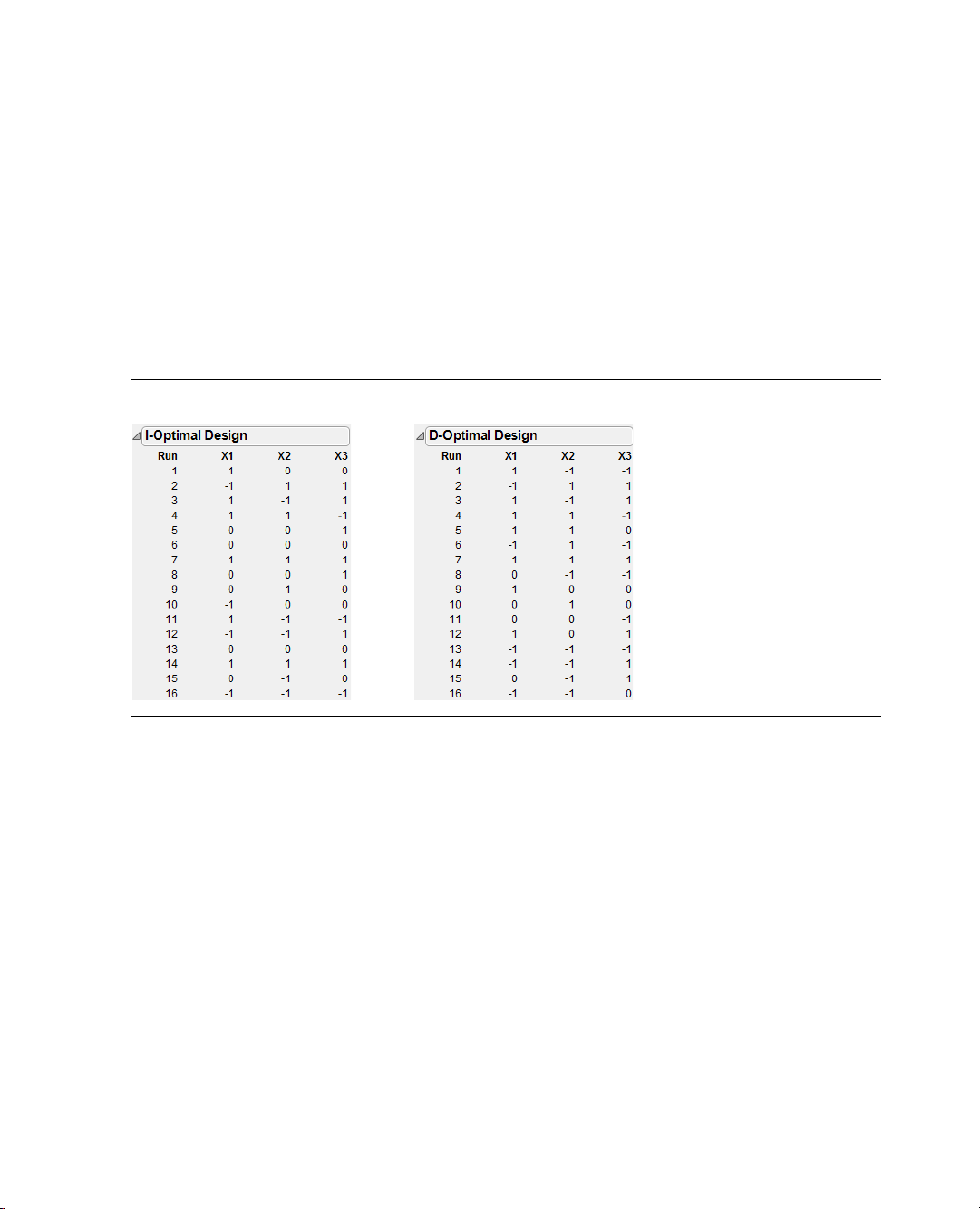
38 Examples Using the Custom Designer Chapter 2

Creating Response Surface Experiments

4. Click the RSM button in the Model panel to add interaction and quadratic terms to the model and to change the default optimality criterion to I-Optimal.

5. Use the default of 16 runs.

6. Click

Make Design.

The design is shown in the Design panel (the left in Figure 2.28).

7. If you want to create a D-Optimal design for comparison, repeat the same steps but select

Criterion > Make D-Optimal Design

from the red triangle menu on the custom design title bar. The

Optimality

design should look similar to those on the right in Figure 2.28. The values in your design may be different from those shown below.

Figure 2.28 16-run I-Optimal and D-Optimal designs for RSM Model

Profile plots of the variance function are displayed in Figure 2.29. These plots show slices of the variance function as a function of each factor, with all other factors fixed at zero. The I-Optimal design has the lowest prediction variance at the center. Note that there are two center points in this design.

The D-Optimal design has no center points and its prediction variance at the center of the factor space is almost three times the variance of the I-Optimal design. The variance at the vertices of the D-Optimal design is not shown. However, note that the D-Optimal design predicts better than the I-Optimal design near the vertices.

Chapter 2 Examples Using the Custom Designer 39

I-Optimal RSM Design with 16 runs

D-Optimal RSM Design with 16 runs

Creating Response Surface Experiments

Figure 2.29 Variance Profile Plots for 16 run I-Optimal and D-Optimal RSM Designs

Response Surface with a Blocking Factor

It is not unusual for a process to depend on both qualitative and quantitative factors. For example, in the chemical industry, the yield of a process might depend not only on the quantitative factors temperature and pressure, but also on such qualitative factors as the batch of raw material and the type of reactor. Likewise, an antibiotic might be given orally or by injection, a qualitative factor with two levels. The composition and dosage of the antibiotic could be quantitative factors (Atkinson and Donev, 1992).

The response surface designer (described in “Response Surface Designs,” p. 127) only deals with quantitative factors. You could use the response surface designer to produce a Response Surface Model (RSM) design with a qualitative factor by replicating the design over each level of the factor. But, this is unnecessarily time-consuming and expensive. Using custom designer is simpler and more cost-effective because fewer runs are required. The following steps show how to accommodate a blocking factor in a response surface design using the custom designer:

1. First, define two continuous factors (

2. Now, click

Add Factor and select Blocking > 4 runs per block to create a blocking factor(X3). The

blocking factor appears with one level, as shown in Figure 2.30, but the number of levels adjusts later to accommodate the number of runs specified for the design.

X1 and X2).

40 Examples Using the Custom Designer Chapter 2

Creating Response Surface Experiments

Figure 2.30 Add Two Continuous Factors and a Blocking Factor

3. Click Continue, and then click RSM in the Model panel to add the quadratic terms to the model (Figure 2.31). This automatically changes the recommended optimality criterion from D-Optimal to I-Optimal. Note that when you click RSM, a message reminds you that nominal factors (such as the blocking factor) cannot have quadratic effects.

Figure 2.31 Add Response Surface Terms

4. Enter 12 in the User Specified text edit box in the Design Generation panel, and note that the Factors panel now shows the Blocking factor,

X3, with three levels (Figure 2.32). Twelve runs defines three

blocks with four runs per block.

Chapter 2 Examples Using the Custom Designer 41

Creating Response Surface Experiments

Figure 2.32 Blocking Factor Now Shows Three Levels

5. Click Make Design.

6. In the Output Options, select

7. Click

Make Table to see an I-Optimal table similar to the one on the left in Figure 2.33.

Sort Right to Left from the Run Order list.

Figure 2.33 compares the results of a 12-run I-Optimal design and a 12-run D-Optimal Design.

To see the D-Optimal design:

1. Click the

2. Click the red triangle icon on the Custom Design title bar and select

D-Optimal Design

Back button.

Optimality Criterion > Make

3. Click Make Design, then click Make Table.

Figure 2.33 JMP Design Tables for 12-Run I-Optimal and D-Optimal Designs

42 Examples Using the Custom Designer Chapter 2

Creating Response Surface Experiments

Figure 2.34 gives a graphical view of the designs generated by this example. These plots were generated for the runs in each JMP table by choosing factor (

X3) as the Grouping variable.

Graph > Overlay Plot from the main menu andusing the blocking

Note that there is a center point in each block of the I-Optimal design. The D-Optimal design has only one center point. The values in your graph may be different from those shown in Figure 2.34.

Figure 2.34 Plots of I-Optimal (left) and D-Optimal (right) Design Points by Block.

Either of the designs in Figure 2.34 supports fitting the specified model. The D-Optimal design does a slightly better job of estimating the model coefficients. The diagnostics (Figure 2.35) for the designs show beneath the design tables. In this example, the D-efficiency of the I-Optimal design is about 51%, and is 55% for the D-Optimal design.

The I-Optimal design is preferable for predicting the response inside the design region. Using the formulas given in “Technical Discussion,” p. 59, you can compute the relative average variance for these designs. The average variance (relative to the error variance) for the I-Optimal design is 0.5 compared to 0.59 for the D-Optimal design (See Figure 2.35). This means confidence intervals for prediction will be almost 20% longer on average for D-Optimal designs.

Chapter 2 Examples Using the Custom Designer 43

Creating Mixture Experiments

Figure 2.35 Design Diagnostics for I-Optimal and D-Optimal Designs

Creating Mixture Experiments

If you have factors that are ingredients in a mixture, you can use either the custom designer or the specialized mixture designer. However, the mixture designer is limited because it requires all factors to be mixture components and you might want to vary the process settings along with the percentages of the mixture ingredients. The optimal formulation could change depending on the operating environment. The custom designer can handle mixture ingredients and process variables in the same study. You are not forced to modify your problem to conform to the restrictions of a special-purpose design approach.

Mixtures Having Nonmixture Factors

The following example from Atkinson and Donev (1992) shows how to create designs for experiments with mixtures where one or more factors are not ingredients in the mixture. In this example:

• The response is the electromagnetic damping of an acrylonitrile powder.

• The three mixture ingredients are copper sulphate, sodium thiosulphate, and glyoxal.

• The nonmixture environmental factor of interest is the wavelength of light.

Though

wavelength is a continuous variable, the researchers were only interested in predictions at three

discrete wavelengths. As a result, they treated it as a categorical factor with three levels. To create this custom design:

1. Select

2. Create

3. In the Factors panel, add the three mixture ingredients and the categorical factor,

DOE > Custom Design.

Damping as the response. The authors do not mention how much damping is desirable, so

right-click the goal and create

Damping’s response goal to be None.

Wavelength. The

mixture ingredients have range constraints that arise from the mechanism of the chemical reaction. Rather than entering them by hand, load them from the Sample Data folder that was installed with JMP: click the red triangle icon on the Custom Design title bar and select

Mixture Factors.jmp

, from the Design Experiment sample data folder. The custom design panels should

Load Factors. Open Donev

now look like those shown in Figure 2.36.

44 Examples Using the Custom Designer Chapter 2

Creating Mixture Experiments

Figure 2.36 Mixture Experiment Response Panel and Factors Panel

The model, shown in Figure 2.37 is a response surface model in the mixture ingredients along with the additive effect of the wavelength. To create this model:

1. Click

Interactions, and choose 2nd. A warning dialog appears telling you that JMP removes the main

effect terms for non-mixture factors that interact with all the mixture factors. Click

2. In the Design Generation panel, type 18 in the

User Specified text edit box (Figure 2.37), which results

in six runs each for the three levels of the wavelength factor.

OK.

Chapter 2 Examples Using the Custom Designer 45

Creating Mixture Experiments

Figure 2.37 Mixture Experiment Design Generation Panel

3. Click Make Design, and then click Make Table.

The resulting data table is shown in Figure 2.38. The values in your table may be different from those shown below.

46 Examples Using the Custom Designer Chapter 2

Creating Mixture Experiments

Figure 2.38 Mixture Experiment Design Table

Atkinson and Donev also discuss the design where the number of runs is limited to 10. In that case, it is not possible to run a complete mixture response surface design for every wavelength.

To v i e w t h is :

1. Click the

2. Remove all the effects by highlighting them and clicking

3. Add the main effects by clicking the

Back button.

Remove Term.

Main Effects button.

4. In the Design Generation panel, change the number of runs to 10 (Figure 2.39) and click

Design

. The Design table to the right in Figure 2.39 shows the factor settings for 10 runs.

Figure 2.39 Ten-Run Mixture Response Surface Design

Make

Chapter 2 Examples Using the Custom Designer 47

Creating Mixture Experiments

Note that there are necessarily unequal numbers of runs for each wavelength. Because of this lack of balance it is a good idea to look at the prediction variance plot (top plot in Figure 2.40).

5. Open the

Design Evaluation outline node, then open the Prediction Variance Profile.

The prediction variance is almost constant across the three wavelengths, which is a good indication that the lack of balance is not a problem.

The values of the first three ingredients sum to one because they are mixture ingredients. If you vary one of the values, the others adjust to keep the sum constant.

6. Select

Maximize Desirability from red triangle menu on the Prediction Variance Profile title bar, as

shown in the bottom profiler in Figure 2.40.

The most desirable wavelength is percentage is zero, and

Figure 2.40 Prediction Variance Plots for Ten-Run Design

Na2S2O3 is 0.8, which maintains the mixture.

L3, with the CuSO4 percentage decreasing from about 0.4 to 0.2, Glyoxal

Experiments that are Mixtures of Mixtures

As a way to illustrate the idea of a ‘mixture of mixtures’ situation, imagine the ingredients that go into baking a cake and assume the following:

• dry ingredients composed of flour, sugar, and cocoa

• wet (or non-dry) ingredients consisting of milk, melted butter, and eggs.

These two components (wet and dry) of the cake are two mixtures that are first mixed separately and then blended together.

48 Examples Using the Custom Designer Chapter 2

Creating Mixture Experiments

The dessert chef knows that the dry component (the mixture of flour, sugar, and cocoa) contributes 45% of the combined mixture and the wet component (butter, milk, and eggs) contributes 55%.

The objective of such an experiment might be to identify proportions within the two components that maximize some measure of taste or consistency.

This is a main effects model except that you must leave out one of the factors in order to avoid singularity. The choice of which factor to leave out of the model is arbitrary.

For now, consider these upper and lower levels of the various factors:

Within the dry mixture:

• cocoa must be greater than 10% but less than 20%

• sugar must be greater than 0% but less than 15%

• flour must be greater than 20% but less than 30%

Within the wet mixture:

• melted butter must be greater than 10% but less than 20%

• milk must be greater than 25% and less than 35%

• eggs constitute more than 5% but less than 20%

You want to bake cakes and measure taste on a scale from 1 to 10

Use the Custom Designer to set up this example, as follows:

1. In the Response Panel, enter one response and call it

2. Give Taste a

Lower Limit of 1 and an Upper Limit of 10. (You are assuming a taste test where the

Ta st e .

respondents reply on a scale of 1 to 10.)

3. In the Factors Panel, enter the six cake factors described above.

4. Enter the given percentage values of the factors as proportions in the

Values section of the Factors panel.

The completed Response and Factors panels should look like those shown in Figure 2.41.

Chapter 2 Examples Using the Custom Designer 49

Creating Mixture Experiments

Figure 2.41 Completed Responses and Factors Panel for the Cake Example

5. Next, click Continue.

6. Open the Define Factor Constraints pane and click Add Constraint twice.

7. Enter the constraints as shown in Figure 2.42. For the second constraint setting, click on the less than or equal to button and select the greater than or equal to direction.

By confining the dry factors to exactly 45% in this way, the mixture role of all the factors ensures that the wet factors constitute the remaining 55%.

8. Open the Model dialog and note that it lists all 6 effects. Because these are mixture factors, including all effects would render the model singular. Highlight any one of the terms in the model and click

Te rm

, as shown.

Figure 2.42 Constraints to Define the Double Mixture Experiment

Remove

50 Examples Using the Custom Designer Chapter 2

Each run sums to 0.55 (55%)

Each run sums to 0.45 (45%)

Special-Purpose Uses of the Custom Designer

9. To see a completed example, choose Simulate Responses from the menu on the Custom Design title bar.

10. In the Design Generation panel, enter 10 as the number of runs for the example. That is, you would bake cakes with 10 different sets of ingredient proportions.

11. Click

The table inFigure 2.43 shows that the two sets of cake ingredients (dry and wet) adhere to the proportions 45% and 55% as defined by the entered constraints. In addition, the amount of each ingredient in each cake recipe (run) conforms to the upper and lower limits given in the factors dialog.

Figure 2.43 Cake Experiment Conforming to a Mixture of Mixture Design

Make Design in the Design Generation panel, and then click Make Table.

Note: As a word of caution, keep in mind that it is easy to define constraints in such a way that it is impossible to construct a design that fits the model. In such a case, you will get a message saying “Could not find a valid starting design. Please check your constraints for consistency.”

Special-Purpose Uses of the Custom Designer

While some of the designs discussed in previous sections can be created using other designers in JMP or by looking them up in a textbook containing tables of designs, the designs presented in this section cannot be created without using the custom designer.

Designing Experiments with Fixed Covariate Factors

Pre-tabulated designs rely on the assumption that the experimenter controls all the factors. Sometimes you have quantitative measurements (a covariate) on the experimental units before the experiment begins. If this variable affects the experimental response, the covariate should be a design factor. The pre-defined design that allows only a few discrete values is too restrictive. The custom designer supplies a reasonable design option.

Chapter 2 Examples Using the Custom Designer 51

Special-Purpose Uses of the Custom Designer

For this example, suppose there are a group of students participating in a study. A physical education researcher has proposed an experiment where you vary the number of hours of sleep and the calories for breakfast and ask each student to run 1/4 mile. The weight of the student is known and it seems important to include this information in the experimental design.

To follow along with this example that shows column properties, open

Big Class.jmp from the Sample Data

folder that was installed when you installed JMP.

Build the custom design as follows:

1. Select

DOE > Custom Design.

2. Add two continuous variables to the models by entering 2 beside Add N Factors, clicking and selecting

3. Click

Continuous, naming them calories and sleep.

Add Factor and select Covariate, as shown in Figure 2.44. The Covariate selection displays a list

of the variables in the current data table.

Figure 2.44 Add a Covariate Factor

4. Select weight from the variable list (Figure 2.45) and click OK.

Add Factor

Figure 2.45 Design with Fixed Covariate

5. Click Continue.

6. Add the interaction to the model by selecting panel, and then clicking the

Cross button (Figure 2.46).

calories in the Factors panel, selecting sleep in the Model

52 Examples Using the Custom Designer Chapter 2

Special-Purpose Uses of the Custom Designer

Figure 2.46 Design With Fixed Covariate Factor

7. Click Make Design, then click Make Table. The data table in Figure 2.47 shows the design table. Your runs might not look the same because the order of the runs has been randomized.

Figure 2.47 Design Table for Covariate Example

Note: Covariate factors cannot have missing values.

Remember that custom designer has calculated settings for correlations between designer did by fitting a model of

weight is the covariate factor, measured for each student, but it is not controlled. The

calories and sleep for each student. It would be desirable if the

calories, sleep and weight were as small as possible. You can see how well the custom

weight as a function of calories and sleep. If that fit has a small model

sum of squares, that means the custom designer has successfully separated the effect of weight from the effects of calories and sleep.

Chapter 2 Examples Using the Custom Designer 53

Special-Purpose Uses of the Custom Designer

8. Click the red triangle icon beside Model in the data table and select Run Script, as shown on the left in Figure 2.48.

Figure 2.48 Model Script

9. Rearrange the dialog so weight is Y and calories, sleep, and calories*sleep are the model effects, as shown to the right in Figure 2.48. Click

Run.

The leverage plots are nearly horizontal, and the analysis of variance table shows that the model sum of squares is near zero compared to the residuals (Figure 2.49). Therefore, and

sleep. The values in your analysis may be a little different from those shown below.

weight is independent of calories

Figure 2.49 Analysis to Check That Weight is Independent of Calories and Sleep

54 Examples Using the Custom Designer Chapter 2

Special-Purpose Uses of the Custom Designer

Creating a Design with Two Hard-to-Change Factors: Split Plot

While there is substantial research literature covering the analysis of split plot designs, it has only been possible in the last few years to create optimal split plot designs (Goos 2002). The split plot design capability accessible in the JMP custom designer is the first commercially available tool for generating optimal split plot designs.

The split plot design originated in agriculture, but is commonplace in manufacturing and engineering studies. In split plot experiments, hard-to-change factors only change between one whole plot and the next. The whole plot is divided into subplots, and the levels of the easy-to-change factors are randomly assigned to each subplot.

The example in this section is adapted from Kowalski, Cornell, and Vining (2002). The experiment studies the effect of five factors on the thickness of vinyl used to make automobile seat covers. The response and factors in the experiment are described below:

• Three of the factors are ingredients in a mixture. They are plasticizers whose proportions,

m3, sum to one. Additionally, the mixture components are the subplot factors of the experiment.

• Two of the factors are process variables. They are the rate of extrusion ( temperature (

temperature) of drying. These process variables are the whole plot factors of the

extrusion rate) and the

m1, m2, and

experiment. They are hard to change.

• The response in the experiment is the thickness of the vinyl used for automobile seat covers. The response of interest (

thickness) depends both on the proportions of the mixtures and on the effects of

the process variables.

To create this design in JMP:

1. Select

2. By default, there is one response,

DOE > Custom Design.

default goal,

Maximize (Figure 2.50).

Y, showing. Double-click the name and change it to thickness. Use the

3. Enter the lower limit of 10.

4. To add three mixture factors, type 3 in the box beside

Add N Factors, and click Add Factor > Mixture.

5. Name the three mixture factors m1, m2, and m3. Use the default levels 0 and 1 for those three factors.

6. Add two continuous factors by typing 2 in the box beside

Continuous

. Name these factors extrusion rate and temperature.

Add N Factors, and click Add Factor >

7. Ensure that you are using the default levels, –1 and 1, in the Values area corresponding to these two factors.

8. To make

9. To make

extrusion rate a whole plot factor, click Easy and select Hard.

temperature a whole plot factor, click Easy and select Hard. Your dialog should look like the

one in Figure 2.50.

Chapter 2 Examples Using the Custom Designer 55

Special-Purpose Uses of the Custom Designer

Figure 2.50 Entering Responses and Factors

10. Click Continue.

11. Next, add interaction terms to the model by selecting

Interactions > 2nd (Figure 2.51). This causes a

warning that JMP removes the main effect terms for non-mixture factors that interact with all the mixture factors. Click

OK.

Figure 2.51 Adding Interaction Terms

12. In the Design Generation panel, type 7 in the Number of Whole Plots text edit box.

13. For

Number of Runs, type 28 in the User Specified text edit box (Figure 2.52).

56 Examples Using the Custom Designer Chapter 2

X′V1–X

Special-Purpose Uses of the Custom Designer

Figure 2.52 Assigning the Number of Whole Plots and Number of Runs

Note: If you enter a missing value in the Number of Whole Plots edit box, then JMP considers many

different numbers of whole plots and chooses the number that maximizes the information about the coefficients in the model. It maximizes the determinant of where V

is the inverse of the variance matrix of the responses. The matrix, V, is a function of how many whole plots there are, so changing the number of whole plots changes V, which can make a difference in the amount of information a design contains.

14. Click

Figure 2.53 Partial Listing of the Final Design Structure

Make Design. The result is shown in Figure 2.53.

15. Click Make Table.

16. From the Sample Data folder that was installed with JMP, open

Experiment

folder, which contains 28 runs as well as response values. The values in the table you

Vinyl Data.jmp from the Design

generated with the custom designer may be different from those from the Sample Data folder, shown in Figure 2.54.

Chapter 2 Examples Using the Custom Designer 57

Special-Purpose Uses of the Custom Designer

Figure 2.54 The Vinyl Data Design Table

17. Click the red triangle icon next to the Model script and select Run Script. The dialog in Figure 2.55 appears.

The models for split plots have a random effect associated with the whole plots’ effect.

As shown in the dialog in Figure 2.55, JMP designates the error term by appending &Random to the name of the effect. REML will be used for the analysis, as indicated in the menu beside

Method in Figure 2.55.

For more information about REML models, see Modeling and Multivariate Methods.

58 Examples Using the Custom Designer Chapter 2

Special-Purpose Uses of the Custom Designer

Figure 2.55 Define the Model in the Fit Model Dialog

18. Click Run to run the analysis. The results are shown in Figure 2.56.

Chapter 2 Examples Using the Custom Designer 59

Technical Discussion

Figure 2.56 Split Plot Analysis Results

Technical Discussion

This section provides information about I-, D-, Bayesian I-, Bayesian D-, and Alias-Optimal designs.

D-Optimality:

• is the default design type produced by the custom designer except when the RSM button has been clicked to create a full quadratic model.

• minimizes the variance of the model coefficient estimates. This is appropriate for first-order models and in screening situations, because the experimental goal in such situations is often to identify the active factors; parameter estimation is key.

• is dependent on a pre-stated model. This is a limitation because in most real situations, the form of the pre-stated model is not known in advance.

• has runs whose purpose is to lower the variability of the coefficients of this pre-stated model. By focusing on minimizing the standard errors of coefficients, a D-Optimal design may not allow for checking that the model is correct. It will not include center points when investigating a first-order model. In the extreme, a D-Optimal design may have just p distinct runs with no degrees of freedom for lack of fit.

60 Examples Using the Custom Designer Chapter 2

D det X′X[]=

D det X′V1–X[]=



′ x()X′X()=

1–

fx()dx

Trace X′X()1–M[]=

Technical Discussion

• maximizes D when

D-optimal split plot designs maximize D when

-1

where V

is the block diagonal variance matrix of the responses (Goos 2002).

Bayesian D-Optimality:

• is a modification of the D-Optimality criterion that effectively estimates the coefficients in a model, and at the same time has the ability to detect and estimate some higher-order terms. If there are interactions or curvature, the Bayesian D-Optimality criterion is advantageous.

• works best when the sample size is larger than the number of of the

Necessary and If Possible terms. That is, p + q > n > p. The Bayesian D-Optimal design is an

approach that allows the precise estimation of all of the detectability (and some estimability) for the

• uses the containing only the

If Possible terms to force in runs that allow for detecting any inadequacy in the model

Necessary terms. Let K be the (p + q) by (p + q) diagonal matrix whose first p

If Possible terms.

Necessary terms but smaller than the sum

Necessary terms while providing omnibus

diagonal elements are equal to 0 and whose last q diagonal elements are the constant, k. If there are 2-factor interactions then k = 4. Otherwise k = 1. The Bayesian D-Optimal design maximizes the determinant of (X'X + K). The difference between the criterion for D-Optimality and Bayesian D-Optimality is this constant added to the diagonal elements corresponding to the

If Possible terms in

the X'X matrix.

I-Optimality:

• minimizes the average variance of prediction over the region of the data.

• is more appropriate than D-Optimality if your goal is to predict the response rather than the coefficients, such as in response surface design problems. Using the I-Optimality criterion is more appropriate because you can predict the response anywhere inside the region of data and therefore find the factor settings that produce the most desirable response value. It is more appropriate when your objective is to determine optimum operating conditions, and also is appropriate to determine regions in the design space where the response falls within an acceptable range. Precise estimation of the response therefore takes precedence over precise estimation of the parameters.

• maximizes this criterion: If f '(x) denotes a row of the X matrix corresponding to factor combinations x, then

where

Chapter 2 Examples Using the Custom Designer 61

M f



x()fx()′dx=

var





x0′

X′XK+





1–





Trace X′XK+()

1–

M[]=

X1′X

()1–X1′X

tr AA'()

AA'

Technical Discussion

is a moment matrix that is independent of the design and can be computed in advance.

Bayesian I-Optimality:

Bayesian I-Optimality has a different objective function to optimize than the Bayesian D-optimal design, so the designs that result are different. The variance matrix of the coefficients for Bayesian I-optimality is X'X + K where K is a matrix having zeros for the

If Possible model terms.

Necessary model terms and some constant value for the

The variance of the predicted value at a point x

is:

The Bayesian I-Optimal design minimizes the average prediction variance over the design region:

where M is defined as before.

Alias Optimality:

• seeks to minimize the aliasing between model effects and alias effects.

Specifically, let X

be the design matrix corresponding to the model effects, and let X2 be the matrix of alias

effects, and let

A =

be the alias matrix.

Then, alias optimality seeks to minimize the , subject to the D-Efficiency being greater than some lower bound. In other words, it seeks to minimize the sum of the squared diagonal elements of .

62 Examples Using the Custom Designer Chapter 2

Technical Discussion

Chapter 3

Building Custom Designs

The Basic Steps

JMP can build a custom design that both matches the description of your engineering problem and remains within your budget for time and material. Custom designs are general, flexible, and good for routine factor screening or response optimization. To create these tailor-made designs, use the found on the

This chapter introduces you to the steps you need to complete to build a custom design.

DOE menu or the Custom Design button found on the DOE panel of the JMP Starter.

Custom Design command

Contents

Creating a Custom Design . . . . . . . . . . . . . . . . . . . . . . . . . . . . . . . . . . . . . . . . . . . . . . . . . . . . . . . . . . . .65

Enter Responses and Factors into the Custom Designer . . . . . . . . . . . . . . . . . . . . . . . . . . . . . . . . . . .65

Describe the Model . . . . . . . . . . . . . . . . . . . . . . . . . . . . . . . . . . . . . . . . . . . . . . . . . . . . . . . . . . . . . . 69

Specifying Alias Terms. . . . . . . . . . . . . . . . . . . . . . . . . . . . . . . . . . . . . . . . . . . . . . . . . . . . . . . . . . . . 70

Select the Number of Runs . . . . . . . . . . . . . . . . . . . . . . . . . . . . . . . . . . . . . . . . . . . . . . . . . . . . . . . . .71

Understanding Design Evaluation . . . . . . . . . . . . . . . . . . . . . . . . . . . . . . . . . . . . . . . . . . . . . . . . . . . 72

Specify Output Options . . . . . . . . . . . . . . . . . . . . . . . . . . . . . . . . . . . . . . . . . . . . . . . . . . . . . . . . . . 78

Make the JMP Design Table . . . . . . . . . . . . . . . . . . . . . . . . . . . . . . . . . . . . . . . . . . . . . . . . . . . . . . . 79

Creating Random Block Designs. . . . . . . . . . . . . . . . . . . . . . . . . . . . . . . . . . . . . . . . . . . . . . . . . . . . . . . 80

Creating Split Plot Designs . . . . . . . . . . . . . . . . . . . . . . . . . . . . . . . . . . . . . . . . . . . . . . . . . . . . . . . . . . . 80

Creating Split-Split Plot Designs . . . . . . . . . . . . . . . . . . . . . . . . . . . . . . . . . . . . . . . . . . . . . . . . . . . . . . . .81

Creating Strip Plot Designs . . . . . . . . . . . . . . . . . . . . . . . . . . . . . . . . . . . . . . . . . . . . . . . . . . . . . . . . . . . .82

Special Custom Design Commands. . . . . . . . . . . . . . . . . . . . . . . . . . . . . . . . . . . . . . . . . . . . . . . . . . . . . .83

Save Responses and Save Factors . . . . . . . . . . . . . . . . . . . . . . . . . . . . . . . . . . . . . . . . . . . . . . . . . . . . 84

Load Responses and Load Factors . . . . . . . . . . . . . . . . . . . . . . . . . . . . . . . . . . . . . . . . . . . . . . . . . . . .85

Save Constraints and Load Constraints . . . . . . . . . . . . . . . . . . . . . . . . . . . . . . . . . . . . . . . . . . . . . . . .85

Set Random Seed: Setting the Number Generator. . . . . . . . . . . . . . . . . . . . . . . . . . . . . . . . . . . . . . . .85

Simulate Responses . . . . . . . . . . . . . . . . . . . . . . . . . . . . . . . . . . . . . . . . . . . . . . . . . . . . . . . . . . . . . . 86

Save X Matrix: Viewing the Number of Rows in the Moments Matrix and the Design Matrix (X) in the

Log . . . . . . . . . . . . . . . . . . . . . . . . . . . . . . . . . . . . . . . . . . . . . . . . . . . . . . . . . . . . . . . . . . . . . . . 87

Optimality Criterion . . . . . . . . . . . . . . . . . . . . . . . . . . . . . . . . . . . . . . . . . . . . . . . . . . . . . . . . . . . . . .88

Number of Starts: Changing the Number of Random Starts . . . . . . . . . . . . . . . . . . . . . . . . . . . . . . . .88

Sphere Radius: Constraining a Design to a Hypersphere . . . . . . . . . . . . . . . . . . . . . . . . . . . . . . . . . . 90

Disallowed Combinations: Accounting for Factor Level Restrictions. . . . . . . . . . . . . . . . . . . . . . . . . 90

Advanced Options for the Custom Designer . . . . . . . . . . . . . . . . . . . . . . . . . . . . . . . . . . . . . . . . . . . 92

Assigning Column Properties . . . . . . . . . . . . . . . . . . . . . . . . . . . . . . . . . . . . . . . . . . . . . . . . . . . . . . . . . .93

Define Low and High Values (DOE Coding) for Columns . . . . . . . . . . . . . . . . . . . . . . . . . . . . . . . . 94

Set Columns as Factors for Mixture Experiments . . . . . . . . . . . . . . . . . . . . . . . . . . . . . . . . . . . . . . . .95

Define Response Column Values . . . . . . . . . . . . . . . . . . . . . . . . . . . . . . . . . . . . . . . . . . . . . . . . . . . . 96

Assign Columns a Design Role . . . . . . . . . . . . . . . . . . . . . . . . . . . . . . . . . . . . . . . . . . . . . . . . . . . . . 97

Identify Factor Changes Column Property . . . . . . . . . . . . . . . . . . . . . . . . . . . . . . . . . . . . . . . . . . . . 98

How Custom Designs Work: Behind the Scenes . . . . . . . . . . . . . . . . . . . . . . . . . . . . . . . . . . . . . . . . . . . 99

Chapter 3 Building Custom Designs 65

Creating a Custom Design

To begin, select DOE > Custom Design, or click the Custom Design button on the JMP Starter DOE page. Then, follow the steps below.

• Enter responses and factors into the custom designer.

• Describe the model.

• Select the number of runs.

• Check the design diagnostics, if desired.

• Specify output options.

• Make the JMP design table.

The following sections describe each of these steps.

Enter Responses and Factors into the Custom Designer

How to Enter Responses

To enter responses, follow the steps in Figure 3.1.

1. To enter one response at a time, click Add Response, and then select a goal type. Possible goal types are

Maximize, Match Target, Minimize, or None.

2. (Optional) Double-click to edit the response name.

3. (Optional) Click to change the response goal.

4. Click to enter lower and upper limits and importance weights.

Figure 3.1 Entering Responses

Tip: To quickly enter multiple responses, click Number of Responses and enter the number of responses you want.

66 Building Custom Designs Chapter 3

Creating a Custom Design

Specifying Response Goal Types and Lower and Upper Limits

When entering responses, you can tell JMP that your goal is to obtain the maximum or minimum value possible, to match a specific value, or that there is no response goal.

The following description explains the relationship between the goal type (step 3 in Figure 3.1) and the lower and upper limits (step 4 in Figure 3.1):

• For responses such as strength or yield, the best value is usually the largest possible. A goal of supports this objective.

•The

Minimize goal supports an objective of having the smallest value, such as when the response is

impurity or defects.

•The

Match Target goal supports the objective when the best value for a response is a specific target

value, such as a dimension for a manufactured part. The default target value is assumed to be midway between the given lower and upper limits.

Note: If your target response is not equidistant from the lower and upper acceptable bounds, you can alter the default target after you make a table from the design. In the data table, open the Column Info dialog for the response column (Cols > Column Info) and enter the desired target value.

Understanding Response Importance Weights

To compute and maximize overall desirability, JMP uses the value you enter as the importance weight (step 4 in Figure 3.1) of each response. If there is only one response, then importance weight is unnecessary. With two responses you can give greater weight to one response by assigning it a higher importance value.

Adding Simulated Responses, If Desired

If you do not have values for specific responses, you might want to add simulated responses to see a prospective analysis in advance of real data collection.

1. Create the design.

2. Before you click

3. Click

Make Table to create the design table. The Y column contains values for simulated responses.

Make Table, click the red triangle icon in the title bar and select Simulate Responses.

4. For custom and augment designs, a window (Figure 3.2) appears along with the design data table. In this window, enter values you want to apply to the numbers you enter represent the coefficients in an equation. An example of such an equation, as shown in Figure 3.2, would be, y =28+4X1+5X2+random noise, where the random noise is distributed with mean zero and standard deviation one.

Maximize

Y column in the data table and click Apply. The

Chapter 3 Building Custom Designs 67

Creating a Custom Design

Figure 3.2 In Custom and Augment Designs, Specify Values for Simulated Responses

How to Enter Factors

To enter factors, follow the steps in Figure 3.3.

1. To add one factor, click

Categorical, Blocking, Covariate, Mixture, Constant, or Uncontrolled. See “Types of Factors,” p. 67.

2. Click a factor and select

Add Factor and select a factor type. Possible factor types are Continuous,

Add Level to increase the number of levels.

3. Double-click a factor to edit the factor name.

4. Click to indicate that changing a factor’s setting from run to run is

Easy or Hard. Changing to Hard

will cause the resulting design to be a split plot design.

5. Click to enter or change factor values. To remove a level, click it, press the delete key on the keyboard, then press the Return or Enter key on the keyboard.

6. To add multiple factors, type the number of factors in the

Add N Factors box, click the Add Factor

button, and select the factor type.

Figure 3.3 Entering Factors in a Custom Design

Types of Factors

When adding factors, click the

Continuous Continuous factors are numeric data types only. In theory, you can set a continuous

factor to any value between the lower and upper limits you supply.

Add Factor button and choose the type of factor.

68 Building Custom Designs Chapter 3

Creating a Custom Design

Categorical

Either numeric or character data types. Categorical data types have no implied order. If the values are numbers, the order is the numeric magnitude. If the values are character, the order is the sorting sequence. The settings of a categorical factor are discrete and have no intrinsic order. Examples of categorical factors are

Blocking Either numeric or character data types. Blocking factors are a special kind of categorical

machine, operator, and gender.

factor. Blocking factors differ from other categorical factors in that there is a limit to the number of runs that you can perform within one level of a blocking factor.

Covariate Either numeric or character data types. Covariate factors are not controllable, but their

values are known in advance of an experiment.

Mixture Mixture factors are continuous factors that are ingredients in a mixture. Factor settings for a

run are the proportion of that factor in a mixture and vary between zero and one.

Constant Either numeric or character data types. Constant factors are factors whose values are fixed

during an experiment.

Uncontrolled Either numeric or character data types. Uncontrolled factors have values that cannot be

controlled during an experiment, but they are factors you want to include in the model.

Factors that are Easy, Hard, or Very Hard, to Change: Creating Optimal Split-Plot and Split-Split-Plot Designs

Split plot experiments are performed in groups of runs where one or more factors are held constant within a group but vary between groups. In industrial experimentation this structure is desirable because certain factors may be difficult and expensive to change from one run to the next. It is convenient to make several runs while keeping such factors constant. Until now, commercial software has not supplied a general capability for the design and analysis of these experiments.

To indicate the difficulty level of changing a factor’s setting, click in for a given factor and select results in a split-plot design and

Easy, Hard, or Very Hard from the menu that appears. Changing to Hard

Very Ha rd results in a split-split-plot design.

See “Creating Random Block Designs,” p. 80, for more details.

Defining Factor Constraints, If Necessary

Sometimes it is impossible to vary factors simultaneously over their entire experimental range. For example, if you are studying the affect of cooking time and microwave power level on the number of kernels popped in a microwave popcorn bag, the study cannot simultaneously set high power and long time without burning all the kernels. Therefore, you have factors whose levels are constrained.

To define the constraints:

1. After you add factors and click

Continue, click the disclosure button ( on Windows and on

the Macintosh) to open the Define Factor Constraints panel.

2. Click the

Add Constraint button. Note that this feature is disabled if you have already controlled the

design region by entering disallowed combinations or chosen a sphere radius.

Changes column of the Factors panel

Chapter 3 Building Custom Designs 69

Creating a Custom Design

Figure 3.4 Add Constraint

3. Specify the coefficients and their limiting value in the boxes provided, as shown to the right. When you need to change the direction of the constraint, click on the default less than or equal button and select the greater than or equal to direction.

4. To add another constraint, click the

Add Constraint button again and repeat the above steps.

Describe the Model

Initially, the Model panel lists only the main effects corresponding to the factors you entered, as shown in Figure 3.5. However, you can add factor interactions or powers of continuous factors to the model. For example, to add all the two-factor interactions and quadratic effects at once, click the

RSM button.

Figure 3.5 Add Terms

Table 3.1 summarizes the ways to add specific factor types to the model.

Ta bl e 3 .1 How to Add Terms to a Model

Action Instructions

Add interaction terms involving selected factors. If none are selected, JMP adds all of the interactions to the specified order.

Click the or you click

Interactions button and select 2nd, 3rd, 4th,

5th. For example, if the factors are X1 and X2 and

Interactions > 2nd, X1*X2 is added to the list

of model terms.

70 Building Custom Designs Chapter 3

Creating a Custom Design

Ta bl e 3 .1 How to Add Terms to a Model (Continued)

Action Instructions

Add all second-order effects, including two-factor interactions and quadratic effects

Add selected cross product terms 1. Highlight the factor names.

Add powers of continuous factors to the model effects

Specifying Alias Terms

You can investigate the aliasing between the model terms and terms you specify in the Alias Terms panel.

For example, suppose you specify a design with three main effects in six runs, and you want to see how those main effects are aliased by the two-way interactions and the three-way interaction. In the Alias Terms panel, specify the interactions as shown in Figure 3.6. Also, specify six runs in the Design Generation panel.

Figure 3.6 Alias Terms

Click the RSM button. The design now uses I-Optimality criterion rather than D-Optimality criterion.

2. Highlight term(s) in the model list.

3. Click the

Click the

5th.

Cross button.

Powers button and select 2nd, 3rd, 4th, or

After you click the Make Design button at the bottom of the Custom Design panel, open the Alias Matrix panel in the Design Evaluation panel to see the alias matrix. See Figure 3.7.

Figure 3.7 Aliasing

Chapter 3 Building Custom Designs 71

Creating a Custom Design

In this example, all the main effects are partially aliased with two of the interactions. Also see “The Alias

Matrix (Confounding Pattern),” p. 76.

Select the Number of Runs

The Design Generation panel (Figure 3.8) shows the minimum number of runs needed to perform the experiment based on the effects you’ve added to the model (two main effects in the example above). It also shows alternate (default) numbers of runs, or lets you choose your own number of runs. Balancing the cost of each run with the information gained by extra runs you add is a judgment call that you control.

Figure 3.8 Options for Selecting the Number of Runs

The Design Generation panel has these options for selecting the number of runs you want:

Minimum is the smallest number of terms that can create a design. When you use Minimum, the

resulting design is saturated (no degrees of freedom for error). This is an extreme and risky choice, and is appropriate only when the cost of extra runs is prohibitive.

Default is a custom design suggestion for the number of runs. This value is based on heuristics for

creating balanced designs with a few additional runs above the minimum.

User Specified is a value that specifies the number of runs you want. Enter that value into the

Number of Runs text box.

Note: In general, the custom design suggests a number of runs that is the smallest number that can be evenly divided by the number of levels of each of the factors and is larger than the minimum possible sample size. For designs with factors at two levels only, the default sample size is the smallest power of two larger than the minimum sample size.

When the Design Generation panel shows the number of runs you want, click

Make Design.

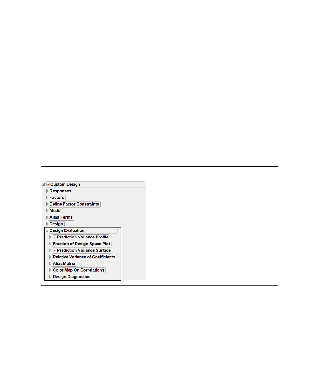
72 Building Custom Designs Chapter 3

Creating a Custom Design

Understanding Design Evaluation

After making the design, you can preview the design and investigate details by looking at various plots and tables that serve as design diagnostic tools.

Although different tools are available depending on the model you specify, most designs display

• the Prediction Variance Profile Plot

• the Fraction of Design Space Plot

• the Prediction Variance Surface Plot

• the Relative Variance of Coefficients and Power Table

•the Alias Matrix

•Design Diagnostic Table

These diagnostic tools are outline nodes beneath the Design Evaluation panel, as shown in Figure 3.9. JMP always provides the Prediction Variance Profile, but the Prediction Surface Plot only appears if there are two or more variables.

Figure 3.9 Custom Design Evaluation and Diagnostic Tools

The Prediction Variance Profile

The example in Figure 3.10 shows the prediction variance profile for a response surface model (RSM) with 2 variables and 8 runs. To see a response surface design similar to this:

1. Chose

DOE > Custom Design.

2. In the Factors panel, add 2 continuous factors.

3. Click

Continue.

4. In the Model panel, click

RSM.

Chapter 3 Building Custom Designs 73

Creating a Custom Design

5. Click Make Design.

6. Open the Prediction Variance Profile.

Figure 3.10 A Factor Design Layout For a Response Surface Design with 2 Variables

The prediction variance for any factor setting is the product of the error variance and a quantity that depends on the design and the factor setting. Before you collect the data the error variance is unknown, so the prediction variance is also unknown. However, the ratio of the prediction variance to the error variance is not a function of the error variance. This ratio, called the relative variance of prediction, depends only on the design and the factor setting and can be calculated before acquiring the data. The prediction variance profile plots the relative variance of prediction as a function of each factor at fixed values of the other factors

After you run the experiment, collect the data, and fit the model, you can estimate the actual variance of prediction at any setting by multiplying the relative variance of prediction by the mean squared error (MSE) of the least squares fit.

It is ideal for the prediction variance to be small throughout the allowable regions of the factors. Generally, the error variance drops as the sample size increases. Comparing the prediction variance profilers for two designs side-by-side, is one way to compare two designs. A design that has lower prediction variance on the average is preferred.

In the profiler, drag the vertical lines in the plot to change the factor settings to different points. Dragging the lines reveals any points that have prediction variances that are larger than you would like.

Another way to evaluate a design, or to compare designs, is to try and minimize the maximum variance. You can use the

Maximize Desirability command on the Prediction Variance Profile title bar to identify the

maximum prediction variance for a model. Consider the Prediction Variance profile for the two-factor RSM model shown in Figure 3.11. The plots on the left are the default plots. The plots on the right identify the factor values where the maximum variance (or worst-case scenario) occur, which helps you evaluate the acceptability of the model.

74 Building Custom Designs Chapter 3

Creating a Custom Design

Figure 3.11 Find Maximum Prediction Variance

The Fraction of Design Space Plot

The Fraction of Design Space plot is a way to see how much of the model prediction variance lies above (or below) a given value. As a simple example, consider the Prediction Variance plot for a single factor quadratic model, shown on the left in Figure 3.12. The Prediction Variance plot shows that 100% of the values are smaller than 0.5. You can move the vertical trace and also see that all the values are above 0.332. The Fraction of Design Space plot displays the same information. The X axis is the proportion of prediction variance values, ranging from 0 to 100%, and the Y axis is the range of prediction variance values. In this simple example, the Fraction of Design plot verifies that 100% of the values are below 0.5 and 0% of the values are below approximately 0.3. You can use the crosshair tool and find the percentage of values for any value of the prediction variance. The example to the right in Figure 3.12 shows that 75% of the prediction variance values are below approximately 0.46.

The Fraction of Design space is most useful when there are multiple factors. It summarizes the prediction variance, showing the fractional design space for all the factors taken together.

Figure 3.12 Variance Profile and Fraction of Design Space

Chapter 3 Building Custom Designs 75

Creating a Custom Design

The Prediction Variance Surface

When there are two or more factors, the Prediction Variance Surface plots the surface of the prediction variance for any two variables. This feature uses the

Graph > Surface Plot platform in JMP, and has all its

functionality. Drag on the plot to rotate and change the perspective. Figure 3.13 shows the Prediction Variance Surface plot for a two-factor RSM model. The factors are on the x and y axes, and the prediction variance is on the z axis. You can clearly see that there are high and low variance areas for both factors. Compare this plot to the Prediction Variance Profile shown in Figure 3.11.

Figure 3.13 Prediction Variance Surface Plot for Two-Factor RSM Model

You can find complete documentation for the Surface Plot platform in Basic Analysis and Graphing.

The Relative Variance of Coefficients and Power Table

Before clicking

Make Table in the custom designer, click the disclosure button ( on Windows and

on the Macintosh) to open Design Evaluation and then again to open the Relative Variance of

Coefficients table.

The Relative Variance of Coefficients table (Figure 3.14) shows the relative variance of all the coefficients for the example RSM custom design (see Figure 3.10). The variances are relative to the error variance, which is unknown before the experiment, and is assumed to be one. Once you complete the experiment and have an estimate for the error variance, you can multiply it by the relative variance to get the estimated variance of the coefficient. The square root of this value should match the standard error of prediction for the coefficient when you fit a model using

The

Power column shows the power of the design as specified to detect effects of a certain size. In the text

Analyze > Fit Model.

edit boxes, you can change the alpha level of the test and the magnitude of the effects compared to the error standard deviation. The alpha level edit box is called Significance Level. The magnitude of the effects edit box is called Signal to Noise Ratio. This is the ratio of the absolute value of the regression parameter to sigma (the square root of the error variance).

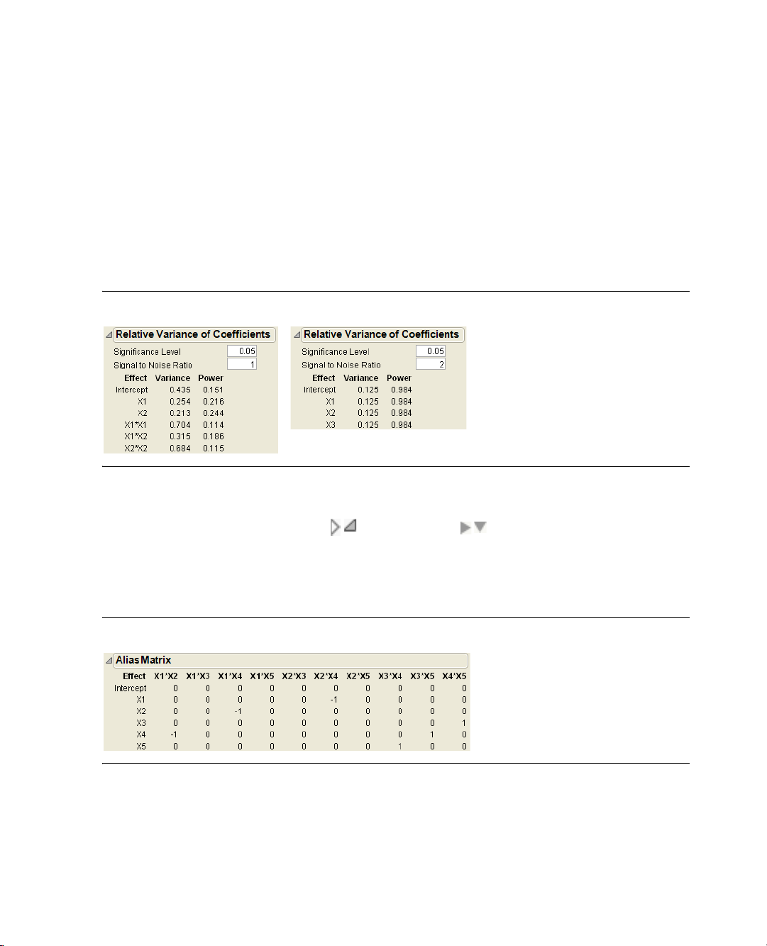
76 Building Custom Designs Chapter 3

Creating a Custom Design

If you enter a smaller alpha (requiring a more significant test), then the power falls. If you increase the magnitude of the effect you want to detect, the power rises.

The power reported is the probability of finding a significant model parameter if the true effect is Signal to Noise Ratio times sigma. The Relative Variance of Coefficients table on the left in Figure 3.14 shows the results for the two-factor RSM model.

As another example, suppose you have a 3-factor 8-run experiment with a linear model and you want to detect any regression coefficient that is twice as large as the error standard deviation, with an alpha level of

0.05. The Relative Variance of Coefficients table on the right in Figure 3.14 shows that the resulting power is 0.984 for all the parameters.

Figure 3.14 Table of Relative Variance of Coefficients

The Alias Matrix (Confounding Pattern)

Click the Alias Matrix disclosure button ( on Windows and on the Macintosh) to open the alias matrix (Figure 3.15).

The alias matrix shows the aliasing between the model terms and the terms you specify in the Alias Terms panel (see “Specifying Alias Terms,” p. 70). It allows you to see the confounding patterns.

Figure 3.15 Alias Matrix

Color Map on Correlations

The Color Map On Correlations panel (see Figure 3.16) shows the correlations between all model terms and alias terms you specify in the Alias Terms panel (see “Specifying Alias Terms,” p. 70). The colors correspond to the absolute value of the correlations.

Chapter 3 Building Custom Designs 77

D-efficiency =

100

-------

X′ X

1 p/





A-efficiency =

100

trace N

X′ X()

1–

()

-----------------------------------------------







G-efficiency =

100

------

---------- -







Creating a Custom Design

Figure 3.16 Color Map of Correlations

The Design Diagnostics Table

Open the Design Diagnostics outline node to display a table with relative D-, G-, and A-efficiencies, average variance of prediction, and length of time to create the design. The design efficiencies are computed as follows:

where

• N

is the number of points in the design

• p is the number of effects in the model including the intercept

• σ

is the maximum standard error for prediction over the design points.

78 Building Custom Designs Chapter 3

Creating a Custom Design

These efficiency measures are single numbers attempting to quantify one mathematical design characteristic. While the maximum efficiency is 100 for any criterion, an efficiency of 100% is impossible for many design problems. It is best to use these design measures to compare two competitive designs with the same model and number of runs rather than as some absolute measure of design quality.

Figure 3.17 Custom Design Showing Diagnostics

Specify Output Options

Use the Output Options panel to specify how you want the output data table to appear.

Figure 3.18 Output Options Panel

Run Order lets you designate the order you want the runs to appear in the data table when it is created.

Choices are:

Keep the Same the rows (runs) in the output table will appear as they do in the Design panel.

Sort Left to Right the rows (runs) in the output table will appear sorted from left to right.

Randomize the rows (runs) in the output table will appear in a random order.

Sort Right to Left the rows (runs) in the output table will appear sorted from right to left.

Randomize within Blocks the rows (runs) in the output table will appear in random order within the

blocks you set up.

Add additional points using options from Make JMP Table from design plus:

Number of Center Points: Specifies additional runs placed at the center of each continuous factor’s

range.

Chapter 3 Building Custom Designs 79

Creating a Custom Design

Number of Replicates:

centerpoints. Type the number of times you want to replicate the design in the associated text box. One replicate doubles the number of runs.

Make the JMP Design Table

When the Design panel shows the layout you want, click Make Table. Parts of the table contain information you might need to continue working with the table in JMP. The upper-left of the design table can have one or more of the following scripts:

• a Screening script runs the generated design.

• a Model script runs the

• a constraint script that shows any model constraints you entered in the Define Factor Constraints panel of the Custom Design dialog.

•a DOE Dialog

script that recreates the dialog used to generate the design table, and regenerates the

design table.

Figure 3.19 Example Design Table

Analyze > Fit Model platform with the model appropriate for the design.

Specify the number of times to replicate the entire design, including

Analyze > Modeling > Screening platform when appropriate for the

1. This area identifies the design type that generated the table. Click Custom Design to edit.

2. Model is a script. Click the red triangle icon and select

Run Script to open the Fit Model dialog, which

is used to generate the analysis appropriate to the design.

3. DOE Dialog is a script. Click the red triangle icon and select

Run Script to recreate the DOE Custom

Dialog and generate a new design table.

80 Building Custom Designs Chapter 3

Creating Random Block Designs

It is often necessary to group the runs of an experiment into blocks. Runs within a block of runs are more homogeneous than runs in different blocks. For example, the experiment described in Goos (2002), describes a pastry dough mixing experiment that took several days to run. It is likely that random day-to-day differences in environmental variables have some effect on all the runs performed on a given day. Random block designs are useful in situations like this, where there is a non-reproducible shock to the system between each block of runs. In Goos (2002), the purpose of the experiment was to understand how certain properties of the dough depend on three factors: feed flow rate, initial moisture content, and rotational screw speed. It was only possible to conduct four runs a day. Because day-to-day variation was likely, it was important to group the runs so that this variation would not compromise the information about the three factors. Thus, blocking the runs into groups of four was necessary. Each day's experimentation was one block. The factor, Day, is an example of a random block factor.

To create a random block, use the custom design and enter responses and factors, and define your model as usual. In the Design Generation panel, check the Group runs into random blocks of size check box and enter the number of runs you want in each block. When you select or enter the sample size, the number of runs specified are assigned to the blocks.

Figure 3.20 Assigning Runs to Blocks

In this example, the Design Generation Panel shown here designates four runs per block, and the number of runs (16) indicates there will be four days (blocks) of 4 runs. If the number of runs is not an even multiple of the random block size, some blocks will have a fewer runs than others.

Creating Split Plot Designs

Split plot experiments happen when it is convenient to run an experiment in groups of runs (called whole plots) where one or more factors stay constant within each group. Usually this is because these factors are difficult or expensive to change from run to run. JMP calls these factors usually how split plotting arises in industrial practice.

In a completely randomized design, any factor can change its setting from one run to the next. When certain factors are hard to change, the completely randomized design may require more changes in the settings of hard-to-change factors than desired.

Hard to change because this is

Chapter 3 Building Custom Designs 81

X′V1–X

Creating Split-Split Plot Designs

If you know that a factor or two are difficult to change, then you can set the Changes setting of a factor from the default of

Easy to Hard. Before making the design, you can set the number of whole plots you are

willing to run.

For an example of creating a split plot design, see “Creating a Design with Two Hard-to-Change Factors:

Split Plot,” p. 54.

To create a split plot design using the custom designer:

1. In the factors table there is a column called however, you click in the changes area for a factor, you can choose to make the factor

2. Once you finish defining the factors and click continue, you see an edit box for supplying the number of whole plots. You can supply any value as long as it is above the minimum necessary to fit all the model parameters. You can also leave this field empty. In this case, JMP chooses a number of whole plots to minimize the omnibus uncertainty of the fixed parameters.

Note: If you enter a missing value in the Number of Whole Plots edit box, then JMP considers many different numbers of whole plots and chooses the number that maximizes the information about the coefficients in the model. It maximizes the determinant of where V matrix of the responses. The matrix, V, is a function of how many whole plots there are, so changing the number of whole plots changes V, which can make a difference in the amount of information a design contains.

To create a split plot design every time you use a certain factor, save steps by setting up that factor to be “hard” in all experiments. See “Identify Factor Changes Column Property,” p. 98, for details.

Creating Split-Split Plot Designs

Split-split plot designs are a three stratum extension of split plot designs. Now there are factors that are Very-Hard-to-change, Hard-to-change, and Easy-to-change. Here, in the top stratum, the Very-Hard-tochange factors stay fixed within each whole plot. In the middle stratum the Hard-to-change factors stay fixed within each subplot. Finally, the Easy-to-change factors may vary (and should be reset) between runs within a subplot. This structure is natural when an experiment covers three processing steps. The factors in the first step are Very-Hard-to-change in the sense that once the material passes through the first processing stage, these factor settings are fixed. Now the material passes to the second stage where the factors are all Hard-to-change. In the third stage, the factors are Easy-to-change.

Changes. By default, changes are Easy for all factors. If,

Hard to change.

is the inverse of the variance

Schoen (1999) provides an example of three-stage processing involving the production of cheese that leads to a split-split plot design. The first processing step is milk storage. Typically milk from one storage facility provides the raw material for several curds processing units—the second processing stage. Then the curds are further processed to yield individual cheeses.

In a split-split plot design the material from one processing stage passes to the next stage in such a way that nests the subplots within a whole plot. In the example above, milk from a storage facility becomes divided into two curds processing units. Each milk storage tank provided milk to a different set of curds processors. So, the curds processors were nested within the milk storage unit.

82 Building Custom Designs Chapter 3

Creating Strip Plot Designs

Figure 3.21 shows an example of how factors might be defined for the cheese processing example.

Figure 3.21 Example of Split-Split Response and Factors in Custom Designer Dialog

Creating Strip Plot Designs

In a strip plot design it is possible to reorder material between processing stages. Suppose units are labelled and go through the first stage in a particular order. If it is possible to collect all the units at the end of the first stage and reorder them for the second stage process, then the second stage variables are not nested within the blocks of the first stage variables. For example, in semiconductor manufacturing a boat of wafers may go through the first processing step together. However, after this step, the wafers in a given boat may be divided among many boats for the second stage.

To set up a strip plot design, enter responses and factors as usual, designating factors as Very Hard, Hard, or Easy to change. Then, in the Design Generation panel, check the box that says

can vary independently of Very Hard to change factors

, as shown in Figure 3.22. Note that the Design

Hard to change factors

Generation panel specified 6 whole plots, 12 subplots, and 24 runs.

When you click

Make Design, the design table on the right in Figure 3.22 lists the run with subplots that

are not nested in the whole plots.

Chapter 3 Building Custom Designs 83

Special Custom Design Commands

Figure 3.22 Example of Strip Split Factors and Design Generation panel in Custom Designer Dialog

Special Custom Design Commands

After you select DOE > Custom Design, click the red triangle icon on the title bar to see the list of commands available to the Custom designer (Figure 3.23). The commands found on this menu vary, depending on which DOE command you select. However, the commands to save and load responses and factors, the command to set the random seed, and the command to simulate responses are available to all designers. You should examine the red triangle menu for each designer you use to determine which commands are available. If a designer has additional commands, they are described in the appropriate chapter.

84 Building Custom Designs Chapter 3

Special Custom Design Commands

Figure 3.23 Click the Red Triangle Icon to Reveal Commands

The following sections describe these menu commands and how to use them.

Save Responses and Save Factors

If you plan to do further experiments with factors and/or responses to which you have given meaningful names and values, you can save them for later use.

To save factors or responses:

1. Select a design type from the DOE menu.

2. Enter the factors and responses into the appropriate panels (see “Enter Responses and Factors into the

Custom Designer,” p. 65, for details).

3. Click the red triangle icon on the title bar and select

Save Responses creates a data table containing a row for each response with a column called

Response Name that identifies the responses. Four additional columns identify more information

about the responses:

Save Factors creates a data table containing a column for each factor and a row for each factor level.

The columns have two column properties (noted with asterisks icons in the column panel). These properties include:

Design Role that identifies the factor as a DOE factor and lists its type (continuous, categorical,

blocking, and so on).

Factor Changes that identifies how difficult it is to change the factor level. Factor Changes options

are

Easy, Hard, and Very H ard.

4. Save the data table.

Lower Limit, Upper Limit, Response Goal, and Importance.

Save Responses or Save Factors.

Sas DESIGN OF EXPERIMENTS RELEASE 9 User Manual

Specifications and Main Features

Frequently Asked Questions

User Manual

Introduction to Designing Experiments

About Designing Experiments

My First Experiment

The Situation

Step 1: Design the Experiment

Define the Responses: Popped Kernels and Total Kernels

Define the Factors: Time, Power, and Brand

Step 2: Define Factor Constraints

Step 3: Add Interaction Terms

Step 4: Determine the Number of Runs

Step 5: Check the Design

Step 6: Gather and Enter the Data

Step 7: Analyze the Results

Examples Using the Custom Designer

Creating Screening Experiments

Creating a Main-Effects-Only Screening Design

Creating a Screening Design to Fit All Two-Factor Interactions

A Compromise Design Between Main Effects Only and All Interactions

Creating ‘Super’ Screening Designs

The Need for Supersaturated Designs

Example: Twelve Factors in Eight Runs

Screening Designs with Flexible Block Sizes

Checking for Curvature Using One Extra Run

Creating Response Surface Experiments

Exploring the Prediction Variance Surface

Introducing I-Optimal Designs for Response Surface Modeling

A Three-Factor Response Surface Design

Response Surface with a Blocking Factor

Creating Mixture Experiments

Mixtures Having Nonmixture Factors

Experiments that are Mixtures of Mixtures

Special-Purpose Uses of the Custom Designer

Designing Experiments with Fixed Covariate Factors

Creating a Design with Two Hard-to-Change Factors: Split Plot

Technical Discussion

Building Custom Designs

Creating a Custom Design

Enter Responses and Factors into the Custom Designer

How to Enter Responses

Specifying Response Goal Types and Lower and Upper Limits

Understanding Response Importance Weights

Adding Simulated Responses, If Desired

How to Enter Factors

Factors that are Easy, Hard, or Very Hard, to Change: Creating Optimal Split-Plot and Split-Split-Plot Designs

Defining Factor Constraints, If Necessary

Describe the Model

Specifying Alias Terms

Select the Number of Runs

Understanding Design Evaluation

The Prediction Variance Profile

The Fraction of Design Space Plot

The Prediction Variance Surface

The Relative Variance of Coefficients and Power Table

The Alias Matrix (Confounding Pattern)

Color Map on Correlations

The Design Diagnostics Table

Specify Output Options

Make the JMP Design Table

Creating Random Block Designs

Creating Split Plot Designs

Creating Split-Split Plot Designs

Creating Strip Plot Designs

Special Custom Design Commands

Save Responses and Save Factors