

Page 1

Tutorial
■ SAP BusinessObjects Data Services XI 4.0 (14.0.0)
2010-12-02
Page 2

Copyright
© 2010 SAP AG. All rights reserved.SAP, R/3, SAP NetWeaver, Duet, PartnerEdge, ByDesign, SAP
Business ByDesign, and other SAP products and services mentioned herein as well as their respective
logos are trademarks or registered trademarks of SAP AG in Germany and other countries. Business
Objects and the Business Objects logo, BusinessObjects, Crystal Reports, Crystal Decisions, Web
Intelligence, Xcelsius, and other Business Objects products and services mentioned herein as well
as their respective logos are trademarks or registered trademarks of Business Objects S.A. in the
United States and in other countries. Business Objects is an SAP company.All other product and
service names mentioned are the trademarks of their respective companies. Data contained in this
document serves informational purposes only. National product specifications may vary.These materials
are subject to change without notice. These materials are provided by SAP AG and its affiliated
companies ("SAP Group") for informational purposes only, without representation or warranty of any
kind, and SAP Group shall not be liable for errors or omissions with respect to the materials. The
only warranties for SAP Group products and services are those that are set forth in the express
warranty statements accompanying such products and services, if any. Nothing herein should be
construed as constituting an additional warranty.
2010-12-02
Page 3

Contents
Introduction.............................................................................................................................9Chapter 1
1.1
1.2
1.3
1.4
1.4.1
1.4.2
1.4.3
1.5
1.6
1.6.1
1.6.2
2.1
2.2
2.3
2.4
2.4.1
2.4.2
2.5
2.6
2.6.1
2.6.2
2.7
2.8
Audience and assumptions.......................................................................................................9
SAP BusinessObjects information resources...........................................................................9
Tutorial objectives..................................................................................................................10
Tutorial prerequisites..............................................................................................................11
Preparation for this tutorial.....................................................................................................11
Environment required.............................................................................................................12
Tutorial setup.........................................................................................................................12
Tutorial structure....................................................................................................................19
Exiting the tutorial...................................................................................................................20
To exit the tutorial..................................................................................................................20
To resume the tutorial............................................................................................................21
Product Overview .................................................................................................................23Chapter 2
Product features....................................................................................................................23
Product components..............................................................................................................24
Using the product..................................................................................................................25
System configurations............................................................................................................26
Windows implementation.......................................................................................................27
UNIX implementation.............................................................................................................27
The Designer window.............................................................................................................27
SAP BusinessObjects Data Services objects.........................................................................28
Object hierarchy.....................................................................................................................29
Object-naming conventions....................................................................................................32
New terms.............................................................................................................................32
Section summary and what to do next....................................................................................34
3.1
3.2
3.2.1
3.2.2
Defining Source and Target Metadata .................................................................................35Chapter 3
Logging in to the Designer.....................................................................................................35
Defining a datastore...............................................................................................................36
To define a datastore for the source (ODS) database............................................................36
To define a datastore for the target database.........................................................................38
2010-12-023
Page 4

Contents
3.3
3.3.1
3.3.2
3.4
3.4.1
3.5
3.6
4.1
4.2
4.2.1
4.3
4.3.1
4.4
4.4.1
4.5
4.5.1
4.5.2
4.5.3
4.5.4
4.6
4.7
4.8
4.9
4.10
Importing metadata................................................................................................................38
To import metadata for ODS source tables ...........................................................................38
To import metadata for target tables......................................................................................39
Defining a file format..............................................................................................................39
To define a file format.............................................................................................................40
New terms.............................................................................................................................41
Summary and what to do next................................................................................................42
Populating the SalesOrg Dimension from a Flat File............................................................43Chapter 4
Objects and their hierarchical relationships.............................................................................43
Adding a new project..............................................................................................................44
To add a new project..............................................................................................................44
Adding a job...........................................................................................................................44
To add a new batch job..........................................................................................................44
Adding a work flow.................................................................................................................45
To add a work flow.................................................................................................................46
About data flows....................................................................................................................47
Adding a data flow..................................................................................................................47
Defining the data flow............................................................................................................48
Validating the data flow..........................................................................................................51
Addressing errors..................................................................................................................52
Saving the project..................................................................................................................52
To execute the job.................................................................................................................53
About deleting objects...........................................................................................................55
New terms.............................................................................................................................55
Summary and what to do next................................................................................................56
5.1
5.1.1
5.2
5.2.1
5.3
5.3.1
5.3.2
5.3.3
5.3.4
5.4
5.5
Populating the Time Dimension Using a Transform..............................................................57Chapter 5
Retrieving the project.............................................................................................................57
To open the Class_Exercises project.....................................................................................58
Adding the job and data flow..................................................................................................58
To add the job and data flow..................................................................................................58
Defining the time dimension data flow....................................................................................58
To specify the components of the time data flow...................................................................59
To define the flow of data.......................................................................................................59
To define the output of the Date_Generation transform.........................................................59
To define the output of the query...........................................................................................60
Saving and executing the job..................................................................................................62
Summary and what to do next................................................................................................62
2010-12-024
Page 5

Contents
Populating the Customer Dimension from a Relational Table..............................................63Chapter 6
6.1
6.1.1
6.1.2
6.2
6.2.1
6.3
6.3.1
6.3.2
6.4
6.4.1
6.5
6.6
6.6.1
6.6.2
6.6.3
6.7
7.1
7.1.1
7.2
7.2.1
7.3
7.3.1
7.3.2
7.4
7.4.1
7.5
7.5.1
7.6
7.6.1
7.6.2
7.7
Adding the CustDim job and work flow...................................................................................63
To add the CustDim job.........................................................................................................63
To add the CustDim work flow...............................................................................................64
Adding the CustDim data flow................................................................................................64
To add the CustDim data flow object.....................................................................................64
Defining the CustDim data flow..............................................................................................64
To bring the objects into the data flow....................................................................................64
To define the query................................................................................................................65
Validating the CustDim data flow...........................................................................................66
To verify that the data flow has been constructed properly.....................................................66
Executing the CustDim job.....................................................................................................66
Using the interactive debugger...............................................................................................67
To set a breakpoint in a data flow...........................................................................................67
To use the interactive debugger.............................................................................................68
To set a breakpoint condition.................................................................................................69
Summary and what to do next................................................................................................70
Populating the Material Dimension from an XML File..........................................................71Chapter 7
Adding MtrlDim job, work and data flows...............................................................................71
To add the MtrlDim job objects..............................................................................................72
Importing a document type definition......................................................................................72
To import the mtrl.dtd.............................................................................................................72
Defining the MtrlDim data flow...............................................................................................72
To add the objects to the data flow........................................................................................73
To define the details of qryunnest..........................................................................................73
Validating the MtrlDim data flow.............................................................................................75
To verify that the data flow has been constructed properly.....................................................75
Executing the MtrlDim job......................................................................................................75
To execute the job.................................................................................................................75
Leveraging the XML_Pipeline ................................................................................................76
To setup a job and data flow that uses the XML_Pipeline transform.......................................76
To define the details of XML_Pipeline and Query_Pipeline......................................................77
Summary and what to do next................................................................................................79
8.1
8.2
8.2.1
Populating the Sales Fact Table from Multiple Relational Tables.........................................81Chapter 8
Exercise overview..................................................................................................................82
Adding the SalesFact job, work flow, and data flow................................................................82
To add the SalesFact job objects...........................................................................................82
2010-12-025
Page 6

Contents
8.3
8.3.1
8.4
8.4.1
8.5
8.5.1
8.6
8.7
8.8
8.8.1
8.8.2
8.9
9.1
9.2
9.2.1
9.2.2
9.3
9.3.1
9.3.2
9.3.3
9.3.4
9.4
9.4.1
9.4.2
9.4.3
9.5
Defining the SalesFact data flow............................................................................................82
To define the data flow that will generate the sales fact table.................................................83
Defining the details of the Query transform............................................................................83
To define the details of the query, including the join between source tables...........................83
Defining the details of the lookup_ext function.......................................................................84
To use a lookup_ext function for order status.........................................................................85
Validating the SalesFact data flow..........................................................................................86
Executing the SalesFact job...................................................................................................87
Using metadata reports..........................................................................................................87
Enabling metadata reporting...................................................................................................87
Viewing Impact and Lineage Analysis.....................................................................................88
Summary and what to do next................................................................................................91
Changed-Data Capture.........................................................................................................93Chapter 9
Exercise overview..................................................................................................................93
Adding and defining the initial-load job....................................................................................94
Adding the job and defining global variables...........................................................................94
Adding and defining the work flow..........................................................................................95
Adding and defining the delta-load job....................................................................................97
To add the delta-load data flow...............................................................................................97
To add the job and define the global variables........................................................................98
To add and define the work flow.............................................................................................98
To define the scripts...............................................................................................................99
Executing the jobs..................................................................................................................99
To execute the initial-load job.................................................................................................99
To change the source data...................................................................................................100
To execute the delta-load job...............................................................................................100
Summary and what to do next..............................................................................................101
10.1
10.1.1
10.2
10.2.1
10.2.2
10.3
10.4
10.4.1
10.5
Data Assessment................................................................................................................103Chapter 10
Viewing profile statistics ......................................................................................................103
To obtain profile statistics....................................................................................................104
Defining a validation transform based on data profile statistics.............................................105
To set up the job and data flow that will validate the data format..........................................105
To define the details of the Validation transform to replace incorrectly formatted data ........106
To audit a data flow..............................................................................................................107
Viewing audit details in Operational Dashboard reports........................................................110
To view audit details in the Operational Dashboard..............................................................110
Summary and what to do next..............................................................................................111
2010-12-026
Page 7

Contents
Recovery Mechanisms........................................................................................................113Chapter 11
11.1
11.2
11.2.1
11.3
11.3.1
11.3.2
11.3.3
11.3.4
11.4
11.5
11.5.1
11.6
11.7
12.1
12.2
12.3
12.3.1
12.3.2
12.3.3
12.3.4
12.4
12.4.1
12.4.2
12.4.3
12.4.4
12.4.5
12.4.6
12.4.7
12.4.8
12.4.9
12.4.10
12.4.11
12.5
Creating a recoverable work flow manually...........................................................................113
Adding the job and defining local variables...........................................................................113
To add the job and define local variables..............................................................................114
Specifying a recoverable job................................................................................................114
Creating the script that determines the status......................................................................115
Defining the recoverable data flow with a conditional............................................................116
Adding the script that updates the status.............................................................................118
Specifying job execution order.............................................................................................119
Status of the exercise..........................................................................................................119
Executing the job..................................................................................................................119
To execute the job...............................................................................................................119
Data Services automated recovery properties......................................................................120
Summary and what to do next..............................................................................................120
Multiuser Development.......................................................................................................121Chapter 12
Introduction..........................................................................................................................121
Exercise overview................................................................................................................122
Preparation..........................................................................................................................122
To create a central repository...............................................................................................123
Creating two local repositories.............................................................................................124
Associating repositories to your job server..........................................................................124
Defining connections to the central repository.....................................................................125
Working in a multiuser environment......................................................................................126
To import objects into your local repository .........................................................................126
Activating a connection to the central repository..................................................................127
Adding objects to the central repository...............................................................................128
Checking out objects from the central repository.................................................................130
Checking in objects to the central repository........................................................................131
Undoing check out...............................................................................................................132
Comparing objects...............................................................................................................133
Checking out without replacement.......................................................................................135
Getting objects....................................................................................................................137
Using filtering.......................................................................................................................138
Deleting objects...................................................................................................................139
Summary and what to do next..............................................................................................140
13.1
Extracting SAP Application Data.........................................................................................141Chapter 13
Defining an SAP Applications datastore...............................................................................141
2010-12-027
Page 8

Contents
13.2
13.3
13.3.1
13.3.2
13.3.3
13.3.4
13.3.5
13.3.6
13.4
13.4.1
13.4.2
13.4.3
13.4.4
13.5
13.5.1
13.5.2
13.5.3
13.5.4
13.6
13.7
To import metadata for individual SAP application source tables..........................................142
Repopulating the customer dimension table.........................................................................143
Adding the SAP_CustDim job, work flow, and data flow.......................................................143
Defining the SAP_CustDim data flow...................................................................................144
Defining the ABAP data flow................................................................................................145
Validating the SAP_CustDim data flow.................................................................................149
Executing the SAP_CustDim job..........................................................................................149
About ABAP job execution errors.........................................................................................150
Repopulating the material dimension table............................................................................150
Adding the SAP_MtrlDim job, work flow, and data flow........................................................151
Defining the DF_SAP_MtrlDim data flow..............................................................................151
Defining the data flow..........................................................................................................152
Executing the SAP_MtrlDim job...........................................................................................155
Repopulating the SalesFact table.........................................................................................156
Adding the SAP_SalesFact job, work flow, and data flow.....................................................156
Defining the DF_SAP_SalesFact data flow...........................................................................156
Defining the ABAP data flow................................................................................................157
Validating the SAP_SalesFact data flow and executing the job.............................................163
New Terms..........................................................................................................................163
Summary.............................................................................................................................164
Running a Real-time Job in Test Mode...............................................................................165Chapter 14
14.1
Index 167
Exercise...............................................................................................................................165
2010-12-028
Page 9

Introduction
Introduction
Welcome to the
The software is a component of the SAP BusinessObjects information management solutions and
allows you to extract and integrate data for analytical reporting and e-business.
Exercises in this tutorial introduce concepts and techniques to extract, transform, and load batch data
from flat-file and relational database sources for use in a data warehouse. Additionally, you can use
the software for real-time data extraction and integration. Use this tutorial to gain practical experience
using software components including the Designer, repositories, and Job Servers.
SAP BusinessObjects information management solutions also provide a number of Rapid Marts
packages, which are predefined data models with built-in jobs for use with business intelligence (BI)
and online analytical processing (OLAP) tools. Contact your sales representative for more information
about Rapid Marts.
Tutorial
. This tutorial introduces core features of SAP BusinessObjects Data Services.
1.1 Audience and assumptions
This tutorial assumes that:
• You are an application developer or database administrator working on data extraction, data
warehousing, data integration, or data quality.
• You understand your source data systems, DBMS, business intelligence, and e-business messaging
concepts.
• You understand your organization's data needs.
• You are familiar with SQL (Structured Query Language).
• You are familiar with Microsoft Windows.
1.2 SAP BusinessObjects information resources
A global network of SAP BusinessObjects technology experts provides customer support, education,
and consulting to ensure maximum information management benefit to your business.
Useful addresses at a glance:
2010-12-029
Page 10
Introduction
ContentAddress
Customer Support, Consulting, and Education
services
http://service.sap.com/
SAP BusinessObjects Data Services Community
http://www.sdn.sap.com/irj/sdn/ds
Forums on SCN (SAP Community Network )
http://forums.sdn.sap.com/forum.jspa?foru
mID=305
Blueprints
http://www.sdn.sap.com/irj/boc/blueprints
Information about SAP Business User Support
programs, as well as links to technical articles,
downloads, and online forums. Consulting services
can provide you with information about how SAP
BusinessObjects can help maximize your information management investment. Education services
can provide information about training options and
modules. From traditional classroom learning to
targeted e-learning seminars, SAP BusinessObjects
can offer a training package to suit your learning
needs and preferred learning style.
Get online and timely information about SAP BusinessObjects Data Services, including tips and tricks,
additional downloads, samples, and much more.
All content is to and from the community, so feel
free to join in and contact us if you have a submission.
Search the SAP BusinessObjects forums on the
SAP Community Network to learn from other SAP
BusinessObjects Data Services users and start
posting questions or share your knowledge with the
community.
Blueprints for you to download and modify to fit your
needs. Each blueprint contains the necessary SAP
BusinessObjects Data Services project, jobs, data
flows, file formats, sample data, template tables,
and custom functions to run the data flows in your
environment with only a few modifications.
http://help.sap.com/businessobjects/
Supported Platforms (Product Availability Matrix)
https://service.sap.com/PAM
1.3 Tutorial objectives
SAP BusinessObjects product documentation.Product documentation
Get information about supported platforms for SAP
BusinessObjects Data Services.
Use the search function to search for Data Services.
Click the link for the version of Data Services you
are searching for.
2010-12-0210
Page 11

Introduction
The intent of this tutorial is to introduce core Designer functionality.
After completing this tutorial you should be able to:
• Describe the process for extracting, transforming, and loading data using SAP BusinessObjects
Data Services
• Identify Data Services objects
• Define Data Services objects to:
• Extract flat-file, XML, and relational data from your sources
• Transform the data to suit your needs
• Load the data to your targets
• Use Data Services features and functions to:
• Recover from run-time errors
• Capture changed data
• Verify and improve the quality of your source data
• Run a real-time job
• View and print metadata reports
• Examine data throughout a job using the debugger
• Set up a multiuser development environment
1.4 Tutorial prerequisites
This section provides a high-level description of the steps you need to complete before you begin the
tutorial exercises.
1.4.1 Preparation for this tutorial
Read the sections on logging in to the Designer and the Designer user interface in the
BusinessObjects Data Services Designer Guide
including terms and concepts relevant to this tutorial.
SAP
to get an overview of the Designer user interface
This tutorial also provides a high-level summary in the next section,
Product Overview
.
2010-12-0211
Page 12
Introduction
1.4.2 Environment required
To use this tutorial, you must have Data Services running on a supported version of Windows XP or
Windows Server 2003 and a supported RDBMS (such as Oracle, IBM DB2, Microsoft SQL Server, or
Sybase ASE).
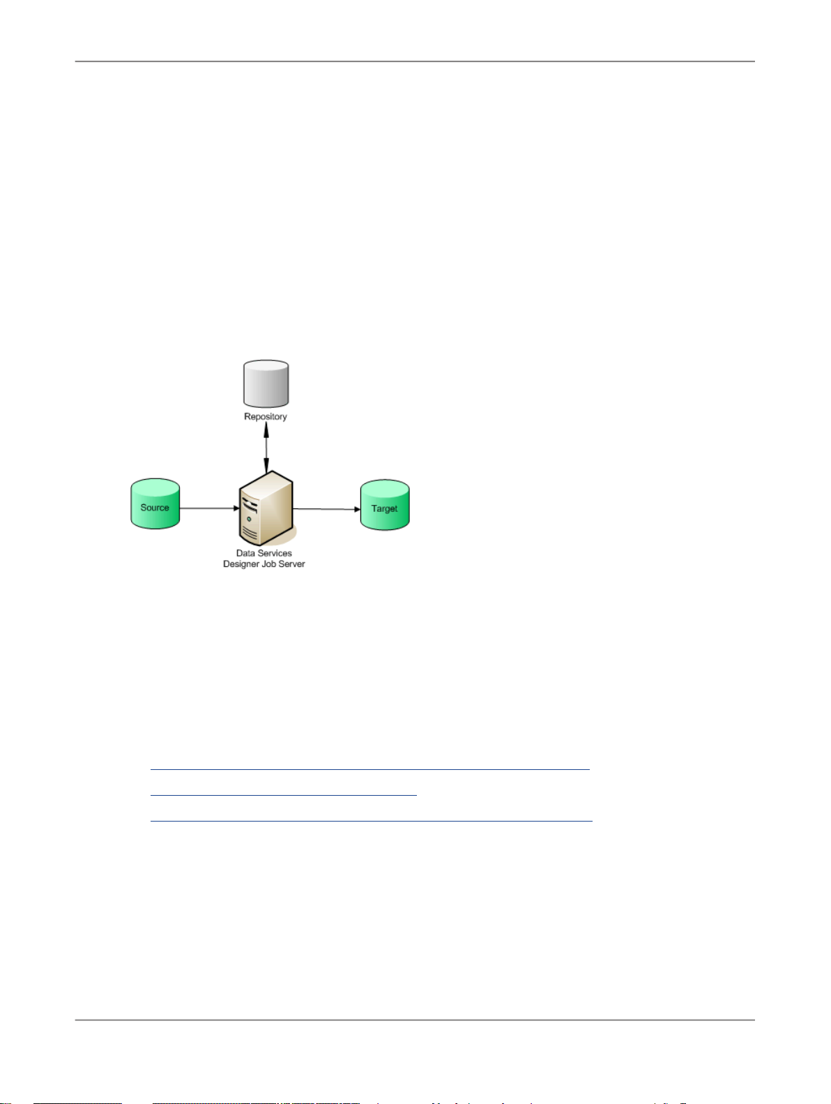
You can install Data Services product components (Designer, Administrator, Job Server, Access Server)
on a single computer or distribute them across multiple computers. In the simplest case, all components
in the following diagram can reside on the same computer.
1.4.3 Tutorial setup
Ensure you have access to a RDBMS; contact your system administrator for assistance.
To set up your computer for this tutorial you must do the following tasks:
• Create repository, source, and target databases on an existing RDBMS
• Install SAP BusinessObjects Data Services
• Run the provided SQL scripts to create sample source and target tables
The following sections describe each of these tasks.
1.4.3.1 Create repository, source, and target databases on an existing RDBMS
2010-12-0212
Page 13
Introduction
1.
Log in to your RDBMS.
2.
(Oracle only). Optionally create a service name alias.
Set the protocol to TCP/IP and enter a service name; for example, training.sap. This can act as your
connection name.
3.
Create three databases—for your repository, source operational data store (ODS), and target. For
each, you must create a user account and password.
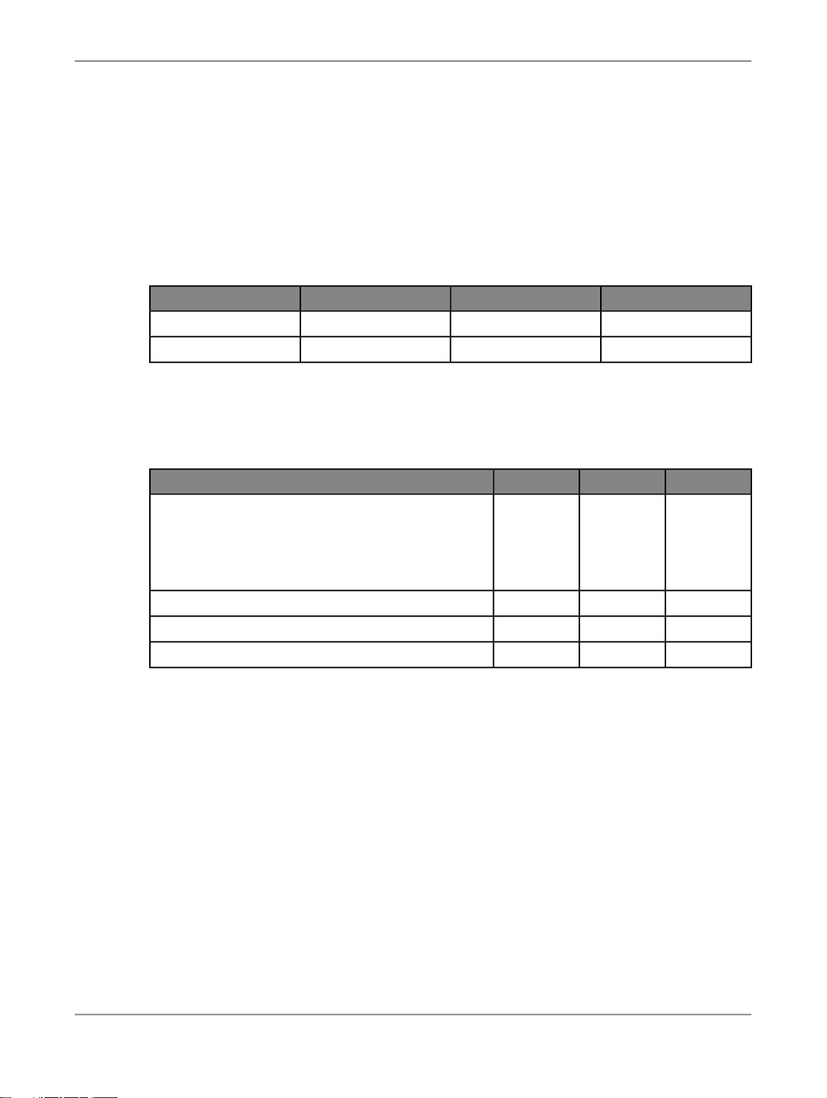
The recommended values used in the tutorial SQL scripts are:
TargetSourceRepository
targetodsrepoUser name
targetodsrepoPassword
4.
Grant access privileges for the user account. For example for Oracle, grant CONNECT and
RESOURCE roles.
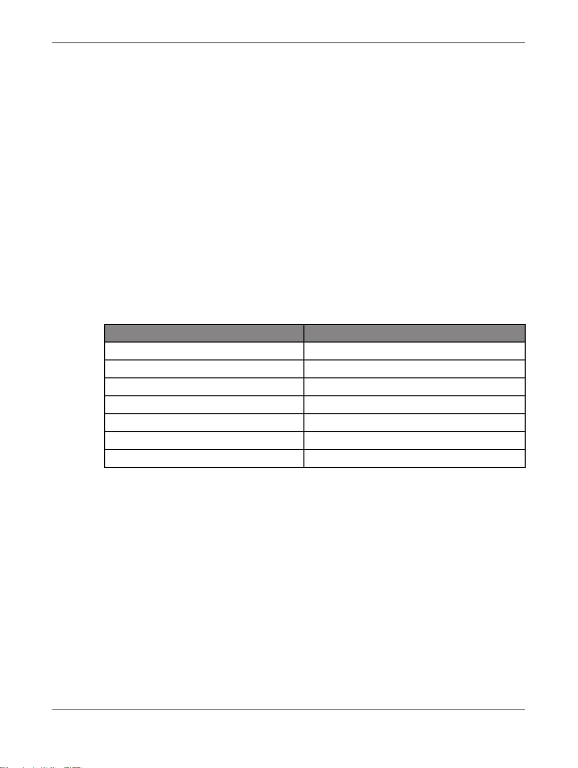
5.
Make a note of the connection names, database versions, user names and passwords in the following
table. You will be asked to refer to this information throughout the tutorial.
TargetSourceRepositoryValue
Database connection name (Oracle) OR
Database server name AND
Database name (MS-SQL Server)
Database version
User name
Password
1.4.3.2 Install a Central Management Server (CMS)
SAP BusinessObjects Data Services requires a Central Managment Server (CMS) provided by SAP
BusinessObjects Enterprise or Information platform services 4.0.
For detailed information about system requirements, configuration, and installation for Information
platform services 4.0, see the “Installing Information platform services 4.0” section of the
Guide for Windows
.
Installation
For detailed information about system requirements, configuration, and installation for SAP
BusinessObjects Enterprise, see the
SAP BusinessObjects Enterprise Installation Guide
.
2010-12-0213
Page 14

Introduction
Note:
During installation, make a note of the administrator user name and password for the SAP
BusinessObjects Enterprise or Information platform services 4.0 system. You will be asked to enter it
to complete the setup of the tutorial.
1.4.3.2.1 To log in to the Central Management Console
To configure user accounts and define Data Services repositories, log in to the Central Management
Console (CMC).
1.
Navigate to http://<hostname>:8080/BOE/CMC/, where <hostname> is the name of the
machine where you installed SAP BusinessObjects Enterprise or Information platform services 4.0.
2.
Enter the username, password, and authentication type for your CMS user.
3.
Click Log On.
The Central Management Console main screen is displayed.
1.4.3.3 Install SAP BusinessObjects Data Services
For detailed information about system requirements, configuration, and installing on Windows or UNIX,
See the
Be prepared to enter the following information when installing the software:
• Your Windows domain and user name
• Your Windows password
• Your Windows computer name and host ID
• Product keycode
• Connection information for the local repository and Job Server
When you install the software, it configures a Windows service for the Job Server. To verify that the
service is enabled, open the Services Control Panel and ensure that all Data Services services are
configured for a Status of Started and Startup Type Automatic.
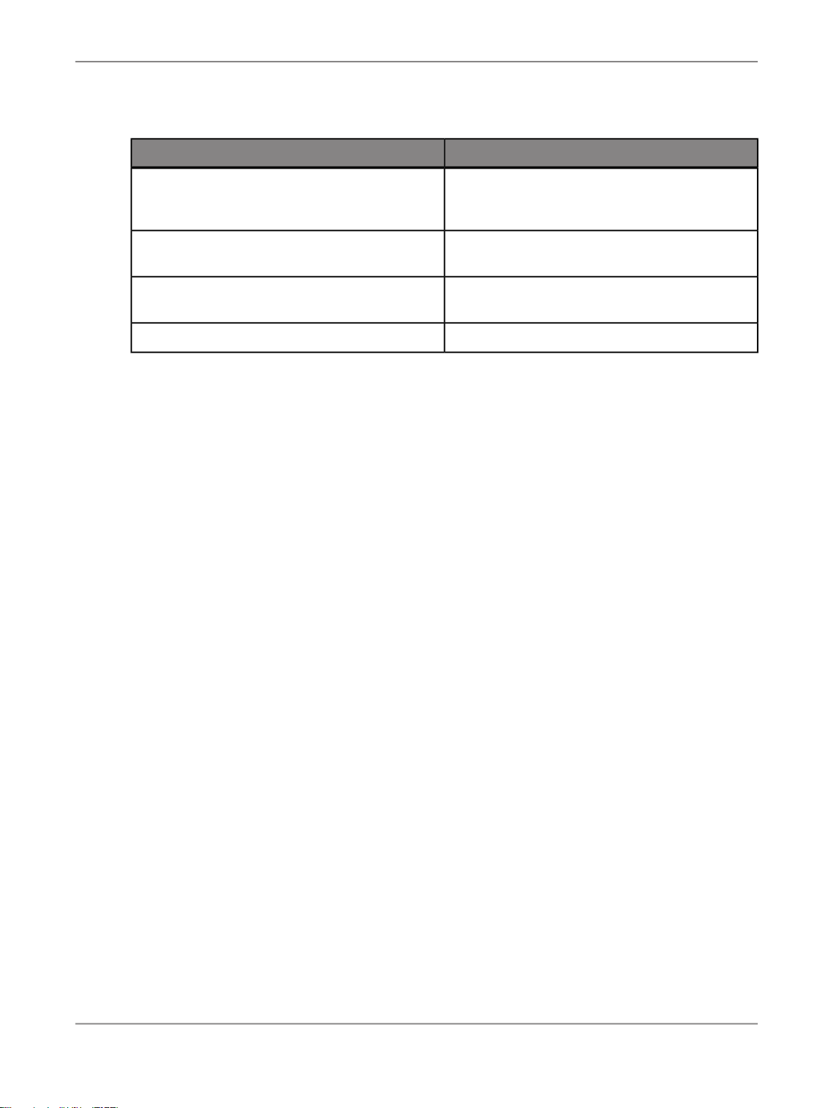
The default installation creates the following entries in the Start > Programs > SAP BusinessObjects
Data Services XI 4.0 menu:
Data ServicesLocale Selector
Installation Guide for WindowsorInstallation Guide for UNIX
FunctionCommand
Opens the Designer.Data ServicesDesigner
Allows you to specify the language, territory, and
code page to use for the repository connection
for Designer and to process job data
.
2010-12-0214
Page 15
Introduction
Data ServicesManagement Console
FunctionCommand
Opens a launch page for the Data Services web
applications including the Administrator and
metadata and data quality reporting tools.
Data ServicesRepository Manager
Data ServicesServer Manager
Opens a dialog box that you can use to update
repository connection information.
Opens a dialog box that you can use to configure
Job Servers and Access Servers.
Displays license information.SAP BusinessObjectsLicense Manager
1.4.3.3.1 To create a local repository
1.
Open the Repository Manager.
2.
Choose Local as the repository type.
3.
Enter the connection information for the local repository database that you created.
4.
Type repo for both User and Password.
5.
Click Create.
After creating the repository, you need to define a Job Server and associate the repository with it. You
can also optionally create an Access Server if you want to use web-based batch job administration.
1.4.3.3.2 To define a job server and associate your repository
1.
Open the Server Manager.
2.
In the Job Server tab of the Server Manager window, click Configuration Editor.
3.
In the "Job Server Configuration Editor" window, click Add to add a Job Server.
4.
In the "Job Server Properties" window:
a. Enter a unique name in Job Server name.
b. For Job Server port, enter a port number that is not used by another process on the computer.
If you are unsure of which port number to use, increment the default port number.
c. You do not need to complete the other job server properties to run the exercises in this Tutorial.
5.
Under Associated Repositories, enter the local repository to associate with this Job Server. Every
Job Server must be associated with at least one local repository.
a. Click Add to associate a new local or profiler repository with this Job Server.
b. Under Repository information enter the connection information for the local repository database
that you created.
c. Type repo for both Username and Password.
d. Select the Default repository check box if this is the default repository for this Job Server. You
cannot specify more than one default repository.
e. Click Apply to save your entries. You should see <database_server>_repo_repo in the list
of Associated Repositories.
2010-12-0215
Page 16
Introduction
6.
Click OK to close the "Job Server Properties" window.
7.
Click OK to close the "Job Server Configuration Editor" window.
8.
Click Close and Restart in the Server Manager.
9.
Click OK to confirm that you want to restart the Data Services Service.
1.4.3.3.3 To create a new Data Services user account
Before you can log in to the Designer, you need to create a user account on the Central Management
Server (CMS).
1.
Log in to the Central Management Console (CMC) using the Administrator account you created
during installation.
2.
Click Users and Groups.
The user management screen is displayed.
3.
Click Manage > New > New User.
The "New User" screen is displayed.
4.
Enter user details for the new user account:
ValueField
EnterpriseAuthentication Type
tutorial_userAccount Name
Tutorial UserFull Name
User created for the Data Services tutorial.Description
tutorial_passPassword
CheckedPassword never expires
UncheckedUser must change password at next logon
5.
Click Create & Close.
The user account is created and the "New User" screen is closed.
6.
Add your user to the necessary Data Services user groups:
a. Click User List.
b. Select tutorial_user in the list of users.
c. Choose Actions > Join Group.
The "Join Group" screen is displayed.
d. Select all the Data Services groups and click >.
Caution:
This simplifies the process for the purposes of the tutorial. In a production environment, you
should plan user access more carefully. For more information about user security, see the
Administrator's Guide
.
The Data Services groups are moved to the Destination Groups area.
2010-12-0216
Page 17

Introduction
e. Click OK.
The "Join Group" screen is closed.
7.
Click Log Off to exit the Central Management Console.
Related Topics
• To log in to the Central Management Console
1.4.3.3.4 To configure the local repository in the CMC
Before you can grant repository access to your user, you need to configure the repository in the Central
Management Console (CMC).
1.
Log in to the Central Management Console using the tutorial user you created.
2.
Click Data Services.
The "Data Services" management screen is displayed.
3.
Click Manage > Configure Repository.
The "Add Data Services Repository" screen is displayed.
4.
Enter a name for the repository.
For example, Tutorial Repository.
5.
Enter the connection information for the database you created for the local repository.
6.
Click Test Connection.
A dialog appears indicating whether or not the connection to the repository database was successful.
Click OK. If the connection failed, verify your database connection information and re-test the
connection.
7.
Click Save.
The "Add Data Services Repository" screen closes.
8.
Click the Repositories folder.
The list of configured repositories is displayed. Verify that the new repository is shown.
9.
Click Log Off to exit the Central Management Console.
Related Topics
• To log in to the Central Management Console
1.4.3.4 Run the provided SQL scripts to create sample source and target tables
2010-12-0217
Page 18

Introduction
Data Services installation includes a batch file (CreateTables_databasetype.bat) for each
supported RDBMS. The batch files run SQL scripts that create and populate tables on your source
database and create the target schema on the target database.
1.
Using Windows Explorer, locate the CreateTables batch file for your RDBMS in your Data Services
installation directory in <LINK_DIR>\Tutorial Files\Scripts.
2.
Open the appropriate script file and edit the pertinent connection information (and user names and
passwords if you are not using ods/ods and target/target).
The Oracle batch file contains commands of the form:
sqlplus username/password@connection @scriptfile.sql > outputfile.out
The Microsoft SQL Server batch file contains commands of the form:
isql /e /n /U username /S servername
/d databasename /P password
/i scriptfile.sql /o outputfile.out
Note:
For Microsoft SQL Server 2008, use CreateTables_MSSQL2005.bat.
The output files provide logs that you can examine for success or error messages.
3.
Double-click on the batch file to run the SQL scripts.
4.
Use an RDBMS query tool to check your source ODS database.
The following tables should exist on your source database after you run the script. These tables
should include a few rows of sample data.
Table name in databaseDescriptive name
ods_customerCustomer
ods_materialMaterial
ods_salesorderSales Order Header
ods_salesitemSales Order Line Item
ods_deliverySales Delivery
ods_employeeEmployee
ods_regionRegion
5.
Use an RDBMS query tool to check your target data warehouse.
The following tables should exist on your target database after you run the script.
Table name in databaseDescriptive name
salesorg_dimSales Org Dimension
cust_dimCustomer Dimension
mtrl_dimMaterial Dimension
time_dimTime Dimension
2010-12-0218
Page 19
Introduction
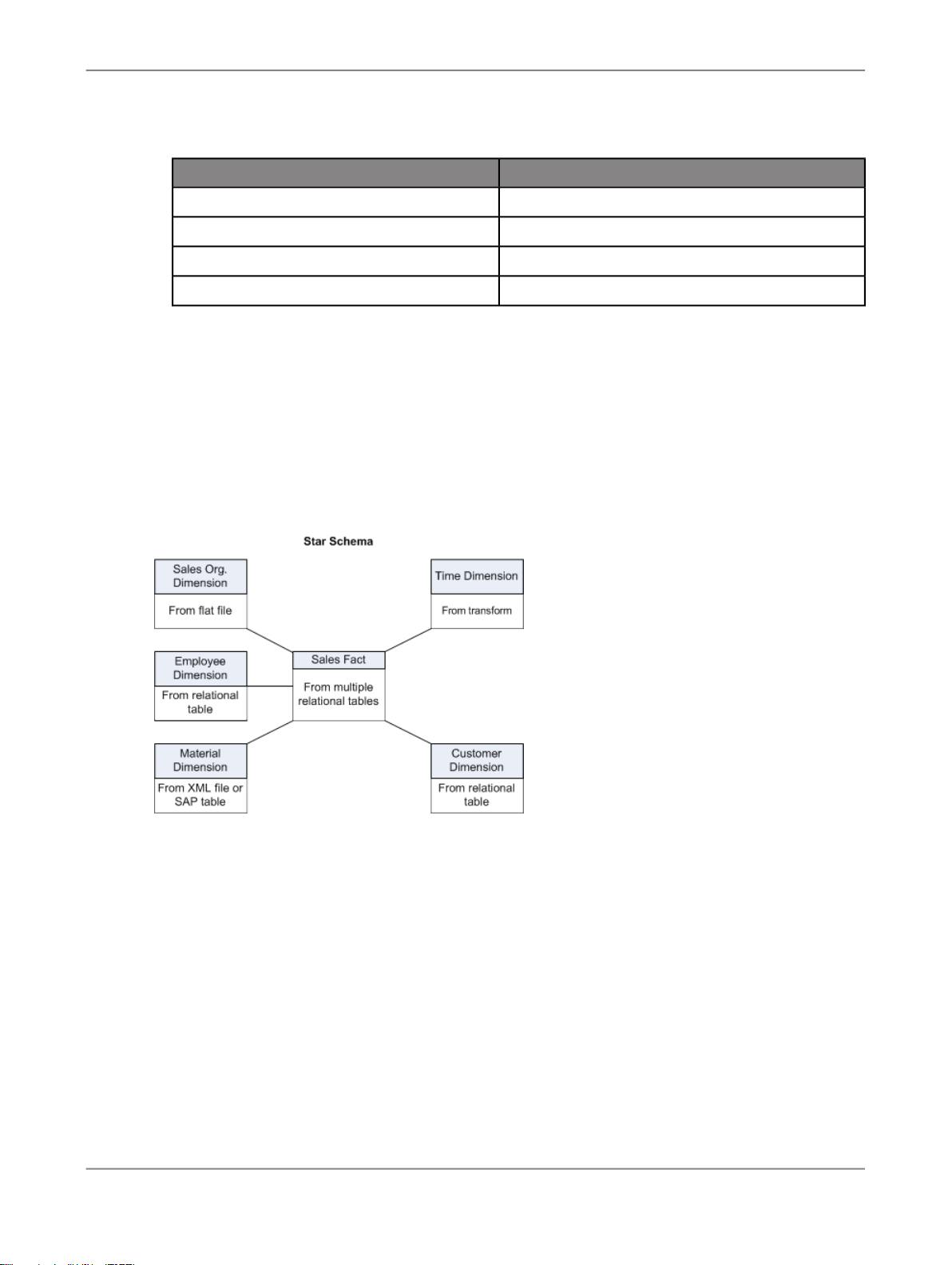
1.5 Tutorial structure
The goal of the tutorial exercises is to demonstrate SAP BusinessObjects Data Services features using
a simplified data model. The model is a sales data warehouse with a star schema that contains one
fact table and some dimension tables.
Table name in databaseDescriptive name
employee_dimEmployee Dimension
sales_factSales Fact
status_tableRecovery Status
CDC_timeCDC Status
Sections build on jobs you create and skills learned in previous sections. You must complete each
exercise to begin the next.
Note:
The screens in this guide are for illustrative purposes. On some screens, the available options depend
on the database type and version in the environment.
This tutorial is organized as follows.
Product Overview
Defining Source and Target Metadata
introduces the basic architecture and the user interface for Data Services.
introduces working with the Designer. Use the Designer to define
a datastore and a file format, then import metadata to the object library. After completing this section,
you will have completed the preliminary work required to define data movement specifications for flat-file
data.
2010-12-0219
Page 20

Introduction
Populating the SalesOrg Dimension from a Flat File
source and target tables. The exercise populates the sales organization dimension table from flat-file
data.
Populating the Time Dimension Using a Transform
creates a data flow for populating the time dimension table.
Populating the Customer Dimension from a Relational Table
tables. This exercise defines a job that populates the customer dimension table.
Populating the Material Dimension from an XML File
This exercise defines a job that populates the material dimension table.
Populating the Sales Fact Table from Multiple Relational Tables
tables and introduces joins and the lookup function. The exercise populates the sales fact table.
Changed-Data Capture
variables, parameters, functions, and scripts.
Data Assessment
exercise uses profile statistics, the validation transform, and the audit data flow feature.
Recovery Mechanisms
Multiuser Development
environment.
Extracting SAP Application Data
sources.
introduces a basic approach to changed-data capture. The exercise uses
introduces features to ensure and improve the validity of your source data. The
presents techniques for recovering from incomplete data loads.
presents the use of a central repository for setting up a multiuser development
provides optional exercises on extracting data from SAP application
introduces basic data flows, query transforms, and
introduces Data Services functions. This exercise
introduces data extraction from relational
introduces data extraction from nested sources.
continues data extraction from relational
Running a Real-time Job in Test Mode
mode.
1.6 Exiting the tutorial
You can exit the tutorial at any point after creating a sample project (see Adding a new project).
1.6.1 To exit the tutorial
1.
From the Project menu, click Exit.
If any work has not been saved, you are prompted to save your work.
2.
Click Yes or No.
provides optional exercises on running a real-time job in test
2010-12-0220
Page 21

Introduction
1.6.2 To resume the tutorial
1.
Log in to the Designer and select the repository in which you saved your work.
The Designer window opens.
2.
From the Project menu, click Open.
3.
Click the name of the project you want to work with, then click Open.
The Designer window opens with the project and the objects within it displayed in the project area.
2010-12-0221
Page 22

Introduction
2010-12-0222
Page 23

Product Overview
Product Overview
This section provides an overview of SAP BusinessObjects Data Services. It introduces the product
architecture and the Designer.
2.1 Product features
SAP BusinessObjects Data Services combines industry-leading data quality and integration into one
platform. With Data Services, your organization can transform and improve data anywhere. You can
have a single environment for development, runtime, management, security and data connectivity.
One of the fundamental capabilities of Data Services is extracting, transforming, and loading (ETL) data
from heterogeneous sources into a target database or data warehouse. You create applications (jobs)
that specify data mappings and transformations by using the Designer.
Use any type of data, including structured or unstructured data from databases or flat files to process
and cleanse and remove duplicate entries. You can create and deliver projects more quickly with a
single user interface and performance improvement with parallelization and grid computing.
Data Services RealTime interfaces provide additional support for real-time data movement and access.
Data Services RealTime reacts immediately to messages as they are sent, performing predefined
operations with message content. Data Services RealTime components provide services to web
applications and other client applications.
Data Services features
• Instant traceability with impact analysis and data lineage capabilities that include the data quality
process
• Data validation with dashboards and process auditing
• Work flow design with exception handling (Try/Catch) and Recovery features
• Multi-user support (check-in/check-out) and versioning via a central repository
• Administration tool with scheduling capabilities and monitoring/dashboards
• Transform management for defining best practices
• Comprehensive administration and reporting tools
• Scalable scripting language with a rich set of built-in functions
• Interoperability and flexibility with Web services-based applications
• High performance parallel transformations and grid computing
• Debugging and built-in profiling and viewing data
• Broad source and target support
2010-12-0223
Page 24

Product Overview
• applications (for example, SAP)
• databases with bulk loading and CDC changes data capture
• files: comma delimited, fixed width, COBOL, XML, Excel
For details about all the features in Data Services, see the
2.2 Product components
The Data Services product consists of several components including:
• Designer
The Designer allows you to create, test, and execute jobs that populate a data warehouse. It is a
development tool with a unique graphical user interface. It enables developers to create objects,
then drag, drop, and configure them by selecting icons in a source-to-target flow diagram. It allows
you to define data mappings, transformations, and control logic. Use the Designer to create
applications specifying work flows (job execution definitions) and data flows (data transformation
definitions).
• Job Server
The Job Server is an application that launches the Data Services processing engine and serves as
an interface to the engine and other components in the Data Services suite.
• Engine
The Data Services engine executes individual jobs defined in the application you create using the
Designer. When you start your application, the Data Services Job Server launches enough engines
to effectively accomplish the defined tasks.
Reference Guide.
• Repository
The repository is a database that stores Designer predefined system objects and user-defined
objects including source and target metadata and transformation rules. In addition to the local
repository used by the Designer and Job Server, you can optionally establish a central repository
for object sharing and version control.
The Designer handles all repository transactions. Direct manipulation of the repository is unnecessary
except for:
• Setup before installing Data Services
You must create space for a repository within your RDBMS before installing Data Services.
• Security administration
Data Services uses your security at the network and RDBMS levels.
• Backup and recovery
2010-12-0224
Page 25
Product Overview
• Access Server
• Administrator
You can export your repository to a file. Additionally, you should regularly back up the database
where the repository is stored.
The Access Server passes messages between web applications and the Data Services Job Server
and engines. It provides a reliable and scalable interface for request-response processing.
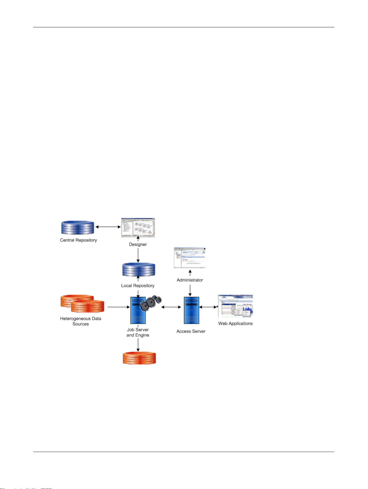
The Web Administrator provides browser-based administration of Data Services resources, including:
• Scheduling, monitoring, and executing batch jobs
• Configuring, starting, and stopping real-time services
• Configuring Job Server, Access Server, and repository usage
• Configuring and managing adapters
• Managing users
• Publishing batch jobs and real-time services via Web services
The following diagram illustrates Data Services product components and relationships.
2.3 Using the product
You use Data Services to design, produce, and run data movement applications.
2010-12-0225
Page 26
Product Overview
Using the Designer, you can build work flows and data flows that cleanse your data and specify data
extraction, transformation, and loading processes. In Data Services RealTime, you have the added
capability to build real-time data flows that support e-business transactions.
You create jobs to contain, organize, and run your flows. You create projects to organize the jobs.
Refine and build on your design until you have created a well-tested, production-quality application. In
Data Services, you can set applications to run in test mode or on a specific schedule. Using Data
Services RealTime, you can run applications in real time so they immediately respond to web-based
client requests.
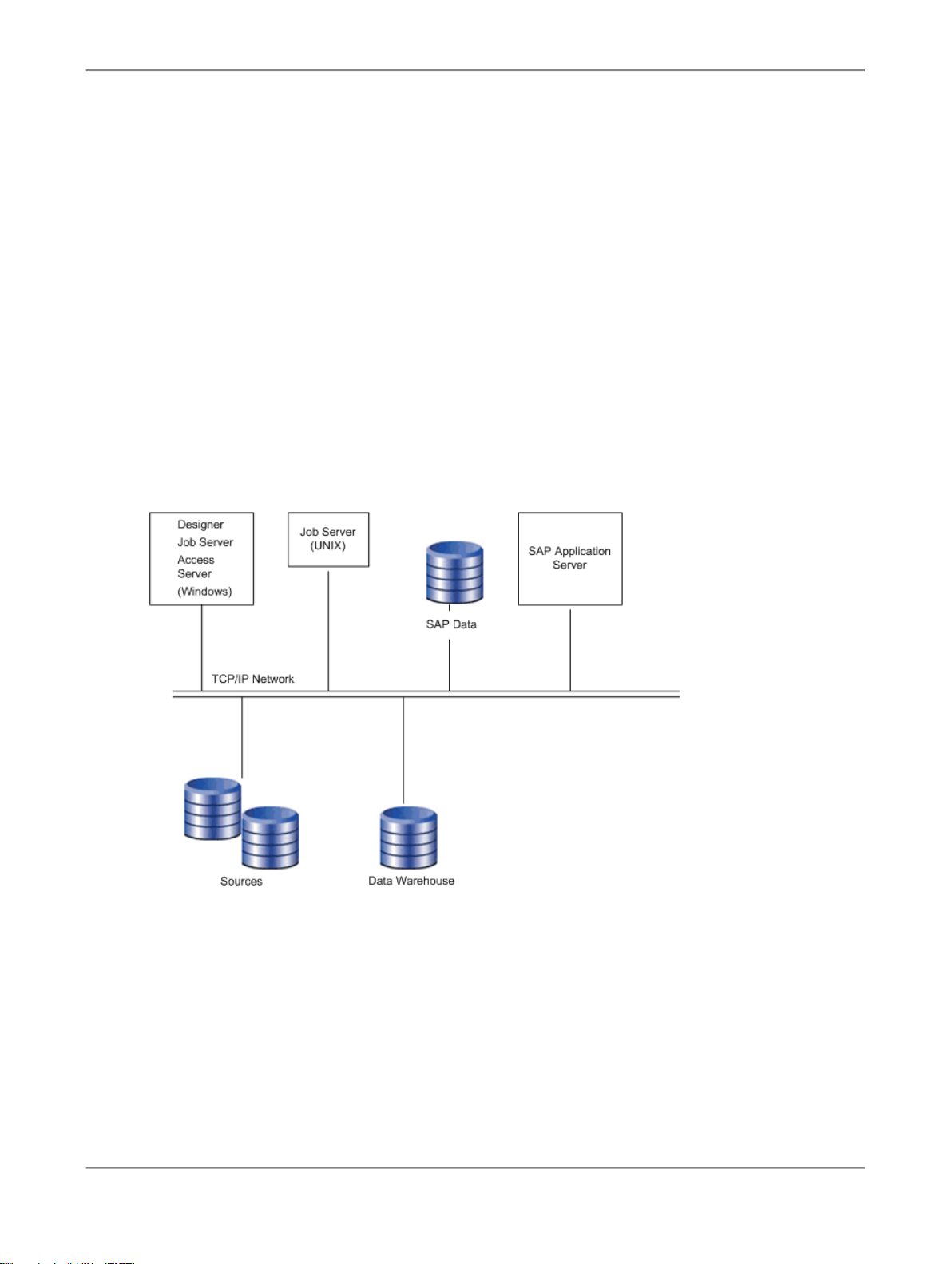
2.4 System configurations
You can configure SAP BusinessObjects Data Services in various ways. The following diagram illustrates
one possible system configuration.
When integrating Data Services into your existing environment, consider:
• The servers shown in the diagram can be separate physical computers, or they can be installed on
a single computer.
• For peak performance, install and create the Data Services local repository on either the same
computer as the Data Services Job Server or on the same computer as the target data warehouse.
In either of the previous configurations, the computer should be on the same LAN segment as the
rest of the Data Services components.
2010-12-0226
Page 27

Product Overview
As shown in the diagram, most Data Services components—the Designer, Job Server, and Access
Server—can run on the same Windows system, or you can install the Job Server on a UNIX system
running Hewlett Packard HP-UX, Sun Solaris, or IBM AIX.
2.4.1 Windows implementation
You can configure a Windows system as either a server or a workstation. A large-memory, multiprocessor
system is ideal because the multithreading, pipelining, and parallel work flow execution features in Data
Services take full advantage of such a system.
You can create your target data warehouse on a database server that may or may not be a separate
physical computer.
You can use a shared disk or FTP to transfer data between your source system and the Data Services
Job Server.
2.4.2 UNIX implementation
You can install the Data Services Job Server on a UNIX system. You can also configure the Job Server
to start automatically when you restart the computer.
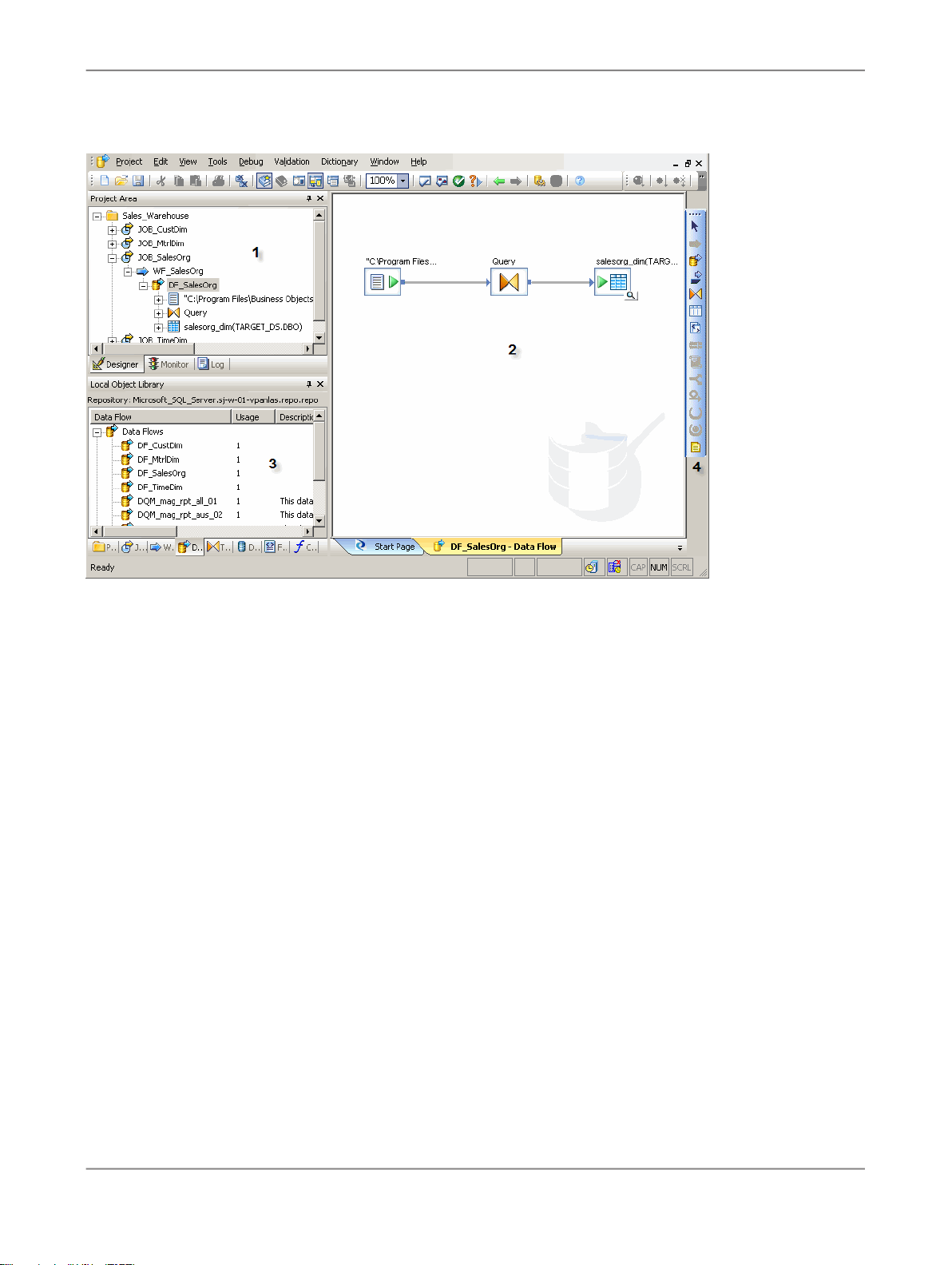
2.5 The Designer window
The following illustration shows the key areas of the Designer window.
2010-12-0227
Page 28
Product Overview
The key areas of the Data Services application window are:
1.
Project area — Contains the current project (and the job(s) and other objects within it) available to
you at a given time. In Data Services, all entities you create, modify, or work with are objects.
2.
Workspace — The area of the application window in which you define, display, and modify objects.
3.
Local object library — Provides access to local repository objects including built-in system objects,
such as transforms and transform configurations, and the objects you build and save, such as jobs
and data flows.
4.
Tool palette — Buttons on the tool palette enable you to add new objects to the workspace.
2.6 SAP BusinessObjects Data Services objects
In SAP BusinessObjects Data Services, all entities you add, define, modify, or work with are objects.
Objects have:
• Options that control the object. For example, to set up a connection to a database, defining the
database name would be an option for the connection.
• Properties that describe the object. For example, the name and creation date. Attributes are properties
used to locate and organize objects.
2010-12-0228
Page 29

Product Overview
• Classes that determine how you create and retrieve the object. You can copy reusable objects from
The following diagram shows transform objects in the Data Services object library.
the object library. You cannot copy single-use objects.
When you widen the object library, the name of each object is visible next to its icon. To resize the
object library area, click and drag its border until you see the text you want, then release.
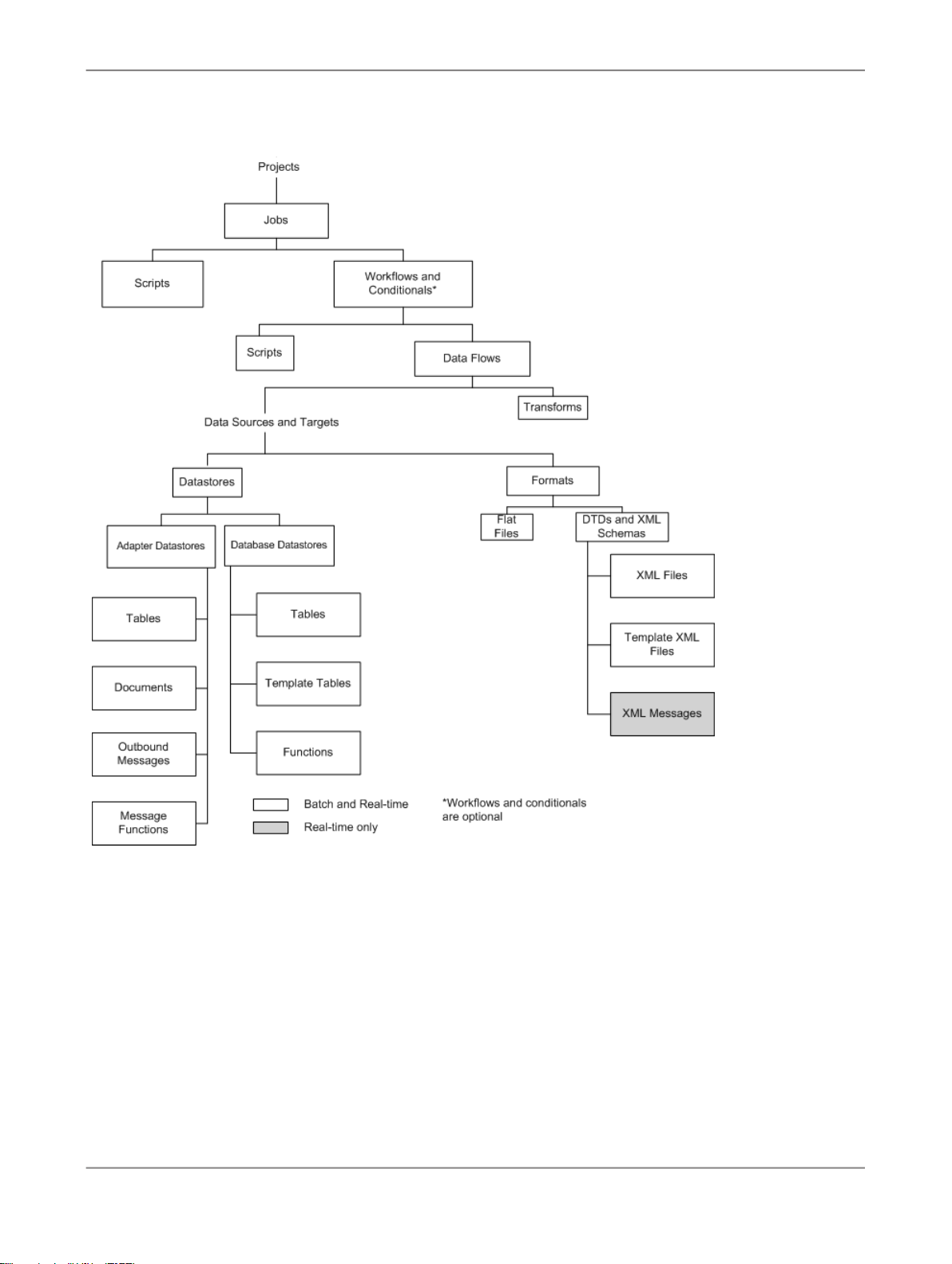
2.6.1 Object hierarchy
The following illustration shows the hierarchical relationships for the key object types within Data
Services.
2010-12-0229
Page 30
Product Overview
In the repository, the Designer groups objects hierarchically from a project, to jobs, to optional work
flows, to data flows. In jobs:
• Work flows define a sequence of processing steps. Work flows and conditionals are optional. A
conditional contains work flows, and you can embed a work flow within another work flow.
• Data flows transform data from source(s) to target(s). You can embed a data flow within a work flow
or within another data flow.
2010-12-0230
Page 31

Product Overview
2.6.1.1 Projects and jobs
A project is the highest-level object in the Designer window. Projects provide you with a way to organize
the other objects you create in Data Services. Only one project is open at a time (where "open" means
"visible in the project area").
A “job” is the smallest unit of work that you can schedule independently for execution.
2.6.1.2 Work flows and data flows
Jobs are composed of work flows and/or data flows:
• A “work flow” is the incorporation of several data flows into a coherent flow of work for an entire job.
• A “data flow” is the process by which source data is transformed into target data.
A work flow orders data flows and operations that support them; a work flow also defines the
interdependencies between data flows. For example, if one target table depends on values from other
tables, use the work flow to specify the order in which you want Data Services to populate the tables.
Also use work flows to define strategies for handling errors that occur during project execution. You
can also use work flows to define conditions for running sections of a project.
The following diagram illustrates a typical work flow.
A data flow defines the basic task that Data Services accomplishes, which involves moving data from
one or more sources to one or more target tables or files. You define data flows by identifying the
sources from which to extract data, the transformations that the data should undergo, and targets.
2010-12-0231
Page 32

Product Overview
Blueprints
We have identified a number of common scenarios that you are likely to handle with Data Services.
Instead of creating your own job from scratch, look through the blueprints. If you find one that is closely
related to your particular business problem, you can simply use the blueprint and tweak the settings in
the transforms for your specific needs.
For each scenario, we have included a blueprint that is already set up to solve the business problem
in that scenario. Each blueprint contains the necessary Data Services project, jobs, data flows, file
formats, sample data, template tables, and custom functions to run the data flows in your environment
with only a few modifications.
You can download all of the blueprints or only the blueprints and other content that you find useful from
the SAP BusinessObjects Community Network. Here, we periodically post new and updated blueprints,
custom functions, best practices, white papers, and other Data Services content. You can refer to this
site frequently for updated content and use the forums to provide us with any questions or requests
you may have. We have also provided the ability for you to upload and share any content that you have
developed with the rest of the Data Services development community.
Instructions for downloading and installing the content objects are also located on the SAP
BusinessObjects Community Network at http://www.sdn.sap.com/irj/boc/blueprints.
2.6.2 Object-naming conventions
Data Services recommends that you follow a consistent naming convention to facilitate object
identification. Here are some examples:
2.7 New terms
ExampleObjectSuffixPrefix
JOB_SalesOrgJobJOB
WF_SalesOrgWork flowWF
DF_CurrencyData flowDF
ODS_DSDatastoreDS
2010-12-0232
Page 33

Product Overview
DescriptionTerm
Property that can be used as a constraint for locating objects.Attribute
Data flow
Job
Object
Object library
Contains steps to define how source data becomes target data. Called by a work
flow or job.
Logical channel that connects Data Services to source and target databases.Datastore
The smallest unit of work that you can schedule independently for execution. A job
is a special work flow that cannot be called by another work flow or job.
Data that describes the objects maintained by Data Services.Metadata
Any project, job, work flow, data flow, datastore, file format, message, custom function,
transform, or transform configurations created, modified, or used in Data Services.
Part of the Designer interface that represents a "window" into the local repository
and provides access to reusable objects.
A choice in a dialog box that controls how an object functions.Option
Logical grouping of related jobs. The Designer can open only one project at a time.Project
Property
Repository
Work flow
Characteristic used to define the state, appearance, or value of an object; for example,
the name of the object or the date it was created.
A database that stores Designer predefined system objects and user-defined objects
including source and target metadata and transformation rules. Can be local or
central (shared).
Table, file, or legacy system from which Data Services reads data.Source
Table or file to which Data Services loads data.Target
Contains steps to define the order of job execution. Calls a data flow to manipulate
data.
2010-12-0233
Page 34

Product Overview
2.8 Section summary and what to do next
This section has given you a short overview of the Data Services product and terminology. For more
information about these topics, see the
Administrator Guide
and the
Designer Guide
.
2010-12-0234
Page 35

Defining Source and Target Metadata
Defining Source and Target Metadata
In this section you will set up logical connections between Data Services, a flat-file source, and a target
data warehouse. You will also create and import objects into the local repository. Storing connection
metadata in the repository enables you to work within Data Services to manage tables that are stored
in various environments.
3.1 Logging in to the Designer
When you log in to the Designer, you must log in as a user defined in the Central Management Server
(CMS).
1.
From the Start menu, click Programs > SAP BusinessObjects Data Services XI 4.0 > Data
Services Designer.
As Data Services starts, a login screen appears.
2.
Enter your user credentials for the CMS.
• System
Specify the server name and optionally the port for the CMS.
• User name
Specify the user name to use to log into CMS.
• Password
Specify the password to use to log into the CMS.
• Authentication
Specify the authentication type used by the CMS.
3.
Click Log On.
The software attempts to connect to the CMS using the specified information. When you log in
successfully, the list of local repositories that are available to you is displayed.
4.
Select the repository you want to use.
5.
Click OK to log in using the selected repository.
In the next section you will define datastores (connections) for your source and target.
2010-12-0235
Page 36

Defining Source and Target Metadata
3.2 Defining a datastore
Datastores:
• Provide a logical channel (connection) to a database
• Must be specified for each source and target database
• Are used to import metadata for source and target databases into the repository.
• Are used by Data Services to read data from source tables and load data to target tables
The databases to which Data Services datastores can connect include:
• Oracle
• IBM DB2
• Microsoft SQL Server
• Sybase ASE
• Sybase IQ
• ODBC
Metadata consists of:
• Database tables
• Table name
• Column names
• Column data types
• Primary key columns
• Table attributes
• RDBMS functions
• Application-specific data structures
Connection metadata is defined in the object library as datastores (for tables) and file formats (for flat
files).
The next task describes how to define datastores using the Designer. Note that while you are designating
the datastores as sources or targets, datastores only function as connections. You will define the actual
source and target objects when you define data flows later in the tutorial.
3.2.1 To define a datastore for the source (ODS) database
1.
From the Datastores tab of the object library, right-click in the blank area and click New.
The "Create New Datastore" window opens. A example for the Oracle environment appears as
follows:
2010-12-0236
Page 37

Defining Source and Target Metadata
2.
In the Datastore name box, type ODS_DS.
This datastore name labels the connection to the database you will use as a source. The datastore
name will appear in the local repository. When you create your own projects/applications, remember
to give your objects meaningful names.
3.
In the Datastore type box, click Database.
4.
In the Database type box, click the option that corresponds to the database software being used
to store the source data.
The remainder of the boxes on the "Create New Datastore" window depend on the Database type
you selected.
The following table lists the minimum options to configure for some common Database types. Enter
the information you recorded in Create repository, source, and target databases on an existing
RDBMS.
Sybase ASEMS SQL ServerDB2Oracle
Database versionEnable CDCEnable CDCEnable CDC
Database server nameDatabase versionDatabase versionDatabase version
Database nameDatabase server nameData sourceConnection name
User nameDatabase nameUser nameUser name
PasswordUser namePasswordPassword
Password
5.
Click OK.
Data Services saves a datastore for your source in the repository.
2010-12-0237
Page 38

Defining Source and Target Metadata
3.2.2 To define a datastore for the target database
Define a datastore for the target database using the same procedure as for the source (ODS) database.
1.
Use Target_DS for the datastore name.
2.
Use the information you recorded in Create repository, source, and target databases on an existing
RDBMS.
3.3 Importing metadata
With Data Services, you can import metadata for individual tables using a datastore. You can import
metadata by:
• Browsing
• Name
• Searching
The following procedure describes how to import by browsing.
3.3.1 To import metadata for ODS source tables
1.
In the Datastores tab, right-click the ODS_DS datastore and click Open.
The names of all the tables in the database defined by the datastore named ODS_DS display in a
window in the workspace.
2.
Move the cursor over the right edge of the Metadata column heading until it changes to a resize
cursor.
3.
Double-click the column separator to automatically resize the column.
4.
Import the following tables by right-clicking each table name and clicking Import. Alternatively,
because the tables are grouped together, click the first name, Shift-click the last, and import them
together. (Use Ctrl-click for nonconsecutive entries.)
• ods.ods_customer
• ods.ods_material
• ods.ods_salesorder
• ods.ods_salesitem
• ods.ods_delivery
2010-12-0238
Page 39

Defining Source and Target Metadata
• ods.ods_employee
• ods.ods_region
Data Services imports the metadata for each table into the local repository.
Note:
In Microsoft SQL Server, the owner prefix might be dbo instead of ods.
5.
In the object library on the Datastores tab, under ODS_DS expand the Tables node and verify the
tables have been imported into the repository.
3.3.2 To import metadata for target tables
1.
Open the Target_DS datastore.
2.
Import the following tables by right-clicking each table name and clicking Import. Alternatively, use
Ctrl-click and import them together
• target.status_table
• target.cust_dim
• target.employee_dim
• target.mtrl_dim
• target.sales_fact
• target.salesorg_dim
• target.time_dim
• target.CDC_time
Data Services imports the metadata for each table into the local repository.
Note:
In Microsoft SQL Server, the owner prefix might be dbo instead of target.
3.
In the object library on the Datastores tab, under Target_DS expand the Tables node and verify
the tables have been imported into the repository.
3.4 Defining a file format
If the source or target RDBMS includes data stored in flat files, you must define file formats in Data
Services. File formats are a set of properties that describe the structure of a flat file.
Data Services includes a file format editor. Use it to define flat file formats. The editor supports delimited
and fixed-width formats.
2010-12-0239
Page 40

Defining Source and Target Metadata
You can specify file formats for one file or a group of files. You can define flat files from scratch or by
importing and modifying an existing flat file. Either way, Data Services saves a connection to the file or
file group.
Note:
Data Services also includes a file format (Transport_Format) that you can use to read flat files in SAP
applications.
In the next section, you will use a flat file as your source data. Therefore, you must create a file format
and connection to the file now.
3.4.1 To define a file format
1.
In the object library, click the Formats tab, right-click in a blank area of the object library, and click
New > File Format.
The file format editor opens.
2.
Under General, leave Type as Delimited. Change the Name to Format_SalesOrg.
3.
Under Data File(s), beside File name(s), click the Files folder icon and navigate in your Data Services
install directory to %LINK_DIR%\Tutorial Files\sales_org.txt. Click Open.
Note:
The file format editor initially displays default values for the file schema. When you select a file, a
prompt asks you to verify that you want to overwrite the current schema with the schema from the
file you selected. Click Yes.
The file format editor displays sample data from the sales_org.txt file in the (lower right) Data Preview
pane.
4.
Under Default Format, change Date to ddmmyyyy.
The source data contains dates with a two-digit day number followed by a two-digit month number,
a four-digit year (ddmmyyyy), and no time value. (Note that the sample dates do not contain a
delimiter between values. Using an unsupported format string such as ddmmJJJJ will result in
incorrect dates, and no error message will appear.)
5.
The first row contains the names of the column headings. Under Input/Output, change Skip row
header to Yes.
Data Services removes the first row and uses these column heading values for the field names in
the upper-right Column Attributes pane.
Note:
A prompt asks you to verify that you want to overwrite the current schema with the schema (column
headings) from the file you selected. Click Yes.
6.
In the upper-right Column Attributes pane, click DateOpen and change the data type to Date.
The column types and lengths should appear as follows:
2010-12-0240
Page 41

Defining Source and Target Metadata
Field SizeData TypeField Name
IntSalesOffice
2VarCharRegion
DateDateOpen
7VarCharCountry
7.
Click Save & Close.
3.5 New terms
The terms examined in this section included:
Datastore
MeaningTerm
Connection from Data Services to tables in source or target databases. Stored as an
object in the repository.
2010-12-0241
Page 42

Defining Source and Target Metadata
MeaningTerm
Data that describes objects maintained by Data Services. Metadata that Data Services
stores in its local repository includes:
• Table name
• Column name
Metadata
• Column data types
• Primary key columns
• Table attributes
• RDBMS functions
The GUI part of the Designer representing the local repository.Object library
File format
A set of properties that define the table structure for a flat file. Stored as an object in
the repository.
3.6 Summary and what to do next
At this point, you have finished all the preparatory work to define data movement specifications for a
flat-file data source to a target data warehouse. In this section you have:
• Defined a datastore from Data Services to your target data warehouse
• Imported metadata from target tables into the local repository so that you can use the Designer to
work with these tables
• Defined file formats and a connection to flat-file source data
You are now ready to create a new project and define jobs that will populate the target tables with
source data. You will do that for the sales organization dimension table in the next section.
You can now exit Data Services or go on to the next section. The information you have created in this
section has been saved in the local repository and will be automatically available to you the next time
you use Data Services.
For more information about the topics in this section, see the
Designer Guide
.
2010-12-0242
Page 43

Populating the SalesOrg Dimension from a Flat File
Populating the SalesOrg Dimension from a Flat File
In this section, you will populate the sales organization dimension table in your target data warehouse
with data from a flat file called Format_SalesOrg.
4.1 Objects and their hierarchical relationships
Everything in Data Services is an object. The key objects involved in data movement activities (like
projects, jobs, work flows, and data flows) display in the Designer project area according to their
relationship in the object hierarchy.
The following figure shows a display of the types of objects you will be creating while you are working
in this section.
1.
Project
2010-12-0243
Page 44

Populating the SalesOrg Dimension from a Flat File
2.
Job
3.
Work flow
4.
Data flow
Object hierarchies are displayed in the project area of the Designer.
4.2 Adding a new project
Projects group and organize related objects. Projects display in the project area of the Designer and
can contain any number of jobs, work flows, and data flows.
4.2.1 To add a new project
1.
In the Designer, from the Project menu click New > Project.
2.
Name the project Class_Exercises.
3.
Click Create.
The project name appears as the only object in the project area of the Designer.
Next, you will define the job that will be used to extract the information from the flat-file source.
4.3 Adding a job
A job is a reusable object. It is also the second level in the project hierarchy. It contains work flows
(which contain the order of steps to be executed) and data flows (which contain data movement
instructions). You can execute jobs manually or as scheduled.
In this exercise you will define a job called JOB_SalesOrg.
4.3.1 To add a new batch job
1.
Right-click in the project area and click New Batch Job.
2010-12-0244
Page 45

Populating the SalesOrg Dimension from a Flat File
2.
Right-click the new job and click Rename. Alternatively, left-click the job twice (slowly) to make the
name editable.
3.
Type JOB_SalesOrg.
4.
Left-click or press Enter.
The job appears in the project hierarchy under Class_Exercises and in the project tab of the object
library.
4.4 Adding a work flow
A work flow is a reusable object. It executes only within a Job. Use work flows to:
• Call data flows
• Call another work flow
• Define the order of steps to be executed in your job
• Pass parameters to and from data flows
• Define conditions for executing sections of the project
• Specify how to handle errors that occur during execution
Work flows are optional.
The Data Services objects you can use to create work flows appear on the tool palette:
Programming AnalogyComponentButton
ProcedureWork flow
Data Flow
Declarative SQL select statement
Subset of lines in a procedureScript
If/then/else logicConditional
A sequence of steps that re-
While Loop
peats as long as a condition is
true
2010-12-0245
Page 46

Populating the SalesOrg Dimension from a Flat File
Programming AnalogyComponentButton
Try block indicatorTry
4.4.1 To add a work flow
1.
With JOB_SalesOrg selected in the project area, click the work flow button on the tool palette.
2.
Click the blank workspace area.
A work flow icon appears in the workspace. The work flow also appears in the project area on the
left under the job name (expand the job to view).
Note:
You can place a work flow anywhere in the workspace, but because flows are best viewed from left
to right and top to bottom, place it near the top left corner.
Catch
Annotation
Try block terminator and exception handler
Description of a job, work flow,
data flow, or a diagram in a
workspace
3.
Change the name of the work flow to WF_SalesOrg.
4.
Click the name of the work flow.
2010-12-0246
Page 47

Populating the SalesOrg Dimension from a Flat File
An empty view for the work flow appears in the workspace. You will use this view to define the
elements of the work flow. Notice the title bar changes to display the name of the work flow.
4.5 About data flows
A data flow defines the flow of data from sources to targets. It is used to:
• Identify the source data that you want to read
• Define the transformations that you want to perform on the data
• Identify the target table to which you want to load data
A data flow is a reusable object. It is always called from a work flow or a job.
The first data flow you need to create for this tutorial reads sales organization data from a flat file and
loads the data into the sales organization dimension table in the target data warehouse.
4.5.1 Adding a data flow
The following procedure creates a data flow named DF_SalesOrg inside the work flow WF_SalesOrg.
4.5.1.1 To add a data flow
1.
Make sure the work flow window is open in the workspace.
If it is not, click the WF_SalesOrg work flow in the project area.
2.
Click the data flow button on the tool palette.
3.
Click the workspace.
A representation of a data flow appears in the workspace. The data flow also appears in the project
area.
4.
Change the name of the data flow to DF_SalesOrg.
Notice the project, job, work flow, and data flow objects display in hierarchical form in both the project
area and the object library. To navigate to these levels, click their names in the project area.
2010-12-0247
Page 48

Populating the SalesOrg Dimension from a Flat File
1—Data flow in the workspace
2—Data flow in the project area
3—Data flow in the local object library
5.
Click the data flow name.
A definition area for the data flow appears in the workspace. This area will be used to define the
data flow as described in the next section.
4.5.2 Defining the data flow
Inside the data flow, you must specify the instructions to transform source data into the form you want
for the target table. In this case, you will define the data flow instructions for building the sales organization
dimension table using the following objects:
• An object representing the source file
2010-12-0248
Page 49

Populating the SalesOrg Dimension from a Flat File
• An object defining a query transform (or query). A query transform maps columns from source to
target. With a query transform, you can:
• Select row sets
• Create joins
• Group and order by data values
• Create data set filters
• Execute functions
• An object representing the target table into which the data loads
The next three exercises guide you through the steps necessary to define a data flow's content:
1.
Add objects to the data flow.
2.
Connect them in the order that data will flow through them.
3.
Define the query that maps the source columns to the target columns.
4.5.2.1 To add objects to a data flow
1.
Verify the DF_SalesOrg data flow is open in the workspace. In the object library, click the Formats
tab.
2.
The source for this data flow will be the flat file Format_SalesOrg. Click and drag the Format_SalesOrg
object to the workspace.
3.
Drop the Format_SalesOrg object on the left side of the workspace to leave room for more objects
on the right.
4.
Click Make Source from the shortcut menu that appears when you drop the object.
5.
Click the query button on the tool palette.
6.
Click to the right of the source file in the workspace.
7.
In the object library, click the Datastores tab and expand the datastore named Target_DS.
8.
The target for this data flow will be the table SALESORG_DIM. Click and drag the SALESORG_DIM
object to the workspace and drop it to the right of the query.
9.
Click Make Target from the shortcut menu that appears when you drop the table. Data Services
creates a table with the same schema as the query output schema.
All the elements necessary to create the sales organization dimension table are now in the workspace.
In the next section, you will connect the steps in the correct order.
4.5.2.2 To define the order of steps in a data flow
You now need to define the sequence for the data flow. The steps execute in left-to-right order.
2010-12-0249
Page 50

Populating the SalesOrg Dimension from a Flat File
1.
Click the square on the right edge of the source file and drag it to the triangle on the left edge of the
query transform.
2.
Use the same drag technique to connect the query transform to the target table.
The next section introduces the query transform and the query transform editor.
4.5.2.3 To define a query transform that maps a source to a target
1.
Click the name of the query in the project area or in the workspace.
The query editor opens showing the source schema, the target schema (which has automatically
been copied from the target table metadata to the output pane of the query), and options for defining
the query.
There are four columns in the source schema: SalesOffice, Region, DateOpen, and Country. You
will specify that three of them (SalesOffice, Region, and DateOpen) be copied to the target table.
2.
Map the source columns to target columns by dragging and dropping each source column name
onto the corresponding column for the target schema. Notice that the column icon next to the source
column changes to an arrow when dragged to the target, which indicates that the column has been
mapped.
Also notice that when you select a column in the target schema, the Mapping tab in the query options
shows the mapping relationship for that column. You can also view the mapping relationship by
scrolling the Schema Out pane to the right to show the Mapping column.
2010-12-0250
Page 51

Populating the SalesOrg Dimension from a Flat File
a.
Target schema
b.
Source schema
c.
Query options
d.
Column mapping definition
3.
Validate the query by clicking the Validate Current button on the toolbar.
The Output window appears with tabs for Errors, Warnings, and Information. The Warning tab
indicates that Data Services will convert the data type for the SALESOFFICE column.
4.
Close the Output window and click the Back arrow on the tool bar to close the query editor and
return to the data flow view.
4.5.3 Validating the data flow
Next you will verify that the data flow has been constructed properly (which does not guarantee that
the job will run or produce the correct data).
The Validation menu provides design-time validation options. These options check for syntax errors,
not run-time errors. Run-time validation occurs while the job executes.
4.5.3.1 To validate a data flow
1.
Click DF_SalesOrg in the project area.
2.
From the menu bar, click Validation > Validate > Current View.
Note:
• Current View —Validates the object definition open in the workspace.
• All Objects in View — Validates the object definition open in the workspace and all of the objects
that it calls.
2010-12-0251
Page 52

Populating the SalesOrg Dimension from a Flat File
Also note the Validate Current and Validate All buttons on the toolbar. These buttons perform the
same validation as Current View and All Objects in View, respectively.
Data Services displays the "Output" dialog box with the Warning tab indicating that Data Services will
convert the data type for the SALESOFFICE column.
If the "Output" window displays any errors, correct them before proceeding.
4.5.4 Addressing errors
4.5.4.1 To use the Output window
1.
Right-click an error message and click View.
Data Services displays the "Error Message" window in which you can read the expanded error
message text.
2.
Double-click the error message to open the editor of the object containing the error.
Note:
Warning messages do not prohibit job execution.
You have validated the data flow and completed the description of the data movement for the sales
organization dimension table.
4.6 Saving the project
You can save the steps you have completed and close Data Services at any time.
To save all objects in a project, from the Project menu click Save All. Or, when you close a project or
exit the program, Data Services lists all recently changed items and prompts you to save them.
To save work displayed only in the active object workspace, from the Project menu click Save.
2010-12-0252
Page 53

Populating the SalesOrg Dimension from a Flat File
4.7 To execute the job
Now you will execute the job you have just created.
First verify that your job server is running by looking at the job server icon at the bottom right of the
Designer window. Move the pointer over the icon to see the Job Server name, machine name, and port
number in the status area. If the job server is not running, the icon will have a red X on it.
1.
Select the job name in the project area, in this case JOB_SalesOrg.
2.
Right-click and click Execute.
If you have changed any objects and not yet saved them, Data Services prompts you to save your
work. Click OK.
Data Services validates the job again before running it. If there are syntax errors, review the error
messages and return to the design and validate the effected steps of the job. Also review any warning
messages before dismissing them.
If the job validates properly, the "Execution Properties" dialog box appears. These properties include
execution parameters and options to set traces and global variables.
2010-12-0253
Page 54

Populating the SalesOrg Dimension from a Flat File
To set or change a job's default execution settings, right-click the job name and click Properties.
3.
For this exercise, do not change the defaults. Click OK.
Data Services executes the job and produces three log files:
• Trace log: A list of the job steps in the order they started.
• Monitor log: A list of each step in the job, the number of rows processed by that step, and the
time required to complete the operation.
• Error log: A list of any errors produced by the RDBMS, Data Services, or the computer operating
system during the job execution.
The log window opens in the workspace and displays the trace log. The buttons at the top of the log
window show which kind of log you are viewing. Clicking the middle button displays the monitor log,
and the right-hand button shows the error log.
2010-12-0254
Page 55

Populating the SalesOrg Dimension from a Flat File
4.
Use the buttons at the top of the log window to view the monitor log. Because there are no errors
or warnings, the error log button is unavailable (there is no error log to examine).
5.
After the job is complete, use your RDBMS query tool to check the contents of the table named
salesorg_dim.
4.8 About deleting objects
Deleting a job or other object from the project area does not delete it from the object library. The object
still exists in any other projects to which it has been assigned. Deleting an object from the object library,
however, deletes all occurrences of the object.
4.9 New terms
The terms introduced in this section included:
2010-12-0255
Page 56

Populating the SalesOrg Dimension from a Flat File
MeaningTerm
Query options
Transform
4.10 Summary and what to do next
You have now defined and run your first data movement job—a job that populates the sales organization
dimension table in the target data warehouse.
The next section introduces you to time dimension tables. In that exercise you will populate the time
dimension table with some simple time attributes:
• Year number
Tabs in the query editor that defines properties
of the output schema
A Data Services transform objectQuery
A description of the data layout of a tableSchema
A Data Services object that defines data transformation
• Month number
• Business quarter
The next section also introduces you to the Date_Generation transform.
2010-12-0256
Page 57

Populating the Time Dimension Using a Transform
Populating the Time Dimension Using a Transform
The exercise in this section builds and populates a time dimension table. Time dimension tables contain
date/time-related attributes such as season, holiday period, fiscal quarter, and others that are not directly
ascertainable from traditional SQL style date/time data types.
The time dimension table in this example is simple in that it contains only the year number, month
number, and business quarter as time attributes. It uses a Julian date as a primary key.
The tasks in this section include:
• Retrieving the project
• Adding the job and data flow
• Defining the time dimension data flow
• Saving and executing the job
5.1 Retrieving the project
If you have closed Data Services, reopen the Class_Exercises project.
2010-12-0257
Page 58

Populating the Time Dimension Using a Transform
5.1.1 To open the Class_Exercises project
1.
Start Data Services.
2.
Log in to your repository.
3.
Click Project > Open.
4.
Click Class_Exercises.
5.
Click OK.
5.2 Adding the job and data flow
As you have done in the previous exercise, you will begin with creating a job that contains a data flow.
A work flow is not necessary for this job; you will be calling the data flow directly from the job.
5.2.1 To add the job and data flow
1.
Add a job named JOB_TimeDim that will load data into the time dimension table.
For a reminder about how to create a job, see Adding a job.
2.
Open JOB_TimeDim and create a data flow object named DF_TimeDim. (Do not create a work flow
this time.)
5.3 Defining the time dimension data flow
The data flow instructions for populating a time dimension table consist of the following objects:
• A Date_Generation transform as a source.
• A query to produce column values from the generated dates such as what day the date falls on, the
quarter it's in, and so on.
• A target table into which the time dimension data loads.
2010-12-0258
Page 59

Populating the Time Dimension Using a Transform
5.3.1 To specify the components of the time data flow
1.
Open the data flow named DF_TimeDim.
2.
In the object library, click the Transforms tab.
3.
Expand the Data Integrator folder and click the Date_Generation transform.
Transforms are predefined Data Services objects.
4.
Drag the transform icon into the workspace and drop it on the left side of the workspace to leave
room for more objects to the right.
5.
Click the query button on the tool palette.
6.
Click in the workspace to the right of the Date_Generation transform.
7.
In the object library for the datastore named Target_DS, drag the table named TIME_DIM into the
workspace and drop it to the right of the query.
8.
Click Make Target from the shortcut menu.
All the objects you need to create a time dimension table are now available in the workspace. Next you
will connect the objects in the order they need to be executed.
5.3.2 To define the flow of data
1.
Click the square on the right edge of the Date_Generation transform and drag to the triangle on the
left edge of the query.
2.
Use the same drag technique to connect the query to the TIME_DIM target.
The connections indicate the flow of data through these instructions.
The following sections define the details of each step of the data flow.
5.3.3 To define the output of the Date_Generation transform
2010-12-0259
Page 60

Populating the Time Dimension Using a Transform
The Date_Generation transform produces a column of dates for a range and increment you specify.
1.
Click the name of the Date_Generation transform to open the transform editor.
2.
Enter these values in the editor columns:
Start Date
End Date
Increment
3.
Click the Back arrow in the tool bar to close the transform editor and return to the data flow.
The date column serves as the input to the query. The query allows you to apply functions to the input
columns and map those columns to an internal data set (the query output).
5.3.4 To define the output of the query
1.
Click the query icon in the project area.
The query editor shows an input schema with a single column, the output schema copied from the
target, and options for the query.
2.
Map the generated date to the NATIVEDATE column by dragging the DI_GENERATED_DATE
column from the input schema to the NATIVEDATE output column.
2002.01.01
2008.12.31
daily
2010-12-0260
Page 61

Populating the Time Dimension Using a Transform
Alternatively, you can drag and drop the DI_GENERATED_DATE column from the source pane into
the mapping expression. The column name DI_GENERATED_DATE will be qualified with the name
of the Date_Generation transform; for example, Date_Generation_1.DI_GENERATED_DATE.
3.
Click each column name in the target schema (one by one) and define the mapping for the column
using the following table. The mapping definition applies to the column selected in the target schema.
Type the mapping expression directly on the Mapping tab.
Alternatively, click the Functions button to open the Function editor and add functions to the mapping
definition that way.
These are the mapping expressions and function descriptions for the rest of the columns:
Function descriptionMappingColumn name
Use the JULIAN function to set
the Julian date for that date
value.
Date_ID
julian(di_generat
ed_date)
Use the TO_CHAR function to
YearNum
to_char(di_generat
ed_date,'yyyy')
select only the year out of the
date value. Enclose yyyy in
single quotes.
Use the MONTH function to set
the month number for that date
value.
Use the QUARTER function to
set the quarter for that date
value.
MonthNum
BusQuarter
month(di_generat
ed_date)
quarter(di_generat
ed_date)
You might notice that the tutorial simplifies the quarter calculation. For the purposes of the tutorial,
assume that the business year is the same as the calendar year.
4.
Click the Back arrow on the tool bar.
2010-12-0261
Page 62

Populating the Time Dimension Using a Transform
These columns are now the input schema for the TIME_DIM table.
This completes the data-movement description for the time dimension table.
5.4 Saving and executing the job
Save the project. For a reminder of how to save a project, see Saving the project.
Execute the job JOB_TimeDim. After the job runs, check the contents of the TIME_DIM table with a
query tool for the RDBMS on which your target data warehouse is stored.
5.5 Summary and what to do next
You have now populated two tables in the sales data warehouse:
• Sales Org dimension (from a flat file)
• Time dimension, which consists of a date generation transform and a query
In the next section, you will extract data to populate the customer dimension table.
At this point, you can exit Data Services or go on to the next exercise.
For more information about the topics covered in this section, see the
Designer Guide
.
2010-12-0262
Page 63

Populating the Customer Dimension from a Relational Table
Populating the Customer Dimension from a Relational
Table
The data you used to populate the sales organization dimension table was in a flat file. In this exercise,
you will extract data from a relational table and load it into the customer dimension table.
This exercise also demonstrates how to use the interactive debugger to examine the data after each
transform or object in the data flow.
You must first import the source and target tables, as described in Importing metadata.
6.1 Adding the CustDim job and work flow
6.1.1 To add the CustDim job
1.
Right-click the Class_Exercises project name and click New Batch Job.
2.
Rename this job JOB_CustDim.
2010-12-0263
Page 64

Populating the Customer Dimension from a Relational Table
6.1.2 To add the CustDim work flow
1.
Open JOB_CustDim by clicking on its name in the project area.
2.
Define a work flow named WF_CustDim inside JOB_CustDim.
For more information, see Adding a work flow.
6.2 Adding the CustDim data flow
6.2.1 To add the CustDim data flow object
1.
Verify the WF_CustDim work flow window is open in the workspace.
If not, click the WF_CustDim work flow name in the project area (or in the workspace if visible).
2.
Add a data flow to the work flow definition.
3.
Rename the data flow DF_CustDim.
4.
Click the name of the data flow to open the data flow definition.
6.3 Defining the CustDim data flow
The data flow instructions for building the dimension table will consist of the following objects:
• The source table
• A query
• The target table into which the customer dimension data loads
6.3.1 To bring the objects into the data flow
2010-12-0264
Page 65

Populating the Customer Dimension from a Relational Table
1.
Verify the DF_CustDim data flow is open in the workspace.
2.
In the object library, view the list of tables in the ODS_DS datastore. Drag and drop the CUSTOMER
table to the left side of the workspace and click Make Source.
3.
Click the query icon on the tool palette and click to the right of the table to place the query in the
workspace.
4.
In the object library, from the list of tables for the Target_DS datastore, drag and drop the CUST_DIM
table to the right of the query and click Make Target.
5.
Connect the icons to indicate the flow of data, as shown.
6.3.2 To define the query
1.
In the workspace, click the name of the query to open the query editor.
2.
Remap the following source columns to the target schema, leaving the names and data types as
they are in the target.
(Do not map Cust_Timestamp.)
Note:
In Microsoft SQL Server and Sybase ASE, you must specify the columns in the order shown in the
table.
DescriptionData typeColumn
Customer numbervarchar(10)Cust_ID
Customer classificationvarchar(2)Cust_classf
varchar(35)Name1
Customer name
Addressvarchar(35)Address
Cityvarchar(35)City
varchar(2)Region_ID
Region
Postal codevarchar(10)Zip
3.
Click the Back arrow in the icon bar to return to the data flow.
2010-12-0265
Page 66

Populating the Customer Dimension from a Relational Table
6.4 Validating the CustDim data flow
Next you will verify that the data flow has been constructed properly.
6.4.1 To verify that the data flow has been constructed properly
• From the menu bar, click Validation > Validate > All Objects in View.
If your design contains syntax errors, a dialog box appears with a message describing the error.
Warning messages usually do not affect proper execution of the job.
If your data flow contains no errors, the following message appears:
Validate: No Errors Found
6.5 Executing the CustDim job
Just as you executed the job named JOB_SalesOrg in the previous exercise, execute the job named
JOB_CustDim:
1.
In the project area, right-click the job name and click Execute.
A prompt appears to save your work:
2.
Click OK.
2010-12-0266
Page 67

Populating the Customer Dimension from a Relational Table
3.
Click OK on the Execution Properties window.
4.
After the job completes, ensure there are no error or warning messages.
5.
To view the captured sample data, in the project area click the data flow to open it in the workspace.
Click the magnifying glass on an object to view the data.
Or, use a query tool to check the contents of the CUST_DIM table.
6.6 Using the interactive debugger
The Designer includes an interactive debugger that allows you to examine and modify data row by row
by placing filters and breakpoints on lines in a data flow diagram. The debugger allows you to examine
what happens to the data after each transform or object in the flow.
A debug filter functions as a simple query transform with a WHERE clause. Use a filter to reduce a data
set in a debug job execution. A breakpoint is the location where a debug job execution pauses and
returns control to you.
This exercise demonstrates how to set a breakpoint and view data in debug mode.
6.6.1 To set a breakpoint in a data flow
1.
Click the name of the DF_CustDim data flow to open its definition.
2.
Right-click the line between the source table and the query and click Set Filter/Breakpoint.
3.
In the Breakpoint pane, select the Set check box and click OK.
2010-12-0267
Page 68

Populating the Customer Dimension from a Relational Table
6.6.2 To use the interactive debugger
1.
In the project area, right-click Job_CustDim and click Start debug.
If prompted to save your work, click OK.
The "Debug Properties" window opens.
2.
Click OK.
3.
To process the next row, from the Debug menu click Get Next Row.
The next row replaces the existing row in the right View Data pane. To see all rows, select the All
check box.
4.
To stop the debug mode, from the Debug menu, click Stop Debug, or click the Stop Debug button
on the toolbar.
2010-12-0268
Page 69

Populating the Customer Dimension from a Relational Table
Note that when you open the interactive debugger, in addition to the View Data panes below the work
space, the Designer displays additional panes:
1.
View data panes
2.
Call Stack pane
3.
Trace pane
4.
Debug Variables pane
The left View Data pane shows the data in the CUSTOMER source table, and the right pane shows
one row at a time (the default) that has passed to the query.
You can set a condition in a breakpoint to search for specific rows. For example, you might want to
stop the data flow when the debugger reaches a row with a Region_ID value of 2.
6.6.3 To set a breakpoint condition
1.
Open the breakpoint dialog box by double-clicking the breakpoint.
2.
Click under the Column heading. Click the down arrow to display a drop-down list of columns. Click
CUSTOMER.REGION_ID.
3.
Click under the Operator heading. Click the down arrow to display a drop-down list of operators.
Click = .
2010-12-0269
Page 70

Populating the Customer Dimension from a Relational Table
4.
Click under the Value heading and type 2.
5.
Click OK.
6.
Right-click the job name and click Start debug.
The debugger stops after processing the first row with a Region_ID of 2, as the right View Data pane
shows.
7.
To stop the debug mode, from the Debug menu, click Stop Debug, or click the Stop Debug button
on the toolbar.
6.7 Summary and what to do next
You have now populated three tables in the sample data warehouse:
• Sales organization dimension (from a flat file)
• Time dimension (using Date Generation transform)
• Customer dimension (from a relational table)
In the next section, you will populate the Material dimension table.
For more information about the topics covered in this section, see the
Designer Guide
.
2010-12-0270
Page 71

Populating the Material Dimension from an XML File
Populating the Material Dimension from an XML File
In this section, you will extract data from an XML file (mtrl.xml) that contains nested data and flatten
selected elements from it to populate the denormalized material dimension table. You will also import
a DTD for the XML file.
The tasks in this section include:
• Adding MtrlDim job, work and data flows
• Importing a document type definition
• Defining the MtrlDim data flow
• Validating the MtrlDim data flow
• Executing the MtrlDim job
• Leveraging the XML_Pipeline
7.1 Adding MtrlDim job, work and data flows
2010-12-0271
Page 72

Populating the Material Dimension from an XML File
7.1.1 To add the MtrlDim job objects
1.
Add a new job and name it JOB_MtrlDim. (For details, see Adding the CustDim job and work flow.)
2.
Add a work flow and name it WF_MtrlDim. (For details, see Adding the CustDim job and work flow.)
3.
Click the WF_MtrlDim name to open it in the workspace.
4.
Add a data flow to the work flow definition and name it DF_MtrlDim.
7.2 Importing a document type definition
Import the document type definition (DTD) mtrl.dtd as described in the following procedure.
7.2.1 To import the mtrl.dtd
1.
Open the object library and go to the Formats tab.
2.
Right-click DTDs and click New. The "Import DTD Format" dialog box opens.
3.
In the DTD definition name box, name the DTD Mtrl_List.
4.
For the File name, click Browse to navigate to the mtrl.dtd file in your Data Services directory at
\Tutorial Files\mtrl.dtd and open it.
5.
For file type, keep the default DTD option.
6.
In the Root element name list, click MTRL_MASTER_LIST.
7.
Click OK.
7.3 Defining the MtrlDim data flow
The data flow components for building a material dimension table will consist of the following objects:
• The source XML file
• A query to map the nested source schema to the flat target schema
• The target table into which the material dimension data loads
2010-12-0272
Page 73

Populating the Material Dimension from an XML File
7.3.1 To add the objects to the data flow
1.
Click the name of the data flow to open the data flow definition.
2.
In the object library on the file formats tab, expand DTDs if it is not already expanded.
3.
Drag the Mtrl_List file into the DF_MtrlDim definition workspace, drop it on the left side, and click
Make XML File Source.
4.
Click the Mtrl_List name in the workspace to configure it.
5.
On the Source tab, in the XML file list, click <Select file>. Navigate to the mtrl.xml file at \Data
Services\Tutorial Files\mtrl.xml. Click Open to import the mtrl.xml file.
6.
Select Enable validation to enable comparison of the incoming data to the stored DTD format.
7.
Click the back arrow to return to the data flow.
8.
Click the query transform icon in the tool palette, click to the right of the table in the workspace, and
name the query qryunnest.
9.
From the list of tables in the object library for the Target_DS datastore, drag the MTRL_DIM table
to the workspace, drop it to the right of qryunnest, and click Make Target.
10.
Connect the icons to indicate the flow of data from the source XML file through the query to the
target table.
7.3.2 To define the details of qryunnest
1.
Click on the query name to open the query editor. Notice the nested structure of the source in the
Schema In pane.
2.
Try dragging an individual column across to one of the columns in the output pane. Notice that you
cannot map a nested column to a column in the flat target schema. This exercise unnests the input
schema to flatten it to fit the target table.
3.
Notice the differences in column names and data types between the input and output schemas.
(Use the scroll bar if necessary to view data types).
4.
To capture the required output schema, select the five columns in the output pane, right-click and
Cut them to the clipboard.
Note:
You cut these columns, rather than delete them, to capture the correct column names and data
types from the target schema. You will later paste these columns into the appropriate nested context
from the source to avoid editing the source column names and data types.
5.
From the Schema In pane, drag the MTRL_MASTER schema to the Schema Out pane.
6.
In the project area, click the MTRL.DIM target table to view its editor. Notice that the output structure
from the preceding query (the Schema In, shown in the left pane) contains more information than
required by the desired output schema and requires flattening to fit the target table.
2010-12-0273
Page 74

Populating the Material Dimension from an XML File
7.
In the project area, click qryunnest to view its editor. In the output structure (right pane), right-click
the MTRL_MASTER schema and choose Make Current to make it available for editing.
8.
Select all the columns from MTRL_ID down to and including the HAZMAT_IND nested schema and
delete them.
9.
Right-click the MTRL_MASTER schema and paste the columns you cut from the target table.
10.
Remap the MTRL_ID, MTRL_TYPE, IND_SECTOR, and MRTL_GROUP columns to the corresponding
columns in the output schema.
11.
The DESCR target column needs to be mapped to SHORT_TEXT, which is located in a nested
schema.
a. To capture its column name and data type, select DESCR and Cut it to the clipboard.
b. In the Schema Out pane, right-click the TEXT schema, and click Make Current.
c. In the Schema Out pane, right-click the LANGUAGE column, select Paste, and select Insert
Below to place the DESCR column at the same level as the SHORT_TEXT column.
d. From the Schema In pane, map the SHORT_TEXT column to the DESCR column.
12.
In the Schema Out pane, select LANGUAGE, SHORT_TEXT, and TEXT_nt_1. Right-click and Delete
these columns and nested schema from the TEXT schema.
13.
In the project area, click the MTRL_DIM target table to again view its schema. Notice that the input
schema is not flat and therefore will not produce the flat schema required by the target.
14.
In the project area, click qryunnest to again view the query editor. In the output schema, right-click
the TEXT schema and click Unnest. The table icon changes to one with an arrow.
15.
View the target table schema again. Notice that the input schema still has two levels versus one in
the target.
16.
Return to the query editor. Right-click MTRL_MASTER in the output schema and click Make Current,
then right-click again and click Unnest.
17.
View the target table schema to see that the schemas now match.
2010-12-0274
Page 75

Populating the Material Dimension from an XML File
18.
From the Project menu, click Save All.
7.4 Validating the MtrlDim data flow
Next you will verify that the data flow has been constructed properly.
7.4.1 To verify that the data flow has been constructed properly
1.
In the project area, click the data flow.
2.
From the Validation menu, click Validate > All Objects in View.
You should see warning messages indicating that data types will be converted (which is acceptable
because you chose to preserve the date types from the output schema). Review the warning
messages and continue.
If your design contains syntax errors, a dialog box appears with a message describing the error.
Address all errors before continuing.
If you get the error message: "The flat loader...cannot be connected to NRDM," right-click the error
message and click Go to error, which opens the editor for the object in question. In this case, the
source schema is still nested. Return to the qryunnest editor and unnest the output schema(s).
The next section describes how to execute the job.
7.5 Executing the MtrlDim job
7.5.1 To execute the job
1.
In the project area, right-click JOB_MtrlDim and click Execute.
2.
If prompted to save your work, click OK.
3.
In the "Execution Properties" dialog box, click OK.
4.
After the job completes, ensure there are no error or warning messages.
2010-12-0275
Page 76

Populating the Material Dimension from an XML File
5.
To view the captured sample data, in the project area select the data flow to open it in the workspace.
Click the magnifying glass on the target MTRL.DIM table to view its six rows.
Or, use a query tool to check the contents of the MTRL.DIM table.
The next section describes an alternate way to capture XML data.
7.6 Leveraging the XML_Pipeline
When you extract data from an XML file to load into a target data warehouse, you usually obtain only
parts of the XML file. The Query transform does partial extraction (as the previous exercise shows),
and it does much more because it has many of the clauses of a SQL SELECT statement.
The main purpose of the XML_Pipeline transform is to extract parts of your XML file. Because the
XML_Pipeline transform focuses on this partial extraction, it utilizes memory more efficiently and performs
better than the Query transform for this purpose.
• The XML_Pipeline transform uses less memory because it processes each instance of a repeatable
schema within the XML file, rather than building the whole XML structure first.
• The XML_Pipeline transform continually releases and reuses memory to steadily flow XML data
through the transform.
You can use the XML_Pipeline transform as an alternate way to build the Material dimension table. The
data flow components for this alternate way will consist of the following objects:
• The source XML file
• An XML_Pipeline transform to obtain a repeatable portion of the nested source schema
• A query to map the output of the XML_Pipeline transform to the flat target schema
• The target table into which the material dimension data loads
7.6.1 To setup a job and data flow that uses the XML_Pipeline transform
1.
Add a new job and name it JOB_Mtrl_Pipe.
2.
Add a new work flow job and name it WF_Mtrl_Pipe.
3.
Add a data flow to the work flow definition and name it DF_Mtrl_Pipe.
4.
Click the name of the data flow to open the data flow definition.
5.
In the object library on the Formats tab, expand DTDs if it is not already expanded.
6.
Drag the Mtrl_List file into the DF_Mtrl_Pipe definition workspace, drop it on the left side, and click
Make XML File Source.
7.
Click the Mtrl_List name in the workspace to configure it.
8.
On the Source tab, in the XML file list, click <Select file>. Navigate to the mtrl.xml file at \Data
Services\Tutorial Files\mtrl.xml. Click Open to import the mtrl.xml file.
2010-12-0276
Page 77
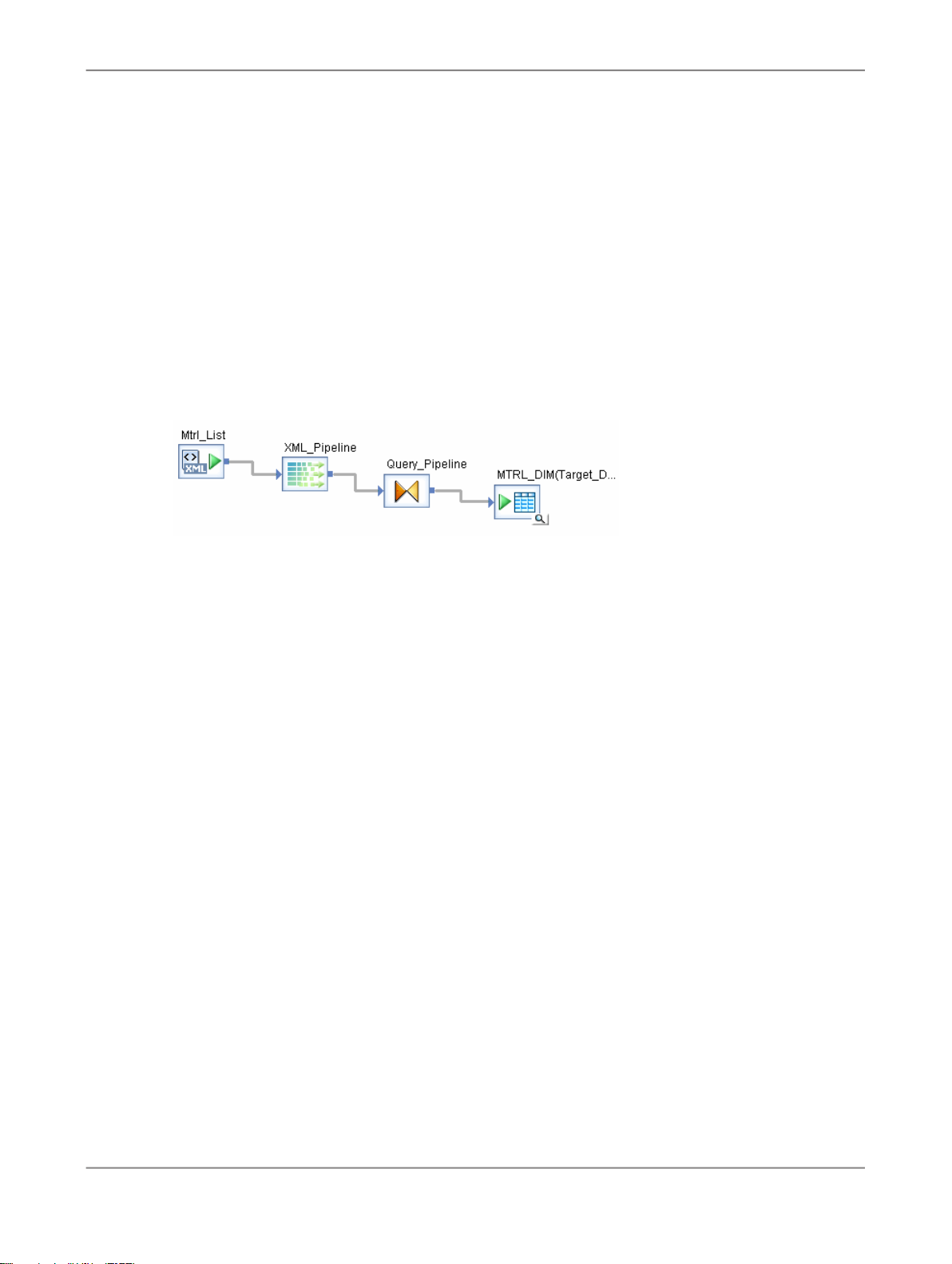
Populating the Material Dimension from an XML File
9.
Select Enable Validation to enable comparison of the incoming data to the stored DTD format.
10.
Click the back arrow to return to the data flow.
11.
In the object library on the Transforms tab, expand the Data Integrator transforms.
12.
Drag the XML_Pipeline transform into the DF_Mtrl_Pipe definition workspace, drop it to the right of
Mtrl_List source.
13.
In the object library on the Transforms tab, expand the Platform transforms.
14.
Drag the Query transform into the workspace, drop it to the right of XML_Pipeline, and name the
query Query_Pipeline.
15.
From the list of tables in the object library for the Target_DS datastore, drag the MTRL_DIM table
to the workspace, drop it to the right of Query_Pipeline, and click Make Target.
16.
Connect the icons to indicate the flow of data from the source XML file through the XML_Pipeline
and Query_Pipeline transforms to the target table.
7.6.2 To define the details of XML_Pipeline and Query_Pipeline
1.
Click XML_Pipeline to open the transform editor. Notice the nested structure of the source in the
Schema In pane.
2.
Drag the MTRL_ID, MTRL_TYPE, IND_SECTOR, MRTL_GROUP, and SHORT_TEXT columns to
the output schema.
Note:
Unlike the Query transform, the XML_Pipeline transform allows you to map a nested column directly
to a flat target.
2010-12-0277
Page 78

Populating the Material Dimension from an XML File
3.
Return to the data flow (either click the back arrow or click DF_Mtrl_Pipe in the project area).
4.
Click Query_Pipeline to open the query editor.
5.
Drag each "Schema In" column to the corresponding columns in the output schema. If you are
remapping the fields, choose Remap Column from the menu that appears. The Remap Column
option preserves the name and data type in Schema Out.
Schema Out column nameSchema In column name
MTRL_IDMTRL_ID
MTRL_TYPMTRL_TYPE
IND_SECTORIND_SECTOR
MTRL_GRPMTRL_GROUP
DESCRSHORT_TEXT
6.
In the project area, click the MTRL_DIM table to open the target editor. In the Options tab, select
the Delete data from table before loading option.
7.
In the project area, click DF_MTRL_Pipe to return to the data flow.
8.
From the Validation menu, click Validate > All Objects in View.
2010-12-0278
Page 79

Populating the Material Dimension from an XML File
You should see warning messages indicating that data types will be converted (which is acceptable
because you chose to preserve the data types from the output schema). Review the warning
messages and continue.
9.
In the project area, right-click JOB_Mtrl_Pipe and click Execute.
10.
If prompted to save your work, click OK.
11.
In the "Execution Properties" dialog box, click OK.
12.
After the job completes, ensure there are no error or warning messages.
13.
To view the captured sample data, in the project area select the data flow to open it in the workspace.
Click the magnifying glass on the target MTRL.DIM table to view its six rows.
Or, use a query tool to check the contents of the MTRL.DIM table.
7.7 Summary and what to do next
You have now populated four tables in the sample data warehouse:
• Sales organization dimension from a flat file
• Time dimension using the Date Generation transform
• Customer dimension from a relational table
• Material dimension from a nested XML file
In the next section you will populate the sales fact table.
Related Topics
• Designer Guide: Nested Data
• Reference Guide: Transforms
2010-12-0279
Page 80

Populating the Material Dimension from an XML File
2010-12-0280
Page 81
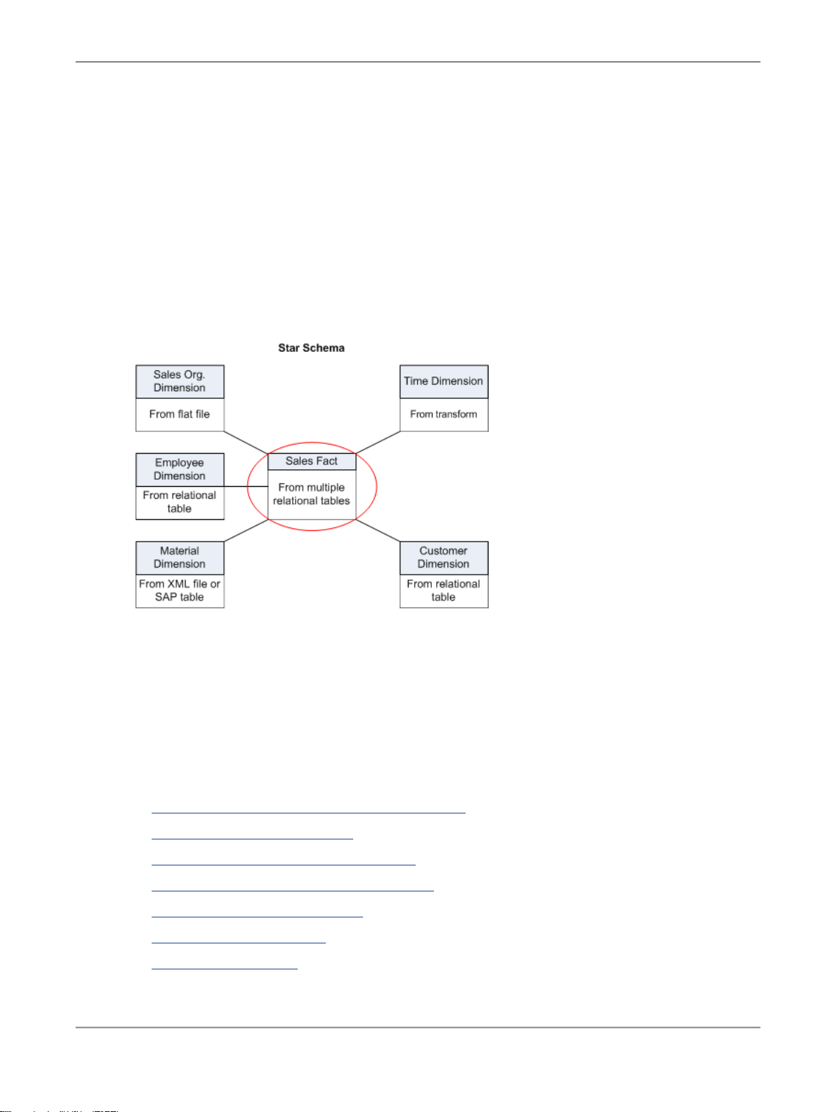
Populating the Sales Fact Table from Multiple Relational Tables
Populating the Sales Fact Table from Multiple Relational
Tables
In this section, you will populate the sales fact table in your sales data warehouse.
The exercise joins data from two source tables and loads it into an output table. Data Services features
introduced in this exercise are:
• Using the query transform FROM clause to perform joins
• Adding columns to an output table
• Mapping column values using Data Services functions
• Using metadata reports to view the sources for target tables and columns
The tasks in this section include:
• Adding the SalesFact job, work flow, and data flow
• Defining the SalesFact data flow
• Defining the details of the Query transform
• Defining the details of the lookup_ext function
• Validating the SalesFact data flow
• Executing the SalesFact job
• Using metadata reports
2010-12-0281
Page 82

Populating the Sales Fact Table from Multiple Relational Tables
• Enabling metadata reporting
• Viewing Impact and Lineage Analysis
8.1 Exercise overview
In this exercise, you will:
• Populate the SalesFact table from two source tables:
• Table SalesItem - columns Cust_ID and Order_Date
• SalesOrder - columns Sales_Order_Number, Sales_Line_Item_ID, Mtrl_ID, and Price.
• Use the FROM clause in the Query transform to join the two source tables and add a filter to bring
a subset of sales orders to the target.
• Use the LOOKUP_EXT() function to obtain the value for the Ord_status column from the Delivery
source table rather than from the SalesOrder table.
• Use metadata reports to view:
• Names of the source tables that populate the target SalesFact table
• Names of source columns that populate the target columns
8.2 Adding the SalesFact job, work flow, and data flow
8.2.1 To add the SalesFact job objects
1.
Add a new job and name it JOB_SalesFact. (For details, see Adding a job.)
2.
Add a work flow and name it WF_SalesFact. (For details, see Adding a work flow.)
3.
Click the WF_SalesFact name to open it in the workspace.
4.
Add a data flow to the work flow definition and name it DF_SalesFact.
8.3 Defining the SalesFact data flow
2010-12-0282
Page 83

Populating the Sales Fact Table from Multiple Relational Tables
Now you will define the data flow to populate the sales fact table in the data warehouse.
8.3.1 To define the data flow that will generate the sales fact table
1.
Click the name of the DF_SalesFact data flow to open the data flow definition.
2.
In the object library, click the Datastores tab. From the ODS_DS datastore, drag and drop the
SalesItem table to the left side of the workspace and click Make Source.
3.
Drag and drop the SalesOrder table to the left side of the workspace and click Make Source.
4.
Click the query transform icon in the tool palette.
5.
Click to the right of the tables in the workspace to place the query transform.
6.
From the list of tables in the Target_DS datastore, drag and drop the SALES_FACT table into the
workspace to the right of the query and click Make Target.
7.
From the Tools menu, click Options. Expand the Designer category and click Graphics. Here you
can change the appearance of your display. In the Workspace Flow Type menu, click Data Flow.
Click the line type Horizontal/Vertical. Click OK.
8.
In the data flow workspace, connect the icons to indicate the flow of data as shown in the following
diagram.
8.4 Defining the details of the Query transform
8.4.1 To define the details of the query, including the join between source tables
2010-12-0283
Page 84

Populating the Sales Fact Table from Multiple Relational Tables
1.
Open the query editor.
2.
In the FROM tab, in the Join pairs area, select ODS_SALESORDER from the Left drop-down list.
3.
Select ODS_SALESITEM from the Right drop-down list.
The relationship between the SalesItem and SalesOrder sales tables is defined by the common
column Sales_Order_Number. The Join option generates a join expression based on primary/foreign
keys and column names.
The resulting relationship appears in the From clause text box:
SALESITEM.SALES_ORDER_NUMBER = SALESORDER.SALES_ORDER_NUMBER
4.
Click the smart editor icon.
5.
In the Smart Editor, type the following text. Use all uppercase, as shown. This statement filters the
sales orders by date and brings one year's sales orders into the target. Also note that as you type
the function names, a pop-up window prompts you with options. To select an option that is highlighted,
press Enter (or double-click any option in the list).
AND ODS_SALESORDER.ORDER_DATE >= to_date('2007.01.01','yyyy.mm.dd')
AND ODS_SALESORDER.ORDER_DATE <= to_date('2007.12.31','yyyy.mm.dd')
6.
7.
DER
SALESITEM
Click OK.
Map the following source columns to output columns. Remember that to map the contents of a
column, select the column in the source schema and drag it to the target schema.
Target Column (in
order)DescriptionData typeColumnSource Table
CUST_IDCustomer IDvarchar(10)CUST_IDSALESOR-
ORDER_DATE
SLS_DOC_DATEOrder datedate or datetime (Sybase
ASE)
SLS_DOC_NOSales order
SLS_DOC_LINE_NOLine item
DER_NUMBER
LINE_ITEM_ID
varchar(10)SALES_OR-
number
varchar(6)SALES_
number
MATERIAL_NOMaterial IDvarchar(18)MTRL_ID
varchar(10)PRICE
NET_VALUEOrder item
price
8.5 Defining the details of the lookup_ext function
2010-12-0284
Page 85

Populating the Sales Fact Table from Multiple Relational Tables
You will take the Sales_Fact table order status value (column ORD_STATUS) from the Delivery source
table (column DEL_ORDER_STATUS) rather than from the SalesOrder table.
8.5.1 To use a lookup_ext function for order status
1.
In the query editor, select the ORD_STATUS column in the target schema.
2.
On the Mapping tab, click the Functions button.
3.
In the Select Function window, in the Function categories box, click Lookup Functions.
4.
Click lookup_ext from Function name.
5.
Click Next.
6.
To define the LOOKUP_EXT() function, complete the dialog box with the values shown in the following
graphic. To add an expression, you can either drag column names into the Expression and Default
fields or click the ellipses button to open the Smart Editor.
a. In the Lookup table drop-down list, select ODS_DS. Select the Delivery source table and click
OK. The lookup table is where the LOOKUP_EXT() function will obtain the value to put into the
ORD_STATUS column.
b. In the "Available parameters" area, expand the "Lookup table" and "Input schema" to display the
columns in the Delivery table and SalesItems table, respectively.
7.
Set up the first Condition. The conditions identify the row to look up in the lookup table. You need
two conditions in this exercise because each item in an order can have a different order status.
a. Drag the DEL_SALES_ORDER_NUMBER column from the Delivery table to the Column in
lookup table under "Condition".
b. Verify the operator is equal to (=).
c. Click the ellipses next to the Expression field to open the Smart Editor. On the Data tab, expand
the SalesItem table. Drag the SALES_ORDER_NUMBER column to the right side and click OK.
8.
Similarly, set the second condition for DEL_ORDER_ITEM_NUMBER equal to
ODS_SALESITEM.SALES_LINE_ITEM_ID. You can either drag the SALES_LINE_ITEM_ID column
into the Expression field, or you can click the ellipses button to open the Smart Editor to add the
column to the expression.
9.
The "Output" parameter specifies the column in the lookup table that contains the value to put in the
ORD_STATUS column in the query. For the "Output", drag the DEL_ORDER_STATUS column from
the ODS_Delivery under "Column in Lookup table".
2010-12-0285
Page 86

Populating the Sales Fact Table from Multiple Relational Tables
10.
Click Finish.
The final lookup function should read as follows (word wrapping is optional):
lookup_ext(
[ODS_ds.DBO.DELIVERY, 'PRE_LOAD_CACHE', 'MAX'],
[ DEL_ORDER_STATUS ],
[ 'N/A' ],
[ DEL_SALES_ORDER_NUMBER,'=',
ODS_SALESITEM.SALES_ORDER_NUMBER,
DEL_ORDER_ITEM_NUMBER, '=', ODS_SALESITEM.SALES_LINE_ITEM_ID ])
11.
Click the Back arrow in the tool bar.
8.6 Validating the SalesFact data flow
Next verify that the data flow has been constructed properly.
Click the Validate All button on the toolbar.
If your design contains syntax errors, a dialog box appears with a message describing the error.
As before, warning messages are OK.
2010-12-0286
Page 87

Populating the Sales Fact Table from Multiple Relational Tables
8.7 Executing the SalesFact job
As you did in previous exercises, execute the job named JOB_SalesFact. No error messages should
appear in the status window. You might see a warning message indicating that a conversion from a
date to datetime value occurred.
In the project area, click DF_SalesFact to view it in the workspace. Click the magnifying-glass icon on
the target SALES_FACT table to view its 17 rows.
8.8 Using metadata reports
Using the metadata reporting tool, you can easily browse reports about metadata associated with a
Data Services job. The metadata reporting tool is a Web-based application.
8.8.1 Enabling metadata reporting
Before you can use the tool, you must configure a repository connection in the Administrator to make
the repository available for metadata reporting.
8.8.1.1 To add a repository connection in the Administrator
1.
From the Start menu, click Programs > SAP BusinessObjects Data Services XI 4.0 > Data
Services Management Console.
2.
Log in with the user name admin and the password admin.
3.
Choose Administrator.
4.
Expand the Management tree.
5.
Click Repositories.
6.
Click Add.
7.
Enter the appropriate information for the repository.
• Repository Name — Logical name for a repository (used in the Web Administrator only)
• Database type — The type of database storing your repository
2010-12-0287
Page 88

Populating the Sales Fact Table from Multiple Relational Tables
• Machine Name — Host name on which the database server is running
• Database Port — Port number of the database or data source
• Service Name/SID, Database name, Server name, or Data source — Depends on the database
type you select (refer to the names you used in Tutorial setup).
• User name — The user or owner name for the database or data source (refer to Tutorial setup)
• Password — The user's account password for the database or data source (refer to Tutorial
setup)
8.
Click Test to verify the connection with the database information you have specified for the repository.
9.
Click Apply. The Administrator validates the repository connection information and displays it on
the List of Repositories page.
8.8.2 Viewing Impact and Lineage Analysis
In this example, you will use the metadata reporting tool to view reports about the SALES_FACT table
to identify when the table was last updated and what are the source tables and column mappings.
8.8.2.1 To open the Impact and Lineage Analysis tool
1.
Open the Designer.
2010-12-0288
Page 89

Populating the Sales Fact Table from Multiple Relational Tables
2.
From the Tools menu, click Data Services Management Console.
A browser window opens that shows the Management Console home page.
Note:
If you get a login screen, enter the user name admin and the password admin.
You can also open the Management Console from the Start menu by clicking Start > Programs >
SAP BusinessObjects Data Services XI 4.0 > Data Services Management Console.
8.8.2.2 To determine the sources for the SALES_FACT target table
1.
Click Impact & Lineage Analysis.
2.
To ensure that Metadata Reports includes the most up-to-date information about sources for columns
in target tables, click Settings in the upper right corner.
a. Ensure that Repository contains your current repository name.
b. Click the Refresh Usage Data tab.
c. Ensure that Job Server contains your current Job Server name. Click the Calculate Column
Mapping button to determine where the data comes from for each column in the target tables.
You should receive the following successful message:
Column mappings are calculated successfully.
d. Click Close.
3.
Expand the Target_DS datastore.
A list of tables in the datastore displays.
4.
Expand "Data Flow Column Mapping Calculation" to view the calculation status of each data flow.
5.
Click the SALES_FACT table.
The Overview tab for Table: SALES_FACT opens on the right side of the browser window. This tab
displays general information about the table such as the date and time this target table was last
updated (Last Update Date).
6.
Click the Lineage tab.
The following Lineage tab displays the sources for the SALES_FACT target table. When you move
the pointer over a source table icon, the name of the datastore, data flow, and owner appear.
2010-12-0289
Page 90

Populating the Sales Fact Table from Multiple Relational Tables
7.
Expand the SALES_FACT table on the left side of the browser window to display a list of columns.
8.
Click the ORD_STATUS column to display information about it on the right side.
The following Lineage tab shows that the SALES_FACT.ORD_STATUS column is based on
information in the source columns ODS_SALESITEM.SALES_LINE_ITEM_ID and
ODS_SALESITEM.SALES_ORDER_NUMBER.
These are the source columns that you defined in the condition for the LOOKUP_EXT() function in
Defining the details of the lookup_ext function.
You can print these reports by clicking the printer icon on the toolbar.
2010-12-0290
Page 91

Populating the Sales Fact Table from Multiple Relational Tables
8.9 Summary and what to do next
You have now populated five tables in the sales data warehouse:
• Sales org dimension from a flat file
• Time dimension using the Date Generation transform
• Customer dimension from a relational table
• Material dimension from a nested XML file
• Sales fact table from two relational tables
The next section introduces you to Data Services' capability to capture changed data.
For more information about metadata reports, see the
For more information about the other topics covered in this section, see the
Related Topics
• Reference Guide: Transforms, Query
• Reference Guide: Functions and Procedures, lookup_ext
Management Console Guide
Designer Guide
.
.
2010-12-0291
Page 92

Populating the Sales Fact Table from Multiple Relational Tables
2010-12-0292
Page 93

Changed-Data Capture
Changed-Data Capture
This section introduces the concept of changed-data capture (CDC). You use CDC techniques to identify
changes in a source table at a given point in time (such as since the previous data extraction). CDC
captures changes such as inserting a row, updating a row, or deleting a row. CDC can involve variables,
parameters, custom (user-defined) functions, and scripts.
9.1 Exercise overview
You will create two jobs in this exercise. The first job (Initial) initially loads all of the rows from a source
table. You will then introduce a change to the source table. The second job (Delta) identifies only the
rows that have been added or changed and loads them into the target table. You will create the target
table from a template.
Both jobs contain the following objects.
• An initialization script that sets values for two global variables: $GV_STARTTIME and $GV_ENDTIME
• A data flow that loads only the rows with dates that fall between $GV_STARTTIME and
$GV_ENDTIME
• A termination script that updates a database table that stores the last $GV_ENDTIME
The source table in this exercise, Customer, contains a column called Cust_timestamp that a user would
modify when creating or updating a row. The job checks this datetime, determines if it is later than the
last time the job ran, and if so, passes only that row to the target template table.
The target database contains a job status table called CDC_time that stores the last value of
$GV_ENDTIME. When you execute the delta-load job, it updates that value to use for the next execution.
Therefore, this section introduces the following new concepts:
• Changed-data capture
• Global variables
• Scripts
• Template tables
2010-12-0293
Page 94

Changed-Data Capture
9.2 Adding and defining the initial-load job
First create the job that initially loads the target table.
JOB_CDC_Initial will contain an initialization script, a data flow, and a termination script.
This section includes the following tasks:
• Adding the job and defining global variables
• Adding and defining the work flow
• Defining the data flow
9.2.1 Adding the job and defining global variables
Variables are symbolic placeholders for values. You can increase the flexibility and reusability of work
flows and data flows using variables when you design your jobs.
In this exercise, you will create two global variables that serve as placeholders for time stamps (a start
time and an end time). These time stamps will identify which rows in a source have been updated and
therefore will be captured as being changed.
Global variables are exclusive within the context of the job in which they are created. Add and define
the job and job-level global variables as follows.
9.2.1.1 To add the job and define the global variables
1.
To the Class_Exercises project, add a job named JOB_CDC_Initial.
2.
Verify the job is open by clicking its name in the project area.
3.
Click Tools > Variables.
The "Variables and Parameters" window appears. Notice that the job name displays in the Context
box.
4.
Right-click Global Variables and click Insert.
Data Services adds a variable with an automatically generated name. A focus box appears around
the name cell and the cursor shape changes to an arrow with a yellow pencil.
5.
Click the name cell to edit the name of the new global variable. Name the variable $GV_STARTTIME.
2010-12-0294
Page 95

Changed-Data Capture
6.
Click the data type cell and select datetime.
7.
Repeat this procedure to create the global datetime variable $GV_ENDTIME.
8.
Close the "Variables and Parameters" window.
9.2.2 Adding and defining the work flow
9.2.2.1 To add and define the work flow
1.
With the JOB_CDC_Initial definition open in the workspace, add a work flow named
WF_CDC_Initial.
2.
Open the work flow definition for WF_CDC_Initial by clicking its name in the project area.
3.
Click the script icon on the tool palette and place a script on the left side of the workspace. Name it
SET_START_END_TIME.
4.
Add a data flow to the right of the script and name it DF_CDC_Initial.
5.
Add another script to the right of DF_CDC_Initial and name it UPDATE_CDC_TIME_TABLE.
6.
Connect the two scripts to DF_CDC_Initial.
9.2.2.2 Defining the set and update time scripts
When typing scripts, be sure to follow the date syntax required by your database.
9.2.2.2.1 To define the workflow scripts
1.
In the object library, open the Customer source table by double-clicking it. Click the View Data tab.
To view the entire table, click the Open in new window icon.
Notice the oldest timestamp in the Cust_timestamp column is 2008.03.27 00:00:00.
2.
In the project area, click WF_CDC_Inital to go back to its definition in the workspace.
3.
Click the SET_START_END_TIME script's name to open the script editor. This script defines the
initial start and end times. To capture all rows in the source, set the start time global variable as
datetime 2008.01.01 00:00:000. Set the end time global variable as datetime sysdate (the current
datetime).
2010-12-0295
Page 96

Changed-Data Capture
For example:
$GV_STARTTIME = '2008.01.01 00:00:000';
$GV_ENDTIME = sysdate();
4.
Click the Validate icon to validate the script.
5.
Close the script editor for SET_START_END_TIME.
6.
Click the UPDATE_CDC_TIME_TABLE script name to open the script editor. This script resets the
$GV_ENDTIME value in the CDC_time table.
For example for MS SQL Server, type the following:
sql('Target_DS', 'DELETE FROM TARGET.CDC_TIME');
sql('Target_DS', 'INSERT INTO TARGET.CDC_TIME VALUES ({$GV_ENDTIME})');
Note:
Ensure that the user name in your script matches the user name defined for the table.
For example for Oracle, type the following:
sql('Target_DS', 'DELETE FROM TARGET.CDC_TIME');
sql('Target_DS', 'INSERT INTO TARGET.CDC_TIME VALUES (to_date({$GV_ENDTIME},\'YYYY.MM.DD HH24:MI:SS\'))');
7.
Click the Validate icon to validate the script. The warning message that data types will be converted
is acceptable (Data Services preserves the data type in the output schema).
9.2.2.3 Defining the data flow
Next define the data flow. The target table for this data flow will be a template table. When you use a
template table, you do not have to specify the table's schema or import metadata. Instead, during job
execution, Data Services has the DBMS create the table with the schema defined by the data flow.
Template tables appear in the object library under each datastore. To add a template table to a target
datastore, drag the template table icon from that datastore to the workspace and name it.
9.2.2.3.1 To define the data flow
1.
In the project area, click the name of data flow DF_CDC_Initial.
2.
In the object library from the ODS_DS datastore, drag the Customer table to the workspace and
click Make Source.
3.
Add a query to right of the source table and name it QryCDC.
4.
From the Target_DS datastore, drag the Template Tables icon to the right of the query in the
workspace.
5.
In the "Create template" dialog box, name the template table CUST_CDC.
6.
Connect the source, query, and target together.
7.
Click the name of the target table CUST_CDC to open its definition.
8.
Click the Options tab.
9.
Select the check box Delete data from table before loading.
2010-12-0296
Page 97

Changed-Data Capture
10.
Click the Back arrow on the tool bar to close the target table definition and return to the data flow
view.
9.2.2.3.2 To define the data flow query
1.
In the project area, click QryCDC to open the query editor.
2.
Drag the following columns from the Schema In pane to the Schema Out pane:
CUST_ID
CUST_CLASSF
NAME1
ZIP
CUST_TIMESTAMP
3.
On the Where tab, type:
(ODS_CUSTOMER.CUST_TIMESTAMP >= $GV_STARTTIME) and
(ODS_CUSTOMER.CUST_TIMESTAMP <= $GV_ENDTIME)
Note:
You can drag the column CUSTOMER.CUST_TIMESTAMP from Schema In to the Where tab.
When you type $, a list appears where you can select the $GV_STARTTIME and $GV_ENDTIME
variable names.
4.
Click the Validate icon on the toolbar to validate the query.
5.
Correct any errors and close the "Output" window.
6.
In the project area, click JOB_CDC_Initial.
7.
Click the Validate All icon on the toolbar and correct any errors. As before, warning messages are
ok.
8.
Click the Save All toolbar icon to save the job.
9.
Close the job, work flow, data flow, template table target editor, and query editor windows.
9.3 Adding and defining the delta-load job
To build the delta-load job more quickly, you will first replicate the initial-load data flow and modify it.
9.3.1 To add the delta-load data flow
1.
In the object library, click the Data Flows tab.
2.
Right-click DF_CDC_Initial and click Replicate.
2010-12-0297
Page 98

Changed-Data Capture
3.
Right-click the copy, click Rename, and name the data flow DF_CDC_Delta.
4.
Double-click the name of the data flow in the object library to open it in the workspace.
5.
Click the name of the target table CUST_CDC.
6.
Click the Options tab.
7.
Clear the check boxes for the Delete data from table before loading and Drop and re-create
table options.
9.3.2 To add the job and define the global variables
1.
In the project area, right-click the Class_Exercises project and click New Batch Job.
2.
Name the job JOB_CDC_Delta.
3.
Open JOB_CDC_Delta by clicking its name in the project area.
4.
Click Tools > Variables.
The "Variables and Parameters" window appears. Notice that the job name displays in the Context
box.
5.
Right-click Global Variables and click Insert.
Data Services adds a variable with an automatically generated name. A focus box appears around
the name cell and the cursor shape changes to an arrow with a yellow pencil.
6.
Click the name cell to edit the name of the new global variable. Name the variable $GV_STARTTIME.
7.
Click the data type cell and select datetime.
8.
Repeat this procedure to create the global datetime variable $GV_ENDTIME.
9.
Close the "Variables and Parameters" window.
9.3.3 To add and define the work flow
1.
Add a work flow to JOB_CDC_Delta and name it WF_CDC_Delta.
2.
Click the name of the work flow in the project area to open it.
3.
Click the script icon in the tool palette and add it to the work flow. Name the script
SET_NEW_START_END_TIME.
4.
From the object library Data Flows tab, drag DF_CDC_Delta to the work flow.
5.
Add another script to the right of DF_CDC_Delta and name it UPDATE_CDC_TIME_TABLE.
6.
Connect the scripts and data flow together.
2010-12-0298
Page 99

Changed-Data Capture
9.3.4 To define the scripts
1.
Click the name of the SET_NEW_START_END_TIME script to open the script editor.
2.
For the delta-load job, you define the start-time global variable to be the last time stamp recorded
in the CDC_time table.
For example for MS SQL Server:
$GV_STARTTIME = to_date(sql('Target_DS', 'SELECT LAST_TIME FROM TARGET.CDC_TIME'), 'YYYY-MM-DD HH24:MI:SS');
$GV_ENDTIME = sysdate();
For example for Oracle:
$GV_STARTTIME = sql('Target_DS','SELECT to_char(LAST_TIME,\'YYYY.MM.DD HH24:MI:SS\') FROM TARGET.CDC_TIME');
$GV_ENDTIME = sysdate();
3.
Click the UPDATE_CDC_TIME_TABLE script's name to open the script editor. This script resets the
$GV_ENDTIME value in the CDC_time table.
For example for MS SQL Server:
sql('Target_DS', 'UPDATE TARGET.CDC_TIME SET LAST_TIME ={$GV_ENDTIME}');
For example for Oracle:
sql('Target_DS', 'INSERT INTO TARGET.CDC_TIME VALUES (to_date({$GV_ENDTIME},\'YYYY.MM.DD HH24:MI:SS\'))');
4.
Click the job name and click the Validate All icon. Correct any errors (warnings are ok).
5.
Click the Save All toolbar icon and click OK to save the job.
9.4 Executing the jobs
First you will execute the initial-load job and view the results to verify that the job returned all rows from
the source. Then you will open the source table and introduce a change. Finally, you will run the
delta-load job to extract only the changes and update the target.
9.4.1 To execute the initial-load job
1.
Use a table-editing tool (e.g. MS SQL Server Management Console) to view the data in the Customer
source table. There are 12 rows.
2.
In Data Services, right click JOB_CDC_Initial and click Execute.
3.
In the "Execution Properties" window, click OK.
2010-12-0299
Page 100

Changed-Data Capture
4.
After successful execution, click the monitor button and view the Row Count column to determine
how many rows were loaded into the target table. The job should return all 12 rows.
You can also check this row count by opening the data flow and clicking the View Data icon on the
target table.
9.4.2 To change the source data
1.
Use a table-editing tool (e.g. Oracle DBA Studio or MS SQL Server Enterprise Manager) to view
the data in the Customer source table.
2.
Add a row to the table with the following data.
Note:
If your database does not allow nulls for some fields, copy the data from another row. You will fix
the ZIP value in the next section.
ValueColumn name
ZZ01Cust_ID
ZZCust_Classf
EZ BIName1
ZZZZZZIP
Cust_Timestamp
3.
Save the table.
The current date and time in the appropriate format for your
database, for example 5/5/2009 12:25:00
9.4.3 To execute the delta-load job
1.
In Data Services, execute JOB_CDC_Delta.
2.
View the results by opening the monitor log. The row count should be 1.
3.
Open the data flow editor and view the data in the target table. The new row should appear in the
target data after the 12 rows that JOB_CDC_Initial loaded.
2010-12-02100
 Loading...