

Page 1
1
S3602 Series Vector Network Analyzer
User Manual
Saluki Technology Inc.
Page 2
Tel: 886.2.2175 2930 Email: [email protected]
www.salukitec.com
2
Preface
Thanks for choosing S3602 Vector Network Analyzer produced by Saluki Technology Inc. Please read this user manual carefully for your
convenience.
We devote ourselves to meeting your demands, providing you high-quality measuring instrument and the best after-sales service. We
persist with “superior quality and considerate service”, and are committed to offering satisfactory products and service for our clients.
Manual No.
S36020301
Version
Rev01 2016.06
Saluki Technology
Manual Authorization
The information contained in this User Manual is subject to change without notice. The power to interpret the contents of and terms used
in this Manual rests with Saluki.
Saluki Tech owns the copyright of this User Manual which should not be modified or tampered by any organization or individual, or
reproduced or transmitted for the purpose of making profit without its prior permission, otherwise Saluki will reserve the right to
investigate and affix legal liability of infringement.
Precautions
"Warning" indicates danger. It reminds the user to pay attention to a certain operation process, operation method or similar situations.
Noncompliance with the rules or improper operation may result in personal injuries. You must fully understand the warning and all the
conditions in it shall be met before the next step
"Attention" indicates important prompts and no danger. It reminds the user to pay attention to a certain operation process, operation
method or similar situations. Noncompliance with the rules or improper operation may result in damage to the instrument or loss of
important data. You must fully understand the caution and all the conditions in it shall be met before the next step.
Page 3

Tel: 886.2.2175 2930 Email: [email protected]
www.salukitec.com
3
Contacts
Service Tel:
886.2.2175 2930
Website:
www.salukitec.com
Email:
Address:
No. 367 Fuxing N Road, Taipei 105,Taiwan (R.O.C.)
Page 4

Tel: 886.2.2175 2930 Email: [email protected]
www.salukitec.com
4
Content
1. Manual Guide...............................................................................................................................................................................6
1.1. About the Manual
..............................................................................................................................................................
6
1.2. Related Documents........................................................................................................................................................... 7
2. Overview
.....................................................................................................................................................................................
9
2.1. Product Overview
..............................................................................................................................................................
9
2.2. Safety Guide................................................................................................................................................................... 12
3. Introduction to Use
......................................................................................................................................................................
18
3.1. Preparation before Use.................................................................................................................................................... 18
3.2. Front Panel & Rear Panel
.................................................................................................................................................
30
3.3. Graphic User Interface
.....................................................................................................................................................
41
3.4. Trace, Channel and Window of Analyzer........................................................................................................................... 42
3.5. Data Analysis
..................................................................................................................................................................
44
3.6. Data output..................................................................................................................................................................... 65
4. Measurement setups.................................................................................................................................................................. 72
4.1. Resetting of Analyzer
.......................................................................................................................................................
72
4.2. Selection of Measurement Parameter................................................................................................................................76
4.3. Setting of Frequency Range
.............................................................................................................................................
80
4.4. Setting of Signal Power Level........................................................................................................................................... 81
4.5. Setting of Sweep............................................................................................................................................................. 83
4.6. Trigger Mode...................................................................................................................................................................87
4.7. Setting of Data Format and Scale..................................................................................................................................... 93
4.8. Observation of Multiple Tracks and Opening of Multiple Channels
.......................................................................................
97
4.9. Setting of Analyzer Display
.............................................................................................................................................
100
5. Menu....................................................................................................................................................................................... 106
5.1. Menu structure
...............................................................................................................................................................
106
5.2. Description of menu....................................................................................................................................................... 113
6. Measurement Optimization
........................................................................................................................................................
166
6.1. Reduction of Accessory Influence....................................................................................................................................166
6.2. Improvement of Reflection Accuracy of Low-loss 2-port Device
.........................................................................................
167
6.3. Increase of Dynamic Range
............................................................................................................................................
169
6.4. Improvement of Measurement Results of Electrical Long Device....................................................................................... 171
6.5. Improvement of Phase Measurement Accuracy................................................................................................................172
6.6. Reduction of trace Noise................................................................................................................................................ 178
6.7. Increase of Data Point Number.......................................................................................................................................181
6.8. Improvement of Measurement Stability
............................................................................................................................
182
6.9. Increase of sweep Speed............................................................................................................................................... 184
Page 5

Tel: 886.2.2175 2930 Email: [email protected]
www.salukitec.com
5
6.10. Improvement of Efficiency of Multi-state Measurement....................................................................................................187
6.11. Rapid Data Transmission
..............................................................................................................................................
188
6.12. Use of Macro...............................................................................................................................................................189
7. Calibration................................................................................................................................................................................192
7.1. Calibration Overview
......................................................................................................................................................
192
7.2. Selection of Calibration Type...........................................................................................................................................193
7.3. Calibration Guide
...........................................................................................................................................................
195
7.4. High-accuracy Measurement Calibration
..........................................................................................................................
198
7.5. Measurement Errors...................................................................................................................................................... 199
7.6. Editing of Calibration Kit Definition
...................................................................................................................................
202
7.7. 7.7 Standard Calibration Kit............................................................................................................................................ 210
7.8. TRL Calibration
..............................................................................................................................................................
212
7.9. Fixture Compensation Calibration
...................................................................................................................................
213
7.10. Electronic Calibration................................................................................................................................................... 221
8. Basis of Network Measurement
.................................................................................................................................................
225
8.1. Reflection Measurement.................................................................................................................................................225
8.2. Phase Measurement......................................................................................................................................................227
8.3. Amplifier Parameter Specifications..................................................................................................................................229
8.4. Complex Impedance...................................................................................................................................................... 231
8.5. Group Delay
..................................................................................................................................................................
233
8.6. Absolute Output Power
...................................................................................................................................................
236
8.7. AM-PM Transformation...................................................................................................................................................237
8.8. Linear phase offset.........................................................................................................................................................240
8.9. Reverse Isolation........................................................................................................................................................... 241
8.10. Small Signal Gain and Flatness
.....................................................................................................................................
242
9. Remote control.........................................................................................................................................................................245
9.1. Basis of Remote Control
.................................................................................................................................................
245
9.2. Programmed Port and Configuration of Instrument
...........................................................................................................
259
9.3. Basic Programming Method of VISA Interface..................................................................................................................261
9.4. I/O Library..................................................................................................................................................................... 269
10. Fault Diagnoses and Repair.....................................................................................................................................................272
10.1. Operating principle
.......................................................................................................................................................
272
10.2. Fault Diagnosis and Troubleshooting
.............................................................................................................................
273
10.3. Error Information..........................................................................................................................................................275
11. Technical Indicators and Measurement Methods
.......................................................................................................................
291
11.1. Technical Indicators......................................................................................................................................................291
11.2. Measurement Methods.................................................................................................................................................298
Page 6

Tel: 886.2.2175 2930 Email: [email protected]
www.salukitec.com
6
1. Manual Guide
This chapter summarizes the functions, structure and main contents of the user manual of S3602 vector network analyzers, and the
related documents for the user.
About manual
Related documents
1.1.About the Manual
The manual describes the purposes, performance indicators, basic operating theory, operating method, operation precautions, etc. of
S3602 vector network analyzers produced by Saluki Technology, to help you rapidly get familiar with and understand key points of the
instrument operation and use. Please read this User Manual carefully and follow its guidance.
Due to the limit of time and knowledge of the writer, there may be some omissions or errors, and you are welcome to correct any such
errors. We are sorry for the flaws which may cause your inconvenience.
The user manual includes the following chapters.
Overview
The chapter provides an overview of the characteristics and operation precautions of S3602 vector network analyzers, mainly including a
product overview and a safe operation guide.
Introduction
This chapter describes the preparations before operation of S3602 vector network analyzers, routine maintenance of the system and
instrument, overview of the front panel and the rear panel, operation interface, analyzer menus, tracks, channels, windows, and analysis
and saving of measurement data.
Measurement setups
This chapter describes various settings of the network analyzer in operation, including resetting of the analyzer, selection of
measurement parameters, setting of the frequency range, setting of the signal power level, setting of sweep, selection of the trigger mode,
selection of the data format and scale, viewing of several tracks, opening of several channels, and setting of the analyzer display.
Menu
This chapter describes the menu structure and items according to functional categories to facilitate query and reference.
Measurement optimization
This chapter describes how to optimize the measurement accuracy by means of proper settings, including reduction of accessory
impacts, improvement of the reflection accuracy of the low-loss 2-port device, increase of the dynamic range, improvement of the
measurement results of the electrical length and the measurement accuracy of the phase, reduction of the trace noise and receiver
crosstalk, increase of data points, improvement of the measurement stability, sweep speed, multi-status measurement efficiency and
rapid data transmission, use of macros, etc.
Calibration
This chapter introduces the calibration type and method of S3602 vector network analyzers to improve the accuracy of measurement.
Network measurement basics
Page 7

Tel: 886.2.2175 2930 Email: [email protected]
www.salukitec.com
7
This chapter describes the basic concepts and related theories of senior network parameter measurement.
Remote control
This section outlines the remote control of the instrument, so that the user can rapidly get to know how to remotely control the instrument.
It is divided into four sections: the program control basics describe the concepts related to program control, software configuration,
program-controlled port, SCPI commands, etc.; instrument port configuration describes the connection and software configuration of the
program-controlled port of S3602 vector network analyzers; basic programming of VISA interface provides an example of basic
programming with text illustration and example codes, so that the user can rapidly get to know the programming method; and I/O function
library describes the basic concepts of the instrument drive and the basic installation and configuration requirements of the
IVI-COM/IVI-C drive.
Fault diagnosis and repair
This section describes the overall operating theory, fault diagnosis and troubleshooting, and errors and repair.
Technical indicators and test methods
This section describes the main technical indicators of S3602 analyzers and the recommended test instructions for the user.
1.2.
Related Documents
The documents related to S3602 series vector network analyzer include:
User Manual
Program control document
Quick Start Guide
User Manual
This manual introduces the functions and operation methods of the instrument in details, including configuration, measurement, program
control, maintenance, etc. It aims to guide the user to comprehensively understand the functional characteristics and common test
methods of the instrument. It mainly includes the following chapters:
Manual Navigation
Overview
Introduction
Measurement setups
Menu
Measurement optimization
Calibration
Network measurement basics
Remote control
Fault diagnosis and repair
Technical indicators and measurement method
Page 8

Tel: 886.2.2175 2930 Email: [email protected]
www.salukitec.com
8
Program control document
This manual introduces the remote programming basis, SCPI basis, SCPI commands, programming examples, I/O drive function library,
etc. It aims to guide the user to rapidly and comprehensively know the program control commands and methods of the instrument. It
mainly includes the following chapters:
Remote control
Program control commands
Programming examples
Error illustration
Appendix
Quick Start Guide
This manual introduces the basic operations of configuration, start-up and measurement of the instrument, aiming to help the user rapidly
know the characteristics of the instrument and understand basic settings and operations. It mainly includes the following chapters:
Preparation for use
Typical application
Help
Page 9

Tel: 886.2.2175 2930 Email: [email protected]
www.salukitec.com
9
2. Overview
This chapter describes the main performance characteristics, purposes and technical indicators of S3602analyzers. It also includes the
precautions for proper operation, electrical safety, etc.
Product overview
Safe operation guide
2.1.Product Overview
S3602 series vector network analyzer is a new generation of vector network analyzer, launched by Saluki Technology. In the hardware,
new design concept and technical architecture are adopted, thus significantly improving key technical performance indicators such as the
overall scanning speed and dynamic range. In the software, the embedded computer with high-performance microprocessor chip and
platform environment based on Windows7 operating system are applied, thus greatly improving the overall interconnection and usability.
S3602 series vector network analyzers have multiple calibration modes such as frequency response, single port, response isolation,
enhanced response, double ports and electrical calibration, and multiple display modes such as the logarithmic amplitude, linearity
amplitude, standing wave, phase, group delay and Smith chart. It is equipped with various standard interfaces, such as USB, LAN, GPIB
and VGA. In addition to all measurement functions of the traditional vector network analyzer, the instrument can be used to test
comprehensive parameters of multiple functions such as the mixer/converter, active intermodulation distortion and harmonic distortion,
gain compression and two-dimensional sweep and S-parameter of the pulse network, and accurately measure the amplitude frequency
characteristics, phase frequency characteristics and group delay characteristics of the microwave network.
The instrument can be widely applied in measurement of the transmission/reception (T/R) module, dielectric material properties,
microwave pulse characteristics and photoelectric properties. It is an indispensable tester in research and production of the phased array
radar, communication, RF microwave device and other systems.
Product Features:
12.1-inch high-resolution touch screen;
Multiple calibration modes such as the frequency response, single port, frequency isolation, double ports, TRL and electrical
calibration;
16 display windows capable of displaying 8 traces at the same time, and 64 independent measurement channels to rapidly
implement complex test solutions;
Record/run (one-button operation), greatly simplifying the Measurement setups steps and improving the working efficiency;
Multiple display formats such as the logarithmic amplitude, linearity amplitude, standing wave, phase, group delay, Smith chart and
polar coordinates;
USB, GPIB, LAN and VGA interface;
Two options: single-source stimulus type 2-port vector network analyzer and double-source stimulus
type four-port vector network analyzer;
Multiple functions such as the pulse measurement, time domain measurement, mixer measurement, active intermodulation
distortion measurement, gain compression and two-dimensional scanning measurement, millimeter wave spreading, antenna and
RCS measurement reception.
1.Simple and intuitive humane user interface, facilitating operation and improving the test efficiency.
Page 10
Tel: 886.2.2175 2930 Email: [email protected]
www.salukitec.com
10
The touch screen, panel keys and mouse can be used to effectively guide the user to properly operate the instrument. The operation can
be made quick and intuitive in the Windows system, thus greatly improving the test efficiency.
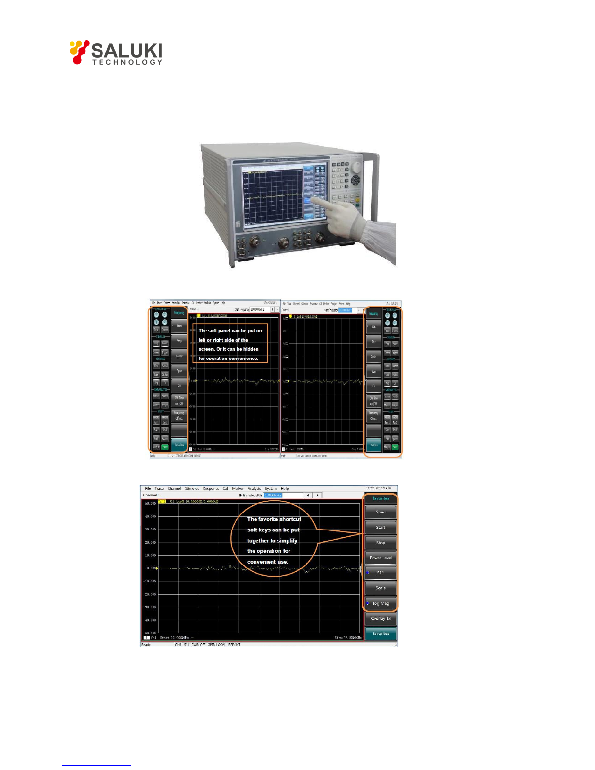
S3602 series vector network analyzers are equipped with a 12.1-inch 1280*800 touch screen, as shown in Fig. 2.1, to facilitate operation.
Fig. 2.1 12.1-inch 1280*800 Touch Screen
Fig. 2.2 Soft Panel Interface
Fig. 2.3 Soft Shortcut Keys
2.Multi-window multi-channel measurement display
S3602 series vector network analyzers support up to 64 channels, and as many as 16 measurement windows can be displayed at the
Page 11
Tel: 886.2.2175 2930 Email: [email protected]
www.salukitec.com
11
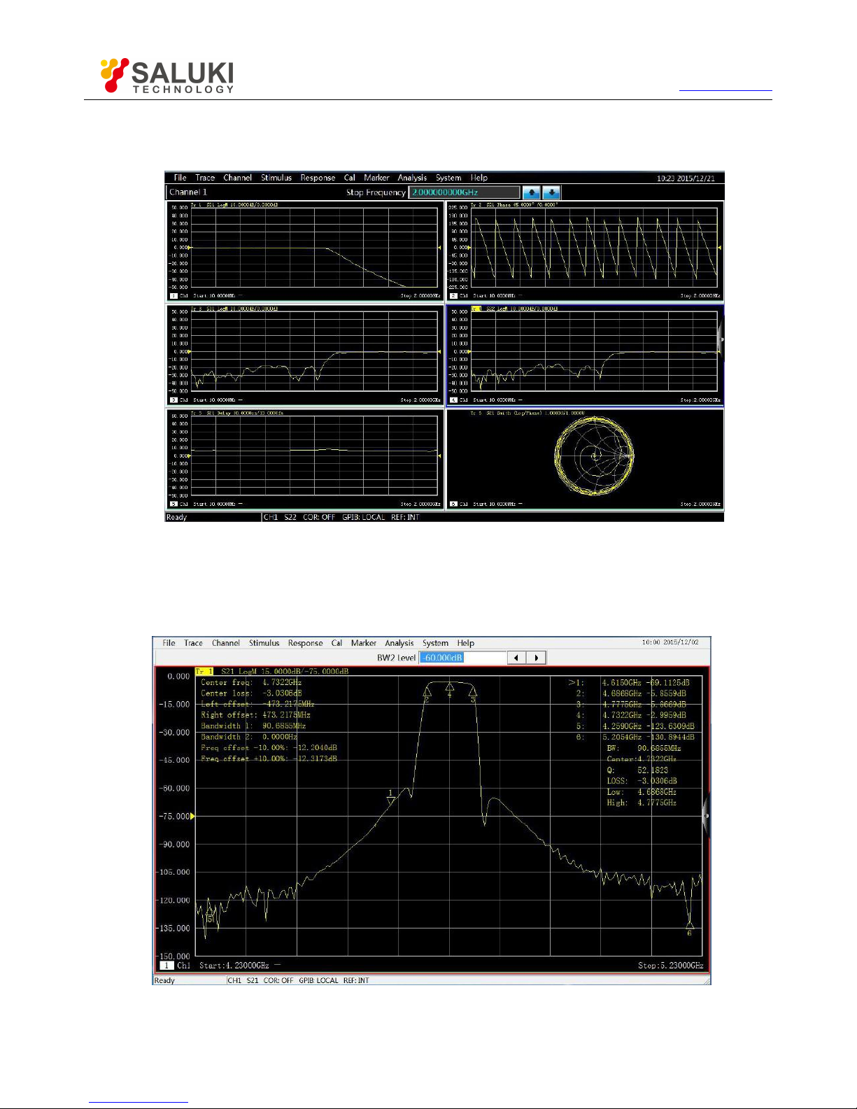
same time. Up to 8 test tracks can be displayed in each window, and frequent status calling is not required to measure several
parameters of the tested device, thus simplifying the test process.
Fig. 2.4 Multi-window Multi-channel Measurement Display
3.Wide dynamic range
S3602 series vector network analyzers are designed based on fundamental wave mixed reception, thus effectively expanding the
dynamic range of the overall test and meeting increasing test demands for the wide dynamic range.
Fig. 2.5 Filter Measurement Results
Page 12
Tel: 886.2.2175 2930 Email: [email protected]
www.salukitec.com
12
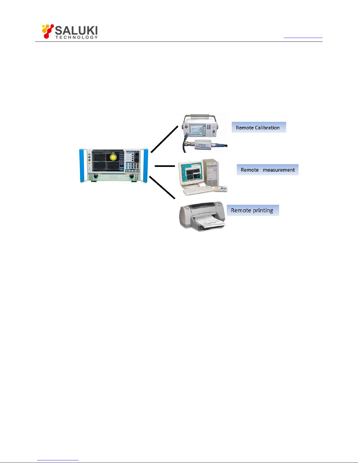
4.Automatic test
The automatic test can help to save a lot of time and effectively reduce the test cost in a flexible automation environment.
The vector network analyzer is controlled with SCPI commands to complete automatic tests.
Codes are directly executed from the vector network analyzer or external PC through a LAN or GPIB interface.
The application program can be directly run in the instrument, with no external PC.
Fig. 2.6 Automatic Test
1) GPIB interface
S3602 series vector network analyzers are equipped with a 24-pin D-type female GPIB connector, which conforms to the IEEE-488
standard and is used to send and receive GPIB/SCPI commands.
2) USB Interface
S3602 series vector network analyzers are equipped with nine high-speed USB interfaces (eight A-type interfaces and one B-type
interface) to facilitate the connection to the keyboard, mouse, printer, electronic calibrator and other peripherals with USB interfaces.
3) Printing function
S3602 series vector network analyzers have a powerful printing function, and are able to output or print the contents of the measurement
display into a specified file through a printer. A local or network printer with a LAN or USB interface can be used. Measurement results
can be printed after the printer is added to the Windows 7 operating system.
2.2.Safety Guide
Please carefully read and strictly follow the notes for attention below!
We will spare no effort to ensure that all production stages conform to the latest safety standards to guarantee the highest safety for
users. The design and test of our product and ancillary equipment thereof have been up to relevant standards of security; quality
assurance system has been established to monitor the product quality to ensure the consistency with such standards. Precautions
proposed in this User Manual should be followed to keep equipment intact and operations safe. Please do not hesitate to consult us if
you have any questions.
Page 13
Tel: 886.2.2175 2930 Email: [email protected]
www.salukitec.com
13
However, it is your responsibility to operate the product in a correct way. Please read and follow the safety instructions carefully before
operating the instrument. The instrument is applicable to the industrial and laboratory environment or field measurement. Pay attention to
the limitations for proper operation to avoid personal injury or property damage. We will not take any responsibility for any misuse or
inconsistency as required, and you are liable for any risks incurred by. Therefore follow the safety instructions to prevent from personal
injury or property damage. Please keep the basic safety instructions and product documentation safe and submit them to end users.
Safety signs
Operation status and location
Power safety
Operation precautions
Maintenance
Battery and power supply module
Transportation
Waste disposal/environment protection
2.2.1. Safety Signs
2.2.1.1. Product-related Signs
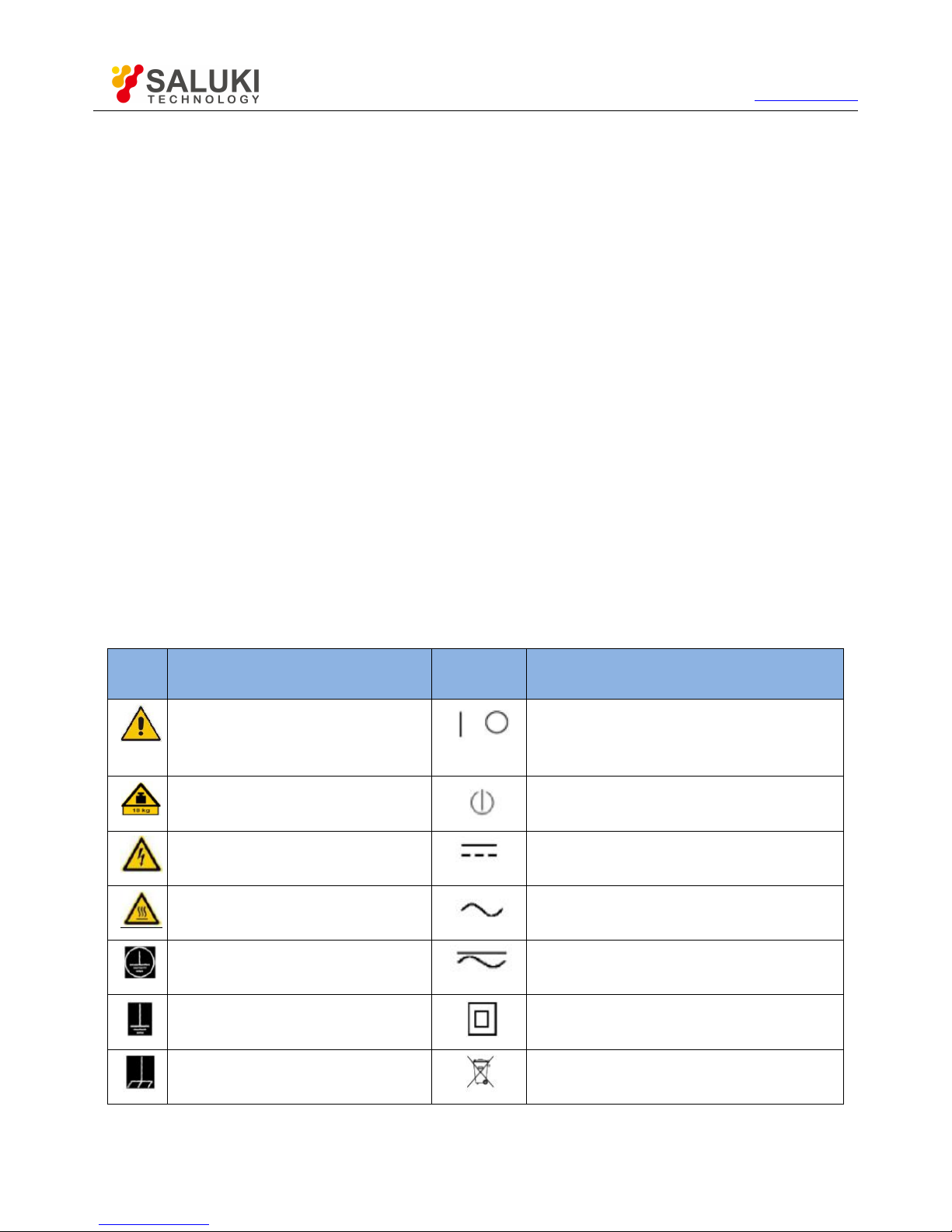
The safety signs of the instrument are as follows (Table 2.1).
Table 2.1 Instrument Safety Signs
Symbol
Meaning
Symbol
Meaning
Caution: the user should pay attention to the
information. The user should pay attention to the
operation information or instructions.
Power on/off
Caution: handle heavy equipment.
Standby indication
Danger! Be careful of electric shock!
Direct-current (DC) power
Warning! Be careful of surface heat.
Alternating-current (AC) power
Protect the conductive terminal.
Direct- current/alternating current power (DC/AC)
Grounding
Instrument reinforcement and insulation protection.
Earthing Terminal
EU mark of battery and accumulator.For details, refer to 1 of
"2.2.8 Waste disposal/environment protection".
Page 14
Tel: 886.2.2175 2930 Email: [email protected]
www.salukitec.com
14
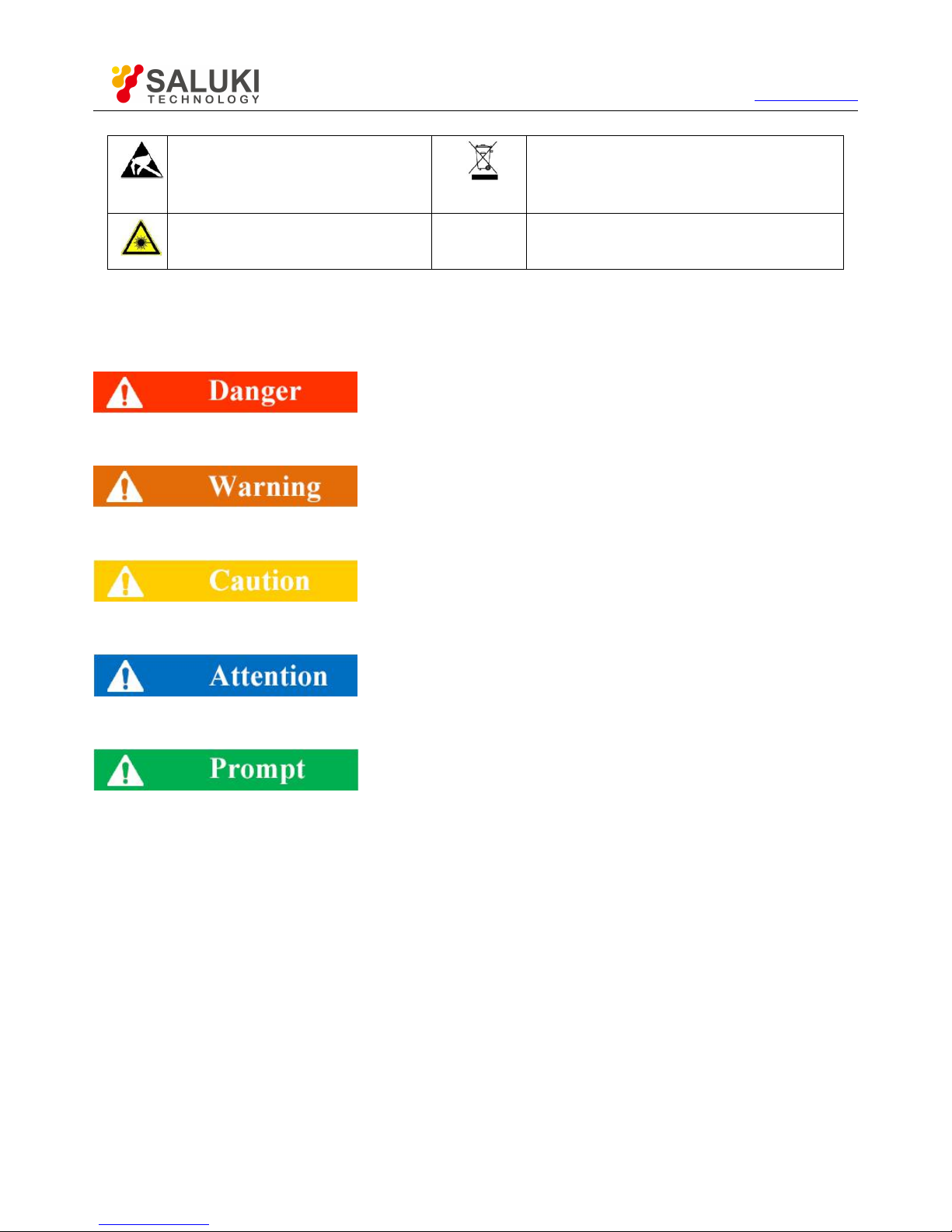
Caution: electrostatic sensitive device. Be careful.
EU mark for electronic parts to be collected separately For
details, refer to 2 of "2.2.8 Waste disposal/environment
protection".
Warning! Radiation. For details, refer to 7 of 2.2.4
"Operation Precautions" of this section.
2.2.1.2. Manual-related Signs
The following safety warning signs are used in the product manual to remind the user to operate the instrument safely and pay attention
to relevant information.
Danger sign: personal injury and equipment damage may be caused if no attention is paid.
Warning sign: personal injury and equipment damage may be caused if no attention is paid.
Caution sign: minor or moderate personal injury and equipment damage may be caused if no attention is paid.
Attention sign: it indicates important prompts but no danger.
Prompt sign: information of the instruction and operation.
2.2.2.
Operation Status and Location
Pay attention to the following items before operation:
1) Unless otherwise stated, S3602 series vector network analyzers should be placed steadily and operated indoor with protection of IP
2X. The maximum altitude must not exceed 2,000m in operation and 4,500m in transportation. The actual power supply voltage
may be the indicated voltage ± 10%, and the power supply frequency may be the indicated frequency ± 5%. Both the overvoltage
protection and the pollution intensity are Class 2.
2) Do not place the instrument on a wet surface, vehicle, cabinet, table and other objects which are not fixed and do not conform to the
load conditions. Place the instrument steadily and fix it on the solid object surface (such as the anti-static workbench).
3) Do not place the instrument on a heat dissipating surface (such as a radiator). The operating temperature must not exceed the
specified range of relevant indicators of the instrument. Overheating may result in electric shock, fire, etc.
Page 15

Tel: 886.2.2175 2930 Email: [email protected]
www.salukitec.com
15
2.2.3.
Power Safety
Precautions for the power supply of the instrument:
1) Ensure that the actual power supply voltage is the same as that marked on the instrument before powering-on. If the power supply
voltage is changed, replace the fuse of the instrument.
2) Refer to the power supply requirements on the rear panel of the instrument. Use three-core power cords. Ensure that the power
cord is grounded reliably. Floating or improper grounding may result in damage to the instrument and even operator injuries.
3) Do not damage the power cord; otherwise, electrical leakage may be caused, resulting in instrument damage and even operator
injuries. If any, check the external power cord or terminal block before operation to ensure the power safety.
4) If the power socket is not equipped with any ON/OFF switch, the power plug can be directly pulled off to power off the instrument. In
this case, ensure it is easy to plug and unplug the power line.
5) Do not use any damaged power cord. Before connecting the power cord to the instrument, check the power cord for integrity and
safety. Reasonably place the power cord to avoid the impact from human activities. For example, the operator may fall over if the
power cord extends over long distances.
6) The TN/TT power network is required. The maximum rated current of the fuse should be 16A (contact the manufacturer if a fuse of
higher current is required).
7) Keep the socket clean and the plug and the socket in good and firm contact.
8) The socket and power cord must not be overloaded; otherwise, fire or electric shock may be caused.
9) If the voltage Vrms is higher than 30V in the test, take appropriate protective measures (such as use of the appropriate test
instrument and fuse, limitation of the current, electrical isolation and insulation, etc.) to avoid damage to the instrument.
10) The instrument shall conform to IEC60950-1/EN60950-1 or IEC61010-1/EN61010-1 so as to realize the connection to a PC or
industrial personal computer.
11) Unless specially permitted, the instrument shell must not be opened; otherwise, internal circuits and parts may be exposed,
resulting in unnecessary damage.
12) If the instrument needs to be fixed in a test place, the protective ground wire should be installed between the test place and
instrument by the electrician with qualifications.
13) Take appropriate overload protection measures to avoid instrument damages or personal injuries caused by overload voltage
(arising from lightning, etc.).
14) If the instrument shell is opened, unnecessary parts must not be placed into the shell; otherwise, short circuiting, instrument
damages and even personal injuries may be caused.
15) Unless otherwise stated, the instrument is not subject to waterproof protection. Therefore, the instrument must not contact with
liquid to prevent damages and even personal injuries.
16) The instrument must not be placed in a place where mist can be easily produced. For example, if the instrument is handled in an
environment with temperature fluctuation, hazards such as electric shock may be caused by water drops produced on the
instrument.
Page 16

Tel: 886.2.2175 2930 Email: [email protected]
www.salukitec.com
16
2.2.4. Operation Precautions
1) The instrument operator must have certain professional and technological knowledge, good psychological quality and emergency
response capability.
2) Refer to relevant requirements in "2.2.7 Transportation" before handling or transporting the instrument.
3) Allergic substances (such as nickel) are produced inevitably during instrument production. If the operator shows any allergic
symptom (such as rash, frequent sneezing, red eye, breathing difficulty, etc.), immediately seek medical help to eliminate the
symptoms.
4) Refer to relevant requirements in "2.2.8 Waste disposal/environmental protection" of this section before removing and disposal of
the instrument.
5) RF instruments may result in high-intensity electromagnetic radiation. The pregnant women and operators with heart pacemaker
must be protected particularly. If the degree of radiation is high, take appropriate measures to remove the radiation source so as to
prevent personal injury.
6) If a fire occurs, toxic substances will be released by the damaged instrument. In this case, the operator should wear appropriate
protective equipment (such as the protective mask and clothing) for protection.
7) The laser product should be marked with warnings according to the laser category, as personal injuries may be caused as a result
of laser radiation and high electromagnetic power of such products. 8) If the instrument is integrated with any laser product (such as
a CD/DVD drive), no additional function should be added, except the settings and functions described in the manual, in order to
prevent personal injuries caused by laser beams.
8) The electromagnetic compatibility should conform to the EN55011/CISPR11, EN55022/CISPR22 and EN55032/CISPR32
standards.
Class A equipment:
applicable to any place except in residential areas and a low-voltage power supply environment.
Note: Class A equipment is suitable for the industrial operating environment. As wireless communication disturbance may be caused to
residential areas, the operator should take appropriate measures to reduce disturbance.
Class B equipment:
It is applicable to the residential area and low-voltage power supply environment.
2.2.5.
Maintenance
1) The instrument chassis must be opened by an authorized operator who has received special technical training. The power cord
should be disconnected before operation, so as to avoid instrument damages and even personal injuries.
2) The instrument should be repaired, replaced and maintained by special electronic engineers of the manufacturer, and the replaced
or maintained parts must be subject to safety tests to ensure the safety of subsequent operation.
2.2.6.
Battery and Power Supply Module
Carefully read relevant information before using the battery and power supply module, so as to avoid explosion, fire and even personal
injuries. In some cases, waste alkaline batteries (such as lithium batteries) should be disposed in accordance with the EN62133 standard.
Precautions for battery use:
1) Do not damage the battery.
Page 17

Tel: 886.2.2175 2930 Email: [email protected]
www.salukitec.com
17
2) The battery and power supply module must not be exposed to flame and other heat sources. They must be prevented from direct
sunlight and should be kept clean and dry in storage. Clean the connection port of the battery or power supply module with clean
and dry soft cloth.
3) Do not make the battery or power supply module short-circuited. As the short circuit may be easily caused by mutual contact or
contact with other conductors, several batteries or power supply modules must not be stored in the same carton or drawer. Do not
remove the original package until the battery and power supply module are required.
4) The battery and power supply module must be prevented from mechanical impact.
5) The leaky battery must not contact with the skin or eyes. In case of contact, rinse with plenty of clean water and immediately seek
medical help.
6) Use the standard battery and power supply module provided by the manufacturer. Any improper replacement or charging of alkaline
batteries (such as lithium batteries) may easily result in explosion.
7) The waste battery and power supply module should be recovered and disposed separately with other wastes. The battery contains
toxic substances. It must be discarded or recycled according to the local provisions.
2.2.7. Transportation
1) The heavy instrument must be handled carefully. If necessary, use tools (such as the crane) to move the instrument to prevent
damage to the body.
2) The instrument handle is applicable to handling by individuals. The instrument must not be fixed on the transport equipment during
transportation. In order to prevent damage to the property and body, observe the manufacturer‘s safety provisions on instrument
transportation.
3) If the instrument is operated on the transport vehicle, the driver should drive carefully to ensure the transportation safety. The
manufacturer will not be responsible for emergencies in transportation. Do not operate the machine during transportation. Take
reinforcement and protection measures to ensure the safety of transportation.
2.2.8.
Waste Disposal/Environmental Protection
1) Do not dispose the equipment with the battery or accumulator mark along with other unclassified wastes. Instead, such equipment
should be collected separately and discarded or disposed in the appropriate collection place or by the customer service center of
the manufacturer.
2) Do not dispose the discarded electronic equipment with other unclassified wastes. Such electronic equipment should be collected
separately. The manufacturer has the right and responsibility to help end users to dispose waste products. If necessary, contact the
customer service center of the manufacturer for corresponding disposal to avoid damage to the environment.
3) Toxic substances (heavy dust such as lead, beryllium, nickel, etc.) may be released in machining or thermal reprocessing of the
instrument or internal parts. In this case, the instrument or internal parts must be removed by technical personnel who have
received special training and relevant experience, so as to avoid personal injuries.
4) Toxic substances or fuel released by the instrument in reprocessing should be disposed in the specified method, with reference to
the safety operation rules put forward by the manufacturer, so as to avoid personal injuries.
Page 18

Tel: 886.2.2175 2930 Email: [email protected]
www.salukitec.com
18
3. Introduction to Use
This chapter introduces the operation precautions, front and rear panel browsing, commonly used basic measurement methods, data file
management, etc. of S3602 series vector network analyzers, so that the user has a preliminary understanding of the instrument and
measurement process.
Preparation before use
Front and rear panel
Analyzer interface
Analyzer trace, channel and window
Analysis data
Data output
3.1.Preparation before Use
Pre-operation preparation
System recovery and installation procedures of analyzer
Routine maintenance
3.1.1. Pre-operation Preparation
This chapter introduces the precautions for initial setting and operation of S3602 series vector network analyzer.
Prevent damage to the instrument.
In order to avoid electric shock, fire and personal injury:
Do not open the casing without permission.
Do not disassemble or modify any part which is not described in this manual. Disassembly may result in declining of the
electromagnetic shielding performance, damage to parts in the instrument, etc., thus affecting the product reliability. In this case, we
will not provide free maintenance services even within the warranty period.
Carefully read the relevant contents in "2.2 Safe Operation Guide" of this manual, and the safety precautions listed below. At the
same time, pay attention to the specific operating environment requirements on the page of data.
Electrostatic protection
Pay attention to anti-static measures in the workplace to prevent damage to the instrument. For details, refer to the relevant contents of
“2.2 Safe Operation Guide" of this manual.
Page 19
Tel: 886.2.2175 2930 Email: [email protected]
www.salukitec.com
19
Pay attention to the following requirements before operation:
The improper operation location or Measurement setups may result in damage to the instrument or the connected instrument. Pay
attention to the following requirements before powering on the instrument:
The fan blades and ventilation holes are not blocked, and the instrument is at least 10cm away from the wall.
Keep the instrument dry.
Horizontally and reasonably arrange the instrument.
The ambient temperature meets the requirements on the page of data.
The input signal power of the port is within the specified range.
The signal output port is properly connected and not overloaded.
Influence of electromagnetic interference (EMI):
Electromagnetic interference will affect measurement results, therefore:
Select the appropriate shielded cable. Example: use the dual-shielded radio-frequency/network connection cable.
Please promptly close the cable connection port which is open and not used temporarily or the connection port connected to the
matching load.
Refer to the electromagnetic compatibility (EMC) level on the data page.
3.1.1.1. Unpacking
1) Appearance inspection
Step 1: check whether the outer packing box and shockproof package are damaged. In case of any damage, keep the outer package for
future use. Continue inspection according to the following steps.
Step 2: unpack the box and check whether the host and accompanying articles are damaged.
Step 3: carefully check the above articles according to Table 3.1.
Step 4: Do not turn on the power supply of the instrument if the outer package, instrument and accompanying article is damaged or any
error exists. Contact our service consultation center at the service consultation hotline on the cover. We will rapidly repair or replace the
instrument, depending on the actual situation.
The heavy instrument and packing box must be handled by two persons and placed carefully.
2) Packing Check
Page 20
Tel: 886.2.2175 2930 Email: [email protected]
www.salukitec.com
20
Table 3.1 List of Accompanying Articles of S3602
Description
Qty.
Function
Main Machine
S3602 Series VNA
1
Standard Accessories
1
Power cord
1
USB Keyboard/mouse
1
User Manual
1
Packing list
1
Warranty
1
Options
201
1
2-ports, single source, with extended power range
400
1
4-ports, dual source, base configuration
401
1
4-ports, dual source, with extended power range
402
1
Intermodulation distortion application
008
1
Pulsed RF Measurements
S10
1
Time Domain Measurement
S80
1
Frequency offset measurements
S82
1
Scalar calibrated converter measurements
S83
1
Vector and scalar calibrated converter measurements
S84
1
Embedded LO measurements
S86
1
Gain compression application
S3602 A/B Options
SAV31121 Calibration Kit
1
Calibration
FB0HA0HC025.0
1
3.5mm test cable
FB0HA0HB025.0
1
3.5mm test cable
S3602 C Options
SAV31123 Calibration Kit
1
Calibration
FE0BN0BM025.0
1
2.4mm test cable
Page 21
Tel: 886.2.2175 2930 Email: [email protected]
www.salukitec.com
21
Description
Qty.
Function
FE0BN0BL025.0
1
2.4mm test cable
S3602 D Options
SAV31123A Calibration Kit
1
Calibration
FE0BN0BM025.0
1
2.4mm test cable
FE0BN0BL025.0
1
2.4mm test cable
S3602 E Options
SAV31128 Calibration Kit
1
Calibration
FF0CN0CM025.0
1
1.85mm test cable
FF0CN0CL025.0
1
1.85mm test cable
3.1.1.2.
Environmental Requirements
The operation place of S3602 series vector network analyzers should conform to the following environmental requirements.
1) Operating environment
The operating environment should conform to the following requirements.
Table 3.2 Operating Environment Requirements of S3602
Operation Temperature
0°C-40°C
Humidity
<29°C, 20% to 80%
Altitude
0-2,000m (0-6,561 feet)
Vibration
Max. 0.21G, 5-500Hz
The above requirements are for the operating environment of the instrument and not specification of S3602.
2) Heat dissipation requirements
In order to keep the operating temperature of the instrument within the specified temperature range, the heat dissipation space of the
instrument should conform to the following requirement.
Table 3.3 Heat Dissipation Requirements of S3602
Instrument Part
Heat Dissipation Distance
Rear side
≥ 180mm
Left and right side
≥ 60mm
Page 22
Tel: 886.2.2175 2930 Email: [email protected]
www.salukitec.com
22
3) Electrostatic protection
Static electricity is destructive to electronic components and devices. Generally, two anti-static measures can be taken: combination of
conductive table mat and wrist strap; and combination of conductive floor mat and ankle strap. Anti-static effect will be better when two
measures are used at the same time. If used independently, only the former can make sure the safety. In order to ensure the user safety,
the ground isolation resistance of anti-static components must be 1MΩ at least.
The follow anti-static measures should be taken to reduce static damage:
All instruments must be properly grounded to prevent static electricity.
The internal and external conductor of the cable should respectively contact with the ground temporarily before the coaxial cable
and instrument are connected.
Workers must wear the anti-static wrist strap or take other anti-static measures before contact with the connector or wire or any
assembly.
Voltage range
The above anti-static measures are not suitable for the places with the voltage higher than 500V.
3.1.1.3.
On/Off
1) Precautions before powering-on
Check the following items before powering on the instrument.
a. Confirm the power supply parameters.
S3602 series vector network analyzers are equipped with a three-core power line interface and conform to the international safety
standards. Confirm that the protective ground wire of the power supply socket is grounded reliably before inserting the power line into the
standard three-core socket to power on the instrument. Floating or improper grounding may result in damage to the instrument and even
personal injuries. Do not use the power line with no protective measure. Table 3.4 lists the requirements of the external power supply for
normal operation of the network analyzer.
Table 3.4 Parameters of Working Power Supply of S3602
Power supply parameter
Applicable range
Voltage,frequency
220V±10% and 50-60Hz
Rated output current
>3A
Power consumption
>600W
Prevent mutual interference of various power supplies.
In order to prevent mutual interference of power supplies of various devices, especially the instrument hardware damage caused by peak
pulse interference of high-power equipment, it is recommended to use the 220V AC voltage-regulated power supply to power on the
network analyzer.
Page 23
Tel: 886.2.2175 2930 Email: [email protected]
www.salukitec.com
23
b. Confirm and connect the power line.
S3602 series vector network analyzers are equipped with the three-core power line interface and conform to national safety standards.
Confirm that the protective ground wire of the power line of the network analyzer is reliably grounded before powering on the network
analyzer. Floating or improper grounding may result in instrument damage and even operator injuries. Do not use the power line with no
protective ground wire. When the appropriate power socket is connected, the instrument shell will be grounded through the power line.
The rated voltage of the power line should be no less than 250V, and the rated current should be no less than 6A.
Connection of the power line to the instrument:
Step 1: confirm that the power line is not damaged.
Step 2: connect the power socket on the rear panel of the instrument to the well grounded three-core power socket through the power
line.
Grounding
Improper/wrong ground might lead to instrument destroy or even personal injury. Ensure that the protective ground wire and the ground
wire of the power supply are in good contact before powering-on to start the network analyzer.
Use the power socket with protective ground wire. Do not use the external cable, power line or autotransformer subject to no grounding
protection instead of the protective ground wire. If required, connect the common end of the autotransformer to the protective ground wire
of the power connector.
2) Initial power-on
The method and precautions of initial power-on are as follows.
a) Connection of power supply
Check the power supply parameters and power cord before initial powering-on. For details, refer to the precautions before powering-on in
3.1.1.3 of the user manual.
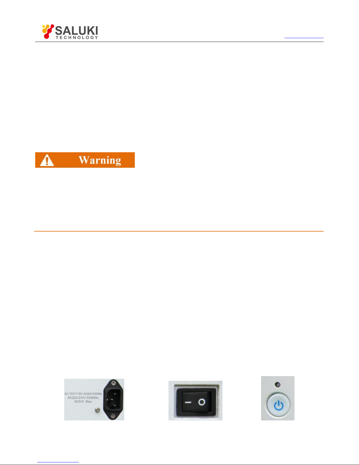
Step 1: connect the power line. Connect one end of the supporting power line of the network analyzer or the three-core power line
conforming to the requirements in the packing box to the power socket (as shown in Fig. 3.1) on the rear panel of the network analyzer.
The voltage indicator of the network analyzer is marked beside the power socket to remind the user that the applied voltage should
conform to the requirements. Connect the other end of the power cord to the required AC power supply.
Step 2: turn on the power switch on the rear panel. As shown in Fig. 3.2, check whether the standby indicator above the power switch on
the front panel (as shown in Fig. 3.3) is ON and yellow.
Step 3: turn on the power switch on the front panel, as shown in Fig. 3.3. Do not connect any device to the network analyzer before
start-up. Start the instrument under normal conditions. After start-up, the indicator above the power switch on the front panel will turn
green.
Fig. 3.1 S3602 Power Socket (Left)
Page 24
Tel: 886.2.2175 2930 Email: [email protected]
www.salukitec.com
24
Fig. 3.2 Switch on Rear Panel (Middle)
Fig. 3.3 Power Switch on Front Panel (Right)
b) Turn on/off
Start-up
Step 1: turn on the power switch (“|") on the rear panel.
Step 2: turn on the power switch in the lower left corner of the front panel. Check whether it is pressed ( ). In this case, the power
indicator above the power switch will turn green from yellow.
Step 3: about one minute is required for the network analyzer to start the Windows 7 system. After a series of self-inspection and
adjustment procedures, the main measurement program will be run.
Preheating for cold start of the instrument
In order to meet the performance indicators of S3602 series vector network analyzer in cold start, preheat it more than 30 minutes before
measurement.
Run the analyzer application program.
The application program will be automatically run after the network analyzer is started. After exiting the application program, you can run
the measurement program again according to the following method.
Method 1: click [Start] of the task bar in the lower left corner of the screen. Point to [Program] in the Start menu and then [Vector network
analyzer] in the program sub-menu. Click [Vector network analyzer] in the pop-up sub-menu. Then the measurement application program
will be run in the analyzer. You can also double-click the shortcut key on the desktop to run the program.
Method 2: press [Reset] in the functional key zone. Then the application program of the S3602 series vector network analyzer will be
run.
Shutdown
Step 1: turn off the power switch in the lower left corner of the front panel (as shown in Fig. 3.3). In this case, the shutdown process is
started (the power supply will be shut down after processing of software and hardware). After dozens of seconds, the instrument will be
powered off. The power indicator above the power switch will turn yellow from green.
Step 2: turn off the power switch ("O") on the rear panel, or disconnect the power supply of the instrument.
Thus the instrument is off.
Shut Down
The instrument in normal operation must be shut down by operating the power switch of the front panel. Do not directly operate the
power switch of the rear panel or directly cut off the power supply of the instrument; otherwise, the instrument cannot be shut down
normally and may be damaged, or the current status/measurement data may be lost. Shut down the instrument properly. In case of
failure of normal shutdown caused by the anomaly of the operating system or application program, hold [Power/Standby] key for four
seconds at least to shut down the analyzer.
Page 25

Tel: 886.2.2175 2930 Email: [email protected]
www.salukitec.com
25
c. Cutoff of power supply
In order to prevent personal injury under abnormal conditions, the power supply of the network analyzer requires emergency cutoff. In
this case, pull off the power cord (from the AC power socket or the power socket of the rear panel of the instrument). Therefore, sufficient
operating space should be reserved for direct cutoff of the power supply if necessary.
3.1.1.4.
Proper Use of Connector
The connector is always required in various tests of the network analyzer. Although the connectors of the calibrator, test cable and
analyzer measurement port are designed and manufactured according to the highest standards, the service life is limited. Inevitable wear
in normal operation may result in declining of performance indicators of the connector and failure to meet measurement requirements.
Proper connection of the connector in maintenance and measurement can help to obtain accurate and repeatable results, prolong the
service life of the connector, and reduce the measurement cost. Pay attention to the following items in actual operation.
1.Inspection of connector
Wear the anti-state wristband in connector inspection. It is recommended to use the magnifying lens to check the following items.
1) Check whether the plating surface is worn or deeply scratched.
2) Check whether threads are deformed.
3) Check whether there are metal particles on the connector threads and joint surfaces.
4) Check whether the internal conductor is bent or cracking.
5) Check whether the connector screw is tightened properly.
Prevent damage to the instrument port in connector inspection.
Any damaged connector may result in damage to the connector in good conditions even in the first measurement connection. In order to
protect each interface of the network analyzer, the connector must be checked before connection.
2.Cleaning of connector
Wear the anti-static wrist strap before cleaning the connector. Clean the connector according to the following steps.
1) Remove loose particles on the connector threads and joint plane with clean low-pressure air. Thoroughly check the connector. If
required, further clean the connector according to the following steps.
2) Soak the lint-free cotton swab with isopropyl alcohol (not thoroughly soaked).
3) Clean the dirt and debris on the joint plane and threads of the connector with the swab. Do not apply force on the internal conductor
at the center during cleaning of the internal surface. Do not leave the swab fibers on the central conductor of the connector.
4) Evaporate alcohol and purse the surface with compressed air.
5) Check the connector for particles and residues.
If the connector defect is still visible after cleaning, it indicates that the connector may be damaged and must not be used. Find the
causes of damage before measurement connection.
3.Connection method
Page 26
Tel: 886.2.2175 2930 Email: [email protected]
www.salukitec.com
26
Check and clean the connector before measurement connection. Ensure that the connector is clean and intact. Wea
the anti-static wristband in connection. The correct connection method and steps are as follows.
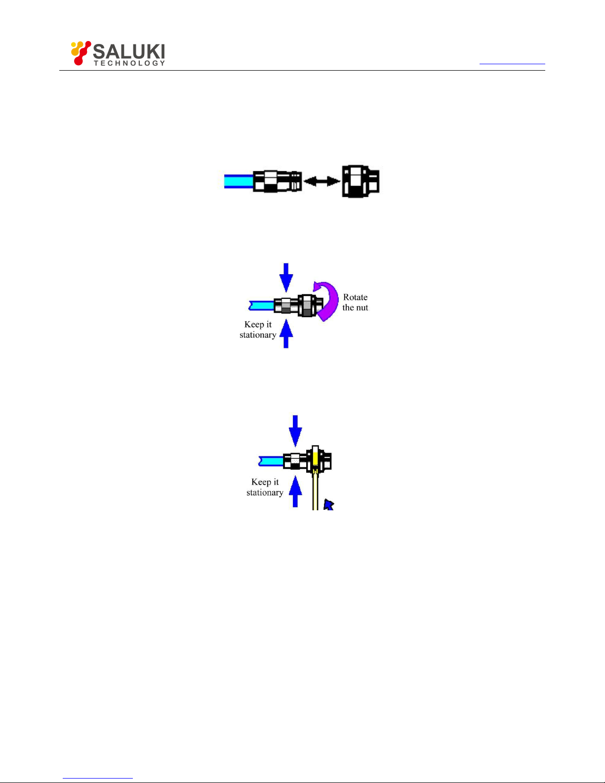
Step 1: as shown in Fig. 3.4, align the axes of two connectors to be interconnected, and ensure that the pin of the male connector can
concentrically slide into the jack of the female connector.
Fig. 3.4 Alignment of Axes of Interconnected Connectors
Step 2: as shown in Fig. 3.5, horizontally move two connectors to make them connected smoothly. Tighten the connector nut by means
of rotation (do not rotate the connector). Avoid relative rotation of connectors during connection.
Fig. 3.5 Connection Method
Step 3: as shown in Fig. 3.6, complete the final connection by tightening with the torque wrench. Note that the torque wrench must not be
beyond the initial break point. Use the auxiliary wrench to prevent the connectors from rotation.
Fig. 3.6 Final Connection with Torque Wrench
4.Disconnection method
Step 1: support the connectors to prevent any kind of force which may result in distortion, shaking or bending.
Step 2: use the open-end wrench to prevent the connector body from rotation.
Step 3: use another wrench to loosen the connector nut.
Step 4: rotate the connector nut by hand to complete final disconnection.
Step 5: horizontally separate two connectors.
5.Use of torque wrench
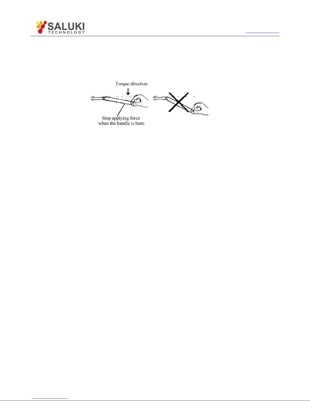
The use of the torque wrench is shown in Fig. 3.7. Pay attention to the following items.
Check whether the torque of the torque wrench is set properly before use.
Page 27
Tel: 886.2.2175 2930 Email: [email protected]
www.salukitec.com
27
Ensure that the angle between the torque wrench and the other wrench (used to support the connector or cable) is less than 90°
before applying force.
Carefully grip the handle end of the torque wrench, and apply force in the direction vertical to the handle to reach the break point of
the wrench.
Fig. 3.7 Use of Torque Wrench
6.Operation and storage of connectors
1) Connectors should be protected with covers if not in use.
2) Do not place various connectors, air lines and standard calibrators in one box in a messy manner. This is one of common causes of
connector damage.
3) Keep the connectors and analyzer at the same temperature. Hold and clean connectors with compressed air to greatly increase the
temperature. Do not calibrate the connectors until the temperature is stable.
4) Do not connect the joint planes of connectors. The skin oil and dust particles cannot be easily removed from joint planes.
5) Do not place the contact surfaces of connectors down to the hard table. Any contact with solid surfaces may cause damage to the
electric plating and joint planes of connectors.
6) Wear the anti-static wrist band and operate the instrument on the grounded conductive workbench mat to protect the analyzer and
connectors from the influence of static release.
7.Use of adapter
If the type of the measurement port of the analyzer is not applicable to the applied connector, use the adapter in measurement
connection. In addition, it is a good choice to use an adapter even if the connector type of the measurement port of the analyzer is the
same as that of the port of the tested device. The measurement port can be protected in these two cases, to prolong the service life and
reduce the maintenance costs. Carefully check and clean the adapter before connection to the measurement port of the analyzer. Use
the high-quality adapter to reduce the influence of mismatch on the measurement accuracy.
8.Joint plane of connector
One important concept of microwave measurement is a reference surface, which is the benchmark surface for all measurements of the
analyzer. The reference plane is defined as a joint plane of the measurement port and standard calibrator in the calibration process.
Good connection and calibration depends on the complete and smooth contact at all points of the joint planes of connectors.
Page 28

Tel: 886.2.2175 2930 Email: [email protected]
www.salukitec.com
28
Fig. 3.8 Calibration Plane
3.1.2.
System Recovery and Installation Program of Analyzer
Abnormal shutdown of software, infection of viruses or use of other kinds of software in the analyzer may result in anomaly of the
operating system of the analyzer. In this case, system recovery is recovered. Recover default settings of the analyzer according to the
following steps:
1) Shut down the analyzer and connect the keyboard to the USB interface.
2) Press the [Power/Standby] key in the lower left corner of the front panel of the analyzer. When the indicator of the external keyboard
is ON and the screen shown in Fig. 3.9 appears, immediately press [↑] and [↓], select "System Recovery", and press [Enter] of the
keyboard to automatically recover the system.
Fig. 3.9 Start-up Screen
Page 29
Tel: 886.2.2175 2930 Email: [email protected]
www.salukitec.com
29
Fig. 3.10 System Recovery Screen
3) If the screen shown in Fig. 3.10 appears, system recovery is started. About 10min is required in the whole process of system
recovery. Restart the analyzer after recovery.
3.1.3. Routine Maintenance
This section describes the routine maintenance of S3602 series vector network analyzers.
1) Cleaning of instrument surface
Clean the instrument surface according to the following steps:
Step 1: turn off the instrument by disconnecting the power line connected to the instrument.
Step 2: carefully wipe the surface with dry or slightly wet soft cloth. Do not wipe the inside of the instrument.
Step 3: do not use any chemical cleaner, such as alcohol, acetone or any cleaner which may be diluted.
2) Cleaning of display
Clean the display after a certain period of use. Follow the steps below:
Step 1: turn off the instrument by disconnecting the power line connected to the instrument.
Step 2: soak clean soft cloth with cleaner, and carefully wipe the display panel.
Step 3: dry the display with clean and soft cotton cloth.
Step 4: Connect the power line after the cleaner is thoroughly dry.
Page 30
Tel: 886.2.2175 2930 Email: [email protected]
www.salukitec.com
30
Clean the display.
There is anti-static coating on display surface, do not use fluoride-bearing detergent or acidic/alkaline detergent. Do not spray detergent
on display panel directly, otherwise it may penetrate into and damage the instrument
3.2.Front Panel & Rear Panel
This chapter introduces the elements and functions of the front panel, rear panel and operation interface of S3602 series vector network
analyzer.
Front panel
Rear panel
3.2.1.
Front Panel
This section introduces the structure and functions of the front panel of S3602 series vector network analyzer. The front panel is shown in
the following figure.
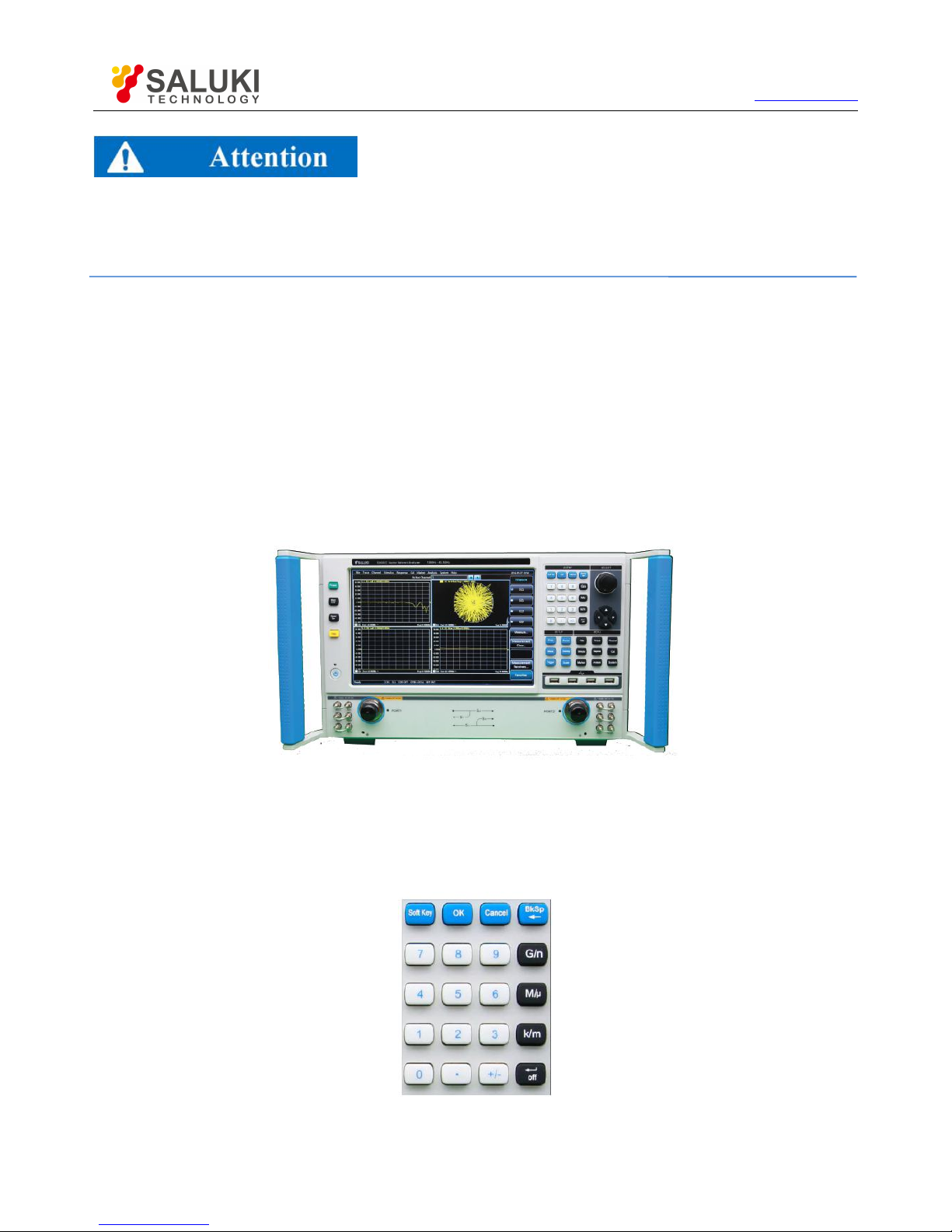
Fig. 3.11:Front Panel of S3602
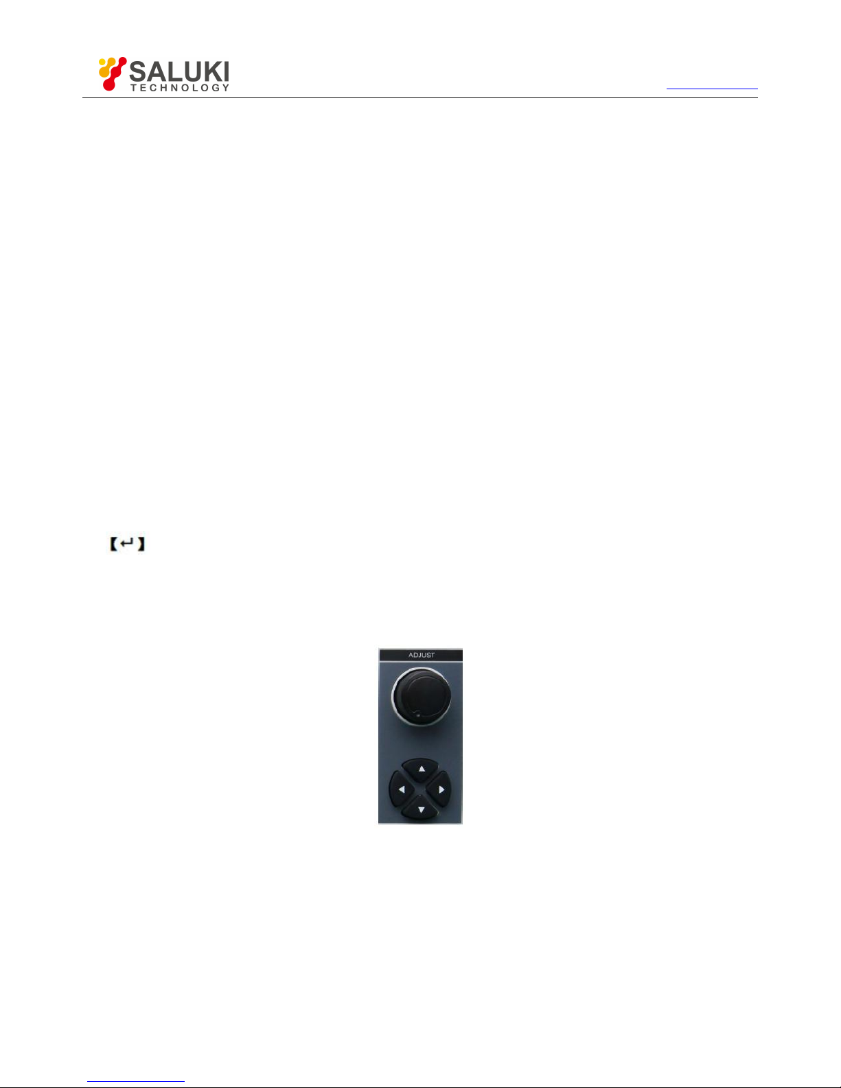
1.Input Key zone
The keys are used to enter measurement Setups, as shown in Fig 3.12.
Fig. 3.12 Input Key Zone of S3602
Page 31
Tel: 886.2.2175 2930 Email: [email protected]
www.salukitec.com
31
1) [OK] key
Confirm the Setups and input values in the dialog box and close the dialog box, equivalent to the "OK” button in the dialog box.
2) [Cancel] key
Ignore the Setups and input in the dialog box and close the dialog box, equivalent to the "Cancel” button in the dialog box.
3) [Soft Keyboard] key
Call the soft keyboard of the Windows 7 system.
4) [Backspace/←] key
Move the marker back and delete the original input after entering.
5) Number keys
Include 0-9. Enter the numbers in measurement Setup and press the corresponding unit keys to complete input.
6) Unit keys
End the number input and distribute a unit to each input value. The unit corresponding to each key is as follows:
[G/n]
G/ns (109/10-9)
[M/μ]
M/μs (106/10-6)
[k/m]
k/ms (103/10-3)
Basic units include dB, dBm, degree, second, Hz or dB/GHz. The keys can also be used to input values
with no unit and have the functions of the “Enter” key.
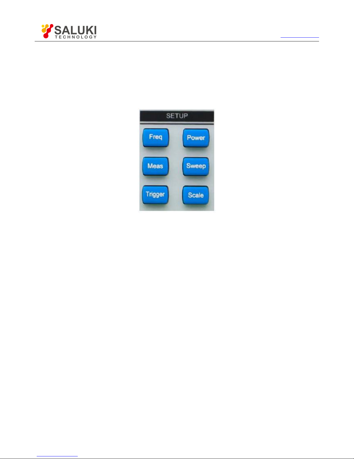
2.Adjustment key zone
Include navigation keys and knobs, as shown in Fig.3.13
Fig. 3.13 Adjustment Key Zone of S3602
1) Knob
Rotate the knob to adjust the set value in the current active input box.
2) [←] and [→] key
Move left or right to select the menu.
Switch the active options in the dialog box.
Page 32
Tel: 886.2.2175 2930 Email: [email protected]
www.salukitec.com
32
3) [↑] and [↓] key
Move up and down in the menu to select the menu item. When interact with dialog box, the arrow keys can be used to change value,
select item in the drop-down list, and select the desired option in a group of option list.
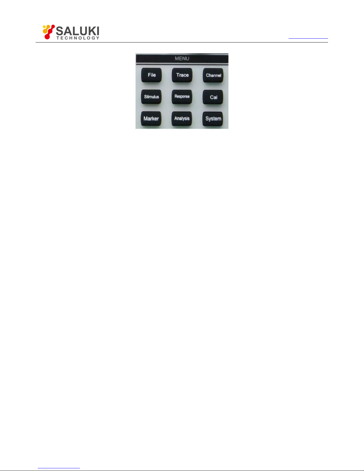
3.Setup key zone
Setup key zone include 6 Setup keys shown in Fig. 3.14.
Fig. 3.14: Setup Key Zone of S3602
1) [Freq] key
It is shortcut key to set the measurement frequency. The starting frequency, ending frequency, center frequency, frequency span and
frequency offset.
2) [Power] key
It is a shortcut key to set the measurement power. The power level, power status ON/OFF, power attenuation and power slope.
3) [Measurement Setup] key
It is a shortcut key to measurement Setups. For Measurement Setup Details, please refer to section 4.2
4) [Sweep Setup]key
It is a shortcut key to sweep Setups. For Sweep Setup Details, please refer to section 4.5
5) [Trigger Mode] key
It is a shortcut key to Trigger mode. For trigger mode Details, please refer to section 4.6
6) [Scale Setup] key
It is a shortcut key to scale Setups. For scale Setup Details, please refer to section 4.7
4.Menu key zone
Menu key zone include 9 menu keys shown in Fig. 3.15.
Page 33
Tel: 886.2.2175 2930 Email: [email protected]
www.salukitec.com
33
Fig.3.15: Menu Key Zone of S3602
1) [File] key
Open the main file menu. Following options will be displayed on screen: “Save”, “Call”, “Print”, “Minimize application program” and “Exit”.
2) [Trace] key
Open the main Trace menu. Following options will be displayed on screen: “New Trace”, “Delete Trace”, “Select Trace”, “Move Trace”,
“Trace title” and “Maximize Trace”.
3) [Channel] key
Open the main channel menu and the current channel will be selected automatically. Following options will be displayed on screen:
“Channel 1/2/3/4”, “Open channel”, “Close channel”, “Select channel”, “Copy channel” and “Hardware Setup”.
4) [Stimulus] key
Open the main Stimulus menu. Following options will be displayed on screen: “Frequency”, “Power”, “Sweep” and “Trigger”.
5) [Response] key
Open the main response menu. Following options will be displayed on screen: “Measurement”, “Format”, “Scale”, “Display” and
“Average”.
6) [Calibration] key
Open the main calibration menu. Following options will be displayed on screen: “Calibration”, “Correction ON/OFF”, “Interpolation
ON/OFF”, “Port extension”, “Fixture”, “Edit calibrator”, “Attribute” and “Power calibration”.
7) [marker] key
Open the main marker menu. Following options will be displayed on screen: “marker”, “marker function”, “marker search”, “marker
attribute” and “marker display”. If no marker is enabled at present, the marker 1 will be enabled automatically in the default mode. If a
marker is enabled, the current marker will be selected automatically.
8) [Analysis] key
Open the main analysis menu. Following options will be displayed on screen: “Save”, “Test”, “Trace statistics”, “Gate”, “Window”, “Time
domain”, “Structural return loss” and “Formula editor”.
9) [System] key
Open the main system menu. Following options will be displayed on screen: “Configuration”, “Record/Run”, “Spread spectrum”,
“Windows task bar”, “Reset”, “Custom user reset state” and “Language”.
Page 34
Tel: 886.2.2175 2930 Email: [email protected]
www.salukitec.com
34
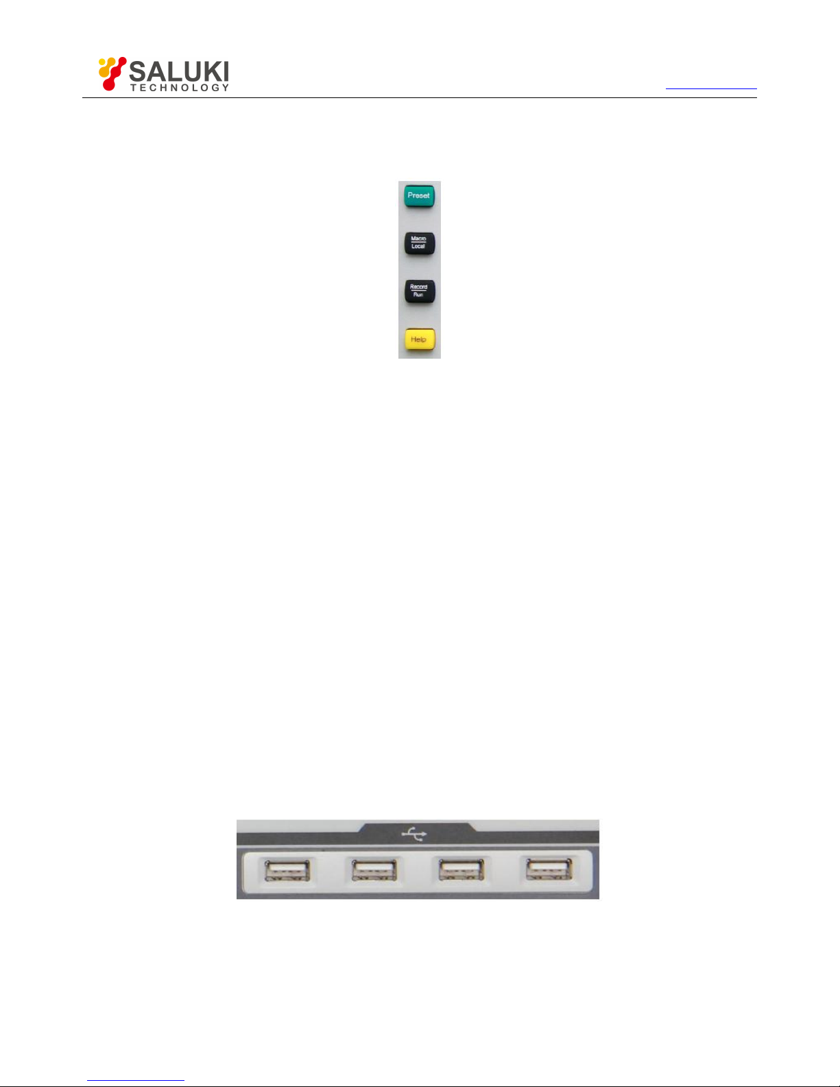
5.Function Key Zone
Function key zone include 4 function keys on the left side of the screen as shown in Fig. 3.16.
Fig. 3.16: Function Key Zone of S3602
1) [Help] key
Open the main help menu. Following options will be displayed on screen: “User manual”, “Programming manual”, “Technical support”,
“Error information” and “About”.
2) [Record/run] key
It is a shortcut key to enable the recording/running function of the analyzer. Press the key to automatically start recording. If recording is
completed, press this key to automatically start running. This key is only effective for Record/Run 1, and cannot be used to control
Record/Run 2.
3) [Macro/local] key
If the analyzer is programmed, press this key to switch to the macro state. If the analyzer is not programmed, press this key to open the
macro menu.
4) [Preset]key
It is a shortcut key to reset the analyzer. If the user has saved the reset state and tick the item “Enable user reset state”, press this key
to recover the state saved by the user; otherwise, the system reset state will be recovered.
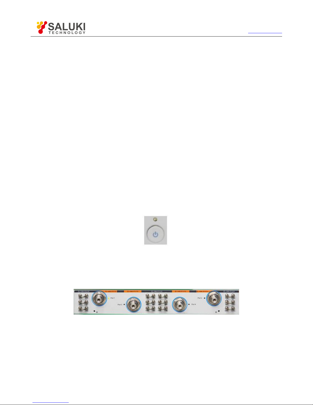
6.USB Interface
The USB interface can be connected with the keyboard, mouse and other USB devices. The front panel is equipped with four USB
interfaces in total and conforms to the USB2.0 specifications. The interface jack is of A type (four embedded contacts; Contact 1 on the
left side).
Fig. 3.17: USB Interface
7.Display screen
Page 35
Tel: 886.2.2175 2930 Email: [email protected]
www.salukitec.com
35
The display screen of the analyzer is a TFT LCD screen. Technical indicators are as follows:
12.1-inch touch screen
Resolution: 1280×800
Vertical refresh rate: 60Hz
Horizontal refresh rate: 48.4Hz
8.[Start/Standby] key and indicator
The [Start/Standby] key and indicator are shown in Fig. 3.18. The power switch is used to start the analyzer or enable the standby state
of the analyzer.
The indicator is green when the analyzer is started.
The indicator is orange when the analyzer is in the standby state.
Press the power button to start the analyzer. Then the Windows 7 operating system will be run automatically and the measurement
application program will be loaded.
When the power button is pressed in the standby state, the analyzer will automatically exit the application program. When the
power supply will be turned off, the standby state will be enabled.
This is only a standby switch. It cannot be directly connected with the external power supply or used to cut off the connection
between the instrument and external power supply. The external power supply of the analyzer can be shut down by the power
switch on the rear panel. The connection between the analyzer and external power supply can be fully cut off by removing the
power cable.
Fig. 3.18: [Start/Standby] Key and Indicator
9.Test port
As shown in Fig. 3.19, the instrument is equipped with 2x 50Ω ports and 2x 3.5mm/2.4mm/1.85mm ports (male). The instrument can act
as both RF source and receiver. so as to measure the tested device in bi-directions. The yellow light indicates the source output port.
Fig. 3.19: Test Ports of Analyzer
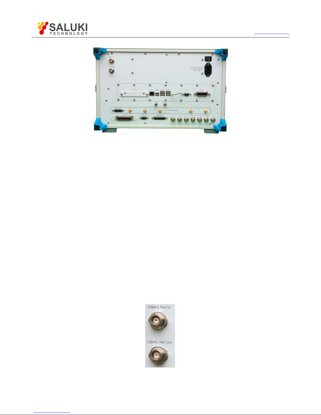
3.2.2. Rear Panel
This section introduces the structure and functions of the rear panel of S3602 series vector network analyzer. The rear panel is shown in
the following figure.
Page 36
Tel: 886.2.2175 2930 Email: [email protected]
www.salukitec.com
36
Fig. 3.20: Rear Panel of Network Analyzer
1.10MHz reference connector
1) 10MHZ reference output
As shown in Fig. 3.21, the BNC (female) connector can be used for connection between the analyzer and external reference signal. The
10MHZ external reference signal detected by the port will be used as the reference frequency of the instrument, instead of the internal
reference frequency. The 10MHz reference input port has the following features:
Input frequency: 10MHz±1ppm
Input level: -15dBm to +20dBm
Input impedance: 200Ω
2) 10MHZ reference output
The reference signal with the following features can be provided for the outside through the BNC (female) connector.
Output frequency: 10MHz±1ppm
Signal type: sine wave
Output level: 13dBm±4dB into 50Ω
Output impedance: 50 Ω
Fig.3.21: 10MHz Reference Connector
Page 37
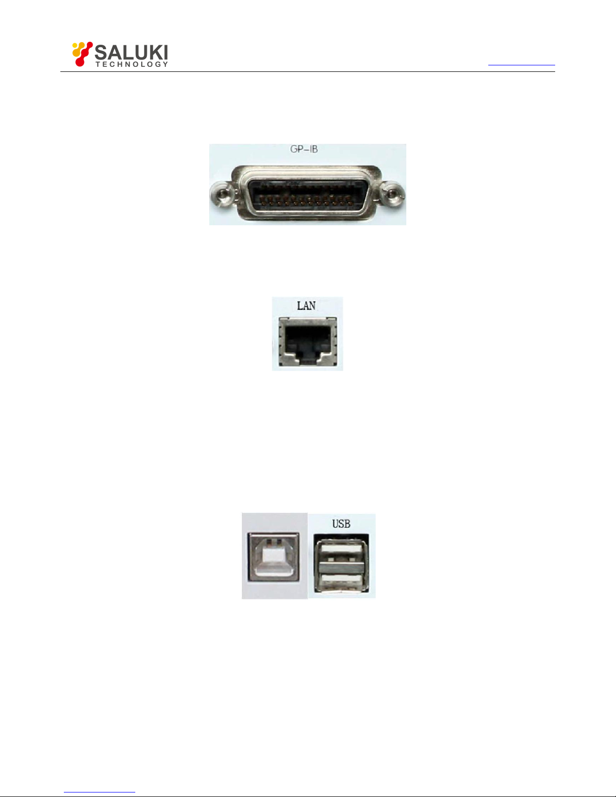
Tel: 886.2.2175 2930 Email: [email protected]
www.salukitec.com
37
2.General-interface bus connector
As shown in Fig.3.22 this is a 24-pin D-type female connector, meeting the IEEE-488 standards. It is used to transmit and receive
GPIB/SCPI commands.
Fig. 3.22: General-interface Bus Connector
3.LAN connector
As shown in Fig. 3.23, this is a 10/100/1000BaseT Ethernet connector of standard 8-pin structure, and three data rates can be selected.
Fig. 3.23: LAN Connector
4.USB connector
As shown in Fig. 3.24, the connector jack is of Type A (four embedded contacts; with Contact 1 on the left side) and Type B. Type A
connector can be connected to the USB mouse, keyboard or other USB interface devices. The rear panel is equipped with four interfaces
in total.
Type B connector is mainly used for control. The network analyzer can be connected to the external computer or remote device through
SCPI control. The rear panel is equipped with one interface.
Fig. 3.24: USB Connector (B-type on the left and A-type on the right)
5.Video graphic adapter (VGA) output connector
As shown in Fig. 3.25, this is a 15-pin D-sub female connector to be connected with the external VGA display of corresponding resolution.
In this case, the user can observe the internal and external display at the same time.
Page 38
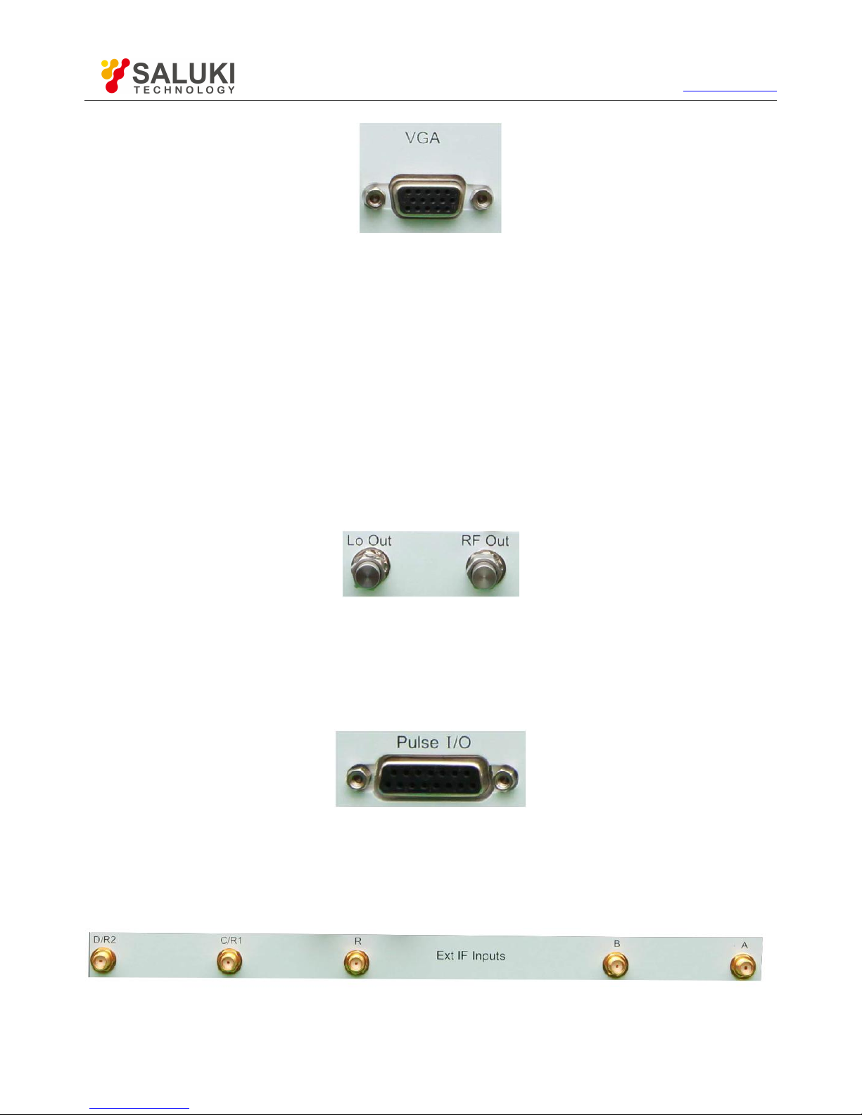
Tel: 886.2.2175 2930 Email: [email protected]
www.salukitec.com
38
Fig. 3.25: VGA Connector
6.LO and RF output connector
As shown in Fig. 3.26, the 3.5mm female interface is used for LO output and RF output. The LO interface is used for internal LO signal
output, and RF interface for RF source signal output. The connector can be used for fault detection and millimeter wave spreading. The
interface features are as follows:
Frequency range of LO output signal:
12.535MHz-13.507606GHz/26.507606GHz/43.507606GHz/50.007606GHz/67.007606GHz
Power range of LO output signal: -4dBm to 6dBm
Frequency range of RF output signal: 3.2GHz-13.5GHz/26.5GHz/43.5GHz/50GHz/67GHz
RF output signal power: -3dBm±2dB
Fig. 3.26: LO and RF Output Connector
7.Pulse input/output connector
As shown in Fig. 3.27, this is a 15-pin D-type female connector. The working status of the internal pulse generator can be monitored
synchronously through this interface.
Fig. 3.27: Pulse Input/Output Connector
8.External IF input connector
As shown in Fig. 3.28, five SMA interfaces are used for external IF input of the vector network. The two-port model is marked with A, B,
R1 and R2, and the four-port with A, B, C, D and R.
Fig. 3.28: Intermediate Input Connector
Page 39
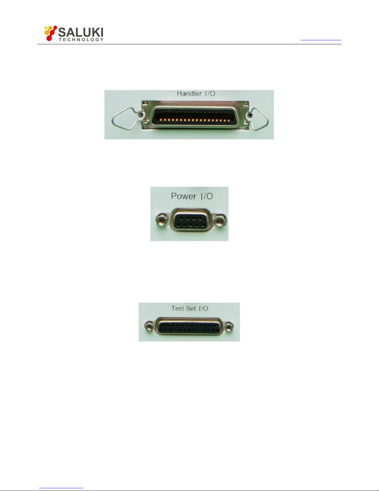
Tel: 886.2.2175 2930 Email: [email protected]
www.salukitec.com
39
9.Automatic test interface connector
As shown in Fig. 3.29, this interface is a 36-pin female connector. The network analyzer and material handler can exchange signals
through this interface to provide a stable and reliable automatic test environment for the user.
Fig. 3.29: Automatic Test Interface Connector
10.Extension interface connector
As shown in Fig. 3.30, this interface is a 9-pin D-type female connector.
Fig. 3.30: Extension Interface Connector
11.External tester interface connector
As shown in Fig. 3.31, this tester interface is a DB-25 female interface, including 13 addresses and data multiplexing lines, three control
lines and one interruption control line, and is used to control the external tester (such as the external spread spectrum controller).
Fig. 3.31: External Tester Interface Connector
12.Trigger input/output interface connector
As shown in Fig. 3.32, this interface is an external and auxiliary trigger input/output interface. Specific functions are as follows:
External trigger input - if it is enabled, the vector network analyzer will be triggered according to the connected signal.
External trigger ready - if it is enabled, the vector network analyzer will send a “Ready” signal to the external device through this
interface.
Auxiliary trigger input 1/2 - if it is enabled, the external device will send an “OK” signal (meaning the external device is ready to
receive trigger signal) to the vector network analyzer through this interface.
Auxiliary trigger output 1/2 - if it is enabled, the vector network analyzer will send an “OK” signal through this interface before (or
Page 40
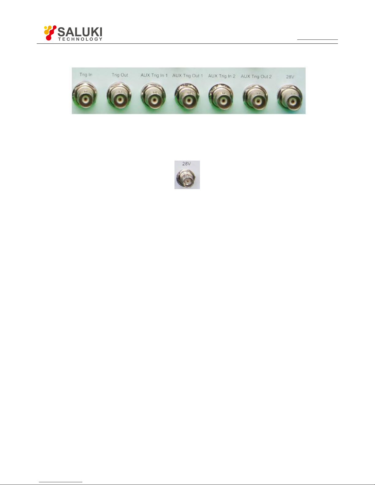
Tel: 886.2.2175 2930 Email: [email protected]
www.salukitec.com
40
after) one measurement.
Fig.3.32: Trigger Input/Output Interface Connector
13.28V (BNC) interface connector
As shown in Fig. 3.33, this BNC (female) connector can be used to drive a noise source.
Fig.3.33: 28V (DC) Interface Connector
Page 41
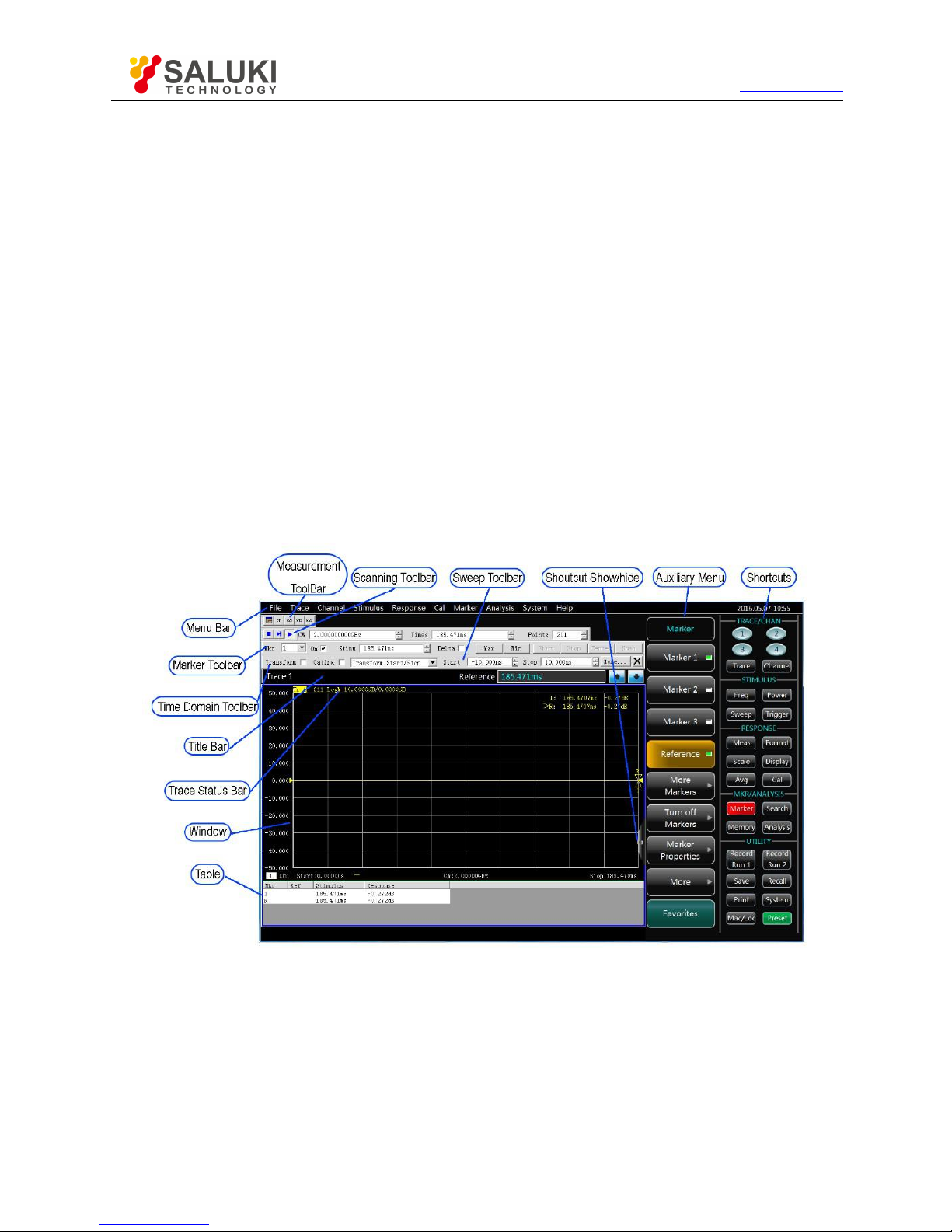
Tel: 886.2.2175 2930 Email: [email protected]
www.salukitec.com
41
3.3.
Graphic User Interface
As shown in Fig. 3.34, the mouse can be used to realize the following operations.
Click the menu bar to display the drop-down menu.
Click the input toolbar to adjust the entered number.
Click the marker toolbar to use the marker.
Click the measurement toolbar to add the measurement trace.
Click the sweep toolbar to control sweep of the analyzer.
Click the stimulus toolbar to set sweep stimulus.
Click the time domain toolbar to set time domain settings.
Right-click the mouse on the screen to display the right-click menu.
Click the trace bar to select the current activation trace.
Right-click the mouse on the trace bar to set the current activation trace in the right-click menu.
Click the auxiliary menu bar and shortcut toolbar to perform corresponding settings.
Fig. 3.34 Display Screen of Analyzer
Page 42

Tel: 886.2.2175 2930 Email: [email protected]
www.salukitec.com
42
3.4.
Trace, Channel and Window of Analyzer
Trace
Channel
Window
3.4.1. Trace
The trace is a series of measurement data points. Trace settings will affect the mathematical operation and display of measurement
data. Only the settings of the active trace can be changed. Click the corresponding trace status button to active the trace. For
detailed setting, refer to "change trace activation status" of "4.2 Selection of Measurement Parameter". Trace settings include:
Measured parameters
Display format
Scale
Trace operation
Marker
Electrical delay
phase offset
Smoothing
Time domain transformation
3.4.2. Channel
The channel is a trace container. The analyzer supports 64 channels in total. Channel settings are associated with measurement of
the trace in the channel. The same channel settings are applicable to tracks in the same channel. Only the settings of the active
channel can be changed. Once the trace in the channel is activated, the channel will also be activated. For detailed settings of the
active trace, refer to "change trace activation status" of "4.2 Selection of Measurement Parameter".Channel settings include:
Frequency span
Power
Standard data
Intermediate-frequency bandwidth
Number of sweep points
Sweep setting
Average
Trigger (for some settings)
3.4.3. Window
The window is used to observe the measurement trace. The analyzer supports 32 windows at most, and eight tracks can be
displayed at most in each window. Set the window display by the [View] menu. For details, refer to "4.9 Setting of Analyzer Display".
1.Create a new window.
Menu path: [Response] > [Display] > [Window] > [New window]. Then a new window will be created. The default setting of the trace
in the window is S11, indicating Channel 1.
Page 43
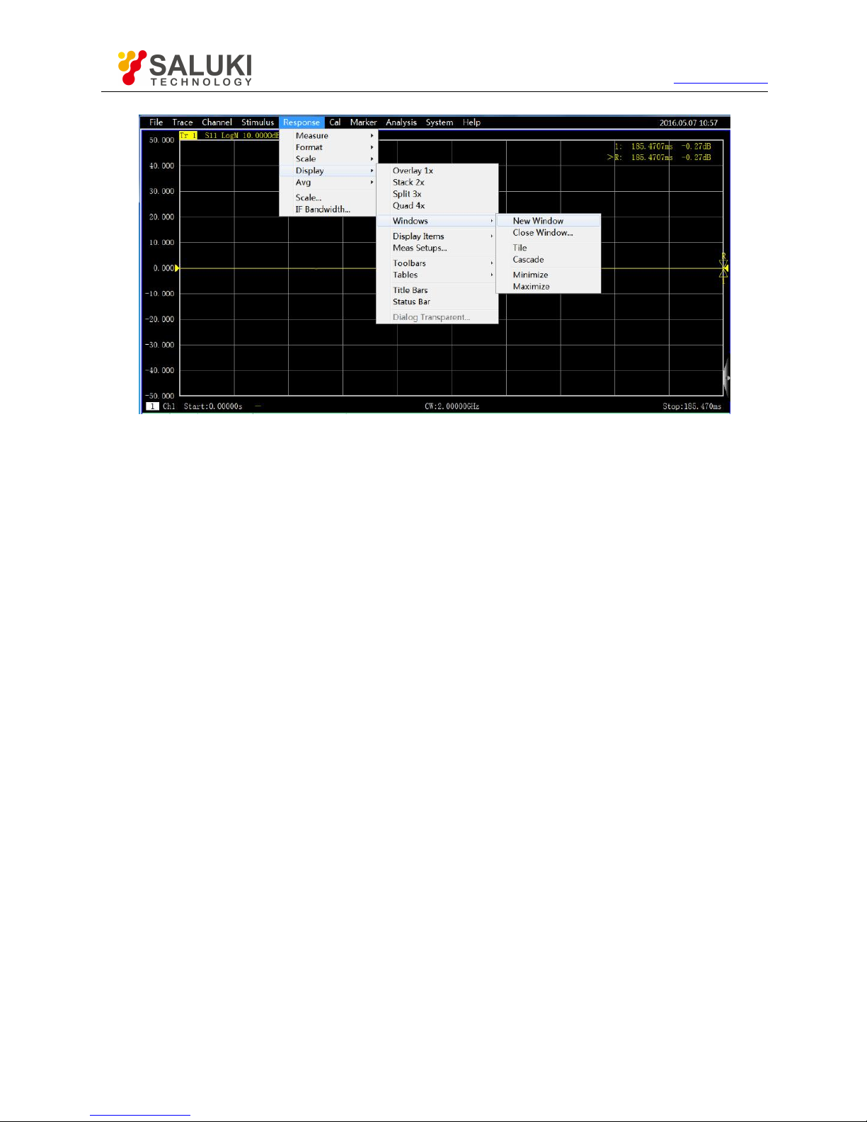
Tel: 886.2.2175 2930 Email: [email protected]
www.salukitec.com
43
Fig. 3.35 Creation of New Window
2.Use the full screen window.
If several windows are opened at the same time, the trace will be unclear as a result of too small window size. In this case, one
window can be displayed in the full screen so as to better observe the trace in the window.
Use the mouse to display one window in the full screen according to the following three methods.
If the title bar is opened, click the "Maximize" button in the title bar of the window.
If the title bar is closed, double-click the mouse in the window to be maximized.
Menu path: [Display] > [Window] > [Maximize].
Page 44
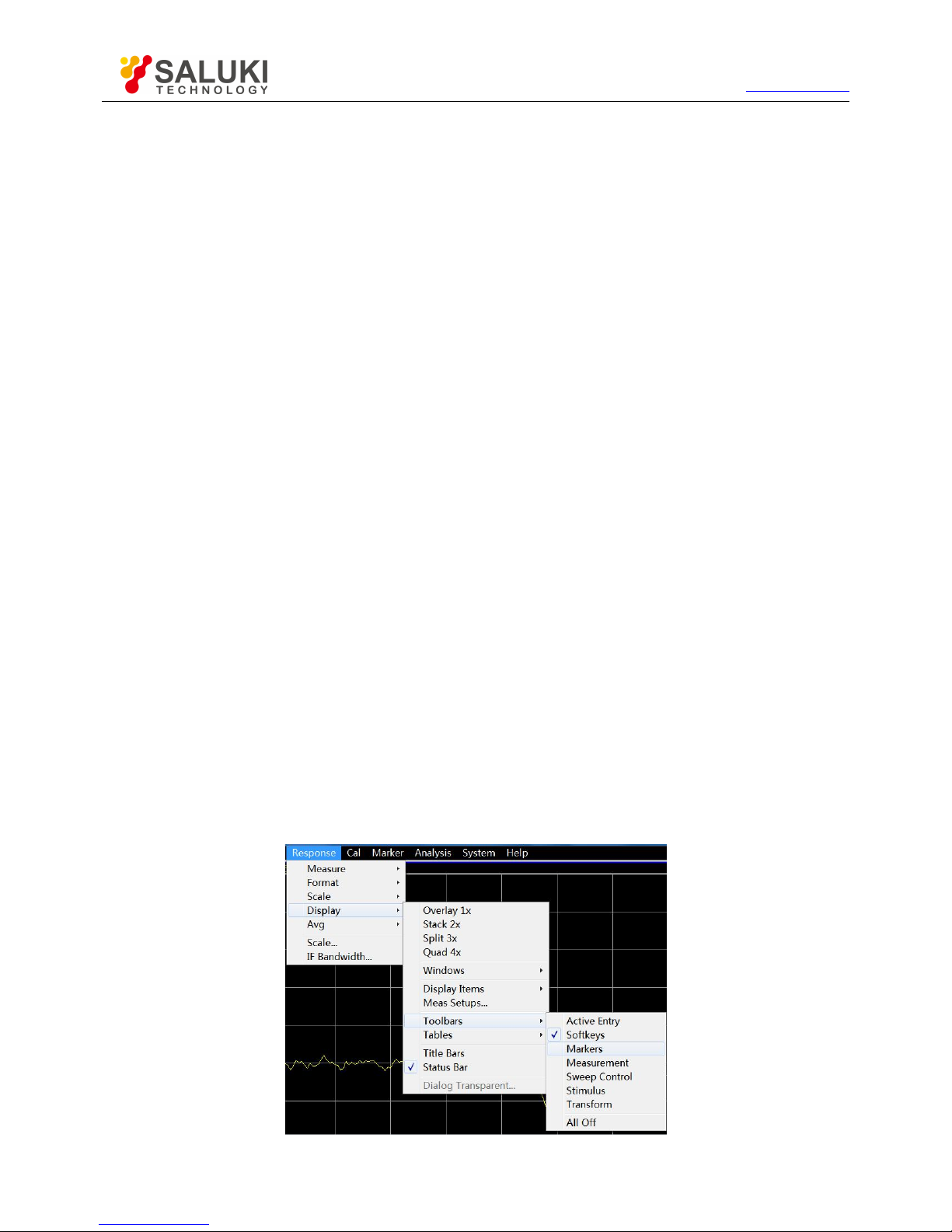
Tel: 886.2.2175 2930 Email: [email protected]
www.salukitec.com
44
3.5.
Data Analysis
Marker
Trace operation and statistics
Limit test
Ripple test
Bandwidth test
Equation Editor
3.5.1.
Marker
Use the marker to read the measurement data, search the values of specific type or change the excitation settings. Nine normal
marker and one reference marker can be used at most for each trace.
Equation Editor
Move marker
Marker search
Marker function
Advanced marker option setting
Marker list
3.5.1.1. Create marker
1.Use of marker functions
1) Marker toolbar
Menu path: [Response] > [Display] > [Toolbar]. Click [Marker] in the toolbar sub-menu to display the marker toolbar.
Select the marker to be opened in the [Marker] box.
Set the marker stimulus value in the [Stimulus] box.
Click the [Open] check box.
Fig. 3.36 Creation of marker by marker Toolbar
Page 45
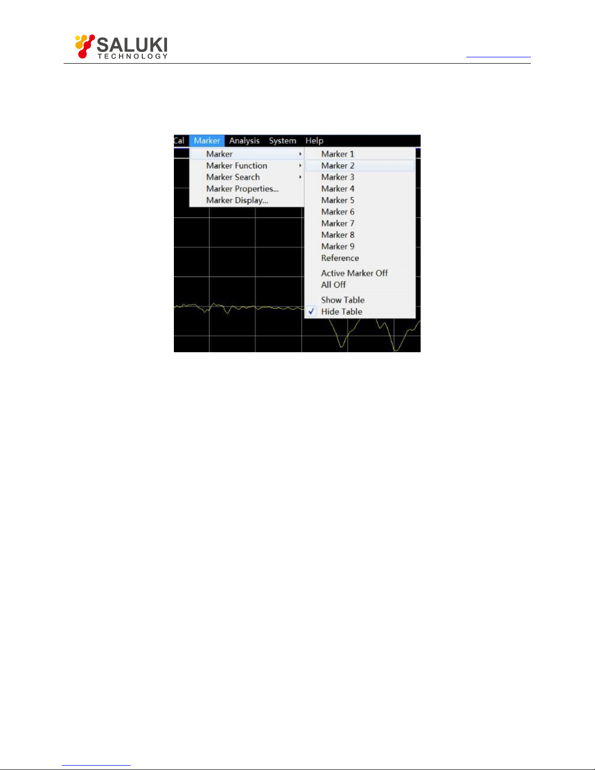
Tel: 886.2.2175 2930 Email: [email protected]
www.salukitec.com
45
2) Marker menu
Menu path: [Marker] > [Marker]. The marker sub-menu will be displayed.
Click the marker to be opened in the sub-menu.
Fig. 3.37 Creation of marker by marker Menu
3) Marker dialog box
Menu path: [Marker] > [Marker] > [Marker...]. The marker dialog box will be displayed.
Select the marker to be opened in the [Marker] box.
Set the marker Stimulus value in the [Stimulus] box.
Click the [Open] check box.
4) Marker dialog box
a. [Marker] box
Select the marker to be defined.
b. [Stimulate] box
Define the stimulate value of X-axis of the selected marker.
c. [Open] check box
Select it to open the marker in the marker dialog box and clear it to close the marker in the marker dialog box.
d. [△ marker] check box
Select it to display the relative values of the selected marker and reference R marker. If the marker R is not
opened, select the check box to automatically open the reference R marker.
e. [Advanced marker...] button
Click it to display the advanced marker dialog box.
f. [Close all markers] button
Page 46
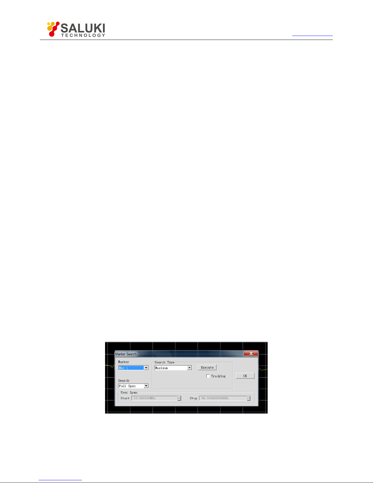
Tel: 886.2.2175 2930 Email: [email protected]
www.salukitec.com
46
Click it to close all the opened marker.
3.5.1.2. Move marker
1) Activate the marker to be moved in one of the above three methods.
2) Move the marker in one of the following methods.
a. Click the [Stimulate] box in the marker dialog box and move the marker in the following method.
Directly enter the marker stimulate value.
Rotate the knob to move the marker.
Click the [↑] or [↓] in the [Stimulate] box to change the marker stimulate value.
Press [↑] or [↓] in the adjustment key zone to change the marker stimulate value.
b. Click the [Stimulate] box in the marker toolbar and move the marker in the following method.
Directly enter the stimulus value.
Rotate the knob to move the marker.
Click the [↑] or [↓] in the [Stimulate] box to change the marker stimulate value.
Press [↑] or [↓] in the adjustment key zone to change the marker stimulate value.
c. Move the marker in the input toolbar in the following method.
Directly enter the stimulate value.
Rotate the knob to change the stimulate value.
Press [↑] or [↓] in the adjustment key zone to change the marker stimulate value.
click the Up and Down arrow in the input box to change the marker stimulate value.
3.5.1.3. Marker search
Search the specific measured value with the marker searching function. If no matching measurement data are found, the marker will
remain unchanged in the current position.
1) Marker search method:
Menu path: [Marker] > [Marker search].
Set the marker search in the dialog box. Click [Execute] to execute marker search and [OK] to close the dialog box.
Fig. 3.38 Marker Search
2) Marker search dialog box
a. Marker zone
Page 47
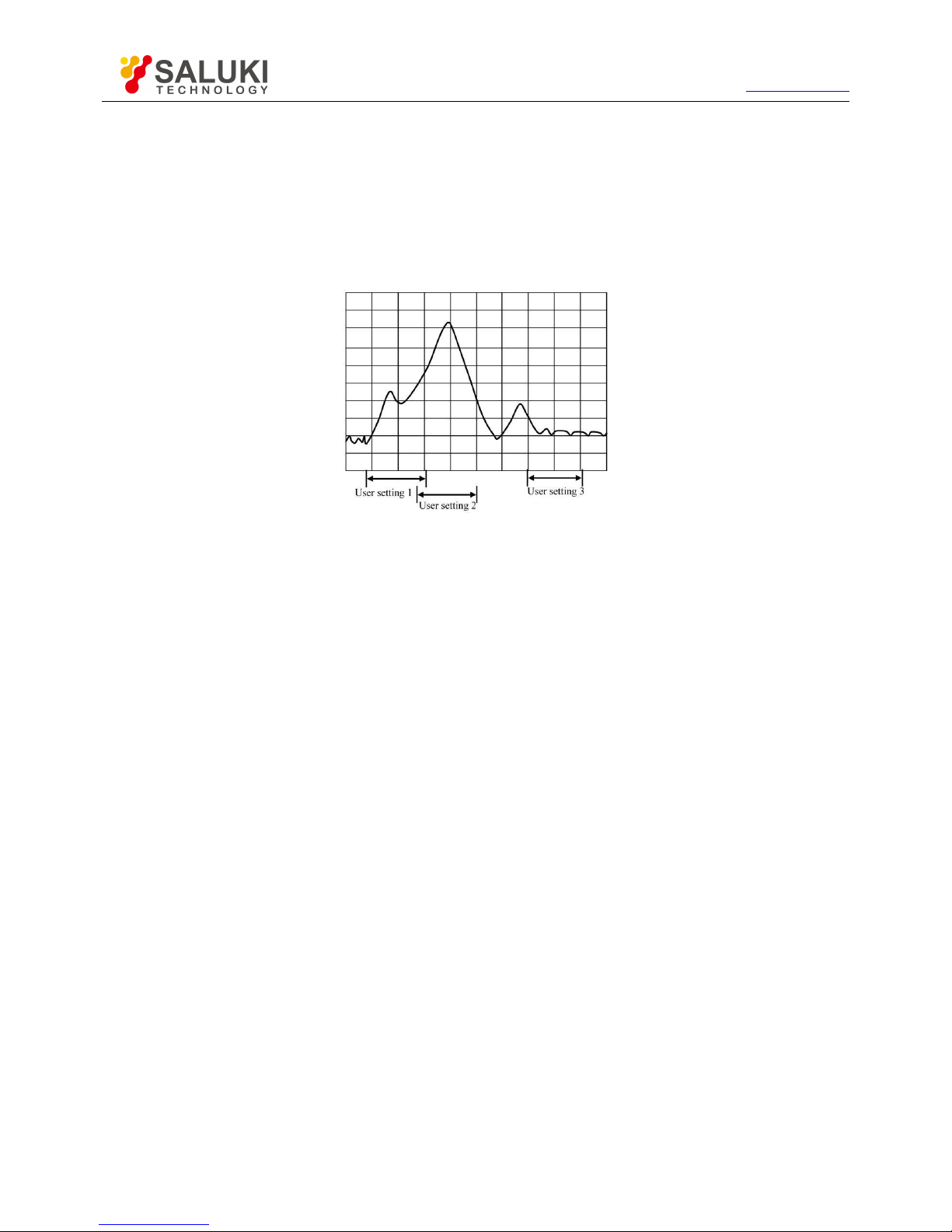
Tel: 886.2.2175 2930 Email: [email protected]
www.salukitec.com
47
Select the marker to be defined for search.
b.Search domain zone
Define the range of marker search. The default search domain is the full bandwidth. In addition, the instrument supports the search of
nine user settings. The user setting to be selected must be defined in the user domain range. The ranges of search domains set by
users are allowed to be overlapping. Various marker can be applied in one search domain. Fig. 3.39 shows a group of search domains
set by users.
Fig. 3.39 Schematic Diagram of Search Domains Set by Marker Users
c.User domain range zone
The [Start] box and [End] box within the User domain range zone are used to define the search domain set by the user.
d.Search type zone
Define the type of marker search. The analyzer supports the following 10 search types:
Minimum value: search the minimum measurement data point.
Maximum value: search the maximum measurement data point.
Right peak value: search next effective peak value on the right side of the marker. The peak must be defined at first.
The peak is defined according to [Threshold] and [Offset]. The minimum peak point is defined in the [Threshold] box. The effective
peak point must be above the threshold value, and the valley points on both sides may be less than the threshold value. The minimum
vertical distance between the peak value and valley value is defined in the [Offset] box. The vertical distance between the effective
peak value and valley values on both sides must be more than the offset value. The analyzer settings in Fig. 3.40 are as follows:
Threshold: -50dB
Offset: 10dB
Scale: 10dB/grid
1) Peak A is effective, and the threshold and peak value conform to the requirements.
2) Peak B is not effective, and the offset does not conform to the requirements.
3) Peak C is not effective, and the threshold does not conform to the requirements.
Page 48
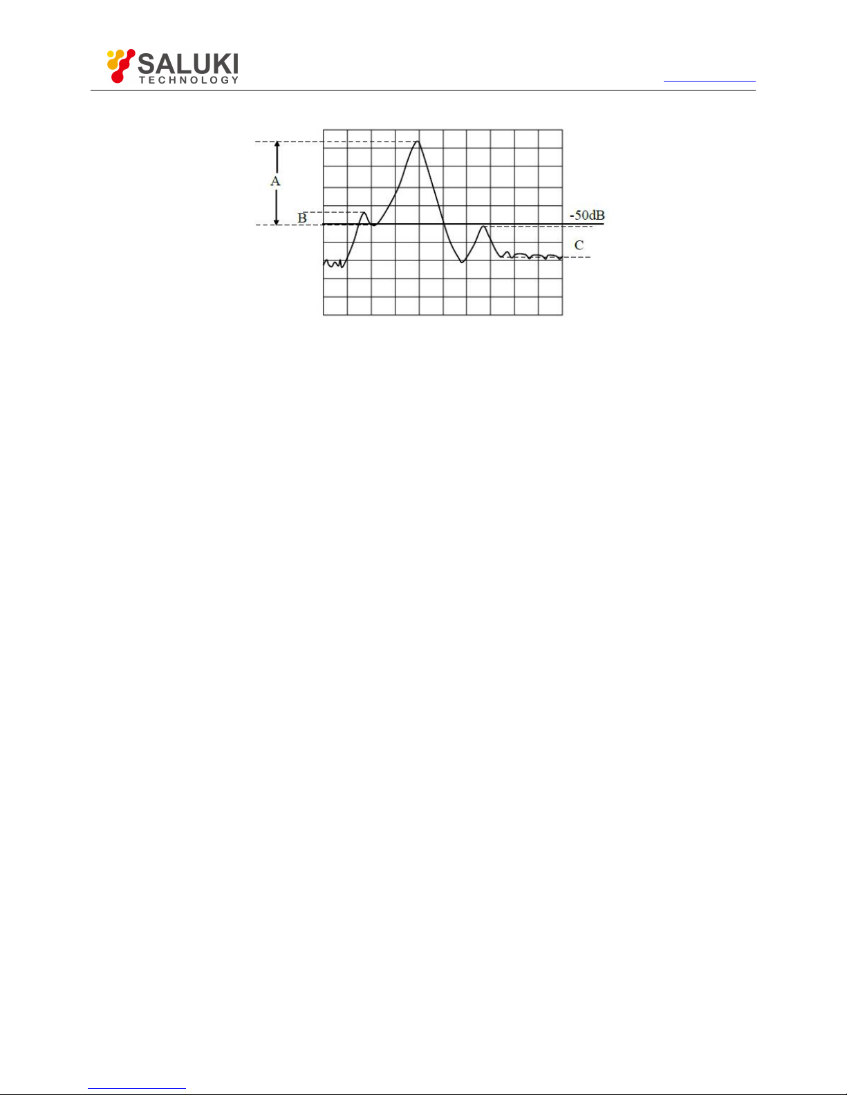
Tel: 886.2.2175 2930 Email: [email protected]
www.salukitec.com
48
Fig. 3.40 Schematic Diagram of Peak in marker Domain
Left peak: search next effective peak value on the left side of the marker. The peak must be defined at first.
Next peak: search next peak lower than the current marker amplitude. The peak must be defined at first.
Target: enter the search target value in the [Log] box and click [Execute]. The marker will move to the first target value on the
right side of the current marker location. Then continuously click [Execute], and the marker will move to next target value on the
right side until it reaches the maximum stimulus value. In this case, the marker will return to the lowest stimulus value to search
the target value.
If the [Discrete marker] is selected in the [Advanced marker] dialog box, the marker will move to the discrete data point
corresponding to the target value.
If the [Discrete marker] is cleared in the [Advanced marker] dialog box, the marker will move to the interpolation data point
corresponding to the target value.
Left target: only search the target value on the left side of the current marker.
Right target: only search the target value on the right side of the current marker.
Bandwidth: if the bandwidth searching function is selected, set the level (default: -3dB) below the peak in the level box and
measure the bandwidth at the set level, as shown in Fig. 3.41. Use marker 1-4 for measurement. marker 1 is used to search the
maximum peak value, marker 2 to search the point of specified level on the left side of the peak, marker 3 to search the point of
specified level on the right side of the peak, and marker 4 to search the center of the bandwidth. The following information will be
displayed after measurement.
Bandwidth: frequency difference between the right and left cutoff frequency point.
Center: frequency of the middle point between the right and left cutoff frequency point.
Q: value calculated by dividing the center frequency by the bandwidth.
Loss: value measured at the center frequency point of the bandwidth.
Left cutoff: minimum frequency of two points below the specific bandwidth level of the signal peak.
Right cutoff: maximum frequency of two points below the specific bandwidth level of the signal peak.
Page 49
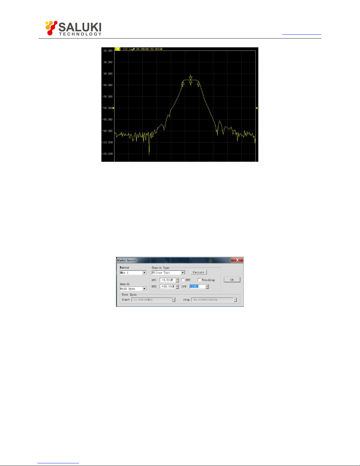
Tel: 886.2.2175 2930 Email: [email protected]
www.salukitec.com
49
Fig. 3.41 Bandwidth Search
Filter test: the analyzer has a special shortcut function to test the filter, and all test parameters will be automatically displayed on
the screen so that the user can directly observe measurement results. As manual setting in the test is eliminated, the speed of
filter test is greatly increased. As shown in Fig. 3.42.
Eight parameters of the filter test are displayed in the upper left corner of the trace. When the filter test is started, bandwidth search
will be automatically enabled, and six parameters of the bandwidth test will be displayed in the upper right corner at the same time.
Level of Bandwidth 1: set the level of Bandwidth 1 in the input box.
Level of Bandwidth 2: set the level of Bandwidth 2 in the input box.
Percentage frequency offset: set the percentage of frequency offset in the input box.
Fig. 3.42 Filter Test
a) [Execute] button
Click the [Execute] button to execute one marker search of specified type.
b) [Tracking] check box
If [Tracking] is selected, the search function will be executed after each sweep according to the current search type and domain
setting. In this case, the marker will be in the desired position after each sweep.
3.5.1.4. Marker function
1.Use of marker functions
Some settings of the instrument can be changed according to the marker activation position, such as the starting frequency, ending
frequency, etc. The setting method is as follows.
Menu path: [Marker] > [Marker function].
Page 50
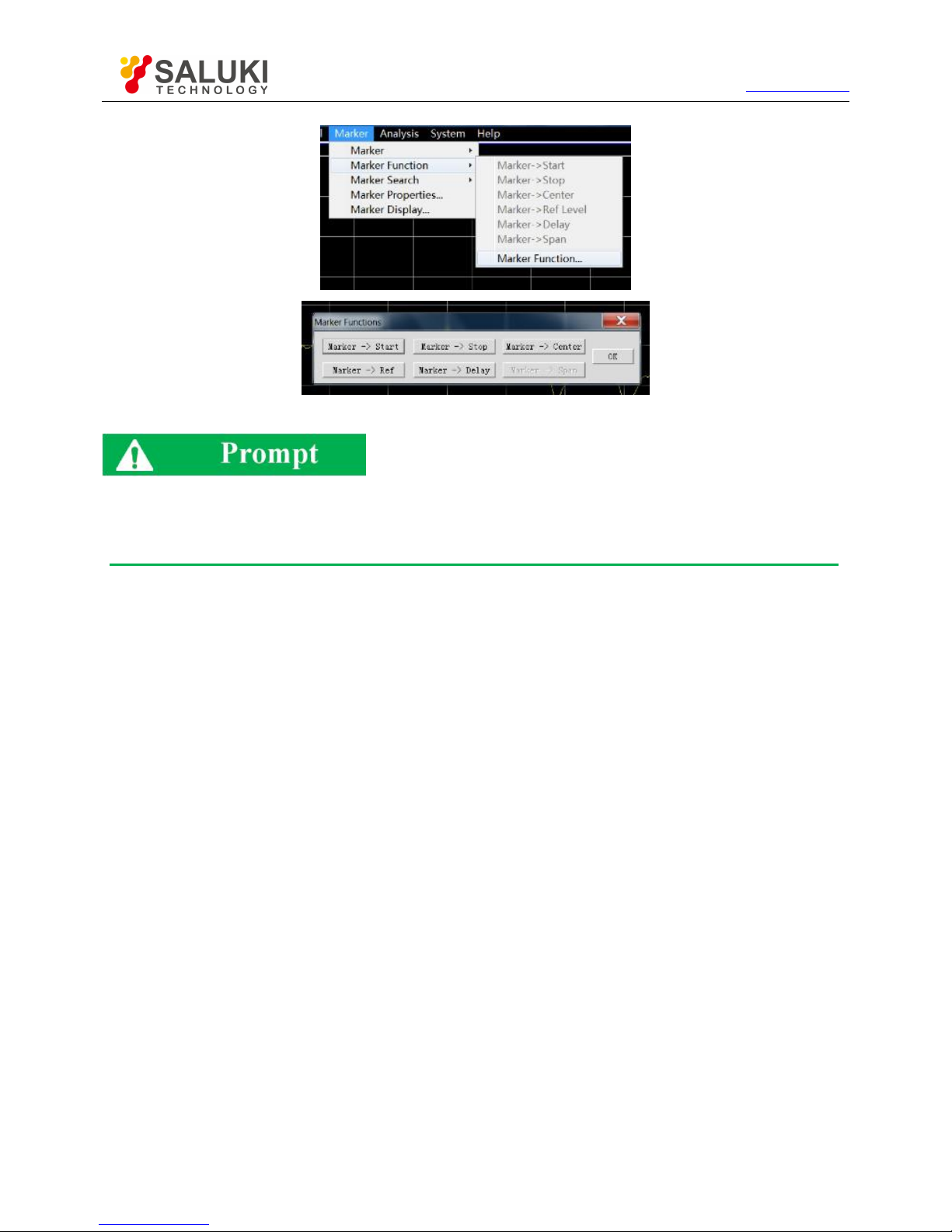
Tel: 886.2.2175 2930 Email: [email protected]
www.salukitec.com
50
Fig. 3.43 Measurement setups by marker Function Dialog Box
Soft key toolbar of marker function
The soft key toolbar of the marker function can be used to set the starting value, ending value, center value, reference value and
delay.
1) marker function dialog box
a) [Marker > Start] button
Click it to set the sweep start value to be equal to the stimulate value of the active marker.
b) [Marker > Stop] button
Click it to set the sweep end value to be equal to the stimulate value of the active marker.
c) [Marker > Center] button
Click it to set the sweep center value to be equal to the stimulate value of the active marker.
d) [Marker > Ref level] button
Click it to set the sweep reference value to be equal to the stimulate value of the active marker.
e) [Marker > Delay] button
Click it and the electrical delay of the reception path will be adjusted according to the phase slope of the active marker. In this case,
the phase trace near the active marker will be flattened. This function can be used to measure the electrical length and phase offset. It
is only applicable to ratio measurement.
f) [Marker > Span] button
Click it to set the sweep span value to be equal to the stimulate difference (△marker) between the active marker and reference
marker. This button is effective only when the △marker function of the active marker is enabled.
3.5.1.5.
Advanced marker option setting
1) Use of advanced marker option function
Menu path: [Marker] > [Marker] > [Marker...]. The marker dialog box will be displayed. Click the [Advanced marker...] button. The
advanced marker dialog box will appear.
2) Advanced marker option dialog box
Page 51

Tel: 886.2.2175 2930 Email: [email protected]
www.salukitec.com
51
a) [Marker] box
Select the marker to be set.
b) [Open] check box
If this check box is selected, the corresponding marker will be displayed on the screen. If this check box is cleared, the marker display
will be shut down.
c) [Discrete] check box
If this check box is selected, the data of the actual measurement point will be displayed. If this check box is cleared, the interpolation
data point between measurement points is still displayed.
d) [Format] box
Select the marker data format. The marker data format may be different from the format of trace data on the screen. The above
formats are identical in the default mode.
e) Marker type zone
[Normal] option box
The X-axis location of the standard marker is fixed, while the Y-axis location changes with the trace data amplitude. The marker can
be moved right and left on the X-axis by changing the stimulus value.
[Fixed] option box
The X-axis and Y-axis coordinates of the marker set to be of fixed type remain fixed on the trace and do not change with the trace data
amplitude. The marker can be moved on the X-axis by changing the stimulus value, however, the Y-axis coordinate remains
unchanged. This kind of marker is mainly used to observe changes of trace data. For example, the fix marker can be used to compare
insertion loss changes before and after filter tuning.
3.5.1.6. Marker list
1) Marker list
All marker data of the active data can be displayed by opening the marker list, in the format specified for the corresponding data. The
marker list will be opened and closed in the following method.
2) Open/Close method
Menu path 1: [Marker] > [Marker] > [Show Table] to open the marker list or [Hide Table] to close the marker list.
Page 52
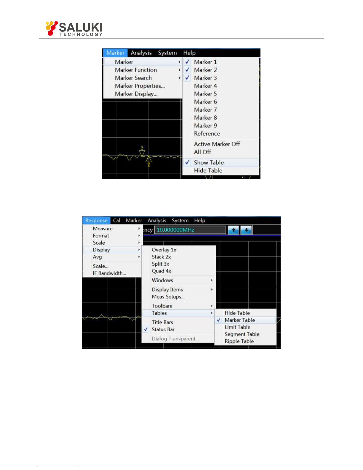
Tel: 886.2.2175 2930 Email: [email protected]
www.salukitec.com
52
Fig. 3.44 marker List Setting by marker Menu
Menu path 2: [Response] > [Display] > [List] > [Marker list].
If "√" is marked, the marker list will be opened; otherwise, the marker list will be closed.
Fig. 3.45 marker List Setting by "View" Menu
3.5.2.
Trace Operation and Statistics
The analyzer supports four kinds of mathematical operation of the current active trace and the trace in the memory. In addition, the
analyzer has three functions of trace statistics: average, offset and peak-peak value.
Trace operation
Trace statistics
3.5.2.1. Trace Operation
1) Setting the method of trace operation
Page 53
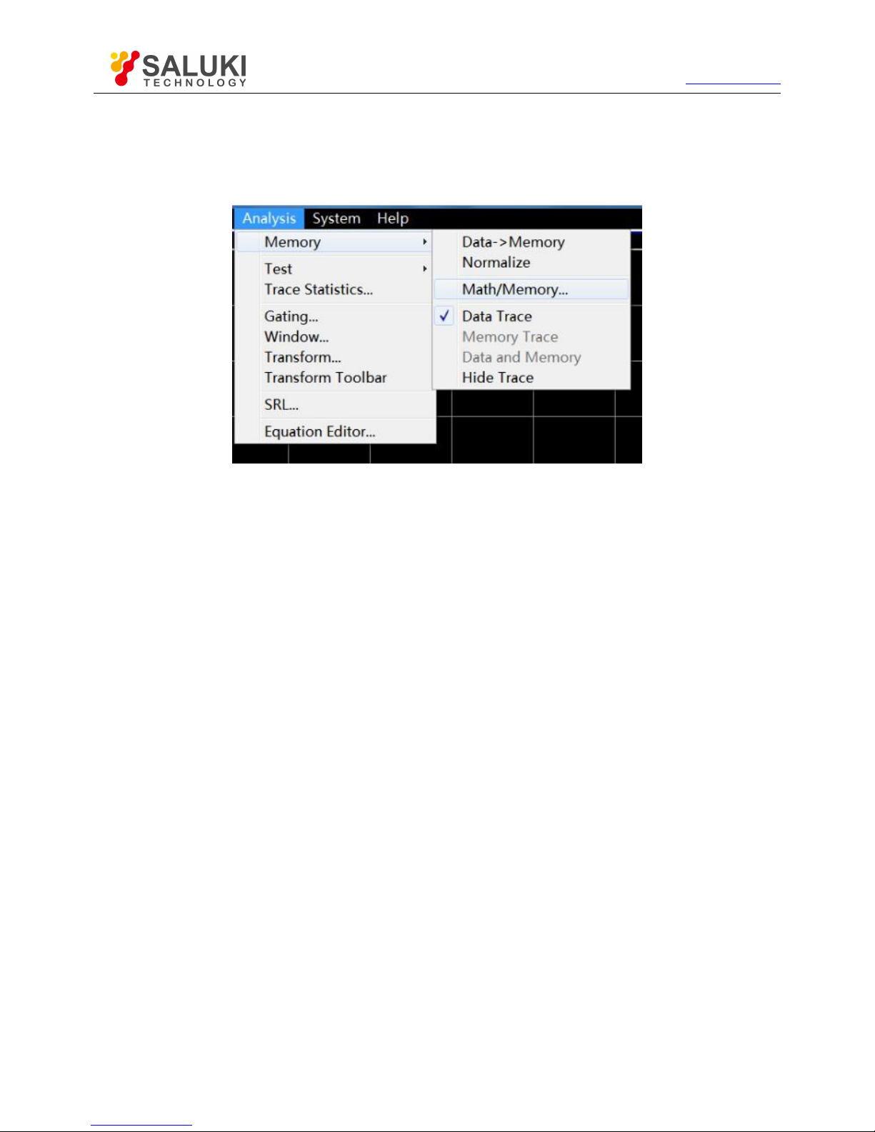
Tel: 886.2.2175 2930 Email: [email protected]
www.salukitec.com
53
One trace must be stored in the memory before setting the method of trace operation or performing any kind of trace operation. trace
operation is a kind of vector operation based on plural data before display formatting. It is set in the following method.
Menu path: [Analysis] > [Memory] > [Math/Memory...]. Then the operation/storage dialog box will appear.
Fig. 3.46 Setting of Trace Operation
2) Math/Memory dialog box
a) [Data > Memory] button
Save the current measurement data into the memory.
b) [Trace View Options] box
The [Trace View Options] box is used to select the type of trace operation. The analyzer supports the following operations.
Data
No mathematical operation.
Data+storage
The displayed trace data are the measured data plus stored trace data.
Data-storage
The displayed trace data are the measured data minus stored trace data. This function can be used for simple correction of errors. At
first, store the measured vector error into the memory, and then reduce the measurement data of the tested device by the measured
error.
. Data * storage
The displayed trace data are the measured data multiplied by the stored trace data.
Data/storage
The displayed trace data are the measured data divided by the stored trace data. This function is mainly used to measure the ratio,
such as the gain and attenuation.
c) Data display selection zone
[Data trace] option box
Only display the data trace.
[Memory trace] option box
Page 54
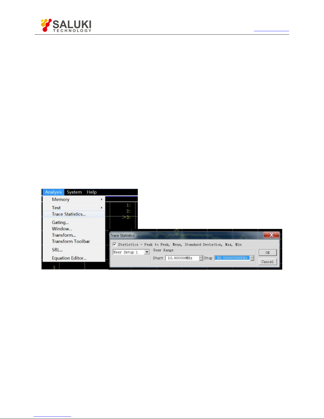
Tel: 886.2.2175 2930 Email: [email protected]
www.salukitec.com
54
Only display the memory trace.
[Data and memory] option box
Display the data trace and memory trace at the same time.
3.5.2.2.
Trace Statistics
The analyzer has three functions of trace statistics: mean, offset and peak-peak value. The statistical values can be calculated within
the whole stimulus bandwidth or user-defined bandwidth. Each channel supports nine user setting ranges, which are the same as the
search domains set by user in the function of marker search. The same memory address is applied, so the same stimulus settings are
shared. If the search domain to be set by the channel user is defined by marker search, the same stimulus settings can be called by
selecting the corresponding user settings in trace statistics. The ranges of user settings are allowed to be overlapping.
It is not required to search the maximum and minimum value in the function of trace statistics, and the peak-peak value of pass band
ripple can be measured easily. The statistical values of trace are calculated according to the data display format.
Rectangular coordinate format: the statistical values of trace are calculated according to the displayed scalar data.
Polar coordinate and Smith chart format: the statistical values of trace are calculated according to the value displayed in the log
magnitude format.
3) Activation of trace statistics
Menu path: [Analysis] > [Trace statistics]. The dialog box of trace statistics will appear.
Fig. 3.47 Dialog Box of trace Statistics
4) Dialog box of Trace statistics
a) [Statistics > Peak to Peak, Mean, Standard Deviation, Max, Min] check box
If this check box is selected, the function of trace statistics will be enabled. If this check box is cleared, the function of trace statistics
will be disabled.
b) [Span] box
Set the span of trace statistics. Nine user settings can be selected within the whole bandwidth or customized, or the user settings can
be customized through the marker search dialog box.
c) User domain definition zone
[Start] box
Customize the starting value of the user setting span.
[Stop] box
Customize the ending value of the user setting span.
Page 55
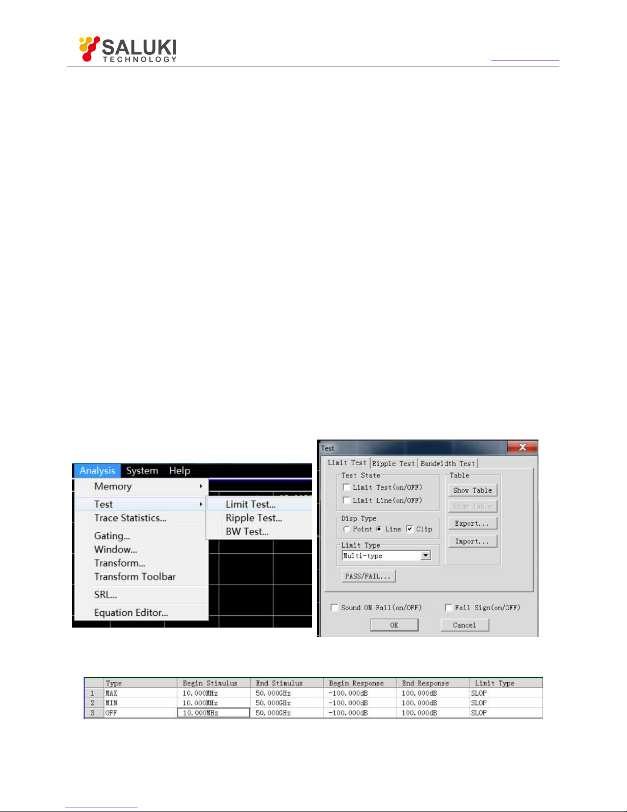
Tel: 886.2.2175 2930 Email: [email protected]
www.salukitec.com
55
3.5.3.
Limit Test
The limit test function is used to compare the measured data and defined constraints (limits). The limits defined by the user are
intuitively displayed on the screen in the limit line form. The limit lines have the following advantages:
Provide intuitive indicators for the device commissioning personnel.
Provide the standards of characteristic indicators of the device.
Provide the intuitive comparison between the measured data and indicators of the device.
The limit test function is used to compare the measured data and defined limits, and provide PASS and FAIL information. Each trace
supports up to 100 separate limit segments for accurate definition.
Create and edit limit line
Limit table
Set limit test
3.5.3.1. Creating and Editing of Limit Line
The analyzer supports creating of limit lines for all measured tracks. The limit line is composed of several separate segments which
are respectively determined by four coordinate values: X-axis starting and ending stimulate value and Y-axis starting and ending
response value. It is created and edited according to the limit table.
1) Menu path: [Analysis] > [Test] > [Limit test]. The test dialog box will appear.
2) Click [Show Table] in the dialog box to display the limit table.
3) Click [OK] to close the dialog box.
4) Click [Limit type] in the limit test dialog box and select the limit test type in the drop-down box.
Fig. 3.48 Limit Test
3.5.3.2. Limit Table
Fig. 3.49 Limit Table
“Type” Column
Page 56

Tel: 886.2.2175 2930 Email: [email protected]
www.salukitec.com
56
The Type box is used to set the limit test type:
MAX: the limit test fails if the trace is above the limit segment.
MIN: the limit test fails if the trace is below the limit segment.
OFF: disable the test of the limit segment.
“Begin Stimulus” / “End Stimulus” Column
Set the starting and ending stimulus value of the limit segment (i.e. X-axis starting and ending coordinate of the limit segment).
“Begin Response” Column and “Ending response” Column
Set the starting and ending response value of the limit segment (i.e. Y-axis starting and ending coordinate of the limit segment).
“Limit type” Column
Set the limit line display mode of the limit test:
SLOP: display the slope limit line.
FLAT: display the flat limit line.
POINT: display the point limit line.
3.5.3.3.
Setting of Limit Test
After creating the limit line, select the mode of displaying or hiding the limit line of one trace. Even if the limit line is hided, the
corresponding limit test is still effective. The limit test is not applicable to the stored trace. You can select to send the warning sound
and display the failure sign (FAIL) in case of the failure of limit test. When the limit test function is enabled, the trace of the failure part
is red in the default mode. You can change the limit failure color in the Color setting" of the right-click menu of the mouse, and the
trace color of the passing part remains unchanged.
1) Setting method
a) Menu path: [Analysis] > [Test] - [Limit test]. The test dialog box will appear.
b) Set the limit test in the dialog box.
c) Click [OK] to close the dialog box.
The limit test can only be done at the actual sweep measurement point. The instrument can still pass the limit test if only a few sweep
points are applied and the performance indicators of the tested device may not conform to the requirements. Therefore, sufficient
sweep points should be applied in actual measurement of the limit test.
2) Limit test dialog box
[Limit test ON/OFF] check box
If this check box is selected, the limit test of the active trace will be enabled. If this check box is cleared, the limit test of the active
trace will be disabled.
[Limit line display ON/OFF] check box
If this check box is selected, the limit line of the active trace will be displayed on the screen. If this check box is cleared, the limit line
display of the active trace will be turned off, however, the limit test function will not be affected.
[SOUND on Fail (ON/OFF)] check box
If this check box is selected, the buzzer will send the warning sound in case of failure of the trace data point test.
[FAIL Sign (ON/OFF)] check box
If this check box is selected, the FAIL sign will be displayed on the screen in case of failure of the trace data point test.
Page 57

Tel: 886.2.2175 2930 Email: [email protected]
www.salukitec.com
57
[Point] option box
If this box is selected, the discrete limit value corresponding to the measurement data point will be indicated with the symbol "v"
(measurement type: MAX) and "^" (measurement type: MIN).
[Line] option box
If this box is selected, all the discrete limit setting points will be connected through a line.
[Show table] button
Click it to display and edit the limit table. If the limit table is opened, this button will be disabled.
[Hide table] button
Click it to close the limit table display. If the limit table is closed, this button will be disabled.
[Export] button
Click it and the storage dialog box will pop up. You can select the storage path, and the file will be saved in the “*.csv” format.
[Import] button
Click it and the storage dialog box will pop up. Select the storage path of the file to be opened, and the file will be opened in the *.csv"
format.
[Limit type] drop-down option box
Click this drop-down option box to select the limit test type. Four types are provided in total: multi-type limit line, slope limit line,
single-point limit line and flat limit line.
3.5.4.
Ripple Test
The conformity of test results can be evaluated by setting the ripple limit of the ripple test. The measured data and defined ripple limit
are compared in the test. The PASS and FAIL information will be provided, and the measurement results will be intuitively displayed
on the screen. Each trace supports 12 separate limit segments at most. You can set the starting stimulus, ending stimulus and
maximum fluctuation of each limit segment. The stimulus settings of different segments may be overlapping.
3.5.4.1. Creating and Editing of Ripple Limit Line
The ripple limit test can be done to several tracks at the same time. The ripple limit can be set after the trace is activated.
1) Setting method
a) Menu path: [Analysis] > [Test] > [Ripple test]. The test dialog box will appear.
b) Click the [Show table] button in the dialog box to open the ripple limit table.
Page 58
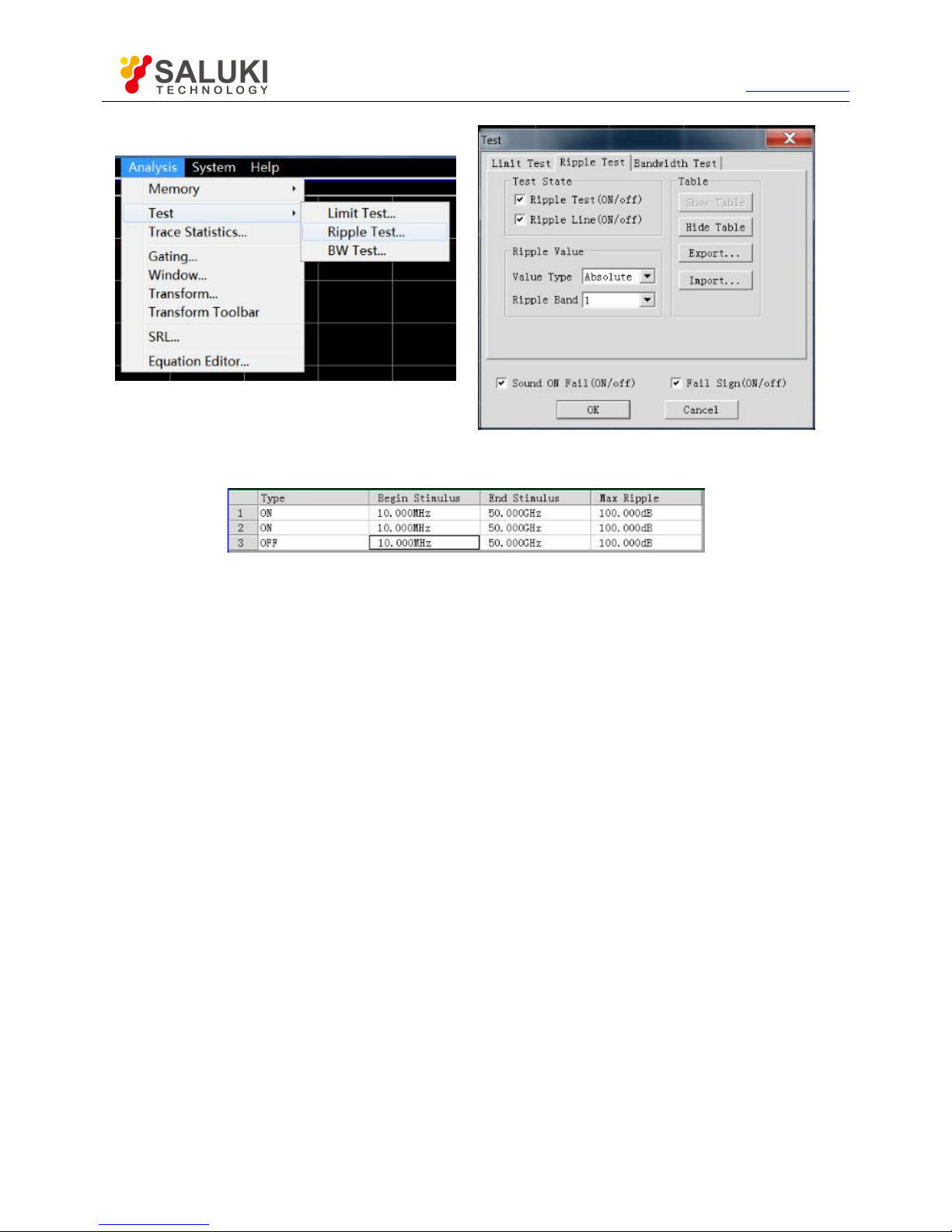
Tel: 886.2.2175 2930 Email: [email protected]
www.salukitec.com
58
Fig. 3.50 Ripple Test Dialog Box
2) Ripple limit table
Fig. 3.51 Ripple Limit Table
“Type” column
The "Type" column is used to set the limit test type:
ON: enable the test of the limit segment.
OFF: disable the test of the limit segment.
“Begin Stimulus” column
Set the starting and ending stimulus value of the ripple limit segment.
“End Stimulus” column
Set the maximum fluctuation of the test line of the ripple limit segment test.
3.5.4.2.
Setting of Ripple Test
After creating the ripple limit line, select the mode of displaying or hiding the ripple limit line of one trace. Even if the limit line is hided,
the corresponding ripple test is still effective. You can select to send the warning sound and display the failure sign (FAIL) in case of
the failure of ripple test. When the ripple test function is enabled, the trace of the failure part is red in the default mode. You can
change the limit failure color in the "Color setting" of the right-click menu of the mouse, and the trace color of the passing part remains
unchanged.
Menu path: [Analysis] > [Test] - [Ripple test]. The test dialog box will appear.
The ripple test can only be done at the actual sweep measurement point. The instrument can still pass the ripple test if only a few
sweep points are applied and the performance indicators of the tested device may not conform to the requirements. Therefore,
sufficient sweep points should be applied in actual measurement of the limit test.
Ripple test dialog box
[Ripple test on/OFF] check box
If this check box is selected, the ripple test of the active trace will be enabled. If this check box is cleared, the ripple test of the active
Page 59
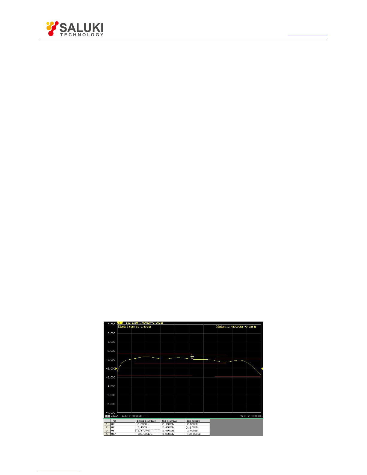
Tel: 886.2.2175 2930 Email: [email protected]
www.salukitec.com
59
trace will be disabled.
[Ripple line on/OFF] check box
If this check box is selected, the ripple line of the active trace will be displayed on the screen. If this check box is cleared, the ripple
line display of the active trace will be turned off, however, the ripple test function will not be affected.
[Sound ON Fail on/OFF] check box
If this check box is selected, the buzzer will send the warning sound in case of failure of the trace data point test.
[FAIL sign on/OFF] check box
If this check box is selected, the FAIL sign will be displayed on the screen in case of failure of the trace data point test.
[Show table] button
Click it to display and edit the ripple table. If the ripple table is opened, this button will be disabled.
[Hide table] button
Click it to close the ripple table display. If the ripple table is closed, this button will be disabled. [Export...] button
Click it and the storage dialog box will pop up. You can select the storage path, and the file will be saved in the "*.csv" format.
[Import...] button
Click it and the storage dialog box will pop up. Select the storage path of the file to be opened, and the file will be opened in the "*.csv"
format.
[value type] drop-down option box
Click this drop-down option box to select the limit test type: none, absolute value and allowance. The default value is the absolute
value after start-up of the instrument.
[Ripple Band] drop-down option box
Click the drop-down option box to select the number of ripple limit segments to be opened. At most 12 segments can be opened.
3.5.4.3.
Display of Ripple Test Results
If the measurement results of ripple test conform to the requirements, "PASS" will be displayed in the upper left corner of the screen;
otherwise, "FAIL" will be displayed. "PASS" and "FAIL" of each trace will be respectively displayed if several tracks are tested at the
same time. The stimulus ranges of different ripple limit segments are allowed to be overlapping, and various ripple limits can be set.
Fig. 3.52 Ripple Test Results
Page 60
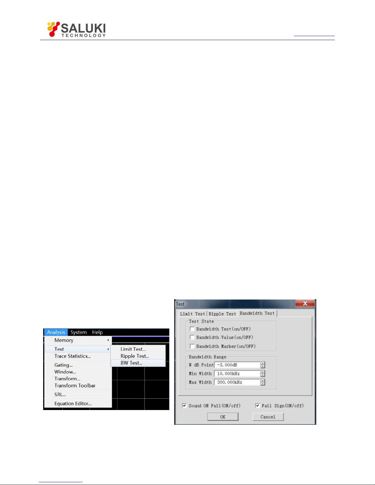
Tel: 886.2.2175 2930 Email: [email protected]
www.salukitec.com
60
3.5.5.
Bandwidth Test
The bandwidth test function is mainly used to test the bandwidth of the band pass filter.
The signal peak within the pass band can be found in the bandwidth test. Two points are respectively located at the specific amplitude
on both side of the pass band. The amplitude amplitude is lower than the signal peak and can be adjusted by setting the NdB point
(default setting: 3dB). The frequency range between the two points is the bandwidth of the tested filter.
The minimum bandwidth and maximum bandwidth allowed by the user can be set before the bandwidth test. The actual bandwidth will
be automatically compared with the above two values. In case of nonconformity, the FAIL information will be provided on the screen or
the sound will be utters, so that the user can intuitively check whether the properties of the tested device conforms to the
requirements.
3.5.5.1. Enabling and Setting of Bandwidth Test
Set the bandwidth threshold (NdB point), maximum bandwidth and minimum bandwidth before the bandwidth test. Several tracks can
be set.
1) Menu path: [Analysis] > [Test] > [BW test]. The test dialog box will appear.
2) Tick the [Bandwidth test on/OFF] check box in the dialog box to enable the bandwidth test.
3) Tick the [Bandwidth Value on/OFF] check box in the dialog box to display the tested bandwidth on the screen.
4) Tick the [Bandwidth Marker on/OFF] check box in the dialog box. The bandwidth location mark will be displayed on the screen.
5) Click the [NdB point] box to set the bandwidth threshold.
6) Click the [Min bandwidth] box to set the minimum bandwidth.
7) Click the [Max bandwidth] box to set the maximum bandwidth.
8) Tick the [Sound ON Fail on/OFF] check box in the dialog box. The sound prompt will be provided in case of failure of the
bandwidth test.
9) Tick the [FAIL sign on/OFF] check box in the dialog box. The FAIL prompt will be provided in case of failure of the bandwidth test.
10) Click [OK]. Thus the bandwidth test setting is completed.
Fig. 3.53 Dialog Box of Bandwidth Test
3.5.5.2. Display of Bandwidth Test Results
Bandwidth test results will be displayed in the upper left corner of the trace. If the test results are acceptable, "ASS" will be displayed.
Page 61
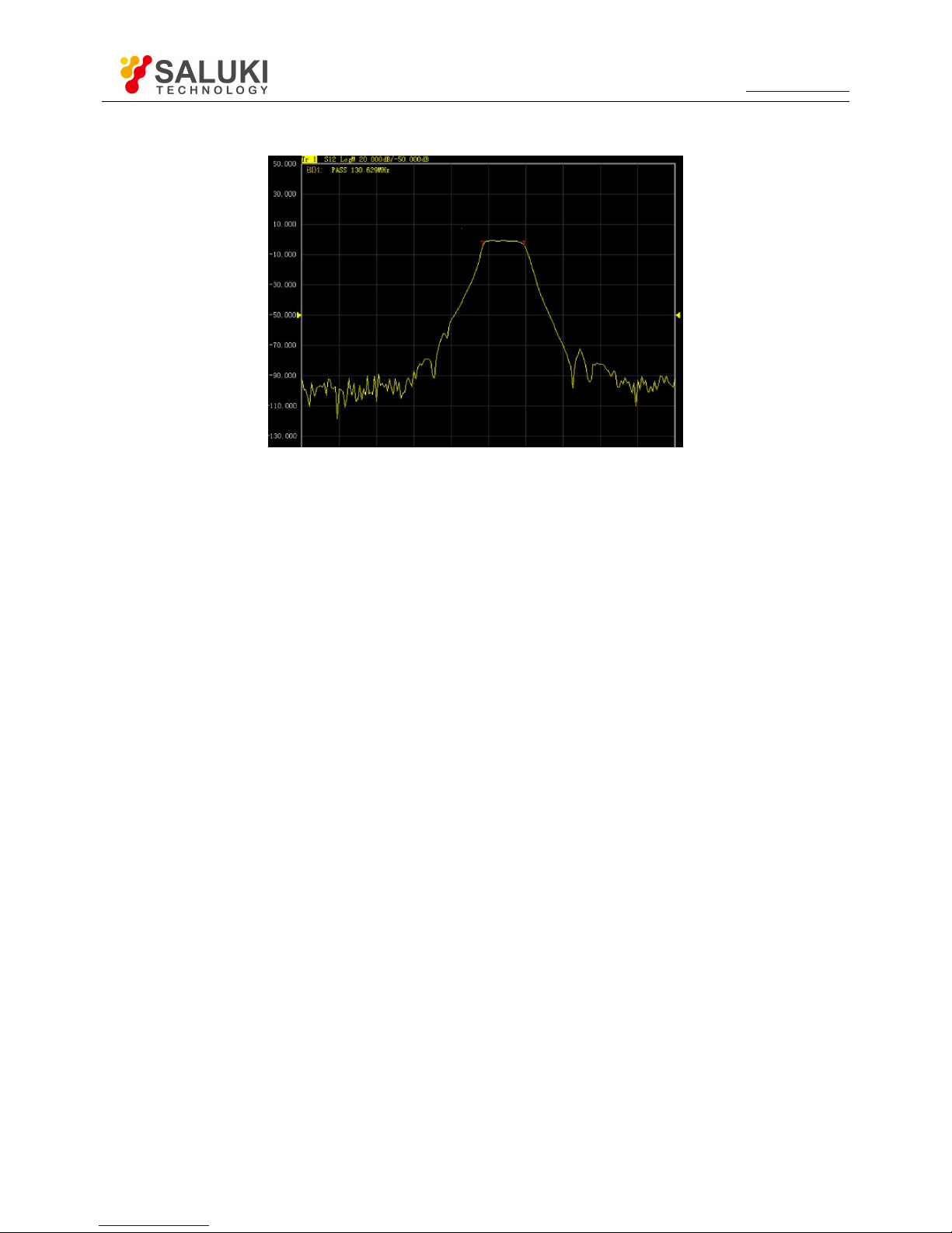
Tel: 886.2.2175 2930 Email: [email protected]
www.salukitec.com
61
The red T-type bandwidth marks will appear on both sides of the bandwidth.
Fig. 3.54 Display of Bandwidth Test Results
3.5.5.3.
Shutdown of Bandwidth Test
1) Click [Analysis] > [Test] > [BD test]. The test dialog box will appear.
2) Click the [Bandwidth test on/OFF] check box and remove the tick to shut down the bandwidth test.
3) Click the [Bandwidth value on/OFF] check box and remove the tick to shut down the test bandwidth value display.
4) Click the [Bandwidth mark on/OFF] check box and remove the tick to shut down the bandwidth position mark display.
5) Click [OK] to shut down the bandwidth test.
3.5.6. Equation Editor
Overview
Use of Equation Editor
Data and precautions of use of Equation Editor
Storage of Equation Editor data
3.5.6.1.
Overview
In order to facilitate illustration, the following two terms should be defined at first.
Reference trace: a trace used as data in the formula.
Formula trace: an active trace after formula calculation.
The user is allowed to enter an algebraic expression in the Equation Editor. The algebraic expression can be used for mathematical
operation of measurement data. Operation results can be displayed in the data trace form. Measurement data of the formula trace are
the data of one or more channel(s). The mathematical expression entered by the user is composed of the basic operator, built-in
function and parameters. Measurement parameters or trace data used in the formula are provided by the vector network analyzer. If a
calculation formula is entered into the formula input box and the activation box is ticked, the current active trace will become a formula
trace. The formula trace data are the data after operation, and the formula trace curve can be updated with data changes in a
real-time manner. Take the input formula S21/(1-S11) as an example. The value of each point on the formula trace is calculated by
S21/(1-S11) of the corresponding point. If the trace includes 201 points, the operation will be done 201 times by the expression, that is,
once for each point.
Measurement of a three-port device is not conventional for the analyzer, but can be done through the Equation Editor. If the user
Page 62
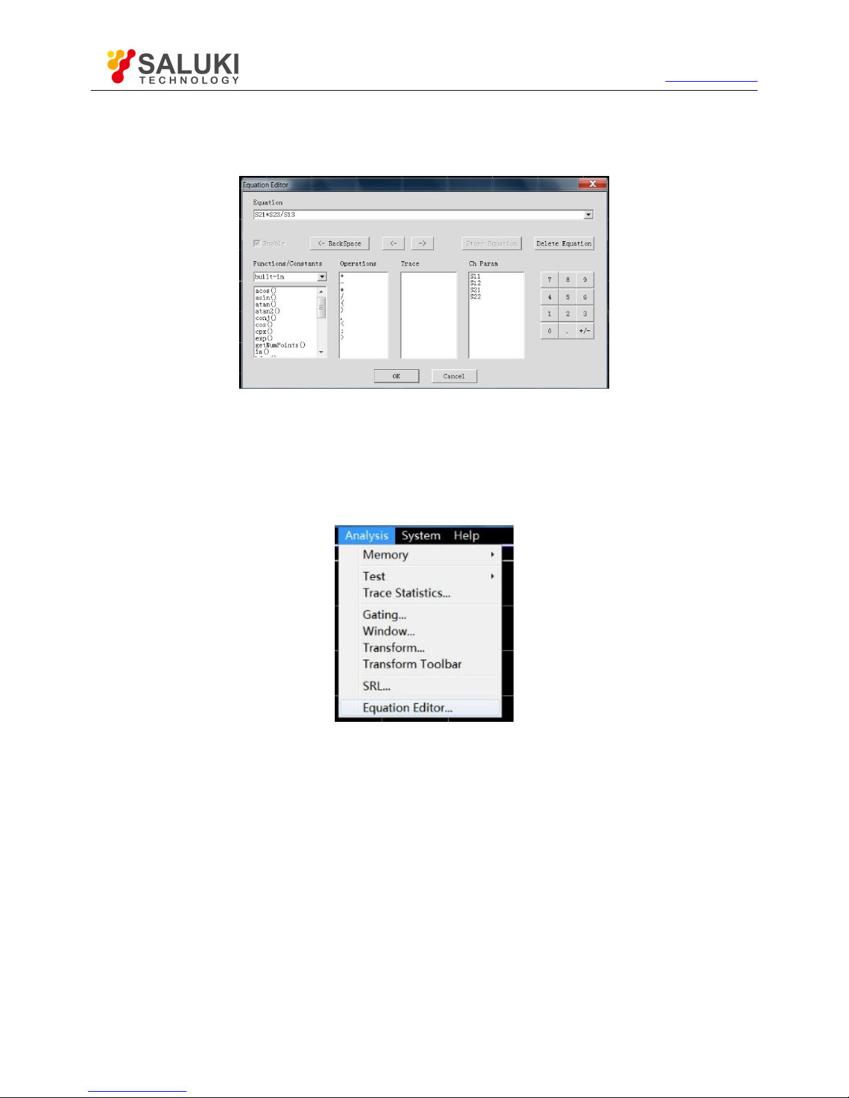
Tel: 886.2.2175 2930 Email: [email protected]
www.salukitec.com
62
expects to obtain a logarithmic formula trace, the following expression can be used: S21+S23- S13. However, the data used in the
Equation Editor are plural data with no format requirements. The user needs to enter the following formula: S21*S23/S13. After the
formula is entered, Eq=S12*S23/S13 will be displayed on the current active trace of the vector network analyzer.
Fig. 3.55 Dialog Box of Equation Editor
3.5.6.2. Use of Equation Editor
1) Open the Equation Editor dialog box.
Click the [Analysis] > [Equation Editor] in the menu of the vector network analyzer to open the Equation Editor dialog box, as shown in
Fig. 3.56.
Fig. 3.56 Equation Editor Menu
2) How to enter the formula in the Equation Editor dialog box
a) Function input
Click the function list under [Function and constants] in Fig. 3.55 and enter the function in the formula input box, or directly enter the
function through the keyboard.
b) Operator input
Click the operator list under [Operator] and enter the operator in the formula input box, or enter the operator through the keyboard.
c) Trace and channel input
Click the mouse to enter the trace and channel parameters among the options in the drop-down list of [Trace] or [Channel parameters],
as the formula parameters or variables, or enter the operator through the keyboard.
d) Data input
Enter the numbers through the number keys on the right side, or enter the operator through the keyboard.
Page 63
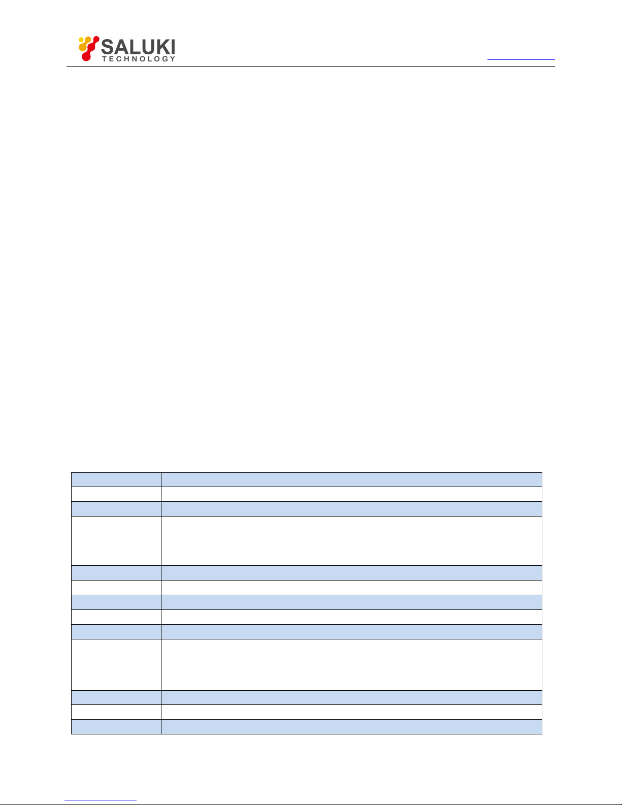
Tel: 886.2.2175 2930 Email: [email protected]
www.salukitec.com
63
3) “Activation” check box
The "activation" check box is ticked in the default mode. The formula entered by the user will be judged only when this check box is
ticked. If the formula is applicable to calculation, operation will be started. The expression Eq=XXX of the current formula will be
displayed on the active trace of the current active window of the vector network analyzer. If this check box is not ticked, operation will
not be started no matter whether the entered expression is applicable to calculation. In addition, if this check box is ticked but the
entered formula is not applicable to calculation (such as the case of "2+1+"), the check box will be gray.
4) Formula saving and deleting
Click [Save formula] to save any expression entered by the user in the formula input box, the formula will be saved in the drop-down
menu of the formula input box. Click the right drop-down arrow of the formula input box and select the formula in the drop-down list.
In addition, the user can click [Delete formula] to delete the formula in the formula input box.
5) Backspace button
[<-Backspace]: used to delete one character in front of the marker. If there is no character on the left side, the marker position will
remain unchanged.
6) Leftward and rightward movement of marker
[<-]: used to move the current marker left for one character but not to delete the left character. If there is no character on the left side,
the marker position will remain unchanged.
[->]: used to move the current marker right for one character but not to delete the right character. If there is no character on the right
side, the marker position will remain unchanged.
7) Selection of functions and variables
The built-in function library is set in the default mode, including the commonly used formulas and constants to be selected by clicking.
The functions/constants are shown in Table 3.10. If the parameter of one function is of plural type, the scalar can be used as the
parameter. The scalar is a plural, with 0 as the imaginary part.
Table 3.10 List of Functions/Constants
acos(scalar a)
Return to the ACOS value of the parameter a in radian. The parameter a is a scalar.
asin(scalar a)
Return to the ASIN value of the parameter a in radian. The parameter a is a scalar.
atan(scalar a)
Return to the Atan value of the parameter a in radian. The parameter a is a scalar.
atan2
Return to the phase of the plural a in radian. Two parameter types can be applied:
atan2 (complex a): return to the phase in radian. The parameter a is a scalar.
atan2 (scalar a and scalar b): return to the phase in radian. The parameter a and b are scalars.
conj(complex a)
Return to the conjugate complex of the plural a.
cos(complex a)
Calculate the cosine value of the plural a. The real part and imaginary part of a are in radian.
cpx(scalar a,scalar b)
Return to a plural (a+jb). The parameter a and b are scalars.
getNumPoints()
Return to the number of the current sweep points.
im(complex a)
Return to the imaginary part of the parameter a.
kfac(rComplex a,
rComplex b,
rComplex c,
Return value k = (1-|a|^2-|d|^2+|a*d-b*c|^2)/(2*|b*c|). The parameter a, b, c and d are plurals.
ln(complex a)
Return to the natural logarithm of the plural a.
log10(complex a)
Return to the logarithm of 10 corresponding to the plural a.
mag(complex a)
Return to the modulus of the plural a. The parameter a is a plural.
Page 64
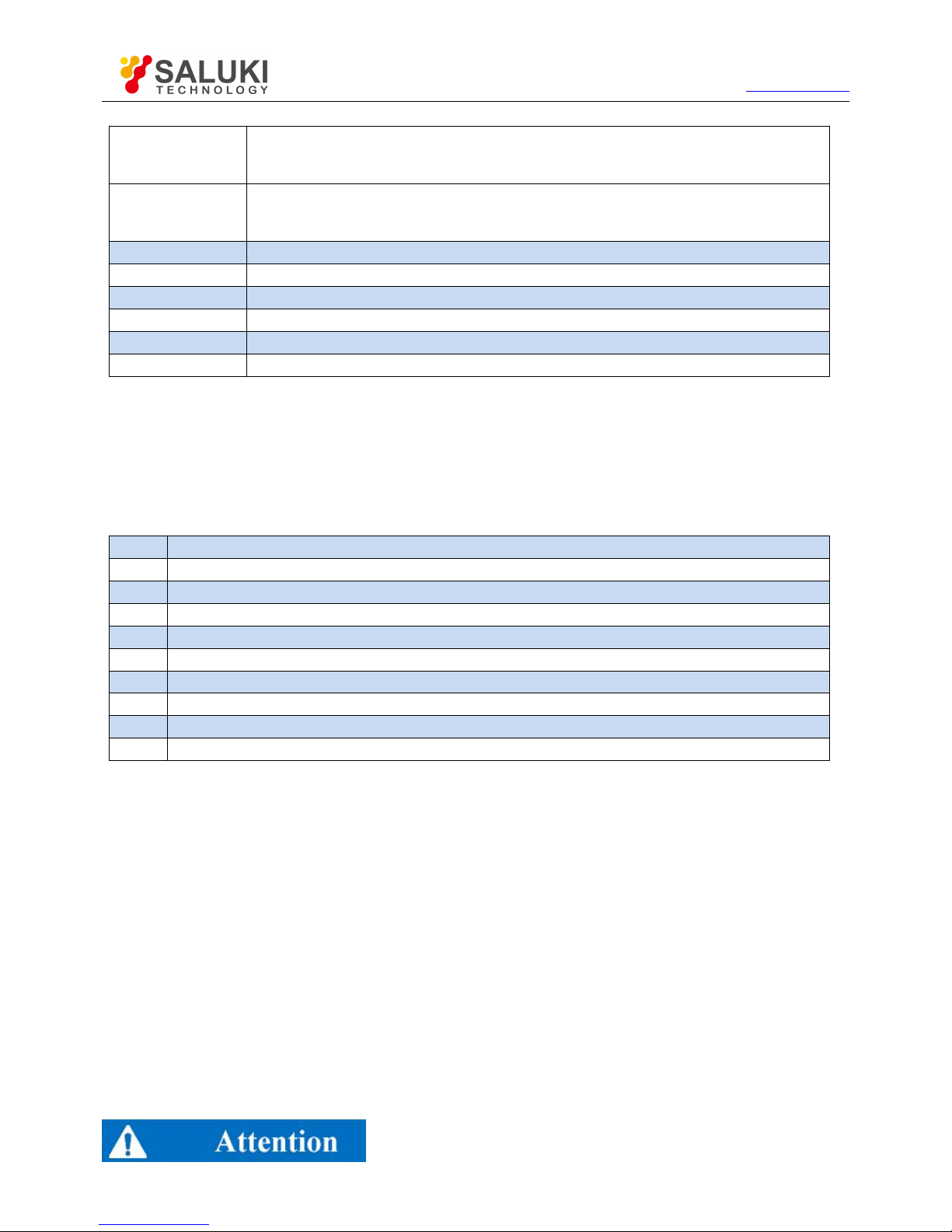
Tel: 886.2.2175 2930 Email: [email protected]
www.salukitec.com
64
mu1(complex a,complex b,
complex c,complex d)
Return value mu1 = (1-|a|^2)/(|d-conj(a)*(a*d-b*c)|+|b*c|). The parameter a, b, c and d are plurals.
mu2(complex a,complex b,
complex c,complex d)
Return value mu2 = (1-|d|^2)/(|a-conj(d)*(a*d-b*c)|+|b*c|). The parameter a, b, c and d are plurals.
phase(complex a)
Return to atan2 (a), i.e. calculation phase, in radian. The parameter is a plural.
PI
Constant Pi, 3.141592.
re(complex a)
Return to the real part of the plural a. The plural a is a plural.
sin(complex a)
Return to the sine value of the plural a. The parameter a is a plural, in radian.
sqrt(complex a)
Return to the square root of the modulus of the plural a. The parameter a is a plural.
tan(complex a)
Return to the tangent value of the plural a. The parameter a is a plural, in radian.
8) Operator selection
Operations are shown in Table 3.11. The user can click the mouse to select the required operator, such as four basic operators, i.e."+",
"-", "*" and "/", as well as the left bracket and right bracket. In addition, the Equation Editor also supports direct input of plural data for
operation. To enter the plural constant 2+j3, the user should enter <2:3> into the Equation Editor to indicate the plural constant 2+j3.
To enter the (2+j3)*S11, the user should enter the expression <2:3>*S11 for operation.
Table 3.11 List of Operators
+
Addition operator
-
Subtraction operator
*
Multiplication operator
/
Division operator
(
Left bracket
)
Right bracket
,
Comma, used to separate several parameters.
<
Start symbol to enter the plural.
:
Used to separate the real part and imaginary part of the plural.
>
Ending symbol to enter the plural.
9) Trace data
The user can select the trace or trace data in the list below, but the current active trace cannot be selected.
10) Channel parameter data
The user can only select the S-parameter of the current active channel as the parameter data of the entered expression.
11) Number key zone
The user can enter numbers by clicking number keys in the number key zone, the positive and negative symbol by clicking [+/-] and
the decimal point by clicking [•].
3.5.6.3.
Data and Precautions of Use of Equation Editor
The data of each point of the formula trace can be calculated according to the data of the corresponding point on the reference trace.
If the trace includes 201 points, the calculation will be done 201 times by the formula, i.e. Once for each data point. If the current trace
is Tr4 and the formula is Tr2+S11, Tr4 will be the formula trace. Tr1 and S11 are the reference tracks of the formula trace. In addition,
the current active trace Tr4 in the display window of the vector network analyzer will be displayed as Tr4Eq=Tr2+S11. As shown in Fig.
3.57.
Page 65
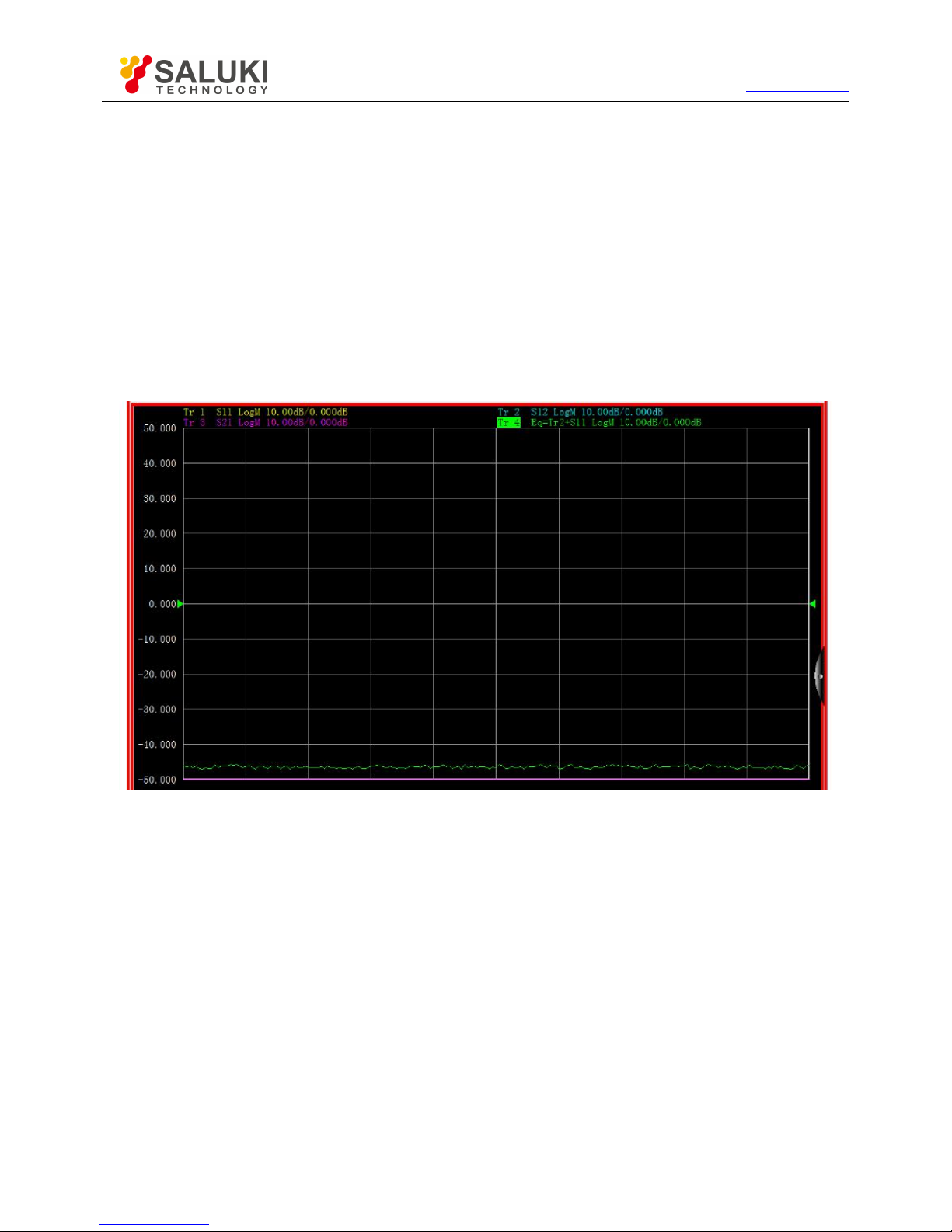
Tel: 886.2.2175 2930 Email: [email protected]
www.salukitec.com
65
Precautions for use of formula vector
1. If the formula is active and can be used for calculation, the original parameter will not be displayed on the current active trace.
Instead, the formula trace will be displayed. For example, if the current active trace is Tr4 S22 and the formula Tr2+S11 is
entered, the formula trace Tr4 Eq=Tr2+S11 will be displayed. However, if the entered formula cannot be used for calculation, the
original trace name will be displayed. For example, if "Tr2+S11+" is entered, the original Tr4 S22 will be displayed on the current
active trace.
2. The current active trace cannot be used as the reference trace of the formula trace. For example, the current active trace is Tr4,
Tr4 cannot be used as a parameter of the formula.
3. The reference trace can be selected from the S-parameter and memory tracks. Ensure that the memory track exists before using
it as a parameter; otherwise, the formula cannot be used for calculation.
4. The reference trace must be the displayed trace if the trace of another channel is used as the reference trace. The track must be
used in the Trx form. The numbers of data points of the reference trace and formula trace should be identical. For example, if the
number of data points of the reference trace is 201, the number of data points of the formula trace should also be 201.
Fig. 3.57 Formula Trace Display Window
3.5.6.4. Saving of Equation Editor Data
Formula data can be saved in the ".cti","*.prn" and "*.dat" format. However, the original names of measurement parameters are kept in
the saved file. For example, if the original name of Tr2 is S22 and the entered formula is 10+S22, the saved measurement parameter
name will remain unchanged, i.e. S22. The data will become the value of 10+S22. The equation trace cannot be saved as a data file in
the "*.snp" format.
3.6.Data output
Saving and calling of file
Printing of measurement data
3.6.1. Saving and Calling of File
S3602 series vector network analyzer supports the saving and calling of files in various formats.
3.6.1.1. Saving of File
Page 66
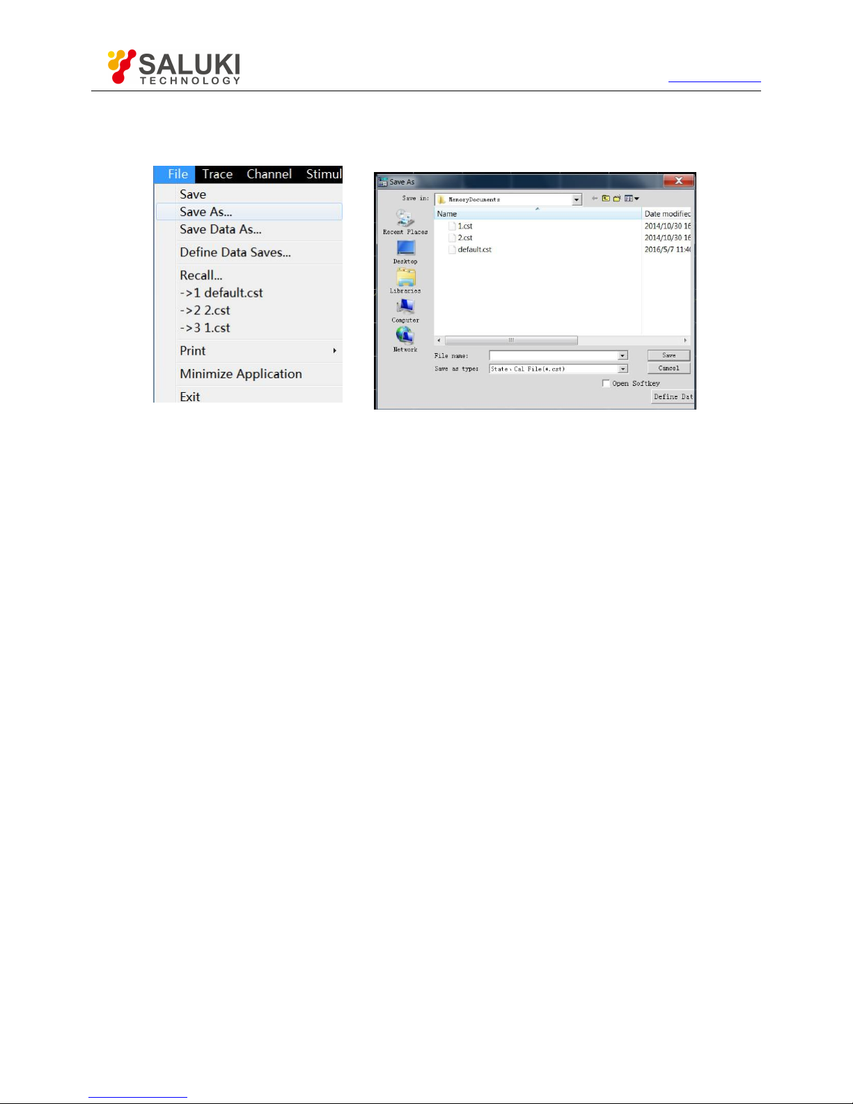
Tel: 886.2.2175 2930 Email: [email protected]
www.salukitec.com
66
1) Saving method
Menu path: [File] > [Save] > [Save]/[Save as...].
Fig. 3.58 Saving of File
2) File menu item: [Save]
Click [Save] to save the instrument status and calibration data int the default file (defaut.cst) of the specified directory. If the default file
exists, the dialog box to confirm whether to cover will appear.
3) File menu item: [Save as...]
Click [Save as...] to save the file in the dialog box.
a) [Save in] drop-down box
Display and set the saving path.
b) [File list] box
Display the holder under the current path and all files matching with the saving type. Click one file to set its name. Click the holder to
change the current path.
c) [File name] box
Display the entered file name or the file name clicked in the file list box.
d) [Saving as type] box
Select the saving type. The analyzer supports the following file types:
cst file
Save the instrument status and calibration data.
sta file
Only save the instrument status data.
cal file
Only save the instrument calibration data.
dat file
In this mode, the [Data save setting] dialog box will be opened, and the trace data file will be saved according to the user‘s
requirements.
Page 67
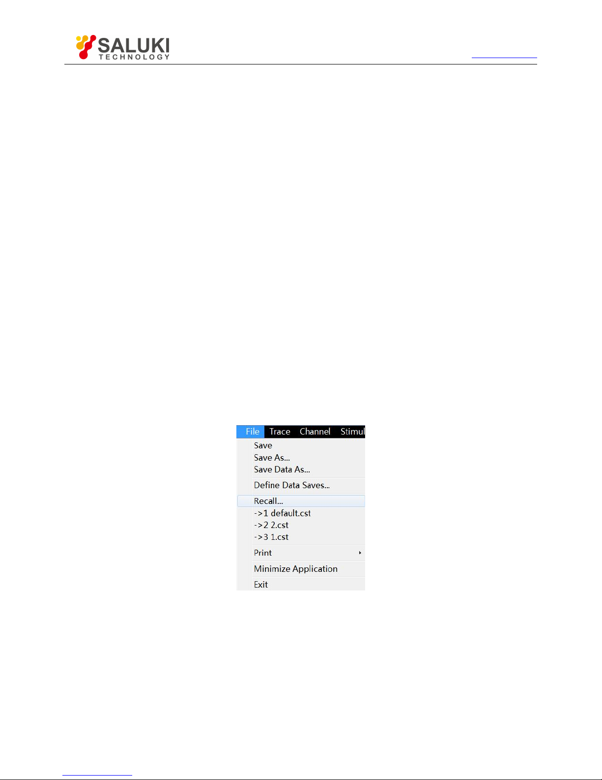
Tel: 886.2.2175 2930 Email: [email protected]
www.salukitec.com
67
Prn
Only save the current active trace data.
bmp file
Save the screen display information in the bitmap form.
3.6.1.2. Calling of File
1) Call status and calibration data:
a) sta file
The status data of the instrument are saved in the sta file, including the settings, trace data, limit line and marker.
b) cal file
Calibration data are saved in the cal file, excluding status data. The correction accuracy of calibration data is associated with the
status setting. To realize the highest accuracy of measurement, the instrument settings should be identical in file calling and calibration;
otherwise, the accuracy of calibration will not be guaranteed.
c) cst file
All measurement status and calibration data of the instrument are saved in the cst file, therefore, the cst file can be called to save
time.
2) File calling:
Menu path: [File] > [Call...]. The dialog box will appear.
Select the load file type in the [File type] box.
Set the call file directory through the [Search range] box and the [File list] below.
Fig. 3.59 File Calling
The file is called by the following methods:
Double-click the file to be called in the [File list] box.
Click the file to be called in the [File list] box and then click [Open].
Enter the name of the file to be called in the [File name] box and then click [Open].
3.6.1.3. Data File
Measurement results are saved in the ASCII format in data files. Data files can be edited with the text editing software and
spreadsheet software, but cannot be called by the analyzer. Three types of data files can be saved in the analyzer:
Page 68

Tel: 886.2.2175 2930 Email: [email protected]
www.salukitec.com
68
1) dat file
The "dat" file is used for saving measurement data of the active trace or all tracks in the formatted or unformatted form. Define the
data saving mode in the [Data save setting] dialog box.
The "at" file is saved by the following methods:
a) Menu path: [File] > [Save as...]. The [Save as...] dialog box will appear.
b) Set the file saving type as the data file (*.dat) in the [Saving type] box.
c) Set the saving directory in the [Save in] box and [File list] box.
d) Set the name of the file to be saved in the [File name] box.
e) Click [Save]. The [Data save setting] dialog box will appear.
f) Set the contents and format of the file to be saved. Click [Formatted data] or [Unformatted] to save the data file. Close the dialog
box.
[Save contents] zone
Define the trace data to be saved into the file.
a) [Default] radio box
Save the data of active tracks in all windows.
b) [One trace] radio box
Save the data of the current active trace.
c) [Window trace] radio box
Save the data of all tracks in the current active window.
d) [All tracks] radio box
Save the data of all tracks.
[Saving format] zone
a) [Auto] radio box
Save the trace data according to the actual display format.
b) [Log] radio box
Save the trace data in the logarithmic amplitude format.
c) [Linear format] radio box
Save the trace data in the linear amplitude format.
d) [Real part format] radio box
Save the trace data in the real part format.
e) [Imaginary part format] radio box
Save the trace data in the imaginary part format.
[Formatted data] button
Save the trace data in the format set in the [Saving format] zone.
[Unformatted] button
Page 69

Tel: 886.2.2175 2930 Email: [email protected]
www.salukitec.com
69
Save the trace data in the real/imaginary part format.
2) snp (s1p and s2p) file
The “snp" file is a kind of data output file. It can be called by the CAE (computer aided engineering) software (such as ADS of Agilent),
but cannot be called by the analyzer. The “s1p" file is used to save the characteristics of single-port devices, only including one S
parameter (S11 or S22). The "s2p" file is used to save the characteristics of 2-port devices, including four S parameters. If the full
2-port correction is started, four S parameters will be saved in the "s2p" file. If the full 2-port correction is shut down, measurement
data will be saved in the "s2p" file as much as possible. Example: if the full 2-port correction is shut down, the current active trace is
S11, but S21 is still measured in the channel, measurement results of S11 and S21 will be saved in the "s2p" file. As no effective
measurement data of S22 and S12 are provided, the corresponding data in the "s2p" file are 0.
The “snp" file is saved by the following method:
a) Menu path: [File] > [Save] > [Save as...]. The [Save as] dialog box will appear.
b) Set the saving type as the data file (*.s1p or *.s2p) in the [Saving type] box.
c) Set the saving directory in the [Save in] box and [File list] box.
d) Set the file name in the [File name] box.
e) Click [Save] to save data.
3) prn file
The prn file is used to save the measurement data of the active trace in lines and rows. Each line corresponds to one measurement
point. The first row corresponds to the stimulus value, while the second row corresponds to the response value. The format is as
follows:
S11
LogMag
LIN_SWEEP (Hz)
LOG_FORMAT (dB)
3.000000e+005
-9.232986e+000
7.502250e+008
-3.219671e-001
1.500150e+009
-6.892332e+000
2.250075e+009
-1.146303e+000
3.000000e+009
-1.245240e+001
The “prn" file is saved in the following method:
Menu path: [File] > [Save] > [Save as...]. The [Save as...] dialog box will appear.
Set the saving type as the list file (*.prn) in the [Saving type] box.
Set the saving directory in the [Save in] box and [File list] box.
Set the file name in the [File name] box. Click [Save] to save the file. Close the dialog box.
3.6.2. Printing of Measurement Contents
The analyzer supports the output of measurement contents through the printer or printing into the specified file. The local or
network printer can be used. The printer can be of parallel, serial or USB interface type. Add the printer in the WINDOWS
operating system.
3.6.2.1. Print Setup Method of print setting
Menu path: [File] > [Print] > [Page Setup]. Then the page setup dialog box will appear.
Page 70
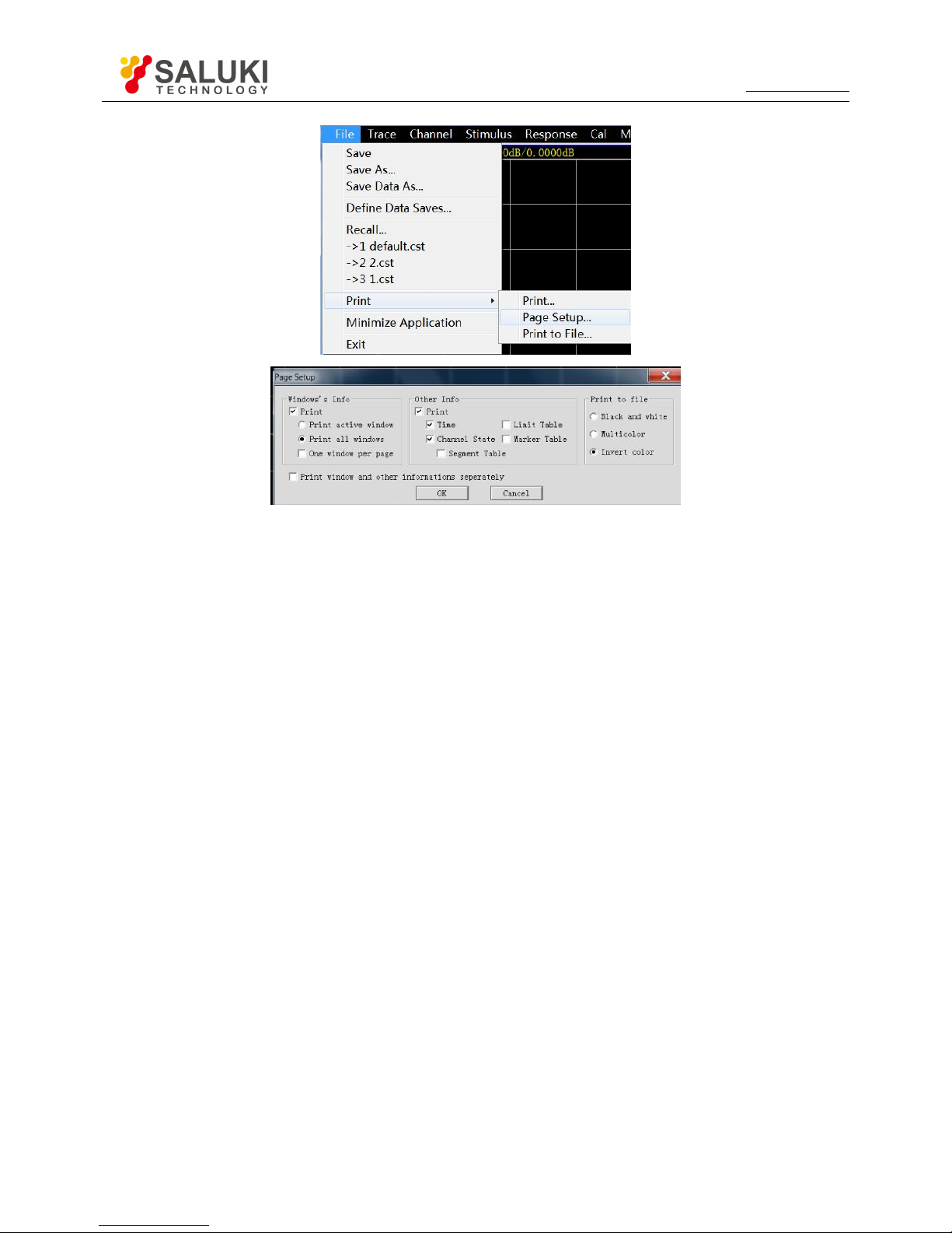
Tel: 886.2.2175 2930 Email: [email protected]
www.salukitec.com
70
Fig. 3.60 Print Setting
[Page Setup] dialog box
1) [Window info] zone
a) [Print] check box
If this check box is selected, the window trace information will be printed. If this check box is cleared, the window trace information will
not be printed. The following two check boxes are effectively only when the above check box is selected.
b) [One window per page] check box
If this check box is selected, only the information of one window will be printed. If this check box is cleared, the information of all
windows will be printed continuously, with no page breaks.
c) [Print active window] radio box
If this box is selected, only the information of the current active window will be printed.
d) [Print all windows] radio box
If this box is selected, only the information of the current active window will be printed.
2) [Other info] zone
a) [Print] check box
If this check box is selected, the channel setting information will be printed. The following check boxes are effectively only when this
check box is selected.
b) [Segment table], [Limit table], [marker table], [Channel statue] and [Time] check box
Select to print the corresponding information.
3) [Separately print window and other information] check box
If this check box is selected, the window and other information will be printed separately. If this check box is cleared, the above
information will be printed together.
3.6.2.2. Printing
Page 71
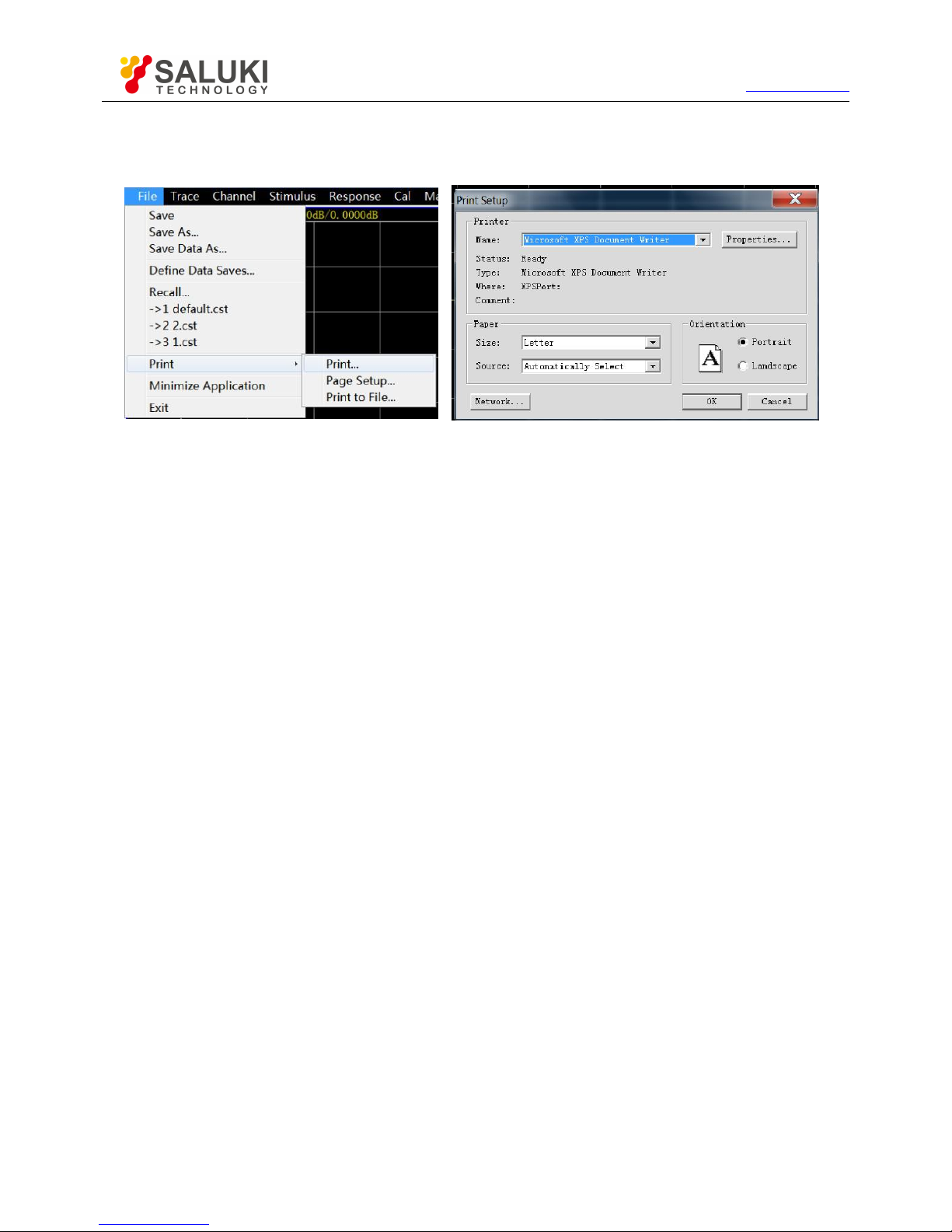
Tel: 886.2.2175 2930 Email: [email protected]
www.salukitec.com
71
After the printer is added and the print contents are set, measurement information can be output through the printer, as shown below:
Menu path: [File] > [Print] > [Print...]. The print setting dialog box will appear.
Fig. 3.61 Printing of Measurement Information
3.6.2.3.
Printing into File
The analyzer supports the output of print contents into the bitmap (bmp) file. To print several pages, various BMP files will be created
automatically, respectively corresponding to each page. The other files are identified in the file name (number).bmp" format, such as
amp.bmp, amp(1).bmp and amp(2).bmp. The printing method is as follows:
Menu path: [File] > [Print] > [Print to file...].
Set the file directory and name in the dialog box.
Click [Save] to save the file.
Page 72

Tel: 886.2.2175 2930 Email: [email protected]
www.salukitec.com
72
4. Measurement setups
This chapter mainly describes the operation of S3602 series network analyzers in measurement, creation of the measurement of
the known status by analyzer resetting, selection of Measurement setups, adjustment of the analyzer display so as to better
observe measurement results, specifically including:
Resetting of analyzer
Selection of measurement parameter
Setting of frequency range
Setting of signal power level
Setting of sweep
Trigger mode
Setting of data format and scale
Observation of multiple tracks and opening of multiple channels
Setting of analyzer display
4.1.
Resetting of Analyzer
Default reset state
User reset state
Resetting of analyzer
4.1.1. Default Reset State
Press the [Reset] on the front panel to return to the known default state, i.e. reset state. The reset state is set as follows:
1) Measurement parameter: S11
2) Frequency setting:
a) Starting frequency: 10MHz
b) Ending frequency: 13.5GHz/26.5GHz/43.5GHz/50GHz/67GHz
c) CW frequency: 2GHz
3) Power setting:
a) Test port power: -5dBm
b) Coupling port power: open
c) Attenuation: automatic
d) Attenuation values: 0dB
e) Power slope: closed
f) Slope: 0dB/GHz
4) Sweep setting:
a) sweep type: linear frequency
b) sweep time: automatic
Page 73
Tel: 886.2.2175 2930 Email: [email protected]
www.salukitec.com
73
c) Number of sweep points: 201
5) Segment sweep setting:
a) Number of open segments: 1
b) Starting frequency: 10MHz
c) Ending frequency: 13.5GHz/26.5GHz/43.5GHz/50GHz/67GHz
d) Number of points: 21
e) Power: -5dBm
f) Intermediate frequency bandwidth: 1kHz
6) Trigger setting:
a) Trigger source: internal
b) Trigger type: continuous scanning
7) Display format:
Format: logarithmic amplitude
The details of various formats are shown in Table 4.1.
Table 4.1 Default Format Setting of S3602 Series Vector Network Analyzers
Format
Scale
Reference position
Reference value
Logarithmic amplitude
≤10 dB50dB
phase
45o5
0
o
Group delay
10ns510fs
Linear amplitude
100mU
5
500mU
Standing wave ratio
1U56U
Real part2U5
0U
Imaginary part
2U50U
Polar coordinate
1U
None
1U
Smith chart
1U
None
1U
8) Response setting:
a) Number of channels: 1
b) Intermediate frequency bandwidth: 1kHz
c) Average: closed
d) Average factor: 1
e) Smoothing: closed
f) Smoothing factor: 2.49% of the value range
g) Electrical delay: 0s
h) Speed factor: 1
Page 74

Tel: 886.2.2175 2930 Email: [email protected]
www.salukitec.com
74
i) Phase shift: 0°
j) Trace display: data
9) Calibration setting:
a) Correction: closed
b) Interpolation: open
c) Calibration type: none
d) Calibration kit number: current calibration kit number
e) System impedance: 50Ω
f) Port extension: closed
g) Port extension value: 0s
10) Marker setting:
a) Initial frequency: full range of center frequency
b) Reference marker R: closed
c) Discrete marker: closed
d) Format: trace format
e) Type: standard
f) Marker search type: minimum
g) Search domain: full bandwidth
h) Marker table: empty
11) Limit test setting:
a) Limit test: closed
b) Limit line display: closed
c) FAIL sound warning: closed
12) Limit table setting:
a) Type: OFF
b) Initial stimulus: 10MHZ
c) Ending stimulus: 13.5GHz/26.5GHz/43.5GHz/50GHz/67GHz
d) Initial response: -100dB
e) Ending response: 100dB
13) Time domain transformation setting (optional):
a) Time domain transformation: closed
b) Transformation mode: bandpass
c) Transformation start: -5ns
d) Transformation end: 5ns
e) Kaiser window β factor: 6.0
Page 75
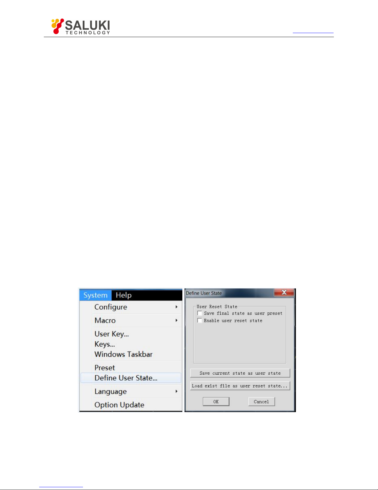
Tel: 886.2.2175 2930 Email: [email protected]
www.salukitec.com
75
f) Gate state: closed
g) Gate starting value: -5ns
h) Gate ending value: 5ns
i) Gate shape: standard
j) Gate type: bandpass
14) Full display setting:
a) Trace state: open
b) Frequency/stimulus: open
c) marker reading: open
d) Status bar: closed
4.1.2. User Reset State
The analyzer can be reset into the known default status or user-defined status. In the default mode, the analyzer is reset into the
default status. It can be reset into the user-defined status by means of setting. Specific steps of setting the user reset status are as
follows.
1) Menu path: [System] > [Define user state...]. Then the [Define user state...] dialog box will appear.
2) Click [Enable user reset status] and tick the check box.
Notes:
a) If you tick [Save final status as user preset], the final status before exiting the program will be saved as the user reset state.
b) Click [Save current status as user status]. Then the current settings of the analyzer will be saved as the user reset status.
c) To use the known status, click [Load exist file as user reset status]. Select the status in the dialog box, and open the file. Then
the selected file will be used as the user reset status file of the analyzer.
Fig. 4.1 Definition of User Reset Status
4.1.3. Resetting of Analyzer
Menu path: [System] > [Reset]
If the user reset state has been set, click [User reset].
Page 76
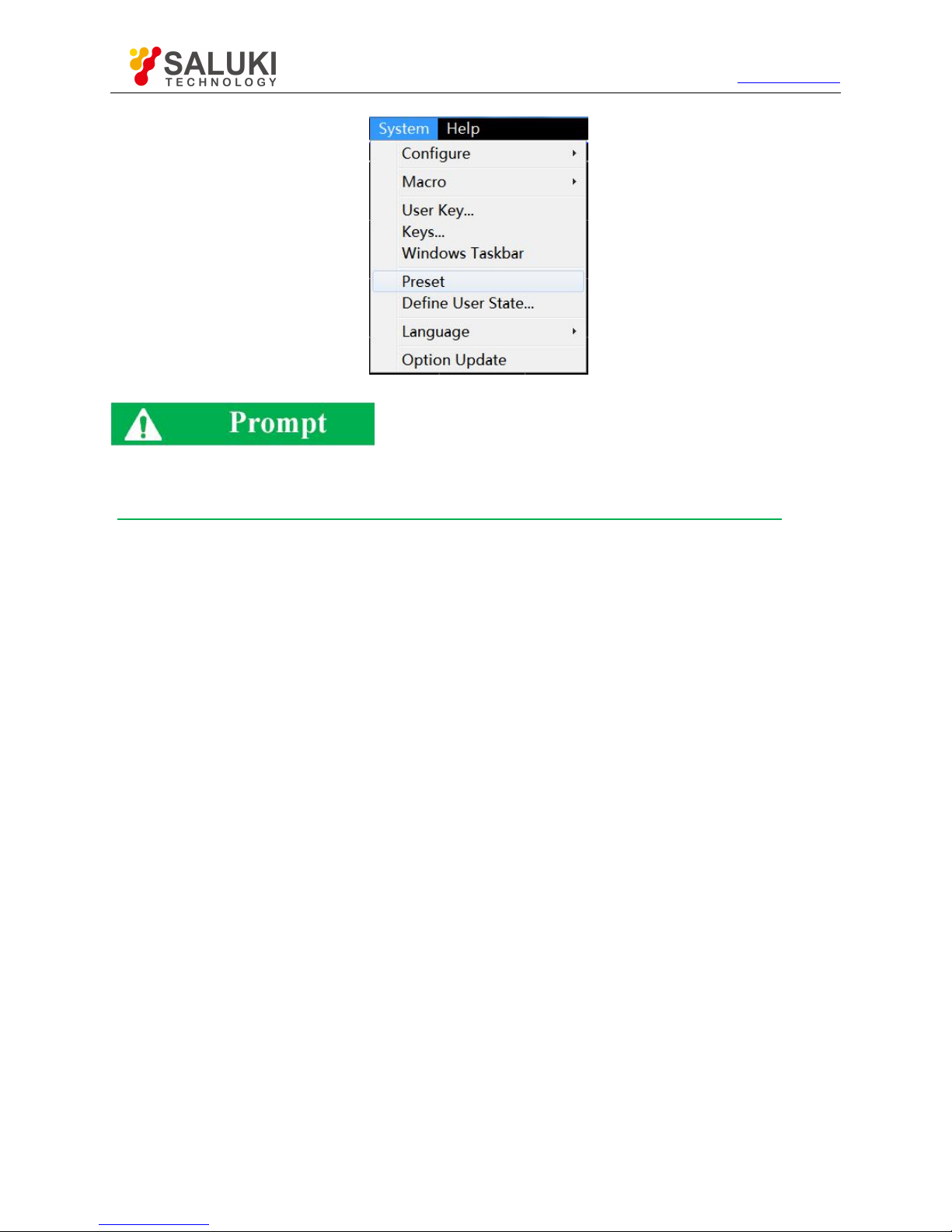
Tel: 886.2.2175 2930 Email: [email protected]
www.salukitec.com
76
Fig. 4.2 Resetting of Analyzer
[Reset] shortcut key
The [Reset] shortcut key is set in the functional key zone and shortcut menu bar.
4.2.
Selection of Measurement Parameter
The following parameters can be set in an S3602 series vector network analyzer to measure the electrical characteristics of
devices.
S parameter (fixed ratio)
Any ratio (custom ratio for measurement)
Non-ratio power measurement (absolute power measurement)
S parameter
Any ratio
Non-ratio power measurement
Change of trace measurement type
4.2.1.
Parameter S
1) Overview of Parameter S
The parameter S (scattering parameter) is used to describe the change of input signal and the reflection and transmission
characteristics of the tested device. The S-parameter is shown in the prescribed digit row, and indicates the proportion of two
complex vectors, i.e. S
output/input
, including the amplitude and phase information. The output refers to the output signal port number
of the tested device, and the input refers to the input signal port number of the tested device. The analyzer is equipped with four
test ports to test single-port, double-port, three-port and four-port devices.
For example, when one 2-port device is connected to Port 1 and 2, four parameters (S) can be measured at the same time.
In this case, the four parameters (S) of the 2-port device are respectively S11, S12, S21 and S22. Fig. 4.3 further shows the
parameter S, where:
a refers to the stimulus signal from the input to tested device.
b refers to the reflection and transmission signal (response signal) of the tested device.
The parameter S is a plural linear value. The measurement accuracy depends on the indicators of the calibrator and the adopted
Page 77
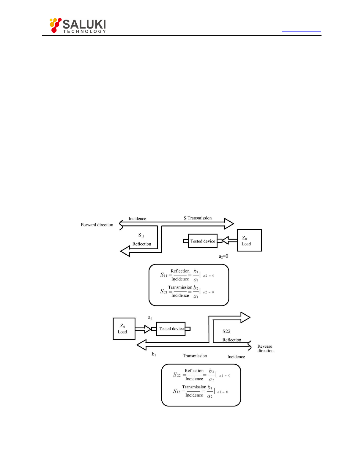
Tel: 886.2.2175 2930 Email: [email protected]
www.salukitec.com
77
technology of measurement connection, and is also associated with the connection of the non- measurement port (non-excited
port).
2) Application of parameter S
The following parameters can be measured with S.
a) Reflection measurement: SXX (X=1, 2, 3, 4)
1. Return loss
2. Standing wave ratio (SWR)
3. reflection coefficient
4. Impedance
5. S11, S22, S33 and S44
b) Transmission measurement: SXY (X=1, 2, 3, 4; Y=1, 2, 3, 4; X≠Y)
1. Insertion loss
2. Transmission coefficient
3. Group delay
4. SXY
The measurement of the 2-port device with Port 1 and 2 is taken as an example below to introduce the parameter S.
Fig. 4.3 Definition of Parameter S
3) New S measurement trace
Menu path: [Trace] > [New trace]. Click the S-parameter in the dialog box.
Page 78
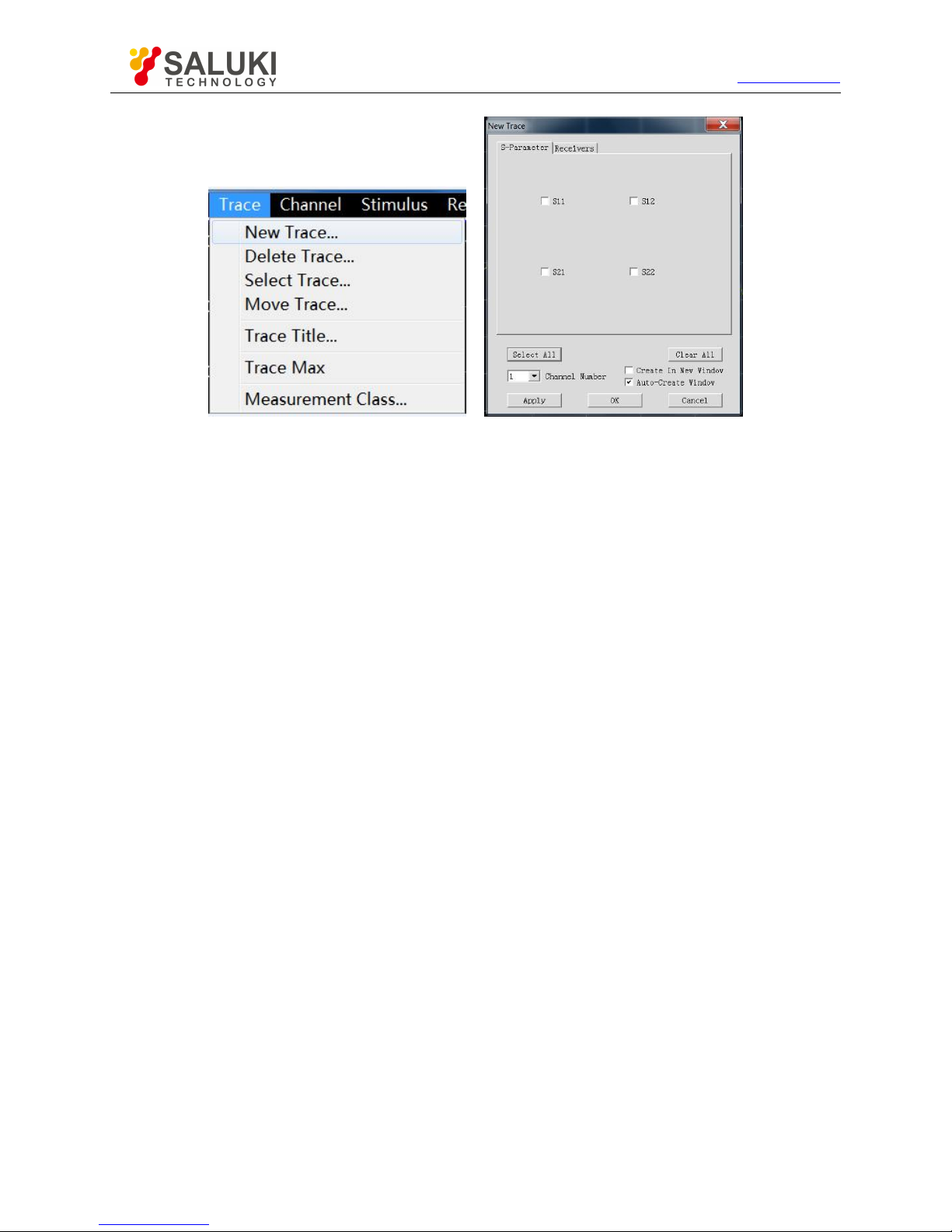
Tel: 886.2.2175 2930 Email: [email protected]
www.salukitec.com
78
Fig. 4.4 Definition of Parameter S
4) [New trace] dialog box
a) [S-Parameter] zone
Select the S parameter measurement trace to be created.
b) [Receiver] button
Open the dialog box to create any ratio or non-ratio power measurement trace.
c) [Balance parameter] button
Open the dialog box to create the balance parameter measurement trace.
d) [Channel selection] box
Select the channel where the new trace is located.
e) [Create in new window] check box
If this check box is selected, a trace will be created in the new window. If this check box is cleared, a trace will be created in the
current active window.
4.2.2. Any Ratio
The input signal and reference signal are selected from the receiver A, B, C, D, R1, R2, R3 or R4 for ratio measurement.
1) Create measurement trace of any ratio
Menu path: [Trace] > [New trace]. Click “Receiver" in the dialog box.
Page 79
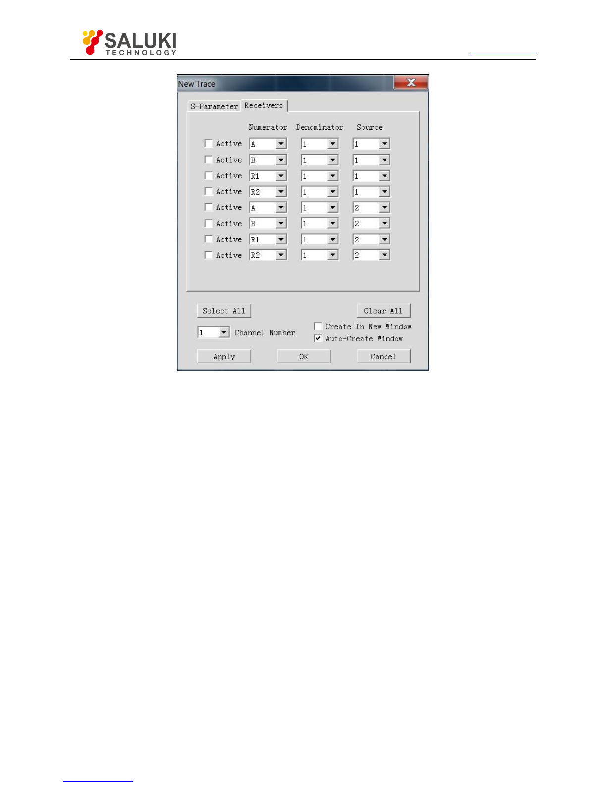
Tel: 886.2.2175 2930 Email: [email protected]
www.salukitec.com
79
Fig. 4.5 Definition of Parameter S
4.2.3.
Non-ratio Power Measurement
The absolute power of the receiver A, B, C, D, R1, R2, R3 and R4 can be measured in the non-ratio power measurement mode,
however, the phase, group delay and other items under the “average" function cannot be measured.
1) New non-ratio power measurement trace
Menu path: [Trace] > [New trace]. Click “Receiver" in the dialog box.
2) [New trace] dialog box (any ratio and non-ratio power measurement)
a) [Active] check box
Tick it to create a new trace.
b) [Numerator] zone
Select the numerator of any ratio measurement or the receiver for non-ratio power measurement.
c) [Denominator] zone
Select the denominator of any ratio measurement. The value is 1 in non-ratio power measurement.
d) [Source] box
Select the source signal output port of the analyzer.
e) [Channel Number] box
Select the channel for the new trace.
f) [Create in new window] check box
If this check box is selected, a trace will be created in the new window. If this check box is cleared, a trace will be created in the
current active window.
Page 80
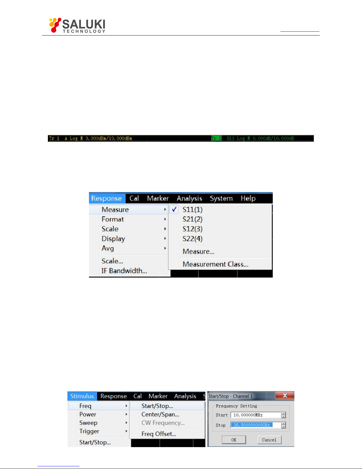
Tel: 886.2.2175 2930 Email: [email protected]
www.salukitec.com
80
g) [Automatically create window] check box
If this check box is ticked and the number of tracks in the window exceeds 8, excessive tracks will be automatically created in a
new window.
If this check box is cleared and the number of tracks in the window exceeds 8, excessive tracks will not be created.
4.2.4. Measurement mode of trace change
The trace must be activated before setting and modification.
1) Change the trace activation status
Click the [Trace status] button in the window. The corresponding trace will be activated.
Fig. 4.6 Change of trace Activation Status
2) Change the measurement parameter of the activated trace
Menu path: [Response] > [Measure].
The measure sub-menu will appear. Or, right-click the trace title bar, and click [Measure] in the menu, as shown in Fig. 4.7.
Fig. 4.7 Setting of Parameter S Measurement Mode of Activated Trace
4.3.Setting of Frequency Range
Frequency range: 10MHz-13.5GHz/26.5GHz/43.5GHz/50GHz/67GHz
Frequency resolution: 1Hz
1) Two ways of frequency range setting
a) Specify the start/stop frequency.
b) Specify the center frequency and frequency span.
2) Setting of start and Stop frequency
Menu path: [Stimulus] > [Frequency]
Page 81
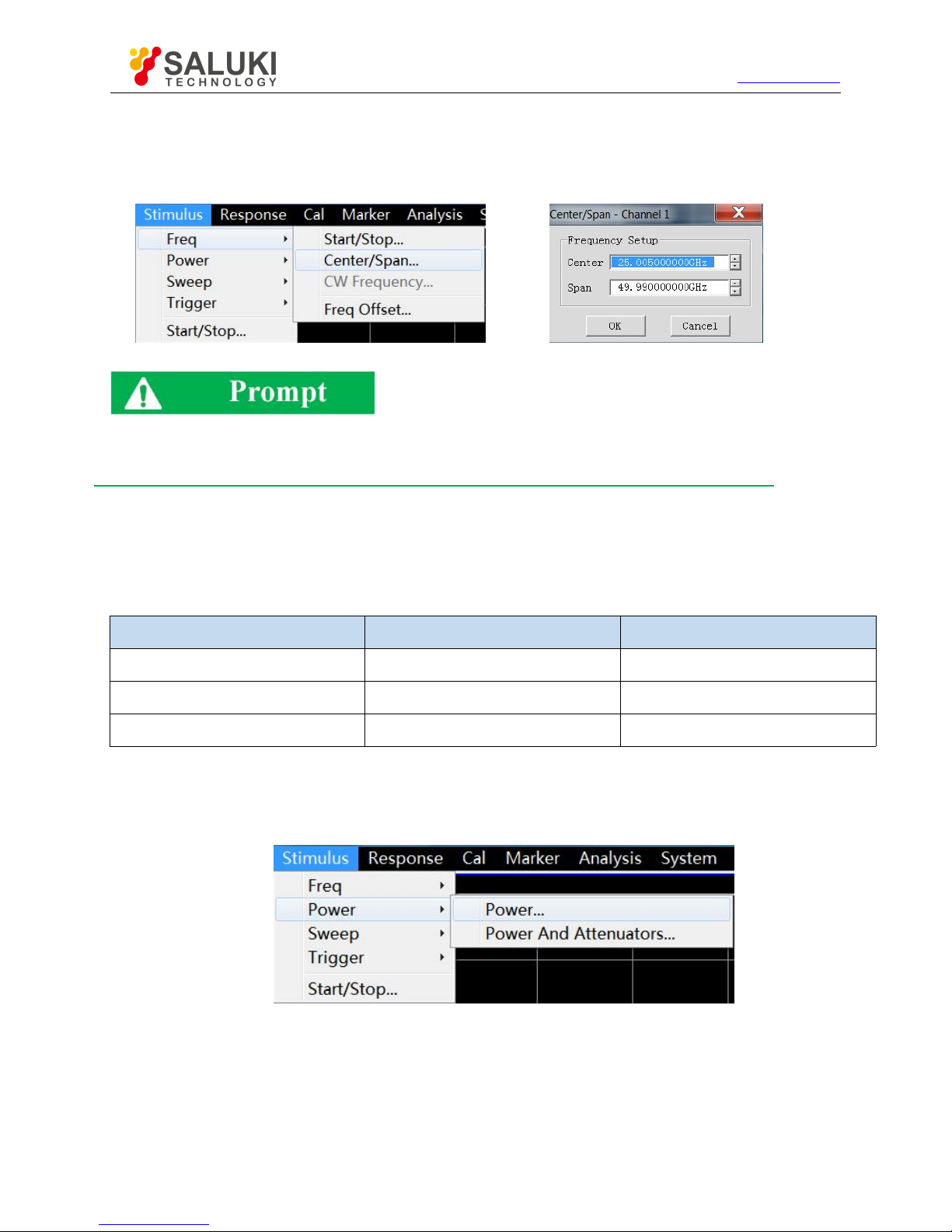
Tel: 886.2.2175 2930 Email: [email protected]
www.salukitec.com
81
Fig. 4.8 Setting of Start / Stop Frequency
3) Setting of center frequency and frequency span
Menu path: [Stimulus] > [Freq]
Fig. 4.9 Setting of Center Frequency and Frequency Span
[Frequency] shortcut key
The frequency can be rapidly set with the [Frequency] shortcut key in the functional key zone of the front panel.
4.4.
Setting of Signal Power Level
The power level refers to the power level of the output signal of the test port. The power level indicators of the port of S3602 series
vector network analyzer are as follows.
Table 4.2 Power Level Indicators of Source Output Signal
Frequency range
Source frequency range (dBm)
Configuration
10MHz-13.5GHz/26.5GHz/43.5GHz/50GHz/67GHz
-30 - +20
Standard configuration
10MHz - 13.5GHz/26.5GHz
-100 - +20
Option: program-controlled step attenuator
10MHz - 43.5GHz/50GHz
-90 - +20
Option: program-controlled step attenuator
1) Setting of power level
Menu path: [Stimulus] > [Power].
[Power] shortcut key is set in the functional key zone of the front panel and the shortcut menu bar.
Page 82
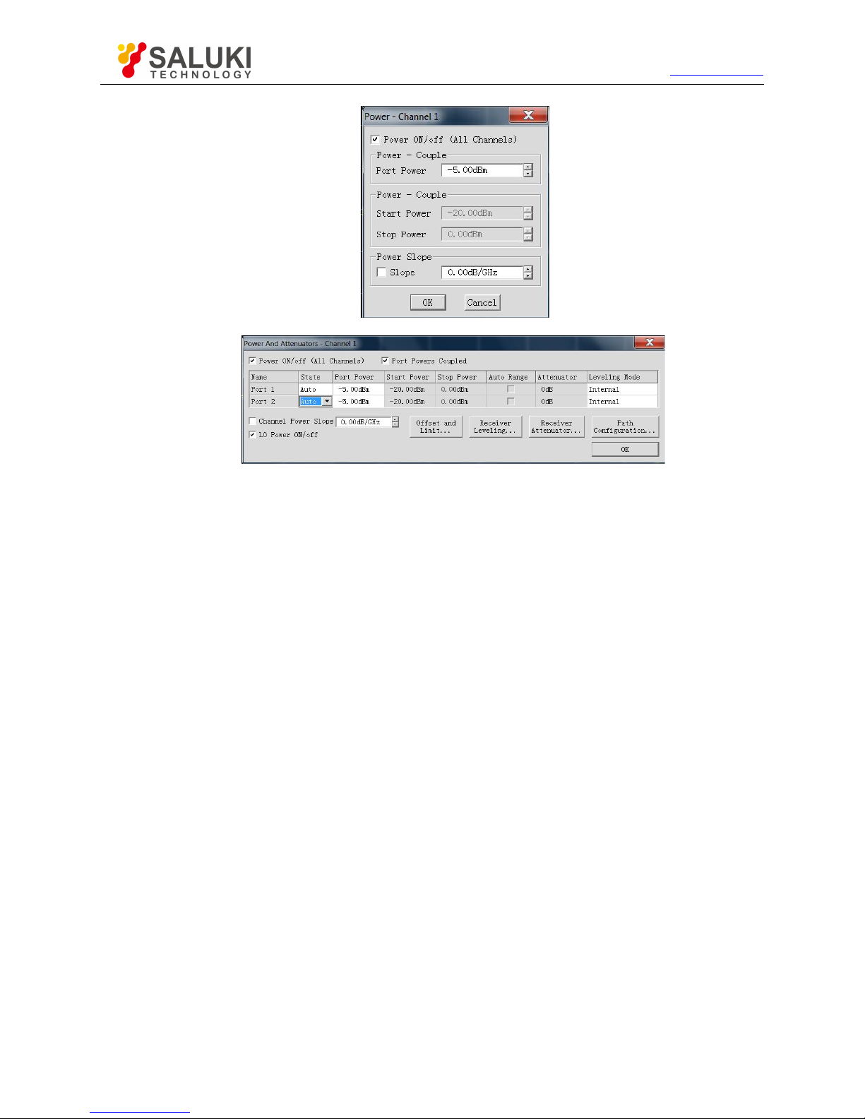
Tel: 886.2.2175 2930 Email: [email protected]
www.salukitec.com
82
Fig. 4.10 Setting of Power Level
2) Cutoff of port power
Menu path: [Stimulus] > [Power] > [Power...].
Or, switch the power by changing the setting of the [Power ON/off] check box in the [Power] dialog box.
3) Manual setting of attenuation
Menu path: [Stimulus] > [Power] > [Power and attenuators...]. The [Power and attenuators] will appear. Click to clear the [Auto
attenuation] zone check box. Click the [Attenuation] input box and enter the attenuation value.
4) Setting of power slope
Menu path: [Stimulus] > [Power] > [Power...]. The [Power] dialog box will appear. Click [Slope] check box. Click the [Slope] input
box and enter the power slope.
5) [Power] dialog box
a) [Power ON/off] check box
If this check box is ticked, the port will normally output the power. If this check box is cleared, the port output power will be cut off.
b) [Power-port 1]
Set the power level of the port 1.
c) [Power slope] check box
Tick the [Power slope] check box and enter the slope value in the [Slope] input box to enable the power slope function.
The power slope is used to compensate the power loss of the cable and test fixture as a result of frequency increase.
If the power slope function is enabled, the output power of the test port will increase (or decrease) with the increase of sweep
frequency.
Unit of power slope: dB/GHz.
Power slope setting range: -2 to +2.
6) [Power and attenuation] dialog box
Page 83

Tel: 886.2.2175 2930 Email: [email protected]
www.salukitec.com
83
a) [Power ON/off] check box
If this check box is ticked, the port will normally output the power. If this check box is cleared, the port output power will be cut off.
b) [Port Powers Coupled] check box
If the [Port Powers Coupled] check box is ticked in the default mode, the power level settings of two ports of the analyzer will be
identical. However, different power levels are required for ports in some measurement applications. For example, the power of
each port must be set separately to measure the gain and reverse isolation of one high- gain amplifier, as the power of the input
port of the amplifier is lower than that of the output port. If the [Port Powers Coupled] check box is cleared, the power level of each
port can be set separately in the analyzer.
c) [State] bar
It is [Auto] in the default mode. In this case, the power ON/OFF state can be switched according to the measurement needs. [ON]
indicates the port power is always ON, while [OFF] indicates the port power is always OFF.
d) [Port power] bar
Set the port power.
e) [Auto Range] bar
If this check box is ticked, any power level can be set within the allowable range of the instrument. If this check box is cleared, the
source power and attenuation can be set manually for certain measurement, such as the reflection amplifier (oscillator or
unsteady-state amplifier) measurement. In this case, the matching source impedance (better than the return loss of 20dB) should
be set within a wide frequency range.
f) [Attenuator] bar
Set the attenuation.
g) [Leveling Mode] bar
Set the fixed amplitude mode, including [Internal], [Receiver] and [Open loop]. The amplitude is not fixed in the [Open loop] mode.
h) [Channel Power slope] check box
Tick the [Slope] check box and enter the slope value in the [Slope] input box to enable the power slope function. The power slope
is used to compensate the power loss of the cable and test fixture as a result of frequency increase.
If the power slope function is enabled, the output power of the test port will increase (or decrease) with the increase of sweep
frequency.
Unit of power slope: dB/GHz.
Power slope setting range: -2 to +2.
i) Attenuator Settings and power range
The programmable attenuator is used to cover the whole power range. It can adjust the power level of the tested device while the
power level of the reference path of the analyzer remains unchanged. Thus, higher accuracy and characteristic indicates and more
accurate matching of source output signals can be realized.
The fully accurate error correction can be done at the power point for measurement calibration. If the power level is changed in the
same attenuator settings as those of measurement calibration, the accuracy of error correction is higher in ratio measurement but
poorer in non-ratio measurement.
4.5.
Setting of Sweep
Sweep refers to the process of continuously measuring data points according to the stimulus values in the specified sequence.
Overview of sweep types
Page 84
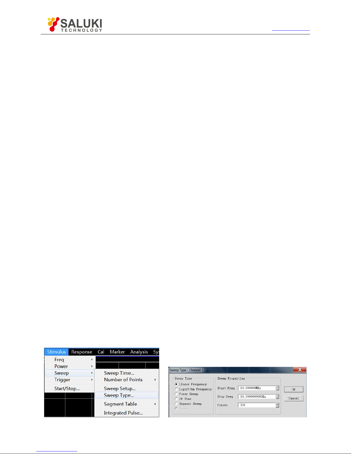
Tel: 886.2.2175 2930 Email: [email protected]
www.salukitec.com
84
Setting of sweep type
Sweep time
Sweep setting
4.5.1.
Overview of Sweep Types
The network analyzer supports six sweep types shown below.
1) Linear frequency
This is the default sweep type of the instrument. The whole frequency range is covered continuously by the frequency linearity.
2) Logarithm frequency
In the logarithmic frequency mode, the source frequency increases in logarithmic steps, and the frequency ratio of every two
adjacent frequency points is identical.
3) Power Sweep
The power is scanned at the point frequency. The maximum sweep range is 50dB. The default frequency sweep range is -30dBm
to +20dBm.
4) CW Time
In the point frequency sweep mode, a single sweep frequency is set in the analyzer, measurement data are accurately and
continuously samples at the intervals determined according to the sweep time and the number of measurement points, and
changes of measurement data with time are displayed.
5) Segment Sweep
Segment sweep aims to start sweep of several segments. The power level, IF bandwidth and sweep time of each segment can be
set independently. After calibration of all segments, one or several segment(s) can be measured according to the calibrations.
Segments are defined according to the frequency increase sequence, and the frequency range must be prevented from
overlapping. The attenuator settings of the power levels of all segments must be identical to prevent damage caused by frequent
switching of the attenuator. If the attenuator settings of the current segment and defined segment are different, the analyzer will
automatically change the power level and attenuator settings of the defined segment.
6) Phase
Scan the phase of one or several source(s) relative to another source. The measured value is -360° to +360°.
4.5.2. Setting of sweep Type
1) Setting of sweep type
Menu path: [Stimulus] > [Sweep] > [Sweep type].
Select the corresponding sweep type in the auxiliary menu bar or in the [Setting of sweep type] dialog box.
Fig. 4.11 Setting of Linear Frequency Sweep Type
Page 85
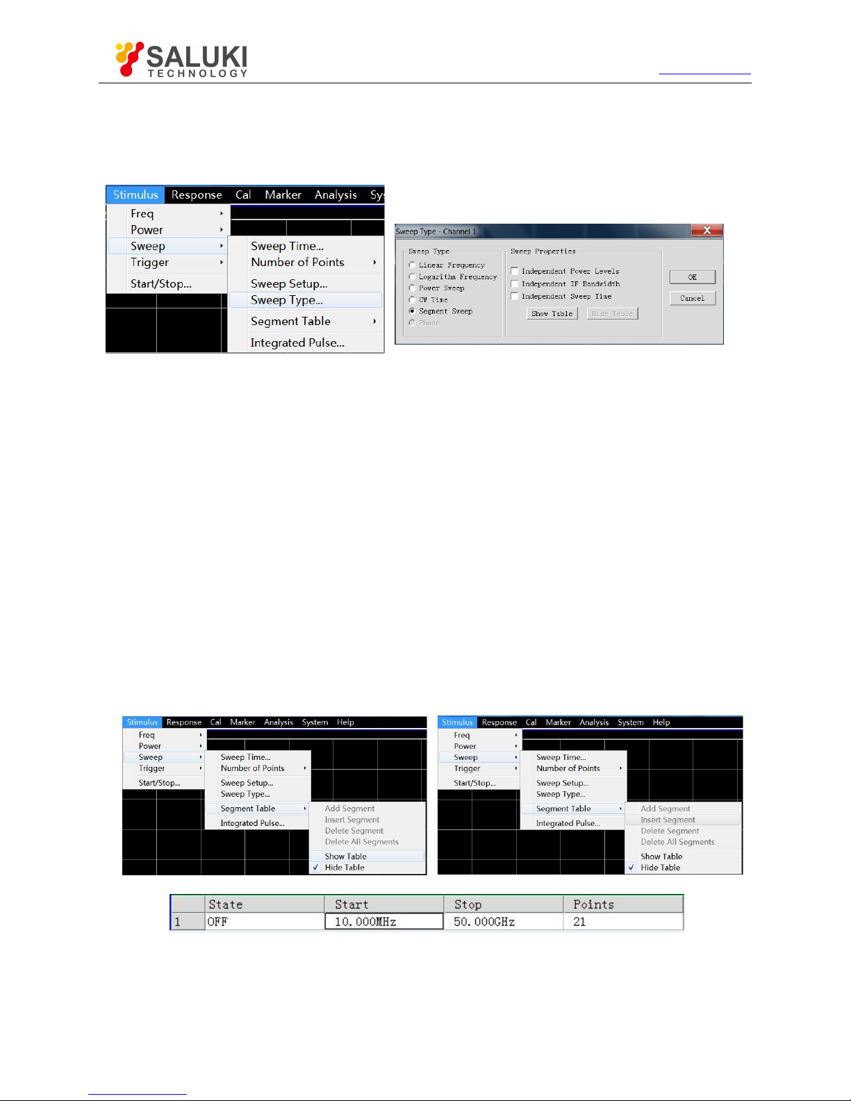
Tel: 886.2.2175 2930 Email: [email protected]
www.salukitec.com
85
2) Setting of segment sweep type
Menu path: [Stimulus] > [Sweep] > [Sweep type].
Auxiliary menu bar: click [Segment sweep] or select [Segment sweep] in the [Setting type] dialog box.
Fig. 4.12 Setting of Segment sweep Type
Dialog box setting instructions:
a) [Independent power levels] check box: tick it to set the independent power level of each segment. In this case, the
attenuator settings must be identical.
b) [Independent IF bandwidth] check box: tick it to set the independent IF bandwidth of each segment.
c) [Independent sweep time] check box: tick it to set the independent sweep time of each segment.
d) [Show table] button: click it to create and edit the sweep table.
e) [Hide table] button: click it to hide the segment sweep table.
3) Segment insertion and deletion
Only the displayed segment table can be edited.
Menu path: [Stimulus] > [Sweep] > [Segment table] > [Display segment table]. The segment table sub- menu will appear.
Tick [Display segment table] in the segment table sub-menu. Click [Insert segment] in the segment table sub- menu to add a new
segment in front of the selected segment. Click [Delete segment] in the segment table sub- menu to delete the selected segment.
Click [Delete all] to delete the whole segment table.
Fig. 4.13 Segment Insertion and Deletion
a) Editing of segment table
b) Double-click the [State] box of the segment and select “ON" or “OFF" to open or close the segment.
c) Double-click the [Starting stimulus] box of the segment and enter the starting frequency of the segment.
Page 86
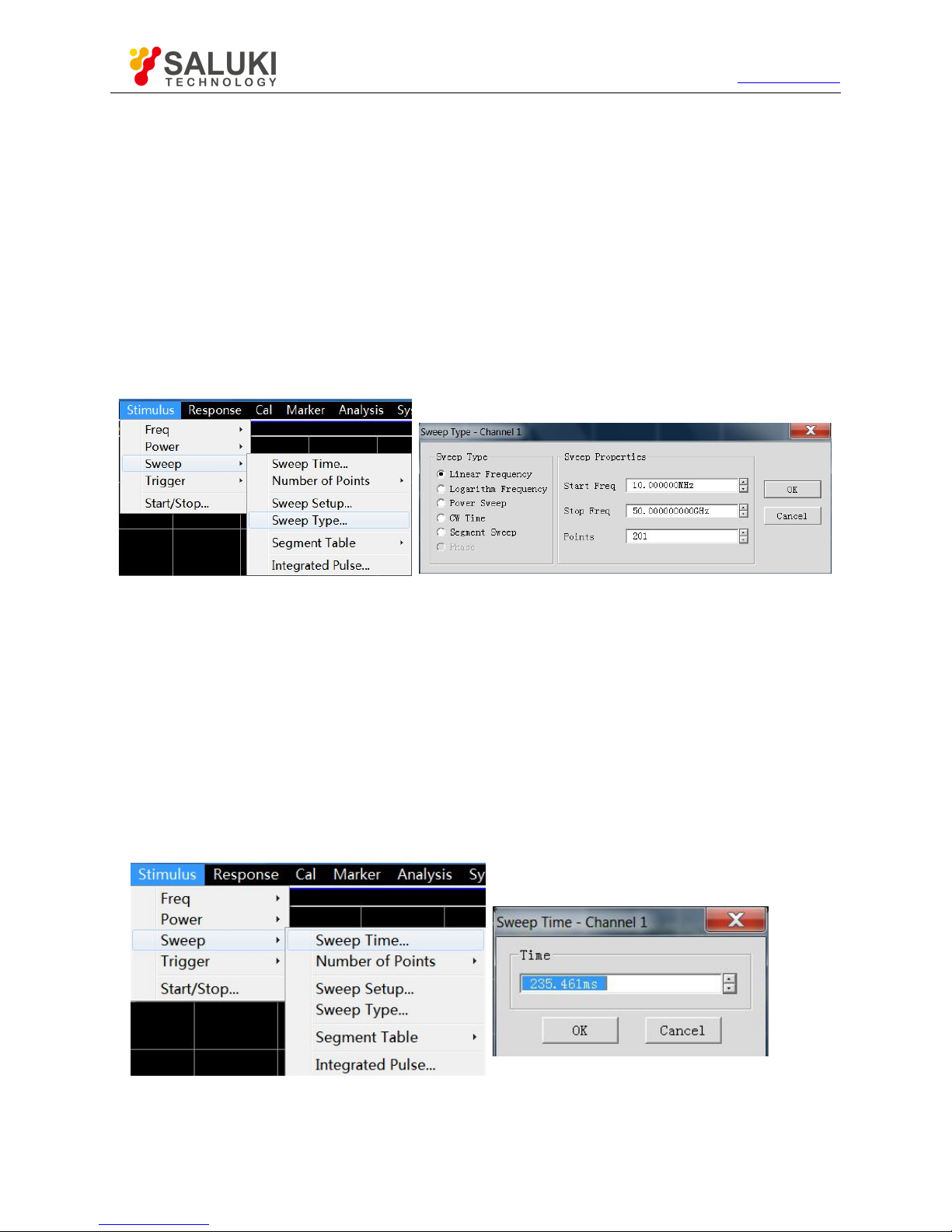
Tel: 886.2.2175 2930 Email: [email protected]
www.salukitec.com
86
d) Double-click the [Ending stimulus] box of the segment and enter the ending frequency of the segment.
e) Double-click the [Number of sweep points] box of the segment and enter the number of sweep points of the segment.
f) Double-click the [Power level] box of the segment and enter the power level of the segment (the independent power level
option is opened).
g) Double-click the [Intermediate frequency bandwidth] box of the segment and enter the IF bandwidth of the segment (the IF
bandwidth option is opened).
h) Double-click the [Sweep time] box of the segment and set the sweep time (the independent sweep time option is opened).
4) Setting of phase sweep type
Menu path: [Stimulus] > [Sweep] > [Sweep type]. The sweep type sub-menu will appear.
Click the phase sweep in the auxiliary menu bar, or select phase sweep in the [Sweep type setting] dialog box.
Fig. 4.14 Setting of Sweep Type
4.5.3.
Sweep Time
After setting of measurement, the minimum sweep time will be adopted by the analyzer. The sweep time can be increased to meet
certain requirements of measurement. If the sweep time is set as 0, the minimum sweep time will be adopted automatically by the
analyzer. If the sweep is no less than 300ms, a sweep indicator will be displayed on the analyzer, indicating the point-to-point
measurement sweep. The measurement indicator is a small upward arrow, showing the point at which measurement is just
completed on the trace.
1) Setting of sweep time
Menu path: [Stimulus] > [Sweep] > [Sweep time...]. The dialog box of sweep time will appear.
Enter the sweep time directly in the [Sweep time] box. For setting of the sweep time with the keys and auxiliary menu bar, directly
enter the sweep time in the input toolbar.
Fig. 4.15 Setting of sweep Time
4.5.4. Setting of sweep
1) sweep setting
Page 87
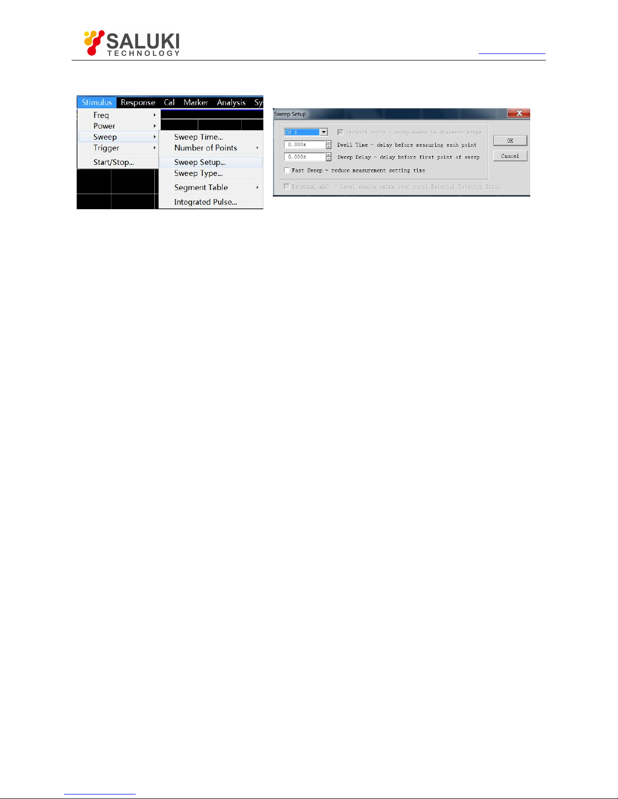
Tel: 886.2.2175 2930 Email: [email protected]
www.salukitec.com
87
Menu path: [Stimulus] > [Sweep] > [Sweep setup...]. The [Sweep setup] dialog box will appear.
Fig. 4.16 sweep Setup
2) [Sweep setup] dialog box
a) [Channel] box
Select the channel applicable to sweep setting.
b) [Stepped sweep] check box
In the stepped sweep mode, the source is tuned to a frequency point and the frequency point is measured after the specified dwell
time. Then the source is tuned to next frequency point. A device of long electrical delay can be accurately measured. If this check
box is cleared, the analyzer may work in the analog sweep or step sweep mode, depending on the setting of the sweep time and IF
bandwidth.
c) [dwell time] input box
Set the dwell time at each point before obtaining the measurement data. This is only applicable to the step scanning mode.
d) [Sweep delay] input box
Set the waiting time of the analyzer before obtaining the measurement data. It refers to the delay before measurement of the first
point.
e) [Quick sweep] check box
If the [Quick sweep] check box is selected, analog sweep will be started. Data are collected in the sweep process, thus reducing
the waiting time of sweep.
4.6.
Trigger Mode
The trigger signal is used to enable measurement sweep of the analyzer. The sweep mode and time to stop sweep and return to
the holding state are determined by trigger settings. The vector network analyzer has high flexibility in trigger setting.
Simple trigger setting
Detailed trigger setting
[Trigger] dialog box
4.6.1. Simple Trigger Setting
Only the trigger mode of the current active channel can be set by simple trigger setting. Menu path: [Stimulus] > [Trigger]. The
trigger sub-menu will appear. Click [Continuous], [Single] or [Hold] in the sub-menu and select the trigger mode.
Page 88
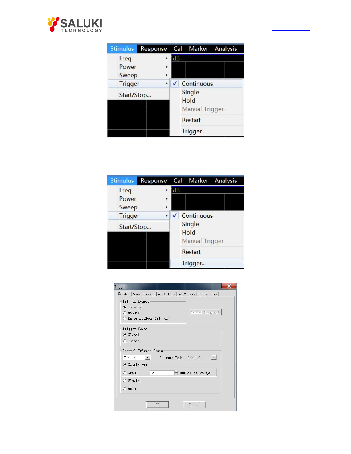
Tel: 886.2.2175 2930 Email: [email protected]
www.salukitec.com
88
Fig. 4.17 Simple Trigger Setting
4.6.2. Detailed Trigger Setting
Menu path: [Stimulus] > [Trigger] > [Trigger...]. The trigger dialog box will appear.
Fig. 4.18 Trigger Sub-menu
Fig. 4.19 Trigger Setting Dialog Box
4.6.3.
[Trigger] Dialog Box
Page 89

Tel: 886.2.2175 2930 Email: [email protected]
www.salukitec.com
89
1) Trigger setting options
a) Trigger source zone
The source of the channel trigger signal is determined by trigger source setting of the trigger source zone. The effective trigger
signal is generated when sweep is not done by the vector network analyzer. Three trigger sources can be selected: internal,
manual and external. The set trigger source will be used as the trigger source of all channels.
[Internal] (default)
a) Trigger signal generation is controlled automatically by the analyzer.
b) One trigger signal is generated immediately after one measurement.
[Manual]
The manual trigger signal is generated in the following methods.
a) Click the [Manual] button in the [Trigger] dialog box.
b) Click the [Manual] item in the [Trigger] sub-menu under the [Stimulus] menu of the menu bar.
[External]
a) The trigger signal is input by [Trig In] of the BNC connector on the rear panel.
b) The signal is TTL level.
c) Level trigger: the high or low level can be set in the [Meas Trigger] dialog box.
d) The pulse duration is 1μs at and must not be longer than the sweep time (otherwise, the trigger may be enabled several
times).
b) Trigger Scope
The measurement channel receiving the trigger signal is determined by trigger range setting. Two types of trigger range can be set:
global and channel.
[Global]
This is the default setting of the analyzer. Except the channel in the holding mode, all channels can receive the trigger signal.
[Channel]
Next channel which is not in the holding mode will receive the trigger signal. After the current channel is measured, next channel
will be selected automatically. Except the channel in the holding mode, all channels will be selected in sequence. The trigger
source should be set in the manual mode to make the above setting effective. Set the [Channel] to enable the spot sweep function.
c) Channel Trigger State
The number of trigger signals to be received by one channel is determined by trigger setting. Four channel triggering states are
provided:
[Continuous]
The channel will receive a number of trigger signals. Sweep will be done continuously.
[Group]
The channel will only receive the trigger signals, the number of which is set in the [Group] input box. Sweep will be done for the set
times, and then the channel will enter the holding mode.
[Single]
The channel will receive one trigger signal. Sweep will be done once, and then the channel will enter the holding
mode.
Page 90

Tel: 886.2.2175 2930 Email: [email protected]
www.salukitec.com
90
[Hold]
The channel will not receive the trigger signal, and sweep will be stopped.
[Spot] ([Trigger mode] check box)
The spot sweep mode can be selected only when the trigger source is manual or external and the trigger range is the channel. In
the spot sweep mode, next data point will be measured in sweep after the channel receives the trigger signal. The channel will
continuously receive the trigger signal until all measurements in the channel are done. Then next channel which is not in the
holding mode will be triggered.
[Channel] ([Trigger mode] check box)
All tracks in the channel will be triggered.
[Sweep] ([Trigger mode] check box)
The sweep trigger mode can be selected only when the trigger source is manual or external and the trigger range is the channel.
The tracks sharing one source port in the channel will be triggered.
2) Meas trigger options
a) Main trigger input zone
Set the nature of the external trigger signal to be received in the trigger input zone.
[Channel trigger delay]
[Delay]: Enter the delay time in the delay input box. When the instrument receives the external trigger signal, sweep will be started
after the delay time.
[Source]
Set the external trigger signal input interface, including the BNC interface and automatic test interface (18-pin).
[Level/edge]
Set the trigger mode of the external trigger signal, including high level, low level, positive edge and negative edge.
[Accept trigger before armed]
If this item is ticked, corresponding sweep will be executed immediately after the vector network analyzer receives the trigger signal;
otherwise, all the received trigger signals will be ignored.
[Ready to receive trigger prompt]
The trigger READY signal is sent by the BNC interface and automatic test interface (21-pin). High level and low level of the signal
are optional.
Page 91
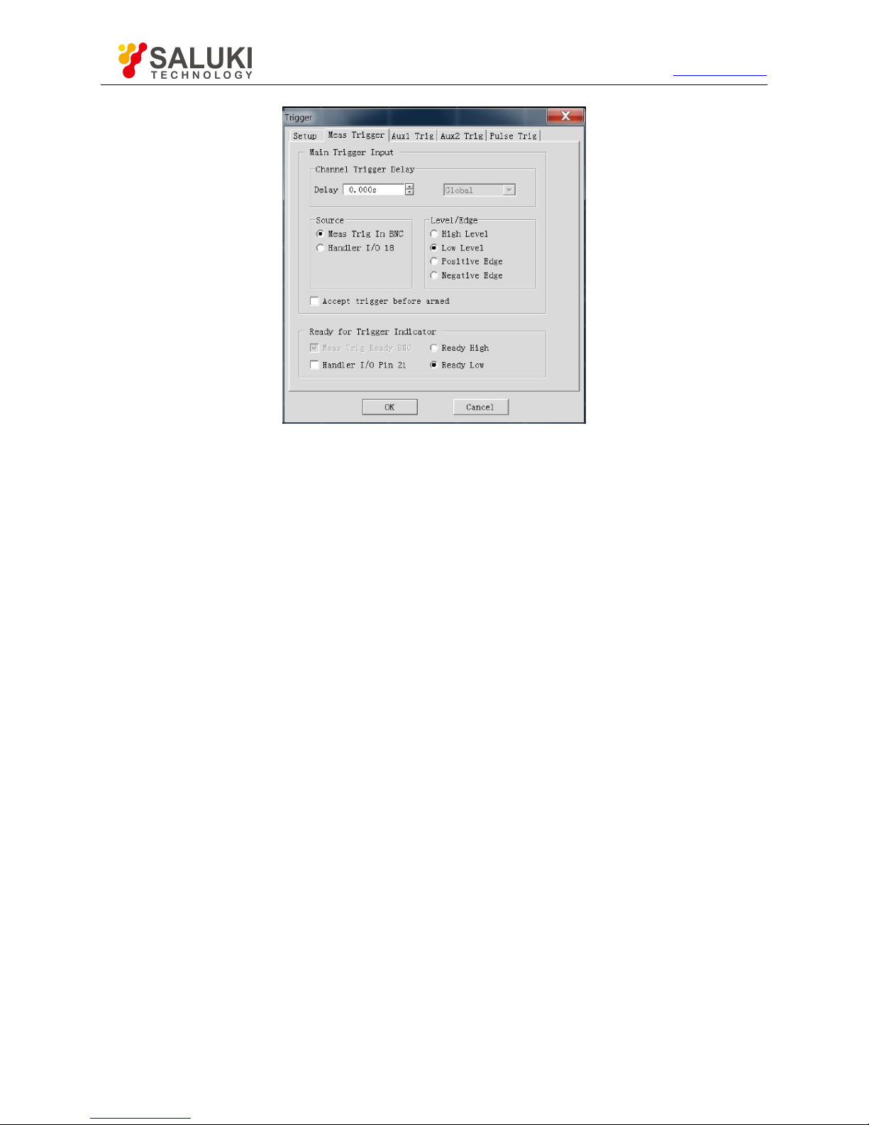
Tel: 886.2.2175 2930 Email: [email protected]
www.salukitec.com
91
Fig. 4.20 Measurement Trigger Dialog Box
3) Auxiliary 1/2 trigger option
a) Auxiliary trigger output zone
[Enabled]
Tick the check box to open the external trigger output of the corresponding channel; otherwise, the external trigger output will be
closed.
[Polarity]
Set the polarity of the trigger output signal in the radio box: [Positive pulse] or [Negative pulse].
[Position]
Set the time to send the trigger output signal in the radio box: [Before data acquisition] or [After data acquisition].
[Pulse Duration]
Input the pulse duration of the trigger output signal in the input box.
[Enable the waiting for external equipment holding signal]
If this check box is ticked, data will not be captured until the vector network analyzer receives the specific level from the auxiliary
trigger input (1&2) connector of the rear panel. This signal indicates that the external device is ready and the network analyzer is
allowed to capture data. Otherwise, the network analyzer will not wait. However, a trigger signal will be sent when the network
analyzer is ready. This signal cannot be used to trigger the network analyzer. It is generated by the internal, manual or external
source.
[Auxiliary trigger input]
When the network analyzer is ready, a confirmation signal will be sent to the auxiliary 1 & 2 connection port. The signal can be in
the rising edge, falling edge, high level or low level form.
[Delay]
When the network analyzer receives the holding signal, data will be captured after the corresponding delay time.
Page 92
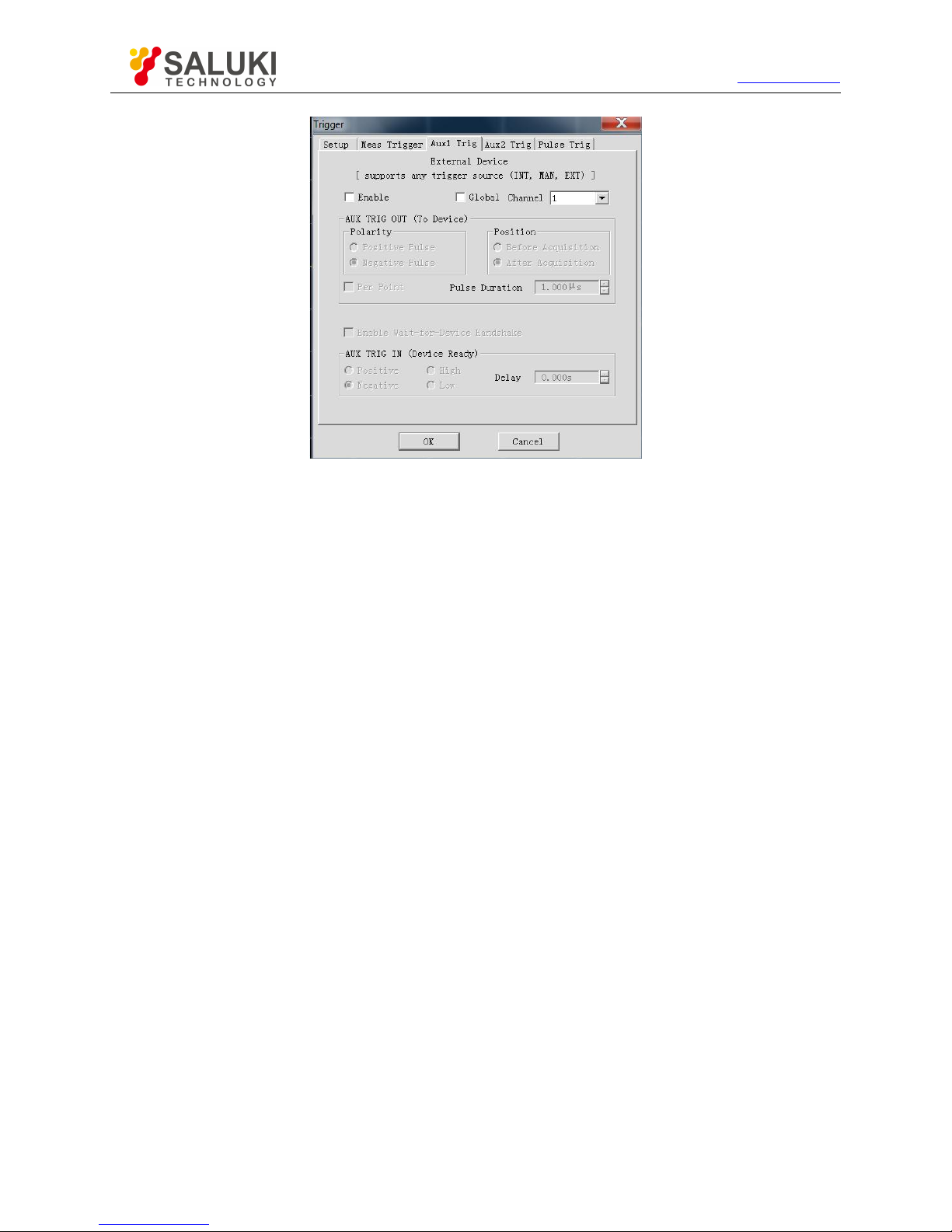
Tel: 886.2.2175 2930 Email: [email protected]
www.salukitec.com
92
Fig. 4.21 Auxiliary 1/2 Trigger Dialog Box
4) Pulse trigger options
a) Synchronous pulse input zone
Select the internal or external source to synchronize the internal pulse generator of the analyzer.
[Pulse trigger option]
Internal: the pulse generator is synchronized according to the periodic signal generated in the analyzer, and the output pulse train
period is determined according to the pulse repetition period in the pulse measurement interface.
External: the pulse repetition period specified by the user is ignored. One pulse train will be output once an effective external pulse
synchronization signal is detected by the analyzer. The delay and width of the pulse generator can be set respectively in the pulse
measurement interface. The external pulse synchronization input signal will be input through the pulse input/output interface of the
rear panel of the analyzer. The configurable synchronization trigger signal can be input to the analyzer according to the pulse
synchronization input signal. If the level is trigger, the analyzer will output a pulse train. If the level is continuously effective, the
analyzer will continue to output another pulse train. If the edge is triggered, the analyzer will be triggered by one effective edge
signal to output a pulse train. The pulse train length is the maximum value (delay + width) in all the enabled pulse generators.
[Level/edge]
Set the characteristics of the effective external pulse synchronization input signal to be received by the analyzer: high level, low
level, rising edge or falling edge.
b) Receiver output zone
[Synchronize receiver to pulse]
It is used to measure the broadband synchronization pulse. When this function is enabled, the pulse generator output and data
collection are allowed to be synchronized.
[Sync Delay]
Set the delay time before collection of AD data.
Page 93
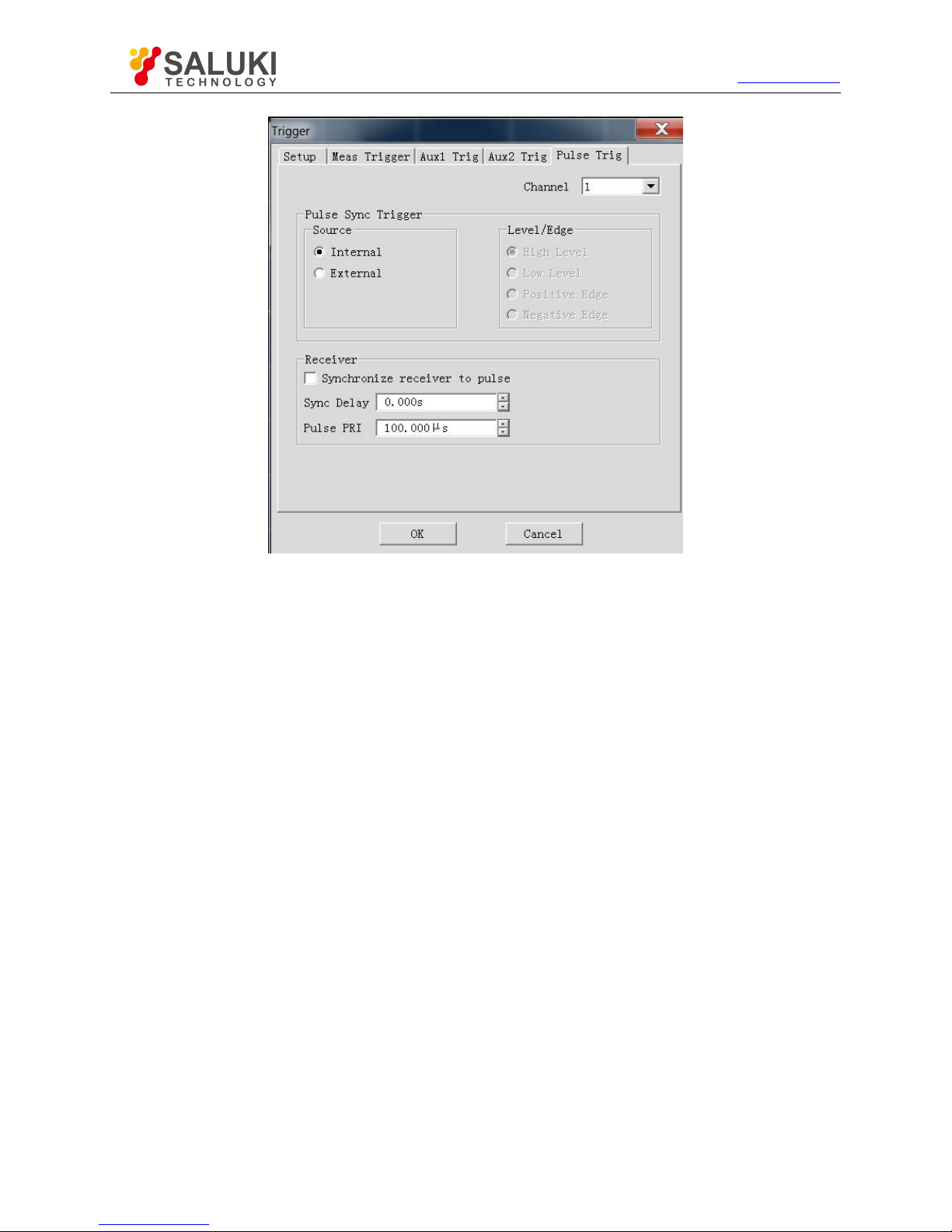
Tel: 886.2.2175 2930 Email: [email protected]
www.salukitec.com
93
Fig. 4.22 Pulse Trigger Dialog Box
4.7.
Setting of Data Format and Scale
The data format refers to the display of measurement data in the graphical form. Select the data format which is the most favorable
to understand the characteristics of the tested device. This section introduces nine data formats and the method of scale setting so
as to better display the measurement information.
Data format
Data format setting
Scale
4.7.1. Data Format
1) Rectangular coordinate format
Seven of nine formats of measurement data are in the rectangular coordinate form. This format is also known as the Cartesian
format, X/Y format or linear format and is suitable to display the frequency response information of the tested device. For example,
the rectangular coordinates in Fig. 4.23 show the following information.
Stimulus value (frequency, power or time) in the linear scale form on the X-axis in the default mode.
Response value corresponding to the stimulus value on the Y-axis.
Page 94
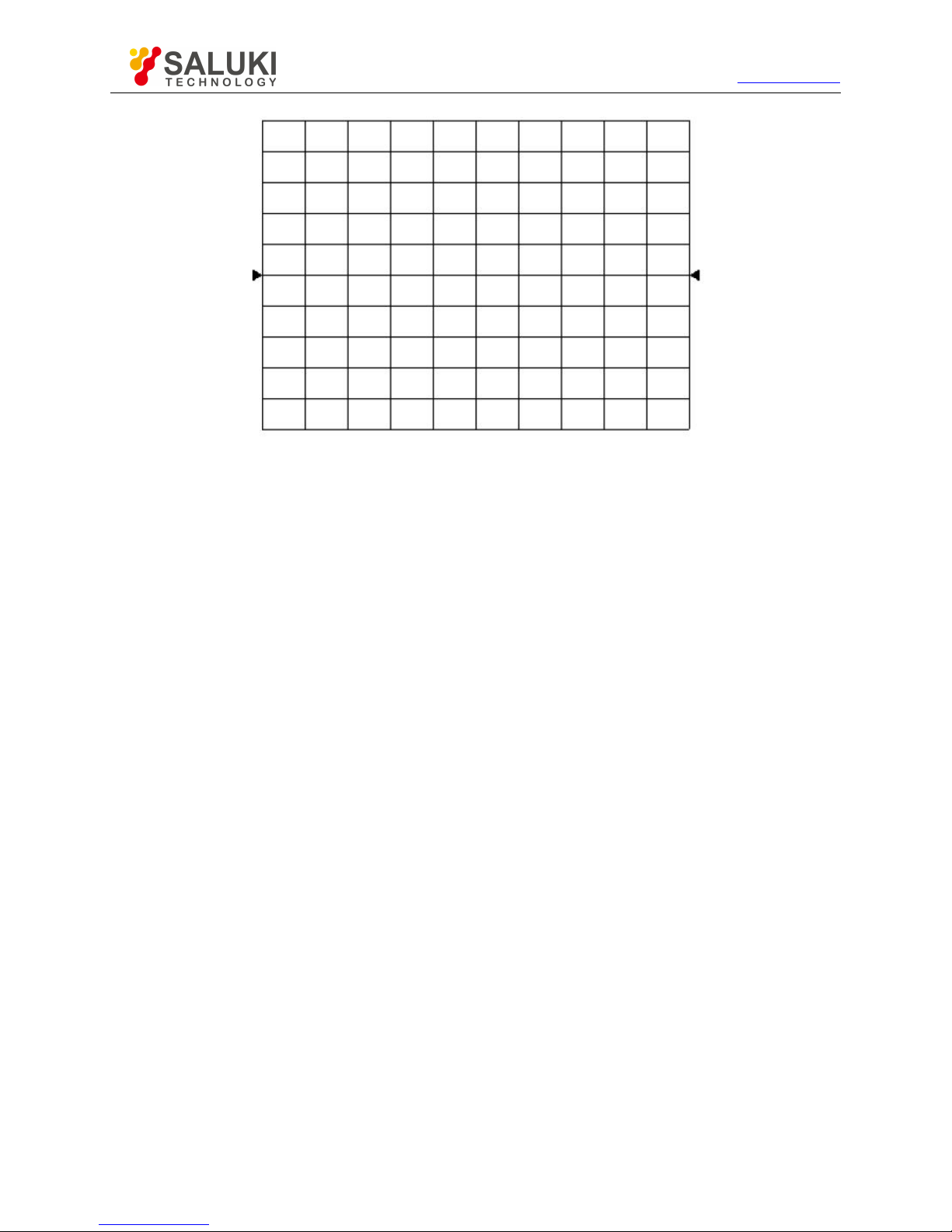
Tel: 886.2.2175 2930 Email: [email protected]
www.salukitec.com
94
Fig. 4.23 Rectangular Coordinate Format
a) Logarithmic amplitude format
Display the amplitude information (no phase information).
Y-axis unit: dB
Applicable typical measurement: return loss, insertion loss and gain.
b) Phase format
Display the phase information (no amplitude information).
Y-axis unit: phase (degree)
Applicable typical measurement: linear phase offset.
c) Group delay format
Display the signal transmission time through the tested device.
Y-axis unit: time (second)
Applicable typical measurement: group delay.
d) Linear amplitude format
Only display the positive value.
Y-axis: no unit (U) in ratio measurement and milliwatt (mW) in non-ratio measurement.
Applicable typical measurement: reflection and transmission coefficient (amplitude) value and time domain transformation
e) Standing wave ratio format
Display the reflection measurement data calculated by the formula (1+ρ)/(1-ρ), where ρ is the reflection coefficient.
Effective in reflection measurement.
Y-axis: no unit.
Applicable typical measurement: standing wave ratio.
f) Real part format
Display the real part of the measurement complex.
Page 95
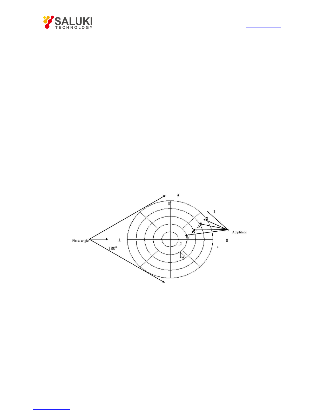
Tel: 886.2.2175 2930 Email: [email protected]
www.salukitec.com
95
It is similar to the linear amplitude format, but both the positive value and negative value can be displayed.
Y-axis: no unit.
Applicable typical measurement: time domain and auxiliary input voltage for maintenance purposes.
g) Imaginary part format
Only display the imaginary part of measurement data.
Y-axis: no unit.
Applicable typical measurement: impedance measurement in design of matching network.
2) Polar coordinate format
The polar coordinate format shown in Fig. 4.24 includes the amplitude and phase information. The vector value can be read in the
following method.
a) The amplitude of any point is determined by the displacement of this point relative to the central point (or zero point). In the
default mode, the amplitude is a linear scale, and the excircle scale is set as 1.
b) The phase of any point is determined by the angle relative to the X-axis.
c) The frequency information can only be read through the marker. The default marker format includes the real part and
imaginary part. The marker dialog box can be opened in the marker/analysis menu. Other formats can be selected in the
advanced marker menu.
Fig. 4.24 Polar Coordinate Format
3) Smith chart format
Smith chart shown in Fig. 4.25 is a tool to map the reflection measurement data of the tested device into impedance.
Each point of the chart represents a complex impedance composed of the real resistance (R) and virtual reactance (±jX). The
resistance, reactance, equivalent capacitance and inductance can be read through the marker.
Page 96
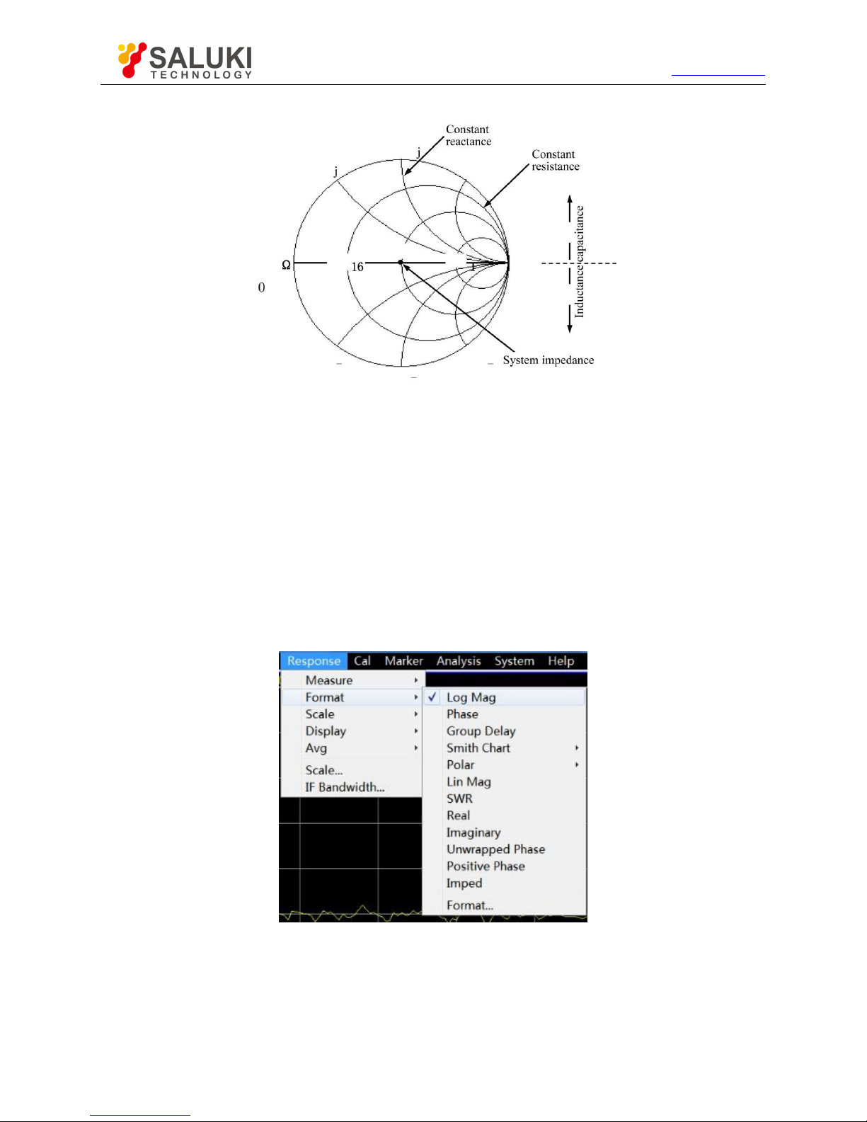
Tel: 886.2.2175 2930 Email: [email protected]
www.salukitec.com
96
Fig. 4.25 Smith Chart Format
a) The horizontal axis of the center of Smith chart represents the pure resistance, and the center of the horizontal axis
represents the system impedance. The leftmost resistance on the horizontal axis is zero, indicating a short circuit. The
rightmost resistance of the horizontal axis is infinite, indicating an open circuit.
b) The points on the intersecting circle of Smith chart and horizontal axis have the same resistance.
c) The points on the tangent of Smith chart and horizontal axis have the same reactance.
d) The reactance of the upper part of Smith chart is positive. Therefore, the upper part is the sensitive zone.
e) The reactance of the lower part of Smith chart is negative. Therefore, the lower part is the capacitive zone.
4.7.2. Data Format Setting
Menu path: [Response] > [Format]. The format sub-menu will pop up.
Fig. 4.26 Setting of Data Format
4.7.3. Scale
The scale refers to the scale of the vertical part of the display grid. In the polar coordinate and Smith chart format, the scale refers
to the full scale of the excircle. The display mode of measurement data on the screen are determined by scale and format settings.
In the log format, the scale setting range is 0.001dB/grid to 500dB/grid.
Page 97
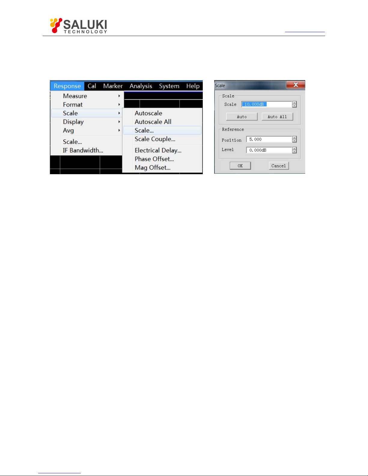
Tel: 886.2.2175 2930 Email: [email protected]
www.salukitec.com
97
1) Scale setting
Menu path: [Response] > [Scale]. The scale sub-menu will pop up.
Set the appropriate scale, reference location and reference level by clicking the corresponding input zone or keys.
Fig. 4.27 Setting of Scale
2) Scale setting dialog box
a) Scale zone
[Scale] box
Enter the set scale value.
[Automatic scale] button
Click the [Automatic scale] button. The analyzer will automatically select the vertical scale to better display the active trace in the
vertical grid of the screen. The stimulus value will not be affected, and only the scale value and reference value are changed.
i.
An appropriate scale factor will be selected so that data are displayed in 80% of the screen.
ii.
The center value of the trace on the screen will be selected as the reference value.
[All automatic scales] button
Click the [All automatic scales] button. The analyzer will select appropriate scales of all tracks in the window so that the tracks are
better displayed in vertical grids of the window.
b) Reference setting zone
[Reference position] button
The reference position refers to the position of the reference line in the rectangular coordinate figure. The position of the bottom
line in the figure is 0, the position of the top line is 10, and the default value of the reference position is 5.
[Reference value] button
The reference value refers to the value of the reference line in the rectangular coordinate format, and the value of the excircle in
the polar coordinate and Smith chart format. The setting range is -500dB to +500dB in the logarithmic amplitude format.
4.8.Observation of Multiple Tracks and Opening of Multiple Channels
A convenient method is provided in the pre-configuration function of the analyzer for multi-trace, multi-channel and multi-window
measurement. The analyzer has four pre-configured Measurement setupss. If one kind of setting is selected, the current trace and
window will be closed, and a new trace and window will be created. The window arrangement of four presettings is as follows.
Page 98
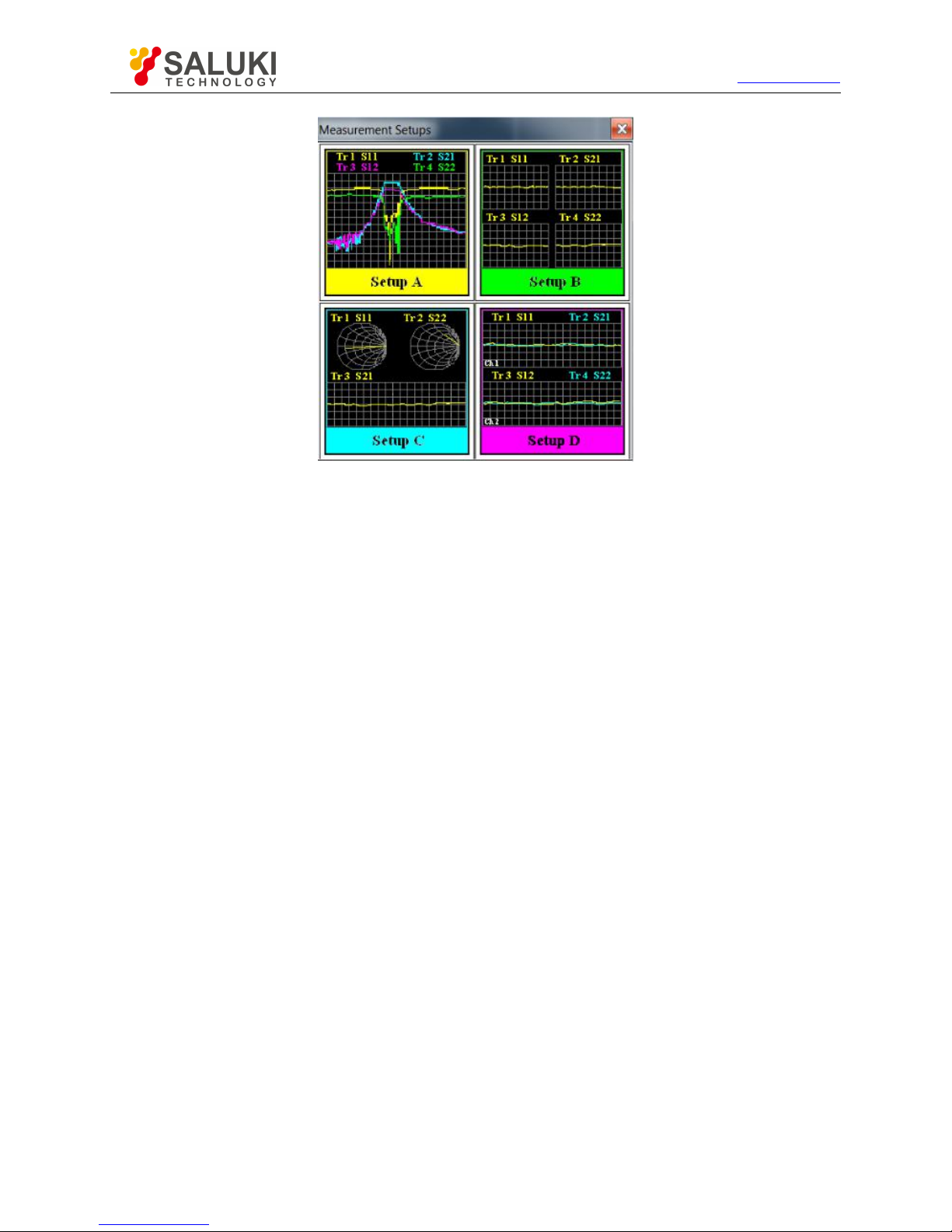
Tel: 886.2.2175 2930 Email: [email protected]
www.salukitec.com
98
Fig. 4.28 Preconfigured Window Arrangement
Setting A
Four tracks will be created in Window 1: S11, S21, S12 and S22, in the logarithmic format in Channel 1.
Setting B
Four tracks will be created in four windows, in the logarithmic format in Channel 1. S11 will be displayed in Window 1, S21 in
Window 2, S12 in Window 3 and S22 in Window 4.
Setting C
Three tracks will be created in three windows of Channel 1. S11 will be displayed in the Smith chart format in Window 1, S22 in the
Smith chart format in Window 2 and S21 in the logarithmic format in Window 3.
Setting D
Four tracks will be displayed in two windows, in the logarithmic format in two channels. S11 and S21 will be displayed in Window 1
of Channel 1, and S12 and S22 in Window 2 of Channel 2.
1) Preconfigured Measurement setups
Menu path: [Response] > [Display] > [Measurement setups...]. The Measurement setups dialog box will appear. Select the
preconfigured Measurement setups in the dialog box.
Page 99
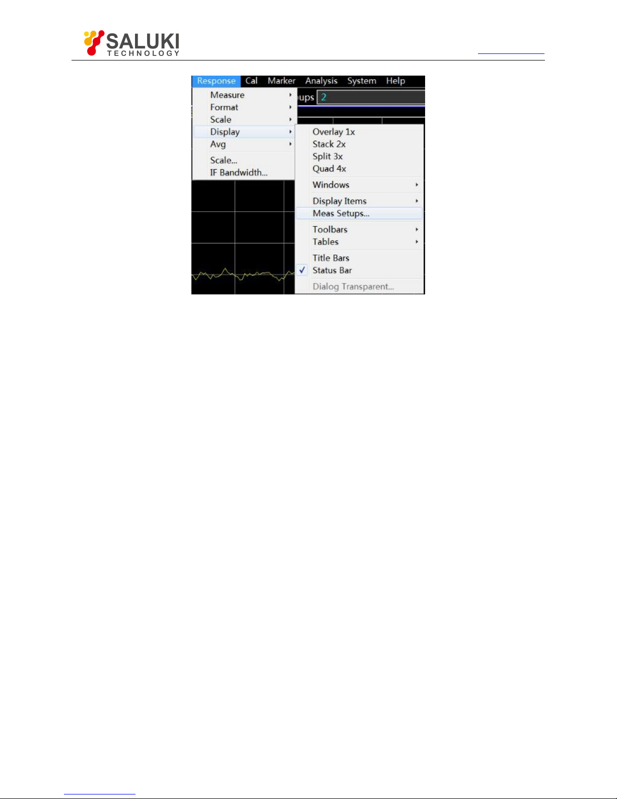
Tel: 886.2.2175 2930 Email: [email protected]
www.salukitec.com
99
Fig. 4.29 Pre-configured Measurement setups
2) Window arrangement
a) Several methods of window adjustment are provided in the analyzer.
Use the mouse to move and adjust the window.
Arrange the windows of the analyzer by the [Tile], [Cascade], [Maximize] and [Minimize] items of the
window menu.
Arrange the windows by the [One-window], [Two-window], [Three-window] and [Four-window] items of the display menu.
Use the [Minimize], [Maximize/reduce down] and [Close] button in the top right corner of the window to adjust or hide the
window.
b) The display menu of the analyzer provides four kinds of window arrangement. The existing tracks are distributed into different
windows according to a certain algorithm.
One-window arrangement
All tracks are displayed in one window in a cascading manner.
Two-window arrangement
All tracks are displayed in two windows which are vertically overlapped.
Three-window arrangement
All tracks are displayed in three windows. Two of the three windows are arranged in the upper part, and the other in the lower part.
Four-window arrangement
All tracks are displayed in four windows which respectively cover one fourth of the screen.
c) Setting of window arrangement
Menu path: [Response] > [Display]. The display sub-menu will pop up. Select the window arrangement mode in the display
sub-menu.
Page 100
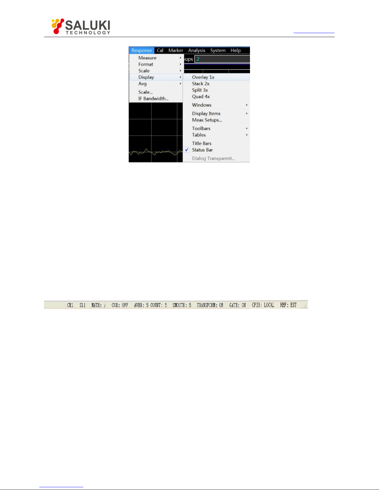
Tel: 886.2.2175 2930 Email: [email protected]
www.salukitec.com
100
Fig. 4.30 Setting of Window Arrangement
4.9.
Setting of Analyzer Display
You can use the display menu of the analyzer to display or hide the display elements and customize the screen. These display
elements are usable for measurement observation, setting and modification, including the status bar, toolbar, list, measurement
display, data trace, memory trace and title bar.
Status bar
Toolbar
Table
Display contents
Title bar
4.9.1.
Status Bar
1) The opened status bar will be displayed at the bottom of the screen, including the following contents:
Current active channel
Measurement parameter of active trace
Mathematical operation of active trace
Error correction status of active trace
If the average function is enabled, the average factor of the current active channel and the average times will be displayed.
If the smoothing function is enabled, the number of smoothing points will be displayed.
If the function of time domain transformation is enabled, "TRANSFORM: ON" will be displayed.
If the gate setting function is enabled, "GATE: ON" will be displayed.
GPIB status: LOCAL or REMOTE.
Reference (REF) signal status: INT or EXT
2) Display of trigger status bar
Menu path: [Response] > [Display]. Tick [Status bar] in the display sub-menu to open the status bar display and clear [Status bar]
 Loading...