Rosemount NGA 2000 TFID Hydrocarbon Analyzer Module SW 3.7 Supplement to SW 3.4 Software-1st Ed. Manuals & Guides

Instruction Manual

HAS55E03IM11S 11/2003

Software Version 3.7.x

Supplement to Software Manual 3.4.x

NGA 2000 Software Manual for TFID Analyzer and Analyzer Module (combined with NGA 2000 Platform, MLT, CAT 200 or TFID Analyzer)

www.EmersonProcess.de

TFID Software 3.7.x Instruction Manual

HAS55E03IM11S

11/2003

ESSENTIAL INSTRUCTIONS

READ THIS P AGE BEFORE PROCEEDING!

Emerson Process Management (Rosemount Analytical) designs, manufactures and test s its products to meet many national and international standards. Because these instruments are sophisticated technical products, you MUST properly install, use, and maintain them to ensure they continue to operate within their normal specifications. The following instructions MUST be adhered to and integrated into your safety program when installing, using and maintaining Emerson Process Management (Rosemount Analytical) products. Failure to follow the proper instructions may cause any one of the following situations to occur: Loss of life; personal injury; property damage; damage to this instrument; and warranty invalidation.

• Read all instructions prior to installing, operating, and servicing the product.

• If you do not understand any of the instructions, contact your Emerson Process

Management (Rosemount Analytical) representative for clarification.

• Follow all warnings, cautions, and instructions marked on and supplied with the product.

• Inform and educate your personnel in the proper installation, operation, and

maintenance of the product.

• Install your equipment as specified in the Installation Instructions of the appropriate

Instruction Manual and per applicable local and national codes. Connect all products

to the proper electrical and pressure sources.

• T o ensure proper performance, use qualified personnel to install, operate, update, program, and maintain the product.

• When replacement parts are required, ensure that qualified people use replacement parts specified by Emerson Process Management (Rosemount Analytical). Unauthorized parts and procedures can affect the product’s performance, place the safe operation of your process at risk, and VOID YOUR W ARRANTY. Look-alike substitutions may result in fire, electrical hazards, or improper operation.

• Ensure that all equipment doors are closed and protective covers are in place, except when maintenance is being performed by qualified persons, to prevent electrical shock and personal injury.

The information contained in this document is subject to change without notice. Misprints reserved.

Emerson Process Management GmbH & Co. OHG

Industriestrasse 1 D-63594 Hasselroth Germany T +49 (0) 6055 884-0 F +49 (0) 6055 884-209 Internet: www.EmersonProcess.com

Software 3.7.x – Supplement to Software 3.4.x and 3.6.x

Addendum for Software Revision 3.6.x to 3.4.x

This chapter describes some important features / changes implemented in software revision 3.6.x, shipped with the newest versions of Fisher-Rosemount NGA gas analyzers and has to be used in combination with the software 3.4.x manual.

1. Display Controls Menu

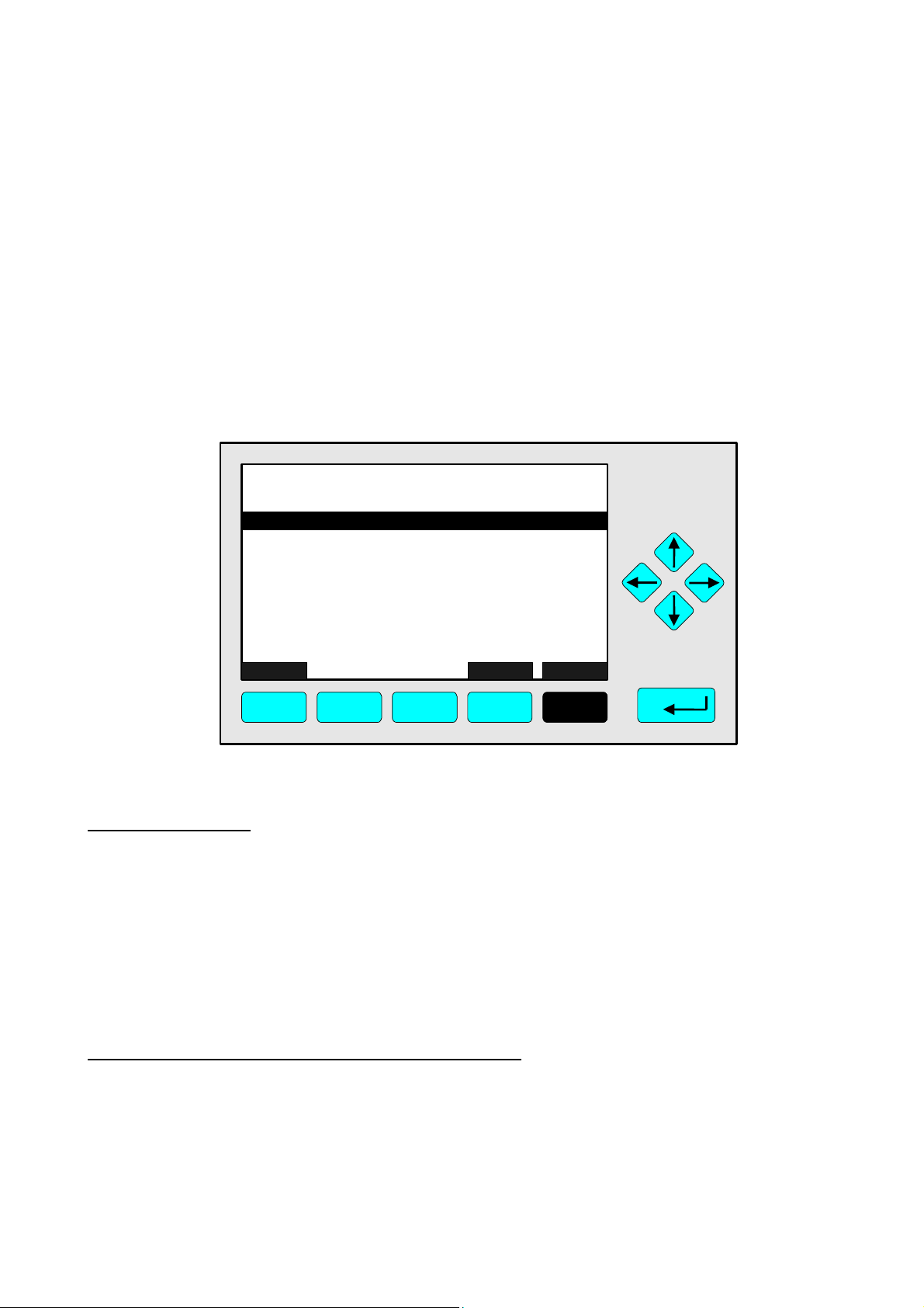
The Display Controls menu (see chapter 7) now has additional menu lines:

Setting parameters:

TAG

-- Display Controls --

Brightness:

Contrast:

Display measurement menu after: 10 Min

Default measurement menu:

Switch off backlight after:

Measure

F1

Single component

F2

F3 F4 F5

Back... More...

37.50 ppm

74 %

23 %

10 Min

♦ Select any line of variables using the ↓ -key or the ↑ -key. ♦ Select the variable using the ↵ -key or the → -key. ♦ Change the whole value using the ↑ -key or the ↓ -key

or select single digits using the ← -key or the → -key and enter a new value using the ↑ -key or the ↓ -key.

♦ Confirm the new value using the ↵ -key or

cancel and return to the previous value using the F2 -key.

Line of variables "Display measurement menu after:"

The value entered in this line defines the time to expire without operator input before the display automatically returns to the measurement display. Options: 10 s, 30 s, 1 min, 5 min, 10 min, 30 min, Never.

HAS55E03IM11S [NGA-e (TFID Software 3.4.X addendum)] 11/03

NGA 2000

A - 1

Line of variables "Default measurement menu:"

Use this line to select the display the analyzer returns to when the time entered in line “display measurement menu after:” has expired. Options: Single Component (Display) or Multi Component (Display)

Line of variables "Switch off backlight after:"

The value entered in this line defines the time to expire without operator input before the backlight is switched off automatically. Using this function saves energy and expands the backlight’s lifetime. Options: 10 s, 30 s, 1 min, 5 min, 10 min, 30 min, Never.

A - 2

NGA 2000

HAS55E03IM11S [NGA-e (TFID Software 3.4.X addendum)] 11/03

Addendum for Software Revision 3.6.x to 3.4.x

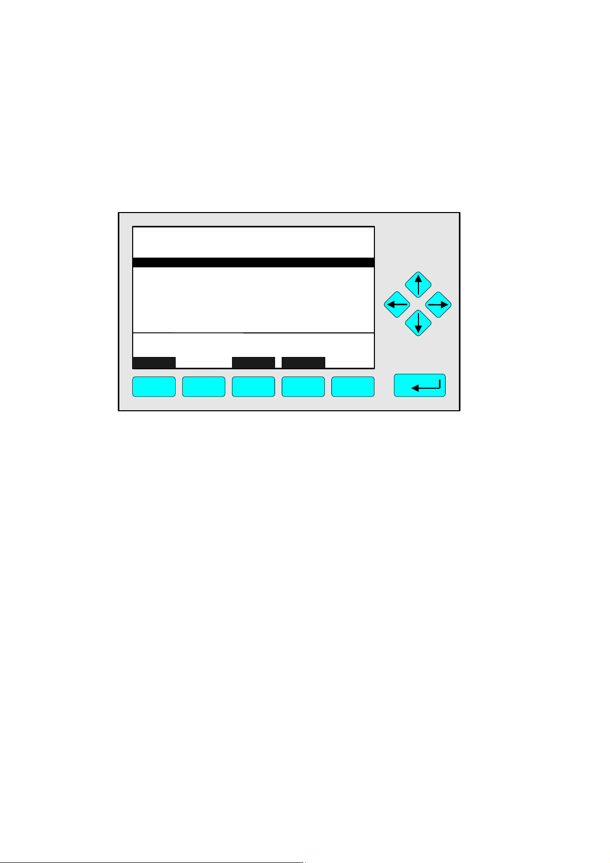
2. Analyzer Basic Controls (calibration) & Setup Menu

One line was added to this menu (see chapter 4.4, p. 4-19):

Function Line "Undo last zero & span calibration !"

TAG

-- Analyzer Basic Controls (calibration) & Setup --

Calibration procedure state..

Start zero calibration procedure ! Start span calibration procedure ! Check calibration deviation:

Undo last zero & span calibration ! Range number: Span gas: Range upper limit:

Operation status:

Measure Status... Channel Back...

F1 F2 F3 F4 F5

37.50 ppm

Disabled

1

46.00 ppm

50.00 ppm Ready

Valves...

Use this function to reset an analyzer’s calibration values to default factory settings if the last calibration procedure has been completed with a poor result due to wrong settings and the calibration is in an undefined status.

Depend on the “Measurement Display Configuration” settings a screen may appear asking for confirmation prior to executing the function (see chapter 3.7, p. 3-6 and chapter 5.1.8, p. 5-49).

HAS55E03IM11S [NGA-e (TFID Software 3.4.X addendum)] 11/03

NGA 2000

A - 3

3. Tolerances Menu

The stability tolerance range 1 … 4 lines of the menu Tolerances (see chapter 5.1, p. 5-8) have been moved into a new menu within the service level:

The stability tolerance function is still enabled but not longer operator definable. Factory setting for all 4 values (ranges 1 … 4) is 10 %.

TAG

-- Tolerances --

Max. zero calibration deviation: 20.00 %

Max. span calibration deviation: 20.00 % Check calibration deviation:

Last zero calibration: Last span calibration:

Measure Channel Back...

F1 F2 F3 F4 F5

95.00 ppm

Disabled

Success Success

A - 4

NGA 2000

HAS55E03IM11S [NGA-e (TFID Software 3.4.X addendum)] 11/03

Calculator on Control Module Level

(Platform, TFID, MLT or CAT 200 Analyzer)

1 SYSTEM CALCULATOR (ON CONTROL MODULE LEVEL)........................................................................2

1.1 P

1.2 L

1.3 CONSTANT VALUES......................................................................................................................................5

1.4 M

1.5 MENU TREE FOR THE SYSTEM CALCULATOR ..................................................................................................6

2 DISPLAY CALCULATOR RESULTS ON MINI-BARGRAPH.......................................................................11

2.1 D

2.2 A

3 ASSIGNMENT TO SIO ANALOG OUTPUTS ...............................................................................................14

RINCIPLE OF PROGRAM SET-UP ..................................................................................................................2

IVE VALUES (REAL MEASURING VALUES) ......................................................................................................4

EMORY VALUES.........................................................................................................................................5

1.5.1 Submenu 'Signals' .................................................................................................................................7

1.5.2 Submenu 'Programming' .......................................................................................................................9

ISPLAY MODE ..........................................................................................................................................11

SSIGN SIGNALS AND CONVENIENT NAMES ..................................................................................................12

PICTURE 1-1: SYSTEM CALCULATOR MENU.................................................................................................................6

P

ICTURE 1-2 : SIGNAL ASSIGNMENT OF SYSTEM CALCULATOR ....................................................................................7

PICTURE 1-4: CONSTANT VALUES ASSIGNMENT ..........................................................................................................9

PICTURE 1-5: PROGRAMMING THE SYSTEM CALCULATOR ..........................................................................................10

P

ICTURE 2-1: MEASUREMENT DISPLAY SET-UP.........................................................................................................11

PICTURE 2-2: PLATFORM SELECTED SIGNAL ASSIGNMENT .........................................................................................12

PICTURE 2-3: LISTING OF ASSIGNED SIGNALS............................................................................................................13

TABLE 1-1: THE OPERATORS OF THE SYSTEM CALCULATOR ........................................................................................3

TABLE 1-2: LIVE VALUES POOL...................................................................................................................................4

HAS55E03IM11S(1) [NGA-e (TFID software 3.7.x)] CM Calculator Page 1

Calculator on Control Module Level

1 System Calculator (on Control Module Level)

1.1 Principle of program set-up

As it would be a too high effort to realize a comfortable mathematical formula system we created a syntax which is easy to input and easy to realize. As we assume that customers or service people have to set-up the program only one times for an installed system it should be acceptable to realize a form which is only done by inputting numbers.

Therefore we have mainly to differ between positive and negative numbers. The program operations are assigned with negative numbers. The operands which are used by these input operations are positive numbers. These positive numbers symbolize signals which are part of a signal pool.

Also we have to know that there are used different classes of operands. That means we have different classes of signal pools.

Those are:

• Live values (real measuring values)

• Constant values

• Memory values.

In each of these classes exists an own numbering and we determine by the operator itself which class of these operands is meant.

Remark:

Opposite to former versions allowing calculator function within ONE TFID/MLT/CAT 200 analyzer module (AM) or for ONE TFID/MLT analyzer (or CAT 200 analyzer resp.) ONLY now the system calculator is based on the C

ontrol Module level (CM). This allows to include ALL analyzer modules resp. MLT channels of a NGA 2000 analyzer system into the calculation. The results of the system calculator can be put onto the 2-8 analog outputs of the programmable Input/Output Module SIO. The SIO as a Control Module I/O is then located in a platform or in a TFID, MLT or CAT 200 Analyzer.

HAS55E03IM11S(1) [NGA-e (TFID software 3.7.x)] CM Calculator Page 2

Calculator on Control Module Level

In the following table we find all the currently available operators (negative numbers) and their meaning. Hereby is used the acronym "IR" for the actually calculated intermediate result of the program.

Table 1-1: The Operators of the System Calculator

Operator number

-10 SUBM m subtract following memory value operand from IR (IR = IR – m)

-11 DIVM m divide IR by following memory value operand (IR = IR / m)

-12 MULM m multiply IR with following memory value operand (IR = IR * m)

-13 STOM m store IR at following memory value and set IR = 0.0 (m = IR; IR = 0)

-14 STOR r store IR to following result and set IR = 0.0 ( r = IR; IR = 0)

-15 NOP no operation (placeholder)

-16 ABS convert IR into absolute value (IR = |IR|)

-17 EOP end of program

-18 SQRT

-19 NEG negate IR (IR = -IR)

-20 INC increment IR (IR = IR + 1)

-21 DEC decrement IR (IR = IR – 1)

-22 INV invert IR (IR = 1 / IR)

-23 EXP exponential function (IR = eIR)

-24 POWM IR raised to the power of the following memory value operand

-25 IF> m1 m2 m3 if IR > 1st following memory value

-26 IF< m1 m2 m3 if IR < 1st following memory value

-27 IF= m1 m2 m3 if IR = 1st following memory value

-28 LN natural logarithm (IR = ln(IR))

-29 LOG base 10 logarithm (IR = log(IR))

Acronym Description

-1 ADD l add following live value operand to the IR (IR = IR + l)

-2 SUB l subtract following live value operand from IR (IR = IR – l)

-3 DIV l divide IR by following live value operand (IR = IR / l)

-4 MUL l multiply IR with following live value operand (IR = IR * l)

-5 ADDC c add following constant value operand to the IR (IR = IR + c)

-6 SUBC c subtract following constant value operand from IR (IR = IR – c)

-7 DIVC c divide IR by following constant value operand (IR = IR / c)

-8 MULC c multiply IR with following constant value operand (IR = IR * c)

-9 ADDM m add following memory value operand to the IR (IR = IR + m)

build square root of IR (IR = √IR)

(IR = IR

then IR = 2 else IR = 3

m

)

nd

following memory value

rd

following memory value

nd

following memory value

rd

following memory value

nd

following memory value

rd

following memory value

HAS55E03IM11S(1) [NGA-e (TFID software 3.7.x)] CM Calculator Page 3

Calculator on Control Module Level

1.2 Live values (real measuring values)

In the platform calculator we have a signal pool of momentary up to 25 possible live signals. The first 10 signals in this pool are fix assigned the rest of the signals are free assignable.

Table 1-2: Live Values Pool

Number Assignment assignment type Signal 1 Result 1 fixed

Signal 2 Result 2 fixed Signal 3 Result 3 fixed Signal 4 Result 4 fixed Signal 5 reserved fixed Signal 6 reserved fixed Signal 7 reserved fixed Signal 8 reserved fixed Signal 9 reserved fixed Signal 10 reserved fixed Signal 11 MLT 1/CH1 Concentration programmable Signal 12 TFID Concentration programmable Signal 13 MLT 2/CH3 Temperature programmable Signal 14 TFID Temperature programmable Signal 15 not assigned programmable

.... ........... programmable

Signal 25 not assigned programmable

By using these numbers of the signal pool we determine the live value operands in the calculator's program.

Example of a calculator program with upper signal assignment:

Result 1 = (MLT 1/CH1 Concentration) + (TFID Concentration)

Step (o+1) -1 ADD (at beginning the intermediate result IR = 0) Step (o+2) 11 Signal 11 (here: MLT1/CH1 Concentration) Step (o+3) -1 ADD Step (o+4) 12 Signal 12 (here: TFID Concentration) Step (o+5) -14 Store IR to result Step (o+6) 1 Result 1 Step (o+7) -17 End of program

HAS55E03IM11S(1) [NGA-e (TFID software 3.7.x)] CM Calculator Page 4

Calculator on Control Module Level

1.3 Constant values

The same principle is used for the constant values. We have a pool of free assignable constant values.

Example of a constant signal pool:

Number Assignment Constant-1 1.000000

Constant-2 10.00000 Constant-3 100.0000 Constant-4 1000.000 Constant-5 10000.00

.... ...........

Constant-21 500.0000

By using the numbers of the signal pool we determine again the constant operands in the calculator's program.

Example of a calculator program with upper live signal and constant assignment:

Result1 = (MLT 1/CH1-Concentration) + 100

Step (o+1) -1 ADD (addition by using the live operand's class) Step (o+2) 11 Live value number 11 (here: MLT1/CH1-Concentration) Step (o+3) -5 ADDC (addition by using the constant operand's class) Step (o+4) 3 Constant number 3 (here: 100.0) Step (o+5) -14 Store IR to result Step (o+6) 1 Result 1 Step (o+7) -17 End of program

1.4 Memory values

The same principle as in constant values is used again for the memory values. We have a pool of usable memory places where intermediate calculation results can be stored to.

HAS55E03IM11S(1) [NGA-e (TFID software 3.7.x)] CM Calculator Page 5

Calculator on Control Module Level

1.5 Menu tree for the system calculator

The following pictures show the menu tree and the LON variables which are assigned to the single menu lines.

System configuration and diagnostics...

↓

System calculator...

↓

- System calculator-

Programming... Signals... Units... Scaling... Calculator is: Enabled Program error in step: 0 Result Calculator 1: 0.1234 Result Calculator 2: 1234.5 Result Calculator 3: 123.45 Result Calculator 4: 98.765

Picture 1-1: System Calculator Menu

With the 'Calculator is' parameter we show whether the system calculator functionality is

• Disabled

• Enabled

• has a Program Error (after trying to enable)

In the case of a program error by the 'Program error in step:' parameter is displayed in what step of the program this error happened. If there is no error this parameter equals '0'.

CALCSTATUS CLCERRLINE CALC1RESULT CALC2RESULT CALC3RESULT CALC4RESULT

HAS55E03IM11S(1) [NGA-e (TFID software 3.7.x)] CM Calculator Page 6

Calculator on Control Module Level

1.5.1 Submenu 'Signals'

The live values' signal assignment is done in the submenu 'Signals...".

System configuration and diagnostics...

↓

System calculator...

↓

Signals...

↓

- Signals -

Signal number: 11

Choose signal source module...

Choose signal...

Signal name: Concentration Signal comes from: MLT/CH1 Current signal value: 123.45 ppm

View...

Picture 1-2 : Signal Assignment of System Calculator

CALCSIGNUMC

CALCSRCSEL_

CALCSIGSEL_

CALCSIGC CALCSRCC CALCVALC

fct3: CASIGLST_

The single signals of the pool (selected by 'Signal number') are assigned by first selecting the source analyzer module (AM) resp. analyzer channel of the requested signal and then the signal name itself. Please, note that is only possible to modify the programmable type of signal numbers.

To realize the signal name's selection there is used an already implemented feature of the AMs. It has being used for the small bar graphs display and for the analog outputs of the SIO module. It is the SVCONT/SVNAME variable mechanism. This mechanism provides the possibility to have a link to the LON variables of an AM which are listed in the SVCONT enum. In the SVNAME variable are listed the related human readable strings.

If we want to assign the signals not via the menu but via LON variable access we have to do the following steps:

1. Enter signal number by setting CALCSIGNUMC.

2. Enter the source of the signal by setting CALCSRCC to the TAG-variable's string of the requested channel.

3. Set CALC_ENTRYSIG (instead of using CALCSIGC) to the enum value that the signal has in the SVCONT-

variable.

HAS55E03IM11S(1) [NGA-e (TFID software 3.7.x)] CM Calculator Page 7

Calculator on Control Module Level

It is possible to show a listing of the whole signal pool with the entered programmable as well as the fixed assignments.

-- Signal List --

List offset: 10 Signal (o+1): Concentration: MLT/CH1 Signal (o+2): Concentration: MLT/CH2 Signal (o+3): Concentration: MLT/CH3 Signal (o+4): Concentration: TFID Signal (o+5): Temperature: MLT/CH1 Signal (o+6): Temperature: MLT/CH2 Signal (o+7): Pressure: MLT/CH1 Signal (o+8): Flow: MLT/CH3 Signal (o+9): ????: ???? Signal (o+10): ????: ????

<< Back... >>

Picture 1-3: Listing of Signal Assignment

LISTOFFSET MENU1LINE MENU2LINE MENU3LINE MENU4LINE MENU5LINE MENU6LINE MENU7LINE MENU8LINE MENU9LINE MENU10LINE

fct3: BACKVARS fct4: ESCAPE fct5: LOADVARS

HAS55E03IM11S(1) [NGA-e (TFID software 3.7.x)] CM Calculator Page 8

Calculator on Control Module Level

1.5.2 Submenu 'Programming'

The constant values are configured in the submenu 'Programming...".

System configuration and diagnostics...

↓

System calculator...

↓

Programming...

↓

- Constants (1/3) -

Constant -1: 1.000000 Constant –2: 10.00000 Constant –3: 100.0000 Constant –4: 1000.000 Constant –5: 10000.00 Constant –6: 100000.0 Constant –6: 1000000

Programming...

More...

Picture 1-4: Constant Values Assignment

CALCAC1 CALCAC2 CALCAC3 CALCAC4 CALCAC5 CALCAC6 CALCAC7

CALCPRG_

fct5: CALCCONS2

System configuration and diagnostics...

↓

System calculator...

↓

Programming...

↓

More...

↓

- Constants (2/3) -

Constant –8: 0.100000 Constant –9: 0.010000 Constant –10: 0.001000 Constant –11: 0.000100 Constant –12: 0.000010 Constant –13: 0.000001 Constant –14: 0.200000

More...

CALCBC1 CALCBC2 CALCBC3 CALCBC4 CALCBC5 CALCBC6 CALCBC7

fct5: CALCCONS3

HAS55E03IM11S(1) [NGA-e (TFID software 3.7.x)] CM Calculator Page 9

Calculator on Control Module Level

After having done the set-up of the signals we can do the programming of Calculator algorithm itself. It is done in the submenu 'Programming...".

System configuration and diagnostics...

↓

System calculator...

↓

Programming...

↓

Programming...

↓

-- Programming --

Program offset (o): 0 Step (o+1): -2 Step (o+2): 67 Step (o+3): -4 Step (o+4): -3 Step (o+5): 37 Step (o+6): -8 Step (o+7): 1 Step (o+8): -7 Step (o+9): 0 Step (o+10): 0

<< Back... >>

Picture 1-5: Programming the System Calculator

If we want to assign the signals not via the menu but via LON variable access we have to be aware of following:

1. The PLC-programming as well as the programming for the system calculator happens indirectly via the edit

variable-array ED_INTx. To differ what the programming is for there exists the LON variable PROGTYP. Setting PROGTYP = 0 means we want to program the system calculator. Setting PROGTYP = 1 means we want to program the system PLC.

2. By using the variable LISTOFFSET we determine what part of the whole programming list we want to

program. For example, setting LISTOFFSET = 60, means by usage of ED_INT1...ED_INT10 we are able to modify the program steps 61...70.

LISTOFFSET ED_INT1 ED_INT2 ED_INT3 ED_INT4 ED_INT5 ED_INT6 ED_INT7 ED_INT8 ED_INT9 ED_INT0

fct3: BACKVARS fct4: ESCAPE fct5: LOADVARS

HAS55E03IM11S(1) [NGA-e (TFID software 3.7.x)] CM Calculator Page 10

Calculator on Control Module Level

2 Display Calculator Results on Mini-bargraph

In order to show the calculator results on the mini-bargraphs of the single component display we overworked the architecture of the bargraph displays.

All the signals which are shown on this display in the versions up to now belonged always to the selected component, that means they belonged all to the same AM-channel or to an I/O module which is bound to it.

To show a calculator result which belongs to the CM we have to assign signals of a different node/subnode to the single component display's bargraphs. Therefore we have chosen a way which enables us to do a complete free signal assignment.

Also we are able to set-up the calculator result's unit and its range limits.

And finally we are able to assign an own signal name to the bar graphs. Up to now there have been shown the name that is noticed in the SVNAME variable. For most of signals this is sufficient. But especially for signals which have no unique function (like calculator results) we want to show configurable and therefore more intuitive signal names.

By inventing this new bargraphs display structure we also looked to have a behavior which can fulfill the current functionalities. Therefore we created the possibility to assign signals of I/O modules and their implemented SVCONT/SVNAME signals as well as the ANALOGOUTPUT/ANOPUNITS variable of older I/O module versions.

2.1 Display mode

For each selectable component we can compose bar graph displays. This composition can show signals of a prepared pool from any attached network node. To have the possibility of being compatible to current software versions we create also a mode which displays the signals as they are selected by the analyzers itself.

System configuration and diagnostics...

↓

Measurement display set-up...

↓

-- Measurement display set-up (1/2)--

Choose component module... Selected component module: MLT/CH1 Display mode for line 1: Disabled Display mode for line 2: AnalyzerSelected Display mode for line 3: PlatformSelected Display mode for line 4: PlatformSelected Signal number for line 1: 1 Signal number for line 2: 1 Signal number for line 3: 2 Signal number for line 4: 4

Signals

Picture 2-1: Measurement Display Set-up

LINSRCSEL_ LINESRCMODC LINEDISPC1 LINEDISPC2 LINEDISPC3 LINEDISPC4 LINESIGNC1 LINESIGNC2 LINESIGNC3 LINESIGNC4

In upper menu we first select the component we want to do the assignment for ("Choose component module...").

HAS55E03IM11S(1) [NGA-e (TFID software 3.7.x)] CM Calculator Page 11

Calculator on Control Module Level

By use of the four "Display mode for line x"-parameters we select the handling of the 4 bar graphs.

Disabled: The bar graph is switched off. AnalyzerSelected: The bar graph receives the signal from the SVNAMEx-variable of the selected component

module (AM). This is the already implemented and mainly used mode. PlatformSelected: The bar graph receives its signal from a signal pool that is installed in the Control Module itself.

2.2 Assign signals and convenient names

If we use the 'PlatformSelected' signal mode we have to determine what signal number of the pool has to be displayed. The selection of this number is performed in the appropriate menu line "Signal number for line x".

Now we have to determine only what kind of signal is behind each signal number of the pool. This is done in the following menu display.

System configuration and diagnostics...

↓

Measurement display set-up...

↓

Signals...

↓

- Assign mini-bargraph signals -

Signal number: 4 Choose signal source module... Choose signal...

Signal description: NOx-Calculation

Signal comes from: Control Module Signal name: Sys.-calculator 1

View...

Picture 2-2: Platform selected Signal Assignment

SGNSNUMC AUXSRCSEL_ AUXSIGSEL_

SGNDESCRC

SGNSRCMODC SGNSRCSIGC

fct3: AUXLIST_

We are able to assign signals which come from all installed nodes/subnodes and have the SVCONT/SVNAME variable. Further more we present I/O modules which have the ANALOGOUTPUT / ANOPUNITS variable.

The procedure is the following: First we select the signal number we want to assign the signal for. Then we choose the source (node/subnode) the signal shall come from. After this we choose the signal itself of the selected source.

With the "Signal description" parameter, which is an editable string variable, we create the ability to give a convenient signal name to each of the assigned signals.

If we want to assign this not via the menu but via LON variable access we have to do the following steps:

1. Enter signal number by setting SGNSNUMC.

2. Enter the source of the signal by setting SGNSRCMODC to the TAG variable's string of the requested

channel.

3. Set SGN_ENTRYSIG (instead of using SGNSRCSIGC) to the enum value that the signal has in the

SVCONT variable.

4. Enter the signal description by setting SGNDESCRC.

HAS55E03IM11S(1) [NGA-e (TFID software 3.7.x)] CM Calculator Page 12

Calculator on Control Module Level

A complete overview of the signals in the pool can be obtained then in the following menu.

System configuration and diagnostics...

↓

Measurement display set-up...

↓

Signals...

↓

View...

↓

- Signal List Signal offset (o): 0 Signal 1+o: Sys.-calculator 1: Control Module Description: Sum of CO and CO2 Signal 2+o: Sys.-calculator 2: Control Module Description: SysCalc2 Signal 3+o: Sys.-calculator 3: Control Module Description: SysCalc3 Signal 4+o: Sys.-calculator 4: Control Module Description: SysCalc4 Signal 5+o: ????: ???? Description: ????

<< Back... >>

Picture 2-3: Listing of assigned Signals

LISTOFFSET MENU1LINE MENU2LINE MENU3LINE MENU4LINE MENU5LINE MENU6LINE MENU7LINE MENU8LINE MENU9LINE MENU10LINE

fct3: BACKVARS fct4: ESCAPE fct5: LOADVARS

HAS55E03IM11S(1) [NGA-e (TFID software 3.7.x)] CM Calculator Page 13

Calculator on Control Module Level

3 Assignment to SIO Analog Outputs

The assignment of the system calculator results to an analog output of the SIO board is realized by extending the selectable module types. Now it is also possible to select the platform itself with its own signals (calculator results).

That means we have added the SVCONT/SVNAME variable for node/subnode 0 (platform). Here we assigned then the new CALCxRESULT variables of the system calculator.

HAS55E03IM11S(1) [NGA-e (TFID software 3.7.x)] CM Calculator Page 14

Programmable Logic Control (PLC) on Control Module Level

Programmable Logic Control (PLC)

on Control Module Level

(Platform, TFID, MLT or CAT 200 Analyzer)

2 Principle of Program Setup

As it would be a too high effort to realize a comfortable mathematical formula system we created a syntax which is easy to input and easy to realize. As we assume that customers or service people have to setup the program only one times for an installed system it should be acceptable to realize a form which is only done by inputting numbers.

Therefore we have mainly to differ between positive and negative numbers. The program operations are assigned with negative numbers. The operands which are used by these input operations are positive numbers. These positive numbers symbolize signals which are part of a signal pool.

Also we have to know that there are used different classes of operands. That means we have different classes of signal pools.

Those are:

• Input signals

• Output signals

• Actions.

In each of these classes exists an own numbering and we determine by the operator itself which class of these operands is meant.

Remark:

Opposite to former versions allowing PLC function within ONE TFID/MLT/CAT 200 analyzer module (AM) or for ONE TFID/MLT analyzer (or CAT 200analyzer resp.) ONLY now the system PLC is based on the C M

odule level (CM). This allows to include ALL analyzer modules resp. MLT channels of a NGA 2000 analyzer system into the PLC system. The results of the system PLC can be put onto the programmable Input/Output Modules SIO or DIO. The SIO or DIO’s can work as Control Module I/O’s being then located in a platform or in a MLT, CAT 200 or TFID Analyzer but also as local I/O’s in (remote) TFID, MLT or CAT 200 analyzer module.

ontrol

HAS55E03IM11S(1) [NGA-e (TFID Software 3.7.x)] CM PLC Page 4

Programmable Logic Control (PLC) on Control Module Level

3 Operators

In the following table we find all the currently available operators (negative numbers) and their meaning. Hereby is used the acronym "IR" for the actually calculated intermediate result of the PLC program.

Table 3-1: The Operators of the System PLC

Operator number

-10 IF i1 i2 if IR = True then IR = input signal with 1st following ID

-11 CALL actions call according IR by using following ID of actions pool

Acronym Description

-1 NOP no operation (placeholder)

-2 OR OR combine the input signals with following ID; store to IR

-3 AND AND combine the input signals with following ID; store to IR

-4 INVERT invert the IR

-5 STORE set/clear the output signal with the following ID according IR

-6 CLEAR clear the IR

-7 END end of program

-8 SET set the IR

-9 LOAD load IR according input signal with following ID;

else IR = input signal with 2

nd

following ID

HAS55E03IM11S(1) [NGA-e (TFID Software 3.7.x)] CM PLC Page 5

Programmable Logic Control (PLC) on Control Module Level

4 Input Signals

In the platform PLC we have a signal pool for the input signals. The first part in this pool are fix assigned the rest of the signals are free assignable.

Table 4-1: Example of an Input Signals Pool

Signal

Assignment assignment type

ID

1 PLC Result 1 fixed 2 PLC Result 2 fixed 3 PLC Result 3 fixed

.. .. fixed

15 PLC Result 15 fixed 16 PLC Memory 1 fixed 17 PLC Memory 2 fixed

.. .. fixed

30 PLC Memory 15 fixed 31 PLC Timer1 Out fixed 32 PLC Timer2 Out fixed 33 PLC Timer3 Out fixed 34 PLC Timer4 Out fixed 35 PLC Timer5 Out fixed 36 PLC Timer6 Out fixed 37 PLC Timer7 Out fixed 38 PLC Timer8 Out fixed 39 reserved fixed 40 reserved fixed 41 System-DIO-Board 1 Input 1 fixed 42 System-DIO-Board 1 Input 2 fixed

.. .. fixed

47 System-DIO-Board 1 Input 7 fixed 48 System-DIO-Board 1 Input 8 fixed 49 System-DIO-Board 2 Input 1 fixed 50 System-DIO-Board 2 Input 2 fixed

.. .. fixed

55 System-DIO-Board 2 Input 7 fixed 56 System-DIO-Board 2 Input 8 fixed 57 System-Pump 1 fixed 58 System-Pump 2 fixed

.. .. fixed

62 reserved fixed 63 On-Signal fixed 64 Off-Signal fixed 65 MLT1/CH1-Failure programmable 66 MLT1/CH1-Conc.Low-Low programmable 67 MLT1/CH3-Flow Low programmable 68 TFID-Cal. in progress programmable 69 CLD-Maintenance request programmable 70 Control Module-SYS:Valve1 programmable 71 Control Module-SYS:Valve2 programmable 72 Control Module-SYS:Valve3 programmable

.. .. programmable

127 not assigned programmable 128 not assigned programmable

HAS55E03IM11S(1) [NGA-e (TFID Software 3.7.x)] CM PLC Page 6

Programmable Logic Control (PLC) on Control Module Level

5 Output Signals

The same principle as for input signals is used for the output signals. We have a pool of usable buffer places where intermediate calculation results can be stored to. The content of these buffers may be used for further processing.

Table 5-1: Output Signals Pool

Signal

Assignment Tip

ID

1 Result 1 full usable LON variable (PLCRESULT1)

2 Result 2 full usable LON variable (PLCRESULT2)

3 Result 3 full usable LON variable (PLCRESULT3)

.. .. full usable LON variable

14 Result 14 full usable LON variable (PLCRESULT14) 15 Result 15 full usable LON variable (PLCRESULT15) 16 Memory 1 intermediate storage 17 Memory 2 intermediate storage

.. .. intermediate storage

29 Memory 14 intermediate storage 30 Memory 15 intermediate storage 31 Timer 1 Input1 usage depends on timer mode 32 Timer 2 Input1 usage depends on timer mode 33 Timer 3 Input1 usage depends on timer mode 34 Timer 4 Input1 usage depends on timer mode 35 Timer 5 Input1 usage depends on timer mode 36 Timer 6 Input1 usage depends on timer mode 37 Timer 7 Input1 usage depends on timer mode 38 Timer 8 Input1 usage depends on timer mode 39 reserved 40 reserved 41 Timer 1 Input2 usage depends on timer mode 42 Timer 2 Input2 usage depends on timer mode 43 Timer 3 Input2 usage depends on timer mode 44 Timer 4 Input2 usage depends on timer mode 45 Timer 5 Input2 usage depends on timer mode 46 Timer 6 Input2 usage depends on timer mode 47 Timer 7 Input2 usage depends on timer mode 48 Timer 8 Input2 usage depends on timer mode 49 reserved 50 reserved

.. ..

56 reserved 57 System-Pump 1 full usable LON variable (SYSPUMP1) 58 System-Pump 2 full usable LON variable (SYSPUMP2) 59 reserved

.. ..

69 reserved 70 reserved

HAS55E03IM11S(1) [NGA-e (TFID Software 3.7.x)] CM PLC Page 7

Programmable Logic Control (PLC) on Control Module Level

In the output signal pool the Results1..15 are assigned as full usable LON variable-array.

They are also implemented in the STCONT/STNAME-feature. So the PLC Results can be linked to digital outputs of DIO or to the relays of SIO.

They are also implemented in the SVCONT/SVNAME-feature. So we are able to link them to analog outputs of SIO, the bargraphs display and to the system calculator signals.

By using the signal IDs of the signal pools we determine the input resp. the output signal operands in the PLC's program.

Following are examples that use the signal assignment of "Table 4-1: Example of an Input Signals Pool".

Result1 = (MLT1/CH1-Failure) OR (MLT/CH1-Conc.Low-Low) OR (DIO1-Input5)

Table 5-2: Example of a PLC program using input and output signals

Step (o+1) -2 OR (at beginning the intermediate result IR = 0) Step (o+2) 65 Input-Signal 65 (here: MLT1/CH1-Failure) Step (o+3) 66 Input-Signal 66 (here: MLT/CH1-Conc.Low-Low) Step (o+4) 45 Input-Signal 45 (System-DIO-Board 1 Input 5) Step (o+5) -5 Store IR to output buffer Step (o+6) 1 Output-Signal 1 (PLC Result 1) Step (o+7) -7 End of program

SR-Flip-Flop

Set (DIO1-Input5)

Reset (DIO1-Input6)

Out (Result5)

0 0 last Out 0 1 0 1 0 1 1 1 1

Table 5-3: Example of a SR-Flip-Flop as PLC program

Step (o+1) -9 LOAD Step (o+2) 46 IR = 'Reset' ->Input-Signal 46 (System-DIO-Board 1 Input 6) Step (o+3) -10 IF (Reset = 1) Step (o+4) 64 then IR = 0 Step (o+5) 5 else IR = last Out (PLC Result 5) Step (o+6) -5 STORE Step (o+7) 30 to Memory15 Step (o+8) -9 LOAD Step (o+9) 45 IR = 'Set' ->Input-Signal 45 (System-DIO-Board 1 Input 5) Step (o+10) -10 IF (Set = 1) Step (o+11) 63 then IR = 1 Step (o+12) 30 else Memory15 Step (o+13) -5 STORE Step (o+14) 5 to Out (PLC Result 5) Step (o+15) -7 End of program

HAS55E03IM11S(1) [NGA-e (TFID Software 3.7.x)] CM PLC Page 8

Programmable Logic Control (PLC) on Control Module Level

6 Actions

The same principle as for input and output signals is used again for the actions We have a pool where available actions of the different modules can be assigned to. By using the action IDs of this pool the single actions can be called according to the intermediate result which is calculated in the PLC program.

Table 6-1: Example of an Actions Pool

Action

ID

1 MLT1/CH1-AM:Zero-Cal programmable 2 MLT1/CH1-HoldAnalogOutput programmable 3 MLT1/CH3-ExtStatus1 programmable 4 MLT1/CH2-External failure programmable 5 Control Module-SYS:Zero-Cal programmable 6 Control Module-SYS:Cancel-Cal programmable 7 not assigned programmable 8 not assigned programmable

19 not assigned programmable 20 not assigned programmable

Following is an example that uses the signal assignment of "Table 4-1: Example of an Input Signals Pool" and of "Table 6-1: Example of an Actions Pool"

This means: Start zero calibration of MLT1/CH1 if flow of MLT1/CH3 is not too low and digital input 5 of DIO-

Table 6-2: Example of a PLC program using actions

Assignment assignment type

.. programmable .. programmable

MLT1/CH1-AM:Zero-Cal = /(MLT1/CH3-Flow Low) AND (DIO1-Input5)

Board 1 goes high.

Step (o+1) -2 OR (at beginning the intermediate result IR = 0) Step (o+2) 67 Input-Signal 67 (here: MLT1/CH3-Flow Low) Step (o+3) -4 invert the IR (build "/(MLT1/CH3-Flow Low)" ) Step (o+4) -3 AND (current IR with following input signals) Step (o+5) 37 Input-Signal 37 (System-DIO-Board 1 Input 5) Step (o+5) -8 perform action Step (o+6) 1 Action-ID 1 (here: MLT1/CH1-AM:Zero-Cal) Step (o+7) -7 End of program

HAS55E03IM11S(1) [NGA-e (TFID Software 3.7.x)] CM PLC Page 9

Programmable Logic Control (PLC) on Control Module Level

7 Time controlled Logic

In order to do time dependent logic controls it is necessary to use timers.

These timers enable us to have:

• switch-off delays

• switch-on delays

• configurable pulse width square waves

• date and time controlled start of timer functions

To achieve all these variety of features the timers are implemented in different running modes. To control the timers by other PLC signals the timers are provided with 2 digital inputs. The function of the digital inputs depends on the elected timer mode.

The output of the timer function block is used by the PLC again for further processing.

Picture 7-1: The Timer Function Block

Input 1 internal timer parameters Output Input 2

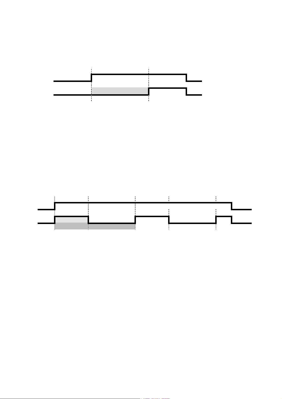
7.1 Off-Delay Mode

The following picture shows the timed response of the 'Off-delay' timer mode.

Picture 7-2: Off-delay Timer Mode Diagram

Input1

Output time duration

When 'Input1' of the timer is True, 'Output' is set True and the elapsed time counter is set to zero. When 'Input1' is False for longer than the 'time duration', 'Output' is set False.

That means it is specified the time duration that must elapse before the False output value is applied.

'Input2' of the timer is not used in this mode.

HAS55E03IM11S(1) [NGA-e (TFID Software 3.7.x)] CM PLC Page 10

Programmable Logic Control (PLC) on Control Module Level

7.2 On-Delay Mode

The following picture shows the timed response of the 'On-delay' timer mode.

Picture 7-3: On-delay Timer Mode Diagram

Input1

Output time duration

When 'Input1' of the timer is False, 'Output' is set False and the elapsed time counter is set to zero. When 'Input1' is True for longer than the 'time duration', 'Output' is set True.

That means it is specified the time duration that must elapse before the True output value is applied.

'Input2' of the timer is not used in this mode.

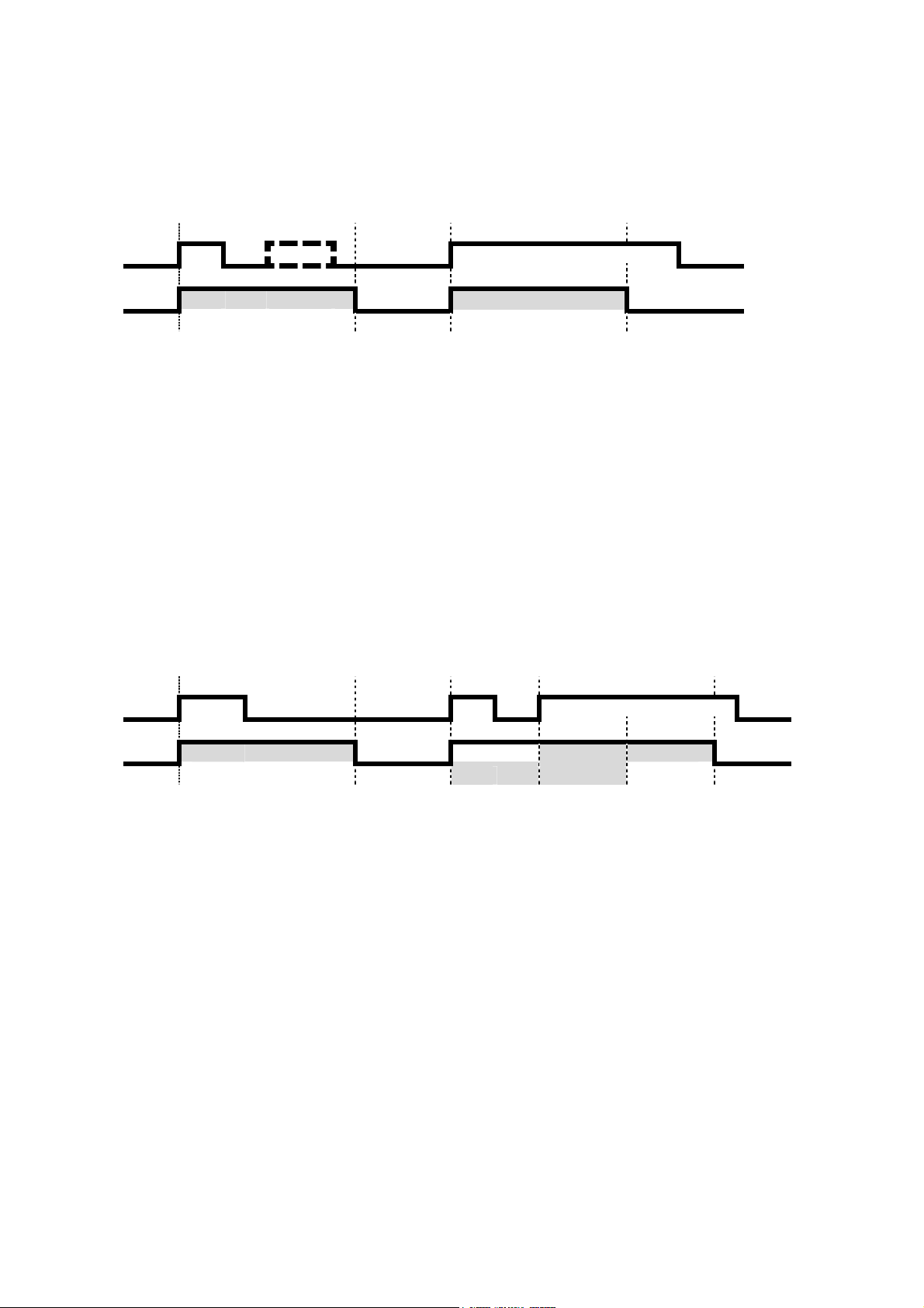
7.3 Repeated Pulse Mode

The following picture shows the timed behavior of the 'Repeated-Pulse' timer mode.

Picture 7-4: Repeated-Pulse Timer Mode Diagram

Input1

Output high duration period time

When 'Input1' of the timer is False, 'Output' is set False. When 'Input1' is True, the 'Output' is set according a square wave. On the rising edge of 'Input1' it begins with setting the 'Output' True until the high duration time is elapsed. Then 'Output' is set False and remains False for the rest of the period time. Then 'Output' is set True again for the high duration time, and so forth. This procedure goes on endless until Input1 is set False.

'Input2' of the timer is not used in this mode.

HAS55E03IM11S(1) [NGA-e (TFID Software 3.7.x)] CM PLC Page 11

Programmable Logic Control (PLC) on Control Module Level

7.4 Single Pulse Mode

The following picture shows the timed behavior of the 'Single Pulse' timer mode.

Picture 7-5: Single Pulse Timer Mode Diagram

Input1

Output time duration time duration

When 'Input1' of the timer changes from False to True (rising edge trigger) during 'Output' is False, 'Output' is set True until time duration is elapsed. Then 'Output' is set False.

'Input2' of the timer is not used in this mode.

Tips: The pulse width on Input1 is not relevant, the duration of the pulse on 'Output' is always the same. The level changes on Input1

are scanned on a configurable rate. Therefore the time between edges (rising and falling) has to be at minimum of this set update rate.

7.5 Retriggering Single Pulse Mode

The following picture shows the timed behavior of the 'Retriggering Single Pulse' timer mode.

Picture 7-6: Retriggering Single Pulse Timer Mode Diagram

retrigger

Input1

Output time duration time duration 2 time duration 1

When 'Input1' of the timer changes from False to True (rising edge trigger), 'Output' is set True until time duration is elapsed. Then 'Output' is set False. When 'Input1' changes from False to True again during Output is still set True the elapsing of the duration starts new.

'Input2' of the timer is not used in this mode.

Tips: The pulse width on Input1 is not relevant, the duration of the pulse on 'Output' is only stretched if there is a rising edge on Input1

again. The level changes on Input1 are scanned on a configurable rate. Therefore the time between edges (rising and falling) has to be at minimum of this set update rate.

HAS55E03IM11S(1) [NGA-e (TFID Software 3.7.x)] CM PLC Page 12

Programmable Logic Control (PLC) on Control Module Level

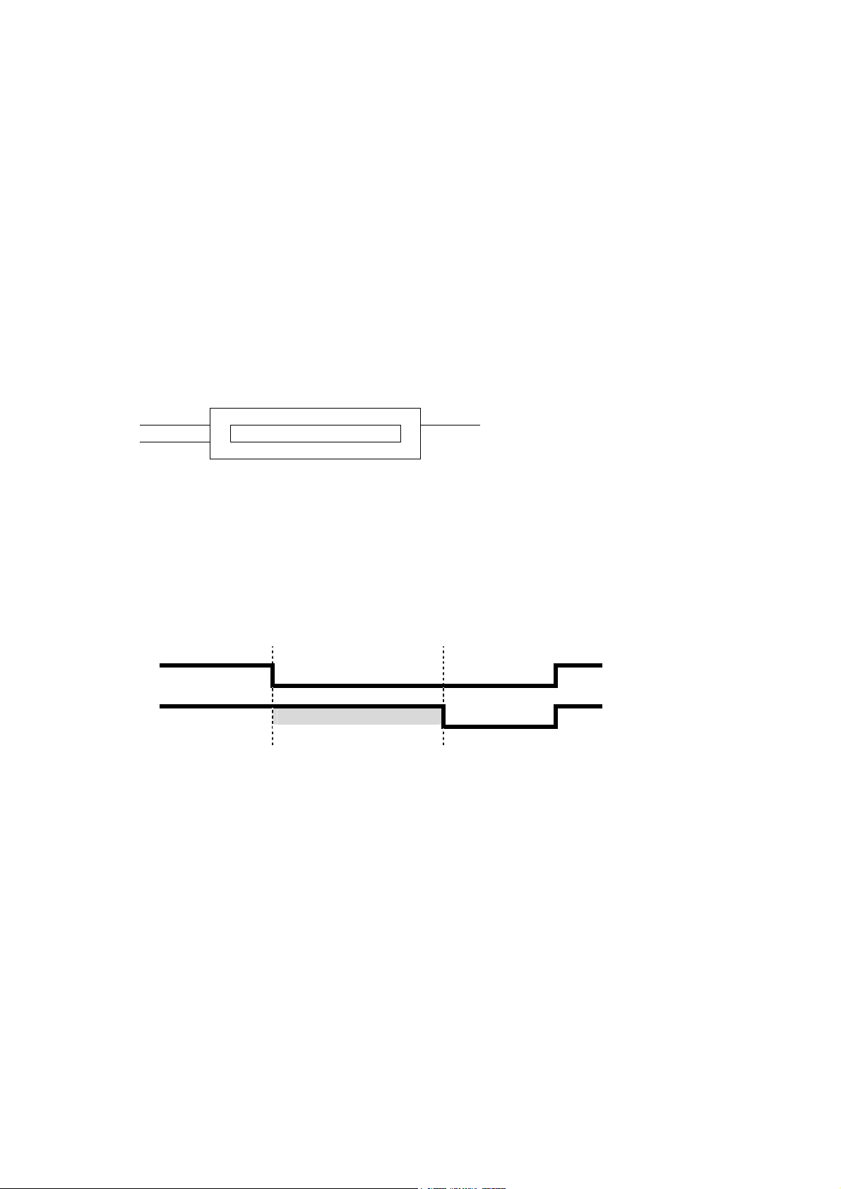
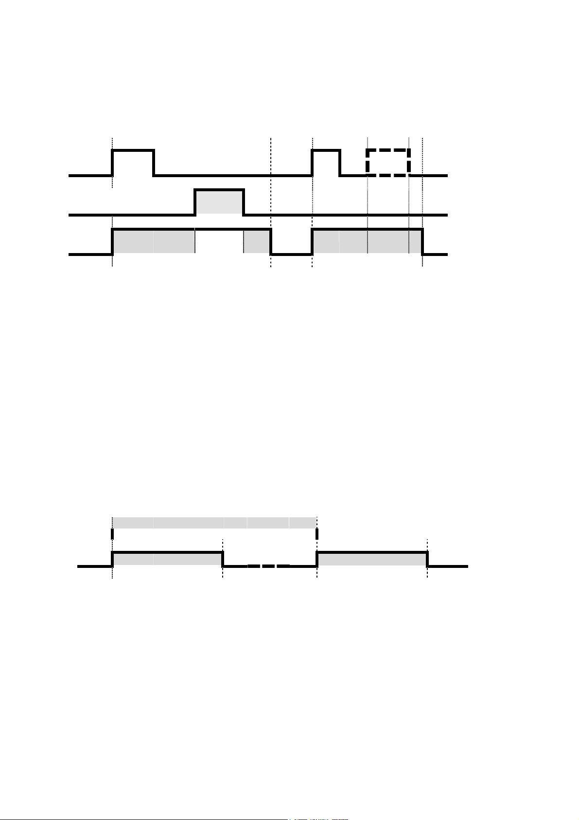
7.6 Inhibited Single Pulse Mode

The following picture shows the timed behavior of the 'Inhibited Single Pulse' timer mode.

Picture 7-7: Inhibited Single Pulse Timer Mode Diagram

Input1 (Trigger)

Input2 (Inhibit)

Output

When 'Input1' (logical trigger) of the timer transitions from False to True (rising edge trigger), 'Output' is set True until time duration is elapsed. Then 'Output' is set False.

'When 'Input2' (logical inhibit) of the timer is set during 'Output' is True (elapsing duration) the time stops and retains its value until Input2 transitions to False again. I.e., the duration time is increased by the inhibit pulses duration.

Tips: The duration of the pulse on 'Output' does not depend on the pulse width of Input1.

Inhibit

pulse

time duration time duration

The level changes on Input1 are scanned on a configurable rate. Therefore the time between edges (rising and falling) has to be at minimum of this set update rate.

7.7 Clock Triggered Pulse Mode

In the clock triggered pulse mode the behavior of the output is similar as in 'single pulse mode'. But the pulse is not triggered by Input1 but at a certain date/time.

Picture 7-8: Clock Triggered Pulse Timer Mode Diagram

interval time

Date Time Date Time

Output time duration time duration

When the real time clock of the device reaches a set date/time (time trigger), 'Output' is set True until time duration is elapsed. Then 'Output' is set False. This procedure recurs after a set interval time.

'Input1' and 'Input2' of the timer are not used in this mode.

HAS55E03IM11S(1) [NGA-e (TFID Software 3.7.x)] CM PLC Page 13

Programmable Logic Control (PLC) on Control Module Level

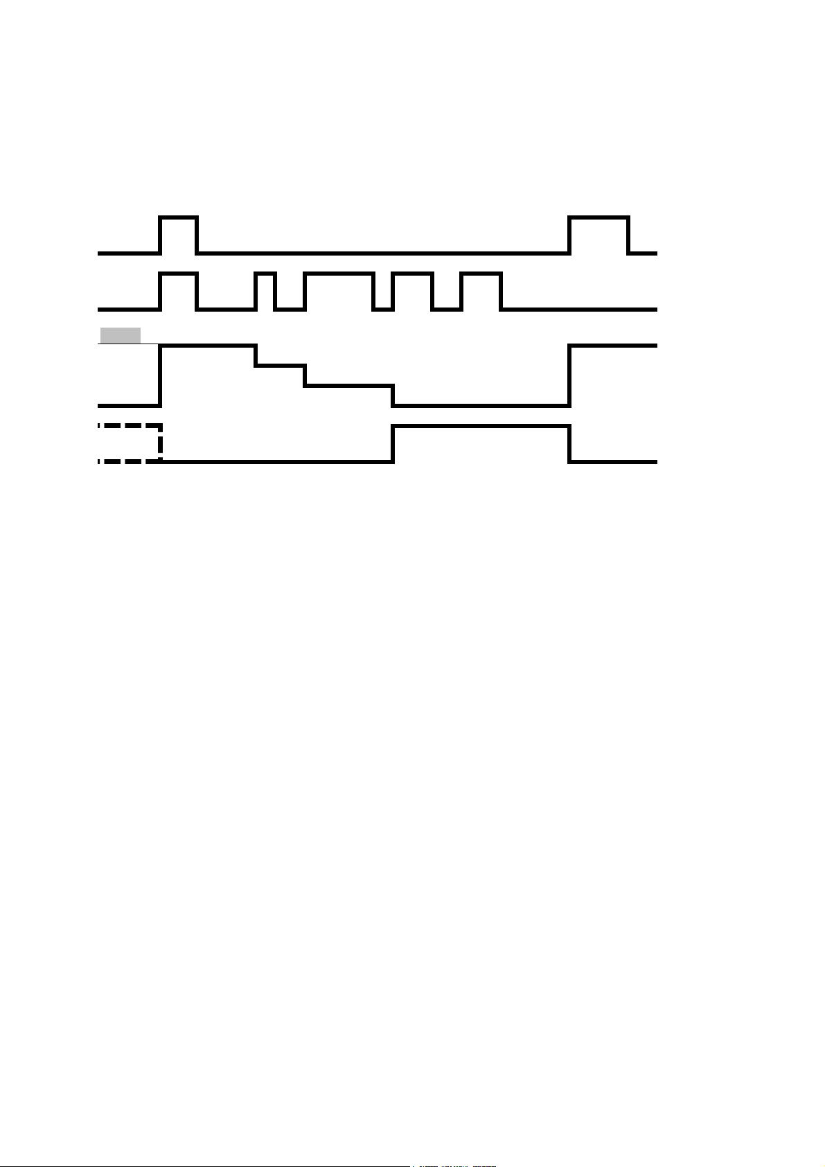
7.8 Counter Mode

The following picture shows the timed behavior of the 'Counter' mode.

Picture 7-9: Counter Mode Diagram

Input2 (Reset)

Input1 (Trigger)

Preset (here : 3) 2 internal 1 count 0

Output

When 'Input2' (logical 'Reset') of the timer is set to True, 'Output' is set False and the internal decrement counter is set to its preset value. After Input2 is set False the rising edges on Input1 (logical 'Trigger') decrement the counter. When the counter is less than or equal to zero, 'Output' is set True and the counter holds its value.

Tips: The level changes on Input1 are scanned on a configurable rate. Therefore the time between edges (rising and falling) has to be

at minimum of this set update rate.

HAS55E03IM11S(1) [NGA-e (TFID Software 3.7.x)] CM PLC Page 14

Programmable Logic Control (PLC) on Control Module Level

8 Menu Tree for the System PLC

The following pictures show the menu tree and the LON variables which are assigned to the single menu lines.

System configuration and diagnostics...

↓

System programmable logic control (PLC)...

↓

- System programmable logic control (PLC)-

Programming... Signals... Timer... Results...

PLC is: Cycle: 1.0 s

Program error in step: 0

Picture 8-1: System PLC Menu

With the 'PLC is' parameter we disable or enable PLC function. Also, with enabling the PLC there is the choice with which cyclic rate the programmed algorithm is called.

• Disabled

• has a Program Error (after trying to enable)

• Cycle 0.1 s

• Cycle 0.2 s

• Cycle 0.5 s

• Cycle 1.0 s

In the case of a program error by the 'Program error in step:' parameter is displayed in what step of the program this error happened. If there is no error this parameter equals '0'.

fct: PLCPROG_

PLCSTATUS

PLCERRLINE

HAS55E03IM11S(1) [NGA-e (TFID Software 3.7.x)] CM PLC Page 15

Programmable Logic Control (PLC) on Control Module Level

8.1 Submenu 'Signals'

All programmable signal assignments are done in the submenu 'Signals...".

System configuration and diagnostics...

↓

System programmable logic control (PLC)...

↓

Signals...

↓

- Signals -

Actions...

- Input signals -

Signal number: 65 Choose signal source module... Choose signal...

Signal name: Failure Signal comes from: MLT/CH1 Current signal level: Off

View... Outputs

Picture 8-2 : Input Signal Assignment of System PLC

The single signals of the pool (selected by 'Signal number') are assigned by first selecting the source analyzer module (AM) resp. analyzer channel of the requested signal and then the signal name itself. Please, note that it is only possible to modify the programmable type of signal numbers.

For the signal name's selection there is used an already implemented feature of the AMs. It has being used for the digital outputs of the DIO resp. the SIO module. It is the STCONT/STNAME variable mechanism. This mechanism provides the possibility to have a link to the LON variables of an AM which are listed in the STCONT enum. In the STNAME variable are listed the related human readable strings.

If we want to assign the signals not via the menu but via LON variable access we have to do the following steps:

1. Enter signal number by setting PLCSIGNUMC.

2. Enter the source of the signal by setting PLCSRCC to the TAG-variable's string of the requested channel.

3. Set PLC_ENTRYSIG (instead of using PLCSIGC) to the enum value that the signal has in the STCONTvariable.

PLCSIGNUMC [65 .. 128] PLCSRCSEL_ PLCSIGSEL_

PLCSIGC PLCSRCC PLCLEVELC

fct3: PLCSIGLST_ fct5: PLCOUTLST_

HAS55E03IM11S(1) [NGA-e (TFID Software 3.7.x)] CM PLC Page 16

Programmable Logic Control (PLC) on Control Module Level

8.1.1 Input Signals Listing

Via the View function key it is possible to show a listing of the whole input signal pool with the entered programmable as well as the fixed assignments.

The name of the fix signal assignments can be listed easily by using the enum variable PLC1INAME/ PLC2INAME which contains all the fix assigned signal's name (currently 64 names).

Here is shown a display according "Table 4-1: Example of an Input Signals Pool".

-- Signal List --

List offset: 60 Signal (o+1): ????: fix: Off Signal (o+2): ????: fix: Off Signal (o+3): ????: fix: Off Signal (o+4): ????: fix: Off Signal (o+5): Failure: MLT/CH1: Off Signal (o+6): Conc.Low-Low: MLT/CH1: Off Signal (o+7): Flow Low: MLT/CH3: On Signal (o+8): Cal. in progress: FID: Off Signal (o+9): Maintenance request: CLD: Off Signal (o+10): ????: ????: Off

<< Back... >>

Picture 8-3: Listing of Input Signal Assignment

LISTOFFSET MENU1LINE (live) MENU2LINE (live) MENU3LINE (live) MENU4LINE (live) MENU5LINE (live) MENU6LINE (live) MENU7LINE (live) MENU8LINE (live) MENU9LINE (live) MENU10LINE (live)

fct3: BACKVARS fct4: ESCAPE fct5: LOADVARS

HAS55E03IM11S(1) [NGA-e (TFID Software 3.7.x)] CM PLC Page 17

Programmable Logic Control (PLC) on Control Module Level

8.1.2 Output Signals Listing

Via the Outputs function key it is possible to show a listing of the whole output signal pool.

The name of the this fix output signal assignments can be listed easily by using the enum variable PLC1ONAME/PLC2ONAME which contains all the fix assigned signal's name.

Here is shown a display with Output Signals

-- Signal List --

List offset: 30 Signal (o+1): PLC Timer-1 In1: Off Signal (o+2): PLC Timer-2 In1: Off Signal (o+3): PLC Timer-3 In1: Off Signal (o+4): PLC Timer-4 In1: Off Signal (o+5): PLC Timer-5 In1: Off Signal (o+6): PLC Timer-6 In1: Off Signal (o+7): PLC Timer-7 In1: Off Signal (o+8): PLC Timer-8 In1: Off Signal (o+9): Reserved: Off Signal (o+10): Reserved: Off

<< Back... >>

Picture 8-4: Listing of Output Signal Assignment

LISTOFFSET MENU1LINE (live) MENU2LINE (live) MENU3LINE (live) MENU4LINE (live) MENU5LINE (live) MENU6LINE (live) MENU7LINE (live) MENU8LINE (live) MENU9LINE (live) MENU10LINE (live)

fct3: BACKVARS fct4: ESCAPE fct5: LOADVARS

HAS55E03IM11S(1) [NGA-e (TFID Software 3.7.x)] CM PLC Page 18

Programmable Logic Control (PLC) on Control Module Level

8.2 Submenu 'Actions'

All programmable action assignments are done in the submenu 'Actions...".

System configuration and diagnostics...

↓

System programmable logic control (PLC)...

↓

Signals...

↓

Actions...

↓

- Actions -

Action number: 1

Choose module...

Choose function...

Function name: AM:Zero-Cal Action goes to: MLT/CH1

View...

Picture 8-5 : Actions Assignment of System PLC

The single actions of the pool (selected by 'Action number') are assigned by first selecting the source analyzer module (AM) resp. analyzer channel of the requested action and then the function name itself.

For the function name's selection there is used an already implemented feature. It has being used for the digital inputs of the DIO module. It is the STINAME and AM_INPUT/DI_MSGE variable mechanism. This mechanism provides the possibility to have a link to functions of an AM which are listed in the STINAME-enum of the platform or at the AM_INPUT-enum of the single modules.

If we want to assign the actions not via the menu but via LON variable access we have to do the following steps:

1. Enter action number by setting PLCACTNUMC.

2. Enter the source of the signal by setting PLCACTSRCC to the TAG-variable's string of the requested

channel.

3. Set PLC_ENTRYACT (instead of using PLCACTIONC) to the corresponding enum value. This value is

calculated by usage of STINAME of the platform and AM_INPUT of the selected module.

If you select an action which is listed in STINAME, the enum value is just the value of STINAME. If you select an action which is listed in AM_INPUT you have to add the enum value of AM_INPUT to the number of available enum values of STINAME.

PLCACTNUMC [1..20]

PLCASRCSEL_

PLCACTSEL_

PLCACTIONC PLCACTSRCC

fct3: PLCACTLST_

HAS55E03IM11S(1) [NGA-e (TFID Software 3.7.x)] CM PLC Page 19

Programmable Logic Control (PLC) on Control Module Level

8.2.1 Actions Listing

It is possible to show a listing of the whole actions pool with the entered assignments as well as the corresponding signal levels.

System configuration and diagnostics...

↓

System programmable logic control (PLC)...

↓

Signals...

↓

Actions...

↓

View...

↓

-- Action List --

List offset: 0 Signal (o+1): AM:Zero-Cal: MLT/CH1: Off Signal (o+2): HoldAnalogOutput: MLT/CH1: Off Signal (o+3): ExtStatus1: MLT/CH3: On Signal (o+4): External failure: MLT1/CH2: Off Signal (o+5): SYS:Zero-Cal: Control Module: Off Signal (o+6): SYS:Cancel-Cal: Control Module: Off Signal (o+7): ????:????:Off Signal (o+8): ????:????:Off Signal (o+9): ????:????:Off Signal (o+10): ????:????:Off

<< Back... >>

Picture 8-6: Listing of Actions Assignment

LISTOFFSET MENU1LINE (live) MENU2LINE (live) MENU3LINE (live) MENU4LINE (live) MENU5LINE (live) MENU6LINE (live) MENU7LINE (live) MENU8LINE (live) MENU9LINE (live) MENU10LINE (live)

fct3: BACKVARS fct4: ESCAPE fct5: LOADVARS

HAS55E03IM11S(1) [NGA-e (TFID Software 3.7.x)] CM PLC Page 20

Programmable Logic Control (PLC) on Control Module Level

8.3 Submenu 'Timers'

The setup of the timers is configured in the submenu 'Timers...".

System configuration and diagnostics...

↓

System programmable logic control (PLC)...

↓

Timers...

↓

- Timers -

Timer number: 1 Timer mode: Off-delay Duration: 30 sec Period / Counts: 180 sec

Hours (0..23): 15 Minutes: 10 Month: 3 Day: 21

View... States...

Picture 8-7: Timers Setup of System PLC

PLCTMRNUMC [1..8] PLCTMRMODC [see Table 8-1] PLCDURATC [1..3600] PLCTIMC [1..3600] / PLCUC

PLCHOURC PLCMINUTC PLCMONTHC PLCDAYC

fct3: PLCTMRLST_ fct4: PLCTMRSTAT_

(variable unit)

The single timers are configured by first selecting the timer number itself (currently 1...8).

Further configuration parameters depend on the mode the timer has to run in. Therefore the mode has to be elected as next.

In following table see the selectable timer modes and the related meaning of the rest of the parameters.

Table 8-1: Different Timer Modes and the Related Meaning of the other Parameters

Timer mode Off-

delay

Duration delay

time Period/ Counts Hours Minutes Month Day

For more information on the different timer modes see also chapter "7 Time controlled Logic".

HAS55E03IM11S(1) [NGA-e (TFID Software 3.7.x)] CM PLC Page 21

On-

delay delay

time

- - period time

- - - - - - date/time of

Repeated-

Pulse

True pulse

width

[seconds]

Single-Pulse Retrig-Single-

Pulse

True pulse

width

- - - Interval time

min. True

pulse width

Inhib-Single-

Pulse

min. True

pulse width

Clock-Trig-

Pulse

True pulse

width

[minutes]

the pulse

Counter

-

Preset

count value

-

Programmable Logic Control (PLC) on Control Module Level

It is possible to show a listing of the timers' configuration.

System configuration and diagnostics...

↓

System programmable logic control (PLC)...

↓

Timers...

↓

View...

↓

- Timer Setup -

Offset (o): 0

Mode / Duration of timer 1+o: On-delay / 20 s Period / Counts: --- Next Start time: ---Mode / Duration of timer 2+o: Clock-Trig-Pulse / 20 s Period / Counts: 1440 min Next start Time & Date: 10:30:00 January 31, 2002 Mode / Duration of timer 3+o: Repeated-Pulse / 2 s Period / Counts: 6 s Next Start time: ----

<< Back... >>

Picture 8-8: Listing of Timers' Configuration

It is possible to show the actual states of timers' inputs and outputs as well as the current counting to perform the different timing functions.

System configuration and diagnostics...

↓

System programmable logic control (PLC)...

↓

Timers...

↓

States...

↓

- Timer States -

Offset (o): 0

Timer 1+o (In1/In2/Out): On/Off/Off Count: 3 Timer 2+o (In1/In2/Out): Off/On/On Count: 7 Timer 3+o (In1/In2/Out): Off/Off/ Off Count: 3 Timer 4+o (In1/In2/Out): On/On/On Count: 0 Timer 5+o (In1/In2/Out): Off/Off/Off Count: 0 << Back... >>

Picture 8-9: Display of Timers' States

LISTOFFSET MENU1LINE MENU2LINE MENU3LINE MENU4LINE MENU5LINE MENU6LINE MENU7LINE MENU8LINE MENU9LINE MENU10LINE

fct3: BACKVARS fct4: ESCAPE fct5: LOADVARS

LISTOFFSET

MENU1LINE MENU2LINE MENU3LINE MENU4LINE MENU5LINE MENU6LINE MENU7LINE MENU8LINE MENU9LINE MENU10LINE

fct3: BACKVARS fct4: ESCAPE fct5: LOADVARS

HAS55E03IM11S(1) [NGA-e (TFID Software 3.7.x)] CM PLC Page 22

Programmable Logic Control (PLC) on Control Module Level

8.4 Submenu 'Programming'

After having done the setup of the signals and eventually necessary timers we can do the programming of PLC algorithm itself. It is done in the submenu 'Programming...".

System configuration and diagnostics...

↓

System programmable logic control (PLC)...

↓

Programming...

↓

-- Programming --

Program offset (o): 0 Step (o+1): -2 Step (o+2): 67 Step (o+3): -4 Step (o+4): -3 Step (o+5): 37 Step (o+6): -8 Step (o+7): 1 Step (o+8): -7 Step (o+9): 0 Step (o+10): 0

<< Back... >>

Picture 8-10: Programming the System PLC

If we want to assign the signals not by means of the menu but via LON variable access we have to be aware of following:

1. The PLC-programming as well as the programming for the system calculator happens indirectly via the edit variable-array ED_INTx. To differ what the programming is for there exists the LON variable PROGTYP. Setting PROGTYP = 0 means we want to program the system calculator. Setting PROGTYP = 1 means we want to program the system PLC.

2. By using the variable LISTOFFSET we determine what part of the whole programming list we want to program. For example, setting LISTOFFSET = 60, means by usage of ED_INT1...ED_INT10 we are able to modify the program steps 61...70.

LISTOFFSET ED_INT1 ED_INT2 ED_INT3 ED_INT4 ED_INT5 ED_INT6 ED_INT7 ED_INT8 ED_INT9 ED_INT0

fct3: BACKVARS fct4: ESCAPE fct5: LOADVARS

HAS55E03IM11S(1) [NGA-e (TFID Software 3.7.x)] CM PLC Page 23

Programmable Logic Control (PLC) on Control Module Level

8.5 Submenu 'Results'

The results of the PLC calculations can be observed in the submenu 'Results...".

System configuration and diagnostics...

↓

System programmable logic control (PLC)...

↓

Results...

↓

-- Results (1/2) --

PLC-Output-1: On PLC-Output-2: Off PLC-Output-3: Off PLC-Output-4: Off PLC-Output-5: Off PLC-Output-6: Off PLC-Output-7: Off PLC-Output-8: On PLC-Output-9: Off PLC-Output-10: Off

Back... More...

Picture 8-11: Display of the System PLC Results

System configuration and diagnostics...

↓

System programmable logic control (PLC)...

↓

Results...

↓

More...

↓

-- Results (2/2) --

PLC-Output-11: On PLC-Output-12: Off PLC-Output-13: Off PLC-Output-14: Off PLC-Output-15: Off

Back... More...

PLCRESULT1 PLCRESULT2 PLCRESULT3 PLCRESULT4 PLCRESULT5 PLCRESULT6 PLCRESULT7 PLCRESULT8 PLCRESULT9 PLCRESULT10

fct4: ESCAPE fct5: PLCRESULTS2

PLCRESULT11 PLCRESULT12 PLCRESULT13 PLCRESULT14 PLCRESULT15

HAS55E03IM11S(1) [NGA-e (TFID Software 3.7.x)] CM PLC Page 24

Programmable Logic Control (PLC) on Control Module Level

9 Applications

9.1 Stream Control with an active System Calibration

If the system calibration is in the 'sample gas state' we do not want to have only one sample gas stream flowing but alternating 3 gas streams.

To realize this, we could use 2 timers which give us 3 different signal combinations. These 3 signal combinations are evaluated in that way that for each combination one of the streams is switched on.

Timer1-Out Timer2-Out Stream 1 Stream 2 Stream 3 On On On Off Off

Off On Off On Off Off Off Off Off On

Sample gas

Timer1-Out

Timer2-Out

Stream 1

Stream 2

Stream 3

To vary the switching durations we only have to configure the both timers.

Samplegas Valve = Sys-Valve1

-

For the program we presuppose following assignments:

HAS55E03IM11S(1) [NGA-e (TFID Software 3.7.x)] CM PLC Page 25

Timer 2

Off-Delay

Duration = 60 sec

-

Samplegas

&

Timer 1

Repeated-Pulse

In

Duration = 60 sec

Period = 180 sec

Out

In

Timer1-Out Timer2-Out

-

&

Out

&

Programmable Logic Control (PLC) on Control Module Level Input-ID 65 = Control Module: Sys.-Valve1 PLC-Result 1 = Stream 1 PLC-Result 2 = Stream 2 PLC-Result 3 = Stream 3

Step (1) -9 LOAD Step (2) 65 Control-Module SYS:Valve-1 (= Input-Signal 65) Step (3) -5 STORE to Step (4) 31 Timer1-Input1 (= Output-Signal 31) Step (5) -9 LOAD Step (6) 31 Timer1-Output (= Input-Signal 31) Step (7) -5 STORE to Step (8) 32 Timer2-Input1 (= Output-Signal 32) Step (9) -1 Step (10) -1 Step (11) -9 LOAD Step (12) 65 Control-Module SYS:Valve-1 (= Input-Signal 65) Step (13) -3 AND Step (14) 31 Timer1-Output Step (15) 32 Timer2-Output Step (16) -5 STORE to Step (17) 1 PLC-Result1 (= Output-Signal 1) => Stream 1 Step (18) -1 Step (19) -1 Step (20) -9 LOAD Step (21) 31 Timer1-Output Step (22) -4 INVERT Step (23) -3 AND Step (24) 65 Control-Module SYS:Valve-1 Step (25) 32 Timer2-Output Step (26) -5 STORE to Step (27) 2 PLC-Result2 (= Output-Signal 2) => Stream 2 Step (28) -1 Step (29) -1 Step (30) -9 LOAD Step (31) 31 Timer1-Output Step (32) -2 OR Step (33) 32 Timer2-Output Step (34) -4 INVERT (build: not Timer1-Output and not Timer2-Output) Step (35) -3 AND Step (36) 65 Control-Module SYS:Valve-1 Step (37) -5 STORE to Step (38) 3 PLC-Result3 (= Output-Signal 3) => Stream 3 Step (39) -7 End of program

HAS55E03IM11S(1) [NGA-e (TFID Software 3.7.x)] CM PLC Page 26

Programmable Logic Control (PLC) on Control Module Level

9.2 Remote Valve Switching with an active System Calibration

We have a MLT AM involved in a system calibration. But the MLT AM is not located nearby the platform device but in a certain distance.

Here we have the possibility to give the MLT AM2 valve switching commands via the LON network correspondingly to the activated system valves of the system calibration utility. These commanded valve states can be put onto the digital outputs of a local DIO board resp. onto the relays of a local SIO board.

We presuppose the following situation:

For the local DIO board of MLT-AM2 we do the following setup:

For the inputs signal pool of the System PLC we do following assignment:

For the action pool of the System PLC we do following assignment:

The System PLC program could look like as follows:

HAS55E03IM11S(1) [NGA-e (TFID Software 3.7.x)] CM PLC Page 27

MLT Analyzer

local AM1

System calibration

AM1-Ch1 MLT-AM2/CH1 MLT-AM2/CH2

Module setup Samplegas-Valve Valve-1 Valve-1 Valve-1

Zerogas-Valve Valve-2 Valve-2 Valve-2 Spangas1-Valve Valve-3 Valve-3 Valve-4 Spangas2-Valve Valve-3 Valve-3 Valve-4 Spangas3-Valve Valve-3 Valve-3 Valve-4 Spangas4-Valve Valve-3 Valve-3 Valve-4

setup of local DIO on AM2

Signal code

SignalDescription

Output #1 155 External Signal #1 of Ch1 Output #2 156 External Signal #2 of Ch1 Output #3 157 External Signal #3 of Ch1 Output #4 158 External Signal #4 of Ch1

Signal

Assignment

ID 71 Control Module: SYS:Valve-1

72 Control Module: SYS:Valve-2 73 Control Module: SYS:Valve-3 74 Control Module: SYS:Valve-4

Signal

Assignment

ID

1 MLT-AM2/CH1: ExtStatus1 2 MLT-AM2/CH1: ExtStatus2 3 MLT-AM2/CH1: ExtStatus3 4 MLT-AM2/CH1: ExtStatus4

remote located

MLT AM2

Ch1 & Ch2

local DIO

Programmable Logic Control (PLC) on Control Module Level

Step (1) -9 LOAD Step (2) 71 Control-Module SYS:Valve-1 (= Input-Signal 71) Step (3) -11 CALL action Step (4) 1 ExtStatus1 of MLT-AM2/CH1 (= Action #1) Step (5) -9 LOAD Step (6) 72 Control-Module SYS:Valve-2 (= Input-Signal 72) Step (7) -11 CALL action Step (8) 2 ExtStatus2 of MLT-AM2/CH1 (= Action #2) Step (9) -9 LOAD Step (10) 73 Control-Module SYS:Valve-3 (= Input-Signal 73) Step (11) -11 CALL action Step (12) 3 ExtStatus3 of MLT-AM2/CH1 (= Action #3) Step (13) -9 LOAD Step (14) 74 Control-Module SYS:Valve-4 (= Input-Signal 74) Step (15) -11 CALL action Step (16) 4 ExtStatus4 of MLT-AM2/CH1 (= Action #4) Step (39) -7 End of program

HAS55E03IM11S(1) [NGA-e (TFID Software 3.7.x)] CM PLC Page 28

NGA 2000

Software Manual

NGA 2000 System Calibration

Supplement: System Calibration

NGA Software Version 3.7.X

HAS55E03IM11S (1) [NGA-e (TFID Software 3.7.x)] 11/03 System Calibration Supplement - 1

NGA 2000 System Calibration

Beside the possibility to zero and span each TFID (CLD/FID) analyzer or analyzer module (MLT/CAT 200 channel) individually and independently from the others, System Calibration (SYSCAL) allows to combine the calibration procedures of ALL Analyzer Modules (AM’s) of an NGA 2000 analyzer system into a common process.

This is been achieved with a new assignment of the valves. The idea is not longer to require for each gas of each analyzer an own valve. Instead of we have a pool of valves. The valves of this pool can be assigned to the different gases of the analyzers. That also means different analyzers can share the same valve for their gases. So we have the possibility to reduce the number of valves and also the consumption of calibration gases.

The program, which will allow this, runs on the Control Module (CM) level and needs programmable Input/Output Modules (I/O’s: DIO and SIO) on control module level too (CM [system] I/O’s located in a platform or MLT, CAT 200 or TFID analyzer):

SIO: Standard I/O module with 2 to 8 analog outputs, RS 232/485 and 3 relay contacts

DIO: Digital I/O board with 8 digital inputs and 24 digital outputs

System calibration allows to use those outputs - relay contacts or digital outputs - to run calibration valves after assigning the valves to certain outputs (of course: physical connections between I/O’s and valves are required as well!). The assignment has to be done in a proper way which is described in the next chapters.

The displayed menus are also inscribed with the appropriate LON Variables.

HAS55E03IM11S (1) [NGA-e (TFID Software 3.7.x)] 11/03 System Calibration Supplement - 3

NGA 2000 System Calibration

2 Valves for system calibration

Before using the system calibration we have to put together the required valve pool. There are three types of I/O modules supporting this:

• DIO - 24 digital outputs / 8 digital inputs (max. 4 modules per CM)

• SIO - 3 digital outputs [relay contacts] (max. 1 module per CM)

• [CVU - 4 digital outputs (max. 4 modules per CM) – in progress; not available, c.f.]

Software supports up to 32 system valves.

2.1 Assigning an output port to a system valve

Assigning of an output can be accomplished by using the menus for selected output module (DIO, SIO or CVU [c.f.]). There we have to select the NGA Control Module as the Source Module. Control module then provides the signals for system valve V1...V32.

For example the DIO:

Analyzer and I/O module expert configuration...

↓

I/O module controls...

↓

DIO module(s)...

↓

- DIO-MODULE OUTPUTS-

Inputs... Outputnumber: 1 Choose module... Choose signal... Invert output: DISABLED Module status: NORMAL Slot ID: 1 Signal name: SYS:VALVE-1 Signal level: OFF Signal comes from: NGA Control Module

• select "Outputnumber"

• then choose ”NGA Control Module“ as module

• then choose the wanted valve “SYS: VALVE-x“ as signal

DIOOUTNUMC

DIOOUTINVC DIOMODSTAC DIOSLOTIDC DIOOUTSIGC DIOOUTSTATC DIOOUTSRCC

There we have to

Supplement - 4 System Calibration HAS55E03IM11S (1) [NGA-e (TFID Software 3.7.x)] 11/03

NGA 2000 System Calibration

It is also possible to configure the DIO outputs via LON Variables (i.e. SLTA adapter or protocol).

Therefore is the LON variable "DIOOUT_ENTRYSIG" which corresponds to “DIOOUTSIGC“ and evaluates enum values of “ST1NAME” (enum values 0..19), “ST2NAME” (enum values

20..39) or “ST3NAME” (enum values 40..59).

For digital output we have to set-up variables in following order.

1. DIOSLOTIDC

2. DIOOUTNUMC

3. DIOOUTSRCC

4. DIOOUT_ENTRYSIG SYS: VALVE-1 = 20 (enum value in ST2NAME)

SYS: VALVE-2 = 21 . . . . . . SYS:VALVE-32 = 51 (enum value in ST3NAME)

For each needed system valve we have to repeat these appropriate selections.

It is also possible to distribute the system valves onto different output modules.

HAS55E03IM11S (1) [NGA-e (TFID Software 3.7.x)] 11/03 System Calibration Supplement - 5

NGA 2000 System Calibration

3 Operating System Calibration

Because there are many possibilities how to use SYSCAL it must be customized through the Expert Operator. There we can find the menu “System Calibration“ from were we can do the required set-ups and start routines.

System configuration and diagnostics...

↓

System calibration...

↓

System Calibration

Calibration/Test procedures...

Calibration Sequence Programming... Times for interval operation... Set-up analyzer modules...

Meaning of displayed menu points:

• Calibration/Test procedures...: starting and stopping of system calibration and test

procedures

• Calibr. Sequ. Programming...: programming of user defined calibration sequences

• Times for interval operation...: setting up of automatically started system

calibrations

• Set-up analyzer modules...: include and set-up different analyzer modules into

system calibration.

Supplement - 6 System Calibration HAS55E03IM11S (1) [NGA-e (TFID Software 3.7.x)] 11/03

NGA 2000 System Calibration

3.1 Set-up analyzer modules

Before we can run any system calibration features we have to include the different analyzer modules (AM’s) into system calibration by set-up needed parameters. Only after correct setting up, an AM is included into system calibration and only then it makes sense to go into the other menus.

System configuration and diagnostics...

↓

System calibration...

↓

Set-up analyzer modules...

↓

Analyzer Set up

Choose analyzer module....

Gas type: SPANGAS-1 Assigned to system valve: V5 Purge time: 20 s

Note: Ranges are always calibrated separately !

_______________________________________________

Analyzer module: MLT/CH2 Module enabled for system-cal: NO

View...

SCAMGAS SCVALVE SCPURGE

SCMODULE SCCONTROL

Setting up an AM for system calibration means assigning valves from system valve pool.

The Control Module provides support of up to 32 system-valves V1....V32. We have to

decide which valves deliver which gases for an analyzer module. Also we have to know the purge time from a valve to the AM.

For each of the following types in the parameter „Gas type“ we have to assign a valve and the appropriate purge time :

• SAMPLE-GAS

• ZERO-GAS

• SPANGAS-1 (span gas for range 1)

• SPANGAS-2 (span gas for range 2)

• SPANGAS-3 (span gas for range 3)

• SPANGAS-4 (span gas for range 4)

Optionally we can assign a blowback valve but this is not mandatory.

Conditions for the assignment:

• Once a valve has been assigned to be a sample gas valve for any AM it must not

be used for zero or span gases !

• The zero valve of an AM can not be a span valve of the same AM.

• All upper gas types have to be assigned to a system-valve.

• If we assign a blowback valve it must not be used for any other gases.

HAS55E03IM11S (1) [NGA-e (TFID Software 3.7.x)] 11/03 System Calibration Supplement - 7

NGA 2000 System Calibration

Example for an analyzer system:

V 7 V1 AM1 AM2 AM3

V2 AM4

V 8 V3 AM5

V 4 V5 V6

Blowback gas Calibration gas mixtures

Appropriate assignment:

AM1 AM2 AM3 AM4 AM5 SAMPLE-GAS V1 V1 V1 V2 V3 ZERO-GAS V4 V4 V5 V5 V6 SPANGAS-1 V5 V5 V4 V6 V5 SPANGAS-2 V5 V5 V4 V6 V5 SPANGAS-3 V6 V5 V4 V4 V4 SPANGAS-4 V6 V5 V4 V4 V4 BLOWBACK V7 V7 V7 - V8

As we can see, additionally we can assign blowback valves in the "Gas Type" set-up. In the upper example these are valves V7 and V8. The blowback valve is switched on then during a blowback procedure, all other valves are switched off. The blowback procedure looks for the purge times which are configured for this blowback valves. For the procedure is taken then the maximal purge time of the assigned blowback valves.

This entire assigning procedure is to perform for all analyzer modules which should be included in system calibration. To display the assigned valves and purge times for each AM we can push the soft key „View...“.

If we want to exclude an AM from SYSCAL we can do this by entering an invalid valve. We can watch in the display whether an AM is enabled for system calibration.

Attention: Remember to assign a system valve to an output port!

Supplement - 8 System Calibration HAS55E03IM11S (1) [NGA-e (TFID Software 3.7.x)] 11/03

NGA 2000 System Calibration

3.2 Programming Calibration Sequences

Beside the standard programs “zero calibration“ and “zero/span calibration“ it is possible to run the system calibration in an user definable order of up to 40 steps.

The menu to set-up this feature looks as follows.

System configuration and diagnostics...

↓

System calibration...

↓

Calibration sequence programming...

↓

-- Calibration Sequence Programming --

Step #: 1 Calibration procedure type: ZERO-CAL Choose specific analyzer module... Select all analyzer modules! Program steps 1-10... Program steps 11-20... Program steps 21-30... Program steps 31-40...

_______________________________________________ Analyzer-module: MLT/CH3

SCSTEP SCCALTYPE1

SCSTEPMOD

For programming the sequence you must

1. select “Step #“

2. select “Calibration procedure type“

3. select module

Repeat this order for all program steps.

The programmable “Calibration procedure types“ are:

1. NoOp no operation (for deleting a step in an existing program)

2. Zero-Cal do a zero calibration

3. Span-Cal do a span-calibration for all available ranges

4. Zero/Span-Cal do a zero-cal then a span-cal for all available ranges

5. Span1-Cal do a span calibration only for range #1

6. Span2-Cal do a span calibration only for range #2

7. Span3-Cal do a span calibration only for range #3

8. Span4-Cal do a span calibration only for range #4

9. END-OF-PGRM end of sequence

10.Blowback do a blowback

HAS55E03IM11S (1) [NGA-e (TFID Software 3.7.x)] 11/03 System Calibration Supplement - 9

NGA 2000 System Calibration

For each step we have the choice to select a specific AM or to activate the step for all enabled AM’s.

After the program is input, the appropriate menu can give an overview of the current program:

-- Calibration Sequence Program --

Step #1: Zero-Cal:ALL Step #2: Span-Cal: FID Step #3: Span-Cal: CLD Step #4: Span1-Cal:MLT/CH1 Step #5: Span2-Cal:MLT/CH1 Step #6: Span3-Cal:MLT/CH1 Step #7: Span4-Cal:MLT/CH1 Step #8: Span3-Cal:MLT/CH2 Step #9: END-OF-PROGRAM Step #10: END-OF-PROGRAM

Supplement - 10 System Calibration HAS55E03IM11S (1) [NGA-e (TFID Software 3.7.x)] 11/03

NGA 2000 System Calibration

3.3 Set-up general parameters

One general parameter is "Calibration Procedures in Test-Mode". It is located in the menu "Calibration/Test procedures".

System configuration and diagnostics...

↓

System calibration...

↓

Calibration/Test procedures...

↓

-- Calibration/Test Procedures --

Start Zeroing all ranges! Start Zeroing and Spanning all ranges ! Start calibration program ! Cancel calibration! Calibration Procedures in Test-Mode: No Test Procedures...

Calibration type: ZERO-CAL Program step: 1 Calibration time: 16 s Previous calibration time: 57 s

Blowback Result...

SCTESTMOD

SCCALTYPE2 SCPROGSTEP SCCALTIME1 SCCALTIME2

With this parameter we can run all the calibration procedures either in the defined mode or in a test mode. The test mode means that the valve switching and waiting for purge times is done in the same manner like in the normal calibration procedure. The only difference is that the single calibrations of the modules and the appropriate times the modules would need for the calibration are not done.

HAS55E03IM11S (1) [NGA-e (TFID Software 3.7.x)] 11/03 System Calibration Supplement - 11

NGA 2000 System Calibration

A further general parameter is "Timeout for Gastest". It is located in the menu "Test procedures".

System configuration and diagnostics...

↓

System calibration...

↓

Calibration/Test Procedures...

↓

Test procedures...

↓

-- Test Procedures --

Gastest of specific module SAMPLE-Gas Timeout for Gastest (0 = no timeout) 180 s Choose specific analyzer module...

_______________________________________________ Procedure time: 10 s Analyzer-module: MLT/CH3

SCTESTGAS SCTIMEOUT

SCCALTIME1 SCSTEPMOD

This parameter is related to the possibility to activate a gas valve of a specific module for test purposes. Here we can determine a time after which an activated gas test automatically switches back onto SAMPLE-Gas. Is this parameter set to "0" no automatic back switching is done.

Supplement - 12 System Calibration HAS55E03IM11S (1) [NGA-e (TFID Software 3.7.x)] 11/03

NGA 2000 System Calibration

3.4 Controlling System Calibration

After setting-up there is the possibility to start 3 different modes:

system zero-calibration: In this mode a zero-cal of all modules, which are enabled

for SYSCAL, will be performed. The order of modules depends on purge time for zero-valves because the whole calibration is time optimized.

system zero/span-calibration: In this mode will be performed a zero-cal and a span-cal

for every enabled AM. The order of calibration is optimized to have a minimum of calibration time. The only condition is to have for each AM first the zero-cal and after this the span-cal. With zero-cal an AM is zeroed with all ranges together, the span-cal is done separately for all available ranges. A range is available if its span-gas value is > 0.0.

user defined sequence program: In this mode the user is responsible for the optimization.

See set-up of this mode.

blowback procedure: In this mode are switched off the assigned sample gas

and calibration gas valves. An assigned blowback valve is switched on.

gas test: It is also possible to switch for test purposes onto a

specific gas of a specific module. A calibration is not done.

Any mode can be started by the following instances:

• Manually by operator interaction

• Triggered by programmable input (DIO)

• protocol command

• Programmed time-automatic (no gas test possible!)

• LON Variable “CMFUNC »

It is also possible to cancel a running system calibration. This can be done by the following instances:

• Manually by operator interaction

• Triggered by programmable input (DIO)

• protocol command

• LON Variable “CMFUNC”

There is no priority by which way SYSCAL can be started. If SYSCAL was started it can not be restarted by a further instance. Only after canceling it can be restarted.

HAS55E03IM11S (1) [NGA-e (TFID Software 3.7.x)] 11/03 System Calibration Supplement - 13

NGA 2000 System Calibration

3.4.1 Control via menu system

The possibility to control via menu is located in the menu page „Calibration/Test procedures“. There can be started and stopped any kind of system calibration respectively test procedure.

System configuration and diagnostics...

↓

System Calibration...

↓

Calibration/Test procedures...

↓

Calibration/Test Procedures

Start Zeroing all ranges! Start Zeroing and Spanning all ranges ! Start calibration program ! Cancel calibration! Calibration Procedures in Test-Mode: No Test Procedures...

Calibration type: ZERO-CAL Program step: 1 Calibration time: 16 s Previous calibration time: 57 s

Blowback Result...

SCTESTMOD

SCCALTYPE2 SCPROGSTEP SCCALTIME1 SCCALTIME2

During a running SYSCAL there can be watched current information:

• running calibration type

• running program step of user defined program (other modes than user program show a

„0“!)

• consumed calibration time

• calibration time of last valid SYSCAL

Supplement - 14 System Calibration HAS55E03IM11S (1) [NGA-e (TFID Software 3.7.x)] 11/03

NGA 2000 System Calibration

The result of calibration for included AM’s is displayed in an own menu page. This can be achieved by soft key “Result...“ from different menu pages of SYSCAL.

- Calibration Results -

Choose analyzer module... Analyzer-module: CLD Enabled for system-cal: No

_______________________________________________ Result of last run: OK Successfully calibrated ranges: 1+2+4 Zero-Cal fail of any analyzer module: NO Span-Cal fail of any analyzer module: YES

SCMODULE SCCONTROL

SCLRESULT SCVALIDITY SCRESULT1 SCRESULT2

Remember to run the calibration procedures as a test without actually to calibrate assert parameter "Calibration Procedures in Test-Mode" to <Yes>.

It is also possible to switch for test purposes onto a specific gas of a specific module. This possibility is located in menu "Test procedures".

System configuration and diagnostics...

↓

System Calibration...

↓

Calibration/Test Procedures...

↓

Test procedures...

↓

-- Test Procedures --

Gastest of specific module SAMPLE-Gas Timeout for Gastest (0 = no timeout) 180 s Choose specific analyzer module...

_______________________________________________ Procedure time: 10 s Analyzer-module: MLT/CH3

SCTESTGAS SCTIMEOUT

SCCALTIME1 SCSTEPMOD

HAS55E03IM11S (1) [NGA-e (TFID Software 3.7.x)] 11/03 System Calibration Supplement - 15

NGA 2000 System Calibration

Here we first choose the specific analyzer module and then we select at the parameter "Gastest of specific module" the required gas.

Each of the following types is possible:

• All closed

• Zero-Gas

• SAMPLE-Gas (test mode deactivated)

• SpanGas-1 (span gas for range 1)

• SpanGas-2 (span gas for range 2)

• SpanGas-3 (span gas for range 3)

• SpanGas-4 (span gas for range 4)

• Blowback

With parameter "Timeout for Gastest" we can determine a time after which the activated gas test switches automatically back onto SAMPLE-Gas.

Is this parameter set to "0" the automatic back switching is not done automatically and user must break this mode with a "Cancel Calibration" Command.

Supplement - 16 System Calibration HAS55E03IM11S (1) [NGA-e (TFID Software 3.7.x)] 11/03

NGA 2000 System Calibration

3.4.2 Control System Calibration by LON Variables

SYSCAL can also be controlled by LON Variable CMFUNC. Setting this variable will cause the appropriate function (see following table).

CMFUNC function which is started

1 system zero-calibration 2 system zero/span-calibration 3 user defined sequence program 4 cancel a running system calibration 5 blowback procedure

We can also realize some other functionality with setting of LON Variables. Therefore see the appropriate menu pages, where the concerned variables are documented.

For example: "Test procedures".

--Test Procedures --

Gastest of specific module SAMPLE-Gas Timeout for Gastest (0 = no timeout) 180 s Choose specific analyzer module...

_______________________________________________

Procedure time: 10 s Analyzer-module: MLT/CH3

SCTESTGAS SCTIMEOUT

SCCALTIME1 SCSTEPMOD

Here we have first to set variable SCSTEPMOD similar to the TAG of the requested analyzer module. Setting SCTIMEOUT will set the timeout. And setting variable SCTESTGAS to the appropriate enum value will start the procedure.

Table of enum values and procedures:

SCTESTGASfunction enum value

???? Zero-

Gas

SAMPLEGas

Span Gas-1

Span Gas-2

Span Gas-3

Span Gas-4

Blowback

0 1 2 3 4 5 6 7

HAS55E03IM11S (1) [NGA-e (TFID Software 3.7.x)] 11/03 System Calibration Supplement - 17

NGA 2000 System Calibration

3.4.3 Control System Calibration by Programmable Input

We can use the possibility to control SYSCAL by triggering with a programmable input. This feature is supported by inputs of the DIO Module. Assigning of an programmable input can be accomplished by using the menus for DIO module.

Analyzer and I/O-module expert configuration...

↓

I/O module controls...

↓

DIO module(s)...

↓

Inputs...

↓

-- DIO- Module Inputs --

Inputnumber: 5 Choose module... Choose function...

_______________________________________________ Slot ID: 1 Signal name: SYS:Cancel-Cal Signal level: OFF Signal comes from: Control Module

DIOINPNUMC

DIOSLOTIDC DIOINPSIGC DIOINPSTATC DIOINPSRCC

There we have to select

1. wanted input number

2. the appropriate module as Source Module (see following table)

3. the wanted function for system calibration

The provided functions for system calibration are:

function source

module SYS:Zero-Cal CM start system zero-calibration - 6 SYS:Zero/Span-Cal CM start system zero/span-calibration - 7 SYS:Program-Cal CM start user defined sequence program

SYS:Cancel-Cal CM stop a running procedure and disable

SYS:CAL-Test-Mode CM switches into test mode switches off test mode 10 SYS:AM-Zero-Gas AM switches zero gas-valve stop a running procedure 11 SYS:AM-Span-Gas1 AM switches span gas-valve for range 1 stop a running procedure 12 SYS:AM-Span-Gas2 AM switches span gas-valve for range 2 stop a running procedure 13 SYS:AM-Span-Gas3 AM switches span gas-valve for range 3 stop a running procedure 14 SYS:AM-Span-Gas4 AM switches span gas-valve for range 4 stop a running procedure 15 SYS:Blowbackl CM start system blowback procedure - 22

function (positive edge)

calibration

any start commands

function (negative edge)

- 8

enable starting commands 9

enum value in STINAME

Please take notice that all actions are edge-triggered. Therefore take care of functionality of

positive as well as negative edge.

Supplement - 18 System Calibration HAS55E03IM11S (1) [NGA-e (TFID Software 3.7.x)] 11/03

NGA 2000 System Calibration

It is also possible to configure the DIO inputs only per LON Variables (i.e. SLTA-adapter or protocol). Therefore is the LON variable "DIOINP_ENTRYSIG" which corresponds to “DIOINPSIGC” and evaluates enum values of “STINAME”.

For each digital input we have to set-up variables in following order.

1. DIOSLOTIDC

2. DIOINPNUMC

3. DIOINPSRCC

4. DIOINP_ENTRYSIG (see enum value in STINAME)

HAS55E03IM11S (1) [NGA-e (TFID Software 3.7.x)] 11/03 System Calibration Supplement - 19

NGA 2000 System Calibration

3.4.4 Control System Calibration by protocol command

We can start and stop SYSCAL over serial interface by protocol commands. Therefore the commands SCAL, STBY and ASTZ has to be used.

Start-Command: SCAL Kx m (n)

m (type of SYSCAL)

0 = ZERO-CAL K0 n = 1: switch into test mode 1 = ZERO/SPAN-CAL K0 2 = PROGRAM K0 else: switch into normal mode 3 = TEST ZERO-GAS K1...999 timeout in sec 4 = TEST SPAN-GAS1 K1...999 timeout in sec 5 = TEST SPAN-GAS2 K1...999 timeout in sec 6 = TEST SPAN-GAS3 K1...999 timeout in sec 7 = TEST SPAN-GAS4 K1...999 timeout in sec 8 = TEST CLOSE GASES K1...999 timeout in sec 9 = BLOWBACK K0 not used

Kx (channel number)

n (optional parameter)

If optional parameter n is not in command string the appropriate variable is not changed.

Starting condition: All attached AM’s are in the Standby-Mode (AK STBY) and the variable CALSTAT is 0, otherwise the response is BUSY (BS).

Stop-Command: STBY K0

Only using K0 will stop running SYSCAL-procedure (besides all the procedures of the other AM’s).

Check-Command: ASTZ K0

The ASTZ K0 command gives the information if a SYSCAL-procedure is running or not. If running it returns a “SCAL” if not this string is missed.

Supplement - 20 System Calibration HAS55E03IM11S (1) [NGA-e (TFID Software 3.7.x)] 11/03

NGA 2000 System Calibration

3.4.5 Time controlled System Calibration

To activate a time controlled system calibration we have to set-up this in own menu pages. For each of the time controlled procedures exists an own menu page.

System configuration and diagnostics...

System Calibration...

Times for interval operation...

-- Times for Zero Interval Operation --

Zero-Cal is: ENABLED Start time Month: 2 Day: 20 Hours: 10 Minutes: 15 Interval time: 24 h Next calibration events...

Time & Date: 15:26:10 February 19, 2001

ZeroSpan Program Blowbac

System configuration and diagnostics...

System Calibration...

Times for interval operation...

-- Times for Zero&Span Interval Operation --

Zero&Span Cal is: DISABLED Start time Month: 2 Day: 20 Hours: 10 Minutes: 15 Interval time: 24 h Next calibration events...

Time & Date: 15:26:10 February 19, 2001

↓

fct2: ZeroSpan

↓

k

SCSTZERO

SCBGNZERO1 SCBGNZERO2 SCBGNZERO3 SCBGNZERO4 SCIVZERO

S_TIME

SCSTZEROSPAN

SCBGNZSPAN1 SCBGNZSPAN2 SCBGNZSPAN3 SCBGNZSPAN4 SCIVZEROSPAN

S_TIME

HAS55E03IM11S (1) [NGA-e (TFID Software 3.7.x)] 11/03 System Calibration Supplement - 21

NGA 2000 System Calibration

System configuration and diagnostics...

↓

System Calibration...

↓

Times for interval operation...

↓

fct3: Program

↓

-- Times for Program Cal Interval Operation --

Program Cal is: DISABLED Start time Month: 2 Day: 20 Hours: 10 Minutes: 15 Interval time: 24 h Next calibration events...

Time & Date: 15:26:10 February 19, 2001

System configuration and diagnostics...

↓

System Calibration...

↓

Times for interval operation...

↓

fct5: Blowback

↓

-- Times for Blowback Interval Operation --

Blowback is: DISABLED Start time Month: 2 Day: 20 Hours: 10 Minutes: 15 Interval time: 24 h Next calibration events...

Time & Date: 15:26:10 February 19, 2001

SCSTPRGM

SCBGNPRGM1 SCBGNPRGM2 SCBGNPRGM3 SCBGNPRGM4 SCIVPRGM

S_TIME

SCSTBLOWB

SCBGNBLOWB1 SCBGNBLOWB2 SCBGNBLOWB3 SCBGNBLOWB4 SCIVBLOWB

S_TIME

Supplement - 22 System Calibration HAS55E03IM11S (1) [NGA-e (TFID Software 3.7.x)] 11/03

NGA 2000 System Calibration

For the different SYSCAL-modes there is the possibility to

• enable/disable the time controlled activation

• determine start time of activities (date/time of current year)

• determine in which time intervals after start time the activation is done

Attention: Other than in some AM-functionalities the interval time is to be input as interval hours. For example, for a weekly calibration you have to calculate 24 h * 7 = 168 h.

Is the input date/time before present point of date/time then there are added further interval times until it is later.

We can display the calculated times in menu page „next calibration events“... But these times will only appear when the appropriate time controlled procedure type is enabled.

System configuration and diagnostics...

↓

System Calibration...

↓

Times for interval operation...

↓

Next calibration events...

↓

Next Calibration Events

Zero-Cal: 10:15:00 February 22, 2003

Zero&Span-Cal: 10:15:00 February 22, 2003

Program-Cal: 10:15:00 February 22, 2003

Blowback: 10:15:00 February 22, 2003

Time & Date: 15:26:10 February 19, 2003

Menu1Line

Menu2Line

Menu3Line

Menu4Line

S_TIME

HAS55E03IM11S (1) [NGA-e (TFID Software 3.7.x)] 11/03 System Calibration Supplement - 23

NGA 2000 System Calibration

3.5 Calibrate single Analyzers

Each specific analyzer has still the possibility to start a calibration over other instances than SYSCAL. For this functionality we now have some additional considerations.

• Do not start a calibration of a single AM during a running SYSCAL. This will confuse the

valve switching and the calibration commands of SYSCAL. Therefore look also for all automatic start instances of an analyzer.

• A single calibration cannot use the purge times of system valve settings. Instead of we

have to set-up the AM’s own parameters in the manner to wait for the required purge time after a valve switching.

• It is refused to start single calibration of a second AM if the needed calibration gas valve is

also any calibration gas valve of the first started AM.

These considerations are valid for all AM’s which are included into SYSCAL.

Supplement - 24 System Calibration HAS55E03IM11S (1) [NGA-e (TFID Software 3.7.x)] 11/03

NGA 2000 System Calibration

4 Functionality

4.1 Gas flow

The gas flow through the analyzers can be configured in any way:

1. only serial

2. only parallel

3. serial and parallel mixed

Sample 1 V1 AM1 AM2 AM3

Sample 2 V2 AM4

Sample 3 V3 AM5

V 4 V 5 V 6

Calibration gas mixtures

Connections for program logic and flow configurations:

• To each AM (MLT/ CAT 200 channel) must be assigned a sample gas valve.

• During a calibration of an AM the assigned sample gas valve will be closed and returns to

the OPEN-state after the calibration of the AM is done.

• The calibration gases can only flow into an AM if sample gas valve is closed.

• With a opened sample gas valve it is expected to actually flow sample gas.

The state of assigned sample gas valve also decides about some AM specific states!

HAS55E03IM11S (1) [NGA-e (TFID Software 3.7.x)] 11/03 System Calibration Supplement - 25

NGA 2000 System Calibration

4.2 Running system calibration

The system calibration is running in an own task. This task is only allowed to run once. Any try to restart this task is refused.

The main steps SYSCAL task has to do are realized in the following way.

1. Fill all actions to do into a sequence buffer.

2. Make some preparations before starting the actions

3. Work through the sequence buffer

4. Restore states and make some other finishing work

The contents of the sequence buffer depends on the type of SYSCAL (ZERO_ALL, ZEROSPAN_ALL or USER_PROG). With the start command this type is delivered.

It is allowed to cancel the SYSCAL task. This is realized by setting a parameter to a defined value. This parameter is watched during step 3("working through the sequence buffer"). If a cancel is caused the task cancels its current action in step 3, works through step 4 and ends.

Canceling the SYSCAL task per digital input will also disable any further starting action as long as the digital input will stay at “cancel state“.

Supplement - 26 System Calibration HAS55E03IM11S (1) [NGA-e (TFID Software 3.7.x)] 11/03

NGA 2000 System Calibration

4.2.1 Filling sequence buffer

The contents of the sequence buffer depends on

• calibration types and belonging module type

• coherence of modules and system valves

An evaluation procedure has the choice of listed action types.

Calibration types module type NOP ALL-AM’s USER-STEP Nr ZERO-CAL single AM SWITCH_VALVE mask SPAN-CAL Evaluation- PURGEWAIT time ZERO/SPAN-CAL procedure ZERO AM SPAN1-CAL SPAN AM range SPAN2-CAL CALWAIT AM SPAN3-CAL SPAN4-CAL END-OF-PGRM

action types action data

One calibration type has following sequence frame:

1. SWITCH_VALVE

2. do different PURGEWAIT, ZERO, or SPAN which are possible with this valve adjustment

(order is determined by shortest purge time)

3. do different CALWAIT (wait for finishing a started calibration)

The evaluation procedure optimizes the order of actions by time. The only condition is in case of ZERO/SPAN-CAL, where an AM has to do first its "ZERO" before any of its "SPAN’s" can be done.

The PURGEWAIT-delay-measurement is started with the last SWITCH_VALVE-action.

We can see, that the SYSCAL-types "ZERO_ALL" and "ZEROSPAN_ALL" are special cases of a user program.

• ZERO_ALL: ZERO CAL of ALL AM’s

• ZEROSPAN_ALL: ZERO/SPAN CAL of ALL AM’s

HAS55E03IM11S (1) [NGA-e (TFID Software 3.7.x)] 11/03 System Calibration Supplement - 27

NGA 2000 System Calibration

Example of a filled sequence buffer

Assignment of modules, system valves and purge times:

AM1 AM2 AM3 SAMPLE-GAS V1 / 5 sec V1 / 5 sec V2 / 4sec ZERO-GAS V4 / 10 sec V4 / 10 sec V5 / 12 sec SPANGAS-1 V5 / 10 sec V5 / 10 sec V6 / 12 sec SPANGAS-2 V5 / 10 sec V5 / 10 sec V6 / 12 sec SPANGAS-3 V6 / 10 sec V5 / 10 sec V4 / 14 sec SPANGAS-4 V6 / 10 sec V5 / 10 sec V4 / 14 sec

To do is following user program:

1. ZERO-CAL ALL modules

2. SPAN4-CAL AM2

3. END-OF-PGRM

Belonging sequence buffer:

action type action data[0] action data[1] USER_STEP 1 SWITCH_VALVE 0006 hex (V4, V2) PURGEWAIT 10 ZERO AM1 PURGEWAIT 10 ZERO AM2 CALWAIT AM1 CALWAIT AM2 SWITCH_VALVE 0011 hex (V5,V1) PURGEWAIT 12 ZERO AM3 CALWAIT AM3 USER_STEP 2 SWITCH_VALVE 0012 hex (V5, V2) PURGEWAIT 10 SPAN AM2 4 CALWAIT AM2 END-OF-PGRM

The size of sequence buffer is currently 320.

Supplement - 28 System Calibration HAS55E03IM11S (1) [NGA-e (TFID Software 3.7.x)] 11/03

NGA 2000 System Calibration

4.2.2 Before starting actions

Before any action of sequence buffer is done there are some preparations to do:

• store previous calibration time for the case of canceling

• previous calibration time is now the actual one

• actual calibration time is reset

• cancel any running calibration of an AM

4.2.3 Control of actions

4.2.3.1 Switch valves

The SWITCH_VALVE action just takes the action data[0] (valve mask) for the new setting of system valves. We have just to modify LON variable STCONT3, STCONT4 and partially STCONT5 , which are linked to system valves.

This action also resets time (takes system tick) for delay measurement of purge times.

4.2.3.2 Wait for Purging

The PURGEWAIT action looks for the present time went over since last SWITCH_VALVE action.

For the still required difference up to the needed purge time is now waited. It gives time to other tasks. If there is no additional time to wait it is continued directly with next action.

HAS55E03IM11S (1) [NGA-e (TFID Software 3.7.x)] 11/03 System Calibration Supplement - 29

NGA 2000 System Calibration

4.2.3.3 Zero Calibration

Before starting of zero calibration there are some parameters (LON variables) to modify. After ending system calibration these modified variables are restored to their previous value.

• CONTROL: This variable determines which instance is controlling range of an

AM. The parameter is set to "controlled by control module"

• ZERORNGS: This variable determines if all ranges are zeroed together or

separately. The parameter is set to "zero all ranges together".

• AMSERPHYSTAT: This variable exists only in a multi-channel AM (MLT!) and

determines if the AM has a serial/parallel gas flow.

The parameter is set to "parallel gas flow" because only this state allows SYSCAL to calibrate the different channels simultaneously.

After modifying these parameters zero calibration is started by LON variable:

• AMFN: This variable can start functions on a AM. It is set to the value for

function "Zero".

4.2.3.4 Span Calibration

The span calibration can be done only in single ranges. Any action for a span calibration in a range can only be done if "span gas value <> 0.0".

Before starting then span calibration there are some parameters (LON variables) to modify. After ending system calibration these modified variables are restored to their previous value.

• CONTROL: This variable determines which instance is controlling range of an

AM. The parameter is set to "controlled by control module"

• CALRANGES: This variable determines if all ranges are spanned together or

separately. The parameter is set to "span all ranges separately".

• AMSERPHYSTAT: This variable exists only in a multi-channel AM (MLT!) and

determines if the AM has a serial/parallel gas flow.

The parameter is set to "parallel gas flow" because only this state

allows SYSCAL to calibrate the different channels simultaneously.

• CRANGE: This variable controls the current range of an AM. It is set to the

respectively required range.

After modifying these parameters span calibration is started by LON variable:

• AMFN: This variable can start functions on a AM. It is set to the value for

function "Span".

Supplement - 30 System Calibration HAS55E03IM11S (1) [NGA-e (TFID Software 3.7.x)] 11/03

NGA 2000 System Calibration

4.2.3.5 Wait for Finishing Calibration

Any AM has the LON variables

• CALSTAT

Whether the selected AM is still calibrating or not, is checked by reading the variable CALSTAT.

This CALSTAT-check is done in time intervals. During the intervals time is given to other tasks.

4.2.4 Finishing System Calibration

After system calibration was working through the sequence buffer or it was canceled there is to do some finishing work.

• Actualize some displayed LON variables

• Look for some still running calibrations in case of canceling and cancel them, too.

• Restore modified LON variables of AM’s.

• Switch system valves to sample gas state for all AM’s

• Cause to set any AM’s LON variable PROCESS = "valid sample gas" after purging time of

sample gas valve.

HAS55E03IM11S (1) [NGA-e (TFID Software 3.7.x)] 11/03 System Calibration Supplement - 31

NGA 2000 System Calibration

4.3 Running Single Analyzer Calibration

A single analyzer calibration also needs to switch appropriate system valves.

The difference to the system calibration is that calibration procedure of AM is already running and we have to respond upon this state.

The reaction is possible by watching any change of the LON variable CALSTAT.

• CALSTAT_ZERO (zero calibration in progress): switch off belonging sample valve and

switch on zero valve.

• CALSTAT_SPAN (span calibration in progress): switch off belonging sample valve and

switch on span valve appropriate to current state of CRANGEvariable.

• CALSTAT_DONE (calibration finished): switch on sample valve and switch off calibration gas valves.

After a calibration command the AM itself is responsible to wait the required purge times until calibration actually is done.

The reaction onto a CALSTAT-change is only active if no system calibration is running.

Supplement - 32 System Calibration HAS55E03IM11S (1) [NGA-e (TFID Software 3.7.x)] 11/03

NGA 2000 System Calibration

4.4 Holding analog outputs of the SIO and avoid limit violation alarms

Any AM has LON variable:

• PROCESS

This variable is an input-variable. Its meaning is to tell the AM that another instance is not allowing the measurement sample to flow valid.

In the AM are some states depending from PROCESS.

• "valid measurement" only if PROCESS = "valid sample gas".

• holding analog outputs if PROCESS = "no valid sample gas"

• watching limit violations is switched off if PROCESS = "no valid sample gas"

It's now the task of the system calibration to handle the variable PROCESS for any involved AM. This is done in the following way:

Any switching of a system valve looks if in the switched valves is a sample valve of any AM. If yes, then it sets PROCESS like follows.

sample gas valve

time delay PROCESS-

variable

switched off - sample not valid switched on purge time of sample valve sample valid

It's very important to notice following:

SYSCAL only watches state of appropriate sample gas valve for setting of PROCESSvariable.

Any additional valve, serial to sample valve, which can switch off flow of sample gas cannot be registered for logic of PROCESS variable.

HAS55E03IM11S (1) [NGA-e (TFID Software 3.7.x)] 11/03 System Calibration Supplement - 33

NGA 2000 System Calibration

Supplement - 34 System Calibration HAS55E03IM11S (1) [NGA-e (TFID Software 3.7.x)] 11/03

Additional AK Commands

Additional AK Protocol Commands

NGA 2000

NGA Software Version 3.7.x

HAS55E03IM11S(1) [NGA-e (TFID Software 3.7.x)] 04/03 AK Page 1

Additional AK Commands

SHDA Kn deactivate “Hold” Status

Description: We have the possibility to activate the "Hold" feature not only per calibration. We can do this

also by AK Command “SHDE”. With command “SHDA” we have the possibility to deactivate an activated "Hold" again.

Rosemount NGA 2000 TFID Hydrocarbon Analyzer Module SW 3.7 Supplement to SW 3.4 Software-1st Ed. Manuals & Guides

Specifications and Main Features

Frequently Asked Questions

User Manual

ESSENTIAL INSTRUCTIONS

Table of Contents

Addendum for Software Revision 3.6.x to 3.4.x

1. Display Controls Menu

2. Analyzer Basic Controls (calibration) & Setup Menu

3. Tolerances Menu

Calculator on Control Module Level

1.1 Principle of program set-up

1.2 Live values (real measuring values)

1.5 Menu tree for the system calculator

2 Display Calculator Results on Mini-bargraph

2.2 Assign signals and convenient names

3 Assignment to SIO Analog Outputs

Programmable Logic Control (PLC) on Control Module Level

Contents

2 Principle of Program Setup

7 Time controlled Logic

7.3 Repeated Pulse Mode

7.4 Single Pulse Mode

7.5 Retriggering Single Pulse Mode

7.6 Inhibited Single Pulse Mode

7.7 Clock Triggered Pulse Mode

7.8 Counter Mode

8 Menu Tree for the System PLC

9.1 Stream Control with an active System Calibration

9.2 Remote Valve Switching with an active System Calibration

Supplement: System Calibration

Table of Contents

4 Functionality

Additional AK Protocol Commands