Rosemount 54eC Conductivity/Resistivity Analyzer Manuals & Guides

Download

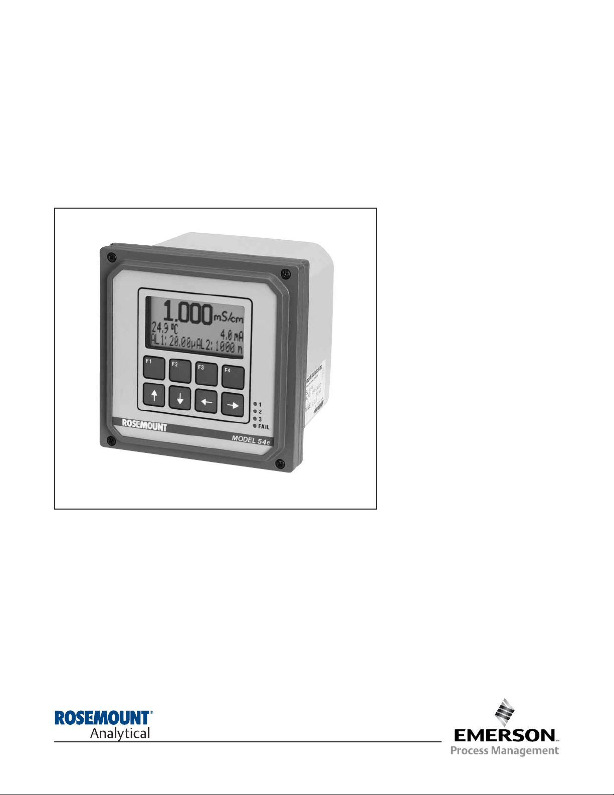
Model 54eC

Conductivity/Resistivity HART

Analyzer/Controller

Instruction Manual

51-54eC/rev.F May 2006

ESSENTIAL INSTRUCTIONS

READ THIS PAGE BEFORE PRO-

CEEDING!

Rosemount Analytical designs, manufactures, and tests its products to meet many national and international standards. Because these instruments are sophisticated technical products, you must properly install, use, and maintain them to ensure they continue to operate within their normal specifications. The following instructions must be adhered to and integrated into your safety program when installing, using, and maintaining Rosemount Analytical products. Failure to follow the proper instructions may cause any one of the following situations to occur: Loss of life; personal injury; property damage; damage to this instrument; and warranty invalidation.

• Read all instructions prior to installing, operating, and servicing the product. If this Instruction Manual is not the correct manual, telephone 1-800-654-7768 and the requested manual will be provided. Save this Instruction Manual for future reference.

• If you do not understand any of the instructions, contact your Rosemount representative for clarification.

• Follow all warnings, cautions, and instructions marked on and supplied with the product.

• Inform and educate your personnel in the proper installation, operation, and maintenance of the product.

• Install your equipment as specified in the Installation Instructions of the appropriate Instruction Manual and per applicable local and national codes. Connect all products to the proper electrical and pressure sources.

• To ensure proper performance, use qualified personnel to install, operate, update, program, and maintain the product.

• When replacement parts are required, ensure that qualified people use replacement parts specified by Rosemount. Unauthorized parts and procedures can affect the product’s performance and place the safe operation of your process at risk. Look alike substitutions may result in fire, electrical hazards, or improper operation.

• Ensure that all equipment doors are closed and protective covers are in place, except when maintenance is being performed by qualified persons, to prevent electrical shock and personal injury.

WARNING

ELECTRICAL SHOCK HAZARD

Making cable connections to and servicing this instrument require access to shock hazard level voltages which can cause death or serious injury, therefore, disconnect all hazardous voltage before accessing the electronics.

Relay contacts made to separate power sources must be disconnected before servicing.

Electrical installation must be in accordance with the National Electrical Code (ANSI/NFPA-

70) and/or any other applicable national or local codes.

Unused cable conduit entries must be securely sealed by non-flammable closures to provide enclosure integrity in compliance with personal safety and environmental protection requirements. Use NEMA 4X or IP65 conduit plugs supplied with the instrument to maintain the ingress protection rating (IP65).

For safety and proper performance this instrument must be connected to a properly grounded three-wire power source.

Proper relay use and configuration is the responsibility of the user. No external connection to the instrument of more than 60VDC or 43V peak allowed with the exception of power and relay terminals. Any violation will impair the safety protection provided.

Do not operate this instrument without front cover secured. Refer installation, operation and servicing to qualified personnel.

WARNING

This product is not intended for use in the residential, commercial or light industrial environment per

certification to EN50081-2.

Emerson Process Management

Liquid Division

2400 Barranca Parkway Irvine, CA 92606 USA Tel: (949) 757-8500 Fax: (949) 474-7250

http://www.raihome.com

About This Document

This manual contains instructions for installation and operation of the Model 54eC Conductivity/Resitivity HART Analyzer/Controller.

The following list provides notes concerning all revisions of this document.

Rev. Level

Date Notes

0 9/99 This is the initial release of the product manual. The manual

has been reformatted to reflect the Emerson documentation style and updated to reflect any changes in the product offering.

0 11/01 Added trim output info

A 12/01 Revised spec and temp slope info

B 6/02 updated drawings on page 8

C 2/03 Removed Figure 3-2 (sensor wiring photo)

D 4/03 Updated CE info

E 4/05 Added note re ordering circuit board stack on page 63.

F 5/06 Noted 0-20 mA limitation for HART versions on pp. 21, 26, & 32.

MODEL 54eC TABLE OF CONTENTS

MODEL 54eC

MICROPROCESSOR ANALYZER

TABLE OF CONTENTS

Section Title Page

1.0 DESCRIPTION AND SPECIFICATIONS ................................................................ 1

1.1 General Description................................................................................................. 1

1.2 Description of Controls ............................................................................................ 1

1.3 Specifications........................................................................................................... 2

1.4 Ordering Information................................................................................................ 4

2.0 INSTALLATION....................................................................................................... 5

2.1 Locating the Controller ............................................................................................ 5

2.2 Unpacking and Inspection ....................................................................................... 5

2.3 Mechanical Installation ............................................................................................ 5

3.0 WIRING ................................................................................................................... 7

3.1 General.................................................................................................................... 7

3.2 Power Input Wiring .................................................................................................. 7

3.3 Analog Output Wiring .............................................................................................. 7

3.4 Alarm Relay Output Wiring...................................................................................... 7

3.5 Sensor Wiring.......................................................................................................... 9

3.6 Final Electrical Check.............................................................................................. 9

4.0 CALIBRATION ........................................................................................................ 11

4.1 Initial SetUp ............................................................................................................. 12

4.2 Entering the Cell Constant ...................................................................................... 13

4.3 Zeroing the Controller.............................................................................................. 14

4.4 Selecting the Temperature Compensation Type ..................................................... 15

4.5 Temperature Calibration .......................................................................................... 16

4.6 Calibrating the Sensor............................................................................................. 17

4.7 Temperature Compensation Options....................................................................... 18

4.8 Hold Mode ............................................................................................................... 19

4.9 Output Trim.............................................................................................................. 19

5.0 SOFTWARE CONFIGURATION ............................................................................. 20

5.1 Changing Output Setpoints (PID only) .................................................................... 24

5.2 Changing Alarm Setpoints....................................................................................... 25

5.3 Changing Output Setpoints (Normal) ...................................................................... 26

5.4 Testing Outputs and Alarms .................................................................................... 27

5.5 Choosing Display Options ....................................................................................... 29

5.6 Changing Output Parameters.................................................................................. 31

5.7 Changing Alarm Parameters ................................................................................... 34

6.0 THEORY OF OPERATION ..................................................................................... 40

6.1 Conductivity ............................................................................................................. 40

6.2 Temperature Correction........................................................................................... 40

6.3 Interval Timer........................................................................................................... 41

6.4 Alarm Relays ........................................................................................................... 42

6.5 Time Proportional Control (TPC) Mode................................................................... 42

6.6 Normal Mode........................................................................................................... 43

6.7 Analog Outputs........................................................................................................ 43

6.8 Controller Mode Priority........................................................................................... 44

6.9 PID Control.............................................................................................................. 45

MODEL 54eC TABLE OF CONTENTS

TABLE OF CONTENTS (Continued)

Section Title Page

7.0 SPECIAL PROCEDURES AND FEATURES ......................................................... 49

7.1 Password Protection................................................................................................ 49

7.2 Configuring Security ................................................................................................ 50

7.3 Temperature Slope Procedure (Linear Compensation) ........................................... 51

7.4 Determining Unknown Temperature Slopes (Linear Compensation)...................... 52

7.5 Changing the Reference Temperature..................................................................... 53

7.6 Special Substance Calibration................................................................................. 54

8.0 TROUBLESHOOTING ........................................................................................... 55

8.1 Displaying Diagnostic Parameters........................................................................... 58

8.2 Troubleshooting Guidelines..................................................................................... 59

8.3 Replacement Parts .................................................................................................. 63

9.0 RETURN OF MATERIALS ..................................................................................... 64

LIST OF FIGURES

Figure No. Title Page

1-1 Main Display Screen............................................................................. 1

2-1 Wall Mounting....................................................................................... 5

2-2 Pipe Mounting....................................................................................... 6

2-3 Panel Mounting..................................................................................... 6

3-1 Power Input and Relay Output Wiring for Model 54eC......................... 8

3-2 Sensor Wiring Diagram ........................................................................ 10

5-1 Outline of Menu Levels......................................................................... 23

5-2 Interval Timer Examples....................................................................... 38

6-1 Time Proportional Control..................................................................... 42

6-2 The Process Reaction Curve................................................................ 47

LIST OF TABLES

Table No. Title Page

4-1 Typical Temperature Slopes ................................................................. 15

5-1 Conductivity Settings List ..................................................................... 20

6-1 Controller Mode Priority Chart .............................................................. 44

8-1 Diagnostic Messages ........................................................................... 56

8-2 Quick Troubleshooting Guide ............................................................... 57

8-3 Troubleshooting Guide ......................................................................... 60

MODEL 54eC SECTION 1.0

DESCRIPTION AND SPECIFICATIONS

SECTION 1.0

DESCRIPTION AND SPECIFICATIONS

1.1 GENERAL DESCRIPTION

The Model 54eC conductivity controller is a device used to measure conductivity in chemical processes. Conductivity is a function of ion concentration, ionic charge, and ion mobility. Ions in water conduct current when an electrical potential is applied across electrodes immersed in the solution. A controller system consists of a microprocessor-based controller, a conductivity probe, and mounting hardware.

The controller can use an electrodeless toroidal probe or a contacting probe with metal electrodes. Electrodeless (also called inductive) conductivity measurement is especially useful for solutions containing abrasive solids, highly conductive, or highly corrosive materials. The contacting probe is used where conductivity is below 200 micromhos, such as water rinses in metal finishing or ultrapure boiler water applications. It uses an electrode design for greater sensitivity because these water solutions tend to be non-fouling.

All adjustments to the current outputs, alarm relays, and calibration of the pH and temperature inputs can be made using the controller's membrane keypad.

1.2 DESCRIPTION OF CONTROLS

Figure 1-1 shows a diagram of the main display screen. Similar diagrams are used throughout this manual. The primary variable is continuously displayed in large numerals. The process temperature and primary current output value are always displayed on the second line of the main display screen. The third line can be configured to read several different items, as desired. In this case, it is displaying setpoints for alarms 1 and 2.

The F1-F4 keys are multifunction. The active operation for that key is displayed as a label just above each function key as needed. For example, F1 is usually labeled Exit and F4 may be labeled Edit, Save, or Enter. Pressing Enter 4 will access sub-menus, while pressing Edit allows changing values and Save stores the values in memory. Esc 3 can be used to abort unwanted changes. Exit 1 returns to the previous screen. Other labels may appear for more specialized tasks.

The up t and down b keys are used to:

1. Move the cursor (shown in reverse video) up and down on the menu screens.

2. Scroll through the list of options available for the field shown in reverse video. When the last item

of a menu has been reached, the cursor will rest on the third line of the display. If the cursor is on the second line, there are more items to see with the down arrow key.

3. Scroll through values when a highlighted numerical value is to be set or changed.

The right and left keys are used to move the cursor to the next digit of a number.

Green LEDs (labeled 1, 2, and 3) indicate when alarm relays 1, 2, and 3 are energized. The fourth relay indicates a fault condition. When a fault occurs, the red LED (labeled FAIL) lights up, a descriptive error message is displayed, and the action of the outputs and relays will be as described in Section 5.6 and Section 5.7 under fault value (e.g. 22 mA).

The red LED also indicates when the interval timer routine is activated and when the time limit has been reached on a feed limit timer. For more information on these subjects, see Section 5.7.

FIGURE 1-1. Main Display Screen

500

µS/cm

26.2°C. 12.0 mA AL1: 2000μS AL2: 500μS

MODEL 54eC SECTION 1.0

DESCRIPTION AND SPECIFICATIONS

1.3 SPECIFICATIONS

PHYSICAL SPECIFICATIONS - GENERAL

Enclosure: Epoxy-painted cast aluminum

NEMA 4X (IP65),144 X 144 X 132mm, DIN size (5.7 X 5.7 X 5.2 in.)

Front Panel: Membrane keyboard with tactile feed

back and user selectable security. Light gray, blue and white overlay. Light gray enclosure, dark gray bezel.

Display: Back-lit dot matrix LCD (7.0 x 3.5 cm), blue

on gray-green. The display contrast is compensated for ambient temperature.

Process Variable Character Height: 16mm (0.6 inch)

Electrical Classification:

Class I, Division 2, Groups A, B, C, & D. T5 Ta=50°C. Dust ignition proof: Class II, Division 1, Groups E, F, & G; Class III.

CSA-LR34186:

Max. relay contact rating: 28 Vdc; 110 Vac; 230 Vac; 6 amps resistive

FM: Max. relay contact rating: 28 Vdc resistive

150 mA - Groups A & B; 400 mA - Group C; 540 mA - Group D

Power:

Code -01: 100 - 127 VAC, 50/60 Hz ± 6%, 6.0 W;

200 - 253 VAC, 50/60 Hz ± 6%, 6.0 W

Code -02: 20 - 30 VDC, 6.0 W

Current Outputs:

Output 1: Process, Raw conductivity, or Temperature

Output 2: Process, Raw conductivity, or Temperature

Each output is galvanically isolated, 0-20 mA or 420 mA into 500 ohms maximum load at 115/230 Vac or 24 Vdc (Code -02) or 500 ohms maximum load at 100/200 Vac. Output 1 includes digital signal 4-20 mA superimposed HART (Code -09 only).

EMI/RFI :EN61326

LVD (Code -01 only) : EN61010-1

Ambient Temperature:

0 to 50°C (32 to 122°F)

NOTE: The analyzer is operable from

-20 to 60°C (-4 to

140°F) with some degradation in display performance.

Relative Humidity: 95%, non-condensing

Alarms:

Relay 1 - Process, Temperature, or Interval Timer

Relay 2 - Process, Temperature, or Interval Timer

Relay 3 - Process, Temperature, or Interval Timer

Relay 4 - Fault alarm

Each relay has a dedicated LED on the front panel.

Relay Contacts: Relays 1-3: Epoxy sealed form A

contacts, SPST, normally open.

Relay 4: Epoxy sealed form C, SPDT.

Resistive Inductive

28 Vdc 5.0 Amps 3.0 Amps

115 Vac 5.0 Amps 3.0 Amps

230 Vac 5.0 Amps 1.5 Amps

Weight/Shipping Weight: 1.1 kg/1.6 kg (2.5 lb/3.5 lb)

MODEL 54eC SECTION 1.0

DESCRIPTION AND SPECIFICATIONS

INSTRUMENT SPECIFICATIONS @ 25°C

Measurement Range: –15 to 200°C (5 to 392°F)

Contacting: 0-20,000 µS/cm Toroidal: 0-2 S/cm

Accuracy of Analyzer: (Analyzer connected to simulated sensor input)

Contacting Sensors: ±0.5% of reading, ± .005 µS/cm Inductive Sensors: ±1% of reading, 200 µS/cm to 2 S/cm, ± 5 µS/cm

Repeatability: ±0.25% of reading Stability: ±0.25% of output range/month, noncumulative Ambient Temperature Coefficient: ± 0.01% of reading/°C Temperature Compensation: -15 to 200°C (5 to 392°F) (automatic or manual) Temperature Correction: High purity water (dilute sodium chloride), cation conductivity (dilute hydrochloric

acid), linear temperature coefficient (0.0 to 5.00%/°C), or none. High purity water and cation conductivity temperature correction apply between 0 and 100°C. Linear temperature coefficient can be applied between

-5 and 200°C (23 to 392°F).

CONTACTING SENSORS

Conductivity Sensor 142, 400 142, 400 140, 141

Model Number 402, 403, 404 402, 403, 404 400, 402, 403

Cell Constant (/cm) 0.01 0.1 1.0

Recommended Conductivity 0-25 1-2000 10-10,000**

Range* (μS/cm)

INDUCTIVE SENSORS

Conductivity Sensor

Model Number 226 228 225 222 (1in.) 222 (2 in.) 242

Nominal Cell Constant 1.0 3.0 3.0 6.0 4.0 *

Minimum Conductivity (μS/cm) 50 200 200 500 500 100*

Maximum Conductivity (μS/cm) 1,000,000 2,000,000 2,000,000 2,000,000 2,000,000 1,500,000*

* Model 242 values depend on sensor configuration and wiring.

* For sensor linearity equal to or better than 1% with ENDURANCE series. ** ENDURANCE sensors with cell constant of 1.0/cm may be used for conductivity up to

20,000 μS/cm with linearity equal to or better than 2%.

SENSOR CHOICE GUIDELINES

The Model 54eC is compatible with both contacting and inductive conductivity sensors. The best sensor for an application depends on many factors, among them are the conductivity to be measured, the compatibility of the sensor's wetted materials with the process chemicals and conditions, and the mounting arrangement. The tables below are provided as an aid for choosing an appropriate sensor.

MODEL 54eC SECTION 1.0

DESCRIPTION AND SPECIFICATIONS

1.4 ORDERING INFORMATION

The Model 54eC Conductivity Microprocessor Analyzer is housed in a rugged, NEMA 4X (IP65) epoxy- painted cast aluminum enclosure and is compatible with both contacting and inductive conductivity sensors. Standard features include a back-lit dot-matrix liquid crystal display, sensor diagnostics, dual isolated outputs, and four relays. The analyzer can measure conductivity, resistivity, or percent (%) concentration as configured by the user.

CODE OPTIONS

01 115/230 VAC, 50/60 Hz Power 02 24 VDC, 50/60 Hz Power

MODEL

54eC MICROPROCESSOR ANALYZER

CODE OPTIONS

09 HART Communications Protocol 20 Controller Outputs - PID and TPC

ACCESSORIES

PART NO. DESCRIPTION

2002577 Wall and two inch pipe mounting kit

23545-00 Panel mounting kit

23554-00 Cable glands, kit (Qty 5 of PG 13.5)

9240048-00 Stainless steel tag (specify marking)

54eC -01 -20 EXAMPLE

MODEL 54eC SECTION 2.0

INSTALLATION

SECTION 2.0

INSTALLATION

This section is for installation of the controller.

WARNING

All electrical installation must conform to the National Electrical Code, all state and local codes, and all plant codes and standards for electrical equipment. All electrical installations must be supervised by a qualified and responsible plant electrician.

2.1 LOCATING THE CONTROLLER

Position the Model 54eC controller to minimize the effects of temperature extremes and to avoid vibration and shock. Locate the controller away from your chemical process to protect it from moisture and fumes.

Select an installation site that is more than 2 ft from high voltage conduit, has easy access for operating personnel, and is not exposed to direct sunlight.

2.2 UNPACKING AND INSPECTION

Inspect the exterior of the shipping container for any damage. Open the container and inspect the controller and related hardware for missing or damaged parts.

If there is evidence of damage, notify the carrier immediately. If parts are missing, contact Rosemount Analytical customer support.

2.3 MECHANICAL INSTALLATION

2.3.1 Mounting the Controller

The Model 54eC controller may be supplied with a mounting bracket accessory. If you use the mounting bracket on wall or pipe installations, avoid mounting on pipes which vibrate or are close to the process. The bracket may be modified to mount the controller on I-beams or other rigid members. You can also fabricate your own bracket or panel mount the controller using the bracket as an example.

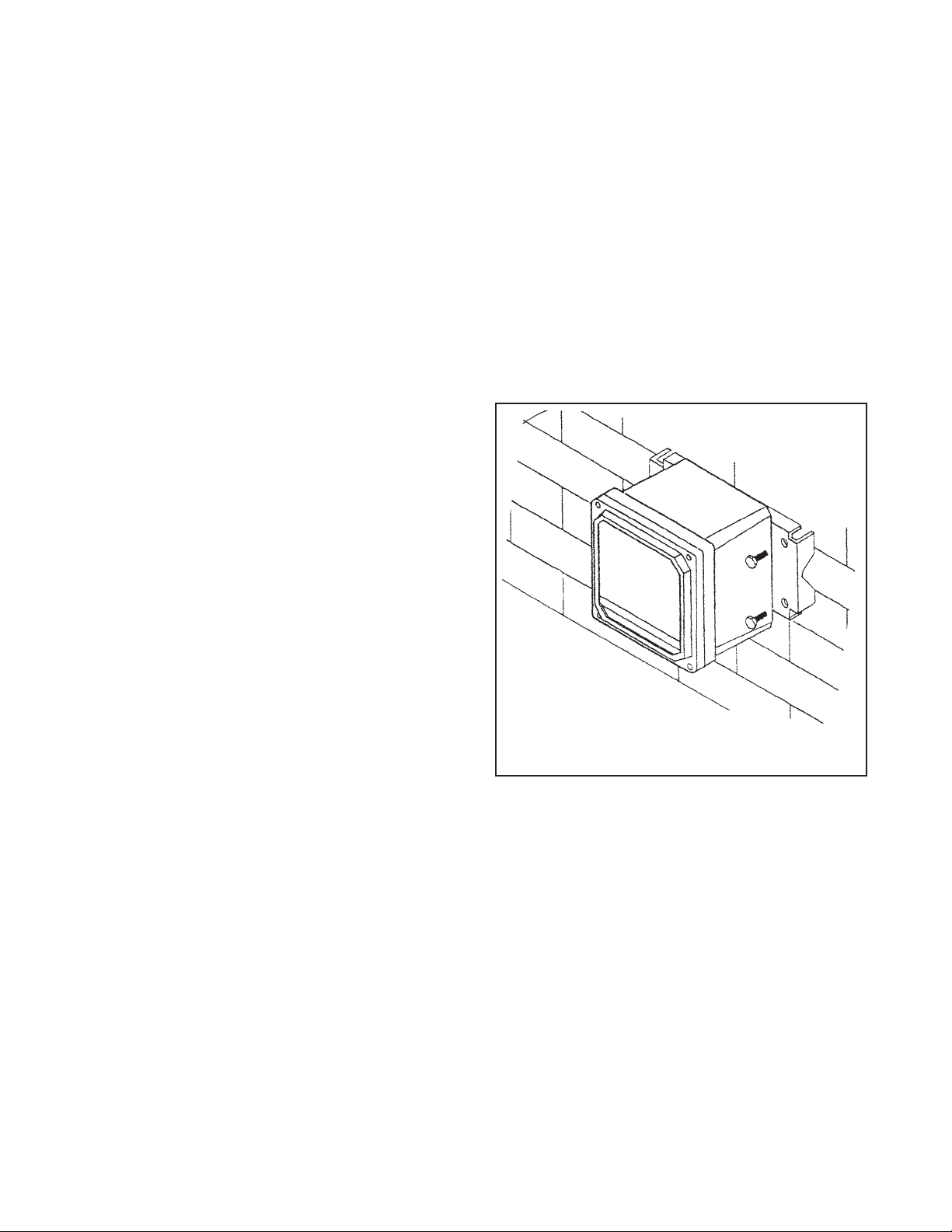
2.3.2 Wall or Surface Mounting:

1. Mount the bracket to the controller using the supplied four screws as shown in Figure 2-2.

2. Mount controller mounting bracket to wall using any appropriate fastener such as screws, bolts, etc (see Figure 2-1 below).

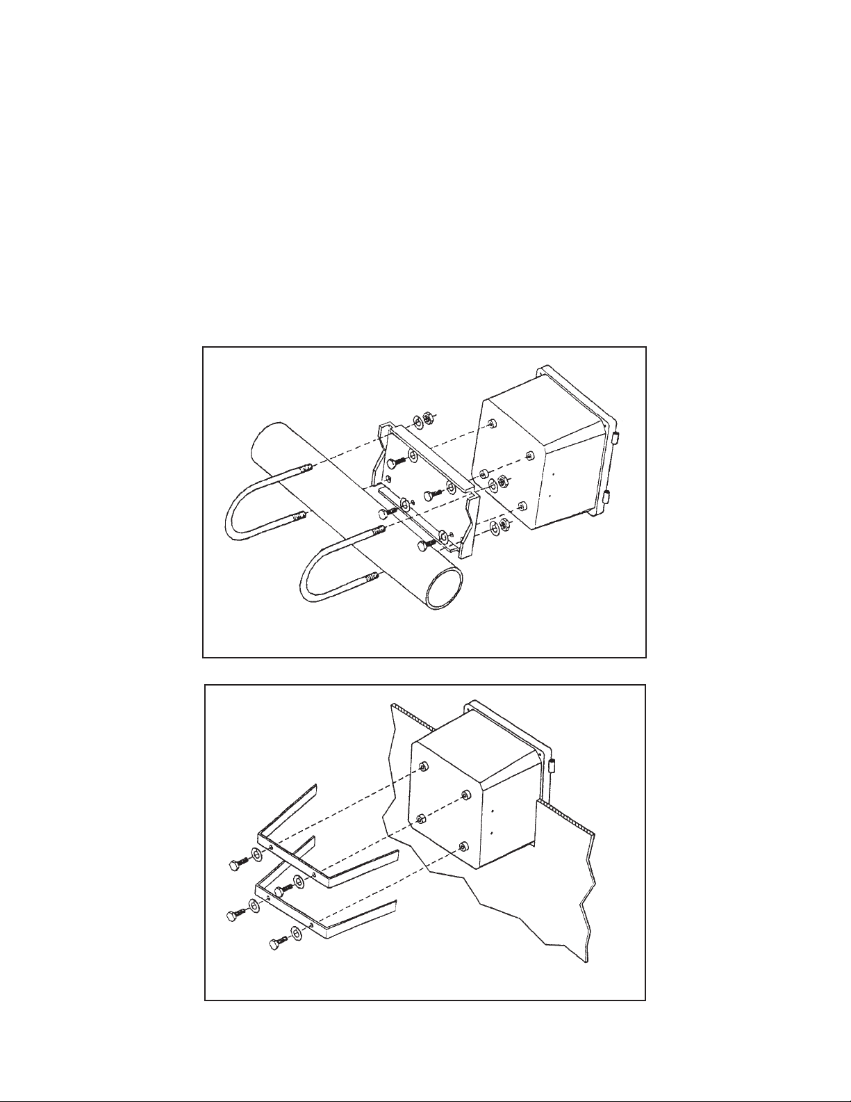
2.3.3 Pipe Mounting:

1. Attach the mounting bracket to the rear of the controller and tighten the four screws as shown in Figure 2-2.

2. Place supplied U bolts around the mounting pipe and through the pipe mounting bracket and mounting bracket. Tighten the U bolt nuts until the controller is securely mounted to the pipe.

FIGURE 2-1. Wall Mounting

FIGURE 2-2. Pipe Mounting

MODEL 54eC SECTION 2.0

INSTALLATION

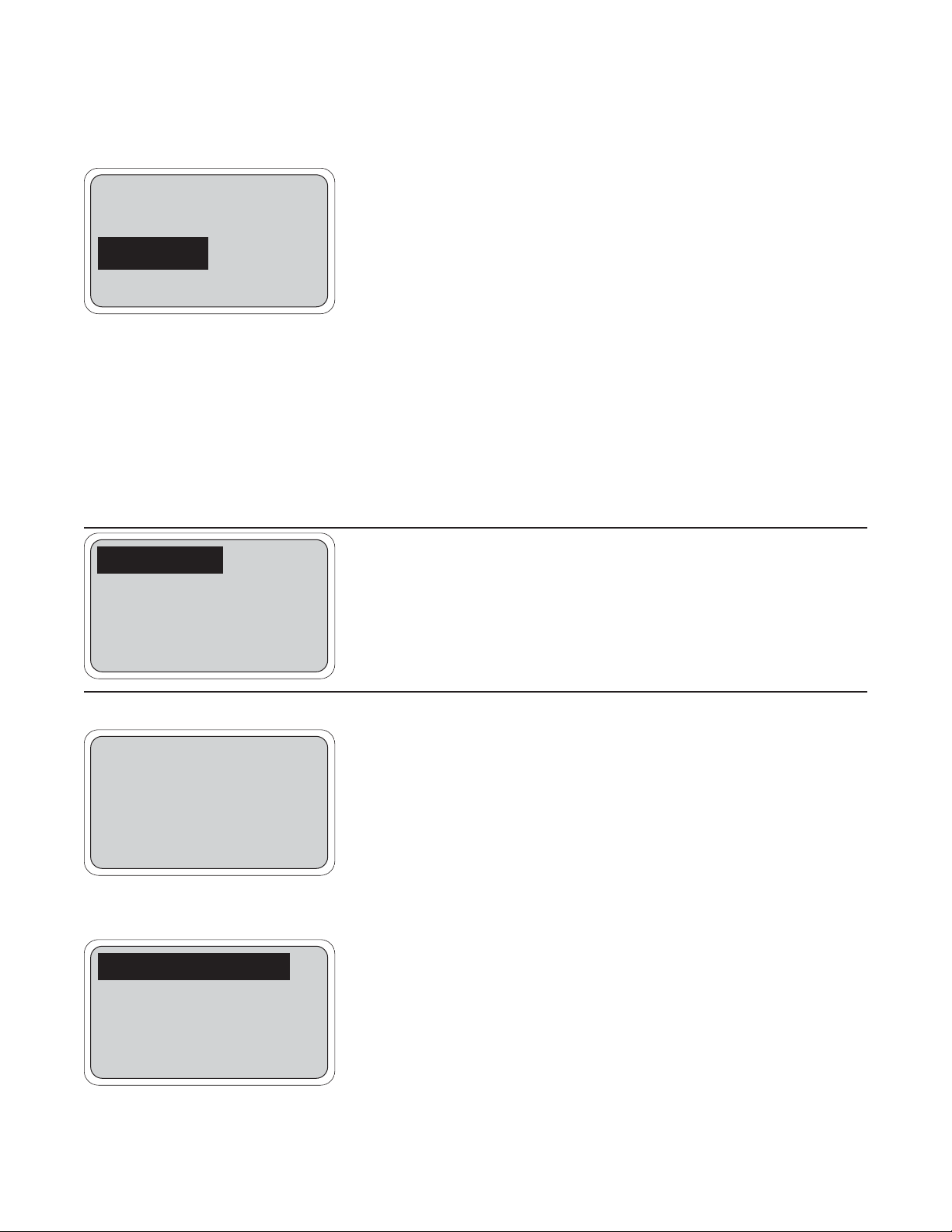
FIGURE 2-3. Panel Mounting

2.3.4 Panel Mounting:

The controller is designed to fit into a 5.43 x 5.43 inch (DIN standard 137.9 x 137.9 mm) panel cutout (Figure 2-3). Installation requires both front and rear access.

1. Install the controller as shown in Figure 2-3. Insert the instrument enclosure through the front of the panel cutout and align the panel mounting brackets as shown.

2. Insert two mounting bracket screws through each of the two mounting brackets and into the tapped holes in the rear of the controller enclosure and tighten each screw.

3. Insert four panel mounting screws through each hole in the mounting brackets. Tighten each screw until the mounting bracket holds controller firmly in place. To avoid damaging the controller mounting brackets, do not use excessive force.

MODEL 54eC SECTION 3.0

WIRING

SECTION 3.0

WIRING

3.1 GENERAL

WARNING

NOTE

Wire only the analog and alarm outputs required for your application. Be sure to read the warning at the beginning of Section 2.0.

The Model 54eC has five access holes in the bottom of the instrument housing which accept ½-in. strain relief connectors or conduit fittings. Be sure to seal any unused access holes. As you face the front of the unit, the rear openings are for input power, and alarm relay signals. The opening on the front left is for sensor wiring only (DC). The front right is for analog output wiring.

NOTE

For best EMI/RFI protection, the output cable should be shielded and enclosed in an earth grounded, rigid, metal conduit. Connect the output cable's outer shield to the earth ground connection on TB2 (Figure 3-1).

3.2 POWER INPUT WIRING

Figure 3-1 depicts the wiring detail for the Model 54eC. Code -01: connect AC power to TB3, terminals 1 and 2 for 115 VAC (terminals 2 and 3 for 230 VAC). Code

-02: connect DC power to TB3 terminals 1, 2, and 3.

Connect earth ground to the nearby ground lug. A good earth ground is essential for proper operation of the controller. Be sure to provide a means of disconnecting the main power to the controller.

CAUTION

Do not apply power to the controller until all electrical connections are made.

WARNING

Electrical connections to this equipment must be made in accordance with the current National and Local Electrical Codes in effect for the installation location.

3.3 ANALOG OUTPUT WIRING

The analog output wiring consists of two 4-20 mA signals: output one from terminals 4 and 5, output 2 from 1 and 2 on TB2, as shown in Figure 3-1. These signals can be used for chart recorder, computer monitoring, or PID control output. The analog outputs can be programmed for 4-20 mA or for 0-20 mA, direct or reverse acting. Current output 1 includes superimposed HART (code -09 only).

3.4 ALARM RELAY OUTPUT WIRING

The controller has 3 "dry" alarm relay contacts which are normally open. Alarm 1 is across terminals 4 and 5 on TB3. This alarm is typically used to control the pump in a chemical feed system. Alarm 2 across terminals 6 and 7 on TB3 is usually used to operate a light or horn as a means of alerting the chemical process operator when conductivity/resistivity/%concentration is outside the control range. Alarm 3 is across terminals 8 and 9 on TB3. All 3 of these alarms may be activated on conductivity/resistivity/%concentration or temperature. They can also be used to control other pumps or valves provided they are programmed to do so. Refer to Section 5.0 to set up these functions.

All three alarm contacts on the Model 54eC are rated for a maximum of 3 A, 115 VAC (1.5A, 230 VAC). If your associated pump or valve exceeds this, use a separate contact or relay rated for the external device.

To use a contact output to control a pump, valve, or light, the contact must be wired into a circuit together with a source of power for the device to be controlled. The power can be jumpered from the main power into the controller and the circuit can be wired as shown on the wiring diagrams, Figure 3-1.

MODEL 54eC SECTION 3.0

WIRING

FIGURE 3-1. Power Input and Relay Output Wiring for Model 54eC

NOTE: Maximum inductive load is 3.0 A at 115 V, 1.5 A at 230V. External power must be brought to relay contact. HART communications superimposed on Output 1.

DWG. NO. REV.

4054EC03 C

MODEL 54eC SECTION 3.0

WIRING

3.5 SENSOR WIRING

Be sure that the conductivity sensor has been properly installed and mounted. Wire the sensor to the junction box (if so equipped) and/or Model 54eC according to Figure 3-2, or use the wiring diagram drawing included inside the controller.

The wiring diagrams show connections between the Model 54eC and the junction box used where distance from the sensor to the controller exceeds the integral sensor cable length and interconnecting wire is required. The interconnecting sensor wire recommended for contacting sensors is PN 9200275. Use of this cable provides EMI/RFI protection and complete sensor diagnostics (for sensors so equipped). The maximum interconnecting wire length is 180 ft. For toroidal sensors, please see sensor manual for recommended interconnecting cable.

IMPORTANT

All interconnecting sensor cable ends must be properly dressed to prevent the individual sensor and shield wires from shorting. All shields must be kept electrically separate all the way back to the terminals on the Model 54eC. Check that there is no continuity between the shield wires and any other sensor conductors or shields prior to connecting the sensor wiring to the terminals on the Model 54eC. FAILING TO FOLLOW THESE INSTRUCTIONS WILL RESULT IN CONTROLLER MALFUNCTION.

3.6 FINAL ELECTRICAL CHECK

CAUTION

To prevent unwanted chemical feed into the process and to prevent injury to operating personnel, disconnect the chemical feed pump and other external devices until the controller is checked out, programmed, and calibrated.

When all wiring is completed, apply power to the controller. Observe the controller for any questionable behavior and remove power if you see a problem. With the sensor in the process, the display will show a conductivity although it may not be accurate.

MODEL 54eC SECTION 3.0

WIRING

FIGURE 3-2. Sensor Wiring Diagram

MODEL 54eC SECTION 4.0

CALIBRATION

SECTION 4.0

CALIBRATION

The following procedures are described in this section:

• Initial Setup (Section 4.1)

• Entering the cell constant (Section 4.2)

• Zeroing the controller (Section 4.3)

• Entering the temperature slope (Section 4.4)

• Standardizing temperature (Section 4.5)

• Standardizing conductivity (Section 4.6)

• Manual Temperature Compensation (Section 4.7)

• Hold Mode (Section 4.8)

NOTE

First Time Users should perform ALL of the procedures in Sections 4.1 to 4.6.

INTRODUCTION

Calibration is the process of adjusting or standardizing the controller to a lab test (such as free acid titration) or a calibrated laboratory instrument, or standardizing to some known reference (such as a commercial chemical standard). Calibration ensures that the controller reads an accurate, and therefore, repeatable reading of conductivity and temperature. This section contains procedures for the first time use and for routine calibration of the Model 54eC controller.

Since conductivity measurements are affected by temperature, the Model 54eC reads the temperature at the probe and compensates for the changing temperature by referencing all conductivity measurements to 25°C (77°F).

To ensure the controller's accuracy, it is important to perform all the calibration procedures provided in this section if you are:

• installing this unit for the first time

• changing or replacing a probe

• troubleshooting

After the initial calibration, the accuracy of the conductivity reading should be checked periodically against some known standard of conductivity and temperature. This is described here and in Section 6.0, Operating Procedures.

WARNINGS

Before performing any of these procedures, be sure to disable or disconnect the chemical feed pumps or other external devices. (see placing controller in hold mode, Section 4.8)

Perform the calibration procedures in this section only in the order they are given. For an introduction to the controller keypad functions, see Section 1.0, Description and Specifications.

Do not attempt to calibrate the controller if the fault LED is lit or the display is showing fault messages. If either of these conditions exist, refer to Section 8.0, Troubleshooting.

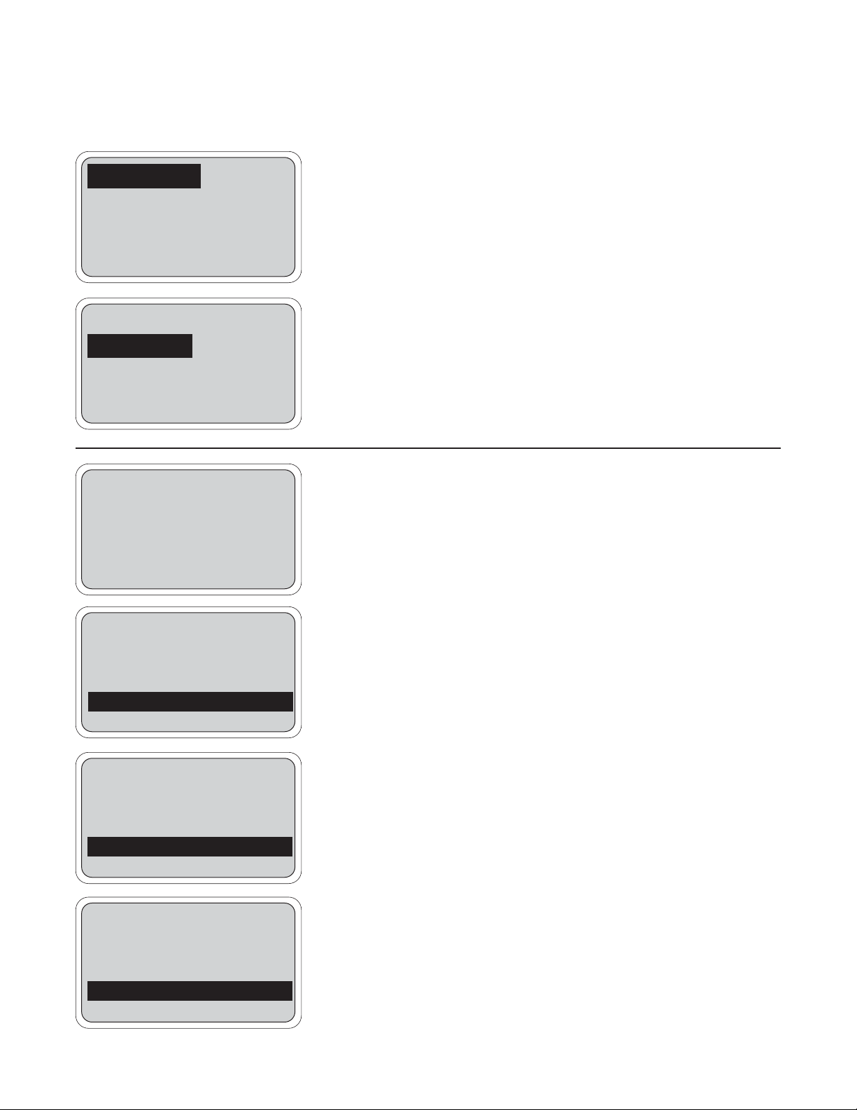
4.1 INITIAL SETUP

MODEL 54eC SECTION 4.0

CALIBRATION

1000

µS/cm

Hold mode: Off

Exit Cont Edit

500

µS/cm

26.2°C. 12.0 mA AL1: 2000μS AL2: 500μS

NOTE

The controller has been configured at the factory for a toroidal sensor ("inductive" mode). If the contacting conductivity probe is used instead, go to Section 5.5 and change the Display Type to "Contacting", BEFORE continuing with Initial Setup here.

The initial setup procedure should be used when first commissioning the controller and when changing the conductivity probe. Some menu headers may appear that are not discussed here, but are included in Section

7.0 as advanced features of the controller that most new users will not need. Initial setup should be conducted with the conductivity probe wired to the controller with full length of extension cable (if any) for best results.

1. From the main display, press any key to obtain the main menu. With

the cursor on "Calibrate", press Enter 4.

NOTE

The hold mode screen (top left) will appear if the hold mode was enabled in Section 5.6. Activate hold mode by pressing Edit 4, using the arrow key to change Off to On, and then pressing Save

4. The hold mode holds the outputs and relays in a fixed state to avoid process upsets to a control system. To leave the hold mode in it's current state, press Cont 3.

2. The display will appear as on the left. Press the down arrow key 3

times to obtain the screen below and press Enter 4 to access the menu for initial setup.

Note that the menu item shown in reverse video is at the bottom of the display. This is the visual cue that you have reached the last menu selection at this level.

Continue the initial setup procedure in Section 4.2

3. To return to the Main Display, keep pressing Exit until the main display appears.

Calibrate sensor

Adjust temperature Temp compensation

Exit Enter

Temp compensation

Initial setup

Output Trim

Exit Enter

MAIN DISPLAY

Calibrate Diagnostic variables Program

Exit Enter

MAIN MENU

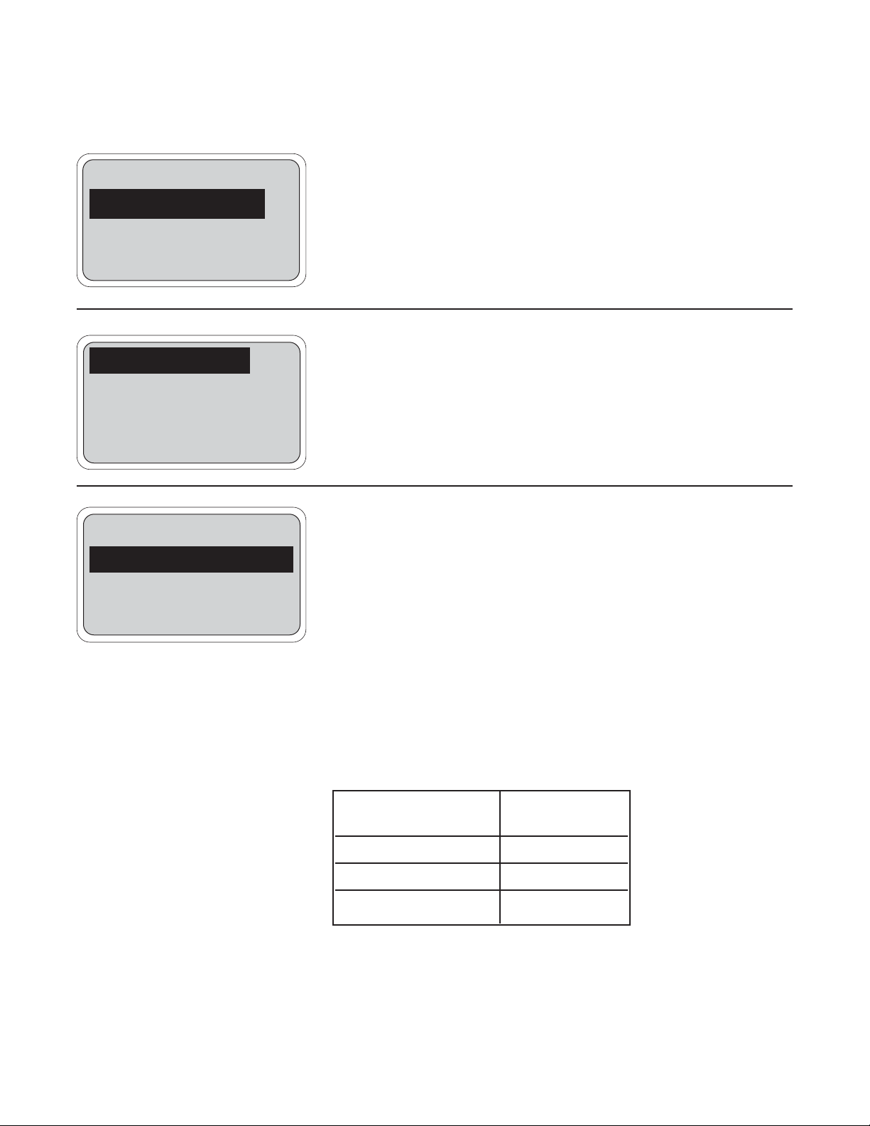
4.2 ENTERING THE CELL CONSTANT

MODEL 54eC SECTION 4.0

CALIBRATION

Adjust temperature Temp compensation

Initial setup

Exit Enter

The cell constant should be entered:

• When the unit is installed for the first time

• When the probe is replaced

• During troubleshooting

This procedure sets up the controller for the probe type connected to the controller. Each type of probe has a specific cell constant:

• Small toroidal (Model 228 or 225) = 3.0

• Large toroidal (Model 226) = 1.0

• Flow-through toroidal (Model 222): 1-inch = 6.0; 2-inch = 4.0

• Low conductivity (contacting sensors) = 0.01 to 10.0

All cell constants can be located on the cable label of the conductivity probe.

1. With the above screen showing on the display, press Enter 4. To get to the above screen, see Section 4.1. Some of the following screens will depend on how the controller was configured in Section 5.5.

2. The screen to the left will be shown.

Press Enter 4 to display or change the cell constant.

3. The display changes as shown on the left. Press Edit 4 to change the indicated cell constant. If the value is correct, press Exit 1.

NOTE

The cell constant you are about to enter is changed after the Standardizing Conductivity procedure is performed (Section 3.6). For inductive sensors and contacting

sensors that only show nominal cell constants, do not change it back to the value on the probe.

The Edit key changes to the Save key and the 3 key now has become the Esc(ape) key. Numerical changes can now be made to the cell constant using the four arrow keys. Once the correct cell constant is shown, press Save 4 to enter the value into memory.

Continue the initial setup by pressing Exit 1 and following directions in Section 4.3.

NOTE

For sensors that show a "cal constant" on the label, the actual cell constant can be calculated adding 500 to the cal constant, multiply this value by the nominal cell constant, then divide the result by 1000.

Cell constant

Sensor zero

Exit Enter

Cell constant 03.00

Exit Edit

Cell constant 01.00

Esc Save

4.3 ZEROING THE CONTROLLER

MODEL 54eC SECTION 4.0

CALIBRATION

This procedure is used to compensate for small offsets to the conductivity signal that are present even when there is no conductivity to be measured. This procedure is affected by the length of extension cable and should always be repeated if any changes in extension cable or sensor have been made. Electrically connect the conductivity probe as it will

actually be used and place the measuring portion of the probe in air.

1. Obtain the screen above (see Section 4.2 for directions) and press the down arrow key to highlight "Sensor Zero".

2. Press Enter 4 to access the zero routine.

3. This display indicates the conductivity reading in air. When in the "Inductive sensor" mode, the reading is displayed to the nearest µS/cm. When configured in the "Contacting sensor" mode, the reading is shown to the nearest .001 µS/cm.

Verify that the sensor is actually in air. If the displayed value is not very close to zero, then press Cont 3 and the controller will establish a new zero. While setting the zero, the message "please wait" is displayed. After a few seconds, the display will return to a value of 0 µS/cm and may then change slightly. A slight variation from zero is to be expected, and the procedure may be repeated several times, if necessary. A successful zero is indicated with a message of "Sensor zero completed"

An unsuccessful zero will result if the conductivity reading is more than 1000 µS/cm or if the reading is too unstable. The "Zero offset error" message indicates the reading is too high for the zero routine. If repeated attempts do not result in an acceptable zero, there is a good chance that there is a wiring problem. Check Section 8.0, Troubleshooting, for help.

Once the reading is close enough to zero, then press Exit 1 and continue initial setup by setting the temperature slope (Section 4.4) or calibrating the temperature reading (Section 4.5).

Cell constant

Sensor zero

Exit Enter

Cell constant

Sensor zero

Exit Enter

5 μS/cm

Sensor Zero Sensor must be in air

Exit Cont

5 μS/cm

Sensor Zero Sensor must be in air

please wait

Exit Cont

2 μS/cm

Sensor Zero Sensor must be in air

Sensor zero completed

Exit Cont

1035 μS/cm

Sensor Zero Sensor must be in air

Zero offset error

Exit Cont

4.4 SELECTING THE TEMPERATURE COMPENSATION TYPE

MODEL 54eC SECTION 4.0

CALIBRATION

Temperature has a significant effect on the conductivity signal. The size of this effect depends on what kind of liquid is being measured. This procedure is used to adjust the type of compensation used by the controller.

1. Obtain the screen above (see Section 4.1 for procedure) and press the down arrow key twice to highlight "Temp compensation".

2. Press Enter 4.

3. Press Edit 4 and use up & down arrow keys to select the appropri- ate temperature compensation: "Linear", "Neutral Salt", or "Cation". If "Linear" is selected, the linear slope may need adjusting (step 4). Press 4 again to select.

For an explanation of the temperature compensation, refer to Section 6.0.

4. The compensation is in the form of a constant slope of 0-5%/°C. Table 4-1 lists some representative values of temperature slopes.The temperature slope currently being used by the controller is shown here. If this value is acceptable, press Exit 1. 2%/°C is a good value for natural waters. For more specialized applications, use the representative values of Table 4-1. To change the temperature slope, press Edit 4.

As before, the Edit key changes to the Save key and the F3 key now has become the Esc(ape) key. Use the four arrow keys to change to the correct temperature slope for your process. Once the correct value is shown, press Save 4 to enter it into memory. Press Esc 3 to cancel.

Adjust temperature

Temp compensation

Initial setup

Exit Enter

Comp type: Linear

Linear slope: 2.00%/°C Auto temp: On

Exit Enter

Comp type: Linear

Linear slope: 2.00%/°C

Auto temp: On

Exit Enter

TABLE 4-1. Typical Temperature Slopes

Chemical Slope (%/°C)

Cleaner (alkaline) 2.25

Cleaner (acid) 1.4

Conversion coating 1.6

4.5 TEMPERATURE CALIBRATION

MODEL 54eC SECTION 4.0

CALIBRATION

This procedure is used to ensure an accurate temperature measurement by the temperature sensor. It enables the controller to display process temperature accurately as well as to compensate for the effect of temperature on the conductivity reading when the temperature in your process changes. The following steps should be performed with the sensor in the process or in a grab sample near the operating temperature.

1. Check the controller temperature reading (main display) to make sure the sensor has acclimated to the process temperature. Compare the controller temperature to a calibrated temperature reading device. Proceed to the next step if the reading requires adjustment.

2. From the main display, press any key and then press Enter 4 to access the Calibrate menu.

NOTE

The hold mode screen may appear (as in Section 4.1) if the hold mode was enabled in Section 5.6. See note on Section 4.1 for instructions.

Press the arrow key once to bring up the screen to the left.

Then press Enter 4.

NOTE

(To verify that the controller is using automatic temperature compensation, highlight the "Temp compensation" menu item and press Enter 4. For more details, see Section 4.7)

3. Press Edit 4 with this display shown to adjust the temperature. The screen below will then appear. Using the arrow keys, input the correct temperature value and press Save 4. The controller will enter the value into memory. To abort the change, press Esc 3. Afterwards, go to Section 4.6 to standardize the conductivity, otherwise press Exit 1 three times for the main display.

NOTE

If hold mode was turned ON, be certain to install the sensor back in the process and change the setting to OFF to resume normal operation before leaving the controller. The Hold screen will appear again before the main display is shown. Follow the same routine as in the Note for Section 4.1 to turn the Hold Mode Off and then press Exit

Calibrate sensor

Adjust temperature

Temp compensation

Exit Enter

25.1 °C

Adjust temp: 25.1°C

Exit Enter

25.1 °C

Adjust temp: +25.1°C

Exit Enter

4.6 CALIBRATING THE SENSOR

MODEL 54eC SECTION 4.0

CALIBRATION

This procedure is used to check and correct the conductivity reading of the Model 54eC to ensure that the reading is accurate. This is done by submerging the probe in the sample of known conductivity, then adjusting the displayed value, if necessary, to correspond to the conductivity value of the sample.

This procedure must always be done after cleaning the probe. The temperature reading must also be checked and standardized if necessary, prior to performing this procedure (see Section 4.5).

Important: If you are submerging the probe in the commercial conductivity standard solution, follow steps 1 through 3. If you are leaving the probe submerged in the bath and checking conductivity against a laboratory instrument skip steps 1-3 and start at step 4.

1. Be sure that the probe has been cleaned of heavy deposits of dirt, oils, or chemical residue.

2. Commercial standards are referenced to a known temperature, for example, 4000 micromhos at 25°C (77°F). As the temperature of the standard changes, the conductivity will change. Therefore it is recommended that this procedure be performed at a temperature between 22 and 28 °C. Be sure the probe has reached a stable

temperature before standardizing.

3. Pour the standard into a clean container. Submerge the clean probe in the standard solution. Place the probe so that a minimum of 1 in. of liquid surrounds the probe. Do not allow the probe to be closer than 1 in. to the sides or bottom of the container. Shake the probe slightly to eliminate any trapped air bubbles. Observe the displayed conductivity to determine if the sensor needs to be moved. Go to step

4. Take a grab sample that is as close to the sensor as possible.

5. Using a calibrated laboratory instrument with automatic tempera- ture compensation, determine the conductivity of the process or grab sample (as close to actual process temperature as possible). Continue with this procedure if an adjustment is needed.

Next, the steps below allow you to change the controller's displayed conductivity reading to match the known value of conductivity of your sample.

6. From the main display, press any key to obtain the main menu. With the cursor on "Calibrate", press Enter 4. Press Enter 4 again when the screen to the left appears.

NOTE

The Hold Mode screen may appear if the feature was enabled in Section 5.6. Changing the Hold Mode to ON holds the outputs in a fixed state, and avoids process upsets during calibration. Remember to change the Hold Mode back to OFF when calibration is completed.

Calibrate sensor

Adjust temperature Temp compensation

Exit Enter

4.6 CALIBRATING THE SENSOR (continued)

4.7 TEMPERATURE COMPENSATION OPTIONS

MODEL 54eC SECTION 4.0

CALIBRATION

7. The conductivity reading in large numbers is the live process reading. The next line displays the conductivity reading when this screen was first accessed. Press Edit 4 to perform the standardize.

Use the arrow keys to change the second line standardize value to the correct conductivity and press Save 4 to complete the procedure. Esc 3 will cancel.

The conductivity reading in the large display will change to the new value and the cell constant or cell factor will be recalculated. The cell factor can be viewed under "diagnostic variables" (Section 8.1).

If too large an adjustment is attempted, the controller will display "standardization error" and no change will be made. See Section 8.0 for troubleshooting.

NOTE

Before exiting the calibration mode, remember to change the hold mode setting to OFF (if it was turned on in step 3).

Automatic Temperature Compensation is a standard option for conductivity equipment and is used in virtually all conductivity measurement situations. If compensation is not desired, the temperature signal from the sensor can be ignored by placing the controller in the manual temperature compensation mode.

Manual mode allows the input of a fixed value that will be used instead of the sensor value. The manual temperature value need only be entered if the temperature compensation setting is manual. In this case, a value may be entered between -15 and 200°C (5 and 392°F).

To change these settings, obtain the top screen by pressing Enter 4 when "Calibrate" is highlighted in the main menu and then press the arrow key b twice. Press Enter 4 again to obtain the lower screen.

Highlight the desired item and press Edit 4 to change the value as needed. Options are Auto or Manual temperature compensation and the temperatures within the range listed above. Press Save 4 to save the change. Esc 3 will cancel the change.

NOTE

When the temperature compensation setting is manual, all temperature specific faults are disabled.

2002

µS/cm

Calibrate: 2000 μS/cm

Exit Edit

1000

µS/cm

Calibrate: 2000 μS/cm

Esc Save

Adjust temperature

Temp compensation

Initial setup

Exit Enter

Auto temp: On

Manual temp: 25.0°C

Ref temp: 25°C

Exit Edit

4.8 HOLD MODE

MODEL 54eC SECTION 4.0

CALIBRATION

Placing the Controller on Hold for Maintenance. Before performing maintenance or repair of the probe, the Controller can be placed in hold (refer to Section 5.6 to enable this feature) to prevent process upsets while the reading is off-line. This will place the current outputs into the selected default states (see Section 5.6). The relays will act as selected in relay default, see Section 5.7.

Before removing the probe from the process, press any key and then Enter 4. When the hold mode has been enabled, the hold mode screen (on the left) will appear prior to calibration. To continue without putting the controller in hold, simply press Cont 3. To put the controller in hold, press Edit 4, use the arrow key to change the "Off" to "On" and press Save 4.

NOTE

When the Hold Mode is Activated (or "On"), the message "Hold Mode Activated" will always appear on the bottom line of the display.

Always calibrate after cleaning or repair of the conductivity probe. After installing the probe back into the process, always change the Hold Mode setting to OFF.

The instrument’s current outputs may be calibrated (trimmed) if necessary. If either the power board or the CPU board is replaced, the outputs must be calibrated. To perform this procedure, a calibrated meter must be connected to the output being calibrated.

To perform an output calibration, from the main display press any key to obtain the main menu. With the cursor on “calibrate,” press Enter (F4). With the cursor on “Output trim,” press Enter (F4) again. Select “Trim output 1” or “Trim output 2” as appropriate.

Press Edit (F4) to select Cal point 1 (4 mA expected and simulated) or Cal point 2 (20 mA expected and simulated). Adjust the Meter value to match the reading of the calibrated meter connected to the output. Press Enter (F4) to complete the calibration.

2002

µS/cm

Hold mode: Off

Exit Cont Edit

2002

µS/cm

26.2 12.0mA

Hold Mode Activated

4.9 TRIM OUTPUTS

Temp compensation Initial Setup

Output trim

Exit Enter

MODEL 54eC SECTION 5.0

SOFTWARE CONFIGURATION

SECTION 5.0

SOFTWARE CONFIGURATION

This section contains the following:

• An introduction to using the configuration process

• A List of Settings for the controller

• Step-by-step instructions and explanations for each parameter on the List

INTRODUCTION TO CONFIGURATION

The controller arrives from the factory configured to work with the inductive (toroidal) conductivity sensor. If

the contacting (electrode) type of sensor will be used, then first go to Section 5.5 and select the appropriate sensor type. If the measurement type is

changed to Resistivity or one of the % concentration choices, then some of the default settings shown in Table 5-1 will also change.

Figure 5-1 is an outline of the menu structure. Before attempting any changes refer to the parameter setup list shown in Table 5-1. This table presents a brief description and the possible options.

The factory setting is listed with a space for the user setting. It is recommended that the list be carefully reviewed before any changes are made.

On initial configuration, it is recommended that the parameters be entered in the order shown on the worksheet. This will reduce the chance of accidentally omitting a needed parameter.

Configuration setups for special applications will be provided as supplements to this manual.

ITEM CHOICES FACTORY SETTINGS USER SETTINGS

PROGRAM LEVEL (Sections 5.1 - 5.3)

A. Alarm Setpoints (Section 5.2)

1. Alarm 1 (low action) 0 - 2,000 mS/cm 1,000 mS/cm _______

2. Alarm 2 (high action) 0 - 2,000 mS/cm 1,000 mS/cm _______

3. Alarm 3 (high action) 0 - 2,000 mS/cm 1,000 mS/cm _______

B. Output Setpoints (Section 5.1, 5.3)

1. Output 1: 4 mA 0 - 2,000 mS/cm 0 mS/cm _______

2. Output 1: 20 mA 0 - 2,000 mS/cm 1,000 mS/cm _______

3. Output 2: 4 mA –25 - 210 °C 0.0 °C _______

4. Output 2: 20 mA –25 - 210 °C 100.0 °C _______

CONFIGURE LEVEL (Sections 5.5-5.7)

A. Display (Section 5.5)

1. Sensor type Inductive/Contacting Inductive _______

2. Measure Resistivity/ConductivityCustom/ 0-15% HCl/98% H2SO4/

0-25% H2SO4/0-12% Na OH Conductivity

3. Temperature Units °C/°F °C _______

4. Output 1 Units mA/% of full scale mA _______

5. Output 2 Units mA/% of full scale mA _______

6. Language

English/Français/Español/Deutsch/Italiano

English _______

7. Display lower left See Section 5.5 Alarm 1 Setpoint _______

8. Display lower right See Section 5.5 Alarm 2 Setpoint _______

9. Display contrast 0-9 (9 darkest) 4 _______

10. Timeout On/Off On _______

11. Timeout Value 1-60 min 10 min _______

12. Polling Address 0-100 0 _______

TABLE 5-1. Conductivity Settings List

Continued on the following page

MODEL 54eC SECTION 5.0

SOFTWARE CONFIGURATION

ITEM RANGES FACTORY SETTINGS USER SETTINGS

B. Outputs (Section 5.6)

1. Output 1 Control

(a) Output Measurement Process/Raw cond/Temperature Process (Cond) _______ (b) Output Control Mode Normal/PID Normal _______

2a. Output 1 Setup (Normal)

(a) Current Range 4-20 mA/0-20 mA* 4-20 mA _______ (b) Dampen 0-299 Sec 0 Sec _______ (c) Hold Mode Last value/Fixed value Last value _______ (d) Fixed Hold Value (if (c) Fixed) 0-22 mA 21 mA _______ (e) Fault value 0-22 mA 22 mA _______

2b. Output 1 Setup (PID)

(a) Setpoint 0-2000 mS/cm or 0-200°C 0 mS/cm _______ (b) Proportional 0-299.9% 100.0% _______ (c) Integral 0-2999 sec 0 sec _______ (d) Derivative 0-299.9% 0.0% _______ (e) LRV (4 mA) 0-2000 mS/cm or 0-200°C 0 mS/cm _______ (f) URV (20 mA) 0-2000 mS/cm or 0-200°C 100 mS/cm _______

3. Output 2 Control

(a) Output Measurement Process/Raw cond/Temperature Temperature _______ (b) Output Control Mode Normal/PID Normal _______

4a. Output 2 Setup (Normal)

(a) Current Range 4-20 mA/0-20 mA 4-20 mA _______ (b) Dampen 0-255 Sec 0 Sec _______ (c) Hold Mode Last value/Fixed value Last value _______ (d) Fixed Hold Value (if (c) Fixed) 0-22 mA 21 mA _______ (e) Fault value 0-22 mA 22 mA _______

4b. Output 2 Setup (PID)

5. Hold (Outputs and Relays) Disable/Enable/ 20 min timeout Disable feature _______

C. Alarms (Section 5.7)

1. Alarm 1 Control

(a) Activation Method Process/Temperature Process _______ (b) Control Mode Normal/TPC Normal _______

2a. Alarm 1 Setup (Normal)

(a) Alarm Logic Low/High/Off High _______ (b) Setpoint 0-2000 mS/cm or 0-200°C 1000 mS _______ (c) Hysteresis (deadband) 0-200 mS/cm or 0-200°C 0 _______ (d) Delay Time 0-99 sec 0 sec _______ (e) Relay Fault Open/Closed/None None _______

2b. Alarm 1 Setup (TPC)

(a) Setpoint 0-2000 mS/cm or 0-200°C 0 mS/cm _______ (b) Proportional 0-299.9% 100.0% _______ (c) Integral 0-2999 sec 0 sec _______ (d) Derivative 0-299.9% 0.0% _______ (e) Time Period 10-2999 sec 30 sec _______ (f) LRV (100% On) 0-2000 mS/cm or 0-200°C 100 mS/cm _______ (g) URV (100% Off) 0-2000 mS/cm or 0-200°C 0 mS/cm _______ (h) Relay Fault None/Open/Closed None _______

TABLE 5-1. Conductivity Settings List (continued)

Continued on the following page

* Option-09, HART-enabled version operates at 4-20 mA only on output 1.

MODEL 54eC SECTION 5.0

SOFTWARE CONFIGURATION

TABLE 5-1. Conductivity Settings List (continued)

ITEM RANGES FACTORY SETTINGS USER SETTINGS

3. Alarm 2 Control

(a) Alarm logic Process/Temperature Process _______ (b) Control Mode Normal/TPC Normal _______

4a. Alarm 2 Setup (Normal)

(a) Configuration Low/High/Off High _______ (b) Setpoint 0-2000 mS/cm or 0-200°C 1000 mS _______ (c) Hysteresis (deadband) 0-200 mS/cm or 0-200°C 0 _______ (d) Delay Time 0-99 sec 0 sec _______ (e) Relay Fault Open/Closed/None None _______

4b. Alarm 2 Setup (TPC)

5. Alarm 3 Control

(a) Alarm Logic Process/Temperature Process _______ (b) Control Mode Normal/TPC Normal _______

6a. Alarm 3 Setup (Normal)

6b. Alarm 3 Setup (TPC)

7. Alarm 4 Setup

(a) Alarm logic Fault/Off Fault _______

8. Feed Limit Timer

(a) Feed Limit Disable/alarm 3/alarm 2/alarm 1 Disable _______ (b) Timeout Value 0-10,800 sec 3600 sec _______

9. Interval Timer

(a) Timer (selection) Disable/alarm 3/alarm 2/alarm 1 Disable _______ (b) Interval 0-999.9 hr 24.0 hr _______ (c) Repeats 1-60 1 _______ (d) On Time 0-2999 sec 120 sec _______ (e) Off Time 0-2999 sec 1 sec _______ (f) Recovery 0-999 sec 600 sec _______

D. Security (Section 3.6)

1. Lock all 000-999 000 (no security) _______

2. Lock Program (Lock all except Calibrate) 000-999 000 (no security) _______

3. Lock Config. (Lock all except Calibrate,

Output setpoints (PID), Simulated Tests Alarm Setpoints, and Rerange Outputs) 000-999 000 (no security) _______

E. Special Substance Calibration (Custom Curve) (Section 7.6)

By changing the standard output configuration, you can set up the Model 54eC to perform a wide variety of control and monitoring tasks. The configuration procedures allow you to program the controller to meet the specific control and monitoring requirements of your particular plant. This is done by recording the desired configuration parameters on the List of Settings Form and then configuring them by using the keys on the controller front panel.

MODEL 54eC SECTION 5.0

SOFTWARE CONFIGURATION

Accessing Calibrate, Program and Configure Menus. Operating configuration changes are made

at the levels shown in Figure 5-1. Pressing any key from the main display will access the main menu (top left).

Level 1 Calibrate. To access calibration selections from the main menu, with the cursor on "Calibrate" press Enter 4. Initial Setup, conductivity standardization and temperature adjustments are made at this level (refer to Section 4.0 for these procedures).

Level 2 Program. To access the program level from the main menu, place the cursor over "Program" with the down arrow key. Then press Enter 4. From the program level menu, changes can be made to the alarm setpoints and the output setpoints.

Level 3 Configure. To access the configure level from the main menu place cursor over "Program" and Enter 4, then place cursor over "Configure" and Enter 4. This level contains advanced selections, such as detailed configuration of current outputs, alarms, and display.

Calibrate

Diagnostic variables Program

Exit Enter

Alarm setpoints

Output setpoints Simulated tests

Exit Enter

Display

Outputs Alarms

Exit More Enter

PROGRAM MENU SECTION

Output Setpoints 5.1 Alarm Setpoints 5.2 Rerange Outputs 5.3 Simulated Tests 5.4

CALIBRATE MENU SECTION

Initial Setup 4.1-4.4 Adjust Temperature 4.5 Standardize Cond 4.6 Temp Compensation 4.7

CONFIGURATION MENU

SECTION

Display 5.5 Outputs 5.6 Alarms 5.7 Security 7.0 Custom Curve 7.6

Security Custom Curve

Factory defaults

Exit More Enter

Calibrate sensor

Adjust temperature Temp Compensation

Exit Enter

Adjust temperature Temp Compensation

Initial setup

Exit Enter

Simulated tests

Configure

Exit Enter

FIGURE 5-1. Outline of Menu Levels

PRESS b TWICE, THEN 4

PRESS

PRESS 4

MODEL 54eC SECTION 5.0

SOFTWARE CONFIGURATION

5.1 CHANGING OUTPUT SETPOINTS (PID ONLY)

This section describes how the two output setpoints can be changed. This selection is only active if the current output control mode has been set to "PID" (see Section 5.6). For reranging normal outputs, go to Section 5.3.

1. From the main display, press any key to obtain the main menu. With

the down arrow key b, move the cursor to "Program" and press Enter 4.

With the cursor on "Output setpoints" (as on the left), press Enter 4.

2. Highlight the desired Output setpoint and press Enter 4.

3. The setpoint now being used is displayed. If the control mode is set

to "Normal", "setpoint" will not be displayed. Press Edit 4 and use the arrow keys to change the display to the new value.

4 mA is the deviation from setpoint that will result in a 4 mA out. 20 mA is the deviation from setpoint that will result in a 20 mA setpoint. Highlight the desired item and press Edit 4 and the arrow keys to change the display to the new value.

Example: A setpoint of 500 μS/cm with a URV of +1000 μS/cm and a LRV of 0.0 μS/cm. When the conductivity is 1000 μS/cm, the output will be (1000-500)/(1000-0) = 50% of range (12 mA). If the setpoint is changed to 1500 μS/cm, the output will be (1500-1000)/(1000-0) = 25% of range (8 mA).

4. Press Save 4 to enter into memory or Esc 3 to abort the change.

The Control setpoint is typically the condition where the current output is at a minimum. The P and I control calculations use the setpoint to adjust the current output to the desired level based on the parameters established in Section 5.6.

Alarm setpoints

Output setpoints

Simulated tests

Exit Enter

Output 1 setpoints

Output 2 setpoints

Exit Enter

Setpoint: 1000 μS/cm 4 mA: 0.0000 μS/cm 20 mA: 1000 mS/cm

Exit More Enter

Setpoint: 1000 μS/cm

4 mA: 0.0000 μS/cm 20 mA: 1000 mS/cm

Exit More Enter

MODEL 54eC SECTION 5.0

SOFTWARE CONFIGURATION

5.2 CHANGING ALARM SETPOINTS

This section describes how the three alarm setpoints can be changed.

Move the cursor down by pressing the arrow b key.

1. From the main menu, move the cursor down to "Program" and press

Enter 4. On the next display, move the cursor to "Alarm setpoints" and press Enter 4.

2. Select the desired alarm by moving the cursor down to highlight it.

When the correct alarm is highlighted, press Enter 4 to get to the adjustment screen.

In this example we have pressed the arrow key down once to access

the alarm 2 setpoint.

NOTE

There are 2 different possible screens at the next point, depending on whether the alarm has been configured as normal or TPC.

3a. (normal alarm). The setpoint now being used for this alarm and the

kind of alarm (high or low) are displayed. (If the alarm has been turned off, then "off" will be displayed instead of "High") The "Enter" key has now changed to the "Edit" key and will allow changing the setpoint once the F4 key has been pressed. If the setpoint is ok, then press Exit 1.

After the Edit 4 key is pressed, use the arrow keys to change the display to the desired setpoint and press Save 4 to enter into memory. The plus (+) sign can be changed to a minus sign by pressing the down arrow key when the (+) is highlighted. To abort the change, press Esc 3 to return to the previous menu.

3b. (TPC alarms only). When the alarm has been configured as TPC,

the setpoint is used for the TPC calculation of how long the alarm should stay on. The "Enter" key has now changed to the "Edit" key and will allow changing the setpoint once the F4 key has been pressed. If the setpoint is ok, then press Exit 1.

After the F4 key is pressed, use the arrow keys to change the display to the desired setpoint and press Save 4 to enter into memory. The plus + sign can be changed to a minus sign by pressing the down arrow key. To abort the change, press Esc 3 to return to the previous menu.

NOTE

This alarm setpoint will replace the 0% On point entered in Section 5.7. The 100% On point will also be moved to preserve the exact same range of operation. This kind of action is referred to as a "sliding window". Refer to Section 6.0 for more technical details.

Alarm setpoints

Output setpoints Simulated tests

Exit Enter

Alarm 1 setpoint

Alarm 2 setpoint

Alarm 3 setpoint

Exit Enter

Alarm High: 2000 μS/cm

Exit More Enter

Setpoint: 1500 μS/cm

Exit More Enter

MODEL 54eC SECTION 5.0

SOFTWARE CONFIGURATION

5.3 CHANGING OUTPUT SETPOINTS (NORMAL)

This section describes how the 4 (or 0) to 20 mA current outputs can be reranged. Note that the current outputs can be configured to represent conductivity (or resistivity), raw conductivity, % concentration, or temperature.

See Section 5.6 for details on configuration.

1. From the main menu, move the cursor down to "Program" and press

Enter 4. On this display, move the cursor to "Output setpoints" and press Enter 4.

Note: 0-20 mA output range is disabled on output 1 with HARTenabled version (-09 option).

2. Select the desired output by moving the cursor down to highlight it.

When the correct output is highlighted, press Enter 4 to get to the adjustment screen.

3. This message asks for confirmation of the requested change. Changes in these settings may degrade process control, so use caution when making changes. Press Cont 3 to continue. Otherwise press Abort 1.

This screen allows changing the setpoints for output 1. A similar screen is available for output 2. The live current output now being transmitted by the controller is shown on the third line.

4. Press Edit 4 to make changes in the setpoints. The Edit key changes to a Save key and the F3 key becomes active as an Esc key. Use the arrow keys to make the display read the desired values for the high and low current output limits. When done, press Save 4 to enter the changes into memory. Press Esc 3 to cancel changes.

NOTE

Outputs that have been configured as 0-20 mA in Section 5.6, will show 0 mA instead of 4 mA on the top line. Outputs that are based on temperature or resistivity values will show matching units such as °C or MΩ-cm. See Section 5.6 for output configuration.

Alarm setpoints

Output setpoints

Simulated tests

Exit Enter

Output 1 setpoints

Output 2 setpoints

Exit Enter

4 mA: 0 mS/cm 20 mA: 2000 mS/cm Output 1: 12.00 mA

Exit Edit

CAUTION: Current output 1 will be affected.

Abort Cont

4 mA: +0000 mS/cm

20 mA: 2000 mS/cm Output 1: 12.00 mA

Esc Save

MODEL 54eC SECTION 5.0

SOFTWARE CONFIGURATION

5.4 TESTING OUTPUTS AND ALARMS

This section describes how the current outputs and alarm relays can be manually set for the purposes of checking devices such as valves, pumps, or recorders.

1. From the main menu, move the cursor down to "Program" and press Enter 4. On this display, move the cursor to "Simulated tests" and press Enter 4.

2. At this point there are six separate screens for testing each of the current outputs and each of the alarm relays. Highlight the desired item by pressing the arrow b t keys as needed.

When the desired item is highlighted, press Enter 4 to continue. Go to step 3a for outputs and 3b for alarms.

NOTE

A cautionary message will appear to warn that the output or alarm that was selected will be changed by the following action. Be sure to alert plant personnel that these changes are simulated and do not represent a change in the actual process. Press Cont 3 to continue or Abort 1 to cancel the simulation.

3a. The output is now being simulated. In the example to the left, out-

put 1 has been set to 10.00 mA. The output will remain at 10.00 mA until either Exit 1 (or Edit 4 see below) is pressed or the test is concluded by timeout. The default value for the timeout is 10 minutes, so after 10 minutes, the output would go back to normal operation. To configure the timeout option, see Section 5.5.

If the displayed current is not the desired value, press the Edit 4 key and the next screen will allow changing the value. Use the arrow keys to change the display as needed, and press Test 4 to use that value. Press Esc 3 to cancel the change in the value and continue simulating the previous current.

Output setpoints

Simulated tests

Configure

Exit Enter

Test output 1

Test output 2 Test alarm 1

Exit Enter

Test alarm 2 Test alarm 3 Test alarm 4

Exit Edit

MODEL 54eC SECTION 5.0

SOFTWARE CONFIGURATION

5.4 TESTING OUTPUTS AND ALARMS (continued)

3b. The alarm relay is now being simulated. In the example to the left,

alarm 1 has been set to Open. This means that the relay is not energized (i.e. off). The alarm will remain open until either Exit 1 or Edit 4 is pressed or the test is concluded by timeout. The default value for the timeout is 10 minutes, so after 10 minutes, the alarm would go back to normal operation and the display will return to the main menu. To configure the timeout option, see Section 5.5.

If the displayed alarm action is not as desired, press the Edit 4 key and the next screen will allow changing it. Use the arrow keys to change the display as needed, and press Test 4 to enter the change. Press Esc 3 to cancel the change in the value and continue simulating the previous action.

NOTE

Alarm relays may be simulated in the energized (Closed) position or the de-energized (Open) position.

Test alarm 1: Open

Exit More Enter

Test alarm 1: Open

Simulating alarm1

Exit Edit

MODEL 54eC SECTION 5.0

SOFTWARE CONFIGURATION

5.5 CHOOSING DISPLAY OPTIONS

This section describes the options available for the changing of engineering units and variables on the main display.

1. From the main menu, move the cursor down to "Program" and press Enter 4. From the program menu, move the cursor down using the arrow key to highlight "Configure" and press Enter 4.

The first configuration menu is displayed. With the cursor on "Display" press Enter 4.

2. Menu Item Options

Sensor Inductive/Contacting

Measure Conductivity/Resistivity/Custom%/

0-15% HCl/98% H2SO4/

25% H2SO4/ 0-12% NaOH

Temperature units °C/°F

The values now being used by the controller are displayed. To change any of these items, use the arrow key to highlight the desired item and press Edit 4. Use the arrow keys to make the change and press Save 4 to enter the change into memory. Applications using the toroidal probe should always use the "Inductive" setting. Applications using probes with exposed electrodes should use the "Contacting" setting. Note that all these measure choices are referred to as "Process" by the controller and in other places in this manual. See Sections 6.0 and 7.0 for measure explanation.

MEASURE WARNING

Changing the measurement selection will cause the controller to reset alarm and output setpoints to new measure units. Press Abort 1 to cancel the change. Press Cont 3 to change the measurement.

3. Menu Item Options

Output 1 units mA/percent

Output 2 units mA/percent

LanguageEnglish/Français/Español/Deutsch/Italiano

Press the arrow key four times to access this screen. The current outputs can be displayed as milliamps or as percent of full scale. The default is mA. To change any of these items, use the arrow key to highlight the desired item and press Edit 4. Use the arrow keys to make the change and press Save 4 to enter the change into memory.

Further menu items are available by pressing the arrow b key repeatedly. When the display is highlighting the item on the third line, the end of the menu has been reached. To back up within the menu, use the up t arrow key.

Display

Outputs Alarms

Exit Enter

Sensor: Inductive Measure: Conductivity Temp units: °C

Exit Enter

Output 1: mA

Output 2: mA

Language: English

Exit Edit

Display left: AL1

Display right: AL2

Display contrast: 5

Exit Edit

WARNING: This change resets analyzer to factory settings

Abort Cont

MODEL 54eC SECTION 5.0

SOFTWARE CONFIGURATION

5.5 CHOOSING DISPLAY OPTIONS

4. This screen allows you to choose the items displayed on the third line left and right of the main display screen. The process temperature and output 1 value (in mA or %) are always shown on line 2 of the main display. This screen allows you to make the following choices:

Lower Left of Main Display Lower Right of Main Display

• AL 1 (alarm 1 setpoint-no units shown) • AL 2 (alarm 2 setpoint-no units shown)

• AL 3 (alarm 3 setpoint-no units shown) • AL 3 (alarm 3 setpoint-no units shown)

• RAW (uncompensated conductivity) • RAW (uncompensated conductivity)

• Blank (nothing displayed in lower left) • Out 2 (Output 2 value in mA or %)

• Blank (nothing displayed in lower right)

The "Display contrast" selection allows the display to be made lighter or darker. Entry 0 is the lightest and 9 is the darkest. The display changes as the number is changed.

To change any of these items, use the arrow key to highlight the desired item and press Edit 4. Use the arrow keys to make the change and press Save 4 to enter the change into memory. Press Esc 3 to abort.

NOTE

The display can also be changed by holding down the F3 key while pushing the down key to increment through the display levels.

5. The timeout feature works on both the display and simulated tests using the current outputs and alarm relays.

The display timeout will return the display to the main display screen (from any other screen) if no key is pressed before the timeout value. This is useful because the main display screen is usually the most important screen to the operator.

The timeout feature also allows simulating the current output and alarm actions with an automatic return to normal operation. When the feature is turned on (the default), simulated tests (see Section 5.4 for details) will be completed automatically when the timeout value is reached.

As before, to change these settings, use the arrow key to highlight the desired item and press Edit 4. Use the arrow keys to make the change and press Save 4 to enter the change into memory. Press Esc 3 to abort.

SECURITY CAUTION

The Timeout Value is also used by the controller to activate security (Section 7.0). After unlocking the controller by entering a security code, security is not re-activated unless a display timeout occurs. If Timeout has been turned off here, security will never re-activate.

Display left: AL1

Display right: AL2

Display contrast: 5

Exit Edit

Display left: AL1

Display right: AL2

Display contrast: 5

Esc Save

Display contrast: 5 Timeout: On

Timeout Value: 10 min

Exit Edit

MODEL 54eC SECTION 5.0

SOFTWARE CONFIGURATION

5.6 CHANGING OUTPUT PARAMETERS

This section describes the options available for configuration of the outputs. Each output can be configured to represent conductivity (or resistivity see Section 5.5), raw conductivity, % concentration, or temperature. In addition, each output can be linear (normal) or nonlinear (PID). Several options for both modes of outputs can be configured. This section describes the features and shows how to make modifications in the settings.

1. Beginning from the main menu, move the cursor down to "Program" and press Enter 4. From the program menu, move the cursor down using the arrow key b to highlight "Configure" and press Enter 4.

Use the arrow key again to highlight "Outputs" (as shown on the left) and press Enter 4.

2. There are 5 menu headers that relate to outputs. Each output has a control header and a setup header. In addition, the hold feature is turned on here. The hold feature is mostly used to prevent upsets during calibration of the conductivity probe in a standard solution.

To access each header, highlight the desired item and press the Enter 4 key. To select another header, use the arrow keys. The bottom menu header will only be highlighted if the end of the menu has been reached.

NOTE

Always configure the control parameters BEFORE making changes in the output setup. Changes in the output setup in step 4 will depend on the options that have been selected in step 3.

3. Menu Item Options

Output Measurement Process/Raw Cond/Temperature

Control Mode Normal/PID

Each output can be configured with the options above. The default options are that output 1 is Process (conductivity or resistivity), output 2 is Temperature and that both outputs are Normal (not PID). This is the most common configuration and may not require changes. If no changes are desired, skip to step 4.

To make changes in these parameters, highlight the desired menu header and press Enter 4. The value now being used is displayed and the F4 key can be pressed to Edit the item. Once Edit has been pressed, change the item as needed and then press Save 4 to store the value. Repeat for the other output and/or items as needed.

Output 1 control

Output 1 setup Output 2 control

Exit Enter

Output Measurement

Control Mode

Exit Enter

Output: Process

Exit Edit

Display

Outputs

Alarms

Exit Enter

Output 2 control Output 2 setup

Hold feature setup

Exit Edit

Output Control Parameters

MODEL 54eC SECTION 5.0

SOFTWARE CONFIGURATION

5.6 CHANGING OUTPUT PARAMETERS (continued)

4a. Menu Item Options

Range 4-20mA/0-20mA

Dampen(ing) 0-299 sec

Hold Last value/fixed value

Fixed Hold (if Output 1 hold is "fixed value") 0-22.00 mA

Fault (fixed value in a fault condition) 0-22.00 mA

Note: 0-20 mA output range is disabled on output 1 with HART-enabled verion (-09 option).

These parameters can be adjusted by highlighting the desired item and pressing the Edit 4 key. Once Edit has been pressed, change the item as needed and then press Save 4 to store the value.

"Range" determines whether the 4-20mA or 0-20 mA convention is used for the current output. If the range is changed, be sure to rerange the outputs as described in Section 5.3.

"Dampening" is used to time-average the current output, smoothing out the effect of a noisy reading. Higher values provide more smoothing.

Enabling the "hold" feature will give the user the option of placing the output in hold during the calibration sequence.

A "fixed value" places the held output at a fixed value between 0 and 22 mA.

4b. Menu Item Options

Set point 0 to 2000 mS/cm (Inductive, Contacting),

0.055µS/cm to 20 mS/cm (Ultrapure), 50 Ω-cm to 20 MΩ-cm (Resistivity),

0 to 100°C (Temperature)

Proportional 0-299.9 %

Integral 0-2999 sec

Derivative 0-299.9 %

The four parameters above are only available for outputs that have been configured as PID outputs in step 3. These parameters can be adjusted using the same technique as in step 4a, by highlighting the desired item and pressing the Edit 4 key. Once Edit has been pressed, change the item as needed and then press Save 4 to store the value.

Use caution in changing the values of these parameters.

"Setpoint" is usually the desired value at which the process is being controlled, typically the output will be 4(or 0) mA when the parameter is near the setpoint. This setting can also be changed using the procedure in Section 5.1.

Range: 4-20 mA

Dampen: 0 sec Hold: Last Value

Exit Edit

Output Setup Parameters (for Normal Outputs)

Setpoint: 1000 μS/cm

Proportional: 100.0% Integral: 0 sec

Exit Edit

Output Setup Parameters (for PID Outputs only)

Derivative: 0.0%

Range: 4-20 mA

Hold: Last Value

Exit Edit

Fixed Hold: 21.00mA

Fault: 22.00mA

Exit Edit

MODEL 54eC SECTION 5.0

SOFTWARE CONFIGURATION

"Proportional" is short for Proportional Band and indicates the range

over which control is being used. It is the opposite of the process gain. Smaller values provide tighter control.

"Integral" is the number of seconds over which deviations from the setpoint are integrated to remove continuing offsets. Smaller values provide higher response.

"Derivative" is a form of control that resists all changes in readings. Higher readings increase the derivative function. Use caution in setting the derivative value to prevent process oscillation.

More information regarding PID control can be found in Section 7.0. Setting these parameters may require some trial and error and should be tested while the process is being supervised to prevent future upsets.

The rest of the PID output setup parameters are identical to those used for normal outputs. See step 4a for details .

5. The Hold feature is used to prevent problems that may occur during calibration if the current outputs are used for control. The feature is turned on (enabled) here and is specifically configured in step 4. The controller starts out with the hold feature turned off (disabled).

To enable the Hold feature, obtain the screen to the left with the hold feature setup highlighted (see steps 1 and 2 for exact instructions). Press Enter 4 and the screen below will appear.

Press the Edit 4 key to enable changes. Options include Disable, Enable, and 20 minute timeout. When 20 minute timeout is selected, the hold mode will automatically disengage after being on for 20 minutes. Selecting Enable or 20 minute timeout does not actually put the controller in hold, but rather allows putting the controller in hold when calibration is conducted.

When the hold feature has been enabled, this Hold Mode Screen will appear when the Calibrate routine is entered. Possible actions are Exit 1 which cancels the calibration, Cont 3 which enters the calibrate menu without putting the controller in hold, and Edit 4 which allows turning Hold Mode On. Note that when hold has been enabled, this screen requires pushing Cont 3 to enter and leave the calibrate menu.

Fixed Hold: 21.00mA

Fault: 22.00mA

Exit Edit

Output 2 control Output 2 setup

Hold feature setup

Exit Enter

Hold: Disable feature

Exit Edit

Hold Feature Setup

1000

µS/cm

Hold mode: Off

Exit Enter

5.6 CHANGING OUTPUT PARAMETERS (continued)

MODEL 54eC SECTION 5.0

SOFTWARE CONFIGURATION

5.7 CHANGING ALARM PARAMETERS

This section describes the options available for configuration of the alarms. Alarms 1, 2, and 3 can be activated on Conductivity (or resistivity, see Section 5.5), or temperature. One of these alarms can be setup as a feed limit timer and another alarm can be dedicated as an interval timer. Alarm 4 is reserved as a fault alarm.

Alarms that activate on conductivity (or resistivity) or temperature can be configured as on/off (normal) or TPC. These modes are described below. Each of these alarm modes have several configuration options that are described in detail in this section.

1. Beginning from the main menu, move the cursor down to "Program" and press Enter 4. From the program menu, move the cursor down using the arrow key b to highlight "Configure" and press Enter 4.

Use the arrow key again to highlight "Alarms" (as shown on the left) and press Enter 4.

2. There are 9 menu headers that relate to alarms. Alarms 1, 2, and 3 each have a control header and a setup header. Alarm 4 has a simple setup header. Configuration of a feed limit timer and an interval timer is also described here.

NOTE

Always configure the control parameters BEFORE mak- ing changes in the alarm setup. Changes in the output setup in step 4 will depend on the options that have been selected in step 3.

Alarm Modes:

Normal: Alarm turns on when setpoint is exceeded and turns off when the reading no longer exceeds the setpoint (simple high alarm example).

Fault: Alarm turns on when controller detects a fault condition.

TPC: Alarm turns on for a time that depends on what the reading is. The time it stays on is proportional to how far the reading is from the 0% On Time point, also called the setpoint. (time proportional control)

TPC(PID): Alarm is a TPC alarm, but the amount of time it stays on depends not only on how far the reading is from a setpoint, but also on how long it has exceeded the setpoint, and how fast it has actually changed. (Proportional Integral Derivative control)

Feed limit timer: When the alarm has been energized (on) for a long period, it automatically turns off to prevent overfeeding of chemicals.

Interval timer: Alarm is programmed to activate at various times, usually to provide automated cleaning. Useful for spray cleaning and/or automatic retraction of sensors in processes.

Alarm 1 control

Alarm 1 setup Alarm 2 control

Exit Enter

Outputs

Alarms

Security

Exit Enter

Alarm 2 setup

Alarm 3 control

Alarm 3 setup

Exit Enter

Alarm 4 setup Feed limit timer

Interval timer

Exit Enter

MODEL 54eC SECTION 5.0

SOFTWARE CONFIGURATION

5.7 CHANGING ALARM PARAMETERS (continued)

Alarm Control Parameters

Alarm Setup Parameters (for Normal Alarms only)

3. Menu Item Options

Activation Method Process/Temperature

Control Mode Normal/TPC

Alarms 1, 2, and 3 can each be configured with the options above. The default options are that all three alarms are Process (conductivity, resistivity or % concentration), and Normal (not TPC). This is a common configuration and may not require changes. If no changes are desired, skip to step 4a.

To make changes in these parameters, highlight the desired menu header and press Enter 4. The value now being used is displayed and the F4 key can now be pressed to Edit the item. Once Edit has been pressed, change the item as needed and then press Save 4 to store the value. Repeat for the other output and/or items as needed.

NOTE

An alarm that has been dedicated as an Integral Timer will not have a Control Mode option and will display "Not Applicable".

4a. Menu Item Options

Alarm (action) Low/High/Off

Setpoint 0 - 2000 mS/cm, 0 to 200°C.

Hysteresis 0 - 2000 mS/cm, 0 to 10°C.

Delay 0-99 sec

Relay default None/Close/Open

These parameters can be adjusted by highlighting the desired item and pressing the Edit 4 key. Once Edit has been pressed, change the item as needed and then press Save 4 to store the value.

"Alarm action" determines whether alarm will activate when the reading exceeds the setpoint (high alarm) or when it drops below the setpoint (low action). It can also be turned off (i.e. not used).

"Hysteresis" is a deadband that prevents deactivating a relay until the reading has dropped below the setpoint minus the hysteresis amount (high alarm example).

"Delay" will delay activation (and deactivation) of the relay for a certain number of seconds. Larger delays can reduce relay chatter.

"Relay Default" determines how the relay will act if there is a fault or hold condition. Each alarm can be forced on (Close), off (Open) or can remain unchanged (None). The factory configuration is "None".

Activation Method

Control Mode

Exit Enter

Activate: Process

Exit Edit

Alarm: Low

Setpoint: 1.000 mS/cm Hysteresis: 0 mS/cm

Exit Enter

Hysteresis: 0.00% Delay: 0 sec

Relay Default: None

Exit Enter

MODEL 54eC SECTION 5.0

SOFTWARE CONFIGURATION

5.7 CHANGING ALARM PARAMETERS (continued)

Alarm Setup Parameters (for TPC Alarms)

4b. Menu Item Options

Setpoint 0 to 2000 mS/cm (Inductive,Contacting),

50 Ω-cm to 20 MΩ-cm (Resistivity),

full % concentration range,

0 to 100°C (Temperature)

Proportional 0-299.9 %

Integral 0-2999 sec

Derivative 0-299.9 %

Time period 10-2999 sec

URV (100% On) 0 to 2000 mS/cm (Inductive,Contacting), LRV (0% On) 0.055 µS/cm to 20 mS/cm (Ultrapure),

50 Ω-cm to 20 MΩ-cm (Resistivity),

0 to 100°C (Temperature)

Relay Default None/Close/Open

These parameters are available for alarms that have been configured as TPC alarms in step 3. Parameters can be adjusted using the same technique as in step 4a, by highlighting the desired item and pressing the Edit 4 key. Once Edit has been pressed, change the item as needed and then press Save 4 to store the value.

"Setpoint" is usually the desired value at which the process is being controlled, typically the alarm will not be on very much when the process is at this value. This setpoint is also accessible in the Program Menu under "Alarm Setpoints" (see Section 5.2)

"Proportional" is short for Proportional Band and indicates the range over which control is being used. It is the opposite of the process gain. Smaller values provide tighter control.

"Integral" is the number of seconds over which deviations from the setpoint are integrated to remove continuing offsets. Smaller values provide higher response.

"Derivative" is a form of control that resists all changes in readings. Higher readings increase the derivative function. Use caution in setting the derivative value to prevent process oscillation.

"Time period" is the cycle time for the TPC control. One cycle consists of an energized (relay on) time and an deenergized (relay off) time. The relative amounts of on time and off time depends on the reading and the other settings listed here.

"100% On" is the deviation from the setpoint that results in the alarm being on all the time.

"0% On" is the deviation from the setpoint that results in the alarm being off all the time. This is generally set to zero.

"Threshold" is the minimum deviation from the setpoint that will result in some amount of on time. Until the process value crosses this threshold, the alarm will not be energized even if it would be based on the setpoint and 0% On, 100% On times that are being used.

Setpoint; 500 μS/cm

Proportional: 100.0% Integral: 0 sec

Exit Edit

Derivative: 0.0%

Time period: 30 sec

100% On: 1000 μS/cm

Exit Enter

% On: 0 μS/cm Threshold: 0 μS/cm

Relay default: None

Exit Enter

MODEL 54eC SECTION 5.0

SOFTWARE CONFIGURATION

5.7 CHANGING ALARM PARAMETERS (continued)

"Relay Default" determines how the relay will act if there is a fault or

hold condition. Each alarm can be forced on (Close), off (Open) or can remain unchanged (None). The original configuration is "None". A TPC relay set at "None" will remain open or closed until the fault or hold condition is over.

CAUTION

Understanding how to set TPC settings is not trivial and is likely to require substantial trial and error to yield acceptable results. Applying PID algorithms to conductivity and resistivity measurements can result in unintended effects.

More details regarding PID control can be found in Section 7.0.

5. Alarm 4 is dedicated as a fault alarm. The only option for this alarm is to enable it or to disable it. To disable the alarm, press Edit 4 and use the arrow key to change "Fault" to "Off" .

When a fault condition exists, the relay will energize and the red LED on the front display will turn on.

EXAMPLE 1: A setpoint of 500 µS/cm with 100% On of +1000 µS/cm and 0% On of 0.0 µS/cm, a time peri-

od of 30 seconds, and a threshold of 0.0 µS/cm. When the Conductivity is 1000 µS/cm, the relay will be on (1000-500)/(1000-0) = 50% of the time. This alarm will act just like Example 1 in the previous TPC section.

Alarm 4 Setup

Alarm: Fault

Exit Enter

FIGURE 5-2. Interval Timer Examples

MODEL 54eC SECTION 5.0

SOFTWARE CONFIGURATION

5.7 CHANGING ALARM PARAMETERS (continued)

RELAY

ACTIVATION

TIME

Interval

(hr)

Recovery

(sec)

“On” Time (sec)

Sequence A: One repeat per cycle

RELAY

ACTIVATION

TIME

Interval

(hr)

Recovery

(sec)

“On” Time (sec)

“Off” Time (sec)

Sequence B: Two repeats per cycle

Alarm Setup Parameters (for TPC Alarms)

Feed limit: Disable

Timeout: 3600 sec

Exit Edit

6. Menu Item Options

Feed limit (timer) Disable/Alarm 1/Alarm 2/Alarm 3

Timeout 0-10,800 sec

The controller allows configuring one of the alarms as a Feed Limit timer. The Feed Limit timer prevent overfeeding of chemical reagent by automatically turning the relay off after a timeout period. To enable this feature, press Edit when the Feed limit is highlighted (as on the left), use the arrow key to select an alarm relay and then press Save

When a feed limit alarm has timed out, a message will appear on the main display indicating "Feed limit alarm1" (for an alarm 1 feed limit), the red LED will turn on, alarm 4 will close (if not turned "Off"), the selected feed limit relay will open (de-energize), but all other alarms and current outputs will remain unchanged (i.e. this is not a real fault condition). This condition will continue until the 2 (Ack) key is pressed, at which time the controller returns to normal operation and the feed limit's clock starts again. See Table 6-1, Controller Mode Priority Chart, for controller action in the event of several modes occurring at the same time.

NOTE

Pressing the 2 (Ack) key will acknowledge all conditions that turn the red LED on. If another event occurs after the key is pressed, then the key must be pressed again to acknowledge the new event. This is the only

way to clear a Feed Limit Timeout.

1000

µS/cm

26.2°C 12.0mA

Feed limit alarm 1

MODEL 54eC SECTION 5.0

SOFTWARE CONFIGURATION

5.7 CHANGING ALARM PARAMETERS (continued)

Interval Timer Setup

Timer: Disable

Interval: 24.0 hr Repeats: 1

Exit Edit

7. Menu Item Options

Timer (enable) Disable/Alarm 1/Alarm 2/Alarm 3

Interval 0-999.9 hr

Repeats 1-60

On time 1-2999 sec

Off time 0-2999 sec

Recovery 0-999 sec

The Interval Timer is used to automate a relay closure sequence based on a time interval. See Figure 5-2 for examples. The original controller configuration disables the timer, so the first step in using the timer is to select an alarm relay (1, 2, or 3), which will enable the feature. All parameters can be adjusted by highlighting the desired item and pressing the Edit 4 key. Once Edit has been pressed, change the item as needed and then press Save 4 to store the value.

NOTE

The alarm relay selected for Interval Timer cannot be used for other purposes such as a process or temperature alarm. While a timer sequence is occurring, both current outputs will be placed in hold (even if hold was not enabled in Section 5.6) and the other 2 alarms will be placed in their default states.

"Interval" determines how often the timer sequence will run. When set to 24 hours, the sequence will run daily.

"Repeats" is the number of times the relay will activate during the sequence.

"On time" is the number of seconds the relay will stay closed (on) during each repeat.

"Off time" is the number of seconds the relay will stay open (off) between each repeat.

"Recovery" is a waiting period after the activation sequence that allows sensor readings to return to normal before outputs and alarm relays are taken out of the hold/default states.

For more on the Interval Timer, see Section 6.0, Theory of Operation.

NOTE

The timer can be used for periodic chemical or mechanical cleaning of a coated sensor.

On time: 120 sec Off time: 1 sec

Recovery: 600 sec

Exit Enter

MODEL 54eC SECTION 6.0

THEORY OF OPERATION

SECTION 6.0

THEORY OF OPERATION

6.1 CONDUCTIVITY/RESISTIVITY/ % CONCENTRATION

Liquids can only conduct electrical currents when they contain particles that carry charges. These particles are called ions, and they are produced when acids, bases, and salts are mixed with water. The conductivity of a substance determines how well it can carry electrical currents and is used to indicate the concentration of acids, bases, and salts in water.

Conductance is the reciprocal of resistance. The traditional unit of conductance is mho, a term representing the reciprocal of ohm. Recently, the unit siemen has replaced the mho, but the amount of conductance is exactly the same. Liquid water has relatively low conductivity, so measurements are expressed in millisiemens (.001 siemen) or microsiemens (.000001 siemen), and abbreviated as mS or µS, respectively.

The Model 54eC conductivity controller is a device used to measure conductivity in most chemical processes. Conductivity is a function of ion concentration, ionic charge, and ion mobility. Ions in water conduct current when an electrical potential is applied across electrodes immersed in the solution.

Model 54eC conductivity controller can use either conductivity probes with electrodes (contacting) or inductive (toroidal) probes. The toroidal probe is shaped like a donut on a stick and does not have any exposed metal. Toroidal probes are especially useful for highly conductive solutions containing abrasive solids or highly corrosive materials. Contacting (electrode) probes are used for conductivity below 200 microsiemens, such as water rinses in metal finishing or ultrapure boiler water applications. The electrode design is more sensitive for low level measurement and these water solutions tend to be non-fouling.

For % concentration measurement, the Model 54eController uses the measured temperature and absolute conductivity and applies specific algorithms that have been developed for each of the substances available in the instrument. See Section 7.6 for an explanation of the custom (special substance) measurement.

6.2 TEMPERATURE CORRECTION

The conductivity of an electrolyte solution depends strongly on temperature. To allow comparison among measurements made at different temperatures, conductivity values are usually converted to the value at 25°C. The Model 54eC performs the correction automatically following one of three temperature correction algorithms.

1. Neutral Salts correction

2. User-selectable linear temperature coefficient

3. Cation conductivity (dilute hydrochloric acid)

Temperature correction can also be turned off. If temperature correction is off, the Model 54eC displays the raw or non-temperature corrected conductivity. Temperature corrections apply whether the measurement is in conductivity or resistivity units.

DEFINITIONS

1. NEUTRAL SALTS CORRECTION. The standard temperature correction is appropriate for most applications involving natural and treated waters in which neutral salts are primarily responsible for the conductivity. It is NOT suitable if the sample is a dilute acid or base. The neutral salt correction programmed into the Model 54eC takes into account the contribution of water as well as waters having higher conductivity. The correction algorithm assumes the salt is sodium chloride. Because the change in the conductivity of sodium chloride solutions with temperature is similar to most other aqueous solutions, the correction is suitable for most applications.

2. LINEAR TEMPERATURE COEFFICENT OR TEMPERATURE SLOPE. The change in the conductivity of most electrolyte solutions having conductivity greater than about 5 mS/cm at 25°C can be expressed by the following equation:

C25=

In the equation, C25is the conductivity at 25°C, Ctis the conductivity at t°C, and a is the linear temperature coefficent. The linear temperature coefficent, some-

1 + a(t- 25)

MODEL 54eC SECTION 6.0

THEORY OF OPERATION

times called the temperature slope, has units of %/°C. In the equation, the temperature coefficent is expressed as a decimal fraction. The linear temperature coefficent depends to some extent on both the temperature and the concentration of the salt solution. The temperature coefficient also varies from salt to salt.

For maximum accuracy, the temperature coefficent must be appropriate for the salt or salts in solution, their concentration, and the temperature. Frequently the relationship must be determined by experiment. Fortunately, for most dilute neutral electrolyte solutions, a linear temperature coefficent of 2.00%/°C (0.0200) works reasonably well. The table below gives typical ranges for different electrolytes.

Slope (%/°C)

Neutral salts 1.8 - 3.0

Acids 1.0 - 1.6

Bases 1.8 - 2.2

High purity water Use standard correction

Temperature compensated conductivity measurements are important in the power industry. The table lists temperature slopes for different types of treatment chemicals. The slopes apply across the range of concentrations typically encountered.

Slope (%/°C)

Condensate treated with ammonia 2.00

Boiler water treated with phosphate/caustic 2.00

3. CATION TEMPERATURE CORRECTION. Cation

conductivity, sometimes called acid conductance, is used in steam power plants to measure salt contamination in the boiler feedwater and steam. The Model 54eC automatically corrects for the variation in the conductivity of extremely dilute hydrochloric acid with temperature and displays cation conductivity measurements. Cation conductivity temperature also applies to semiconductor etch rinse baths, which contain trace amounts of acids.

4. RAW. Raw conductivity is the conductivity of the

sample at the measurement temperature.

6.3 INTERVAL TIMER

The controller allows an alarm relay to be actuated on a time interval basis. The interval timer may be used for periodic sensor cleaning or periodic process adjustment (see Section 5.7 for procedure).

The interval timer settings are:

1. Timer - Enables/disables the interval timer.

2. Interval - the time period between cycles.

3. Repeats - the number of relay activations per cycle.

4. On time - the time period of one relay activation.

5. Off time - the time period between two or more relay activations.

6. Recovery - the time period following the final relay activation.

The cycle begins at the Interval time when the Timer is enabled. When the Interval time has expired, the analyzer activates hold mode and the relay is activated for the On time period. If the number of Repeats is greater than one, the relay is deactivated for the Off time period and reactivated for the On time period for the number of relay activations selected. When the final relay activation is complete the relay is deactivated for the Recovery time period. Note that no Off time period follows this last relay activation. When the Recovery time period expires, the Hold mode deactivates, and the cycle repeats, beginning with the Interval time.

Typically, the interval timer is configured with a long Interval, several Repeats of fairly short On times, fairly short Off times and a Recovery time which allows the process to stabilize. Setting Interval to zero results in continuous pulsing and setting Off time to zero will cause a single pulse equal to [On time x Repeats].

Note that the hold mode supersedes the Timer State. If the hold mode is already on, the present interval time continues to expire and once expired the interval timer is suspended until the hold state is removed. For more information on Controller Mode Priority, see Table 6-1.

MODEL 54eC SECTION 6.0

THEORY OF OPERATION

6.4 ALARM RELAYS

An alarm is a relay that closes a set of contact points (a switch) inside the controller. In doing so, the relay closes an electrical circuit and turns on a device wired to the contacts. The Model 54eC controller has four alarm relays.

The relays are turned on and off by the controller based on the control points or setpoints that you program into the controller through the keypad. See Section 5.7 "Alarms" to program the alarm relays.

The Model 54eC has two control modes for devices which are turned off and on: Time Proportional Control Mode (TPC), and Normal Mode. TPC is generally used for chemical feed control. Normal or "on-off" mode is typically used to control external alarm lights or horns.

6.5 TIME PROPORTIONAL CONTROL (TPC) MODE

In the TPC mode, you must establish the following parameters which will determine how the Model 54eC responds to your system (see Section 5.7):

• Setpoint

• Time period

• URV point (or 100% on)

• LRV point (or 0% on)

• Proportional

• Integral

• Derivative

The setpoint is the desired value to which you want to control. Time period is programmed in seconds and defines the interval during which the controller compares the conductivity input from the sensor with the Setpoint. In the TPC mode the controller divides the period up into pump on-time (feed time) and pump offtime (blend time).

The URV setting determines how far the conductivity must deviate from the setpoint to get the pump to be on for the entire period. The LRV setting determines how close the conductivity must be to the setpoint for the pump to be off for the entire period. The LRV setting should always be set at zero. When the error (the conductivity minus the setpoint) is between the URV and LRV values, the relay will be energized for some portion of the time period. As the conductivity value approaches the setpoint, the pump will be feeding for shorter and shorter intervals, and the chemicals will be

allowed to mix for longer and longer intervals of the period. This relationship is illustrated in Figure 6-1, above.

The exact amount of on time and off time per period is determined by the settings for proportional, integral, and derivative bands. The proportional band (P) in % is a separate adjustment that narrows (or widens) the range of the TPC 0-100% action. Smaller values are used for more control response. For a setpoint of 700 uS/cm, a URV of 200 uS/cm, and P=100%, a conductivity reading of 800 would result in a relay on (800-

700)/((200-0)*(100%)) or 50% of the time. If P was changed to 50%, the same relay would be on (800-

700)/((200-0)*50%) or 100% of the time.

The integral band is set in seconds and acts to increase the controller output as more time is spent away from the setpoint. A smaller value in seconds will result in faster integration response. Too low a value will result in excess oscillation.

The derivative band is set in % and acts to prevent changes in the reading. This setting should generally be set to zero for conductivity and resistivity applications.

Time Period one On and Off cycle

100% On = Conductivity Value Where Pump is ON

100% of Period

0% On = Conductivity Value Where Pump is OFF

100% of Period

FIGURE 6-1. Time Proportional Control

Pump on time as a % of Time Period

MODEL 54eC SECTION 6.0

THEORY OF OPERATION

TPC offers precise control by forcing the pump to feed chemical for shorter periods of time as you approach the desired setpoint. If the process faces a large upset, TPC mode forces the pump to feed chemical for longer periods of time as the process deviates further from the setpoint. This action continues until the pump is feeding all the time, providing a speedy recovery from large upsets.

The controller can be programmed to be direct or reverse acting, depending on the conductivity (or temperature) value selected for URV. For example, if the controller is direct acting based on conductivity, such as in caustic chemical addition control, the conductivity will rise as chemical is added, so the URV value will be below the LRV (i.e. below zero). As the conductivity rises toward the control point value, the pump will be on for gradually less time. Conversely, if the controller is reverse-acting based on conductivity, such as boiler blowdown for control, the conductivity will drop as water is blown down, and the URV value will be positive. The conductivity will fall toward the control point value, and the pump will be on for gradually less time.

Complete TPC configuration is explained and typical settings for these parameters are listed in Section 5.0. After startup, the operator needs to adjust only the 0% On to maintain the desired chemical concentration.

6.6 NORMAL MODE

Normal mode is on-and-off control based on an alarm setpoint. To prevent nuisance alarms, a hysteresis (deadband) setting, and/or a time delay can be programmed during configuration. You can configure each alarm to trigger above the setpoint as a high alarm or below the setpoint as a low alarm. The operator need only raise or lower the alarm setpoint as necessary.

6.7 ANALOG OUTPUTS

The Model 54eC controller includes a second analog output. An analog output produces an electrical current signal which varies in linear proportion to a value measured by the controller. You can configure the controller to produce a 4-20 mA or 0-20 mA current output proportional to pH or temperature. See Section 5.6 for programming details.

The analog output must be "scaled" so that 4 (or 0) mA corresponds to the low end of the scale and 20 mA corresponds to the high end. The operator can scale the output as in the following example:

The Model 54eC is connected to a strip chart recorder with a 0 to 100% scale. The average value of the bath is 1000 uS/cm, plus or minus 50 uS/cm. The operator wants to match this value with the 50% mark on the recorder. To do so, the operator selects 950 uS/cm as the 4 mA value and 1050 uS/cm as the 20 mA value by entering them as in Section 5.3. The chart on the recorder will display 0% when the conductivity is 950 or below and 100% when the conductivity equals 1050 or greater. (this is for a 4-20 mA recorder).

The Model 54eC is also capable of PID control where the analog output will be proportional to the difference between the setpoint and the measured variable, either conductivity or temperature. This control mode is used to modulate a pump or valve, rather than to turn a device off and on.

MODEL 54eC SECTION 7.0

SPECIAL PROCEDURES AND FEATURES

6.8 CONTROLLER MODE PRIORITY

Your Model 54eC can function in different modes depending on both how it is configured, what process conditions exist, and actions an operator may have made. To reconcile these possible modes, there is a set priority that determines exactly what will happen to the 2 current outputs and the 4 alarm relays in the event of multiple modes occurring at the same time. See Table 6-1 below.

Priority is in the following order (from lowest to highest): normal, fault, timer, hold, feed limit, test. Each output or relay acts as if it is only in the state of highest priority.

NOTE

Some of these features may not be in use for your controller.

TABLE 6-1. Controller Mode Priority Chart

Indicates the state IF that item has been configured or selected (i.e. if it is an interval timer or a feed limit timer or it is the one being tested). Unconfigured or unselected items are not affected by that mode.

Condition Definitions:

1. Normal refers to conditions when no other mode is present.

2. Fault is when the instrument has diagnosed a fault condition. A fault message is displayed and the red LED will be on.

3. Interval Timer is only while the timer sequence is occurring.

4. Hold Mode is while hold is activated by the operator (i.e. during calibration).

5. Feed Limit occurs when a feed limit timer has reached it's limit and is turned off after being on for too long.

6. Simulate tests are described in Section 5.4.

Action Definitions:

1. Normal is determined by process conditions or how the item has been configured (Sections 5.5, 5.6)

2. Open is a deenergized alarm relay. (alarm off)

3. Default is the setting configured for each item if there is a fault. (Sections 5.5, 5.6)

4. Closed is an energized alarm relay. (alarm on)

5. Hold is the setting for the current output configured in Section 5.5 (this could be a fixed mA value or the last normal value)

6. Prior is the state the alarm had before that mode occurred.

7. Test is the value input by the operator (mA for current, on or off for a relay).

Condition Priority Current Current Alarm Alarm Alarm Alarm

Output 1 Output 2 Relay 1 Relay 2 Relay 3 Relay 4

Normal 1 Normal Normal Normal Normal Normal Open

Fault 2 Default Default Default Default Default Closed

Interval Timer 3 Hold Hold Default/ Default/ Default/ Prior

Normal

Hold Mode 4 Hold Hold

Default Default Default Prior

Feed Limit 5 Normal Normal Open

Open

Closed

Simulate tests 6 Test

Test

MODEL 54eC SECTION 7.0

SPECIAL PROCEDURES AND FEATURES

6.9 PID CONTROL

PID Control

The Model 54eC current outputs can be programmed for PID control. PID control is used with a control device which is capable of varying its output from 0 to 100 percent in response to a changing signal in milliamps. Automated control valves or variable volume pumps are commonly used. These types of devices are referred to as modulating control devices because of their 0 to 100% adjustability. PID control is typically used where greater accuracy than is achievable with an on/off device is required, or where it is desirable to have the pump or valve "on" continuously, or where the existing or preferred pump or valve is of the modulating type.

Any process control system must manually or automatically hold the controlled variable (pH, conductivity, temperature) in a steady condition at selected set point values. For manual control, the operator looks at the value of the process variable, decides whether or not it is correct, and makes necessary adjustments. He decides the amount, direction, rate of change and duration of the adjustment. With automatic control, the controller does all of this. The operator only adjusts the set point of the controller to the selected value of the measured variable. Automatic process control such as PID is usually feedback control; it eliminates the deviation between measurement and set point based on continuous updates (feedback) from the process itself.

Measurement and Set Point (Feedback Control)

The Model 54eC controller is given two items of information: measurement and set point. The controller reacts to the difference in value of these two signals and produces an analog output signal to eliminate that difference. As long as the difference exists, the controller will try to eliminate it with the output signal. When measurement and set point are equal, the condition of the controller is static and its output is unchanged. Any deviation of measurement from set point will cause the controller to react by changing its output signal.

PID Control Mode Combinations

All PID controllers have several control modes which can be used in various combinations: proportional plus integral (reset), proportional plus derivative (rate) and a combination of proportional (P), integral (I) and derivative (D). Each control mode produces a response to the deviation of measurement from set point that is the result of a specific characteristic of the deviation, and each control mode is separately adjustable. D, the derivative, or rate mode, is seldom used in water treatment and is beyond the scope of this manual.

MODEL 54eC SECTION 7.0

SPECIAL PROCEDURES AND FEATURES

6.9 PID CONTROL (continued)

Proportional Mode (Gain)

The simplest control is proportional. Proportional may also be referred to as sensitivity or gain. Although these terms may refer to a different version of proportional, the control function is still fundamentally the same - the error from set point is multiplied by this factor to produce the output.

The Model 54eC's proportional mode is referred to as proportional "band" which is configurable from 0 to 299%. For good control of a specific process, the

proportional band must be properly adjusted. The proportional band is the percent of the analog output span (the difference between the 4 (or 0) mA and 20 mA settings) through which the measured variable must move to change the output from minimum to maximum. The

larger the proportional band, the less the controller reacts to changes in the measured variable. As the proportional band is made smaller, the reaction of the controller increases. At 0 proportional band, the

proportional-only controller behaves like an on/off controller (an alarm set at 20 mA).

Most processes require that the measured variable be held at the set point. The proportional mode alone will not automatically do this. Proportional alone will only stabilize the measured variable at some offset to the actual control point. To control at an exact setpoint, proportional plus integral mode is used.

Proportional (Gain) Plus Integral (Reset)

For the automatic elimination of deviation, I (Integral mode), also referred to as Reset, is used. The proportional function is modified by the addition of automatic reset. With the reset mode, the controller continues to change its output until the deviation between measurement and set point is eliminated.

The action of the reset mode depends on the proportional band. The rate at which it changes the controller output is based on the proportional band size and the reset adjustment. The reset time is the time required

for the reset mode to repeat the proportional action once. It is expressed as seconds per repeat, adjustable from 0-2999 seconds.

The reset mode repeats the proportional action as long as an offset from the set point exists. Reset action is cumulative. The longer the offset exists, the more the output signal is increased.

The controller configured with reset continues to change until there is no offset. If the offset persists, the reset action eventually drives the controller output to its 100% limit - a condition known as "reset windup". To prevent reset windup, a controller with reset mode should never be used to control a measured variable influenced by uncorrectable conditions. Once the controller is "wound up", the deviation must be eliminated or redirected before the controller can unwind and resume control of the measured variable. The integral time can be cleared and the "windup" condition quickly eliminated by manually overriding the Model 54eC's

analog output using the simulate tests feature (detailed in Section 5.4).

Control Loop Adjustment and Tuning

There are several methods for tuning PID loops including: Ziegler-Nichols frequency response, open loop step response, closed loop step response, and trial and error. Described in this section is a form of the open loop response method called the process reaction curve method. The reaction times and control characteristics of installed equipment and real processes are difficult to predict. The Process Reaction Curve Method of tuning works well because it is based on the response of the installed system. This procedure, outlined in the following paragraphs, can be used as a starting point for the P and I settings. Experience has shown that PID controllers will do a fair job of controlling most processes with many combinations of reasonable control mode settings.

MODEL 54eC SECTION 7.0

SPECIAL PROCEDURES AND FEATURES

6.9 PID CONTROL (continued)

Process Reaction Curve Method

A PID loop can be tuned using the Process Reaction Curve Method. This method involves making a step change in the chemical feedrate (usually about 50% of the pump or valve range) and graphing the response of the Model 54eC reading versus time.

The process reaction curve graphically shows the reaction of the process to step change in the input signal. Figure 6-2 shows an example of a tuning process for a pH controller. Similar results can be obtained for the conductivity controller.

To use this procedure with a Model 54eC and a control valve or metering pump, follow the steps outlined below.

The Model 54eC should be wired to the control valve or metering pump. You will introduce a step change to the process by using the simulate test function to make the step change in the output signal.

The change in the measured variable (conductivity, pH, or millivolts) will be graphed as shown in Figure 6-2. This

can be done by observing the reading on the Model 54eC and noting values at intervals timed with a stop watch. A strip chart recorder can be used for slower reacting processes. To collect the data, perform the following steps:

1. Let the system come to a steady state where the measured variable (pH, conductivity or temperature) is relatively stable.

2. Observe the output current on the main display of the controller.

3. Using the simulate test, manually set the controller output signal at the value which represented the stable process measurement observed in step 1, then observe the process reading to ensure steady state conditions (a stable process measurement).

4. Using the simulate test, cause a step change in the output signal. This change should be large enough to produce a significant change in the measured variable in a reasonable amount of time, but not too large to drive the process out of desired limits.

Figure 6-2. The Process Reaction Curve

MODEL 54eC SECTION 7.0

SPECIAL PROCEDURES AND FEATURES

6.9 PID CONTROL (continued)

5. The reaction of the system, when graphed, will resemble Figure 6-2, showing a change in the measured variable over the change in time. After a period of time (the process delay time), the measured variable will start to increase (or decrease) rapidly. At some further time the process will begin to change less rapidly as the process begins to stabilize from the imposed step change. It is important to collect data for a long enough period of time to see the process begin to level off to establish a tangent to the process reaction curve.

6. When sufficient data has been collected, return the output signal to its original value using the simulate test function. Maintain the controller in this manual mode until you are ready to initiate automatic PID control, after you have calculated the tuning constants.

Once these steps are completed, the resulting process reaction curve is used to obtain information about the overall dynamics of the system. It will be used to calculate the needed tuning parameters of the Model 54eC controller.

NOTE

Information derived from the process reaction curve will be used with the following empirical formulas to predict the optimum settings for proportional and integral tuning parameters.

Four quantities are determined from the process reaction curve for use in the formulas: time delay (D), time period (L), a ratio of these two (R), and plant gain (C).

A line is drawn on the process reaction curve tangent to the curve at point of maximum rise (slope) as shown in Figure 6-2. The Time Delay (D), or lag time, extends from "zero time" on the horizontal axis to the point where the tangent line intersects the time axis. The Response Time period (L), extends from the end of delay period to the time at which the tangent line intersects the 100% reaction completion line representing the process stabilization value. The ratio (R) of the Response Time period to the Time Delay describes the dynamic behavior of the system.

In the example, the process Delay Time (D) was four seconds and the Response Time period (L) was 12 seconds, so:

R = = 3

The last parameter used in the equations is a plant gain (C). The plant gain is defined as a percent change in the controlled variable divided by the percent change in manipulated variable; in other words, the change in the measured variable (pH, conductivity, temperature) divided by the percent change in the analog output signal.

The percent change in the controlled variable is defined as the change in the measured variable (pH, conductivity, temperature) compared to the measurement range, the difference between the 20 mA (Hi) and 4 (or 0) mA (Lo) setpoints, which you determined when configuring the analog output.

In the example shown in Figure 6-2: The percent change in pH was:

x 100% = = 33.3%

The change in the output signal was:

x 100% = 12.5%

So the Plant Gain is:

C = = 2.66

Once R and C are calculated, the proportional and integral bands can be determined as follows:

Proportional band (%) = P = 286

Integral Time (seconds per repeat) = I = 3.33 D x C

So for the example:

P = = 254%

I = 3.33 (4 sec.) 2.66 = 36 seconds

To enter these parameters, use the procedure detailed in Section 5.6.

12 seconds

4 seconds

pH2 - pH1

pH “Hi” - pH “Lo”

6 - 4 milliamps

20 - 4

286 (2.66)

33.3

12.5

C R

8.2 - 7.2 pH

9.0 - 6.0 pH

MODEL 54eC SECTION 7.0

SPECIAL PROCEDURES AND FEATURES

SECTION 7.0

SPECIAL PROCEDURES AND FEATURES

This section covers features of the Model 54eC conductivity controller that are used less frequently. Use of the features outlined in this section is optional.

Special procedures and features outlined in this appendix include the following:

• Password Protection

• Temperature Slope Calculation

• Temperature Sensor

• Reference Temperature

• Controller Mode Priority

• PID Control

Before using this appendix, you should become familiar with the basic Theory of Operation of the controller as outlined in Section 6.0, the keypad functions in Section 1.0, and the List of Settings Table and configuration procedures outlined in Section 5.0.

As with all the settings in your Model 54eC, the first step to configuration is obtaining a good understanding of how the feature works, before determining the values of the settings to achieve the desired control. This appendix provides more background for deciding on the appropriate settings. Configuring the settings is done using the instructions in this section and Section

5.0, Software Configuration.

7.1 PASSWORD PROTECTION

Your Model 54eC can be programmed so that a 3-digit password must be entered before any changes in the configuration are allowed. This protects your controller from tampering by unauthorized users. There are three levels of password access, Level 1 (calibration only), Level 2 (lockout of Configure Menu), and Level 3 (total access). Password privileges for each level are described below.

If password protection is not desirable, you can configure all security codes to be 000. This will leave the controller unlocked so the configuration can be changed without entering a password. The controller is shipped from the factory with the password set at 000.

Level 1 - 3 Password Privileges

Level 1 access is usually given to an operator who

simply needs to calibrate during the course of normal operation. Level 1 restricts the operator from changing the major control mode configuration by preventing access to the Program Menu.

The Level 1 user can do the following:

1. Access Diagnostic Variables (Section 8.1).

2. Enter the Cell Constant (Section 4.2).

3. Zero the controller in air (Section 4.3).

4. Enter the Temperature Slope (Section 4.4).

5. Change Temperature Compensation from Auto to Manual and select a temperature (Section 4.7).

6. Calibrating Conductivity and Temperature readings (Section 4.5 and Section 4.6).

A Level 2 user can do all of the above and:

1. Change control setpoints for PID current outputs (Section 5.1).

2. Change alarm setpoints for normal and TPC alarms (Section 5.2).

3. Rerange both 4-20 (or 0-20) mA outputs (Section 5.3).

4. Manually test both outputs and all 4 alarm relays for operation.

A Level 3 user has total access to the Configure Menu and can make any changes that are deemed necessary.

These privileges should be given only to an individual who fully understands the controller, the process and the potential effects of modifying the setup.

An individual with no password access privilege can only view the main display, containing conductivity, temperature, current output 1, and the lower line display items configured in Section 5.5.

NOTE

You must have level 3 access to change any security code.

MODEL 54eC SECTION 7.0

SPECIAL PROCEDURES AND FEATURES

7.2 CONFIGURING SECURITY

Security clearance is required at the following security "gates". Users without the security code will only be able to use the features indicated in parentheses:

I. Lock out all access (read main screen only)

II. Lock out program features (only calibration is allowed)

III. Lock out configuration features (only calibration, alarm setpoint and

rerange output setpoints (4 and 20 mA values) are allowed)

For convenience, the level 3 security code will be accepted at levels 1 and 2 and the level 2 security code will be accepted at level 1.

1. Beginning from the main menu, move the cursor down to "Program"

and press Enter 4. From the program menu, move the cursor down using the arrow key b to highlight "Configure" and press Enter 4.

Use the arrow key again to highlight "Security" (as shown on the left) and press Enter 4.

2. Menu Item Options

1 Lock all 000-999

2 Lock program 000-999

3 Lock configuration 000-999

NOTES ON SECURITY:

a. A code of 000 disables security for that level.

b. The security feature will not activate until the keypad has not

been pressed for a short period of time (the timeout value programmed in Section 5.5).

c. A hold condition will indefinitely prolong the time out period.

d. Security will activate immediately if power is removed from the

controller and then restored.

e. Forgotten Code: Press and hold F4 Key for 5 seconds when the

security screen appears and the code for that level will appear on the display.

Alarms

Security

Custom Curve

Exit Enter

Lock all: 000

Lock program: 000 Lock config: 000

Exit Enter

MODEL 54eC SECTION 7.0

SPECIAL PROCEDURES AND FEATURES

7.3 TEMPERATURE SLOPE PROCEDURE (LINEAR COMPENSATION)

The temperature of the measured process has an effect on the conductivity of the liquid such that a rise in temperature causes a rise in conductivity. This is undesirable, as chemical feed or blowdown must be based on liquid conductivity due to dissolved solids only. Temperature effects must be filtered out. Otherwise, water chemistry cannot be controlled based on a conductivity setpoint.

The temperature measurement and temperature compensation algorithm in the Model 54eC Plus remedy this problem. Process temperature is continuously measured and the measured absolute conductivity is mathematically referenced back to a constant, reference temperature of 25°C, as shown in the formula below:

Conductivity25=

Eq. 7.3.1

where:

Conductivity

= Reading on the main display of the Model 54eC when referenced to temperature = 25°C

CT= Raw Conductivity reading at T before temperature compensation (see Section 8.0)

T = Process Temperature in degrees Celsius.

Slope = Temperature Slope in Percent /°C

In other words, the conductivity displayed by the Model 54eC on the main display is the conductivity of the process liquid as if it were always at the same temperature (i.e. 25°C.). Temperature effects are negated, and only conductivity changes due to dissolved solids are seen.

The value of the temperature slope is configurable (see Section 4.4). For most waters the slope is about 2.0% per °C. Check Table 4-1 to determine the approximate slope for your application. The maximum slope allowed by the Model 54eC is 5.0.

In some cases, however, these approximate values do not provide compensation which is precise enough for accurate and stable control. This is especially true where process temperature swings of 5 to 10°C (10 to 20°F) or more can occur. The Model 54eC is capable of calculating the precise slope of any given process liquid by measuring the conductivity of a specific sample of the process at two different temperatures. Use the procedure outlined below to determine the slope for your process.

1 + (slope/100) x (T-25)

MODEL 54eC SECTION 7.0

SPECIAL PROCEDURES AND FEATURES

7.4 DETERMINING UNKNOWN TEMPERATURE SLOPES (LINEAR COMPENSATION)

1000

µS/cm

26.2°C. 12.0 mA AL1: 2000μS AL2: 500μS

1. Submerge the probe in the sample at room temperature and slowly raise the temperature of the sample and probe to the highest temperature normally expected for this application. Allow ample time for the temperature and conductivity to stabilize.

2. Record the raw conductivity and the celsius temperature reading for point 1.

NOTE

Although this example uses the higher temperature for the 1st temperature point and the lower temperature for the 2nd point, the opposite is also a valid procedure. However, the temperature will generally be more stable during cool down than during heating, so take extra care to check for a stable reading.

3. Lower the temperature of the sample and probe to the lowest temperature expected for this application. Allow ample time for the temperature and conductivity to stabilize.

4. Record the raw conductivity and the celsius temperature for point 2. Typically T2will be the reference temperature, 25°C

5. Calculate the slope:

Eq. 7.4.1

where:

Slope = “Temperature Slope” in %/°C as described in Section 7.3

C1= Raw Conductivity at temperature T

C2= Raw Conductivity at temperature T

T1= Temperature recorded for point 1 in °C

= Temperature recorded for point 2 in °C.

This calculated slope value can now be programmed into the 54eC as described in Section 4.4 or substituted into Equation 7.3.1.

For best results, it is recommended that this procedure be performed only by highly trained laboratory technicians utilizing highly accurate and precise temperature sensing devices in stable, well-controlled laboratory environments.

For this procedure you will need a sufficient sample of the process liquid to completely submerge the toroid part of the probe (or the metal electrodes for a contacting probe) such that a minimum of one half inch of free liquid surrounds the probe. Support the probe so it does not rest directly on the bottom of the container. After submerging the probe, tap it to remove any air bubbles trapped inside the toroid.

NOTE

Use the same sample throughout this procedure.

Prior to performing this procedure, the conductivity and temperature readings on the Model 54eC should be calibrated using the procedures in Section 4.5 and Section 4.6.

You will need a means of safely heating your sample to achieve the two temperatures required. The two temperatures should bracket the normal operating conditions of the process and should be at least 10°C apart. When heating, always be sure the temperature has reached equilibrium before recording the conductivity values, by checking the probe temperature reading. This can be viewed on the main display.

slope% =

100 x (C

- C2)

C2 x (T1-T2)

MODEL 54eC SECTION 7.0

SPECIAL PROCEDURES AND FEATURES

7.5 CHANGING THE REFERENCE TEMPERATURE

This feature allows you to change the temperature that the controller uses as a standard for temperature compensation. The primary reason for this adjustment is for applications where the setpoint has been expressed (perhaps on a graph) as a conductivity with a different reference temperature. This parameter is normally set at 25°C. (77°F.) and should only

be changed by advanced users.

1. From the main menu select "calibrate". Press the down arrow key

twice to highlight "Temp compensation" and then press Enter 4 to change the value.

2. Press the down arrow key until "Ref temp" is highlighted. To change

it, press Edit 4 and use the arrow keys as before to change the value as needed. The positive sign can be changed after the last digit by pressing the right arrow key to highlight it. When the correct temperature is displayed, press Save 4 or Esc 3 to cancel. The new reference temperature will be displayed. Press Exit 1 repeatedly to return to the main display. This temperature can be varied from -25°C to 210°C.

CAUTION

Changing the reference temperature from the default 25°C can have large effects on the conductivity reading and will require different temperature slopes. Table 4-1 will no longer apply. Entering extreme values for this parameter and/or temperature slope can result in nonsensical conductivity readings.

Adjust temperature

Temp compensation

Initial Setup

Exit Edit

Auto temp: On Manual temp: 25°C

Ref temp: 25.0°C

Exit Enter

MODEL 54eC SECTION 7.0

SPECIAL PROCEDURES AND FEATURES

7.6 SPECIAL SUBSTANCE CALIBRATION

The Model 54eC contains a curve fitting program that can create a second order curve from 3 to 5 user supplied data points. If only two points are entered, a straight line will be used. These points are from numerical data previously collected that is entered via the keypad. All data point must be approximately the same reference temperature.

Best results will be obtained by selecting data points that are representative of the typical operating range and are at least 5% different conductivity values. Plotting the graph of conductivity vs. concentration for the data points of interest before using this procedure is highly recommended. This will insure that unsuitable points (i.e. two concentrations with the same conductivity) and critical points (that best describe the curve) can be determined. All data points should be either on the rising side of the conductivity versus concentration curve or the falling side, but not both (i.e. both side of the conductivity maximum or minimum). Following these guideline will simplify the data entry procedure and provide optimum results.

The first point entered "Pt 1"should be at the normal operating condition. Other points, both above and below "Pt 1" can then be entered. Very nonlinear conductivity curves may need additional points to characterize these regions. Do not use the same data for more than one point and only use real data - do not interpolate.

NOTE

The default values for the custom curve are three data points, reference temperature of 25°C and a linear temperature slope of 2%/°C. This combination will yield the best results in most applications. If normal operation is over 40°C or under 10°C, the reference temperature should be changed to the normal process temperature. If the temperature slope at the reference temperature is known, it can be used.

From the main menu, select "Program", then "Configure". Scroll down to highlight "Custom curve". Press enter 4 to select it.

With "Setup custom curve" highlighted, press enter 4 to select it.

Scroll and edit 4 to enter the appropriate values, then exit back to previous screen.

Highlight "Enter data points" and press enter 4 to select.

Scroll and edit 4 to enter the appropriate values, then scroll down to highlight "calculate curve" and press cont 3. The Model 54eC will calculate a curve based to the displayed data points.

Security

Custom Curve

Factory defaults

Exit Enter

Number of points: 3

Ref temp: 25°C

Linear slope: 2.00%/°C

Exit Edit

Setup custom curve

Enter data points

Exit Enter

Pt 3 cond: 1.000 mS/cm Pt 3 conc: 10.00

Calculate curve

Exit cont

MODEL 54eC SECTION 8.0

TROUBLESHOOTING

SECTION 8.0

TROUBLESHOOTING

The Model 54eC automatically searches for fault conditions that would cause an error in the measured conductivity reading. If such a condition occurs, the current outputs and alarm relays will act as configured in Section 5.6 and Section 5.7, the red "FAIL" LED on the controller panel will be lit and a diagnostic message will be displayed. If more than one fault exists, the display will sequence through the diagnostic messages. This will continue until the cause of the fault has been corrected or until the Ack 2 key is pressed.

Troubleshooting is easy as 1, 2, 3…

Step 1 Look for a diagnostic fault message on the dis-

play to help pinpoint the problem. Refer to Table 8-1 for an explanation of the message and a list of the possible problems that triggered it.

Step 2 Refer to the Quick Troubleshooting Guide,

Table 8-2, for common conductivity hardware problems and the recommended actions to resolve them.

Step 3 Follow the step by step troubleshooting

approach, offered in Table 8-3, to diagnose less common or more complex problems.

CAUTION

Do not attempt to troubleshoot unless you have familiarized yourself with this manual. Only trained, qualified technicians should perform these procedures.

Do not attempt to troubleshoot, repair, or modify the printed circuit cards inside the controller. Replace the entire circuit board or controller.

Many control problems are unrelated to the conductivity measurement system. When problems arise, first check other systems that affect chemical concentration. Consider what may have changed in the system that can cause poor control. Some causes for poor control other than controller malfunction are:

1. An empty chemical drum.

2. Malfunction of a chemical feed pump, pump motor, or motor starter.

3. Water inlet or drain valves stuck or left open by operators.

4. Check flow interlocks (if used).

5. A temperature control malfunction.

6. Broken or blocked chemical feed lines.

7. A conductivity probe that has been left out of the bath.

8. The level of bath is below the probe and the probe is dry.

9. The probe needs to be cleaned.

10. The condition of the incoming metal has changed, i.e., temperature, cleanliness, speed.

11. The condition of the incoming water has changed, i.e., temperature, cleanliness, flow rate, hardness, pH.

12. Unauthorized personnel have tampered with the controller settings.

13. Standardizing procedure is not accurate due to a malfunctioning laboratory instrument or contaminated chemical standard solutions.

WARNING

To prevent chemical feed into the process or injury to operating personnel, disconnect or disable the chemical feed pump and other external devices while you are servicing and troubleshooting the controller.

MODEL 54eC SECTION 8.0

TROUBLESHOOTING

TABLE 8-1. Diagnostic Messages

Diagnostic Messages Description of problem

“Zero offset error” 1. Sensor zero was unsuccessful.

2. Extension cable length is too long, or wrong kind of cable was used.

3. Conductivity probe is damaged or not in air.

“Temp error high” 1. Open or shorted RTD. “Temp error low” 2. Temperature out of range.

“Excess Input” 1. High sensor signal from probe.

2. Probe wire shorted.

“Reverse Input” Faulty calibration of sensor zero.

“Overrange” 1. Conductivity signal is too high.

2. Probe cell constant is too low.

“Sense line open” 1. Open wire between probe and controller.

2. Distance between probe and controller is too long.

“Failure - EEPROM” 1. Defective CPU board. Contact Uniloc if cycling power does not clear the fault. “Failure - CPU”

“Failure - Factory”

“Failure - ROM” Bad “ROM” chip on CPU board.

“Field cal needed” Outputs 1 and 2 need adjustment.

“Hold mode activated” All relays open and outputs set to default values.

(operator activated)

“Sensor open” Conductivity reading is too low for this range (L and R modes only).

“Check Sensor Zero” Sensor zero needs adjustment.

“Low slope error” * A two-point temperature slope calibration calculated a slope that was below 0% “High slope error” * or above 5%.

“Standardization error” * Conductivity Standardization is too large an adjustment.

“Simulating Output 1 or 2” The indicated output or alarm is being tested. See Section 5.4. “Simulating Alarm 1, 2, 3, or 4”

“Feed limit alarm 1, 2, or 3” Indicated alarm has been on for longer than its limit and has been turned off.

* Off line error message. These displayed error messages will not initiate a fault condition and will display only

once. The message will clear from the screen when a key is pressed.

MODEL 54eC SECTION 8.0

TROUBLESHOOTING

TABLE 8-2. Quick Troubleshooting Guide

SYMPTOM ACTION

Incorrect temperature reading. 1. Standardize the temperature. Suspected temp. compensation problem. 2. Verify probe’s RTD resistance vs. temperature (See Section 8.2).

“Temp. error high” 3. Verify temperature reading to be correct.

“Temp. error low”

Display segments missing. Replace Display board.

Controller locks up; won’t respond. Replace CPU board.

Erratic display and relays chattering. Check alarm set points, configuration (Section 5.2 and Section 5.7).

Controller not responding to key presses. Verify and clean ribbon cable connection on CPU board. Key press gives wrong selection. Replace enclosure door/keyboard assembly.

Wrong or no current output. 1. Verify that output is not being overloaded (max load is 600 ohms).

2. Rerange outputs (Section 5.3).

3. Replace the Power board.

No display or indicators. Thermal cut out. Replace the Power board.

Alarm relay closure problems. Check fuse on Power board. Thermal cut out. Replace the Power board.

“Excess Input” 1. Check for probe and/or extension cable miswiring.

MODEL 54eC SECTION 8.0

TROUBLESHOOTING

8.1 DISPLAYING DIAGNOSTIC VARIABLES

This section explains how these helpful diagnostics can be viewed:

1. Measure: How the measured conductivity will be displayed. Refer to Section 5.5.

2. Raw conductivity: Used to check if the signal produced by the probe (without temperature compensation) is within acceptable limits.

3. Cell constant: Used to check the calculated cell constant for the probe. If this value differs greatly from the listed value for that model probe, there is likely a calibration problem or a faulty probe or both.

4. Software version: Displays the software version number. This can be helpful when seeking factory assistance.

5. Device ID: Serial Number of this Model 54eC.

Use the following procedure :

1. From the main display, press any key.

2. With the down arrow key b , move the cursor down to "Diagnostic Variables" and then press Enter 4.

3. Diagnostic variables are displayed three at a time. More variables are available until the cursor (showing highlighted text) is brought down to the bottom line.

Use the down arrow key b to view the items on the lower screen.

The up arrow key t can be used to return to a previously viewed item .

Press the Exit 1 key to return to the main menu above.

NOTE

Many diagnostic variables can be read directly on the main display in the lower left or lower right positions. For details, see Section 5.5.

Calibrate

Diagnostic Variables

Program

Exit

Cell constant: 1.00000 Version: 54eC.2-1.01c Device ID: 1234567

Exit

Measure: Conductivity Raw cond: 1000 mS/cm Cell constant: 1.00000

Exit

MODEL 54eC SECTION 8.0

TROUBLESHOOTING

8.2 TROUBLESHOOTING GUIDELINES

NOTE

To clear any Fault message, press the 2 key.

If no specific error message is being displayed, the following procedure can identify the specific problem.

The only sure way to diagnose probe related conditions is to isolate the conductivity probe from the process, immerse the probe in a conductivity standard, and observe the controller response.

The displayed conductivity value is affected by temperature, but the raw conductivity displayed in diagnostic variables is not. Some problems can be linked to faulty temperature compensation in this manner. Another good check of the controller is to check the temperature slope obtained after performing the twopoint calibration at two different temperatures, as described in Section 7.0. This procedure is sometimes conducted too hastily and leads to incorrect values. For representative values of the temperature slope, see Section 4.4.

If the controller reads correctly when the probe is removed from the process and isolated in a container of standard solution, then the probe and controller are most likely functioning correctly. The problem is caused by something in the process such as:

• Probe "seeing" poorly mixed, non-homogeneous solution.

• Probe located too close to chemical feed lines or heat sources.

• Air bubbles entrained in the process or entrapped around the probe.

• Voltage on the process due to static electricity buildup, improperly grounded recirculation pump motors, or some other electrical source.

• A ground loop caused by improper probe wiring. Connect wiring as outlined in Wiring, Section 3.0.

• A source of electrical noise which only takes effect when the probe is immersed in the process.

Most of these problems can be eliminated by either moving the probe or providing proper grounding.

TEMPERATURE COMPENSATION CIRCUIT

Troubleshooting Procedure

Use this procedure to diagnose problems in the temperature compensation circuit or as directed by the Troubleshooting Guide, Table 8-3. Refer to the appropriate wiring diagram.

To check the probe:

1. Check the resistance of the RTD element at the end of the probe lead. Do not include interconnecting wire. Disconnect the RTD in and RTD common leads on the end of the probe cable. These leads run to terminals 3 and 5 of TB1. They are black and green for the toroidal probe.

2. Check the resistance between these two leads. If values do not agree within ±1% of those shown below, replace the probe (see Step 4).

3. Disconnect probe leads from interconnecting wire prior to measuring resistance. Values shown are only accurate when measured at the end of the cable directly attached to the probe. Allow enough time for the temperature compensation RTD embedded in the probe to stabilize to the surrounding temperature. Temperature coefficient = 0.215 ohms per °F.

4. If the probe is bad, you can replace the sensor, or you can clear the fault by switching to manual temperature compensation as a short term solution. Refer to Section 4.7 to program for manual temperature compensation. If the temperature compensator RTD in the probe is bad, the displayed temperature will be incorrect. Using manual temperature compensation will remove all temperature related faults. Temperature has a strong effect on

conductivity measurements, so be sure to replace the conductivity sensor as soon as possible.

Temperature Pt-100 Pt-1000

Resistance Resistance

0°C 100.00 ohms 1000 ohms 10°C 103.90 ohms 1039 ohms 20°C 107.79 ohms 1078 ohms 25°C 109.62 ohms 1096 ohms 30°C 111.67 ohms 1117 ohms 40°C 115.54 ohms 1155 ohms 50°C 119.40 ohms 1194 ohms 60°C 123.24 ohms 1232 ohms 70°C 127.07 ohms 1271 ohms 80°C 130.89 ohms 1309 ohms 90°C 134.70 ohms 1347 ohms

100°C 138.50 ohms 1385 ohms

MODEL 54eC SECTION 8.0

TROUBLESHOOTING

TABLE 8-3. Troubleshooting Guide

PROBLEM OR CONDITION PROBABLE CAUSE AND

CORRECTIVE ACTION

FOR MORE HELP,

REFER TO

Controller completely inoperative No Power -

Check power supply at breaker and inside controller: 115 V across terminals 1 and 2 on TB3.

Electronics Failure -

Replace the electronics.

Wiring, Section 3.0 and Figure 3-1.

Return to factory for repair.

Controller operating, but adding chemical above setpoint, or not adding below setpoint, or not holding setpoint.

Incorrect or Changed Settings -

Refer to software configuration procedure and verify that control parameters are correct and entered properly. Pay special attention to the TPC settings.

Electronics Failure -

Try power down and power back up to reboot the program. Test alarm relay operation as in Section 5.4. Replace electronics if necessary.

Software Configuration, Section 7.0

Simulated tests, Section 5.4 Return to factory for repair.

Erratic or unchanging conductivity reading.

Dirty probe -

Clean probe with a soft cloth. Pay special attention to the hole in the toroidal probe.

Incorrect cell constant -

Check probe cell constant. It should be around 3.0 for toroidal and 1.0 for metallic electrode type. Re-enter cell constant and recalibrate.

Refer to sensor manual.

Calibration, Section 4.0.

Table 8-3 is continued on the following page

MODEL 54eC SECTION 8.0

TROUBLESHOOTING

TABLE 8-3. Troubleshooting Guide (continued)

PROBLEM OR CONDITION PROBABLE CAUSE AND

CORRECTIVE ACTION

FOR MORE HELP,

REFER TO

Erratic or unchanging conductivity reading (continued).

Probe wiring -

Inspect termination of wires. Inspect interconnecting wires and shielding. Inspect shielding for exposed and shorted foil shields and shield wires. Pay special attention to the probe leads on terminals 7, 8, 10, and 11 on TB2 of the controller. Double check the termination of these leads; trace through the system.

Probe failure -

Inspect probe and probe holder for signs of damage, cracks, splits or leakage. Replace probe, probe holder, or both.

Bad ground -

The controller must have a good earth ground connected below TB3 on the controller.

Incorrect Temperature Slope

The automatic temperature compensation coefficient is not correct for your process. Typical slope values are listed in Section 3.0.

Bad temperature compensation circuit-

Follow corrective action under Fault Messages "Temp error high" and "Temp error low".

Incorrect zeroing -

The message "sensor zero completed" should appear following successful completion of "zero" routine. Be sure to zero the probe in air. Probe must be surrounded by at least 2 in. of free air on all sides during zeroing.

Wiring, Section 3.0, and Figure 3-1 and Figure 3-3.

Refer to sensor manual.

Wiring, Section 3.0, and Figure 3-1.

Calibration, Section 4.4.

Section 8.0, Table 8-2.

Calibration, Section 4.3.

Table 8-3 is continued on the following page

MODEL 54eC SECTION 8.0

TROUBLESHOOTING

TABLE 8-3. Troubleshooting Guide (continued)

PROBLEM OR CONDITION PROBABLE CAUSE AND

CORRECTIVE ACTION

FOR MORE HELP,

REFER TO

Inability to standardize conductivity or temperature.

Incorrect standardization procedure-

If the value you are trying to enter to standardize conductivity or temperature differs in magnitude too much from the signal input from the probe, the controller will display "standardization error", reject your standardization, and continue to display the previous value. Also check that your lab instrument, titrations, or chemical standard solutions have been used properly and are correct.

Probe failure -

Follow corrective action under "Temp error high" and "Temp error low" in Table 8-2. Check cell constant and temperature slope. Replace probe if necessary.

Calibration, Section 4.4.

Section 8.0, Table 8-2. Refer to sensor manual.

Inability to change parameters in the controller.

"Level 1 security: Lock" "Level 2 security: Lock" "Level 3 security: Lock"

Password protected -

Your controller has password protection. You must enter the correct password to make changes in the controller.

Section 7.0.

Outputs do no change "Hold mode activated" "simulating output 1 or 2" "simulating alarm 1,2,3, or 4"

Unit is in Hold or simulate mode -

To remove from Hold, press any key and then press Enter 4. Press Edit 4, change "On" to "Off", and press Save 4.

This will toggle the unit out of hold. When the unit has been put into "Hold" all outputs go to their default states.

Software Configuration, Section 5.6. Calibration, Section 4.8.

Red LED light is on. Various fault messages shown on lower display.

Unit has gone into fault mode -

Read the code and take action as indicated in Table 8-2.

Section 8.0.

MODEL 54eC SECTION 8.0

TROUBLESHOOTING

8.3 REPLACEMENT PARTS

PART NUMBER DESCRIPTION

23540-05 Enclosure, Front with Keyboard

23848-00 Power Supply Circuit Board Shield

23849-00 Half Shield, Power Supply

23855-00 PCB, CPU for Back-lit Display

23969-01 PCB, Calibrated board set, 115/230 Vac

23969-05 PCB, Calibrated board set, 24 Vdc

33281-00 Hinge Pin

33286-00 Gasket, Front Panel

33293-00 Enclosure, Rear

9010377 Back-lit Display, LCD Dot Matrix

9510048 Enclosure Conduit Plug, 1/2 inch

NOTE: Individual printed circuit boards cannot be ordered for Model 54e. Replacement boards for Model 54e

are assembled and calibrated as an integrated board stack.

MODEL 54eC SECTION 9.0

RETURN OF MATERIAL

SECTION 9.0

RETURN OF MATERIAL

9.1 GENERAL.

To expedite the repair and return of instruments, proper communication between the customer and the factory is important. Before returning a product for repair, call 1-949-757-8500 for a Return Materials Authorization (RMA) number.

9.2 WARRANTY REPAIR.

The following is the procedure for returning instruments still under warranty:

1. Call Rosemount Analytical for authorization.

2. To verify warranty, supply the factory sales order number or the original purchase order number. In the case of individual parts or sub-assemblies, the serial number on the unit must be supplied.

3. Carefully package the materials and enclose your “Letter of Transmittal” (see Warranty). If possible, pack the materials in the same manner as they were received.

4. Send the package prepaid to:

Rosemount Analytical Inc., Uniloc Division Uniloc Division 2400 Barranca Parkway Irvine, CA 92606

Attn: Factory Repair

RMA No. ____________

Mark the package: Returned for Repair

Model No. ____

9.3 NON-WARRANTY REPAIR.

The following is the procedure for returning for repair instruments that are no longer under warranty:

1. Call Rosemount Analytical for authorization.

2. Supply the purchase order number, and make sure to provide the name and telephone number of the individual to be contacted should additional information be needed.

3. Do Steps 3 and 4 of Section 9.2.

NOTE

Consult the factory for additional information regarding service or repair.

IMPORTANT

Please see second section of “Return of Materials Request” form. Compliance with the OSHA requirements is mandatory for the safety of all personnel. MSDS forms and a certification that the instruments have been disinfected or detoxified are required.

FROM: RETURN BILL TO:

_____________________________ _____________________________ _____________________________

CUSTOMER/USER MUST SUBMIT MATERIAL SAFETY SHEET (MSDS) OR COMPLETE STREAM COMPOSITION, AND/OR LETTER CERTIFYING THE MATERIALS HAVE BEEN DISINFECTED AND/OR DETOXIFIED WHEN RETURNING ANY PRODUCT, SAMPLE OR MATERIAL THAT HAVE BEEN EXPOSED TO OR USED IN AN ENVIRONMENT OR PROCESS THAT CONTAINS A HAZARDOUS MATERIAL ANY OF THE ABOVE THAT IS SUBMITTED TO ROSEMOUNT ANALYTICAL WITHOUT THE MSDS WILL BE RETURNED TO SENDER C.O.D. FOR THE SAFETY AND HEALTH OF OUR EMPLOYEES. WE THANK YOU IN ADVANCE FOR COMPLIANCE TO THIS SUBJECT.

SENSOR OR CIRCUIT BOARD ONLY: (Please reference where from in MODEL / SER. NO. Column)

1. PART NO.__________________________1. MODEL_________________________________1. SER. NO. ________________

2. PART NO.__________________________2. MODEL_________________________________2. SER. NO. ________________

3. PART NO.__________________________3. MODEL_________________________________3. SER. NO. ________________

4. PART NO.__________________________4. MODEL_________________________________4. SER. NO. ________________

PLEASE CHECK ONE:

nn REPAIR AND CALIBRATE nn DEMO EQUIPMENT NO. __________________________

nn EVALUATION nn OTHER (EXPLAIN) _______________________________

nn REPLACEMENT REQUIRED? nn YES nn NO _________________________________________________

DESCRIPTION OF MALFUNCTION:

______________________________________________________________________________________________________

WARRANTY REPAIR REQUESTED:

nn YES-REFERENCE ORIGINAL ROSEMOUNT ANALYTICAL ORDER NO. ________________________________________

CUSTOMER PURCHASE ORDER NO. _________________________________________________

nn NO-PROCEED WITH REPAIRS-INVOICE AGAINST P.O. NO. _________________________________________________

nn NO-CONTACT WITH ESTIMATE OF REPAIR CHARGES: LETTER nn __________________________________________

PHONE nn ___________________________________________

NAME ____________________________________________________ PHONE _________________________________________

ADDRESS ___________________________________________________________________________________________________

______________________________________________________________ ZIP _________________________________________

RETURN AUTHORITY FOR CREDIT ADJUSTMENT [Please check appropriate box(s)]

nn WRONG PART RECEIVED nn REPLACEMENT RECEIVED

nn DUPLICATE SHIPMENT REFERENCE ROSEMOUNT ANALYTICAL SALES ORDER NO.__________

nn RETURN FOR CREDIT RETURN AUTHORIZED BY: ______________________________________

WARRANTY DEFECT____________________________________________________________________________________

_____________________________________________________________________________________________________

24-6047

RETURN OF MATERIALS REQUEST

•IMPORTANT!

This form must be completed to ensure expedient factory service.

E P

S T

R E A S

R E T U R N

C U

T O M

E R

I C E

S E N D E R

Emerson Process Management

Liquid Division

2400 Barranca Parkway Irvine, CA 92606 USA Tel: (949) 757-8500 Fax: (949) 474-7250

http://www.raihome.com

WARRANTY

Goods and part(s) (excluding consumables) manufactured by Seller are warranted to be free from defects in workmanship and material under normal use and service for a period of twelve (12) months from the date of shipment by Seller. Consumables, pH electrodes, membranes, liquid junctions, electrolyte, O-rings, etc. are warranted to be free from defects in workmanship and material under normal use and service for a period of ninety (90) days from date of shipment by Seller. Goods, part(s) and consumables proven by Seller to be defective in workmanship and / or material shall be replaced or repaired, free of charge, F.O.B. Seller's factory provided that the goods, parts(s), or consumables are returned to Seller's designated factory, transportation charges prepaid, within the twelve (12) month period of warranty in the case of goods and part(s), and in the case of consumables, within the ninety (90) day period of warranty. This warranty shall be in effect for replacement or repaired goods, part(s) and consumables for the remaining portion of the period of the twelve (12) month warranty in the case of goods and part(s) and the remaining portion of the ninety (90) day warranty in the case of consumables. A defect in goods, part(s) and consumables of the commercial unit shall not operate to condemn such commercial unit when such goods, parts(s) or consumables are capable of being renewed, repaired or replaced.

The Seller shall not be liable to the Buyer, or to any other person, for the loss or damage, directly or indirectly, arising from the use of the equipment or goods, from breach of any warranty or from any other cause. All other warranties, expressed or implied are hereby excluded.

IN CONSIDERATION OF THE STATED PURCHASE PRICE OF THE GOODS, SELLER GRANTS ONLY THE ABOVE STATED EXPRESS WARRANTY. NO OTHER WARRANTIES ARE GRANTED INCLUDING, BUT NOT LIMITED TO, EXPRESS AND IMPLIED WARRANTIES OF MERCHANTABILITY AND FITNESS FOR A PARTICULAR PURPOSE.

RETURN OF MATERIAL

Material returned for repair, whether in or out of warranty, should be shipped prepaid to:

Rosemount Analytical Inc.

Uniloc Division

2400 Barranca Parkway

Irvine, CA 92606

The shipping container should be marked:

Return for Repair Model

_______________________________

The returned material should be accompanied by a letter of transmittal which should include the following information (make a copy of the "Return of Materials Request" found on the last page of the Manual and provide the following thereon):

1. Location type of service, and length of time of service of the device.

2. Description of the faulty operation of the device and the circumstances of the failure.

3. Name and telephone number of the person to contact if there are questions about the returned material.

4. Statement as to whether warranty or non-warranty service is requested.

5. Complete shipping instructions for return of the material.

Adherence to these procedures will expedite handling of the returned material and will prevent unnecessary additional charges for inspection and testing to determine the problem with the device.

If the material is returned for out-of-warranty repairs, a purchase order for repairs should be enclosed.

Credit Cards for U.S. Purchases Only.

The right people, the right answers, right now.

ON-LINE ORDERING NOW AVAILABLE ON OUR WEB SITE

http://www.raihome.com

Specifications subject to change without notice.

Emerson Process Management

Liquid Division

2400 Barranca Parkway Irvine, CA 92606 USA Tel: (949) 757-8500 Fax: (949) 474-7250

http://www.raihome.com

Rosemount 54eC Conductivity/Resistivity Analyzer Manuals & Guides

Specifications and Main Features

Frequently Asked Questions

User Manual