

Rohde & Schwarz FSP40 1164.4391.40, FSP30 1164.4391.30, FSP13 1164.4391.13, FSP7 1164.4391.07, FSP3 1164.4391.03 User Manual
...Page 1

Test and Measurement
Division
Operating Manual
SPECTRUM ANALYZER
R&S
1164.4391.03
R&S
1164.4391.07
R&S
1164.4391.13
R&S
1164.4391.30/.39
R&S
1164.4391.40
Volume 1
This Operating Manual consists of 2 volumes
FSP3
FSP7
FSP13
FSP30
FSP40
Printed in the Federal
Republic of Germany
1164.4556.12-01- I-1
Page 2

Dear Customer,
throughout this operating manual, the abbrev iation FSP is used for your Spectrum Analyz er R&S FSP.
R&S is a registered trademar k of Rohde & Schwarz Gm bH & Co. KG
Trade names are trademar k s of the owners
1164.4556.12-01 II-2
Page 3

FSP Tabbed Divider Overview
Tabbed Divider Overview
Volume 1
Data Sheet
Safety Instructions
Certificate of Quality
EU Certificate of Conformity
List of R&S Representatives
Manuals for Spectrum Analyzer FSP
Tabbed Divider
1 Chapter 1: Putting into Operation
2 Chapter 2: Getting Started
3 Chapter 3: Operation
4 Chapter 4: Functional Description
10 Chapter 10: Index
Volume 2
Data Sheet
Safety Instructions
Manuals for Spectrum Analyzer FSP
Tabbed Divider
5 Chapter 5: Remote Control – Basics
6 Chapter 6: Remote Control – Commands
7 Chapter 7: Remote Control – Program Examples
8 Chapter 8: Maintenance and Hardware Interfaces
9 Chapter 9: Error Messages
10 Chapter 10: Index
1164.4556.12 RE E-1
Page 4

Page 5

Certificate No.: 2003-22
This is to certify that:
Equipment type Stock No. Designation
FSP3 1164.4391.03 Spectrum Analyzer
FSP7 1164.4391.07
FSP13 1164.4391.13
FSP30 1164.4391.30
FSP40 1164.4391.40
FSP-B3 1129.6491.02 Audio Modulator AM/FM
FSP-B4 1129.6740.02 OCXO 10 MHz
FSP-B6 1129.8594.02 TV-Trigger
FSP-B9 1129.6991.02 Tracking Generator
FSP-B10 1129.7246.02 External Generator Control
FSP-B15 1155.1006.02 Pulse Calibrator
FSP-B16 1129.8042.03 Lan Interface 10/1000 Base T
FSP-B20 1155.1606.02 Extended Environmental Spec
FSP-B25 1129.7746.02 Electronic Attenuator
FSP-B30 1155.1158.02 DC Power Supply
FSP-B31 1155.1258.02 NIMH Battery Pack and Charger
FSP-B32 1155.1506.02 Spare Battery Pack (NIMH)
FSP-B70 1157.0559.02 Demodulator HW and Memory Extension
EC Certificate of Conformity
complies with the provisions of the Directive of the Council of the European Union on the
approximation of the laws of the Member States
- relating to electrical equipment for use within defined voltage limits
(73/23/EEC revised by 93/68/EEC)
- relating to electromagnetic compatibility
(89/336/EEC revised by 91/263/EEC, 92/31/EEC, 93/68/EEC)
Conformity is proven by compliance with the following standards:
EN61010-1 : 1993 + A2 : 1995
EN55011 : 1998 + A1 : 1999
EN61326 : 1997 + A1 : 1998 + A2 : 2001
For the assessment of electromagnetic compatibility, the limits of radio interference for Class B
equipment as well as the immunity to interference for operation in industry have been used as a basis.
Affixing the EC conformity mark as from 2003
ROHDE & SCHWARZ GmbH & Co. KG
Mühldorfstr. 15, D-81671 München
Munich, 2003-05-28 Central Quality Management FS-QZ / Becker
1164.4391.01 CE E-2
Page 6

Page 7

Safety Instructions
This unit has been designed and tested in accordance with the EC Certificate of Conformity and has left the
manufacturer’s plant in a condition fully complying with safety standards.
To maintain this condition and to ensure safe operation, the user must observe all instructions and warnings
given in this operating manual.
Safety-related symbols used on equipment and documentation from R&S:
Observe
operating
instructions
Weight
indication for
units >18 kg
PE terminal Ground
1. The unit may be used only in the operating conditions and positions specified by the manufacturer. Unless otherwise agreed, the following
applies to R&S products:
IP degree of protection 2X, pollution severity 2
overvoltage category 2, only for indoor use, altitude max. 2000 m.
The unit may be operated only from supply networks fused with max. 16 A.
Unless specified otherwise in the data sheet, a
tolerance of ±10% shall apply to the nominal
voltage and of ±5% to the nominal frequency.
2. For measurements in circuits with voltages V
> 30 V, suitable measures should be taken to
avoid any hazards.
(using, for example, appropriate measuring
equipment, fusing, current limiting, electrical
separation, insulation).
3. If the unit is to be permanently wired, the PE
terminal of the unit must first be connected to
the PE conductor on site before any other c onnections are made. Installation and cabling of
the unit to be performed only by qualified technical personnel.
4. For permanently installed units without built-in
fuses, circuit breakers or similar protective devices, the supply circuit must be fused such as
to provide suitable protection for the users and
equipment.
5. Prior to switching on the unit, it must be ensured
that the nominal voltage set on the unit matches
the nominal voltage of the AC supply network.
If a different voltage is to be set, the power fuse
of the unit may have to be changed accordingly.
6. Units of protection class I with disconnectible
AC supply cable and appliance connector may
be operated only from a power socket with
earthing contact and with the PE conductor connected.
terminal
Danger!
Shock hazard
Warning!
Hot surfaces
Ground
7. It is not permissible to interrupt the PE conductor intentionally, neither in the incoming cable
nor on the unit itself as this may cause the unit
to become electrically hazardous.
Any extension lines or multiple socket outlets
used must be checked for compliance with relevant safety standards at regular intervals.
8. If the unit has no power switch for disconnection
from the AC supply, the plug of the connecting
cable is regarded as the disconnecting device.
In such cases it must be ensured that the power
plug is easily reachable and accessible at all
rms
times (length of connecting cable approx. 2 m).
Functional or electronic switches are not suitable for providing disconnection from the AC
supply.
If units without power switches are integrated in
racks or systems, a disconnecting device must
be provided at system level.
9. Applicable local or national safety regulations
and rules for the prevention of accidents must
be observed in all work performed.
Prior to performing any work on the unit or
opening the unit, the latter must be disconnected from the supply network.
Any adjustments, replacements of parts, maintenance or repair may be carried out only by
authorized R&S technical personnel.
Only original parts may be used for replacing
parts relevant to safety (eg power switches,
power transformers, fuses). A safety test must
be performed after each replacement of parts
relevant to safety.
(visual inspection, PE conductor test, insulationresistance, leakage-current measurement, functional test).
continued overleaf
Attention!
Electrostatic
sensitive devices require
special care
095.1000 Sheet 17
Page 8

Safety Instructions
10. Ensure that the connections with information
technology equipment comply with IEC950 /
EN60950.
11. Lithium batteries must not be exposed to high
temperatures or fire.
Keep batteries away from children.
If the battery is replaced improperly, there is
danger of explosion. Only replace the battery by
R&S type (see spare part list).
Lithium batteries are suitable for environmentally-friendly disposal or specialized recycling.
Dispose them into appropriate containers, only.
Do not short-circuit the battery.
12. Equipment returned or sent in for repair must be
packed in the original packing or in packing with
electrostatic and mechanical protection.
Electrostatics via the connectors may dam-
13.
age the equipment. For the safe handling and
operation of the equipment, appropriate
measures against electrostatics should be implemented.
14. The outside of the instrument is suitably
cleaned using a soft, lint-free dustcloth. Never
use solvents such as thinners, acetone and
similar things, as they may damage the f ront
panel labeling or plastic parts.
15. Any additional safety instructions given in this
manual are also to be observed.
095.1000 Sheet 18
Page 9

FSP Manuals
Contents of Manuals for Spectrum Analyzer FSP
Operating Manual FSP
The operating manual describes the following models and options of spectrum analyzer FSP:
• FSP3 9 kHz to 3 GHz
• FSP7 9 kHz to 7 GHz
• FSP13 9 kHz to 13.6 GHz
• FSP30 9 kHz to 30 GHz
• FSP40 9 kHz to 40 GHz
• Option FSP B3 audio demodulator
• Option FSP-B4 OCXO - reference oscillator
• Option FSP-B9 tracking generator
• Option FSP-B10 external generator control
• Option FSP-B15 pulse calibrator
• Option FSP-B16 LAN interface
• Option FSP-B25 electronic attenuator
• Option FSP-B28 trigger port
This operating manual contains information about the technical data of the instrument, the setup
functions and about how to put the instrument into operation. It inf orms about the operating c oncept
and controls as well as about the operation of the FSP via the menus and via remote control. T ypical
measurement tas ks for the FSP are explained using the f unctions of f er ed by the menus and a selection of program examples.
Additionally the operating manual includes information about maintenance of the instrument and
about error detection listing the error messages which may be output by the instrument. It is subdivided into 9 chapters:
Chapter 1 describes the control elements and connectors on the front and rear panel as well
as all procedures required for putting the FSP into operation and integration into a
test system.
Chapter 2 gives an introduction to typical measurement tasks of the FSP which are ex-
plained step by step.
Chapter 3 describes the operating principles, the struc ture of the graphical interf ace and of-
fers a menu overview.
Chapter 4 forms a reference f or manual control of the FSP and contains a detailed descr ip-
tion of all instrument f unctions and their applic ation. The c hapter also lists the remote control command corresponding to each instrument function.
Chapter 5 describes the basics for programming the FSP, command processing and the
status reporting system.
Chapter 6 lists all the remote-control commands defined for the instrument.
Chapter 7 contains program examples for a number of typical applications of the FSP.
Chapter 8 describes preventive maintenance and the characteris tics of the instrument’s in-
terfaces.
Chapter 8 gives a list of error messages that the FSP may generate.
Chapter 9 contains a list of error messages.
Chapter 10 contains an index for the operating manual.
1164.4556.12 0.1 E-1
Page 10

Manuals FSP
Service Manual - Instrument
The service manual - instrument informs on how to check compliance with rated spec ifications, on
instrument function, repair, troubleshooting and f ault elimination. It contains all information r equired
for the maintenance of FSP by exchanging modules.
1164.4556.12 0.2 E-1
Page 11

FSP Contents - Preparing for Operation
Contents - Chapter 1 " Preparing for Operation "
1 Preparing for Operation......................................................................................1.1
Description of Front and Rear Panel Views .................................................................................. 1.1
Front View................................................................................................................................1.1
Rear View................................................................................................................................1.9
Getting Started with the Instrument.............................................................................................1.14
Preparing the Instrument for Operation................................................................................. 1.14
Setting Up the Instrument...................................................................................................... 1.14
Standalone Operation..................................................................................................1.14
Safety Instruction for Instruments with Tiltable Feet ...................................................1.15
Rackmounting .............................................................................................................1.15
EMC Safety Precautions........................................................................................................ 1.16
Connecting the Instrument to the AC Supply......................................................................... 1.16
Switching the Instrument On/Off............................................................................................1.16
Switching On the Instrument ....................................................................................... 1.17
Startup Menu and Booting........................................................................................... 1.17
Switching Off the FSP ................................................................................................. 1.17
Power-Save Mode....................................................................................................... 1.18
Recalling the Most Recent Instrument Settings.....................................................................1.18
Function Test ................................................................................................................................. 1.18
Windows XP ................................................................................................................................... 1.19
Connecting an External Keyboard...............................................................................................1.20
Connecting a Mouse...................................................................................................................... 1.21
Connecting an External Monitor ..................................................................................................1.22
Connecting a Printer......................................................................................................................1.23
Selecting a Printer ................................................................................................................. 1.23
Installation of Plug&Play Printers........................................................................................... 1.26
Installation of Non-Plug&Play Printers...................................................................................1.26
Local Printer ................................................................................................................ 1.28
Configuring a Network Printer (with Option FSP-B16 only)................................................... 1.33
Connection of USB Devices .........................................................................................................1.35
Installing Windows XP Software ..................................................................................................1.37
Authorized Windows XP Software for the Instrument ...........................................................1.37
1164.4556.12 I-1.1 E-1
Page 12

Contents - Preparing for Operation FSP
7
6
5
1164.4391.30
SWEEP
CONTROL
34
2
BW SWEEP
AMPT
SPAN
FREQ
MEAS TRIG
MKR
MKR
MKR
FCTN
VARIATION
s
V
-dBm
GHz
DATA
89
7
µs
µV
ms
mV
dB
dBm
MHz
kHz
3
56
4
12
50
KEYBOARD
PROBE PO WER
ns
nV
dB..
Hz
BACK
-
.
0
AF OUTPUT
ENTER
ESC
CANCEL
TRACE
RF INPUT
EXT MIXER
LO OUT/ IF IN IF I N
GEN OUTPUT 50
DISP
LINES
MADE IN G E RMANY
MAX + 30 d Bm / 0V DC
MAX 0V DC
FILE
PREV NEXT
..
1
11 10 9 8
SPECTRUM ANALYZER 9 kHz ... 30 GHzFSP
CAL
SETUP
14
HCOPY
12
13
PRESET
16
15
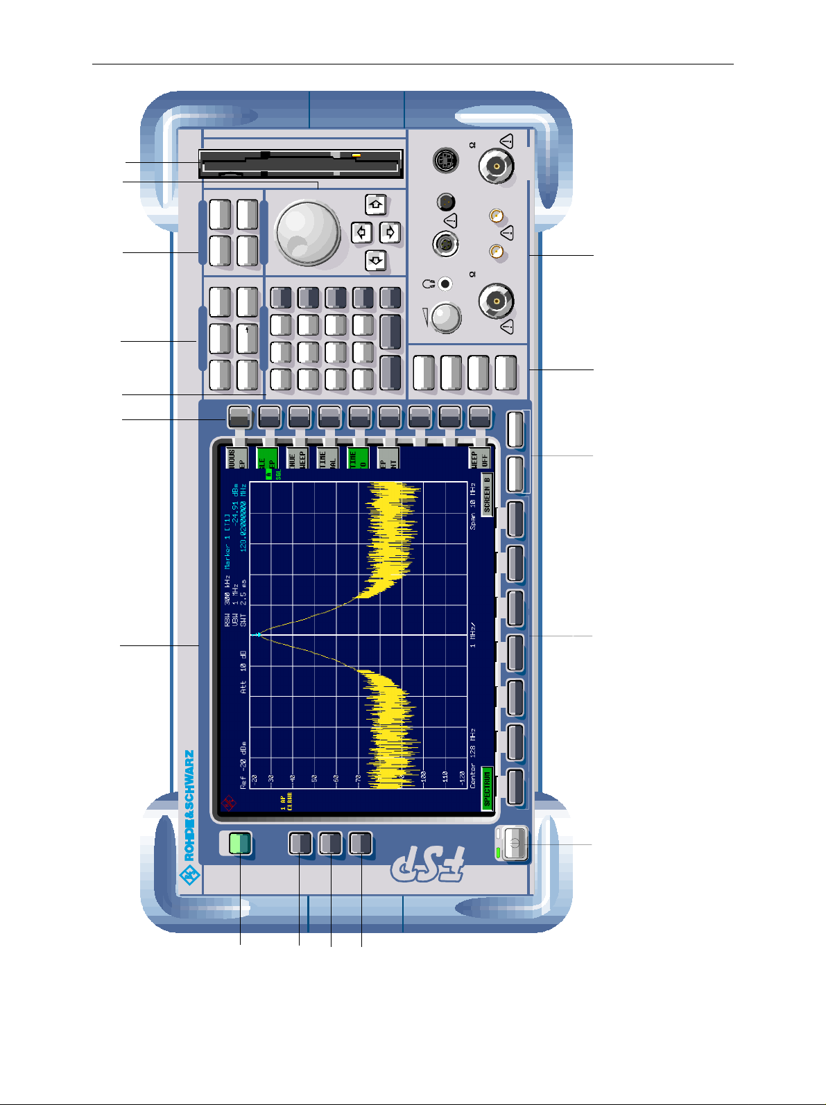
Fig. 1-1 Front View
1164.4556.12 I-1.2 E-1
Page 13
FSP Front View
1 Preparing for Operation
Chapter 1 describes the controls and c onnectors of the Spectrum Analyzer FSP by means of the f ront
and rear view. Then follows all the information that is nec essar y to put the instrument into oper ation and
connect it to the AC supply and to external devices.
A more detailed description of the hardware connectors and interfaces can be found in chapter 8.
Chapter 2 provides an introduction into the operation of the FSP by means of typical examples of
configuration and measurement; for the description of the concept for manual operation and an
overview of menus refer to chapter 3.
For a systematic explanation of all m enus, functions and par ameters and back ground inform ation refer
to the reference part in chapter 4.
For remote control of the FSP refer to the general description of the SCPI c ommands, the ins trument
model, the status reporting system, and command description in chapter 5 and 6.
Description of Front and Rear Panel Views
Front View
1
Display Screen see Chapter 3
2
Softkeys see Chapter 3
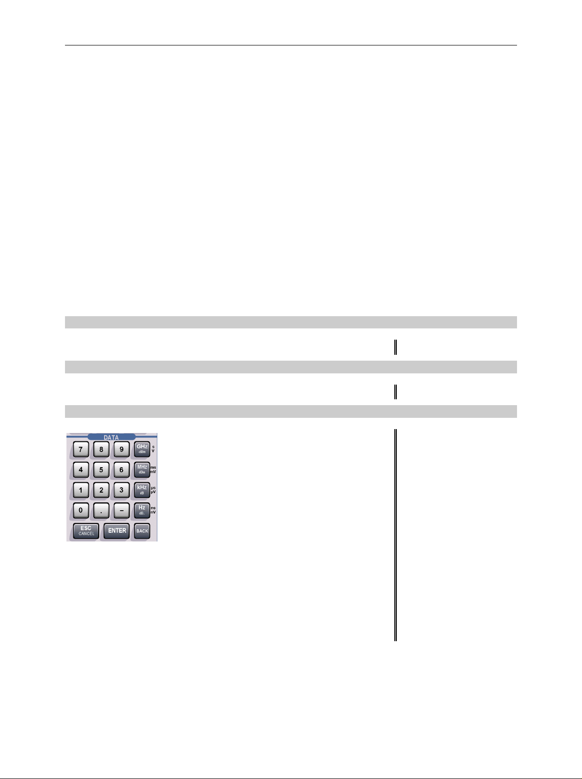
3
data input
0...9 input numbers
see Chapter 3
. input decimal point
– change sign
ESC – close input field (for uncompleted or
CANCEL already closed inputs, the original
entry is kept)
– erase the current entry in input field
(beginning of an input)
– close message window (status, error
and warning messages)
ENTER close the data input.
BACK – erase last character input for
uncompleted input
– restore previous input (undo)
1164.4556.12 1.1 E-1
Page 14

Front View FSP
7
6
5
1164.4391.30
SWEEP
CONTROL
34
2
BW SWEEP
AMPT
SPAN
FREQ
MEAS TRIG
MKR
MKR
MKR
FCTN
VARIATION
s
V
-dBm
GHz
DATA
89
7
µs
µV
ms
mV
dB
dBm
MHz
kHz
3
56
4
12
50
KEYBOARD
PROBE PO WER
ns
nV
dB..
Hz
BACK
-
.
0
AF OUTPUT
ENTER
ESC
CANCEL
TRACE
RF INPUT
EXT MIXER
LO OUT/ IF IN IF I N
GEN OUTPUT 50
DISP
LINES
MADE IN G E RMANY
MAX + 30 d Bm / 0V DC
MAX 0V DC
FILE
PREV NEXT
..
1
11 10 9 8
SPECTRUM ANALYZER 9 kHz ... 30 GHzFSP
CAL
SETUP
14
HCOPY
12
13
PRESET
16
15
Fig. 1-1 Front View
1164.4556.12 1.2 E-1
Page 15
FSP Front View
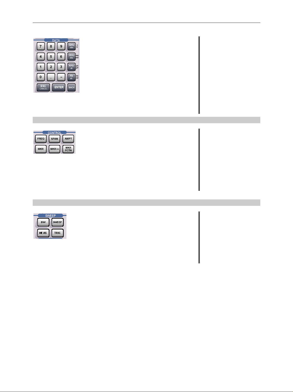
data input
GHz s The units keys close the data
-dBm V input and define the multipli-
cation factor for each basic unit.
MHz ms For dimension-less or
dBm mV alphanumeric inputs, the units
keys have weight 1.
kHz µs They behave, in this case, like the
dB µVENTER key.
Hz ns
dB.. nV
see Chapter 3
4
FREQ Set frequency axis
SPAN Set span
AMPT Set level indication and configure
RF input.
MKR Select and set standard marker and delta
marker functions.
MKR-> Change instrument settings via markers
MKR Select further marker and delta
FCTN marker functions
see Chapter 4
5
BW – Set resolution bandwidth,
video bandwidth and sweep time,
– Set coupling of these
parameters
SWEEP Select sweep
MEAS Select and set power measurements
TRIG Set trigger sources
see Chapter 4
1164.4556.12 1.3 E-1
Page 16

Front View FSP
7
6
5
1164.4391.30
SWEEP
CONTROL
34
2
BW SWEEP
AMPT
SPAN
FREQ
MEAS TRIG
MKR
MKR
MKR
FCTN
VARIATION
s
V
-dBm
GHz
DATA
89
7
µs
µV
ms
mV
dB
dBm
MHz
kHz
3
56
4
12
50
KEYBOARD
PROBE PO WER
ns
nV
dB..
Hz
BACK
-
.
0
AF OUTPUT
ENTER
ESC
CANCEL
TRACE
RF INPUT
EXT MIXER
LO OUT/ IF IN IF I N
GEN OUTPUT 50
DISP
LINES
MADE IN G E RMANY
MAX + 30 d Bm / 0V DC
MAX 0V DC
FILE
PREV NEXT
..
1
11 10 9 8
SPECTRUM ANALYZER 9 kHz ... 30 GHzFSP
CAL
SETUP
14
HCOPY
12
13
PRESET
16
15
Fig. 1-1 Front View
1164.4556.12 1.4 E-1
Page 17
FSP Front View
≥
≥
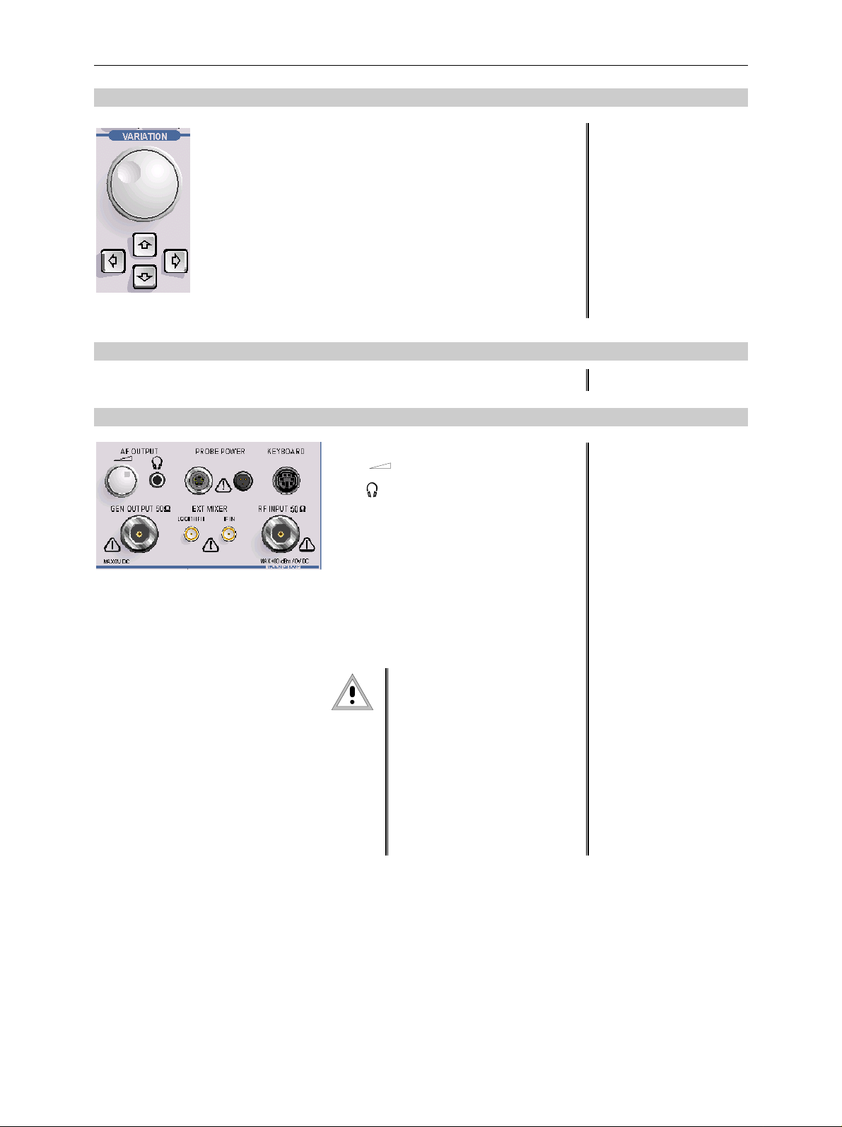
6
Key group for entering data and for cursor movement
Cursor keys – Move the cursor within the input
fields and tables.
– Vary the input value.
– Define the direction of movement
for the roll-key.
Roll-key – Vary input values.
– Move markers and limits.
– Select letters in the help line editor.
– Move cursor in the tables
– Close data input (ENTER)
see Chapter 3
7
3 1/2" diskette drive; 1.44 MByte
8
AF OUTPUT (only with option FSP-B3)
Volume control
Head phone
connector
PROBE POWER Power supply and
coded socket
(+15 V/ -12 V) for
accessories
KEYBOARD Connector for an
external keyboard
see Chapter 8
RF INPUT RF input
Caution:
For FSP3 and FSP7 The
maximum DC voltage is 50 V,
the maximum power is
1 W (=^ 30 dBm) at
attenuation.For FSP13 and
FSP30, the maximum DC
voltage is 0 V, the maximum
power is
1 W ( 30 dBm at
attenuation)
see Chapter 8
10 dB
30 dB
1164.4556.12 1.5 E-1
Page 18
Front View FSP
7
6
5
1164.4391.30
SWEEP
CONTROL
34
2
BW SWEEP
AMPT
SPAN
FREQ
MEAS TRIG
MKR
MKR
MKR
FCTN
VARIATION
s
V
-dBm
GHz
DATA
89
7
µs
µV
ms
mV
dB
dBm
MHz
kHz
3
56
4
12
50
KEYBOARD
PROBE PO WER
ns
nV
dB..
Hz
BACK
-
.
0
AF OUTPUT
ENTER
ESC
CANCEL
TRACE
RF INPUT
EXT MIXER
LO OUT/ IF IN IF I N
GEN OUTPUT 50
DISP
LINES
MADE IN G E RMANY
MAX + 30 d Bm / 0V DC
MAX 0V DC
FILE
PREV NEXT
..
1
11 10 9 8
SPECTRUM ANALYZER 9 kHz ... 30 GHzFSP
CAL
SETUP
14
HCOPY
12
13
PRESET
16
15
Fig. 1-1 Front View
1164.4556.12 1.6 E-1
Page 19
FSP Front View
9
10
11
12
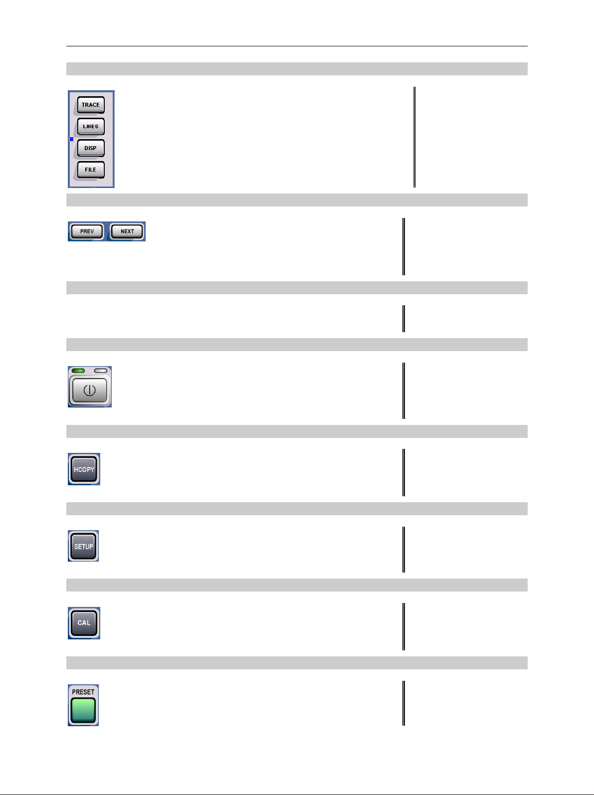
TRACESelect and activate traces and detectors
LINES Set limit lines
DISP Configure display
FILE – Save and recall instrument data
– Configuration of memory media and data
Menu-change keys
NEXT Change to side menu
PREV Call main menu
Hotkeys see Chapter 3
ON/STANDBY switch see Chapter 1
see Chapter 4
see Chapter 3
13
14
15
16
Configure and start a print job see Chapters 1 and 4
Define general configuration see Chapter 4
Record correction data see Chapter 4
Call default settings see Chapter 4
1164.4556.12 1.7 E-1
Page 20

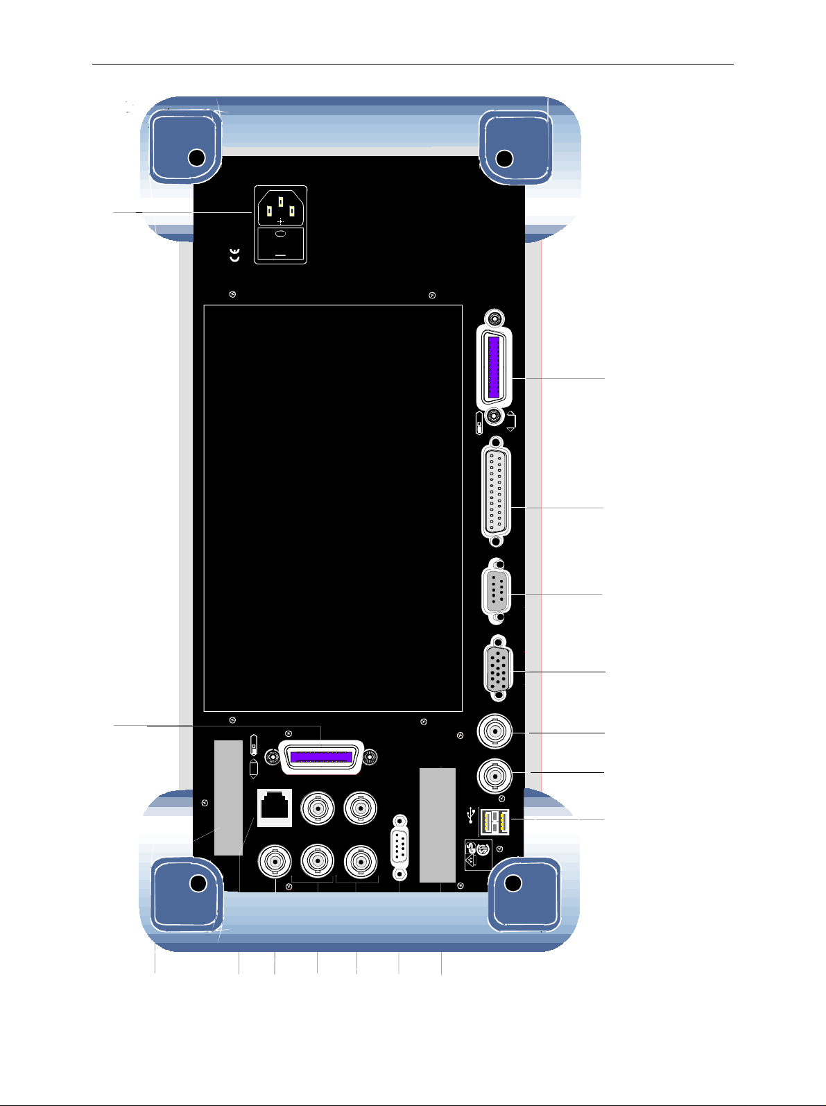
Rear View FSP
18
100 - 240 VA C
3.1 - 1.3 A
19
625
SC PI
17
20
21
MONITOR COM LPT
625
IEC 2
SC PI
SC PI
SC PI
I / Q DATA OUT
SC PI
LAN
20.4 - MHz OUT
TG Q IN
TG I IN
TG Q IN
REF OUT
USER PORT
REF IN
AUX CONTROL
NOISE
SOURC E
NOISE
GATE IN
EXT T RIG /
USB
®
US
C
LR 114 196
22
23
24
25
32
31
30
29
28
27
26
Fig. 1-1 Rear View
1164.4556.12 1.8 E-1
Page 21
FSP Rear View
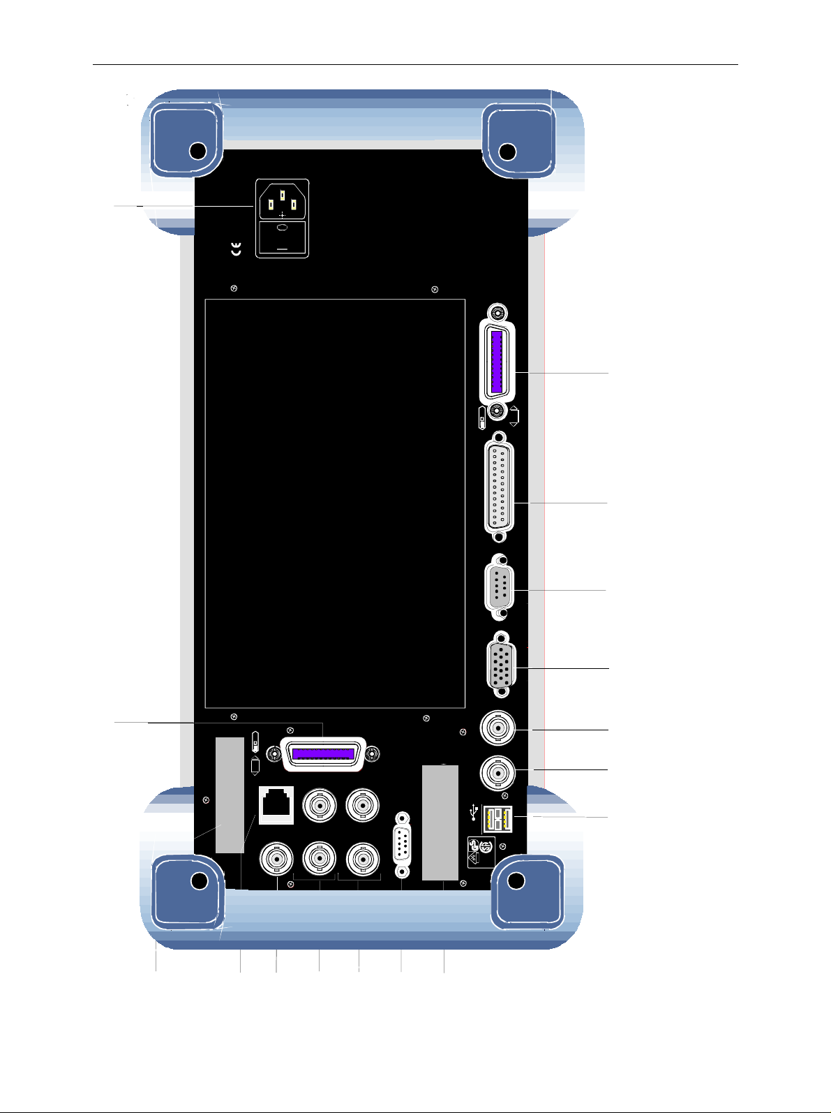
Rear View
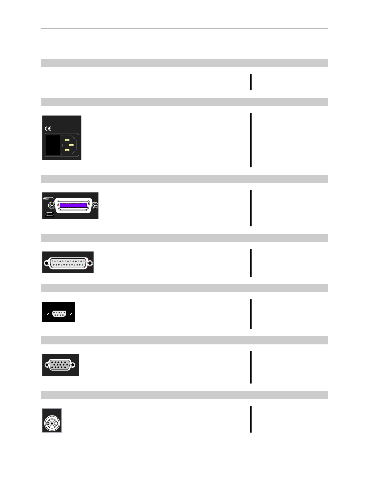
17
Reserved for options see Chapter 8
18
100 - 240 VAC
3.1 - 1.3 A
I 0
19
625
SCPI
20
21
LPT
Power switch and AC power connector see Chapter 1
IEC/IEEE bus-connector see Chapter 8
Parallel interface connector
see Chapter 8
(printer connector)
COM
Connector for a serial interface
see Chapter 8
(9-pin socket; COM)
22
MONITOR
Connector for an external monitor see Chapter 8
23
NOISE
SOURCE
1164.4556.12 1.9 E-1
Output connector for an external noise source see Chapter 8
Page 22
Rear View FSP
18
100 - 240 VA C
3.1 - 1.3 A
19
625
SC PI
17
20
21
MONITOR COM LPT
625
IEC 2
SC PI
SC PI
SC PI
I / Q DATA OUT
SC PI
LAN
20.4 - MHz OUT
TG Q IN
TG I IN
TG Q IN
REF OUT
USER PORT
REF IN
AUX CONTROL
NOISE
SOURC E
NOISE
GATE IN
EXT T RIG /
USB
®
US
C
LR 114 196
22
23
24
25
32
31
30
29
28
27
26
Fig. 1-2 Rear View
1164.4556.12 1.10 E-1
Page 23
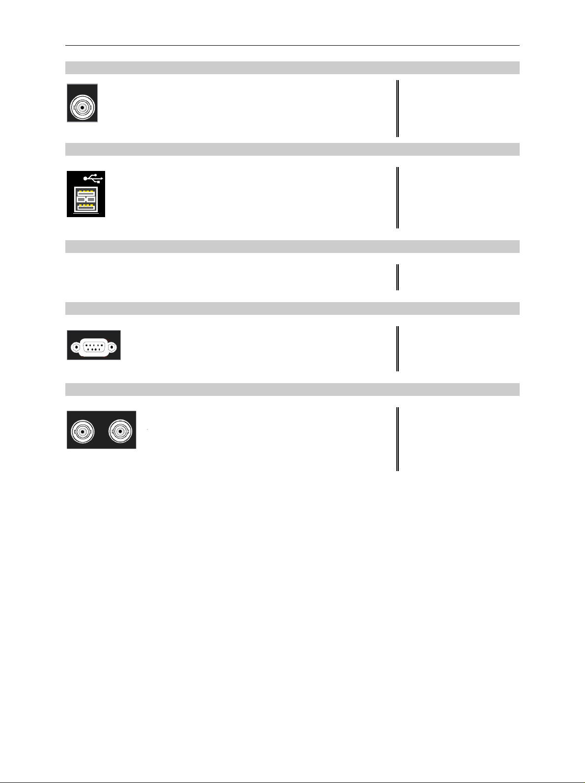
FSP Rear View
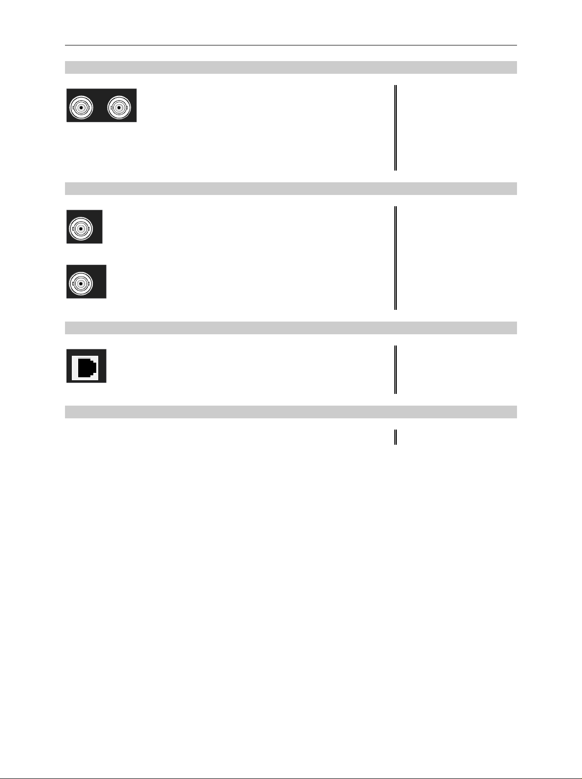
24
EXT TRIG /
GATE IN
25
Input connector for an external trigger or an
external gate signal
see Chapter 8
USB
26
27
AUX CONTROL
28
REF IN REF OUT
Connector for USB see Chapter 8
Reserved for options
Connector to control an external generator ((only
with option FSP-B10)
REF IN Input connector for an external
see Chapter 4
reference (10 MHz)
REF OUT Output connector for an internal
reference (10 MHz)
1164.4556.12 1.11 E-1
Page 24
Rear View FSP
18
100 - 240 VAC
3.1 - 1.3 A
19
625
SC PI
17
20
21
MONITOR COM LPT
625
IEC 2
SCP I
SCP I
SCP I
I / Q DATA OUT
SCP I
LAN
20.4 - MHz OUT
TG Q IN
TG I IN
TG Q IN
REF OUT
USER PORT
REF IN
AUX CONTROL
NOISE
SOURC E
NOISE
GATE IN
EXT TRI G /
USB
®
US
C
LR 114 196
22
23
24
25
32
31
30
29
28
27
26
Bild 1-2 Rear View
1164.4556.12 1.12 E-1
Page 25
FSP Rear View
29
TG I IN TG Q IN
30
20.4 - MHz OUT
CVS IN/OUT
31
LAN
TG IN Signal input connector for external
modulation of Tracking Generator
(option FSP-B9)
TG Q IN Signal input connector for external
modulation of Tracking Generator
(option FSP-B9)
Output connector for 20.4 MHz IF
see Chapter 8
(replaced by CCVS IN OUT if option FSP-B6 is
built in)
Selectable CCVS input/output
see Chapter 4 and 8
(only if option FSP-B6 is built in)
LAN Interface (option FSP-B16) see Chapter 4
32
Reserved for options
1164.4556.12 1.13 E-1
Page 26

Getting Started with the Instrument FSP
Getting Started with the Instrument
The following section describes how to activate the instrument and how to connect external devices
such as printer and monitor.
Chapter 2 explains the operation of the instrument using simple measurement examples.
Important:
Prior to switching on the instrument, make sure that the following conditions are fulfilled:
• The instrument cover is in place and tightly screwed on
• Fan openings are not obstructed
• Signal levels at the inputs are within specified limits
• Signal outputs are connected correctly and not overloaded.
Any non-compliance may cause damage to the instrument .
Preparing the Instrument for Operation
Ø Take the instrument out of the packaging and check whether the
items listed in the pack ing list and in the lists of acces sories are all
included.
Ø Remove the two protective covers from the front and rear of the FSP
and carefully check the instrument for damage.
remove protective caps
Ø Should the instrument be damaged, immediately notify the carrier
and keep the box and packing material.
Ø For further transport or shipm ent of the FSP, the original packing
should be used. It is recommended to keep at least the two
protective covers of the front and rear panels in order to prevent
damage to the controls and connectors.
Setting Up the Instrument
Standalone Operation
The instrument is designed for use under general laboratory conditions. The ambient conditions required
at the site of operation are as follows:
• The am bient tem per ature m ust be in the range spec ified in
Wrist strap with cord
Building ground
Ground connection
of operational site
Heel strap
Floor mat
the data sheet.
• All fan openings must be unobstructed and the air flow at
the rear panel and at the side-panel perforations must be
unimpeded. The distance to the wall should be at least
10 cm.
• The mounting surface should be flat.
• To avoid damage of electronic components of the DUT
due to electrostatic discharge on manual touch, protective
measures against electrostatic discharge are
recommended.
1164.4556.12 1.14 E-1
Page 27
FSP Getting Started with the Instrument
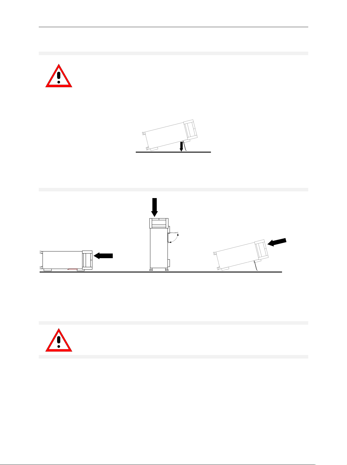
Safety Instruction for Instruments with Tiltable Feet
Warning
The feet must be fully folded in or out. Only in this way can the stability of the
instrument be guaranteed and reliable operation be ensured. W ith the feet out, the
total load for the feet must not exceed 500 N (own weight and additional units put
onto the instrument). These units must be sec ured against slipping (e.g. by locking
the feet of the unit at the top side of the enclosure).
<500N
When shifting the instrument with the feet out, the feet might c ollapse and fold in. To
avoid injuries, the instrument must therefore not be shifted with the feet out.
The instrument can be operated in any position.
Rackmounting
Important:
For rack installation, ensure that the air flow at the s ide-panel per for ations and the air
exhaust at the rear panel are not obstructed.
The instrument may be installed in a 19" rack by using a rack adapter kit (Order No. see data sheet).
The installation instructions are part of the adapter kit.
1164.4556.12 1.15 E-1
Page 28
Getting Started with the Instrument FSP
EMC Safety Precautions
In order to avoid electromagnetic interference (EMI), the instrument may be operated only with all covers
closed. Only adequately shielded signal and control cables may be used (see recommended
accessories).
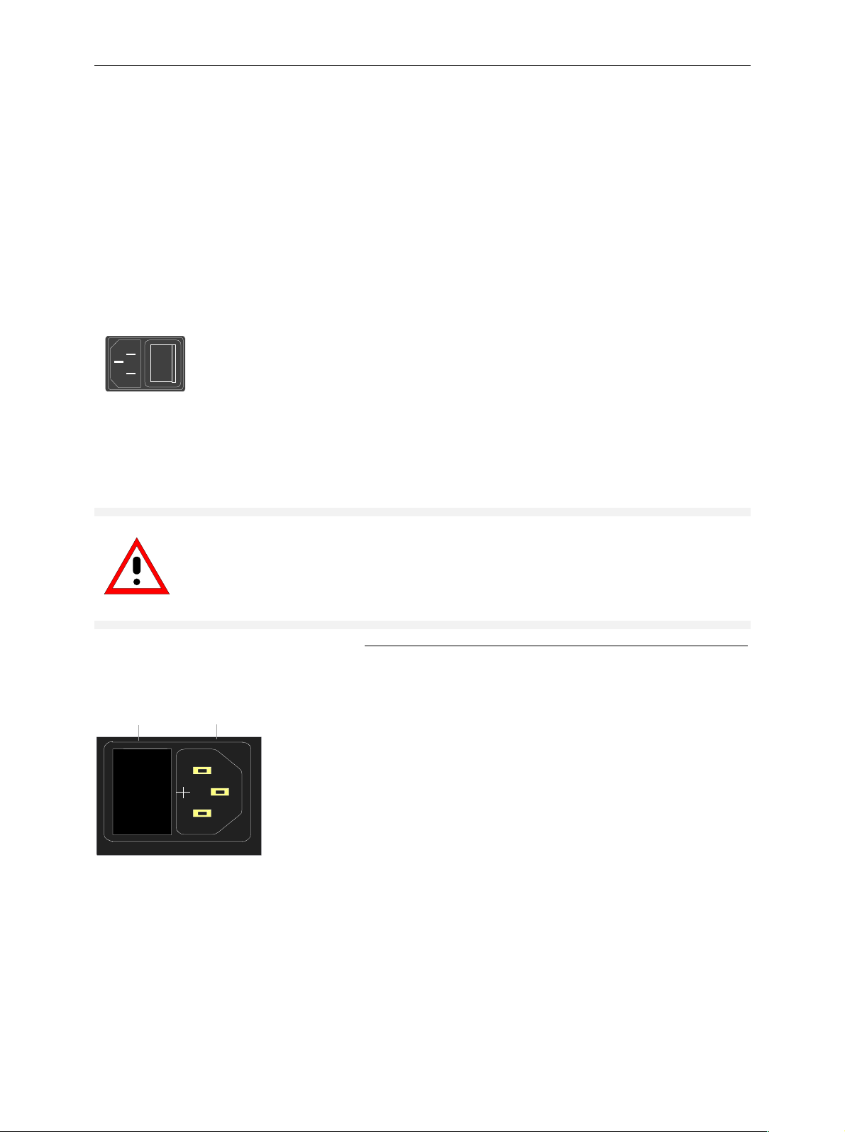
Connecting the Instrument to the AC Supply
The FSP is equipped with an AC voltage selection feature and will automatically adapt itself to the
applied AC voltage (range: 100 to 240 V AC, 40 to 400 Hz). External voltage selection or adaptation of
the fuses are not necessary. The AC power connector is located on the rear panel (see below).
Ø Connect the instrument to the AC power source using the AC
I
o
Power connector
power cable delivered with the instrument.
As the instrument is designed according to the regulations for
safety class EN61010, it must be connected to a power outlet
with earthing contact.
Switching the Instrument On/Off
Caution:
Do not power down during booting. Such a switch-off may lead to corr uption of
the hard disk files.
AC power switch on the rear panel
Power switch
Power connec tor
I 0
Power switch
Position I = ON
In the I position, the instrument is in st andby mode or in
operation, depending on the position of the
ON/STANDBY key at the front of the instrument.
Note:
The AC power switch may remain ON continuously.
Switching to OFF is only required when the instrument
must be completely removed from the AC power source.
Position O = OFF
The 0 position implies an all-pole disconnection of the
instrument from the AC power source.
1164.4556.12 1.16 E-1
Page 29
FSP Getting Started with the Instrument
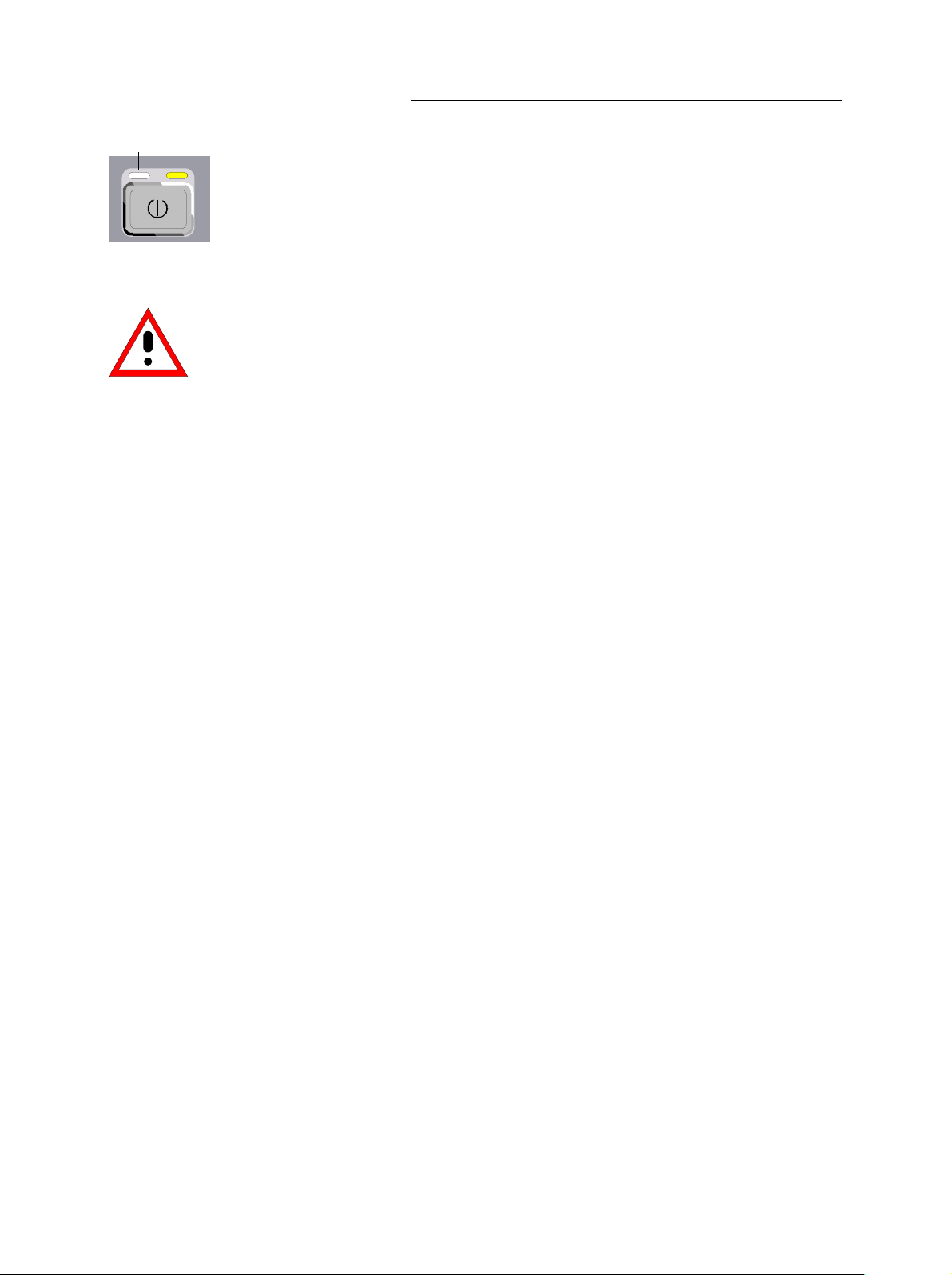
ON/STANDBY switch on the front panel
ON STANDBY
Caution:
In standby mode, the AC
power voltage is present
within the instrument
Standby switch
The ON/STANDBY switch activates two different oper ating
modes indicated by coloured LEDs:
Operation ON - ON/STANDBY is depressed
The green LED (ON) is illuminated. The instrument is
ready for operation. All modules within the instrument are
supplied with power.
STANDBY - ON/STANDBY switch is not pressed.
The yellow LED (STANDBY) is illuminated. Only the
power supply is supplied with power and the quartz oven
is maintained at normal operating temperature.
Switching On the Instrument
Ø In order to switch on the FSP, set the power switch on the rear panel to position I.
Ø Set the F SP to operating mode by pressing the ON/STANDBY key on the front panel. The green
LED must be illuminated.
Startup Menu and Booting
After switching on the instrum ent, a message indicating the ins talled BIOS version (e.g. Analyzer BIOS
Rev. 1.2) appears on the screen for a few seconds.
Subsequently Windows XP is booted fir st and after that the instrument firm ware will boot. As soon as
the boot process is finished the ins trument will start measuring. T he settings used will be the one that
was active when the instrument was previously switched off, provided no other device c onf igur ation than
FACTORY had been selected with STARTUP RECALL in the FILE menu.
Switching Off the FS P
Ø Switch the ON/STANDBY key on the front panel to standby mode by pressing it once.
The yellow LED must be illuminated.
Only when removing the FSP completely from t h e A C p o w e r so u r ce :
Ø Set the power switch at the rear panel to position 0.
1164.4556.12 1.17 E-1
Page 30

Function Test FSP
Power-Save Mode
Display:
The FSP offers the possibility of switching on a power-save mode for the screen display. The
backlighting will be switched off if no entry is made on the front panel (key, softkey or hotkey as well as
spinwheel) during the selected response time.
In order to switch on the power-save mode:
1. Call the DISPLAY - CONFIG DISPLAY submenu to configure the screen display:
Ø Press DISP key
Ø Press CONFIG DISPLAY softkey
2. Activate the save mode
Ø Press DISPLAY PWR SAVE softkey.
The softkey is highlighted in colour, thus indicating that the power-save mode is on. At the
same time the data entry for the delay time is opened.
3. Define the delay time
Ø Enter the required response time in minutes and confirm the entry using the ENTER key.
The screen will be blanked out after the selected time period has elapsed.
A power-save mode is preset f or the built-in hard disk which is automatic ally closed down 15 minutes
after the last access.
Recalling the Most Recent Instrument Settings
The FSP stores its current inst rument settings onto the hard disk every time it is switched of f via the
ON/STANDBY key. After each power-on, the FSP is reloaded with the operational parameters which
were active just prior to the last power-off (STANDBY or AC power OFF) or were set with ST ARTUP
RECALL (see Chapter 4 "Saving and Recalling Data Sets").
Note: Storing the current instrument settings is not possible if the ins trument is s witched off us ing
the POWER ON switch at the rear panel or when unplugging the mains cord. After poweron the instrument settings stored previously on the hard disk will be loaded in this case.
Function Test
After turning on the AC power, the FSP will display the following message on the display screen:
Rohde & Schwarz GmbH & Co. KG
Analyzer BIOS Vx.y
After appearance of the above message, a selftest of the controller hardware is performed.
Subsequently, the Windows NT controller boots and the measurement screen will appear.
The system self- alignment is activated via CAL key, CAL TOTAL softkey. The individual res ults of the
self-alignment (PASSED / FAILED) can be displayed in the CAL menu (CAL RESULTS).
With the aid of the built-in selftest functions (SETUP key, SERVICE, SELFTEST soft keys), the
functional integrity of the instrument can be verified and/or defective modules can be localized.
1164.4556.12 1.18 E-1
Page 31

FSP Windows NT
Windows XP
Caution:
The drivers and programs used under Windows XP are adapted to the measuring
instrument. In order to prevent the instrument functions from damage, the settings
should only be modified as described below.
Existing software may only be modified using update software released by Rohde &
Schwarz.
Additionally only programs authorized by Rohde & Schwarz for use on the FSP may
be run on the instrument.
Do not power down during booting. Such a switch-off may lead to corruption of
the hard disk files.
The instrument runs under the operating system Windows XP Embedded. The com puter c an be used to
install and configure device drivers that were authorized by Rohde & Schwarz. Any further use of the
computer function is only allowed under the conditions described in this operating manual.
Login
Windows XP requires a login process , during which the user is asked for identif ication by entering his
name and password. As a factory default the instrum ent is configured for Auto Login, i.e. the login is
performed automatic ally and in the background. The user name used f or this is "instrument" and the
password is also "instrument" (in small letters).
Administrator level
The NT user account used for the autologin function has administrator access rights.
Windows XP Service Packs
The Windows XP Embedded system installed on the instrument includes Service Pack 1 for XP
Embedded.
Any service pack not approved by Rohde & Schwarz must not be installed since malfunctions
may occur. These malfunctions could impair measurements that are correctly performed on the
instrument and necessitate a repair.
The user is especially warned against using Service Pack s of Windows XP Hom e or of the Pr ofes sional
Edition, since these Service Packs are not compatible with Windows XP Embedded.
Calling the Windows XP start menu
The Windows NT start menu is called using the key combination <CTRL> <ESC>. It is possible to
access the required subm enus f rom the star t m enu by means of the m ouse or the cur sor k eys. In order
to return to the measurement screen the button "R&S Analyzer Interface" in the W indows NT task bar
can be used.
1164.4556.12 1.19 E-1
Page 32

Connecting an External Keyboard FSP
Connecting an External Keyboard
Caution:
Connect the keyboard only when the instrument is switched off
(STANDBY). Otherwise, proper functioning cannot be ens ured due to interactions with
the firmware.
The FSP allows an external PC keyboard to be connected to the 6-pin PS/2 connector labelled
KEYBOARD on the front panel or to the USB interface on the rear panel.
KEYBOARD
USB
The keyboard makes it easier to enter comments, file names, etc, when measurements are performed.
If the keyboard is to be connected to the PS/2 connector, the PSP-Z2 keyboard (Order No.
1091.4100.02, English) is recomm ended. This keyboard includes not only the PC keyboard but also a
trackball for controlling the mouse.
Keyboards and mouse devices in line with the USB standard 1.1 are suitable f or connection to the USB
interface.
The keyboard (except for PSP-Z2, see above) will automatically be recognized after connection. The US
keyboard assignment is the default setting. Special settings such as ref resh rate can be performed in
the Windows XP menu START - SETTINGS - CONTROL PANEL - KEYBOARD.
Chapter 8 contains the interface description for the connectors.
1164.4556.12 1.20 E-1
Page 33

FSP Connecting an External Keyboard
Connecting a Mouse
To make Windows XP operation easier, the allows a mouse to be connected to the PS/2 mouse
interface or to the USB interface on the rear panel.
To make Windows XP operation easier, the F SP allows a mouse to be connec ted to the USB interface
on the rear panel.
USB
Microsoft and Logitech mouse types are supported.
Note. The recommended keyboard PSP-Z2 is equipped with a track ball for mouse c ontr ol. Connecting
an additional mouse will cause interface conflicts and lead to malfunctions of the instrument.
After connection the mouse is automatically recognized. Special settings suc h as mouse cursor s peed
etc, can be performed in the Windows XP menu START - SETTINGS - CONTROL PANEL - MOUSE.
Chapter 8 contains the interface description for the connector.
1164.4556.12 1.21 E-1
Page 34

Connecting an External Monitor FSP
Connecting an External Monitor
Caution:
The monitor may only be connected when the instrument is sw itched off (STANDBY).
Otherwise, the monitor may be damaged.
Do not modify the screen driver (dis play type) and display configuration since this will
severely affect instrument operation.
The instrument is equipped with a rear-panel MONITOR connector for the connection of an external
monitor.
MONITOR
After connecting the external monitor the instrument needs to be rebooted in order to recognize the
monitor. After that the measurement screen is displayed on both the external monitor and the
instrument. Further settings are not necessary.
1164.4556.12 1.22 E-1
Page 35

FSP Connecting a Printer
Connecting a Printer
A printer can be connected while the instrument is running.
The FSP allows two different printer c onfigurations for printing a hardc opy to be created plus s witchover
between these two configurations. The DEVICES table in the HCOPY menu shows the available
selection of installed printers (see section 4.4 "Documentation of Measurement Results").
The interfaces for connecting printers are on the rear panel:
LPT
USB
Chapter 8 contains the interface description for the connectors.
Selecting a Printer
Before a hardcopy can be printed, the printer has to be selected from the "HCOPY" menu.
In the following example, an HP DeskJet 660C printer that was preinstalled for LPT1 is selected as
DEVICE2 for hardcopies of the screen content.
Ø Press the HCOPY key.
The HCOPY menu will open.
HCOPY
DEVICE
SETUP
DEVICE
12
COLORS
DEVICE
12
Ø Press the DEVICE 1/2 softkey.
Device 2 will become the active output
unit.
Note:
If the printer is to be operated as device 1,
this step can be omitted.
1164.4556.12 1.23 E-1
Page 36

Connecting a Printer FSP
DEVICE
SETUP
Ø Press the DEVICE SETUP softkey.
The HARDCOPY SETUP table opens and
displays the selection of output formats.
The current selection "Clipboard" is
highlighted and marked with a dot in the
option button.
Ø Use the cursor key
to move the
selection bar to "Printer" and press
ENTER.
Windows for selecting a printer (Name),
printing to file (Print to File) and selecting
printout orientation (Orientation) are
displayed.
Ø Use the cursor key to set the selection
bar to "Name" and press ENTER .
The list of available printer types appears.
Ø Use the cursor key
/ or the
spinwheel to move the selection bar to the
"HP DeskJet 660C" printer and press
ENTER.
The list closes and the selected printer
appears in the "Name" field.
Note:
If the desired printer is not available in the
selection list, its driver must first be
installed.
For further information, see sections
"Installation of Plug&Play Printers",
"Installation of Non-Plug&Play Printers"
and "Installation of Network Printers".
1164.4556.12 1.24 E-1
Page 37

FSP Connecting a Printer
VARIATION
Ø Press the cursor key or turn the
spinwheel until the "Close" button is
reached.
Further settings can still be made:
"Print to File" redirects printing to a f ile. In
this case, the system prompts you for a file
name when printing is started.
Ø The selection is activated by pressing
ENTER or the spinwheel.
"Orientation" is used to switch between
portrait and landscape format.
Ø To change the selection, open the list by
pressing ENTER and select the desired
orientation with the cursor key
/ . To
close the list, press ENTER again.
The "Close" button is used to complete the
setup.
Ø Press ENTER as soon as the "Close"
button is available.
The dialog closes. Printing will now be
performed according to the selected settings.
PRINT
SCREEN
Start printing
Ø Press the PRINT SCREEN softkey.
A hardcopy of the screen contents will be
printed.
1164.4556.12 1.25 E-1
Page 38

Connecting a Printer FSP
The factory setting for DEVICE 2 is "Clipboard". In this case, the printout will be copied to the
Windows XP clipboard which is supported by most Windows applications. The contents of the
clipboard can be pasted directly into a document via EDIT - PASTE.
Table 1-1 Factory settings for DEVICE 1 and DEVICE 2 in the HCOPY menu shows the factory
settings for the two output devices.
Table 1-1 Factory settings for DEVICE 1 and DEVICE 2 in the HCOPY menu
Setting Selection in
configuration table
Output device DEVICE WINDOWS METAFILE CLIPBOARD
Output PRINT TO FILE YES ---
Orientation ORIENTATION --- ---
Setting for DEVICE 1 Setting for DEVICE 2
Installation of Plug&Play Printers
The installation of Plug&Play printers under Windows XP is quite simple:
After the printer is connected and s witched on, Windows XP autom atically recognizes it and installs its
driver, provided the driver is included in the XP installation.
If the XP printer driver is not f ound, Windows XP prom pts you to enter the path f or the corresponding
installation files. In addition to pre-installed driver s, a number of other printer drivers can be f ound in
directory D:\I386.
Note: When installing new printer dr ivers, you will be prompted to indicate the path of the new
driver. This path may be on a disk in dr ive A. Alternatively, the driver can be loaded via a
memory stick or USB CD-ROM drive (see section "Connection of USB Devices").
Installation of Non-Plug&Play Printers
Note: The dialogs below can be controlled either from the front panel or via the mouse and
keyboard (see sections "Connec ting a Mouse" and "Connecting a Keyboard"). Mouse and
PC keyboard are absolutely essential for configuring network printers.
A new printer is installed with the INSTALL PRINTER softkey in the HCOPY menu.
Ø Press the HCOPY key.
The HCOPY menu will open.
HCOPY
DEVICE
SETUP
DEVICE
12
COLORS
1164.4556.12 1.26 E-1
Page 39

FSP Connecting a Printer
NEXT
INSTALL
PRINTER
Ø Press the NEXT key to open the side
menu.
Ø Press INSTALL PRINTER to open the
Printers and Faxes dialog window.
Ø Select Add Printer in the list using the
spinwheel.
Ø Highlight the selected item with CURSOR
RIGHT and press ENTER or the
spinwheel to confirm the selection.
The Add Printer Wizard is displayed.
Ø Select NEXT with the spinwheel and press
the spinwheel for confirmation.
Local or Network Printer can be selected.
1164.4556.12 1.27 E-1
Page 40

Connecting a Printer FSP
Ø To install a local printer, select Local
printer attached to this computer with the
spinwheel. Press the spinwheel for
confirmation and continue with the "Local
Printer" section.
Ø To install a network printer, select A
network printer or a printer attached to
another computer. Press the spinwheel for
confirmation and continue with the
"Network Printer" section.
Local Printer
In the following example, a Star LC24 printer is connected to the LPT1 interface and configured as
DEVICE2 for hardcopies of screen contents. The Add Printer Wizard has already been opened as
described in the section "Starting the Add Printer Wizard" .
Ø To select the USB interface, open the list
of ports by clicking the spinwheel.
Select the printer port with
spinwheel/arrow keys and confirm by
pressing the spinwheel. The selection lis t
is closed again.
Ø To select the LPT connec tor, the selection
list need not be opened.
Ø Place the cursor on the Next button and
confirm by pressing the spinwheel.
The "Install Printer Software" dialog is
opened.
1164.4556.12 1.28 E-1
Page 41

FSP Connecting a Printer
Ø Select the desired manufac turer ( "Star") in
the Manufacturer table using the up / down
keys.
Ø Go to the Printers list with the spinwheel.
Ø Select the desired printer type (Star LC24-
200 Colour) using the up / down k eys and
confirm with ENTER.
Note:
If the desired printer type is not in the list, the
respective driver is not installed yet. In this
case click the HAVE DISK button with the
mouse key. You will be prompted to ins ert a
disk with the corresponding printer driver.
Press OK and select the desired printer
driver.
Ø The printer name can be changed as
required in the Printer name entry field
(max. 60 characters). A PC keyboard is
required in this case.
Ø Use the spinwheel to select Yes or No for
the default printer.
Ø Choose the desired status with the up
/down keys.
Ø Confirm with ENTER.
The Printer Sharing dialog is opened.
1164.4556.12 1.29 E-1
Page 42

Connecting a Printer FSP
Ø Exit the dialog with ENTER.
The Print Test Page dialog is opened.
Ø Exit the dialog with ENTER.
The Completing the Add Printer Wizard
dialog is opened.
Ø Check the displayed settings and exit the
dialog with ENTER.
The printer is installed. If Windows finds
the required driver files, the installation is
completed without any further queries.
If W indows cannot find the required driver
files, a dialog is opened where the path for
the files can be entered.
1164.4556.12 1.30 E-1
Page 43

FSP Connecting a Printer
Ø Select the Browse button with the
spinwheel and confirm with by pressing
the spinwheel.
The Locate File dialog is opened.
Ø Turn the spinwheel to select the directory
and path D:\I386 and press it to confirm
the selection.
If the selected item is not pr inted on a blue
background, it must be marked with the
cursor up / down keys before it can be
activated by pressing the spinwheel.
Ø Select the driver file with the spinwheel
and confirm by pressing the spinwheel.
The file is included in the Files Needed
dialog.
Note:
If the desired file is not in the D:\I386
directory, a disk with the driver file is
needed. In this case, exit the dialog with
ESC and repeat the selection starting from
the "Files needed" dialog.
1164.4556.12 1.31 E-1
Page 44

Connecting a Printer FSP
Ø Select the OK button with the spinwheel
and press the spinwheel to confirm.
The installation is completed.
Finally, the instrument must be configured for printout with this printer using the softkeys DEVICE
SETUP and DEVICE 1/2 in the hardcopy main menu (see section "Selecting a printer").
1164.4556.12 1.32 E-1
Page 45

FSP Connecting a Printer
Configuring a Network Printer (with Option FSP-B16 only)
Ø To select a network printer, click the option
"A network printer or a printer attached to
another computer".
Continue with Next.
Ø Click Browse for a printer and then Next.
A list of selectable printers is displayed.
Ø Mark the desired printer and select it with
OK.
1164.4556.12 1.33 E-1
Page 46

Connecting a Printer FSP
Ø Confirm the subsequent prom pt to install a
suitable printer driver with "OK".
The list of available printer drivers is
displayed.
The manufacturers are listed in the lefthand table, the available printer drivers in
the right-hand table.
Ø Select the manufacturer from the
Manufacturers table and then the printer
driver from the Printers table.
Note:
If the desired type of output device is not
shown in the list, the driver has not yet been
installed. In this case, click the "HAVE DISK"
button. You will be prompted to insert a disk
with the corresponding printer driver. Insert
the disk, select "OK" and then choose the
desired printer driver.
Ø Click Next.
If one or more printers have already been
installed, this window queries whether the
printer last installed is to be used as the
default printer for the Windows XP
applications. The default selection is No.
Ø Start the printer driver installation with
Finish.
Finally, the instrument has to be configured for printout with this printer using the softkeys DEVICE
SETUP and DEVICE 1/2 in the hardcopy menu (see section "Selection of a Printer").
1164.4556.12 1.34 E-1
Page 47

FSP Connecting an Output Device
Connection of USB Devices
Up to two USB devices can be directly connected to the analyzer via the USB interface on the rear of the
FSP. This number can be increased as required by interconnecting USB hubs.
Owing to the wide variety of available USB devices, the FSP can be expanded with almost no
limitations. The following list shows a selection of USB devices suitable for the FSP:
• Power Sensor R&S NRP-Z11 or R&S NRP-Z21 (Adapter Cable R&S NRP-Z4 required)
• Pendrive (memory stick) for easy data transfer from/to the PC (e.g. firmware updates)
• CD-ROM drive for easy installation of firmware applications
• PC keyboard for entering comments, file names, etc
• Mouse for easy operation of Windows dialogs
• Printer for documentation of measurement results
• Modem for remote control of the FSP over great distances
The installation of USB devices is quite simp le under Windows XP since all USB devic es are Plug&Play.
Apart from the keyboard and the mouse, all USB devices can be connected to or disconnec ted fr om the
FSP while the instrument is running.
After the instrument is connected to the USB interface, Windows XP automatically searches for a
suitable device driver.
If Windows XP does not find a suitable driver, you will be prompted to specify a directory where the
driver software can be found. If the driver software is on a CD, a USB CD-ROM should first be
connected to drive to the FSP.
As soon as the connection between the FSP and the USB device is interrupted, Windows XP will again
recognize the modified hardware configuration and will deactivate the corresponding device driver.
Example:
Connecting a pendrive (memory stick) to the FSP:
1. After the pendrive is connected to the USB interface, Windows XP will recognize the newly
connected hardware:
2. Windows XP installs the corresponding driver.
After successful installation, XP signals that the unit is ready for operation:
3. The pendrive is now available as a new drive and is displayed in Windows Explorer:
1164.4556.12 1.35 E-1
Page 48

Connecting an Output Device FSP
The pendrive can be used as a normal drive to load or save files.
4. If the pendrive is no longer required or if files are to be transferred to another computer, the
pendrive is simply disconnected. Windows XP will then deactivate the driver.
If the corresponding drive is still selected in Explorer, an error message will be displayed indicating
that the drive is no longer available.
1164.4556.12 1.36 E-1
Page 49

FSP Installing Windows NT Software
Installing Windows XP Software
Authorized Windows XP Softw ar e for the Instrument
The driver software and the system s ettings of Windows XP are adapted to the m easurem ent f unctions
of the instrument. Correc t operation of the instrument c an therefore be guaranteed only if the software
and hardware used are authorized or supplied by Rohde & Schwarz.
The following program pac kages have been successfully tested for com patibility with the instrument's
software:
• FS-K3 – software for measuring noise factor and gain
• FS-K4 – software for measuring phase noise
• R&S Power Viewer
(virtual power sensor for displaying the results of Power Sensors NRP-Z11 and -Z21)
• Windows XP remote desktop
• FileShredder – for deleting files from the hard disk
• Symantec Norton AntiVirus – software for protection against viruses
The use of other software or hardware may cause failures in the functions of the FSP.
A current list of the software author ized for use on the FSP c an be obtained fr om your nearest Rohde &
Schwarz agency (see list of addresses).
1164.4556.12 1.37 E-1
Page 50

Page 51

FSP Contents– Getting Started
Contents - Chapter 2 "Getting Started"
2 Getting Started..................................................................................................... 2.1
Level and Frequency Measurements............................................................................................. 2.1
Measurement Example 1 – Measuring Frequency and Level using Markers ........................ 2.1
Measurement Example 2 – Measuring Frequency with the Frequency Counter...................2.3
Measurement of Harmonics............................................................................................................2.5
Measuring Harmonics with Frequency Sweeps....................................................................... 2.7
Measurement Example – Measuring the distance between fundamental wave
and the 2
High-Sensitivity Harmonics Measurements........................................................................... 2.10
Measurement Example ...............................................................................................2.10
Measuring the Spectra of complex Signals ................................................................................2.13
Separating Signals by Selecting an Appropriate Resolution Bandwidth...................................... 2.13
Measurement Example - Resolving two signals with a level of –30 dBm each and a
frequency difference of 30 kHz.................................................................................... 2.14
Intermodulation Measurements.............................................................................................2.17
Measurement Example – Measuring the FSP’s intrinsic intermodulation distance.....2.19
nd
and 3
rd
harmonics of the internal reference signal ................................... 2.7
Measuring Signals in the Vicinity of Noise .................................................................................2.23
Measurement example – Measuring the level of the internal reference generator
at low S/N ratios .......................................................................................................... 2.25
Noise Measurements..................................................................................................................... 2.28
Measuring noise power density.............................................................................................2.28
Measurement example – Measuring the intrinsic noise power density of the
FSP at 1 GHz and calculating the FSP’s noise figure................................................2.28
Measurement of Noise Power within a Transmission Channel.............................................2.31
Measurement Example – Measuring the intrinsic noise of the FSP at 1 GHz in a
1.23 MHz channel bandwidth with the channel power function...................................2.31
Measuring Phase Noise........................................................................................................ 2.35
Measurement Example -
Measuring the phase noise of a signal generator at a carrier offset of 10 kHz..................... 2.35
Measurements on Modulated Signals ......................................................................................... 2.37
Measurements on AM signals ............................................................................................... 2.37
Measurement Example 1 –
Displaying the AF of an AM signal in the time domain................................................2.37
Measurement Example 2 - .................................................................................................
Measuring the modulation depth of an AM carrier in the frequency domain.............. 2.39
Measurements on FM Signals............................................................................................... 2.40
Measurement Example - Displaying the AF of an FM carrier ..................................... 2.40
Measuring Channel Power and Adjacent Channel Power.....................................................2.43
Measurement Example 1 - ACPR measurement on an IS95 CDMA Signal...............2.44
Measurement Example 2 – Measuring the adjacent channel power of an
IS136 TDMA signal .....................................................................................................2.48
Measurement Example 3 - Measuring the Modulation Spectrum
in Burst Mode with the Gated Sweep Function ........................................................... 2.51
Measurement Example 4 - Measuring the Transient Spectrum in Burst Mode
with the Fast ACP function..........................................................................................2.53
Measurement Example 5 - Measuring adjacent channel power of a
W-CDMA uplink signal................................................................................................2.55
1164.4556.12 I-2.1 E-1
Page 52

Contents – Getting Started FSP
Amplitude distribution measurements ................................................................................... 2.58
Measurement Example – Measuring the APD and CCDF of white noise
generated by the FSP..................................................................................................2.58
Time Domain Measurements........................................................................................................2.61
Power measurements............................................................................................................ 2.61
Measurement Example – Measuring the power of a GSM burst
during the switch-on phase .........................................................................................2.61
Power Ramping Measurement for Burst Signals...................................................................2.63
Measurement Example – Measurements on GSM burst edges using a high time
resolution.....................................................................................................................2.63
Measuring the S/N Ratio of Burst Signals .............................................................................2.65
Measurement Example - S/N ratio of a GSM signal ...................................................2.65
1164.4556.12 I-2.2 E-1
Page 53

FSP Level and Frequency Measurements
2 Getting Started
Chapter 2 explains how to operate the FSP using typical measurements as examples. Chapter 3
describes the basic operating steps such as selecting the m enus and setting param eters, and explains
the screen structure and displayed function indicators.
Chapter 4 describes all the menus and FSP functions.
All of the following examples are bas ed on the standard settings of the analyzer. These are set with the
PRESET key. A complete listing of the standard settings can be found in chapter 4, section "Pr eset
settings of the FSP – PRESET key".
Level and Frequency Measurements
Measuring the frequency and level of a signal is one of the m ost common purposes for the use of a
spectrum analyzer. For unknown signals, the spectrum analyzer default settings (PRESET) are a good
starting point for the measurement.
If signal levels at the RF input are expected to be above 30 dBm (= 1 W), a power attenuator must be
connected to the RF input of the spectrum analyzer. Please note that the total powar of all applied
signals must be tak en into account concerning this limit. If a power attenuator is not used, signal levels
above 30 dBm can destroy the RF attenuator or the input mixer.
Measurement Example 1 – Measuring Frequency and Level using
Markers
It is easy to measure the level and frequency of a sinewave carrier with the marker function. At the
marker pos ition, the FSP indicates the s ignal’s am plitude and frequenc y. The accur acy of the fr equency
measurement is determined by the FSP reference frequency, the resolution of the marker frequency
display and the resolution of the screen.
In the example, the frequency of the 128-MHz internal reference generator is displayed using the
marker.
1. Set the spectrum analyzer to its default settings.
Ø Press the PRESET key.
2. Connect the test signal to the RF INPUT on the instrument front panel.
3. Switch on the internal reference generator.
Ø Press the SETUP key.
The SETUP menu opens.
Ø Press the SERVICE softkey.
The SETUP - SERVICE menu opens.
Ø Press the INPUT CAL softkey.
The internal reference generator is turned on.
The FSP’s RF input is turned off.
4. Set the center frequency to 128 MHz.
Ø Press the FREQ key.
Ø The entry field for the center frequency is displayed on the screen.
Ø Enter 128 from the numeric keypad and terminate the entry with the MHz key.
5. Reduce the measurement frequency range (SPAN) to 1 MHz.
1164.4556.12 2.1 E-1
Page 54

Level and Frequency Measurements FSP
Ø Press the SPAN key.
Ø Enter 1 from the numeric keypad and terminate the entry with the MHz key.
Note: If the SPAN is changed, the resolution bandwidth (RES BW), the video bandwidth
(VIDEO BW) and the sweep time (SW EEP TIME) are also set to new values bec ause
they are defined as coupled functions in the standard PRESET settings.
6. Measure the level and frequency using the marker and read off the results from the screen.
Ø Press the MKR key.
The marker is switched on and automatically jumps to the trace peak.
Note: When a mark er is switched on for the first time, it automatically per forms the PEAK
SEARCH function (as in this example).
If a marker is already active, the PEAK softkey in the MKR-> menu must be pressed in
order to set the currently active marker onto the displayed signal maximum.
The level and frequency indicated by the marker are displayed in the marker info field at the upper
edge of the screen. These are the measurement results.
The info-field header indicates the number of the marker (MARKER 1) and the number of the
trace on which the marker is positioned ([T1] = Trace 1).
Increasing the Frequency Resolution During a Frequency Measurement with a Marker
The frequency resolution of the marker is determined by the pixel resolution of the trace. The FSP uses
501 pixels for a trace, i.e. at a frequency span of 1 MHz each pixel corresponds to a frequency range of
approx. 2 kHz. This gives a maximum error of 1 kHz.
To increase the pixel resolution of the trace, the frequency span has to be reduced.
7. Reduce the frequency span to 10 kHz.
Ø Press the SPAN key.
Ø Enter 10 from the numeric keypad and terminate the entry with the kHz key.
Note: If the SPAN is changed, the resolution bandwidth (RES BW), the video bandwidth
(VIDEO BW) and the sweep time (SW EEP TIME) are also set to new values bec ause
they are defined as coupled functions in the standard PRESET settings.
The internal reference signal is measured with a span of 10 kHz. The pixel resolution of the trace
is now approx. 20 Hz (10 kHz span / 501 pixel), i.e. the accuracy of the marker frequency display
is increased to approx. 10 Hz.
8. Switch on the RF input again for normal operation of the analyzer.
Ø Press the PRESET key or press the SETUP key and the SERVICE softkey.
Ø Press the INPUT RF softkey.
The internal signal path of the FSP is switched back to the RF input in order to resume normal
operation.
1164.4556.12 2.2 E-1
Page 55

FSP Level and Frequency Measurements
Measurement Example 2 – Measuring Frequency with the Frequency
Counter
With the internal frequency counter, frequencies can be measured more accurately than with the
marker. The fr equenc y sweep is stopped at the marker position and the FSP measures the f requenc y of
the corresponding signal. If an analog bandwidth (≥300 kHz) is used, the frequency is measured by
counting the zero-crossings of the last IF . With digital resolution bandwidths (10 Hz to 100 kHz), the
frequency measurement is performed in the IQ baseband by a special approximation algorithm.
The resolution range for the frequency measurement is 0.1 Hz to 10 kHz. At bandwidths ≥300 k Hz, the
time required for the FSP to perform the f requency measurem ent is dependent on the selected counter
resolution (1/(frequency resolution in Hz)). The digital frequency approximation takes about 30 ms to
perform a frequency measurement irrespective of the selected resolution.
The frequency measurement accuracy is determined by the reference frequency of the FSP and the
selected counter resolution.
In the example, the frequency of the 128-MHz internal reference generator is displayed with the marker.
1. Set the spectrum analyzer to the default settings.
Ø Press the PRESET key.
The FSP is in its default state.
2. Switch on internal reference generator
Ø Press the SETUP key.
Ø Press the softkeys SERVICE - INPUT CAL.
The internal 128 MHz reference generator is now on. The FSP’s RF input is turned off.
3. Set the center frequency and the frequency span
Ø Press the FREQ key and enter 128 MHz.
The FSP center frequency is set to 128 MHz.
Ø Press the SPAN softkey and enter 1 MHz.
The FSP frequency span is set to 1 MHz.
4. Switch on the marker
Ø Press the MKR key.
The marker is switched on and set to the signal maximum. The level and the frequency at the
marker are displayed in the marker-info field.
5. Switch on the frequency counter.
Ø Press the SIGNAL COUNT softkey in the marker menu.
The frequency count is displayed in the marker field at the top of the screen along with the set
resolution (1 kHz is the default setting ).
The sweep stops at the marker position and the FSP measures the frequency of the
corresponding signal. The frequency is output in the marker info field. To distinguish the signal
count result from the normal marker frequency display, the marker is labeled with CNT.
1164.4556.12 2.3 E-1
Page 56

Level and Frequency Measurements FSP
6. Set the resolution of the frequency counter to 1 Hz.
Ø Press the NEXT key.
Ø Press the CNT RESOL 1 Hz softkey.
Fig. 2-1 Frequency measurement with a frequency counter
Note: The frequency measurement with the integral frequency counter only gives correct
results for RF sinewaves or discrete spectral lines. To meet the specified
measurement accuracy, the marker should be more than 25 dB above noise.
7. Switch on the RF input again for normal operation of the analyzer.
Ø Press the PRESET key or press the SETUP key and the SERVICE softkey.
Ø Press the INPUT RF softkey.
The internal signal path of the FSP is switched back to the RF input in order to resume normal
operation.
Hint: For bandwidths between 300 kHz and 10 MHz, the FSP uses a frequenc y counter at an IF
of 20.4 MHz. The time for m easuring the frequency is, therefore, inversely proportional to
the selected resolution, i.e. at a resolution of 1 Hz a gate tim e of 1 s econd is r equired f or the
counter. For digital bandwidths below 300 kHz, the frequency is measured in the baseband
by digital frequency approximation. The time required for measuring the frequency is
approx. 30 ms irrespective of the selected resolution.
When measuring the frequency of a sinewave carrier at a high resolution it is , ther ef ore, best
to set a resolution bandwidth of 100 kHz or less. The measurement time will then be
reduced to a minimum.
1164.4556.12 2.4 E-1
Page 57

FSP Measurement of Harmonics
Measurement of Harmonics
Measuring the harmonics of a s ignal is a frequent problem which can be solved best by means of a
spectrum analyzer. In general, every signal contains harmonics which ar e larger than other s. Harmonics
are particularly critical regarding high-power transmitters s uch as trans ceivers bec ause large harm onics
can interfere with other radio services.
Harmonics are produced by nonlinear characteristics. They can often be reduced by lowpass filters.
Since the spectrum analyzer has a nonlinear characteristic, e.g. in its first mixer, measures must be
taken to ensure that harmonics produced in the analyzer do not cause spurious results. If necessary, the
fundamental wave must be selectively attenuated with respect to the other harm onics with a highpass
filter.
When harm onics are being measured, the obtainable dynamic range depends on the K2 intercept of
the spectrum analyzer. The K2 intercept is the virtual input level at the RF input mixer at which the level
of the 2nd harmonic becomes equal to the level of the fundamental wave. In prac tice, however, applying
a level of this magnitude would damage the mixer. Nevertheless the available dynamic range for
measuring the harmonic distance of a DUT can be calculated relatively easily using the second
harmonic intercept.
nd
As shown in Fig. 2-2, the level of the 2
wave is reduced by 10 dB.
Level display
/ dBm
50
40
30
harmonic is reduced by 20 dB if the level of the f undamental
Second
intercep t point
/dBm
10
0
-10
-20
-30
-40
-50
-60
-70
-80
1st harmonic
1
1
-30
-20 0-10 10 20 30 40 50
2nd harmonic
2
1
RF level
/ dBm
Fig. 2-2 Extrapolation of the 1st and 2nd harmonics to the second harmonic intercept at 40 dBm
The following formula f or the obtainable harmonic distortion d
in dB is derived from the straight-line
2
equations and the given intercept point:
= S.H.I – P
d
2
d
P
I
2
= harmonic distortion
= mixer level/dBm
I
S.H.I. = second harmoni c intercept
Note: The mixer level is the applied RF level minus the set RF attenuation.
The formula for the internally generated level P1 at the 2nd harmonic in dBm is:
(1)
= 2 PI – S.H.I. (2)
P
1
The lower measurement limit for the harm onic is the noise floor of the spectrum analyzer. The harmonic
of the measured DUT should – if sufficiently averaged by means of a video filter – be at least 4 dB
above the noise floor so that the measurement error due to the input noise is less than 1 dB.
1164.4556.12 2.5 E-1
Page 58

Measurement of Harmonics FSP
The following rules for measuring high harmonic ratios can be derived:
1. Select the smallest possible IF bandwidth for a minimal noise floor.
2. Select an RF attenuation which is high enough to just measure the harmonic ratio.
The maxim um harm onic distortion is obtained if the level of the harm onic equals the intrins ic noise level
of the receiver. The level applied to the mixer, according to (2), is:
+
noise
=
P
I
2
At a resolution bandwidth of 10 Hz (noise level -143 dBm, S.H.I. = 40 dBm) , this level is –51.5 dBm.
According to (1) a maximum measurable harm onic dis tor tion of 91.5 dB minus a minimum S/N ratio of 4
dB is obtained.
Hint: If the harm onic emerges from noise suf ficiently (approx. >15 dB), it is easy to check (by
changing the RF attenuation) whether the harmonics originate from the DUT or are
generated internally by the spectrum analyzer. If a harmonic originates from the DUT , its
level remains constant if the RF attenuation is increased by 10 dB. Only the displayed noise
is increased by 10 dB due to the additional attenuation. If the harmonic is exclusively
generated by the spectrum analyzer, the level of the harmonic is reduced by 20 dB or is lost
in noise. If both – the DUT and the spectrum analyzer – contribute to the harmonic, the
reduction in the harmonic level is correspondingly smaller.
2/ IPdBmP
1164.4556.12 2.6 E-1
Page 59

FSP Measurement of Harmonics
Measuring Harmonics with Frequency Sweeps
There are advantages in perform ing harmonic m easurements with a single frequency sweep, provided
that the harmonic distance is in a way that a resolution bandwidth can be s elected which is wide enough
to give an acceptably short sweep time.
Measurement Example – Measuring the distance between fundamental wave
and the 2nd and 3
rd
harmonics of the internal
reference signal
1. Set the spectrum analyzer to the default settings.
Ø Press the PRESET key.
The FSP is in its default state.
2. Switch on the internal reference generator
Ø Press the SETUP key.
Press the softkeys SERVICE - INPUT CAL.
The internal 128 MHz reference generator is now on. The FSP’s RF input is switched off.
3. Set the start frequency to 100 MHz and the stop frequency to 400 MHz
Ø Press the FREQ key.
Ø Press the START softkey and enter 100 MHz.
Ø Press the STOP softkey and enter 400 MHz.
The FSP displays the fundamental and the 2
4. Set the RF attenuation to 0 dB to obtain maximum sensitivity
Ø Press the AMPT key.
Ø Press the RF ATTEN MANUAL softkey and enter 0 dB.
nd
and 3rd harmonics of the input signal.
5. Reduce the video bandwidth to average (suppress) noise.
Ø Press the BW key.
Ø Press the COUPLING RATIO softkey.
Ø Select RBW/VBW NOISE [10
The video bandwidth (VBW) will now always be set to a value which is 10 times smaller than the
resolution bandwidth (RBW).
6. Switch on the marker
Ø Press the MKR key.
Marker 1 is switched on and is positioned on the signal maximum (fundamental wave at 128
MHz). The level and the frequency of the marker are displayed in the marker info field.
] using the cursor keys.
1164.4556.12 2.7 E-1
Page 60

Measurement of Harmonics FSP
7. Switch on the delta marker and measure the harmonic distance
Ø Press the MARKER 2 softkey in the marker menu.
Marker 2 is activated as a delta marker (Delta 2 [T1]). It appears automatically on the largest
harmonic of the signal. The frequency and level, related to marker 1, are indicated in the marker
field at the top of the screen.
Ø Press the MARKER 3 softkey in the marker menu.
Marker 3 is activated as a delta marker (Delta 3 [T1]). It appears automatically on the next largest
harmonic of the signal. The frequency and level, related to marker 1 on the fundamental wave,
are displayed in the marker info field at the top of the screen (see Fig. 2-3).
Fig. 2-3 Measuring the harmonic distance of the internal reference generator. Delta marker 2
[T1] and Delta marker 3 [T1] indicate the distance between the fundamental wave
and the 2
nd
and 3rd harmonics.
In order to make the harmonics grow out of the noise, the following things can be done:
• Reducing the video bandwidth
• Averaging the trace
• Reducing the resolution bandwidth
The noise of the analyzer or the DUT (depending on which one is higher) is suppressed by
reducing the video bandwidth and by averaging the trace. Especially for low S/N ratios, the
measurement uncertainty is reduced using the two averaging methods since the s ignal under test
is also freed from noise.
8. Reduce noise by reducing the vide o bandwidth
Ø Press the BW key.
Ø Press the VIDEO BW MANUAL softkey.
Ø Reduce the video bandwidth, e.g. to 10 kHz, using the spinwheel (turn knob counterclockwise),
or enter 10 kHz.
1164.4556.12 2.8 E-1
Page 61

FSP Measurement of Harmonics
The noise is clearly smoothed and the sweep tim e is increased to 25 ms, i.e. the measurem ent
lasts longer. The displayed video bandwidth is marked with an asterisk (*VBW) to indicate that it
is no longer coupled to the resolution bandwidth (see Fig. 2-4).
Fig. 2-4 Suppression of noise during harmonic measurement by reducing video bandwidth
9. Coupling the video bandwidth to the resolution bandwidth again.
Ø Press the VIDEO BW AUTO softkey.
10. Reduce noise by averaging the trace
Ø Press the TRACE key.
Ø Press the AVERAGE softkey.
The noise component of the trace is smoothed by averaging 10 consecutive traces.
Fig. 2-5 Suppression of noise during harmonic measurements by averaging the trace
11. Switch off trace averaging again.
Ø Press the CLEAR/WRITE softkey.
1164.4556.12 2.9 E-1
Page 62

Measurement of Harmonics FSP
12. Reduce noise by reducing the measurement bandwidth.
If the resolution bandwidth is decreased, noise is reduced proportionally, i.e. if the resolution
bandwidth is reduced by a factor of 10, the noise is also reduced by the same factor (corresponds to
10 dB). The amplitude of a sinusoidal signal is not changed by reducing the resolution bandwidth.
13. Set the resolution bandwidth to 10 kHz.
Ø Press the BW key.
Ø Press the RES BW MANUAL softkey and enter 10 kHz.
The noise is reduced by approx. 25 dB compared to the previous setting. Since the video
bandwidth is coupled to the resolution bandwidth, it is reduced to 1 kHz – the same proportional
reduction as the resolution bandwidth. The sweep time is therefore increased to 60 seconds.
14. Reset the resolution bandwidth again (coupling to span).
Ø Press the RES BW AUTO softkey.
If you want to stop the harmonics measurement on the internal reference generator at this point,
switch the FSP’s RF input on again with the following key sequence.
Ø Press the SETUP key and the softkey sequence SERVICE - INPUT RF or press the PRESET
key.
High-Sensitivity Harmonics Measurements
If harmonics have very small levels, the resolution bandwidth required to measure them must be
reduced considerably. The sweep time is, therefore, also increased considerably. In this case, the
measurement of individual har monics is carried out with the spectrum analyzer set to a small span. Only
the frequency range around the harmonics will then be measured with a small resolution bandwidth.
Measurement Example
1. Set the spectrum analyzer to its default settings.
Ø Press the PRESET key.
The FSP is in its default state.
2. Switch on the internal reference generator.
Ø Press the SETUP key.
Ø Press the softkeys SERVICE - INPUT CAL.
The internal 128 MHz reference generator is now on. The FSP’s RF input is switched off.
3. Set the center frequency to 128 MHz and the span to 100 kHz.
Ø Press the FREQ key.
The frequency menu opens.
Ø Enter 128 in the entry field from the numeric keypad and terminate with the MHz key.
Ø Press the SPAN key.
Ø Enter 100 in the entry filed from the numeric keypad and terminate with the kHz key.
The FSP displays the reference signal with a span of 100 kHz and resolution bandwidth of 3 kHz.
1164.4556.12 2.10 E-1
Page 63

FSP Measurement of Harmonics
4. Switching on the marker.
Ø Press the MKR key.
The marker is positioned on the trace maximum.
5. Set the measured signal frequency and the measured level as reference values
Ø Press the REFERENCE FIXED softkey.
Ø The position of the marker becomes the reference point. The reference point level is indicated by
a horizontal line, the reference point frequency with a vertical line. At the same time, the delta 2
marker is switched on at the marker position.
Fig. 2-6 Fundamental wave and the frequency and level reference point
6. Make the step size for the center frequency equal to the signal frequency
Ø Press the FREQ key.
The frequency menu opens.
Ø Press the CF STEPSIZE softkey and press the
=MARKER softkey in the submenu.
The step size for the center frequency is now equal to the marker frequency.
7. Set the center frequency to the 2nd harmonic of the signal
Ø Press the FREQ key.
The frequency menu open. s
Ø Press the up cursor key (below the spinwheel) once.
The FSP’s center frequency is set to the 2
nd
harmonic.
8. Place the delta marker on the 2nd harmonic.
→
Ø Press the MKR
Ø Press the PEAK softkey.
The delta marker jumps to the maximum of the 2
key.
nd
harmonic. The displayed level result is
relative to the reference point level (= fundamental wave level).
1164.4556.12 2.11 E-1
Page 64

Measurement of Harmonics FSP
Fig. 2-7 Measuring the level difference between the fundamental wave (= reference point
level) and the 2
nd
harmonic
The other harmonics are measured with steps 6 and 7, the center frequency being incremented or
decremented in steps of 128 MHz using the up or down cursor key.
1164.4556.12 2.12 E-1
Page 65

FSP Measuring the Spectra of complex Signals
Measuring the Spectra of complex Signals
Separating Signals by Selecting an Appropriate Resolution Bandwidth
One basic characteristic s of the spectrum analyzer is that it can separate the spectral com ponents of a
composite signal. The resolution with which the individual components ar e separated is determined by
the resolution bandwidth. If the resolution bandwidth is too large, spectral c omponents may no longer be
distinct, i.e. they are displayed as a single component.
An RF sinewave signal is displayed on the screen of the spectrum analyzer with the passband
characteristics of the set resolution filter (RBW). It is the 3 dB bandwidth of the filter that is displayed.
Two signals with the same am plitude c an be res olved if the r es olution bandwidth is les s than or equal to
the signals’ frequency difference. If the resolution bandwidth and the frequency difference are equal, a 3
dB level dip can be seen in the middle between the two signals. The sm aller the resolution bandwidth,
the deeper the level dip and the better the signal resolution.
If there are large level differences between signals, the resolution is determ ined by selectivity as well as
by the resolution bandwidth that has been selected. The measure of selectivity used for spectrum
analyzers is the ratio of the 60 dB bandwidth to the 3 dB bandwidth (= shape factor).
For the FSP, the shape factor for bandwidths up to 100 kHz is < 5 and for larger bandwidths < 15, i.e.
the 60 dB bandwidth of the 30 kHz filter is < 150 kHz and that of the 300 kHz filter is < 4.5 MHz.
Although the 3 dB bandwidths only differ by a factor of 10, the 60 dB bandwidths differ by a factor of 30.
The higher spectral resolution with sm aller bandwidths has to be traded off agains t longer sweep tim es
for the same span. T he sweep tim e required to allow the resolution filter s to settle dur ing a s weep at all
signal levels and frequencies to be displayed is given by the following formula.
Span/RBWkSWT •=
SWT = max. sweep time f or correct measurement
k = factor depending on type of resolution filter
= 2.5 for analog IF filter (≥300 k Hz)
= 1 for digital IF filters (≤ 100 kHz)
Span = frequenc y display range
RBW = resolution bandwidth
2
(1)
If the resolution bandwidth is reduced by a factor of 3, the sweep time is increased by a factor of 9.
Note: The impact of the video bandwidth on the sw eep time is not tak en into ac count in ( 1). For the
formula to be valid, the video bandwidth must be ≥ 3 x the resolution bandwidth.
For bandwidths > 300 kHz, the FSP uses 4pole, single-section filters. They require a k f actor of 2.5 to
settle during the frequency sweep. Digital filters with a Gaussian characteristic are used below a
bandwidth of 300 kHz (up to 100 kHz). These filters settle at a k fac tor of 1, i.e. the sweep tim e is 2.5
times shorter than with conventional 4 or 5 pole, single-section filters.
FFT filters can be us ed for resolution bandwidths up to 30 kHz. Like digital filters, they have a shape
factor of less than 5 up to 30 k Hz. For FFT filters, however, the s weep time is given by the following
formula:
SWT = k
span/RBW (2)
i.e. if the resolution bandwidth is reduced by a factor of 3, the sweep time is increased by a factor of 3
only
1164.4556.12 2.13 E-1
Page 66

Measuring the Spectra of complex Signals FSP
Measurement Example - Resolving two signals with a level of –30 dBm each and
a frequency difference of 30 kHz
Example:
Signal
generator 1
Combiner FSP
Signal
generator 2
Fig. 2-8 Test setup for generating two signals
Signal generator settings ( e.g. SMIQ):
Level Frequency
Signal generator 1 -30 dBm 100.00 MHz
Signal generator 2 -30 dBm 100.03 MHz
FSP measurement sequence:
1. Set the spectrum analyzer to its default settings.
Ø Press the PRESET key.
The FSP is in its default state.
2. Set the center frequency to 100.015 MHz and the frequency span to 300 kHz.
Ø Press the FREQ key and enter 100.015 MHz.
Ø Press the SPAN key and enter 300 kHz.
3. Set the resolution bandwidth is to 30 kHz and the video bandwidth to 1 kHz.
Ø Press the BW key.
Ø Press the RES BW MANUAL softkey and enter 30 kHz.
Ø Press the VIDEO BW MANUAL softkey and enter 1 kHz.
Ø The two signals are clearly separated by a 3 dB level dip in the middle of the screen.
Note: The video bandwidth is set to 1 kHz to clearly display the level dip in the middle
between the two signals. At larger video bandwidths, the video voltage which arises
from envelope detection is not suff iciently suppressed. Therefore, additional voltages
occur between the two signals and can be seen on the trace.
1164.4556.12 2.14 E-1
Page 67

FSP Measuring the Spectra of complex Signals
Fig. 2-9 Measurement of two RF sinewave signals with the same level using a resolution
bandwidth which corresponds to the frequency difference of the signals.
Note: The level dip is only exactly in the middle of the screen if the generator frequencies
exactly correspond with the frequenc y display of FSP. To ensure this, the gener ators
and the FSP must have their frequencies synchronized.
4. Set the resolution bandwidth to 100 kHz.
Ø Press the RES BW MANUAL softkey and enter 100 kHz.
The two generator signals can no longer be clearly distinguished.
Fig. 2-10 Measurement on two RF sinewave signals with the same level using a resolution
bandwidth which is greater than their frequency difference.
The resolution bandwidth (RBW) can be reduced again by turning the spinwheel counterclockwise
to obtain a higher frequency resolution.
1164.4556.12 2.15 E-1
Page 68

Measuring the Spectra of complex Signals FSP
5. Set the resolution bandwidth to 1 kHz.
Ø Turn the spinwheel counterclockwise until a bandwidth of 1 kHz is displayed.
The two generator signals are displayed at high resolution. The sweep time increases
considerably (600 ms) because it increases by 1/ RBW
resolution bandwidths (10 dB per bandwidth factor of 10).
2.
The noise floor also goes down at small
Fig. 2-11 Measurement on two RF sinewave signals with the same level using a resolution
bandwidth (1 kHz) which is far below their frequency difference.
6. Switch on the FFT bandwidths.
Ø Set the FILTER softkey to FFT.
IF filtering is now carried out with the FFT algorithm. The sweep time is considerably reduced
from 600 ms to 15 ms (factor of 40). The update rate of the display is increased in almost the
same proportion.
Fig. 2-12 Measurement with FFT filters gives a considerably shorter sweep time and a higher
refresh rate.
1164.4556.12 2.16 E-1
Page 69

FSP Measuring the Spectra of complex Signals
Intermodulation Measurements
If several signals are applied to a DUT with non-linear c haracteristics, unwanted mixing products are
generated – mostly by active components such as am plifiers or mixers. The products created by 3
order intermodulation are partic ularly troublesome as they have frequencies close to the useful signals
and, compared with other products, are c losest in level to the usef ul signals. T he fundam ental wave of
one signal is mixed with the 2
s1 = 2 f u1 – f u2 (1)
f
s2 = 2 f u2 - f u1 (2)
f
where f
s1 and fs2 are the frequencies of the interm odulation produc ts and f u1 and fu2 the f requencies of
nd
harmonic of the other signal.
the useful signals.
The following diagram shows the position of the intermodulation products in the frequency domain.
Level
P
u1
u2
P
a
D3
rd
P
s1
∆
∆
f
f
s1
f
u1
f
f
u2
P
s2
∆
f
f
s2
Frequency
Fig. 2-13 3rd order intermodulation products
Example:
f u1 = 100 MHz, f u2 = 100.03 MHz
s1 = 2 f u1 - f u2 = 2 100 MHz – 100.03 MHz = 99.97 MHz
f
fs2 = 2
f u2 - f u1 = 2 100.03 MHz – 100 MHz = 100.06 MHz
The level of the intermodulation pr oducts depends on the level of the useful signals. If the level of the
two useful signals is increased by 1 dB, the level of the intermodulation products is increased by 3 dB.
The intermodulation distance d
is, therefore, reduced by 2 dB. Fig. 2-14 shows how the levels of the
3
useful signals and the 3rd order intermodulation products are related.
1164.4556.12 2.17 E-1
Page 70

Measuring the Spectra of complex Signals FSP
Output
level
Intercept
point
Compression
Carrier
level
a
D3
1
1
1
Intermodulation
products
3
Input level
Fig. 2-14 Level of the 3rd order intermodulation products as a function of the level of the useful
signals
The behavior of the signals can explained using an amplifier as an exam ple. The change in the level of
the useful signals at the output of the am plifier is proportional to the level change at the input of the
amplifier as long as the amplifier is operating in linear range. If the level at the amplifier input is changed
by 1 dB, there is a 1 dB level change at the amplifier output. At a c ertain input level, the am plifier enter s
saturation. The level at the amplifier output does not increase with increasing input level.
rd
The level of the 3
signals. The 3
order intermodulation products increases 3 times f aster than the level of the useful
rd
order intercept is the virtual level at which the level of the useful signals and the level of
the spurious products are identical, i.e. the intersection of the two straight lines. This level c annot be
measured directly as the amplifier goes into saturation or is damaged before this level is reached.
rd
The 3
distance d
TOI = a
with TOI (Third O
order intercept can be calculated from the known slopes of the lines, the intermodulation
and the level of the useful signals.
2
/ 2 + P
D3
n
(3)
rder Intercept) being the 3rd order inter cept in dBm and Pn the level of a carrier in
dBm.
With an interm odulation distance of 60 dB and an input level, P
of –20 dBm, the following 3rd order
w,
intercept is obtained:
TOI = 60 dBm / 2 + (-20 dBm) = 10 dBm.
1164.4556.12 2.18 E-1
Page 71

FSP Measuring the Spectra of complex Signals
Measurement Example – Measuring the FSP’s intrinsic intermodulation distance
To measure the intrinsic intermodulation distance, use the test setup in Fig. 2-8.
Signal generator settings (e.g. S MIQ):
Level Frequency
Signal generator 1 -10 dBm 999.9 MHz
Signal generator 2 -10 dBm 1000.1 MHz
Measurement using the FSP:
1. Set the spectrum analyzer to its default settings.
Ø Press the PRESET key.
The FSP is in its default state.
2. Set center frequency to 1 GHz and the frequency span to 1 MHz.
Ø Press the FREQ key and enter 1 GHz.
Ø Press the SPAN key and enter 1 MHz.
3. Set the reference level to –10 dBm and RF attenuation to 0 dB.
Ø Press the AMPT key and enter -10 dBm.
Ø Press the RF ATTEN MANUAL softkey and enter 0 dB.
By reducing the RF attenuation to 0 dB, the level to the FSP input mixer is increased. Therefore,
rd
order intermodulation products are displayed.
3
4. Set the resolution bandwidth to 10 kHz.
Ø Press the BW key.
Ø Press the RES BW MANUAL softkey and enter 10 kHz.
By reducing the bandwidth, the noise is further reduced and the intermodulation products can be
clearly seen.
5. Measuring intermodulation by means of the 3rd order intercept measurement function
Ø Press the MKR FCTN key.
Ø Press the TOI softkey.
The FSP activates four markers for measuring the intermodulation distance. Two markers are
positioned on the useful signals and two on the intermodulation products. The 3
rd
order intercept
is calculated from the level difference between the useful signals and the intermodulation
products. It is then displayed on the screen:
1164.4556.12 2.19 E-1
Page 72

Measuring the Spectra of complex Signals FSP
Fig. 2-15 Result of intrinsic intermodulation measurement on the FSP. The 3rd order intercept
(TOI) is displayed at the top right corner of the grid
The level of a spectrum analyzer’s intrinsic intermodulation products depends on the RF level of the
useful signals at the input mixer. When the RF attenuation is added, the mixer level is reduced and
the intermodulation distance is increased. With an additional RF attenuation of 10 dB, the levels of
the intermodulation products are reduced by 20 dB. The noise level is, however, increased by 10 dB.
6. Increasing RF attenuation to 10 dB to reduce intermodulation products.
Ø Press the AMPT key.
Ø Press the RF ATTEN MANUAL softkey and enter 10 dB.
The FSP’s intrinsic intermodulation products disappear below the noise floor.
Fig. 2-16 If the RF attenuation is increased, the FSP’s intrinsic intermodulation products
disappear below the noise floor.
1164.4556.12 2.20 E-1
Page 73

FSP Measuring the Spectra of complex Signals
0
Calculation method:
The method used by the FSP to calculate the intercept point takes the average useful signal level Pu in
dBm and calculates the intermodulation d
two intermodulation products. The third order intercept (TOI) is then calculated as follows:
in dB as a function of the average value of the levels of the
3
TOI/dBm = ½ d
+ Pu
3
Intermodulation- free dynamic range
The Intermodulation – free dynamic range , i.e. the level range in which no internal intermodulation
products are generated if two-tone signals are measured, is determ ined by the 3
rd
order intercept point,
the phase noise and the thermal noise of the spectrum analyzer. At high signal levels, the range is
determined by intermodulation products. At low signal levels, intermodulation pr oducts disappear below
the noise floor, i.e. the noise floor and the phase noise of the spectrum analyzer determine the range.
The noise floor and the phase noise depend on the r esolution bandwidth that has been selected. At the
smallest resolution bandwidth, the noise floor and phase noise are at a m inimum and so the m aximum
range is obtained. However, a large increase in sweep time is r equired for sm all resolution bandwidths.
It is, therefore, best to select the largest resolution bandwidth possible to obtain the range that is
required. Since phase noise decreases as the carrier-offset increases, its influence decreases with
increasing frequency offset from the useful signals.
The following diagrams illus trate the intermodulation-free dynamic range as a func tion of the selected
bandwidth and of the level at the input mixer (= signal level – set RF attenuation) at different useful
signal offsets.
Distortion free Dynamic Range
D
y
n
r
a
g
n
e
/
B
d
-40
(1 MHz carrier offset
)
-50
-60
-70
-80
-90
-100
-110
-120
RBW = 10
kHz
RBW = 1
kHz
RBW = 100
Hz
RBW = 10
Hz
-60 -50 -40 -30 -20 -1
T.O.I.
Thermal Noise
Mixer level /dBm
Fig. 2-17 Intermodulation-free range of the FSP3 as a function of level at the input mixer and the s et
resolution bandwidth (useful signal off set = 1 MHz, DANL = -155 dBm /Hz, TO I = 12 dBm ;
typ. values at 2 GHz)
The optimum mixer level, i.e. the level at which the intermodulation distance is at its maximum,
depends on the bandwidth. At a resolution bandwidth of 10 Hz, it is approx. –42 dBm and at 10 kHz
increases to approx. -32 dBm.
1164.4556.12 2.21 E-1
Page 74

Measuring the Spectra of complex Signals FSP
0
Phase noise has a considerable influence on the intermodulation-free range at carrier offsets between
10 and 100 kHz (Fig. 2-18). At greater bandwidths, the influence of the phase noise is greater than it
would be with small bandwidths. The optimum mixer level at the bandwidths under consideration
becomes almost independent of bandwidth and is approx. –40 dBm.
D
Distortion free Dynamic Range
y
n
r
.
n
a
g
e
/
d
B
-40
-50
-60
-70
-80
-90
-100
-110
-120
RBW = 10
kHz
RBW = 1
kHz
RBW = 100
Hz
RBW = 10
Hz
-60 -50 -40 -30 -20 -1
Fig. 2-18 Interm odulation-free dynamic range of the FSP3 as a function of level at the input mixer
and of the selected resolution bandwidth (useful signal offset = 10 to 100 kHz, DANL = -155
dBm /Hz, TOI = 12 dBm; typ. values at 2 GHz).
Hint: If the intermodulation products of a DUT with a very high dynamic range are to be measured
and the resolution bandwidth to be used is therefore very small, it is best to measure the levels
of the useful signals and those of the intermodulation products separately using a small span.
The measurement time will be reduced– in particular if the offset of the useful signals is large.
To find signals reliably when frequency span is small, it is best to synchronize the signal
sources and the FSP.
(10 to 100 kHz carrier offset
)
Mixer level /dBm
1164.4556.12 2.22 E-1
Page 75

FSP Measuring Signals in the Vicinity of Noise
Measuring Signals in the Vicinity of Noise
The minimum signal level a spectrum analyzer can measure is limited by its intrinsic noise. Small
signals can be swamped by noise and therefore cannot be m easured. For signals that are just above
the intrinsic noise, the accuracy of the level measurement is influenced by the intrinsic noise of the
spectrum analyzer.
The displayed noise level of a spectrum analyzer depends on its noise figure, the selected RF
attenuation, the selected reference level, the selec ted resolution and video bandwidth and the detec tor.
The effect of the different parameters is explained in the following.
Impact of the RF attenuation setting
The sensitivity of a spectrum analyzer is directly influenced by the selec ted RF attenuation. T he highest
sensitivity is obtained at a RF attenuation of 0 dB. The FSP’s RF attenuation can be set in 10 dB steps
up to 70 dB (5 dB steps up to 75 dB with option
step reduces the FSP’s sensitivity by 10 dB, i.e. the displayed noise is increased by 10 dB.
Impact of the reference level setting
If the reference level is c hanged, the FSP changes the gain on the last IF so that the voltage at the
logarithmic amplifier and the A/D converter is always the same for signal levels corresponding to the
reference level. This ensures that the dynamic range of the log amp or the A/D converter is f ully utilized.
Therefore, the total gain of the s ignal path is low at high reference levels and the noise figure of the IF
amplifier m akes a substantial contribution to the total noise f igure of the FSP. Fig. 2-(21) below shows
the change in the displayed noise depending on the set reference level at 10 kHz and 300 kHz
resolution bandwidth. With digital bandwidths ( ≤ 100 kHz) the noise increases sharply at high reference
levels because of the dynamic range of the A/D converter.
Electronic Attenuator FSP-B25. Each additional 10 dB
14
12
10
8
6
4
2
0
-2
-70 -60 -50 -40 -30 -20 -10
RBW = 10 kHz
RBW = 300 kHz
Reference level /dBm
Fig. 2- 19 Change in displayed noise as a function of the selected reference level at bandwidths of
10 kHz and 300 kHz (-30 dBm reference level)
Impact of the resolution bandwidth
The sensitivity of a spectrum analyzer also directly depends on the selected bandwidth. The highest
sensitivity is obtained at the smallest bandwidth (for the FSP: 10 Hz, for FFT filtering: 1 Hz). If the
bandwidth is increased, the reduction in sensitivity is proportional to the change in bandwidth. The FSP
has bandwidth settings in 1, 3, 10 sequence. Increasing the bandwidth by a factor of 3 increas es the
displayed noise by approx. 5 dB (4.77 dB precisely). If the bandwidth is increased by a factor of 10, the
displayed noise increases by a factor of 10, i.e. 10 dB. Because of the way the resolution filters are
1164.4556.12 2.23 E-1
Page 76

Measuring Signals in the Vicinity of Noise FSP
designed, the sensitivity of spectrum analyzers often depends on the selected resolution bandwidth. In
data sheets, the displayed average noise level is often indicated for the smallest available bandwidth (for
the FSP: 10 Hz). The extra sensitivity obtained if the bandwidth is reduced m ay therefore deviate from
the values indicated above. The following table illustrates typical deviations from the nois e figure for a
resolution bandwidth of 10 kHz which is used as a reference value (= 0 dB).
Noise figure
offset /dB
3
digital RBW analog RBW
2
1
0
-1
0,01 0,1 1 10 100 1000 10000
RBW /kHz
Fig. 2-20 Change in FSP noise figure at various bandwidths. The reference bandwidth is 10 kHz
Impact of the video bandwidth
The displayed noise of a spectrum analyzer is also influenc ed by the selected video bandwidth. If the
video bandwidth is considerably smaller than the resolution bandwidth, noise spikes are s uppr es s ed, i.e.
the trace becomes much smoother. The level of a sinewave signal is not influenced by the video
bandwidth. A sinewave signal can therefore be freed from noise by using a video bandwidth that is small
compared with the resolution bandwidth, and thus be measured more accurately.
Impact of the detector
Noise is evaluated differently by the different detectors. T he noise display is therefore inf luenced by the
choice of detector. Sinewave signals are weighted in the same way by all detectors, i.e. the level display
for a sinewave RF signal does not depend on the selected detector, provided that the s ignal-to-noise
ratio is high enough. The measur em ent accur acy for signals in the vicinity of intr insic spec trum analyzer
noise is also influenced by the detector which has been selected. The FSP has the following detectors:
Maximum peak detector
If the max. peak detec tor s selected, the largest nois e display is obtained, since the spectrum analyzer
displays the highest value of the IF envelope in the frequency range ass igned to a pixel at each pixel in
the trace. With longer sweep times, the trace indicates higher noise levels since the probability of
obtaining a high noise amplitude increases with the dwell time on a pixel. For short s weep times, the
display approaches that of the sample detector s ince the dwell tim e on a pixel is only suff icient to obtain
an instantaneous value.
Minimum peak detector
The min. peak detector indicates the minimum voltage of the IF envelope in the frequency range
assigned to a pixel at each pixel in the trace. T he noise is strongly suppressed by the minim um peak
detector since the lowest noise amplitude that occ urs is displayed for each test point. If the signal-tonoise ratio is low, the minimum of the noise overlaying the signal is displayed too low.
At longer sweep times, the trace shows smaller noise levels since the probability of obtaining a low
noise amplitude increases with the dwell time on a pix el. For s hort sweep tim es, the dis play approaches
that of the sample detector since the dwell time on a pixel is only sufficient to obtain an instantaneous
value.
1164.4556.12 2.24 E-1
Page 77

FSP Measuring Signals in the Vicinity of Noise
Autopeak detector
The Autopeak detector displays the maxim um and m inimum peak value at the same tim e. Both values
are measured and their levels are displayed on the screen joint by a vertical line.
Sample detector
The sample detector sam ples the logarithm of the IF envelope for eac h pixel of the trac e only once and
displays the resulting value. If the frequency span of the spectr um analyzer is considerably higher than
the resolution bandwidth (span/RBW >500) , there is no guarantee that useful signals will be detected.
They are lost due to undersampling. This does not happen with noise because in this case it is not the
instantaneous amplitude that is relevant but only the probability distribution.
RMS detector
For each pixel of the trace, the RMS detector outputs the RMS value of the IF envelope for the
frequency range assigned to each test point. It therefor e measures noise power. The display for s mall
signals is, however, the sum of signal power and noise power. For short sweep times, i.e. if only one
uncorrelated sample value contributes to the RMS value measur ement, the RMS detector is equivalent
to the sample detector. If the sweep time is longer, more and m ore unc orrelated RMS values contr ibute
to the RMS value measurement. The trace is, therefore, smoothed. The level of sinewave signals is only
displayed correctly if the selected resolution bandwidth (RBW) is at least as wide as the frequency range
which corresponds to a pixel in the trace. At a resolution bandwidth of 1 MHz, this means that the
maximum frequency display range is 501 MHz.
Average detector
For each pixel of the trace, the average detec tor outputs the average value of the linear IF envelope f or
the frequency range assigned to each test point. It therefore m easures the linear average noise. The
level of sinewave signals is only displayed correctly if the selected r esolution bandwidth (RBW) is at
least as wide as the frequency range which corresponds to a pixel in the trace. At a resolution bandwidth
of 1 MHz, this means the maximum frequency display range is 501 MHz.
Quasi peak detector
The quasi peak detector is a peak detector for EMI measur ements with defined charge and discharge
times. These times are defined in CISPR 16, the standard for equipment used to measure EMI
emissions.
Measurement example – Measuring the level of the internal reference generator
at low S/N ratios
The example shows the different factors influencing the S/N ratio.
1. Set the spectrum analyzer to its default state.
Ø Press the PRESET key.
The FSP is in its default state.
2. Switch on the internal reference generator
Ø Press the SETUP key.
Ø Press the softkeys SERVICE - INPUT CAL.
The internal 128 MHz reference generator is on.
The FSP’s RF input is off.
3. Set the center frequency to 128 MHz and the frequency span to 100 MHz.
Ø Press the FREQ key and enter 128 MHz.
Ø Press the SPAN key and enter 100 MHz.
1164.4556.12 2.25 E-1
Page 78

Measuring Signals in the Vicinity of Noise FSP
4. Set the RF attenuation to 60 dB to attenuate the input signal or to increase the intrinsic
noise.
Ø Press the AMPT key.
Ø Press the RF ATTEN MANUAL softkey and enter 60 dB.
The RF attenuation indicator is marked with an asterisk (*Att 60 dB) to show that it is no longer
coupled to the reference level. The high input attenuation reduces the reference signal which can
no longer be detected in noise.
Fig. 2-21 Sinewave signal with low S/N ratio. The signal is measured with the autopeak detector and
is completely swamped by the intrinsic noise of the spectrum analyzer.
5. To suppress noise spikes the trace can be averaged.
Ø Press the TRACE key.
Ø Press the AVERAGE softkey.
The traces of consecutive sweeps are averaged. To perform averaging, the FSP automatically
switches on the sample detector. The RF signal, therefore, can be more clearly distinguished
from noise.
Fig. 2-22 RF sinewave signal with low S/N ratio if the trace is averaged.
1164.4556.12 2.26 E-1
Page 79

FSP Measuring Signals in the Vicinity of Noise
6. Instead of trace averaging, a video filter that is narrower than the resolution bandwidth can
be selected.
Ø Press the CLEAR/WRITE softkey in the trace menu.
Ø Press the BW key.
Ø Press the VIDEO BW MANUAL softkey and enter 10 kHz.
The RF signal can be more clearly distinguished from noise.
Fig. 2-23 RF sinewave signal with low S/N ratio if a smaller video bandwidth is selected.
7. By reducing the resolution bandwidth by a factor of 10, the noise is reduced by 10 dB.
Ø Press the RES BW MANUAL softkey and enter 300 kHz.
The displayed noise is reduced by approx. 10 dB. The signal, therefore, emerges from noise by
about 10 dB. Compared to the previous setting, the video bandwidth has remained the same, i.e.
it has increased relative to the smaller resolution bandwidth. The averaging effect is, therefore,
reduced by the video bandwidth. The trace will be noisier.
Fig. 2-24 Reference signal at a smaller resolution bandwidth
1164.4556.12 2.27 E-1
Page 80

Noise Measurements FSP
Noise Measurements
Noise measurements play an important role in spectrum analysis. Noise e.g. af fects the sensitivity of
radiocommunication systems and their components.
Noise power is specified either as the total power in the trans mission channel or as the power r eferred
to a bandwidth of 1 Hz. The sources of nois e are, for example, amplifier nois e or noise generated by
oscillators used for the f requency conversion of usef ul signals in receiver s or transm itters. The nois e at
the output of an amplifier is determined by its noise figure and gain.
The noise of an oscillator is determined by phase noise near the oscillator f requency and by ther mal
noise of the active elements f ar f rom the os cillator f requenc y. Phase noise can m ask weak signals near
the oscillator frequency and make them impossible to detect.
Measuring noise power density
To measure noise power referred to a bandwidth of 1 Hz at a certain frequency, the FSP has an easyto-use marker function. This marker function calculates the noise power density from the measured
marker level.
Measurement example – Measuring the intrinsic noise power density of the FSP
at 1 GHz and calculating the FSP’s noise figure.
1. Set the spectrum analyzer to its default state.
Ø Press the PRESET key.
The FSP is in its default state.
2. Set the center frequency to 1 GHz and the span to 1 MHz.
Ø Press the FREQ key and enter 1 GHz.
Ø Press the SPAN key and enter 1 MHz.
3. Switch on the marker and set the marker frequency to 1 GHz.
Ø Press the MKR key and enter 1 GHz.
4. Switch on the noise marker function.
Ø Press the NOISE MARKER softkey.
The FSP displays the noise power at 1 GHz in dBm (1Hz).
Since noise is random, a sufficiently long measurement time has to be selected to obtain stable
measurement results. This can be achieved by averaging the trace or by selecting a very small
video bandwidth relative to the resolution bandwidth.
5. The measurement result is stabilized by averaging the trace
Ø Press the TRACE key.
Ø Press the AVERAGE softkey.
The FSP performs sliding averaging over 10 traces from consecutive sweeps. The measurement
result becomes more stable.
1164.4556.12 2.28 E-1
Page 81

FSP Noise Measurements
Conversion to other reference bandwidths
The result of the noise m easurem ent can be ref erred to other bandwidths by simple conversion. This is
done by adding 10
Example:
A noise power of –150 dBm (1 Hz) is to be referred to a bandwidth of 1 kHz.
= -150 + 10 * log (1000) = -150 +30 = -120 dBm(1 kHz)
P
[1kHz]
Calculation method:
The following method is used to calculate the noise power:
If the noise marker is switched on, the FSP automatically activates the sample detector. The video
bandwidth is set to 1/10 of the selected resolution bandwidth (RBW).
To calculate the noise, the FSP takes an average over 17 adjacent pixels (t he pix el on which the marker
is positioned and 8 pixels to the left, 8 pixels to the right of the marker). The measurement result is
stabilized by video filtering and averaging over 17 pixels.
Since both video filtering and averaging over 17 trace points is performed in the log dis play mode, the
result would be 2.51 dB too low (difference between logarithm ic noise average and nois e power). The
FSP, therefore, corrects the noise figure by 2.51 dB.
log (BW) to the measurement result, BW being the new reference bandwidth.
To standardize the measurem ent res ult to a bandwidth of 1 Hz, the result is als o corr ected by –10 * log
(RBW
), with RBW
noise
being the power bandwidth of the selected resolution filter (RBW).
noise
Detector selection
The noise power density is measured in the default setting with the sample detector and using
averaging. Other detectors that can be used to perform a measurement giving true results are the
average detector or the RMS detector. If the average detector is used, the linear video voltage is
averaged and displayed as a pixel. If the RMS detector is used, the squar ed video voltage is averaged
and displayed as a pixel. The averaging time depends on the selected sweep time (=SW T/501). An
increase in the sweep time gives a longer averaging time per pix el and thus st abilizes the meas urem ent
result. The FSP automatically corrects the measurement result of the noise marker display depending
on the selected detector (+1.05 dB for the average detector, 0 dΒ for the RMS detector). It is assum ed
that the video bandwidth is set to at least three times the resolution bandwidth. W hile the average or
RMS detector is being switched on, the FSP sets the video bandwidth to a suitable value.
The Pos Peak, Neg Peak, Auto Peak and Quasi Peak detectors ar e not suitable for measuring noise
power density.
1164.4556.12 2.29 E-1
Page 82

Noise Measurements FSP
Determining the noise figure:
The noise figure of amplifier s or of the FSP alone can be obtained fr om the nois e power display. Based
on the known thermal noise power of a 50 Ω r esistor at room temperature (-174 dBm (1Hz)) and the
measured noise power P
the noise figure (NF) is obtained as follows:
noise
NF = P
+ 174 – g,
noise
where g = gain of DUT in dB
Example: The measured internal noise power of the FSP at an attenuation of 0 dB is found to be –153
dBm/1 Hz. The noise figure of the FSP is obtained as follows
NF = -153 + 174 = 19 dB
Note: If noise power is measured at the output of an amplifier, for example, the sum of the
internal noise power and the noise power at the output of the DUT is measured. The noise
power of the DUT can be obtained by subtracting the internal noise power from the total
power (subtraction of linear noise powers). By means of the following diagram, the noise
level of the DUT can be estimated from the level difference between the total and the
internal noise level.
0
Correction
factor in dB
-1
-2
-3
-4
-5
-6
-7
-8
-9
-10
0 1 2 3 4 5 6 7 8 9 10 11 12 13 14 15 16
Total power/intrinsic no is e po we r in dB
Fig. 2-25 Correction factor f or measured noise power as a f unction of the ratio of total power to the
intrinsic noise power of the spectrum analyzer.
1164.4556.12 2.30 E-1
Page 83

FSP Noise Measurements
Measurement of Noise Power within a Transmission Channel
Noise in any bandwidth can be measured with the channel power measurement functions. Thus the
noise power in a communication channel can be determined, for exam ple. If the noise spectrum within
the channel bandwidth is flat, the noise marker fr om the previous example can be used to deter mine the
noise power in the channel by considering the channel bandwidth. If, however, phas e noise and noise
that normally increases towards the carrier is dominant in the channel to be measured, or if there are
discrete spurious signals in the channel, the channel power measurement method must be used to
obtain correct measurement results.
Measurement Example – Measuring the intrinsic noise of the FSP at 1 GHz in a
1.23 MHz channel bandwidth with the channel power
function
Test setup:
The RF input of the FSP remains open-circuited or is terminated with 50 Ω.
Measurement with the FSP:
1. Set the spectrum analyzer to its default state.
Ø Press the PRESET key.
The FSP is in its default state.
2. Set the center frequency to 1 GHz and the span to 1 MHz.
Ø Press the FREQ key and enter 1 GHz.
Ø
Press the SPAN key and enter 2 MHz.
3. To obtain maximum sensitivity, set RF attenuation on the FSP to 0 dB.
Ø Press the AMPT key.
Ø Press the RF ATTEN MANUAL softkey and enter 0 dB.
4. Switch on and configure the channel power measurement.
Ø Press the MEAS key.
Ø Press the CHAN POWER / ACP softkey.
The FSP activates the channel or adjacent channel power measurement according to the
currently set configuration.
Ø Press the CP/ACP CONFIG ò softkey.
The FSP enters the submenu for configuring the channel.
Ø Press the CHANNEL BANDWIDTH softkey and enter 1.23 MHz.
The FSP displays the 1.23 MHz channel as two vertical lines which are symmetrical to the center
frequency.
Ø Press the PREV key.
The FSP returns to the main menu for channel and adjacent channel power measurement.
Ø Press the ADJUST SETTINGS softkey.
The settings for the frequency span, the bandwidth (RBW and VBW) and the detector are
automatically set to the optimum values required for the measurement.
1164.4556.12 2.31 E-1
Page 84

Noise Measurements FSP
Fig. 2-26 Measurement of the FSP’s intrinsic noise power in a 1.23 MHz channel bandwidth.
5. Stabilizing the measurement result by increasing the sweep time
Ø Press the SWEEP TIME softkey and enter 1 s.
By increasing the sweep time to 1 s, the trace becomes much smoother thanks to the RMS
detector and the channel power measurement display is much more stable.
6. Referring the measured channel power to a bandwidth of 1 Hz
Ø Press the CHAN PWR / Hz softkey.
The channel power is referred to a bandwidth of 1 Hz. The measurement is corrected by -10 * log
(ChanBW), with ChanBW being the channel bandwidth that was selected.
Method of calculating the channel power
When measuring the channel power, the FSP integrates the linear power which corresponds to the
levels of the pixels within the selected channel. The analyzer uses a resolution bandwidth which is far
smaller than the channel bandwidth. When sweeping over the channel, the channel filter is formed by
the passband characteristics of the resolution bandwidth (see Fig. 2-27).
-3 dB
Resolution filter
Sweep
Channel bandw it h
Fig. 2-27 Approximating the channel filter by sweeping with a small resolution bandwidth
1164.4556.12 2.32 E-1
Page 85

FSP Noise Measurements
The following steps are performed:
• The linear power of all the trace pixels within the channel is calculated.
(Li/10)
= 10
P
i
where Pi = power of the trace pixel i
L
= displayed level of trace point i
i
• The powers of all trace pixels within the channel are summed up and the sum is divided by the
number of trace pixels in the channel.
• The result is multiplied by the quotient of the selected channel bandwidth and the noise bandwidth of
the resolution filter (RBW).
Since the power calculation is performed by integrating the trace within the channel bandwidth, this
method is also called the IBW method (
Bandwidth selection (RBW)
For channel power measurements, the resolution bandwidth (RBW) must be small compared to the
channel bandwidth, so that the channel bandwidth can be defined precisely. If the resolution bandwidth
which has been selected is too wide, this may have a negative effect on the selectivity of the sim ulated
channel filter and result in the power in the adjacent channel being added to the power in the transmit
channel. A resolution bandwidth equal to 1% to 3% of the channel bandwidth should, therefore, be
selected. If the resolution bandwidth is too small, the required s weep time becomes too long and the
measurement time increases considerably.
Integration Bandwidth method).
Detector selection
Since the power of the trace is measured within the channel bandwidth, only the sample detector and
RMS detector can be used. These detectors provide m easur ed values that m ak e it poss ible to calculate
the real power. The peak detectors (Pos Peak, Neg Peak and Auto Peak) are not suitable for noise
power measurements as no correlation can be established between the peak value of the video voltage
and power.
With the
sample detector, a value (sample) of the IF envelope voltage is dis played at each trace pixel.
Since the frequency spans are very large compared with the resolution bandwidth (span/RBW >501) ,
sinewave signals present in the noise might be lost, i.e. they are not displayed. This is not important for
pure noise signals, however, since a single sample in itself is not important - it is the probability
distribution of all measured values that counts. The number of samples for power calculation is limited to
the number of trace pixels (501 for the FSP).
Note: To increas e the repeatability of measurements, averaging is often c arried out over several
traces (AVERAGE softkey in the TRACE menu). This gives spurious results for channel
power measurements (max. –2.51 dB for ideal averaging). Trace averaging should,
therefore, be avoided.
With the RM S detector, the whole IF envelope is used to calculate the power for each trace pixel. The
IF envelope is digitized using a sampling frequenc y which is at least f ive tim es the resolution bandwidth
which has been selected. Based on the sample values, the power is calculated for each trace pixel
using the following formula:
N
P
1
N
2
⋅=
s
å
iRMS
1i
=
si = linear digitized video voltage at t he output of the A/D converter
N = number of A/D converter values per pixel of the trace
P
= power represented by a trace pixel
RMS
1164.4556.12 2.33 E-1
Page 86

Noise Measurements FSP
When the power has been calculated, the power units are converted into decibels and the value is
displayed as a trace pixel.
The number of A/D converter values , N, used to calculate the power, is def ined by the sweep time. The
time per trace pixel for power measurements is directly proportional to the selected sweep time. The
RMS detector uses far more samples for power measurement than the sample detector, especially if the
sweep time is increased. The measurement uncertainty can be reduced considerably. In the default
setting, the FSP therefore uses the RMS detector to measure the channel power.
For both detectors (sample and RMS), the video bandwidth (VBW) must at least be three times the
resolution bandwidth, so that the peak values of the video voltage are not cut off by the video filter. At
smaller video bandwidths, the video signal is averaged and the power readout will be too small.
Sweep time selection
If the sample detector is used, it is bes t to select the sm allest sweep tim e poss ible f or a given span and
resolution bandwidth. The minimum time is obtained if the setting is coupled. This m eans that the tim e
per measurem ent is minimal. Extending the measur ement time does not have any advantages as the
number of samples for calculating the power is defined by the number of trace pixels in the channel.
When using the RMS detec tor, the repeatability of the measurement results can be influenced by the
selection of sweep times. Repeatability is increased at longer sweep times.
Repeatability can be estimated from the following diagram:
max. error/dB
0
95 % Confidence
0.5
1
1.5
2
2.5
3
10
level
100
99 % Confidence
level
1000
10000
Number of samples
100000
Fig. 2-28 Repeatability of channel power measurements as a function of the number of samples
used for power calculation
The curves in Fig. 2-28 indicates the repeatability obtained with a probability of 95% and 99% depending
on the number of samples used.
The repeatability with 600 samples is ± 0.5 dB. This m eans that – if the s ample detector and a c hannel
bandwidth over the whole diagram (channel bandwidth = span) is used - the m easured value lies within
± 0.5 dB of the true value with a probability of 99%.
If the RMS detector is used, the number of samples can be estimated as follows:
1164.4556.12 2.34 E-1
Page 87

FSP Noise Measurements
Since only uncorrelated samples contribute to the RMS value, the number of samples can be calc ulated
from the sweep time and the resolution bandwidth.
Samples can be assumed to be uncorrelated if sampling is performed at intervals of 1/RBW. The
number of uncorrelated samples (N
) is calculated as follows:
decorr
N
The number of uncorrelated sam ples per tr ace pixel is obtained by dividing N
= SWT RBW
decorr
by 501 (= pixels per
decorr
trace).
Example:
At a resolution bandwidth of 30 kHz and a sweep time of 100 ms, 3000 uncorrelated samples are
obtained. If the channel bandwidth is equal to the frequency display range, i.e. all trace pixels are used
for the channel power measurem ent, a repeatability of 0.2 dB with a confidence level of 99% is the
estimate that can be derived from Fig. 2-28.
Measuring Phase Noise
The FSP has an easy-to-use marker function for phase noise measurements. This marker function
indicates the phase noise of an RF oscillator at any carrier in dBc in a bandwidth of 1 Hz.
Measurement Example - Measuring the phase noise of a signal generator at a
carrier offset of 10 kHz.
Test setup:
Signal
generator
FSP
Settings on the signal generator (e.g. R&S SMIQ):
Frequency: 100 MHz
Level: 0 dBm
Measurement using FSP:
1. Set the spectrum analyzer to its default state
Ø Press the PRESET key.
FSP is in its default state.
2. Set the center frequency to 100 MHz and the span to 50 kHz
Ø Press the FREQ key and enter 100 MHz.
Ø Press the SPAN key and enter 50 kHz.
3. Set the FSP’s reference level to 0 dBm (=signal generator level)
Ø Press the AMPT key and enter 0 dBm.
1164.4556.12 2.35 E-1
Page 88

Noise Measurements FSP
4. Enable phase noise measurement
Ø Press the MKR FCTN key.
Ø Press the PHASE NOISE ò softkey.
The FSP activates phase noise measurement. Marker 1 (=main marker) and marker 2 (= delta
marker) are positioned on the signal maximum. The position of the marker is the reference (level
and frequency) for the phase noise measurement. A horizontal line represents the level of the
reference point and a vertical line the frequency of the reference point. Data entry for the delta
marker is activated so that the frequency offset at which the phase noise is to be measured can
be entered directly.
5. 10 kHz frequency offset for determining phase noise.
Ø Enter 10 kHz.
The FSP displays the phase noise at a frequency offset of 10 kHz . The magnitude of the phase
noise in dBc/Hz is displayed in the delta marker output field at the top right of the screen (delta 2
[T1 PHN]).
6. Stabilize the measurement result by activating trace averaging.
Ø Press the TRACE key.
Ø Press the AVERAGE softkey.
Fig. 2-29 Measuring phase noise with the phase-noise marker function
The frequency offset can be varied by moving the marker with the spinwheel or by entering a new
frequency offset as a number.
1164.4556.12 2.36 E-1
Page 89

FSP Measurements on Modulated Signals
Measurements on Modulated Signals
If RF signals are used to transmit infor mation, an RF carrier is modulated. Analog modulation m ethods
such as amplitude modulation, frequency modulation and phase modulation have a long history and
digital modulation methods are now used for modern s ystems. Measuring the power and the spectrum
of modulated signals is an im portant task to assure transm ission quality and to ensure the integrity of
other radio services. This task can be performed easily with a spectrum analyzer. Modern spectrum
analyzers also provide the test routines that are essential to simplify complex measurements.
Measurements on AM signals
The spectrum analyzer detects the RF input signal and displays the magnitudes of its com ponents as a
spectrum. AM modulated signals are also demodulated by this process. The AF voltage can be
displayed in the time domain if the modulation sidebands are within the resolution bandwidth. In the
frequency domain, the AM sidebands can be resolved with a sm all bandwidth and can be measured
separately. This means that the modulation depth of a carrier m odulated with a sinewave signal can be
measured. Since the dynamic range of a spectrum analyzer is very wide, even extremely small
modulation depths can be measured accurately. The FSP has a test routine which measures the
modulation depth in %.
Measurement Example 1 – Displaying the AF of an AM signal in the time
domain.
Test setup:
Signal
generator
Settings on the signal generator (e.g. R&S SMIQ):
Frequency: 100 MHz
Level: 0 dBm
Modulation: 50 % AM, 1 kHz AF
Measurement with the FSP:
1. Set the spectrum analyzer to its default state
Ø Press the PRESET key.
The FSP is in its default state.
2. Set the center frequency to 100 MHz and the span to 0 kHz
Ø Press the FREQ key and enter 100 MHz.
Ø Press the SPAN key and enter 0 Hz.
3. Set the reference level to +6 dBm and the display range to linear
FSP
Ø Press the AMPT key and enter 6 dBm.
Ø Press the RANGE LINEAR softkey.
1164.4556.12 2.37 E-1
Page 90

Measurements on Modulated Signals FSP
4. Use the video trigger to trigger on the AF signal in order to obtain a stationary displa y
Ø Press the TRIG key.
Ø Press the VIDEO softkey.
The video trigger level is set to 50% if the instrument is switched on for the first time. The trigger
level is displayed as a horizontal line across the graph. The FSP displays the 1 kHz AF signal
stably in the time domain.
Fig. 2-30 Measuring the AF signal from a 1 kHz AM carrier
If the FSP is equipped with the AM/FM Demodulator option (FSP-B3), the AF can be monitored
on the built-in loudspeaker.
5. Switch on the internal AM de modulator
Ø Press the MKR FCTN key.
Ø Press the MKR DEMOD softkey.
The FSP switches the AM demodulator on automatically.
Ø Turn up volume control.
A 1 kHz tone is output by the built-in loudspeaker.
1164.4556.12 2.38 E-1
Page 91

FSP Measurements on Modulated Signals
Measurement Example 2 -Measuring the modulation depth of an AM carrier in
the frequency domain.
Test setup:
Signal
generator
FSP
Settings on the signal generator (e.g. R&S SMIQ):
Frequency: 100 MHz
Level: -30 dBm
Modulation: 50 % AM, 1 kHz AF
Measurement with the FSP:
1. Set the spectrum analyzer to its default state
Ø Press the PRESET key.
The FSP is in its default state.
2. Set the center frequency to 100 MHz and the span to 0 kHz
Ø Press the FREQ key and enter 100 MHz.
Ø Press the SPAN key and enter 5 kHz.
3. Activate the marker function for AM depth measurement
Ø Press the MKR FCTN key.
Ø Press the MODULATION DEPTH softkey.
The FSP automatically positions a marker on the carrier signal in the middle of the graph and one
delta marker on each of the lower and upper AM sidebands. The FSP calculates the AM
modulation depth from the ratios of the delta marker levels to the main marker level and outputs
the numerical value in the marker info field
Fig. 2-31 Measurement of AM modulation depth. The modulation depth is indicated by
MDEPTH. The frequency of the AF signal is indicated by the delta markers
1164.4556.12 2.39 E-1
Page 92

Measurements on Modulated Signals FSP
Measurements on FM Signals
Since spectrum analyzers only display the magnitude of signals by means of the envelope detector, the
modulation of FM signals cannot be directly measured as is the case with AM signals. With FM signals,
the voltage at the output of the envelope detector is constant as long as the frequency deviation of the
signal is within the flat part of the passband characteristic of the resolution filter which has been
selected. Amplitude variations can only occur if the cur rent f requenc y lies on the f alling edge of the f ilter
characteristic. This effect can be used to demodulate FM s ignals. The center frequency of the analyzer
is set in a way that the nominal frequency of the test signal is on the filter edge ( below or above the
center frequency). The resolution bandwidth and the frequency offset are selected in a way that the
current frequency is on the linear part of the filter slope. The frequency variation of the FM s ignal is then
transformed into an amplitude variation which can be displayed in the time domain.
th
The FSP's analog 4
linearity, if the frequency of the FSP is set to 1.2 times the filter bandwidth below or above the f requenc y
of the transmit signal. The useful range for FM demodulation is then almost equal to the resolution
bandwidth.
Measurement Example - Displaying the AF of an FM carrier
Test setup:
order filters with frequencies from 300 kHz to 3 MHz have a good filter-slope
Signal
generator
FSP
Settings on the signal generator (e.g. R&S SMIQ):
Frequency: 100 MHz
Level: -30 dBm
Modulation: FM 0 kHz deviation (i.e., FM = off), 1 kHz AF
Measurement with the FSP:
1. Set the spectrum analyzer to its default state
Ø Press the PRESET key.
The FSP is in its default state.
2. Set the center frequency to 99.64 MHz and the span to 300 kHz.
Ø Press the FREQ key and enter 99.64 MHz.
Ø
Press the SPAN key and enter 300 kHz.
3. Set a resolution bandwidth of 300 kHz.
Ø Press the BW key.
Ø Press the RES BW MANUAL softkey and enter 300 kHz.
4. Set a display range of 20 dB and shift the filter characteristics to the middle of the display.
Ø Press the AMPT key.
Ø Press the RANGE LOG MANUAL softkey and enter 20 dB.
Ø Press the NEXT key.
Ø Set the GRID softkey to REL.
1164.4556.12 2.40 E-1
Page 93

FSP Measurements on Modulated Signals
Ø Press the PREV softkey.
Ø Using the spinwheel, shift the reference level so that the filter edge intersects the - 10 dB level line
at the center frequency.
The slope of the 300 kHz filter is displayed. This corresponds to the demodulator characteristics
for FM signals with a slope of approx. 5 dB/100 kHz.
Fig. 2-32 Filter edge of a 300 kHz filter used as an FM-discriminator characteristic
5. Set an FM deviation of 100 kHz and an AF of 1 kHz on the signal generator
6. Set a frequency deviation of 0 Hz on the FSP
Ø Press the SPAN key.
Ø Press the ZERO SPAN.
The demodulated FM signal is displayed. The signal moves across the screen.
7. Creating a stable display by video triggering
Ø Press the TRIG key.
Ø Press the VIDEO softkey.
A stationary display is obtained for the FM AF signal
Result (-10 ± 5) dB; this means that a deviation of 100 kHz is obtained if the demodulator
characteristic slope is 5 dB/100 kHz
1164.4556.12 2.41 E-1
Page 94

Measurements on Modulated Signals FSP
Fig. 2-33 Demodulated FM signal
1164.4556.12 2.42 E-1
Page 95

FSP Measurements on Modulated Signals
Measuring Channel Power and Adjacent Channel Power
Measuring channel power and adjacent channel power is one of the m ost im portant tas ks in the field of
digital transmission for a spectrum analyzer with the necessary test routines. While, theoretically,
channel power could be measured at highest accuracy with a power meter, its low selectivity means that
it is not suitable for meas uring adjacent channel power as an absolute value or relative to the tr ansmit
channel power. The power in the adjacent channels can only be measured with a selective power meter.
A spectrum analyzer cannot be classified as a true power meter, because it displays the IF envelope
voltage. However, it is calibrated such as to correctly display the power of a pure sinewave signal
irrespective of the selected detector . This calibration is not valid for non-sinusoidal signals . Assuming
that the digitally modulated signal has a Gaussian amplitude distribution, the signal power within the
selected resolution bandwidth can be obtained using correction factors. These correction factors are
normally used by the spectrum analyzer's internal power measurement routines in order to determ ine
the signal power from IF envelope m easur em ents. T hese f ac tors ar e valid if and only if the as sum ption
of a Gaussian amplitude distribution is correct.
Apart from this common method, the FSP also has a true power detector, i.e. an RMS detector. It
correctly displays the power of the test signal within the selected resolution bandwidth ir r espec tive of the
amplitude distribution, without additional correction factors being required. With an absolute
measurement unc ertainty of < 0.5 dB and a relative measurem ent uncertainty of < 0.2 dB (eac h with a
confidence level of 95%), the FSP comes close to being a true power meter.
There are two possible methods f or measuring channel and adjacent channel power with a spectrum
analyzer:
The IBW method (
resolution bandwidth that is less than the channel bandwidth and integrates the level values of the trace
versus the channel bandwidth. This method is described in the section on noise measurements.
Integration Bandwidth Method) in which the spectrum analyzer measures with a
Measurement using a channel filter.
In this case, the spectrum analyzer makes measurements in the time domain using an IF filter that
corresponds to the channel bandwidth. The power is measured at the output of the IF filter. Until now,
this method has not been used for spec trum analyzers, because channel f ilters were not available and
the resolution bandwidths, optimized for the sweep, did not have a sufficient selectivity. The m ethod was
reserved for special receivers optimized for a particular transmission method.
The FSP has test routines for simple channel and adjacent channel power measurements. These
routines give quick results without any complex or tedious setting procedures.
1164.4556.12 2.43 E-1
Page 96

Measurements on Modulated Signals FSP
Measurement Example 1 - ACPR measurement on an IS95 CDMA Signal
Test setup:
Signal
generator
FSP
Settings on the signal generator (e.g. R&S SMIQ):
Frequency: 850 MHz
Level: 0 dBm
Modulation: CDMA IS 95
Measurement with the FSP:
1. Set the spectrum analyzer to its default state.
Ø Press the PRESET key.
The FSP is in its default state.
2. Set the center frequency to 850 MHz and frequency deviation to 4 MHz.
Ø Press the FREQ key and enter 850 MHz.
3. Set the reference level to +10 dBm.
Ø Press the AMPT key and enter 10 dBm.
4. Configuring the adjacent channel power for the CDMA IS95 reverse link.
Ø Press the MEAS key.
Ø Press the CHAN PWR ACP ò softkey.
Ø Press the CP/ACP STANDARD softkey.
From the list of standards, select
below the spinwheel and press
CDMA IS95A REV using the spinwheel or the cursor down key
ENTER.
The FSP sets the channel configuration according to the IS95 standard for mobile stations with 2
adjacent channels above and below the transmit channel. The spectrum is displayed in the upper
part of the screen, the numeric values of the results and the channel configuration in the lower
part of the screen. The various channels are represented by vertical lines on the graph.
The frequency span, resolution bandwidth, video bandwidth and detector are selected
automatically to give correct results. To obtain stable results - especially in the adjacent channels
(30 kHz bandwidth) which are narrow in comparison with the transmission channel bandwidth
(1.23 MHz) - the RMS detector is used.
1164.4556.12 2.44 E-1
Page 97

FSP Measurements on Modulated Signals
5. Set the optimal reference level and RF attenuation for the applied signal level.
Ø Press the ADJUST REF LVL softkey.
The FSP sets the optimal RF attenuation and the reference level based on the transmission
channel power to obtain the maximum dynamic range. The following figure shows the result of the
measurement.
Fig. 2-34 Adjacent channel power measurement on a CDMA IS95 signal
The repeatability of the results, especially in the narrow adjacent channels, strongly depends on
the measurement time since the dwell time within the 30 kHz channels is only a fraction of the
complete sweep time. A longer sweep time may increase the probability that the measured value
converges to the true value of the adjacent channel power, but this increases measurement time.
To avoid long measurement times, the FSP measures the adjacent channel power in the time
domain (FAST ACP). In the FAST ACP mode, the FSP measures the power of each channel at
the defined channel bandwidth, while being tuned to the center frequency of the channel in
question. The digital implementation of the resolution bandwidths makes it possible to select a
filter characteristics that is precisely tailored to the signal. In case of CDMA IS95, the power in the
useful channel is measured with a bandwidth of 1.23 MHz and that of the adjacent channels with
a bandwidth of 30 kHz. Therefore the FSP jumps from one channel to the other and measures
the power at a bandwidth of 1.23 MHz or 30 kHz using the RMS detector. The measurement time
per channel is set with the sweep time. It is equal to the selected measurement time divided by
the selected number of channels. The five channels from the above example and the sweep time
of 100 ms give a measurement time per channel of 20 ms.
Compared to the measurement time per channel given by the span ( = 5 MHz) and sweep time (
= 100 ms, equal to 1.66 ms per 30 kHz channel) used in the example, this is a far longer dwell
time on the adjacent channels (factor of 12). In terms of the number of uncorrelated samples this
means 20000/33 µs = 606 samples per channel measurement compared to 1667/33µs = 50.5
samples per channel measurement.
Repeatability with a confidence level of 95% is increased from ± 1.4 dB to ± 0.38 dB as shown in
Fig. 2-28. For the same repeatability, the sweep time would have to be set to 1.2 s with the
integration method. The following figure shows the standard deviation of the results as a function
of the sweep time.
1164.4556.12 2.45 E-1
Page 98

Measurements on Modulated Signals FSP
ACPR Repeatability IS95
IBW Met hod
1,4
1,2
1
0,8
0,6
Standard dev / dB
0,4
0,2
0
10 100 1000
Alternate channels
Fig. 2-35 Repeatability of adjacent channel power measurement on IS95-standard signals if the
integration bandwidth method is used
6. Switch to Fast ACP to increase the repeatability of results.
Ø Press the CP/ACP CONFIG ò softkey.
Ø Set the FAST ACP softkey to ON.
The FSP measures the power of each channel in the time domain. The trace represents power as
a function of time for each channel (see Fig. 2-36). The numerical results over consecutive
measurements become much more stable.
Adjacent channels
Tx channel
Sweep time/ms
Fig. 2-36 Measuring the channel power and adjacent channel power ratio for IS95 signals in
the time domain (Fast ACP)
The following figure shows the repeatability of power measurements in the transmit channel and
of relative power measurements in the adjacent channels as a function of sweep time. The
standard deviation of measurement results is calculated from 100 consecutive measurements as
shown in Fig. 2-35. Take scaling into account if comparing power values.
1164.4556.12 2.46 E-1
Page 99

FSP Measurements on Modulated Signals
ACPR IS95 Repeatability
0,35
0,3
0,25
0,2
0,15
Standar d dev /d B
0,1
0,05
0
10 100 1000
Tx channel
Alt ernat e c hannels
Fig. 2-37 Repeatability of adjacent channel power measurements on IS95 signals in the Fast
ACP mode
Note on adjacent channel power measurements on IS95 base-station signals:
When measuring the adjacent channel power of IS95 base- station signals, the fr equency spacing of the
adjacent channel to the nominal transmit channel is specified as ±750 kH z. The adjacent channels are,
therefore, so close to the transmit channel that the power of the transmit signal leaks acros s and is also
measured in the adjacent channel if the usual method using the 30 kHz resolution bandwidth is applied.
The reason is the low selectivity of the 30 kHz resolution filter. The resolution bandwidth, therefore, must
be reduced considerably, e.g. to 3 kHz to avoid this . This causes very long measurement times (f actor
of 100 between a 30 kHz and 3 kHz resolution bandwidth).
This effect is avoided with the time domain method which uses steep IF filters. The 30 kHz channel filter
implemented in the FSP has a very high selectivity so that even with a ± 750 kHz spacing to the transmit
channel the power of the useful modulation spectrum is not measured.
Adjacent channels
Sweep time/ms
The following figure shows the passband characteristics of the 30 kHz channel filter in the FSP.
Fig. 2-38 Frequency response of the 30 kHz channel filter for measuring the power in the IS 95
adjacent channel
1164.4556.12 2.47 E-1
Page 100

Measurements on Modulated Signals FSP
Measurement Example 2 – Measuring the adjacent channel power of an IS136
TDMA signal
Test setup:
Signal
generator
Ext Ref Out
RF Inp
FSP
Ext Ref IN
Note: As the modulation s pectrum of the IS136 signal leaks into the adjacent c hannel, it makes a
contribution to the power in the adjacent channel. Exact tuning of the spectrum analyzer to
the transmit frequency is therefore critical. If tuning is not precise, the adjacent channel
power ratios in the lower and upper adjacent channels become asymmetrical. The FSP’s
frequency and the generator frequency are therefore synchronized.
Settings on the signal generator (e.g. R&S SMIQ):
Frequency: 850 MHz
Level: -20 dBm
Modulation: IS136/NADC
Measurement with the FSP
1. Set the spectrum analyzer to its default state.
Ø Press the PRESET key.
The FSP is in its default state.
2. Set up the FSP for synchronization to an external reference frequency.
Ø Press the SETUP key.
Ø Set the REFERENCE softkey to EXT.
3. Set the center frequency to 850 MHz-
Press the FREQ key and enter 850 MHz.
4. Configure adjacent channel power measurement for IS136 signals.
Ø Press the MEAS key.
Ø Press the CHAN PWR ACP ò softkey.
Ø Press the CP/ACP STANDARD softkey.
Ø Select NADC IS136 from the list of standards and press ENTER.
The FSP performs the power measurement in 5 channels (in the useful channel and in the two
upper and two lower adjacent channels).
1164.4556.12 2.48 E-1
 Loading...