

Page 1

R&S®FSMR3-B60/B64
Phase Noise Measurements
User Manual
(;Ý1]2)
1179014502
Version 02
Page 2

This document describes the following R&S®FSMR3000 models:
●
R&S®FSMR3008 (1345.4004K08)
●
R&S®FSMR3026 (1345.4004K26)
●
R&S®FSMR3050 (1345.4004K50)
The contents of this manual correspond to firmware version 1.10 and higher.
The following firmware options are described:
●
R&S®FSMR3-B60 (1345.3114.08)
●
R&S®FSMR3-B60 (1345.3114.26)
●
R&S®FSMR3-B60 (1345.3114.50)
●
R&S®FSMR3-B64 (1345.3120.02)
© 2022 Rohde & Schwarz GmbH & Co. KG
Mühldorfstr. 15, 81671 München, Germany
Phone: +49 89 41 29 - 0
Fax: +49 89 41 29 12 164
Email: info@rohde-schwarz.com
Internet: www.rohde-schwarz.com
Subject to change – Data without tolerance limits is not binding.
R&S® is a registered trademark of Rohde & Schwarz GmbH & Co. KG.
Trade names are trademarks of their owners.
1179.0145.02 | Version 02 | R&S®FSMR3-B60/B64
Throughout this manual, products from Rohde & Schwarz are indicated without the ® symbol , e.g. R&S®FSMR3000 is indicated as
R&S FSMR3000.
Page 3

R&S®FSMR3-B60/B64
Contents
1 Welcome to the phase noise measurement application.................... 9
1.1 Starting the application................................................................................................ 9
1.2 Understanding the display information.................................................................... 10
1.3 R&S multiview............................................................................................................. 14
1.4 Running a sequence of measurements.................................................................... 14
1.4.1 The sequencer concept.................................................................................................15
1.4.2 Sequencer settings....................................................................................................... 17
1.4.3 How to set up the sequencer........................................................................................ 17
2 Measurements and result displays.................................................... 19
2.1 Basics on phase noise measurements..................................................................... 19
Contents
2.1.1 Residual effects.............................................................................................................19
2.2 Performing measurements.........................................................................................20
2.3 Selecting measurements............................................................................................22
2.4 Result displays............................................................................................................23
2.5 Result display configuration......................................................................................28
2.5.1 Basic result displays......................................................................................................28
2.5.2 Laying out the result display with the smartgrid............................................................ 28
2.5.2.1 Background information: the smartgrid principle...........................................................29
2.5.2.2 How to activate smartgrid mode....................................................................................30
2.5.2.3 How to add a new result window...................................................................................31
2.5.2.4 How to close a result window........................................................................................31
2.5.2.5 How to arrange the result windows............................................................................... 32
3 Common measurement settings........................................................ 33
3.1 Configuration overview.............................................................................................. 33
3.2 Input source.................................................................................................................35
3.2.1 RF input.........................................................................................................................35
3.3 Level characteristics...................................................................................................36
3.3.1 Signal attenuation......................................................................................................... 36
3.3.2 Amplitude characteristics.............................................................................................. 37
3.3.3 Diagram scale............................................................................................................... 39
3.4 Frequency.................................................................................................................... 40
3User Manual 1179.0145.02 ─ 02
Page 4

R&S®FSMR3-B60/B64
3.5 Noise measurement configuration............................................................................ 44
3.5.1 Measurement range...................................................................................................... 44
3.5.2 Noise configuration....................................................................................................... 45
3.5.3 Integrated measurement configuration......................................................................... 49
3.5.4 Spot noise information.................................................................................................. 52
3.5.5 Spur display.................................................................................................................. 53
3.5.6 Frequency stability configuration...................................................................................55
3.6 Output.......................................................................................................................... 56
3.6.1 Output for noise sources............................................................................................... 56
3.6.2 Output configuration......................................................................................................57
4 Common analysis and display functions.......................................... 58
4.1 Zoomed displays.........................................................................................................58
Contents
4.1.1 Single zoom versus multiple zoom................................................................................59
4.1.2 Zoom functions..............................................................................................................60
4.1.3 How to zoom into a diagram......................................................................................... 62
4.2 Trace configuration.....................................................................................................65
4.2.1 Basics on traces............................................................................................................65
4.2.1.1 Analyzing several traces - trace mode.......................................................................... 65
4.2.1.2 Trace averaging............................................................................................................ 66
Sweep count................................................................................................................. 66
Trace smoothing............................................................................................................67
4.2.1.3 Spurs and spur removal................................................................................................ 67
4.2.2 Trace configuration........................................................................................................68
4.2.3 Trace export and import................................................................................................ 71
4.2.4 Copying traces.............................................................................................................. 76
4.2.5 Trace math.................................................................................................................... 76
4.2.6 Trace labels...................................................................................................................77
4.2.7 How to configure traces................................................................................................ 78
4.2.7.1 How to export trace data and numerical results............................................................78
4.2.8 References....................................................................................................................79
4.2.8.1 Reference: ASCII file export format.............................................................................. 79
4.3 Markers........................................................................................................................ 79
4.3.1 Basics on markers and marker functions...................................................................... 80
4User Manual 1179.0145.02 ─ 02
Page 5

R&S®FSMR3-B60/B64
4.3.1.1 Activating markers.........................................................................................................81
4.3.1.2 Marker results............................................................................................................... 81
4.3.2 Marker settings..............................................................................................................82
4.3.2.1 Individual marker setup................................................................................................. 82
4.3.2.2 General marker settings................................................................................................85
4.3.3 Marker search settings and positioning functions......................................................... 86
4.3.3.1 Marker search settings..................................................................................................87
4.3.3.2 Positioning functions..................................................................................................... 88
4.4 Limit lines.................................................................................................................... 89
4.4.1 Basics on limit lines.......................................................................................................89
4.4.2 Limit line settings and functions.................................................................................... 93
4.4.2.1 Limit line management.................................................................................................. 94
4.4.2.2 Limit line details.............................................................................................................96
Contents
4.4.3 How to define limit lines................................................................................................ 98
5 How to configure phase noise measurements................................101
5.1 Performing a basic phase noise measurement......................................................101
5.2 Customizing the measurement range..................................................................... 102
6 Remote commands............................................................................103
6.1 Common suffixes...................................................................................................... 103
6.2 Introduction............................................................................................................... 104
6.2.1 Conventions used in descriptions............................................................................... 104
6.2.2 Long and short form.................................................................................................... 105
6.2.3 Numeric suffixes..........................................................................................................105
6.2.4 Optional keywords.......................................................................................................106
6.2.5 Alternative keywords................................................................................................... 106
6.2.6 SCPI parameters.........................................................................................................106
6.2.6.1 Numeric values........................................................................................................... 107
6.2.6.2 Boolean....................................................................................................................... 107
6.2.6.3 Character data............................................................................................................ 108
6.2.6.4 Character strings.........................................................................................................108
6.2.6.5 Block data................................................................................................................... 108
6.3 Selecting the operating mode and application...................................................... 109
6.3.1 Selecting mode and applications................................................................................ 109
5User Manual 1179.0145.02 ─ 02
Page 6

R&S®FSMR3-B60/B64
6.3.2 Performing a sequence of measurements...................................................................113
6.3.3 Programming example: performing a sequence of measurements.............................114
6.4 Measurements and result displays..........................................................................116
6.4.1 Measurement selection............................................................................................... 117
6.4.2 Performing measurements.......................................................................................... 117
6.4.3 Querying results.......................................................................................................... 119
6.4.4 Programming examples.............................................................................................. 129
6.5 Common measurement settings............................................................................. 129
6.5.1 Remote commands to configure the input source.......................................................129
6.5.1.1 RF input.......................................................................................................................129
6.5.1.2 Baseband input........................................................................................................... 131
6.5.2 Output......................................................................................................................... 132
6.5.2.1 Signal source.............................................................................................................. 132
Contents
6.5.2.2 Miscellaneous output.................................................................................................. 134
6.5.3 Remote commands to configure user ports................................................................ 134
6.5.4 Remote commands to configure level characteristics.................................................136
6.5.5 Remote commands to configure the frequency.......................................................... 141
6.5.6 Phase noise measurement configuration....................................................................146
6.5.6.1 Noise configuration..................................................................................................... 146
6.5.6.2 Residual calculation configuration...............................................................................153
6.5.6.3 Spot noise configuration..............................................................................................157
6.5.6.4 Spur display................................................................................................................ 161
6.6 Common analysis and display functions............................................................... 165
6.6.1 Display configuration...................................................................................................165
6.6.2 Zoom........................................................................................................................... 174
6.6.3 Trace configuration......................................................................................................177
6.6.3.1 Trace characteristics................................................................................................... 177
6.6.3.2 Trace copy...................................................................................................................183
6.6.3.3 Trace export and import.............................................................................................. 183
6.6.3.4 Trace mathematics......................................................................................................188
6.6.3.5 Formats for returned values: ASCII format and binary format.................................... 189
6.6.4 Marker......................................................................................................................... 190
6.6.4.1 Individual marker setup............................................................................................... 190
6User Manual 1179.0145.02 ─ 02
Page 7

R&S®FSMR3-B60/B64
6.6.4.2 General marker settings..............................................................................................195
6.6.4.3 Marker search............................................................................................................. 196
6.6.4.4 Positioning markers.....................................................................................................197
6.6.4.5 Retrieving marker positions.........................................................................................201
6.6.5 Limit lines.................................................................................................................... 203
6.6.5.1 Managing limit lines.....................................................................................................203
6.6.5.2 Designing limit lines.................................................................................................... 207
6.6.5.3 Reading out the results of a limit check...................................................................... 213
6.6.5.4 Programming Example: Using Limit Lines.................................................................. 214
6.7 Using the status register.......................................................................................... 215
6.7.1 Status registers for phase noise measurements.........................................................215
6.7.1.1 STATus:QUEStionable register...................................................................................217
6.7.1.2 STATus:QUEStionable:POWer register...................................................................... 217
Contents
6.7.1.3 STATus:QUEStionable:LIMit register.......................................................................... 218
6.7.1.4 STATus:QUEStionable:PNOise register......................................................................218
6.7.1.5 Status register remote commands.............................................................................. 219
List of commands.............................................................................. 222
Index....................................................................................................228
7User Manual 1179.0145.02 ─ 02
Page 8

R&S®FSMR3-B60/B64
Contents
8User Manual 1179.0145.02 ─ 02
Page 9

R&S®FSMR3-B60/B64
1 Welcome to the phase noise measurement
application
The R&S FSMR3-B60/B64 is a hardware application that adds functionality to measure
the phase noise characteristics of a device under test with the R&S FSMR3 measuring
receiver.
This user manual contains a description of the functionality that the application provides, including remote control operation.
Functions that are not discussed in this manual are described in the R&S FSMR3 User
Manual.
The latest versions of the manuals are available for download at the product homepage.
http://www.rohde-schwarz.com/product/FSMR3000.html.
Installation
Welcome to the phase noise measurement application
Starting the application
Find detailed installing instructions in the Getting Started or the release notes of the
R&S FSMR3.
● Starting the application..............................................................................................9
● Understanding the display information....................................................................10
● R&S multiview.........................................................................................................14
● Running a sequence of measurements.................................................................. 14
1.1 Starting the application
The phase noise measurement application adds a new type of measurement to the
R&S FSMR3.
To activate the the Phase Noise application
1. Select the [MODE] key.
A dialog box opens that contains all operating modes and applications currently
available on your R&S FSMR3.
2. Select the "Phase Noise" item.
The R&S FSMR3 opens a new measurement channel for the Phase Noise application.
All settings specific to phase noise measurements are in their default state.
For details see Chapter 2.3, "Selecting measurements", on page 22.
9User Manual 1179.0145.02 ─ 02
Page 10

R&S®FSMR3-B60/B64
Multiple Measurement Channels and Sequencer Function
When you enter an application, a new measurement channel is created which determines the measurement settings for that application. The same application can be activated with different measurement settings by creating several channels for the same
application.
The number of channels that can be configured at the same time depends on the available memory on the instrument.
Only one measurement can be performed at any time, namely the one in the currently
active channel. However, in order to perform the configured measurements consecutively, a Sequencer function is provided.
If activated, the measurements configured in the currently active channels are performed one after the other in the order of the tabs. The currently active measurement is
indicated by a
are updated in the tabs (as well as the "MultiView") as the measurements are performed. Sequential operation itself is independent of the currently displayed tab.
For details on the Sequencer function see the R&S FSMR3 User Manual.
Welcome to the phase noise measurement application
Understanding the display information
symbol in the tab label. The result displays of the individual channels
1.2 Understanding the display information
The following figure shows the display as it looks for phase noise measurements. All
different information areas are labeled. They are explained in more detail in the following sections.
10User Manual 1179.0145.02 ─ 02
Page 11

R&S®FSMR3-B60/B64
Welcome to the phase noise measurement application
Understanding the display information
1
2 3
4
5
6
7
Figure 1-1: Screen layout of the phase noise measurement application
1 = Channel bar
2+3 = Diagram header
4 = Result display
5 = Measurement status
6 = Diagram footer
7 = Status bar
For a description of the elements not described below, please refer to the Getting Started of the R&S FSMR3.
Measurement status
The application shows the progress of the measurement in a series of green bars at
the bottom of the diagram area. For each half decade in the measurement, the applications adds a bar that spans the frequency range of the corresponding half decade.
The bar has several features.
●
The numbers within the green bar show the progress of the measurement(s) in the
half decade the application currently works on.
The first number is the current, the second number the total count of measurements for that half decade. The last number is the time the measurement requires.
●
A double-click on the bar opens an input field to define the number of averages for
that half decade.
●
A right-click on the bar opens a context menu.
11User Manual 1179.0145.02 ─ 02
Page 12

R&S®FSMR3-B60/B64
Channel bar information
The channel bar contains information about the current measurement setup, progress
and results.
Figure 1-2: Channel bar of the phase noise application
Welcome to the phase noise measurement application
Understanding the display information
The context menu provides easy access to various parameters (resolution bandwidth, sweep mode etc.) that define the measurement characteristics for a half
decade. The values in parentheses are the currently selected values.
Frequency Frequency the R&S FSMR3 has been tuned to.
The frontend frequency is the expected frequency of the carrier. When frequency tracking or verification is on, the application might adjust the frontend
frequency.
Ref Level & Att Reference level (first value) and attenuation (second value) of the
R&S FSMR3.
When level tracking or verification is on, the application might adjust the fron-
tend level.
Measurement Complete phase noise measurement range. For more information see Chap-
ter 3.5.1, "Measurement range", on page 44.
Measured Level DUT level that has been actually measured.
The measured level might differ from the frontend level, e.g. if you are using
level verification.
Initial Delta Difference between the nominal level and the first level that has been mea-
sured.
Drift Difference between the 1st level that has been measured and the level that
has been measured last.
In continuous sweep mode, the drift is the difference between the 1st level that
has been measured in the 1st sweep and the level that has been measured
last.
Measured Frequency DUT frequency that has been actually measured.
The measured frequency might differ from the frontend frequency, e.g. if you
are using level verification.
Initial Delta Difference between the nominal frequency and the first frequency that has
been measured.
12User Manual 1179.0145.02 ─ 02
Page 13

R&S®FSMR3-B60/B64
Drift Difference between the 1st frequency that has been measured and the fre-
SGL [#/#] Sweep mode (single or continuous). If you use trace averaging, it also shows
The following two figures show the relations between the frequency and level errors.
Figure 1-3: Frequency errors
f
front
f
meas_x
Welcome to the phase noise measurement application
quency that has been measured last.
In continuous sweep mode, the drift is the difference between the 1st fre-
quency that has been measured in the 1st sweep and the frequency that has
been measured last.
the current measurement number out of the total number of measurements.
f
f
meas_3
front
= initial frequency set on the frontend
= actual frequency that has been measured
f
meas_2
Understanding the display information
initial
offset
frequency
drift
f
meas_1
f
meas_4
f
P
P
meas_2
P
front
P
meas_1
P
meas_3
initial
offset
level drift
Figure 1-4: Level errors
P
= reference level if tracking = off
front
P
= initial reference level if tracking = on
front
P
= becomes reference level after first sweep if tracking = on
meas_1
P
= becomes reference level after second sweep if tracking = on
meas_2
P
= becomes reference level after third sweep if tracking = on
meas_3
Window title bar information
For each diagram, the header provides the following information:
Figure 1-5: Window title bar information of the phase noise application
1 = Window number
2 = Window type
3 = Trace color and number
4 = Trace mode
5 = Smoothing state and degree
13User Manual 1179.0145.02 ─ 02
Page 14

R&S®FSMR3-B60/B64
Status bar information
Global instrument settings, the instrument status and any irregularities are indicated in
the status bar beneath the diagram. Furthermore, the progress of the current operation
is displayed in the status bar.
1.3 R&S multiview
Each application is displayed in a separate tab. An additional tab ("MultiView") provides
an overview of all currently active channels at a glance. In the "MultiView" tab, each
individual window contains its own channel bar with an additional button. Select this
button to switch to the corresponding channel display quickly.
Welcome to the phase noise measurement application
Running a sequence of measurements
Remote command:
DISPlay:FORMat on page 166
1.4 Running a sequence of measurements
Only one measurement can be performed at any time, namely the one in the currently
active channel. However, in order to perform the configured measurements consecutively, a Sequencer function is provided.
● The sequencer concept...........................................................................................15
● Sequencer settings................................................................................................. 17
● How to set up the sequencer.................................................................................. 17
14User Manual 1179.0145.02 ─ 02
Page 15

R&S®FSMR3-B60/B64
1.4.1 The sequencer concept
The instrument can only activate one specific channel at any time. Thus, only one
measurement can be performed at any time, namely the one in the currently active
channel. However, in order to perform the configured measurements consecutively, a
Sequencer function is provided, which changes the channel of the instrument as
required. If activated, the measurements configured in the currently defined "Channel"s
are performed one after the other in the order of the tabs.
For each individual measurement, the sweep count is considered. Thus, each measurement may consist of several sweeps. The currently active measurement is indicated by a
The result displays of the individual channels are updated in the tabs as the measurements are performed. Sequential operation itself is independent of the currently dis-
played tab.
Sequencer modes
Three different Sequencer modes are available:
Welcome to the phase noise measurement application
Running a sequence of measurements
symbol in the tab label.
●
Single Sequence
Similar to single sweep mode; each measurement is performed once, until all measurements in all defined "Channel"s have been performed.
●
Continuous Sequence
Similar to continuous sweep mode; the measurements in each defined "Channel"
are performed one after the other, repeatedly, in the same order, until sequential
operation is stopped. This is the default Sequencer mode.
●
Channel-defined Sequence
First, a single sequence is performed. Then, only "Channel"s in continuous sweep
mode are repeated continuously.
15User Manual 1179.0145.02 ─ 02
Page 16

R&S®FSMR3-B60/B64
Example: Sequencer procedure
Assume the following active channel definition:
Welcome to the phase noise measurement application
Running a sequence of measurements
Tab name Application Sweep mode Sweep count
Spectrum Spectrum Cont. Sweep 5
Spectrum 2 Spectrum Single Sweep 6
Spectrum 3 Spectrum Cont. Sweep 2
IQ Analyzer IQ Analyzer Single Sweep 7
For Single Sequence, the following sweeps will be performed:
5x Spectrum, 6x Spectrum 2, 2 x Spectrum 3, 7x IQ Analyzer
For Continuous Sequence, the following sweeps will be performed:
5x Spectrum, 6x Spectrum 2, 2 x Spectrum 3, 7x IQ Analyzer,
5x Spectrum, 6x Spectrum 2, 2 x Spectrum 3, 7x IQ Analyzer,
...
For Channel-defined Sequence, the following sweeps will be performed:
5x Spectrum, 6x Spectrum 2, 2 x Spectrum 3, 7x IQ Analyzer,
5x Spectrum, 2 x Spectrum 3,
5x Spectrum, 2 x Spectrum 3,
...
Run Single/Run Cont and Single Sweep/Sweep Continuous keys
While the Sequencer is active, the [Run Single] and [Run Cont] keys control the
Sequencer, not individual sweeps. [Run Single] starts the Sequencer in single mode,
while [Run Cont] starts the Sequencer in continuous mode.
16User Manual 1179.0145.02 ─ 02
Page 17

R&S®FSMR3-B60/B64
The "Single Sweep" and "Continuous Sweep"softkeys control the sweep mode for the
currently selected channel only; the sweep mode only has an effect the next time the
Sequencer activates that channel, and only for a channel-defined sequence. In this
case, a channel in single sweep mode is swept only once by the Sequencer. A channel
in continuous sweep mode is swept repeatedly.
1.4.2 Sequencer settings
The "Sequencer" menu is available from the toolbar.
Sequencer State........................................................................................................... 17
Sequencer Mode...........................................................................................................17
Sequencer State
Activates or deactivates the Sequencer. If activated, sequential operation according to
the selected Sequencer mode is started immediately.
Remote command:
SYSTem:SEQuencer on page 114
INITiate:SEQuencer:IMMediate on page 113
INITiate:SEQuencer:ABORt on page 113
Welcome to the phase noise measurement application
Running a sequence of measurements
Sequencer Mode
Defines how often which measurements are performed. The currently selected mode
softkey is highlighted blue. During an active Sequencer process, the selected mode
softkey is highlighted orange.
"Single Sequence"
Each measurement is performed once, until all measurements in all
active channels have been performed.
"Continuous Sequence"
The measurements in each active channel are performed one after
the other, repeatedly, in the same order, until sequential operation is
stopped.
This is the default Sequencer mode.
"Channel Defined Sequence"
First, a single sequence is performed. Then, only channels in continuous sweep mode are repeated.
Remote command:
INITiate:SEQuencer:MODE on page 113
1.4.3 How to set up the sequencer
In order to perform the configured measurements consecutively, a Sequencer function
is provided.
17User Manual 1179.0145.02 ─ 02
Page 18

R&S®FSMR3-B60/B64
1. Configure a channel for each measurement configuration as required, including the
2. In the toolbar, select the "Sequencer" icon.
3. Toggle the "Sequencer" softkey to "On".
4. To change the Sequencer mode and start a new sequence immediately, select the
Welcome to the phase noise measurement application
Running a sequence of measurements
sweep mode.
The "Sequencer" menu is displayed.
A continuous sequence is started immediately.
corresponding mode softkey, or press the [Run Single] or [Run Cont] key.
The measurements configured in the currently active channels are performed one
after the other in the order of the tabs until the Sequencer is stopped.
The result displays in the individual channels are updated as the measurements
are performed.
To stop the sequencer
► To stop the Sequencer temporarily, press the highlighted [Run Single] or [Run
Cont] key (not for a channel-defined sequence). To continue the Sequencer, press
the key again.
To stop the Sequencer permanently, select the "Sequencer" icon in the toolbar and
toggle the "Sequencer" softkey to "Off".
18User Manual 1179.0145.02 ─ 02
Page 19

R&S®FSMR3-B60/B64
[dBc/Hz] noise phase sideband single with
PM Residual
)(
)(2
fL
raddffL
stop
start
f
f
mm
2 Measurements and result displays
The noise performance of a DUT is usually described by various effects and signal
characteristics that can be measured by the R&S FSMR3.
The R&S FSMR3 provides several measurements, each of which analyzes different
noise characteristics for different types of signal.
All measurements support several result displays, each of which shows different
aspects of the noise characteristics of the measured signal.
● Basics on phase noise measurements................................................................... 19
● Performing measurements......................................................................................20
● Selecting measurements.........................................................................................22
● Result displays........................................................................................................23
● Result display configuration.................................................................................... 28
Measurements and result displays
Basics on phase noise measurements
2.1 Basics on phase noise measurements
2.1.1 Residual effects
Residual noise effects are modulation products that originate directly from the phase
noise. It is possible to deduct them mathematically from the phase noise of a DUT.
The application calculates three residual noise effects. All calculations are based on an
integration of the phase noise over a particular offset frequency range.
Residual PM
The residual phase modulation is the contribution of the phase noise to the output of a
PM demodulator. It is evaluated over the frequency range you have defined.
Residual FM
The residual frequency modulation is the contribution of the phase noise to the output
of an FM demodulator. It is evaluated over the frequency range you have defined.
19User Manual 1179.0145.02 ─ 02
Page 20

R&S®FSMR3-B60/B64
[Hz]frequency
[dBc/Hz] noise phase sideband single with
FM Residual
m
m
f
f
mmm
f
fL
HzdffLf
stop
start
)(
)(2
2
frequency Carrier with
[rad]ResidualPM
Jitter[s]
0
0
2ff
Jitter
The jitter is the RMS temporal fluctuation of a carrier with the given phase noise evaluated over a given frequency range of interest.
Measurements and result displays
Performing measurements
Figure 2-1: Residual noise based on an integration between 10 kHz and 100 kHz offset
2.2
Performing measurements
To start single measurements
1. Configure the measurement range you would like to measure ("Frequency" dialog
box, see Chapter 3.4, "Frequency", on page 40).
2. Configure the number of measurements you would like to perform in a single measurement ("Sweep Config" dialog box, see "Sweep/Average Count" on page 48).
20User Manual 1179.0145.02 ─ 02
Page 21

R&S®FSMR3-B60/B64
3. Define how the results are evaluated for display ("Trace" dialog box, see Chap-
4. To start the measurement, select one of the following:
5. To repeat the same number of measurements without deleting the last trace, select
To start continuous measurements
1. If you want to average the trace or search for a maximum over more (or less) than
Measurements and result displays
Performing measurements
ter 4.2, "Trace configuration", on page 65).
● [RUN SINGLE] key
● "Single Sweep" softkey in the "Sweep" menu
The defined number of sweeps are performed, then the measurement is stopped.
While the measurement is running, the [RUN SINGLE] key is highlighted. To abort
the measurement, press the [RUN SINGLE] key again. The key is no longer highlighted. The results are not deleted until a new measurement is started.
the "Continue Single Sweep" softkey in the "Sweep" menu.
10 measurements, configure the "Average/Sweep Count" ("Sweep Config" dialog
box, see "Sweep/Average Count" on page 48).
2. To start the measurement, select one of the following:
● [RUN CONT] key
● "Continuous Sweep" softkey in the "Sweep" menu
After each sweep is completed, a new one is started automatically. While the mea-
surement is running, the [RUN CONT] key is highlighted. To stop the measurement, press the [RUN CONT] key again. The key is no longer highlighted. The
results are not deleted until a new measurement is started.
Single Sweep / Run Single............................................................................................21
Continuous Sweep / Run Cont......................................................................................22
Continue Single Sweep.................................................................................................22
Single Sweep / Run Single
Initiates a single measurement. The measurement is finished after all frequencies in
the frequency list have been measured. If necessary, the application automatically
determines the reference level before starting the actual measurement.
While the measurement is running, the "Single Sweep" softkey and the [RUN SINGLE]
key are highlighted. The running measurement can be aborted by selecting the highlighted softkey or key again.
Note: Sequencer. If the Sequencer is active, the "Single Sweep" softkey only controls
the sweep mode for the currently selected channel. However, the sweep mode only
takes effect the next time the Sequencer activates that channel, and only for a channel-defined sequence. In this case, the Sequencer sweeps a channel in single sweep
mode only once.
Furthermore, the [RUN SINGLE] key controls the Sequencer, not individual sweeps.
[RUN SINGLE] starts the Sequencer in single mode.
If the Sequencer is off, only the evaluation for the currently displayed channel is updated.
21User Manual 1179.0145.02 ─ 02
Page 22

R&S®FSMR3-B60/B64
For details on the Sequencer, see Chapter 1.4.1, "The sequencer concept",
on page 15.
Remote command:
INITiate<n>[:IMMediate] on page 119
Continuous Sweep / Run Cont
Initiates a measurement and repeats it continuously until stopped. If necessary, the
application automatically determines the reference level before starting the actual measurement.
While the measurement is running, the "Continuous Sweep" softkey and the [RUN
CONT] key are highlighted. The running measurement can be aborted by selecting the
highlighted softkey or key again. The results are not deleted until a new measurement
is started.
Note: Sequencer. If the Sequencer is active, the "Continuous Sweep" softkey only controls the sweep mode for the currently selected channel. However, the sweep mode
only takes effect the next time the Sequencer activates that channel, and only for a
channel-defined sequence. In this case, a channel in continuous sweep mode is swept
repeatedly.
Furthermore, the [RUN CONT] key controls the Sequencer, not individual sweeps.
[RUN CONT] starts the Sequencer in continuous mode.
For details on the Sequencer, see Chapter 1.4.1, "The sequencer concept",
on page 15.
Remote command:
INITiate<n>:CONTinuous on page 118
Measurements and result displays
Selecting measurements
Continue Single Sweep
Repeats the number of measurements defined by the "Sweep Count", without deleting
the trace of the last measurement.
While the measurement is running, the "Continue Single Sweep" softkey and the [RUN
SINGLE] key are highlighted. The running measurement can be aborted by selecting
the highlighted softkey or key again.
Remote command:
INITiate<n>:CONMeas on page 118
2.3 Selecting measurements
Access: [MEAS]
22User Manual 1179.0145.02 ─ 02
Page 23

R&S®FSMR3-B60/B64
The R&S FSMR3 provides several noise measurements, each determining different
noise aspects of different types of signal.
Phase noise measurement........................................................................................... 23
Phase noise measurement
Provides tools to measure the noise characteristics of a continuous wave signal.
This measurement measures the combined noise characteristics of the components in
the test setup.
Remote command:
CONFigure:PNOise:MEASurement on page 117
2.4 Result displays
Result displays show different aspects of the measurement results in numerical or
graphical form.
Measurements and result displays
Result displays
Depending on the measurement, one or more result displays are supported.
●
"Noise Diagram" on page 23
●
"Integrated Measurements" on page 24
●
"Spurious List" on page 25
●
"Marker Table" on page 27
●
"Allan Variance / Allan Deviation" on page 26
Noise Diagram.............................................................................................................. 23
Integrated Measurements............................................................................................. 24
Spurious List................................................................................................................. 25
Spot Noise.....................................................................................................................26
Allan Variance / Allan Deviation.................................................................................... 26
Marker Table................................................................................................................. 27
Noise Diagram
The "Noise Diagram" result display shows the power level of the noise over a variable
frequency offset from the carrier frequency.
The unit of both axes in the diagram is fix. The x-axis always shows the offset frequencies in relation to the carrier frequency on a logarithmic scale in Hz. It always has a
logarithmic scale to make sure of an equal representation of offsets near and far away
from the carrier. The range of offsets that the x-axis shows is variable and depends on
the measurement range you have defined and the scope of the x-axis that you have
set.
The y-axis always shows the noise power level contained in a 1 Hz bandwidth in relation to the level of the carrier.
The unit of the y-axis depends on which version of the "Noise Spectrum" diagram you
have selected.
●
"Noise Spectrum": Default display showing the single sideband phase noise with
linear y-axis in dBc/Hz.
23User Manual 1179.0145.02 ─ 02
Page 24

R&S®FSMR3-B60/B64
●
●
●
●
The scale of the y-axis is variable. Usually it is best to use the automatic scaling that
the application provides, because it makes sure that the whole trace is always visible.
You can, however, also customize the range, the minimum and the maximum values
on the y-axis by changing the y-axis scale.
The measurement results are displayed as traces in the diagram area. Up to six active
traces at any time are possible. Each of those can have a different setup and thus
show different aspects of the measurement results.
In the default state, the application shows two traces. A yellow one and a blue one.
Both result from the same measurement data, but have been evaluated differently. On
the first trace, smoothing has been applied, the second one shows the raw data.
The diagram also contains a grey area in its default state. This trace represents the
cross-correlation gain indicator.
Remote command:
TRACe<n>[:DATA]? on page 126
Measurements and result displays
Result displays
– "PN Noise Spectrum": Preconfigured for phase noise measurements.
– "AM Noise Spectrum": Preconfigured for AM noise measurements.
"Noise Spectrum L(f)": Same as the "Noise Spectrum" without AM noise calculation.
"Noise Spectrum SΦ(f)": Display showing the spectral density of phase fluctuations
with linear y-axis in dB/Hz.
"Noise Spectrum Sv(f)": Display showing the spectral density of frequency fluctuations with logarithmic y-axis in Hz/sqrt(Hz).
"Noise Spectrum Sy(f)": Display showing the spectral density of fractional frequency fluctuations with logarithmic y-axis in 1/sqrt(Hz).
The R&S FSMR3 adjusts numerical results like integrated measurements and spot
noise accordingly. AM noise calculation is only supported by the "Noise Spectrum"
result display.
Integrated Measurements
The "Integrated Measurements" result display summarizes the residual effects results
in a table.
The table consists of up to four rows with each row representing a different integration
interval. Each row basically contains the same information, which depends on the
residual effects configuration.
Result Description
Wnd Shows the number of the measurement window the
integration is done in (usually "1", unless you have
several noise diagrams open at the same time).
Range Shows the index of the integration range (1 to 4).
Trace Shows the number of the trace the integration is
applied to.
Start / Stop Offset Shows the start and stop offset of the integration
interval.
Weighting Shows the name of the weighting filter, if you have
applied one.
24User Manual 1179.0145.02 ─ 02
Page 25

R&S®FSMR3-B60/B64
Result Description
Int Noise Shows the integrated noise.
PM Shows the residual PM result in degrees and rad.
FM / AM Shows the residual FM results in Hz or the residual
Jitter Shows the jitter in seconds.
Remote command:
Int. PHN: FETCh<n>[:RANGe<j>]:PNOise<t>:IPN? on page 122
FM: FETCh<n>[:RANGe<j>]:PNOise<t>:RFM? on page 123
AM: FETCh<n>[:RANGe<j>]:PNOise<t>:RAM? on page 122
PM: FETCh<n>[:RANGe<j>]:PNOise<t>:RPM? on page 124
Jitter: FETCh<n>[:RANGe<j>]:PNOise<t>:RMS? on page 123
Measurements and result displays
Result displays
The integral is calculated over the frequency range
defined by the "Start" and "Stop" values.
(Only available for Phase Noise traces.)
AM results in %, depending on the trace configura-
tion.
(Only available for Phase Noise traces.)
(Only available for Phase Noise traces.)
Spurious List
Spurs are peak levels at one or more offset frequencies and are caused mostly by
interfering signals. The "Spurious List" result display shows the location of all detected
spurs in a table.
Note that only signals above a certain threshold are regarded as spurs. This threshold
is also considered in the spurious list if spur removal has been turned off for a trace.
The table consists of a variable number of rows. For each detected spur, the table
shows several results.
Wnd Shows the number of the measurement window the
spur is in (usually "1", unless you have several noise
diagrams open at the same time).
Trace Shows the trace that the spur is on.
Spur Shows the spur number. Spurs are sorted by their
frequency, beginning with the spur with the lowest
frequency.
Offset Shows the position (offset frequency) of the spur.
Power Shows the power level of the spur in dBc.
Jitter Shows the jitter value of the spur in s.
In addition to the jitter for each spur, the result display also shows the discrete jitter and the random jitter at the end of the table.
●
The discrete jitter is the RMS average of all
individual spur jitter values.
●
The random jitter is the jitter contribution of the
phase noise without spurs.
25User Manual 1179.0145.02 ─ 02
Page 26

R&S®FSMR3-B60/B64
Remote command:
FETCh<n>:PNOise<t>:SPURs? on page 120
FETCh<n>:PNOise<t>:SPURs:JITTer? on page 121
FETCh<n>:PNOise<t>:SPURs:DISCrete? on page 121
FETCh<n>:PNOise<t>:SPURs:RANDom? on page 121
Spot Noise
The "Spot Noise" result display shows the noise at a certain frequency offset (or spot)
that is part of the measurement range. It is thus like a fixed marker.
The unit of spot noise results is dBc/Hz. The application shows the results in a table.
The table consists of a variable number of 10x frequencies (depending on the mea-
surement range), and a maximum of six user frequencies, with each row containing the
spot noise information for a particular frequency offset.
The spot noise information is made up out of several values.
Offset Frequency Shows the offset frequency the spot noise is evalu-
Measurements and result displays
Result displays
ated for. You can add any offset that is part of the
measurement range.
The number in brackets (T<x>) indicates the trace
the result refers to.
Noise[T<x>] Shows the noise for the corresponding offset fre-
quency.
The number in brackets (T<x>) indicates the trace
the result refers to.
Remote command:
Querying spot noise results on 10x offset frequencies:
CALCulate<n>:SNOise<s>[:TRACe<t>]:DECades:X? on page 125
CALCulate<n>:SNOise<s>[:TRACe<t>]:DECades:Y? on page 125
Querying custom spot noise results:
CALCulate<n>:SNOise<s>[:TRACe<t>]:Y? on page 126
Allan Variance / Allan Deviation
The "Allan Variance" and "Allan Deviation" result displays are tools to determine the
frequency stability of a DUT over a long period of time (days or even months).
Frequency stability is a measure of how well a DUT is able to produce its specified frequency over time without deviating from that frequency. Because of the noise characteristics of oscillators, standard variance or deviation are not really applicable. Instead
the Allan variance and deviation are the tools of choice for these statistical evaluations.
Like the standard deviation, the Allan variance and deviation show how much the frequency of the DUT deviates from its specified (= average) value. Also like the standard
variance and deviation, the deviation is the square root of the variance.
The R&S FSMR3 calculates the Allan variance from the phase noise spectrum using
the following relationship:
26User Manual 1179.0145.02 ─ 02
Page 27

R&S®FSMR3-B60/B64
fh= integration bandwidth
Sy= spectral density of fractional frequency fluctuations
τ
= observation time
f = offset frequency
Overall, low values, both variance and deviation, correspond to a stable DUT, high values to an unstable DUT.
When you measure the stability of an oscillator, the resulting curve has a characteristic
shape. The shape is the same for variance and deviation.
The point of interest in the diagram is the minimum of the curve. First, the deviation is
high, because of noise. During the progression of the observation, the noise averages
out until the minimum is reached. The minimum thus corresponds to the point in time
when the deviation from the specified frequency is at its lowest. After that, the stability
deteriorates due to temperature effects and aging.
From the slope of the curve, you can also identify the type of noise that is in effect
(white noise, flicker phase, white frequency, flicker frequency, random walk).
For a comprehensive discussion of the Allan variance, refer to application note 1EF69:
Time Domain Oscillator Stability Measurement - Allan Variance.
The logarithmic x-axis corresponds to the observation time ("Tau"). Note that Tau is not
the measurement time, but the evaluated time - the measurement lasts longer than
Tau. Because the R&S FSMR3 calculates the Allan variance based on the measurement range of the phase noise measurement (offset frequency), the observation time
corresponds to the measurement range and vice versa.
The start time also defines the measurement bandwidth or integration bandwidth (fh in
the equation above):
Measurements and result displays
Result displays
The measurement bandwidth is displayed in the diagram area.
The y-axis shows the variance or deviation. It also has a logarithmic scale.
Remote command:
Trace data: TRACe<n>[:DATA]? on page 126
Measurement bandwidth: [SENSe:]BWIDth:MEASurement? on page 124
Marker Table
Displays a table with the current marker values for the active markers.
This table is displayed automatically if configured accordingly.
27User Manual 1179.0145.02 ─ 02
Page 28

R&S®FSMR3-B60/B64
Tip: To navigate within long marker tables, simply scroll through the entries with your
finger on the touchscreen.
Remote command:
LAY:ADD? '1',RIGH, MTAB, see LAYout:ADD[:WINDow]? on page 167
Results:
CALCulate<n>:MARKer<m>:X on page 195
2.5 Result display configuration
Measurement results can be evaluated in many different ways, for example graphically,
as summary tables, statistical evaluations. Thus, the result display is highly configurable to suit your specific requirements and optimize analysis. Here you can find out how
to optimize the display for your measurement results.
● Basic result displays................................................................................................28
● Laying out the result display with the smartgrid...................................................... 28
Measurements and result displays
Result display configuration
2.5.1 Basic result displays
Measurement results can be displayed and evaluated using various different methods,
also at the same time. Depending on the currently selected measurement, in particular
when using optional firmware applications, not all evaluation methods are available.
The result displays described here are available for most measurements in the phase
noise application.
2.5.2 Laying out the result display with the smartgrid
Measurement results can be evaluated in many different ways, for example graphically,
as summary tables, statistical evaluations etc. Each type of evaluation is displayed in a
separate window in the channel tab. Up to 16 individual windows can be displayed per
channel (i.e. per tab). To arrange the diagrams and tables on the screen, the Rohde &
Schwarz SmartGrid function helps you find the target position simply and quickly.
Principally, the layout of the windows on the screen is based on an underlying grid, the
SmartGrid. However, the SmartGrid is dynamic and flexible, allowing for many different
layout possibilities. The SmartGrid functionality provides the following basic features:
●
Windows can be arranged in columns or in rows, or in a combination of both.
●
Windows can be arranged in up to four rows and four columns.
●
Windows are moved simply by dragging them to a new position on the screen, possibly changing the layout of the other windows, as well.
●
All evaluation methods available for the currently selected measurement are displayed as icons in the evaluation bar. If the evaluation bar contains more icons
than can be displayed at once on the screen, it can be scrolled vertically. The same
evaluation method can be displayed in multiple windows simultaneously.
28User Manual 1179.0145.02 ─ 02
Page 29

R&S®FSMR3-B60/B64
●
●
● Background information: the smartgrid principle.....................................................29
● How to activate smartgrid mode..............................................................................30
● How to add a new result window.............................................................................31
● How to close a result window..................................................................................31
● How to arrange the result windows.........................................................................32
2.5.2.1 Background information: the smartgrid principle
SmartGrid display
Measurements and result displays
Result display configuration
New windows are added by dragging an evaluation icon from the evaluation bar to
the screen. The position of each new window depends on where you drop the evaluation icon in relation to the existing windows.
All display configuration actions are only possible in SmartGrid mode. When SmartGrid mode is activated, the evaluation bar replaces the current softkey menu display. When the SmartGrid mode is deactivated again, the previous softkey menu
display is restored.
During any positioning action, the underlying SmartGrid is displayed. Different colors
and frames indicate the possible new positions. The position in the SmartGrid where
you drop the window determines its position on the screen.
Figure 2-2: Moving a window in SmartGrid mode
The brown area indicates the possible "drop area" for the window, i.e. the area in which
the window can be placed. A blue area indicates the (approximate) layout of the window as it would be if the icon were dropped at the current position. The frames indicate
the possible destinations of the new window with respect to the existing windows:
above/below, right/left or replacement (as illustrated in Figure 2-3). If an existing window would be replaced, the drop area is highlighted in a darker color shade.
29User Manual 1179.0145.02 ─ 02
Page 30

R&S®FSMR3-B60/B64
Positioning the window
The screen can be divided into up to four rows. Each row can be split into up to four
columns, where each row can have a different number of columns. However, rows
always span the entire width of the screen and may not be interrupted by a column. A
single row is available as the drop area for the window in the SmartGrid. The row can
be split into columns, or a new row can be inserted above or below the existing row (if
the maximum of 4 has not yet been reached).
A
Measurements and result displays
Result display configuration
1
B
2 223 3
C
1
Figure 2-3: SmartGrid window positions
1 = Insert row above or below the existing row
2 = Create a new column in the existing row
3 = Replace a window in the existing row
SmartGrid functions
Once the evaluation icon has been dropped, icons in each window provide delete and
move functions.
The "Move" icon allows you to move the position of the window, possibly changing the
size and position of the other displayed windows.
The "Delete" icon allows you to close the window, enlarging the display of the remaining windows.
2.5.2.2 How to activate smartgrid mode
All display configuration actions are only possible in SmartGrid mode. In SmartGrid
mode the evaluation bar replaces the current softkey menu display. When the SmartGrid mode is deactivated again, the previous softkey menu display is restored.
► To activate SmartGrid mode, do one of the following:
●
Select the "SmartGrid" icon from the toolbar.
● Select the "Display Config" button in the configuration "Overview".
30User Manual 1179.0145.02 ─ 02
Page 31

R&S®FSMR3-B60/B64
To close the SmartGrid mode and restore the previous softkey menu select the "Close"
icon in the right-hand corner of the toolbar, or press any key.
2.5.2.3 How to add a new result window
Each type of evaluation is displayed in a separate window. Up to 16 individual windows
can be displayed per channel (i.e. per tab).
1. Activate SmartGrid mode.
2. Select the icon for the required evaluation method from the evaluation bar.
Measurements and result displays
Result display configuration
● Select the "Display Config" softkey from the [Meas Config] menu.
The SmartGrid functions and the evaluation bar are displayed.
All evaluation methods available for the currently selected measurement are displayed as icons in the evaluation bar.
If the evaluation bar contains more icons than can be displayed at once on the
screen, it can be scrolled vertically. Touch the evaluation bar between the icons
and move it up or down until the required icon appears.
3. Drag the required icon from the evaluation bar to the SmartGrid, which is displayed
in the diagram area, and drop it at the required position. (See Chapter 2.5.2.5,
"How to arrange the result windows", on page 32 for more information on position-
ing the window).
Remote command:
LAYout:ADD[:WINDow]? on page 167 / LAYout:WINDow<n>:ADD? on page 172
2.5.2.4 How to close a result window
► To close a window, activate SmartGrid mode and select the "Delete" icon for the
window.
Remote command:
LAYout:REMove[:WINDow] on page 169 / LAYout:WINDow<n>:REMove
on page 173
31User Manual 1179.0145.02 ─ 02
Page 32

R&S®FSMR3-B60/B64
2.5.2.5 How to arrange the result windows
1. Select an icon from the evaluation bar or the "Move" icon for an existing evaluation
2. Drag the evaluation over the SmartGrid.
3. Move the window until a suitable area is indicated in blue.
4. Drop the window in the target area.
5. To close a window, select the corresponding "Delete" icon.
Measurements and result displays
Result display configuration
window.
A blue area shows where the window will be placed.
The windows are rearranged to the selected layout, and "Delete" and "Move" icons
are displayed in each window.
Remote command:
LAYout:REPLace[:WINDow] on page 170 / LAYout:WINDow<n>:REPLace
on page 173
LAYout:MOVE[:WINDow] on page 169
32User Manual 1179.0145.02 ─ 02
Page 33

R&S®FSMR3-B60/B64
3 Common measurement settings
Basic measurement settings that are common to many measurement tasks, regardless
of the application or operating mode, are described here. If you are using an application other than the Phase Noise application, be sure to check the documentation for
that application. The settings can deviate from the common settings described here.
● Configuration overview............................................................................................33
● Input source............................................................................................................ 35
● Level characteristics................................................................................................36
● Frequency............................................................................................................... 40
● Noise measurement configuration.......................................................................... 44
● Output..................................................................................................................... 56
3.1 Configuration overview
Common measurement settings
Configuration overview
Access: "Overview"
Throughout the measurement channel configuration, an overview of the most important
currently defined settings is provided in the "Overview". The "Overview" is displayed
when you select the "Overview" icon, which is available at the bottom of all softkey
menus.
In addition to the main measurement settings, the "Overview" provides quick access to
the main settings dialog boxes. The individual configuration steps are displayed in the
order of the data flow. Thus, you can easily configure an entire measurement channel
from input over processing to output and analysis by stepping through the dialog boxes
as indicated in the "Overview".
In particular, the "Overview" provides quick access to the following configuration dialog
boxes (listed in the recommended order of processing):
33User Manual 1179.0145.02 ─ 02
Page 34

R&S®FSMR3-B60/B64
1. Input
2. Amplitude / Scaling
3. Frequency
4. Noise
5. Output
6. Analysis
7. Display Configuration
Common measurement settings
Configuration overview
See Chapter 3.2, "Input source", on page 35.
See Chapter 3.3, "Level characteristics", on page 36.
See Chapter 3.4, "Frequency", on page 40.
See Chapter 3.5, "Noise measurement configuration", on page 44.
See Chapter 3.6, "Output", on page 56.
See Chapter 4, "Common analysis and display functions", on page 58.
See Chapter 2, "Measurements and result displays", on page 19.
In addition, the dialog box provides the "Select Measurement" button that serves as a
shortcut to select the measurement type.
Selecting the noise measurement type.........................................................................34
Preset Channel............................................................................................................. 34
Specific Settings for...................................................................................................... 34
Selecting the noise measurement type
The R&S FSMR3 provides different types of measurements to measure the noise characteristics of a DUT.
●
Phase Noise
Phase noise and AM noise measurements for continuous wave signals.
Remote command:
CONFigure:PNOise:MEASurement on page 117
Preset Channel
Select the "Preset Channel" button in the lower left-hand corner of the "Overview" to
restore all measurement settings in the current channel to their default values.
Note: Do not confuse the "Preset Channel" button with the [Preset] key, which restores
the entire instrument to its default values and thus closes all channels on the
R&S FSMR3 (except for the default channel)!
Remote command:
SYSTem:PRESet:CHANnel[:EXEC] on page 112
Specific Settings for
The channel can contain several windows for different results. Thus, the settings indicated in the "Overview" and configured in the dialog boxes vary depending on the
selected window.
Select an active window from the "Specific Settings for" selection list that is displayed
in the "Overview" and in all window-specific configuration dialog boxes.
34User Manual 1179.0145.02 ─ 02
Page 35

R&S®FSMR3-B60/B64
The "Overview" and dialog boxes are updated to indicate the settings for the selected
window.
3.2 Input source
The phase noise application supports input from several signal sources.
● RF input...................................................................................................................35
3.2.1 RF input
Access (RF input settings): "Overview" > "Input" > "Input Source" > "Radio Frequency"
> "Config"
Access (schematic test setups): "Overview" > "Input" > "Input Source" > "Radio Frequency" > "Test Setup"
Common measurement settings
Input source
The RF Input is the default input source.
A typical test setup for measurements over the RF input depends on the selected measurement and the equipment used in the test setup. A schematic representation of
such a setup is provided in the dialog box. The DUT directly sends a signal to the RF
input of the R&S FSMR3.
Radio Frequency State................................................................................................. 35
Input Coupling...............................................................................................................35
Radio Frequency State
Activates input from the "RF Input" connector.
Remote command:
INPut<ip>:SELect on page 130
Input Coupling
The RF input of the R&S FSMR3 can be coupled by alternating current (AC) or direct
current (DC).
AC coupling blocks any DC voltage from the input signal. AC coupling is activated by
default to prevent damage to the instrument. Very low frequencies in the input signal
can be distorted.
35User Manual 1179.0145.02 ─ 02
Page 36

R&S®FSMR3-B60/B64
However, some specifications require DC coupling. In this case, you must protect the
instrument from damaging DC input voltages manually. For details, refer to the data
sheet.
Remote command:
INPut<ip>:COUPling on page 130
3.3 Level characteristics
Measurement results usually consist of the measured signal levels (amplitudes) displayed on the vertical y-axis for the determined frequency spectrum (horizontal, x-axis).
The settings for the vertical axis, regarding amplitude and scaling, are described here.
● Signal attenuation................................................................................................... 36
● Amplitude characteristics........................................................................................ 37
● Diagram scale......................................................................................................... 39
Common measurement settings
Level characteristics
3.3.1 Signal attenuation
Signal attenuation reduces the level of the signal that you feed into the R&S FSMR3.
Reducing the level is necessary to protect the input mixer from signals with high levels,
because high levels can cause an overload of the input mixer. An input mixer overload
in turn can lead to incorrect measurement results or even damage or destroy the input
mixer.
The level at the input mixer is determined by the set RF attenuation according to the
formula:
level
The maximum level that the input mixer can handle is 0 dBm. Levels above this value
cause an overload. The R&S FSMR3 indicates an overload situation by the "RF OVLD"
label in the status bar.
The R&S FSMR3 features a mechanical attenuator. The mechanical attenuator is located directly after the RF input of the R&S FSMR3. Its step size is 5 dB.
Effects of the attenuator
Attenuation has a direct effect on the sensitivity of the analyzer - attenuation must be
compensated for by reamplifying the signal levels after the mixer. Thus, high attenuation values cause the inherent noise (or noise floor) to rise, which in turn decreases the
sensitivity of the analyzer. The highest sensitivity is obtained at an RF attenuation of
0 dB. Each additional 10 dB of attenuation reduces the sensitivity by 10 dB, i.e. the displayed noise is increased by 10 dB. To measure a signal with an improved signal-tonoise ratio, decrease the RF attenuation.
mixer
= level
- RF attenuation
input
Another (positive) effect is that high attenuation also helps to avoid intermodulation.
36User Manual 1179.0145.02 ─ 02
Page 37

R&S®FSMR3-B60/B64
For ideal sinusoidal signals, the displayed signal level is independent of the RF attenuation.
In the default state, the R&S FSMR3 automatically determines the attenuation according to the signal level that is currently applied. Automatic determination of the attenuation is a good way to find a compromise between a low noise floor, high intermodulation levels, and protecting the instrument from high input levels.
However, you can also define the attenuation manually, if necessary.
3.3.2 Amplitude characteristics
Access: "Overview" > "Amplitude / Scaling" > "Amplitude"
Amplitude settings allow you to adapt the R&S FSMR3 for the signal that is fed into its
input (for example the RF input).
Common measurement settings
Level characteristics
Functionality to configure amplitude characteristics described elsewhere:
●
"Input Coupling" on page 35
●
Level Setting
The remote commands required to configure the amplitude are described in Chap-
ter 6.5.4, "Remote commands to configure level characteristics", on page 136.
Attenuating the signal....................................................................................................37
Shifting the level............................................................................................................38
Searching for the signal level........................................................................................38
Attenuating the signal
You can either determine the attenuation automatically or manually. Signal attenuation
is possible in 5 dB steps. The range is specified in the data sheet.
37User Manual 1179.0145.02 ─ 02
Page 38

R&S®FSMR3-B60/B64
When you select "Auto" mode, the R&S FSMR3 determines the attenuation based on
the level of the signal that is applied. Automatic determination of the attenuation makes
sure that the ideal attenuation is always selected.
In "Manual" mode, the "Value" field becomes available and you can define an attenuation as required.
NOTICE! Risk of hardware damage due to high power levels.
When you decrease the attenuation manually, make sure that the signal level does not
exceed the maximum level allowed at the RF input. Otherwise, an overload of the input
mixer can cause hardware damage.
Remote command:
Mode: INPut<1|2>:ATTenuation:AUTO on page 140
Attenuation: INPut<1|2>:ATTenuation on page 139
Shifting the level
You can define an arithmetic level offset that is added to the measured level.
Defining a level offset is useful, for example, if you attenuate or amplify the signal
before it is fed into the R&S FSMR3. The R&S FSMR3 is then able to display the correct power results.
To determine the required offset, consider the external attenuation or gain applied to
the input signal. For attenuation, define a positive offset so the R&S FSMR3 increases
the displayed power values. If an external gain is applied, define a negative offset so
the R&S FSMR3 decreases the displayed power values.
Common measurement settings
Level characteristics
Remote command:
[SENSe:]POWer:RLEVel:OFFSet on page 141
Searching for the signal level
The R&S FSMR3 automatically measures the level of the signal you have applied and
keeps track of the measured signal levels.
The currently measured signal level is displayed in the channel bar.
Note that you should attenuate the signal if its level is too high, especially if you have
no idea about the signal strength you are measuring. For more information, see
"Attenuating the signal" on page 37.
The measurement starts only if the signal level is within the level threshold that you
have defined via the "Auto Search" feature.
If the signal level is outside the threshold that you have defined, it is ignored.
Level
search
f
start
area
f
stop
Frequency
p
thr
Figure 3-1: Basic principle of the signal search feature
38User Manual 1179.0145.02 ─ 02
Page 39

R&S®FSMR3-B60/B64
Remote command:
Signal level: [SENSe:]POWer:RLEVel? on page 141
Threshold: [SENSe:]ADJust:CONFigure:LEVel:THReshold on page 140
3.3.3 Diagram scale
Access: "Overview" > "Amplitude / Scaling" > "Scale"
The scale settings define the scale of the y-axis in graphical result displays.
Common measurement settings
Level characteristics
The remote commands required to configure the amplitude are described in Chap-
ter 6.5.4, "Remote commands to configure level characteristics", on page 136.
Scaling the y-axis..........................................................................................................39
Scaling the y-axis
You can scale the y-axis of graphical result displays automatically or manually.
Scaling the axis automatically has the advantage that the application automatically
selects the ideal scale for the current measurement results. When you select the
"Auto" scale mode, the R&S FSMR3 adjusts the scale of the axis during the measurement.
When you select the "Manual" scale mode, you can select any scale that suits your
needs. You can scale the axis by the following logic:
●
Define a "Top" and "Bottom" value. The "Range" is adjusted accordingly.
●
Define a "Top" value and a "Range". The "Bottom" value is adjusted accordingly.
●
Define a "Range" and a "Bottom" value. The "Top" value is adjusted accordingly.
●
When you change the "Top" or "Bottom" values only, the "Range" is adjusted.
●
When you change the "Range" only, the "Bottom" value is adjusted.
In addition, you can perform a single automatic scale adjustment with the "Auto Scale
Once" feature. When you do so, the R&S FSMR3 selects the ideal scale for the current
measurement results, but will not update the scale for the next measurement.
39User Manual 1179.0145.02 ─ 02
Page 40

R&S®FSMR3-B60/B64
Remote command:
Mode: DISPlay[:WINDow<n>]:TRACe<t>:Y[:SCALe]:AUTO on page 138
Top: DISPlay[:WINDow<n>]:TRACe<t>:Y[:SCALe]:RLEVel on page 138
Bottom: DISPlay[:WINDow<n>]:TRACe<t>:Y[:SCALe]:RLEVel:LOWer
on page 139
Range: DISPlay[:WINDow<n>]:TRACe<t>:Y[:SCALe] on page 137
3.4 Frequency
Access (carrier frequency): "Overview" > "Frequency"
Access (measurement range): "Overview" > "Noise Config" > "Noise Config"
Frequency settings allow you to control the characteristics of the measurement frequency.
Common measurement settings
Frequency
The auto search features are available for phase noise measurements.
Defining the signal frequency........................................................................................41
Searching for a signal................................................................................................... 41
Capture Range..............................................................................................................42
Defining the measurement range..................................................................................42
Measuring low frequency and low level signals............................................................ 42
40User Manual 1179.0145.02 ─ 02
Page 41

R&S®FSMR3-B60/B64
Defining the signal frequency
The "Signal Frequency" is the frequency the signal is transmitted with.
You can define it manually in the corresponding input field or let the R&S FSMR3
search for the signal frequency in an automatic frequency search (turn on the "Auto
Search" in that case).
Remote command:
[SENSe:]FREQuency:CENTer on page 144
Searching for a signal
The R&S FSMR3 automatically scans the frequency spectrum for any signals before a
phase noise measurement begins. If it can find a signal on any frequency, it starts a
measurement on that frequency.
The current signal frequency is displayed in the channel bar.
Common measurement settings
Frequency
└ Low signal frequencies................................................................................... 43
└ Low signal levels.............................................................................................43
└ Multicarrier signals..........................................................................................44
In case you already know the signal frequency, you can also turn off the "Auto Search"
and define it manually. When you turn off automatic search, the R&S FSMR3 still verifies if a signal is present at the frequency you have defined and, if necessary, adjusts
the frequency if the signal is a few Hz off. If you want to skip the signal verification and
measure exactly the frequency you have entered manually, turn off the "Signal Count"
feature. In that case, the R&S FSMR3 tunes to the frequency you have entered and
measures its phase noise characteristics, even if no signal is present. Turning off the
frequency counter can improve measurement speed, however.
The measurement starts only if a signal is present within the frequency search limits
that you have defined via the "Auto Search" feature. The search range is defined by a
minimum and maximum value. The maximum frequency range that you can scan
depends on the hardware you are using. Note that a signal must also be within a certain level range for it to be detected.
No measurement will be initiated if no signal can be found in the frequency search
range you have defined.
Level
search
f
start
area
f
stop
Frequency
p
thr
Figure 3-2: Basic principle of the signal search feature
During a frequency scan, the R&S FSMR3 steps through the frequency search range
you have defined in a predefined step size (one step usually covers the full I/Q bandwidth).
Signal search is only available for phase noise measurements.
41User Manual 1179.0145.02 ─ 02
Page 42

R&S®FSMR3-B60/B64
Remote command:
Signal frequency: [SENSe:]FREQuency:CENTer on page 144
Mode: [SENSe:]ADJust:CONFigure:FREQuency:AUTosearch[:STATe]
on page 141
Signal count: [SENSe:]ADJust:CONFigure:FREQuency:COUNt on page 142
Lower search limit: [SENSe:]ADJust:CONFigure:FREQuency:LIMit:LOW
on page 143
Upper search limit: [SENSe:]ADJust:CONFigure:FREQuency:LIMit:HIGH
on page 142
Capture Range
The "Capture Range" defines the bandwidth with which the R&S FSMR3 searches for
a signal or tracks drifting signals.
Use a "Normal" capture range for stable or slowly drifting DUTs. For fast drifting DUTs,
use a "Wide" capture range.
The capture range is available for the phase noise measurement.
Remote command:
[SENSe:]SWEep:CAPTure:RANGe on page 146
Common measurement settings
Frequency
Defining the measurement range
Noise measurements determine the noise of a DUT over a certain measurement
range. The measurement range is defined by the two offset frequencies that you define
("Start Offset" and "Stop Offset").
The frequency offsets themselves are relative to the carrier frequency of the DUT: a
frequency offset of 1 MHz, for example, measures the noise characteristics up to a distance of 1 MHz from the carrier. The maximum offset that you can define depends on
the hardware you are using.
The measurement range thus defines the scale of the x-axis in the "Phase Noise" diagram.
The measurement range again is divided into several (logarithmic) decades, or, for
configuration purposes, into half decades.
Note: For frequency stability measurements, the start and stop frequency offsets of the
phase noise measurement are the reciprocal values of the start and stop values of the
observation time ("Tau Start" and "Tau Stop").
Tau Start and Tau Stop thus define the scale of the x-axis in the "Allan Variance" and
"Allan Deviation" diagrams.
Remote command:
Start offset: [SENSe:]FREQuency:STARt on page 144
Stop offset: [SENSe:]FREQuency:STOP on page 145
Start Tau: [SENSe:]TIME:STARt on page 152
Stop Tau: [SENSe:]TIME:STOP on page 153
Measuring low frequency and low level signals
The R&S FSMR3 provides functionality to measure the phase noise of signals with a
low frequency and / or a low signal level.
●
Low frequencies can be measured by applying the low pass filter.
42User Manual 1179.0145.02 ─ 02
Page 43

R&S®FSMR3-B60/B64
●
●
Low signal frequencies ← Measuring low frequency and low level signals
The R&S FSMR3 provides a low pass filter that suppresses the DC offset of the I/Q
mixer to measure signal frequencies below 1 MHz. Applying the filter results in a better
sensitivity.
When you are measuring such signals, turn on the filter ("State"), and define its "Cutoff
Frequency". The cutoff frequency should be the same as the signal frequency. For
example, the cutoff frequency to measure a signal frequency of 100 Hz should also be
100 Hz.
Measuring low frequencies and levels is available for phase noise measurements on
continuous wave signals.
Note that using the filter has several effects.
●
●
●
For measurements on frequencies below 10 MHz, you must use DC coupling (independent of the low pass filter).
Remote command:
Filter state: [SENSe:]FILTer:LPASs[:STATe] on page 143
Cutoff frequency: [SENSe:]FILTer:LPASs:FREQuency:MANual on page 143
Common measurement settings
Frequency
Low signal levels can be measured by selecting the appropriate level setting.
Very low signal levels can be measured by selecting the appropriate level setting
and applying the low pass filter.
The automatic search for a signal is not supported. Define the signal frequency
manually instead.
A signal count is not possible.
The stop offset is limited to 30 % of the carrier signal frequency.
Low signal levels ← Measuring low frequency and low level signals
The R&S FSMR3 supports different modes to measure signals with different levels.
Depending on the measurement, select the appropriate "Level Setting".
●
"High": The R&S FSMR3 works like a traditional phase noise tester with zero IF
and is therefore limited in the sensitivity.
●
"Low": The R&S FSMR3 uses an IF of 15 MHz. Therefore, the DC offset of the I/Q
mixers does not limit the sensitivity. It is recommended to use this level setting for
signal levels below -20 dBm.
For very low signal levels (below approximately -40 dBm), the broadband noise in
the demodulator becomes an issue and disables the measurement. To measure
such signals, apply the low pass filter, because it reduces the noise bandwidth.
The nominal improvement of the sensitivity is 10 dB for 10 MHz, 20 dB for 1 MHz
cutoff frequency.
Note that using the filter has several effects.
●
The automatic search for a signal is not supported. Define the signal frequency
manually instead.
●
A signal count is not possible.
●
The stop offset is limited to 30 % of the carrier signal frequency.
Remote command:
Filter state: [SENSe:]FILTer:LPASs[:STATe] on page 143
Cutoff frequency: [SENSe:]FILTer:LPASs:FREQuency:MANual on page 143
Level setting: [SENSe:]POWer:RLEVel:MODE on page 145
43User Manual 1179.0145.02 ─ 02
Page 44

R&S®FSMR3-B60/B64
Multicarrier signals ← Measuring low frequency and low level signals
You can also use the low pass filter when you want to measure the phase noise of a
single carrier in a multicarrier signal. In that case, the cutoff frequency of the filter
should be the same as the carrier spacing.
3.5 Noise measurement configuration
Noise measurements are performed based on several specific measurement parameters.
● Measurement range................................................................................................44
● Noise configuration................................................................................................. 45
● Integrated measurement configuration................................................................... 49
● Spot noise information............................................................................................ 52
● Spur display............................................................................................................ 53
● Frequency stability configuration.............................................................................55
Common measurement settings
Noise measurement configuration
3.5.1 Measurement range
Noise measurements determine the noise characteristics of a DUT over a particular
measurement range. This measurement range is defined by two offset frequencies.
The frequency offsets themselves are relative to the nominal frequency of the DUT.
The measurement range again is divided into several (logarithmic) decades, or, for
configuration purposes, into half decades.
Figure 3-3: Measurement range and half decades
The main issue in this context is the resolution bandwidth (RBW) and its effect on the
measurement time. In general, it is best to use a resolution bandwidth as small as possible for the most accurate measurement results. However, accuracy comes at the
price of measurement speed.
To avoid long measurement times, the application provides only a certain range of
RBWs that are available for each half decade.
44User Manual 1179.0145.02 ─ 02
Page 45

R&S®FSMR3-B60/B64
3.5.2 Noise configuration
Access: "Overview" > "Noise Config" > "Noise Config"
The measurement range parameters define the way the phase noise of a DUT is measured.
Common measurement settings
Noise measurement configuration
Functions to configure the measurement range described elsewhere:
●
Start Offset
●
Stop Offset
●
Capture Range
Estimating the measurement time.................................................................................45
Defining the resolution bandwidth.................................................................................46
Defining cross-correlation parameters.......................................................................... 46
Turning the display of the cross-correlation gain indicator on and off...........................47
Sweep/Average Count.................................................................................................. 48
Selecting the sweep direction....................................................................................... 48
Working with the half decade configuration table..........................................................48
Estimating the measurement time
Based on the parameters you have defined for the noise measurement, the application
estimates the total measurement time required to measure the noise characteristics
over all half decades. It is displayed in the channel bar ("Meas Time" label).
The remaining measurement time of the current measurement is indicated in the progress bar in the status bar (for measurements that last longer than 1 second).
The measurement time is function of the resolution bandwidth, cross-correlation factor
and the number of averages defined for the measurement.
45User Manual 1179.0145.02 ─ 02
Page 46

R&S®FSMR3-B60/B64
Remote command:
[SENSe:]SWEep:TIME on page 151
Defining the resolution bandwidth
The resolution bandwidth (RBW) is the filter bandwidth applied during the noise measurement. Noise measurements apply a different resolution bandwidth to each half
decade that is measured: small bandwidths for small frequency offsets and higher
bandwidths for larger frequency offsets (to speed up the measurement on larger frequency offsets).
You can define a custom resolution bandwidth for each half decade, or let the application selects an appropriate resolution bandwidth, depending on the "Half Decade Config" mode.
For an automatic selection, the resolution bandwidth that is applied to each half decade is a function of the frequency offset. By default, the resolution bandwidth is 10 % of
the start offset of the half decade. If the start offset is, for example 10 kHz, the resulting
resolution bandwidth is 1 kHz.
If necessary, you can change the resolution bandwidth factor. A selected set of percentages in the range from 0.1 % to 30 % is supported.
Common measurement settings
Noise measurement configuration
For a manual selection, you can enter the required resolution bandwidth as an absolute value in the corresponding cells of the half decade table.
Remote command:
Configuration mode: [SENSe:]SWEep:MODE on page 150
RBW factor: [SENSe:]LIST:BWIDth[:RESolution]:RATio on page 147
RBW: [SENSe:]LIST:RANGe<r>:BWIDth[:RESolution] on page 147
Defining cross-correlation parameters
Cross-correlation is a method to calculate the noise characteristics by routing it through
two different signal paths. The signal has correlated noise characteristics in both channels while the oscillators have uncorrelated noise characteristics. Through cross-correlation operations, the noise of the DUT is kept constant while the noise of the signal
path is reduced.
You can define a custom number of cross-correlation operations for each half decade,
or let the application select an appropriate number, depending on the "Half Decade
Config" mode.
For an automatic selection, the number of cross-correlation operations that are performed depends on the half decade that is measured. Small offsets (which usually
have a higher noise level) require fewer operations to get accurate results, while large
offsets (whose noise levels can be very low) require more operations for accurate
results.
The base number of the first decade is a fixed value. The number of operations for the
other half decades is determined in such a way, that all operations are finished at
roughly the same time.
For a manual selection, you can enter the required resolution bandwidth as an absolute value in the corresponding cells of the half decade table.
46User Manual 1179.0145.02 ─ 02
Page 47

R&S®FSMR3-B60/B64
Example:
The operations in the first half decade need 1 s to finish. The number of operations
done in the other half decades is calculated with respect to this 1 s timeframe. For
example, if the application can perform 10 cross-correlation operations in 1 s in
another half decade, it will do so, but no more than that number.
You can control the number of cross-correlations for the first half decade with the
cross-correlation factor ("XCORR Factor"). By multiplying this value with the base number of operations for the first half decade, the application calculates the time it takes to
perform these operations in the first half decade and then adjusts the number of operations for all other half decades.
When you turn on the "XCORR Optimization" feature, cross-correlation operations are
only performed as long as the measurement results still improve. When this is not the
case, the R&S FSMR3 stops calculating results, even when the selected number of
operations has not yet been reached. This is thus a good tool to speed up the measurement.
The point at which measurement results cannot be improved anymore is defined by the
"XCORR Optimization Threshold". The threshold is the distance between the gain indi-
cator and the actual trace. When the distance between those two traces exceeds the
threshold in any given half decade, the R&S FSMR3 stops measuring in this half decade and resumes with the next one.
Common measurement settings
Noise measurement configuration
Example:
The number of operations in a half decade is 30. When optimization is on, and the
results do not improve any more after 20 operations, the application stops measurements in that half decade.
You can also finish the measurement of a specific half decade manually with the "Finish Segment" softkey available in the "Sweep" menu. The R&S FSMR3 resumes the
measurement of the next half decade in that case.
For offsets greater than 30 MHz, each half decade is divided into smaller segments.
For these offsets, the "Finish Segment" feature does not resume with the next half decade, but with the next offset segment.
Remote command:
Configuration mode: [SENSe:]SWEep:MODE on page 150
XCORR factor: [SENSe:]SWEep:XFACtor on page 151
XCORR number: [SENSe:]LIST:RANGe<r>:XCOunt on page 149
Optimization: [SENSe:]SWEep:XOPTimize[:STATe] on page 152
Optimization threshold: [SENSe:]SWEep:XOPTimize:THReshold on page 152
Finish segment: [SENSe:]SWEep:FSEGment on page 150
Turning the display of the cross-correlation gain indicator on and off
The phase noise diagram contains a grey area in its default state. This area represents
the cross-correlation gain indicator.
47User Manual 1179.0145.02 ─ 02
Page 48

R&S®FSMR3-B60/B64
It shows the rejection of uncorrelated noise dependent on the number of correlation
averages. If the measurement trace itself lies on the cross-correlation gain indicator,
further correlation will reduce the phase noise value. If some distance between the
cross-correlation gain indicator and the measurement result is obtained, further correlation will not reduce the phase noise value any more, but only smooth the trace. When
you turn on the"Optimize XCORR" feature, the measurement stops automatically when
the gap between the cross-correlation gain indicator and the measurement trace
exceeds 10 dB.
You can turn the display of the gray area on and off as required.
Remote command:
DISPlay:XGINdicator[:STATe] on page 147
Sweep/Average Count
Defines the number of sweeps to be performed in the single sweep mode. Values from
0 to 200000 are allowed. If the values 0 or 1 are set, one sweep is performed.
The sweep count is applied to all the traces in all diagrams.
For "Average" trace mode, the "Sweep Count" also determines the number of individ-
ual measurements used to average the trace.
In continuous sweep mode, a "Sweep Count" = 0 (default) calculates a moving aver-
age over 10 measurements. A "Sweep Count" = 1 calculates no averages.
Remote command:
[SENSe:]SWEep:COUNt on page 149
Common measurement settings
Noise measurement configuration
Selecting the sweep direction
The sweep direction selects the order in which the R&S FSMR3 measures the half
decades.
For the reverse sweep ("Sweep Forward" = "Off"), the measurement sequence is:
●
Analysis of half decades > 30 MHz
●
Analysis of half decades between 30 MHz and 1 MHz
●
Analysis of half decades < 1 MHz
For the forward sweep ("Sweep Forward" = "On"), the measurement sequence is:
●
Analysis of half decades < 1 MHz
●
Analysis of half decades between 30 MHz and 1 MHz
●
Analysis of half decades > 30 MHz
Otherwise, the measurements are the are the same and yield the same results, regardless of the sweep direction you select. The difference is that results near the carrier are
available faster when you select the forward sweep.
Remote command:
[SENSe:]SWEep:FORWard on page 150
Working with the half decade configuration table
The half decade configuration table shows the measurement characteristics for each
half decade that is part of the measurement.
48User Manual 1179.0145.02 ─ 02
Page 49

R&S®FSMR3-B60/B64
The features of the table depend on the "Half Decade Config" mode:
●
●
The table contains the following values.
●
●
●
●
Remote command:
Configuration mode: [SENSe:]SWEep:MODE on page 150
Start offset: [SENSe:]LIST:RANGe<r>:FREQuency:STARt? on page 148
Stop offset: [SENSe:]LIST:RANGe<r>:FREQuency:STOP? on page 148
RBW: [SENSe:]LIST:RANGe<r>:BWIDth[:RESolution] on page 147
XCORR: [SENSe:]LIST:RANGe<r>:XCOunt on page 149
Common measurement settings
Noise measurement configuration
For the automatic mode, the table is read only, the values in the table depend on
the settings you have made for the noise measurements (RBW Factor and XCORR
Factor).
The size (number of rows) depends on the number of half decades that you have
defined.
Automatic half decade configuration is designed to yield the optimal measurement
times for each half decade.
For the manual mode, you can define custom values for the resolution bandwidth
(RBW) and the number of cross-correlation operations.
Start Offset
Start frequency offset of the half decade.
Depends on the frequency offsets you have defined.
Stop Offset
Stop frequency offset of the half decade.
Depends on the frequency offsets you have defined.
RBW
Resolution bandwidth applied to the corresponding half decade during the measurement.
Depends on the resolution bandwidth factor you have defined.
Custom RBWs become available when you are using manual configuration mode.
XCORR
Shows the number of cross-correlation operations applied in the corresponding half
decade.
Depends on the XCORR factor you have defined.
Custom cross-correlation operations become available when you are using manual
configuration mode.
3.5.3 Integrated measurement configuration
Access: "Overview" > "Noise Config" > "Integrated Measurements"
You can control the integration ranges and data source (traces) that the calculations for
integrated measurement results are based on.
49User Manual 1179.0145.02 ─ 02
Page 50

R&S®FSMR3-B60/B64
Selecting the trace for residual calculations..................................................................50
Defining the integration range.......................................................................................50
Working with weighting filters........................................................................................51
Common measurement settings
Noise measurement configuration
└ Applying weighting filters................................................................................ 51
└ Managing weighting filters.............................................................................. 51
└ Designing weighting filters.............................................................................. 51
Selecting the trace for residual calculations
Residual calculations are only performed when you select an (active) trace that serves
as the data source (when the selected trace is inactive, residual effects are not calculated).
You can select any trace as the data source ("Trace 1" to "Trace 6" in the dropdown
menu), and define the frequency range over which the integration is performed.
When you select "None" from the dropdown menu, residuals effects are not calculated.
Remote command:
CALCulate<n>[:RANGe<j>]:EVALuation:TRACe on page 154
Defining the integration range
You can define up to 10 integration ranges on different traces.
By default, the R&S FSMR3 integrates over the entire frequency range defined for the
measurement (Range = "Meas"). You can, however, also define custom integration
ranges (Range = "Manual").
In that case, the input fields next to the "Range" control become available to define a
customized integration range. The application shows orange lines ("Range <x>") in the
graphical result display to indicate custom ranges.
50User Manual 1179.0145.02 ─ 02
Page 51

R&S®FSMR3-B60/B64
Remote command:
State: CALCulate<n>[:RANGe<j>]:EVALuation[:STATe] on page 155
Start: CALCulate<n>[:RANGe<j>]:EVALuation:STARt on page 153
Stop: CALCulate<n>[:RANGe<j>]:EVALuation:STOP on page 154
Working with weighting filters
The weighting filter feature provides functionality to correct integrated measurements
and thus compensate for external effects that affect the results in certain frequency
ranges. A weighting filter is a useful feature if you already know that this is the case
and would like to compensate for these effects.
Note that the weighting filter only has an effect on the integrated measurement results
and has no effect in the noise diagram or other numerical results.
Applying weighting filters ← Working with weighting filters
When you apply a weighting filter, the R&S FSMR3 takes the correction values defined
in the weighting filter into account for the calculation of integrated measurements.
The "Weighting Filter" dropdown menu contains all weighting filters that are available
on the internal hard disk of the R&S FSMR3.
Common measurement settings
Noise measurement configuration
Remote command:
CALCulate<n>[:RANGe<j>]:EVALuation:WEIGhting on page 155
Managing weighting filters ← Working with weighting filters
The table in the "Residual Calculations" dialog box shows all currently available
weighting filter.
From this dialog box, you have the following options.
●
Edit a weighting filter that already exists (➙ "Edit").
●
Create a new weighting filter (➙ "New").
●
Create a new weighting filter based on an existing one (➙ "Copy").
If necessary, you can delete the selected filter at any time (➙ "Delete").
Each of the options opens a dialog box that contains the functionality to characterize a
weighting filter.
Remote command:
Select a filter: [SENSe:]CORRection:WEIGhting:SELect on page 157
Delete: [SENSe:]CORRection:WEIGhting:DELete on page 156
Designing weighting filters ← Working with weighting filters
The R&S FSMR3 provides the following tools to design a weighting filter.
●
"Name" / "Comment"
Defines a name and / or comment of the weighting filter. The name defines the
label by which the filter appears in the "Weighting Filter" dropdown menu.
●
"Position" and "Value"
Define the data points of the weighting filter (including a graphical preview).
They define by which amount (dB) residual effects are corrected for specific frequencies. For example, you could say that at a frequency of 100 MHz, the residual
effects are corrected by 5 dB.
●
"Insert Value"
51User Manual 1179.0145.02 ─ 02
Page 52

R&S®FSMR3-B60/B64
●
●
●
A weighting filter consists of up to 625 data points. Each data point is a pair of values:
the first value describes the frequency, the second value describes the level (correction
value) for that frequency.
Frequencies must be entered in ascending order and must not overlap.
When you save the filter, the R&S FSMR3 uses the name of the weighting filter as the
file name. If a weighting filter of the same name already exists, the R&S FSMR3 asks
before it overwrites the existing file.
Remote command:
Name: [SENSe:]CORRection:WEIGhting:NAME on page 156
Comment: [SENSe:]CORRection:WEIGhting:COMMent on page 155
Data: [SENSe:]CORRection:WEIGhting:DATA on page 156
Common measurement settings
Noise measurement configuration
Inserts a weighting filter data point. Alternatively, you can click in the table itself to
add a new data point.
"Delete Value"
Deletes the currently selected data point. The currently selected data point is highlighted blue.
"Shift X" / "Shift Y"
Shifts all data points of the weighting filter horizontally or vertically by a certain
amount.
"Save"
Saves and stores the weighting filter on the internal hard disk of the R&S FSMR3.
3.5.4 Spot noise information
Access: "Overview" > "Noise Config" > "Spot Noise"
Spot noise is the phase noise measured at a certain offset frequency. The information
about spot noise is provided in the noise diagram (optionally) and in a separate spot
noise information table.
The R&S FSMR3 provides several features to control the spot noise information.
Displaying spot noise information................................................................................. 53
Selecting the spot noise positions.................................................................................53
52User Manual 1179.0145.02 ─ 02
Page 53

R&S®FSMR3-B60/B64
Displaying spot noise information
By default, when you perform a measurement, the R&S FSMR3 displays the spot
noise information in the diagram area.
You can turn off the displayed spot noise information any time, for example if you want
a better view of the measurement results.
You can also select the trace the displayed spot noise information refers to from the
"Trace" dropdown menu.
Remote command:
DISPlay:SNINfo[:STATe] on page 161
DISPlay:SNINfo:TRACe on page 161
Selecting the spot noise positions
The R&S FSMR3 provides several methods to define the positions where the spot
noise is measured.
By default, it calculates the spot noise on all "Decade Edges" (10x offset frequencies) in
the measurement range. Therefore, the number of spot noise results depends on the
measurement range.
If you want to evaluate the spot noise on positions other than the decade edges, you
can add "User Defined" spot noise positions. When you turn on that feature, changes
that you make to the "Offset" input fields are considered in the current measurement
(by default, user defined spot noise positions are the decade edges).
You can define any offset frequency that is part of the measurement range as a new
spot noise position. To exclude an offset frequency, uncheck the checkbox of the current offset.
The results for the user defined spot noise positions are displayed in the spot noise
table in addition to the decade edge spot noise results.
When you turn off the "Decade Edges" spot noise positions, the spot noise table contains only the user defined spot noise positions.
Remote command:
See Chapter 6.5.6.3, "Spot noise configuration", on page 157.
Common measurement settings
Noise measurement configuration
3.5.5 Spur display
Access: "Overview" > "Noise Config" > "Spurious"
Spurs are (usually undesired) peak levels that can occur in the measured frequency
range. They are represented by unusually tall spikes on the trace.
53User Manual 1179.0145.02 ─ 02
Page 54

R&S®FSMR3-B60/B64
Common measurement settings
Noise measurement configuration
Hiding spurs
Hiding spurs is a method to remove displayed peak levels visually.
You can apply spur removal to all active traces individually (spurious removal "Hide In
Diagram"), and define a threshold (in dB) that defines when a peak level is recognized
as a spur (spurious removal "Detection Threshold").
Remote command:
State: DISPlay[:WINDow<n>]:TRACe<t>:SPURs:SUPPress on page 161
Value: DISPlay[:WINDow<n>]:TRACe<t>:SPURs:THReshold on page 162
Sorting spurs
The sort order of the spurs in the spurious list result display depends on the "Sort
Order" you select.
"Power"
"Offset"
Remote command:
[SENSe:]SPURs:SORT on page 162
Applying a spurious weighting filter
The spurious weighting filter feature provides functionality to apply a weighting filter to
spurious analysis. For more information on how to apply, manage and design weighting filters, see "Working with weighting filters" on page 51.
Remote command:
[SENSe:]SPURs:WEIGhting on page 162
Sorts the spurs according to their power (highest to lowest power).
Sorts the spurs according to their offset from the carrier (lowest to
highest offset).
54User Manual 1179.0145.02 ─ 02
Page 55

R&S®FSMR3-B60/B64
Filtering spurs
Filtering spurs is a method to show or hide items of the spurious list.
Mode
Include Harmonics
Range
Name
Spurious Filter
Management
Remote command:
[SENSe:]SPURs:FILTer:MODE on page 163
[SENSe:]SPURs:FILTer:HARMonics on page 163
[SENSe:]SPURs:FILTer:RANGe on page 163
[SENSe:]SPURs:FILTer:NAME? on page 164
[SENSe:]SPURs:FILTer:OFFSet on page 164
[SENSe:]SPURs:FILTer:CLEar on page 164
[SENSe:]SPURs:FILTer:SAVE on page 164
[SENSe:]SPURs:FILTer:LOAD on page 164
Common measurement settings
Noise measurement configuration
●
"Off": No spurious filter is applied.
●
"Suppress": The spurs in the spurious filter are removed from the
spurious list, the diagram and dependent calculations.
●
"Show": Only the spurs in the spurious filter are displayed in the
spurious list, the diagram and dependent calculations.
In addition to the spurs in the defined spurious filter list, also their harmonics are displayed or removed in the spurious list.
Defines the filter range as a multiple of the resolution bandwidth.
Displays the name of the currently selected spurious filter.
The spurious filter configuration table provides several management
tools:
●
"Insert": Adds a new offset frequency to the spurious filter.
●
"Delete": Removes an existing offset frequency from the spurious
filter.
●
"Clear": Clears the spurious filter.
●
"Save": Saves the spurious filter configuration. With this function,
the name of the spurious filter can be defined.
●
"Load": Loads an existing spurious filter configuration.
3.5.6 Frequency stability configuration
Access: "Overview" > "Noise Config" > "Frequency Stability"
The results of the frequency stability measurements (Allan variance and deviation) are
derived from the phase noise measurement. Thus, the frequency stability measurements and the phase noise measurement use the same configuration.
The "Frequency Stability" dialog contains the most important settings for the frequency
stability measurements. However, everything that you change in the phase noise con-
figuration is also applied to the frequency stability measurements, and vice versa.
●
"Tau Start" and "Tau Stop"
Tau start and stop define the observation time Tau for the frequency stability measurement. They are coupled to the measurement range. Tau start is the reciprocal
value of the stop frequency offset. Tau stop is the reciprocal value of the start frequency offset.
55User Manual 1179.0145.02 ─ 02
Page 56

R&S®FSMR3-B60/B64
●
●
Common measurement settings
Output
For example, a measurement range from 1 mHz to 1 MHz would result in an observation time from 1 µs to 1000 s and vice versa.
"RBW" and "XCORR"
Note that if you define the RBW and number of cross-correlation operations manually, the values of the half decade configuration table are also applied to the frequency stability measurements.
"Meas BW"
The measurement bandwidth (or integration bandwidth) is the reciprocal value of
"Tau Start".
3.6 Output
The phase noise application is able to provide different kinds of output for various purposes.
3.6.1 Output for noise sources
External noise sources are useful when you are measuring power levels that fall below
the noise floor of the R&S FSMR3000 itself, for example when measuring the noise
level of an amplifier.
In this case, you can first connect an external noise source (whose noise power level is
known in advance) to the R&S FSMR3000 and measure the total noise power. From
this value you can determine the noise power of the R&S FSMR3000. Then when you
measure the power level of the actual DUT, you can deduct the known noise level from
the total power to obtain the power level of the DUT.
56User Manual 1179.0145.02 ─ 02
Page 57

R&S®FSMR3-B60/B64
The noise source is controlled in the "Output" settings, see "Noise Source Control"
on page 57
3.6.2 Output configuration
Noise Source Control....................................................................................................57
Noise Source Control
Enables or disables the 28 V voltage supply for an external noise source connected to
the "Noise source control / Power sensor") connector. By switching the supply voltage
for an external noise source on or off in the firmware, you can enable or disable the
device as required.
External noise sources are useful when you are measuring power levels that fall below
the noise floor of the R&S FSMR3000 itself, for example when measuring the noise
level of an amplifier.
In this case, you can first connect an external noise source (whose noise power level is
known in advance) to the R&S FSMR3000 and measure the total noise power. From
this value, you can determine the noise power of the R&S FSMR3000. Then when you
measure the power level of the actual DUT, you can deduct the known noise level from
the total power to obtain the power level of the DUT.
Remote command:
DIAGnostic:SERVice:NSOurce on page 134
Common measurement settings
Output
57User Manual 1179.0145.02 ─ 02
Page 58

R&S®FSMR3-B60/B64
4 Common analysis and display functions
General methods and basic settings to display and analyze measurements, regardless
of the operating mode, are described here. If you are using an application other than
the phase noise application, be sure to check the documentation for that application.
The settings can deviate from the common settings described here.
● Zoomed displays.....................................................................................................58
● Trace configuration................................................................................................. 65
● Markers................................................................................................................... 79
● Limit lines................................................................................................................ 89
4.1 Zoomed displays
You can zoom into the diagram to visualize the measurement results in greater detail.
Using the touchscreen or a mouse pointer you can easily define the area to be
enlarged.
Common analysis and display functions
Zoomed displays
Graphical Zoom Versus Measurement Zoom
Graphical zooming is merely a visual tool, it does not change any measurement settings, such as the number of sweep points, the frequency range, or the reference level.
Graphical zooming only changes the resolution of the displayed trace points temporarily. You must explicitly activate the graphical zoom function (see Chapter 4.1.2, "Zoom
functions", on page 60).
Graphical zoom and the number of sweep points
Note that (graphical) zooming is merely a visual tool, it does not change any measurement settings, such as the number of sweep points!
You should increase the number of sweep points before zooming, as otherwise the resolution of the trace in the zoomed region is poor (see Chapter 4.2.1.2, "Trace averag-
ing", on page 66).
When you change the display using touch gestures, however, the corresponding measurement settings are adapted. For example, dragging horizontally in a spectrum display changes the center frequency. Dragging vertically in a spectrum display changes
the reference level (for absolute scaling). These changes are permanent for the measurement. This behavior is also referred to as measurement zoom, and is active by
default in the new R&S FSMR3.However, you can also activate it manually for a display that has already been zoomed graphically. In this case, the temporary changes to
the display are replaced by permanent changes to the measurement settings with the
same effect.
58User Manual 1179.0145.02 ─ 02
Page 59

R&S®FSMR3-B60/B64
Example:
Assume you have a spectrum display from a spurious emission measurement. You
graphically zoom into the area around a detected spur. If you now activate a measurement zoom, the reference level, the center frequency, the frequency span, and the
scaling settings are adapted so that the results of the measurement now indicate only
the formerly zoomed area around the detected spur.
● Single zoom versus multiple zoom..........................................................................59
● Zoom functions........................................................................................................60
● How to zoom into a diagram................................................................................... 62
4.1.1 Single zoom versus multiple zoom
Two different (graphical) zoom modes are available: single zoom and multiple zoom. A
single zoom replaces the current diagram by a new diagram which displays an
enlarged extract of the trace. This function can be used repetitively until the required
details are visible. In multiple zoom mode, you can enlarge up to four different areas of
the trace simultaneously. An overview window indicates the zoom areas in the original
trace, while the zoomed trace areas are displayed in individual windows. The zoom
areas can be moved and resized any time. The zoom area that corresponds to the individual zoom display is indicated in the lower right corner, between the scrollbars.
Common analysis and display functions
Zoomed displays
Figure 4-1: Single zoom
59User Manual 1179.0145.02 ─ 02
Page 60

R&S®FSMR3-B60/B64
Figure 4-2: Multiple zoom
Common analysis and display functions
Zoomed displays
4.1.2 Zoom functions
Access: "Zoom" icons in toolbar
Single Zoom..................................................................................................................60
Multi-Zoom.................................................................................................................... 60
Measurement Zoom......................................................................................................61
└ Level Lock.......................................................................................................61
└ X-Lock.............................................................................................................61
└ Y-Lock............................................................................................................. 62
└ Adapt Measurement to Zoom (selected diagram)...........................................62
Restore Original Display............................................................................................... 62
Single Zoom
A single zoom replaces the current diagram by a new diagram which displays an
enlarged extract of the trace. This function can be used repetitively until the required
details are visible.
Remote command:
DISPlay[:WINDow<n>][:SUBWindow<w>]:ZOOM[:STATe] on page 176
DISPlay[:WINDow<n>][:SUBWindow<w>]:ZOOM:AREA on page 174
Multi-Zoom
60User Manual 1179.0145.02 ─ 02
Page 61

R&S®FSMR3-B60/B64
In multiple zoom mode, you can enlarge several different areas of the trace simultaneously. An overview window indicates the zoom areas in the original trace, while the
zoomed trace areas are displayed in individual windows. The zoom area that corresponds to the individual zoom display is indicated in the lower right corner, between the
scrollbars.
Remote command:
DISPlay[:WINDow<n>][:SUBWindow<w>]:ZOOM:MULTiple<zn>[:STATe]
on page 176
DISPlay[:WINDow<n>][:SUBWindow<w>]:ZOOM:MULTiple<zn>:AREA
on page 175
Measurement Zoom
As opposed to the graphical zoom, which is merely a visual tool, the measurement
zoom adapts the measurement settings such that the data you are interested in is displayed in the required detail. In measurement zoom mode, you can change the display
using touch gestures. This is the default operating mode of the R&S FSMR3.
For details on touch gestures see "Operating Basics" in the R&S FSMR3 Getting Started manual.
Note: The measurement settings are adapted to practical values based on a suitable
grid for the current settings, rather than to unwieldy values that reflect precisely the
pixel you happen to tap.
If the measurement zoom leads to undesirable results, you can easily return to the
original measurement settings using the "UNDO" function.
When you select the "Measurement Zoom" icon, then tap in a diagram, a dotted rectangle is displayed which you can drag to define the zoom area. This allows you to
define the zoom area more precisely than by spreading two fingers in the display.
The measurement zoom function provides further options in a context-sensitive menu,
which is displayed when you tap the icon for a second or so (or right-click it). These
options concern the behavior of the firmware for subsequent touch gestures on the
screen. Note that these settings remain unchanged after a channel preset.
Common analysis and display functions
Zoomed displays
Level Lock ← Measurement Zoom
If activated (default), the reference level (and thus the attenuation) is locked, that is:
remains unchanged during touch gestures on the screen.
X-Lock ← Measurement Zoom
If activated, the x-axis of the diagram is not changed during subsequent touch gestures.
61User Manual 1179.0145.02 ─ 02
Page 62
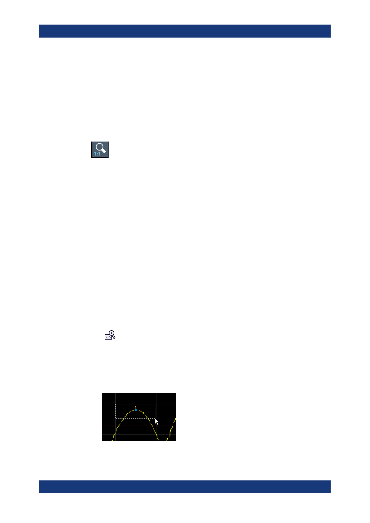
R&S®FSMR3-B60/B64
Y-Lock ← Measurement Zoom
If activated, the y-axis of the diagram is not changed during subsequent touch gestures.
Adapt Measurement to Zoom (selected diagram) ← Measurement Zoom
If you already performed a graphical zoom using the "Single Zoom" on page 60 or
"Multi-Zoom" on page 60 functions, this function automatically adapts the measure-
ment settings to maintain the currently zoomed display.
Restore Original Display
Restores the original display, that is, the originally calculated displays for the entire
capture buffer, and closes all zoom windows.
Note: This function only restores graphically zoomed displays. Measurement zooms,
for which measurement settings were adapted, are recalculated based on the adapted
measurement settings. In this case, the zoomed display is maintained.
Remote command:
DISPlay[:WINDow<n>][:SUBWindow<w>]:ZOOM[:STATe] on page 176
Common analysis and display functions
Zoomed displays
4.1.3 How to zoom into a diagram
The following tasks are described here:
●
"To zoom into the diagram at one position" on page 62
●
"To return to original display" on page 63
●
"To zoom into multiple positions in the diagram" on page 63
●
"To maintain a zoomed display permanently" on page 64
To zoom into the diagram at one position
1.
Click on the "Single Zoom" icon in the toolbar.
Zoom mode is activated.
2. Tap and drag your finger in the diagram to select the area to be enlarged. The
selected area is indicated by a dotted rectangle.
62User Manual 1179.0145.02 ─ 02
Page 63

R&S®FSMR3-B60/B64
3. Repeat these steps, if necessary, to enlarge the diagram further.
Scrolling in the zoomed display
You can scroll the diagram area to display the entire diagram using the scrollbars at the
right and at the bottom of the diagram.
To return to original display
Common analysis and display functions
Zoomed displays
When you leave the touchscreen, the diagram is replaced by the zoomed trace
area.
►
Click on the "Zoom Off" icon in the toolbar.
The original trace display is restored. Zoom mode remains active, however.
To zoom into multiple positions in the diagram
1.
Click on the "Multi-Zoom" icon in the toolbar.
Multiple zoom mode is activated.
2. Select the first area in the diagram to be enlarged as described in "To zoom into
the diagram at one position" on page 62. The selected area is indicated by a dotted
rectangle.
When you have completed your selection, the original trace is shown in an over-
view diagram with the selected area indicated by a dotted rectangle. The zoomed
trace area is displayed in a separate window (see Chapter 4.1.1, "Single zoom ver-
sus multiple zoom", on page 59.
3.
Click on the "Multi-Zoom" icon in the toolbar again.
4. In the overview diagram, select the next area to be enlarged.
The second zoom area is indicated in the overview diagram, and a second zoom
window is displayed.
63User Manual 1179.0145.02 ─ 02
Page 64

R&S®FSMR3-B60/B64
5. Repeat these steps, if necessary, to zoom into further trace areas (up to four).
To move or change zoom areas
In multiple zoom mode, you can change the size or position of the individual zoom
areas easily at any time.
► To resize a zoom area, tap directly on the corresponding frame in the overview
To maintain a zoomed display permanently
Graphical zooming only changes the resolution of the displayed trace points temporarily. In order to change the display permanently, you must change the corresponding
measurement settings.
(Note: Performing a measurement zoom automatically adapts the measurement settings to reflect a graphically zoomed display, see "To perform a measurement zoom"
on page 64).
Common analysis and display functions
Zoomed displays
window and drag the line to change the size of the frame.
To move a zoom area, tap inside the corresponding frame in the overview window
and drag the frame to the new position.
The contents of the zoom windows are adapted accordingly.
1. Perform a graphical zoom as described in the previous procedures.
2. Select the "Measurement Zoom" icon from the toolbar.
3. Select "Adapt Hardware to Zoom (selected diagram)".
The measurement settings are adapted as required to obtain the zoomed result
display.
To perform a measurement zoom
Performing a measurement zoom automatically adapts the measurement settings to
reflect a graphically zoomed display.
1. Select the "Measurement Zoom" icon from the toolbar.
2. Do one of the following to define the zoom area:
● Stretch two fingers in the diagram to enlarge the area between them.
● Tap and drag one finger in the diagram to select the area to be enlarged. The
selected area is indicated by a dotted rectangle.
The measurement settings are adapted as required to obtain the zoomed result
display.
64User Manual 1179.0145.02 ─ 02
Page 65

R&S®FSMR3-B60/B64
4.2 Trace configuration
● Basics on traces......................................................................................................65
● Trace configuration................................................................................................. 68
● Trace export and import..........................................................................................71
● Copying traces........................................................................................................ 76
● Trace math..............................................................................................................76
● Trace labels.............................................................................................................77
● How to configure traces.......................................................................................... 78
● References..............................................................................................................79
4.2.1 Basics on traces
● Analyzing several traces - trace mode....................................................................65
● Trace averaging...................................................................................................... 66
● Spurs and spur removal..........................................................................................67
Common analysis and display functions
Trace configuration
4.2.1.1 Analyzing several traces - trace mode
If several sweeps are performed one after the other, or continuous sweeps are performed, the trace mode determines how the data for subsequent traces is processed.
After each sweep, the trace mode determines whether:
●
The data is frozen ("View")
●
The data is hidden ("Blank")
●
The data is replaced by new values ("Clear Write")
●
The data is replaced selectively ("Max Hold", "Min Hold", "Average")
Each time you change the trace mode, the selected trace memory is cleared.
The R&S FSMR3 supports the following trace modes:
Table 4-1: Overview of available trace modes
Trace Mode Description
Blank Hides the selected trace.
Clear Write Overwrite mode: the trace is overwritten by each sweep. This is the default setting.
All available detectors can be selected.
Max Hold The maximum value is determined over several measurements and displayed. The
R&S FSMR3 saves the sweep result in the trace memory only if the new value is
greater than the previous one.
Min Hold The minimum value is determined from several measurements and displayed. The
R&S FSMR3 saves the sweep result in the trace memory only if the new value is
lower than the previous one.
65User Manual 1179.0145.02 ─ 02
Page 66

R&S®FSMR3-B60/B64
Trace Mode Description
Average The average is formed over several measurements and displayed.
View The current contents of the trace memory are frozen and displayed.
Write Hold The trace is overwritten when new data is available, but only after all cross-correlation
If a trace is frozen ("View" mode), you can change the measurement settings, apart
from scaling settings, without impact on the displayed trace. The fact that the displayed
trace no longer matches the current measurement settings is indicated by a yellow
asterisk
If you change any parameters that affect the scaling of the diagram axes, the
R&S FSMR3 automatically adapts the trace data to the changed display range. Thus,
you can zoom into the diagram after the measurement to show details of the trace.
Common analysis and display functions
Trace configuration
The Sweep/Average Count determines the number of averaging procedures.
operations defined for a half decade are done.
on the tab label.
4.2.1.2 Trace averaging
The application provides several methods of trace averaging that you can use separately or in any combination.
The order in which averaging is performed is as follows.
1. Cross-correlation
The application performs a certain number of cross-correlation operations in each
half decade.
2. Sweep count.
The application measures the complete measurement range a particular number of
times.
It again includes the cross-correlation operations as defined.
After the measurement over the sweep count is finished, the application displays
the averaged results.
3. Trace smoothing.
Calculates the moving average for the current trace.
Sweep count
The sweep count defines the number of sweeps that the application performs during a
complete measurements.
A sweep in this context is the measurement over the complete measurement range
once. A complete measurement, however, can consist of more than one sweep. In that
case, the application measures until the number of sweeps that have been defined are
done. The measurement configuration stays the same all the time.
66User Manual 1179.0145.02 ─ 02
Page 67

R&S®FSMR3-B60/B64
In combination with the average trace mode and cross-correlation operations, the
sweep count averages the trace even more.
Trace smoothing
(Software-based) smoothing is a way to remove anomalies visually in the trace that
can distort the results. The smoothing process is based on a moving average over the
complete measurement range. The number of samples included in the averaging process (the aperture size) is variable and is a percentage of all samples that the trace consists of.
Figure 4-3: Sample size included in trace smoothing
Common analysis and display functions
Trace configuration
The application smoothes the trace continuously. Smoothing is just an enhancement of
the trace display, not of the data itself. It is always applied before trace averaging, max
hold, min hold or write hold. For the smoothing process, a median filter is applied on
the logarithmic data.
You can turn trace smoothing on and off for all traces individually and compare, for
example, the raw and the smooth trace.
The median trace smoothing uses a median filter which takes the median value over a
sliding window. The window size can be set in the trace menu in percent of the total
evaluation range. A median filter suppresses outliers while smoothing the underlying
noise curve.
4.2.1.3 Spurs and spur removal
Most phase noise results contain unwanted spurs. Spurs are peak levels at one or
more offset frequencies and are caused mostly by interfering signals. For some applications, you might want to identify the location of spurs. For other applications, spurs
do not matter in evaluating the results and you might want to remove them from the
trace to get a "smooth" phase noise trace.
Spur display
Usually, spurs are visible on the trace as a peak. In addition, the R&S FSMR3 draws a
straight, vertical line to represent the position of a spur visually. The length of these
lines indicates the level of the spur in dBc and refers to the scale on the right side of
the phase noise diagram.
The lines indicating a spur are not part of the trace data. When you export the trace, for
example, the spur data is not exported.
67User Manual 1179.0145.02 ─ 02
Page 68

R&S®FSMR3-B60/B64
Spur suppression
The application allows you to (visually) remove spurs from the trace. Spur removal is
based on an algorithm that detects and completely removes the spurs from the trace
and fills the gaps with data that has been determined mathematically.
The spur removal functionality separates the actual spur power from the underlying
phase noise and displays the latter in a two-stage process. The first stage of spur
detection is based on an eigenvalue decomposition during the signal processing.
Spur threshold
During the second stage, the application uses statistical methods to remove a spur. A
spur is detected, if the level of the signal is above a certain threshold. The spur threshold is relative to an imaginary median trace that the application calculates.
If parts of the signal are identified as spurs, the application removes all signal parts
above that level and substitutes them with the median trace.
Common analysis and display functions
Trace configuration
Figure 4-4: Spur detection and removal principle
4.2.2 Trace configuration
Access: "Overview" > "Analysis" > "Traces" > "Traces"
Traces are the graphical representation of the measurement results. Depending on the
trace configuration, they carry different information or evaluate the results differently.
68User Manual 1179.0145.02 ─ 02
Page 69

R&S®FSMR3-B60/B64
Restoring default traces
The application allows you to easily restore the default trace configuration (Trace 1 and
2 with their respective default characteristics) with the "Preset all Traces" button.
Common analysis and display functions
Trace configuration
Displaying all result types
Similarly, you can easily display all available result type (PM, AM and overall noise)
with the "Set Result Type" button. When you do so, the application displays three
traces in the diagram: One for the phase noise, one for the AM noise and the third
showing the sum of the phase noise and AM noise (PN + AM).
Functions in the "Traces" dialog box described elsewhere:
●
Chapter 4.2.1.3, "Spurs and spur removal", on page 67
Trace 1/Trace 2/Trace 3/Trace 4/Trace 5/Trace 6
Selects the corresponding trace for configuration. The currently selected trace is highlighted.
Remote command:
Selected via numeric suffix of:TRACe<1...6> commands
DISPlay[:WINDow<n>][:SUBWindow<w>]:TRACe<t>[:STATe] on page 180
Trace Mode
Defines the update mode for subsequent traces.
For details, see Chapter 4.2.1.1, "Analyzing several traces - trace mode", on page 65.
"Clear/ Write"
"Max Hold"
"Min Hold"
Overwrite mode (default): the trace is overwritten by each sweep.
The maximum value is determined over several sweeps and dis-
played. The R&S FSMR3 saves each trace point in the trace memory
only if the new value is greater than the previous one.
The minimum value is determined from several measurements and
displayed. The R&S FSMR3 saves each trace point in the trace memory only if the new value is lower than the previous one.
69User Manual 1179.0145.02 ─ 02
Page 70

R&S®FSMR3-B60/B64
Common analysis and display functions
Trace configuration
"Average"
"View"
"Blank"
"Write Hold"
Remote command:
DISPlay[:WINDow<n>][:SUBWindow<w>]:TRACe<t>:MODE on page 177
Selecting the displayed result
The R&S FSMR3 supports several noise characteristics that you can assign to a trace
and thus display in the diagram.
●
"Phase Noise"
Shows the measured phase noise characteristics.
●
"AM Noise"
Shows the measured amplitude noise characteristics.
●
"Phase + AM Noise"
Shows the sum of the phase noise and AM noise characteristics.
The "AM Noise" and "Phase + AM Noise" traces are only available for the "Noise Spectrum" diagram, and not in its variations ("Noise Spectrum L(f)", "Noise Spectrum
SΦ(f)", "Noise Spectrum Sv(f)", "Noise Spectrum Sy(f)").
The average is formed over several sweeps.
The current contents of the trace memory are frozen and displayed.
Removes the selected trace from the display.
The trace is overwritten when new data is available, but only after all
cross-correlation operations defined for a half decade are done. (Or
when the trace cannot be improved further when "XCORR Optimization" is on).
Example: 100 cross-correlation operations are defined for a half decade. The trace is updated when all 100 cross-correlations are done,
not after each individual cross-correlation operation.
Remote command:
DISPlay[:WINDow<n>]:TRACe<t>:RESult[:TYPE] on page 180
Smoothing traces
The R&S FSMR3 allows you to smooth traces and thus remove unwanted anomalies.
You can apply smoothing to all active traces individually (Smoothing "State"), and
define the magnitude of trace smoothing in percent (Smoothing "Value").
The range is from 1% to 20%.
Remote command:
State: DISPlay[:WINDow<n>]:TRACe<t>:SMOothing[:STATe] on page 182
Value: DISPlay[:WINDow<n>]:TRACe<t>:SMOothing:APERture on page 182
Removing spurs
Spur removal is a method to remove displayed peak levels visually.
You can apply spur removal to all active traces individually (spurious removal "State"),
and define a threshold (in dB) that defines when a peak level is recognized as a spur
(spurious removal "Value").
More information
70User Manual 1179.0145.02 ─ 02
Page 71

R&S®FSMR3-B60/B64
Remote command:
State: DISPlay[:WINDow<n>]:TRACe<t>:SPURs:SUPPress on page 161
Value: DISPlay[:WINDow<n>]:TRACe<t>:SPURs:THReshold on page 162
Shifting the trace
Shifting the trace can be useful to subtract external noise sources from the results. The
trace offset is a visual device that shifts the trace by certain level.
You can apply an offset to all active traces individually (Offset "State"), and define an
offset in dB by which the trace should be shifted.
Remote command:
State: DISPlay[:WINDow<n>]:TRACe<t>:Y[:SCALe]:RLEVel:OFFSet:STATe
on page 181
Offset: DISPlay[:WINDow<n>]:TRACe<t>:Y[:SCALe]:RLEVel:OFFSet
on page 181
Displaying persistence
The term persistence has its origins in cathode ray tube devices (CRTs). It describes
the time period one point on the display stays illuminated after it has been lit by the
cathode ray. The higher the persistence, the longer you could observe the illuminated
point on the display.
In the phase noise application, the persistence defines for how long a trace remains
visible before it fades away. An event that has occurred a single time is visible for up to
8 seconds. As the statistical frequency of an event gets smaller at coordinates with signal parts that are not constantly there, the trace fades away.
A signal with constant frequency or phase characteristics does not show the effects of
persistence on the trace. When the frequency or phase of a signal change slightly,
however, the effect of persistence becomes visible through color changes or changes
in the shape of the trace.
You can turn on persistence for all traces in the display ("State"). The "Decay" property
defines the time that shadows of past traces remain visible in the display before fading
away. With a decay of 0 s, all past traces remain visible.
Common analysis and display functions
Trace configuration
When you change a measurement setting, the R&S FSMR3 resets the persistence
effect.
Persistence is supported by phase noise measurements.
Remote command:
DISPlay[:WINDow<n>]:TRACe<t>:PERSistence[:STATe] on page 180
DISPlay[:WINDow<n>]:TRACe<t>:PERSistence:DECay on page 179
4.2.3 Trace export and import
Access: "Overview" > "Analysis" > "Traces" > "Trace / Data Export"
The R&S FSMR3 provides various evaluation methods for the results of a measurement. However, if you want to evaluate the data with external applications, you can
export the measurement data to a standard format file (ASCII or XML).
71User Manual 1179.0145.02 ─ 02
Page 72

R&S®FSMR3-B60/B64
The following data types can be exported (depending on the application):
●
●
You can also import existing trace data from a file, for example to compare your latest
measurement results with results that you have saved some time ago.
I/Q data can only be imported and exported in applications that process I/Q data, such
as the I/Q analyzer or optional applications.
See the corresponding user manuals for those applications for details.
The standard data management functions (e.g. saving or loading instrument settings)
that are available for all R&S FSMR3 applications are not described here.
See the R&S FSMR3 user manual for a description of the standard functions.
Common analysis and display functions
Trace configuration
Trace data
Table results, for example result summaries, marker peak lists.
Export all Traces and all Table Results......................................................................... 72
Include Instrument & Measurement Settings................................................................ 73
Trace to Export..............................................................................................................73
Export Trace to ASCII File.............................................................................................73
└ File Type......................................................................................................... 74
└ Decimal Separator.......................................................................................... 74
└ Column Separator...........................................................................................74
└ File Explorer....................................................................................................75
Select ASCII File...........................................................................................................75
Source Window / Source Trace.....................................................................................75
Destination Trace..........................................................................................................75
Import............................................................................................................................76
Export all Traces and all Table Results
Selects all displayed traces and result tables (e.g. "Result Summary", marker table
etc.) in the current application for export to an ASCII file.
Alternatively, you can select one specific trace only for export (see Trace to Export).
The results are output in the same order as they are displayed on the screen: window
by window, trace by trace, and table row by table row.
72User Manual 1179.0145.02 ─ 02
Page 73

R&S®FSMR3-B60/B64
Remote command:
FORMat:DEXPort:TRACes on page 186
Include Instrument & Measurement Settings
Includes additional instrument and measurement settings in the header of the export
file for result data.
Remote command:
FORMat:DEXPort:HEADer on page 185
Trace to Export
Defines an individual trace to be exported to a file.
This setting is not available if Export all Traces and all Table Results is selected.
Export Trace to ASCII File
Saves the selected trace or all traces in the currently active result display to the specified file and directory in the selected ASCII format.
"File Explorer": Instead of using the file manager of the R&S FSMR3 firmware, you can
also use the Microsoft Windows File Explorer to manage files.
Common analysis and display functions
Trace configuration
73User Manual 1179.0145.02 ─ 02
Page 74

R&S®FSMR3-B60/B64
For details on the file format, see Chapter 4.2.8.1, "Reference: ASCII file export for-
mat", on page 79.
Note: Secure user mode.
In secure user mode, settings that are stored on the instrument are stored to volatile
memory, which is restricted to 256 MB. Thus, a "memory limit reached" error can occur
although the hard disk indicates that storage space is still available.
To store data permanently, select an external storage location such as a USB memory
device.
For details, see "Protecting Data Using the Secure User Mode" in the "Data Management" section of the R&S FSMR3 User Manual.
Remote command:
MMEMory:STORe<n>:TRACe on page 187
File Type ← Export Trace to ASCII File
Determines the format of the ASCII file to be imported or exported.
Depending on the external program in which the data file was created or is evaluated,
a comma-separated list (CSV) or a plain data format (DAT) file is required.
Common analysis and display functions
Trace configuration
Remote command:
FORMat:DEXPort:FORMat on page 185
Decimal Separator ← Export Trace to ASCII File
Defines the decimal separator for floating-point numerals for the data export/import
files. Evaluation programs require different separators in different languages.
Remote command:
FORMat:DEXPort:DSEParator on page 185
Column Separator ← Export Trace to ASCII File
Selects the character that separates columns in the exported ASCII file. The character
can be either a semicolon, a comma or a tabulator (tab).
Example for semicolon:
Type;FSMR3026;Version;1.80;Date;01.Jan 3000;
Example for comma:
Type,FSMR3026,
Version,1.80,
Date,01.Jan 3000,
Example for tabulator (tab after the last column is not visible):
Type FSMR3026
Version 1.80
Date 01.Jan 3000
The selected column separator setting remains the same, even after a preset.
Remote command:
FORMat:DEXPort:CSEParator on page 184
74User Manual 1179.0145.02 ─ 02
Page 75

R&S®FSMR3-B60/B64
File Explorer ← Export Trace to ASCII File
Opens the Microsoft Windows File Explorer.
Remote command:
not supported
Select ASCII File
The "Select ASCII File" button opens a dialog box to select results that you want to
import.
You can select files with the extensions .csv or .dat.
Remote command:
MMEMory:LOAD<n>:TRACe on page 186
Source Window / Source Trace
Files that contain result data can contain the results of several measurements and
result displays. The "Source Window" and "Source Trace" dropdown menus select the
data that you would like to import.
The source data must be compatible to a currently active window.
Common analysis and display functions
Trace configuration
Example:
If you want to import trace 1 of a previously exported noise diagram:
●
Select the phase noise measurement and open a noise diagram from the SmartGrid.
●
Select "Noise Diagram" from the "Source Window" dropdown menu.
●
Select "1" from the "Source Trace" dropdown menu.
If you select "All Traces", the R&S FSMR3 imports all traces of the selected result
type.
Remote command:
MMEMory:LOAD<n>:TRACe on page 186
Destination Trace
The "Destination Trace" dropdown menu becomes available when you select to import
a single trace only.
In that case, you can select the trace number you want to write the trace data to.
If you select a trace that already exists, the trace import overwrites the currently dis-
played trace. Imported traces always get the trace mode "View".
Example:
You have selected trace "1" as the trace you want to import from the "Source Trace"
dropdown menu.
If you select "1: Clear Write" ("Clear Write" indicates the trace is currently displayed)
from the "Destination Trace" dropdown menu, the import overwrites the trace. The
trace mode for trace 1 is replaced by trace mode "View".
If you select "5: Blank" ("Blank" indicates that the trace is currently not displayed) from
the "Destination Trace" dropdown menu, the imports adds a new trace to the diagram
(with trace mode "View". All other traces remain in the diagram.
75User Manual 1179.0145.02 ─ 02
Page 76

R&S®FSMR3-B60/B64
Remote command:
MMEMory:LOAD<n>:TRACe on page 186
Import
The "Import" button imports the selected trace(s).
THe R&S FSMR3 does not import numeric results associated with the imported trace
(spot noise, values from the spurious list etc.)
Remote command:
MMEMory:LOAD<n>:TRACe on page 186
4.2.4 Copying traces
Access: "Overview" > "Analysis" > "Traces" > "Copy Trace"
Common analysis and display functions
Trace configuration
Copy Trace....................................................................................................................76
Copy Trace
Access: "Overview" > "Analysis" > "Traces" > "Copy Trace"
Or: [TRACE] > "Copy Trace"
Copies trace data to another trace.
Remote command:
TRACe<n>:COPY on page 183
4.2.5 Trace math
Access: "Overview" > "Analysis" > "Traces" > "Trace Math"
76User Manual 1179.0145.02 ─ 02
Page 77

R&S®FSMR3-B60/B64
Selecting the math operation........................................................................................ 77
Selecting the math operation
You can select one of several different math operations.
Each operation subtracts one trace from another as indicated on the corresponding
button and writes the result to one of the traces. "T1 - T3 > T1", for example, subtracts
trace 3 from trace 1 and writes the result to trace 1. You can apply one operation at a
time.
To turn off trace mathematics, use the "Trace Math Off" feature.
Remote command:
Operation: CALCulate<n>:MATH[:EXPRession][:DEFine] on page 188
State: CALCulate<n>:MATH:STATe on page 188
Common analysis and display functions
Trace configuration
4.2.6 Trace labels
Access: "Overview" > "Analysis" > "Traces" > "Trace Label"
Trace labels are a way to assign a descriptive label to traces instead of the general
"Trace <x>" label (default). The labels you use are arbitrary and are displayed in the
diagram area. The font color corresponds to the color of the respective trace (for example yellow trace: yellow font).
Figure 4-5: Example: the yellow and blue traces have a label.
You can define trace labels in the "Trace Label" tab of the "Trace" dialog box.
77User Manual 1179.0145.02 ─ 02
Page 78

R&S®FSMR3-B60/B64
How to assign trace labels
Common analysis and display functions
Trace configuration
Trace labels can be configured via the "Trace Labels" dialog box.
1. Turn on the trace label for a specific trace and assign a label in the corresponding
input field.
Note that a trace must be active. Otherwise assigning a label is not possible.
2. Move the trace label to any position on the display by dragging it to the new posi-
tion.
Remote command:
State: DISPlay[:WINDow<n>]:TRACe<t>:LABel[:STATe] on page 178
Label: DISPlay[:WINDow<n>]:TRACe<t>:LABel:TEXT on page 179
4.2.7 How to configure traces
● How to export trace data and numerical results......................................................78
4.2.7.1 How to export trace data and numerical results
The measured trace data and numerical measurement results in tables can be exported to an ASCII file. For each sweep point, the measured trace position and value are
output. The file is stored with a .DAT extension. For details on the storage format, see
Chapter 4.2.8.1, "Reference: ASCII file export format", on page 79.
To export trace data and table results
Trace data can be exported from the "Trace" menu.
1. Press the [Trace] key, then select the "Trace Config" softkey and switch to the
"Trace / Data Export" tab.
78User Manual 1179.0145.02 ─ 02
Page 79

R&S®FSMR3-B60/B64
2. Select "Export all Traces and all Table Results" to export all available measurement
3. Optionally, select the "Include Instrument & Measurement Settings" option to insert
4. If necessary, change the decimal separator used in the ASCII export file.
5. Select the "Export Trace to ASCII File" button.
6. In the file selection dialog box, select the storage location and file name for the
7. Select "Save" to close the dialog box.
8. Export the data to the file.
4.2.8 References
Common analysis and display functions
Markers
result data for the current application. Alternatively, select a specific "Trace to
Export".
additional information in the export file header.
export file.
● Reference: ASCII file export format........................................................................ 79
4.2.8.1 Reference: ASCII file export format
Trace data can be exported to a file in ASCII format for further evaluation in other applications. This reference describes in detail the format of the export files for result data.
(For details see Chapter 4.2.7.1, "How to export trace data and numerical results",
on page 78).
The file consists of the header information (general configuration of the measurement)
and the measurement results. Optionally, the header can be excluded from the file.
The data of the file header consist of three columns, each separated by a semicolon:
parameter name; numeric value; basic unit. The data section starts with the keyword
"Trace <n>" (<n> = number of stored trace). The measured data follows in one or several columns (depending on the measurement), which are also separated by a semicolon.
The results are output in the same order as they are displayed on the screen: window
by window, trace by trace, and table row by table row.
Generally, the format of this ASCII file can be processed by spreadsheet calculation
programs, e.g. MS Excel. Different language versions of evaluation programs can
require a different handling of the decimal point. Thus, you can define the decimal separator to use (decimal point or comma).
4.3 Markers
Markers help you analyze your measurement results by determining particular values
in the diagram. Thus you can extract numeric values from a graphical display.
79User Manual 1179.0145.02 ─ 02
Page 80

R&S®FSMR3-B60/B64
● Basics on markers and marker functions................................................................80
● Marker settings........................................................................................................82
● Marker search settings and positioning functions................................................... 86
4.3.1 Basics on markers and marker functions
Some background knowledge on marker settings and functions is provided here for a
better understanding of the required configuration settings.
Markers are used to mark points on traces, to read out measurement results and to
select a display section quickly. R&S FSMR3 provides 16 markers per display window.
In the Phase Noise application, markers across measurement windows are independent from each other - thus you can move a marker in one window without moving it in
another window.
●
Common analysis and display functions
Markers
The easiest way to work with markers is using the touchscreen. Simply drag the
marker and drop it at the required position. When a marker label is selected, a vertical line is displayed which indicates the marker's current x-value.
●
Alternatively, change the position of the selected marker using the rotary knob. By
default, the marker is moved from one pixel to the next.
●
You can also set an active marker to a new position by defining its position on the
x-axis numerically. When you select the softkey for a marker, an edit dialog box is
displayed.
●
The most commonly required marker settings and functions are also available as
softkeys or via the context menu. Tap the marker on the touchscreen and hold your
finger for about 2 seconds until the context menu is opened, then select the
required entry.
●
Softkeys for active markers (displayed on the screen) are highlighted blue. The
softkey for the currently selected marker (for which functions are performed) is
highlighted orange.
●
To set individual markers quickly, use the softkeys in the "Marker" menu.
●
To set up several markers at once, use the "Marker" dialog box.
●
To position the selected marker to a special value, use the softkeys in the "Marker
To" menu.
Marker types
All markers can be used either as normal markers or delta markers. A normal marker
indicates the absolute signal value at the defined position in the diagram. A delta
80User Manual 1179.0145.02 ─ 02
Page 81

R&S®FSMR3-B60/B64
marker indicates the value of the marker relative to the specified reference marker (by
default marker 1).
● Activating markers...................................................................................................81
● Marker results......................................................................................................... 81
4.3.1.1 Activating markers
Only active markers are displayed in the diagram and in the marker table.
Active markers are indicated by a highlighted softkey.
By default, marker 1 is active and positioned on the maximum value (peak) of trace 1
as a normal marker. If several traces are displayed, the marker is set to the maximum
value of the trace which has the lowest number and is not frozen (View mode). The
next marker to be activated is set to the frequency of the next lower level (next peak)
as a delta marker; its value is indicated as an offset to marker 1.
A marker can only be activated when at least one trace in the corresponding window is
visible. If a trace is switched off, the corresponding markers and marker functions are
also deactivated. If the trace is switched on again, the markers along with coupled
functions are restored to their original positions, provided the markers have not been
used on another trace.
Common analysis and display functions
Markers
4.3.1.2 Marker results
Normal markers point to a trace point on the x-axis and display the associated numeric
value for that trace point. Delta markers indicate an offset between the level at the
delta marker position and the level at the position of the assigned reference marker, in
dB.
The results can be displayed directly within the diagram area or in a separate table. By
default, the first two active markers are displayed in the diagram area. If more markers
are activated, the results are displayed in a marker table.
Marker information in diagram area
By default, the results of the last two markers or delta markers that were activated are
displayed in the diagram area.
The following information is displayed there:
●
The marker type (M for normal, D for delta, or special function name)
●
The marker number (1 to 16)
●
The assigned trace number in square brackets [ ]
●
The marker value on the y-axis, or the result of the marker function
●
The marker position on the x-axis
81User Manual 1179.0145.02 ─ 02
Page 82

R&S®FSMR3-B60/B64
Marker information in marker table
In addition to the marker information displayed within the diagram area, a separate
marker table may be displayed beneath the diagram. This table provides the following
information for all active markers:
Table 4-2: Contents of the marker table in the Phase Noise application
Window Window the marker is in (only if you have opened more than one Phase Noise dia-
Type Marker type: N (normal), D (delta), T (temporary, internal) and number
Ref Reference marker for delta markers
Trc Trace to which the marker is assigned
X-value X-value of the marker
Y-value Y-value of the marker
4.3.2 Marker settings
Common analysis and display functions
Markers
gram)
For more information about marker search, see Chapter 4.3.3, "Marker search settings
and positioning functions", on page 86
● Individual marker setup...........................................................................................82
● General marker settings..........................................................................................85
4.3.2.1 Individual marker setup
Access: "Overview" > "Analysis" > "Markers" > "Markers"
Up to 17 markers or delta markers can be activated for each window simultaneously.
Initial marker setup is performed using the "Marker" dialog box.
The markers are distributed among 3 tabs for a better overview. By default, the first
marker is defined as a normal marker, whereas all others are defined as delta markers
with reference to the first marker. All markers are assigned to trace 1, but only the first
marker is active.
82User Manual 1179.0145.02 ─ 02
Page 83

R&S®FSMR3-B60/B64
Common analysis and display functions
Markers
Selected Marker............................................................................................................83
Marker State..................................................................................................................83
Marker Position X-value................................................................................................83
Marker Type..................................................................................................................84
Reference Marker......................................................................................................... 84
Linking to Another Marker.............................................................................................84
Assigning the Marker to a Trace................................................................................... 84
Select Marker................................................................................................................85
All Markers Off...............................................................................................................85
Selected Marker
Marker name. The marker which is currently selected for editing is highlighted orange.
Remote command:
Marker selected via suffix <m> in remote commands.
Marker State
Activates or deactivates the marker in the diagram.
Remote command:
CALCulate<n>:MARKer<m>[:STATe] on page 194
CALCulate<n>:DELTamarker<m>[:STATe] on page 192
Marker Position X-value
Defines the position (x-value) of the marker in the diagram. For normal markers, the
absolute position is indicated. For delta markers, the position relative to the reference
marker is provided.
Remote command:
CALCulate<n>:MARKer<m>:X on page 195
CALCulate<n>:DELTamarker<m>:X on page 193
83User Manual 1179.0145.02 ─ 02
Page 84

R&S®FSMR3-B60/B64
Marker Type
Toggles the marker type.
The type for marker 1 is always "Normal", the type for delta marker 1 is always "Delta".
These types cannot be changed.
Note: If normal marker 1 is the active marker, switching the "Mkr Type" activates an
additional delta marker 1. For any other marker, switching the marker type does not
activate an additional marker, it only switches the type of the selected marker.
"Normal"
"Delta"
Remote command:
CALCulate<n>:MARKer<m>[:STATe] on page 194
CALCulate<n>:DELTamarker<m>[:STATe] on page 192
Reference Marker
Defines a marker as the reference marker which is used to determine relative analysis
results (delta marker values).
If the reference marker is deactivated, the delta marker referring to it is also deactivated.
Remote command:
CALCulate<n>:DELTamarker<m>:MREFerence on page 192
Common analysis and display functions
Markers
A normal marker indicates the absolute value at the defined position
in the diagram.
A delta marker defines the value of the marker relative to the specified reference marker (marker 1 by default).
Linking to Another Marker
Links the current marker to the marker selected from the list of active markers. If the xaxis value of the initial marker is changed, the linked marker follows to the same position on the x-axis. Linking is off by default.
Using this function you can set two markers on different traces to measure the difference (e.g. between a max hold trace and a min hold trace or between a measurement
and a reference trace).
Remote command:
CALCulate<n>:MARKer<ms>:LINK:TO:MARKer<md> on page 193
CALCulate<n>:DELTamarker<ms>:LINK:TO:MARKer<md> on page 191
CALCulate<n>:DELTamarker<m>:LINK on page 190
Assigning the Marker to a Trace
The "Trace" setting assigns the selected marker to an active trace. The trace determines which value the marker shows at the marker position. If the marker was previously assigned to a different trace, the marker remains on the previous frequency or
time, but indicates the value of the new trace.
If a trace is turned off, the assigned markers and marker functions are also deactivated.
Remote command:
CALCulate<n>:MARKer<m>:TRACe on page 194
84User Manual 1179.0145.02 ─ 02
Page 85

R&S®FSMR3-B60/B64
Select Marker
The "Select Marker" function opens a dialog box to select and activate or deactivate
one or more markers quickly.
Common analysis and display functions
Markers
Remote command:
CALCulate<n>:MARKer<m>[:STATe] on page 194
CALCulate<n>:DELTamarker<m>[:STATe] on page 192
All Markers Off
Deactivates all markers in one step.
Remote command:
CALCulate<n>:MARKer<m>:AOFF on page 193
4.3.2.2 General marker settings
Access: "Overview" > "Analysis" > "Markers" > "Settings"
Some general marker settings allow you to influence the marker behavior for all markers.
85User Manual 1179.0145.02 ─ 02
Page 86

R&S®FSMR3-B60/B64
Marker Table Display.....................................................................................................86
Linked Markers..............................................................................................................86
Marker Table Display
Defines how the marker information is displayed.
"On"
"Off"
Remote command:
DISPlay[:WINDow<n>]:MTABle on page 195
Common analysis and display functions
Markers
Displays the marker information in a table in a separate area beneath
the diagram.
No separate marker table is displayed.
Linked Markers
If enabled, the markers in all diagrams with the same x-axis are linked, i.e. when you
move a marker in one window, the markers in all other windows are moved to the
same x-value.
Remote command:
CALCulate<n>:MARKer<m>:LINK on page 196
4.3.3 Marker search settings and positioning functions
Several functions are available to set the marker to a specific position quickly and
easily, or to use the current marker position to define another characteristic value. In
order to determine the required marker position, searches can be performed. The
search results can be influenced by special settings.
Most marker positioning functions and the search settings are available in the [MKR ➙]
menu.
Search settings are also available via the [Marker] key or in the vertical "Marker Config" tab of the "Analysis" dialog box (horizontal "Search Settings" tab).
● Marker search settings............................................................................................87
● Positioning functions............................................................................................... 88
86User Manual 1179.0145.02 ─ 02
Page 87

R&S®FSMR3-B60/B64
4.3.3.1 Marker search settings
Access: "Overview" > "Analysis" > "Markers" > "Search"
Markers are commonly used to determine peak values, i.e. maximum or minimum values, in the measured signal. Configuration settings allow you to influence the peak
search results.
Common analysis and display functions
Markers
Search Mode for Next Peak..........................................................................................87
Peak Excursion............................................................................................................. 87
Spurious Tracking......................................................................................................... 88
Search Mode for Next Peak
Selects the search mode for the next peak search.
"Left"
"Absolute"
"Right"
Remote command:
Find a list of remote commands in Chapter 6.6.4.4, "Positioning markers",
on page 197.
Peak Excursion
Defines the minimum level value by which a signal must rise or fall so that it is identified as a maximum or a minimum by the search functions.
Entries from 0 dB to 60 dB are allowed; the resolution is 0.1 dB. The default setting for
the peak excursion is 1 dB.
Determines the next maximum/minimum to the left of the current
peak.
Determines the next maximum/minimum to either side of the current
peak.
Determines the next maximum/minimum to the right of the current
peak.
Remote command:
CALCulate<n>:MARKer<m>:PEXCursion on page 196
87User Manual 1179.0145.02 ─ 02
Page 88

R&S®FSMR3-B60/B64
Spurious Tracking
Spurs can be unstable regarding their frequency characteristics. In such cases, markers would not remain on the spur, but on the frequency you have set them on initially.
You can avoid this situation using spurious tracking. Spur tracking makes sure that the
marker remains on the spur, even if the spur changes its frequency. When you turn on
spur tracking, you can define a frequency range within which the R&S FSMR3 tracks
the spur and adjusts the marker position automatically.
The tracking "Range" defines an area around the marker position and is a function of
the resolution bandwidth (RBW) used in the half decade the marker is in. Note that the
tracking range is dynamic and always relative to the latest marker position, not the initial marker position.
Example:
You are measuring with an RBW of 10 kHz and place the marker on a spur.
The tracking range is defined as 1 * RBW = 10 kHz.
If the spur changes its position by up to ±10 kHz, the R&S FSMR3 changes the marker
position along with the spur.
Common analysis and display functions
Markers
Note that the spurious list contains the tracked spurs and always shows the latest position of the spur.
Remote command:
State: CALCulate<n>:MARKer<m>:FUNCtion:SPTRacking[:STATe]
on page 197
Range: CALCulate<n>:MARKer<m>:FUNCtion:SPTRacking:RANGe on page 196
4.3.3.2 Positioning functions
Access: [MKR ➙]
The following functions set the currently selected marker to the result of a peak search
or set other characteristic values to the current marker value.
Peak Search..................................................................................................................88
Search Next Peak......................................................................................................... 88
Search Minimum........................................................................................................... 89
Search Next Minimum...................................................................................................89
Peak Search
Sets the selected marker/delta marker to the maximum of the trace. If no marker is
active, marker 1 is activated.
Remote command:
CALCulate<n>:MARKer<m>:MAXimum[:PEAK] on page 200
CALCulate<n>:DELTamarker<m>:MAXimum[:PEAK] on page 198
Search Next Peak
Sets the selected marker/delta marker to the next (lower) maximum of the assigned
trace. If no marker is active, marker 1 is activated.
88User Manual 1179.0145.02 ─ 02
Page 89

R&S®FSMR3-B60/B64
Remote command:
CALCulate<n>:MARKer<m>:MAXimum:NEXT on page 200
CALCulate<n>:MARKer<m>:MAXimum:RIGHt on page 200
CALCulate<n>:MARKer<m>:MAXimum:LEFT on page 200
CALCulate<n>:DELTamarker<m>:MAXimum:NEXT on page 198
CALCulate<n>:DELTamarker<m>:MAXimum:RIGHt on page 198
CALCulate<n>:DELTamarker<m>:MAXimum:LEFT on page 198
Search Minimum
Sets the selected marker/delta marker to the minimum of the trace. If no marker is
active, marker 1 is activated.
Remote command:
CALCulate<n>:MARKer<m>:MINimum[:PEAK] on page 201
CALCulate<n>:DELTamarker<m>:MINimum[:PEAK] on page 199
Search Next Minimum
Sets the selected marker/delta marker to the next (higher) minimum of the selected
trace. If no marker is active, marker 1 is activated.
Remote command:
CALCulate<n>:MARKer<m>:MINimum:NEXT on page 201
CALCulate<n>:MARKer<m>:MINimum:LEFT on page 200
CALCulate<n>:MARKer<m>:MINimum:RIGHt on page 201
CALCulate<n>:DELTamarker<m>:MINimum:NEXT on page 199
CALCulate<n>:DELTamarker<m>:MINimum:LEFT on page 199
CALCulate<n>:DELTamarker<m>:MINimum:RIGHt on page 199
Common analysis and display functions
Limit lines
4.4 Limit lines
Limit lines help you analyze a measurement trace.
● Basics on limit lines.................................................................................................89
● Limit line settings and functions.............................................................................. 93
● How to define limit lines.......................................................................................... 98
4.4.1 Basics on limit lines
Limit lines are used to define amplitude curves or spectral distribution boundaries in
the result diagram which are not to be exceeded. They indicate, for example, the upper
limits for interference radiation or spurious waves which are allowed from a device
under test (DUT). When transmitting information in TDMA systems (e.g. GSM), the
amplitude of the bursts in a time slot must adhere to a curve that falls within a specified
tolerance band. The lower and upper limits may each be specified by a limit line. Then,
the amplitude curve can be controlled either visually or automatically for any violations
of the upper or lower limits (GO/NOGO test).
89User Manual 1179.0145.02 ─ 02
Page 90

R&S®FSMR3-B60/B64
The R&S FSMR3 supports limit lines with a maximum of 200 data points. Eight of the
limit lines stored in the instrument can be activated simultaneously. The number of limit
lines stored in the instrument is only limited by the capacity of the storage device used.
Limit line data can also be exported to a file in ASCII (CSV) format for further evaluation in other applications. Limit lines stored in the specified ASCII (CSV) format can
also be imported to the R&S FSMR3 for other measurements.
Compatibility
Limit lines are compatible with the current measurement settings, if the following
applies:
●
●
Validity
Only limit lines that fulfill the following conditions can be activated:
●
●
●
●
Common analysis and display functions
Limit lines
The x unit of the limit line has to be identical to the current setting.
The y unit of the limit line has to be identical to the current setting.
Each limit line must consist of a minimum of 2 and a maximum of 200 data points.
The frequencies/times for each data point must be defined in ascending order;
however, for any single frequency or time, two data points may be entered (to
define a vertical segment of a limit line).
Gaps in frequency or time are not allowed. If gaps are desired, two separate limit
lines must be defined and then both enabled.
The entered frequencies or times need not necessarily be selectable in
R&S FSMR3. A limit line may also exceed the specified frequency or time range.
The minimum frequency for a data point is -200 GHz, the maximum frequency is
200 GHz. For the time range representation, negative times may also be entered.
The allowed range is -1000 s to +1000 s.
90User Manual 1179.0145.02 ─ 02
Page 91

R&S®FSMR3-B60/B64
Common analysis and display functions
Limit lines
Figure 4-6: Example for an upper limit line
Thresholds
If the y-axis for the limit line data points uses relative scaling, an additional absolute
threshold can be defined for the limit check. In this case, both the threshold value and
the relative limit line must be exceeded before a violation occurs.
Offsets and Shifting
A configured limit line can easily be moved vertically or horizontally. Two different
methods to do so are available:
●
An offset moves the entire line in the diagram without editing the configured values
or positions of the individual data points. This option is only available if relative
scaling is used.
Thus, a new limit line can be easily generated based upon an existing limit line
which has been shifted horizontally or vertically.
91User Manual 1179.0145.02 ─ 02
Page 92

R&S®FSMR3-B60/B64
●
Limit Check Results
A limit check is automatically performed as soon as any of the limit lines is activated
("Visibility" setting). Only the specified "Traces to be Checked" are compared with the
active limit lines. The status of the limit check for each limit line is indicated in the diagram. If a violation occurs, the limit check status is set to "MARG" for a margin violation, or to"Fail" for a limit violation.
Common analysis and display functions
Limit lines
Defining a shift width for the values or position of the individual data points
changes the line configuration, thus changing the position of the line in the diagram.
Figure 4-7: Margin violation for limit check
92User Manual 1179.0145.02 ─ 02
Page 93

R&S®FSMR3-B60/B64
Common analysis and display functions
Limit lines
Figure 4-8: Limit violation for limit check
Storing and Recalling Limit Lines
Limit lines can be stored with the configuration settings so they can be recalled for
other measurements at a later time. Note, however, that any changes made to the limit
lines after storing the configuration file cannot be restored and will be overwritten by
the stored values when the configuration file is recalled. Always remember to store the
settings again after changing the limit line values.
After recalling measurement settings, the limit line values applied to the measurement
may be different to those displayed in the "Limit Lines" dialog box.
For more information see the R&S FSMR3 User Manual, chapter "Data Management".
4.4.2 Limit line settings and functions
Access: "Overview" > "Analysis" > "Lines"
or: [LINES] > "Line Config"
Up to 8 limit lines can be displayed simultaneously in the R&S FSMR3. Many more can
be stored on the instrument.
Stored limit line settings
When storing and recalling limit line settings, consider the information provided in the
Data Management chapter of the R&S FSMR3 User Manual.
● Limit line management............................................................................................94
● Limit line details.......................................................................................................96
93User Manual 1179.0145.02 ─ 02
Page 94

R&S®FSMR3-B60/B64
4.4.2.1 Limit line management
Access: "Overview" > "Analysis" > "Lines" > "Limit Lines"
or: [LINES] > "Line Config" > "Limit Lines"
Common analysis and display functions
Limit lines
For the limit line overview, the R&S FSMR3 searches for all stored limit lines with the
file extension .LIN in the limits subfolder of the main installation folder. The overview allows you to determine which limit lines are available and can be used for the
current measurement.
For details on settings for individual lines see Chapter 4.4.2.2, "Limit line details",
on page 96.
For more basic information on limit lines see Chapter 4.4.1, "Basics on limit lines",
on page 89.
Name.............................................................................................................................94
Unit................................................................................................................................95
Compatibility..................................................................................................................95
Visibility......................................................................................................................... 95
Traces to be Checked...................................................................................................95
Comment.......................................................................................................................95
Included Lines in Overview (View Filter)....................................................................... 95
Create New Line........................................................................................................... 95
Edit Line........................................................................................................................ 95
Copy Line......................................................................................................................95
Delete Line....................................................................................................................96
Disable All Lines............................................................................................................96
Name
The name of the stored limit line.
94User Manual 1179.0145.02 ─ 02
Page 95

R&S®FSMR3-B60/B64
Unit
The unit in which the y-values of the data points of the limit line are defined.
Compatibility
Indicates whether the limit line definition is compatible with the current measurement
settings.
For more information on which conditions a limit line must fulfill to be compatible, see
"Compatibility" on page 90.
Visibility
Displays or hides the limit line in the diagram. Up to 8 limit lines can be visible at the
same time. Inactive limit lines can also be displayed in the diagram.
Remote command:
CALCulate<n>:LIMit<li>:LOWer:STATe on page 205
CALCulate<n>:LIMit<li>:UPPer:STATe on page 207
CALCulate<n>:LIMit<li>:ACTive? on page 203
Traces to be Checked
Defines which traces are automatically checked for conformance with the limit lines. As
soon as a trace to be checked is defined, the assigned limit line is active. One limit line
can be activated for several traces simultaneously. If any of the "Traces to be
Checked" violate any of the active limit lines, a message is indicated in the diagram.
Remote command:
CALCulate<n>:LIMit<li>:TRACe<t>:CHECk on page 206
Common analysis and display functions
Limit lines
Comment
An optional description of the limit line.
Included Lines in Overview (View Filter)
Defines which of the stored lines are included in the overview.
"Show Com-
patible"
"Show All"
Create New Line
Creates a new limit line.
Edit Line
Edit an existing limit line configuration.
Copy Line
Copy the selected limit line configuration to create a new line.
Remote command:
CALCulate<n>:LIMit<li>:COPY on page 204
Only compatible lines
Whether a line is compatible or not is indicated in the Compatibility
setting.
All stored limit lines with the file extension .LIN in the limits subfolder of the main installation folder (if not restricted by "Show Lines
for all Modes" setting).
95User Manual 1179.0145.02 ─ 02
Page 96

R&S®FSMR3-B60/B64
Delete Line
Delete the selected limit line configuration.
Remote command:
CALCulate<n>:LIMit<li>:DELete on page 204
Disable All Lines
Disable all limit lines in one step.
Remote command:
CALCulate<n>:LIMit<li>:STATe on page 205
4.4.2.2 Limit line details
Access: "Overview" > "Analysis" > "Lines" > "Limit Lines" > "New" / "Edit" / "Copy To"
or: [LINES] > "Line Config" > "Limit Lines" > "New" / "Edit" / "Copy To"
Name.............................................................................................................................96
Comment.......................................................................................................................96
X-Axis............................................................................................................................96
Y-Axis............................................................................................................................ 97
Data Points....................................................................................................................97
Insert Value................................................................................................................... 97
Delete Value..................................................................................................................97
Shift x............................................................................................................................ 97
Shift y............................................................................................................................ 97
Save..............................................................................................................................98
Common analysis and display functions
Limit lines
Name
Defines the limit line name. All names must be compatible with Windows conventions
for file names. The limit line data is stored under this name (with a .LIN extension).
Remote command:
CALCulate<n>:LIMit<li>:NAME on page 211
Comment
Defines an optional comment for the limit line.
Remote command:
CALCulate<n>:LIMit<li>:COMMent on page 207
X-Axis
Describes the horizontal axis on which the data points of the limit line are defined.
Includes the following settings:
●
Unit:
– "Hz": for frequency domain
– "s": for time domain
●
Scaling mode: absolute or relative values
Not supported
●
Scaling: linear or logarithmic
96User Manual 1179.0145.02 ─ 02
Page 97

R&S®FSMR3-B60/B64
Remote command:
CALCulate<n>:LIMit<li>:LOWer:MODE on page 210
CALCulate<n>:LIMit<li>:UPPer:MODE on page 212
CALCulate<n>:LIMit<li>:CONTrol:DOMain on page 208
CALCulate<n>:LIMit<li>:CONTrol:SPACing on page 209
Y-Axis
Describes the vertical axis on which the data points of the limit line are defined.
Includes the following settings:
●
●
●
Remote command:
CALCulate<n>:LIMit<li>:UNIT on page 211
CALCulate<n>:LIMit<li>:LOWer:SPACing on page 211
CALCulate<n>:LIMit<li>:UPPer:SPACing on page 213
Common analysis and display functions
Limit lines
Level unit
Scaling mode: absolute or relative (dB/%) values
Relative limit values refer to the center frequency (frequency diagram) or the reference value (phase diagram).
Limit type: upper or lower limit; values must stay above the lower limit and below
the upper limit to pass the limit check
Data Points
Each limit line is defined by a minimum of 2 and a maximum of 200 data points. Each
data point is defined by its position (x-axis) and value (y-value). Data points must be
defined in ascending order. The same position can have two different values.
Remote command:
CALCulate<n>:LIMit<li>:CONTrol[:DATA] on page 208
CALCulate<n>:LIMit<li>:LOWer[:DATA] on page 210
CALCulate<n>:LIMit<li>:UPPer[:DATA] on page 212
Insert Value
Inserts a data point in the limit line above the selected one in the "Edit Limit Line" dialog box.
Delete Value
Deletes the selected data point in the "Edit Limit Line" dialog box.
Shift x
Shifts the x-value of each data point horizontally by the defined shift width.
Remote command:
CALCulate<n>:LIMit<li>:CONTrol:SHIFt on page 209
Shift y
Shifts the y-value of each data point vertically by the defined shift width.
Remote command:
CALCulate<n>:LIMit<li>:LOWer:SHIFt on page 210
CALCulate<n>:LIMit<li>:UPPer:SHIFt on page 212
97User Manual 1179.0145.02 ─ 02
Page 98

R&S®FSMR3-B60/B64
Save
Saves the currently edited limit line under the name defined in the "Name" field.
4.4.3 How to define limit lines
Access: "Overview" > "Analysis" > "Lines" > "Limit Lines"
or: [LINES] > "Line Config" > "Limit Lines"
The following tasks are described here:
●
●
●
●
●
●
●
Common analysis and display functions
Limit lines
"How to find compatible limit lines" on page 98
"How to activate and deactivate a limit check" on page 98
"How to edit existing limit lines" on page 98
"How to copy an existing limit line" on page 99
"How to delete an existing limit line" on page 99
"How to configure a new limit line" on page 99
"How to move the limit line vertically or horizontally" on page 100
How to find compatible limit lines
► In the "Line Config" dialog box, select the "View Filter" option: "Show Compatible".
All stored limit lines with the file extension .LIN in the limits subfolder of the
main installation folder of the instrument that are compatible to the current measurement settings are displayed in the overview.
How to activate and deactivate a limit check
A limit check is automatically performed as soon as any of the limit lines is activated.
1. To activate a limit check:
Select the "Check Traces" setting for a limit line in the overview and select the
trace numbers to be included in the limit check. One limit line can be assigned to
several traces.
The specified traces to be checked are compared with the active limit lines. The
status of the limit check is indicated in the diagram.
2. To deactivate a limit line, deactivate all "Traces to be Checked" for it.
To deactivate all limit lines at once, select the "Disable All Lines" button.
The limit checks for the deactivated limit lines are stopped and the results are
removed form the display.
How to edit existing limit lines
Existing limit line configurations can be edited.
1. In the "Line Config" dialog box, select the limit line.
2. Select the "Edit" button.
98User Manual 1179.0145.02 ─ 02
Page 99

R&S®FSMR3-B60/B64
3. Edit the line configuration as described in "How to configure a new limit line"
4. Save the new configuration by selecting the "Save" button.
How to copy an existing limit line
1. In the dialog box, select the limit line.
2. Select the"Line Config" "Copy To" button.
3. Define a new name to create a new limit with the same configuration as the source
4. Edit the line configuration as described in "How to configure a new limit line"
5. Save the new configuration by selecting the "Save" button.
Common analysis and display functions
Limit lines
on page 99.
If the limit line is active, the edited limit line is displayed in the diagram.
line.
on page 99.
The new limit line is displayed in the overview and can be activated.
How to delete an existing limit line
1. In the "Line Config" dialog box, select the limit line.
2. Select the "Delete" button.
3. Confirm the message.
The limit line and the results of the limit check are deleted.
How to configure a new limit line
1. In the "Line Config" dialog box, select the "New" button.
The "Edit Limit Line" dialog box is displayed. The current line configuration is displayed in the preview area of the dialog box. The preview is updated after each
change to the configuration.
2. Define a "Name" and, optionally, a "Comment" for the new limit line.
3. Define the x-axis configuration:
● Time domain or frequency domain
● Absolute or relative limits
● Linear or logarithmic scaling
4. Define the y-axis configuration:
● Level unit
● Absolute or relative limits
● Upper or lower limit line
5. Define the data points: minimum 2, maximum 200:
a) Select "Insert Value".
b) Define the x-value ("Position") and y-value ("Value") of the first data point.
99User Manual 1179.0145.02 ─ 02
Page 100

R&S®FSMR3-B60/B64
6. Check the current line configuration in the preview area of the dialog box. If neces-
7. Optionally, define a "Margin" at a fixed distance to the limit line.
8. Optionally, if the y-axis uses relative scaling, define an absolute "Threshold" as an
Common analysis and display functions
Limit lines
c) Select "Insert Value" again and define the second data point.
d) Repeat this to insert all other data points.
To insert a data point before an existing one, select the data point and then
"Insert Value".
To insert a new data point at the end of the list, move the focus to the line after
the last entry and then select "Insert Value".
To delete a data point, select the entry and then "Delete Value".
sary, correct individual data points or add or delete some.
If necessary, shift the entire line vertically or horizontally by selecting the "Shift x" or
"Shift y" button and defining the shift width.
The margin must be within the valid value range and is not displayed in the diagram or preview area.
additional criteria for a violation.
9. Save the new configuration by selecting the "Save" button.
The new limit line is displayed in the overview and can be activated.
How to move the limit line vertically or horizontally
A configured limit line can easily be moved vertically or horizontally. Thus, a new limit
line can be easily generated based upon an existing limit line which has been shifted
horizontally.
1. In the "Line Config" dialog box, select the limit line.
2. To shift the complete limit line parallel in the horizontal direction, select the "X-Off-
set" button and enter an offset value.
To shift the complete limit line parallel in the vertical direction, select the "Y-Offset"
button and enter an offset value.
3. To shift the individual data points of a limit line by a fixed value (all at once):
a) Select the "Edit" button.
b) In the "Edit Limit Line" dialog box, select the "Shift x" or "Shift y" button and
define the shift width.
c) Save the shifted data points by selecting the "Save" button.
If activated, the limit line is shifted in the diagram.
100User Manual 1179.0145.02 ─ 02
 Loading...