Rockwell international Allen-Bradley VIM 2803 User Manual

Looking for more information?

Visituson the

•

Price

web

Quotations •

at http://www.artisan-scientific.com for more information:

Drivers·

Technical

Specifications.

Manuals and Documentation

Artisan

Scientific

•

TensofThousandsofIn-Stock

•

HundredsofManufacturers

is

You~

Source

Items

Supported

for:

Quality

Service Center Repairs

Experienced Engineers and Techniciansonstaffinour
State-of-the-art Full-Service In-House Service Center Facility

We

bUy

used

equipment!

Sell

your

excess.

Talk to a liveperson: 88EM38-S0URCE fB88-887-68721 I Contact

underutilized. and idle used equipment. Contact oneofour

We

New

•

Fast

•

Leasing

and

Certified-Used/Pre:-awned ECJuiflment

Shipping and

/ Monthly

DelIve1y

Rentals

• Equipment Demos

•

Consignment

InstraView Remote Inspection

Remotely inspect equipment before purchasing with
Innovative InstraView-website at http://www.instraview.com

also

offer

credit

usbyemail: [e-mail] I Visit ourwebsite: http://www.artisan-scientific.com

for

Buy-Backs

and

Customer

Trade-Ins

Service

Representatives todayl

our

Important User

Information

Solid-state equipment has operational characteristics
differing from those of electromechanical equipment.

“Application Considerations for Solid-State Controls”

(Publication SGI-1.1) describes some important differences

be.tween solid-state equipment and hard wired

electromechanical devices. Because of this difference, and
also because of the wide variety of uses for solid-state
equipment, all persons responsible for applying this
equipment must satisfy themselves that each intended
application of this equipment is acceptable.

In no event will Allen-Bradley Company be responsible or

liable for indirect or consequential damages resulting from
the use or application of this equipment.

The examples and diagrams in this manual are included

solely for illustrative purposes. Because of the many

variables and requirements associated with any particular

installation, Allen-Bradley Company cannot assume
responsibility or liability for actual use based on the
examples and diagrams.

No patent liability is assumed by Allen-Bradley Company
with respect to use of information, circuits, equipment, or
software described in this manual.

Reproduction of the contents of this manual, in whole or in
part, without written permission of the Allen-Bradley
Company is prohibited.

6 1987 Allen-Bradley Company

$50.00

-

Table

of Contents

Chapter

1

2

Title Page

Using this manual

Chapter Objectives
What This Manual Contains

Audience . ..___._._._........._................

Vocabulary
Warnings and Cautions

Related Publications . _ _ . . . . . . . _ _ . _ _ . _ . . _ _ . . . . . . .

Revision Information

. . . . . . . . .._.....................__._

. . . . . . . . . . . . . . . . . . . . . . . . . . . . _

. . . . . . . . . . . . . . . . . . _ . .

. . . . . . . . . . _ _ . _ . . . _ . . . . . . .

_ _ . . . . . . . . . . . . . _ _ _ . . . _ . . . . .

l-l
l-l
l-2

l-2
l-5
l-6
l-6

Introduction to the Vision Input Module (VIM)

Chapter Objectives .............................

What is the Vision Input Module?

Functional Features
HardwareFeatures

Vision Input Module Hardware Description

The Vision Input Module (Cat.#2803-VIMl)

Light Pen (Cat.#2801-N7) ....................

Camera (Cat.#2801-YB)

Camera Cables ..............................

VIM Power Supply (Cat.#2801-Pl) .............

Video Monitor (Cat.#2801 -N6) ...............

Video Monitor Cables

Applying the VIM Vision Tools
Chapter Summary

............................

.............................

......................

........................

..............................

................

...................

. . _ _ _ _ _

. . _ _

2-l
2-l
2-2
2-3
2-7
2-7

2-8
2-10
2-10
2-10
2-11
2-13
2-13
2-17

3

VIM System Theory of Operation

Chapter Objectives

The VIM Module Imaging Process

Characteristics of Images .....................

Gray Levels

Gray-scale Conversion .......................

The VIM Module Gray Scale ..................

Binarization of Gray-Level Images ................

Setting Image Thresholds ....................

Reading Image Thresholds ...................

Brightness Probe Lightness Compensation

The Probe Operation

The Probe Reference Patch ...................

LineGauges

Blobs .......................................

Line Gauge Measurements ......................

Line Gauge Measurement Pairs

....................................

...................................

.............................

................

........................

...............

........

3-l

3-l

3-l

3-3

3-3

3-4

3-4

3-6

3-7

3-7

3-7

3-7

3-9

3-10
3-10
3-l 1

2

Chapter

Table of Contents

-

Title

3 (cont.)

4

Edge Measurements . . . . . . . . . . . . . . . . . . . . . . . .

Center Measurements . . . . . , . . . . . . . . . . . . . . . . .

Width Measurements

Count BlackWhite Pixels’ ’ : : : : : : 11: : : : : 1:: 1: : :

Count Number of Blobs . . . . . . . , . . . . . . . . . . . . . . . . .

Count Number of Edges . . . . _ . . . . _ _ . . . . . _ _ . . . . _ _

Using Line Gauge Filters . . . . . . . . . . . . . . . . . . . . . . . .

X/Y Float Gauges . . . . . . . . . . . _ _ . . . . . _ _ , . . . _ . . . . . _

Window Measurements . . . . _ . . . . . . . _ . . . . . _ . . . . .

Setting Windows . . . . . . . . . . . . . . . . . . . . . . . . . . .

Counting Pixels . . . . _ . . . . _ . . . . . . . _ . . . . . _ . . . . .

PLC Communications Overview . . . . . . . . . . . . . . . . . .

Discrete Bit Communications . . . . . . . . . _ . . . . . _ _

Block Transfer Communications . . . . . . . . . _ . . . .

Chapter Summary . . . . . . . . . . . . . . . . . . . . . . . . . . . . . .

Staging for Vision Applications

ChapterObjectives .............................

Forming the Image

Focus ......................................

Image Contrast .............................

The importance of Illumination .................

Different Types of Illumination ..................

Methods of Illumination ........................

Direct Illumination ..........................

Indirect Illumination ........................

Lens Selection and Adjustment ..................

How a Lens Works ..........................

Selecting the Lens for Your Application ..........

Using the Lens Selection Table ..................

Lens Selection if FOV is Known ...............

Lens Selection if Accuracy is Known ...........

Lens and Camera Set-up ........................

Object Positioning .............................

Still Objects ................................

Moving Objects .............................

.............................

3-12
3-15
3-17
3-19
3-20
3-21

3-22
3-24
3-24
3-24
3-25
3-26
3-26
3-26
3-27

4-l
4-l ­4-l
4-2
4-2
4-4
4-5
4-5
4-6
4-7

4-7
4-10
4-12
4-12
4-12
4-12
4-14
4-14
4-14

5

Installation and Integration

ChapterObjectives . . . . . . . . . . . . . . . . . . . . . .._.....

Integration of VIM Components . . . . _ . . . . . _ . . . . . _

Requirements for Installation Into an

Existing PLC 1771 I/O Rack . . . . . . . . . . _ . . . _ .

5-l

5-l

5-l

Table of Contents

3

Chapter

5 (cont.)

Tit/e

Requirements for Installation Into a

1771 Standalone I/O Rack
I/O Rack Installation
Power Supply Installation

VIM Module Installation

....................

.........................

....................

.....................

Camera Component Installation ..............

Light Pen installation

Video Monitor Installation

Strobe Light Connection

........................

...................

.....................

Swingarm .....................................

Swingarm Connections
Swingarm Installation
Grounding Considerations

Indicator Lights (LED’s)

......................

.......................

...................

.........................

Integrating a VIM System With Your Process ......

Defining Your Interface Requirements ........

The Discrete Data Interfaces ....................

Swingarm Field Wiring Discrete

Datalnterface ..........................

Discrete Bit Communications to the PLC .......

BlockTransfers ................................

Configuration Blocks

........................

ResultsBlock ...............................

Addressing the Discrete Bits

From a PLC Program

PLC Control of the VIM System

Bit Manipulation

............................

.....................

..................

Bit Manipulation Example 1: .................

Bit Manipulation Example 2: .................

PLC Block Transfer Interface .....................

BlockLength ...............................

Typical Inspection Handshake Sequence .......

Inspection Cycle time

........................

Displaying the Results Block ..................

Results Block Format ........................

Block Transfer Numbering Systems ............

Push-button Triggering .........................

“Single Shot” Push Button ...................

“Continuous” Push Button ...................

Page

5-2
5-2
5-2
5-2

5-5
S-10
S-10

5-11

5-11

5-11
5-13
5-14
5-15
5-16
5-16
5-18

5-18
5-18
S-20

S-20

5-21

5-22

5-22

5-22

5-23

5-24

5-24

5-25

5-27

5-28

S-30
5-31
5-32
5-35
5-35
5-36

6

htroduction to the User interface

Chapterobjectives ............................. 6-l

The Icon Interface ..............................

How the Icon system works .................. 6-2

Commonly Used Icons ..........................

6-l

6-3

4

Chapter

Table of Contents

Title

-

Page

6 (cont.)

7

Removing Icon Strips and Displaying Analog

Images .....................................

Changing the Run-Time Display
The Menu Branching Map

Main Software Branches

........................

The Menu Branching Diagram

.................

......................

................

Points to Remember When Using the

Menus and Icons

Chapter Summary

............................

..............................

User interface Reference Section

Chapter Objectives

The Sign-on Banner

MainMenuTasks ..............................

TheMainMenu ................................

The Brightness Branch

Brightness Branch Tasks
The Brightness Main Menu
The Probe Move Menu
The Probe Hi/Lo Range Menu

The Threshold Adjust Menu

The Line Gauge Menu Branch

The Line Gauge Tasks

The Line Gauge Main Menu

The ETC Line Gauge Menu

The Line Movement Menu

The Line Size Menu

The Line Hi/Lo Range Menu

The Window Branch

The Window Tasks

The Window Main Menu

The ETC Window Menu

The Window Move Menu

The Window Size Menu

Window Sizing Characteristics

The Window Hi/Lo Range Menu

.............................

............................

..........................

........................

......................

.........................

...................

.....................

...................

...........................

.....................

......................

......................

............................

.....................

............................

.............................

.......................

.........................

.......................

........................

................

.................

6-5
6-5
6-6
6-7
6-7

6-7
6-8

7-l
7-l
7-2
7-3
7-7
7-8

7-9 ­7-13
7-15
7-19
7-23
7-24
7-25
7-31
7-37
7-39

7-41
7-45
7-46
7-47
7-51
7-53
7-55
7-55
7-57

Appendix A

Appendix B

Menu Branching Diagram

Results Block Format

Table of Contents

5

FigurelTable

2.1

2.2

2.3

2.4

2.5

2.6

2.7

2.8

2.9

2.10

2.11

2.12

2.13

2.14

2.15

Title

List of Figures

The Vision Input Module (VIM)

The VIM Module Installed in a 1771 I/O Rack . . . . . . .

The VIM Module Installed in a Standalone

Rack Configuration

VIM Module I/O Paths

. . . . . . . . . . . . . _ . . _ _ _ . _ _ _ _ _ _ _

Easy Installation of Swingarm

Field Terminations

LightPen . . . . . . . . ..__.._.....................___

Front Panel Features

CameraandLens . .

. . . . . . . . . . . . . . . . . . . . . . . . . . . . . .

Video Monitor . . . . . . . . . _ . . . . . . . . . . . . . . . . . . _ . _ . . .

Video Monitor Connections . . . . . . . . . . . . . . . . . _ . . . _

The VIM Module, Peripherals, and Cables . _ . _ . _ _ . . _

Hole Presence Verification Using a Circular

Window Image of a Properly

Punched Hole

_ _ _ _ _ . . . . . . . . . . . . . . . . _ _ . _ . _ _ . _ .

Hole Presence Verification Using a Circular

Window Image of an Improperly

Punched Hole

. . . . . _ . . . . . . . . . . . . . . . . . . . _ . . . . .

Line Gauge Check for Proper

Label Position

. . . . . . . . . . . . . . . . . . . . . . . . . . . . .

Stripped Wire ImageShowing Line Gauge

Placement . . . . . . .._.__....................__.

. . . . . . . . . . . . . _ . _ . _ .

. . . . . . . . . . . . . . . . . . . . . . .

. . . . . . . . . . . . . _ . . . . . _ . _ _ _

Page

2-l
2-4

2-5
2-6

2-7
2-8

2-9

2-10
2-11
2-11
2-12

2-14

2-14

2-15

2-16

3.1

3.2

3.3

3.4

3.5

3.6

3.7

3.8

3.9

3.10

3.11

3.12

3.13

3.14

3.15

Pixels Arranged in Rows and Columns .............

Image Scanning Pattern and Image

Coordinates
Four Grays Converted to Digital Values
Gray-level (Analog) Image

.................................

............

.......................

Binarized Image With a

LowThreshold

...............................

Binarized Image With a

High Threshold

..............................

The Probe as Seen in the Video Monitor

DuringSetup

................................

The Probe Reference Patch Seen in the

Live Video Image

Pixels and Corresponding Digital Values

Black and White “Blobs”

............................

...........

.........................

Line Gauge Function One Measuring the

Left/top Edge of the Largest Blob ..............

Line Gauge Function Four Measuring the

Left/top Edge and Width of the Leftflop Blob

Edges for a Black Blob

...........................

Line Gauge Function Two - Measuring the Center

of the Largest Blob

...........................

Line Gauge Function Five - Measuring the Center

of the Left/top Blob

..........................

...

3-l

3-2
3-3
3-4

3-5

3-6

3-8

3-8

3-9

3-10

3-12

3-13
3-13

3-15

3-15

6

Figure/Table

Table of Contents

Title

-

Page

3.16

3.17

3.18

3.19

4.1

4.2

4.3

4.4

4.5

4.6

5.1

5.2

5.3

5.4

5.5

5.6

5.7

5.8

5.9

5.10

5.11

5.12

5.13

5.14

5.15

5.16

5.17

5.18

5.19

5.20

5.21

5.22

5.23

5.24

Center for a Black Blob

. . . . . . . . . . . . . . . . . . . . . . . . . .

Line Gauge Function Three Measuring the

Width of the Largest Blob . . . _ . . . . . . . . . . . . . . _ . .

Line Gauge Function Five Measuring the Width

of the Left/top Blob

Width of a Black Blob

Specular and Diffuse Reflection

Example of Diffuse Backlighting . . . . . . . . . . . .

Examples of Indirect Illumination

. . . . . . . _ . . . . _ . . . . . . , . . . . . .

. . . . . . . . . _ . . . . . . . . . . . . . . . . .

. . . . . . . . . . . .

. . . . _ . . . . . .

. . . .

. . . .

. . . .

Relationship of the Focal Length of a Lens to

Standoff Distance Given a Constant Field
ofView

. . . . . . . . . . . . . . . . . . . . . . . . . . . . . . .

Control of Light Collection Using the F-stop

oftheLens

. . . . . . . . . . . . . . . . . . . . . . . . . . . .

AspectRatio . . . . . . . . . . . . . . . . . . . . . . . . . . . .._

Installation of Keying Bands
Configuration Plug Settings
Installation of the VIM Module
Camera Configurations

..........................

VIM Front Panel Features
Camera I/O Locations
VIM Power Supply

12lnchMonitor

.................................

............................

..............................

.....................

......................

...................

........................

. . . .

. . . .

Swingarm - Field Wiring Terminals _ _ _ . . _ _ . . _ _ _ . . _ _
Installation of the Swingarm
Swingarm Latch Connection
Instruction Addressing Terminology

Instruction Addressing Example

.....................

.....................

..............

..................

PLC Bit Manipulation Menu Used

to Force Control Bits

Rapid Firing of the VIM Under PLC Control
Free-Running Timer
VIM Module Handshake Cycle

Inspection Cycle Times
Results Block Display in Binary Format

Results Block Display in Hexadecimal Format

Binary Numbering

BCD Word Format

“Single Shot” Push-button Circuit

“Continuous” Push-button Circuit

..........................

.........

.............................

....................

...........................

.............

.......

..............................

...............................

................

................

3-16

3-17

3-17
3-18

4-3

4-5
4-6

4-8

4-9

4-11

5-3
5-4
5-5
5-6 _
5-7
5-8

5-9
5-10
5-12
5-13
5-14
5-21

5-22

5-23
5-24
5-26
5-28
5-30

5-31

5-32

5-33

5-34

5-35

5-36

6.1

6.2

6.3

6.4

6.5

6.6

“Picking” an Icon Using the Light Pen

...........

The Main Menu Shown asa Typical Icon Menu . . _

Brightness Main Menu Access Icon
Window Main Menu Access Icon
Strobe Enabled Icon
Strobe Disabled Icon

...........................

..........................

..............

................

. .

6-l

6-2
6-2
6-2
6-3
6-3

Table of Contents

7

Figure/Table

6.7

6.8

6.9

6.10

6.11

6.12

6.13

6.14

l.A

4.A

Tit/e

“0K”lcon

. . . . . . . . . . . . . . . . . . . . . . . . . . . . . . . . . . . . . .

ETC(etcetera)lcon ._..._........................

ETC Icon as Seen on the Line Gauge Main Menu . . . .

ETC Icon as Seen on the ETC Line Gauge

Menu

. . . . . . . . . . . . . . . . . . . . . . . . . . . . . . . . . . . . . . . 6-4

The Window Move Menu Arrow Icons Used

to Move Window Position

. . . . . . . . . . . . . . . . . . . .

The Window Size Menu Arrow Icons Used

to Change Window Size

The Three Main Branches of the VIM Menu

Menu Branching Diagram

. . . . . . . . . . . . . _ _ _ _ _ _ _ _ _

. . . . . . . _

. . . . . . . _ . _ . _ _ . _ . . _ . . . . .

List of Tables

VIM Module User’s Manual Organization . . . . . . . . . .

Lens Selection Table . . . . . . . . . . . . . . . . . . . . . . . . . _ . . _

Page

6-3
6-4
6-4

6-4

6-5
6-6

6-9

l-l

4-l 3

5.A

5.B

5.c

5.D

5.E

Discrete Bits Description Decisions
Results Block 1 of 1

(Block Length of 59 Words)

Configuration Block 1 of 3

(Block Length of 30 Words)

Configuration Block 2 of 3

(Block Length of 62 Words)

Configuration Block 3 of 3

(Block Length of 63 Words)

. . . . . . . . . . . . . . . .

. . . . . . . . . . . . . . . . . . .

. . . . . . . . . . . . . . . _ _ _ .

. . . . . . . . . . . . . _ . _ _ _ _

. . . . . . . . . . . . . . . . . . .

5-19

5-37

5-41

5-43

5-45

Chapter

Using This Manual

I

-

Chapter Objectives

This chapter provides an overview of the contents of this
manual. It also contains: a definition of the intended

audience; an introduction to vision vocabulary; warnings,
cautions and other important information; information on
related publications; and updates on revisions to the

manual.

What this Mama/ This manual provides reference information on the Allen-

Con tabs

Bradley Vision Input Module, commonly referred to as the
VIM module. It includes instructions and reference
information needed to successfully operate a VIM system.
Table l.A provides a quick overview of the organization of
this manual.

Table 1 .A

VIM Module User’s Manual Organization

C

hapter 1

1

2 Introduction to the This chapter introduces you to the

3 VIM System Theory This chapter introduces the

4

5 Installation and

6 Introduction to the This chapter introduces you to the

7

Using This Manual This chapter includes chapter

Vision Input Module software and hardware features,

Staging for Vision This chapter discusses vision

Title

overviews, audience definition,
major terms, cautions, related
publications, and revision
information.

(VIM)

of Operation

Applications application principles such as;

Integration on the proper installation and

User Interface operator interface and provides

User Interface

Reference Section reference source for the VIM

provides hardware descriptions,
and shows application examples.

operating principles behind the
vision tools and provides advice
on setting acceptance range
limits.

image quality, lighting, lenses,
and setup.

This chapter provides instruction

integration of VIM system
components.

an overview of the software.
This chapter provides a complete

module menu and icon functions.

Summary

l-2

Chapter 1

Using This Manual

Audience No computer programming experience is required in order

to learn to use the VIM module. However, past experience
in PLC operations will greatly enhance your ability to
integrate the VIM module into existing PLC systems. If you
are installing the module in a PLC system you should be
familiar with the Allen-Bradley line of PLCs and have some
Ladder-Logic programming experience.

-

Vocabulary

There are terms in this manual which are commonly used in

the machine vision industry and others which are specific to
the VIM vision system. These and other key terms are
defined below:

l Acceptance Range - The range of values that are

accepted for vision tool range tests. The acceptance range
is defined by high and low range limits.

l Blob - A group of contiguous (adjacent) white or black

pixels along a line of pixels in an image. The line gauges
in the VIM module make edge, center, and width
measurements for blobs. A complete explanation of blob
measurement is provided in Chapter 3, “VIM System
Theory of Operation.”

l Block Transfer - A Block Transfer is a method of

communicating a “block” of data between a PLC and an
UO module. In this case, the I/O module is the VIM
module and the block of data includes individual
measurement results data and configuration data. All
block transfers are invoked by an instruction from the
PLC controller.

l Brightness Probe - A sample area of the image used to

measure light intensity or “brightness.” This probe can be
used to:

- Measure the brightness of a small section of the image.

- Detect lighting changes and compensate for variation;

l Column - A row of pixels in the vertical (Y) direction in

the image or on the display screen.

l Configuration Block - A block of data that may be

uploaded to, or downloaded from, a PLC controller. This

block contains configuration information about
measurement windows, line gages, the brightness probe,
and other setup information.

Chapter 1 Using This Manual

-

Vocabulary

(con timed)

One of the more important aspects of the VIM module is
that configuration data can be transferred in blocks to and

7-3

from the PLC controller. As a result, configuration data
may be sent to the PLC controller, the VIM module removed
and replaced, and the replacement module easily
reconfigured.

l Contrast-The brightness difference between the

workpiece and the background as seen in the image. Good
contrast is important for reliable operation of the vision
tools used in the VIM module.

l Depth of Field -The range in which objects focus clearly.

It is measured from the distance beyond the ideal focal
point to the distance in front of it in which objects remain
in focus.

l Field of View -The angle of view that is seen through a

lens or optical instrument. The distance from the left to
the right edge of the visible space.

l Field (Video) -A single scan of the video camera image.

-

The camera produces a steady stream of video fields, each
consisting of a series of scan lines (rasters).

l Gray Scale -A measure of relative brightness from

black, through many increments of gray, to white.

l Icon -A symbolic, pictorial representation of a command.

“Picking” an icon with the Light pen triggers the
command. Typical icons include Move Up and Move
Down arrow icons that are used to move objects on the

screen. These icons look like arrows pointing up and
down. The icon system is explained in Chapter 6,
“Introduction to the User Interface.”

l Light Pen -The input device used to interact with the

VIM module. It’s used with the video monitor to “pick”
icons and menus and to configure the system to meet your

application needs. The light pen is shaped like a pen and
has a cord that attaches to the VIM module face during
setup. The pen responds to the emitted light as images
are scanned onto the screen -- explaining the name “Light
Pen.”

1-4

Chapter

1 Using This Manual

Vocabulary l Line Gauge - Line gauges are one of the vision tools in

(continued)

the VIM module. A Line Gauge is a set of horizontally or
vertically aligned pixels (found in a row or column). The
user sets the length, direction, and position of the line
gauges. There are twenty-two line gauges available in
the VIM module plus two XY positioning gauges. For a
complete explanation of Line Gauge operation, refer to
Chapter 3.

l Master Range Alarm - The Master Range Alarm

(Decison bit) is a discrete output which indicates the

ACCEPT/REJECT status of an inspection. It is available

to both the PLC controller and through the swingarm.

l Pick -The action of “picking” a displayed icon or value by

pressing the tip of the Light pen against its location on the
screen.

l Pixel - One picture element (or dot) in an image. The

image is a matrix of pixels.

l Range Alarm - The response generated when a

measurement falls outside its Hi/Lo acceptance range.
The Range Alarm status is communicated through the
results block, and/or by a discrete output (master range

alarm) via the swingarm or backplane.

Note: Each “Vision Tool” (brightness probe, windows,
and line gauges) has a range alarm bit. The master range
alarm outputs an accept/reject after an inspection.

l Range Limit - The high and low range limits define the

range of variation that can be tolerated above and below
the nominal value. Range limits are defined by the user.

l Results Block - A block transfer table initialized by the

VIM module to communicate the results of an inspection.
This block contains information indicating the

accept/reject status of acceptance range tests for the
brightness probe, measurement windows, and line
gauges. The actual probe luminance gray value, pixel
counts for each window, and line gauge results for each
line gauge are communicated through the Results Block.
The VIM module generates one result block for each
picture analysis cycle.

l Row - A line of pixels across the image in the horizontal

(X) direction.

l Swingarm - A screw terminal connector installed on the

front panel of many 1771-I/0 modules, including the VIM
module. It’s used to connect wires to the module.

Chapter

1 Using This Manual

7-5

Vocabulary

(con timed)

l Threshold - A gray level used to transform a gray-scale

video image into a binary image. Pixels whiter than the
threshold are converted to white (l), values darker or
equal to the Threshold are converted to black (0).

l Vision Tool - The VIM vision tools include the

brightnessprobe, line gauges, and windows. Vision tools

are used to take measurements and generate accept/reject

decisions. See Chapter 3, “VIM System Theory of

Operation” for an explanation of Vision Tool operations.

l Window -Windows are shapes which define localized

image areas to be used for measurement operations. The
user defines the window size, shape, and location. The
vision operation used in VIM windows is area
measurement by pixel counting.

l Workpiece - The item to be inspected by the VIM

module.

l Workstage - The area viewed by the camera.

Warnings and Warnings and Cautions occasionally appear in this

Cautions

document. They are included in order to protect both you
and the equipment. They appear as follows:

Warning: A warning symbol means that people

1

l

A

1

l

A

might be injured if the stated procedures are not
followed.

Caution: A caution symbol is used when the
equipment could be damaged or performance

seriously impaired if stated procedures are not
followed.

1-6

Related Pub/ications

Chapter

1 Using This Manual

-

The following Allen-Bradley documents contain VIM
module related information. Each document is referenced
where appropriate. Consult your local Allen-Bradley
representative for ordering information.

Vision Input Module, Self Teach Manual -

Publication Number 2803819

Grounding and Wiring Guidelines -

Publication Number 1770-4.1

Mounting Instructions for 1771 I/O Chassis and
Power Supply -

Publication Number 1771-4.5

PLC 5/15 Processor Manual -

Publication Number 1785-6.8.1

PLC 5/15 Assembly and Installation Manual -

Publication Number 1785-6.6.1

Revision lnforma tion

Solid State Control, General Information -

Publication Number SGI- 1.1

A System of Universal I/O ­Publication 1771-1.2

Mounting Dimensions for 1771 I/O Chassis and

Power Supplies -

Publication 1771-4.5

PLC Controllers 2/16 and 2/17 Processor
User Manual -

Publication 1772-6.5.8

Other VIM module related documentation may be ordered
as needed.

This is the first release of this manual. No revisions have

been made to date.

-

Chapter

2

introduction to the

Vision Input Module (VIM)

Chapter Objectives

What is the

Vision Input Module?

In this chapter, we will familiarize you with the features,
functions, installation, and application of the Vision Input
Module. To clarify subject matter, a summary is provided at
the end of the chapter.

The Vision Input Module adds the power of Machine

Vision to the Allen-Bradley line of Programmable Logic
Controllers (PLC). It is a member of the “Universal I/O”
family of products. It gives you the ability to make non­contact inspections and communicate the data to your PLC
system. The VIM module can inspect areas in a scene for
information such as workpiece presence or absence, and
make linear measurements to find edge and center locations
and feature widths. These measurements can be corrected
to accommodate variations in part position and workstage
lighting.

Figure 2.1
The Vision lmut Module (VIM)

The VIM module is a low-cost vision system -- providing a
new advantage in price and performance to industry. The
VIM module uses solid state video camera for image
collection. It’s easy to use, install and operate. VIM module

2-2

Vision Input Module?

(continued)

Chapter 2 Introduction to the Vision Input Module (VIM)

- What is the users who are familiar with PLC systems will find the VIM

module to be a natural extension of their PLC tool kit.

The VIM module (Cat. No. 2803-VIMI) is a dual-slot

intelligent I/O module, which mounts into a standard 1771

I/O chassis. The VIM module can be integrated into your

process to inspect products and provide direct feedback to
the system’s PLC terminal for closed-loop process

management. The VIM module can also be operated as a

standalone vision system.

Sys tern

functional Features

,

The VIM module comes complete with a set of image

analysis tools which perform vision tasks. These tools let
you make four window measurements, brightness
measurements, and twenty-two line gauge measurements.
These capabilities are combined with the ability to close the

process loop through communications to PLC systems.

The vision tools are easily set up and controlled through

icons displayed on the screen. You simply “pick” the icon

that corresponds to the function you want to activate by

pressing the tip of the Light pen against it. The icons appear

in logically organized groups called “menus.” The menus

branch into other menus to allow you to complete different

set up procedures.

Some notable features of the VIM module are:

Twenty-Two Line Gauge Measurements

Line gauges may be set to perform any of fifteen different
measurements. These include a variety of blob
measurements for edge, center, and width. They also
include counting operations for counting blobs, black or
white pixels, and edges. The line gauges are assigned in
pairs of measurements that complement each other. You
may assign an acceptance range to line gauge
measurements for accept/reject decisions.

Four Window Measurements

You may use up to four inspection windows to inspect
areas of interest in the image. Each window corresponds
to one of the thresholded images. The windows measure
surface area by counting black or white pixels. Each
window may be assigned a high/low acceptance range for
accept/reject decisions.

-.

Chapter 2

.-

Functional

Features

(continued)

introduction to the Vision Input Module (V/M)

2-3

Brightness Measurement

The brightness probe may be used to measure the
brightness of the workpiece or product and to make an

accept/reject decision. This tool might be used to test the

intensity of a light or the brightness of a painted surface.

Multiple Threshold Settings

The VIM module makes measurements based upon four
binarized images. Four independent binarization
thresholds may be set to provide four different versions of
the video image for inspection tasks. This versatility

allows you to enhance features that appear at different
gray levels.

Automatic Part Position Variation Adjustment

Two line gauges are used to automatically adjust for
variation in the workpiece’s position in the image. This

allows you to maintain measurement accuracy despite

small variations in workpiece position.

Hardware

Features

Automatic Lighting Adjustment

The “brightness probe” feature may be used to monitor
the light level on the workstage and adjust the image-

processing tasks to accommodate lighting variation.

The VIM module is a member of the “Universal I/O” family
of products. It uses the same racks, power supplies, and
swingarm terminations found in all Allen-Bradley PLC

1771 systems.

2-4

Chapter 2

Hardware

Features

(continued)

Introduction to the Vision Input Module (VIM)

__

Figure 2.2

The VIM Module Installed in a 1771 I/O Rack

Integrating the VIM Module with PLC systems

The VIM module may be installed into existing PLC I/O
racks in your facility. The VIM module occupies two slots in
a standard 1771 I/O rack. If you have two slots available in
a 1771 I/O rack, and adequate power, you may install a VIM
module for the incremental cost of the VIM and accessories
(see Chapter 5).

The VIM module eliminates the hardware costs associated
with the installation of turn-key vision systems. With the
VIM system, you don’t need to purchase items such as
enclosures, power supplies, computer card racks, I/O
modules, and other hardware. You may already have some
of these items installed in your PLC system. This
elimination of redundant hardware greatly reduces the cost
of integrating vision into your process.

Introduction to the Vision Input Module (VIM)

Chapter

-

2

2-5

Hardware

features

(continued)

Figure 2.3

The VIM Module Installed in a Standalone Rack Configuration

-

Many different VIM module configurations can be stored by
the PLC controller and the appropriate configuration
downloaded into the module when needed. The
configuration and results data may be remotely managed
through a Data Highway. The Allen-Bradley Data
Highway extends the capabilities of programmable
controllers by letting them exchange data with each other
and with other intelligent devices.

The VIM Module as a Stand-alone Vision System

The VIM module may be installed as a stand-alone vision
system. This configuration requires a 1771 I/O rack and
power supply, in addition to the VIM module and camera
hardware (Figure 2.3).

-

2-6

Chapter

Hardware

Features

(continued)

Introduction to the Vision Input Module (VIM)

2

Figure 2.4

Vim Module I/O Paths

VIM module PLC

RESULTS BLOCK:

(/

Pictures

Setup

data

Vision analysis results:

Measurements, decisions.

Stored in volatile RAM.

CONFIGURATION

BLOCK:

Setup data: window positions,

line gage functions, and Hi-Lo
Range Values.

Stored in nonvolatile EEROM.

xl5

Llght Pen

Swingarm discrete lines

for Standalone and Direct I/O

Chapter 2 Introduction to the Vision Input Module (VIM)

2-7

Vision Input Module

Hardware Descrbtion

The Vision Input Module

(Cat. # 2803- VIM 7)

The following section provides descriptions of the Vision
Input Module and its related peripherals and cables.

The VIM module is an intelligent I/O module. The main
hardware features of the module are:

l Swingarm connections, a characteristic feature of Allen-

Bradley PLC modules, which consist of a swingarm­removable bulkhead with screw type terminals. The
swingarm connections provide easy access to wiring
terminations and is easily installed (see Figure 2.5).

Figure 2.5
Easv Installation of Swinaarm Field Terminations

The swingarm swings neatly off the front of the module
during VIM module removal or replacement and is easily
snapped back into place. This eliminates the need to
disconnect any of the hard-wired terminations for the
module during maintenance and service.

-.

l Status LEDs -These indicator lamps light up to show the

operating status of the VIM module. Input and output
status and error conditions are indicated on the front
panel LED’s (Figure 2.7).

2-8

The Vision lnpu t Module

(Cat. # 2803- VIM 1)

(continued)

Light Pen The Light Pen is used in combination with the video screen

t. #2801-A/7) to complete the icon-driven user interface. The pen is

Chapter 2 Introduction to the Vision input Module (VIM)

-

l Front Panel Peripheral Connections - Simple plug-in

type connectors provide easy connection of VIM module
peripheral devices. ‘This includes the light pen, monitor,

and camera connections (Figure 2.7).

activated by pressing (picking:) the tip against the screen
(Figure 2.6). The tip reads the screen location and the

module responds accordingly.

Figure 2.6
Liaht Pen

Chapter

Light Pen

(Cat. #2801-N7)

(continued)

Light Pen

Jack

2 Introduction to the Vision Input Module (VIM)

Figure 2.7

VIM Front Panel Features

LED’s

tatus

2-9

Monitor

Connection

Camera

Connection

‘wing

5

arm

F ield \ Niring

T ‘ermi

nals

2-10

Chapter 2

Introduction to the Vision input Module (VIM)

Camera

The VIM module uses a solid-state camera (Figure 2.8). The

(Cat. #2801-V/3) camera can be configured with a variety of lenses to suit

individual application needs.

Figure 2.8

Camera and Lens

-

Camera Cables The camera is available with a variety of cable lengths.

They are:

2 meter - Cat. #2801-NC4
5 meter - Cat. #2801-NC5

10 meter - Cat. #2801-NC6

25 meter - Cat. #2801-NC7

VIM Power Supply The VIM power supply is an external 12 VDC power

(Cat. #2801-Pl) supply housed in an aluminum case.

-

Chapter

2 Introduction to the Vision hput Module (V/M)

Z-11

Video Monitor

(Cat. #2801-N6)

The Video Monitor used for VIM module applications is a
monochrome video monitor (see Figure 2.9). It connects to

the VIM module using a BNC type coaxial cable from the
VIM module front panel connector to the monitor’s VIDEO

IN connector (see Figure 2.10).

Figure 2.9
Video Monitor

Figure 2.10
Video Monitor Connections

Monitor Connection

1) Connect Monitor Cable
to Line A “IN” jack.

2) Set Line A Back Panel
Switch to “ON”

3) Set Front Panel LINE
Select Button to Line A

,

VIDEO

A- LINE - B

OFF ON

I

I

0 0

I

0 0

c

IN

OUT

I OFF ON

I

0 0

I

0 0

2- 12

Chapter 2 Introduction to the Vision Input Module (VIM)

Figure 2.11

The VIM Madule. Periaherals- and

1 WARNING: Disconnect all power before assembling. 1

Cables

4 I

I

LIGHT PEN
2801 - N7

VIDEO MONITOR

MONITOR
CABLE
2801 - NC2 (5M)
2801- NC3 (I OM)

2801 - N6 I I I

,2803 -

VIM1

I

I

-POWER CORD

L

LPOWER CORD

CAMERA
CABLE

2801 - NC4 (2M)
2801 - NC5 (5M)
2801 - NC6 (IOM)
2801 - NC7 (25M)

VIDEO CAMERA

2801-YB

I

I J

Chapter 2

-

Video Monitor Cables

The video connection cable from the VIM module to the

Introduction to the Vision Input Module (VIM)

2-13

video monitor is available in two lengths:

5 meter - 2801-NC2

10 meter - 2801-NC3

Applying the VIM

Vision Tools

The VIM module measurement tool set offers many high-

speed measurement capabilities. Measurements are based
upon image information in windows (shapes) or line gauges
(lines in the image). Line filtering functions are provided to
enhance features in order to improve measurement
accuracy. Practical applications of these tools are reviewed
in the following paragraphs.

Window Area Measurements (Pixel counting)

Windows measure surface area by counting the number of

black or white pixels in the window. You “teach” the VIM
module the proper pixel count using a good (nominal)
workpiece. A specific feature to be measured such as a

-

screw, label, or hole, gives a specific pixel count reading.
The reading is proportional to the surface area of the feature
in the window. You select the pixel color you want to count,

then set an acceptance range that checks the measurement
and makes an accept/reject decision.

Application Example # 1 -­Window Used to Test Punched Holes

Punched hole presence/absence is a simple example of a
windowing application. The task is to check for the
presence/absence of a hole in a workpiece. The hole is
backlit and appears as a white circle. A window is set to
view the area where the hole should be found (the
window is seen as the gray area over the hole in the
part). If the hole is not large enough, or fails to clear
through the part, there will be too few white pixels in the
image.

The VIM module is “taught” the proper hole size, during
setup, using a known good (nominal) part. The
acceptance range limits are then set to detect when there
are too many or too few white pixels, and to output an
accept/reject signal. Figure 2.12 shows an acceptable
hole which has been set up for verification using a

-

circular window. The Hi-Lo acceptance range limits are
set to 1100 and 1500. The actual measurement reading
of this hole is 1338. Figure 2.13 shows an unacceptable
part which has failed the acceptance range test. Notice
that the reading is 133, which is well below the Low
Range Limit.

2-74

Chapter 2

Applying the VIM

Vision Tools

(con timed)

introduction to the Vision input Module (VIM)

Figure 2.12
Hole Presence Verification Using a Circular Window
lmaae

of a Properlv PllnrhPd

Figure 2.13
Hole Presence Verification Using a Circular Window

lmaqe of an

lmproaerlv

Punched

Hole

Chapter

2 introduction to the Vision input Module (VIM)

2-75

Applying the VIM

Vision Tools

(con timed)

Application Example #2 --

Window Used to Verify Label Presence

A production lines places labels on a bottled product.
The high line speeds (12 to 15 bottles per second) prevent
effective human inspection.

The VIM module is installed directly into the production
line PLC system to verify the proper application of the
labels (see Figure 2.14 -- window not shown).

Line Gauge Measurements

Line gauges are used to measure black and white pixel
groupings along the rows and columns of pixels in the
image. The line gauges find features such as edges, widths,
and centers of blobs intersected by the line.

Application Example #3 -­Line Gauges Used to Check Label Position

Line gauges may be set to check for proper position of a
label as shown in Figure 2.14.
gauge is measuring the left edge of the label.

In this case, the line

This line

alone will catch missing labels and most mispositioned,

-

wrinkled, or folded labels.

Figure 2.14
Line Gauae Check for ProDer

Label

Position

Z-16

Chapter 2

introduction to the Vision Input Module (VIM)

Applying the VIM

Vision Tools

(continued)

Measurement Example #4 -­Inspection of Stripped Wire Dimensions

In the manufacture of cable harnesses, wires are cut to

length, stripped, attached to connectors, and bundled
together. Since the wire stripping process feeds the
connector attachment process, improperly stripped wires
cause jams and other problems for the connector
attacher. Positive verification of proper wire stripping is
thus a valuable control.

Figure 2.15

Line Gauze 1

Line Gauge 2

&

Line Gauge 5

In this application, a single, stripped wire end is
silhouetted (back-lit) in front of a camera so that the

entire bare conductor strand and part of the insulation
are visible. In Figure 2.15, line gauge inspections are

made which:

1. Verify that the correct wire diameter is being run for
this lot;

2. Confirm that the correct amount of insulation has
been removed;

3. Verify that the conductor has not been severed,
damaged, or bent;

4. Confirm that an appropriate length of bare conductor
is exposed.

Since the silhouetted image has high contrast between
the wire and its background, a single binary threshold
produces a clear image of the wire. Image quality is
relatively insensitive to light variations. Brightness
compensation is not necessary.

Chapter 2 Introduction to the Vision Input Module (VIM)

2-77

Applying the VIM

Vision Tools

(continued)

Chapter Summary

Inspections are made by placing an array of line gauges

horizontally across the workpiece. Line gauges 1,2,3,
and 4 are set to find the width and the center of the
largest black blob that falls within the gauge. The top
gauges, 1 and 2, have range check limits which verify
that the upper portion of the wire is not stripped. The

middle gauges, 3 and 4, have ranges consistent with

stripped wires. The bottom gauge, line gauge 5, varifies
that the conductor has not been pulled out of the
insulation. It verifies that the largest white blob is at
least 90% of the length of the gauge.

In this chapter you were introduced to the main features of
the Vision Input Module. You also reviewed the accessory
devices that work with the VIM module. The chapter
concluded by providing a few application examples to
demonstrate the application of the vision tools. Additional
details on the manner in which the tools work are provided
in the next chapter.

Chapter

3

V/M System
Theory of Operation

Chapter Objectives

The VIM Module

imaging Process

Characteristics of Images

This chapter introduces you to the manner in which the VIM
module operates. You’ll learn some basics of vision

technology and the ways in which the VIM module uses this
technology.

The VIM module is similar to other machine-vision systems

in many ways. Like most vision systems, the VIM module
receives its input from a solid-state video camera. The
camera collects light using thousands of light-sensitive
elements. Collectively, the light seen in these elements
forms the “image.”

You’ll see many references to these

images throughout this manual.

Video images are collected in a raster scan format. The
image is made up of many small picture elements referred to
as “pixels.” The pixels are arranged in a rectangular
“array” consisting of horizontal rows of pixels and vertical
columns of pixels. This is illustrated in Figure 3.1.

Figure 3.1
Pixels Arranged in Rows and Columns

RO. CO

Vertical Columns

0

11

Horizontal

Rows

252

R252
C254

,254

t

3-2

31

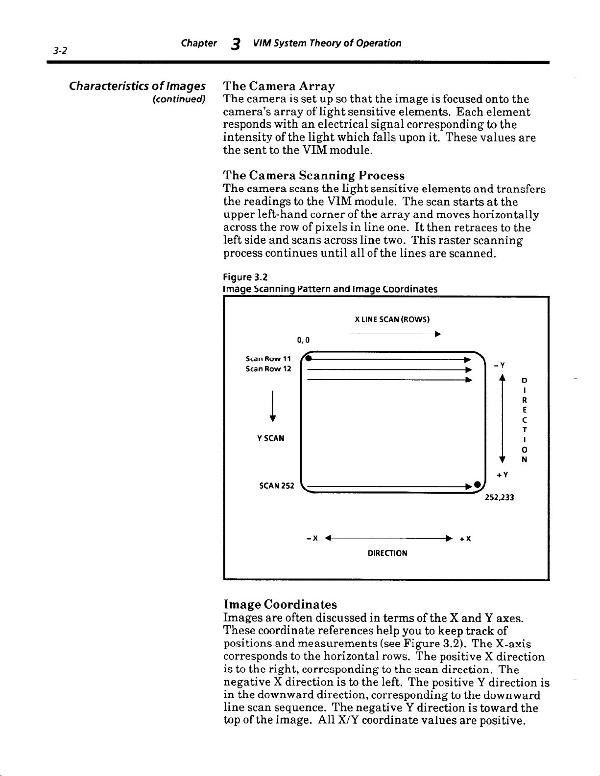
Characteristics of Images

(continued) The camera is set up so that the image is focused onto the

Chapter 3

The Camera Array

camera’s array of light sensitive elements. Each element
responds with an electrical signal corresponding to the
intensity of the light which falls upon it. These values are
the sent to the VIM module.

The Camera Scanning Process

The camera scans the light sensitive elements and transfers

the readings to the VIM module. The scan starts at the

upper left-hand corner of the array and moves horizontally

across the row of pixels in line one. It then retraces to the
left side and scans across line two. This raster scanning
process continues until all of the lines are scanned.

Figure 3.2

lmaae Scannina Pattern and lmaae Coordinates

VIM System Theory of Operation

X LINE SCAN (ROWS)

0.0

-

b

Scan Row 11

Scan Row 12

I
R
E

C

Y SCAN

1 0

SCAN 252

-x 4

DIRECTION

Image Coordinates

Images are often discussed in terms of the X and Y axes.
These coordinate references help you to keep track of

positions and measurements (see Figure 3.2). The X-axis
corresponds to the horizontal rows. The positive X direction
is to the right, corresponding to the scan direction. The
negative X direction is to the left. The positive Y direction is
in the downward direction, corresponding to the downward
line scan sequence. The negative Y direction is toward the
top of the image. All X/Y coordinate values are positive.

+ -Y

-be
252,233

b +x

0 D 1

I

N

+Y

Chapter

3 VIM System Theory of operation

3-3

Gray Levels

Each pixel in the image array generates an analog signal
that corresponds in strength to the brightness of the light.
The pixel output is converted to a digital value for use by the
digital computer system in the VIM module. This
conversion of the array’s analog signals into digital values is
known as analog to digital (A/D) conversion.

Gray- .Sca/e Conversion The analog signal is converted into a set of digital values

referred to as gray scale. This term refers to the fact that
the conversion process creates classifications for black pixel
values, through a wide range of gray values, all the way to
white. The gray scale is characterized by the number of
grays that quantified during A./D conversion, i.e., 256.

Let’s look at a simple example of how this works. An image
is collected and sent to the A/D converter. The converter is
designed to convert into four gray levels. In Figure 3.3, we
see that dark pixels are assigned a value of 0. Middle gray
values are assigned a value of 64 through 128.

Bright
values are assigned a value of 255. These gray levels
provide a measure of light intensity.

Figure 3.3
Four Craw Converted to Diaital Values

-

3-4

Chapter

3 VIM System Theory of Operation

The VIM Module

Gray Scale

The VIM module converts brightness to 256 gray values.
(This corresponds to the number of values that can be
encoded into 8-bits (1 byte)). This is sometimes referred to
as &bit gray scale. Images displayed in gray scale look like
black and white television images, with a wide range of
grays in the image. Figure 3.4 shows a gray-scale (analog)
image.

Figure 3.4

Grav-level (Analoa) lmaae

-

~h7dfh~~Ofl Of

Gray-Level Images

Binarization of images greatly reduces the complexity of the
image-processing tasks. The term “binary” refers to the two
states which may be given to a single bit of information:
black or white. These are ON (digital value of 1) and OFF

(digital value of 0). Using this technique, each pixel

requires only one bit of information.

A vision tool known as a threshold is used as a reference
value. Gray-scale values below or equal to the threshold are
converted to binary O’s (black) and values above the
threshold are converted to l’s (white). The resultant image
shows only black and white pixels.

__

Chapter 3 VIM System Theory of operation

Binarization of

Gray- Level hager

(continued)

3-5

Figure 3.5
Binarized lmaae With a Low Threshold

The threshold setting can alter the appearance of the image
substantially. As the threshold is increased, the image
becomes darker; more gray values fall below the threshold
and take on the 0 (black) value. As the threshold is
decreased, the image becomes lighter; more gray values fall
above the threshold and take on the 1 (white) value.

This difference in image appearance at different threshold
settings can be seen by comparing the different threshold
settings on the same image in Figures 3.5 and 3.6. The
higher threshold setting in image 3.6 creates a darker image
and affects the appearance of image features differently.

The thresholds provide flexibility to allow you to enhance

features of interest.

3-6

Chapter 3 VIM System Theory of Operation

Binarization of

Gray- Level Images

(continued)

Ire 3.6

Figu
Binarized image With a High Threshold

Setting Image Thresholds

The effective use of the thresholds requires that you

understand how to use them to create the best image for the
features you are analyzing. The objective of setting a

threshold is to get sharp contrast between the feature to be
measured and the surrounding area. In binary images, this
means that you need the feature of interest to be either
black or white and its surroundings to be the opposite value.

We’ll use two gray objects as an example. The object of

interest is light gray and the background upon which it is

located is dark gray. By setting the threshold at a gray
value that falls between the light and dark grays of the

object and background, the object appears as white and the

background appears as black.

If the threshold is too high, both object and background

appear black. If it is too low, both object and background

appear white. The VIM module provides you with four

images, each with its own threshold setting. During

operation, all four images are captured and processed

simultaneously. This creates the capability to set

thresholds to suit a range of image feature values.

Chapter 3 VIM System Theory of operation

Reading Threshold Values You’ll be able to judge the threshold setting best by

experimenting. View the results of threshold changes on

the monitor; however, if you would like to see the numeric

threshold value it can be read through the PLC

programming terminal.

A block transfer of the window configuration block is

required to read the actual threshold gray-level setting. For

more information of the use of block transfers, refer to

Chapter 5, “VIM Installation,” under the heading “PLC

Communications.”

Brightness Probe The brightness probe can be used to adjust for lighting

Lighting Compensation

variation and its effect on thresholding results. Changes in

lighting intensity create corresponding shifts in the gray-

scale values in the scene, This can create changes in the

images if the contrast in the scene is not great enough. The

brightness probe provides feedback on lighting variation

that is used to adjust the thresholds in proportion to the

lighting shift. This feature allows the VIM module to
maintain high accuracy while tolerating some lighting
variation.

3-7

The Probe Operation The probe is a tool which monitors the brightness in a small

The Probe Reference Patch

area in the image and compares it to a learned reference
value. If the value it finds is different than the nominal
value, the thresholds for the images are adjusted

accordingly. This is an optional function.

The probe samples a small rectangular area in the image.
The probe reading is the average brightness value for the
pixels within the sample area. Figure 3.7 shows the probe
positioned over an image.

Lighting compensation works best when a stable reference

patch is provided. The patch should be a white object in the

work stage that always falls within the image (see Figure

3.8). The reference patch must be illuminated by the same

lighting that falls upon the workpiece. In this way, lighting
variations that affect the image of the workpiece are
detected through brightness variations in the patch.

3-8

Chapter

The Probe Reference Patch

(continued)

3 VIM System Theory of Operation

Figure 3.7

The Probe as Seen in the Video Monitor Durina

-

Setuo

Figure 3.8

The Probe Reference Patch Seen in the Live Video lmaae

Chapter

3 VIM System Theory of operation

3-9

The Probe Reference Patch

(continued) used as the reference patch when using lighting

Line Gauges

It is recommended that you carefully prepare the object to be

compensation. Suitable materials for the patch include
white adhesive labels and white correction tape.

Line Gauges are used extensively in the VIM module. The
Line Gauges operate on any of the four binary images. The
basics of line gauge operation are reviewed here before
proceeding to the specific line gauge measurement tools.

Line Gauges operate by taking a predefined sample from a
row or column in the image. The line gauge is referred to as

a horizontal line gauge when taken from a row or as a

vertical line gauge when taken from a column.

Figure 3.9

ixels and Corresponding Digital Values

Row of Line Gauge Pixels &

Corresponding Digital Values

corresponding to the value of the pixels along the line. This

is illustrated by comparing pixel representations with their
corresponding values, as shown in Figure 3.9.

The Line Gauges operate by analyzing these strings of

binary bits. These strings can be used to: find blob edge
locations, blob widths, the number of edges, to count white
and black pixels, and to count numbers of blobs.

3-70

Chapter 3 VIM System Theory of Operation

Blobs

Blobs are clusters of pixels of the same value (black or
white). Blobs typically correspond to features in the image
that the line gauge crosses. Blob width is measured by the
number of pixels in the blob. Blobs can be measured for
either white pixel or black pixel blob groupings.

Blob edges are measured in row or column coordinates. This

is why it is important to fully understand pixels and the
screen coordinate system. Edges in horizontal line gauges
are expressed as column locations. Edges in vertical line
gauges are expressed as row locations. Edges are the row or
column location of the first pixel at the beginning of a blob.
Edges may be detected for either end of a blob.

Figure 3.10
Black and White “Blobs”

White

Blob Blob

White

line Gauge

Measurements

\

J

v

Black

Blob

The VIM module offers fifteen different line gauge
measurement and feature counting functions based on the

line gauge techniques. These are:

Edge Measurements, including:

- find left/top edge of largest blob

- find right/bottom edge of largest blob

- find left/top edge of left/top blob

- find right edge of right/bottom blob

Center Measurements, including:

- find center of largest blob

- find center of left/top blob

- find center of right/bottom blob

Width Measurements, including:

- width of the largest blob

- width of the left/top blob

- width of the right/bottom blob

Chapter

3 V/M System Theory of operation

3-17

­Line Gauge

Measurements - count white pixels

(continued)

Area Measurements, including:

- count black pixels

Blob Counts, including:

- count white blobs

- count black blobs

Edge Count

The measurement descriptions provided apply to both
horizontal and vertical line gauges. Vertical line gauges
read from top to bottom. Left/top blob and edge references

apply to both Left-most and top-most blob and edge.
Right/bottom blob and edge references apply to the right-

most and bottom-most blob and edge. Left and right edge

references apply to the top and bottom edges respectively.

Line Gauge The line gauge measurements are grouped into pairs. You

Measurement Pairs

may select one of nine different icons, each with a different
measurement pair. They are as follows:

Line Gauge Function One measures:

1) the left/top edge of the largest blob

2) the width of the largest blob

Line Gauge Function Two measures:

1) the right/bottom edge of the largest blob

2) the width of the largest blob

Line Gauge Function Three measures:

1) the center of the largest blob

2) the width of the largest blob

Line Gauge Function Four measures:

1) the left/top edge of the left/top blob

2) the width of the left/top blob

Line Gauge Function Five measures:

1) the center of the left/top blob

2) the width of the left/top blob

3-12

Chapter 3 VIM System Theory of Operation

Line Gauge

Measurement Pairs

(continued)

Line Gauge Function Six measures:

1) the right/bottom edge of the right/bottom blob

2) the width of the right/bottom blob

Line Gauge Function Seven measures:

1) the center of the right/bottom blob

2) the width of the right/bottom blob

Line Gauge Function Eight counts:

1) the number of white pixels

2) the number of black pixels

Line Gauge Function Nine counts:

1) the number of black or white blobs

2) the number of edges

Both measurements in a pair are active when they are

assigned to a line gauge. You should assign an acceptance
range to both of the measurements using the Line Hi/Lo
Range Menu. The acceptance range acts as a accept/reject
test of the measurement. Measurements that fall within the
acceptance range high and low limits are good.
Measurements that exceed these limits are “out-of-range”
and a REJECT decision is communicated.

Edge Measurements

The principles behind these line gauge measurement
techniques are explained in the following sections.

Edge measurements find the edges of blobs on the line, left
or right, top or bottom. The edge measurement is selected
by using the icon interface to scroll to the desired
measurement set. You read edge location settings by
identifying the location of the top arrow in the icon.

The icon displays a set of either two or three linear blobs.
The three blob set indicates measurements of the largest
blob -- indicated by the arrows pointing to features of the
largest blob in the icon (see Figure 3.11). The two-blob icon
indicates measurements of the left/top or right/bottom blob
(see Figure 3.12).

Figure 3.11

m-m

Line Gauge Function One
Measuring the Left/top Edge of the
Largest Blob

Chapter

Edge Measurements

(continued)

VIM System Theory of operation

3

Figure 3.12

Line Gauge Function Four
Measuring the Left/top Edge

of the Left/top Blob

3-73

The Edge Measurement Technique

A blob edge exists wherever two adjacent pixels have

different colors. So, blob edges are detected by a change in
pixel value from 0 to 1 or 1 to 0. Which change is read is
determined by the selection of either white or black blob
counting. If black blobs are selected, transitions from white
pixels to black blob strings are counted as edges (see Figure

3.13). The pixel which changes the value is read as a blob
edge. A single pixel may be read as a blob. In this case, both
edges would have the same value and the width would be

one (1).

Note: The edge location reported is that of the first (or last)
pixel of the color shown in the “Select Blob Color” icon. So,
for a blob that is one pixel wide, its left/top and right/bottom
edges are at the same position.

Figure 3.13

iges for a Black Blob

Blob Blob

Left Edge

Column Column

Value of 120

Right Edge

Value or 124

Single pixel blobs are sometimes due to noise in the image
(unwanted signals). The edge finding and blob finding
functions can adjust for this using line gauge filters. The
filters cause small blobs (one or two pixels wide) to be
ignored. See the “Line Gauge Filters” heading later in this
chapter for details.

3-74

Chapter 3

VIM System Theory of Operation

Edge Measurements

(continued)

Setting the Line Gauge Edge Finding Functions

The line gauge edge measurement functions are:

- find left/top edge of largest blob & largest blob width;

- find right/bottom edge of largest blob & largest blob
width;

- find left/top edge of left/top blob & left/top blob width;

- find right/bottom edge of right/bottom blob &
right/bottom blob width.

Set the function and size that suits your application. Leave
enough line off of the edge of the blob being measured to

allow for position variation and filtering (four to eight pixels
suggested).

Setting Hi/Lo Range Limits for Edges

Setting a range limit for an edge limits the amount of
position variation that is tolerated before a reject decision is
made. This tolerance is expressed in pixel counts, i.e., the
edge location may vary by four pixels in the positive
direction and four in the negative direction. There are three
steps to setting the range limit:

Step 1) Set the workpiece in the nominal (expected)

position and set the line gauge to the
appropriate size, location, and edge finding
setting. Select the edge finding measurement
in the Hi/Lo Range menu and take a reading of
the edge location.

Step 2) Determine the amount of variation that can be

tolerated in the positive ( + > direction (in

pixels) and add this value to the nominal
location value. Set the high range limit to this

value.

Note: One method to determine this value is to
move the workpiece as far right (or down) as it
will go. Use the edge reading at this position as
the high range limit.

Step 3) Determine the amount of variation that can be

tolerated in the negative ( - > direction (in

pixels) and subtract this value from the
nominal location value. Set the low range limit
to this value.

Note: One method to determine this value is to
move the workpiece as left (or up) as it will go.
Use the edge reading at this position as the low
range limit.

-

Chapter 3

V/M System Theory of operation

3-15

Edge Measurements

(continued)

A range of + /- 4 pixels might appear as:

116< =120< =124

Note: Edge range limits “float” when you use X/Y position
compensation. For example, when a horizontal line gauge
floats two pixels to the right, its high and low range limits

are both temporarily increased by two.

Center Measurements

Center measurements find the centers of blobs on the line.

The center measurement is selected by using the icon

interface to scroll to the desired measurement set. You read
center location settings by noting the location of the top
arrow in the icon. Center measurements are indicated by
downward pointing arrows that center on one of the blobs.

Figure 3.14
Line Gauge Function Three -

Measuring the Center of the

-

Largest Blob

Figure 3.15
Line Gauge Function Five -

Measuring the Center of the
Left/top Blob

The icon displays a set of either two or three linear blobs.
The three blob set indicates measurements of the largest
blob -- indicated by the arrows pointing to center of the

largest blob in the icon (see Figure 3.14). The two-blob icon
indicates center measurement of either the left/top blob or
right/bottom blob (see Figure 3.15).

Measurement Technique

Blob centers are measured by finding the center pixel in a
blob. Which blob is read is determined by the selection of
either white or black blob counting and the line gauge
function selected. If black blobs are selected, black blobs are
measured for center locations (see Figure 3.16).

Note: When the width of a blob is an odd number, the
central pixel position is reported as the blob center. When
the width is even, the pixel nearest position to the left of the
center is reported.

3-16

Chapter

Center Measurements

(continued)

3 VIM System Theory of Operation

Figure 3.16

Center for a Black Blob

I

Center of a

Black Blob

Column Value of 122

Setting the Line Gauge

The line gauge center measurement functions are:

- find the center of the largest blob & largest blob
width;

- find the center of the left/top blob & left/top blob
width;

- find the center of the right/bottom blob &

right/bottom blob width.

Set the function and size that suits you application. Leave
enough line on each side of the blob being measured to allow

for position variation and filtering (4 to 8 pixels is
suggested).

Setting Hi/Lo Range Limits

Setting a range limit for a blob center limits the amount of
position variation that is tolerated before a reject decision is
made. This tolerance is expressed in pixel counts, i.e., the
center location may vary by four pixels in the positive
direction and four in the negative direction. There are three
steps to setting the range limit:

Step 1) Place the workpiece in the nominal (expected)

position and set the line gauge to the

appropriate size, location, and center finding
setting. Select the center finding measurement
in the Hi/Lo Range menu and take a reading of
the center location.

tolerated in the positive ( + ) direction (in
pixels) and add this value to the nominal
location value. Set the high range limit to this
value.

- Step 2) Determine the amount of variation that can be

Chapter 3

VIM System Theory of operation

3-17

Center Measurements

(continued)

Width Measurements

Step 3) Determine the amount of variation that can be

tolerated in the negative ( - ) direction (in

pixels) and subtract this value from the

nominal location value. Set the low range limit
to this value.

A range of +/- 4 pixels for a nominal position of 120 appears

as:

116< =120< =124

Note: Center range limits “float” when you use X/Y

position compensation. For example, when a horizontal line
gauge floats two pixels to the right, its high and low range
limits are both temporarily increased by two.

Width Measurements find the width of blobs on the line.
The width measurement is selected by using the Line Gauge

Main Menu to select the desired measurement set. You read
width measurement settings by noting the location of the
bottom arrows in the icon. The arrows are located under the

blob being measured.

Figure 3.17
Line Gauge Function Two ­Measuring the Width of the
Largest Blob

1

Figure 3.18

Line Gauge Function Five -

Measuring the Width of the

Left/top Blob

The icon displays a set of either two or three blobs. The
three blob set indicates measurements of the width of the
largest blob -- indicated by the two-headed arrows
positioned under the largest blob in the icon (see Figure

3.17). The two blob icon indicates width measurement of the
left/top or right/bottom blob (see Figure 3.18).

Measurement Technique

Blob widths are measured by counting the number of pixels
in a blob. Which blob is measured is determined by the
selection of either white or black blob counting and by the
line gauge function selected. If black blobs are selected,
black blobs are measured for width (see Figure 3.19). A
single pixel may be read as a blob. In this case, the width
would be one pixel.

3-18

Chapter 3

V/M System Theory of Operation

Width Measurements

(continued)

Note: Minimum blob width when using Line Filter One is

two pixels. Minimum blob width when using Line Filter
Two is three pixels.

Figure 3.19

Width of a Black Blob
I

Width of a Black Blob

Pixel Count Value of 5

Setting the Line Gauge

The line gauge width measurement functions are:

- Find the width of the largest blob & left/top edge,
right/bottom edge, or center;

- find the width of the left/top blob & left/top edge or
center;

- find the width of the right/bottom blob & right/bottom
edge or center.

Set the function and size that suits your application. Leave
enough line off both edges of the blob being measured to
allow for position variation and filtering (4 to 8 pixels
suggested).

Setting Hi/Lo Range Limits

Setting a range limit for blob width limits the amount of
width variation that is tolerated before a reject decision is

made. This tolerance is expressed in pixels, i.e., the width is

permitted to vary by plus or minus four pixels. There are
three steps to setting a range limit.

Step 1) Place a workpiece that is the nominal size and

set the line gauge to the appropriate size,
location, and width measuring setting. Select
the width measurement in the Set Range menu
and take a reading of the blob width.

Step 2) Determine the amount of variation that can be

tolerated in additional width (in pixels) and

add this value to the nominal value. Set, the

high range limit to this value.

Chapter 3 VIM System Theory of operation

-

Width Measurements

(continued)

Note: one method of determining this value is

to find a workpiece that is barely acceptable.

3-19

Then set the high or low range limit to the
barely acceptable reading. Two workpieces
may be necessary: one that is almost too big
and one that is almost too small.

Step 3)

Determine the amount of variation that can be
tolerated less than the nominal width (in
pixels). Subtract this value from the nominal

value. Set the low range limit to this value.

Note: one method of determining this value is

to find a workpiece that is barely acceptable.

Then set the high or low range limit to the

barely acceptable reading. Two workpieces
may be necessary: one that is almost too big
and one that is almost too small.

A range of + or - 4 pixels for a nominal width of 20 pixels

appears as:

16< =20< =24

Count White/Black Pixels The Count White/Black Pixels function counts both the

black and white pixels on the line. This count is not related
to the number of blobs on the line. A line gauge which
counts pixels is like a long, thin window.

Setting the Line Gauge

Set the line size position that suits your application. Leave
enough line to accommodate workpiece position variation.

3-20

Chapter 3 VIM System Theory of Operation

Count Black/ White Pixels

(continued)

Setting Hi/Lo Range Limits

Setting a range limit for pixel counts limits the amount of
black or white pixel variation that is tolerated before a
reject decision is made. This tolerance is expressed in pixels,
i.e., the count, may vary by plus or minus four pixels. There
are three steps to setting the range limit.

Step 1)

Place a nominal workpiece in the workstage.

Select the Count White/Black Pixels

measurement in the Hi/Lo Range menu and

take a reading of the pixel count.

Step 2)

Determine the amount of variation that can be
tolerated in additional pixels and add this
value to the nominal count. Set, the high range
limit to this value.

Note: One method of determining this value is
to use the reading from a barely acceptable
workpiece.

Step 3)

Determine the amount of pixel variation that
can be tolerated less than the nominal count.
Subtract this value from the nominal value.
Set the low range limit to this value.

Note: One method of determining this value is
to use the reading from a barely acceptable
workpiece.

A range of + or - 10 pixels for a nominal count of 95 appears

as:

85< =95< =105

Count Number of Blobs The Count Number of Blobs function counts the black or the

white blobs on the line. This count is not related to any blob
features such as edges or widths. This function is useful, for
example, for counting the number of teeth on a comb.

Measurement Technique

The Count. Black/White blobs function counts the number of
black or white blobs on the line gauge. The blob color
counted is selected with the Select Blob Color icon.

Chapter

-

Count Number of Blobs

(continued) Set the line size position that suits your application. Leave

3 VIM System Theory of operation

Setting the Line Gauge

3-2 7

enough line to accommodate part position variation and
filtering.

Setting Range Limits

Setting a range limit for blob counts limits the amount of

blob count variation that is tolerated before a reject decision

is made. This tolerance is expressed in blobs, i.e., the count

may vary by plus or minus two blobs. There are three steps

to setting the range limit.

Step 1) Place a good workpiece on the workstage.

Select the Count Number of Blobs icon in the
Hi/Lo Range menu and take a reading of the
blob count.

Step 2) Determine the largest number of blobs that can

be tolerated. Set the high range limit to this
value.

Count Number of Edges

Step 3) Determine the least amount of blobs that can

be tolerated. Set the low range limit to this
value.

An acceptance range of + or - 2 blobs for a nominal count of

16 appears as:

14<=16<=18

The Count Number of Edges function counts the number of
blob edges on the line. This count is not affected by the
setting of the Blob Color icon.

This function is useful to measure the texture of the
workpiece. It measures how frilly or busy the surface is.

Bland workpieces give low number-of-edges readings.

Measurement Technique

The Count Number of Edges line gauge simply counts the

number of edge transitions (from black to white) in the line
gauge.

3-22

Chapter

3 VIM System Theory of Operation

Count Number of Edges

(continued)

Setting the Line Gauge
Set the line size position that suits your application. Leave
enough line to accommodate part position variation and
filtering.

Setting Hi/Lo Range Limits
Setting a range limit for edge counts limits the amount of
edge count variation that is tolerated before a reject decision
is made. This tolerance is expressed in edge counts, i.e., the
count may vary by plus or minus three edges. There are
three steps to setting the range limit.

Step 1)

Place a nominal part in the workstage. Select

the Count Number of Edges measurement in
the Set Range menu and take a reading of the
edge count.

Step 2)

Determine the amount of variation that can be
tolerated in additional edges and add this value
to the nominal count. Set the high range limit
to this value.

Step 3)

Determine the amount of edge count variation
that can be tolerated. Subtract this value from
the nominal count. Set the low range limit to
this value.

An acceptance range of + or - 3 for a nominal count of 15

appears as:

12< =15< =18

Using Line Gauge Filters Under some conditions, line gauge measurements may be

subject to interference or noise in the image. The Line Filter

function is used to remove this noise. Three line filter
settings are provided to adjust for varying degrees of noise.

Under low-contrast conditions you may see noise in the live
video image. It commonly appears as a “graininess” around
the edges of objects. Black pixels in white areas and white

pixels in black areas may be caused by noise. The filter

should be set to accommodate the level of noise in the image.

Filters can also be used to ignore fine detail in the image.

For example, you may be able to disregard the thin
decorative borderline around the edge of a label by using a

two-pixel filter.

Chapter 3 VIM System Theory of operation

3-23

Using Line Gauge Filters

(continued)

The Filtering Technique

The Line Filters work by comparing relationships between
groups of adjacent pixels on the line. A series of line
readings are used for illustration purposes. A line with two
large, black blobs might look like this:

1111000000000000111100000001111111111

-----

-----

zack Blob #T

*==j

Black Blob #2

Noise in the signal might appear as isolated pixels that do
not correspond to part characteristics. This creates small
signal variations which can be misinterpreted as blobs or
breaks between blobs.

1111000000001000111100000001111011001

t

? t

Unwanted variations.

Line Filter Zero

Line Filter Zero does not process the line to eliminate noise.
Line Filter Zero is actually a filter OFF setting.

Line Filter One

The line filter can be set to ignore these small variations by
removing them. Line Filter One disregards single-pixel
variations. When single-pixel filtering is selected, the line

would then be interpreted as:

1111000000000000111100000001111111001

t t

Single pixel noise filtered out.

Note: The dual-pixel noise on the right is not removed by
Line Filter One. Line Filter One requires a minimum of two
consecutive pixels to count a blob.

Line Filter Two

Line Filter Two ignores both one and two-pixel noise pulses.
The same line would then be interpreted as:

1111000000000000111100000001111111111

t

t t

One and two pixel noise filtered out.

Line Filter Two requires at minimum of three consecutive

-

pixels (of the selected color) to count a blob. The left/top­most pixel on the line is never filtered out. The second pixel
on the line is filtered out by Line Filter One if both of its
neighbors agree. Likewise, the third pixel is filtered out if
both of its neighbors agree. This three-pixel neighborhood
moves along until each pixel has been considered.

3-24

Chapter 3 VIM System Theory of Operation

X/Y Float Gauges

VI/id0 w Windows are area measurement tools. There is one window

Measurements

X/Y Float Gauges use the blob edge or center finding ability
of the VIM to detect variation in workpiece location. You
may use a blob center or edge to measure position variation.
These measurements are discussed earlier in this chapter.

The X and Y Float Gauges remember the nominal or normal
workpiece position and use the difference between the

nominal and the measured position to adjust the location of
the other (floating) line gauges and windows.

for each of the four thresholded images. You define the
window size and location. Each window may be setup to
measure either white or black areas.

Each window may also be set to float (for workpiece position
compensation).

Setting Windows Enable/Disable Window

The windows may be enabled and disabled individually at

the Window Main Menu.

Setting Window Shape

The windows may be set to many different shapes. This

includes: a rectangular window, a right angle triangle with
four possible orientations, a circular window, and a trained­through-the-lens mask.

Moving Windows

Windows may be moved anywhere within the image area.
The top 48 rows may not be used for windows if the

immediate brightness compensation mode is selected for the
brightness probe. The “train-through-the-lens” windows
cannot be moved.

Setting Window Size

Window sizes are individually adjusted horizontally and

vertically. The circle window adjusts in both directions
simultaneously. The “train-through-the-lens” windows
cannot be adjusted for size.

Chapter

VIM System Theory of operation

3

3-25

Counting Pixels

The windows operate by counting the number of pixels

(black or white) in the window. “Train-through-the-lens”

masks count pixels which lie under white areas of the mask.

Setting Hi/Lo Range Limits

Setting a range limit for windows limits the amount of black
or white pixel area variation that is tolerated before a reject
decision is made. This tolerance is expressed in pixels, i.e.,
the count may vary by plus or minus 50 pixels. There are
three steps to setting the range limit.

Step 1) Place a nominal workpiece in the workstage.

Take a reading of the pixel count in the

window.

Step 2) Determine the amount of variation that can be

tolerated in additional pixels and add this

value to the nominal count. Set the high range

limit to this value.

Note: One method of determining the high
limit is to use the reading from a workpiece

-

which is almost too big.

Step 3) Determine the amount of pixel variation that

can be tolerated less than the nominal count.

Subtract this value from the nominal value.
Set the low range limit to this value.

Note: One method of determining the low
limit is to use the reading from a workpiece

which is almost too small.

A range of + or - 50 pixels for a nominal count of 495
appears as:

445< =495< =545

-

3-26

Chapter

3 VIM System Theory of Operation

PLC Communications

Overview

Discrete Bit

Communications discrete I/O. VIM status is communicated for module

The VIM module communicates with the PLC systems

through discrete bit or block transfers. The Discrete bit
transfer sends one accept/reject signal to the PLC controller
at the completion of the inspection cycle. Block transfers
send the complete list of measurements and range alarms to

the PLC controller.

The VIM module communicates information through

failure, configuration faults, or module status. In addition,
alarms are communicated for Probe Range Alarm, X/Y
Float Range Alarm, and Master Range Alarm. The Master
Range Alarm communicates a decision failure if any of the
window, line gauge, or probe acceptance range tests fail.
Additional discrete bits are used to communicate trigger
signals, results block format, and to signal “busy” status.

Block Transfer

Block transfers communicate both numeric measurements

Communications and ACCEPT/REJECT bits for every vision tool.

Results Block

The detailed results of an image analysis are stored in a
“Results Block.” The Results Block is used to communicate
actual measurement data, as well as discrete accept/reject
signals, to the PLC controller. This includes:

- Individual tool range alarm bits

- brightness measurement

- pixel counts for each window

- two line gauge values for each line gauge

Configuration Blocks

The configuration data for a VIM setup may be transferred
to and from the PLC controller. These blocks of data are
referred to as the “Configuration Blocks.” They include
setup data such as:

- window size and location

- line gauge size, location, and function

- acceptance range high and low limits

- probe location and range limits

_-

Chapter 3 VIM System Theory of operation

Chapter Summary

3-27

This chapter has introduced you to some of the basics of
vision technology and demonstrated how these basics are

applied in the Vision Input Module. These basics include
vision image coordinates, gray-level image collection,

binarization of images, and setting binary thresholds.
These techniques help to understand the operating

principles of the vision tools used in the brightness probe,

line gauges and windows. Advice was provided on setting

acceptance range limits. Refer to this section should you

have any questions on the proper range limits as you set up
your application.

-

-

Chapter

4

-

Staging for

Vision Applications

Chapter Objectives

-

Successful vision applications are based upon good image

quality. Image quality is the result of proper illumination,
lens selection, and camera and lens setup. You should keep

in mind the first law of machine vision:

“Ifyou can’t see it clearly in the video monitor, then you

can’t inspect it with the vision system.”

In Chapter 3, we discussed the image-processing task of

converting light into images for processing by the VIM
module. In this chapter we will discuss the application of
lighting, cameras, and lenses to create quality images. This
process is called staging.

There are two main objectives in the design of a vision
workstage:

1) To make the features of interest clearly visible;

2) To reduce clutter in the image and eliminate
irrelevant features from the image.

This chapter discusses specific tools and techniques to

achieve these objectives.

Forming the Image

Focus

To use the VIM vision system effectively, a well-formed

image must be presented to the vision system. A well
formed image gives more precise and consistent

measurements. Two key elements that affect image quality

are focus and image contrast.

The collection of light through the camera lens is a critical
step in the formation of the image. The lens must be set at
the proper distance from the workpiece and then properly
focused. Lens focus determines the sharpness of the features
in the image.

Image features such as edges and thin sections must be

clearly focused to prevent a loss of clarity due to blurring.
Blurred images may change appearance as the binary
threshold levels are changed. This is because features like
edges may appear as blurred transitions from white to gray
to black and threshold changes move the apparent position

4-2

Chapter 4 Staging for Vision Applications

-

focus of the edge along with the changing gray level of the blurred

(continued) edge. This problem is not encountered when edges have

crisp contrast with no blurring.

Blurring can be caused by rapid motion in high-speed
applications. In this case, you can use a strobe light to stop
the action and eliminate the motion blurring.

Focus also impairs the ability to see small detail. Small
features may be blurred and lose the sharp definition
required for precision measurements.

If you wish to inspect features at different distances from the
camera, you may want to increase the depth of field (depth of
focus) of your lens. To do this, you narrow the aperture
(increase the F-stop setting), and add more light to the
workstage to compensate for the loss of brightness. You can
also restrict the depth of field to defocus a busy background.
In any case, experimentation is critically important.

Image Contrast

The importance of

lllumina tion

Image contrast is extremely important to the successful
application of the VIM module. An ideal contrast situation
can be created through the use of backlighting. Back­lighting illuminates the object from the rear. The workpiece
blocks the light and appears as a solid black silhouette
against a bright, white background. This distinct contrast
in gray scale, from the very dark object to the very bright
background, makes it very easy to set an acceptable
threshold and makes the vision system relatively
insensitive to small variations in light level. Features that
have only minor variation in gray-scale intensity (low
contrast) are more difficult to separate.

When setting up your application, try to create as much
crisp, well-focused contrast as possible between features of
interest and the background. This ensures that the
thresholds will be easily set and that consistent
measurements will be obtained.

We have seen that sharp focus and contrast are key
elements in image formation. Both of these elements are
highly dependent upon the lighting provided in the image
area, sometimes referred to as the “workstage.” Because
light is the medium used by the vision system to make
measurements, it is crucial that the illumination be
consistent.

Chapter 4 Staging for Vision Applications

4-3

The importance of

///urnha tion

(con tin ued)

You should design an illumination stage that best suits your
application. Evaluate the workpiece’s features, color and
reflectivity as well as the background in order to determine
which type of lighting works best.

The image collected is the result of direct and reflected light.
The camera “sees” only the light intensity; it does not see
color. The gray level of a feature in the workstage is
determined by the interaction of light and the surfaces of
objects in the workstage area. When light strikes a surface,
it can be absorbed, transmitted, or reflected.

l Absorbed Light

A red object appears red because all the light rays except
red are absorbed. Dark objects absorb a lot of light.
Light objects absorb very little light and reflect most of it
away.

l Transmitted Light

Light passes through many types of glasses and plastics.
The light path is often radically modified by this
transmission. This light is called transmitted light.

--

Figure 4.1
Specular and Diffuse Reflection

.ight source

Specular Reflection

Camera

0

0

0

0

4P

11

0.’

Specularly reflec

light ray (glare)

l Reflected Light

ted I

I
I
I
I

Diffuse Reflection

Camera

Diffusely reflected

light rays

Light that is not absorbed or transmitted is reflected.
The two types of reflected light are specular and diffuse,
and usually both types are present. A glossy magazine
cover exhibits both types of reflection. When held at a
certain angle, light is reflected directly into the reader’s
eyes (specular reflection), and the print cannot be

-

observed. When tilted slightly, the specular reflections
are directed away from the reader and the diffusely
reflected light allows the print to be observed. Figure 4.1
shows both types of reflection.

4-4

Chapter

4 Staging for Vision Applications

Different Types of

lllumina tion

Several types of illumination devices may be used with the
VIM module. Many of these may be ordered directly from
Allen-Bradley as accessories. See your local representative
for details.

1. Incandescent Lighting

Incandescent lamps are popular because they are
economical and their intensity is easily adjusted.
However, ordinary incandescent lamps have limitations
since they exhibit a constant degradation in light during
their operating life. Using a halogen light source results
in a more consistent light output.

2. Fluorescent Lighting

Fluorescent lamps produce less heat than incandescent

lamps yet produce the same amount of light. Some

fluorescent lamps, in multiple-lamp fixtures, provide

large, diffuse illumination. Circular fluorescent bulbs
are excellent for illuminating small objects. Some
fluorescent lamps flicker at a rate of 60 Hz. This is the
same rate as the video frame rate. This flicker may
cause some jitter in the image. This jitter is most
apparent in image areas such as edges.

3. Strobe Lamps

When an object is moving past the camera at high

speeds, a strobe lamp flash of light can “freeze” the
motion to create clear images. The strobe produces high
intensity light for a very short period of time. The
brightness of the strobe flash may vary from flash to
flash.

The timing of the flash must be synchronized so that the
workpiece is present when the camera scans the area.
The VIM module can trigger an accessory strobe light
through the swingarm.

Chapter 4 Staging for Vision Applications

4-s

Methods of Illumination

In addition to evaluating what type of illumination is most
appropriate, you must also determine the optimum
placement of the light source(s).

Illumination methods can be divided into two categories:

1. Direct Illumination (Backlighting)
Light travels directly from the source to the camera lens,

and is not reflected. The object is placed between the
light source and the lens, and a silhouette is produced.

This technique is often referred to as backlighting

because the illumination comes from in back of the
workpiece. Backlighting limits the type of features that
may be detected to edge features only. Features that fall
within the object edge areas cannot be detected.

2. Indirect Illumination (Front Lighting)

Light is reflected from the object to the camera lens
making surface features visible. This technique is often

referred to as front lighting. Front lighting allows you to
see normally visible features of the part and to make
distinctions based upon gray-level appearances. It may

also cast shadows or create reflections which may or may

not be useful.

Each of these illumination methods is discussed in the
following paragraphs.

Direct lllumina tion

.

Diffuse Backlighting

Camera

Q

-

Figure 4.2 shows an example of Diffuse Backlighting.

Figure 4.2
Example of Diffuse Backlighting

This popular form ofdirect illumination is useful when a high­contrast silhouette is required. Diffuse backlighting is similar
to a slide viewing table where the light is behind a translucent
diffusing surface. This is the most easily constructed of all
backlighting methods. This approach works especially well
with flat workpieces; a well defined silhouette is produced.

4-6

Chapter 4 Staging for Vision Applications

Indirect lh~~ination Indirect Illumination, or front lighting, is used when surface

Front Lighting - Directed Bright Field

Front Lighting - Diffuse Reflection

I I

450

0

­features must be inspected. It’s also used when backlighting
is impractical. Figure 4.3 illustrates several examples of
Indirect Illumination.

Figure 4.3
Examples of Indirect Illumination

Directed bright field lighting places the camera near the angle
of reflected light. This is the area of brightest intensity in most
cases. This is particularly true of highly reflective parts with
glossy surfaces or light colors.

The shadows cast by bright field lighting may be used to create
strong contrast between a feature in the workstage and its
shadow. Use directed lighting to create strong contrast
between features of interest and their background areas.

Diffuse reflection is usually preferred to directed bright field
lighting because it offers a wider range of gray values for image
analysis. This is because the image is the result of the light
absorbing and diffusing qualities of the features, not the
reflecting qualities.

u

//

Front Lighting - Directed Dark Field

Q

A commonly used method is to place the illumination source at
45 degrees to the workpiece surface and the camera viewing
angle, assuming the camera is perpendicular to the surface.

Directed dark field is a side lighting technique where the angle
of illumination (angle of incidence) is very shallow. A very

small amount of the diffusely reflected light reaches the
camera, and the surface appears dark. Any abrupt change in

surface height causes a bright reflection into the camera’s lens,

often with an accompanying dark shadow next to it. Surface

flaws such as scratches and bumps are often detected using this

technique.

Bright Field Front Lighting

The image is greatly impacted by the angular relationship
of the lighting and camera. This is because most reflected

light bounces off of a surface at an angle equal to the angle

of incidence (angle of approach). The camera lens collects

the most light if its angle of incidence is along the axis of the

Chapter 4 Staging for Vision Applications

4-7

Indirect lllumina tion reflected light. This bright reflection creates a bright image

(continued)

in the camera field of view and is referred to as “Bright
Field” lighting (as shown in Figure 4.3). Bright Field
lighting often produces glare which may or may not be
useful.

Diffuse Front Lighting
Diffuse lighting moves the camera out of the main reflected
beam to collect the secondary light that is diffused
(scattered) by the object surface. The angle is enough to
reduce glare and still catch strong illumination from the
diffused light.

Dark Field Front Lighting
Dark field lighting places the camera at such an extreme
angle, away from the angle of reflection, that very little
light is reflected or diffused to the camera and a dark image
is formed. Directed dark field lighting is often used to
highlight surface variations such as scratches and pits.

Backdrops
You can often create high contrast between the workpiece

-

and its background simply by providing an appropriate
backdrop. For example, a medium gray object appears light
against a black background and dark against a white
background. You can also place the backdrop far enough
from the workpiece that it is out of focus enough to eliminate
clutter.

Lens Selection

and Adjustment

Another factor in quality image formation is lens
selection and use. The lens projects the image of the
workstage into the camera and onto the image collection
electronics (the image array). The lens must form a sharp,
even, undistorted image for consistent measurements to be
achieved. A brief discussion of the subject is presented here.

How a fens Works

Lenses bend light rays as they move from air into glass and
then emerge from the glass into the air. (The degree the
light rays bend depends on the angle of incidence and the
indices of refraction for glass and air.) Figure 4.4 shows two
simple lenses focusing light onto the image plane. In solid­state video cameras, the image plane is a photosensitive
array on an integrated circuit. A broad selection of lenses is
available to meet a variety of application requirements.

Chapter 4 Staging for Vision Applications

How a Lens Works

(continued) Lens selection is largely determined by the Field of View

Field of View

Field of View

required to see the full area of interest in the work stage.
Allow room for variation in part position unless the
workpiece is accurately fixtured.

The field of view is the area (field) seen by the camera and
projected onto the image array when the image is in focus.
There may be several lenses capable of meeting your field of
view requirements. Each of the lenses has a different

standoff distance.

Figure 4.4
Relationship of the Focal Length of a Lens to
Standoff Distance Given a Constant Field of View

Both Workstages
Have the Same Field of
View

Short Focal Distance (f) With Short Standoff - 12.5mm Lens

Standoff Distance

Longer Focal Distance(f) With Longer Standoff - 25mm Lens

Standoff Distance

Lens Extension Tube

*I-f4

Lens

I I- Im2f-m

Chapter 4 Staging for Vision Applications

How a Lens Works Lens Standoff Distance From the Workpiece

(continued)

Standoff is the ideal distance between the lens and the item
being inspected. The standoff for a given field of view is
determined by the fixed array size and the focal length of the
lens. The focal length is the distance between the lens
center and the image plane (image array in this case) when
objects in the field of view are in focus. Lenses are measured
by their focal length. A lens with a short focal length, such
as a 12.5 mm lens, has a shorter standoff for a given field of
view than a 25 mm lens. This is illustrated in Figure 4.4

The camera should be mounted far enough away so that it

does not interfere with the process or with the workstage
lighting. Other considerations might include keeping away
from parts that are hot or that emit vapors or dust; all of
which degrade the performance of the system.

Figure 4.5
Control of Light Collection Using the F-stop of the Lens

4-9

Aperture stopped down to decrease brightness

Iris

0

Aperture

Aperture

Lens Front View

Aperture opened to increase brightness

Lens Section View

4-10

Chapter 4 Staging for Vision Applications

-

How a Lens Works Lens Aperture (F-stop) Settings

(continued) You may control the amount of light collected by the lens

using an internal lens device called the F-stop. The F-stop
acts much like the pupil of your eye, controlling the amount
of light that comes in contact with the lens.

The smaller the aperture (opening), the less light that

enters the camera. Proper F-stop setting is very important

to image collection. Use the F-stop to control image

exposure and obtain the best possible contrast after the lens
has been focused (see Figure 4.5).

The F-stop number indicates the amount of light that passes
through the lens aperture. Care must be taken to remember

that as the F-stop setting increases, the brightness of the
image decreases. A typical set of lens F-stop values is 2.8,4,

5.6,8,11, and 16. The 2.8 setting collects the greatest
amount of light and the 16 setting collects the least amount
of light. For each step up in F-stop value (e.g., going from

2.8 to 41, the image brightness decreases by l/2.

Selecting the Lens for

Your Application

Note: Always switch the monitor display to the live analog
image before adjusting the camera focus or F-stop. To do
this, touch the Light pen to the top portion of the display
screen until the live analog image appears.

The following instructions aid you in the selection and
setup of lenses to suit your applications.

l Determine the required field-of-view

The field-of-view (FOV) is the area that the camera
“sees.” It should include every feature of the workpiece
to be inspected. Take into consideration any variation in
workpiece position that might move features of interest
out of the FOV and set your FOV size to accommodate it.

Note: The image array in the camera has an aspect ratio
of approximately 3 to 4. This means that the X-axis of
the image is longer than the Y-axis. The Y-axis is
approximately 75% of the length of the X-axis (see
Figure 4.6).

_-

Chapter 4 Staging for Vision Applications

4-77

Selecting the Lens for

Your Application

(con timed)

Figure 4.6

Aswct Ratio

3:4 Aspect

Ratio

Y=3

l Determine the Standoff Distance

4

x=4

Determine your ideal camera and lens standoff (distance
away) from the part. This is often dictated by a clearance
requirement to stay out of the way of moving machinery
or workpieces. Sometimes it is limited by available floor
space or ceiling height, or by a requirement to shroud the
workstage. It might also be the standoff distance that is
simply the most convenient for setup and maintenance.

*

l Determine Accuracy

Determine the accuracy to which the object must be
measured.

l Determine the Need for Extension Tubes

Some lenses need an extension tube to focus at close
distances. The extension tube is placed between the
camera and lens. If an extension tube is needed at a

given standoff distance, the length of the tube is listed on

the chart next to the distance to the object in Table 4.A.

Note: There are techniques for folding and enlarging the

standoff distance. For example, the camera can view the
workstage through a mirror or prism. This allows
considerable freedom in camera placement and angle.

4- 72

Chapter

4 Staging for Vision Applications

Using the Lens Reference table 4.A has been provided to aid you in the

Selection Tab/e

selection of the best lens for your application. You may use
the table based upon a known FOV or a desired accuracy.

Lens Selection if

FOIlis Known

Lens Selection if

Accuracy is Known

To use the LENS SELECTION TABLE in Table 4.A, if the
FOV is known, find the FOV (listed in the first column of the
table) that is larger than the FOV required by the

application. The FOV column lists the height, then width,

for FOVs from 0.3 to 32 inches in size

On the right side of the table, the standoff distance for each
lens that is recommended is shown for each FOV. The
preferred lens is indicated in bold type, and should be used
unless the physical constraints of the application limit the
choice of standoff distances. The second column of the table
gives the accuracy to which an object will be measured at
each FOV. The third column gives the pixel size.

To use the LENS SELECTION TABLE if the desired

accuracy of the measurement is known, find the desired

accuracy listed in the second column of the table. The
required FOV is listed in the first column, and the lens
standoff distance is listed in the right columns.

Lens and Camera

Set-up

When mounting your camera and lens assembly, set the

front of the lens at the standoff distance listed in the table
for your field of view. This distance is an approximation; it
will get your camera close to the ideal location. From there,
focus the lens and set the F-stop to get the proper clarity and
brightness.

Example One

The desired FOV is 3 by 4 inches. Using the table, the

preferred lens is 55mm, with a standoff distance of 26
inches.

Example Two

The desired accuracy of measurement is l/16 of an inch, or

0.063 inch. The closest value in the Table is 0.052 by 0.062

with an FOV of 4 by 5.3 inches. The preferred lens size is

25mm, using a lmm extension tube. The standoff distance

is 15.5 inches.

Chapter

Lens and Camera

Set-up

(continued)

I I

4 Staging for Vision Applications

Table 4.A

Lens Selection Table

I

I

4-73

105mm

2801-NL4

Height 1 Width

-+ 5.0 5.5 6.7 7.3

1 Height / Width

0.064 0.071 0.079 0.086

1 Height 1

0.022 0.024 0.026 0.029

Width /

92” 9” None +mm 19+* 21”

‘:ci-

None None

Dist.

to

Obj.*

21”

3%”

4”
5”

6+”

$3+”

lo;”

12;” *

15”

171”

20;” 41”

23”
26” 52”

29+” 59”

34”

39”

43” 86”

47”
51” -

to Obj. sion

h-

1

2

I I

Dist. Exten-

8;”

94”

1lG”
14;”

18”

21 ”

26”’

31”

36”

46”

68”

77”

94”

7” 40mm

1Omm

None
None
None
None
None
None
None
None
None
None
None
None
None
None
None
None

-

24 3;’

1 0 331 0 375

0.103 0 125

45” None 91”

None

No extension tubes are required with the 55mm lens. This lens is recommer

applications.

68” - -

77” - -

86” - -

-

-

-

-

ed for most

4- 14

Chapter 4 Staging for Vision Applications

Object Positioning

Still Objects If the workpiece can be inspected while it is still (not

The presentation of the object to be inspected by the VIM
module can be divided into one of two categories:

The object will be stopped in front of the camera, or

1)
The object will be moving.

2)

moving), the application will be easier to set-up. The
optimum set-up would position the object in front of a
camera, with a repeatability of better than one percent of
the FOV. For example, in a FOV of three by four inches, the
object would be positioned to within l/32 of an inch. If the
object cannot be positioned accurately, the VIM tools allow
adjustment for position variations. It is desirable to fixture
the object so that the variation in object location will be less
than 25% of the FOV. (Note that the use of these tools
slightly increases the time required to inspect each object.)

When the FOV for the application is calculated, the amount
of object positional variation must be added to the size of the
object inspection area to determine the FOV. For example,
an object that is two by three inches and positioned to within
one-half inch will require an FOV of 2-l/2 by 3-l/2 inches.

Moving Objects

For objects that are moving past the camera, a different set­up is required. If the object is moving, a strobe light is
probably needed to “freeze” the object’s motion in order to
eliminate blur in the image. A strobe light is set-up in the
same manner as a fluorescent or incandescent light. The
VIM module will trigger the strobe light at the correct time.
The strobe light trigger is connected to the VIM swingarm.

In order for the strobe light to eliminate blur in the image, it
must be much brighter than the ambient lighting. A cover
or shroud is often needed around the workstage to reduce
the ambient light. The shroud also prevents the flashing
strobe light from becoming a distraction to nearby workers.

To determine whether a strobe light is needed, calculate the
FOV necessary for the inspection, and find the size of a pixel
for that FOV using the Lens Selection Table. Divide the

Chapter 4 Staging for Vision Applications

4-15

Moving Objects

(con timed) is greater than one-half the pixel size, a strobe light should

speed of the object in inches per second by sixty. If the result

be used.

0

Example

The object is a ring with a diameter of three inches moving

at a speed of thirty feet per minute (six inches per second).
From the LENS SELECTION TABLE, select an FOV of
three by four inches. The pixel size is 0.013 inch by 0.016
inch. The object will move 0.1 inch (6 inches per second/60).

This is greater than one-half the pixel; therefore, a strobe

light is needed. The object speed would have to be reduced to
less than two feet per minute to eliminate the need for a
strobe light.

Using Filters With Filters are devices used to suppress interference which

the V/M Module

would appear as noise in an image. Lens and Illumination
filters may be used in a VIM module application situation.

Lens filters A colored lens filter can be useful in an application situation

that requires a certain colored item to stand out. If you are
inspecting shiny, transparent, or translucent workpieces,
polarizing filters can be valuable. Neutral density filters
can be used to restrict the focus or depth of field of a lens
setup. Use an infrared pass or cut filters if your workpiece is
heated or if you with to exclude ambient visible light.

Photographers have used lens filters for more than a
century. The techniques they have developed are all
applicable to machine vision. The bibliography in Appendix
D contains several references for photographic filter
techniques

lllumina tion Filters Illumination filters can also be used, or a combination of

illumination and lens filters can be used. For example, you
can illuminate a fluorescent workpiece with ultraviolet

light and observe the visible light it gives off. You can also
illuminate the workpiece with horizontally polarized light
and view through a vertical polarizing filter. The 2805
N13A Ring Polarizer and 2803-N13 Ring Light make dual
polarization a popular technique.

4-16

Chapter 4 Staging for Vision Applications

Workstage Shielding

-

To control contrast and shadows you need to enclose
(shroud) the workstage. This prevents stray reflections and
shadows from interfering with the automatic operation of
your system. Shrouding also provides a dark black
background which always increases the contrast.

It is also good practice to have any fixtures close to the
workstage finished in a flat black color. This prevents
reflections and the resulting uneven illumination. This is
the reason that camera lenses are black.

Chapter

5

lnstalla tion
and Integration

Chapter Objectives

In this chapter, we will acquaint you with the installation of
the VIM system. We will also provide guidelines for
integration into PLC systems and your process.

Integration of This section discusses, in detail, the installation and

VIM Components

Requirements for

installation In to an Existing is dependent upon two variables: availability of slot space

PLC 1771 II0 Rack

integration of the VIM module and its components.

Installation of a VIM module into an existing PLC I/O rack

and availability of sufficient power.

Availability of Space

The VIM module requires a module group (two adjacent
vacant slots) in which to be mounted. If your existing PLC

1771 I/O rack does not have two adjacent empty slots you
cannot install a VIM module. If this is the case, you have
two options:

1) acquire a larger rack;

2) acquire an additional rack.

See your local Allen-Bradley representative for details.

Availability of Sufficient Power

If your existing PLC I/O rack has the required space, your

next step is to determine whether the existing power supply
has enough current to satisfy the VIM module. The VIM

module requires 3 Amps of current (maximum) in order to

operate. Each module in the rack uses a portion of the
available current supply. To determine if your power source
has sufficient current, subtract the total amount of current

consumed by each individual component (see individual unit
documentation) from the total amount of current output
from your power source (see Power Supply documentation).
If the resultant number is greater than or equal to 3 amps,

sufficient current is available.

Total Current Output - Total Current Consumed = Available Current

If your z/O rack meets the above requirements you are ready

to install your VIM module (see the “VIM Module

Installation” section of this document).

5-2

Chapter

5 installation and Integration

Requirements for

Installation Into a 1771

Standalone /IO Rack

i/O Rack instalia tion

Power Supply instaIiation

A standalone I/O rack (such as catalog number 1771-PSC)
has four slots, two for the VIM module and two for an in­rack power supply (catalog number 1771-P3). Since the
standalone unit is self-contained, there will always be
enough space and current. For additional information refer
to the documentation accompanying your standalone rack.

For information on I/O rack installation, see documents

1771-4.5, “Mounting Instructions for 1771 I/O Chassis and
Power Supply,” and 1770-4.1 “Grounding and Wiring
Guidelines.” These documents must be read before
attempting installation.

Many PLC system power supplies are available for use by

the VIM module. For information on the installation of

specific power supplies, refer to the documentation

accompanying that power supply as well as Cat. No. 1770-

4.1, “Grounding and Wiring Guidelines.”

-

VIM Module instalia tion

This section describes the installation procedures for the

VIM module.

Keying Band Installation

Keying Bands are shipped with each I/O chassis. Each

backplane socket should be keyed to accept only the

designated type of I/O module (in this case the VIM module)

assigned to that slot. Keying guards against the wrong

module being installed in the wrong I/O rack slot.

Each VIM module plugs in to four sockets on the backplane

(two per slot). Keying bands are installed on the top right
socket. The socket has guide numbers along the right side to
aid in the positioning of the keying bands. Keying band
locations for the VIM module are between numbers 16 - 18
and 26 - 28 (see Figure 5.1).

Keying bands may be installed with needle-nose pliers and

are easily replaced.

-

Chapter

5 Installation and Integration

5-3

-

VIM Module Installation

(con timed)

Figure 5.1

Keying
Bands

-

Backplal
Socket

Setting the I/O Chassis Configuration Plug

Many 1771 I/O chassis contain a “configuration plug”. This

is a stake-pin jumper located on the chassis backplane near
the PLC controller slot. Set the configuration plug to the
right position (N) if you use an external chassis power
supply such as 1771-Pl. Set the configuration plug to the
left position (Y) if you use a power-supply module such as

1771-P4.

Set to Y when either: (Refer to Figure 5.2)

-

You are using an in-rack power supply module, or:

-

You are using VIM modules in the chassis in standalone

-

mode -- with no PLC processor present.

Set to N when:

-

Both an external power supply and a PLC controller are
used.

5-4

VIM Module lnstalla tion

(con tin oed)

Chapter

5 Ins tala tion and Integration

Figure 5.2

ings

Using Power
Supply Module
in this Chassis?

Module Installation

Open the module locking latch (see Figure 5.3) to insert the

module. Plastic guides, on the top and bottom of each slot,

permit the module to be easily slid into the rack (see Figure

5.3). Do not force the module into its backplane socket.

Apply firm and even pressure to seat it firmly into its

sockets.
After the VIM module is installed, secure it in its place with

the module locking latch (see Figure 5.3). After the module
has been properly seated and locked into place, its
Swingarm can be attached (see Swingarm section of this
chapter).

Chapter

VIM Module lnstalla tion

(continued)

5 Ins talla tion and lntegra tion

5-5

Figure 5.3
installation of the VIM Module

Camera Component

lnstalla tion

This section describes installation procedures for the video
camera, cable, lens, and extension tube. Figure 5.4 provides
a graphical illustration of camera component
configurations.

Connector Cable

The video camera, Cat. No. 2801-YB, is attached to the VIM
module by a la-pin connector cable: 2801-NC4(2M); 2810­NC5(5M); 2801-NC6(10M); or 2801-NC7(25M).

To connect the camera cable:

1) Identify the male and female ends of the cable

2) Plug the male end of the cable into the camera input
jack located on the face of the module (see Figure 5.5)

3) Plug the remaining female end of the cable into the 12-

pin output jack located on the back of the camera (see
Figure 5.6, Camera I/O Locations).

5-6

Chapter

Camera Component

lnstalla tion

(continued)

VIDEO CAMERA

Ins talla tion and lntegra tion

5

Figure 5.4
fnmwn Cnnfinuratinnc

C - MOUNT LENS

---

_~.~_~,~.~.~.~,~.~,~.~.~.~.~.~.~.
_~.~_~.~.~,~.~.~.~.~.~.~.~.~.~.~.
_~.~_~.~.~,~.~,~,~,~.~,~.~.~.~,~.

---

.~.~.~.~,~,~.~.~.~.~.~.~.~.~.~...

----

VIDEO CAMERA

EXTENSION TUBE
2801 - Nl
(OPTIONAL)

PHOTOGRAPHIC LENS

EXTENSION TUBE
2801 - Nl
(OPTIONAL)

C - MOUNT LENS
2801- NLl(25 mm)
2801 - NL2 (12.5 mm)
2801- NL5 (12 - 75 mm Zoom)

C-MOUNTTO
PHOTOGRAPHIC

2801 - NL3 (105 mm)
2801 - NL4 (55mm)

Chapter

Camera Component

/nstaIlation

(con timed)

Light Pen

Jack

5

installation and Integration

Figure 5.5

Front Panel Features

5-7

Status LED’s

Monitor

Connection

Camera

Connection

Swingarm
Field Wiring
Terminals

5-8

Chapter

Camera Component

/nsta//a tion

(continued)

5 installation and Integration

-

Figure 5.6

Camera I/O Locations

Camera Rear View

/

Video Out -­No Connections

DC In/Ext. Svnc. -­Insert Female End of
Connector Cable

The connectors or plugs should easily fit into their
respective jacks. If resistance is encountered realign the
pins and try again.

To remove the camera cable, reverse the above steps.
However, to unlock the cable from its connection, slide the
collar of the connector back towards you while pulling the
cable out of its jack.

Lenses

When you receive your video camera it will not have a lens.

You have the option of ordering any of the following lenses

depending upon your needs and applications:

2801-NLl, 25mm - C mount;

2801-NL2,12.5 mm - C mount;

2801-NL3,55 mm - Photographic, requires 2801-N2 Lens
Mount Adapter;

2801-NL4,105 mm - Photographic requires 2801-N2 Lens
Mount Adapter;

2801-NL5,12.5 to 75 mm - Zoom, requires 2801-N2 Lens
Mount Adapter.

Chapter 5 Installation and lntegration

5-9

Camera Component

lnstalla tion

(con timed) requirements and applications refer to Chapter 4, “Staging

See Figure 5.4 for an illustration of camera and lens
configurations. For information on typical lens

for Vision Applications.”

All lenses include an installation and maintenance
instruction booklet. Consult your local Allen-Bradley
representative for additional information.

Camera Extension Tube

The optional camera extension tubes are used to alter the

image focal length. This allows you to use the lenses at

shorter distances. See Chapter 4 “Staging for Vision
Applications.” Installation instructions are provided with
each unit (see Figure 5.4).

VIM Power Supply

VIM 12 Volt power is supplied by an external power supply

(Cat. No. 2803-Pl). Power supply terminals 4 and 5 are

wired to 117VAC. Power supply terminal 1 is connected to

swingarm terminal 1, and power supply terminal 2 is
connected swingarm terminal 2. Terminal 3 is connected to

ground. The power supply provides enough power for two

VIM modules.

The VIM power supply (Figure 5.7) provides the power used

by the camera.

Figure 5.7
VIM Power SUPPIV

S-10

Chapter

5 Installation and Integration

Camera Component

Installation

(continued)

WARNING: Remove system power before
attempting installation. Failure to do so may
result in electrical shock.

Light Pen lnstaiia tion The light pen (Cat. No. 2801-N7) is attached in the same

manner as a home telephone. Align the clear plastic plug,
located on the end of the light pen cord, with the light pen
input jack, located on the face of the VIM module (see Figure

5.5). If resistance is encountered check the alignment, the
release tab may not be properly seated in the slot.

To remove the light pen, press the release tab while pulling
the plug out of the jack.

Video Monitor lnstaiiation The monochrome video monitor (Cat. Nos. 2801-N6,12 inch

and 2801-N9,9 inch) is connected to the VIM module by a
BNC type coaxial cable (Cat. No. 2801-NC2 (5M) or 2801­NC3 (10M)). The video output jack is located on the front

panel of the VIM module. The video input jack is located on

the rear panel of the video monitor (see Figures 5.8, and 2.9,

12 inch monitor).

Figure 5.8
12 Inch Monitor

-

Chapter

5 lnstalation and integration

5-11

Video Monitor lnstalla tion

(continued) your video monitor. The screen can interfere with the

Note: Remove the plastic screen cover that comes with/on

operation of your light pen.

To connect the video monitor to the VIM module:

1) Locate the video input jack on the rear panel of the
monitor (Figure 2.9). Plug in one end of the coaxial
cable by aligning the slot, found on the connector, with
the cylindrical keys, found on the outside of the input

jack. Twist clockwise to lock (counterclockwise to

unlock).

2) Locate the video output jack on the face of the VIM
module (see Figure 5.5) and plug in the other end of the
coaxial cable.

To disconnect the video monitor, reverse the above steps.

The scan switch on the front panel of the monitor should be

set to “underscan.” This allows you to see all the way to the
edges of the image. The Brightness and Contrast controls
should be set for normal viewing. If set too dim, the light
pen will not be able to pick. If too bright, the wrong icon

may be picked.

Strobe Light

Connection

Swingarm

Swingarm Connections

The Strobe light trigger input is wired to Swingarm

terminals 5 and 6. For additional installation information,
refer to the manufacturer’s guidelines.

This section describes the Swingarm I/O connection device.
Each individual Swingarm connection is discussed as well

as the installation procedures for the Swingarm itself

Shielded cables reduce susceptibility to electrical noise and

interference and are highly recommended for use on all I/O

connected to the swingarm.

The Swingarm (see Figure 5.10) is a detachable I/O
connection device. This convenience enables you to remove
or replace modules from your I/O rack without having to
rewire the connections.

5-72

Swingarm Connections

Chapter

(continued)

5 Installation and Integration

Figure 5.9

wingarm - Field Wiring Terminals

Terminal Function

1
2
3 1 Trigger +24VDC Input
4

5
6 Strobe Common

7 1 Decision Output
8 1 Decision Common

9 1 Busy Output

10

11

12 1 No Connection
Use With 1771 -WB Wiring Arm

A

Camera Power Input
Camera Power Common

--

I

1 Trigger Common

Strobe + 5V TTL Output

Busy Common
No Connection

WARNING: Remove system power before

t

0

attempting installation. Failure to do so may
result in electrical shock. Do not use the Busy
output to directly energize external equipment.
the Busy output is energized during power-up

and reset to indicate that the module is not yet.
ready to perform an inspection.

Actual Swingarm connection assignments are illustrated in
figure 5.9; the following list describes each connection:

12 Volt Power Input (Cat. No. 2803-Pl) - Provides a

connection for the external power supply at terminals 1

and 2.

Trigger Input - Swingarm terminals 3 and 4 are used for
connections to sensors or other triggering devices. Your
Trigger Input signal must be from + 3.3 to 32 VDC. You
may use a pushbutton trigger device - see Figure 5.21.

Chapter

5 Ins talla tion and Integration

5-13

Swingarm Connections

(continued)

Strobe Light Output -Provides a connection for a 5 volt
TTL Strobe light (positive edge) trigger at terminals 5 and 6.
The Strobe light cable must be of shielded type and
terminated to at least 7.5 ohms. Shielded cables reduce
noise and interference and are highly recommended.

Decision Output - Swingarm terminals 7 and 8 are used
for output connections. The Decision Output will toggle
ON/OFF as a result of the ACCEPT/REJECT analysis.
This is an open-collector transistor type output, rated for 3
to 32 VDC, 1 ampere. ACCEPT = LED OFF, high
impedance. REJECT = LED ON, low impedance to
common.

Busy Output-The Busy signal indicates that the module
is busy and a decision is pending. It comes on as soon as
the “Trigger” has been received and goes off after
“Trigger” has been reset and “Decision” is set/reset. This
is an open-collector transistor type output, rated for 3 to
32 VDC, 1 ampere. “BUSY” status = low impedance to
common and LED ON. “NOT BUSY” or “READY” status

= high impedance and LED OFF.

Swingarm lnstaI/ation A Swingarm is required to operate the VIM module. The

lower end of the Swingarm forms a C-shaped bracket which

snaps onto the horizontal bar of the I/O chassis (see Figure

5.10). The Swingarm pivots upward and snaps onto the

front connector edge of the VIM module (see Figure 5.11).

Figure 5.10
Installation of the

Swingarm

5-74

Chapter

Swingarm Installation The Swingarm is removed by lifting the release tab located

(con timed)

5

installation and Integration

at the top of the Swingarm, just above the first terminal.

Figure 5.11

Swinaarm

Latch Connection

Note: The Swingarm release tab requires a fair amount of
pressure. Be careful not to press the tab too hard because
damage may occur.

Grounding Sufficient and proper grounding is extremely important to

Considerations

the performance of your VIM module. Your images will
show signs of interference or noise if the system is
improperly grounded. Noise is due to electromagnetic and

electrostatic interference and is eliminated by proper earth

grounding.

CAUTION: Ground loops can seriously impair

t

0

A

the performance of the VIM module. Ensure that
proper grounding procedures are followed. Refer
to Cat. No. 1770-4.1, “Grounding and Wiring
Guidelines” for correct grounding procedures.

Chapter

5 Installation and lntegration

s-15

lndica tor Lights

(LED’s) (Light Emitting Diodes). The LEDs are located on the front

The VIM module is equipped with seven indicator lights

panel of the VIM module (see Figure 5.5) and depict the

current status of the module. The seven lights are discussed

below.

1) PWR -This light is on when the chassis power is on,
off when the chassis power is off.

-

2) CPU FAULT -This light is lit when a possible
hardware failure has been detected. During normal
operation it will be OFF. When this light is ON, the
module does not respond to triggers.

Note: At power-up, the CPU FAULT LED is
illuminated until the reset sequence is complete.

3) CONFIG FAULT -This light indicates that the
module is not properly configured. This can be caused
by a loss of memory, an inconsistent download or by
the loss of a “train-through-the-lens” mask due to a
power outage. When this light is ON, the module will
not respond to triggers.

The LED is held on at power-up until the reset
sequence is complete.

4) AC& ERROR -Indicates that the camera is not
acquiring a satisfactory image. The Acquisition Error
LED is illuminated when any of these three
conditions occur:

a) The brightness probe is out of range. This can be

caused by a disconnected camera or loss of
illumination, such as a burnt-out light bulb.

b) Either the X or Y float gauge values are out of

range or in error. For example, if the Y-gauge
fails to find a blob.

c) Any window or line gauge is floated too far so that

it collides with the edge of the screen. “Through-

the- lens” windows will not cause an ACQ ERROR.

“ACQ ERROR” conditions cause the DECISION

LED to come on, signaling REJECT.

5) TRIG -This light is illuminated when a trigger
request is made from the swingarm. It remains lit as

long as the input is held high. The light does not

respond to trigger requests from the PLC controller.

5-16

Chapter 5 lnstalla tion and Integration

Indicator Lights

(LED’s)

(continued)

-

6) BUSY - This light is lit when the module is actively

servicing an inspection trigger. This light is yellow
and goes off when the inspection cycle is complete and
when Trigger is reset. Also, this LED is on during
software download operations and configuration
setup.

7) DECISION -The Decision LED is illuminated when

a REJECT decision is delivered. It remains on until
an ACCEPT decision is made. The output is valid

only when BUSY is off (low).

integrating a VIM

Sys tern Wit.ho.he;;

The VIM system may be integrated with your process to

to provide feedback for process management and closed-loop
process control. This communication can be done through
discrete bits of the swingarm terminal or through a PLC
controller.

Discrete bit communications will transfer accept/reject
decision and error condition signals; no measurement data
is communicated. The block transfer approach communi­cates a wide range of information, including configuration
and results data, directly to the PLC controller. This
approach requires PLC ladder logic and block transfer
programming skills, as well as an understanding of binary,
BCD (binary coded decimal), and hexadecimal systems.

Note: The use of block transfer communications increases

the operating demands on the VIM module. This additional
system overhead may add to the inspection cycle time. This
is a consideration mainly for high-speed applications (over 5
parts/second).

-

Defining Your Interface

Requiremen t5 different ways. The approach which you choose will be

The interface to your process may be made in several

dependent upon your process requirements. To begin, first
determine which type of feedback is required for your
process control; a single accept/reject decision, a list of many
detailed accept/reject decisions, or a list of numerical
measurements.

_-

Accept/Reject Decision Feedback

The VIM System communicates summary accept/reject

results through the Decision (Master Range Alarm) discrete

output bit. The Master Range Alarm transmits a Reject

Installation and Integration

Chapter

5

s-17

Defining Your hterface signal if any of the acceptance range tests for the line gauges

Requirements or windows fail.

(continued)

This type of communication is ideal if you want to eliminate

unacceptable units from production, but do not need to track
the detailed cause of the rejection. This is practical for
inspection of workpiece attributes as seen in completeness of
assembly inspections; where either the parts are either all
there or they are not. The resulting output indicates that
the part is incompletely assembled and should be removed
from production. No measurement data is required for
theseapplications so none need be communicated.

Accept/Reject feedback can be communicated through the
PLC controller or through the swingarm. The

communication comes as a discrete bit of information
indicating acceptance or rejection of the workpiece. Similar

communications are also transmitted through discrete PLC

controller bits. We will cover these in detail later is this
chapter.

Block Transfer Feedback

Numerical measurement data is communicated through
block transfer to a PLC controller. A block transfer can be
used to send a Results Block. The Results Block includes

discrete bit Accept/Reject results for the:

- Brightness probe

-Window ranges

- X/Y float gauges

- Line gauges 1 through 22

It also provides measurements such as:

- Brightness probe gray level from 0 to 255

-Window area measurements from 0 to 61,696 pixels

- X & Y gauge measurements from 0 to 255

- Line gauge measurement results as values from 0 to 255

The information provided in the Results Block is much more
detailed than the single Decision Bit. However, the Results
block requires more time to transfer and may add to the
inspection cycle time in high-speed applications.

Detailed collection, management, and processing of results
data can be done by the host PLC controller. Your PLC
controller can greatly add to your systems ability to improve
your process. Contact your local Allen-Bradley PLC
supplier for information on data management and
information processing options for the PLC controller.
Many software, hardware, and communications products
are available.

S-18

Chapter

5

Ins talla tion and lntegra tion

The Discrete Data

Interfaces

Swingarm Field Wiring

Discrete Data interface

Discrete data and system status can be transmitted through
the swingarm or directly to your PLC controller through bit
transfer.

Accept/Reject and Busy status can be communicated
through the swingarm. Swingarm terminals 7,8,9, and 10
are used for discrete output connections.

Terminals 7 and 8

The Master Range Alarm “Decision” output will be set
depending on the results of the Master Range Alarm’s

summary Accept/Reject analysis; low (0) = Decision
Accept, high (1) = Decision Reject. The state of this output
will be the same as the Decision LED (off = low or 0, on =
high or 1). Terminal 7 is the output terminal and terminal 8
is common.

Terminals 9 and 10

The Busy output is set to high (1) when the module is

processing images. The state of this output will be the same
as the BUSY LED. Terminal 9 is the output terminal and
terminal 10 is common.

-

-

Discrete Bit Communications

to the PLC

Other swingarm terminals accept input signals for
triggering and output strobe signals. Swingarm terminal
assignments are shown in Figure 5.9.

A larger set of discrete bit communications is available to a
PLC controller. The PLC communication structure allows
the transfer of 16 discrete bits of information. The first

eight bits are used for communications control functions and
the last eight are used for discrete communications. These
eight discrete bit lines may be used for both reading input
data from the the VIM module to the PLC controller and
writing output signals to the VIM module.

Table 5.A lists the discrete bit assignments for
communication between PLC systems and the VIM module.
Bits are labeled as Input or Output from the PLC
controller’s point of view. Inputs are from the VIM module

and outputs are commands from the PLC controller to the

VIM module.

Chapter

5 Ins talla tion and Integration

5-19

Discrete Bit Communications

to the ff C The discrete bit communications to the PLC controller are

(con timed)

INPUT Bll
ADDRESS

10

11
12
13
14
15
16
17

OUTPUT BIT

ADDRESS

Module Fault (0 = Running OK, 1 = Fault)
Configuration fault (0 = Configuration OK,
ModuleBusy (0 = Ready, 1 = Busy)
Master range alarm (0 = Accept, 1 = Decision Reject)
Probe Error (0
X/Y float Error (0 = OK, Normal Operation,

Reserved for Future Expansion
Reserved for Future Expansion

Discrete Bit Inputs to the PLC Controller

more extensive than those available through the swingarm.
There are four more communications in addition to the

Master Range Alarm, and Busy signals. These are; the
Module and Configuration Fault signals and the Probe and
X/Y Float Error signals.

Table 5.A
PLC Discrete Bits

FUNCTION

1 = EEPROM/CONFIG. invalid)

= OK, Normal Operation, 1

FUNCTION

= Error, Probe Out of Range)

1 = Error, Out of Range)

10
11
12
13
14
15
16
17

Unlock (0 = Lock the Module/Disable Progrmg.,
Reserved for Future Expansion
Reserved for Future Expansion
Reserved for Future Expansion
Reserved for Future Expansion
Trigger (0 = Stand By, 1
Binary/BCD results (0 = Standard Binary Number Format,

Save configuration data (0 = Temporary Storage (Fast Mode),

Permanently)

= Initiate an Inspection Cycle)

1 = Unlock/Enable Progrmg.)

Discrete Bit Output

The PLC controller outputs signals to unlock the module

and trigger the cycling of the module. The PLC also controls
the format of the results in either binary or BCD (Binary
Coded Decimal) and the retention mode of configuration

data.

Note: The TRIG LED on the VIM module front panel

responds only to the swingarm input. It does not respond to

trigger signals sent from the PLC controller.

1 = BCD Format)

1 = Configure

5-20

Chapter

5 installation and Integration

Block Transfers

Configuration Blocks

The PLC controller is capable of gathering “blocks” of data

from the VIM module. These blocks can be configuration
blocks or results blocks. Configuration blocks contain
configuration data for the VIM module. They can be
uploaded to the PLC controller and downloaded to the VIM
module. The results block changes with each inspection
cycle of the VIM module. The results block data provides
very specific results data.

A block of data can contain up to 64,16-bit words of data.
The data may be assigned in either bit or word increments.

Complete tables of block transfer assignments are provided
at the end of this chapter (Table 5.B through 5.D). You will
see that some communications, such as accept/reject, require
only one bit for communication, while others require a byte
of information (8 bits) or a full word. Block transfers are
controlled from the PLC controller using ladder logic
programming.

Configuration blocks communicate more data than discrete
bits. The three blocks are outlined below.

-

-

Configuration Block One - 30 Words

- Trigger status

- Strobe status

- Run-time debug status

- Probe position and acceptance range data

- Window configuration data for all four windows

Configuration Block Two - 62 Words

- X-Float line gauge configuration data

- Y-Float line gauge configuration data

- Configuration data for line gauges 1 through 10

Configuration Block Three - 63 Words

- Configuration data for line gauges 11 through 22

Configuration block data is stored in the non-volatile
memory (EEPROM) when the “OK” icon is selected at the
Main Menu. The Clock Icon Strip is displayed while the
data is being stored. Interrupting the storage process will
corrupt configuration data and cause a configuration fault
status when you attempt to operate the system.

Configuration data is also stored into module non-volatile
memory (EEPROM) after a block transfer when the SAVE

CONFIGURATION bit (bit 17) is set. This takes about 5

seconds. When bit 17 is reset (0), the configuration is only

retained in RAM memory and there is no time penalty.

Chapter

5 Installation and Integration

5-2 I

Results Block

The results block provides specific results data for each

vision tool. The results are provided in both discrete
Accept/Reject or Error mode and in actual measurement

values.

Discrete Accept/ Reject or Error Bits
(words 1 through 4) for:

- The brightness probe

- Windows 1 through 4

- X and Y Float line gauges

- Line gauges 1 through 22

Actual Measurement Values
(words 6 through 58) for:

- Brightness probe luminance level

- Pixel counts for windows 1 through 4

- Upper and lower function results for the X and Y Float
line gauges

- Upper and lower function results for line gauges 1
through 22

Figure 5.12

lstruction Addressing Terminology

Word

Address

r I

Input (1) or Output (0)

Rack No. (1-7)

Module Group No. (O-7)

Terminal No. (10-17) (See Table 5.A)

Bit

Address