


RigExpert®
AA-200
0.1 to 200 MHz
AA-500
5 to 500 MHz
Antenna Analyzers
User’s manual

2
Table of contents
1. Description ………………………………………… 3
2. Specifications ……………………………………… 4
3. Precautions ………………………………………… 5
4. Operation ………………………………………….. 6
4.1. Main menu ……………………………............ 6
4.2. Single- and multi-point measurement modes ... 6
4.2.1. SWR mode …………………………….. 6
4.2.2. SWR2Air mode ……………………….. 7
4.2.3. MultiSWR mode ………………...…….. 7
4.2.4. “Show all” mode ……………………... 8
4.3. Graph modes …………………………............ 9
4.3.1. SWR graph ……………………………. 9
4.3.2. R,X graph ……………………………... 9
4.3.3. Memory operation …….……………….. 10
4.4. Settings menu ……………….………………… 10
4.5. Computer connection …………………………. 10
4.6. Charging the accumulator ……………………. 11
5. Applications ..……………………………………… 12
5.1. Antennas ……………………………………… 12
5.1.1. Checking the antenna …………………. 12
5.1.2. Adjusting the antenna …………………. 12
5.2 Coaxial lines ………………………………….. 13
5.2.1. Open- and short-circuited cables …….. 13
5.2.2. Cable length measurement …………… 13
5.2.3. Velocity factor measurement …………. 15
5.2.4. Cable fault location ……………..……. 15
5.2.5. Making 1/4-λ, 1/2-λ and other
coaxial stubs …………………………… 16
5.2.6. Measuring the characteristic
impedance ……………………………... 17
5.3. Measurement of other elements …………..… 18
5.3.1. Capacitors and inductors ………….… 18
5.3.2. Transformers ……………………….... 19
5.4. RF signal generator ……………………….... 19

3
1. Description
RigExpert AA-200/AA-500 are powerful
antenna analyzer designed for testing,
checking, tuning or repairing antennas and
antenna-feeder paths.
Graphical SWR (Standing Wave Ratio)
and impedance display is a key feature of
these analyzers which significantly
reduces time required to put an antenna to
rights.
Easy-to use measurement modes, as well
as additional features such as memory
storage and connection to a personal
computer, make RigExpert AA-200/AA500 attractive for professionals and
hobbyists.
The new MultiSWR™ and SWR2Air™
[AA-200 only] modes are unique for these
antenna analyzers.
The following tasks are well-accomplished
by using RigExpert AA-200/AA-500:
• Rapid check-out of an antenna
• Tuning an antenna to resonance
• Comparing characteristics of an
antenna before and after specific
event (rain, hurricane, etc.)
• Making coaxial lines or measuring
their parameters
• Cable fault location
• Measuring capacitance or
inductance of reactive loads
1. Antenna connector
2. LCD (Liquid Crystal Display)
3. Keypad
4. Charger connector (9-14V
DC)
5. Power button
6. USB connector

4
2. Specifications
Frequency range: AA-200: 0.1…200 MHz,
AA-500: 5…500 MHz
Display modes:
- SWR at single or multiple frequencies
- SWR, R, X, Z, L, C at single frequency
- SWR graph
- R, X graph
[RigExpert AA-500 displays absolute value of the reactance]
Single- and multi-frequency measurement:
- Frequency resolution: AA-200: 1 kHz
- SWR-only mode: easily-readable bar
- SWR range: 1…10
- SWR display for 50 and 75 Ohm systems
- R, X range: AA-200: 0…1000, -1000…1000 Ohm
AA-500: 0…250, 0…250 Ohm
SWR and R, X graphs:
- 100 points plot
- Sweep width: AA-200: 0.001…200 MHz
- Frequency resolution: AA-200: 1 kHz
- SWR range: 1…10
- SWR display for 50 and 75 Ohm systems
- R, X range: AA-200: 0…200, -200…200 Ohm
AA-500: 0…200, 0…200 Ohm
- 100 memories to store and recall graphs
- Presets for radio amateur bands
RF output:
- Connector type: AA-200: UHF (PL)
- Output power: AA-200: typ. 10 dBm
Power:
- 4.8V, 1800 mA·h, Ni-MH accumulator
- Max. 2 hours of continuous measurement
- Max. 2 days in stand-by mode
- External 9…14V, 200 mA charger
- Full charge time: 10…12 hours
Interface:
- 128x64 graphical LCD with backlit
- 6x3 keys on the water-proof keypad
- Multilingual menus and help screens
- USB connection to the personal computer
Dimensions: 23x10x5.5 cm (9x4x2”)
Operating temperature: 0…40 °C (32…104 °F)
Weight: 650g (23 Oz)
AA-500: 10 kHz
AA-500: 1…500 MHz
AA-500: 10 kHz
AA-500: N
AA-500: typ. 5 dBm (F<250MHz), -5 dBm (F=500 MHz)

5
3. Precautions
Never leave the analyzer connected to your antenna after you
finished operating it. Occasional lightning strikes or nearby
transmitter may permanently damage it.
Never connect the analyzer to your antenna in thunderstorms.
Lightning strikes as well as static charge may harm it.
Never inject RF signal into the analyzer. Do not connect it to
your antenna if you have active transmitters nearby.
Avoid static discharge while connecting a cable to the
analyzer. It is recommended to ground the cable before
connecting it.
Do not leave the analyzer in active measurement mode when
you are not actually using it. This may cause interference to
nearby receivers.

6
4. Operation
4.1. Main menu
The on-screen menu system of the AA-200/AA-500 Antenna Analyzer provides a
simple but effective way to control the entire device.
Once the analyzer is turned on, a Main menu appears on the LCD:
The Main menu contains a brief list of available commands. By pressing keys on the
keypad, you may enter corresponding measurement modes, set up additional
parameters, etc.
There are three icons which are displayed in the top-right corner of the Main menu
screen:
• The USB icon is displayed when the analyzer is plugged to a personal computer;
• The charging indicator shows if an external charger is connected to the analyzer;
• The low battery indicator flashed when the accumulator has to be urgently
charged.
AA-200/AA-500 Antenna Analyzers are self-documented: this means that pressing the
1 key will bring a help screen with a list of available keys for the current mode.
4.2. Single- and multi-point measurement modes
In single-point measurement modes, various parameters of antenna or other load are
measured at a given frequency. I multi-point modes, several different frequencies are
used.
4.2.1. SWR mode
The SWR mode (press the 7 key in the Main menu) displays the SWR bar as well as
the numerical value of this parameter:

7
Set the desired frequency (the 2 key) or change it with left or right arrow keys.
Press the ok key to start or stop measurement. The flashing antenna icon in the topright corner indicates if the measurement is started.
You may activate or deactivate audio indication by pressing the 0 key. In this mode,
beeps of different length correspond to different values of the measured SWR.
Pressing the 1 key will show a list of other useful commands.
4.2.2. SWR2Air mode [AA-200 only]
RigExpert AA-200 Antenna Analyzer presents the new SWR2Air mode which is
designed to help in adjusting antennas connected via long cables.
Traditionally, this job requires at least two persons: one of them adjusts certain
adjustment elements of the antenna, while the other one continuously watches the value
of the SWR on the lower end of the cable and corrects actions of the first person.
There is a way to do the same job in a much more simple way by using the SWR2Air
mode. The result of SWR measurement is transmitted on the specified frequency where
it can be heard with a portable HF or VHF FM radio. The length of audio signal
coming from the loudspeaker depends on the value of measured SWR.
The SWR2Air mode is activated by pressing the F + OK combination in the SWR
measurement screen. F + 2 allows setting the frequency to tune the receiver to.
4.2.3. MultiSWR mode
RigExpert AA-200/AA-500 Antenna Analyzers have a unique ability to display SWR
at up to five different frequencies at a time.

8
You may use this feature to tune multi-band antennas. Use up and down cursor keys to
select a frequency to be set or changed. Press the 0 key to switch between SWR bars
and numerical representation of these parameters.
4.2.4. “Show all” mode
The Show all mode (the 8 key) will show various parameters of a load at the single
screen. Particularly, SWR, |Z| (magnitude of impedance) as well as its active (R) and
reactive (X) components are shown. Additionally, corresponding values of inductance
(L) or capacitance (C) are displayed:
[Please notice that RigExpert AA-500 displays absolute value of the reactance, |X|.]
For this this mode, you may choose either series or parallel model of impedance of a
load through the Settings menu:
• In the series model, impedance is expressed as resistance and reactance
connected in series:
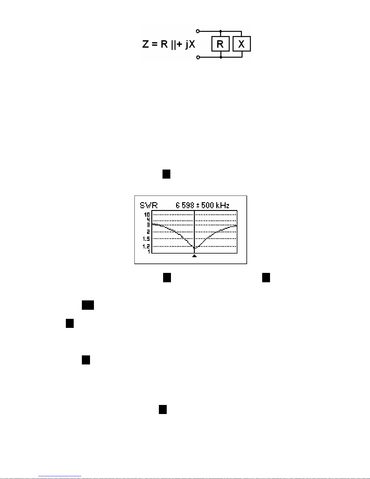
• In the parallel model, impedance is expressed as resistance and reactance
connected in parallel:
9
4.3. Graph modes
A key feature of RigExpert AA-200/AA-500 Antenna Analyzers is ability to display
various parameters of a load graphically. Graphs are especially useful to view the
behavior of these parameters over the specified frequency band.
4.3.1. SWR graph
In the SWR graph mode (press the 4 key in the Main menu), values of the Standing
Wave Ratio are plotted over the specified range:
You may set center frequency (the 2 key) or scanning range (the 3 key). By using
arrow keys, these parameters may be increased or decreased.
Press the ok key to refresh the graph.
The 0 key opens a list of radio amateur bands to set the required center frequency and
scanning range quickly. Also, you may use this function to see the whole frequency
range supported by the analyzer.
Press the 1 key to access the list of additional commands for this mode.
4.3.2. R,X graph
In the R,X graph mode (press the 5 key in the Main menu), values or R (active part of
the impedance) and X (reactive part) are plotted as solid and dotted lines, respectively.

10
R,X graph - series model R||,X|| graph - parallel model
In these graphs, positive values of reactance (X) correspond to inductive load, while
negative values correspond to capacitive load. Please notice the difference in the plots
when series or parallel model of impedance is selected through the Settings menu.
[Please notice that RigExpert AA-500 displays absolute value of the reactance, |X|.]
4.3.3. Memory operation
In the SWR graph and R,X graph modes, you may choose to scan to memory (the 6
key). There are 100 memory slots available. Later, you may recall ( 9 ) the plots from
the specified memory.
Additionally, the F + 9 combination opens the editor of memory slot names.
4.4. Settings menu
The Settings menu (press the 0 key in the Main menu) contains various settings for the
analyzer.
When setting a longer LCD backlit timer, please notice that the backlit discharges the
accumulator heavily. It is recommended to keep the backlit turned off, when possible.
4.5. Computer connection
RigExpert AA-200/AA-500 Antenna Analyzers may be connected to the personal
computer for displaying measurement results on its screen, taking screen shots of the
LCD, as well as for updating the firmware.
A conventional USB cable may be used for this purpose. The supporting software is
located on the supplied CD.

11
4.6. Charging the accumulator
Use the supplied DC adapter or any other 9…14V DC source as an external charger for
the built-in Ni-MH accumulator. A car lighter cable may be used for this purpose.
You may have the charger connected while operating the analyzer. However, this will
take almost no effect if the LCD backlit is turned on and/or one of the continuous
measurement modes is active.
If the analyzer is being used for the first time, perform a full 10…12-hour charging
cycle.
When the accumulator is full, it starts heating (instead of absorbing electric energy). It
is a good idea to stop charging if the accumulator becomes warm. While it is safe to
leave the charging mode for a long period of time, it is recommended to do this no
more than 10…12 hours.

12
5. Applications
5.1. Antennas
5.1.1. Checking the antenna
It is a good idea to check an antenna before connecting it to the receiving or
transmitting equipment. The SWR graph mode is right for this purpose:
The above picture shows SWR graph of the vertical VHF antenna connected via the 40
m (131 ft) cable. The operating frequency is 146.2 MHz. The SWR at this frequency is
about 1.1, which is acceptable.
The next screen shot shows SWR graph of the simple dipole antenna with desired
operating frequency of 14.1 MHz:
The actual resonant frequency is about 13.4 MHz, which if too far from the desired
one. The SWR at 14.1 MHz is about 2.5, which is not acceptable in most cases.
5.1.2. Adjusting the antenna
When the measurement diagnoses that the antenna is off the desired frequency, the
analyzer can help in adjusting it.

13
Physical dimensions of a simple antenna (such as a dipole) can be adjusted knowing
the actual resonant frequency and the desired one.
Other types of antennas contain more than one element to adjust (including coils,
filters, etc.), so this method will not work. Instead, you may use the SWR mode or the
Show all mode to continuously see the result while adjusting various parameters of the
antenna.
For multi-band antennas, use the Multi SWR mode. You may easily see how one of the
adjustment elements (trimming capacitor, coil, physical length of an aerial) affects
SWR at up to five different frequencies.
5.2. Coaxial lines
5.2.1. Open- and short-circuited cables
Open-circuited cable Short-circuited cable
The above pictures show R and X graphs for a piece of cable with open- and shortcircuited end. A resonant frequency is a point at which X (see the dotted line) equals to
zero:
• In the open-circuited case, resonant frequencies correspond to (left to right) 1/4,
3/4, 5/4, etc. of the wavelength in this cable;
• For the short-circuited cable, these points are located at 1/2, 1, 3/2, etc. of the
wavelength.
[Please notice that RigExpert AA-500 displays absolute value of the reactance, |X|.]
5.2.2. Cable length measurement
Resonant frequencies of a cable depend on its length as well as on the velocity factor.
A velocity factor is a parameter which characterizes the slowdown of the speed of the
wave in the cable compared to vacuum. The speed of wave (or light) in vacuum is
known as the electromagnetic constant: c=299792458 meters per second or 983571056
feet per second.

14
Each type of cable has different velocity factor: for instance, for RG-58 it is 0.66.
Notice that this parameter may vary depending on the manufacturing process and
materials the cable is made of.
To measure the physical length of a cable,
1. Locate a resonant frequency by using single-point measurement mode or R,X
graph.
Example:
The 1/4-wave resonant frequency of
the piece of open-circuited RG-58 cable
is 4835 kHz
[Please notice that RigExpert AA-500 displays absolute value of the reactance.]
2. Knowing the electromagnetic constant and the velocity factor of the particular
type of cable, find the speed of electromagnetic wave in this cable.
Example:
299792458 * 0.66 = 197863022 meters per second
- or 983571056 * 0.66 = 649156897 feet per second
3. Calculate the physical length of the cable by dividing the above speed by the
resonant frequency (in Hz) and multiplying the result by the number which
corresponds to the location of this resonant frequency (1/4, 1/2, 3/4, 1, 5/4, etc.)
Example:
197863022 / 4835000 * (1/4) = 10.23 meters
- or 649156897 / 4835000 * (1/4) = 33.56 feet
(The actual length of this cable is 10.09 meters of 33.1 feet, which is
about 1% off the calculated result.)

15
5.2.3. Velocity factor measurement
For a known resonant frequency and physical length of a cable, the actual value of the
velocity factor can be easily measured:
1. Locate a resonant frequency as described above.
Example:
10.09 meters (33.10 feet) of open-circuited cable.
Resonant frequency is 4835 kHz at the 1/4-wave point.
2. Calculate the speed of electromagnetic wave in this cable. Divide the length by
1/4, 1/2, 3/4, etc. (depending on the location of the resonant frequency), then
multiply by this frequency (in Hz).
Example:
10.09 / (1/4) * 4835000 = 195140600 meters per second
- or -
33.10 / (1/4) * 4835000 = 640154000 feet per second
3. Finally, find the velocity factor. Just divide the above speed by the
electromagnetic constant.
Example:
195140600 / 299792458 = 0.65
- or 640154000 / 983571056 = 0.65
5.2.4. Cable fault location
To locate the position of the probable fault in the cable, just use the same method as
when measuring its length. Watch the behavior of the reactive component (X) near the
zero frequency:
• If the value of X is moving from -∞ to 0, the cable is open-circuited.
• If the value of X is moving from 0 to +∞, the cable is short-circuited.
[Please notice that RigExpert AA-500 displays absolute value of the reactance.]

16
5.2.5 Making 1/4-λ, 1/2-λ and other coaxial stubs
Pieces of cable of certain electrical length are often used as components of baluns
(balancing units), transmission line transformers or delay lines.
To make a stub of the predetermined electrical length,
1. Calculate the physical length. Divide the electromagnetic constant by the
required frequency (in Hz). Multiply the result by the velocity factor of the
cable, then multiply by the desired ratio (in respect to λ).
Example:
1/4- λ stub for 28.2 MHz, cable is RG-58 (velocity factor is 0.66)
299792458 / 28200000 * 0.66 * (1/4) = 1.75 meters
- or 983571056 / 28200000 * 0.66 * (1/4) = 5.75 feet
2. Cut a piece of cable slightly longer than this value. Connect it to the analyzer.
The cable must be open-circuited at the far end for 1/4-λ, 3/4-λ, etc. stubs, and
short-circuited for 1/2-λ, λ, 3/2-λ, etc. ones.
Example:
A piece of 1.85 m (6.07 ft) was cut. The margin is 10 cm (0.33 ft). The
cable is open-circuited at the far end.
3. Switch the analyzer to the Show all measurement mode. Set the frequency the
stub is designed for.
Example:
28200 kHz was set.
4. Cut little pieces (1/10 to 1/5 of the margin) from the far end of the cable until the
X value falls to zero (or changes its sign). Do not forget to restore the opencircuit, if needed.
Example:
11 cm (0.36 ft) were cut off.

17
5.2.6. Measuring the characteristic impedance
The characteristic impedance is one of the main parameters of any coaxial cable.
Usually, it is printed on the cable by the manufacturer. However, in certain cases the
exact value of the characteristic impedance is unknown or is in question.
To measure the characteristic impedance of a cable,
1. Connect a non-inductive resistor to the end of the cable. The value of this
resistor is not important. However, it is recommended to use 50 to 100 Ohm
resistors.
Example 1: RG-58 cable with 51 Ohm resistor at the far end.
Example 2: Unknown cable with 51 Ohm resistor at the far end.
2. Enter the R,X graph mode and make measurement in the full frequency range.
Example 1: RG-58 cable
Example 2: Unknown cable
[Please notice that RigExpert AA-500 displays absolute value of the reactance.]
3. Changing the display range and performing additional scans, find a frequency
where R (solid line) reaches its maximum, and another frequency with
minimum. At these points, X (dotted line) will cross the zero line.
Example 1: 6.5 MHz - max., 12.25 MHz - min.
Example 2: 13.25 MHz - max., 29.5 MHz - min.

18
4. Switch the analyzer to the Show all measurement mode and find values of R at
the previously found frequencies.
Example 1: 54.4 Ohm - max., 51.1 Ohm - min.
Example 2: 75.2 Ohm - max, 52.1 Ohm - min.
5. Calculate the square root of the product of these two values.
Example 1: sqrt (54.4 * 51.1) = 52.7 Ohm
Example 2: sqrt (75.2 * 52.1) = 62.6 Ohm
5.3. Measurement of other elements
Although the analyzer is designed for use with antennas and antenna-feeder paths, it
may be successfully used to measure parameters of other RF elements.
5.3.1. Capacitors and inductors
RigExpert AA-200/AA-500 Antenna analyzers can measure capacitance from a few pF
to about 1 µF as well as inductance from a few nH to about 100 µH.
Be sure to place the capacitor or the inductor as close as possible to the RF connector
of the analyzer.
1. Enter the R,X graph mode and select the full scanning range. Perform a scan.
Example 1: Example 2:
Unknown capacitor Unknown inductor
2. By using left and right arrow keys, scroll to the frequency where X is -25…-100
Ohm for capacitors or 25…100 Ohm for inductors. Change the scanning range
and perform additional scans, if needed.
[Please notice that RigExpert AA-500 displays absolute value of the reactance.]
3. Switch to the Show all mode and read the values of capacitance or inductance.

19
Example 1: Example 2:
Unknown capacitor Unknown inductor
[Since RigExpert AA-500 can not determine the sign of reactance, it displays both L
and C parameters.]
5.3.2. Transformers
The analyzer can be used for checking RF transformers. Connect a 50 Ohm resistor to
the secondary coil (for 1:1 transformers) and use SWR graph or R,X graph modes to
check the frequency response of the transformer. Similarly, use resistors with other
values for non-1:1 transformers.
5.4. RF signal generator
The output signal level is about +10 dBm for RigExpert AA-200 and about +5 dBm for
RigExpert AA-500 (at the 50 Ohm load). Therefore these analyzers can be used as a
source of RF signal for various purposes. Enter the SWR mode or the Show all mode,
press ok to start, then press the 2 key to generate the uninterrupted RF signal.

20
Copyright © 2007-2008 Rig Expert Ukraine Ltd.
http://www.rigexpert.com
RigExpert is a registered trademark of Rig Expert Ukraine Ltd.
 Loading...