

Page 1
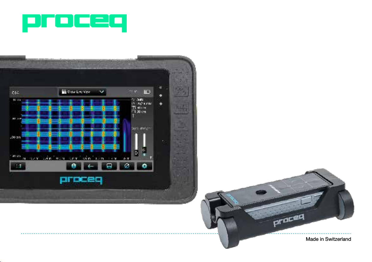
PROFOMETER® PM-6
OPERATING INSTRUCTIONS
60 Years of Innovation
60 Years of Innovation
Made in Switzerland
Made in Switzerland
Page 2

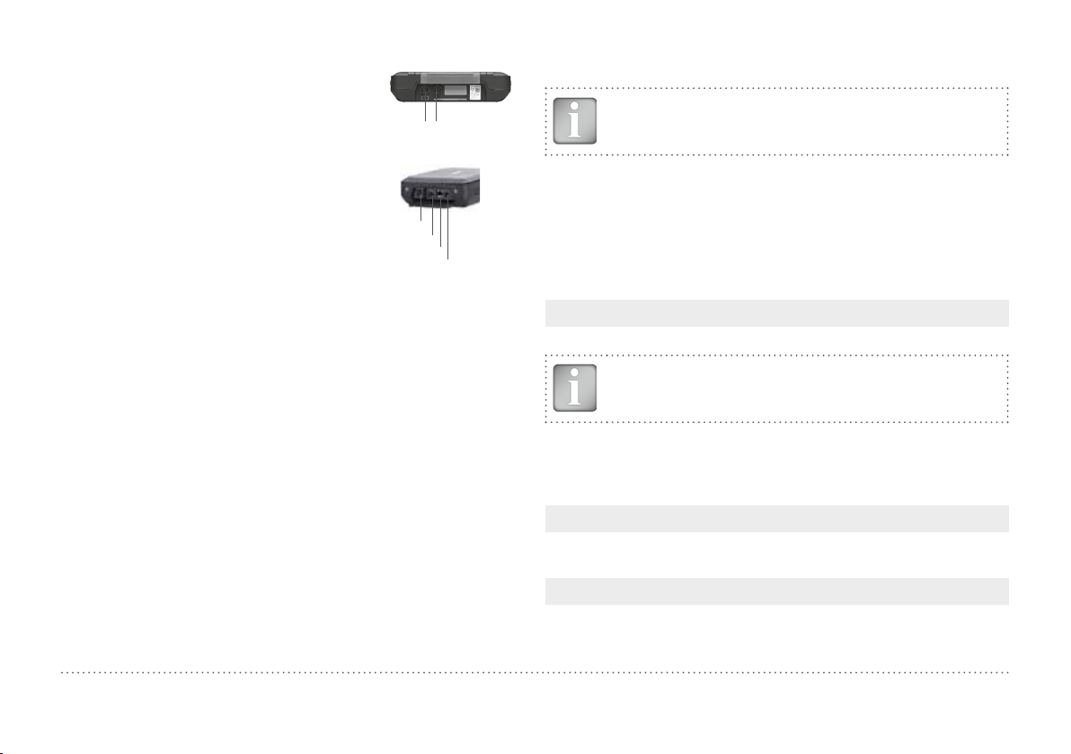
Scope of Delivery
A
C D
A
Profometer Touchscreen Unit
B
Battery complete
B
E
C
Universal Probe with Cart
D
Profometer PM-6 probe
Cable 1.5 m
E
Power Supply with cable
(USA, UK or EU)
F
USB Cable 1.8 m (6 ft)
G
DVD with Software
H
Documentation
I
Carrying Strap complete
F
G
© 2014 Proceq SA 2
H
I
Page 3

Overview
5
12
4
12
1
1
11
10
11
1212
3 © 2014 Proceq SA
9
12
2
11
12
8
12
3
11
7
6
12
Press to power on. To power off
press again and tap “X Off” on
the screen.
Soft Key – Switches in and out
of full screen view.
Back Button – Returns to
previous screen.
Page 4
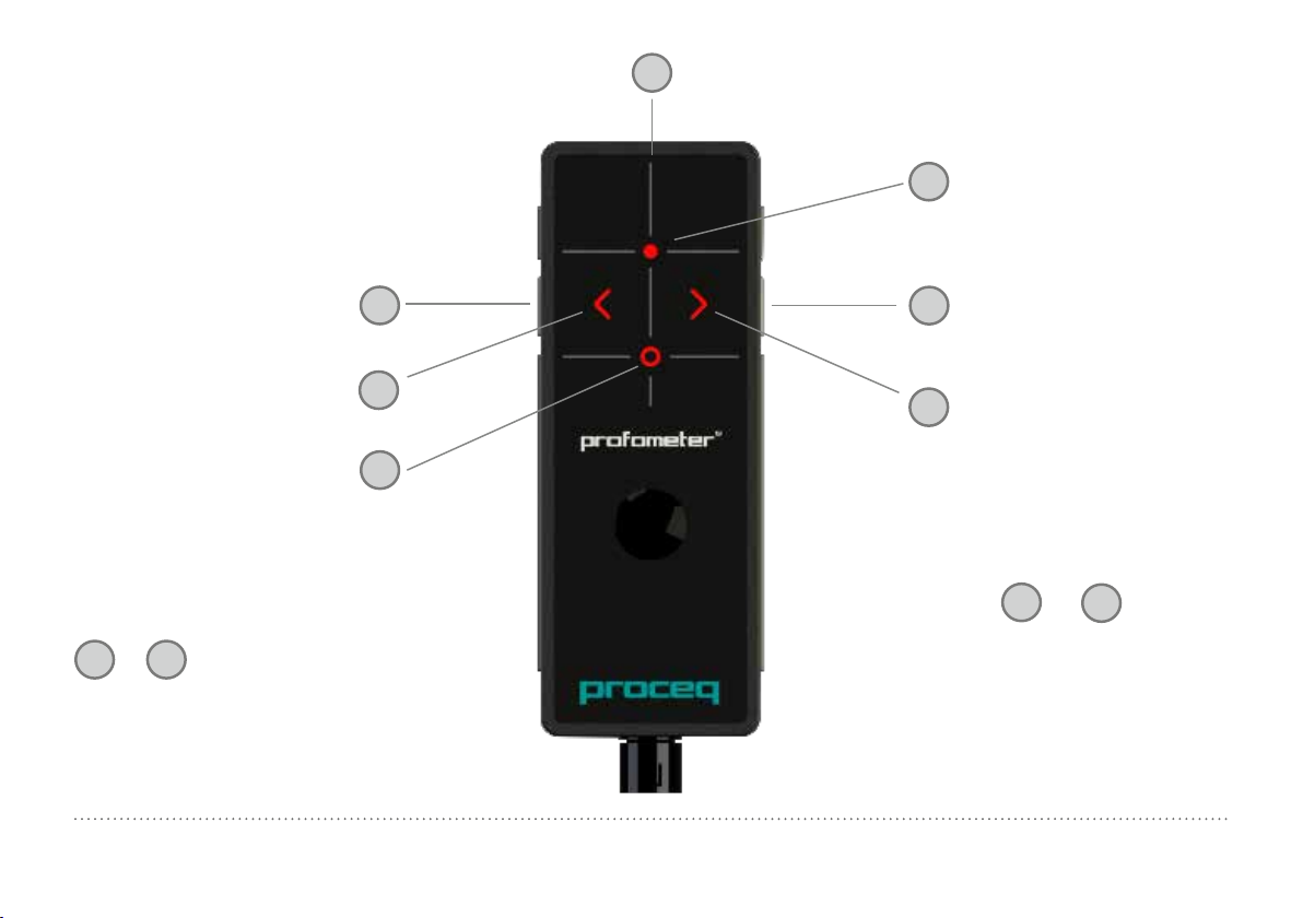
Center Line (CL)
16
Measurement Center when
15
Spot range is set (MC Sp)
Short: Start / Stop
Long: Set marker
Arrow LED indicates proximity of rebar*
Measurement Center when Standard,
Large or Auto range is set (MC SLA)
*When an Arrow LED lights up move the
probe along the rebar axis until MC LED
or 15 lights up. Then the MC is
14
precisely above a rebar axis.
© 2014 Proceq SA 4
12
17
14
Short: Measure diameter
13
Long: Zeroing
Arrow LED indicates proximity of rebar*
17
By pushing
ously the cursor jumps to the next line
(in Multi-Line, Area-Scan and Cross-Line
Mode only)
12
and 13 simultane-
Page 5

Table of Contents
1. Safety and Liability ...................................................6
1.1 General Information ...........................................................6
1.2 Liability ...............................................................................6
1.3 Safety Instructions ............................................................6
1.4 Correct Usage ...................................................................6
2. Measuring Principle ..................................................... 7
2.1 Measuring Principle ..........................................................7
2.2 Calibrated Measuring with Profometer PM-6 ..................7
2.3 The
2.4 Resolution ..........................................................................8
2.5 Sphere of influence by Ferromagnetic Material ...............8
Measuring
Range................................................ 7
3. Operation ...................................................................... 8
3.1 Getting Started ..................................................................8
3.2 Main Menu .........................................................................9
3.3 Settings ..............................................................................9
3.4 Measurement Screen ......................................................11
3.5 Measurement Modes and Storage of Data ....................12
3.6 Review of Data ................................................................18
3.7 Practical Hints .................................................................24
4. Explorer Document Handling ..................................... 27
5. Ordering Information ................................................. 28
5.1 Units .................................................................................28
5.2 Upgrades .........................................................................28
5.3 Parts and Accessories ....................................................28
6. Technical Specifications ............................................ 29
7. Maintenance and Support ......................................... 30
7.1 Maintenance and Cleaning .............................................30
7.2 Support Concept .............................................................30
7.3 Standard Warranty and Extended Warranty ..................30
7.4 Disposal ...........................................................................30
8. PM-Link Software ...................................................... 30
8.1 Starting PM-Link .............................................................30
8.2 Adjusting Settings ...........................................................32
8.3 Exporting Data .................................................................33
8.4 Deleting Data ...................................................................35
8.5 Further Functions ............................................................35
9. Appendices ................................................................. 35
9.1 Appendix A1: Rebar Diameters ......................................35
9.2 Appendix A2: Neighboring Bar Correction .....................36
9.3 Appendix A3: Minimum / Maximum Cover ....................36
© 2014 Proceq SA 5
Page 6

1. Safety and Liability
1.1 General Information
This manual contains important information on the safety, use and maintenance of the Profometer PM-6. Read through the manual carefully before the first use of the instrument. Keep the manual in a safe place for
future reference.
1.2 Liability
Our “General Terms and Conditions of Sales and Delivery” apply in all
cases. Warranty and liability claims arising from personal injury and damage to property cannot be upheld if they are due to one or more of the
following causes:
• Failure to use the instrument in accordance with its designated use as
described in this manual.
• Incorrect performance check for operation and maintenance of the instrument and its components.
• Failure to adhere to the sections of the manual dealing with the performance check, operation and maintenance of the instrument and its
components.
• Unauthorised modifications to the instrument and its components.
• Serious damage resulting from the effects of foreign bodies, accidents,
vandalism and force majeure
All information contained in this documentation is presented in good faith
and believed to be correct. Proceq SA makes no warranties and excludes
all liability as to the completeness and/or accuracy of the information.
1.3 Safety Instructions
The equipment is not allowed to be operated by children or anyone under
the influence of alcohol, drugs or pharmaceutical preparations. Anyone
who is not familiar with this manual must be supervised when using the
equipment.
• Carry out the stipulated maintenance properly and at the correct time.
• Following completion of the maintenance tasks, perform a functional
check.
1.4 Correct Usage
• The instrument is only to be used for its designated purpose as describe herein.
• Replace faulty components only with original replacement parts from
Proceq.
• Accessories should only be installed or connected to the instrument
if they are expressly authorized by Proceq. If other accessories are
installed or connected to the instrument then Proceq will accept no
liability and the product guarantee is forfeit.
6 © 2014 Proceq SA
Page 7
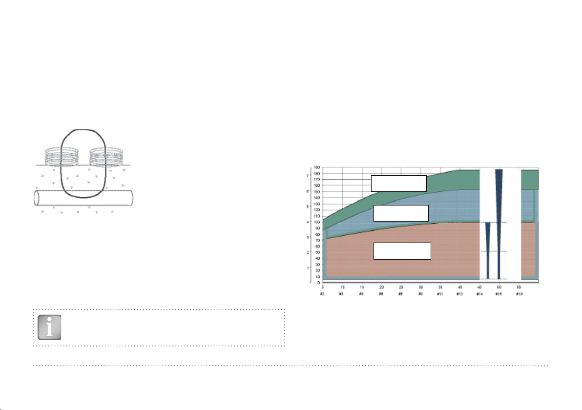
2. Measuring Principle
2.1 Measuring Principle
The Profometer PM-6 uses electromagnetic pulse induction technology
to detect rebars. Coils in the probe are periodically charged by current
pulses and thus generate a magnetic field. On the surface of any electrically conductive material which is in the magnetic field, eddy currents are
produced. They induce a magnetic field in the opposite direction. The
resulting change in voltage can be utilized for the measurement.
Coils
Magnetic Field
Concrete
Rebar
Figure 1: Measurement principle
The Profometer PM-6 uses different coil arrangements to generate several magnetic fields. Advanced signal processing allows locating a rebar
as well as measuring of cover and rebar diameter.
This method is unaffected by all non conductive materials such as concrete, wood, plastics, bricks etc. However any kind of conductive materials within the magnetic field (sphere of approx. 200 mm / 8 inch radius)
will have an influence on the measurement.
NOTE! Remove all metallic objects such as rings and watches before you start measuring.
2.2 Calibrated Measuring with Profometer PM-6
The Profometer PM-6 is calibrated to measure on a normal rebar arrangement; which is an arrangement of non-stainless steel rebars fastened with binding wires only e. g. when measuring on welded mesh
wires the cover and diameter readings must be corrected (see “3.7 Practical Hints”). The following information on accuracy, measuring ranges
and resolutions refer to measurements on normal rebar arrangements.
2.3 The
The measuring range is dependent on the bar size. The expected accuracy of the cover measurement is indicated in the graphic below. It
complies with BS1881 part 204, for a single rebar with sufficient spacing.
[inch] [mm]
Cover depth
Up to the indicated limits the cover is measured and displayed.
In the Locating Mode a rebar is shown. In the Single-Line Mode the cover curve is shown but a
rebar is only set up to 90 % of the maximum cover.
Figure 2: Measuring ranges and accuracy
Measuring
Range
Large
measuring range
Spot probe
measuring range
Standard
measuring range
Rebar size
185 mm
153 mm
100 mm
50 mm
±3 mm
measuring
±2 mm
±1 mm
±1 mm
accuray
[mm]
1
/16 inch]
[
© 2014 Proceq SA 7
Page 8
2.4 Resolution
There is a limit to the minimum spacing of bars
depth and rebar diameter. It is impossible to distinguish between individual bars above these
C
[inch]
[mm]
C
Spot probe
range
Cover depth
Standard
range
S
limits.
Large range
Below the curve:
Individual rebar can be detected
Rebar spacing
Figure 3: Resolution
depend
Ø 40 mm
Ø 26 mm
Ø 16 mm
Ø 12 mm
Ø 8 mm
[mm]
S
[inch]
ing on the cover
# 13
# 12
# 8
# 5
# 4
# 3
# 2
2.5 Sphere of influence by Ferromagnetic Material
Sphere of influence: Diameter 400 mm / 16 inch
NOTE! This effect can be reduced by the neighboring bar
corretion implemented in the Profometer PM-6.
3. Operation
3.1 Getting Started
Battery Installation
To install the Battery (B) into the Profometer Touchscreen Unit (A), lift the
stand as shown. Insert the battery and fasten in place with the screw.
Figure 5: Insert Battery
There are two status LEDs
LED is red while charging and turns to green when it is fully charged. The
other LED is application specific.
NOTE! Only use the power supply provided.
and above them a light sensor. The upper
1
Any ferromagnetic material within the
sphere may have an influence on the
signal value (e. g. during a reset)
• A complete charge requires <9h (Instrument not operating)
• Charging time is much longer if the instrument is in use.
• An optional quick charger (Part No. 327 01 053) can be used to charge
MC (SLA)
14
a spare battery or to charge the battery outside of the instrument. In
this case it takes <5.5 h for a complete charge.
Figure 4: Influence sphere
8 © 2014 Proceq SA
Page 9
Connect the Universal Probe (C) to one of the
sockets on the upper side of Profometer Touchscreen Unit (A) using the Probe Cable (D).
Probe Connections
3.3 Settings
NOTE! The settings must be checked prior to each measurement.
USB Host:
Connect a mouse, keyboard or USB stick.
USB Device:
Connect application specific probes and PC.
Ethernet:
Connection for firmware upgrades.
USB Host
USB Device
Ethernet
Power Supply
Power Supply:
Connect the power supply through this
connection.
Figure 6: Top and left
views
3.2 Main Menu
On start up the main menu is displayed. All functions may be accessed
directly via the Touchscreen. Return to the previous menu by pressing the
back button or the return icon (arrow) at the top left of the Touchscreen.
Measurement: Application specific measurement screen.
Settings: For application specific settings.
Explorer: File manager functionality for reviewing measurements
saved on the instrument.
System: For system settings, e. g. language, display options.
Information: For device information and remaining storage capacity.
Off: Power off.
Scroll up and down the screen by dragging your finger up or down the
screen. The current setting is displayed on the right hand side. Tap on an
item to adjust it.
1)
For the scanning in Y-direction in the Cross-Line Mode the diameter, respectively spacing for rebars running in X-direction can be set in addition.
2)
Settings can be changed in files already stored.
Measuring Range
Select between Standard, Large or Auto ranges (see Figure 2).
NOTE! The range cannot be changed during the measurement. To change the range, store the data first and open a
new file.
Standard is the default setting, because it is the most accurate one.
Auto switches automatically between Standard and Large. Spot should
be selected for measurements on small areas, in corners and on rebar
arrangements with small spacing.
Rebar Diameter Scan-X / Rebar Diameter Scan-Y
Select the Rebar Diameter (6 to 40 mm / #2 to #12, see Appendix A1),
either determined from the drawing or as measured.
Neighboring Rebar Correction Spacing for Scan-X / Scan-Y
It mitigates the influence of neighboring rebars. By setting the spacing
to the rebars running parallel to the rebar on which the measurement
1) 2)
1) 2)
© 2014 Proceq SA 9
Page 10
is taking place, the diameter and the cover are automatically corrected.
This is possible for rebar spacing from 50 to 130 mm / 2.00 to 5.20 inch
(see Appendix A2).
2)
Unit
Select Metric, Metric Japanese, Imperial or Imperial Diameter, Metric
Cover and Distance.
Minimum Cover
2)
A Minimum Cover value from 10 to 142 mm / 0.40 to 5.56 inch can be
set in 1 mm / 0.04 inch steps (see Appendix 3). In the Single-Line, MultiLine and Cross-Line Mode/View rebars with less cover than minimum
cover will be shown in red color. In the Single-Line View and Statistical
View a horizontal, respectively vertical dotted line in red indicates the
Minimum Cover value set.
Cover Offset
2)
When a Cover Offset value is set the measured cover will be reduced by
this value; e. g. when a wooden or plastic plate is used to measure with
the probe cart on rough surfaces (see “3.7 Practical Hints”). In this case
the plate thickness must be set as Cover Offset value). A value from 1 to
50 mm / 0.04 to 1.92 inch can be set.
Display Inclined Rebar
By setting this feature the inclined rebar is displayed in the Locating Mode
when all four wheels of the cart have passed over the inclined rebar. In
the Single-Line and Multi-Line Modes it is only shown in the cart symbol.
NOTE! In areas with small rebar spacing this feature may not
work properly.
NOTE! To get smooth color intervals the Minimum and Maximum Cover should be set in 5 mm / 0.20 inch steps.
Sharpen
2)
With this setting the signal strength color spectrum of the Multi-Line and
Maximum Cover
2)
A Maximum Cover value from 20 to 190 mm / 0.80 to 7.48 inch can be
set in steps of 1 mm / 0.04 inch (see Appendix A3). In the Single-Line,
Multi-Line and Cross-Line Mode/View rebars with cover more than Maximum Cover will be shown in grey color.
NOTE! The Maximum Cover must be at least 10 mm / 0.40
inch higher than the Minimum Cover. If not, the instrument
will correct it automatically.
The Maximum Cover should also be set for different files measured on
the same surface to get the same color range for comparison purpose.
Cross-Line Views can be sharpened.
Display Curve
2)
Select Cover Value, Signal Strength or None. The respective curve or
no curve is displayed in Single-Line View.
Align Rebar Positions
2)
When measuring in the Multi-Line or Cross-Line Mode along at least two
lines of at least 55 cm / 22.00 inch length, the rebar positions of the last
line are aligned to the rebar positions of the two previous lines.
NOTE! This feature should only be set, if the rebars are running
parallel to the Start line (X- or Y-line). It is not activated during
the measurements (activated only when storing the data).
10 © 2014 Proceq SA
Page 11
Return to start on new line
3
With this feature set, the cursor jumps back to the start line when changing line in the Multi-Line and Cross-Line Modes.
Line Height (in Y-direction)
The line height must be set in the Multi-Line, Area-Scan and Cross-Line
Modes. It determines the spacing between the measuring rows. A height
5 to 203 cm / 2.00 to 80.00 inch can be set.
Grid Width (in X-direction)
The grid width must be set in the Area-Scan and Cross-Line Modes. A
width from 5 to 203 cm / 2.00 to 80.00 inch can be set.
3.4 Measurement Screen
The standard measurement screen is shown on page 3. All settings are
directly accessible from the measurement screen.
Zoom in by placing thumb and index finger together on the
screen and spreading them apart. This can be used in both the
horizontal and vertical directions when making a measurement.
Zoom out by placing thumb and index finger apart on the
screen and pinching them together.
Pan the image from left to right by dragging.
Measuring screen controls (see page 3)
File name: Enter the file name and tap return. Saved measure-
1
ments will be stored with this file name. If several measurements
are made under the same filename, a suffix increments after each
measurement and follows the file name.
Measurement Mode: Select the type of measurement to be carried
2
3
out (see “3.5 Measurement Modes and Storage of Data”).
The top right hand corner of the display shows the current time, the
3
3
battery status and a warning triangle for zeroing the probe: after 5
minutes in orange, after 10 minutes in red.
NOTE! Tap on the triangle to perform zeroing.
Display of selected Settings and Screen Mode:
4
3
3
3
3
3
3
3
3
5
6
7
8
9
10
11
– Measuring Range
– Rebar Diameter
– Neighboring Rebar Correction
– Cover Offset
– Lin e Heigh t (for Multi-Line, Area-Scan & Cross-Line Mode only)
– Grid Width (for Area-Scan and Cross-Line Mode only)
– Probe Direction X: Undefined direction
^, v, <, >: On vertical wall, probe head
towards up, down, left, right
_, ˉ: On horizontal surface, on soffit
Settings: Switches to the settings menu (see “3.3 Settings”).
Rebar Diameter: Measuring or change setting of rebar diameter
Start:
Restart with measurements and reposition cursor to the start line.
(All data of current measurements are deleted)
File Info or delete, Cursor to Start line in Multi-Line and Area-Scan
Modes
Zoom in to cursor position (for Single-Line Mode only)
Set cursor to line below or above (for Multi-Line Mode only)
Zoom to fit During measurement: Goes back to standard view
Stored file: Complete measuring area is displayed.
In the Modes/Views “Zoom to fit” does not show all the details
for scanning distance > 10/30 meters (> 32.8/98.4 feet).
Measurements or store measured data
© 2014 Proceq SA 11
Page 12
3.5 Measurement Modes and Storage of Data
When Measurement Mode is selected for the first time after switching
on the instrument, zeroing of the probe is performed. Confirm it and wait
for the button assessment window. Wait or tap anywhere on the screen.
The Measurement Modes available are shown at
screen.
Locating Single-Line Multi-Line Area-Scan Cross-Line
PM-600
PM-630
PM-650
•
• • • •
• • • • •
NOTE! Valid for all Measuring Modes: In case measuring data
shall be stored create a folder in the Explorer (see “4. Explorer
Document Handling”) and check if the correct folder is active.
Stored files can be reopened to continue with the measurements.
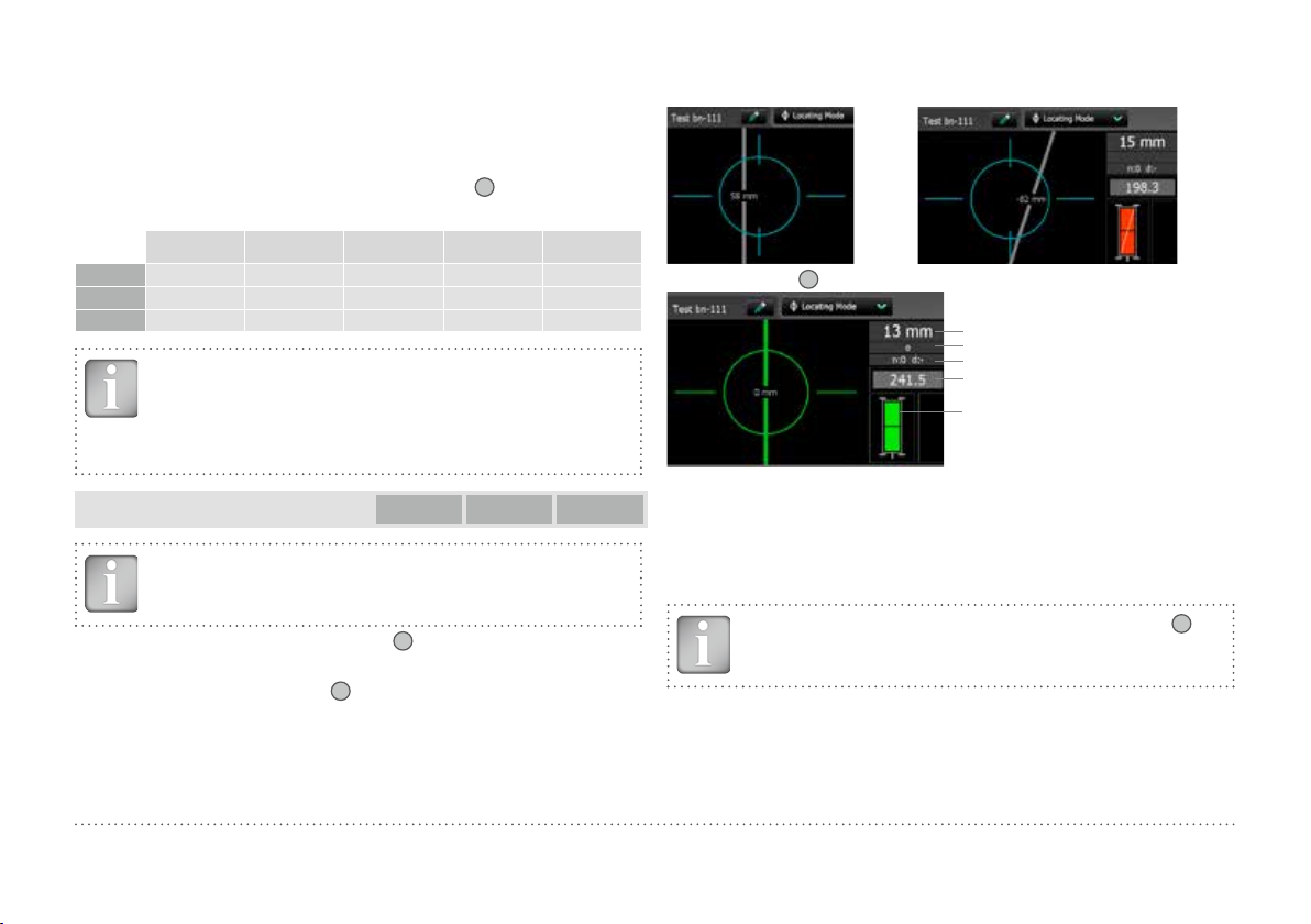
Locating Mode
PM-600 PM-630 PM-650
NOTE! The Locating Mode is the default mode because all
measurements should start with this mode.
2
on the measuring
Approaching a rebar Rebar is inclined to the CL
When the Center Line
is precisely over the rebar (red LED of probe center is lit) it shows:
16
(minimum inclination for a display is 6 degrees).
Actual Cover
Distance to next rebar
Nos./Meas. diameter
Signal strength
Both rectangles Green:
Ideal probe position:
Both coils maximum signal strength and
green
Bad probe position:
Coil rectangles of different size and red
A rebar is shown only within the cover
ranges indicated in Figure 2.
Figure 7: Screens of Locating Mode
• Enter the setting menu by tapping on
5
. Set the correct settings, es-
pecially Measuring Range and Display Inclined Rebar (on or off)
• Hold the probe cart with the CL
16
parallel to the assumed direction of the
rebar to be scanned. Then scan perpendicular to the CL until the probe
cart crosses a rebar. The display shows (only if probe is fixed on the cart):
NOTE! The prope position indication refers always to
(SLA), even the Spot Range is set.
In most cases the rebars of the first and second layers are fixed in a rectangular mesh (e. g. vertical and horizontal rebars in a wall).
14
MC
12 © 2014 Proceq SA
Page 13

In case an inclined rebar is displayed,
one has to find out the exact rebar direction.
14
15
MC
• For this purpose locate the rebar as
/
described below, but first remove the
probe from the cart.
14
• Once the MC
15
/
is above the re-
Center point
bar axis mark the position of the MC
on the surface at CL
edge of the probe and on either side
of the MC.
16
at the upper
Direction of rebar
L
• Position the CL point at the lower
edge of the probe precisely at the
marked center point.
• Turn the probe around this center
point until the maximum signal is
displayed. (Placing a set square with
one corner at the center point facilitates the turning of the probe).
The CL
16
runs parallel to and above
the rebar axis, when the signal strength
reaches the maximum and the MC
15
lights up.
14
/
Figure 8: Finding the rebar
direction
Center point
above rebar
Set square
R
Whenever possible start with locating the rebars of the first layer, e. g. on
a column the horizontal stirrups.
16
• Holding the CL
horizontally, move vertically up or down until the
the probe cart vertically until both rectangles in the probe symbol are
green and of equal, minimum size.
• Now move the probe cart horizontally until one of the Arrow LEDs
14
lights up and then move back until MC LED
or
15
lights up.
• At this position you may also measure the diameter either by pushing
13
on the right side of the probe or 6 on the Touchscreen (e. g. when
the probe is fixed to the telescopic extension rod).
• If the spacing of parallel rebars is between 5 and 13 cm (2.00 to 5.20
inch), set the respective Neighboring Rebar Correction value first.
If the cover is too small for diameter measurement “too close” is displayed.
• In this case place a wooden or plastic board on the surface and set the
board thickness as Cover Offset to measure the diameter.
Finally the measured diameter must be set. The cover reading will be corrected according to the diameter set.
NOTE! For more details about diameter measurement see
“3.7 Practical Hints”.
7
• Tap
to store the diameter and cover measurement.
• Repeat this procedure at each rebar.
The saved data can be seen in the Snapshot and Normal Statistics View
(see “3.6 Review of Data”).
NOTE! Cover values are only saved for later viewing, if the
diameter was measured and saved.
Arrow LED lights up and then move back until the MC LED lights up.
After having located the first layer rebars continue with locating the second layer rebars.
14
• Position the MC
15
/
at the mid line of the first layer rebars, e. g.
on a column hold the probe with the CL running vertically and move
© 2014 Proceq SA 13
17
Page 14

Single-Line Mode
PM-630 PM-650
NOTE! It is advisable to locate the first and second layer rebars with the Locating Mode to find the optimum line position prior to measuring with the Single-Line Mode.
The Single-Line Mode is mainly used if cover must be shown along one
line on a rather long distance (e. g. in a tunnel). Therefore the measurements are made across the first layer rebars.
The maximum scan length is 999 m / 3’280 feet in each direction (to the
right and to the left from the zero line).
• Enter the setting menu by tapping on
5
. Set the correct settings, es-
pecially Rebar Diameter, Unit, Minimum Cover and Display Curve.
In case Single-Line scanning is done over rebars of different diameters
and/or of different spacing measure each diameter.
• Position the probe cart at the start line in an optimum position (the MC
15
14
/
at the mid line of the rebars running parallel to the moving direc-
tion, both rectangles in the probe symbol are of equal minimum size).
• In case
is shown at 7 tap on it and will be shown.
• Start with the measurement if the cursor is at the start line. If not perform a reset
8
.
• Move the probe cart with constant speed crosswise over the rebars,
not exceeding the maximum speed (speed bar half filled in green).
• Above each rebar, when the red LED of MC
/
lights up, you may
14
15
measure the rebar diameter and on completion, it will be displayed
in blue. The measured diameter may be deleted within 5 seconds by
tapping on 6.
• In case the spacing between the rebars is in the range of 5 to 13 cm
(2.00 to 5.20 inch), set the respective Neighboring Rebar Correction
value first (see Figure 26).
The cursor position can be adapted in two ways to changed cart position:
• Tap on the cursor and wait until it becomes white and orange. Move
the cursor to the desired position (even left to the zero line is possible). Be aware: Scanning is not anymore possible between the new
cursor position and the zero-line. Already scanned rebars cannot be
removed by a new scanning but you may scan again on the left of
the first rebar or on the right of the last rebar. To delete the already
scanned rebars tap
• Tap on
and set the required displacement distance. In case you
and .
must jump due to an obstacle like a column, move the cart until the
right wheels touch the column, set the displacement distance (column
width + 107 mm / 4.20 inch for the cart width) and reposition the cart
with the left wheels touching the column. Tap on / .
At the end when stopped scanning a marker (dotted blue line) is set.
Probe position
To see the actual cursor position short tap on the cursor and the position is shown in white on
the X-axis.
The rebars are displayed to scale depending on the diameter
The cover curve is shown (if selected) within the cover ranges indicated in Figure 2 but a rebar
will only be shown up to 90 % of those limits.
The actual position is shown in a resolution of ± 3 mm / 0.12 inch.
Red indicates rebars with insufficient cover, others with sufficient
cover.
Red dotted is the minimum
required cover. Blue number
indicates measured diameter.
Either the Cover, Signal Strength
or None curve can be displayed
by tapping on
ing “Display Curve”.
and chang-
14 © 2014 Proceq SA
Page 15

To display a rebar as a
circle zoom the horizontal
and vertical axis to the
same scale.
The spacings of the rebars
are shown in blue.
The distances from the
start line to the first rebar
and from the end line to
the last rebar are shown in
white color. If the figures
are not shown, zoom in.
In the Single-Line Mode one can also change from cover curve to signal
strength curve or no curve (see also “3.6 Review of Data”).
The path length measurement accuracy depends on the test surface. The
accuracy of measurements done on a smooth concrete surface (concrete
poured in metallic shuttering) is shown in the specifications, see “6. Technical Specifications”. On rougher surfaces the measured length may be
reduced or checked at certain intervals by setting markings on the test
surface and comparing with marks set on the display (long push on
After storage (tap
7
), the data can be seen in the Statistics View, the
12
).
Single-Line View and also in the Snapshot View if at least one diameter
was measured (see “3.6 Review of Data”).
PM-630 PM-650
Spacing between rebars (in blue)
Figure 9: Screen of Single-Line Mode with cover curve
• To change a diameter tap on the rebar.
A window opens.
• Tap on the window and change diameter.
To erase set diameter to zero.
The new diameter is set and shown in orange.
The cover changes accordingly but the cover
curve remains except above the rebar axis.
Multi-Line Mode
NOTE! It is advisable to locate the first and second layer rebars with the Locating Mode to find the optimum line position prior to measuring in the Multi-Line Mode.
The Multi-Line Mode is often used if cover, rebar location and rebar diameters of mainly rectangular areas of different sizes must be shown (see
“3.6 Review of Data”), thus mainly for the first layer rebars.
In one measuring sequence a maximum of 62 lines can be scanned and
stored in one file.
5
• Enter the settings menu by tapping
.
• Set the correct settings as for the Single-Line Mode. Additionally set
the Line Height. If desired, set also “Align Rebar Position” and “Return
to start on new line”.
NOTE! “Align Rebar Position” should only be set, if all rebars
are running parallel to the start line (Y-axis).
Figure 10: Single-Line View zoomed, showing change of rebar diameter
New set diameter shown in orange
© 2014 Proceq SA 15
Page 16

NOTE! For larger areas it is advisable not to set “Return to
start on new line” and to measure the lines alternatively start
to end, back from end to start.
• Position the probe cart at the first start line in a optimum position (the
15
14
MC
/
at the mid line of the rebars running parallel to the moving
direction, both rectangles in the probe symbol are green and of equal,
minimum size) and tap on reset 8 followed by tapping on .
• Move the probe cart crosswise over the rebars. Above each rebar,
14
when the red LED of MC
15
/
lights up, you may measure the rebar
diameter and on completion, it will be displayed. If the spacing between the rebars is in the range of 5 to 13 cm (2.00 to 5.20 inch), set
the respective Neighboring Rebar Correction value first.
At the end of the first line a marker (dotted blue line) is set.
To proceed with the next line tap
10
or push
12
13
and
simultaneously on
the probe. The cursor jumps to the next measuring row, either to the start
line or remains at the end line, depending on whether “Return to start on
new line” is set or not.
Changing the cursor position works like in the Single-Line Mode. Additionally one can change to another line within the displayed area (which
also can be changed as described in ”3.4 Measurement Screen”). However, to delete the already scanned rebars of one line set the cursor to
the zero line and tap
. By tapping on and all measured
data of all lines would be deleted.
At the start of each line you may change the probe direction (e. g. when
measuring on a wall along the bottom line close to the slab).
• Tap on
.The arrow in the probe cart symbol changes from to .
For the next line you may change back to .
NOTE! By changing the setting “Line Height” during the
measurements the height of all lines including the ones already measured will change and hence, also the line positions. Change the line height only if it was previously wrongly
set.
At each rebar you may measure the rebar diameter. At the end, set one
common diameter, normally the smallest one (see “3.7 Practical Hints”).
Figure 11 shows the rebars in a plan view in different colors depending on
the measured cover. Red means the cover is smaller than the minimum
set.
Rebars with insufficient cover in red, others have sufficient cover
Actual cover
Distance from MC to rebar
no. of snapshots/no. of rebars
/ last measured diameter
A rebar will only be shown up to 90 % of
the cover ranges indicated in Figure 2.
Accurate probe
position if
rectangles green
and of same size
cover ranges,
< xx in red
if minimum
cover set
Alternatively
diameter ranges
Figure 11: Screen of Multi-Line Mode
Alternatively the diameter can be displayed in different colors by tapping
on the cover spectrum. Rebars of which the diameter was not measured
or set are shown in white. Diameters measured are shown in the respective color. Diameters set in the Single-Line View are shown additionally
with an orange cross bar in the middle of the rebar (see Figure 20).
16 © 2014 Proceq SA
Page 17

After storage (tap 7 ), the data can be seen in the Statistics View, the
Single-Line View, the Multi-Line View and also in the Snapshot View if at
least one diameter was measured (see “3.6 Review of Data”).
In the Multi-Line View the signal strength spectrum can be seen in addition to the cover and diameter, see “3.6 Review of Data”.
Area-Scan Mode
PM-630 PM-650
NOTE! It is advisable to locate the first and second layer rebars with the Locating Mode to find the optimum line position prior to measuring in the Area-Scan Mode.
The Area-Scan Mode is mainly used to show the first layer rebar covers
on large areas, e.g. of concrete slabs in car parks. The measuring procedure is the same as for the Single-Line, respectively Multi-Line Mode.
The Area-Scan Mode is best suited for a combination with potential field
measurements; e. g. combined with Canin+ measurements. But in this
case the line height and grid width must be the same for both measurements (square grid required by Canin ProVista).
5
• Enter the settings menu by tapping
.
• Set the correct settings as for the Single-Line and Multi-Line Mode.
Additionally the grid width must be set. It must be about 1.1 times
larger than the maximum rebar spacing of the first layer rebars. This
guaranties at least one rebar located within one grid.
A cover will only be shown up to 90 % of the cover ranges indicated in Figure 2.
Figure 12: Screen of Area-Scan Mode
7
After storage (tap
), the data can be seen in the Statistics View, the
Multi-Line View and also in the Snapshot View if at least one diameter
was measured (see “3.6 Review of Data”).
Cross-Line Mode
PM-650
NOTE! It is advisable to locate the first and second layer rebars with the Locating Mode to find the optimum line position prior to measuring in the Cross-Line Mode.
The Cross-Line Mode is mainly to display the rebars of the first and sec-
NOTE! Since the Area-Mode is used on rather large areas,
“Return to start on new line” should not be set.
ond layer arranged in a rectangular mesh. The measuring procedure including turning the probe cart and changing cursor position is the same
as for Multi-Line Mode. In fact it is a Multi-Line scanning in X- and Y-
The measuring procedure including turning the probe cart and changing
cursor position is the same as for Multi-Line Mode.
Figure 12 is a plan view, where the cover values are shown as rectangles
direction. In addition to the Multi-Line settings the grid width to define the
space among the Y-lines must be set. If “Align Rebar Positions” is set,
it will affect the Cross-Line views Cover and Diameter only. The view of
Signal Strength remains unchanged.
of different colors. Red means the cover is smaller than the minimum set.
© 2014 Proceq SA 17
Page 18

3.6 Review of Data
NOTE! Each View can be changed in a measuring mode in
order to add data. Tap on . Set the cursor to the new
starting position and continue with the measurements (see
“3.5 Measurement Modes and Storage of Data”). All data will
be stored in the reopened file.
Measured data can be displayed in six different views: Snapshot,
Statistics, Single-Line, Multi-Line, Area-Scan and Cross-Line View. All
the settings stored with the measurements can be changed afterwards.
The views will change accordingly. To store the measuring series with the
changes tap
To change from SX- to SY-scanning tap on ,vice versa tap on
Figure 13: Screen of Cross-Line Mode
NOTE! By changing the setting “Line Height” or Grid
Width”during the measurements the height or width of all
lines including the ones already measured will change and
hence, also the line positions. Change the line height or
Snapshot View
The Snapshot View can be displayed if at least one diameter was measured and stored in one of the measurement Modes.
The cover values are shown as vertical bars to scale and the diameter as
a figure, both in the unit set. The Minimum Cover is not displayed in the
Snapshot View.
width only if it was previously wrongly set.
To show the rebars of the first layer above the ones of the second layer,
scan first the second layer in X-direction.
Alternatively the diameter or the cover of the rebars can be displayed like
for the Multi-Line Mode, thus for rebars running in X- and Y direction.
In the Cross-Line View the signal strength spectrum can be seen in addition to the cover and diameter, thus for both (SX- and SY) scanning
directions, see ”3.6 Review of Data”.
In the Snapshot View the data are shown in a chronological sequence
from left to right. Therefore in the Cross-Line Mode you should collect the
complete data of one layer prior to change the scanning direction from
SX to SY or vice versa.
Figure 14: Snapshot View
18 © 2014 Proceq SA
7
. To return to the initial settings tap 8 .
PM-600 PM-630 PM-650
Page 19

Statistics View
PM-600 PM-630 PM-650
The Statistics View can be displayed for measurements done and stored
in one of the measurement Modes. It shows the statistical calculation of
the cover values measured.
For measurements with the Cross-Line Mode the statistical evaluation of
the cover readings is done for each layer independently. Hence there is a
Statistical View each for the scanning in the X- and Y-direction.
NOTE! In practice only the cover values and statistical evaluation of the 1st layer rebars (closer to the surface) is of interest.
On the horizontal axis the cover values in the unit set are displayed. The
vertical bars show the percentage of the respective cover values measured and stored. The vertical cursor bar can be moved to any cover value.
The figure on the left of the cursor bar shows the percentage of measured
cover values smaller than the cursor position. The value on the right shows
percentage of measured cover values larger than the cursor position. The
cover value is displayed at the bottom of the cursor bar and at the top the
percentage of measured covers for that cover is shown. Minimum required
cover is shown as a vertical dotted line in red (if set). Covers below the minimum are shown as red bars, covers above the minimum as yellow bars.
There are two different Statistics Views, the Normal (see Figure 15) and
the DBV-Evaluation (see Figure 16). Tap on the statistical values windows to switch from Normal to DBV.
Statistics values box “Normal” showing Median, Mean, Number of covers measured, lowest/
highest, Standard Deviation.
Change from X- to Y-direction view (for Cross-Line Mode data only) by tapping on / .
The actual window is shown on top right (either of scan direction SX or SY)
Figure 15: Statistics View Normal
The DBV-Evaluation is an evaluation of the cover readings according
to the German Concrete and Construction Association DBV (Deutscher
Beton- und Bautechnik Verein). It is also recommended by RILEM.
The DBV-Evaluation requires at least 20 cover readings. The distribution
function F(c
calculated. The c(x%)–values are displayed in green when the measuring
) as well as the threshold values c(5 %) and c(10 %) are
min
series is accepted, respectively in red if not.
19 © 2014 Proceq SA
Page 20

Statistics values box DBV:
Above the measuring series is accepted, below not.
Cover values above the calculated upper
boundary are not considered and shown as
bars with a yellow frame only (see on the right
side bars at cover values 17 mm, 18 mm and
19 mm).
Figure 16: Statistics Views DBV-Evaluation
For more details of the DBV-Evaluation please refer to the Info sheet
“Statistics according to DBV-Evaluation” available as pdf-file on the Profometer Touchscreen under Information/Documents and in the download
section of www.proceq.com.
Single-Line View
PM-630 PM-650
The Single-Line View can be displayed if measurements have been
done and stored in the Single-Line, Multi-Line or Cross-Line Mode (not
from Area-Scan Mode). It shows the rebar positions in a cross section.
The rebars are shown to scale depending on the diameter set. To show
them as a circle zoom the horizontal and vertical axis to the same scale.
However, for measurements over a long distance, like in a tunnel the
scale of the horizontal axis will be much smaller and the rebars shown
as vertical bars.
Figure 17: Single-Line View with cover curve
Figure 17 shows a Single-Line View with Metric Unit, Minimum Cover
(dotted horizontal line in red) and Cover Curve (dotted curve in yellow).
In case a diameter was measured its value is shown in blue above the
rebar in the unit set. In case the diameter was manually set it is shown
in orange.
Figure 18 shows a Single-Line with the Signal Strength Curve (dotted
curve in yellow) set. The vertical axis shows the signal strength; hence
the Minimum Cover line is not shown.
© 2014 Proceq SA 20
Page 21

It is a Single-Line View from measurements done in the Multi-Line View,
because at position
10
on
to display the Single-Line View of the next row.
10
the 1 refers to the measuring row displayed. Tap
Tap to switch among
different views.
Multi-Line View
PM-630 PM-650
The Multi-Lline View can be displayed only if measurements have been
done and stored in the Multi-Line or Area-Scan Mode. It is a plan view, in
most cases of the first layer rebars. A Multi-Line View of the second layer
– main layer in columns and girders – may also be of interest.
Figure 18: Single-Line View with Signal Strength Curve
Tap to switch among
different views.
The spacing among the rebars as well as the distance from the start line
to the first rebar and from the last rebar to the end line are displayed
as figures in the unit set, but only if the spacing on the screen is large
enough. If not shown zoom in until the figures appear.
Figure 19: Multi-Line View with cover values displayed
For more details like changing a diameter refer to Single-Line Mode in
chapter “3.5 Measurement Modes and Storage of Data”. To set a new
diameter you may have to measure it first at the particular location of the
structure in the Locating Mode and set it manually.
Tap to switch among
different views.
Figure 20: Multi-Line View with diameter values displayed (if measured)
21 © 2014 Proceq SA
Page 22

To sharpen the
color spectrum set
“Sharpen”
By changing the
O- and G-slider
positions the color
spectrum can be
changed (see CrossLine View).
Tap to switch among
different views.
Figure 21: Multi-Line View with Signal Strength color spectrum
Area-Scan View
PM-630 PM-650
The Area-Scan View is in fact a simplified Multi-Line View which only
shows the lowest cover values in a predefined grid. It is mainly used in
combination with potential field measurements; e. g. combined with Canin+ measurements.
Figure 23: Area-Scan View (zoomed to show X- and Y-axis in the same
scale)
Cross-Line View
PM-650
The Cross-Line View can be displayed only if measurements have been
done and stored in the Cross-Line Mode. It is a plan view of the first and
second layer rebars.
Tap to switch among
different views.
Figure 22: Area-Scan View (X- and Y-axis with different scale)
© 2014 Proceq SA 22
Page 23

Tap to switch among
different views.
Two diameters and two NRCspacings (if set) are shown.
Left of / it’s the value of the
SX (scanning in X-direction
of the rebars running in
Y-direction), right of / it’s the
value of the SY (scanning
in Y-direction of the rebars
running in X-direction).
Either cover, diameter or
signal strength spectrum is
displayed.
Tap to switch among
different views.
Three demo files are stored on the Profometer PM-6 Touchscreen in the
explorer under Demo Files and the document “Profometer PM-650 Demo
Files Tutorial.pdf” under Information\Documents.
Try out different slider positions to get familiarized with the display of the
signal strength color spectrum, e. g. the extreme positions:
O- and G-slider lowest position:
Full color spectrum, full Signal
Strength range (of actual measurements)
O- and G-slider highest position:
Full color spectrum, highest
Signal Strength (shallower rebars) only
O- highest, G-slider lowest position:
Blue/violet only, highest Signal
Strength (shallower rebars) only
O- lowest, G-slider highest position:
Only grey color displayed, Signal Strength beyond actual one
To sharpen the color spectrum set “Sharpen”.
Tap on
to change the global diameter of the active layer (SX or SY)
Figure 24: Cross-Line Views: Cover, Diameter, Signal Strength
In the signal strength spectrum view two sliders are shown on the right.
• With the O-slider (Offset) the signal strength range is set (from full
actual signal strength range to higher strength only).
• With the G-slider (Gain) the signal strength resolution is set. The
signal strength is accordingly displayed in colors from full color
spectrum to part of it only, e. g. blue to violet only.
23 © 2014 Proceq SA
Page 24

3.7 Practical Hints
Effect of Setting Incorrect Bar Diameter
The accuracy of the cover measurement is also
the correct bar diameter.
The following chart gives an estimation of the error of the cover reading
for different rebar sizes
if
a default size of 16mm
depend
/ #5
ent on setting
is
set.
NOTE! Diameter can be determined for rebars with cover not
exceeding 80 % of the standard range (63 mm, 2.50 inch).
NOTE! The correct diameter can be set any time prior to
and after storage of data, see “3.5 Measurement Modes and
Storage of Data”.
[mm]
[inch]
Ø 6 mm
# 2
Ø 8 mm
# 3
Ø 12 mm
# 4
# 5
Ø 16 mm
# 6
Ø 20 mm
range
Large range
Ø 26 mm
Ø 34 mm
# 8
Ø 40 mm
[mm]
[inch]
# 11
# 12
#5 set.
Error of Cover values
Standard range
Spot probe
Real Cover
Figure 25: Error of cover measurement with diameter 16mm /
Factors Affecting the Diameter Measurement
Two factors affect the determination of the rebar diameter. One is the
cover depth. The second is the spacing between neighboring bars. For
accurate determination of the diameter
must be greater than
ence to
the
MC
the
14
limits shown in the drawing below with refer-
15
/
.
, the
spacing between the rebars
MC
14/15
S
>75 mm
>1.5 ”
S
1
1
S
min. 150 mm / 6 inch
2
: 130 mm / 5.20 inch without Neighboring rebar correction
S
1
50 mm / 2.00 inch with Neighboring rebar correction
(see “3.3 Settings”)
Figure 26: Minimum rebar spacings for correct readings
Rebar Orientation
The strongest signal results when the Center Line (CL) of the probe is parallel to a bar. The CL
axis of the probe. This property is used to help determine the orientation of
the rebars (see Locating Mode in “3.5 Measurement Modes and Storage
of Data”).
16
of the Profometer PM-6 probe is the longitudinal
Welded Meshes
The instrument cannot detect whether the rebars are welded to one another or connected with binding wires. The two reinforcement types with
the same dimensions however create different signals.
The setting of the bar diameter must be slightly higher than the actual
© 2014 Proceq SA 24
Page 25

diameter of the mesh rebar. The input depends on the bar diameter and
on the mesh width. This input value should be determined by means of a
test measurement on an open system with specific rebar mesh wire arrangements. Measure on each arrangement with different covers to find
out the diameter setting at which the correct cover is indicated.
Welded reinforing mesh
a
1
[mm]
100
150
a2
[mm]
100
150
current d
[mm]
5
6
d to be set
[mm]
8
7
Figure 27: Examples for diameter settings at welded meshes to measure
correct cover values
NOTE! The “Standard Range” must be selected. With the
“Large Range” or “Spot Range” selected, locating of the
rebars may be completely wrong.
Diameter Measurements on welded Reinforcement Meshes
In most cases a diameter can be measured but the displayed value is far
too large and cannot be used. The only way to determine the diameter is
by an inspection hole.
Measure Rebar Diameter
In case the rebar diameter is not known, the Profometer PM-6 can accurately determine the diameter of a rebar under certain conditions.
NOTE! The Determination of the rebar diameter with Profometer PM-6 is limited to a maximum cover of about 63 mm
(2.50 inch).
The tutorial chapter on the pulse induction principle describes the limitations of the technology and clearly outlines the conditions whereby accurate readings of rebar diameter CANNOT be made if there is too much
interference from neighboring rebars or other metallic objects within the
sphere of influence.
NOTE! In any case, it is advisable to expose at least one first
layer rebar of each rebar arrangement to measure the real diameter. The obtained diameter values can then be compared
and if necessary corrected with the measured real diameter.
Step 1
Step 2
Step 3
Step 4
Locate and mark a rebar grid of the first and second layer
rebars as described under Locating Mode in “3.5 Measurement Modes and Storage of Data”.
Select one rebar that has the largest spacing from neighboring rebars.
Use a ruler and confirm that the spacing is at least as indicated in Figure 26. If not, redo Steps 1 and 2 until a rebar
is located with the required spacing to a neighboring rebar.
15
Place the MC
14
or
of the Profometer PM-6 over the
rebar at the centerline of the rebars running crosswise to the
rebar under test and measure the diameter.
25 © 2014 Proceq SA
Page 26

CL
16
Midpoint line
MC (SLA)
Correct probe position
indication on display
Line-Scanning on Different Rebar Arrangements
Single-Line, Multi-Line and Area-Scanning are mainly done to measure
and show the cover values along a long line, respectively on a large area.
Ideal: Both
rectangles
14
full and
green
However, for accurate cover readings the diameter must be measured
first, thus on each different rebar arrangement. The measured diameter is
to be set prior to scanning the cover. Therefore it is advisable to open for
each area of different rebar arrangement a separate test file and to scan
over rebars only with the same measured rebar diameter.
Figure 28: Correct Probe positioning for diameter measurements
The diameter displayed for the settings “Metric”, “Imperial” and “Japanese” are shown in Appendix A1.
NOTE! When measuring a diameter on rather old structures
set the unit “Metric” and convert the displayed diameter from
Millimeter to the “Imperial” or “Japanese” bar size if neces-
upper part single rebars
lower part overlapping rebars
For example: To scan a wall of a cut and
cover tunnel section at least two test files
must be opened. One for the lower part
with overlapping vertical rebars with a
larger diameter measured, one on the upper part with single vertical rebars, (see
Figure 31).
sary.
Rebar diameter determination in rather thin slabs:
In thin slabs the rebar mesh of the opposite side may be too close and
will affect the rebar diameter measurements. In those cases the measured diameter is too high.
Figure 30: Line scanning on different rebar arrangements
In case the diameter cannot be measured the re-
Real Diameter D
r
D
Ds= Set Diameter
s
Figure 31: Measured diameter D
C
Ds ~ 1.4 D
at overlapping areas
s
bars should be exposed
in one area. The diameter
r
to be set is in general 1.4
times the real diameter of
a single bar.
Figure 29: Rebar diameter measurements on thin slab
© 2014 Proceq SA 26
Page 27

Scanning on Small Surfaces and Near to Edges
On small areas and near edges you may have to place a cover sheet for
scanning with the probe cart.
The cut and insert functions are useful in case a file is/files are stored in
the wrong folder or a specific folder was only created after the files have
been stored in the main level.
Below the subfolder “Inclined Rebar” is open
For correct cover measurements the sheet
thickness must be set as Cover Offset value.
Figure 32: Scanning near to the edge
In this case no Cover Offset value must be set
• Tap on the first with the name “..” to go back to the upper folder
Download measuring files to an USB stick:
4. Explorer Document Handling
From the main menu select Explorer to review saved files.
• Connect the USB-stick to the USB Device plug on the left side of
the Profometer Touchscreen
If folders have been created as suggested in the first note of “3.5 Measurement Modes and Storage of Data” the folders are shown in the first
lines from top (see following figure).
Name of folder (in the main level only \ is shown)
• Tap on
to access the files stored in it.
• To create a new folder tap on
• To cut/copy a file/files tap on
and tap on /
• To insert/copy a file tap on
• Tap on a saved file to open it.
• Return to the Explorer list by
pressing the back button.
• To delete a file tap in the
check box to the left of the
file and delete it.
, write the name and tap on
to the left of the file(s) to become
to open the folder and tap on
• Click on the checkbox of each file to be downloaded and click on
• The name of the downloaded file is “PM-Product version_Year_
Month_Day_Time”
Upload pdf-files from an USB-stick:
• Create the folder “PQ-Import” in the main directory of the USB-stick
(not as a subfolder in another folder) and fill it with all the pdf-files to be
uploaded to the Profometer Touchscreen
• Go to Information/Documents
• Connect the USB-stick to the USB Device plug on the left side of the
Profometer Touchscreen
• Click on
and confirm with click on
The uploaded pdf-files appear on the bottom of the document list.
27 © 2014 Proceq SA
Page 28

5. Ordering Information
5.1 Units
Part No. Description
392 10 001 Profometer PM-600 consisting of Profometer
Touchscreen, universal probe with probe cart, probe
cable 1.5 m (5 ft), power supply, USB cable, chalk,
DVD with software, documentation, carrying strap and
carrying case
392 20 001 Profometer PM-630 consisting of Profometer
Touchscreen, universal probe with probe cart, probe
cable 1.5 m (5 ft), power supply, USB cable, chalk,
DVD with software, documentation, carrying strap and
carrying case
392 30 001 Profometer PM-650 consisting of Profometer
Touchscreen, universal probe with probe cart, probe
cable 1.5 m (5 ft), power supply, USB cable, chalk,
DVD with software, documentation, carrying strap and
carrying case
5.2 Upgrades
Part No. Description
392 00 115 Software Upgrade from Profometer PM-600 to PM-630
392 00 116 Software Upgrade from Profometer PM-630 to PM-650
5.3 Parts and Accessories
Part No. Description
392 40 010 Profometer Touchscreen
392 40 020 Profometer PM-6 Universal probe
392 40 030 Profometer PM-6 Scan cart complete
327 01 050 Profometer PM-6 Probe cable 1.5 m (5 ft)
392 40 040 Profometer PM-6 Telescopic extension rod 1.6 m (5.3 ft)
with probe cable 3 m (10 ft)
327 01 063 Profometer PM-6 Probe cable 3 m (10 ft)
327 01 068 Profometer PM-6 Probe cable 10 m (33 ft)
392 00 004S Profometer PM-6 Self-adhesive protective film for
probe (set of 3)
325 34 018S Chalk (set of 10)
327 01 045 Carrying strap complete
327 01 033 Battery complete
327 01 053 Quick charger
351 90 018 USB-cable 1.8 m (6 ft)
327 01 061 Power supply
711 10 013 Power supply cable USA 0.5 m (1.7 ft)
711 10 014 Power supply cable UK 0.5 m (1.7 ft)
711 10 015 Power supply cable EU 0.5 m (1.7 ft)
© 2014 Proceq SA 28
Page 29

6. Technical Specifications
Instrument
Cover Measuring Range Up to 185 mm (7.3 inch), see Figure 2
Cover Measuring Accuracy ± 1 to ± 4 mm (0.04 to 0.16 inch),
Measuring Resolution Depending on diameter and cover,
Path Measuring Accuracy
on smooth Surface
Diameter Measuring Range Cover up to 63 mm (2.50 inch), Diame-
Dia. Measuring Accuracy ± 1 mm (± # 1)
Display 7” colour display 800x480 pixels
Memory Internal 8 GB Flash memory
Regional Settings Metric and imperial units and multi-
Power Input 12 V +/-25 % / 1.5 A
Dimensions 250 x 162 x 62 mm
Weight (of display device) About 1525 g (incl. Battery)
Battery Lithium Polymer, 3.6 V, 14.0 Ah
Battery Lifetime > 8h (in standard operating mode)
Max. Altitude 3000 m above sea level
Humidity < 95 % RH, non condensing
Operating Temperature 0°C – 30°C (Charging*, instrument on)
Environment Suitable for indoor & outdoor use
see Figure 2
see Figure 3
± 3 mm (0.12 inch) + 0.5 % to 1.0 % of
measured length
ter up to 40 mm (# 12)
language supported
0°C – 40°C (Charging*, instrument off)
-10°C – 50°C (Non-charging)
IP Classification Touchscreen IP54, Probe IP67
Pollution Degree 2
Installation Category 2
Standards and Guidelines BS 1881 part 204, Din 1045,
SN 505262, DGZfP-guideline B2,
CE certification
*charging equipment is for indoor use only (no IP classification)
Power Supply
Model HK-AH-120A500-DH
Input 100-240 V / 1.6 A / 50/60 Hz
Output 12 V DC / 5 A
Max. Altitude 3000 m above sea level
Humidity < 95%
Operating Temperature 0°C - 40°C
Environment Indoor use only
Pollution Degree 2
Installation Category 2
29 © 2014 Proceq SA
Page 30

7. Maintenance and Support
8. PM-Link Software
7.1 Maintenance and Cleaning
To guarantee consistent, reliable and accurate measurements, the instru
ment should be calibrated on a yearly basis. The customer may however,
determine the service interval based on his or her own experience and
usage.
Do not immerse the instrument in water or other fluids. Keep the housing
clean at all times. Wipe off contamination using a moist and soft cloth.
Do not use any cleaning agents or solvents. Do not open the housing of
the instrument yourself.
7.2 Support Concept
Proceq is committed to providing a complete support service for this
instrument by means of our global service and support facilities. It is
recommended that the user register the product on www.proceq.com
to obtain the latest on available updates and other valuable information.
7.3 Standard Warranty and Extended Warranty
The standard warranty covers the electronic portion of the instrument for
24 months and the me chanical portion of the instrument for 6 months. An
extended warranty for one, two or three years for the electronic portion
of the instrument may be purchased up to 90 days of date of purchase.
7.4 Disposal
Disposal of electric appliances together with household waste is not
permissible. In observance of European Directives 2002/96/EC,
2006/66/EC and 2012/19/EC on waste, electrical and electronic
equipment and its implementation, in accordance with national law,
electric tools and batteries that have reached the end of their life
must be collected separately and returned to an environmentally
compatible recycling facility.
8.1 Starting PM-Link
Locate the file “PM-Link Setup.exe” on your computer or
on the DVD and click on it. Follow the instructions on the
screen.
Make sure that the “Launch USB Driver install”
tick is selected.
The USB driver installs a virtual com port which
is needed to communicate with the Profometer
Touchscreen Unit.
Double click on the PM-Link Icon on your desktop or
start the Link via the start menu.
The Link starts with a blank list.
Application Settings
The menu item “File – Application settings” allows the user to select the
language and the date and time format to be used.
© 2014 Proceq SA 30
Page 31

Connecting to a Profometer Touchscreen Unit
Connect the Profometer Touchscreen Unit to a USB port, then select
to download data from the Profometer Touchscreen Unit.
The following window will be displayed: Select “USB” as the communication type. Click on “Next >”.
When a Profometer Unit has been found its details will be displayed on
screen. Click on the “Finish” button to establish the connection
Click on “Next >”. When a Profometer
Touchscreen Unit has been found its details will be displayed on screen. Click
on the “Finish” button to establish the
connection.
Measurement files stored on the device will be displayed as shown on the left.
Select one or more measurements and click
“Download”.
Viewing Data
The selected measurements on your Profometer Touchscreen Unit will be
displayed on the screen:
• Click on a folder
to access the files
stored in it or to
paste-in other
files.
• Click on the double arrow icon in the first column to see more details.
By clicking on the respective colored words one can switch:
• Among Views Snapshot, Statistics, Single-Line, Multi-Line, Area-
Scan and Cross-Line View.
• In Statistics View between Scan-X and Scan-Y (when measurements
done in the Cross-Line Mode)
• In Single-Line View between Scan-X and Scan-Y (when measured in
Cross-Line Mode) as well as among lines x and between Cover Curve
on/off. By setting the cursor on a rebar, the rebar number, cover, distance
and diameter appear.
• In Multi-Line and Cross-Line Views among Display Measurement Cover,
Diameter and Signal Strength. When Signal Strength is set, you may
click on Sharpen and adjust the color spectrum with the O- and G- sliders.
• Between Statistics Normal and DBV.
Settings can be changed except the ones used for measurements like
Measuring Ranges, Display Inclined Rebars, Return to start on new Line,
Line Height and Grid Width.
31 © 2014 Proceq SA
Page 32

By right click with the cursor in a
marked cell of the column “unit”
the unit can be changed for the
marked measurements.
Sample of View with very large numbers of measurements
By holding the cursor on
software and probe is displayed.
NOTE! Click on “Add” to attach a comment to the object.
Sample of Cross-Line View, Cover
the information about, hardware,
To see more data,
drag the slider to the
right.
Adjusting Settings
The settings including Diameter can only be adjusted in the Profometer
Touchscreen. To change settings you may store the objects with another name on the PC. Then open the relevant objects again on the Touchscreen to change settings and transfer the objects with the changed
settings to the PC.
To paste or delete measurements select one or more rows then right
click the mouse and choose one of these options: “Cut/ Copy” or “Delete”. To paste in another folder click on it and right click paste.
© 2014 Proceq SA 32
Adjusting date and time
Right click in the “Date & Time”
column.
Page 33

The time will be adjusted for the selected series only.
In “Data Logging” mode it is the date and time at which the measurement
was made.
8.2 Exporting Data
PM-Link allows you to export selected objects or the entire project for
use in third party programs. Click on the measurement object you wish to
export. It will be highlighted as shown.
Click on the “Export as CSV file(s)” icon. The data are
exported as a Microsoft Office Excel comma separated
file or files. The export options may be chosen in the following window:
Set the detailed Cover data to export, if you wish so (data may be huge!)
Click on the “Export as graphic” icon to open the following
window which allows the various export options to be chosen.
In both cases, the preview window shows the effects of the current output selection.
Prior to export data set the appropriate
• View: “Snapshot”, Statistics”, Single-Line”, Multi-Line”, “AreaScan” or “Cross-Line”
• Unit: “Metric”, “Metric Japanese”, “Imperial” or “Imperial Diameter,
Metric Cover and Distance”
• Curve: either “None” or “Cover Curve”
NOTE! In Multi-Line View one can switch between Cover and
Diameter, in Statitstics between Normal and DBV.
NOTE! In normal cases the Curve should be set to “None”,
especially when exporting huge files to an Excel-sheet because the cover and distance of the curve are copied each in
one cell, thus in distance intervals of 2.7 mm only.
33 © 2014 Proceq SA
Page 34

• Set the appropriate View, Display Measurements, Display Curve.
• Finish by clicking on export to select the file location, name the file
and in the case of a graphical output to set the output graphic format: .png, .bmp or .jpg.
Sample of an exported CVS-file
All Data (starting with PM-Link Version to Statistic Data up to Cover Data)
are written in the first columns starting with column A.
The Cover data of X- and Y-scan measured in the Cross-Line Mode are
shown in different blocks.
The diameters set in the Single-Line Mode are not shown.
Sample of an exported Graphics-file
Cross-Line View Signal Strength Sharpen On
© 2014 Proceq SA 34
Page 35

8.3 Deleting Data
The menu item “Edit – Delete” allows you to delete one or more selected
series from the downloaded data.
NOTE! This does not delete data from the Profometer Touchscreen Unit, only data in the current project.
The menu item “Edit – Select all”, allows the user to select all series in the
project for deletion, exporting etc.
8.4 Further Functions
The following menu items are available via the icons at the top of the
screen:
“PQUpgrade” icon - Allows you to upgrade your firmware via
the internet or from local files.
“Open project” icon – Allows you to open a previously saved
.pqm project.
“Save project” icon – Allows you to save the current project.
“Print” icon – Allows you to print out the project. You may
select in the printer dialog, if you want to print out all of the
data or selected readings only.
9. Appendices
9.1 Appendix A1: Rebar Diameters
Following rebar diameters can be selected:
Metric Imperial Japanese
Bar
size
Diam.
(mm)
6 6 #2 0.250 6 6 6
7 7 #3 0.375 10 9 9
8 8 #4 0.500 13 10 10
9 9 #5 0.625 16 13 13
10 10 #6 0.750 19 16 16
11 11 #7 0.875 22 19 19
12 12 #8 1.000 25 22 22
13 13 #9 1.125 29 25 25
14 14 #10 1.250 32 29 29
... ... #11 1.375 35 32 32
35 35 #12 1.500 38 35 35
36 36 38 38
37 37
38 38
39 39
40 40
Bar size Diam.
(inch)
Diam
(mm)
Bar
size
Diam.
(mm)
35 © 2014 Proceq SA
Page 36

9.2 Appendix A2: Neighboring Bar Correction
Following rebar spacings can be selected:
Metric, Imperial cm,
Japanese
5 cm 2.0
6 cm 2.4
7 cm 2.8
8 cm 3.2
9 cm 3.6
10 cm 4.0
11 cm 4.4
12 cm 4.8
13 cm 5.2
Imperial
inch
inch
inch
inch
inch
inch
inch
inch
inch
inch
9.3 Appendix A3: Minimum / Maximum Cover
Following covers can be selected:
Metric,
mm,
up to 190 mm up to 7.48 inch
Imperial
Japanese
10 mm 0.40 inch
11 mm 0.44 inch
... mm ... inch
141 mm 5.52 inch
142 mm 5.56 inch
Imperial
inch
© 2014 Proceq SA 36
Page 37

Proceq Europe
Ringstrasse 2
CH-8603 Schwerzenbach
Phone +41-43-355 38 00
Fax +41-43-355 38 12
info-europe@proceq.com
Proceq UK Ltd.
Bedford i-lab, Priory Business Park
Stannard Way
Bedford MK44 3RZ
United Kingdom
Phone +44-12-3483-4515
info-uk@proceq.com
Proceq USA, Inc.
117 Corporation Drive
Aliquippa, PA 15001
Phone +1-724-512-0330
Fax +1-724-512-0331
info-usa@proceq.com
Proceq Asia Pte Ltd
12 New Industrial Road
#02-02A Morningstar Centre
Singapore 536202
Phone +65-6382-3966
Fax +65-6382-3307
info-asia@proceq.com
Proceq Rus LLC
Ul. Optikov 4
korp. 2, lit. A, Office 410
197374 St. Petersburg
Russia
Phone/Fax + 7 812 448 35 00
info-russia@proceq.com
Proceq Middle East
P. O. Box 8365, SAIF Zone,
Sharjah, United Arab Emirates
Phone +971-6-557-8505
Fax +971-6-557-8606
info-middleeast@proceq.com
Proceq SAO Ltd.
South American Operations
Alameda Jaú, 1905, cj 54
Jardim Paulista, São Paulo
Brasil Cep. 01420-007
Phone +55 11 3083 38 89
info-southamerica@proceq.com
Proceq China
Unit B, 19th Floor
Five Continent International Mansion, No. 807
Zhao Jia Bang Road
Shanghai 200032
Phone +86 21-63177479
Fax +86 21 63175015
info-china@proceq.com
Subject to change. Copyright © 2014 by Proceq SA, Schwerzenbach. All rights reserved.
820 392 01E ver 02 2015
Made in Switzerland
 Loading...