

35,0(6
Operating Manual
Translation of the original instructions
MicroSpotMonitor MSM
LaserDiagnosticsSoftware LDS 2.98
Revision 01/2019 EN


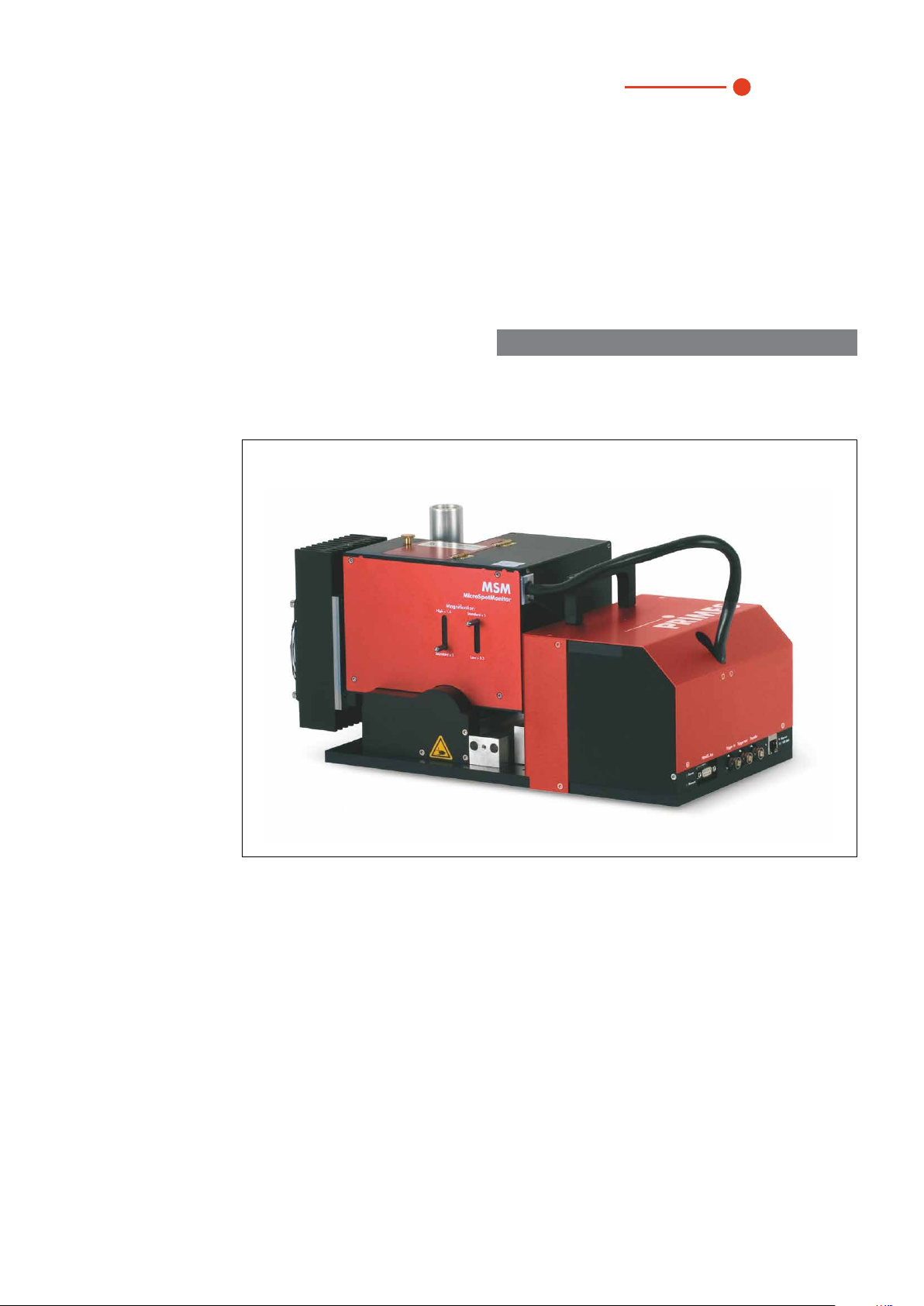
MicroSpotMonitor MSM
35,0(6
IMPORTANT!
READ CAREFULLY BEFORE USE.
KEEP FOR FUTURE USE.
Revision 01/2019 EN
3

MicroSpotMonitor MSM
35,0(6
Table of Contents
1 Basic safety instructions 9
2 Symbol explanations 11
3 About this operating manual 12
4 Conditions at the installation site 12
5 Introduction 13
5.1 System description .................................................................................................................13
5.2 Measuring principle .................................................................................................................14
5.3 Short overview installation .......................................................................................................15
6 Transport 16
6.1 Disassemble the transport lock ...............................................................................................16
6.2 Assemble the transport lock .................................................................................................... 17
7 Installation 17
7.1 Preparation and mounting position ..........................................................................................17
7.2 Manually aligning the MicroSpotMonitor MSM .........................................................................18
7.2.1 Important conditions for the position of the focused laser beam ................................ 18
7.2.2 Positioning the focused laser beam above the measuring objective ..........................19
7.2.3 Positioning the focused laser beam above the optional cyclone ................................20
7.3 Install the MicroSpotMonitor MSM...........................................................................................21
8 Connect cooling circuit (500W version only) 22
8.1 Water quality ...........................................................................................................................22
8.2 Water pressure ........................................................................................................................ 22
8.3 Humidity .................................................................................................................................. 23
8.4 Water connections and water flow rate ....................................................................................24
9 Electrical connection 25
9.1 Connections ............................................................................................................................ 25
9.2 Pin assignment .......................................................................................................................26
9.2.1 Power supply ............................................................................................................ 26
9.2.2 Inlet external trigger ..................................................................................................26
9.2.3 Outlet internal trigger .................................................................................................26
9.2.4 Outlet internal data-transfer signal ............................................................................. 26
9.3 Connection to the PC and connect power supply ...................................................................27
10 Status LEDs 28
11 Installation and configuration of the LaserDiagnosticsSoftware LDS 29
11.1 System requirements ..............................................................................................................29
11.2 Installing the software ..............................................................................................................29
11.3 Ethernet configuration .............................................................................................................30
11.3.1 Enter IP address .......................................................................................................30
11.3.2 Establishing a connection to PC (menu Communication > Free Communication) .. 31
11.3.3 Changing the standard IP address of the device (menu Communication > Free
Communication) ...................................................................................................... 32
4
Revision 01/2019 EN

MicroSpotMonitor MSM
35,0(6
12 Description of the LaserDiagnosticsSoftware LDS 34
12.1 Graphical user interface ........................................................................................................... 34
12.1.1 The menu bar ...........................................................................................................36
12.1.2 The toolbar ...............................................................................................................37
12.1.3 Menu overview .......................................................................................................... 38
12.2 File .......................................................................................................................................... 41
12.2.1 New (menu File > New) ............................................................................................ 41
12.2.2 Open (menu File > Open) ......................................................................................... 41
12.2.3 Close/Close all (menu File > Close/Close all) ........................................................... 41
12.2.4 Save (menu File > Save) ........................................................................................... 41
12.2.5 Save as (menu File > Save As) ................................................................................. 41
12.2.6 Export (menu File > Export) .....................................................................................41
12.2.7 Load measurement preferences (menu File > Load measurement preferences) ....42
12.2.8 Save measurement preferences (menu File > Save measurement preferences) .....42
12.2.9 Protocol (menu File > Protocol) ...............................................................................42
12.2.10 Print (menu File > Print) ...........................................................................................42
12.2.11 Print preview (menu File > Print preview) .................................................................42
12.2.12 Recently opened files (menu File > Recently opened Files) ..................................... 42
12.2.13 Exit (menu File > Exit) ............................................................................................... 42
12.3 Edit .........................................................................................................................................43
12.3.1 Copy (menu Edit > Copy) ......................................................................................... 43
12.3.2 Clear plane (menu Edit > Clear plane) .....................................................................43
12.3.3 Clear all planes (menu Edit > Clear all planes) ......................................................... 43
12.3.4 Change user level (menu Edit > Change User Level) ............................................... 43
12.4 Measurement ..........................................................................................................................44
12.4.1 Measuring environment (menu Measurement > Environment) ................................44
12.4.2 Sensor parameters (menu Measurement > Sensor parameter) .............................. 45
12.4.3 Beam find settings (menu Measurement > BeamFind Settings: Beamfind ........... 46
12.4.4 CCD info (menu Measurement > CCD Info) ............................................................47
12.4.5 CCD settings (menu Measurement > CCD Settings) ..............................................48
12.4.6 LQM adjustment (menu Measurement > LQM Adjustment) .................................... 50
12.4.7 Power measurement (menu Measurement > Power Measurement) .......................50
12.4.8 Single (menu Measurement > Single) ...................................................................... 50
12.4.9 Caustic measurement (menu Measurement > Caustic) ...........................................54
12.4.10 Start adjust mode (menu Measurement > Start Adjust mode) ................................ 55
12.4.11 Option (advanced user only) (menu Measurement > Option) ................................... 56
12.5 Presentation ............................................................................................................................58
12.5.1 False colors (menu Presentation > False colors) ..................................................... 59
12.5.2 False colors (filtered) (menu Presentation > False colors (filtered)) .........................60
12.5.3 Isometry (menu Presentation > Isometry) ...............................................................60
12.5.4 Isometry 3D (menu Presentation > Isometry 3D) ...................................................61
12.5.5 Review 86% or 2. moment (menu Presentation > Review (86%)/(2. moment)) .... 62
12.5.6 Caustic (menu Presentation > Caustic) .................................................................. 63
12.5.7 Raw beam (menu Presentation > Raw-beam) .......................................................67
12.5.8 Symmetry check (menu Presentation > SymmetryCheck) ...................................... 68
12.5.9 Fixed contour lines (menu Presentation > Fixed Contour Lines) ............................. 69
12.5.10 Variable contour lines (menu Presentation > Variable Contour Lines) ..................... 70
12.5.11 Graphical review (menu Presentation > Graphical Review) .....................................72
12.5.12 Systemstate (menu Presentation > Systemstate) ...................................................72
12.5.13 Evalution parameter view (menu Presentation > Evalution Parameter View) .......... 73
12.5.14 Evaluate document (menu Presentation > Evaluate doc) ........................................ 74
12.5.15 Color tables (menu Presentation > Color Tables) .................................................... 76
12.5.16 Toolbar (Menu Presentation > Toolbar) ...................................................................76
12.5.17 Position (menu Presentation > Position) .................................................................77
12.5.18 Evaluation (option) (menu Presentation > Evaluation) .............................................. 77
Revision 01/2019 EN
5

MicroSpotMonitor MSM
35,0(6
12.6 Communication ....................................................................................................................... 79
12.6.1 Rescan bus (menu Communication > Rescan bus) ................................................79
12.6.2 Free communication (menu Communication > Free Communication) ...................79
12.6.3 Scan device list (menu Communication > Scan device list) ................................... 80
12.7 Script (menu Script) ...............................................................................................................81
12.7.1 Editor (menu Script > Editor) ..................................................................................81
12.7.2 List (menu Script > List) .......................................................................................... 81
12.7.3 Python (menu Script > Python) ............................................................................... 81
13 Measurement 82
13.1 Safety instructions ................................................................................................................... 82
13.2 Selection and change of measuring objectives ........................................................................83
13.2.1 Selection of the measuring objective .........................................................................83
13.2.2 Exchanging the measuring objective .........................................................................85
13.2.3 Damage thresholds ...................................................................................................86
13.3 Prepare measurement .............................................................................................................89
13.3.1 Check list measurement settings...............................................................................89
13.3.2 Check list measurement settings...............................................................................89
13.4 Flowchart of a measurement ...................................................................................................90
13.4.1 Prepare measurement ...............................................................................................90
13.4.2 Set caustic limits ....................................................................................................... 90
13.4.3 Perform caustic measurement ..................................................................................91
13.5 Perform measurement settings in the LaserDiagnosticsSoftware LDS .....................................92
13.5.1 Sensor parameters (menu Measurement > Sensor parameter) .............................. 93
13.5.2 Measuring environment (menu Measurement > Environment) ................................94
13.5.3 Measurement settings (menu Measurement > Single) .............................................95
13.5.4 Caustic settings (menu Measurement > Caustic) .................................................... 96
13.5.5 CCD settings (menu Measurement > CCD Settings) ..............................................98
13.5.6 Option (advanced user only) (menu Measurement > Option) ................................. 100
13.5.7 CCD info (menu Measurement > CCD Info) ..........................................................101
13.5.8 Single measurement (menu Measurement > Single) ..............................................102
13.5.9 Caustic measurement (menu Measurement > Caustic) .........................................104
14 Troubleshooting 108
14.1 Error during a measurement ..................................................................................................108
14.2 No measurement signal at the MicroSpotMonitor MSM .........................................................108
15 Maintenance and service 109
15.1 Exchanging the protective window ........................................................................................109
15.1.1 Safety instructions ..................................................................................................109
15.1.2 Replacing the protective window ............................................................................110
15.1.3 Replacing the protective window for cyclone ...........................................................111
16 Storage 112
17 Measures for the product disposal 112
18 Declaration of conformity 113
19 Technical data 114
6
Revision 01/2019 EN

MicroSpotMonitor MSM
35,0(6
20 Dimensions 116
21 Appendix 117
21.1 Insert fixed OD filter (option) in the inspection chamber .........................................................117
21.2 File “laserds.ini” – an Example ...............................................................................................118
21.3 Description of the MDF file format .........................................................................................119
21.4 Optical components .............................................................................................................. 120
21.4.1 Measuring objective ................................................................................................ 121
21.4.2 Fixed filter and filter wheel .......................................................................................126
21.4.3 Beam path extension (BPE) ....................................................................................127
21.4.4 Alignment objective (JO) .......................................................................................... 127
21.4.5 Absorber ................................................................................................................. 128
21.4.6 Trigger diode ........................................................................................................... 128
21.4.7 Charge-coupled device sensor (CCD sensor) .......................................................... 128
21.5 Measuring pulsed irradiation ................................................................................................. 132
21.5.1 Measuring configuration selection ...........................................................................134
21.5.2 Influence of the pulse parameters on the integration time control ............................134
21.5.3 Examples for triggered measuring mode .................................................................138
21.5.4 Summary ................................................................................................................ 139
22 Basis of laser beam diagnosis 140
22.1 Laser beam parameter .......................................................................................................... 140
22.1.1 Rotationally symmetric beams.................................................................................141
22.1.2 Non rotationally symmetric beams ..........................................................................142
22.2 Calculation of beam data ......................................................................................................143
22.2.1 Determination of the zero level ................................................................................143
22.2.2 Determination of the beam position ......................................................................... 144
22.2.3
22.2.4 Radius determination with the method of the 86% power inclusion ....................... 145
22.2.5 Further radius definitions (option).............................................................................146
22.3 Measurement errors ..............................................................................................................147
22.3.1 Error in determining zero level .................................................................................147
22.3.2 Saturating the signal ...............................................................................................147
22.3.3 Errors from incorrect measurement window size ..................................................... 148
Radius determination with the 2. moment method of the power density distribution ..
144
Revision 01/2019 EN
7

MicroSpotMonitor MSM
35,0(6
PRIMES - The Company
PRIMES manufactures measuring devices used to analyze laser beams. These devices are employed for
the diagnostics of high-power lasers ranging from CO
length range from infrared through to near UV is covered, offering a wide variety of measuring devices to
determine the following beam parameters:
• Laser power
• Beam dimensions and position of an unfocused beam
• Beam dimensions and position of a focused beam
• Beam quality factor M²
PRIMES is responsible for both the development, production, and calibration of the measuring devices. This
guarantees optimum quality, excellent service, and a short reaction time, providing the basis for us to meet all
of our customers’ requirements quickly and reliably.
lasers and solid-state lasers to diode lasers. A wave-
2
PRIMES GmbH
Max-Planck-Str. 2
64319 Pfungstadt
Germany
Tel +49 6157 9878-0
info@primes.de
www.primes.de
8
Revision 01/2019 EN

MicroSpotMonitor MSM
35,0(6
1 Basic safety instructions
Intended Use
The MicrsoSpotMonitor MSM has been designed exclusively for measurements carried out in or near the
optical path of high-power lasers. Please observe and adhere to the specifications and limit values given
in chapter19, „Technical data“, on page114. Other uses are considered to be improper. The information
contained in this operating manual must be strictly observed to ensure proper use of the device.
Using the device for unspecified use is strictly prohibited by the manufacturer. By usage other than intended
the device can be damaged or destroyed. This poses an increased health hazard up to fatal injuries. When
operating the device, it must be ensured that there are no potential hazards to human health.
The device itself does not emit any laser radiation. During the measurement, however, the laser beam is
guided onto the device which causes reflected radiation (laser class 4). That is why the applying safety regulations are to be observed and necessary protective measures need to be taken.
Observing applicable safety regulations
Observing applicable safety regulations
Please observe valid national and international safety regulations as stipulated in ISO/CEN/TR standards as
well as in the IEC-60825-1 regulation, in ANSI Z 136 “Laser Safety Standards” and ANSI Z 136.1 “Safe Use
of Lasers”, published by the American National Standards Institute, and additional publications, such as the
“Laser Safety Basics”, the “LIA Laser Safety Guide”, the “Guide for the Selection of Laser Eye Protection”
and the “Laser Safety Bulletin”, published by the Laser Institute of America, as well as the “Guide of Control
of Laser Hazards” by ACGIH.
Necessary safety measures
DANGER
Serious eye or skin injury due to laser radiation
During the measurement the laser beam is guided on the device, which causes scattered or
directed reflection of the laser beam (laser class 4). The reflected beam is usually not visible.
Please take the following precautions.
X
If people are present within the danger zone of visible or invisible laser radiation, for example near laser
systems that are only partly covered, open beam guidance systems, or laser processing areas, the following
safety measures must be implemented:
• Please wear safety goggles adapted to the power, power density, laser wave length and operating
mode of the laser beam source in use.
• Depending on the laser source, it may be necessary to wear suitable protective clothing or protective
gloves.
• Protect yourself from direct laser radiation, scattered radiation, and beams generated from laser radiation
(by using appropriate shielding walls, for example, or by weakening the radiation to a harmless level).
• Use beam guidance or beam absorber elements that do not emit any hazardous substances when they
come in to contact with laser radiation and that can withstand the beam sufficiently.
• Install safety switches and/or emergency safety mechanisms that enable immediate closure of the laser
shutter.
• Ensure that the device is mounted securely to prevent any movement of the device relative to the beam
axis and thus reduce the risk of scattered radiation. This in the only way to ensure optimum performance
during the measurement.
Revision 01/2019 EN
9

MicroSpotMonitor MSM
35,0(6
Employing qualified personnel
The device may only be operated by qualified personnel. The qualified personnel must have been instructed
in the installation and operation of the device and must have a basic understanding of working with highpower lasers, beam guiding systems and focusing units.
Conversions and modifications
The device must not be modified, neither constructionally nor safety-related, without our explicit permission.
The device must not be opened e.g. to carry out unauthorized repairs. Modifications of any kind will result in
the exclusion of our liability for resulting damages.
Liability disclaimer
The manufacturer and the distributor of the measuring devices do not claim liability for damages or injuries
of any kind resulting from an improper use or handling of the devices or the associated software. Neither the
manufacturer nor the distributor can be held liable by the buyer or the user for damages to people, material
or financial losses due to a direct or indirect use of the measuring devices.
10
Revision 01/2019 EN
MicroSpotMonitor MSM
35,0(6
2 Symbol explanations
The following symbols and signal words indicate possible residual risks:
DANGER
Means that death or serious physical injuries will occur if necessary safety precautions are not
taken.
WARNING
Means that death or serious physical injuries may occur if necessary safety precautions are not
taken.
CAUTION
Means that minor physical injury may occur if necessary safety precautions are not taken.
NOTICE
Means that property damage may occur if necessary safety precautions are not taken.
The following symbols indicating requirements and possible dangers are used on the device:
Hand injuries warning
Components susceptible to ESD
Read and observe the operating instructions and safety guidelines before startup!
Further symbols that are not safety-related:
Here you can find useful information and helpful tips.
Revision 01/2019 EN
With the CE designation, the manufacturer guarantees that its product meets the requirements of
the relevant EC guidelines.
Call for action
X
11

MicroSpotMonitor MSM
35,0(6
3 About this operating manual
This documentation describes how to work with the MicroSpotMonitor MSM and operate it with the LaserDiagnosticsSoftware LDS 2.98.
The software description includes a brief introduction on using the device for measurements.
This operating manual describes the software version valid at the time of printing.
Since the user software is continuously being developed further, the supplied data medium may
have a different version number. Correct functioning of the device is, however, still guaranteed with
the software.
Should you have any questions, please specify the software version installed on your device. The software
version can be found under the following menu item: Help > About LaserDiagnosticsSoftware.
Fig. 3.1: Information regarding the current software version
4 Conditions at the installation site
• The device must not be operated in a condensing atmosphere.
• The ambient air must be free of organic gases.
• Protect the device from splashes of water and dust.
• Operate the device in closed rooms only.
12
Revision 01/2019 EN

MicroSpotMonitor MSM
35,0(6
5 Introduction
5.1 System description
The MicroSpotMonitor MSM determines beam parameters of focused laser beams with medium powers up
to 200W in a range between 20micro meters and one millimeter directly in the processing zone.
The air-cooled system depicts the laser beam, which is attenuated by different beam splitter and neutral
density filters, on a CCD sensor. On the basis of the determined beam distribution of a plane, the beam position as well as the beam radius can be derived. By means of the integrated z-axis and the measurement at
different positions of the laser beam the described beam parameters are determined and logged.
The measuring objectives of the MicroSpotMonitor MSM are selected individually, depending on the beam
source that is supposed to be measured. In this regard, the wavelength (248 up to 1 090 nm) as well as the
magnification (3.3:1, 5:1, 10:1), which is determined by the focus diameter, are the essential parameters.
The dynamic range of the integrated CCD sensor is amplified to more than 130dB via an irradiation time
control, which enables caustic measurements over more than four Rayleigh lengths, as demanded in the
standard ISO11146.
Optionally, the MicroSpotMonitor MSM can be equipped with a filter wheel with neutral density filters (OD1
to OD5). This filter wheel enables the measurement of power densities between several W/cm² up to several
MW/cm² without having to modify the system.
Cyclone (option)
Knurled screw
Absorber
Ventilator
Traversing motor
Transport lock
Beam entrance
to filter wheel (option) and fixed OD-filter (option)
Access (inspection chamber)
Lever to adjust the
magnification
(option)
Beam path extension (BPE)
Standard
Fig. 5.1: Components of the MicroSpotMonitor MSM
Revision 01/2019 EN
Alignment objective (AO)
13

MicroSpotMonitor MSM
35,0(6
5.2 Measuring principle
The MicroSpotMonitor MSM is a camera-based measuring system. Depending on the application, up to 7
different optical components can be in the beam path. The purpose and functioning of individual components is described in chapter21.4, „Optical components“, on page120.
Laser beam
Upper limit
Measuring plane
Lower limit
Measuring
objective
Absorber
Prisms
Fixed OD-filter (option)
Alignment objective (AO)
CCD sensor
Fig. 5.2: Optomechanical design
Mirrors
Absorber
Trigger
Filter wheel (option)
Beam path extension (BPE)
14
Revision 01/2019 EN

MicroSpotMonitor MSM
35,0(6
5.3 Short overview installation
1. Taking safety precautions Chapter 1 on page 9
2. Transport
• Disassemble the transport lock
3. Installation
• Make preparations
• Set the installation position
• Align the device manually
• Mount the device firmly
4. Connect the water-cooling (500 W version only)
• Connection diameter
• Observe flow rate
5. Electrical connection
• Establish voltage supply
Chapter 6 on page 16
Chapter 7 on page 17
Chapter 8 on page 22
Chapter 9 on page 25
6. Connect with the PC
• Via Ethernet or LAN
7. Installing the LaserDiagnosticsSoftware LDS on the PC
• Software is part of the scope of delivery
• Connect the MicroSpotMonitor MSM with the LaserDiagnosticsSoftware LDS
8. Measure
• Follow the safety instructions
• Select and insert the measuring objective
• Observe damage thresholds
• Perform measurement
Chapter 9.3 on page 27
Chapter 11 on page 29
Chapter 13 on page 82
Revision 01/2019 EN
15
35,0(6
6 Transport
WARNING
Risk of injury when lifting or dropping the device
Lifting and positioning heavy devices can, for example, stress intervertebral disks and cause
chronic changes to the lumbar or cervical spine. The device may fall.
Use a lifting device to lift and position the device.
X
NOTICE
Damaging/destroying the device
Optical components may be damaged if the device is subjected to hard shocks or is allowed
to fall.
Handle the measuring device carefully when transporting or installing it.
X
To avoid contamination, close the measuring objective with the cover provided.
X
Only transport the device in the original PRIMES transport box (option).
X
MicroSpotMonitor MSM
6.1 Disassemble the transport lock
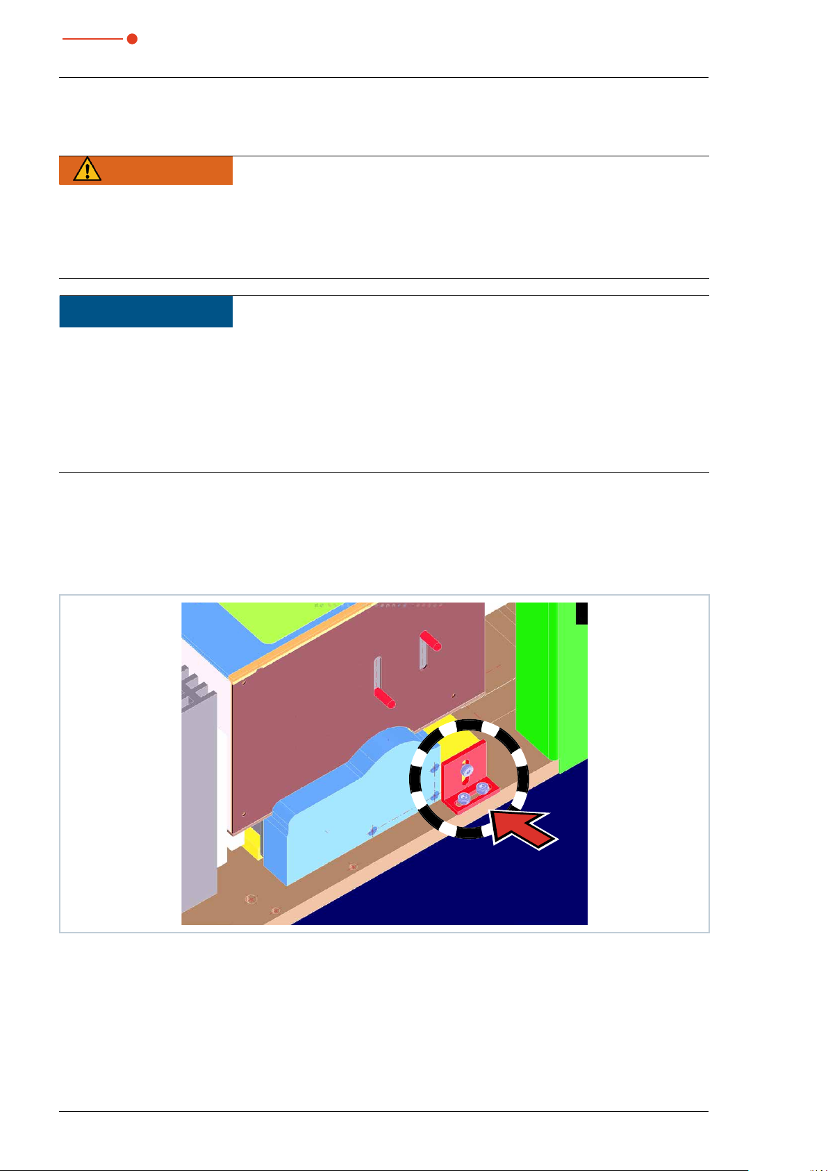
After unpacking the device, the transport lock has to be removed first. The transport lock secures the linear
actuator of the z-axis. It is located on the bottom plate and is fastened by means of 3 screws (see Fig. 6.1 on
page 16).
Fig. 6.1: Position of the transport lock
16
Revision 01/2019 EN

MicroSpotMonitor MSM
35,0(6
6.2 Assemble the transport lock
NOTICE
Damaging/destroying the device
The device must only be transported with a mounted transport lock.
Keep the transport lock for future use.
X
Before transportation, move the MicroSpotMonitor MSM into the parking position (see chapter12.5.17, „Position (menu Presentation > Position)“, on page77) and mount the transport lock.
7 Installation
7.1 Preparation and mounting position
Check the space available before mounting the device, especially the required space for the connection
cables and the movement range of the z-axis (see chapter20, „Dimensions“, on page116). The device
must be set up so that it is stable and fastened with screw (see chapter 7.3 on page 21).
The MicroSpotMonitor MSM is designed to operate in a horizontal position with a beam incidence from
above. With an optional side plate (order no. 801-004-060), operation with horizontal beam incidence is also
possible.
NOTICE
Damaging/destroying the device
Obstacles in the movement range of the MicroSpotMonitor MSM can lead to collisions and
damage the device.
Keep the movement range free of obstacles (cutting nozzle, pressure rolls, etc.).
X
Revision 01/2019 EN
17
MicroSpotMonitor MSM
35,0(6
7.2 Manually aligning the MicroSpotMonitor MSM
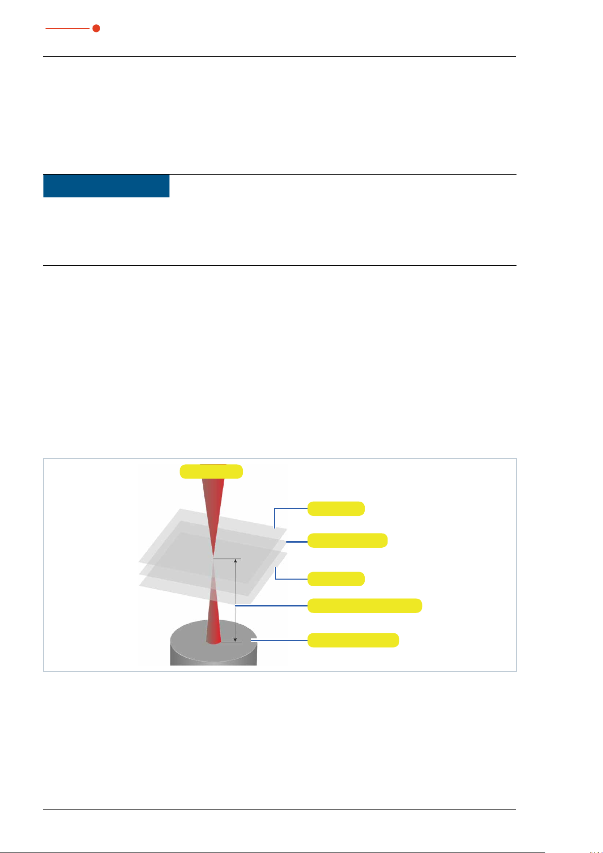
7.2.1 Important conditions for the position of the focused laser beam
Due to the imaging characteristics of the measuring objective (see chapter21.4.1, „Measuring objective“, on
page121) it is necessary for the laser beam focus to be positioned in a certain range above the measuring
objective.
NOTICE
Damaging/destroying the device
The focus has to be in a defined range with reference to the measuring objective. In case it
is too close or too distant, the optics might be damage in case of high beam intensities.
Use the enclosed alignment tool for the alignment.
X
The size of the range in which the focus is to be positioned before the first measurement depends on the
chosen measuring objective, the used wavelength and the type of focusing. The measurement range lies
within an upper and a lower limit.
Upper limit
If the focus is located too high above the measuring objective, a focus on the image-sided beam path can
develop. Together with too high beam intensities, the optics might be damaged.
Measuring plane
The beam distribution of the measuring plane is displayed on the CCD sensor.
Lower limit
If the focus is too close to the measuring objective, it can – depending on the type of focusing and the power
used – damage the entrance lens.
Laser beam
Upper limit
Measuring plane
Lower limit
Measuring plane distance
Measuring objective
Fig. 7.1: Measuring range of the MicroSpotMonitor MSM
18
Revision 01/2019 EN

MicroSpotMonitor MSM
35,0(6
7.2.2 Positioning the focused laser beam above the measuring objective
The measuring plane distance equals the distance of the measuring plane from the upper corner of the measuring objective or the protective glass.
In order to be able to align the MicroSpotMonitor MSM beneath the laser, an associated alignment tool is
provided with each measuring objective. By means of this alignment tool and a pilot laser beam, you can
position the device with the necessary accuracy.
1. Place the alignment tool directly on the measuring objective (see Fig. 7.2 on page 19) or on the protective window holder on the measuring objective (see Fig. 7.3 on page 19).
• The upper edge of the measuring objective corresponds to the z position of the measuring plane.
• When using a protective window with a thickness of 1.5mm, the measuring plane moves upwards by
approx. 500µm.
2. Turn on the pilot laser. If the laser hits the marking in the alignment tool vertically, it is displayed centrally
on the CCD sensor.
Marking in the alignment tool
10x
Fig. 7.2: Alignment tools for direct placement on the measuring objective
Marking in the alignment tool
10x 5x 3.3x
Fig. 7.3: Alignment tools for placement on the protective window holder on the measuring objective
5x
3.3x
Revision 01/2019 EN
19
MicroSpotMonitor MSM
35,0(6
The measuring plane distance equals the distance of the imaging plane from the upper corner of the measuring objective. It does not only depend on the beam path (standard, beam path extension BPE, alignment
objective AO) but also on the wavelength (see Tab. 7.1 on page 20).
When using a protective window with a thickness of 1.5mm, the measuring plane moves upwards
by approx. 500µm.
Measuring ob-
jective MOB
3.3x
1 064nm
532nm
355nm
5x
1 064nm
532nm
355nm
10x
1 064nm
532nm
355nm
Tab. 7.1: Measuring plane distances
NA limit
values
1
0.1
0.09
0.19
0.18
0.14
0.24
0.24
0.17
Typ. magnification Measuring plane distance in mm
Standard BPE AO Standard BPE AO
3.12
3.23
3.36
4.96
5.15
5.35
8.84
9.17
9.62
5.65
5.81
6.02
8.31
8.6
8.92
14.39
14.91
15.6
1.12
1.11
*)
1.63
1.59
*)
2.77
2.72
*)
73
70.5
67.3
51.1
49.3
47.2
29.9
-
-
64.6
62.6
60.1
47.1
45.7
43.8
27.9
-
-
63.7
61.5
57.7
46.7
45.1
42.7
27.6
-
-
*) Only suitable for adjustment
Due to the production tolerances, the values of the measuring plane distance contain a deviation of
±800µm. However, it is possible to have the measuring distance of the measuring objective calibrated to
±50µm (TCP calibration).
7.2.3 Positioning the focused laser beam above the optional cyclone
For measuring objectives with a cyclone or a protective window special alignment aids are provided.
Marking in the alignment tool
Alignment tool
Cyclone with disassembled protective window
holder and attached alignment tool
Fig. 7.4: Alignment tool for an optional cyclone using the example of a measuring objective with 3.3x magnification
Cyclone with mounted protective window
holder and removed alignment tool
20
Revision 01/2019 EN
MicroSpotMonitor MSM
35,0(6
7.3 Install the MicroSpotMonitor MSM
DANGER
Serious eye or skin injury due to laser radiation
If the device is moved from its calibrated position, increased reflected radiation
(laser class 4) may result during measuring operation.
When mounting the device, please ensure that it cannot be moved, neither due to an unin-
X
tended push or a pull on the cables and hoses.
150166.6
187.5157.5
2x Ø11
2x Ø6.6
4x Ø 6.6 Ø11
202
157.5 187.5
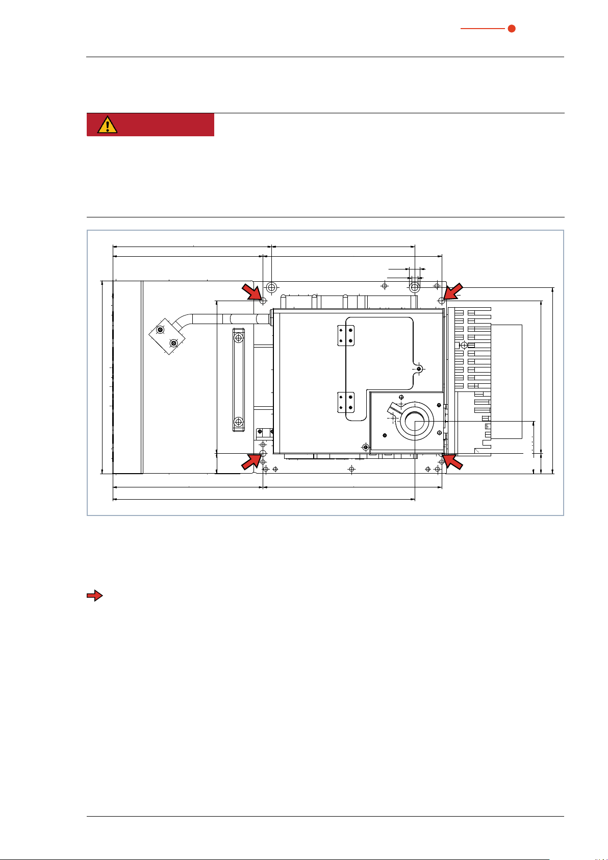
Fig. 7.5: Fastening bores, view from above
For the installation onto a holder provided by the customer, there are four mounting holes Ø6,6mm in the
bottom plate. We recommend screws M6 of the strength class 8.8 and a tightening torque of 20N∙m.
4 Mounting holes Ø6,6mm
160
21
316.6 +12
160
54.8 ±0.5
21
194.8
Revision 01/2019 EN
21

35,0(6
8 Connect cooling circuit (500W version only)
DANGER
Fire hazard; Damage/Destruction of the device due to overheating
If there is no water cooling or a water flow rate which is insufficient, there is a danger of
overheating, which can damage the device or set it on fire.
Operate the device with a connected water cooling and a sufficient water flow rate only.
X
8.1 Water quality
NOTICE
Damage/Destruction of the device due to different chemical potentials
The parts of the device which get in contact with cooling water consist of copper, brass or
stainless steel. Connecting the unit to a colling curcuit containing aluminum components
may cause corrosion of the aluminum due to the different chemical potentials.
Do not connect the device on a cooling circuit in which aluminum components are installed.
X
MicroSpotMonitor MSM
• The device can be operated with tap water as well as demineralized water.
• Do not operate the device on a cooling circuit containing additives such as anti-freeze.
• Do not operate the device on a cooling circuit in which aluminum components are installed. Especially
when it comes to the operation with high powers and power densities, it may otherwise lead to corrosion
in the cooling circuit. In the long term, this reduces the efficiency of the cooling circuit.
• Should the cooling fail, the device can withstand the laser radiation for a few seconds. In this case,
please check the device as well as the water connections for damages.
• Large dirt particles or teflon tape may block internal cooling circuits. Therefore, please thoroughly rinse
the system before connecting it.
8.2 Water pressure
Normally, 2 bar primary pressure at the entrance of the absorber are sufficient in case of an unpressurized
outflow.
NOTICE
Damage/Destruction of the device due to overpressure
The maximum permissible water inlet pressure must not exceed 4bar.
X
22
Revision 01/2019 EN

MicroSpotMonitor MSM
35,0(6
8.3 Humidity
• The device must not be operated in a condensing atmosphere. The humidity has to be considered in
order to prevent condensates within and outside the device.
• The temperature of the cooling water must not be lower than the dew point (see Tab. 8.1 on page 23).
NOTICE
Damage/Destruction of the device due to condensing water
Condensation water inside of the objective will lead to damage.
Mind the dew-point in Tab. 8.1 on page 23.
X
Do only cool the device during the measuring operation. We recommend starting the cooling approx. 2minutes before the measurement and terminating it approx. 1minute after the measurement.
40
35
30
25
20
15
10
Cooling water temperature in °C
5
0
Tab. 8.1: Dew point diagram
Example
Air temperature: 22°C
Relative humidity: 60%
0 5 10 15 20 25 30 35 40
Air temperature in °C
100
80
70
60
50
40
30
20
Relative humidity in %
10
The cooling water temperature cannot fall below 14°C.
Revision 01/2019 EN
23

MicroSpotMonitor MSM
35,0(6
8.4 Water connections and water flow rate
Connection diameter Recommended flow rate Minimum flow rate
PE hoses 12mm 1.5l/min (1l/(min · kW) Not lower than 1.0l/min
Tab. 8.2: Water connections and water flow rate
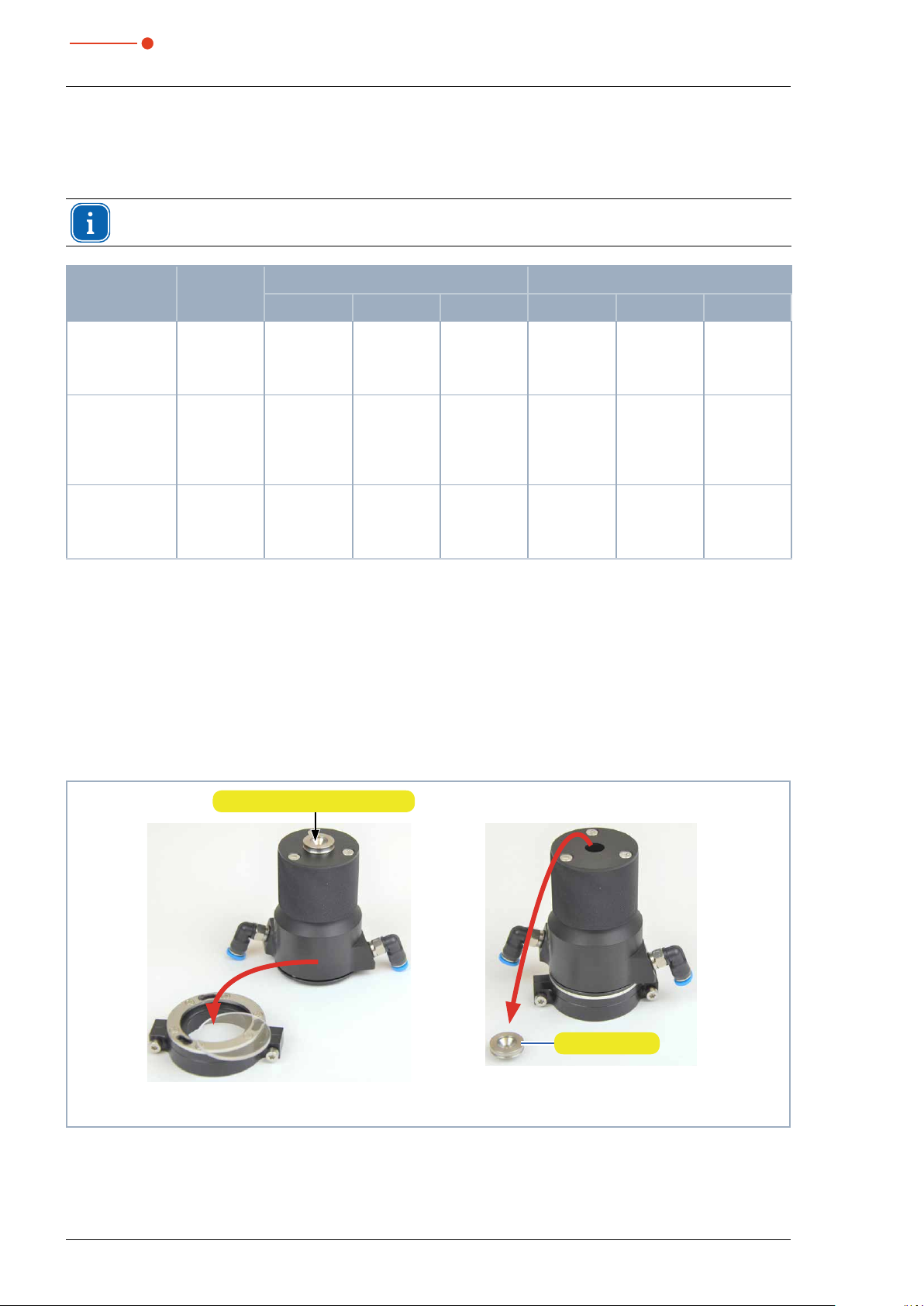
Remove the sealing plugs of the water connections
Release ring
1. Push
2. Pull
Fig. 8.1: Remove the sealing plugs of the water connections
1. Please push down the release ring of the connection
and pull out the plug with your free hand.
2. Remove the sealing plugs of the water connections and
keep it in a save place.
3. Close the flow line (Water In) and the return flow (Water
Out) of the device, by inserting the hose as far as possible (approx. 2cm deep).
24
Revision 01/2019 EN

MicroSpotMonitor MSM
35,0(6
9 Electrical connection
The MicroSpotMonitor MSM requires a supply voltage of 24V±5% (DC) for the operation. A suitable power
supply with an adapter is included in the scope of delivery. Please use only the provided connection lines.
Please ensure that all electrical connections have been established and switch the device on before
starting the LaserDiagnosticsSoftware LDS.
The MicroSpotMonitor MSM serves as a dongle for the software on the PC in order to enable certain software functions.
9.1 Connections
On/off switch
RS485 PRIMES bus
D-Sub socket9 pole
(Power supply connection)
Fig. 9.1: Connections
Revision 01/2019 EN
Input
external trigger
BNC
Output
internal trigger
BNC
Ethernet
Outlet data transfer signal
25

35,0(6
9.2 Pin assignment
9.2.1 Power supply
D-Sub socket, 9-pin (view: connector side)
MicroSpotMonitor MSM
Pin Function
1 GND
15
69
Tab. 9.1: D-Sub socket RS485
2 RS485 (+)
3 +24 V
4 Trigger RS485 (+)
5 Not assigned
6 GND
7 RS485 (–)
8 +24 V
9 Trigger RS485 (–)
9.2.2 Inlet external trigger
BNC connector (view: connector side)
Pin Function
1 +5 V (Trigger signal)
1
2
Fig. 9.2: Connection socket inlet for an external trigger in the connection panel
2 GND
9.2.3 Outlet internal trigger
BNC connector (view: connector side)
Pin Function
1 +5 V (Trigger signal)
1
2
Fig. 9.3: Connection socket outlet for the internal trigger in the connection panel
2 GND
9.2.4 Outlet internal data-transfer signal
BNC connector (view: connector side)
Pin Function
1 +5 V (Trigger signal)
1
2
Fig. 9.4: Connection socket outlet for the internal data-transfer signal in the connection panel
2 GND
26
Revision 01/2019 EN
MicroSpotMonitor MSM
35,0(6
9.3 Connection to the PC and connect power supply
NOTICE
Damage/Destruction of the device
When the electrical cables are disconnected during operation (when the power supply is applied), voltage peaks occur which can destroy the communication components of the measuring device.
Please turn off the PRIMES power supply before disconnecting the cables.
X
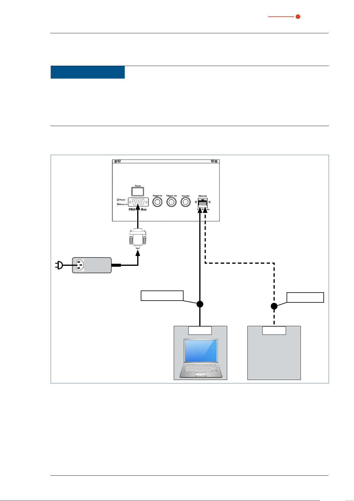
1. Connect the device with the PC via a crossover cable or with the network via a patch cable.
2. Use the adapter to connect the power supply to the 9-pin D-sub socket (RS485) of the device.
MSM
Adapter
PRIMES Power Supply
Crossover cable
Ethernet
PC
Fig. 9.5: Connection via Ethernet with a PC or a local network
or
Patch cable
Ethernet
LAN
Revision 01/2019 EN
27

35,0(6
10 Status LEDs
The device has two status LEDs.
Bezeichnung Farbe Bedeutung
Power Green The power supply is switched on
Measuring Yellow A measurement is running
Tab. 10.1: Description of the status LEDs on the MicroSpotMonitor MSM
Power supply
MicroSpotMonitor MSM
Measuring mode
Fig. 10.1: Status LEDs on the MicroSpotMonitor MSM
28
Revision 01/2019 EN

MicroSpotMonitor MSM
35,0(6
11 Installation and configuration of the LaserDiagnosticsSoftware LDS
In order to operate the measuring device, the PRIMES LaserDiagnosticsSoftware LDS has to be installed on
the computer. The program can be found on the enclosed medium.
You will find the latest version on the PRIMES website at: https://www.primes.de/en/support/downloads/
software.html.
11.1 System requirements
Operating system: Windows® 7/10
Processor: Intel® Pentium® 1GHz (or comparable processor)
Free disc space: 15 MB
Monitor: 19“ screen diagonal is recommended, resolution at least 1024x768
LDS-Version: 2.98 or higher
11.2 Installing the software
The installation of the software is menu driven and is effected by means of the enclosed medium. Please
start the installation by double-clicking the file “Setup LDS v.X.X.exe” (X = placeholder for version number)
and follow the instructions.
Fig. 11.1: Setup of the PRIMES LaserDiagnosticsSoftware LDS
If not stipulated differently, the installation software stores the main program “LaserDiagnosticsSoftware.
exe” in the directory “Programs/PRIMES/LDS”. Moreover, the settings file “laserds.ini” is also copied into this
directory. In the file “laserds.ini” the setting parameters for the PRIMES measuring devices are stored.
Revision 01/2019 EN
29

35,0(6
11.3 Ethernet configuration
11.3.1 Enter IP address
The MicroSpotMonitor MSM has a fixed IP address that is specified on the type plate:
• If the MicroSpotMonitor MSM is connected directly to the PC, enter the fixed IP address in the
menu Communication > Free Communication (see chapter 11.3.2 on page 31).
• If the MicroSpotMonitor MSM is connected over a network, the MicroSpotMonitor MSM will
spend about one minute pulling up a variable IP address in the network.
You can read off this variable IP address with the provided software, “PrimesFindlp” and enter it
into the Communication > Free Communication (see chapter 11.3.2 on page 31)
• If you want to connect the MicroSpotMonitor MSM to the network using the fixed IP address,
first turn on the MicroSpotMonitor MSM and then connect the network cable to the MicroSpotMonitor MSM. Then enter the fixed IP address in the menu Communication > Free Commu-
nication (see chapter 11.3.2 on page 31).
The standard IP address of the MicroSpotMonitor MSM is:
IP Address: 192.168.116.84
Subnet mask: 255.255.255.0
MicroSpotMonitor MSM
The PC must also have an IP address in the same subnet, for example:
IP Address: 192.168.116.XXX
Subnet mask: 255.255.255.0
The first three blocks of the IP address must match the IP of the MicroSpotMonitor MSM.
Type plate MSM
192
168
255
255
116
255800
Fig. 11.2: Ethernet configuration in the dialogue window Ethernet
30
Revision 01/2019 EN
MicroSpotMonitor MSM
35,0(6
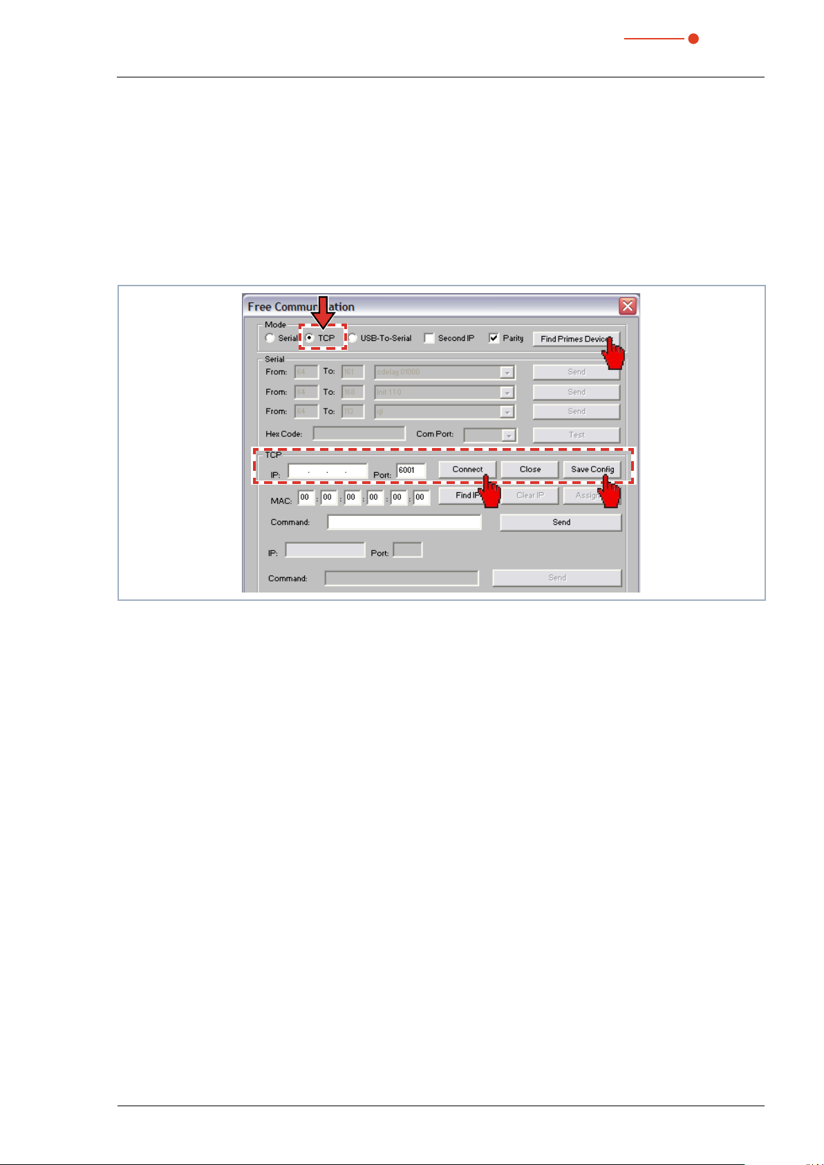
11.3.2 Establishing a connection to PC (menu Communication > Free Communication)
1. Please start the LaserDiagnosticsSoftware LDS (see chapter 12 on page 34).
2. Open the dialogue window Communication > Free Communication.
3. Choose in the field “Mode” TCP (the option “Second IP” must not be activated!).
4. Enter in the field “TCP” the IP Address.
5. Click on the Connect button (“connected” appears in the bus monitor).
6. Click on the Find Primes Devices button.
7. Click on the Safe Config button (the configuration is saved and does not need to be re-entered when
starting the LaserDiagnosticsSoftware LDS again).
192 168 116 84
Fig. 11.3: Establishing a connection in the dialogue window Free Communication
Revision 01/2019 EN
31
MicroSpotMonitor MSM
35,0(6
11.3.3 Changing the standard IP address of the device (menu Communication > Free Communication)
If the fixed IP address of the MicroSpotMonitor MSM conflicts with another device bearing the same IP address on the network, the fixed IP address of the MicroSpotMonitor MSM can be changed.
NOTICE
Device malfunction due to erroneous entries
While changing the IP address, it is possible that another EE cell might be overwritten by a
mistype, for example, and the MicroSpotMonitor MSM could thus be rendered unusable.
Only very skilled users should attempt to change the IP address.
X
You can change the preset IP address in the menu Communication > Free communication by means of
the following commands:
IP-address
(Sample address)
Commands
Tab. 11.1: Changing the IP address
In this case xyz are place holders of the four IP-address bytes (values 1 - 254) which always have to be
entered with three digits!
For example, the number 84 has to be entered like this: 084.
For reasons of clarity the symbol marks a space.
192. 168. 116. 85
se0328wxyz se0329xyz se0330xyz se0331xyz
32
Revision 01/2019 EN
MicroSpotMonitor MSM
35,0(6
Example: You will change the IP address from 192.168.116.85 to 192.168.116.86.
1. Please start the LaserDiagnosticsSoftware LDS (see chapter 12 on page 34).
2. Open the dialogue window Communication > Free Communication.
3. Choose in the field “Mode” TCP (the option “Second IP” must not be activated!).
4. Enter the current IP address in the “TCP” field.
5. Click on the Connect button (“connected” appears in the bus monitor).
6. Activate the check box Write bus protocol (the protocol can be helpful in case of problems):
• The protocol is stored in the installation index of the LaserDiagnosticsSoftware LDS.
• The file name is buspro.log.YYYY/MM/DD (YYYY/MM/DD = date file was created).
7. Enter the following in the field “Command”: se0331086
(please make sure that the blank character is entered correctly).
8. Click on the Send button and wait for the confirmation in the bus monitor
(see Fig. 11.4 on page 33 „-> Adr:0331 Wert: 086“)
9. Please turn off the device and turn it on again. After the restart the IP-address is updated.
se0331 086
Adr: 0331 Wert:086
Confirmation
Fig. 11.4: Changing the IP address in the dialogue window Free Communication
Revision 01/2019 EN
33
MicroSpotMonitor MSM
35,0(6
12 Description of the LaserDiagnosticsSoftware LDS
The LaserDiagnosticsSoftware LDS is the control centre for all PRIMES measuring devices which measures
the beam distribution as well as focus geometries by means of which the beam propagation characteristics
can be determined.
The LaserDiagnosticsSoftware LDS includes all functions necessary for the control of measurements and
displays the measuring results graphically.
Moreover, the systems uses the measured data to carry out an evaluation in order to give the operator of the
beam diagnosis an information regarding the reliability of the measuring results.
Please do not start the LaserDiagnosticsSoftware LDS before all devices are connected and turned
on.
Please start the program by double-clicking the LDS symbol
link.
in the new start menu group or the desktop
12.1 Graphical user interface
Firstly, a start window is opened in which you can choose, whether you would like to measure or whether
you would just like to depict an existing measurement (factory setting “measurement”).
Fig. 12.1: Start window of the LaserDiagnosticsSoftware LDS
After the detection of the connected device, the graphical user interface and several important dialogue
windows are opened.
In order to ensure that corresponding information can be assigned quickly, special markups for menu items,
menu paths and texts of the user interface will be used in the following chapters.
Markup Description
Text Marks menu items.
Text1 > Text2 Marks the navigation to certain menu items.
Text Marks buttons, options and fields.
Fig. 12.2: Special markups for menu items, menu paths and texts
34
Example: Dialogue window Sensor parameters
The Order of the menus is depicted by means of the Sign “>”
Example: Presentation > Caustic
Example: With the button Start
Revision 01/2019 EN
MicroSpotMonitor MSM
35,0(6
The graphical user interface mainly consists of the menu as well as the toolbar by means of which different
dialogue or display windows can be called up.
Menu bar
Tool bar
Dialogue window
Fig. 12.3: The main elements of the user interface
It is possible to open several measuring and dialogue windows simultaneously. In this case, windows that are
basically important (for the measurement or the communication) remain in the foreground. All other dialog
windows fade into the background as soon as a new window opens.
Fig. 12.4: The main dialogue windows
Revision 01/2019 EN
35

35,0(6
12.1.1 The menu bar
In the menu bar, all main and sub menus offered by the program can be opened.
MicroSpotMonitor MSM
Fig. 12.5: Menu bar
36
Revision 01/2019 EN

MicroSpotMonitor MSM
35,0(6
12.1.2 The toolbar
By clicking the symbols in the toolbar, the following program menus can be opened.
File administration Notation File selection Plane selection
1 2 3 4 5 6 7 8 9 10 11
Fig. 12.6: Symbols in the toolbar
1 - Create a new data record
2 - Open an existing data record
3 - Save the current data record
4 - Open the isometric view of the selected data record
5 - Open the variable contours line view
6 - Open review (86%)
7 - Open false color depiction
8 - Caustic presentation 2D
9 - List with all data records opened
10 - Display of the selected measuring plane
11 - Display of the measuring devices available for the bus by means of graphical symbols
All measuring results are always written into the document selected in the toolbar.
It is only possible to display documents chosen here. After opening, the data set has to be explicitly selected.
Revision 01/2019 EN
37

35,0(6
12.1.3 Menu overview
File
New Opens a new file for the measuring data
Open Opens a measuring file with the extensions “.foc” or “.mdf”
Close Closes the file selected in the toolbar
Close all Closes all files opened
Save Saves the current file in foc- or mdf format
MicroSpotMonitor MSM
Save as Opens the menu for the storage of the files selected in the toolbar. Only files with the
Export Exports all current data in protocol format “.xls” and “.pkl”
Load measurement preferences
Save measurement preferences
Protocol Starts a protocol of the numeric results. They can either be written into a file or a data
Print Opens the standard print menu
Print preview Shows the content of the printing order
Recently opened files Shows the file opened before
Exit Terminates the program
Edit
Copy Copies the current window to the clipboard
Clear plane Deletes the data of the plane selected in the toolbar
Clear all planes Deletes all data of the file selected in the toolbar
Change user level By entering a password a different user level can be activated.
Measurement
extensions “.foc” or “.mdf” can be imported safely
Opens a file with measurement settings with the extension “.ptx”
Opens the menu to save the settings of the last program run. Only files with the extension “.ptx” can be opened
base
Environment Different system parameters can be entered, e.g.:
- Reference value for the laser power
- Focal length
- Wavelength
- Comment
- Device offset (Not relevant for MicrosSpotMonitor MSM)
Sensor parameters The following device parameters can be e.g. set here:
- The mechanical locked area of the z-axis
- The spatial resolution (32, 64, 128 or 256 Pixel)
- The manual settings of the z-axis
- Choosing the measuring devices connected to the bus
- Deactivating the z-axis
Beamfind settings Not relevant for MicrosSpotMonitor MSM
CCD info Provides information on device parameters
CCD settings Special settings can be made, e.g.:
- Trigger mode
- Trigger level
- Exposure time
- Wave length
38
Revision 01/2019 EN

MicroSpotMonitor MSM
35,0(6
LQM-Adjustment Not relevant for MicrosSpotMonitor MSM
Power measurement Not relevant for MicrosSpotMonitor MSM
Single This menu item enables the start of single measurements, of the monitor mode and the
Caustic Enables the start of a caustic measurement. Not only automatic measurements but also
Start adjustment mode Not relevant for MicrosSpotMonitor MSM
Options Enables the setting of device parameters
Presentation
False colors False color display of the spatial power density distribution
False colors (filtered) Usage of a spatial filtration (spline function) on the false color display of the power den-
Isometry 3-dimensional display of the spatial power density distribution
Isometry 3D Allows a 3D display of caustic and power density distribution with spatial rotation as well
Review (86%) Numerical overview of measuring results in the different layers basing on the 86% beam
Review (2. moment) Numerical overview of the measuring results in the different layers basing on the 2. mo-
Caustic Results of the caustic measurement and the results of the caustic fit – such as beam
video mode
serial measurements of manually set parameters are possible. The automatic measurement starts with a beam search and then caries out the entire measuring procedure
independently. Only the z-range that is to be examined as well as the desired measuring
plane have to entered
sity distribution
as an optional isophote display
radius definition
ment beam radius definition
quality factor M², focus position and focus radius
Raw beam Not relevant for MicrosSpotMonitor MSM
Symmetry check Analysis tool to check the beam symmetry especially for the alignment of laser resona-
Fixed contour lines Display of the spatial laser density distribution with fixed intersection lines for 6 different
Variable contour lines Display of the spatial power density distribution with freely selectable intersection lines
Graphical review Enables a selection of graphical displays – among them the radius, the x- and y- position
System state Not relevant for MicrosSpotMonitor MSM
Evaluation parameter Loading stored evaluation parameters
Color tables Different color charts are available in order to analyse e.g. diffraction phenomena in detail
Toolbar In order to display or to hide the toolbar
Position Moving the device into a defined position
Evaluation Comparison of the measured values with defined limit values and evaluation (optionally)
Communication
Rescan bus The system searches the bus for the different device addresses. This is necessary
Free Communication Display of the communication on the PRIMES bus
tors. No standard feature of the device
power levels
above the z-position and the time
whenever the device configuration at the PRIMES bus was changed after starting the
software.
Scan device list Lists the device addresses of the single PRIMES devices
Revision 01/2019 EN
39

35,0(6
Script
MicroSpotMonitor MSM
Editor Opens the script generator, a tool, by means of which complex measuring procedures
List Shows a list of the opened windows
Python Opens the script generator in order to control complex measuring procedures automati-
Help
Activation Enables the activation of special functions
About LaserDiagnosticsSoftware LDS
Tab. 12.1: Menü overview
are controlled automatically (with a script language developed by PRIMES).
cally (scripting language Python)
Provides information regarding the software version
40
Revision 01/2019 EN
MicroSpotMonitor MSM
35,0(6
12.2 File
This menu includes – among others – the administration of measurement and setting data.
12.2.1 New (menu File > New)
By means of New a new file is created.
12.2.2 Open (menu File > Open)
By means of Open a selected file is opened.
12.2.3 Close/Close all (menu File > Close/Close all)
Close will close the file that is currently open. Close all will close all files currently open.
12.2.4 Save (menu File > Save)
The file currently opened is stored. The standard type of file is a binary file format with a minimal memory
requirements. The file ending for a measuring file of this type is “.foc”. As an alternative, it is possible to store
the data in a ASCII format with the extension “.mdf”. Information regarding the file format “.mdf” can be
found enclosed. Only files with this formats can be opened by the program (see also chapter 21.3 on page
119).
12.2.5 Save as (menu File > Save As)
You have to assign a file name, choose the storage location and the file format.
Only save the measurement data with the extensions “.foc” or “.mdf”. You can only view measurement data if the respective file was explicitly selected in the toolbar.
12.2.6 Export (menu File > Export)
Exports the pixel information of the power density distribution to a Excel table (*.xls). As an alternative, the
numeric results from a “.foc” file can be stored in a tab-separated text file (*.pkl) which can be imported into
Microsoft Excel. The pkl export function has a coordinate origin in the middle of the measuring area (yellow
dot).
y
Laser Beam
Measurement Range
Measring
Window
Zero Point pkl-coordinates
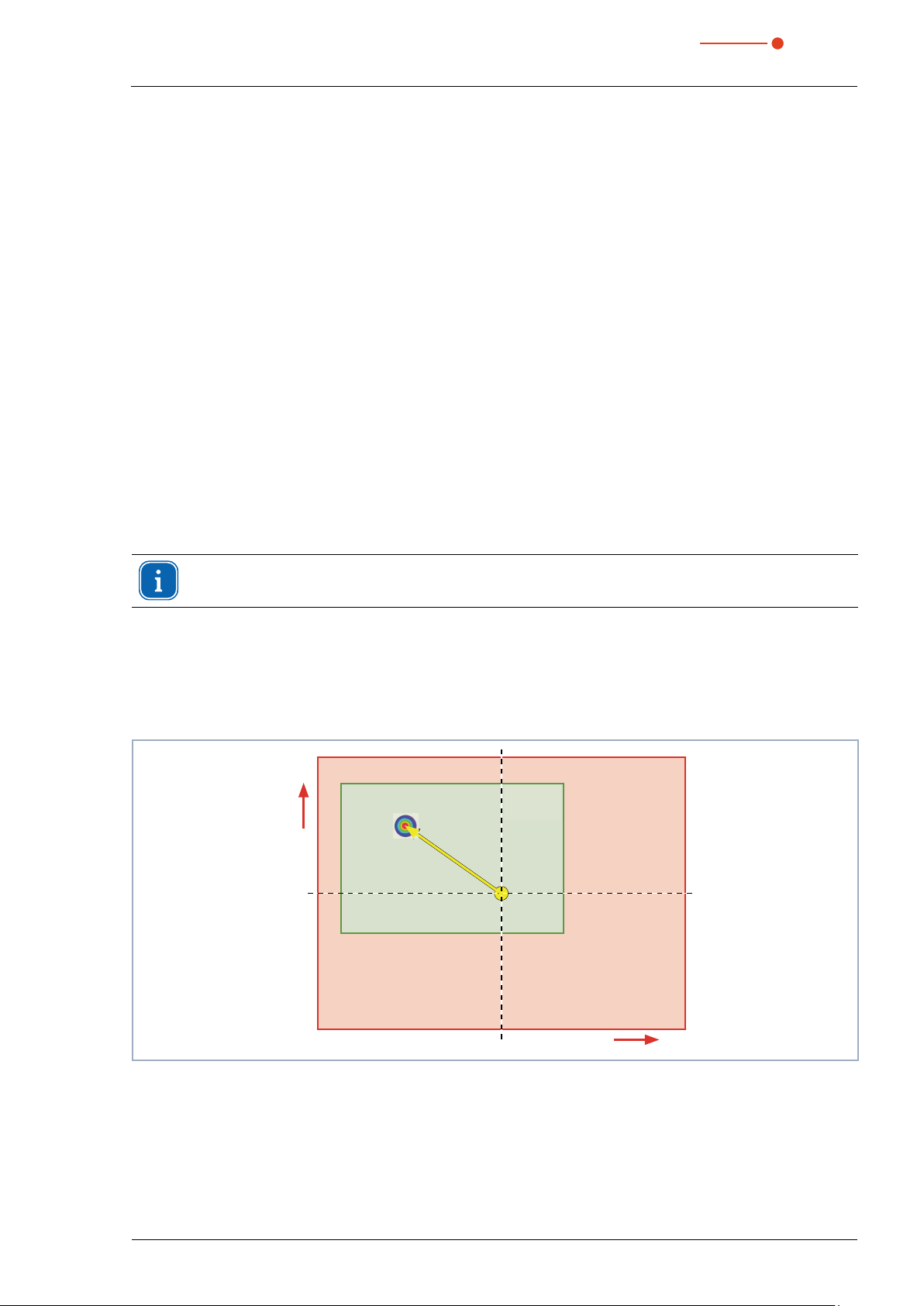
Fig. 12.7: Coordinates of the pkl-export function (the illustration is not to scale)
Revision 01/2019 EN
x
41

MicroSpotMonitor MSM
35,0(6
12.2.7 Load measurement preferences (menu File > Load measurement preferences)
Stored settings can be resorted to with Load measurement preferences. The standardized extension for a
setting file of the MicroSpotMonitor MSM is “.ptx”.
12.2.8 Save measurement preferences (menu File > Save measurement preferences)
The current measurement settings are stored (.ptx-file).
12.2.9 Protocol (menu File > Protocol)
The calculated measurement results from a single plane can directly be written into a text file.
The following is stored:
• Date and time of the measurement
• Beam position and beam radius (according to 86%- and 2. moment method definition)
Therefore please activate the check box Write. Then you can directly enter the name in the field Filename or
you can use the standard selection menu with the button Browse.
Fig. 12.8: Window Protocol
12.2.10 Print (menu File > Print)
You can print directly from the program. The current window can be printed with the menu point Print in the
menu File. With the menu point Settings it is also possible to change the settings as far as the formats etc.
are concerned.
12.2.11 Print preview (menu File > Print preview)
Shows a preview of your printing order.
12.2.12 Recently opened files (menu File > Recently opened Files)
Selection of the files processed before.
12.2.13 Exit (menu File > Exit)
Terminates the program.
42
Revision 01/2019 EN

MicroSpotMonitor MSM
35,0(6
12.3 Edit
12.3.1 Copy (menu Edit > Copy)
By means of the copy function a direct export of graphics to other programs is possible. In this case the
content of the current window is transmitted to the Windows clipboard.
12.3.2 Clear plane (menu Edit > Clear plane)
The content of the actual displayed measurement plane of the measurement data set selected in the toolbar
is deleted.
12.3.3 Clear all planes (menu Edit > Clear all planes)
The content of all measurement planes of the measurement data set selected in the toolbar is deleted.
12.3.4 Change user level (menu Edit > Change User Level)
By entering a password a different user level can be activated.
Revision 01/2019 EN
43

35,0(6
12.4 Measurement
12.4.1 Measuring environment (menu Measurement > Environment)
MicroSpotMonitor MSM
Fig. 12.9: Dialogue window Measuring Environment
In the dialogue window Measuring Environment data such as the laser type, focal length etc. can be
stored. These data can be read via Presentation > Review.
Focal length
Stating the focal length is relevant for the evaluation of the caustic measurements. From the caustic process
and the entered focal length the raw beam diameter on the focussing optic can be calculated.
Wave length
The wave-length is the basis for a correct determination of the beam quality factor M². There are the following options:
• 1.064 μm for Nd:YAG laser
• 0.532 μm for Green laser
• 0.355 μm for UV laser
A wavelength can also be typed in numerically.
While only the calibration points of the measuring objective can be configured in the CCD Settingdialog window, the exact value of the laser’s wavelength can be entered in this window. This value is used in all numeric
evaluations, such as the calculation of the beam quality factor M².
Caution: If the wavelength is newly selected in the CCD Setting dialog window, the value in this
window will be overwritten with the selected calibration point.
44
Revision 01/2019 EN

MicroSpotMonitor MSM
35,0(6
Application
By means of the button Apply the entries can also be changed after a measurement. With the button
Apply all planes the entered values are inserted and settled, while the button Apply only refers to the value
in the current plane.
Laser power
Entering the laser power is a reference value for the relative power position in the menu point Single measurement or Caustic measurement. Furthermore, a z-axes offset as well as a coordinate rotation angle can
be entered.
Comment
Please do not use the character # in the comment field “Comment”. This character is used as a separator
in the software. If it is entered in the field “Comment”, problems could occur when it comes to storing or
activating measuring data.
A line break can be enforced by means of the key combination: <Ctrl> + <Enter>.
12.4.2 Sensor parameters (menu Measurement > Sensor parameter)
Adaptable squares
Z
Y
Fig. 12.10: Dialogue window Sensor parameters
Mechanical limits
By pulling the turquoise square with the mouse pointer you can restrict the movement range of the y- and zaxis. Therewith you can prevent damages in case other components reach into the movement range of your
device. The maximum value corresponds to the value Y3 and Z3.
Device
By means of this option, you can select the device which is supposed to be operated. Depending on the
number of devices connected, additional device numbers are assigned.
RPM
Not relevant for MicrosSpotMonitor MSM.
Revision 01/2019 EN
45

MicroSpotMonitor MSM
35,0(6
Resolution
Here you can enter the number of pixels in the measuring window, ranging from 32 x 32 to 256 x 256 pixels.
Generally, 64 pixels per line and a total of 64 lines is sufficient. Please keep in mind that the more pixels there
are, the longer the measurement will take.
Detector
Not relevant for MicrosSpotMonitor MSM.
Manual z-axis
With this function you can deactivate the z-axes of the measuring system. This is useful if you want to use
external movement axes. In this case you can manually assign a z-value to every measurement plane in the
dialogue window Single measurement.
12.4.3 Beam find settings (menu Measurement > BeamFind Settings: Beamfind
Not relevant for MicrosSpotMonitor MSM.
46
Revision 01/2019 EN

MicroSpotMonitor MSM
35,0(6
12.4.4 CCD info (menu Measurement > CCD Info)
The most important device data is shown in the menu Measurement > CCD Device Info. Here you can see
the magnification information for the measuring objective and also check which beam path is turned on.
If obvious default values (1:1) are shown instead of the actual magnification, then please check the mounting
of the measurement objective.
Fig. 12.11: Window CCD Info
Revision 01/2019 EN
47
35,0(6
12.4.5 CCD settings (menu Measurement > CCD Settings)
MicroSpotMonitor MSM
Fig. 12.12: Dialogue window CCD Settings
The wavelength, attenuation, and operating mode are all set in the CCD Settings dialog window.
Trigger modes
The appropriate settings must be configured here in keeping with the operating mode of the laser to be measured. Here it is important to consider that pulsed lasers with a pulse frequency of more than 500 Hz can be
measured in cw mode. If, however, the operating mode is set to pulsed and a cw laser system is involved,
the measuring device will always display the error message “Error Black Pixel Measurement” or “Time Out
During Measurement” in reaction to a measurement request.
Delay
This function can only be used with a “triggered operation” trigger mode. The time the measuring system
should wait between when it detects the trigger pulse and the start of the measurement is set here. Together
with the function “Integration Duration”, defined “Windows” from the plus cycles can be measured (e.g. exactly one pulse or parts of an ms pulse. The minimum delay is 12µs.
CCD operating modes
Three different modes can be set here. If the Raw Data setting is activated, the measuring system will return
the uncompensated data of the CCD when a measurement is requested. Especially with NIR irradiation,
these can be riddled with measuring errors such as “smear effect” readout noise. Even the numeric beam
data generated generated from this data will be affected by this.
If a Background is selected as the operating mode, only correction data will be returned while measuring.
Measuring Data mode should always be the default setting here though. Only when this mode is turned on
can the measuring system deliver reliable measuring values.
48
Revision 01/2019 EN

MicroSpotMonitor MSM
35,0(6
Integration duration
This function sets a defined integration duration. The optimizer must be deactivated before this can be accomplished, since otherwise the measuring device itself will optimize and thus change the integration duration. This function is also used mainly in measuring pulsed laser systems.
Filter wheel
Which filter is needed for measuring depends on the wavelength and the intensity of the laser beam being
measured and the appropriate one must be chosen specifically for each measuring task.
A filter can be considered suitable when all measuring planes of a caustic measurement can be measured
using an exposure time between 18ms (-20dB) and 0.18ms (-60dB). Outside of these limits, the S/N ratio
of the CCD declines, thus reducing the accuracy.
Wavelength
Due to the wavelength-dependent overall magnification of the camera-based measuring system, it is important to check that the right selections have been made before each measurement. The wavelengths shown
here represent the calibration points of the measuring objective. As a result of the achromatic properties of
the measuring objective, a wavelength range between 1030 and 1100 can be achieved, for example, with a
calibration point at 1064 nm without causing generating measuring errors.
Trigger
The trigger menu is only pertinent when measuring pulsed laser systems. A fixed value (2001) is generally
specified for the trigger diode by default. This value describes the threshold value at which a trigger signal
is emitted. If you switch the trigger to automatic, the trigger level will first be set to the maximum value. The
Test button is renamed in Optimize. In the optimize routine (laser must be turned on), the trigger threshold
is lowered gradually until the MicroSpotMonitor starts receiving trigger signals (lower trigger level). The trigger
level is then increased until the MicroSpotMonitor stops receiving trigger signals (top trigger level). The final
trigger level is determined by calculating the arithmetic mean of the two limit values. External trigger entry
can be activated via the menu point Trigger Channel. Transfer signal pertains to the transfer output of the
MicroSpotMonitor. Here it is possible to define the CCD sensor state at which there should be a trigger signal
(e.g. for turning on the laser).
Fig. 12.13: Trigger connections
Revision 01/2019 EN
Input
external trigger
BNC
Ausgang
Interer Trigger
BNC
49
35,0(6
12.4.6 LQM adjustment (menu Measurement > LQM Adjustment)
Not relevant for MicrosSpotMonitor MSM.
12.4.7 Power measurement (menu Measurement > Power Measurement)
Not relevant for MicrosSpotMonitor MSM.
12.4.8 Single (menu Measurement > Single)
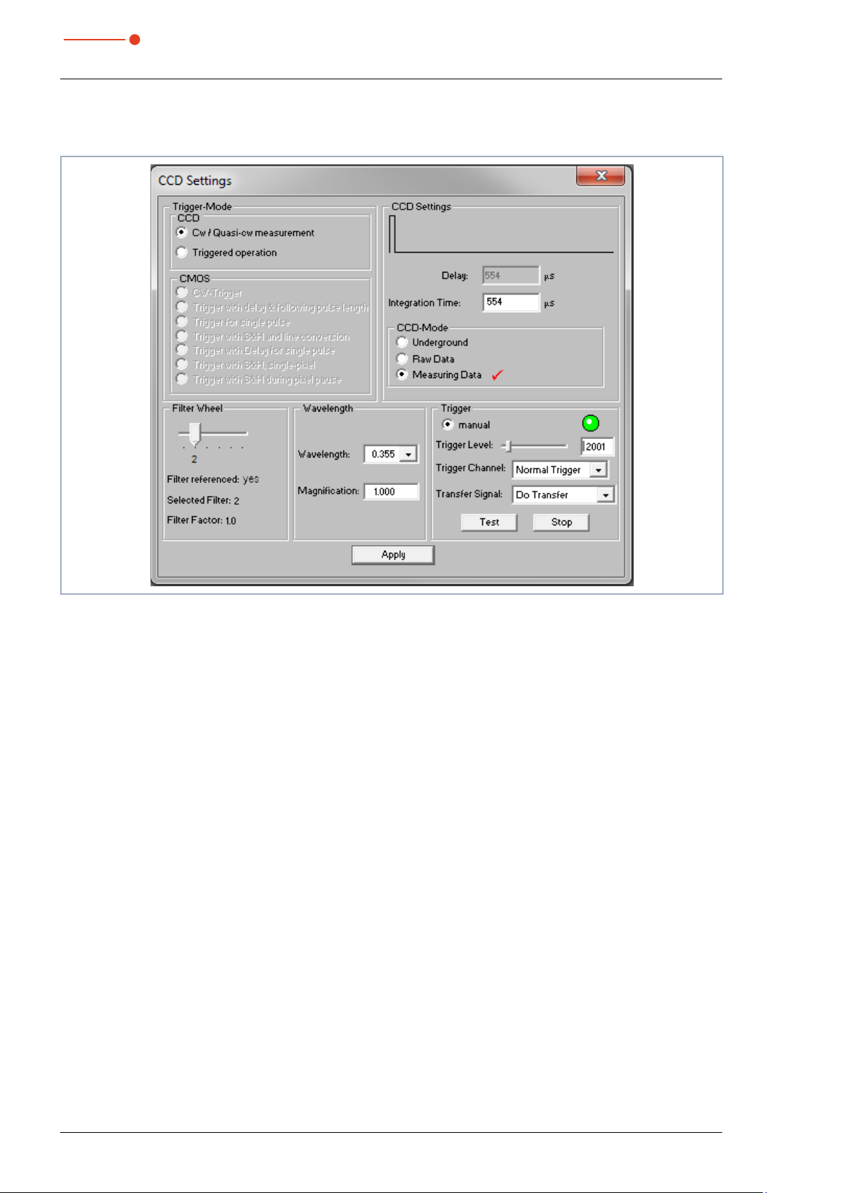
23
22
MicroSpotMonitor MSM
1
2
3
4
5
21
20
Fig. 12.14: Dialogue window Measurement settings
6
7
8
9
10
11
12
13
141516171819
50
Revision 01/2019 EN

MicroSpotMonitor MSM
35,0(6
1 Single
Monitor
Video Mode
2 Start Starts a measurement in the currently chosen plane
3 Stop Finishes the measurement in the currently chosen plane
4 Reset The measuring device is reset
5 Stop Motor Not relevant for MicrosSpotMonitor MSM
6 Plane Selection of the measuring plane (0-49) either explicit or by means of the buttons (+/-)
7 Entry field Numerical entry of the z-position
8 Copy Copies all settings (window size and window position; x, y, z; etc.) from the former plane
9 Find beam Starts an automatic beam search in the current measuring plane
10 Scan Starts an automatic beam search with the MicrosSpotMonitor MSM. The algorithm
11 Ampl. Slide control in order to adjust the optical amplification (exposure time of the CCD)
12 Power Slide control in order to adjust the laser power to save it in the software
13 Entry field Power Numerical input of the laser power to save it in the software
14 Entry field Ampl. Numerical input of the electrical amplification
Starts a measurement in the chosen plane
Starts repeated measurements in the chosen plane automatically
to the current plane (e.g. 1>>2)
works at a fixed z-position and searches only within the range of the specified measuring
window.
15 Averaging Analysis of the serial measurements. Averaging algorithms: average value, values of the
16 Averaging Selectable number (1 – 50) of single measurements for the averaging
17 LED symbol and
bar graph display
18 False color Activates the option of the false color presentation
19 Zoom Magnification settings for the measuring window
20 Symmetric This option enforces the usage of square measurement windows, whose size is only
21 X/Y Set the measurement window size for non-square windows
22 Display Measuring window shows the current measuring result
23 Z Slide control in order to set the z-position
Tab. 12.2: Explanation of input and setting elements
maximum pixels and the value of the maximum trace
Display for the degree of the signal saturation (LED green ≙ ok, red ≙ not ok)
adjustable via x.
Revision 01/2019 EN
51

MicroSpotMonitor MSM
35,0(6
With the dialogue window Measurement settings either single measurements or repeated measurements
can be carried out. The measuring window position can be set either manually or automatically.
Controlling measuring modes (individual measurement, monitor, and video mode)
There is a total of three different measuring modes that can be selected here. In the Individual Measurement and Monitor measuring mode, all necessary compensations (smear effect, diffusion) and exposure
time adjustments are performed every time a new measurement is carried out. Valid measuring data is generated in this mode.
The measuring mode VideoMode does not produce valid measurement data. Here the exposure time is
carried over from the last measurement and does not vary. Compensation measurements are not performed,
making it unnecessary to consider or compensate for measuring artifacts such as smear effects.
Due to the “high” measuring frequency of about 5 Hz, this operating mode is particularly suited for use when
aligning the device. The numeric results should not be interpreted absolutely, but rather always relative to
each other.
Power
The slider sets the actual laser power, so the software algorithm can calculate the spacial power density. It
can be set to any power up to the maximum.
The maximum power is entered in the menu under Measurement > Environment. The power density is
calculated in relation to the power values set here. Up to 50 individual measurements can be recorded in a
measurement file. The results can be easily compared and analyzed with the various presentation functions
of the LaserDiagnosticsSoftware LDS.
Optical amplification (opt. ampl.)
This function activates the automatic adjustment of the exposure time of the CCD for every measurement.
The function must be activated in order to keep the signal/noise ratio consistently high for a caustic measurement.
For special measuring applications, however, it might make sense to deactivate this function and set the exposure time to a fixed value between 12 µs and 200 ms. Here it is important to ensure sufficient attenuation
of the laser beam with the help of the fixed ND filter or the filter wheel.
Copy
Using the Copy button, you can apply the measurement settings for window size, window position, power,
and amplification from the previous measuring plane.
Beam search
The Beam Search will initiate an automatic beam search. When this happens, the system will only search
the area of the currently set window for the set z position.
If the beam search is completed successfully, a measuring window with the appropriate size and position
will appear on the display screen. The beam can then be accepted using the Start button. The size of the
measuring window depends on the magnification of the measuring objective. The measuring objective and
the wavelength are the influencing variables here.
Scan
For devices such as the LaserQualityMonitor LQM, the measuring window is much smaller than the measuring area defined with the x- and y-axis (2 mm x 2 mm). The beam search is therefore supplemented with the
Scan command. Once a scan is initiated, the MicroSpotMonitor MSM will automatically sense the measuring
area. If a point of maximum intensity can be identified, the MicroSpotMonitor MSM will automatically zoom in
on this area and adjust the measuring window size accordingly.
Size of the measuring window
During a manual beam search, you can define the location and size of the measuring window yourself in
the dropdown menu within the mechanical limits. You can change the location of the measuring window by
clicking on it and dragging the frame with the mouse.
52
Revision 01/2019 EN

MicroSpotMonitor MSM
35,0(6
Z-Slider
The location of the window in the z direction (height) can be set by the z-slider or entering a numeric value.
Symmetrical
Once this function is activated, only rectangular measuring windows will be allowed. In cases where an elliptical or even a square laser beam is being measured, this function should be deactivated so that the measuring window can be optimally adjusted.
False color rendering
False color rendering is activated by clicking on the corresponding button. A measurement is initiated by
clicking on the Start button. Selecting Monitor and pressing the Start button will initiate an ongoing, repeating measurement with the current settings. The repeat rate depends on the spacial resolution and the type of
communication between the PC and the MicroSpotMonitor MSM.
Zoom function
The zoom function allows for detailed magnification of the measuring area.
Revision 01/2019 EN
53

MicroSpotMonitor MSM
35,0(6
12.4.9 Caustic measurement (menu Measurement > Caustic)
The caustic measurement is a serial measurement where the z position is varied. The results are stored in
different planes. A different z-position is assigned to every measuring plane. As the beam radius as well as
the power density change in every z position, the position as well as the size of the window and the signal
strength can vary from plane to plane. The parameters are automatically adjusted in the process and can
also be configured separately for each measuring plane.
Parameters (start number of the plane)
Under Start, the start number at which the measurement is initiated can be entered for the plane. By default,
the start number is generally set to zero and should only be changed when you are measuring in an existing
document and don’t want the existing measurement data to be overwritten. If, for example, you have measured a caustic with 21 planes and want to magnify the measuring area to the smaller z-values, you can set
the start plane to 21 and modify the measuring area appropriately. The new measuring values will then be
written into the existing document starting with plane 21.
In the Quantity selection field, the number of planes to be measured in the specified z range is set. The following should be considered here:
• Since the LaserDiagnosticsSoftware LDS always sets the measuring plane distances so they are equi-
distant (equal spacing) and the measuring area is almost always situated symmetrically around the focal
point, an odd number of measuring planes should be selected. This ensures that the focus plane is
measured.
• Beam measurement norm DIN 11146 specifies that at least 10 measuring planes should be measured.
Furthermore, five measurements should also be taken within a Rayleigh length and the other beyond 5
Rayleigh lengths. In order to meet all of the requirements with equidistant distribution, at least 17 measuring planes must be measured in a range of ± 3 Rayleigh lengths.
Mode (automatic and manual settings)
There are two different measuring modes for caustic measurement. In “Automatic” mode, the measuring
system and the LDS determine the ideal measuring window position (x- and y-direction) for each measuring
plane and the optimal measuring window size for the fill factor. Furthermore, the plane location in the z-direction is also calculated based on the specifications (number of measuring planes, measuring limits z-direction).
Especially when adjusting the measuring window size and the measuring window position in the xand y-direction, the number of iterations (max. three per plane) can result in an extended measurement duration.
It is therefore possible to change the measuring mode to “Manual Settings” for recurring measuring tasks
and for repeating measurements. In this case, the measuring system will take the measuring window positions and measuring window sizes from the previous measurement or from a .ptx file. This reduces the measurement duration considerably, but does require that the location and parameters of the laser beam change
only minimally.
Beam search
This selection field specifies which plane the caustic measurement should be started in. If the optional Beam
Find function is activated in the Options dialog window, that is also the plane in which this function will be
performed. When the Beam Find function is deactivated, this plane must be manually measured ahead of
time to make sure that the laser beam is found.
The window can be adjusted under the Adjust menu point. The settings for spacial resolution of the beam
search, the threshold value, and the minimum signal strength can be entered under the Details menu point.
Beam search can be turned off in the Measurement > Option (only for advanced users) menu by deactivating the checkbox Enable Beam Find Process.
54
Revision 01/2019 EN

MicroSpotMonitor MSM
35,0(6
Automatic caustic measurement (menu Measurement > Caustic > Automatic)
Fig. 12.15: Dialogue window Caustic settings
During automatic caustic measurement, the minimum and maximum z-position is selected together with the
number of measuring planes. The measurement cycle begins with an automatic beam search in the specified
starting plane. The beam search only occurs within the area of the starting plane’s measurement window.
Settings can be entered manually. After manually entering the settings for the measurement planes as described in the following section, the caustic measurement can be repeated automatically by choosing the
Manually adjusted mode.
It is also possible to store measurement settings such as window size, position, etc. in a data file to be reloaded again if necessary (File > Safe/Load measurement preferences).
A measurement cycle is started by pressing the Measure button. All planes will be measured then one after
the other during the measurement cycle.
Manual caustic measurement as time series (menu Measurement > Caustic > Manually adjusted)
The manual caustic measurement consists of a series of individual measurements at various z-positions, with
the results being stored in their own planes.
12.4.10 Start adjust mode (menu Measurement > Start Adjust mode)
Not relevant for MicrosSpotMonitor MSM.
Revision 01/2019 EN
55

35,0(6
12.4.11 Option (advanced user only) (menu Measurement > Option)
MicroSpotMonitor MSM
Fig. 12.16: Dialog window Option
Enable beam find process
The Beam Find function must be used for caustic measurement. This involves an algorithm that separates
the measuring signal from the measurement artifacts (e.g. noise) via an adjustable trigger threshold and
adapts the size of the measuring window to this signal. This algorithm is only executed in the beam search
plane (Dialog window Caustic). On all other measuring planes, the measuring window size is determined using the fill factor.
If this function is deactivated, the beam search plane must be manually “premeasured” in the measuring
system. Otherwise the measuring system might end up positioning the measuring window on the edge of the
measuring area where there is no measuring signal. This makes it impossible to take a meaningful measurement.
If you turn the Beam Find function off and have the measuring measure the beam search plane system before each caustic measurement, you can save about 20 sec of measuring time per caustic measurement.
Summary: This function should be activated by default and only deactivated by experienced users. Turning
off this function can shorten the time for caustic measurements by about 15%.
Fillfactor
The fill factor is the quotient of the beam diameter and the length of the sides of the measuring window. As
long as the measuring signal is not cut off and there are no noise components in the measuring result and
now errors in the offset determination, the fill factor won’t influence the accuracy at all. But since every real
measuring signal is tainted with noise and since the precision with which the zero level of a measuring signal
can be determined is finite, very small fill factors can lead to a high level of accuracy. Depending on how
substantial the RMS noise is and the errors in the zero level determination of a measuring plane, the optimal
fill factor value to produce the best possible mathematical result will be different.
56
Revision 01/2019 EN

MicroSpotMonitor MSM
35,0(6
For TopHat and Gaussian beam shaped laser beams, the fill factor should range between 0.5 and 0.7. If the
beam has diffraction rings, however, and if these are located completely within the measuring window, the
optimal value for the fill factor can be between 0.5 and 0.6.
By default, the value should be set to: “Max 0.7 Min 0.5 Target 0.6”. For extremely deformed beams, the
value may be changed to “Max 0.6 Min 0.4 Target 0.5”.
Font size
The font size for the most important display window can be changed here.
It is set to 10 points at the factory.
Open windows
When the window opening function is activated, some basic windows are opened when the LDS is started. If
you don’t want this to happen, the function can be deactivated.
Revision 01/2019 EN
57

MicroSpotMonitor MSM
35,0(6
12.5 Presentation
This chapter describes the presentation, analysis and storage of measuring results.
In order to carry out comparisons between different measurements, the program can manage several
measuring data sets simultaneously. The opened data sets are shown in the toolbar. In order to open one
presentation, the data which is to be examined is selected in the list of the data selection and afterwards the
desired kind of presentation is chosen.
File management functions as well as various display types can be pulled up directly with the symbols in the
menu bar.
Fig. 12.17: Selection of a data set
On the selection plane, it is possible to switch back and forth between different image storages of the measuring series. When plane selection is activated, it is possible to move up or down by clicking the cursor.
When plane selection is set to Global in the display menu, then it is also possible to move up/down with the
cursor button.
In the menus for the notation of single measurements (Presentation > Variable contour lines, Presentation
> Isometry and Presentation > False color presentation) the option Autoscale effects the usage of the
entire display range for the measuring values.
Moreover, you have the possibility of switching between different image memories of series of measurements
by means of the Plane selection. Switching is also possible by means of the cursor keys up/down if the
plane selection is selected. If the plane selection in the display menus is set on Global, switching simultaneously between the planes is possible via the selection in the toolbar.
The title of the dialogue window indicates the name of the data sets shown.
For the parallel evaluation of several measurements the program has 50 image memories which can record
one measurement each. These image memories (measuring plane) can also be used in order to record
changed measurement values in case of a parameter variation.
Due to the variation of the z-position in the different planes a caustic measurement is realized. Due to a
change of the laser power it is possible to simulate, e.g. the thermal inflow-behavior of the system. Similarly,
time series are possible. Respective displays are, for instance, possible by means of the menu item Presen-
tation > Graphical review.
58
Revision 01/2019 EN
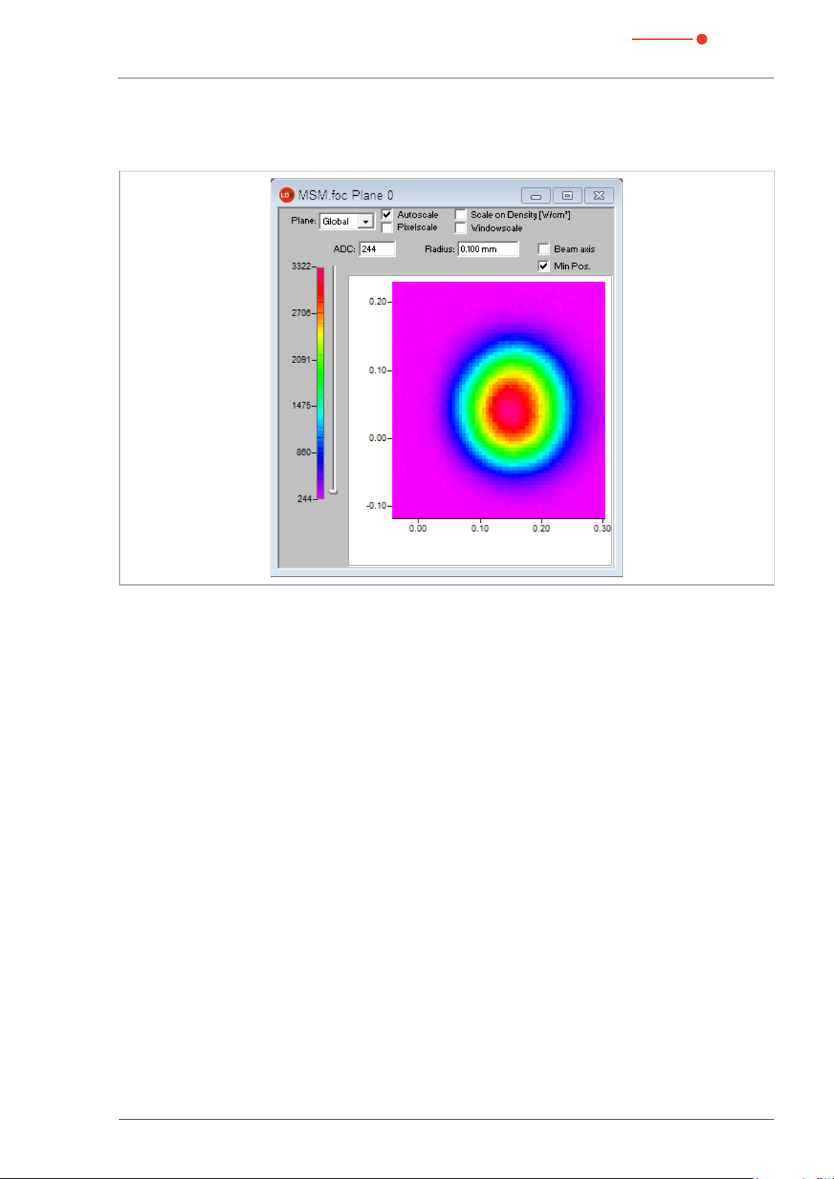
MicroSpotMonitor MSM
35,0(6
12.5.1 False colors (menu Presentation > False colors)
Here, a false color presentation of the measured power density distribution is generated.
Fig. 12.18: Dialogue window False colors
The used color scale is shown on the left. For a higher sensitivity, e.g. for the analysis of diffraction figures, it
is possible to switch the used color scale in the menu Presentation > Color Tables. By means of the slide
control on the left hand side of the color scale you can display the sections of different ADC values with the
corresponding radii.
Apart from the automatic scaling, there are three more types of scaling:
Scale on density
All planes of a caustic measurement are scaled on the maximum measured power density. This is supposed
to help comparing the different planes more easily.
Pixel scale
This scaling is only interesting when it comes to the usage of asymmetric measuring windows. In this case
the axis of the windows are no longer a function of the measuring window size but of the number of pixels
measured.
Window scale
With regard to this function, all measuring windows of a caustic measurement are enlarged to the size of
the maximum measuring window. This function, too, is supposed to help comparing the different measuring
planes of a caustic measurement more easily.
The beam axes can be displayed in all types of scaling by activatng the check box Beam axis.
Rule function
The beam can be measured in any direction by left-clicking on the image.
Revision 01/2019 EN
59

MicroSpotMonitor MSM
35,0(6
12.5.2 False colors (filtered) (menu Presentation > False colors (filtered))
The special function of the filter is called spline – function. It is characterized by the fact that the position of
the maximum is maintained. The single pixels in the matrix are weighed by means of a 1-2-1 filter in order to
reduce the noise.
This filter can also be used multiple times without the position of the maxima being moved.
Fig. 12.19: Dialogue window False colors (filtered)
12.5.3 Isometry (menu Presentation > Isometry)
This menu item generates a spatial display of the measured power density distribution of a plane. The false
color display can be deactivated. A turn of the distribution by 90°, 180° and 270° each is possible.
Fig. 12.20: Dialogue window Isometry (on the left with a deactivated color display)
60
Revision 01/2019 EN

MicroSpotMonitor MSM
35,0(6
12.5.4 Isometry 3D (menu Presentation > Isometry 3D)
This function generates three-dimensional displays of the power density distribution of a plane and all planes
in false colors.
The presentation window is divided. On the left the caustic, on the right the power density distribution in a
plane is displayed. The horizontal size of the single windows can be changed by drawing the separating bar
by means of your mouse.
The graphics can be rotated along all three axis with the left mouse button and with the right mouse button
they can be positioned in the window.
1 2 3 4 5 6 7
Change window size
Fig. 12.21: Dialogue window Isometry 3D
1 3D presentation of the
plane
2 3D presentation of the
caustic
3 Magnification in the plane In the left part of the presentation window a magnification of the plane displayed
4 Rotation Causes a rotation of both graphics along the z-axis.
5 Plane selection Here the plane, which is to be displayed, can be chosen (you can also choose
6 Zoom Slide control for a continuous magnification of the presentation
7 Contour Slide control for a contour trimming along the power density.
Tab. 12.3: Explanation of selection and setting elements
Inserts the 3D presentation of the power density distribution in the plane in the
display window.
Additionally inserts the 3D presentation of the caustic in the presentation window.
on the right is inserted (the desired area can be clicked by means of the left
mouse button in the right window).
the desired plane in the 3D caustic by means of the left mouse button).
Revision 01/2019 EN
61

MicroSpotMonitor MSM
35,0(6
12.5.5 Review 86% or 2. moment (menu Presentation > Review (86%)/(2. moment))
For the radius definition there are two basic determination possibilities:
• Determination of the beam radii according to the 86% - power definition,
(see chapter 22.2.4 on page 145).
• Determination of the beam radii according to the 2. moment method (ISO 11146),
(see chapter 22.2.3 on page144).
Tab. 12.4: Result window 86% Review
Tab. 12.5: Result window 2. Moment Review
The parameters and results of the current selected plane are highlighted in blue. When the measuring signal
only exceeds the zero level by a little bit, the measuring results are not shown in black, but rather in gray. In
this case, check to see if the measuring values are reliable or need to be thrown out and the measurement
repeated with different settings.
The entries for power, focal length, and wavelength as well as any comments can also be changed after the
fact. For this purpose there is the button Apply in the menu item Measurement > Environment.
62
Revision 01/2019 EN

MicroSpotMonitor MSM
35,0(6
12.5.6 Caustic (menu Presentation > Caustic)
The results of the caustic measurement can be displayed by means of the menu item Presentation >
Caustic. On the left Fig. 12.22 on page 63 shows the measured beam parameter either on the basis of
the 86%-radii or the 2. moment method evaluation according to ISO 11146. In the middle of the picture the
graphic shows the caustic profile. The beam radii are depicted on the beam spread direction. On the right is
a false color presentation of the measurement plane selected with the mouse shown together with numerical
results of this corresponding plane.
Fig. 12.22: Dialogue window Caustic
The red line depicts a compensation curve according to the calculated fits which can be displayed via the
check box Fit in the 2D presentation.
Compensating curve
In order to evaluate the caustic, a hyperbolic compensating curve (ISO 11146) is adapted to the measuring values. This compensating curve describes the propagation of an ideal laser beam mathematically. The
development of the compensating curve is theoretically determined by means of the following parameters:
• Standardized beam quality factor M² or respectively beam propagation ratio K
• z-position
• focus radius
• rayleigh length
Standardized beam quality factor M² (or respectively the beam propagation ratio K=
The normed beam quality factor describes how well the affected laser beam can be focused in relation to the
dominant mode. The basic mode represents the theoretically best possible beam and has a beam quality
factor M² of 1. All other beams have higher M² values.
)
Revision 01/2019 EN
63

MicroSpotMonitor MSM
35,0(6
Z-position
This value provides the position of the focus points in the z-position. As the compensation curve takes the
measurement points into consideration, the calculated z-position is not necessarily located at the position,
which has measured the smallest radius.
Focus radius
The focus radius is the smallest beam radius in the caustic. Generally, this value is similar to the smallest
value measured, but not necessarily.
Due to different reasons it may occur that the adaption to the measurement values was not carried out. This
is the case if the compensation curve does not lie close to the measurement values. In this case the parameters of the adapted compensation curve are to be discarded.
Rayleigh length
The Rayleigh length is a derived parameter and describes the distance in z-direction with regard to which the
beam radius has increased by the factor √2 (=1.41) and concerning which the beam area has increased by
the factor 2. The Rayleigh length increases with the focal length of the focusing optics and the beam quality.
The doubled Rayleigh length is an approximate point of reference, up to which material thickness (metal) a
procession is possible with the optic employed.
In order to make sure that the adapted values have a high significance, the measurement is to be carried out
in a z-range of at least ±2 Rayleigh-lengths. As demanded in the ISO 11146 5 to 6 Rayleigh-lengths would
be ideal. However, this demand is often confronted with the problem of quickly sinking power densities of the
laser beam which is to be measured. In case of a distance of 2 Rayleigh-lengths from the focus the power
density has sunk to just a quarter.
In this case the caustic measurement consists of a compromise between the desired measurement range in
z-direction and the power density (signal-to-noise ratio) necessary for a perfect measurement.
Cyclic caustic measurements
When performing cyclic caustic measurements, it is useful to store settings for various display parameters in
a data file. This data is available anytime and can be reloaded for a new measurement. For a quick check of
the beam or when it is necessary to measure only part of the caustic.
Cyclic measurements are normally performed over a period of 2 to 3 minutes; by Ethernet communication
much quicker. For measurements after laser or system servicing, you should use more planes to achieve
greater accuracy in the results.
To start a measurement, saved caustic data is loaded from the settings file. This is done through the menu
item File > Load Settings. The data is loaded after entering the desired file name.
64
Revision 01/2019 EN

MicroSpotMonitor MSM
35,0(6
Advanced (menu Presentation > Caustic > Advanced)
Fig. 12.23: Result window Results X,Y (2. moment)
For the examination of asymmetric beams the dimensions of the main axes of the beam can be determined.
On the basis of these values the program also calculates direction dependent beam propagation factors as
well as beam position values. The related curves are shown via the two check boxes radius x, y while the
numerical values are provided by the result window.
Raw beam (menu Presentation > Caustic > Raw Beam)
Not relevant for MicrosSpotMonitor MSM.
Revision 01/2019 EN
65
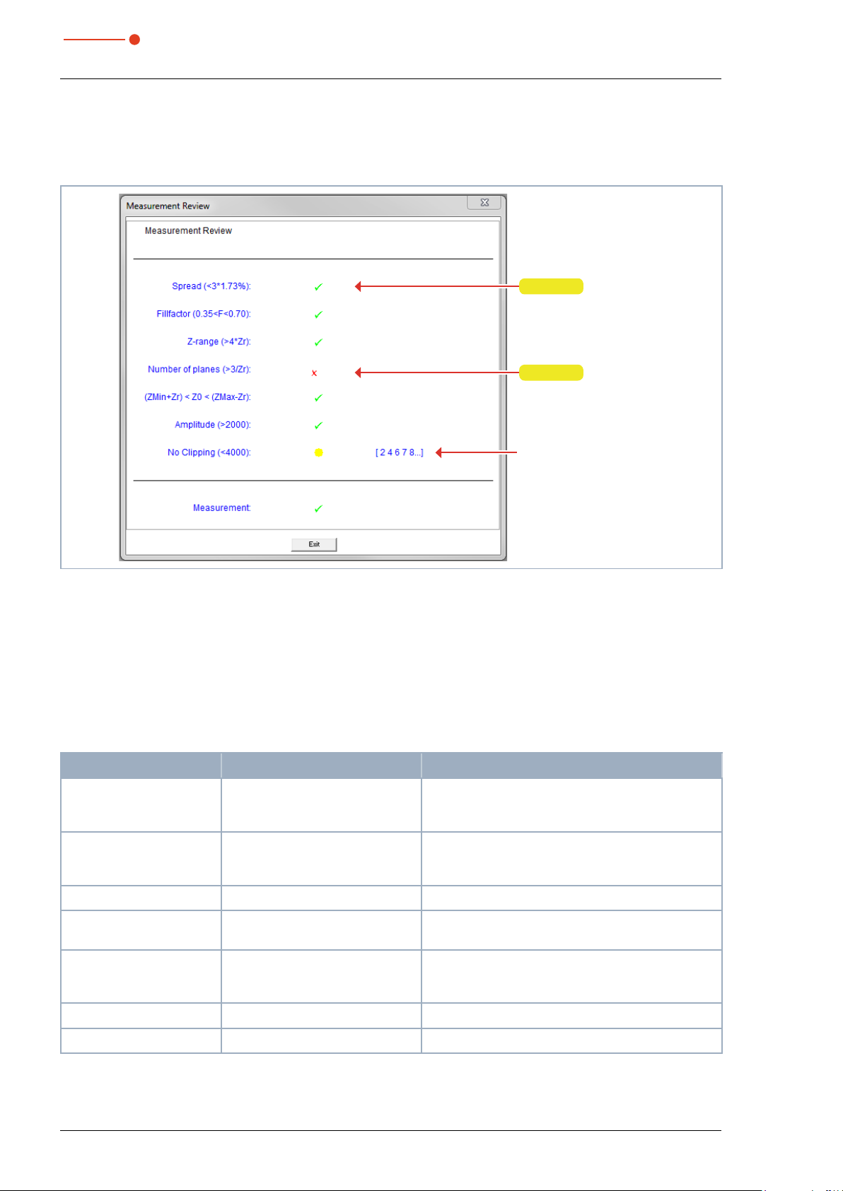
MicroSpotMonitor MSM
35,0(6
Review (menu Presentation > Caustic > Review)
This function checks whether the results and settings of the caustic measurement are within the reliable
range.
OK
Not ok
Borderline results
(in the measuring planes
2, 4, 6, 7 and 8)
Fig. 12.24: Result window Measurement Review
Under “spread” the average standard deviation of the caustic fit according to the 2. moment method radii is
stated. A “tick” () is set if the standard deviation is smaller than 3.5% and if all of the measuring values lie
within a range of ±3%standard deviation.
When the divergence receives a negative assessment (û) the affected measuring planes are also displayed.
The displayed planes are arranged from left to right, starting with the greatest divergence and working its
way down. This means that the plane with the greatest divergence (see Fig. 12.24 on page 66 Plane 2) will
be the first one in front.
Valued functions Test criterion
Spread Average relative standard devia-
Fill factor Describes the ratio of the beam
Z-range Measuring range in z-direction At least 4 Rayleigh-lengths
Measurement planes Number of measurement planes
) < Z0 < (Z
(Z
Min+Zr
Max−Zr
tion of the caustic fit according to
the 2. moment method
diameter to the lengths of the
sides of the measuring window
per Rayleigh length
) Minimum measurement range
above and below the focusing
plane
Positive evaluation
Standard deviation < 3.5%, all measurement values
within a range of ± 3 % standard deviation
In the range 0.35 – 0.7
At least 3 measurement planes per Rayleigh length
The focus lies within the minimum measurement
range and this range accounts for at least one Rayleigh length in every z-direction
Amplitude (>2 000) Signal control Above 2 000 counts
No Clipping (<4 000) Signal control Below 4 000 counts
Tab. 12.6: Criteria for the evaluation
66
Revision 01/2019 EN

MicroSpotMonitor MSM
35,0(6
If all criteria are fulfilled, the measuring results have a high reliability. The absolute accuracy can not be stated
from the standard deviation from the fits as all the systematic measuring errors as well as the accuracy of the
calibration are additionally taken into account when it comes to the absolute error.
12.5.7 Raw beam (menu Presentation > Raw-beam)
Not relevant for MicrosSpotMonitor MSM.
Revision 01/2019 EN
67

MicroSpotMonitor MSM
35,0(6
12.5.8 Symmetry check (menu Presentation > SymmetryCheck)
This display menu checks the rotational symmetry of the power density distribution of a laser beam. It can,
for instance in connection with the monitoring operation (Measurement > Single > Monitor), be used for
the alignment of laser resonators.
In the following, the figures Fig. 12.25 on page 68 and Fig. 12.26 on page 68 show two examples for
the possible results of a symmetry check at an elliptic beam and a circular beam.
Fig. 12.25: Dialogue window (menu Presentation > Isometry) power density distribution of an elliptic beam
The power density distribution of an elliptical beam as shown in Fig. 12.26 on page 68 together with the
Symmetry check comes to the following results.
Fig. 12.26: Dialoque window Symmetry check in cartesian coordinates of an elliptic beam
The abscissa in Fig. 12.26 on page 68 shows the angle and the ordinate shows the beam radius with the
intersection line at 86% of the total power.
68
Revision 01/2019 EN

MicroSpotMonitor MSM
35,0(6
Fig. 12.27: Dialoque window Symmetry check in polar coordinates of an elliptic beam
On the screen the curves appear in different colors. The radius is indicated in pixel coordinates. The minimum as well as the maximum of the radius values can be chosen. On the right side the standard deviation of
the different radius values are indicated. These values give detailed information on the symmetry of the beam
distribution.
Well aligned resonators reach standard deviations in the range of 3% to 5%. Partially, values in a 1% and
2% range are possible.
A presentation in polar coordinates is also possible (Fig. 12.27 on page 69). The drawn in lines contain
86% up to 10% of the detected power. On the screen the graphs have different colors. X- and y-axis scale
in pixel values.
12.5.9 Fixed contour lines (menu Presentation > Fixed Contour Lines)
The contour lines are displayed with different power levels. Intersection lines are selected with: 86%, 80%,
60%, 40%, 20% and 10% of the total power.
In this presentation it is also possible to measure distances by clicking the start and end points with the
mouse.
Fig. 12.28: Dialoque window Fixed contour lines
Revision 01/2019 EN
69
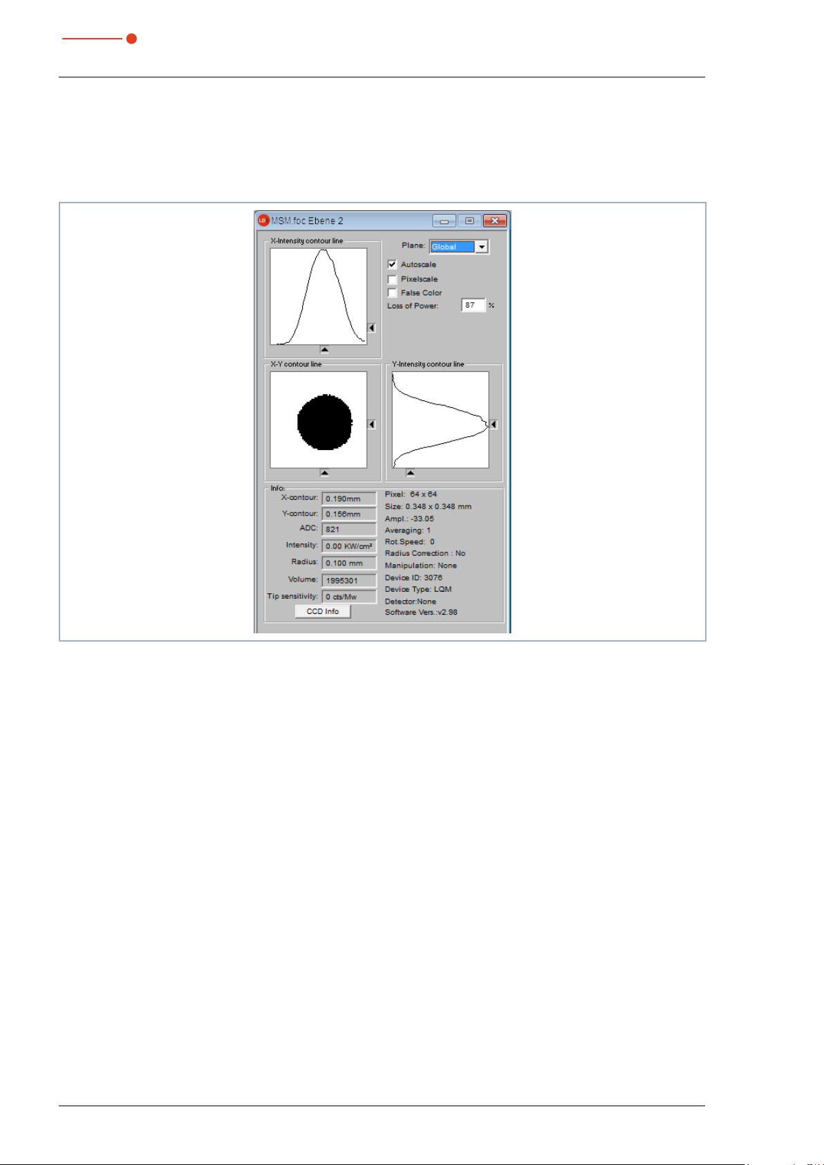
MicroSpotMonitor MSM
35,0(6
12.5.10 Variable contour lines (menu Presentation > Variable Contour Lines)
Here the spatial power density distribution is displayed by means of freely selectable contour lines. Not only
intersections in x- and y- direction but also in power density coordinates (A/D-converter-counts) can be carried out. The position of the intersections is settable by means of a slide control or the keyboard.
Fig. 12.29: Dialoque window Variable contour lines
Setting by means of the keyboard:
• For the x-direction by means of the key x in order to increase the value and <shift>x in order to de-
crease it.
• For the y-direction by means of the key y in order to increase the value and <shift>y in order to de-
crease it.
• For the power density (intensity) by means of the key i in order to increase the value and <shift>i in
order to decrease it.
In the range of the left hand lower corner the current intersection coordinates, the power densities, the radius
generated by the intersection as well as the relative volume are displayed. The values are calculated basing
on the correctly entered laser power.
In the right hand upper corner it is possible to switch the scaling. Below it, there is an input field where the
desired power loss (-inclusion) can be entered. This value correlates to the given power levels in the window.
In addition to these functions, this window also offers plenty of additional information on the conditions under
which measurements are taken. The amplification, resolution number, and the software version used for
measuring are all displayed while measuring as well.
70
Revision 01/2019 EN

MicroSpotMonitor MSM
35,0(6
One click on the CCD Info button will open a window with additional information on the device parameters
such as trigger mode, trigger delay, integration duration, magnification, and focussing optic type.
Fig. 12.30: Display window CCD Info
Revision 01/2019 EN
71

MicroSpotMonitor MSM
35,0(6
12.5.11 Graphical review (menu Presentation > Graphical Review)
The display window Graphical review offers many possibilities to display the measurement values of the
single measurement planes. In total this window can present 20 different graphs. The possible selections for
the x- and y-coordinates are shown in the Tab. 12.7 on page 72.
y-axis x-axis
Radius Power
x-position Time
y-position Plane
Angle Position
Ellipticity
Tab. 12.7: Selections for the x/y coordinates
Fig. 12.31: Display window Graphical review – Example for assessment of a time series - radius/time
See chapter 12.4.9 on page 54, Section „Manual caustic measurement as time series (menu Measurement > Caustic > Manually adjusted)“.
12.5.12 Systemstate (menu Presentation > Systemstate)
Not relevant for MicrosSpotMonitor MSM.
72
Revision 01/2019 EN

MicroSpotMonitor MSM
35,0(6
12.5.13 Evalution parameter view (menu Presentation > Evalution Parameter View)
In the directory “System“ in the LDS installation file (C:\Program\Primes\LDS2.98\System) you can find
predefined parameter files for the raw beam retrograde calculation (RawBeamParams.eval) and the caustic
evaluation (beamparams.eval). These can be pulled up under the menu point Presentation > Evaluation
Parameter View.
Fig. 12.32: Display window Evalution Parameter View with opened parameter file
The desired parameters and their limit values can be stipulated by means of the program PRIMES-EvalEditor
and can then be saved in the evaluation parameter file (*.eval). The program is automatically installed when
the LDS-setup is carried out.
Fig. 12.33: Dialoque window EvalEditor with loaded *.eval-file
Revision 01/2019 EN
73
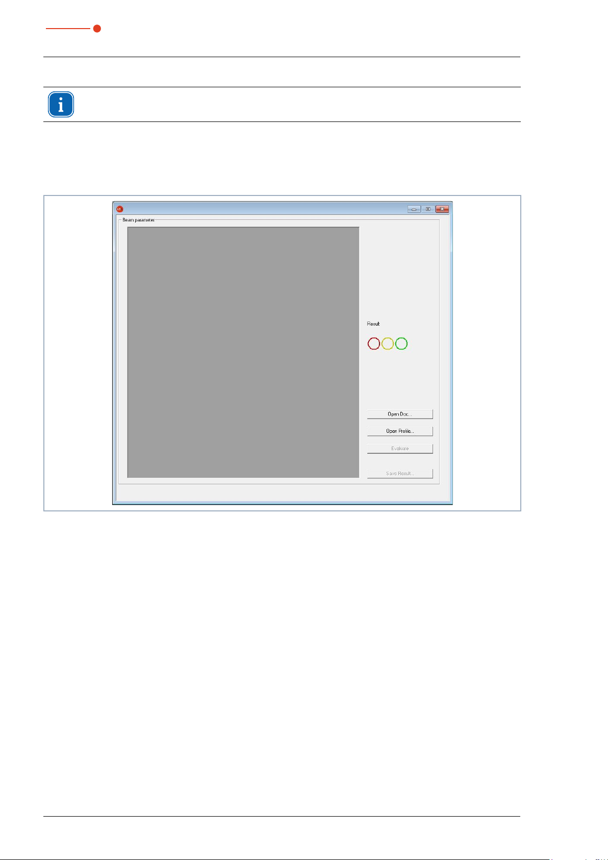
MicroSpotMonitor MSM
35,0(6
The evaluation parameter file can only be displayed if the file BeamControls.xsd is located in the
same directory (C:\Program\Primes\LDS2.98\System)!
12.5.14 Evaluate document (menu Presentation > Evaluate doc)
The evaluation function compares selectable beam parameters and their adjustable limit values with the
results of a current or a saved measurement.
Under the menu point Presentation > Evaluate doc of the LDS, the following dialog window is opened:
Fig. 12.34: Dialoque window Evaluate Document for loading an evaluation file
The button Open Doc opens a file selection window that allows to choose a saved measuring file (*.foc).
The button Open Profile opens a file selection window for choosing an evaluation parameter file (*.eval).
The button Evaluate triggers an evaluation (see Fig. 12.35 on page 75). The single evaluation parameters
and the result of the evaluation are displayed. The overall evaluation (Result) of all results is displayed by
means of a traffic light symbol.
74
Revision 01/2019 EN

MicroSpotMonitor MSM
35,0(6
Evaluation Criteria: Only if all single evaluations are ok, the overall evaluation is displayed in green in the traffic
light symbol.
Fig. 12.35: Dialoque window Evaluate
In case the warning or limit values are exceeded, this has an influence on the color display of the traffic light
symbol. As soon as a warning value is exceeded or fallen short of, the yellow circle is filled. If the limit values
(min/max) are exceeded or fallen short of, the red circle is filled. The actual values in the table of the evaluation window are marked in color as well.
Green YellowYellowRed Red
(−)
0WarnMin MaxWarn
Fig. 12.36: Traffic light colors when warn- and limit values are exceeded
The overall result of the evaluation can be saved by means of the button Save.
Traffic light color
Limit values(+)
Revision 01/2019 EN
75

MicroSpotMonitor MSM
35,0(6
12.5.15 Color tables (menu Presentation > Color Tables)
Different color charts are available. It is possible to switch back and forth between the color charts. Thus the
assignment of A/D converter values and different color scales can be varied. This is important for the false
color presentation.
Three settings are possible:
• Linear color table (basic setting)
• Color table analogue to the root function
• Color table analogue to the fourth root function
These functions can especially be helpful as far as the analysis of slight variations near the zero level are concerned; e.g. the analysis of diffraction phenomena.
Fig. 12.37: Dialoque window Color Setup – Linear color table and 2nd root color table
12.5.16 Toolbar (Menu Presentation > Toolbar)
The toolbar can be shown or hidden by clicking Presentation > Toolbar in the menu.
Fig. 12.38: Showing or hiding the toolbar
76
Revision 01/2019 EN

MicroSpotMonitor MSM
35,0(6
12.5.17 Position (menu Presentation > Position)
This menu can be used to move the device to its parked position.
Fig. 12.39: Dialoque window Postition
12.5.18 Evaluation (option) (menu Presentation > Evaluation)
By means of this evaluation function, you can compare and evaluate different parameters of the measured
caustic (.foc-file) with specified limit values (.pro-file). The evaluation result is displayed optically with an LED
symbol (red=bad, green=good). The overall result (field Conclusion) is only considered as good provided that
all results are within the critical parameters (
).
Fig. 12.40: Dialoque window Evaluation
The parameters, the limit values and the identification of critical values are purported in a profile file (text file,
please see the example file in Fig. 12.41 on page 78).
Revision 01/2019 EN
77

35,0(6
Fig. 12.41: Example for a profile file
MicroSpotMonitor MSM
An evaluation is carried out as follows:
1. Click the button Open Doc and choose your measuring file (.foc-file).
2. Click the button Open Profile and choose your profile file (.pro-file).
3. Choose the desired radius definition in the selection Caustic.
4. Click on the button Evaluate.
78
Revision 01/2019 EN

MicroSpotMonitor MSM
35,0(6
12.6 Communication
12.6.1 Rescan bus (menu Communication > Rescan bus)
This menu can be used to reconnect a device that was connected previously.
12.6.2 Free communication (menu Communication > Free Communication)
By means of this menu you can control the communication via the PRIMES bus. Moreover, the settings for
the communication are made here (see chapter 11.3.2 on page 31).
Fig. 12.42: Dialoque window Communication > Free Communication
Revision 01/2019 EN
79

MicroSpotMonitor MSM
35,0(6
12.6.3 Scan device list (menu Communication > Scan device list)
Every PRIMES device has a certain bus address. If a device is supposed to be controlled by means of the
LaserDiagnosticsSoftware LDS, the address has to be entered here. Moreover addresses can also be added
or deleted in this menu.
Fig. 12.43: Dialoque window Scan device list
The following addresses for all PRIMES devices may be listed in the device list:
80, 92, 112, 113, 114, 144, 145, 152, 161, 168
For the MicroSpotMonitor MSM, the address 161 must be entered.
80
Revision 01/2019 EN
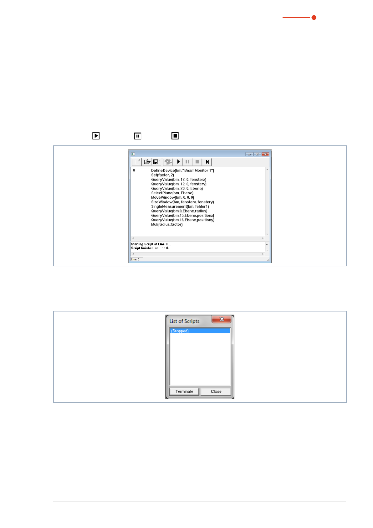
MicroSpotMonitor MSM
35,0(6
12.7 Script (menu Script)
By means of scripts complex measurement procedures can be controlled automatically. Scripts are programs which are written in several script languages. Scripts are almost exclusively provided as source files in
order to enable an easy editing and adjustment of the program.
12.7.1 Editor (menu Script > Editor)
By means of the script editor you can draw up scripts which can control, for example, complex measuring
procedures automatically. An example is given in Fig. 12.44 on page 81 – the beam find procedure with
the MicroSpotMonitor MSM.
In order to open the script, the Open symbol has to be clicked, then a file can be chosen and played by using the button
. The button stops and ends the script.
Fig. 12.44: Dialoque window Script – Script for the beam find procedure of the MicrosSpotMonitorMSM
12.7.2 List (menu Script > List)
Here all available scripts are listed.
Fig. 12.45: Display window List of Scripts
12.7.3 Python (menu Script > Python)
Starts the Python editor. The graphical user interface is identical to the one depicted in Fig. 12.44 on page
81. Python is a programming language with efficient abstract data structures and a simple but effective
approach for an object-oriented programming. Python is not only suitable for scripts but also for a fast application development. For programming with Python a separate PRIMES documentation is available.
Revision 01/2019 EN
81

35,0(6
13 Measurement
13.1 Safety instructions
DANGER
Serious eye or skin injury due to laser radiation
During the measurement the laser beam is guided on the device, which causes scattered or
directed reflection of the laser beam (laser class 4). The reflected beam is usually not visible.
The MicroSpotMonitor MSM must not be operated in any of the available configurations
without taking the following precautions.
Please wear safety goggles adapted to the power, power density, laser wave length and
X
operating mode of the laser beam source in use.
Wear suitable protective clothing and protective gloves.
X
Protect yourself from laser radiation by separating protective devices (e.g. by using appro-
X
priate shielding).
MicroSpotMonitor MSM
DANGER
Serious eye or skin injury due to laser radiation
If the device is moved from its calibrated position, increased reflected radiation
(laser class 4) may result during measuring operation.
When mounting the device, please ensure that it cannot be moved, neither due to an unin-
X
tended push or a pull on the cables.
NOTICE
Damaging/destroying the device
Contamination and fingerprints on the protective window can lead to damage or shattering
or splintering of the protective window during measuring operation.
Do not touch the protective window.
X
Regularly check the condition of the protective window and exchange it in case of pollution
X
(see chapter15.1, „Exchanging the protective window“, on page109).
Only operate the device with a clean protective window.
X
NOTICE
Damaging/destroying the device
Obstacles in the movement range of the MicroSpotMonitor MSM can lead to collisions and
damage the device.
Keep the movement range free of obstacles (cutting nozzle, pressure rolls, etc.).
X
82
Revision 01/2019 EN

MicroSpotMonitor MSM
35,0(6
1 10 100 1000
NOTICE
Damaging/destroying the device
Contamination can damage or destroy the optical components.
Only open the device in a dust-free environment.
X
13.2 Selection and change of measuring objectives
13.2.1 Selection of the measuring objective
The selection of the right measuring objective is of crucial importance when it comes to the quality of the
measurement with the MicroSpotMonitor MSM.
The measuring objective must be optimally matched to the wavelength, the numerical aperture and the focus
size to be measured. Furthermore, the possible fields of application are limited by the sensor- and pixel size
(see chapter 21.4.1 on page 121).
10x + BPE
10x
5x + BPE
5x
3.3x + BPE
3.3x
1 10 100 1000
Focus diameter in µm
Fig. 13.1: Fields of application of the measuring objectives
In Fig. 13.1 on page 83 the field of application of different measuring objectives is depicted. The figure allows a quick first selection of the correct measuring objective.
Revision 01/2019 EN
83

MicroSpotMonitor MSM
35,0(6
The following table contains the limits that have to be observed when it comes to standard objectives as well
as further objective data.
Standard
Objective NA F Max. measuring window Min. resolution Min. beam diameter Max. beam diameter
3.3x 0.1 5 1.4mm 1.4 μm 30μm 1mm
5x 0.2 910μm 0.9μm 20μm 650μm
10x 0.2 2 510μm 0.5μm 11μm 350μm
With beam path extension (BPE)
Objective NA F Max. measuring window Min. resolution Min. beam diameter Max. beam diameter
3.3x 0.1 5 800μm 0.8μm 17.5μm 550μm
5x 0.2 550μm 0.5μm 12μm 380μm
10x 0.2 2 320μm 0.3μm 7μm 220μm
With alignment objective (AO)
Objective NA F Max. measuring window Min. resolution Min. beam diameter Max. beam diameter
3.3x 0.1 5 4mm 3.9µm 90µm 2.8mm
5x 0.2 2.75mm 2.7µm 60µm 2mm
10x 0.2 2 1.6mm 1.6µm 35µm 1.1mm
Tab. 13.1: Measuring objective data
NA = numerical aperture
F = focusing value (see Fig. 13.5 on page 87)
On the basis of this table, a suitable measuring objective can be selected. The values apply for a wavelength
of 1 064nm (the values slightly differ with other wavelengths).
84
Revision 01/2019 EN

MicroSpotMonitor MSM
35,0(6
13.2.2 Exchanging the measuring objective
1. Unscrew the two knurled screws (see Fig. 13.2 on page 85).
2. Remove the measuring objective upwards.
• Please note that the measuring objective is fixed by two dowel pins and does not tilt during removal.
Knurled screws
Dowel pins 2x
Fig. 13.2: Measuring objective
NOTICE
Component susceptible to electrostatic discharge
The EEPROM can be destroyed by an electrostatic discharge.
Do not touch the contacts of the EEPROM as well as the contact pins (see Fig. 13.3 on page 85).
X
Put on an ESD armband before changing the measuring objective.
X
There is an EEPROM in the mount of the measuring objectives, which contains all the objective data necessary.
Contact pins
Dowel pins 2x
Fig. 13.3: Measuring objective – contacts and contact pins
3. Place the measuring objective from above on the two dowel pins (see Fig. 13.2 on page 85).
4. Press the measuring objective vertically down to its stop.
• When inserting, make sure that the measuring objective does not tilt.
Revision 01/2019 EN
85

MicroSpotMonitor MSM
35,0(6
13.2.3 Damage thresholds
The operating limits of the MicroSpotMonitor MSM are determined by the damage thresholds of the optical
components. As described in chapter 21.4.1 on page 121, two different cases have to be considered.
NOTICE
Damaging/destroying the measuring objective
Power densities which are too high can destroy the measuring objective.
Please mind that the power density I is smaller on the first lens
X
~10MWatt/cm²(cw) or ~100MWatt/cm² (pulsed) respectively.
The medium power should not exceed 250 Watt.
X
The power density I is calculated according to the following formula:
Fig. 13.4: Formula for calculating the power density I
• If the focus is placed below the measuring plane (too close to the measuring objective), the power den-
sity rises at the first lens of the measuring objective.
• If the focus is above the measuring plane, an intermediate focus develops inside the device. If the laser
beam focus is too far above the measuring plane, the intermediate focus can develop in areas in which
the beam power has not been sufficiently decreased. This can damage the image-sided beam path.
The size and position of the range in which the focus is to be positioned before the first measurement depends on the measuring objecive selection, the used wavelength as well as on the type of focusing.
The diagram in Tab. 13.2 on page 87 shows that the upper limits for high-magnification measuring objectives are much narrower than those with a 3.3-fold magnification.
The lower limit for convergent beams depends on the power density of the laser beam on the first lens. This
is a function of the laser power, the focusing, the M², as well as the raw beam diameter.
86
Revision 01/2019 EN

MicroSpotMonitor MSM
35,0(6
The graphs in Tab. 13.2 on page 87 and Tab. 13.3 on page 88 can be used to estimate the minimum
distance.
Measuring plane distance
PRIMES 10x-h without BPE
Measuring plane distance
PRIMES 3,3x-s without BPE
5
4,5
F = 5
4
3,5
3
2,5
2
1,5
Beam radius on the first lens in mm
1
0,5
0
20
Tab. 13.2: Estimatation by the focusing value F for 1 064 nm and 532 nm
30 40 50 60 70 80
Distance between focus and measuring objective in mm
F = 10
F = 15
F = 20
F = 30
The diagram in Tab. 13.2 on page 87 shows the dependence of the beam radius on the first lens with the
focusing value F and the distance of the focus from the first lens of the measuring objective.
The focusing value F can be determined by means of the following formula:
Fig. 13.5: Formula for calculating the focusing value F
f = Focal length of the focusing lens
ds = Raw beam diameter
Θ = Full divergence angle
Revision 01/2019 EN
87

35,0(6
530 nm 1064 nm
52,5
42
MicroSpotMonitor MSM
Measuring plane distance
PRIMES 10x-h without BPE
Measuring plane distance
PRIMES 3,3x-s without BPE
w0 = 5μm
M² = 1
w0 = 8μm
31,5
21
10,5
Beam radius on the first lens in mm
00
20
Tab. 13.3: Estimatation by the focus radius for 1064nm and 532nm
30 40 50 60 70 80
Distance between focus and measuring objective in mm
w0 = 10μm
w0 = 15μm
w0 = 30μm
w0 = 50μm
The diagram in Tab. 13.3 on page 88 shows the dependence of the beam radius on the first lens with the
wavelength, the focus radius, and the distance of the focus from the lens.
The beam radii are estimated by means of the beam parameter product BPP.
Fig. 13.6: Formula for calculating the beam radii by the beam parameter product BPP
w
= Beam radius
0
Θ = Full divergence angle
λ = Wavelength
M2 = Beam quality factor
In Tab. 13.3 on page 88, the beam quality factor M² was assumed to be 1.
The dependencies can be summarized as follows:
• When it comes to strongly divergent beams, e.g. with a focusing with small focal lengths, small focus
radii develop. In order to be able to achieve a sufficient resolution on the camera chip, the 10-fold measuring objective is necessary. This objective also has a greater numerical aperture.
• When it comes to laser beams with a beam quality factor M² = 1-2, small focus radii also occur with
small divergences. This may lead to damages of the entry lens when long focal length objectives are
used.
• When it comes to laser beams with large beam quality factor M² values, high power values occur. They
are, however, not so critical due to the large focus radii. The spot diameter on the entry lens should
always be greater than 1mm.
88
Revision 01/2019 EN
MicroSpotMonitor MSM
35,0(6
13.3 Prepare measurement
The following check lists should help you to realise the most important conditions for a measurement and to
carry out all necessary settings of the LaserDiagnosticsSoftware LDS.
13.3.1 Check list measurement settings
The device is stable and fixed.
The movement range (z-axis) of the measuring device is free of obstacles.
Tab. 13.4: Check list safety precautions
13.3.2 Check list measurement settings
LDS Menu Path Action
Measurement > Environment
Measurement > Sensor parameters
Measurement > CCD Settings
Measurement > Single
Measurement > Caustic
Measurement > Option
Tab. 13.5: Checkliste Messeinstellungen
Enter the focal length
Preset 64 pixel for the resolution x
Preset 64 pixel for the resolution y
Select the trigger mode Cw/Quasi-cw Measurement
Select the CCD mode Measuring data
Select the correct wave length
Activate the checkbox Optim.
Activate the mode Automatic
Activate the checkbox Optim.
Preset the fillfactor Max: 0.7 Min: 0.5 Ref: 0.6
Analyse Settings: Activate the checkbox Enable adjust nullevel
Revision 01/2019 EN
89
35,0(6
13.4 Flowchart of a measurement
13.4.1 Prepare measurement
MicroSpotMonitor MSM
Preparation
Positioning z-axis:
MSM 35 = 18mm
MSM 120 = 60mm
Select Magnification
Low x 0.3
on the device
Set laser power on
minimum
1. mea-
surement
with largest
window
13.4.2 Set caustic limits
No
Focus
found?
Check alignment
again
Laser beam is
switched on?
OD filter is
selected?
Yes
Increase laser
power
Too
low
Search caustic
Check
saturation
S/N
Too high
Increase
filter
settings
ok
Decrease z-axis value
until the beam fits the
biggest window
Beam gets bigger
Increase
z-axis value
Beam gets smaller
Increase the z-axis value
until the beam fits to the
biggest window
Lower limit value for the
caustic measurement
found
Search caustic
settings
Beam fits
No Yes
into the
biggest win-
dow
Increase z-axis value
until the beam fits into
the biggest window
Increase z-axis value
until the beam fits into
the biggest window
Upper limit value for the
caustic measurement
found
Upper limit value for
the caustic measure-
ment found
Decrease the z-axis
value until the beam fits
to the biggest window
Lower limit value for
the caustic measure-
ment found
Start first
caustic measure-
ment
90
Revision 01/2019 EN
MicroSpotMonitor MSM
35,0(6
13.4.3 Perform caustic measurement
First
caustic measure-
ment
Enter caustic limit
values
Start measuring
program
Increase
laser power
Start
caustic measurement
Set caustic limits
±3z
around the focus
R
Set number of mea-
surement planes to 21
Open
new file
Start
measurement
> 6z
Check
R
measurement
range
< 6z
Carry out asymmetric
measurement
−3z
to +1z
R
R
Limited by
Yes
R
z-axis
No
Revision 01/2019 EN
91

MicroSpotMonitor MSM
35,0(6
13.5 Perform measurement settings in the LaserDiagnosticsSoftware LDS
The following explanations of the configuration options should help you to make the right settings for the
respective task.
The following chapters highlight important configuration options in color:
Color Meaning
Red This setting must always be set as shown.
Yellow This setting is dependent from the desired operating mode (CW, pulse, single pulse, measurement
Green This setting must be carried out before each measurement. The settings depend on the specific mea-
Tab. 13.6: Color meaning of the setting options
series, etc.).
surement task, such as the wavelength, the laser power or the geometry of the laser beam.
92
Revision 01/2019 EN

MicroSpotMonitor MSM
35,0(6
13.5.1 Sensor parameters (menu Measurement > Sensor parameter)
Adaptable squares
Z
Y
Fig. 13.7: Dialogue window Sensor parameters
Mechanical limits
By pulling the turquoise square with the mouse pointer you can restrict the movement range of the y- and zaxis. Therewith you can prevent damages in case other components reach into the movement range of your
device. The maximum value corresponds to the value Y3 and Z3.
Resolution
Here you can enter the number of pixels in the measuring window, ranging from 32x32 to 256 x 256 pixels.
Generally, 64 pixels per line and a total of 64 lines is sufficient. Please keep in mind that the more pixels there
are, the longer the measurement will take.
Manual z-axis
With this function you can deactivate the z-axes of the measuring system. This is useful if you want to use
external movement axes. In this case you can manually assign a z-value to every measurement plane in the
dialogue window Single measurement.
Please find further information on the menu Menu Measurement > Sensor paramter in chapter 12.4.2
on page 45.
Revision 01/2019 EN
93
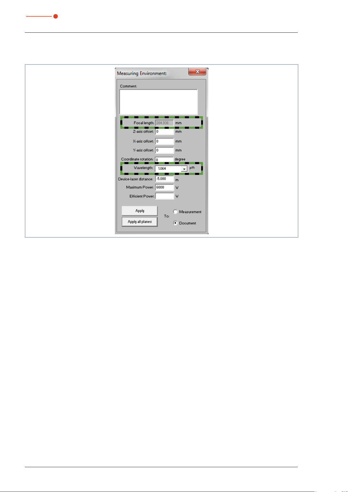
35,0(6
13.5.2 Measuring environment (menu Measurement > Environment)
MicroSpotMonitor MSM
Fig. 13.8: Dialogue window Measuring Environment
Focal length
Stating the focal length is relevant for the evaluation of the caustic measurements. From the caustic process
and the entered focal length the raw beam diameter on the focussing optic can be calculated.
Wave length
The wave-length is the basis for a correct determination of the beam quality factor M². There are the following options:
• 1.064 μm for Nd:YAG laser
• 0.532 μm for Green laser
• 0.355 μm for UV laser
A wavelength can also be typed in numerically.
Please find further information on the menu menu Measurement > Environment in chapter 12.4.1 on
page 44.
94
Revision 01/2019 EN

MicroSpotMonitor MSM
35,0(6
13.5.3 Measurement settings (menu Measurement > Single)
Fig. 13.9: Dialogfenster Messeinstellungen
Controlling measuring modes (individual measurement, monitor, and video mode)
There is a total of three different measuring modes that can be selected here. In the Individual Measurement and Monitor measuring mode, all necessary compensations (smear effect, diffusion) and exposure
time adjustments are performed every time a new measurement is carried out. Valid measuring data is generated in this mode.
The measuring mode VideoMode does not produce valid measurement data. Here the exposure time is
carried over from the last measurement and does not vary. Compensation measurements are not performed,
making it unnecessary to consider or compensate for measuring artifacts such as smear effects.
Due to the “high” measuring frequency of about 5 Hz, this operating mode is particularly suited for use when
aligning the device. The numeric results should not be interpreted absolutely, but rather always relative to
each other.
Optical amplification (opt. ampl.)
This function activates the automatic adjustment of the exposure time of the CCD for every measurement.
The function must be activated in order to keep the signal/noise ratio consistently high for a caustic measurement.
For special measuring applications, however, it might make sense to deactivate this function and set the exposure time to a fixed value between 12 µs and 200 ms. Here it is important to ensure sufficient attenuation
of the laser beam with the help of the fixed ND filter or the filter wheel.
Symmetrical
Once this function is activated, only rectangular measuring windows will be allowed. In cases where an elliptical or even a square laser beam is being measured, this function should be deactivated so that the measuring window can be optimally adjusted.
Please find further information on the menu Measurement > Single in chapter 12.4.8 on page 50.
Revision 01/2019 EN
95

35,0(6
13.5.4 Caustic settings (menu Measurement > Caustic)
Fig. 13.10: Dialogue window Caustic settings
MicroSpotMonitor MSM
Parameters (start number of the plane)
Under Start, the start number at which the measurement is initiated can be entered for the plane. By default,
the start number is generally set to zero and should only be changed when you are measuring in an existing
document and don’t want the existing measurement data to be overwritten. If, for example, you have measured a caustic with 21 planes and want to magnify the measuring area to the smaller z-values, you can set
the start plane to 21 and modify the measuring area appropriately. The new measuring values will then be
written into the existing document starting with plane 21.
In the Quantity selection field, the number of planes to be measured in the specified z range is set. The following should be considered here:
• Since the LaserDiagnosticsSoftware LDS always sets the measuring plane distances so they are equi-
distant (equal spacing) and the measuring area is almost always situated symmetrically around the focal
point, an odd number of measuring planes should be selected. The focus plane is calculated based on
the measuring plane and displayed in the caustic illustration.
• Beam measurement norm DIN 11146 specifies that at least 10 measuring planes should be measured.
Furthermore, five measurements should also be taken within a Rayleigh length and the other beyond 5
Rayleigh lengths. In order to meet all of the requirements with equidistant distribution, at least 17 measuring planes must be measured in a range of ± 3 Rayleigh lengths.
Mode (automatic and manual settings)
There are two different measuring modes for caustic measurement. In “Automatic” mode, the measuring
system and the LDS determine the ideal measuring window position (x- and y-direction) for each measuring
plane and the optimal measuring window size for the fill factor. Furthermore, the plane location in the z-direction is also calculated based on the specifications (number of measuring planes, measuring limits z-direction).
Especially when adjusting the measuring window size and the measuring window position in the xand y-direction, the number of iterations (max. three per plane) can result in an extended measurement duration.
It is therefore possible to change the measuring mode to “Manual Settings” for recurring measuring tasks
and for repeating measurements. In this case, the measuring system will take the measuring window positions and measuring window sizes from the previous measurement or from a .ptx file. This reduces the mea-
96
Revision 01/2019 EN

MicroSpotMonitor MSM
35,0(6
surement duration considerably, but does require that the location and parameters of the laser beam change
only minimally.
Beam search
This selection field specifies which plane the caustic measurement should be started in. If the optional Beam
Find function is activated in the Options dialog window, that is also the plane in which this function will be
performed. When the Beam Find function is deactivated, this plane must be manually measured ahead of
time to make sure that the laser beam is found.
Please find further information on the menu Measurement > Caustic in chapter 12.4.9 on page 54.
Revision 01/2019 EN
97

35,0(6
13.5.5 CCD settings (menu Measurement > CCD Settings)
MicroSpotMonitor MSM
Fig. 13.11: Dialogue window CCD Settings
The wavelength, attenuation, and operating mode are all set in the CCD Settings dialog window.
Trigger modes
The appropriate settings must be configured here in keeping with the operating mode of the laser to be measured. Here it is important to consider that pulsed lasers with a pulse frequency of more than 500 Hz can be
measured in cw mode. If, however, the operating mode is set to pulsed and a cw laser system is involved,
the measuring device will always display the error message “Error Black Pixel Measurement” or “Time Out
During Measurement” in reaction to a measurement request.
Delay
This function can only be used with a “triggered operation” trigger mode. The time the measuring system
should wait between when it detects the trigger pulse and the start of the measurement is set here. Together
with the function “Integration Duration”, defined “Windows” from the plus cycles can be measured (e.g. exactly one pulse or parts of an ms pulse. The minimum delay is 12µs.
CCD operating modes
Three different modes can be set here. If the Raw Data setting is activated, the measuring system will return
the uncompensated data of the CCD when a measurement is requested. Especially with NIR irradiation,
these can be riddled with measuring errors such as “smear effect” readout noise. Even the numeric beam
data generated generated from this data will be affected by this.
If a Background is selected as the operating mode, only correction data will be returned while measuring.
Measuring Data mode should always be the default setting here though. Only when this mode is turned on
can the measuring system deliver reliable measuring values.
98
Revision 01/2019 EN

MicroSpotMonitor MSM
35,0(6
Integration duration
This function sets a defined integration duration. The optimizer must be deactivated before this can be accomplished, since otherwise the measuring device itself will optimize and thus change the integration duration. This function is also used mainly in measuring pulsed laser systems.
Filter wheel
Which filter is needed for measuring depends on the wavelength and the intensity of the laser beam being
measured and the appropriate one must be chosen specifically for each measuring task.
A filter can be considered suitable when all measuring planes of a caustic measurement can be measured
using an exposure time between 18ms (-20dB) and 0.18ms (-60dB). Outside of these limits, the S/N ratio
of the CCD declines, thus reducing the accuracy.
Wavelength
Due to the wavelength-dependent overall magnification of the camera-based measuring system, it is important to check that the right selections have been made before each measurement. The wavelengths shown
here represent the calibration points of the measuring objective. As a result of the achromatic properties of
the measuring objective, a wavelength range between 1030 and 1100 can be achieved, for example, with a
calibration point at 1064 nm without causing generating measuring errors.
General sequence control
• Empty the CCD register
• Aim for the holding point in line a (line in which photo transfer takes place); if the trigger is set off during
sub-pulse, repeat line a (-> NLC = NoLineChange)
• Wait for the trigger if necessary and repeat line a (NLC)
• Wait out the delay if necessary and repeat line a (NLC)
• Aim for the holding point in line a through sub-pulse (-> delete the charge in the photo diodes)
• Integration – no cycles (sliding the charges through the register) of CCD
• Cycles start again, a few AD cycles later: Photo transfer
• Read out the CCD register; when the addresses match (= desired pixels), the measuring value is for-
warded to the AD transformer.
The various signals going through the transfer output mark certain points in time during the sequence control:
Transfer signals Meaning
Do transfer Is high when the CCD is at the holding point in line a (referred to in this way, since photo
Do transfer & Xend A short high-pulse, when we reach the end of line a.
Sub Is high as long as a sub-pulse is running.
Start done Is high when the CCD is ready for integration (or when waiting for the trigger) so when it
Wait for trigger Is high when the CCD is at the holding point in line a and is waiting for the trigger signal.
Integration done Is high as soon as integration is complete. Is low again when the CCD is read out.
Photo cycle Is high when the CCD is ready for integration. Is low as soon as integration is complete.
Tab. 13.7: Signals that can be sent through the transfer outlet
transfer also takes place in this line – when it isn’t being suppressed by the NLC).
is at the holding point in line a. Is low again when the CCD is read out. You could use the
positive side to light the laser.
Is low as soon as the trigger is activated and the delay begins. Only a short high pulse
occurs in untriggered operation. Could be used in addition to the trigger out connector to
check triggering.
During untriggered operation, the high phase returns exactly the integration time.
Please find further information on the menu Measurement > CCD Settings in chapter 12.4.5 on page 48.
Revision 01/2019 EN
99
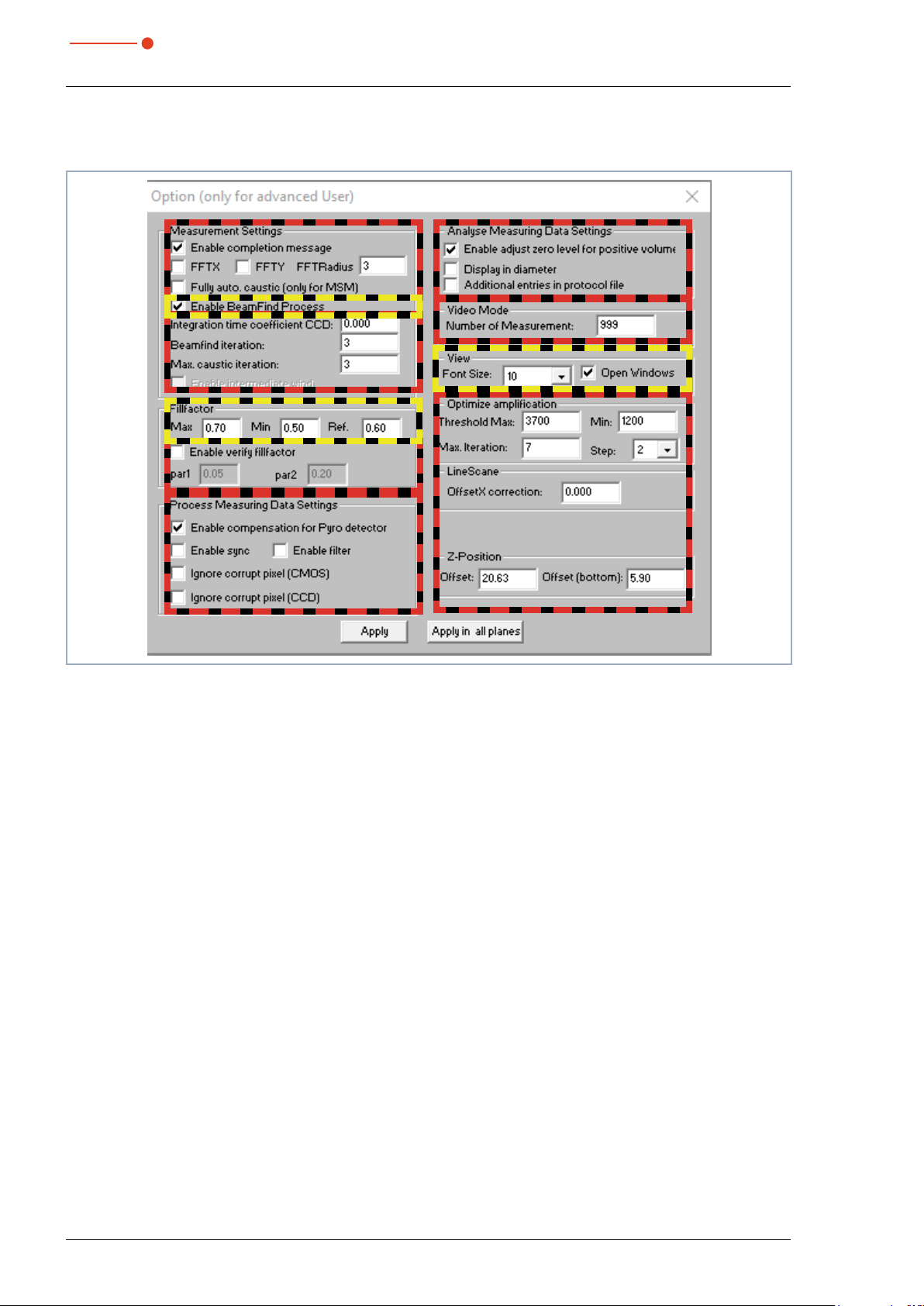
35,0(6
13.5.6 Option (advanced user only) (menu Measurement > Option)
MicroSpotMonitor MSM
Fig. 13.12: Dialog window Option
Enable beam find process
The Beam Find function must be used for caustic measurement. This involves an algorithm that separates
the measuring signal from the measurement artifacts (e.g. noise) via an adjustable trigger threshold and
adapts the size of the measuring window to this signal. This algorithm is only executed in the beam search
plane (Dialog window Caustic). On all other measuring planes, the measuring window size is determined using the fill factor.
If this function is deactivated, the beam search plane must be manually “premeasured” in the measuring
system. Otherwise the measuring system might end up positioning the measuring window on the edge of the
measuring area where there is no measuring signal. This makes it impossible to take a meaningful measurement.
If you turn the Beam Find function off and have the measuring measure the beam search plane system before each caustic measurement, you can save about 20 sec of measuring time per caustic measurement.
Summary: This function should be activated by default and only deactivated by experienced users. Turning
off this function can shorten the time for caustic measurements by about 15%.
Fillfactor
The fill factor is the quotient of the beam diameter and the length of the sides of the measuring window. As
long as the measuring signal is not cut off and there are no noise components in the measuring result and
now errors in the offset determination, the fill factor won’t influence the accuracy at all. But since every real
measuring signal is tainted with noise and since the precision with which the zero level of a measuring signal
can be determined is finite, very small fill factors can lead to a high level of accuracy. Depending on how
substantial the RMS noise is and the errors in the zero level determination of a measuring plane, the optimal
fill factor value to produce the best possible mathematical result will be different.
100
Revision 01/2019 EN
 Loading...