Pico Technology PQ187 User Guide

Download

PQ186 Network Metrology Training Kit

Including optional PQ187/PQ188 Standard and Premium Demonstrator Kits

User’s Guide

Network Metrology Traning Kit User’s Guide

Contents

1 Overview ................................................................................................................................................. 3

2 Kit contents ............................................................................................................................................ 4

2.1 PQ186 Network Metrology Training Kit Contents ....................................................................... 4

2.2 PQ187 Standard Demonstrator Kit Contents............................................................................... 5

2.3 PQ188 Precision Demonstrator Kit Contents .............................................................................. 5

3 Preparation ............................................................................................................................................. 6

3.1 Preparation to use the PQ186 Network Metrology Training Kit ................................................. 6

3.2 Preparation to use the PQ187 or PQ188 Network Metrology Demonstrator Kits ..................... 7

4 VNA calibration ...................................................................................................................................... 8

4.1 VNA Calibration using the PQ190 Low Cost SMA(f) Calibration Kit .......................................... 8

4.2 VNA calibration using the PQ186 NMT KIT PCA on-PCB SOLT standards ............................... 9

4.3 VNA Calibration using the PQ187 or PQ188 Demonstrator SMA(f) or PC3.5(f) Calibration Kits 9

4.4 To calibrate or compensate feedlines? ...................................................................................... 10

5 Applying reference plane shift to compensate feedline length. ....................................................... 11

6 Applying normalization to compensate feedline loss ....................................................................... 13

7 Applying de-embed to compensate feedline length, loss and port match. ...................................... 15

8 Measuring the on-PCB example networks ......................................................................................... 17

8.1 Measuring the on-PCB Calibration Thru Example ..................................................................... 17

8.2 Measuring the on-PCB Low Pass Butterworth Filter Example .................................................. 18

8.3 Measuring the on-PCB Attenuator example .............................................................................. 19

8.4 Measuring the on-PCB Bandpass Butterworth Filter example ................................................. 20

8.5 Measuring the on-PCB –6 dB Power Divider (time domain reflection) example..................... 22

8.6 Measuring the on-PCB 0603 surface mount component location. .......................................... 25

8.7 Measuring the on-PCB broadband amplifier example .............................................................. 26

8.7.1 Measuring the on-PCB broadband amplifier example – measure and de-embed the

“insertable” output attenuator. ............................................................................................................ 30

8.7.2 Measuring the on-PCB broadband amplifier example – calibrate to include an output

attenuator as part of the test feed. ..................................................................................................... 35

8.8 Measuring the non-linearity characteristic and the P1dB compression point of the on-PCB

amplifier .................................................................................................................................................... 37

8.9 Measuring level-dependent phase shift (AM to PM) of the on-PCB amplifier ......................... 40

8.10 The mismatched Beatty line example – verifying a calibration and measurement setup ...... 41

8.10.1 Verifying a calibration and measurement setup in terms of absolute accuracy ............ 43

Network Metrology Traning Kit User’s Guide

1 Overview

The PQ186 Network Metrology Training (NMT) kit is designed to support learning, practice and experience of RF and microwave network measurements in the sub-6 GHz frequency range. The trainer or student needs only a Vector Network Analyzer and this NMT kit to start performing calibration and network measurement tasks. Suitable N and SMA adapters, calibration standards, test leads and fixed wrenches are all included, and these are all of sufficiently low replacement cost that occasional misuse and even damage can be tolerated at an early stage of learning.

Unsurprisingly, Pico recommends the use of low-cost, high-performance PicoVNA instruments with these kits, but other VNAs with either N-type or SMA compatible ports could be used.*

Two optional Network Metrology Demonstrator kits comprise either PQ187 SMA (standard) or PQ188 PC3.5 (premium) test leads, calibration standards and a Pico verification standard. With these kits the full professional measurement capability of a PicoVNA (or any other VNA) can be realized and verified. This might for example achieve dual purposing of the VNA investment both in the classroom and in the research project requiring accurate and traceable measurement. It is also envisioned that the demonstrator kit can facilitate the evaluation and discussion of measurement errors that may have been encountered whilst using the student NMT kit and its lesser standards and test cables.

* Scalar network or time domain reflectometry instruments may also be used with these kits.

Network Metrology Traning Kit User’s Guide

2 Kit contents

2.1 PQ186 Network Metrology Training Kit Contents

Item

Order Code / File Name

Description

Qty

PQ189

TA435 NMT kit printed circuit assembly supplied in carry case

Containing: Feedline end SOLT calibration standards. Mismatched 25 Ω Beatty Line. 0603 chip component test location. Lowpass Butterworth filter. Bandpass Butterworth filter. Attenuator. –6 dB Power divider. 6 GHz Broadband amplifier (requires external +5 V DC supply).

PQ190

SMA(f) short, load and open/thru low-cost calibration kit (3 items)

TA314

N(m)–SMA(f) inter-series adaptor

TA312

SMA(m-m) 600 mm test lead

TA484

SMA(m-m) within-series adaptor

TA482

SMA(f-f) within-series adaptor

TA486

PicoWrench RF N+SMA connectors multitool

8 On USB stick or download

Folder containing: NMT kit default set.sta

NMT kit default calibration (at SMA).cal Ideal SOLT.kit NMT kit typ SOLT SMA(f) Vx.kit

NMT kit meas de embed port1.s2p NMT kit meas de embed port2.s2p

NMT kit Users Guide.pdf

Available from www.picotech.com/downloads

Recommended default settings for use with this kit.

(other settings called by this guide are also provided)

Default typical calibration & settings, SMA(f) referenced ‘Ideal’ lossless, zero length calibration kit data **. Typical calibration kit data for low-cost SOLT SMA(f) **.

Measured ‘typical’ de-embed Touchstone file for the NMT kit PCA feedlines.

This User’s and Trainer’s guide in PDF format.

** Calibration kit data in PicoVNA .kit format and also as 4x Touchstone (Open.s1p, Short.s1p, Load.s1p and Thru.s2p).

Network Metrology Traning Kit User’s Guide

2.2 PQ187 Standard Demonstrator Kit Contents

Item

Order Code

Description

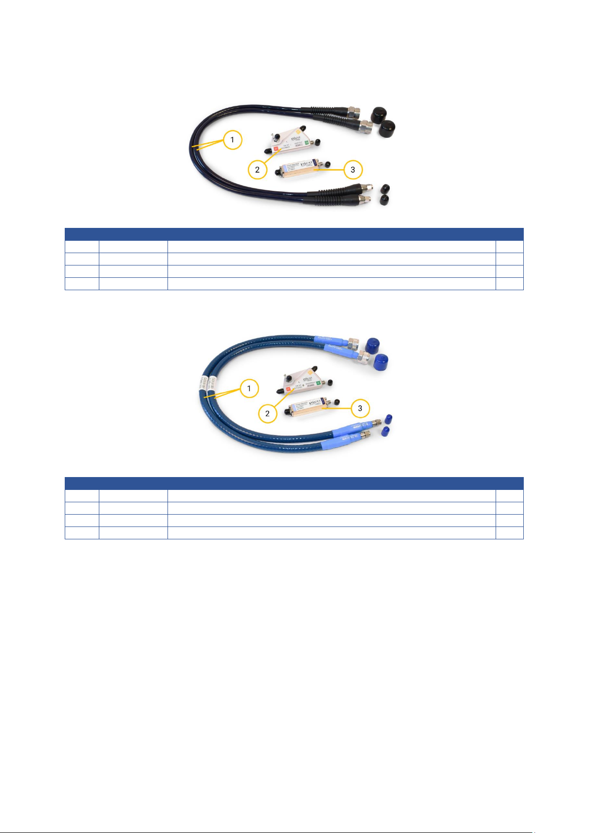
Qty 1 TA336

N(m)–SMA(m) standard VNA test Lead

TA345

Standard SMA(f) SOLT calibration kit with data

TA431

SMA(f-f) non-insertable check standard and data

1 n.a.

Serial-number-specific data for TA431 and TA345 on USB stick

2.3 PQ188 Precision Demonstrator Kit Contents

Item

Order Code

Description

Qty 1 TA338

N(m)–PC3.5(m) premium VNA test Lead

2 2 TA347

Premium PC3.5(f) SOLT calibration kit with data

1 3 TA431

SMA(f-f) non-insertable check standard and data

1 n.a.

Serial-number-specific data for TA431 and TA347 on USB stick

The remainder of this guide assumes a working knowledge of the PicoVNA or alternative VNA in use. For calibration or operation guidance please see the relevant instrument user guides.

Network Metrology Traning Kit User’s Guide

3 Preparation

3.1 Preparation to use the PQ186 Network Metrology Training Kit

On the USB memory stick, or available for download in updated form at www.picotech.com, you will find this guide and other user files in the folder:

NMT kit User Guide and Files Vx.xx.

For PicoVNA users it will be convenient to copy and paste the Pico-recommended default calibration and settings files “NMT kit default calibration (at SMA).cal”, “NMT kit default settings.sta” and all similar .cal and .sta files into the folder:

User: Documents/PicoTechnology/PicoVNA2/

The measurement setup that we use with Network Metrology Training Kit varies with test or set of tests being performed, personal preference and possibly with the VNA that is being used. However, there is a kick-off instrument status that Pico recommends for its PicoVNA. The setup is suited to include time domain display capability and uses a resolution bandwidth suited to any of the measurements that students are likely to make with this training kit.

The settings summary is:

• 2048-point (TD) sweep 2.93 MHz to 6010 MHz at –3 dBm port power

• 12-term non-insertable known thru calibration

• 1 kHz resolution bandwidth

• Markers on (5), Active Channel 3

• Display Ch1 – S11 Log Mag, 5 dB/div, Ref 0 dB at grat 2

• Display Ch2 – S21 Log Mag, 0.5 dB/div, Ref 0 dB at grat 2

• Display Ch3 – S11 TD (Hann), 0.2 U/div, Ref 0 U at grat 3, timebase span –1 ns to 9 ns

• Display Ch4 – S22 Log Mag, 5 dB/div, Ref 0 dB at grat 2

These settings are provided for the PicoVNA within the download instrument status file:

NMT kit default set.sta

The settings are also recalled within a default calibration and status file. This will establish a typical calibration and default settings. The setup should be recalibrated whenever this is used:

Network Metrology Traning Kit User’s Guide

NMT kit default calibration.cal

Also supplied and conveniently transferred to their target folder are the calibration kit data .kit files. These should be copied into the “Calkits” folder:

User: Documents/PicoTechnology/PicoVNA2/Calkits

The supplied PicoVNA .kit files are ideal data for the on-PCB and typically measured data for the low-cost SMA(f) calibration standards provided with this training kit. Files of the same version number are all identical and can be used with any NMT KIT PCA or SMA(f) kit of the same appearance (as shown below).

Note: The full specified measurement accuracy of the PicoVNA, or any other VNA that is calibrated with these low-cost standards and their ideal or typical data, will not be fully realized. Measurement uncertainties will be significantly increased but tolerable within the training environment.

Note: Calibration Kit data that accompanies any other Pico-supplied calibration kit (those within the PQ187 and PQ188 demonstrator kits for example) is specific and unique to the serial number of the kit it represents. This very specific data for a kit can realise the full specified accuracy in any measurement. It is also possible using these high-performance standards to measure lesser SOLT devices and then to create calibration .kit files for the PicoVNA. The method is described in Appendix 2.

Users of other VNAs can use the Touchstone data files provided for each of the standards onPCB or SMA(f). Alternatively the near-equivalent polynomial models for the standards are provided in the table below.

Cal’ Std.

Offset / Length (mm)

Loss (GΩ/s)

C0 (10

-15

)

C1 (10

-27

)

C2 (10

-36

)

C3 (10

-45

)

L (pH)

PQ190 Low-cost SMA(f) Calibration Kit typical models V1

Open

16.8

17.5

30 0 0 0 n.a.

Short

14.4

16.5

n.a.

Thru

19.4

n.a.

Ideal lossless, zero-length models

Open 0 0 0 0 0 0

n.a.

Short 0 0

n.a.

Thru 0 n.a.

n.a.

3.2 Preparation to use the PQ187 or PQ188 Network Metrology Demonstrator Kits

For PicoVNA users it will be convenient to copy and paste the calibration kit data.kit file and the

check standard.s2p files from the included USB memory stick to the respective “Calkits” and “Check Standard data and uncertainties” folders under:

User: Documents/PicoTechnology/PicoVNA2/

It is assumed that users of other VNAs will use their existing calibration standards and data or models. However, Touchstone data files for use of the Pico calibration standards with non-Pico VNAs can be provided upon request. Contact Pico or your local Pico distributor. Note that Pico does not provide polynomial models for these calibration standards as approximation models cannot support the given measurement uncertainty specifications.

Network Metrology Traning Kit User’s Guide

4 VNA calibration

4.1 VNA Calibration using the PQ190 Low Cost SMA(f) Calibration Kit

As with the majority of off-the-shelf SMA calibration kits, this kit and its typical data will calibrate a VNA at the mating SMA(m) reference plane of the test leads or port adaptors that are interfaced.

Assuming use of a PicoVNA, load the NMT kit SMA(f) Typ SOLT Vx.kit file to both ports of the PicoVNA.

Alternatively, if using a non-Pico VNA, load the typical Touchstone data for each of the four SOLT elements, or the above “PQ190 Low cost SMA(f) Calibration Kit typical Vx” polynomial models.

Ensure that you apply the correct version of data or models for the kit that you have, as shown below.

This calibration uses three SMA(f) items to perform a Short, Open, Load and Thru calibration.

For the Version 1 (V1) SMA(f) SOLT Kit, use the download data file:

NMT kit typ SOLT SMA(f) V1.kit

The within-series SMA(f-f) adaptor is used both as the thru and as the open. The .kit or Touchstone / models data supplied have characterized this part for use in both roles.

IMPORTANT - Use of a thru as the open requires that one end (either end) be left open in air. Ensure that dielectric materials or metals are kept well clear (25 mm or 1 inch) of the open end during the calibrating measurement. This includes the temporary removal of any dust cap.

Hint: It may be instructive to apply instead the download calibration kit file: Ideal SOLT.kit or Touchstone / model during the calibration. This ideal data assumes the applied standards to be free of parasitics, lossless and zero length. This data allows experiment and error determination

Network Metrology Traning Kit User’s Guide

around missing characterization of the calibration standards.

4.2 VNA calibration using the PQ186 NMT KIT PCA on-PCB SOLT standards

There are two sets of Calibration kit data provided for the on-PCB calibration standards. Selection of a kit data file provides for calibration at two different reference planes.

1. Use the download calibration kit file: Ideal SOLT.kit to calibrate the VNA at a feedline end

reference plane (Ref Plane 2). This ideal data treats the feedline end standards to be free of parasitics, lossless and zero length.

2. Use the download calibration kit file: NMT kit on-PCB typ SOLT & Feed.kit to

calibrate the VNA at the mating SMA(m) reference plane (Ref Plane 1) of the test leads or port adaptors that are interfaced. This data includes characterization of the on-board standards and their feedlines. This data allows experimental comparison using calibrations at the same SMA(m) reference plane, but using calibration standards and data of differing quality. Note that polynomial models cannot be provided as an alternative to this data.

Assuming use of a PicoVNA, and with a desired reference plane in mind, load one of the above .kit files to both ports of the PicoVNA.

Alternatively, if using a non-Pico VNA, load the typical Touchstone data for each of the four SOLT elements. As a further alternative the “PQ189 on-PCB Calibration Kit only typical V2” polynomial models given in the table above can be used to achieve a calibration at feedline ends.

IMPORTANT – Use of the NMT KIT on-PCB calibration standards requires that dielectric or metallic materials other than air do not sit in close proximity to the on-board terminations or transmission lines. Please ensure that fingers and other materials are kept well clear (25 mm or 1 inch) of the connectors and PCB top surface during the calibrating measurement.

4.3 VNA Calibration using the PQ187 or PQ188 Demonstrator SMA(f) or PC3.5(f)

Calibration Kits

As with the majority of off-the-shelf SMA calibration kits, these kits and their serial number specific data will calibrate the VNA at the mating SMA(m) or PC3.5(m) reference planes of the test leads or port adaptors that are interfaced.

Assuming use of a PicoVNA, please load the [Serial Numbered].kit file to both ports.

Alternatively, if using a non-Pico VNA, load the serial number specific data or models for your

Network Metrology Traning Kit User’s Guide

preferred calibration kit. Touchstone data can be made available for the Pico calibration standards (please contact Pico or your Pico distributor). Unfortunately polynomial models cannot adequately represent these standards.

4.4 To calibrate or compensate feedlines?

The Pico Network Metrology Training Kit is designed to allow measurement and experiment around calibration at an on-PCB network port reference plane, or compensation of a feedline between an alternative SMA(m) reference plane and the network port in question.

Three methods of calibration at the SMA(m) cable-end Test Ports (Ref Plane 1) have been described.

1. Using the in-kit low cost SMA(f) SOLT calibration kit with characterization data or polynomial

models.

2. Using the on-PCB SOLT calibration kit with characterization data that includes the on-PCB

connectors and feedlines.

3. Using the optional high quality SMA(f) SOLT calibration kit with serial-number-specific

characterization data (available separately or within the PQ187 or PQ188 demonstrator kits).

We have also described above a method of on-PCB calibration to achieve a reference plane right at the network ports (Ref Plane 2).

4. Using the on-PCB SOLT calibration kit with ‘ideal’ non-parasitic, lossless and zero length

characterization data to represent feedline end SOLT standards.

The various methods work because all of the feedlines on the PCB are of similar dimensions and on the similar and reasonably uniform dielectric. Note that the on-PCB thru is simply two feedlines connected in series. If a representative feedline is included within a calibration, or represented by a compensation mechanism, then to the degree of match between multiple instances of the feedline we can exclude it from our measurement.

However, the degree of PCB to PCB match and non-uniformity across our substrate, and the comparative accuracy with which we know our impedance standards in each case, will determine our total measurement errors. These can all be investigated by experiment.

Network Metrology Traning Kit User’s Guide

5 Applying reference plane shift to compensate feedline length.

From the recommended default settings, adjust to display instead:

• Display Ch1 – S11 Smith

• Display Ch2 – S11 Phase, 45°/div, Ref 0° at grat 6

• Display Ch3 – S11 TD (Hann), 0.2 U/div, Ref 0 U at grat 6, timebase span –0.1 ns to

0.9 ns.

• Display Ch4 – S11 Group Delay, 0.1 ns/div, Ref 0 ns at grat 10

• Set Ref Plane shift ε

= 3.01

• PicoVNA settings file: NMT kit Feedlines set.sta

Having calibrated at SMA(m) test ports. Measure the on-PCB Open on Port 1 and Short on Port 2

Adjust Ref Plane Shift for best display of zero length open on the Smith OR zero offset on the time domain display OR zero slope on the Group Delay display. These should all coincide.

Alternatively select Auto Zero for an automated adjustment.

Display S22 on all of the above plots and then apply the same Ref Plane shift to this port too

Note and use the length value(s) as the Reference Plane shift to use (applied to both measurement ports) in future measurements on the particular PCB that you are using.

Remembering that a different PCB might exhibit a slightly different effective εr and result in

slightly different length.

Network Metrology Traning Kit User’s Guide

The time delay that is measured here is calculable from:

• Velocity Factor 𝑉𝑓 = 1/

√

𝜇𝑟𝜀𝑟

Where (relative permeability) µr = 1 (as there are no magnetic materials present)

Effective relative permitivity of the coplanar stripline and connector is around εr = 3.01 nominal

and length 58 mm. But note that this εr value could vary 2.9 to 3.3 across different batches of PCB material. Relative permitivity of the coaxial launch connector dielectric within the total is

εr = 2.5 and length 8.4 mm.

Return to the settings of PicoVNA settings file:

NMT kit Feedlines set.sta

to view the impact of reference plane shift.

Network Metrology Traning Kit User’s Guide

6 Applying normalization to compensate feedline loss

Adjust the display now to view phase of S21h4 thus:

• Display Ch4 – S11 Phase, 45°/div, Ref 0° at grat 6

Measure the on-PCB thru line. This line represents two of the 50 mm feedlines and their SMA(f) launch connectors, connected together. To satisfy yourselves that this is the case, apply the above determined Reference Plane shift (58 mm) to both test ports, or apply 116 mm to one of the ports. Note that phase slip along the now corrected trace length reduces to close to zero. A minor adjustment of the shift value achieves the result below. Both reference planes have been shifted to the mid point of thru and time / phase delay between the reference planes is now zero. Note however that the loss of feedlines (S21 magnitude) remains unaffected.

Network Metrology Traning Kit User’s Guide

Hint: Increase the sensitivity of the S21 Phase plot

• Display Ch4 – S21 Phase, 5°/div, Ref 0° at grat 6

With Reference Plane shift applied we would hope that the plot would continue to show the thru to have zero length, zero delay, zero phase shift; unfortunately it may not do so.

Gently move either of the two test leads to a new position or shape. On the S21 plot this will reveal the less-than-perfect amplitude and flatness stability of the coaxial cables that are supplied with the kit. Likewise the S11 phase plot will reveal the relatively poor phase (or propagation velocity) stability of these cables. The supplied cables are of a good quality and manufacturer. However, they are not phase- and amplitude-stable test leads that would normally be supplied (at some expense) with a professional VNA. These measurement instabilities must be born in mind for all measurements made with these test leads or for any future measurements via ‘unknown’ cables.

High-performance test leads (and calibration and verification standards) are available at reasonable cost for comparison and to realise fully specified measurement stability, either separately or in the optional PQ187 and PQ188 demonstrator kits.

Clear any existing memory data and then save the S21 measurement to Memory. Select Data / Memory (data divided by memory) as the applied vector math. Select display of Math result. The S21 magnitude trace will now appear as flat unity gain (no loss). The losses of the Thru line (which equals two feedlines) has been corrected for this PCB. Remembering that a different PCB might be different.

We have normalized our measurement and can return to our measurement of the on-PCB Beatty line, for which both feedline loss and feedline delay have now been corrected.

Network Metrology Traning Kit User’s Guide

7 Applying de-embed to compensate feedline length, loss and port

match.

In many cases, those with well matched feedlines; reference plane shift and/or normalization will provide sufficient correction of measurement errors. Neither however can fully address mismatch errors that might be present at the feedline interfaces. In these cases, if it is practical to do so with integrity, calibration right at the DUT interfaces would be preferred. Unfortunately in many cases, calibration standards that will directly interface at those interface points may not be available (e.g. SOLTs with the correct interfacing connector, or a SOLT that can directly interface an open-ended transmission line on a PCB or at a probe tip). If at-DUT-ports calibration is not practical we have the option to measure or simulate the individual feedline structures as independent two-port networks and back them out (“de-embed” those measurements) from the measurement that we are trying to make.

However, there are often similar obvious impediments to making a two-port measurement of a feedline or structure:

1. We may not have a standalone example of a single feedline and connector.

2. Only one end of our feedline has an SMA connector. How would we connect our other

SMA(m) test port to the open end? Without introducing another error?

Fortunately, in this training kit, we do have examples of a single feedline at the on-PCB calibration open and at the component location. The latter has contact pads, so a probed or “pigtail” (a short soldered coaxial cable length) measurement becomes possible (see below).

The training kit also has the calibration thru and this is SMA(f) connectorized at both ends, allowing quite accurate measurement. Given that the thru comprises two feedlines connected back to back it is also possible to calculate s-parameters for each individual feedline using the embedded network relationship below. Once solved for unknown (left) in-terms of measured known (right) Excel and many other applications support the necessary complex division and complex square root math. The identical and reciprocal relationships simplify a great deal!

Remember that despite these being identical feedlines, we need two different s-parameter sets to de-embed correctly, respecting forward wave passing in opposite directions through the Port 1 and Port 2 networks. In other words we must correctly represent forward wave as incident at the SMA(f) on the input (Port 1) de-embed network and as incident on the feedline for the output (Port 2) de-embed network.

Network Metrology Traning Kit User’s Guide

To measure the NMT kit on-PCB component location we use a 50 Ω launcher probe (or coaxial “pigtail”) on Port 2 to contact the pads at the 0603 component location. The probe (or pigtail) must either be calibrated at probe tip or measured in isolation and de-embedded from this measurement. Again, given that a launcher probe may not be available, Pico has prepared a typical measured result in the de-embed files:

NMT kit meas de-embed Port 1.s2p NMT kit meas de-embed Port 2.s2p

To de-embed the feedlines from the measurement, having calibrated at the SMA(f) test port reference planes (Ref Plane 1), load either of the above de-embed file pairs to the respective test ports and select the de-embed function.

Using the above measurement display setup, reset Ref Plane shift to zero with no vector math applied. This gives the fixture de-embedded measurement below:

The results gained here can be compared with those in Section 8.10 below, in which a calibration at feedline ends using the on-PCB SOLT calibration standards is used. These de-embedded results, the reference plane shift + normalization results above and the on-PCB calibrated result should all compare well.

Network Metrology Traning Kit User’s Guide

8 Measuring the on-PCB example networks

8.1 Measuring the on-PCB Calibration Thru Example

Having calibrated at the SMA(m) test ports, connect to the on-PCB Calibration Thru example network.

From the recommended default settings, adjust to display instead:

• Display Ch3 – S11 Time Domain, 0.01 U/div, Ref 0 U at grat 6, timebase –1 ns to 9 ns.

• Display Ch4 – S11 Phase, 45°/div, Ref 0° at grat 6.

• PicoVNA settings file: NMT kit Thru set.sta

In the screen shot below this measurement has been saved to Memory (yellow trace). It shows a frequency dependent feedline loss (–2.25 dB @ 6 GHz), reasonably well matched feedline (better than –19 dB), causing a time domain step of about –0.015 U (48.5 Ω).

If instead an on-PCB calibration is used, something like the blue trace results. This excludes the two feed lines from the measurement and so results in a measurement of a near zero length ideal thru. This shows as almost zero loss at all frequencies, an exceptionally good match (here better than –40 dB), and almost no TDR transition away from 50 Ω. In fact the small values that are seen result from the small differences that exist between feedlines across the PCB and between “ideal” data that has been used for the on-PCB SOLT standards and their real characteristics.

Hint: In the yellow Mag S11 trace above, and in plots both of this thru and the Beatty line in the previous sections of this guide, there is pronounced and regular ripple in the measurement. This is indicative of addition and subtraction of signal reflecting back and forth between mismatches at a defined physical separation. The tighter the ripple, the longer the physical spacing; the larger the ripple, the more pronounced the mismatches.

Comparing these plots. For the 25 Ω Beatty mismatched line two well-defined match transitions are at the ends of the 50 mm 25 Ω section. For the 50 Ω thru the much smaller but significant

Network Metrology Traning Kit User’s Guide

connector interfaces at 100 mm spacing are the ripple determinants. A close inspection of the Beatty plot shows evidence of the connector mismatches perhaps disturbing the symmetry of ripple shape in the Beatty trace.

8.2 Measuring the on-PCB Low Pass Butterworth Filter Example

Having calibrated at the SMA(m) test ports, connect the on-PCB Low Pass Filter example network.

From the recommended default settings, adjust to display instead:

• Display Ch3 – S21 Group Delay, 1.0 ns/div, Ref 0 U at grat 9.

• Display Ch4 – S21 TD (Hann), 0.2 U/div, Ref 0 ns at grat 9, timebase –2 ns to 18 ns

• PicoVNA settings file: NMT kit LP Filter set.sta

In the screen shot below this measurement has been saved to Memory (yellow trace). This measurement reveals the filter to have a –3 dB point of around 260 MHz and Group Delay that peaks sharply at the same –3 dB roll-off point and Time Domain plot shows a relatively tidy pulse response.

This is a reflective filter – one that reflects stop-band signal rather than absorbing the energy as an absorptive filter would.

It also becomes clear that for small received signal levels, within a deep attenuation stop-band, the VNA struggles to resolve phase and thus Group Delay (rate of change of phase).

Hint: Try adjusting IF bandwidth to see any improvements or degradation in the measurement.

Network Metrology Traning Kit User’s Guide

If instead an on-PCB calibration is used, something like the blue trace results. This excludes the two feed lines from the measurement and so results in a measurement with slightly less group delay, a time shifted (delayed) pulse response and reduced loss.

Note that reflected mismatch differs substantially. In the yellow trace the reflection sees the loss of the feedline on the incident and reflected wave: two feedline losses. The blue trace shows slight gain in the reflection, which is simply not possible. Non-ideal calibration standards and ‘ideal’ characterization data, combined with feedline losses that are not necessarily identical across the PCB have resulted in a small measurement error in this highly reflective example.

Hint: Appendix 1 gives the schematic of the NMT kit PCA. Adjusted or alternative filters can be built.

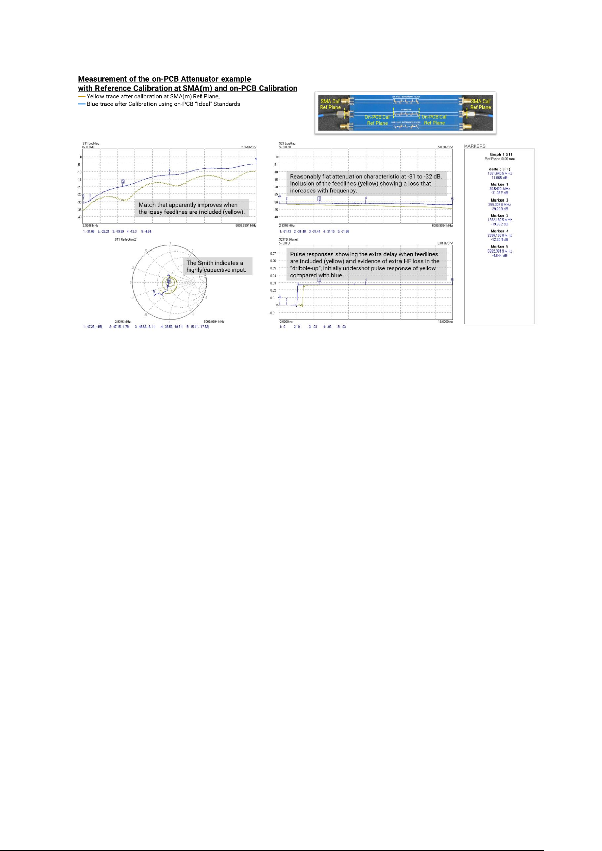
8.3 Measuring the on-PCB Attenuator example

Having calibrated at the SMA(m) test ports, connect to the on-PCB Attenuator example network.

From the recommended default settings, adjust to display instead:

• Display Ch2 – S21 Log Mag, 5.0 dB/div, Ref 0 U at grat 1.

• Display Ch3 – S11 Smith.

• Display Ch4 – S21 TD (Hann), 0.01 U/div, Ref 0 ns at grat 9, timebase –2 ns to 18 ns

• PicoVNA settings file: NMT kit Atten set.sta

In the screen shot below this measurement has been saved to Memory (yellow trace). This measurement shows relative good but declining match with increased frequency. Increased

delay; several rotations of the Smith chart, when feedline phase slip is included. And evidence of

increased HF loss in the “dribble-up” of the initially undershot pulse response of the yellow trace.

Network Metrology Traning Kit User’s Guide

Compare that with the blue trace that uses the on-PCB calibration. This shows the attenuator network itself to have reasonably flat frequency response at –31 to –32 dB; and quite highly capacitive input mismatch at HF. This had been somewhat hidden by the relative high HF loss of the feedline in the yellow trace.

Hint: Note again the ripple in the yellow S11 trace above. This is likely to result from multiple reflection in the 50 mm feedlines between the SMA / launch mismatch and that of the attenuator network.

Hint: Try touching the network and feedlines to cause additional mismatch at various points along the feedlines and attenuator sections, to see the range of impacts that can result.

Hint: Appendix 1 gives the schematic of the NMT kit PCA. Adjusted or alternative attenuators can be built and tested.

8.4 Measuring the on-PCB Bandpass Butterworth Filter example

Having calibrated at the SMA(m) test ports, connect the on-PCB Bandpass Filter example network.

From the recommended default settings, adjust to display instead:

• Display Ch3 – S11 Smith.

• Display Ch4 – S21, Group Delay, 5.0 ns/div, Ref 0 ns at grat 9.

• PicoVNA settings file: NMT kit BP Filter Wide set.sta

The measurement below reveals the filter to have a passband insertion loss of around –5 dB for frequencies between 150 and 250 MHz. It is fully reflective in its stop bands and it has relatively large group delay in its passband; with peaks at both roll points.

Network Metrology Traning Kit User’s Guide

To take a closer look apply a narrower sweep span around the passband. The measurement below uses 10 MHz to 610 MHz, 201 pts. The change to this new span will require either a new calibration for this span or an interpolation of the existing calibration. The latter interpolation feature is available on PicoVNA and on most other VNAs and is perfectly acceptable here.

In the screen shot below this measurement has been saved to Memory (yellow trace). It reveals more detail around the passband. If instead an on-PCB calibration is used, the blue trace results.

Group delay in particular is now seen as both substantial and it varies across the pass band, certainly at the band edges. Slight separation of the yellow and blue traces reveals the additional delay of the two feedlines (yellow). The same delay (2x Port 1 feedline) appears as an extra rotation on the Smith Chart.

Network Metrology Traning Kit User’s Guide

Please note that the PicoVNA Time Domain functionality does not support AC-coupled networks such as this bandpass network. The result on a time domain display will not be valid.

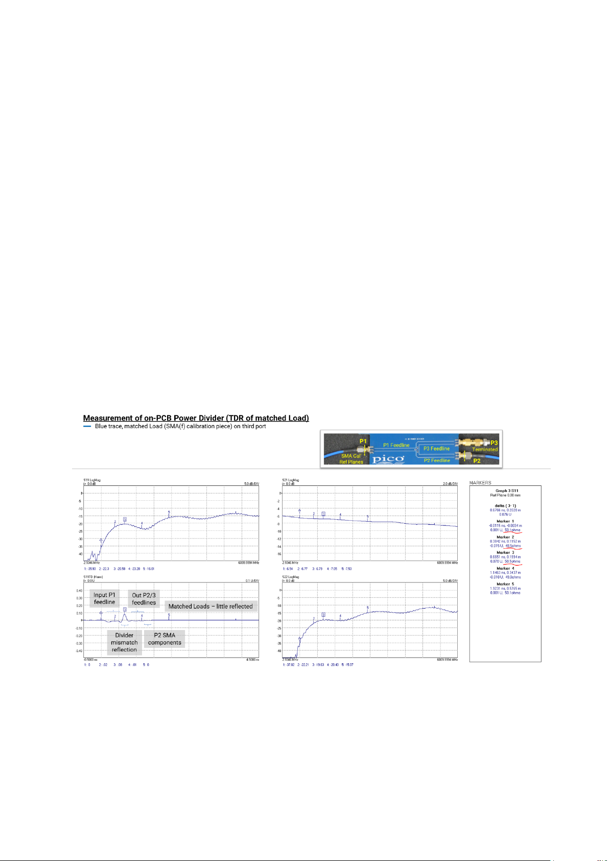
8.5 Measuring the on-PCB –6 dB Power Divider (time domain reflection) example

Having calibrated at the SMA(m) test ports, connect to the on-PCB –6 dB Power Divider example network. Connect Port 2 to the lower of the two right-hand ports. Terminate the upper of these ports with a matched load. The NMT kit contains a within series SMA(m-m) adaptor to facilitate use of SMA(f) Calibration Load as this terminator.

From the recommended default settings, adjust to display instead:

• Display Ch2 – S21 Log Mag, 2.0 dB/div, Ref 0 dB at grat 2

• Display Ch3 – S11 TD (Hann), 0.1 U/div, Ref 0 U at grat 6, timebase span –0.5 ns to

4.5 ns.

• PicoVNA settings file: NMT kit power divider set.sta

With the third port matched the two measured ports have good match that declines at HF. The transmission between measured ports is –6 dB with an additional loss that rises with frequency (the on-PCB feedlines are included in this measurement). When matched, the divider network (three 16.7 Ω resistors in a star arrangement) delivers one quarter (–6 dB) of the input power to each of the other ports, and dissipates the other half. Relating time to distance through the network, the time domain plot shows most of the higher frequency mismatch to be right at the divider network in the middle of the transmission path. Note the impedance measurements at each marker.

In the screen shot below the above measurement has been saved to Memory (yellow trace). This new measurement then shows the impact of mismatch, the SMA(f) calibration open at the third port. The Port 1 mismatch jumps to –12 dB (the forward and reverse loss of the divider). Mismatch at Port 1 and 2 look very similar and the time-domain plot shows an in-phase reflected step from a slightly longer SMA component path.

Network Metrology Traning Kit User’s Guide

Hint: Note that removal of the two SMA components will give another open, but right at the SMA launch connector. Try it.

Hint: With a –6 dB divider between P1 and the fully reflective mismatch on P3, we see a –12 dB match at P1. Given the matched condition on P2, in fact a –6 dB attenuator or “pad” would achieve exactly the same “improvement” in match as did the divider. The “padding” of mismatch is an often used principle in gigabit and microwave systems.

The measurement below saves the above plot from the SMA calibration open to the yellow trace and then fits the calibration short instead.

Network Metrology Traning Kit User’s Guide

Reflection phase reverses as evidenced in the port match and time domain plots. The time domain plot reveals the slightly shorter electrical length of the short (11.3 mm) compared with the open (13.0 mm).

If the yellow trace indicates high impedance, the blue trace low impedance and a flat trace indicates the matched (Z0 = 50 Ω) condition it is reasonable to conclude that every impedance is represented in the space between the traces. If we know propagation velocity, the time based x-axis also represents physical distance along the network path. Thus the time domain plot shows impedance transitions at physical locations along a network.

Note that in all the plots above, the impedance measurements at Markers 4 and 5 do not account the power divider loss and are therefore not accurate measures of line impedance at those points.

Hint: How well-matched are the divider ports? The above connections can be rotated to find out.

Hint: To see the effect of various other mismatches on P3, use a short coaxial cable to connect P3 to any of the other on-PCB networks. Remember to terminate the remaining network port correctly.

Hint: The power divider is used in time domain network analyzers as an alternative to the directional coupler that is used in the VNA. Whereas the VNA applies a sweep of individual frequencies to a network under test, the time-domain analyzer applies a spectrum of frequencies contained in a fast transition step, impulse or PRBS pattern, and observes responses on a broadband oscilloscope. The responses are exactly the same pulse or step responses that we see above.

If a fast step pulse source is available to drive P1 (e.g. transition time of 500 ps or faster) along with an oscilloscope of bandwidth 1 GHz or faster for P2 this can be demonstrated.

A PicoScope 9311 can demonstrate this stand-alone. Alternatively any PicoScope 9300 or 9400 with Pulse Generator PG900 can be used.

Network Metrology Traning Kit User’s Guide

8.6 Measuring the on-PCB 0603 surface mount component location.

To measure a component, the calibration reference plane needs to right at the component pads, requiring either an on-PCB calibration or a compensating characterization of the on-PCB feedlines (de-embed or ref-plane shift and normalization). Connect Port 1 to the Chip Component feedline. This will be a single port reflectometry measurement only, so Port 2 is not connected.

From the recommended default settings, adjust to display instead:

• Display Ch2 – S11 Smith Chart

• Display Ch3 – S11 TD (Hann), 0.25 U/div, Ref 0 U at grat 6, timebase span –1.0 ns to 9.0

ns.

• Display Ch4 – S11 Phase, 45°/div, Ref 0° at grat 6.

• PicoVNA settings file: NMT kit component set.sta

In this example a 3.3 pF 0603 capacitor has been soldered to the open pads provided.

Reference to the left-hand plots alone might lead to a contradiction. The time-domain plot indicates a short presented to high frequencies that transitions to an open in the long term (low frequencies). But the S11 plot indicates a constant magnitude of full reflection. This is not an impedance that passes anywhere close to 50 Ω in its transition between short and open.

The Smith Chart of course reveals what is going on: the component measures close to constant shunt capacitance rotating around the chart, a little lossy with increasing frequency and greater deviation beyond Marker 5. The chart enters the inductive region of the chart and wrapped phase flips on the phase plot.

The marker readouts give us a capacitance value that varies a little with frequency, more strongly at higher frequencies. This is because measurement sensitivity and therefore accuracy fall away as the measured impedance deviates from Z0 towards short or open. Best measurement will be at Mkr 2 and particularly if that is moved to slightly lower frequency, closer to the –90° phase point.

Network Metrology Traning Kit User’s Guide

The example below represents a 15.0 nH 0603 inductor soldered to the open pads.

Here is the opposing contradiction in the left-hand plots. The time-domain plot indicates an open presented to high frequencies that transitions to a short in the long term (low frequencies). Again the S11 plot indicates a constant reflection and no passing anywhere close to 50 Ω.

The Smith Chart again reveals what is going on: the component measures close to constant shunt inductance rotating around the chart, a little lossy with increasing frequency and greater deviation beyond Marker 5. The chart enters the capacitive region of the chart and wrapped phase flips on the phase plot.

The marker readouts give us a inductance value that varies a little with frequency, more strongly at higher frequencies. This is because measurement sensitivity and therefore accuracy fall away as the measured impedance deviates from Z0 towards short or open. Best measurement will be at Mkr 2 and particularly if that is moved to slightly higher frequency, closer to the –90° phase point.

In both cases significantly smaller values can be characterized in this way. Significantly larger values might require narrower sweeps to a reduced maximum frequency.

Note that with care, 0804 and 0402 surface mount components can also be accommodated on the solder pads provided.

8.7 Measuring the on-PCB broadband amplifier example

To measure the broadband amplifier, the calibration reference plane is best placed right at the input and output pads, requiring either an on-PCB calibration or a compensating characterization of the on-PCB feedlines (de-embed or ref-plane shift and normalization). There is also a need to provide an external + 5 V DC supply through the 2.1 mm connector. Current draw will be around 50 mA.

From the recommended default settings, adjust to display instead:

• Display Ch1 – S11 Log Mag, 2.0 dB/div, Ref 0 at grat 2.

• Display Ch2 – S21 Log Mag, 5.0 dB/div, Ref 0 at grat 5.

Network Metrology Traning Kit User’s Guide

• Display Ch3 – S12 Log Mag, 5.0 dB/div, Ref 0 at grat 5.

• Display Ch4 – S22 Log Mag, 2.0 dB/div, Ref 0 at grat 2.

For reasons that will become apparent two other setup changes:

1. Set the Port test level to –6 dBm

2. Replace the test lead on Port 2 with the SMA(m-m) adaptor**

The sweep span is also set to 2001 pts rather than the time-domain-compatible 2048 pts.

• PicoVNA settings file: NMT kit amplifier s-params set.sta

Perform a non-insertable calibration of this new setup using the on-PCB calibration standards and with their Ideal SOLT.kit data file loaded to both ports.

** Take care when aligning and connecting the training PCB to the now rigid test port on VNA Port 2. Support the PCB as shown throughout the measurements.

This particular calibration is used again in later sections so saving the calibration is recommended.

All the measurements that have been addressed above have been of passive, linear and reciprocal networks, for which it could have been seen that S21 and S12 were identical. Here for the first time the measurement is of an active non-reciprocal network: one in which forward transmission (or gain) S21 and reverse transmission (or isolation) S12 are very different. In this case, a signal incident at the DUT output is much attenuated at the DUT input port, while of course the forward path sees gain.

The measurement below shows a gain of +14.4 dB (~ x5) that begins to fall away –2.3 dB at 6 GHz and also at LF below around 30 MHz. This amplifier is AC-coupled.

Network Metrology Traning Kit User’s Guide

Changing the measurement view:

• Display Ch3 – S21 Phase, 45°/div, Ref 0° at grat 6.

• Display Ch4 – S21 Polar Linear, 1.25 U/div.

• PicoVNA settings file: NMT kit amplifier forward set.sta

This view shows forward transmission phase and linear–polar plots. Both confirm, from the lowfrequency characteristics, that this is an inverting amplifier and the linear–polar plot perhaps shows the low-frequency roll off more clearly.

Hint: It may be instructive to measure the amplifier with and without power applied.

Network Metrology Traning Kit User’s Guide

Unlike all previously described measurements, here the port power was reduced from –3 dBm to –6 dBm. All the other measurements have been performed on linear passive networks for which port power is irrelevant (assuming that it is not damaging or destructive to the DUT and not so low that measurement detail becomes lost in the measurement noise floor). In this case, with an active and possibly nonlinear network, port power may become relevant. To evaluate the potential impact of signal level the s-parameter measurements should be performed at various port power levels.

CAUTION – The additional consideration here is that due to the gain of the amplifier (up to +15 dB) the output power delivered to Port 2 of the VNA may become too large and may overload or even damage the Port 2 receivers. In the case of the PicoVNA 106 (depending upon sweep span) the port output power could approach +6 dBm and maximum saturating output power of the amplifier could approach +18 dBm. This will overload but will not damage the port. Note that the PicoVNA 2 user interface software issues a “beep” audible alarm when either port is overloaded and measurements may have become inaccurate.

To avoid the potential port receiver overload a –6 dB attenuator should be fitted to the amplifier output for a swept power measurement. It is convenient to use the –6 dB power divider network to achieve this, as shown in the setup below.

Do not forget to terminate the unused power divider port as shown!

Naturally, the measurement needs to be corrected to remove the –6 dB attenuator and any other interconnect mismatches, phase delays and losses from the measurement. An obvious approach is to measure and de-embed the inserted components. An alternative is to calibrate the measurement with the inserted lines and components included as elements of the test lead. Both of these correction approaches and their limitations will be described in sections 8.7.1 and 8.7.2 below.

Assuming one of the above correction methods is used, the plot below is an overlay of the same s-parameters measurement performed at eight different input levels and using the above test setup.

Network Metrology Traning Kit User’s Guide

Note that the multiple trace display such as above is on most VNAs limited by the number of available traces in each display channel. The illustrative image below is achieved using the PicoVNA and an overlay of partially transparent screen shot images.

The addition of the attenuator will desensitize measurements (reduce dynamic range) by –6 dB for transmission measurements, and by –12 dB for reflection measurements, on Port 2; but both of these compromises are tolerable in this measurement.

8.7.1 Measuring the on-PCB broadband amplifier example – measure and de-embed the “insertable”

output attenuator.

The image below shows the additional transmission lines and components that are inserted or embedded within the measurement. The network has a male SMA(m) input and female SMA(f)

output. This is known as an insertable network. To measure this network accurately we ideally need insertable test ports, one female and one male. Female and male test ports can of course be connected directly together and can then be disconnected to accept a so-called insertable network or component without adaptation. This is not true of our two ports of the same gender: the so-called non-insertable case.

Network Metrology Traning Kit User’s Guide

To perform this measurement we have to fit an SMA(f-f) adaptor to the male input port of the insertable network. That will add a little delay, loss and new mismatch errors, so we must perform the measurement in three parts:

1. Measure the SMA(f-f) adaptor

2. Measure the SMA(m-f) -6dB network with the SMA(f-f) adaptor fitted to the male port.

3. De-embed the SMA(f-f) adaptor from the measurement at Port 1

Before attempting any of this we must first calibrate at the SMA(m) test ports using in-kit SMA(f) SOLT calibration kit.

Note that the NMT kit SMA(f) Typ SOLT Vx.kit data must first be loaded to both ports for this calibration.

Network Metrology Traning Kit User’s Guide

Use the PicoVNA settings file: NMT kit amplifier s-params set.sta for this calibration and measurement.

Adjust the measurement view:

• Display Ch1 – S11 Log Mag, 5.0 dB/div, Ref 0 at grat 2.

• Display Ch4 – S22 Log Mag, 5.0 dB/div, Ref 0 at grat 2.

Firstly measure the SMA(f-f) and save this measurement as full .s2p Touchstone. A typical result is seen as the yellow measurement below.

Then disconnect the SMA(f-f) adaptor from Port 2 and connect as shown below to measure the two elements together. A typical result is seen as the blue measurement below.

Adjust the measurement view:

• Display Ch2 – S21 Log Mag, 1 dB/div, Ref 0 at grat 1

• Display Ch3 – S21 Phase, 45°/div, Ref 0° at grat 6.

Load the SMA(f-f) adaptor Touchstone file as the de-embed network on Port 1 and select deembed. The trace corrects slightly as the SMA(f-f) losses and delays are removed. Before (yellow trace) after de-embed (blue trace).

Network Metrology Traning Kit User’s Guide

Hint: There are several discussion points here. Why do all these measurement changes (and nonchange) occur as they do?

Save this new result as the Touchstone measurement of the –6 dB network that we wish to deembed from our main measurement. PicoVNA users should also save S21 as Log Magnitude + Phase text file as this will be needed for the P1dB utility as described in Section 8.8. This latter file needs a reduced number of sweep points, so before saving the file, adjust sweep points count to 201 pts and accept the use of an interpolated calibration. Re-start measurement and then save S21 as a Log Magnitude + Phase text file.

Hint: Note that the S21 phase plot very likely changes appearance with the reduction of sweep points. The displayed phase wrap points may shift slightly and the sawtooth tips may vary in amplitude. The measurements remain accurate but a deceptive alias of the wrapped phase waveform detail is probable against the reduction of measurement points. Be aware of this possibility when selecting the number of sweep points in your measurement.

Note that there is a potential for the above alias not to occur if the VNA in use is interpolating its measurements onto a higher available display resolution.

Return now to the calibration and measurement described in Section 7 above, i.e. the VNA ports calibrated using the on-PCB calibration standards and their Ideal SOLT.kit data (as below).

Network Metrology Traning Kit User’s Guide

Load the Touchstone result for the –6 dB embedded network to Port 2 and select de-embed to make the (blue trace) measurement shown below. Also load and display the previously stored and more directly made reference measurement for the amplifier (yellow trace) for the comparison below.

Hint: It may be instructive to toggle de-embed on off to see its substantial impact on all live plots.

The de-embed network is physically quite long (22 phase wraps to 6 GHz) and has a substantial –6 dB loss that will desensitize the S22 measurement by at least –12 dB. This, and the use of relatively poor calibration standards in the measurement of the de-embed network, lead to the larger error in Port 2 reflection. Nevertheless we have physically embedded and then successfully

Network Metrology Traning Kit User’s Guide

measured and mathematically de-embedded a substantial (length and loss) interfacing network.

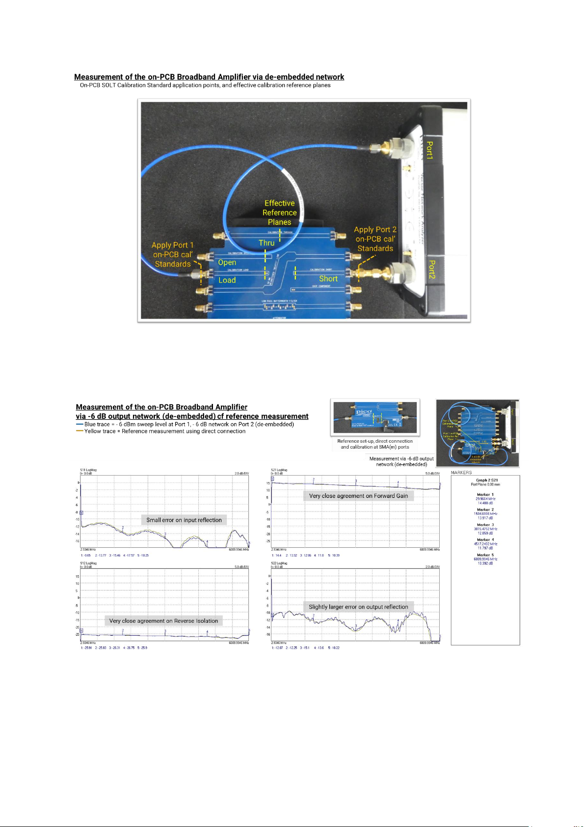
8.7.2 Measuring the on-PCB broadband amplifier example – calibrate to include an output attenuator

as part of the test feed.

An alternative measurement correction is to consider the embedded network as an integral part of the Port 2 test lead and to simply recalibrate the measurement with the network fitted within the Port 2 test lead.

We could choose to calibrate at the SMA(m) test ports by fitting the SMA(f) SOLT standards at the two SMA(m) test ports. However, the amplifier measurement that we require has its calibration reference planes at the on-PCB amplifier ports. So instead we should use the on-PCB SOLT standards and their Ideal SOLT.kit data, fitting them at the SMA(m) test ports but creating on-PCB virtual calibration reference planes as shown.

Use the PicoVNA settings file: NMT kit amplifier s-params set.sta for this calibration and measurement.

Network Metrology Traning Kit User’s Guide

Again, the embedded network is physically quite long (21 phase wraps to 6 GHz) and has a substantial –6 dB loss that will desensitize the S22 measurement by at least –12 dB; hence the larger error in Port 2 reflection. Nevertheless we have physically embedded and then successfully calibrated out a substantial interfacing network.

Having performed the calibration, reload the PicoVNA settings file NMT kit amplifier forward set.sta and remeasure the amplifier thus:

Both the de-embed and include-within-calibration techniques are compromised by small errors. The astute will observe that in the de-embed technique the embedded network does not quite sit at the Port 2 on-PCB calibration reference plane, but a little further back at SMA interface.

Network Metrology Traning Kit User’s Guide

The include-within-calibration method is subject to the errors of the “ideal” assumption for the on- PCB calibration standards in the presence of quite large corrections associated with the substantial network fitted on Port 2.

8.8 Measuring the non-linearity characteristic and the P1dB compression point of

the on-PCB amplifier

Section 8.7 demonstrated that the forward gain and phase of the power amplifier changes as the input power is increased, and that the change is not necessarily constant with frequency.

These are important non-linear network characteristics. Think for instance of a data communications symbol constellation and how vector amplitudes and phase might be corrupted by this amplifier.

Decode of these two constellations would survive the indicated degree of distortion, but for 256QAM or 1024QAM a reduced maximum output power would need to be tolerated.

Many VNAs, including the PicoVNA, can give us further visualization and measurement of the above gain compression and phase modulation due to amplitude modulation (PM due to AM, or AM to PM conversion).

Network Metrology Traning Kit User’s Guide

The plot to the right shows a typical compression characteristic. As input power increases, the output power deviates from the constant gain (dashed) characteristic with output power falling below expectation. The point at which output power is –1 dB below expectation is known as the P1dB point and is often a parameter of specification for amplifiers or signal outputs. P

SAT

, the saturated output power, may also be

specified.

To measure the P1dB point at a given frequency a VNA needs to sweep Port 1 power (the amplifier input power) and measure (amplifier output power) at Port 2. This is essentially an S21 measurement with stepping port powers, similar to that performed in Section 7, but at one defined frequency.

For those VNAs that do support this measurement, unfortunately test instruction will vary and a generic description cannot be given. However, key to an accurate measurement is that the insertion loss of the 6 dB network is accounted accurately somewhere. This might be achieved via the de-embedding described in Section 8.7.1, the inclusion within calibration described at Section 8.7.2 or, by entering an insertion loss for the network (at the specific test frequency).

For the PicoVNA, the latter method is described here.

The measurement and instrument settings are unchanged from that of Section 7, in which, to avoid overload of the VNA Port2 receivers, the –6 dB attenuating network is fitted to the amplifier output.

If required, reload the PicoVNA settings file NMT kit amplifier s-params set.sta

Calibrate as described at the beginning of Section 8.7, using the on-PCB SOLT to give on-PCB reference planes, at this point without account of the –6 dB output attenuation network.

The PicoVNA P1dB utility assumes a limited number of sweep points, so reduce this to 201 pts. Accept the use of interpolation to create a 201 pt calibration.

Network Metrology Traning Kit User’s Guide

Set 10 kHz resolution bandwidth and set Port Test Level to 3 dBm

Switch now to the P1dB gain compression utility. The graphical pop-up will display as shown below, initially without plots or data.

Select a frequency from the current span and then enter the corresponding loss of the –6 dB output network. This can be found by loading to memory trace or by inspecting (e.g. Windows Notepad) the de-embed Touchstone file that was saved and used in Section 8.7.1 (also as shown below).

Perform next the Calibrate, Start and Save steps to achieve something like this:

Network Metrology Traning Kit User’s Guide

8.9 Measuring level-dependent phase shift (AM to PM) of the on-PCB amplifier

Section 8.7 demonstrated that the forward gain and phase of the power amplifier changes as the input power is increased, and that the change is not necessarily constant with frequency. Focusing here on phase, the actual shift is very small for this particular amplifier and is barely noticeable in this multi-level plot (it can be seen with live traces or closer inspection).

However, the PicoVNA AM to PM utility (and equivalent functionality in some other VNAs) can extract small phase disturbances found at different amplifier output power levels.

Again, key to an accurate measurement is that the insertion loss of the –6 dB network is accounted accurately somewhere. This might be achieved via the de-embedding described in Section 8.7.1, the inclusion within calibration described at Section 8.7.2 or, by entering an insertion loss for the network (at the specific test frequency).

For the PicoVNA, the latter method is described.

The measurement and instrument settings are unchanged from those of Section 8.7, in which, to avoid overload of the VNA Port2 receivers, the –6 dB attenuating network is fitted to the amplifier output.

If required reload the PicoVNA settings file NMT kit amplifier s-params set.sta

Calibrate as described at the beginning of Section 8.7, using the on-PCB SOLT to give on-PCB reference planes, at this point without account of the –6 dB output attenuation network.

The PicoVNA P1dB utility assumes a limited number of sweep points, so reduce this to 201 pts. Accept the use of interpolation to create a 201 pt calibration.

Set 10 kHz resolution bandwidth and set Port Test Level to 3 dBm

Switch now to the AM to PM utility. The graphical pop-up will display as shown below, initially without plots or data.

As with the P1dB measurement of Section 8.9, select a frequency from the current span and then enter the corresponding loss of the –6 dB output network. This can be found by loading to memory trace or by inspecting (e.g. Windows Notepad) the de-embed Touchstone file that was

Network Metrology Traning Kit User’s Guide

saved and used in Section 8.7.1 (also as shown below).

Perform next the Calibrate and Start steps to achieve the plots below. Once the measurement is performed the selected input power for the readout can be changed to update results.

8.10 The mismatched Beatty line example – verifying a calibration and

measurement setup

Having established in Section 8.7 two correcting mechanisms for the necessary inclusion of an interfacing network, it would be valuable to have an effective mechanism for verification of calibration accuracy.

It is often thought that remeasurement of the calibration standards immediately after a calibration is an adequate check. Unfortunately, it is far from adequate. In practice, to remeasure a load or a thru, neither of which reflects with any significance, verifies only that we can measure them accurately when no reflection is present. Likewise, to remeasure a short or an open verifies only that we can measure a reflection accurately when very little or no transmission occurs.

When we calibrate a VNA, the data gathered from the measurement of short, open, load and thru is in fact used to calibrate a very much larger space in which all measurements are accurate in the presence of the others. A verification should demand an accurate set of measurement results from a wide variety of potentially interfering conditions. The mismatched Beatty line offers both varying and substantial match and a varying transmission characteristic.

Using the connections and setup below we can perform a comparative verification of the measurement corrections established in Sections 8.7.1 and 8.7.2.

Return to PicoVNA settings file NMT kit Default set.sta

Network Metrology Traning Kit User’s Guide

Increase sensitivity on Ch3 and adjust Ch4 display:

• Display Ch3 – S11 TD (Hann), 0.08 U/div, Ref 0 U at grat 6, timebase span –0.1 ns to 0.9

ns.

• Display Ch4 – S11 Phase, 45°/div, Ref 0° at grat 6

There is good agreement here between the correction mechanisms with a little more ripple, suggesting residual (incompletely corrected) mismatch as being present on the de-embedded measurements. It is probable that the above highlighted error in physical location of the deembed network (it sits on the SMA(f) output from the amplifier, not directly on its on-PCB port) contributes to this ripple. However, other potential error contributors are present and this result may not replicate every time.

Network Metrology Traning Kit User’s Guide

Hint: It may be instructive to attempt to de-embed or inclusively calibrate out the Beatty line from a measurement of the –6 dB divider.

8.10.1Verifying a calibration and measurement setup in terms of absolute accuracy

Included within the optional PQ187 or PQ188 demonstrator kits, Pico’s TA431 non-insertable Verification Standard works on the same principle as the Beatty line above. These devices however are very much more stable in their characteristic than the on-PCB example and these devices (like the calibration standard provided in the kits) are supplied with fully traceable measured data.

If you own either of these kits, the whole exercise performed in Section 8.10 and 8.7.1 / 8.7.2 can be performed or repeated, and the results compared with the traceable data, to truly discover which method results in the greater absolute measurement accuracy. Be aware however that in this case the calibration and de-embed reference planes must all be at the SMA interfaces rather than on-PCB and the use of the supplied phase and gain stable test leads is highly recommended.

Further, the Verification Standard can be used to compare the accuracy of a calibration using the kit supplied SMA(f) SOLT calibration kit or the high-quality kit also provided within the Demonstrator Kits.

Hint: An instructive additional exercise is to discover whether a Beatty line can be de-embedded or calibrated out from another Beatty line. Also possible to a more limited extent if you own two NMT kits.

Network Metrology Traning Kit User’s Guide

Appendix 1 - NMT kit PCA schematic

The schematic below allows for adjustment and repair of the PCA as supplied.

Network Metrology Traning Kit User’s Guide

Appendix 2 - Create a .kit from Touchstone measurements of SOLT standards

For those using the PicoVNA it is possible to measure other short, open, load and thru devices and create your own .kit calibration file of the comma-separated text file format below.

The file comprises polynomial models for the short and open (assuming the load to be ideal and that the thru will be measured in an “Unknown Thru” calibration), OR 201 pt measured data for all four components. The models and the four data files are concatenated into a file of just over 800 lines length.

Data is presented in Z0 = 50 Ω, real and imaginary format set against frequency in MHz.

Single-port data for the load, open and short, and two-port data for the thru, are shown below.

Polynomial models can be edited and saved using the Calibration Kit editor under the PicoVNA Tools menu. The thru will be measured during calibration.

United Kingdom global headquarters

Pico Technology James House Colmworth Business Park St Neots Cambridgeshire PE19 8YP United Kingdom

+44 (0) 1480 396 395 sales@picotech.com

North America regional office

Pico Technology 320 N Glenwood Blvd Tyler TX 75702 United States

+1 800 591 2796 sales@picotech.com

Asia-Pacific regional office

Pico Technology Room 2252, 22/F, Centro 568 Hengfeng Road Zhabei District Shanghai 200070 PR China

+86 21 2226-5152 pico.asia-pacific@picotech.com

www.picotech.com

Pico Technology PQ187 User Guide

Specifications and Main Features

Frequently Asked Questions

User Manual

1 Overview

2 Kit contents

2.1 PQ186 Network Metrology Training Kit Contents

2.2 PQ187 Standard Demonstrator Kit Contents

2.3 PQ188 Precision Demonstrator Kit Contents

3 Preparation

3.1 Preparation to use the PQ186 Network Metrology Training Kit

3.2 Preparation to use the PQ187 or PQ188 Network Metrology Demonstrator Kits

4 VNA calibration

4.1 VNA Calibration using the PQ190 Low Cost SMA(f) Calibration Kit

4.2 VNA calibration using the PQ186 NMT KIT PCA on-PCB SOLT standards

4.4 To calibrate or compensate feedlines?

5 Applying reference plane shift to compensate feedline length.

6 Applying normalization to compensate feedline loss

8 Measuring the on-PCB example networks

8.1 Measuring the on-PCB Calibration Thru Example

8.2 Measuring the on-PCB Low Pass Butterworth Filter Example

8.3 Measuring the on-PCB Attenuator example

8.4 Measuring the on-PCB Bandpass Butterworth Filter example

8.5 Measuring the on-PCB –6 dB Power Divider (time domain reflection) example

8.6 Measuring the on-PCB 0603 surface mount component location.

8.7 Measuring the on-PCB broadband amplifier example

8.9 Measuring level-dependent phase shift (AM to PM) of the on-PCB amplifier

8.10.1Verifying a calibration and measurement setup in terms of absolute accuracy