Omega Products FDT-40 Installation Manual

1 YEAR

®

WARRANTY

User’s Guide

omega.com

e-mail: [e-mail]

For latest product manuals:

omegamanual.info

FDT-40 and FDT-40E Series

Transit Time Ultrasonic Flow Meter

OMEGAnet®Online Service Internet e-mail

omega.com [e-mail]

Servicing North America:

U.S.A.: Omega Engineering, Inc., One Omega Drive, P.O. Box 4047

ISO 9001 Certied Stamford, CT 06907-0047 USA

Toll Free: 1-800-826-6342 TEL: [phone]
FAX: [phone] e-mail: [e-mail]

Canada: 976 Bergar

Laval (Quebec), Canada H7L 5A1
Toll-Free: 1-800-826-6342 TEL: [phone]
FAX: [phone] e-mail: [e-mail]

For immediate technical or application assistance:

U.S.A. and Canada: Sales Service: 1-800-826-6342/1-800-TC-OMEGA

Customer Service: 1-800-622-2378/1-800-622-BEST
Engineering Service: 1-800-872-9436/1-800-USA-WHEN

Mexico: En Español: 001 [phone] FAX: [phone]

[e-mail] e-mail: [e-mail]

®

®

®

Servicing Europe:

Benelux: Managed by the United Kingdom Office

Toll-Free: 0800 099 3344 TEL: [phone]
FAX: [phone] e-mail: [e-mail]

Czech Republic: Frystatska 184

733 01 Karviná, Czech Republic
Toll-Free: 0800-1-66342 TEL: [phone]
FAX: [phone] e-mail: [e-mail]

France: Managed by the United Kingdom Office

Toll-Free: 0800 466 342 TEL: [phone]
FAX: [phone] e-mail: [e-mail]

Germany/Austria: Daimlerstrasse 26

D-75392 Deckenpfronn, Germany
Toll-Free: 0 800 6397678 TEL: [phone]
FAX: [phone] e-mail: [e-mail]

United Kingdom: OMEGA Engineering Ltd.

ISO 9001 Certied One Omega Drive, River Bend Technology Centre, Northbank

Irlam, Manchester M44 5BD England
Toll-Free: 0800-488-488 TEL: [phone]
FAX: [phone] e-mail: [e-mail]

It is the policy of OMEGA Engineering, Inc. to comply with all worldwide safety and EMC/EMI
regulations that apply. OMEGA is constantly pursuing certification of its products to the European New
Approach Directives. OMEGA will add the CE mark to every appropriate device upon certification.

The information contained in this document is believed to be correct, but OMEGA accepts no liability for any
errors it contains, and reserves the right to alter specifications without notice.
WARNING: These products are not designed for use in, and should not be used for, human applications.

TABLE OF CONTENTS

QUICKSTART OPERATING INSTRUCTIONS ...................................................................8

1 - Transducer Location ...........................................................................................................................8

2 - Electrical Connections ........................................................................................................................9

3 - Pipe Preparation and Transducer Mounting ......................................................................................9

4 - Startup ..............................................................................................................................................10

INTRODUCTION ..............................................................................................................11

General...................................................................................................................................................11

Application Versatility ...........................................................................................................................11

CE Compliance .......................................................................................................................................12

User Safety .............................................................................................................................................12

Data Integrity ........................................................................................................................................12

Product Identi cation ............................................................................................................................12

PART 1  TRANSMITTER INSTALLATION........................................................................13

Transducer Connections ........................................................................................................................14

Line Voltage AC Power Connections .....................................................................................................15

Low Voltage AC Power Connections ......................................................................................................15

DC Power Connections ..........................................................................................................................16

PART 2  TRANSDUCER INSTALLATION ........................................................................17

General...................................................................................................................................................17

Step 1 - Mounting Location ...................................................................................................................17

Step 2 - Transducer Spacing ..................................................................................................................19

Step 3 - Entering Pipe and Liquid Data .................................................................................................21

Step 4 - Transducer Mounting ...............................................................................................................22

V-Mount and W-Mount Installation ......................................................................................................23

FDT-41 through FDT-46/FDT-41-HT through FDT-46-HT Small Pipe Transducer Installation .............24

Mounting Transducers in Z-Mount Con guration ................................................................................26

Mounting Track Installation ..................................................................................................................28

PART 3  INPUTS/OUTPUTS ............................................................................................29

General...................................................................................................................................................29

4-20 mA Output .....................................................................................................................................29

Control Outputs  ow Only version].......................................................................................................30

Optional Totalizing Pulse Speci cations...............................................................................................32

Frequency Output [ ow only units] .......................................................................................................33

RS485 .....................................................................................................................................................35

Heat Flow for energy units only ............................................................................................................36

3

PART 4  STARTUP AND CONFIGURATION ....................................................................39

Before Starting the Instrument .............................................................................................................39

Instrument Startup ................................................................................................................................39

Keypad Programming ...........................................................................................................................40

Menu Structure ......................................................................................................................................41

BSC Menu -- Basic Menu.........................................................................................................................41

CH1 Menu -- Channel 1 Menu ................................................................................................................52

CH2 Menu -- Channel 2 Menu ................................................................................................................54

SEN Menu -- Sensor Menu ......................................................................................................................56

SEC Menu -- Security Menu ....................................................................................................................57

SER Menu -- Service Menu .....................................................................................................................58

DSP Menu -- Display Menu ....................................................................................................................62

PART 5  SOFTWARE UTILITY .........................................................................................64

Introduction ...........................................................................................................................................64

System Requirements ............................................................................................................................64

Installation.............................................................................................................................................64

Initialization ..........................................................................................................................................64

Basic Tab ................................................................................................................................................66

Flow Tab .................................................................................................................................................68

Filtering Tab ...........................................................................................................................................71

Output Tab .............................................................................................................................................73

Channel 1 - 4-20 mA Con guration .......................................................................................................73

Channel 2 - RTD Con guration [for energy units Only] ........................................................................75

Channel 2 - Control Output Con guration Flow Only ..........................................................................76

Setting Zero and Calibration .................................................................................................................79

Target Dbg Data Screen - De nitions ....................................................................................................82

Saving Meter Con guration on a PC .....................................................................................................83

Printing a Flow Meter Con guration Report ........................................................................................83

APPENDIX ........................................................................................................................84

Speci cations .........................................................................................................................................85

Menu Maps ............................................................................................................................................86

Communications Protocols ...................................................................................................................90

Protocol Implementation Conformance Statement (Normative) ........................................................96

Heating and Cooling Measurement ......................................................................................................98

FDT-40 Error Codes ..............................................................................................................................103

Control Drawings .................................................................................................................................104

Brad Harrison® Connector Option .......................................................................................................110

K-Factors Explained .............................................................................................................................111

Fluid Properties ...................................................................................................................................114

Symbol Explanations ...........................................................................................................................116

CE Compliance Drawings ....................................................................................................................116

4

FIGURES

Figure Q.1 - Transducer Mounting Con gurations .................................................................................8

Figure Q.2 - Transducer Connections ......................................................................................................9

Figure 1.1 - Ultrasound Transmission ...................................................................................................11

Figure 1.2 - FDT-40 Transmitter Dimensions .........................................................................................13

Figure 1.3 - Transducer Connections .....................................................................................................14

Figure 1.4 - AC Power Connections ........................................................................................................15

Figure 1.5 - 24 VAC Power Connections .................................................................................................15

Figure 1.6 - DC Power Connections .......................................................................................................16

Figure 2.1- Transducer Mounting Modes — FDT-47, FDT-48, and FDT-47-HT ......................................20

Figure 2.2 - Transducer Orientation — Horizontal Pipes......................................................................22

Figure 2.3 - Transducer Alignment Marks .............................................................................................23

Figure 2.4 - Application of Couplent .....................................................................................................23

Figure 2.5 - Transducer Positioning .......................................................................................................24

Figure 2.6 - Application of Acoustic Couplent — FDT-41 through FDT-46/FDT-41-HT through FDT-46-

HT Transducers ......................................................................................................................................25

Figure 2.7 - Data Display Screen ...........................................................................................................25

Figure 2.8 - Calibration Page 3 of 3 .......................................................................................................25

Figure 2.9 - Calibration Points Editor ....................................................................................................25

Figure 2.10 - Edit Calibration Points .....................................................................................................26

Figure 2.11 - Paper Template Alignment ..............................................................................................27

Figure 2.12 - Bisecting the Pipe Circumference ....................................................................................27

Figure 2.14 - Mounting Track Installation .............................................................................................28

Figure 2.13 - Z-Mount Transducer Placement .......................................................................................28

Figure 3.1 - Allowable Loop Resistance (DC Powered Units) ................................................................29

Figure 3.2 - 4-20 mA Output ..................................................................................................................30

Figure 3.3 - Switch Settings ...................................................................................................................30

Figure 3.4 - Typical Control Connections ..............................................................................................31

Figure 3.5 - Single Point Alarm Operation ............................................................................................31

Figure 3.6 - Energy version Totalizer Output Option ............................................................................32

Figure 3.7 - Frequency Output Switch Settings .....................................................................................33

Figure 3.8 - Frequency Output Waveform (Simulated Turbine) ...........................................................34

Figure 3.9 - Frequency Output Waveform (Square Wave) ....................................................................34

Figure 3.10 - RS485 Network Connections ............................................................................................35

Figure 3.12 - Surface Mount RTD Installation .......................................................................................36

Figure 3.11 - RTD Schematic ..................................................................................................................36

Figure 3.14 - Connecting RTDs ..............................................................................................................37

Figure 3.13 - Insertion Style RTD Installation .......................................................................................37

Figure 3.15 - Ultrasonic Energy - RTD Adapter Connections ................................................................38

Figure 4.1 - Keypad Interface.................................................................................................................40

5

Figure 5.1 - Data Display Screen ...........................................................................................................65

Figure 5.2 - Basic Tab .............................................................................................................................67

Figure 5.3 - Flow Tab ..............................................................................................................................69

Figure 5.4 - Filtering Tab ........................................................................................................................71

Figure 5.5 - Output Tab ..........................................................................................................................73

Figure 5.6 - Channel 2 Input (RTD) ........................................................................................................76

Figure 5.7 - Channel 2 Output Choices ..................................................................................................77

Figure 5.8 - Calibration Page 1 of 3 .......................................................................................................79

Figure 5.9 - Calibration Page 2 of 3 .......................................................................................................80

Figure 5.10 - Calibration Page 3 of 3 .....................................................................................................81

Figure A-2.1 - Menu Map -- 1 .................................................................................................................87

Figure A-2.2 - Menu Map -- 2 .................................................................................................................88

Figure A-2.3 - Menu Map -- 3 .................................................................................................................89

Figure A-4.1 - Output Con guration Screen .........................................................................................99

Figure A-4.2 - RTD Calibration (Step 1 of 2) ........................................................................................100

Figure A-4.3 - RTD Calibration (Step 2 of 2) ........................................................................................101

Figure A-6.1 - Control Drawing I.S. Barrier FDT-47 Transducers ........................................................104

Figure A-6.2 - Control Drawing I.S. Barrier FDT-47 Transducers Flexible Conduit .............................105

Figure A-6.3 - Control Drawing Ultrasonic Flow (Class 1, Div II) .........................................................106

Figure A-6.4 - Control Drawing (Class 1, Div II DC) .............................................................................107

Figure A-6.5 - FDT-40 (AC) Hazardous Area Installation ....................................................................108

Figure A-6.6 - FDT-40 (DC) Hazardous Area Installation ....................................................................109

Figure A-7.1 - Brad Harrison® Connections .........................................................................................110

Figure A-11.1 - CE Compliance Drawing For AC Powered Meters .......................................................122

Figure A-11.2 - CE Compliance Drawing For DC Powered Meters ......................................................123

6

TABLES

Table 2.1 - Piping Con guration and Transducer Positioning ..............................................................18

Table 2.2 - Transducer Mounting Modes — FDT-47, FDT-48, and FDT-47-HT ......................................19

Table 2.3 - Transducer Mounting Modes — FDT-41 through FDT-46 / FDT-41-HT through FDT-46-HT

................................................................................................................................................................20

Table 3.1 - Dip Switch Functions ............................................................................................................30

Table 4.1 - Speci c Heat Capacity Values for Water ..............................................................................47

Table 4.2 - Speci c Heat Capacity Values for Other Common Fluids ....................................................48

Table 4.3 - Speci c Heat Capacity Values for Ethylene Glycol/Water ...................................................48

Table 4.4 - Exponent Values ...................................................................................................................50

Table 4.5 - RTDs ......................................................................................................................................54

Table 4.6 - Sound Speed of Water ..........................................................................................................58

Table 4.7 - Sample Substitute Flow Readings .......................................................................................60

Table 5.1 - Transducer Frequencies .......................................................................................................67

Table A-3.1 - Available Data Formats ....................................................................................................90

Table A-3.2 - Flow Meter MODBUS Register Map for ‘Little-endian’ Word Order Master Devices .......91

Table A-3.3 - Flow Meter MODBUS Register Map for ‘Big-endian’ Word Order Master Devices ..........91

Table A-3.4 - MODBUS Coil Map ............................................................................................................91

Table A-3.5 - Flow Meter BACnet® Object Mappings .............................................................................92

Table A-3.6 - BACnet® Standard Objects ...............................................................................................95

Table A-4.1 - Heat Capacity of Water ..................................................................................................102

Table A-4.2 - Standard RTD Resistance Values ....................................................................................102

Table A-5.1 - Flow Meter Error Codes ..................................................................................................103

Table A-5.2 - Electrical Symbols ...........................................................................................................103

Table A-8.1 - Fluid Properties ..............................................................................................................115

Table A-10.1 - ANSI Pipe Data ..............................................................................................................117

Table A-10.2 - ANSI Pipe Data ..............................................................................................................118

Table A-10.3 - Tube Data .....................................................................................................................119

Table A-10.4 - Ductile Iron Pipe Data ..................................................................................................120

Table A-10.5 - Cast Iron Pipe Data .......................................................................................................121

7

QUICKSTART OPERATING INSTRUCTIONS

This manual contains detailed operating instructions for all aspects of the  ow metering instrument.
The following condensed instructions are provided to assist the operator in getting the instrument
started up and running as quickly as possible. This pertains to basic operation only. If speci c instrument
features are to be used or if the installer is unfamiliar with this type of instrument, refer to the appro­priate section in the manual for complete details.

NOTE: The following steps require information supplied by the meter itself so it will be necessary to supply power to the unit, at
least temporarily, to obtain setup information.

1  TRANSDUCER LOCATION

1) In general, select a mounting location on the piping system with a minimum of 10 pipe diameters
(10 × the pipe inside diameter) of straight pipe upstream and 5 straight diameters downstream.
See Table 2.1 for additional con gurations.

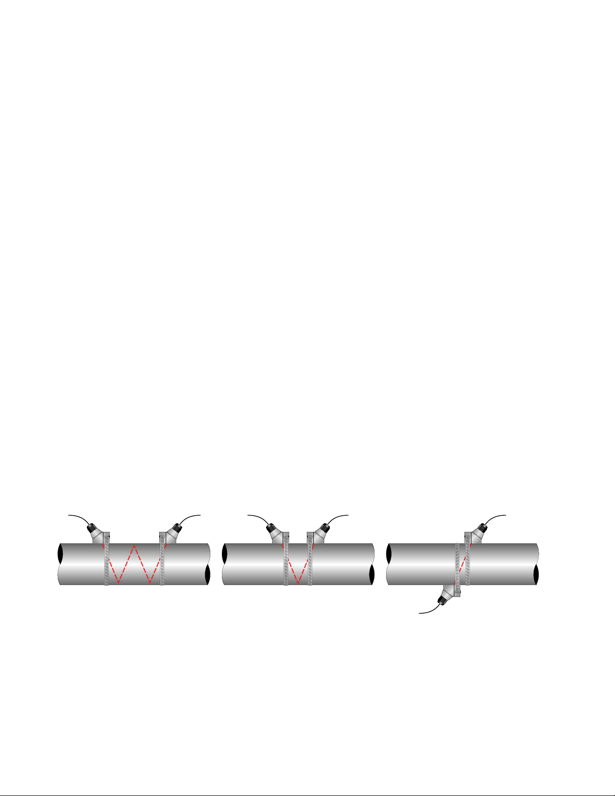
2) If the application requires FDT-47, FDT-48 or FDT-47-HT transducers select a mounting method for
the transducers based on pipe size and liquid characteristics. See Table 2.2. Transducer con gura-
tions are illustrated in Figure Q.1 below.

NOTE: All FDT-41 through FDT-46 and FDT-41-HT through FDT-46-HT transducers use V-Mount con guration.

3) Enter the following data into the transmitter via the integral keypad or the software utility:

1. Transducer mounting method 7. Pipe liner thickness

2. Pipe O.D. (Outside Diameter) 8. Pipe liner material

3. Pipe wall thickness 9. Fluid type

4. Pipe material 10. Fluid sound speed*

5. Pipe sound speed* 11. Fluid viscosity*

6. Pipe relative roughness* 12. Fluid speci c gravity*

* NOMINAL VALUES FOR THESE PARAMETERS ARE INCLUDED WITHIN THE FDT40 OPERATING SYSTEM. THE
NOMINAL VALUES MAY BE USED AS THEY APPEAR OR MAY BE MODIFIED IF THE EXACT SYSTEM VALUES ARE KNOWN.

TOP VIEW

OF PIPE

TOP VIEW

OF PIPE

TOP VIEW

OF PIPE

W-Mount V-Mount Z-Mount

FIGURE Q.1  TRANSDUCER MOUNTING CONFIGURATIONS

4) Record the value calculated and displayed as Transducer Spacing (XDC SPAC).

8

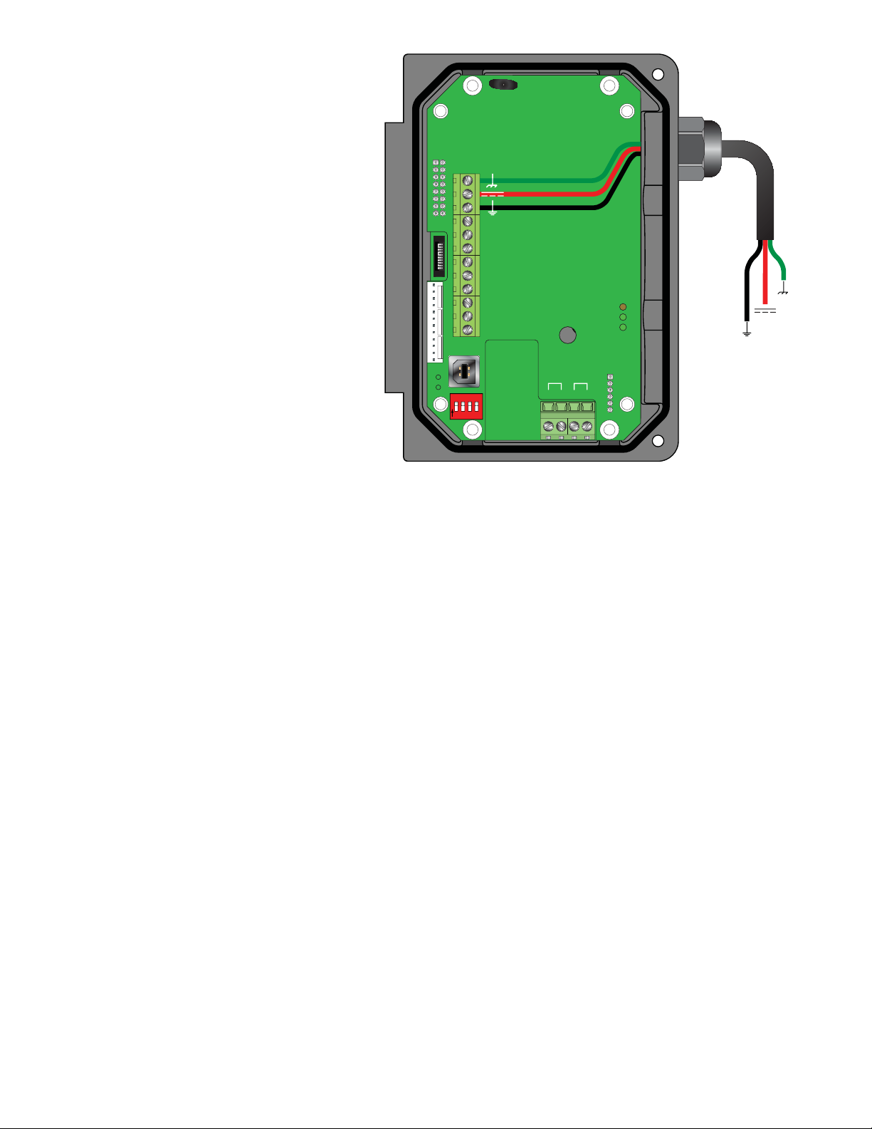
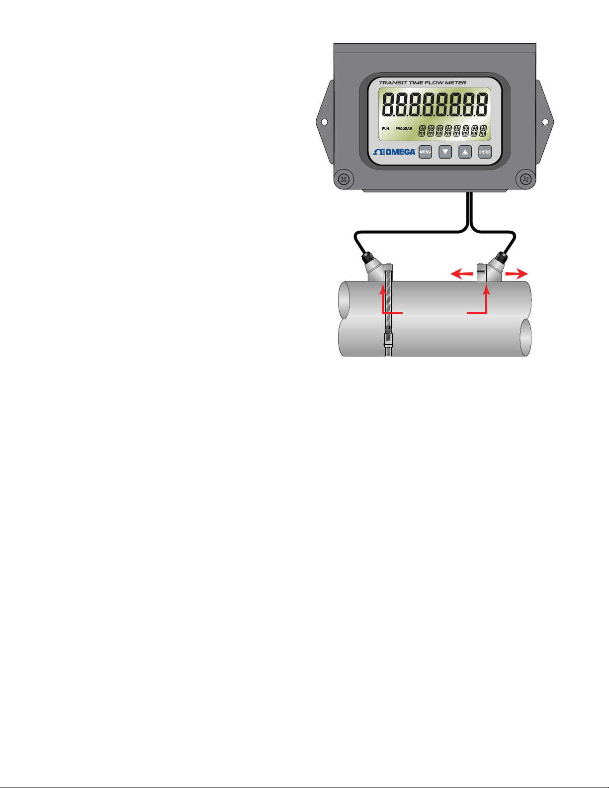
2  ELECTRICAL CONNECTIONS

TRANSDUCER/POWER CONNECTIONS

1) Route the transducer cables from the transducer mounting location back to the  ow meter
enclosure. Connect the transducer wires to the terminal block in the  ow meter enclosure.

2) Verify that power supply is correct for the meters

Downstream+
Downstream­Upstream­Upstream+

power option.

Line voltage AC units require 95 to 265 VAC
47 to 63 Hz @ 17 VA maximum.

Low voltage AC units require 20 to 28 VAC
47 to 63 Hz @ 0.35 A maximum.

FIGURE Q.2  TRANSDUCER CONNECTIONS

3) Connect power to the  ow meter.

DC units require 10 to 28 VDC @ 5 Watts maximum.

3  PIPE PREPARATION AND TRANSDUCER MOUNTING

(FDT-47, FDT-48, and FDT-47-HT Transducers)

1) Place the  ow meter in signal strength measuring mode. This value is available on the  ow meters
display (Service Menu) or in the data display of the software utility.

2) The pipe surface, where the transducers are to be mounted, must be clean and dry. Remove scale,
rust or loose paint to ensure satisfactory acoustic conduction. Wire brushing the rough surfaces
of pipes to smooth bare metal may also be useful. Plastic pipes do not require preparation other
than cleaning.

3) Apply a single ½” (12 mm) bead of acoustic couplent grease to the upstream transducer and
secure it to the pipe with a mounting strap.

4) Apply acoustic couplent grease to the downstream transducer and press it onto the pipe using
hand pressure at the lineal distance calculated in Step 1.

5) Space the transducers according to the recommended values found during programming or from
the software utility. Secure the transducers with the mounting straps at these locations.

9

(FDT-41 through FDT-46 and FDT-41-HT through FDT-46-HT Transducers)

1) Place the  ow meter in signal strength measuring mode. This value is available on the  ow
meter’s display (Service Menu) or in the data display of the software utility.

2) The pipe surface, where the transducers are to be mounted, must be clean and dry. Remove scale,
rust or loose paint to ensure satisfactory acoustic conduction. Wire brushing the rough surfaces
of pipes to smooth bare metal may also be useful. Plastic pipes do not require preparation other
than cleaning.

3) Apply a single ½” (12 mm) bead of acoustic couplent grease to the top half of the transducer and
secure it to the pipe with bottom half or U-bolts.

4) Tighten the nuts so that the acoustic coupling grease begins to  ow out from the edges of the
transducer and from the gap between the transducer and the pipe. Do not over tighten.

4  STARTUP

INITIAL SETTINGS AND POWER UP

1) Apply power to the transmitter.

2) Verify that SIG STR is greater than 5.0.

3) Input proper units of measure and I/O data.

10

INTRODUCTION

GENERAL

This transit time ultrasonic  ow meter is designed to measure the  uid velocity of liquid within a closed
conduit. The transducers are a non-contacting, clamp-on type or clamp-around, which will provide
bene ts of non-fouling operation
and ease of installation.

TOP VIEW

OF PIPE

TOP VIEW

OF PIPE

This family of transit time  ow
meters utilize two transducers
that function as both ultrasonic

W-Mount V-Mount Z-Mount

transmitters and receivers. The
transducers are clamped on the

FIGURE 1.1  ULTRASOUND TRANSMISSION

outside of a closed pipe at a speci c distance from each other. The transducers can be mounted in
V-Mount where the sound transverses the pipe two times, W-Mount where the sound transverses the

pipe four times, or in Z-Mount where the transducers are mounted on opposite sides of the pipe and the
sound crosses the pipe once. The selection of mounting method is based on pipe and liquid characteris­tics which both have an e ect on how much signal is generated. The  ow meter operates by alternately
transmitting and receiving a frequency modulated burst of sound energy between the two transducers
and measuring the time interval that it takes for sound to travel between the two transducers. The di er­ence in the time interval measured is directly related to the velocity of the liquid in the pipe.

TOP VIEW

OF PIPE

APPLICATION VERSATILITY

This  ow meter can be successfully applied on a wide range of metering applications. The simple-to­program transmitter allows the standard product to be used on pipe sizes ranging from ½ inch to 100
inches (12 mm to 2540 mm)*. A variety of liquid applications can be accommodated:

ultrapure liquids cooling water
potable water river water
chemicals plant e uent
sewage others
reclaimed water

Because the transducers are non-contacting and have no moving parts, the  ow meter is not a ected
by system pressure, fouling or wear. Standard transducers, FDT-47 and FDT-48 are rated to a pipe surface
temperature of -40 to +250 °F (-40 to +121 °C). FDT-41 through FDT-46 small pipe transducers are rated
from -40 to +185 °F (-40 to +85 °C). The FDT-47-HT high temperature transducers can operate to a pipe
surface temperature of -40 to +350 °F (-40 to +176 °C) and the FDT-41-HT through FDT-46-HT small pipe
high temperature transducer will withstand temperature of -40 to +250 °F (-40 to +121 °C).

*ALL ½” TO 1½” SMALL PIPE TRANSDUCERS AND 2” SMALL PIPE TUBING TRANSDUCER SETS REQUIRE THE TRANS
MITTER BE CONFIGURED FOR 2 MHz AND USE DEDICATED PIPE TRANSDUCERS. FDT48 TRANSDUCERS REQUIRE THE
USE OF THE 500 KH
THE SOFTWARE UTILITY OR THE TRANSMITTER’S KEYPAD.

Z TRANSMISSION FREQUENCY. THE TRANSMISSION FREQUENCY IS SELECTABLE USING EITHER

11

CE COMPLIANCE

The transmitter can be installed in conformance to CISPR 11 (EN 55011) standards. See the CE Compli­ance drawings in the Appendix of this manual.

USER SAFETY

This meter employs modular construction and provides electrical safety for the operator. The display
face contains voltages no greater than 28 VDC. The display face swings open to allow access to user
connections.

Danger: The power supply board can have line voltages applied to it, so disconnect electrical
power before opening the instrument enclosure. Wiring should always conform to local codes
and the National Electrical Code®.

DATA INTEGRITY

Non-volatile  ash memory retains all user-entered con guration values in memory for several years at
77 °F (25 °C), even if power is lost or turned o . Password protection is provided as part of the Security
menu (SEC MENU) and prevents inadvertent con guration changes or totalizer resets.

PRODUCT IDENTIFICATION

The serial number and complete model number of the transmitter are located on the top outside surface
of the transmitter’s body. Should technical assistance be required, please provide the Customer Service
Department with this information.

12

PART 1  TRANSMITTER INSTALLATION

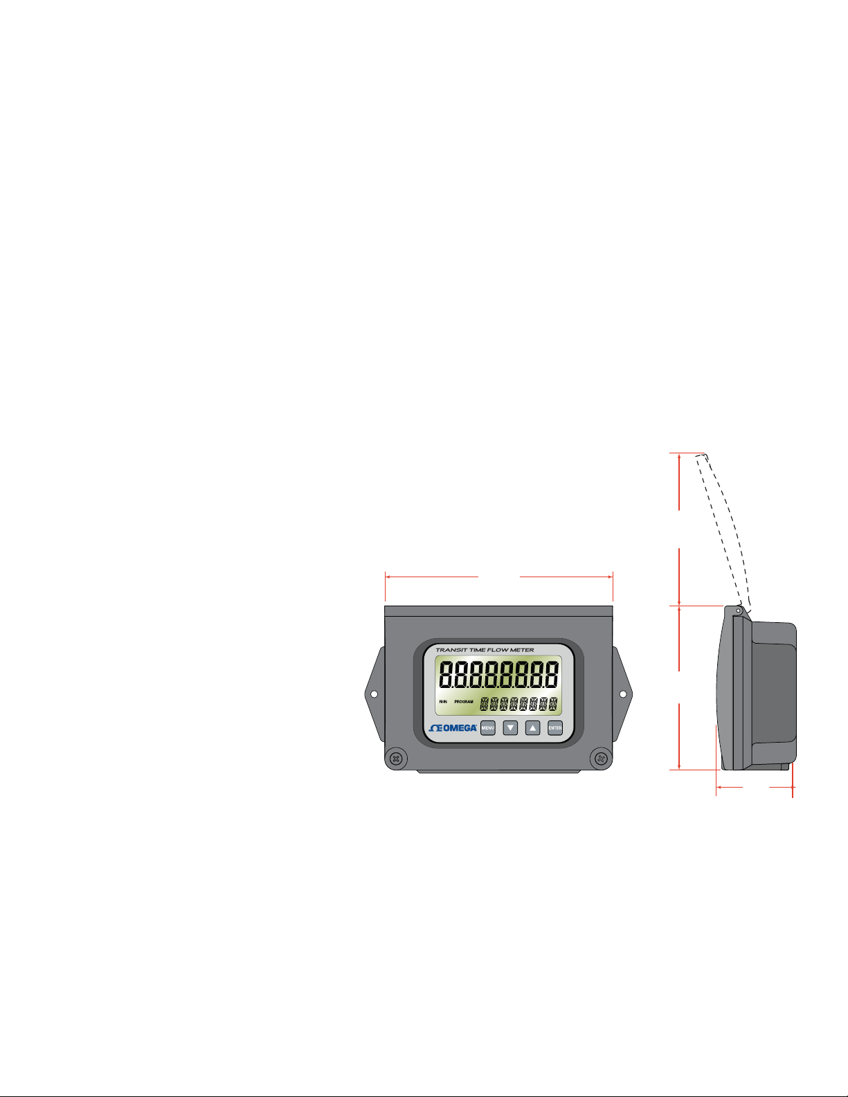
4.32

(109.7)

4.20

(106.7)

2.06

(52.3)

6.00

(152.4)

After unpacking, it is recommended to save the shipping carton and packing materials in case the instru­ment is stored or re-shipped. Inspect the equipment and carton for damage. If there is evidence of ship­ping damage, notify the carrier immediately.

The enclosure should be mounted in an area that is convenient for servicing, calibration or for observa­tion of the LCD readout.

1) Locate the transmitter within the length of transducer cables supplied. If this is not possible, it is
recommended that the cable be exchanged for one that is of proper length. To add cable length
to a transducer, the cable must be the same type as utilized on the transducer. Twinaxial cables
can be lengthened with like cable to a maximum overall length of 100 feet (30 meters). Coaxial
cables can be lengthened with RG59 75 Ohm cable and BNC connectors to 990 feet (300 meters).

2) Mount the transmitter in a location:

~ Where little vibration exists.

~

That is protected from corrosive  uids.

~ That is within the transmitters ambient temperature limits -40 to +185 °F (-40 to +85 °C).
~ That is out of direct sunlight. Direct sunlight may increase transmitter

temperature to above the maximum limit.

3) Mounting - Refer to Figure 1.2 for enclosure and mounting dimension
details. Ensure that enough room is available to allow for door swing, main­tenance and conduit entrances.
Secure the enclosure to a  at
surface with two appropriate
fasteners.

4) Conduit Holes - Conduit holes
should be used where cables
enter the enclosure. Holes not
used for cable entry should be
sealed with plugs.

An optional cable gland kit is
available for inserting trans­ducer and power cables. The
manufacturers part number for
this kit is FDT-40-Cable Gland
Kit and can be ordered directly
from the manufacturer.

NOTE: Use NEMA 4 [IP-65] rated  ttings/plugs to maintain the watertight integrity of the enclosure. Generally, the right conduit
hole (viewed from front) is used for power, the left conduit hole for transducer connections, and the center hole is utilized for I/O
wiring.

FIGURE 1.2  FDT40 TRANSMITTER DIMENSIONS

13

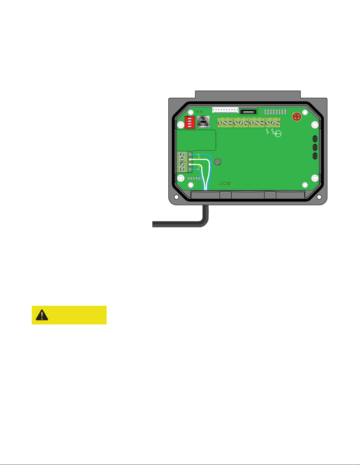
TRANSDUCER CONNECTIONS

To access terminal strips for wiring, loosen the two screws in the enclosure door and open.

Guide the transducer terminations through the transmitter conduit hole located in the bottom-left of
the enclosure. Secure the transducer cable with the supplied conduit nut (if  exible conduit was ordered
with the transducer).

The terminals within  ow meter are of a
screw-down barrier terminal type. Connect
the appropriate wires at the corresponding
screw terminals in the transmitter. Observe
upstream and downstream orientation
and wire polarity. See Figure 1.3.

O

N

1234

RS485 Gnd

RS485 A(-)

RS485 B(+)

Reset Total

4-20 mA Out

Frequency Out

Control 2

Control 1

Signal Gnd.

95 - 264 VAC

AC Neutral

372

VE
D

1500mA250V

C US

R

W

NOTE: Transducer cables have two possible wire
colors. For the blue and white combination the blue
wire is positive (+) and the white wire is negative (-).
For the red and black combination the red wire is

+

+

Downstream

Downstream

-

-

-

-

Upstream

Upstream

+

+

TFX Tx

Modbus

TFX Rx

positive (+) and the black wire is negative (-).

NOTE: The transducer cable carries low level, high
frequency signals. In general, it is not recommended
to add additional length to the cable supplied with
the transducers. Cables 100 to 990 feet (30 to 300

To Transducers

meters) are available with RG59 75 Ohm coaxial
cable. If additional cable is added, ensure that
it is the same type as utilized on the transducer.

FIGURE 1.3  TRANSDUCER CONNECTIONS

Twinaxial (blue and white conductor) cables can be
lengthened with like cable to a maximum overall length of 100 feet (30 meters). Coaxial cables can be lengthened with RG59
75 Ohm cable and BNC connectors to 990 feet (300 meters).

Connect power to the screw terminal block in the transmitter. See Figure 1.4 and Figure 1.5. Utilize the
conduit hole on the right side of the enclosure for this purpose. Use wiring practices that conform to
local and national codes (e.g., The National Electrical Code® Handbook in the U.S.)

CAUTION

CAUTION: Any other wiring method may be unsafe or cause improper operation of the instrument.

NOTE: This instrument requires clean electrical line power. Do not operate this unit on circuits with noisy components (i.e.,
 uorescent lights, relays, compressors, or variable frequency drives). The use of step down transformers from high voltage, high
amperage sources is also not recommended. Do not to run signal wires with line power within the same wiring tray or conduit.

14

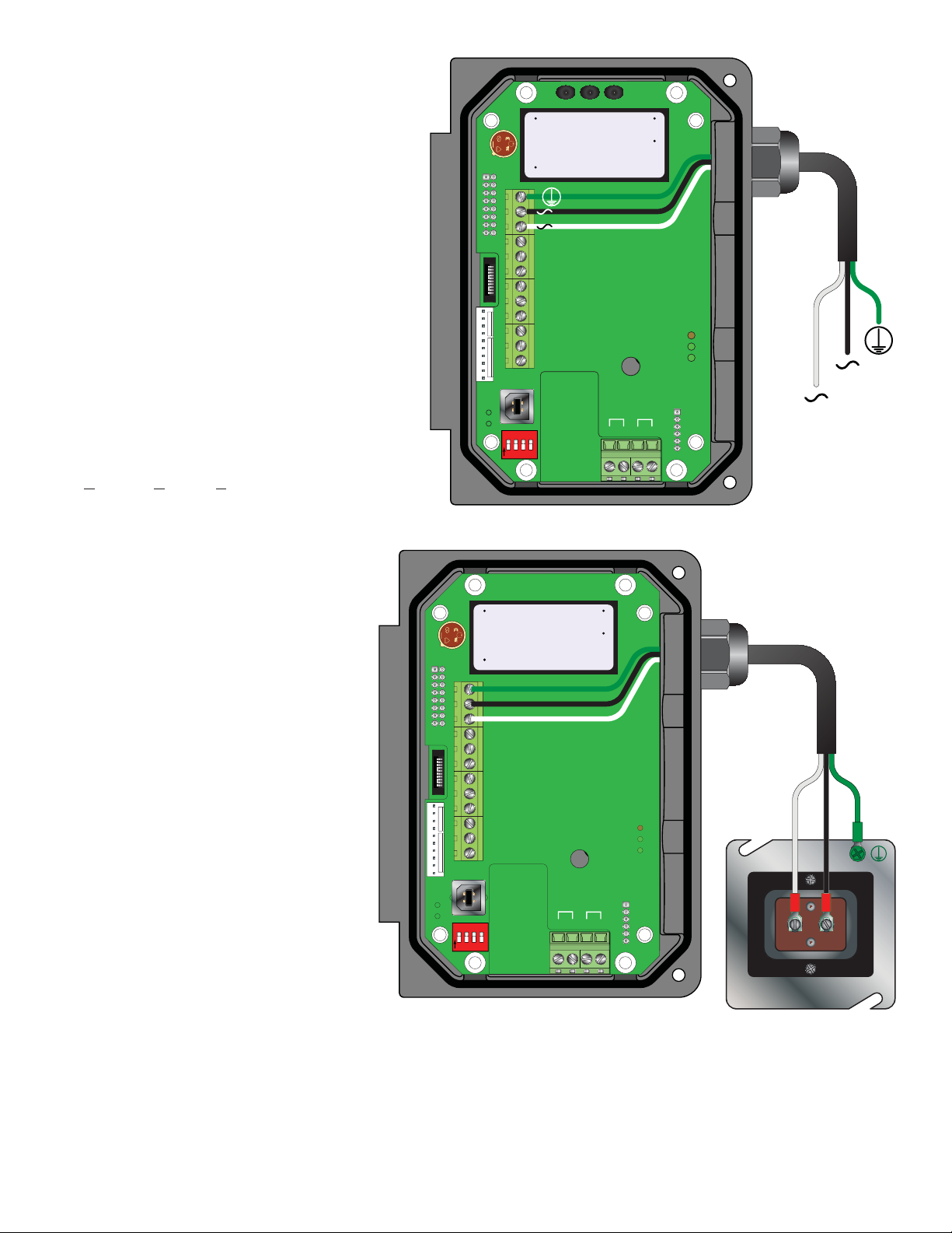
LINE VOLTAGE AC POWER
CONNECTIONS

Connect 90 to 265 VAC, AC Neutral and
Chassis Ground to the terminals referenced
in Figure 1.4. Do not operate without an
earth (chassis) ground connection.

LOW VOLTAGE AC POWER
CONNECTIONS

Connect 20 to 28 VAC, AC Neutral and
Chassis Ground to the terminals referenced
in Figure 1.5. Do not operate without an
earth (chassis) ground connection.

The 24 VAC power supply option for this
meter is intended for a typical HVAC and
Building Control Systems (BCS) powered
by a 24 VAC, nominal, power source. This
power source is provided by AC line power
to 24 VAC drop down transformer
and is installed by the installation
electricians.

NOTE: In electrically noisy applications,
grounding the meter to the pipe where
the transducers are mounted may provide
additional noise suppression. This approach
is only e ective with conductive metal
pipes. The earth (chassis) ground derived
from the line voltage power supply should
be removed at the meter and a new earth
ground connected between the meter and
the pipe being measured.

NOTE: Wire gauges up to 14 AWG can be
accommodated in the  ow meter terminal
blocks.

NOTE: AC powered versions are protected
by a  eld replaceable fuse. This fuse is
equivalent to Wickmann P.N. 3720500041 or

37405000410.

+Vo

-Vo

Modbus

TFX Rx
TFX Tx

Downstream

Upstream

-

-

+

+

372

VE

D

1500mA250V

W

C US

R

O

1234

N

ACN

ACL

95 - 264 VAC

95 - 264 VAC

AC Neutral

AC Neutral
Signal Gnd.
Control 1
Control 2
Frequency Out
4-20 mA Out
Reset Total
RS485 Gnd
RS485 A(-)
RS485 B(+)

FIGURE 1.4  AC POWER CONNECTIONS

ACN

1500mA250V

372

W

C US

VE

D

R

ACL

Chassis Gnd.
24 VAC
AC Neutral

Signal Gnd.
Control 1
Control 2
Frequency Out
4-20 mA Out
Reset Total
RS485 Gnd
RS485 A(-)
RS485 B(+)

Tes t

P1

O

1234

N

+Vo

-Vo

Modbus

TFX Rx
TFX Tx

Downstream

Upstream

-

-

+

+

24 VAC

Transformer

FIGURE 1.5  24 VAC POWER CONNECTIONS

15

DC POWER CONNECTIONS

The  ow meter may be operated from a 10
to 28 VDC source, as long as the source is
capable of supplying a minimum of 5 Watts
of power.

Connect the DC power to 10 to 28 VDC In,
Power Gnd., and Chassis Gnd., as in Figure

1.6.

NOTE: DC powered versions are protected by an

automatically resetting fuse. This fuse does not
require replacement.

O

1234

N

10 - 28 VDC

10 - 28 VDC

Power Gnd.

Power Gnd.
Signal Gnd.
Control 1
Control 2
Frequency Out
4-20 mA Out
Reset Total
RS485 Gnd
RS485 A(-)
RS485 B(+)

Modbus

TFX Rx
TFX Tx

Downstream

Upstream

-

-

+

+

Power

Ground

10 -28 VDC

FIGURE 1.6  DC POWER CONNECTIONS

16

PART 2  TRANSDUCER INSTALLATION

GENERAL

The transducers that are utilized by this  ow meter contain piezoelectric crystals for transmitting and
receiving ultrasonic signals through walls of liquid piping systems. FDT-47, FDT-48 and FDT-47-HT trans­ducers are relatively simple and straightforward to install, but spacing and alignment of the transducers
is critical to the system’s accuracy and performance. Extra care should be taken to ensure that these
instructions are carefully executed. FDT-41 through FDT-46 and FDT-41-HT through FDT-46-HT, small
pipe transducers, have integrated transmitter and receiver elements that eliminate the requirement for
spacing measurement and alignment.

Mounting of the FDT-47, FDT-48, and FDT-47-HT clamp-on ultrasonic transit time transducers is
comprised of three steps:

1) Selection of the optimum location on a piping system.

2) Entering the pipe and liquid parameters into either the software utility or keying the parameters
into transmitter using the keypad. The software utility or the transmitters  rmware will calculate
proper transducer spacing based on these entries.

3) Pipe preparation and transducer mounting.

Energy transmitters require two RTDs to measure heat usage. The  ow meter utilizes 1,000 Ohm, three­wire, platinum RTDs in two mounting styles. Surface mount RTDs are available for use on well insulated
pipes. If the area where the RTD will be located is not insulated, inconsistent temperature readings will
result and insertion (wetted) RTDs should be utilized.

STEP 1  MOUNTING LOCATION

The  rst step in the installation process is the selection of an optimum location for the  ow measure­ment to be made. For this to be done e ectively, a basic knowledge of the piping system and its
plumbing are required.

An optimum location is de ned as:

~ A piping system that is completely full of liquid when measurements are being taken. The pipe

may become completely empty during a process cycle – which will result in the error code 0010
(Low Signal Strength) being displayed on the  ow meter while the pipe is empty. This error code
will clear automatically once the pipe re lls with liquid. It is not recommended to mount the
transducers in an area where the pipe may become partially  lled. Partially  lled pipes will cause
erroneous and unpredictable operation of the meter.

~ A piping system that contains lengths of straight pipe such as those described in Table 2.1. The

optimum straight pipe diameter recommendations apply to pipes in both horizontal and vertical
orientation. The straight runs in Table 2.1 apply to liquid velocities that are nominally 7 FPS (2.2
MPS). As liquid velocity increases above this nominal rate, the requirement for straight pipe
increases proportionally.

~ Mount the transducers in an area where they will not be inadvertently bumped or disturbed

during normal operation.

~ Avoid installations on downward  owing pipes unless adequate downstream head pressure is

present to overcome partial  lling of or cavitation in the pipe.

17

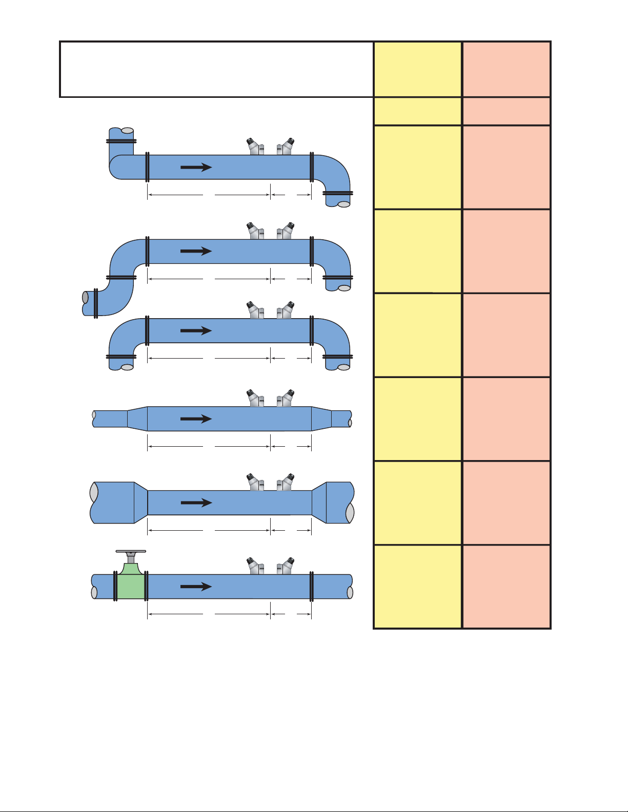
Piping Configuration

and Transducer Positioning

Upstream

Pipe

Diameters

Downstream

Pipe

Diameters

***

Flow

Flow

Flow

Flow

24

*

**

14

*

**

10

*

**

10

*

**

5

5

5

5

Flow

*

Flow

*

TABLE 2.1  PIPING CONFIGURATION AND TRANSDUCER POSITIONING

This  ow meter system will provide repeatable measurements on piping systems that do not meet these
requirements, but accuracy of these readings may be in uenced to various degrees.

18

**

**

10

24

5

5

STEP 2  TRANSDUCER SPACING

The transmitter can be used with  ve di erent transducer types: FDT-47, FDT-48, FDT-47-HT, FDT-41
through FDT-46 and FDT-41-HT through FDT-46-HT. Meters that utilize the FDT-47, FDT-48, or FDT­47-HT transducer sets consist of two separate sensors that function as both ultrasonic transmitters and
receivers. FDT-41 through FDT-46 and FDT-41-HT through FDT-46-HT transducers integrate both the
transmitter and receiver into one assembly that  xes the separation of the piezoelectric crystals. FDT-47,
FDT-48, and FDT-47-HT transducers are clamped on the outside of a closed pipe at a speci c distance
from each other.

The FDT-47, FDT-48, and FDT-47-HT transducers can be mounted in:

W-Mount where the sound traverses the pipe four times. This mounting method produces the
best relative travel time values but the weakest signal strength.
V-Mount where the sound traverses the pipe twice. V-Mount is a compromise between travel
time and signal strength.
Z-Mount where the transducers are mounted on opposite sides of the pipe and the sound crosses
the pipe once. Z-Mount will yield the best signal strength but the smallest relative travel time.

Transducer Mount Mode Pipe Material Pipe Size Liquid Composition

Plastic (all types)

W-Mount

V-Mount

Z-Mount

Carbon Steel

2-4 in. (50-100 mm)

Stainless Steel
Copper
Ductile Iron

Not recommended

Cast Iron
Plastic (all types)

4-12 in. (100-300 mm)Carbon Steel

Stainless Steel

Low TSS; non-aerated

Copper 4-30 in. (100-750 mm)
Ductile Iron

2-12 in. (50-300 mm)

Cast Iron
Plastic (all types) > 30 in. (> 750 mm)
Carbon Steel

> 12 in. (> 300 mm)

Stainless Steel
Copper > 30 in. (> 750 mm)
Ductile Iron

> 12 in. (> 300 mm)

Cast Iron

TSS = Total Suspended Solids

TABLE 2.2  TRANSDUCER MOUNTING MODES  FDT47, FDT48, AND FDT47HT

19

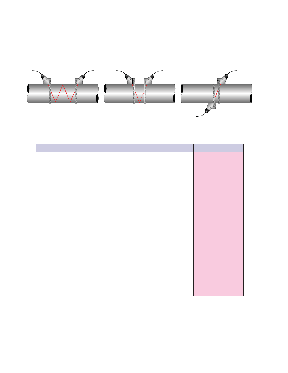
For further details, reference Figure 2.1. The appropriate mounting con guration is based on pipe and
liquid characteristics. Selection of the proper transducer mounting method is not entirely predictable
and many times is an iterative process. Table 2.2 contains recommended mounting con gurations for
common applications. These recommended con gurations may need to be modi ed for speci c appli­cations if such things as aeration, suspended solids, out of round piping or poor piping conditions are
present. Use of the  ow meter diagnostics in determining the optimum transducer mounting is covered
later in this section.

TOP VIEW

OF PIPE

TOP VIEW

OF PIPE

TOP VIEW

OF PIPE

W-Mount V-Mount Z-Mount

FIGURE 2.1 TRANSDUCER MOUNTING MODES  FDT47, FDT48, AND FDT47HT

Size Frequency Setting Transducer Mounting Mode

FDT-41-ANSI FDT-41-ANSI-HT

½ 2 MHz

¾ 2 MHz

1 2 MHz

FDT-41-CP FDT-41-CP-HT
FDT-41-T FDT-41-T-HT
FDT-42-ANSI FDT-42-ANSI-HT
FDT-42-CP FDT-42-CP-HT
FDT-42-T FDT-42-T-HT
FDT-43-ANSI FDT-43-ANSI-HT
FDT-43-CP FDT-43-CP-HT
FDT-43-T FDT-43-T-HT
FDT-44-ANSI FDT-44-ANSI-HT

V

1¼ 2 MHz

FDT-44-CP FDT-44-CP-HT
FDT-44-T FDT-44-T-HT
FDT-45-ANSI FDT-45-ANSI-HT

1½ 2 MHz

FDT-45-CP FDT-45-CP-HT
FDT-45-T FDT-45-T-HT
FDT-46-ANSI FDT-46-ANSI-HT

1 MHz

2

FDT-46-CP FDT-46-CP-HT

2 MHz FDT-46-T FDT-46-T-HT

TABLE 2.3  TRANSDUCER MOUNTING MODES  FDT41 THROUGH FDT46 / FDT41HT THROUGH

FDT46HT

For pipes 24” (600 mm) and larger the FDT-48 transducers using a transmission frequency of 500 KHz are
recommended.

20

FDT-48 transducers may also be advantageous on pipes between 4” and 24” if there are less quanti able
complicating aspects such as – sludge, tuberculation, scale, rubber liners, plastic liners, thick mortar, gas
bubbles, suspended solids, emulsions, or pipes that are perhaps partially buried where a V-mount is
required/desired, etc.

STEP 3  ENTERING PIPE AND LIQUID DATA

This metering system calculates proper transducer spacing by utilizing piping and liquid information
entered by the user. This information can be entered via the keypad on the  ow meter or via the optional
software utility.

The best accuracy is achieved when transducer spacing is exactly what the  ow meter calculates, so
the calculated spacing should be used if signal strength is satisfactory. If the pipe is not round, the wall
thickness not correct or the actual liquid being measured has a di erent sound speed than the liquid
programmed into the transmitter, the spacing can vary from the calculated value. If that is the case, the
transducers should be placed at the highest signal level observed by moving the transducers slowly
around the mount area.

NOTE: Transducer spacing is calculated on “ideal” pipe. Ideal pipe is almost never found so the transducer spacing distances may
need to be altered. An e ective way to maximize signal strength is to con gure the display to show signal strength,  x one trans­ducer on the pipe and then starting at the calculated spacing, move the remaining transducer small distances forward and back
to  nd the maximum signal strength point.

Important! Enter all of the data on this list, save the data and reset the  ow meter before mounting
transducers.

The following information is required before programming the instrument:

Transducer mounting con guration Pipe O.D. (outside diameter)
Pipe wall thickness Pipe material
Pipe sound speed

1

Pipe relative roughness

1

Pipe liner thickness (if present) Pipe liner material (if present)
Fluid type Fluid sound speed
Fluid viscosity

NOTE: Much of the data relating to material sound speed, viscosity and speci c gravity is pre-programmed into the  ow meter.
This data only needs to be modi ed if it is known that a particular application’s data varies from the reference values. Refer to Part
4 of this manual for instructions on entering con guration data into the  ow meter via the transmitter’s keypad. Refer to Part 5
for data entry via the software.

1

NOMINAL VALUES FOR THESE PARAMETERS ARE INCLUDED WITHIN THE METERS OPERATING SYSTEM. THE NOMINAL VALUES

MAY BE USED AS THEY APPEAR OR MAY BE MODIFIED IF EXACT SYSTEM VALUES ARE KNOWN.

1

Fluid speci c gravity

1

1

After entering the data listed above, the  ow meter will calculate proper transducer spacing for the
particular data set. This distance will be in inches if the  ow meter is con gured in English units, or milli­meters if con gured in metric units.

21

STEP 4  TRANSDUCER MOUNTING

Pipe Preparation

After selecting an optimal mounting location (Step 1) and successfully determining the proper trans­ducer spacing (Step 2 & 3), the transducers may now be mounted onto the pipe (Step 4).

Before the transducers are mounted onto the pipe surface, an area slightly larger than the  at surface
of each transducer must be cleaned of all rust, scale and moisture. For pipes with rough surfaces, such
as ductile iron pipe, it is recommended that the pipe surface be wire brushed to a shiny  nish. Paint
and other coatings, if not  aked or bubbled, need not be removed. Plastic pipes typically do not require
surface preparation other than soap and water cleaning.

The FDT-47, FDT-48, and FDT-47-HT transducers must be properly oriented and spaced on the pipe to
provide optimum reliability and performance. On horizontal pipes, when Z-Mount is required, the trans­ducers should be mounted 180 radial degrees from one another and at least 45 degrees from the top­dead-center and bottom-dead-center of the pipe. See Figure 2.2. Also see

tion

. On vertical pipes the orientation is not critical.

The spacing between the transducers is measured between the two spacing marks on the sides of the
transducers. These marks are approximately 0.75” (19 mm) back from the nose of the FDT-47 and FDT­47-HT transducers, and 1.2” (30 mm) back from the nose of the FDT-48 transducers. See Figure 2.3.

FDT-41 through FDT-46 and FDT-41-HT through FDT-46-HT transducers should be mounted with the
cable exiting within ±45 degrees of the side of a horizontal pipe. See Figure 2.2. On vertical pipes the
orientation does not apply.

Z-Mount Transducer Installa-

45°

YES

45°

MOUNTING ORIENTATION

2” FDT-46 and FDT-46-HT

TOP OF

PIPE

FLOW METER

TRANSDUCERS

YES

45°

YES

45°

MOUNTING ORIENTATION

45°

45°

TOP OF

PIPE

FLOW METER

FDT-47, FDT-48,
and FDT-47-HT
TRANSDUCERS

45°

YES

45°

45°

YES

45°

FLOW METER

MOUNTING ORIENTATION

FDT-41through FDT-45

FDT-41-HT through FDT-45-HT

TRANSDUCERS

TOP OF

PIPE

45°

YES

45°

and

22

FIGURE 2.2  TRANSDUCER ORIENTATION  HORIZONTAL PIPES

Alignment

Marks

FIGURE 2.3  TRANSDUCER ALIGNMENT MARKS

VMOUNT AND WMOUNT INSTALLATION

Application of Couplent

For FDT-47, FDT-48, and FDT-47-HT transducers, place a single bead of couplent, approximately ½ inch
(12 mm) thick, on the  at face of the transducer. See Figure 2.4. Generally, a silicone-based grease is used
as an acoustic couplent, but any grease-like substance that is rated not to “ ow” at the temperature that
the pipe may operate at will be acceptable. For pipe surface temperature over 130 °F (55 °C), Sonotemp®
(FDT-HT-Grease) is recommended.

½”

(12 mm)

FIGURE 2.4  APPLICATION OF COUPLENT

Transducer Positioning

1) Place the upstream transducer in position and secure with a mounting strap. Straps should be
placed in the arched groove on the end of the transducer. A screw is provided to help hold the
transducer onto the strap. Verify that the transducer is true to the pipe and adjust as necessary.
Tighten the transducer strap securely.

2) Place the downstream transducer on the pipe at the calculated transducer spacing. See Figure

2.5. Apply  rm hand pressure. If signal strength is greater than 5, secure the transducer at this
location. If the signal strength is not 5 or greater, using  rm hand pressure slowly move the trans­ducer both towards and away from the upstream transducer while observing signal strength.

NOTE: Signal strength readings update only every few seconds, so it is advisable to move the transducer ⁄”, wait, see if signal is
increasing or decreasing and then repeat until the highest level is achieved.

23

Signal strength can be displayed on the  ow
meter’s display or on the main data screen in
the software utility. See Part 5 of this manual
for details regarding the software utility. Clamp
the transducer at the position where the highest
signal strength is observed. The factory default
signal strength setting is 5, however there are
many application speci c conditions that may
prevent the signal strength from attaining this
level. Signal levels less than 5 will probably not
be acceptable for reliable readings.

3) If after adjustment of the transducers the signal
strength does not rise to above 5, then an alter­nate transducer mounting method should be
selected. If the mounting method was W-Mount,
then re-con gure the transmitter for V-Mount,
move the downstream transducer to the new
spacing distance and repeat Step 4.

NOTE: Mounting of high temperature transducers is similar to
mounting the FDT-47/FDT-48 transducers. High temperature instal­lations require acoustic couplent that is rated not to “ ow” at the
temperature that will be present on the pipe surface.

NOTE: As a rule, the FDT-48 should be used on pipes 24” and larger
and not used for application on a pipe smaller than 4”. Consider
application of the FDT-48 transducers on pipes smaller than 24” if there are less quanti able aspects such as - sludge, tubercula­tion, scale, rubber liners, plastic liners, thick mortar liners, gas bubbles, suspended solids, emulsions, and smaller pipes that are
perhaps partially buried where a V-Mount is required/desired, etc.

FIGURE 2.5  TRANSDUCER POSITIONING

Spacing

FDT41 THROUGH FDT46/FDT41HT THROUGH FDT46HT SMALL PIPE TRANS
DUCER INSTALLATION

The small pipe transducers are designed for speci c pipe outside diameters. Do not attempt to mount a
FDT-41 through FDT-46/FDT-41-HT through FDT-46-HT transducer onto a pipe that is either too large or
too small for the transducer. Contact the manufacturer to arrange for a replacement transducer that is
the correct size.

FDT-41 through FDT-46/FDT-41-HT through FDT-46-HT installation consists of the following
steps:

Transducer

1) Apply a thin coating of acoustic coupling grease to both halves of the transducer housing where
the housing will contact the pipe. See Figure 2.6.

2) On horizontal pipes, mount the transducer in an orientation such that the cable exits at ±45
degrees from the side of the pipe. Do not mount with the cable exiting on either the top or
bottom of the pipe. On vertical pipes the orientation does not matter. See Figure 2.2.

3) Tighten the wing nuts or “U” bolts so that the acoustic coupling grease begins to  ow out from the
edges of the transducer or from the gap between the transducer halves. Do not over tighten.

4) If signal strength is less than 5, remount the transducer at another location on the piping system.

24

⁄” (1.5 mm)

30.00

000.00 Gal/

000

Acoustic Couplant

Grease

FIGURE 2.6  APPLICATION OF ACOUSTIC COUPLENT  FDT41 THROUGH FDT46/FDT41HT

THROUGH FDT46HT TRANSDUCERS

NOTE: If a FDT-41 through FDT-46/FDT-41-HT through FDT-46-HT small pipe transducer was purchased separately from the  ow

meter, the following con guration procedure is required.

FDT-41 through FDT-46/FDT-41-HT through FDT-46-HT Small Pipe Transducer Con guration
Procedure

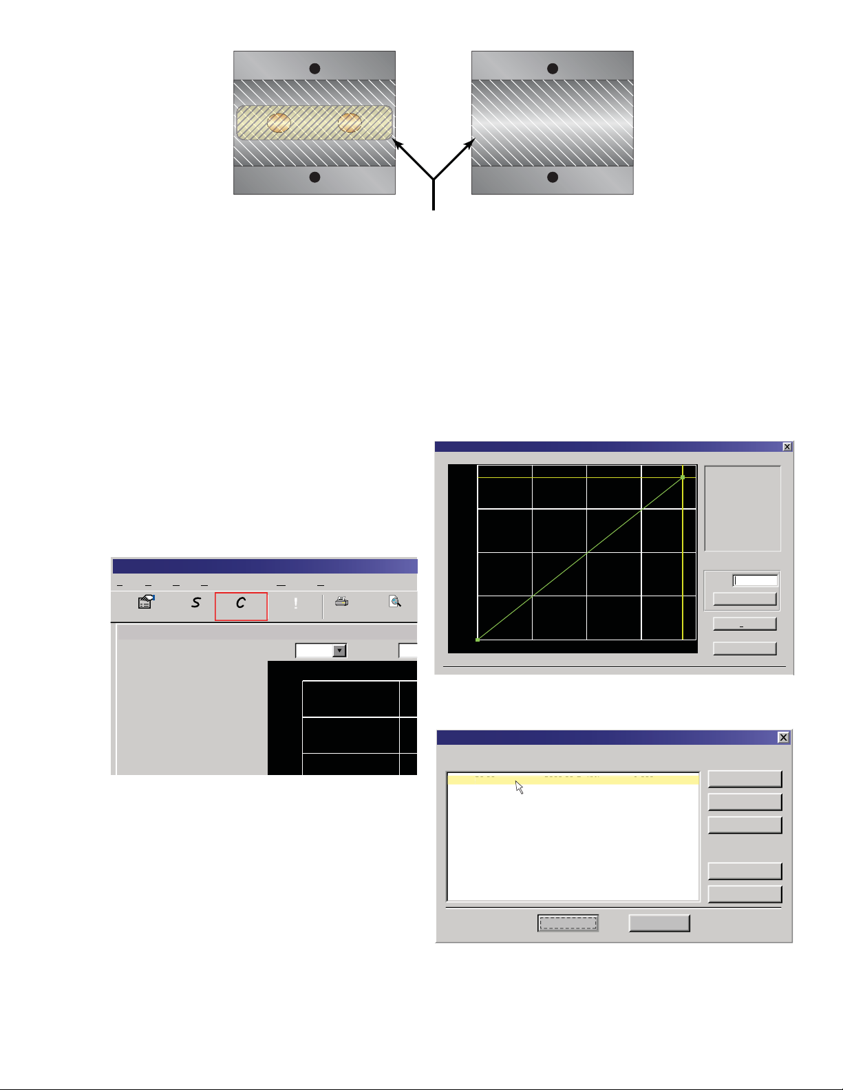
1) Establish communications with the transit
time meter. See Part 5 - Software Utility.

2) From the Tool Bar select Calibration. See
Figure 2.7.

3) On the pop-up screen, click Next button
twice to get to Page 3 of 3. See Figure 2.8.

Device Addr 127

HelpWindowCommunicationsViewEditFile

!

Configuration CalibrationStrategy

Device Addr 127

Errors

Print PreviePrint

Scale:60 MinTime:

Calibration (Page 3 of 3) - Linearization

28.2

Gal/M

200

Delta Time

1) Please establish a
reference flow rate.

1FPS / 0.3MPS Minimum.

2) Enter the reference flow
rate below. (Do not enter 0)

3) Wait for flow to stabilize.

4) Press the Set button.

Flow:

Set

Edit

Export...

Flow:

Totalizer Net:

Pos:

Neg:

Sig. Strength:

Margin:

Delta T:

Last Update:

1350 Gal/Min
0 OB
0 OB
0 OB

15.6%
100%

-2.50 ns
09:53:39

2000

1600

1200

FIGURE 2.7  DATA DISPLAY SCREEN

4) Click Edit.

5) If calibration point is displayed in Calibration
Points Editor screen, record the information,
highlight and click Remove. See Figure 2.9.

6) Click ADD...

7) Enter Delta T, Un-calibrated Flow, and Cali­brated Flow values from the FDT-41 through
FDT-46/FDT-41-HT through FDT-46-HT cali­bration label, the click OK. See Figure 2.10.

FIGURE 2.8  CALIBRATION PAGE 3 OF 3

Calibration Points Editor

Select point(s) to edit or remove:

30.00 ns 2000.00 Gal/Min 1.000

ns 2

OK

Min 1.

Cancel

FIGURE 2.9  CALIBRATION POINTS EDITOR

Add...

Edit...

Remove

Select All

Select All

Select None

Select None

25

8) Click OK in the Edit Calibration Points
screen.

9) Process will return to Page 3 of 3. Click
Finish. See Figure 2.8.

10) After “Writing Con guration File” is
complete, turn power o . Turn on again
to activate new settings.

Model: FDT-45-ANSI
S/N: 12345 Delta-T: 391.53nS

Uncal. Flow: 81.682 GPM

Cal. Flow: 80 GPM

Edit Calibration Points

Delta T:

Uncalibrated Flow:

Calibrated Flow:

OK

391.53

81.682

80.000

ns

Gal/Min.

Gal/Min.

Cancel

MOUNTING TRANSDUCERS IN

FIGURE 2.10  EDIT CALIBRATION POINTS

ZMOUNT CONFIGURATION

Installation on larger pipes requires careful measurements of the linear and radial placement of the
FDT-47, FDT-48, and FDT-47-HT transducers. Failure to properly orient and place the transducers on the
pipe may lead to weak signal strength and/or inaccurate readings. This section details a method for
properly locating the transducers on larger pipes. This method requires a roll of paper such as freezer
paper or wrapping paper, masking tape and a marking device.

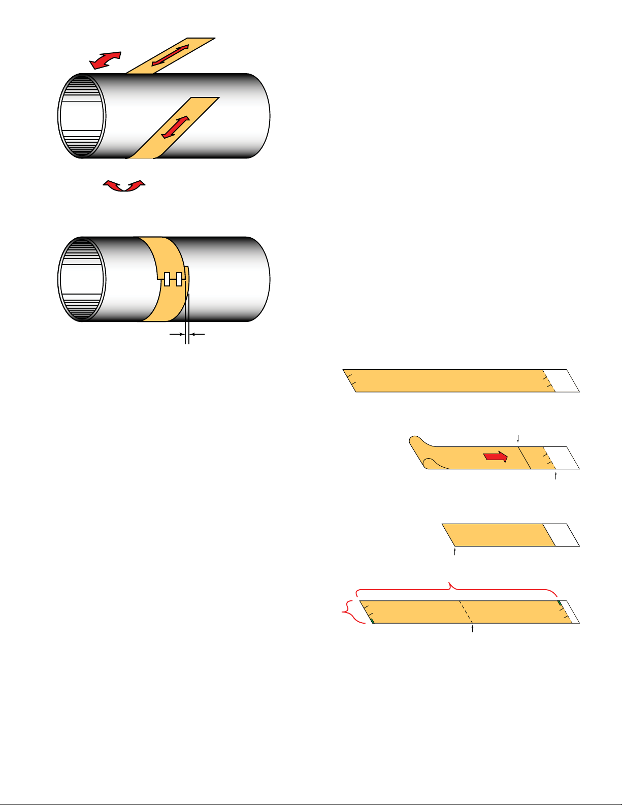
1) Wrap the paper around the pipe in the manner shown in Figure 2.11. Align the paper ends to
within ¼ inch (6 mm).

2) Mark the intersection of the two ends of the paper to indicate the circumference. Remove the
template and spread it out on a  at surface. Fold the template in half, bisecting the circumfer­ence. See Figure 2.12.

3) Crease the paper at the fold line. Mark the crease. Place a mark on the pipe where one of the
transducers will be located. See Figure 2.2 for acceptable radial orientations. Wrap the template
back around the pipe, placing the beginning of the paper and one corner in the location of the
mark. Move to the other side of the pipe and mark the pipe at the ends of the crease. Measure
from the end of the crease (directly across the pipe from the  rst transducer location) the dimen­sion derived in Step 2, Transducer Spacing. Mark this location on the pipe.

4) The two marks on the pipe are now properly aligned and measured.

If access to the bottom of the pipe prohibits the wrapping of the paper around the circumfer­ence, cut a piece of paper ½ the circumference of the pipe and lay it over the top of the pipe. The
length of ½ the circumference can be found by:

½ Circumference = Pipe O.D. × 1.57

The transducer spacing is the same as found in the Transducer Positioning section.

Mark opposite corners of the paper on the pipe. Apply transducers to these two marks.

26

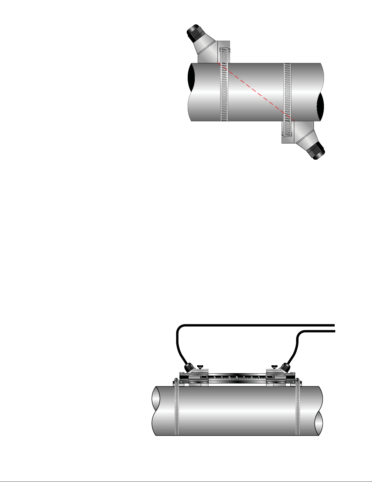
LESS THAN ¼” (6 mm)

7) Place the downstream transducer on the
pipe at the calculated transducer spacing.
See Figure 2.13. Using  rm hand pressure,
slowly move the transducer both towards
and away from the upstream transducer
while observing signal strength. Clamp
the transducer at the position where the
highest signal strength is observed. Signal
strength of between 5 and 98 is accept­able. The factory default signal strength
setting is 5, however there are many
application speci c conditions that may
prevent the signal strength from attaining
this level.

A minimum signal strength of 5 is accept­able as long as this signal level is main­tained under all  ow conditions.
On certain pipes, a slight twist to the
transducer may cause signal strength to
rise to acceptable levels.

FIGURE 2.11  PAPER TEMPLATE ALIGNMENT

5) For FDT-47, FDT-48, and FDT-47-HT
transducers, place a single bead of
couplent, approximately ½ inch (12
mm) thick, on the  at face of the
transducer. See Figure 2.4. Generally,
a silicone-based grease is used as an
acoustic couplent, but any good quality
grease-like substance that is rated to
not “ ow” at the temperature that the
pipe may operate at will be acceptable.

6) Place the upstream transducer in posi­tion and secure with a stainless steel
strap or other fastening device. Straps
should be placed in the arched groove
on the end of the transducer. A screw
is provided to help hold the trans­ducer onto the strap. Verify that the
transducer is true to the pipe, adjust
as necessary. Tighten transducer strap
securely. Larger pipes may require
more than one strap to reach the
circumference of the pipe.

Edge of

Paper

Line Marking

Circumference

Fold

Pipe Circumference

Transducer

Spacing

Crease

(Center of Pipe)

FIGURE 2.12  BISECTING THE PIPE CIRCUMFERENCE

27

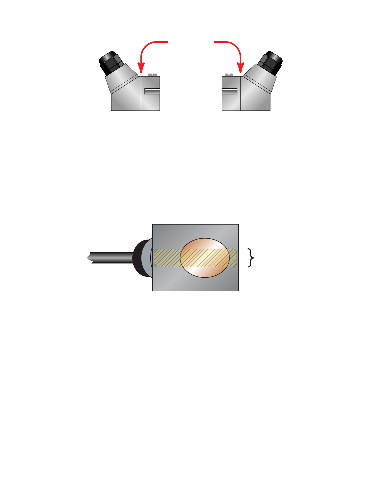
8) Certain pipe and liquid characteristics may
cause signal strength to rise to greater
than 98. The problem with operating this
meter with very high signal strength is that
the signals may saturate the input ampli­ ers and cause erratic readings. Strate­gies for lowering signal strength would
be changing the transducer mounting
method to the next longest transmis­sion path. For example, if there is exces­sive signal strength and the transducers
are mounted in a Z-Mount, try changing
to V-Mount or W-Mount. Finally you can
also move one transducer slightly o line
with the other transducer to lower signal
strength.

9) Secure the transducer with a stainless steel
strap or other fastener.

MOUNTING TRACK INSTALLATION

TOP VIEW

OF PIPE

FIGURE 2.13  ZMOUNT TRANSDUCER PLACEMENT

1) A convenient transducer mounting track can be used for pipes that have outside diameters
between 2 and 10 inches (50 and 250 mm). If the pipe is outside of that range, select a V-Mount
or Z-Mount mounting method.

2) Install the single mounting rail on the side of the pipe with the stainless steel bands provided. Do
not mount it on the top or bottom of the pipe. Orientation on vertical pipe is not critical. Ensure
that the track is parallel to the pipe and that all four mounting feet are touching the pipe.

3) Slide the two transducer clamp brackets towards the center mark on the mounting rail.

4) Place a single bead of couplent, approximately ½ inch (12 mm) thick, on the  at face of the trans­ducer. See Figure 2.4.

5) Place the  rst transducer in between the mounting rails near the zero point on the scale. Slide the
clamp over the transducer. Adjust the clamp/transducer such that the notch in the clamp aligns
with zero on the scale. See Figure 2.14.

6) Secure with the thumb screw. Ensure that the screw rests in the counter bore on the top of the
transducer. (Excessive pressure is
not required. Apply just enough
pressure so that the couplent  lls
the gap between the pipe and
transducer.)

7) Place the second transducer in
between the mounting rails near
the dimension derived in the
transducer spacing section. Read
the dimension on the mounting
rail scale. Slide the transducer
clamp over the transducer and
secure with the thumb screw.

Top View

of Pipe

28

FIGURE 2.14  MOUNTING TRACK INSTALLATION

PART 3  INPUTS/OUTPUTS

GENERAL

The  ow metering system is available in two general con gurations. There is the standard  ow meter
model that is equipped with a 4-20 mA output, two open collector outputs, a rate frequency output, and
RS485 communications using the

The energy version of the  ow metering family has inputs for two 1,000 Ohm RTD sensors in place of
the rate frequency and alarm outputs. This version allows the measurement of pipe input and output
temperatures so energy usage calculations can be performed.

420 mA OUTPUT

The 4-20 mA output interfaces with most recording and logging systems by transmitting an analog
current signal that is proportional to system  ow rate. The 4-20 mA output is internally powered (current
sourcing) and can span negative to positive  ow/energy rates.

For AC powered units, the 4-20 mA output is driven from a +15 VDC source located within the meter.
The source is isolated from earth ground connections within the  ow meter. The AC powered model
can accommodate loop loads up to 400 Ohms. DC powered meters utilize the DC power supply voltage
to drive the current loop. The current loop is not isolated from DC ground or power. Figure 3.1 shows
graphically the allowable loads for various input voltages. The combination of input voltage and loop
load must stay within the shaded area of Figure 3.1.

Modbus RTU command set.

Supply Voltage - 7 VDC

0.02

1100

1000

900
800
700
600
500
400

= Maximum Loop Resistance

Operate in the

Loop Load (Ohms)

300
200
100

10 12 14 16 18 20 22 24 26 28

Shaded Regions

Supply Voltage (VDC)

FIGURE 3.1  ALLOWABLE LOOP RESISTANCE DC POWERED UNITS

29

90-265 VAC
AC Neutral

Signal Ground

Signal Gnd.
Control 1

Loop

Resistance

Control 2
Frequency Out
4-20 mA Out
Reset Total

7 VDC

Drop

Meter Power

FIGURE 3.2  420 MA OUTPUT

The 4-20 mA output signal is available between the 4-20 mA Out and Signal Gnd terminals as shown in
Figure 3.2.

CONTROL OUTPUTS FLOW ONLY VERSION

Two independent open collector transistor outputs are included with the
 ow only model. Each output can be con gured for one of the following
four functions:

O

1234

N

Rate Alarm
Signal Strength Alarm
Totalizing/Totalizing Pulse
Errors
None

FIGURE 3.3  SWITCH SETTINGS

Both control outputs are rated for a maximum of 100 mA and 10 to 28 VDC. A pull-up resistor can be
added externally or an internal 10K Ohm pull-up resistor can be selected using DIP switches on the
power supply board.

Switch S1 S2 S3 S4

On

O

Control 1 Pull-Up
Resistor IN circuit

Control 1 Pull-Up

Resistor OUT of circuit

Control 2 Pull-Up
Resistor IN circuit

Control 2 Pull-Up

Resistor OUT of circuit

Frequency output Pull-Up

Resistor IN circuit

Frequency Output Pull-Up

Resistor OUT of circuit

Square Wave

Output

Simulated Turbine

Output

TABLE 3.1  DIP SWITCH FUNCTIONS

NOTE: All control outputs are disabled when USB cable is connected.

30

For the Rate Alarm and Signal Strength Alarm the on/o values are set using either the keypad or the
software utility.

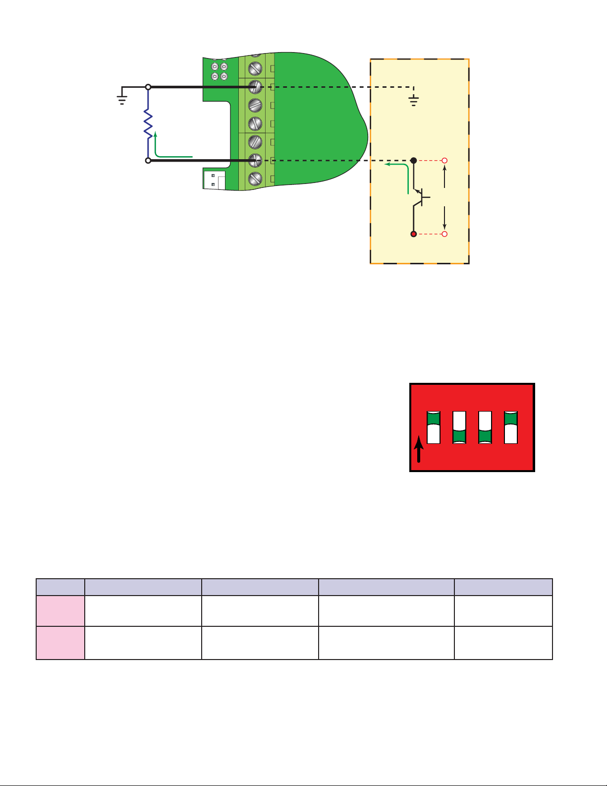
Typical control connections are illustrated in Figure 3.3. Please note that only the Control 1 output is
shown. Control 2 is identical except the pull-up resistor is governed by SW2.

VCC

O

1234

N

SW1/SW2

90-265 VAC
AC Neutral
Signal Gnd.
Control 1
Control 2
Frequency Out
4-20 mA Out
Reset Total

10K

O

1234

N

SW1/SW2

10 - 28

VDC

100 mA Maximum

90-265 VAC
AC Neutral
Signal Gnd.
Control 1
Control 2
Frequency Out
4-20 mA Out
Reset Total

FIGURE 3.4  TYPICAL CONTROL CONNECTIONS

Alarm Output

The  ow rate output permits output changeover at two separate  ow rates allowing operation with an
adjustable switch deadband. Figure 3.5 illustrates how the setting of the two set points in uences rate
alarm operation.

A single-point  ow rate alarm would place the ON setting slightly higher than the OFF setting allowing
a switch deadband to be established. If a deadband is not established, switch chatter (rapid switching)
may result if the  ow rate is very close to the switch point.

Minimum

Flow

Set OFF

Set ON

Output ON

Maximum

Flow

Output OFF

Deadband

FIGURE 3.5  SINGLE POINT ALARM OPERATION

NOTE: All control outputs are disabled when USB cable is connected.

31

Batch/Totalizer Output for Flow Only Version

Totalizer mode con gures the output to send a 33 mSec pulse each time the display totalizer increments
divided by the TOT MULT. The TOT MULT value must be a whole, positive, numerical value.

For example, if the totalizer exponent (TOTL E) is set to E0 (×1) and the totalizer multiplier (TOT MULT)
is set to 1, then the output will pulse each time the totalizer increments one count, or each single, whole
measurement unit totalized.

If the totalizer exponent (TOTL E) is set to E2 (×100) and the totalizer multiplier (TOT MULT) is set to 1,
then the control output will pulse each time the display totalizer increments or once per 100 measure­ment units totalized.

If the totalizer exponent (TOTL E) is set to E0 (×1) and the totalizer multiplier (TOT MULT) is set to 2, the
control output will pulse once for every two counts that the totalizer increments.

Totalizer Output Option for Energy Meter

Energy units can be ordered with a totalizer pulse output option. This option is installed in the position
where the Ethernet option would normally be installed.

OPTIONAL TOTALIZING PULSE SPECIFICATIONS

Optional FDT-40E Totalizing Pulse Output

Signal
Type
Pulse Width
Voltage

Current

Pull-up Resistor

NOTE: The totalizer pulse output option and the Ether­net communications output can not be installed in the
same energy unit at the same time.

Wiring and con guration of this option is
similar to the totalizing pulse output for the
 ow only variation. This option must use an
external current limiting resistor.

1 pulse for each increment of the totalizers least signi cant digit.
Opto-isolated, open collector transistor
30 mSec, maximum pulse rate 16 Hz.
28 VDC maximum.
100 mA maximum (current sink).

2.8 K Ohms to 10 K Ohms

Totalizing

Pulse Output

Option

Internal

V

CC

2.8K to 10K

100 mA

Maximum

RxD

TB1

Total Pulse

Pull-up

Resistor

Isolated Output

Total Pulse

32

FIGURE 3.6  ENERGY VERSION TOTALIZER OUTPUT OPTION

Signal Strength Alarm

The SIG STR alarm will provide an indication that the signal level reported by the transducers has fallen
to a point where  ow measurements may not be possible. It can also be used to indicate that the pipe
has emptied. Like the rate alarm described previously, the signal strength alarm requires that two points
be entered, establishing an alarm deadband. A valid switch point exists when the ON value is lower than
the OFF value. If a deadband is not established and the signal strength decreases to approximately the
value of the switch point, the output may “chatter”.

Error Alarm Outputs

When a control output is set to ERROR mode, the output will activate when any error occurs in the  ow
meter that has caused the meter to stop measuring reliably. See the Appendix of this manual for a list of
potential error codes.

+V

FREQUENCY OUTPUT FLOW ONLY UNITS

The frequency output is an open-collector
transistor circuit that outputs a pulse wave­form that varies proportionally with  ow rate.
This type of frequency output is also know as
a “Rate Pulse” output. The output spans from
0 Hz, normally at zero  ow rate to 1,000 Hz at

SW4 Closed
SW4 Open

90-265 VAC
AC Neutral
Signal Gnd.
Control 1
Control 2
Frequency Out
4-20 mA Out
Reset Total

O

1234

N

10K

full  ow rate (con guration of the MAX RATE
parameter is described in detail in the  ow

Frequency Output

meter con guration section of this manual).

FIGURE 3.7  FREQUENCY OUTPUT SWITCH SETTINGS

The frequency output is proportional to the maximum  ow rate entered into the meter. The maximum
output frequency is 1,000 Hz.

NOTE: When USB programming cable is connected, the RS485 and frequency outputs are disabled.

If, for example, the MAX RATE parameter was set to 400 GPM then an output frequency of 500 Hz (half of
the full scale frequency of 1,000 Hz) would represent 200 GPM.

In addition to the control outputs, the frequency output can be used to provide total information by use
of a “K-factor”. A K-factor simply relates the number of pulses from the frequency output to the number
of accumulated pulses that equates to a speci c volume.

For this meter the relationship is described by the following equation. The 60,000 relates to measure­ment units in volume/min. Measurement units in seconds, hours or days would require a di erent
numerator.

K factor



60,000

Full Scale Units



EQUATION 3.1  KFACTOR CALCULATION

33

A practical example would be if the MAX RATE for the application were 400 GPM, the K-factor (repre-
senting the number of pulses accumulated needed to equal 1 Gallon) would be:

K factor Pulses Per Gallon

 

60,000

400

GPM



150

If the frequency output is to be used as a totalizing output, the  ow meter and the receiving instrument
must have identical K-factor values programmed into them to ensure that accurate readings are being
recorded by the receiving instrument. Unlike standard mechanical  ow meters such as turbines, gear or
nutating disk meters, the K-factor can be changed by modifying the MAX RATE  ow rate value.

NOTE: For a full treatment of K-factors please see the Appendix of this manual.

There are two frequency output types available:

Turbine meter simulation - This option is utilized when a receiving instrument is capable of
interfacing directly with a turbine  ow meter’s magnetic pickup. The output is a relatively low
voltage AC signal whose amplitude swings above and below the signal ground reference. The
minimum AC amplitude is approximately 500 mV peak-to-peak. To activate the turbine output
circuit, turn SW4 OFF.

500 mV

p-p

0

FIGURE 3.8  FREQUENCY OUTPUT WAVEFORM SIMULATED TURBINE

Square-wave frequency - This option is utilized when a receiving instrument requires that the
pulse voltage level be either of a higher potential and/or referenced to DC ground. The output is
a square-wave with a peak voltage equaling the instrument supply voltage when the SW3 is ON.
If desired, an external pull-up resistor and power source can be utilized by leaving SW3 OFF. Set
SW4 to ON for a square-wave output.

+V

0

FIGURE 3.9  FREQUENCY OUTPUT WAVEFORM SQUARE WAVE

34

RS485

The RS485 feature allows up to 126  ow metering systems to be placed on a single three-wire cable bus.
All meters are assigned a unique numeric address that allows all of the meters on the cable network to
be independently accessed. A Modbus RTU command protocol is used to interrogate the meters. An
explanation of the command structure is detailed in the Appendix of this manual. Flow rate, total, signal
strength and temperature (if so equipped) can be monitored over the digital communications bus. Baud
rates up to 9600 and cable lengths to 5,000 feet (1,500 meters) are supported without repeaters or “end
of line” resistors.

To interconnect meters, utilize three-wire shielded cable such as Belden® 9939 or equal. In noisy envi­ronments the shield should be connected on one end to a good earth ground connection. A USB to
RS485 converter such as the B & B Electronics P/N 485USBTB-2W can be used to communicate with a
PC running Windows 98, Windows ME, Windows 2000, Windows NT, Windows XP, Windows Vista®, and
Windows® 7. For computers with RS232C serial ports, an RS232C to RS485 converter, such as B&B Elec­tronics P/N 485SD9TB (illustrated in Figure 3.10), is required to interconnect the RS485 network to a
communication port on a PC. If more than 126 meters must be monitored, an additional converter and
communication port are required.

NOTE: When USB programming cable is connected, the RS485 and frequency outputs are disabled.

TD(A)­TD(B)+

GND
GND

+12V

A (-)

B (+)

A (-)
B (+)
GND

4-20 mA Out
Reset Total
RS485 Gnd
RS485 A(-)
RS485 B(+)

USB to RS485

FIGURE 3.10  RS485 NETWORK CONNECTIONS

RS-232

RS-485

4-20 mA Out
Reset Total
RS485 Gnd
RS485 A(-)
RS485 B(+)

RS-485

To 12 VDC

Supply

Converte r

RS232 to RS485

35

HEAT FLOW FOR ENERGY UNITS ONLY

The energy version allows the integration of two 1000 Ohm, platinum
RTDs with the  ow meter, e ectively providing an instrument for
measuring energy consumed in liquid heating and cooling systems.
If RTDs were ordered with the energy version of the  ow meter, they
have been factory calibrated and are shipped with the meter.

The energy meter has multiple heat ranges to choose from. For best
resolution use the temperature range that encompasses the tempera­ture range of the application.

The three-wire surface mount RTDs are attached at the factory to a
simple plug-in connector eliminating the possibility of mis-wiring.
Simply install the RTDs on or in the pipe as recommended, and then
plug the RTDs into the RTD connector in the  ow meter.

Four ranges of surface mount RTDs and two lengths of wetted inser­tion probes are o ered. Other cable lengths for surface mount RTDs are
available. Contact the manufacturer for additional o erings.

All RTDs are 1,000 Ohm platinum, three-wire devices. The surface
mount versions are available in standard lengths of 20 feet (6 meters),
50 feet (15 meters) and 100 feet (30 meters) of attached shielded cable.

BACK OF

CONNECTOR



RETURN LINE

RTD #2



SUPPLY LINE

RTD #1

FIGURE 3.11  RTD SCHEMATIC

Installation of Surface Mount RTDs

Surface mount RTDs should only be utilized on well insulated pipe. If the area where the RTD is located
is not insulated, inconsistent temperature readings will result. Insertion (wetted) RTDs should be used on
pipes that are not insulated.

Select areas on the supply and return pipes where
the RTDs will be mounted. Remove or peel back
the insulation all the way around the pipe in the
installation area. Clean an area slightly larger than
the RTD down to bare metal on the pipe.

Place a small amount of heat sink compound
on the pipe in the RTD installation location.
See Figure 3.12. Press the RTD  rmly into the
compound. Fasten the RTD to the pipe with the
included stretch tape.

Clean RTD Mounting

Area to Bare Metal Surface

Heat Tape

MINCO

OT-201

Heat Sink

Compound

36

FIGURE 3.12  SURFACE MOUNT RTD INSTALLATION

Route the RTD cables back to the  ow meter and
secure the cable so that it will not be pulled on or
abraded inadvertently. Replace the insulation on
the pipe, ensuring that the RTDs are not exposed
to air currents.

Installation of Insertion RTDs

Insertion RTDs are typically installed through
¼ inch (6 mm) compression  ttings and isola­tion ball valves. Insert the RTD su ciently into
the  ow stream such that a minimum of ¼ inch
(6 mm) of the probe tip extends into the pipe
diameter.

RTDs should be mounted within ±45 degrees of
the side of a horizontal pipe. On vertical pipes
the orientation is not critical. Route the RTD
cables back to the  ow meter and secure the
cable so that it will not be pulled on or abraded
inadvertently.

If the cables are not long enough to reach the
 ow meter route the cables to an electrical

FIGURE 3.13  INSERTION STYLE RTD INSTALLATION

junction box and add additional cable from that
point. Use three-wire shielded cable, such as Belden® 9939 or equal, for this purpose.

NOTE: Adding cable adds to the resistance the meter reads and may have an
e ect on absolute accuracy. If cable is added, ensure that the same length is

Exc.
Sig.

Gnd.

Shield

+Vo

-Vo

RTD 1

RTD 2

TEMP. SET

Modbus

TFX Rx
TFX Tx

Exc.
Sig.
Gnd.
Shield

0 to 50°C

0 to 100°C

-40 to 200°C

added to both RTDs to minimize errors due to changes in cable resistance.

Wiring to Meter

After the RTDs have been mounted to

RTD #1

the pipe, route the cable back to the
 ow meter through the middle hole

RTD #2

in the enclosure. Connection to the

meter is accomplished by inserting
the RTD connector into the mating

connector on the circuit board. Be sure

RTD’s

SUPPLY LINE

MINCO

MINCO

RETURN LINE

372

VE

D

1500mA250V

C US

W

R

ACN

ACL

95 - 264 VAC

AC Neutral

Signal Gnd.
4-20 mA Out
Reset Total
RS485 Gnd
RS485 A(-)
RS485 B(+)

that the alignment tab on the RTD
cable is up.

Downstream

Upstream

-

-

+

+

FIGURE 3.14  CONNECTING RTDS

37

Replacement RTDs

If it is necessary to replace RTDs, complete RTD kits including the energy meter’s plug-in connector and
calibration values for the replacements are available.

It is also possible to use other RTDs. The RTDs must be 1,000 Ohm platinum RTDs suitable for a three­wire connection. A connection adapter, P.N. FDT-40-RTDCONN, is available to facilitate connection to the
energy version. See Figure 3.15.

WHITE

RTD2

RTD1

PIN#5
PIN#3
PIN#1

PIN#8
PIN#6

PIN#4
PIN#2

PIN #8
PIN #6

PIN #4
PIN #2

PIN #5

PIN #3
PIN #1

RED

BLACK

GREEN

BROWN

BLUE

DRAIN

WHITE
BLACK
RED

DRAIN
GREEN

BLUE
BROWN

FIGURE 3.15  ULTRASONIC ENERGY  RTD ADAPTER CONNECTIONS

NOTE: It will be necessary to calibrate third party RTDs to the  ow meter for proper operation. See the Appendix of this manual

for the calibration procedure.

38

PART 4  STARTUP AND CONFIGURATION

BEFORE STARTING THE INSTRUMENT

NOTE: This  ow metering system requires a full pipe of liquid before a successful start-up can be completed. Do not attempt to
make adjustments or change con gurations until a full pipe is veri ed.

NOTE: If Dow 732 RTV was utilized to couple the transducers to the pipe, the adhesive must be fully cured before readings are
attempted. Dow 732 requires 24 hours to cure satisfactorily. If Sonotemp® acoustic coupling grease was utilized as a couplent,
curing is not required.

INSTRUMENT STARTUP

Procedure:

1) Verify that all wiring is properly connected and routed, as described in Part 1 of this manual.

2) Verify that the transducers are properly mounted, as described in Part 2 of this manual.

3) Apply power. The display of the  ow meter will brie y show a software version number and then
all of the segments will illuminate in succession.

IMPORTANT!!: In order to complete the installation of the  ow meter, the pipe must be full of liquid.

To verify proper installation and  ow measurement operation:

1) Go to the SER MENU and con rm that signal strength (SIG STR) is between 5 and 98. If the signal
strength is lower than 5, verify that proper transducer mounting methods and liquid/pipe char­acteristics have been entered. To increase signal strength, if a W-Mount transducer installation
was selected, re-con gure for a V-Mount installation; if V-Mount was selected, re-con gure for
Z-Mount.

NOTE: Mounting con guration changes apply only to FDT-47, FDT-48 and FDT-47-HT transducer sets.

2) Verify that the actual measured liquid sound speed is very close to the expected value. The
measured liquid sound speed (SSPD FPS and SSPD MPS) is displayed in the SER MENU. Verify
that the measured sound speed is within 2% of the value entered as FLUID SS in the BSC MENU.
The pipe must be full of liquid in order to make this measurement.

Once the meter is operating properly, refer to the Keypad Programming section of this manual for addi­tional programming features.

39

KEYPAD PROGRAMMING

A meter ordered with a keypad can be con gured through the keypad interface or by using the
Windows® compatible software utility. Units without a keypad can only be con gured using the software
utility. See Part 5 of this manual for software details. Of the two methods of con guration, the software
utility provides more advanced features and o ers the ability to store and transfer meter con gurations
between like  ow meters. All entries are saved in non-volatile FLASH memory and will be retained inde ­nitely in the event of power loss.

NOTE: When USB programming cable is connected, the RS485 and frequency outputs are disabled.

The  ow meter versions with a keypad contain a four-key tactile feedback keypad interface that allows
the user to view and change con guration parameters used by the operating system.

Mode

Keypad

Indicators

FIGURE 4.1  KEYPAD INTERFACE

1) The MENU key is pressed from RUN mode to enter PROGRAM mode. The MENU key is pressed
in PROGRAM mode to exit from con guration parameter selection and menus. If changes to any
con guration parameters are made, the user will be prompted with a SAVE? when returning to
RUN mode. If YES is chosen the new parameters will be saved in program memory.

2) The arrow keys are used to scroll through menus and con guration parameters. The arrow
keys are also used to adjust parameter numerical values.

3) The ENTER key functions are:

~ Pressed from the RUN mode to view the current software version operating in the instrument.
~

Used to access the con guration parameters in the various menus.

~ Used to initiate changes in con guration parameters.
~

Used to accept con guration parameter changes.

40

MENU STRUCTURE

The  ow meters  rmware uses a hierarchical menu structure. A map of the user interface is included in
the Appendix of this manual. The map provides a visual path to the con guration parameters that users
can access. This tool should be employed each time con guration parameters are accessed or revised.

The seven menus used in the  ow meter  rmware are as follows:

BSC MENU

CH1 MENU

CH2 MENU

SEN MENU

SEC MENU

SER MENU

DSP MENU DISPLAY -- The display menu is used to con gure meter display functions.

The following sections de ne the con guration parameters located in each of the menus.

BASIC -- This menu contains all of the con guration parameters necessary to
initially program the meter to measure  ow.

CHANNEL 1 -- Con gures the 4-20 mA output. Applies to both the  ow only
and energy models.

CHANNEL 2 -- Con gures the type and operating parameters for channel 2 out­put options. Channel 2 parameters are speci c to the model of transmitter used.

SENSOR -- This menu is used to select the sensor type (i.e. FDT-47, FDT-41
through FDT-46, etc.)

SECURITY -- This menu is utilized for resetting totalizers, returning  ltering to
factory settings, and revising security the password.

SERVICE -- The service menu contains system settings that are used for
advanced con guration and zeroing the meter on the pipe.

BSC MENU  BASIC MENU

The BASIC menu contains all of the con guration parameters necessary to make the  ow meter
operational.

Units Selection

UNITS -- Programming Unit Selection (Choice)
ENGLSH (Inches)
METRIC (Millimeters)

Installs a global measurement standard into the memory of the instrument. The choices are either
English or Metric units.

Select ENGLSH if all con gurations (pipe sizes, etc.) are to be made in inches. Select METRIC if the
meter is to be con gured in millimeters.

The ENGLSH/METRIC selection will also con gure the  ow meter to display sound speeds in pipe
materials and liquids as either feet per second (FPS) or meters per second (MPS), respectively.

41

IMPORTANT!: If the UNITS entry has been changed from ENGLSH to METRIC or from METRIC to ENGLSH, the entry must be
saved and the instrument reset (power cycled or System Reset SYS RSET entered) in order for the  ow meter to initiate the change
in operating units. Failure to save and reset the instrument will lead to improper transducer spacing calculations and an instru­ment that may not measure properly.

Address

ADDRESS -- Modbus Address (Value)
1-126

NOTE: This is for the RS485 connection only. The Modbus TCP/IP address is set via the integrated HTML application in the Ethernet
port.

Each meter connected on the communications bus must have an unique address number assigned.

Transducer Mount

XDCR MNT -- Transducer Mounting Method (Choice)
V
W
Z

Selects the mounting orientation for the transducers. The selection of an appropriate mounting orienta­tion is based on pipe and liquid characteristics. See Part 2 - Transducer Installation in this manual.

Flow Direction

FLOW DIR -- Transducer Flow Direction Control (Choice)
FORWARD
REVERSE

Allows the change of the direction the meter assumes is forward. When mounting meters with integral
transducers this feature allows upstream and downstream transducers to be “electronically” reversed
making upside down mounting of the display unnecessary.

Transducer Frequency

XDCR HZ -- Transducer Transmission Frequency (Choice)
500 KHZ (500 Kilohertz)
1 MHZ (1 Megahertz)
2 MHZ (2 Megahertz)

Transducer transmission frequencies are speci c to the type of transducer and the size of pipe. In general
the FDT-48 500 KHz transducers are used for pipes greater than 24 inches (600 mm). FDT-47 and FDT­47-HT, 1 MHz transducers, are for intermediate sized pipes between 2 inches (50 mm) and 24 inches (600
mm). The FDT-41 through FDT-46 and FDT-41-HT through FDT-46-HT, 2 MHz transducers, are for pipe
sizes between ½ inch (13 mm) and 2 inches (50 mm)

42

Pipe Outside Diameter

PIPE OD -- Pipe Outside Diameter Entry (Value)
ENGLSH (Inches)
METRIC (Millimeters)

Enter the pipe outside diameter in inches if ENGLSH was selected as UNITS; in millimeters if METRIC was
selected.

NOTE: Charts listing popular pipe sizes have been included in the Appendix of this manual. Correct entries for pipe O.D. and pipe
wall thickness are critical to obtaining accurate  ow measurement readings.

Pipe Wall Thickness

PIPE WT -- Pipe Wall Thickness Entry (Value)
ENGLSH (Inches)
METRIC (Millimeters)

Enter the pipe wall thickness in inches if ENGLSH was selected as UNITS; in millimeters if METRIC was
selected.

NOTE: Charts listing popular pipe sizes have been included in the Appendix of this manual. Correct entries for pipe O.D. and pipe
wall thickness are critical to obtaining accurate  ow measurement readings.

Pipe Material

PIPE MAT -- Pipe Material Selection (Choice)

Acrylic (ACRYLIC) Glass Pyrex (PYREX) St Steel 304/316 (SS 316)
Aluminum (ALUMINUM) Nylon (NYLON) St Steel 410 (SS 410)
Brass (Naval) (BRASS) HD Polyethylene (HDPE) St Steel 430 (SS 430)
Carbon Steel (CARB ST) LD Polyethylene (LDPE) PFA (PFA)
Cast Iron (CAST IRN) Polypropylene (POLYPRO) Titanium (TITANIUM)
Copper (COPPER) PVC CPVC (PVC/CPVC) Asbestos ASBESTOS
Ductile Iron (DCTL IRN) PVDF (PVDF) Other (OTHER)
Fiberglass-Epoxy (FBRGLASS) St Steel 302/303 (SS 303)

This list is provided as an example. Additional pipe materials are added periodically. Select the appro­priate pipe material from the list or select OTHER if the material is not listed.

43

Pipe Sound Speed

PIPE SS -- Speed of Sound in the Pipe Material (Value)
ENGLSH (Feet per Second)
METRIC (Meters per Second)

Allows adjustments to be made to the speed of sound value, shear or transverse wave, for the pipe wall.
If the UNITS value was set to ENGLSH, the entry is in FPS (feet per second). METRIC entries are made in
MPS (meters per second).

If a pipe material was chosen from the PIPE MAT list, a nominal value for speed of sound in that material
will be automatically loaded. If the actual sound speed is known for the application piping system and
that value varies from the automatically loaded value, the value can be revised.

If OTHER was chosen as PIPE MAT, then a PIPE SS must also be entered.

Pipe Roughness

PIPE R -- Pipe Material Relative Roughness (Value)
Unitless Value

The  ow meter provides  ow pro le compensation in its  ow measurement calculation. The ratio of
average surface imperfection as it relates to the pipe internal diameter is used in this compensation algo­rithm and is found by using the following formula:

    

Linear RMS Measurement of the Pipes Internal Wall Surface

Pipe



   



Inside Diamet



er of the PipRe

If a pipe material was chosen from the PIPE MAT list, a nominal value for relative roughness in that mate-
rial will be automatically loaded. If the actual roughness is known for the application piping system and
that value varies from the automatically loaded value, the value can be revised.

Liner Thickness

LINER T -- Pipe Liner Thickness (Value)
ENGLSH (Inches)
METRIC (Millimeters)

If the pipe has a liner, enter the pipe liner thickness. Enter this value in inches if ENGLSH was selected as
UNITS; in millimeters if METRIC was selected.

44

Liner Material

LINER MA - Pipe Liner Material (Choice)
Liner Type - (If a LINER Thickness was selected)

Tar Epoxy (TAR EPXY) HD Polyethylene (HDPE)
Rubber (RUBBER) LD Polyethylene (LDPE)
Mortar (MORTAR) Te on (PFA) (TEFLON)
Polypropylene (POLYPRO) Ebonite (EBONITE)
Polystyrene (POLYSTY) Other (OTHER)

This list is provided as an example. Additional materials are added periodically. Select the appropriate
material from the list or select OTHER if the liner material is not listed.

Liner Sound Speed

LINER SS -- Speed of Sound in the Liner (Value)
ENGLSH (Feet per Second)
METRIC (Meters per Second)

Allows adjustments to be made to the speed of sound value, shear or transverse wave, for the pipe wall.
If the UNITS value was set to ENGLSH, the entry is in FPS (feet per second). METRIC entries are made in
MPS (meters per second).

If a liner was chosen from the LINER MA list, a nominal value for speed of sound in that media will be
automatically loaded. If the actual sound speed rate is known for the pipe liner and that value varies
from the automatically loaded value, the value can be revised.

Liner Roughness

LINER R -- Liner Material Relative Roughness (Value)
Unitless Value

The  ow meter provides  ow pro le compensation in its  ow measurement calculation. The ratio of
average surface imperfection as it relates to the pipe internal diameter is used in this compensation and
is found by using the following formula:

Liner R



Linear RMS Measurement of the Liners Internal Wall Surface

   

   



Inside Diameter of the Liner



If a liner material was chosen from the LINER MA list, a nominal value for relative roughness in that
material will be automatically loaded. If the actual roughness is known for the application liner and that
value varies from the automatically loaded value, the value can be revised.

45

Fluid Type

FL TYPE -- Fluid/Media Type (Choice)

Water Tap (WATER) Ethanol (ETHANOL) Oil Diesel (DIESEL)
Sewage-Raw (SEWAGE) Ethylene Glycol (ETH-GLYC) Oil Hydraulic [Petro-based] (HYD OIL)
Acetone (ACETONE) Gasoline (GASOLINE) Oil Lubricating (LUBE OIL)
Alcohol (ALCOHOL) Glycerin (GLYCERIN) Oil Motor [SAE 20/30] (MTR OIL)
Ammonia (AMMONIA) Isopropyl Alcohol (ISO-ALC) Water Distilled (WATR-DST)
Benzene (BENZENE) Kerosene (KEROSENE) Water Sea (WATR-SEA)
Brine (BRINE) Methanol (METHANOL) Other (OTHER)

This list is provided as an example. Additional liquids are added periodically. Select the appropriate liquid
from the list or select OTHER if the liquid is not listed.

Fluid Sound Speed

FLUID SS -- Speed of Sound in the Fluid (Value)
ENGLSH (Feet per Second)
METRIC (Meters per Second)

Allows adjustments to be made to the speed of sound entry for the liquid. If the UNITS value was set to
ENGLSH, the entry is in FPS (feet per second). METRIC entries are made in MPS (meters per second).

If a  uid was chosen from the FL TYPE list, a nominal value for speed of sound in that media will be auto­matically loaded. If the actual sound speed is known for the application  uid and that value varies from
the automatically loaded value, the value can be revised.

If OTHER was chosen as FL TYPE, a FLUID SS will need to be entered. A list of alternate  uids and their
associated sound speeds is located in the

Fluid sound speed may also be found using the Target DBg Data screen available in the software utility.

See Part 5.

Appendix located at the back of this manual.

Fluid Viscosity

FLUID VI -- Absolute Viscosity of the Fluid (Value - cP)

Allows adjustments to be made to the absolute viscosity of the liquid in centipoise.

Ultrasonic  ow meters utilize pipe size, viscosity and speci c gravity to calculate Reynolds numbers.
Since the Reynolds number in uences  ow pro le, the  ow meter has to compensate for the relatively
high velocities at the pipe center during transitional or laminar  ow conditions. The entry of FLUID VI is
utilized in the calculation of Reynolds and the resultant compensation values.

46

If a  uid was chosen from the FL TYPE list, a nominal value for viscosity in that media will be automati­cally loaded. If the actual viscosity is known for the application  uid and that value varies from the auto­matically loaded value, the value can be revised.

If OTHER was chosen as FL TYPE, then a FLUID VI must also be entered. A list of alternate  uids and their
associated viscosities is located in the

Appendix of this manual.

Fluid Speci c Gravity

SP GRAVTY -- Fluid Speci c Gravity Entry (Value)
Unitless Value

Allows adjustments to be made to the speci c gravity (density relative to water) of the liquid.

As stated previously in the FLUID VI section, speci c gravity is utilized in the Reynolds correction algo-
rithm. It is also utilized if mass  ow measurement units are selected for rate or total.

If a  uid was chosen from the FL TYPE list, a nominal value for speci c gravity in that media will be auto­matically loaded. If the actual speci c gravity is known for the application  uid and that value varies from
the automatically loaded value, the value can be revised.

If OTHER was chosen as FL TYPE, a SP GRVTY may need to be entered if mass  ows are to be calculated.
A list of alternate  uids and their associated speci c gravities is located in the

Appendix of this manual.

Fluid Speci c Heat Capacity

SP HEAT -- Fluid Speci c Heat Capacity (Value)
BTU/lb

Allows adjustments to be made to the speci c heat capacity of the liquid.

If a  uid was chosen from the FL TYPE list, a default speci c heat will be automatically loaded. This
default value is displayed as SP HEAT in the BSC MENU. If the actual speci c heat of the liquid is known
or it di ers from the default value, the value can be revised. See Tables 4.1, 4.2, and 4.3 for speci c
values. Enter a value that is the mean of both pipes.

Speci c Heat Capacity for Water

Temperature

°F °C

32-212 0-100 1.00
250 121 1.02

Speci c Heat

BTU/lb °F

300 149 1.03
350 177 1.05

TABLE 4.1  SPECIFIC HEAT CAPACITY VALUES FOR WATER

47

Speci c Heat Capacity Values for Common Fluids

Fluid

Speci c Heat BTU/lb °F

°F °C

Ethanol 32 0 0.65
Methanol 54 12 0.60
Brine 32 0 0.71
Brine 60 15 0.72
Sea Water 63 17 0.94

TABLE 4.2  SPECIFIC HEAT CAPACITY VALUES FOR OTHER COMMON FLUIDS

Speci c Heat Capacity BTU/lb °F
Temperature Ethylene Glycol Solution (% by Volume)
°F °C 25 30 40 50 60 65 100

-40 -40 n/a n/a n/a n/a 0.68 0.70 n/a
0 -17.8 n/a n/a 0.83 0.78 0.72 0.70 0.54
40 4.4 0.91 0.89 0.845 0.80 0.75 0.72 0.56
80 26.7 0.92 0.90 0.86 0.82 0.77 0.74 0.59
120 84.9 0.93 0.92 0.88 0.83 0.79 0.77 0.61
160 71.1 0.94 0.93 0.89 0.85 0.81 0.79 0.64

Temperature

200 93.3 0.95 0.94 0.91 0.87 0.83 0.81 0.66
240 115.6 n/a n/a n/a n/a n/a 0.83 0.69

TABLE 4.3  SPECIFIC HEAT CAPACITY VALUES FOR ETHYLENE GLYCOL/WATER

Transducer Spacing

XDC SPAC -- Transducer Spacing Calculation (Value)
ENGLSH (Inches)
METRIC (Millimeters)

NOTE: This value is calculated by the  rmware after all pipe parameters have been entered. The spacing value only pertains to
FDT-47, FDT-48, and FDT-47-HT transducer sets.

This value represents the one-dimensional linear measurement between the transducers (the upstream/
downstream measurement that runs parallel to the pipe). This value is in inches if ENGLSH was selected
as UNITS; in millimeters if METRIC was selected. This measurement is taken between the lines which are
scribed into the side of the transducer blocks.

If the transducers are being mounted using the transducer track assembly, a measuring scale is etched
into the track. Place one transducer at 0 and the other at the appropriate measurement.

48

Rate Units

RATE UNT -- Engineering Units for Flow Rate (Choice)

Gallons (Gallons) Pounds (LB)
Liters (Liters) Kilograms (KG)
Millions of Gallons (MGal) British Thermal Units (BTU)
Cubic Feet (Cubic Ft) Thousands of BTUs (MBTU)
Cubic Meters (Cubic Me) Millions of BTUs (MMBTU)
Acre Feet (Acre Ft) Tons (TON)
Oil Barrels (Oil Barr) [42 Gallons] Kilojoule (kJ)
Liquid Barrels (Liq Barr) [31.5 Gallons] Kilowatt (kW)
Feet (Feet) Megawatt (MW)
Meters (Meters)

Select a desired engineering unit for  ow rate measurements.

Rate Interval

RATE INT -- Time Interval for Flow Rate (Choice)
SEC Seconds
MIN Minutes
HOUR Hours
DAY Days

Select a desired engineering unit for  ow rate measurements.

Totalizer Units

TOTL UNT -- Totalizer Units

Gallons (Gallons) Pounds (LB)
Liters (Liters) Kilograms (KG)
Millions of Gallons (MGal) British Thermal Units (BTU)
Cubic Feet (Cubic Ft) Thousands of BTUs (MBTU)
Cubic Meters (Cubic Me) Millions of BTUs (MMBTU)
Acre Feet (Acre Ft) Tons (TON)
Oil Barrels (Oil Barr) [42 Gallons] Kilojoule (kJ)
Liquid Barrels (Liq Barr) [31.5 Gallons] Kilowatt (kW)
Feet (Feet) Megawatt (MW)
Meters (Meters)

Select a desired engineering unit for  ow accumulator (totalizer) measurements.

49

Totalizer Exponent

Exponent Display Multiplier

TOTL E -- Flow Totalizer Exponent Value (Choice)

E-1 × 0.1 (÷10)

E(-1) to E6

E0 × 1 (no multiplier)
E1 × 10

Utilized for setting the  ow totalizer exponent. This feature is useful
for accommodating a very large accumulated  ow or to increase
totalizer resolution when  ows are small (displaying fractions of
whole barrels, gallons, etc.) The exponent is a × 10

n

multiplier, where
“n” can be from –1 (× 0.1) to +6 (× 1,000,000). Table 4.4 should be
referenced for valid entries and their in uence on the display. Selec­tion of E-1 and E0 adjusts the decimal point on the display. Selection

E2 × 100
E3 × 1,000
E4 × 10,000
E5 × 100,000
E6 × 1,000,000

TABLE 4.4  EXPONENT VALUES

of E1, E2 and E3 causes an icon of × 10, × 100 or × 1000 respectively
to appear to the right of the total  ow display value.

Minimum Flow Rate

MIN RATE -- Minimum Flow Rate Settings (Value)

A minimum rate setting is entered to establish  lter software settings and the lowest rate value that will
be displayed. Volumetric entries will be in the Rate Units and Interval selected on Page 49 of this manual.
For unidirectional measurements, set MIN RATE to zero. For bidirectional measurements, set MIN RATE
to the highest negative (reverse)  ow rate expected in the piping system.

NOTE: The  ow meter will not display a  ow rate at  ows less than the MIN RATE value. As a result, if the MIN RATE is set to a
value greater than zero, the  ow meter will display the MIN RATE value, even if the actual  ow/energy rate is less than the MIN
RATE.

For example, if the MIN RATE is set to 25 and actual rate is 0, the meter display will indicate 25. Another example, if the MIN RATE
is set to -100 and the actual  ow is -200, the meter will indicate -100. This can be a problem if the meter MIN RATE is set to a value
greater than zero because at  ows below the MIN RATE the rate display will show zero  ow, but the totalizer which is not

a ected by the MIN RATE setting will keep totalizing.

Maximum Flow Rate

MAX RATE -- Maximum Flow Rate Settings (Value)

A maximum volumetric  ow rate setting is entered to establish  lter software settings. Volumetric entries
will be in the Rate Units and Interval selected on Page 49 of this manual. For unidirectional measure­ments, set MAX RATE to the highest (positive)  ow rate expected in the piping system. For bidirectional
measurements, set MAX RATE to the highest (positive)  ow rate expected in the piping system.

50

Low Flow Cut-o

FL C-OFF -- Low Flow Cut-o (Value)
0-100%

A low  ow cut-o entry is provided to allow very low  ow rates (that can be present when pumps are o
and valves are closed) to be displayed as zero  ow. Typical values that should be entered are between

1.0% and 5.0% of the  ow range between MIN RATE and MAX RATE.

Damping Percentage

DAMP PER -- System Damping (Value)
0-100%

Flow  lter damping establishes a maximum adaptive  lter value. Under stable  ow conditions ( ow
varies less than 10% of reading), this adaptive  lter will increase the number of successive  ow readings
that are averaged together up to this maximum value. If  ow changes outside of the 10% window, the
 ow  lter adapts by decreasing the number of averaged readings which allows the meter to react faster.
Increasing this value tends to provide smoother steady-state  ow readings and outputs. If very erratic
 ow conditions are present or expected, other  lters are available for use in the software utility. See Part 5
of this manual for further information.

51

CH1 MENU  CHANNEL 1 MENU

CH1 MENU -- 4-20 mA Output Menu

4-20 MA -- 4-20 mA Setup Options (Values)
FL 4MA Flow at 4 mA
FL 20MA Flow at 20 mA
CAL 4MA 4 mA Calibration
CAL 20MA 20 mA Calibration
4-20 TST 4-20 mA Test

The CH1 menu controls how the 4-20 mA output is spanned for all  ow meter models and how the
frequency output is spanned for the  ow only model.

The FL 4MA and FL 20MA settings are used to set the span for both the 4-20 mA output and the 0-1,000
Hz frequency output on the  ow only meter versions.

The 4-20 mA output is internally powered (current sourcing) and can span negative to positive  ow/
energy rates. This output interfaces with virtually all recording and logging systems by transmitting an
analog current that is proportional to system  ow rate. Independent 4 mA and 20 mA span settings are
established in  rmware using the  ow measuring range entries. These entries can be set anywhere in
the - 40 to + 40 FPS (-12 to +12 MPS) range of the instrument. Resolution of the output is 12-bits (4096
discrete points) and the can drive up to a 400 Ohm load when the meter is AC powered. When powered
by a DC supply, the load is limited by the input voltage supplied to the instrument. See Figure 3.1 for
allowable loop loads.

FL 4MA -- Flow at 4 mA
FL 20MA -- Flow at 20 mA

The FL 4MA and FL 20MA entries are used to set the span of the 4-20 mA analog output and the
frequency output on  ow only versions. These entries are volumetric rate units that are equal to the volu­metric units con gured as RATE UNT and RATE INT discussed on Page 49.

For example, to span the 4-20 mA output from -100 GPM to +100 GPM, with 12 mA being 0 GPM, set the
FL 4MA and FL 20MA inputs as follows:

FL 4MA = -100.0
FL 20MA = 100.0

If the meter were a  ow only model, this setting would also set the span for the frequency output. At

-100 GPM, the output frequency would be 0 Hz. At the maximum  ow of 100 GPM, the output frequency
would be 1,000 Hz, and in this instance a  ow of zero would be represented by an output frequency of
500 Hz.

52

Example 2 - To span the 4-20 mA output from 0 GPM to +100 GPM, with 12 mA being 50 GPM, set the FL
4MA and FL 20MA inputs as follows:

FL 4MA = 0.0
FL 20MA = 100.0

For the  ow only unit, in this instance zero  ow would be represented by 0 Hz and 4 mA. The full scale
 ow or 100 GPM would be 1,000 Hz and 20 mA, and a midrange  ow of 50 GPM would be expressed as
500 Hz and 12 mA.

The 4-20 mA output is factory calibrated and should not require adjustment. If small adjustments to the
DAC (Digital to Analog Converter) are needed, for instance if adjustment due to the accumulation of line
losses from long output cable lengths are required, the CAL 4mA and CAL 20 MA can be used.

CAL 4 MA -- 4 mA DAC Calibration Entry (Value)
CAL 20 MA-- 20 mA DAC Calibration Entry (Value)

The CAL 4MA and CAL 20 MA entries allow  ne adjustments to be made to the “zero” and full scale of
the 4-20 mA output. To adjust the outputs, an ammeter or reliable reference connection to the 4-20 mA
output must be present.

NOTE: Calibration of the 20 mA setting is conducted much the same way as the 4 mA adjustments.

NOTE: The CAL 4MA and CAL 20MA entries should not be used in an attempt to set the 4-20 mA range. Utilize FL 4MA and FL
20MA, detailed above, for this purpose.

4 mA Calibration Procedure:

1) Disconnect one side of the current loop and connect the ammeter in series (disconnect either
wire at the terminals labeled 4-20 mA Out or Signal Gnd).

2) Using the arrow keys, increase the numerical value to increase the current in the loop to 4 mA.
Decrease the value to decrease the current in the loop to 4 mA. Typical values range between
40-80 counts.

3) Reconnect the 4-20 mA output circuitry as required.

20 mA Calibration Procedure:

1) Disconnect one side of the current loop and connect the ammeter in series (disconnect either
wire at the terminals labeled 4-20 mA Out or Signal Gnd).

2) Using the arrow keys, increase the numerical value to increase the current in the loop to 20 mA.
Decrease the value to decrease the current in the loop to 20 mA. Typical values range between
3700-3900 counts.

3) Reconnect the 4-20 mA output circuitry as required.

4-20 TST -- 4-20 mA Output Test (Value)

Allows a simulated  ow value to be sent from the 4-20 mA output. By incrementing this value, the 4-20
mA output will transmit the indicated current value.

53

CH2 MENU  CHANNEL 2 MENU

The CH2 menu is used to con gure model speci c I/O options. The  ow only unit presents a di erent set
of parameters than the energy meter.

CAUTION

Caution: It is possible to choose options pertaining only to the  ow only meter when an energy meter
is present. The opposite is also true. The proper menu type must be chosen for the actual meter. If this
caution isn’t followed, the outputs or meter readings will be unpredictable.

Channel 2 Options

CH2 Menu -- Channel 2 I/O Options (Choice)
RTD -- Input Values for Energy Meters (Values)
CONTROL/HZ -- Output Options for Flow Only Meters

Energy Meter Options

RTD -- Calibration Values (Value)
RTD1 A Calibration Value for RTD1 A
RTD1 B Calibration Value for RTD1 B
RTD2 A Calibration Value for RTD2 A
RTD2 B Calibration Value for RTD2 B

Inputs from two 1,000 Ohm platinum RTD temperature sensors allow measurements of heating or
cooling usage.

The values used to calibrate the RTD temperature sensors are derived in the laboratory and are speci c
to the RTD and to the electronic circuit it is connected to. The RTDs on new units come with the calibra­tion values already entered into the energy meter and should not need to be changed.

Field replacement of RTDs is possible thru the use of the keypad or the software utility. If the RTDs were
ordered from the manufacturer, they will come with calibration values that need to be loaded into the
energy meter.

New, non-calibrated RTDs will need to be  eld calibrated using an ice bath and boiling water to derive
calibration values. This procedure is outlined in the

SURFACE MOUNT RTDS

FDT-40-RTD1 set of two, 200 °C Maximum Temperature (20 feet of cable)

INSERTION RTD

FDT-40-RTD2 single, 3 inch (75 mm), 0.25 inch OD
FDT-40-RTD3 single, 6 inch (150 mm), 0.25 inch OD

Appendix of this manual.

S

54

TABLE 4.5  RTDs

Flow Only Meter Options

Two independent open collector transistor outputs are included with the  ow only model. Each output
can be con gured independently for one of the following:

CONTROL/HZ -- Control Options (Choice)

Select either Control 1 or Control 2 to program.

TOTALIZE -- Totalizer Output Options

TOT MULT --Totalizer Multiplier (Value)

Sets the multiplier value applied to the totalizing pulse output.

FLOW -- Flow Alarm Output Options
FLOW -- Flow Alarm Values
ON (Value)

Sets value at which the alarm output will turn ON.

OFF (Value)

Sets value at which the alarm output will turn OFF.

SIG STR -- Signal Strength Alarm Options
SIG STR -- Signal Strength Alarm Values
ON (Value)

Sets value at which the alarm output will turn ON.

OFF (Value)

Sets value at which the alarm output will turn OFF.

ERRORS

Alarm outputs on any error condition. See Error Table in the

Appendix of this manual.

NONE

Alarm outputs disabled.

NOTE: The setup options for both CONTROL 1 and CONTROL 2 follow the same menu path. For a complete view of the menu
options, see the Menu Map in the

Appendix of this manual.

55

SEN MENU  SENSOR MENU

The SEN MENU allows access to the various types of transducers the meter can work with. Selecting the
proper transducers in conjunction with the transducer mount (XDCR MNT) and transducer frequency
(XDCR HZ) is critical to accurate operation of the meter.

SEN MENU -- Transducer Selection Menu (Choice)

FDT-47
Used on pipes 2 inches (51 mm) and larger.

(250 °F/121 °C maximum)

FDT-47-HT
High temperature version of FDT-47.

(350 °F/177 °C maximum)

FDT-48
Used on pipes 24 inches (600 mm) and larger.

(250 °F/121 °C maximum)

For pipes 24” (600 mm) and larger the FDT-48 transducers using a transmission frequency of
500 KHz are recommended.

FDT-48 transducers may also be advantageous on pipes between 4” and 24” if there are less
quanti able complicating aspects such as, sludge, tuberculation, scale, rubber liners, plastic
liners, thick mortar, gas bubbles, suspended solids, emulsions, or pipes that are perhaps
partially buried where a V-mount is required/desired, etc.

COPPER PIPE

Used with FDT-41-CP through FDT-46-CP and FDT-41-CP-HT through FDT-46-CP-HT small pipe
transducers.

FDT-41-CP through FDT-46-CP (185 °F/85 °C maximum), FDT-41-CP-HT through FDT-46-CP-HT
(250 °F/121 °C maximum)

ANSI PIPE

Used with FDT-41-ANSI through FDT-46-ANSI and FDT-41-ANSI-HT through FDT-46-ANSI-HT
small pipe transducers.

FDT-41-ANSI through FDT-46-ANSI (185 °F/85 °C maximum), FDT-41-ANSI-HT through FDT­46-ANSI-HT (250 °F/121 °C maximum)

TUBING

Used with FDT-41-T through FDT-46-T and FDT-41-T-HT through FDT-46-T-HT small pipe
transducers.
FDT-41-T through FDT-46-T (185 °F/85 °C maximum), FDT-41-T-HT through FDT-46-T-HT (250
°F/121 °C maximum)

56

SEC MENU  SECURITY MENU

The SEC MENU menu allows access to meter functions that may need to be protected from changes.

SEC MENU -- Security Function Selection Menu

TOT RES -- Totalizer Reset (Choice)
YES
NO
Resets the totalizing displayed on the LCD to zero.

SYS RES -- System Reset (Choice)
YES
NO
Restarts the  ow meter’s microprocessor. This is similar to power cycling the  ow meter.

CH PSWD? -- Change Password (Value)
0 - 9999

The password comes from the factory set to 0000. When set to 0000 the password function is disabled.
By changing the password from 0000 to some other value (any value between 0001-9999), con guration
parameters will not be accessible without  rst entering the password value when prompted. If the value
is left at 0000, no security is invoked and unauthorized changes can be made. Access to resetting of the
totalizer is also protected by this password. If the password is lost or forgotten, contact the manufacturer
for a universal password to unlock the meter.

57

SER MENU  SERVICE MENU

The SER MENU menu allows access to meter set up values that may need revision due to application
speci c conditions and information valuable in troubleshooting.

SER MENU -- Service Menu

SSPD MPS -- Liquid Sound Speed (Meters per Second) (Reported by Firmware)
SSPD FPS -- Liquid Sound Speed (Feet per Second) (Reported by Firmware)

The  ow meter performs an actual speed of sound calculation for the liquid it is measuring. This speed of
sound calculation will vary with temperature, pressure and  uid composition.

The meter will compensate for  uid sound speeds that vary within a window of ± 10% of the liquid
speci ed in the BSC MENU. If this range is exceeded, error code 0011 will appear on the display and the
sound speed entry must be corrected.

The value indicated in SSPD measurement should be within 10% of the value entered/indicated in the
BSC MENU item FLUID SS. (The SSPD value itself cannot be edited.) If the actual measured value is
signi cantly di erent (> ± 10%) than the BSC MENU’s FLUID SS value, it typically indicates a problem
with the instrument setup. An entry such as FL TYPE, PIPE OD or PIPE WT may be in error, the pipe may
not be round or the transducer spacing is not correct.

Table 4.6 lists sound speed values for water at varying temperatures. If the meter is measuring sound
speed within 2% of the table values, then the installation and setup of the instrument is correct.

Temperature Velocity Temperature Velocity Temperature Velocity

°C °F MPS FPS °C ° F MPS FPS °C ° F MPS FPS

0 32 1402 4600 80 176 1554 5098 160 320 1440 4724
10 50 1447 4747 90 194 1550 5085 170 338 1412 4633
20 68 1482 4862 100 212 1543 5062 180 356 1390 4560
30 86 1509 4951 110 230 1532 5026 190 374 1360 4462
40 104 1529 5016 120 248 1519 4984 200 392 1333 4373
50 122 1543 5062 130 266 1503 4931 220 428 1268 4160
60 140 1551 5089 140 284 1485 4872 240 464 1192 3911
70 158 1555 5102 150 302 1466 4810 260 500 1110 3642

TABLE 4.6  SOUND SPEED OF WATER

58

SIG STR -- Signal Strength (Reported by Firmware)

The SIG STR value is a relative indication of the amount of ultrasound making it from the transmitting
transducer to the receiving transducer. The signal strength is a blending of esoteric transit time measure­ments distilled into a usable overall reference.

The measurement of signal strength assists service personnel in troubleshooting the  ow meter system.
In general, expect the signal strength readings to be greater than 5 on a full pipe with the transducers
properly mounted. Signal strength readings that are less than 5 indicate a need to choose an alternative
mounting method for the transducers or that an improper pipe size has been entered.

Signal strength below the Low Signal Cuto (SIG C-OF) value will generate a 0010 error (Low Signal
Strength) and require either a change in the SIG C-OF value or transducer mounting changes.

NOTE: If the unit is con gured to display totalizer values, the display will alternate between ERROR 0010 and the totalizer value.

Signal strength readings in excess of 98 may indicate that a mounting method with a longer path length
may be required. For example, if transducers mounted on a 3 inch PVC pipe in V-Mount cause the mea­sured signal strength value to exceed 98, change the mounting method to W-Mount for greater stability
in readings.

Because signal strength is not an “absolute” indication of how well a meter is functioning, there is no real
advantage to a signal strength of 50 over a signal strength of 10.

TEMP 1 -- Temperature of RTD 1 (Reported by Firmware in °C)

When RTD is selected from the CH2 menu and RTDs are connected to the energy meter, the  rmware
will display the temperature measured by RTD 1 in °C.

TEMP 2 -- Temperature of RTD 2 (Reported by Firmware in °C)

When RTD is selected from the CH2 menu and RTDs are connected to the energy meter, the  rmware
will display the temperature measured by RTD 2 in °C.

TEMPDIFF -- Temperature di erence (Reported by Firmware in °C)

When RTD is selected from the CH2 menu and RTDs are connected to the energy meter, the  rmware
will display the di erence in temperature measured between RTD 1 and RTD 2 in °C.

59

SIG C-OF -- Low Signal Cuto (Value)

0.0 - 100.0

The SIG C-OF is used to drive the  ow meter and its outputs to the SUB FLOW (Substitute Flow de­scribed below) state if conditions occur that cause low signal strength. A signal strength indication
below 5 is generally inadequate for measuring  ow reliably, so the minimum setting for SIG C-OF is 5.
A good practice is to set the SIG C-OF at approximately 60-70% of actual measured maximum signal
strength.

NOTE: The factory default “Signal Strength Cuto ” is 5.

If the measured signal strength is lower than the SIG C-OF setting, an error 0010 will be shown on the
 ow meters display until the measured signal strength becomes greater than the cuto value.

A signal strength indication below 2 is considered to be no signal at all. Verify that the pipe is full of
liquid, the pipe size and liquid parameters are entered correctly, and that the transducers have been
mounted accurately. Highly aerated liquids will also cause low signal strength conditions.

SUB FLOW -- Substitute Flow (Value)

0.0 - 100.0

Substitute Flow (SUB FLOW) is a value that the analog outputs and the  ow rate display will indicate
when an error condition in the  ow meter occurs. The typical setting for this entry is a value that will
make the instrument display zero  ow during an error condition.

Substitute  ow is set as a percentage between MIN RATE and MAX RATE. In a unidirectional system, this
value is typically set to zero to indicate zero  ow while in an error condition. In a bidirectional system,
the percentage can be set such that zero is displayed in a error condition. To calculate where to set the
substitute  ow value in a bidirectional system, perform the following calculation:

100

u

100

SubstituteFlow



-

Maximum Flow Minimum Flow

TABLE 4.7 lists some typical settings to achieve “Zero” with respect to MIN RATE and MAX RATE settings.

*THE SOFTWARE UTILITY IS REQUIRED TO SET VALUES OUTSIDE OF 0.0100.0.

MIN RATE

SETTING

MAX RATE

SETTING

SUB FLOW

SETTING

Maximum Flow

-

DISPLAY READING

DURING ERRORS

60

0.0 1,000.0 0.0 0.000

-500.0 500.0 50.0 0.000

-100.0 200.0 33.3 0.000

0.0 1,000.0 -5.0* -50.00

TABLE 4.7  SAMPLE SUBSTITUTE FLOW READINGS

SET ZERO -- Set Zero Flow Point (Choice)
NO
YES

Because every  ow meter installation is slightly di erent and sound waves can travel in slightly di erent
ways through these various installations, it is important to remove the zero o set at zero  ow to main­tain the meter’s accuracy. A provision is made using this entry to establish “Zero”  ow and eliminate the
o set.

Procedure:

1) The pipe must be full of liquid.

2) Flow must be absolute zero - securely close any valves and allow time for any settling to occur.

3) Press ENTER, use the arrow  keys to make the display read YES.

4) Press ENTER.

D-FLT 0 -- Set Default Zero Point (Choice)
NO
YES

If the  ow in a piping system cannot be shut o , allowing the SET ZERO procedure described above to
be performed or if an erroneous “zero”  ow was captured - like can happen if SET ZERO is conducted
with  owing  uid, then the factory default zero should be utilized. To utilize the D-FLT 0 function, simply
press ENTER, then press an arrow key to display YES on the display and then press ENTER.

The default zero places an entry of zero (0) into the  rmware instead of the actual zero o set entered by
using the SET ZERO procedure.

COR FTR -- Correction Factor (Value)

0.500 - 1.500

This function can be used to make the  ow meter agree with a di erent or reference  ow meter by
applying a correction factor / multiplier to the readings and outputs. A factory calibrated system should
be set to 1.000. The range of settings for this entry is 0.500 to 1.500. The following examples describe two
uses for the COR FTR entry:

1) The meter is indicating a  ow rate that is 4% higher than another  ow meter located in the same
pipe line. To make the FDT-40 indicate the same  ow rate as the other meter, enter a COR FTR of

0.960 to lower the readings by 4%.

2) An out-of-round pipe, carrying water, causes the  ow meter to indicate a measured sound speed
that is 7.4% lower than the Table 4.5 value. This pipe condition will cause the  ow meter to indi-
cate  ow rates that are 7.4% lower than actual  ow. To correct the  ow readings, enter 1.074.

61

DSP MENU  DISPLAY MENU

The DISPLAY menu parameters control what is shown on the display and the rate at which displayed
items alternate (dwell time).

Display Submenu -- Display Options

DISPLAY -- Display (Choice)
FLOW
TOTAL
BOTH

The  ow meter will only display the  ow rate with the DISPLAY set to FLOW - it will not display the
total  ow. The meter will only display the total  ow with the DISPLAY set to TOTAL - it will not display
the  ow rate. By selecting BOTH, the display will alternate between FLOW and TOTAL at the interval
selected in SCN DWL (see below).

Total Submenu -- Totalizer Choices

TOTAL -- Totalizer Options (Choice)
POS - Positive Flow Only
NEG - Negative Flow Only
NET - Net Flow
BATCH - Batch Mode

Select POS to view the positive direction total only. Select NEG to view the negative direction total only.
Select NET to display the net di erence between the positive direction and negative direction totals.
Select the BATCH to con gure the totalizer to count up to a value that is entered as BTCH MUL. After
reaching the BTCH MUL value, the display will return to zero and will repeat counting to the BTCH MUL
value.

Display Dwell Time

SCN DWL -- Dwell Time (Value)
1 to 10 (in Seconds)

Adjustment of SCN DWL sets the time interval that the display will dwell at FLOW and then alternately
TOTAL values when BOTH is chosen from the display submenu. This adjustment range is from 1 second

to 10 seconds.

Totalizer Batch Quantity

BTCH MUL -- Batch Multiplier (Value)

If BATCH was chosen for the totalizer mode, a value for batch accumulation must be entered. This is the
value to which the totalizer will accumulate before resetting to zero and repeating the accumulation.
This value includes any exponents that were entered in the BSC MENU as TOTAL E.

62

For example:

1) If BTCH MUL is set to 1,000, RATE UNT to LITERS and TOTL E to E0 (liters × 1), then the batch
totalizer will accumulate to 1,000 liters, return to zero and repeat inde nitely. The totalizer will
increment 1 count for every 1 liter that has passed.

2) If BTCH MUL is set to 1,000, RATE UNT to LITERS and TOTL E to E2 (liters × 100), then the batch
totalizer will accumulate to 100,000 liters, return to zero and repeat inde nitely. The totalizer will
only increment 1 count for every 100 liters that has passed.

63

PART 5  SOFTWARE UTILITY

INTRODUCTION

In addition to, or as a replacement for, the keypad entry programming, the  ow meter can be used with a
software utility. The software utility is used for con guring, calibrating and communicating with this fam­ily of  ow meters. Additionally, it has numerous troubleshooting tools to make diagnosing and correct­ing installation problems easier.

This software has been designed to provide the  ow meter user with a powerful and convenient way to
con gure calibrate and troubleshoot all of this families  ow meters. A PC can be hard-wired to the  ow
meter through a standard USB connection found on most current computers.

SYSTEM REQUIREMENTS

The software requires a PC-type computer, running Windows 98, Windows ME, Windows 2000, Windows
NT, Windows XP, Windows Vista® or Windows® 7 operating systems and a USB communications port.

INSTALLATION

1) From the Windows “Start” button, choose the Run command. From the “Run” dialog box, use the
Browse button to navigate to the USP_Setup.exe  le and double-click.

2) The USP Setup will automatically extract and install on the hard disk. The USP icon can then be
copied to the desktop, if desired.

NOTE: If a previous version of this software is installed, it must be un-installed before a new version of the software can be
installed. Newer versions will “ask” to remove the old version and perform the task automatically. Older versions must be removed
using the Microsoft Windows® Add/Remove Programs applet.

NOTE: Most PCs will require a restart after a successful installation.

INITIALIZATION

1) Connect the B end of the USB A/B communications cable (P.N. FDT-40-PC-CABLE) to the meters
USB communication port and the A end to a convenient USB port on the computer.

NOTE: It is advisable to have the  ow meter powered up prior to running this software.
NOTE: While the USB cable is connected, the RS485 and frequency outputs are disabled.

2) Double-click on the USP icon. The  rst screen is the “RUN” mode screen (see Figure 5.1), which
contains real-time information regarding  ow rate, totals, signal strength, communications status,
and the  ow meter’s serial number. The COMM indicator in the lower right-hand corner indicates
that the serial connection is active. If the COMM box contains a red ERROR, click on the Commu-
nications button on the Menu bar and select Initialize. Choose the appropriate COM port and
the RS232 / USB Com Port Type. Proper communication is veri ed when a green OK is indicated
in the lower right-hand corner of the PC display and the “Last Update” indicator in the text area
on the left side of the screen changes from red to an active clock indication.

64

Device Addr 127

Conguration CalibrationStrategy

Device Addr 127

135 Gal/Min

Flow:

Totalizer Net:

Sig. Strength:

Last Update:

Signal Strength too Low!

237 Gal

Pos:

237 Gal

Neg:

0 Gal

15.6%

Margin:

100%

Delta T:

2.50 ns
12:17:20

Reset Totalizers

!

Errors

2000

1600

1200

800

400

0

Flow Rate

-400

-800

-1200

-1600

AboutWindowCommunicationsViewEditFile

Print About

Print Preview

60 Min

Scale:Time:

2000

?

Stop

Stop

Go

Step View

Stop

Historical Data

Data Display Diagnostics

Configuration

-2000

-1.00:00

-50:00 -40:00 -30:00 -20:00 -10:00 -0:00
Time (mm:ss)

13:26:33

COMM:

Exit

OK

FIGURE 5.1  DATA DISPLAY SCREEN

The Con guration drop-down houses six screens used to control how the  ow meter is set
up and responds to varying  ow conditions. The  rst screen that appears after clicking the
Con guration button is the Basic screen. See Figure 5.2.

65

BASIC TAB

General

The general heading allows users to select the measurement system for meter setup, either English
or Metric and choose from a number of pre-programmed small pipe con gurations in the Standard
Con gurations drop-down. If pipe measurements are to be entered in inches, select English. If pipe
measurements are to be entered in millimeters, select Metric. If the General entries are altered from
those at instrument start-up, then click on the Download button in the lower right-hand portion of the
screen and cycle power to the  ow meter.

When using the Standard Con gurations drop-down menu alternate, menu choices can be made by
using the following guidelines:

1) Select the transducer type and pipe size for the transducer to be used. The  rmware will automati­cally enter the appropriate values for that pipe size and type. Every entry parameter except for

Units, MODBUS Address, Standard Con gurations, Frequency, Flow Direction, and Speci c
Heat Capacity will be unavailable behind a “grayed out” entry box.

2) Go back to the Standard Con gurations drop-down menu and select Custom. As soon as
Custom is chosen, the previously grayed out selections will become available for editing.

3) Make any changes to the Basic con guration deemed necessary and press Download.

4) To ensure that the con guration changes take e ect, turn the power o and then back on again
to the transmitter.

Also under the General heading is a  eld for entering a MODBUS Address. If the  ow meter is to be
used on a multi-drop RS485 network, it must be assigned a unique numerical address. This box allows
that unique address to be chosen.

NOTE: This address does not set the Modbus TCP/IP, EtherNet/IP™, BACnet® address. That is set via the web page interface that is
integrated into the Ethernet port.

NOTE: Do not confuse the MODBUS Address with the “Device Address” as seen in the upper left-hand corner of the display. The
Device Addr is included for purposes of backward compatibility of  rst generation  ow meter products. The Device Addr has no

function and will not change when used with this  ow meter family.

Transducer

Transducer Type selects the transducer that will be connected to the  ow meter. Select the appropriate
transducer type from the drop-down list. This selection in uences transducer spacing and  ow meter
performance, so it must be correct. If you are unsure about the type of transducer to which the  ow
meter will be connected, consult the shipment packing list or call Omega for assistance.

NOTE: A change of Transducer Type will cause a System Con guration Error (1002: Sys Con g Changed) to occur. This error will
clear when the microprocessor is reset or power is cycled on the  ow meter.

66

Transducer Mount selects the orientation of the transducers on the piping system. See Part 2 of this
manual and Table 2.2 for detailed information regarding transducer mounting modes for particular pipe
and liquid characteristics. Whenever Transducer Mount is changed, a download command and subse-
quent microprocessor reset or  ow meter power cycle must be conducted.

System Configuration

Flow

Basic

Basic

Flow Filtering Output Security

Display

General

Units:

English Custom

Transducer

Type:

Standard 1MHZ

Pipe

Material:

Liner

Material:

Fluid

File Open... File Save...

Carbon Steel

None

Type:

Other 1 1

MODBUS Address:

Standard Congurations:

Mount:

Frequency:

Sound Speed:

Pipe OD:

Sound Speed:

Thickness:

Sound Speed:

Spec. Gravity:

Z
1 MHz

10598.00

1.5

0.0

0.0

8061 1.00

7

Spacing:

Flow Direction:

FPS

in in

FPS

in

FPS

Spec. Heat Capacity:

Roughness:

Wall Thickness:

Roughness:

Abs. Viscosity:

1.33 in
Forward

0.000150

0.218

0.0

Download Cancel

cp

FIGURE 5.2  BASIC TAB

Transducer Frequency permits the meter to select a transmission frequency for the various types of

transducers that can be utilized. In general, the larger the pipe the slower the transmission frequency
needs to be to attain a good signal.

Frequency Transducers Transmission Modes Pipe Size and Type

2 MHz

All ½” thru 1½” Small Pipe and Tube
2” Tubing

Selected by Firmware Speci c to Transducer

2” ANSI Pipe and Copper Tube Selected by Firmware Speci c to Transducer

1 MHz

Standard and High Temp W, V, and Z 2” and Greater

500 KHz Large Pipe W, V, and Z 24” and Greater

TABLE 5.1  TRANSDUCER FREQUENCIES

67

Transducer Spacing is a value calculated by the  ow meter  rmware that takes into account pipe, liquid,
transducer and mounting information. This spacing will adapt as these parameters are modi ed. The
spacing is given in inches for English units selection and millimeters for Metric. This value is the lineal
distance that must be between the transducer alignment marks. Selection of the proper transducer
mounting method is not entirely predictable and many times is an iterative process.

NOTE: This setting only applies to FDT-47, FDT-48, and FDT-47-HT transducers.

Transducer Flow Direction allows the change of the direction the meter assumes is forward. When

mounting meters with integral transducers, this feature allows upstream and downstream transducers to
be “electronically” reversed, making upside down mounting of the display unnecessary.

Pipe Material is selected from the pull-down list. If the pipe material utilized is not found in the list,
select Other and enter the actual pipe material Sound Speed and Roughness (much of this information
is available at web sites such as

www.ondacorp.com/tecref_acoustictable.html) for pipe relative rough-

ness calculations.

Pipe O.D. and Wall Thickness are based on the physical dimensions of the pipe on which the trans-
ducers will be mounted. Enter this value in inches for English units or millimeters for Metric units.

NOTE: Charts listing popular pipe sizes have been included in the Appendix of this manual. Correct entries for pipe O.D. and pipe
wall thickness are critical to obtaining accurate  ow measurement readings.

Liner Material is selected from the pull-down list. If the pipe liner material utilized is not included in the
list, select Other and enter liner material Sound Speed and Roughness (much of this information is
available at web sites such as www.ondacorp.com/tecref_acoustictable.html). See Page 45 for pipe liner
relative roughness calculations.

Fluid Type is selected from a pull-down list. If the liquid is not found in the list, select Other and enter
the liquid Sound Speed and Absolute Viscosity into the appropriate boxes. The liquid’s Speci c
Gravity is required if mass measurements are to be made, and the Speci c Heat Capacity is required for
energy measurements.

FLOW TAB

Flow Rate Units are selected from the drop-down lists. Select an appropriate rate unit and time from the
two lists. This entry also includes the selection of Flow Rate Interval after the / sign.

Totalizer Units are selected from drop-down lists. Select an appropriate totalizer unit and totalizer expo-

nent. The totalizer exponents are in scienti c notation and permit the eight digit totalizer to accumulate
very large values before the totalizer “rolls over” and starts again at zero.
notation values and their respective decimal equivalents.

Table 4.4 illustrates the scienti c

68

System Configuration

Flow

Filtering Output Security

Flow Rate Units: /

Totalizer Units:

Min Flow: Gal/M

Max Flow:

Gallons Min

Gallons

0.0

400.0

DisplayBasic

Gal/M

X10

Low Flow Cuto:

Low Signal Cuto:

2

2

0

%

%Substitute Flow:

File Open... File Save...

Download Cancel

FIGURE 5.3  FLOW TAB

Min Flow is the minimum volumetric  ow rate setting entered to establish  ltering parameters. Volu­metric entries will be in the Flow Rate Units. For unidirectional measurements, set Min Flow to zero. For
bidirectional measurements, set Min Flow to the highest negative (reverse)  ow rate expected in the
piping system.

Max Flow is the maximum volumetric  ow rate setting entered to establish  ltering parameters. Volu­metric entries will be in the Flow Rate Units. For unidirectional measurements, set Max Flow to the
highest (positive)  ow rate expected in the piping system. For bidirectional measurements, set Max Flow
to the highest (positive)  ow rate expected in the piping system.

Low Flow Cuto is provided to allow very low  ow rates (that can be present when pumps are o and
valves are closed) to be displayed as zero  ow. Typical values that should be entered are between 1.0%
and 5.0% of the  ow range between Min Flow and Max Flow.

Low Signal Cuto is used to drive the  ow meter and its outputs to the value speci ed in the Substi-
tute Flow  eld when conditions occur that cause low signal strength. A signal strength indication below
5 is generally inadequate for measuring  ow reliably, so generally the minimum setting for Low Signal
Cuto is 5. A good practice is to set the Low Signal Cuto at approximately 60-70% of actual measured

maximum signal strength.

NOTE: The factory default “Low Signal Cuto ” is 5.

69

If the measured signal strength is lower than the Low Signal Cuto setting, a “Signal Strength too Low”
highlighted in red will become visible in the text area to the left in the Data Display screen until the
measured signal strength becomes greater than the cuto value.

Signal strength indication below 2 is considered to be no signal at all. Verify that the pipe is full of liquid,
the pipe size and liquid parameters are entered correctly, and that the transducers have been mounted
accurately. Highly aerated liquids will also cause low signal strength conditions.

Substitute Flow is a value that the analog outputs and the  ow rate display will indicate when an error
condition in the  ow meter occurs. The typical setting for this entry is a value that will make the instru­ment display zero  ow during an error condition.

Substitute Flow is set as a percentage between Min Flow and Max Flow. In a unidirectional system, this
value is typically set to zero to indicate zero  ow while in an error condition. In a bidirectional system,
the percentage can be set such that zero is displayed in an error condition. To calculate where to set the
Substitute Flow value in a bidirectional system, perform the following operation:

100

u

SubstituteFlow



100

-

Maximum Flow Minimum Flow

Maximum Flow

-

Entry of data in the Basic and Flow tabs is all that is required to provide  ow measurement functions to
the  ow meter. If the user is not going to utilize input/output functions, click on the Download button to
transfer the con guration to the FDT-40 instrument. When the con guration has been completely down­loaded, turn the power to the meter o and then on again to guarantee the changes take e ect.

70

FILTERING TAB

The Filtering tab contains several  lter settings for the  ow meter. These  lters can be adjusted to match
response times and data “smoothing” performance to a particular application.

System Configuration

Filtering

Advanced Filter Settings:

Time Domain Filter:

Output Security

DisplayBasic Flow

8

Flow Filter (Damping): %

Flow Filter Hystersis:

Flow Filter Sensitivity:

Bad Data Rejection:

80

5

303

3

3

%

psecFlow Filter Min Hystersis:

Factory Defaults

File Open... File Save...

Download Cancel

FIGURE 5.4  FILTERING TAB

Time Domain Filter (range 1-256) adjusts the number of raw data sets (the wave forms viewed on
the software Diagnostics Screen) that are averaged together. Increasing this value will provide greater
damping of the data and slow the response time of the  ow meter. Conversely, lowering this value will
decrease the response time of the meter to changes in  ow/energy rate. This  lter is not adaptive, it is
operational to the value set at all times.

NOTE: The  ow meter completes a measurement in approximately 350-400 mS. The exact time is pipe size dependent.

Flow Filter (Damping) establishes a maximum adaptive  lter value. Under stable  ow conditions ( ow
that varies less than the Flow Filter Hysteresis entry), this adaptive  lter will increase the number of
successive  ow readings that are averaged together up to this maximum value. If  ow changes outside
of the Flow Filter Hysteresis window, the  lter adapts by decreasing the number of averaged readings
and allows the meter to react faster.

71

The damping value is increased to increase stability of the  ow rate readings. Damping values are
decreased to allow the  ow meter to react faster to changing  ow rates. The factory settings are suitable
for most installations. Increasing this value tends to provide smoother steady-state  ow readings and
outputs.

Flow Filter Hysteresis creates a window around the average  ow measurement reading allowing small
variations in  ow without changing the damping value. If the  ow varies within that hysteresis window,
greater display damping will occur up to the maximum values set by the Flow Filter (Damping) entry.
The  lter also establishes a  ow rate window where measurements outside of the window are examined
by the Bad Data Rejection  lter. The value is entered as a percentage of actual  ow rate.

For example, if the average  ow rate is 100 GPM and the Flow Filter Hysteresis is set to 5%, a  lter
window of 95-105 GPM is established. Successive  ow measurements that are measured within that
window are recorded and averaged in accordance with the Flow Filter Damping setting. Flow readings
outside of the window are held up in accordance with the Bad Data Rejection  lter.

Flow Filter MinHysteresis sets a minimum hysteresis window that is invoked at sub 0.25 FPS (0.08 MPS)
 ow rates, where the “of rate” Flow Filter Hysteresis is very small and ine ective. This value is entered in
pico-seconds (ρ sec) and is di erential time. If very small  uid velocities are to be measured, increasing
the Flow Filter MinHysteresis value can increase reading stability.

Flow Filter Sensitivity allows con guration of how fast the Flow Filter Damping will adapt in the posi-
tive direction. Increasing this value allows greater damping to occur faster than lower values. Adaptation
in the negative direction is not user adjustable.

Bad Data Rejection is a value related to the number of successive readings that must be measured
outside of the Flow Filter Hysteresis or Flow Filter MinHysteresis windows before the  ow meter will
use that  ow value. Larger values are entered into Bad Data Rejection when measuring liquids that
contain gas bubbles, as the gas bubbles tend to disturb the ultrasonic signals and cause more extra­neous  ow readings to occur. Larger Bad Data Rejection values tend to make the  ow meter more slug­gish to rapid changes in actual  ow rate.

72

OUTPUT TAB

The entries made in the Output tab establish input and output parameters for the  ow meter. Select
the appropriate function from the pull-down menu and press the Download button. When a function
is changed from the factory setting, a Con guration error (1002) will result. This error will be cleared by
resetting the  ow meter microprocessor from the Communications/Commands/Reset Target button or
by cycling power on the  ow meter. Once the proper output is selected and the microprocessor is reset,
calibration and con guration of the modules can be completed.

System Configuration

Output

Channel 1:

Flow at 4mA / 0Hz: Gal/M

Flow at 20mA / 1KHz: Gal/M

Calibration/Test

Calibration

Test

4-20mA / Frequency

4 mA

20 mA

Test

Security

0

400

32
3837

4

DisplayBasic Flow Filtering

Channel 2:

Control 1

Control 2

Mode:

Mode:

Control Outputs

Flow

O < Gal/M

50

On> Gal/M

350

None

File Open... File Save...

Download Cancel

FIGURE 5.5  OUTPUT TAB

CHANNEL 1  420 MA CONFIGURATION

NOTE: The 4-20 mA Output Menu applies to all  ow meter versions and is the only output choice for Channel 1.

The Channel 1 menu controls how the 4-20 mA output is spanned for all models and how the frequency
output is spanned for the  ow only model.

The Flow at 4 mA / 0 Hz and Flow at 20 mA / 1,000 Hz settings are used to set the span for both the 4-20
mA output and the 0-1,000 Hz frequency output on the  ow only versions.

73

The 4-20 mA output is internally powered (current sourcing) and can span negative to positive  ow/
energy rates. This output interfaces with virtually all recording and logging systems by transmitting an
analog current that is proportional to system  ow rate. Independent 4 mA and 20 mA span settings are
established in  rmware using the  ow measuring range entries. These entries can be set anywhere in
the - 40 to + 40 FPS (-12 to +12 MPS) range of the instrument. Resolution of the output is 12-bits (4096
discrete points) and can drive up to a 400 Ohm load when the meter is AC powered. When powered by a
DC supply, the load is limited by the input voltage supplied to the instrument. See Figure 3.1 for allow­able loop loads.

Flow at 4 mA / 0 Hz
Flow at 20 mA / 1,000 Hz

The Flow at 4 mA / 0 Hz and Flow at 20 mA / 1,000 Hz entries are used to set the span of the 4-20 mA
analog output and the frequency output on  ow only versions. These entries are volumetric rate units
that are equal to the volumetric units con gured as rate units and rate interval discussed on Page 49.

For example, to span the 4-20 mA output from -100 GPM to +100 GPM with 12 mA being 0 GPM, set the
Flow at 4 mA / 0 Hz and Flow at 20 mA / 1,000 Hz inputs as follows:

Flow at 4 mA / 0 Hz = -100.0
Flow at 20 mA / 1,000 Hz = 100.0

If the meter is a  ow only model, this setting would also set the span for the frequency output. At -100
GPM, the output frequency would be 0 Hz. At the maximum  ow of 100 GPM, the output frequency
would be 1,000 Hz, and in this instance a  ow of zero would be represented by an output frequency of
500 Hz.

Example 2 - To span the 4-20 mA output from 0 GPM to +100 GPM with 12 mA being 50 GPM, set the
Flow at 4 mA / 0 Hz and Flow at 20 mA / 1,000 Hz inputs as follows:

Flow at 4 mA / 0 Hz = 0.0
Flow at 20 mA / 1,000 Hz = 100.0

For the meter, in this instance, zero  ow would be represented by 0 Hz and 4 mA. The full scale  ow or
100 GPM would be 1,000 Hz and 20 mA and a midrange  ow of 50 GPM would be expressed as 500 Hz
and 12 mA.

The 4-20 mA output is factory calibrated and should not require adjustment. If small adjustments to the
DAC (Digital to Analog Converter) are needed, for instance if adjustments due to the accumulation of
line losses from long output cable lengths are required, the Calibration 4 mA and Calibration 20 mA
can be used.

Calibration 4 mA -- 4 mA DAC Calibration Entry (Value)
Calibration 20 mA-- 20 mA DAC Calibration Entry (Value)

The Calibration 4 mA and Calibration 20 mA entries allows  ne adjustments to be made to the “zero”
and full scale of the 4-20 mA output. To adjust the outputs, an ammeter or reliable reference connection
to the 4-20 mA output must be present.

74

NOTE: Calibration of the 20 mA setting is conducted much the same way as the 4 mA adjustments.

NOTE: The Calibration 4 mA and Calibration 20 mA entries should not be used in an attempt to set the 4-20 mA range. Utilize Flow

at 4 mA / 0 Hz and Flow at 20 mA / 1,000 Hz detailed above for this purpose.

4 mA Calibration Procedure:

1) Disconnect one side of the current loop and connect the ammeter in series (disconnect either
wire at the terminals labeled 4-20 mA Out or Signal Gnd).

2) Using the arrow keys, increase the numerical value to increase the current in the loop to 4 mA.
Decrease the value to decrease the current in the loop to 4 mA. Typical values range between 40­80 counts.

3) Reconnect the 4-20 mA output circuitry as required.

20 mA Calibration Procedure:

1) Disconnect one side of the current loop and connect the ammeter in series (disconnect either
wire at the terminals labeled 4-20 mA Out or Signal Gnd).

2) Using the arrow keys, increase the numerical value to increase the current in the loop to 20 mA.
Decrease the value to decrease the current in the loop to 20 mA. Typical values range between
3700-3900 counts.

3) Reconnect the 4-20 mA output circuitry as required.

4-20 Test -- 4-20 mA Output Test (Value)

Allows a simulated  ow value to be sent from the 4-20 mA output. By incrementing this value, the 4-20
mA output will transmit the indicated current value.

CHANNEL 2  RTD CONFIGURATION FOR ENERGY UNITS ONLY

NOTE: The Channel 2 Menu is used to con gure model speci c I/O options. The  ow only meter presents a di erent set of param­eters than the energy meter.

CAUTION

Caution: It is possible to choose options pertaining only to the  ow only model when an energy me­ter is present. The opposite is also true. The proper menu type must be chosen for the actual meter. If this
caution isn’t followed, the outputs or meter readings will be unpredictable.

Inputs from two 1,000 Ohm platinum RTD temperature sensors allow the measurement of energy deliv­ered in liquid heating and cooling systems.

The values used to calibrate the RTD temperature sensors are derived in the laboratory and are speci c
to a speci c RTD. The RTDs on new units come with the calibration values already entered into the
energy meter and should not need to be changed.

Field replacement of RTDs is possible thru the use of the keypad or the software. If the RTDs were
ordered from the manufacturer, they will come with calibration values that need to be loaded into the
energy meter.

75

RTD Calibration Procedure:

1) Enter the calibration values for RTD #1 A and B followed by RTD #2 A and B.

2) Double-click on the Download button to send the values to memory.

3) Turn the power o and then back on to the  ow meter to enable the changes to take e ect.

System Configuration

Output

Channel 1:

Flow at 4mA / 0Hz: Gal/M

Flow at 20mA / 1KHz: Gal/M

Calibration/Test

Calibration

Test

4-20mA / Frequency

4 mA

20 mA

Test

Security

0

400

32
3837

4

DisplayBasic Flow Filtering

Channel 2:

RTD #1:

A: B:

RTD #2:

A: B:

RTD

0.00000.0000

0.00000.0000

Calibrate

Calibrate

File Open... File Save...

Download Cancel

FIGURE 5.6  CHANNEL 2 INPUT RTD

New, non-calibrated RTDs will need to be  eld calibrated using an ice bath and boiling water to derive
calibration values. This procedure is outlined in the

Appendix of this manual.

CHANNEL 2  CONTROL OUTPUT CONFIGURATION FLOW ONLY

Two independent open collector transistor outputs are included with the  ow only model. Each output
can be con gured independently to “Alarm” for one of the following. See Alarm Output in Part 3 for
output details.

None
Batch / Total
Flow
Signal Strength
Errors

76

System Configuration

Output

Channel 1:

Flow at 4mA / 0Hz: Gal/M

Flow at 20mA / 1KHz: Gal/M

Calibration/Test

Calibration

Test

4-20mA / Frequency

4 mA

20 mA

Test

Security

0

400

32
3837

4

DisplayBasic Flow Filtering

Channel 2:

Channel 2:

Control 1

Control 2

Mode:

Mode:

Mode:

Control Outputs

Control Outputs

Flow

Flow
Batch/Total

O < Gal/M

50

Flow
Sig Strength
Errors

On> Gal/M

350

Flow

None

O < Gal/M

50

On> Gal/M

350

File Open... File Save...

Download Cancel

FIGURE 5.7  CHANNEL 2 OUTPUT CHOICES

None

All alarm outputs are disabled.

Batch / Total

Multiplier (Value)

This is the value to which the totalizer will accumulate before resetting to zero and repeating the accu­mulation. This value includes any exponents that were entered in the BSC MENU as TOTAL E. See

Alarm

Output in Part 3.

77

Control 1

Mode:

Batch/Total

Multiplier

50

Flow

ON (Value)
Sets value at which the alarm output will switch from OFF to ON.

OFF (Value)
Sets value at which the alarm output will switch from ON to OFF.

Control 1

Mode:

Flow

O < Gal/M

On> Gal/M

50

350

Signal Strength

ON (Value)
Sets value at which the alarm output will turn ON.

OFF (Value)
Sets value at which the alarm output will turn OFF.

Control 1

Mode:

Sig Strength

O <

On>

5

3

Errors

Alarm outputs on any error condition. See Error Table in the

Appendix of this manual.

78

SETTING ZERO AND CALIBRATION

The software utility contains a powerful multi-point calibration routine that can be used to

Calibration

Calibration (Page 1 of 3) - Zero Flow

calibrate the  ow meter to a primary measuring standard in a particular installation. To ini­tialize the three-step calibration routine, click on the Calibration button located on the top
of the Data Screen. The display shown in Figure 5.8 will appear.

1. Make sure flow is at zero.

2. Wait for flow to stabilize.

3. Press <Set> to calibrate the zero offset

.

Current Delta T:

File Open... File Save...

Set --

-0.88-0.43

Next><Back Cancel

FIGURE 5.8  CALIBRATION PAGE 1 OF 3

The  rst screen (Page 1 of 3) , establishes a baseline zero  ow rate measurement for the instrument.

Because every  ow meter installation is slightly di erent and sound waves can travel in slightly di erent
ways through these various installations, it is important to remove the zero o set at zero  ow to main­tain the meters accuracy. A provision is made using this entry to establish “Zero”  ow and eliminate the
o set.

To zero the  ow meter:

1) Establish zero  ow in the pipe (ensure that the pipe is full of  uid, turn o all pumps, and close a
dead-heading valve). Wait until the delta-time interval shown in “Current Delta T” is stable (and
typically very close to zero).

2) Click the Set button.

3) Click the Next button when prompted, then click the Finish button on the calibration screen.

79

The zeroing process is essential in systems using the FDT-41 through FDT-46 and FDT-41-HT through
FDT-46-HT transducer sets to ensure the best accuracy.

The second step (Page 2 of 3) in the calibration process is the selection of the engineering units with
which the calibration will be performed. Select the Flow Rate Units and click the Next button at the bot­tom of the window.

Calibration (Page 2 of 3) - General Setup

Flow Rate Units: /

It is advisable to File Save the existing calibration before modifying it. If the Flow Rate Units selected on this page do not
match the Flow Rate Units utilized for the existing data points collected on Page 3 of 3, flow measurement errors can occur.

To view measurement units, go to Page 3 of 3 and press Edit. The Calibration Points Editor will show what units
were used during the existing calibration.

1) If no data exists in the editor, selection of Flow Rate Units will not influence measurements.

2) If new calibration points are to be entered on Page 3 of 3, it is advisable to remove the existing calibration
points using the Calibration Points Editor.

File Open... File Save...

Gallons Min

Next><Back Cancel

FIGURE 5.9  CALIBRATION PAGE 2 OF 3

Page 3 of 3 as shown in Figure 5.10 allows multiple actual  ow rates to be recorded by the  ow meter.
To calibrate a point, establish a stable, known  ow rate (veri ed by a real-time primary  ow instrument),
enter the actual  ow rate in the Figure 5.10 window and click the Set button. Repeat for as many points
as desired.

NOTE: If only two points are to be used (zero and span), it is preferable to use the highest  ow rate anticipated in normal opera­tion as the calibration point. If an erroneous data point is collected, the point can be removed by pressing the Edit button, select­ing the bad point and then selecting Remove.

80

Calibration (Page 2 of 3) - General Setup

Gal/MIN

1) Please establish a
reference flow rate.

1FPS / 0.3MPS Minimum.

2) Enter the reference flow rate
below. (Do not enter 0)

3) Wait for flow to stablize.
4 Press the Set button.

Flow:

Edit

Export...

File Open... File Save...

Delta Time

Next><Back Cancel

FIGURE 5.10  CALIBRATION PAGE 3 OF 3

Zero values are not valid for linearization entries. Flow meter zero is entered on Page 1 of 3. If a zero cali­bration point is attempted, the following error message will be shown:

USP

Value can not be 0.

!

This value was already set in a previous screen (Page 1 of 3).

OK

Press the Finish button when all points have been entered.

81

TARGET DBG DATA SCREEN  DEFINITIONS

1) Calc Count - The number of  ow calculations performed by the meter beginning at the time the power

to the meter was last turned o and then on again.

2) Sample Count - The number of samples currently being taken in one second.

3) Raw Delta T (ηs) - The actual amount of time it takes for an ultrasonic pulse to cross the pipe.

4) Course Delta T - This meter series uses two wave

forms. The coarse to  nd the best delay and other
timing measurements and a  ne to do the  ow
measurement.

5) Gain - The amount of signal ampli cation applied

to the re ected ultrasound pulse to make it read­able by the digital signal processor.

6) Gain Setting/Waveform Power - The  rst number

is the gain setting on the digital pot (automatically
controlled by the AGC circuit). Valid numbers are
from 1 to 100. The second number is the power
factor of the current waveform being used. For
example, “8” indicates that a ⁄ power wave form is
being used.

7) Tx Delay - The amount of time the transmitting

transducer waits for the receiving transducer to rec­ognize an ultrasound signal before the transmitter
initiates another measurement cycle.

Target Dbg Data

Device T ype:

Calc Count:

Raw Delta T (ns):

Gain:

Tx Delay:

Flow Filter:

SS (Min/Max):

Sound Speed:

Reynolds:

54247 1

3

430
413
80

8.0/92.4
4900 11

20.15

5

7

8

910

12 13

2.2 CPS
0-10.73
66/8

OK

0.7500

Reset

2

4

6

8) Flow Filter - The current value of the adaptive  lter.

9) SS (Min/Max) - The minimum and maximum signal strength levels encountered by the meter begin-

ning at the time the power to the meter was last turned o and then on again.

10) Signal Strength State - Indicates if the present signal strength minimum and maximum are within a

pre-programed signal strength window.

11) Sound Speed - The actual sound speed being measured by the transducers at that moment.

12) Reynolds - A number indicating how turbulent a  uid is. Reynolds numbers between 0 and 2000 are

considered laminar  ow. Numbers between 2000 and 4000 are in transition between laminar and turbu­lent  ows and numbers greater than 4000 indicate turbulent  ow.

13) Reynolds Factor - The value applied to the  ow calculation to correct for variations in Reynolds num-

bers.

82

SAVING METER CONFIGURATION ON A PC

The complete con guration of the  ow meter can be saved from the Con guration screen. Select File
Save button located in the lower left-hand corner of the screen and name the  le. Files are saved as a
*.dcf extension. This  le may be transferred to other  ow meters or may be recalled should the same pipe
be surveyed again or multiple meters programmed with the same information.

PRINTING A FLOW METER CONFIGURATION REPORT

Select File from the upper task bar and Print to print a calibration/con guration information sheet for
the installation.

APPENDIX

84

SPECIFICATIONS

System

Liquid Types
Velocity Range

Flow Accuracy

Flow Repeatability

Flow Sensitivity

Temperature Accuracy
(Energy Meters Only)

Temperature Sensitivity

Temperature Repeatability

Most clean liquids or liquids containing small amounts of suspended solids or gas bubbles.
Bidirectional to greater than 40 FPS (12 MPS).

FDT-47/FDT-47-HT/FDT-48:

1% of reading at rates > 1 FPS (0.3 MPS); within 0.01 FPS (0.003 MPS) between 1 FPS (0.3 MPS) and
within 0.01 FPS (0.003 MPS) at lower rates.

FDT-41 through FDT-46/FDT-41-HT through FDT-46-HT:

1” (25 mm) and larger units 1% of reading from 10 to 100% of measurement range; within 0.01 FPS
(0.003 MPS) at lower rates.
Smaller than 1” (25 mm) units are 1% of full scale.

±0.01% of reading.

0.001 FPS (0.0003 MPS).

Option A:

+32 to +122 °F (0 to +50 °C); Absolute 0.22 °F (0.12 °C) Di erence 0.09 °F (0.05 °C).

Option B:

+32 to +212 °F (0 to +100 °C); Absolute 0.45 °F (0.25 °C) Di erence 0.18 °F (0.1 °C).

Option C:

-40 to +350 °F (-40 to +177 °C); Absolute 1.1 °F (0.6 °C) Di erence 0.45 °F (0.25 °C).

Option D:

-4 to to +86 °F (-20 to +30 °C); Absolute 0.22 °F (0.12 °C) Di erence 0.09 °F (0.05 °C).

Option A: Option B:

0.03 °F (0.012 °C). 0.05 °F (0.025 °C).

Option C: Option D:

0.1 °F (0.06 °C). 0.03 °F (0.012 °C).

±0.5% of reading.

Transmitter

Power Requirements

Display

Engineering Units

Rate

Time

Totalizer

Mode

Input/Output
(all transmitters)

4-20 mA
USB
10/100 Base-T

RS485

AC: 95-264 VAC 47-63 Hz at 17 VA Maximum.
20-28 VAC 47-63 Hz at 0.35 A Maximum.

DC: 10-28 VDC at 5.0 W Maximum.
Protection: Reverse polarity and transient suppression.

AC: Field replaceable fuse.
DC: Auto re-settable fuse.

2 line LCD, LED backlight.
Top Row: 7 segment, 0.7” (18 mm) high, numeric.
Bottom Row: 14 segment, 0.35” (9 mm) high alpha-numeric.

Flow Rate Indication: 8 digit positive, 7 digit negative max.; auto decimal, lead zero blanking.
Flow Totalizer: 8 digit positive, 7 digit negative. Reset via software, keypad, contact closure.

User con gured.

Gal, liters, million gal, ft, m, acre-ft, oil barrels (42 gal), liquid barrels (31.5 gal), ft, m, lb, kg.
Additional units for Energy version BTU, MBTU, MMBTU, Ton, kJ, kW, MW.

Seconds, minutes, hours, days.

Gal, liters, million gal, ft, m, acre-ft, oil barrels (42 gal), liquid barrels (31.5 gal), lb, kg.
Additional units for Energy version BTU, MBTU, MMBTU, Ton, kJ, kW, MW.

Forward, reverse, net, batch.

All modules optically isolated from earth and system ground.

12-bit resolution, internal power (current source). Can span negative to positive  ow/energy rates.

2.0 for connection of a PC running USP con guration utility. (Requires USB A/B interface cable).
RJ45 communications via Modbus TCP/IP, EtherNet/IP™ and BACnet®/IP.
Modbus RTU command set.

85

Input/Output
 ow only transmitter)

Ambient Conditions

Enclosure

Size

Transmitter Mounting

Response Time (Flow)
Security

Transducers

Rate Pulse:

positive rates. Square-wave or simulated turbine output.
Alarm Outputs (2): Open collector, con gure as Error alarm, Rate alarm, Signal Strength alarm, or Total/

Batch pulse.

-40 °F to +185 °F (-40 °C to +85 °C), 0 to 95 % relative humidity (non-condensing).

Type: Type 4 (IP 65).
Construction: Powder-coated aluminum, polycarbonate, stainless steel, polyurethane.

6.0” W x 4.4” H x 2.2” D (152 mm W x 112 mm H x 56 mm D).

Typ e:

Wall: Nickel-plated steel mounting brackets.
Pipe: ½” Hose clamp mounting.
Integral Transducer: Clamped around pipe.

Conduit holes:

½” NPT Female (2).
¾” NPT Female (1).

0.3 to 30 seconds, user con gured, for 10 % to 90 % step change in  ow.
Keypad lockout, user selected 4 digit password code.

Open collector, 0 to 1,000 Hz maximum; 12 bit resolution,1.0 A max. Can span negative to

Liquid Types

Cable Length

Pipe Sizes

Environment

Pipe Surface
Temperature

Ambient Conditions

Housing Material

Approvals

Software Utilities

Standard

EnergyLink

Most non-aerated, clean liquids.
Standard lengths 20, 50, 100 ft (6, 15, 30 meters) with twinaxial cable. Lengths of 100 to 990 ft (30 to 300

meters) utilize coaxial cable.

FDT-47/FDT-47-HT: 2 inch and larger.
FDT-48: 24 inch and larger.
FDT-41 through FDT-46/FDT-41-HT through FDT-46-HT: (Small pipe) ½”, ¾”, 1”, 1¼”, 1½”, 2” (ANSI Pipe,

Copper Tube, Tube).
NEMA 6 (IP 67) standard units to a depth of 3 ft. (1 m) for 30 days maximum.

Optional NEMA 6P (IP 68) units to a depth of 100 ft. (30 m), seawater equivalent density, maximum.

FDT-47, FDT-48, and FDT-41-HT through FDT-46-HT: -40 °F to +250°F (-40 °C to +121 °C).
FDT-41 through FDT-46: -40 °F to +185 °F (-40 °C to +85 °C).
FDT-47-HT: -40 °F to +350 °F (-40 °C to +177 °C).

-40 °F to +185 °F (-40 °C to +85 °C), 0 to 95 % relative humidity (non-condensing).
FDT-47, FDT-48, and FDT-41-HT through FDT-46-HT: CPVC, Ultem®, and nylon cord grip, PVC cable

jacket [polyethylene used in NEMA 6P (IP 68) versions].

FDT-41 through FDT-46: PVC, Ultem®, and nylon cord grip, PVC cable jacket.
FDT-47-HT: PTFE, Vespel®, and nickel-plated brass cord grip, PFA cable jacket.

Standard: General Location

Utilized for con guration, calibration and troubleshooting.
Compatible with Windows 95, Windows 98, Windows 2000, Windows XP, Windows Vista®, Windows® 7.

Utilized to monitor a network of  ow and energy meters.
Compatible with Microsoft Excel® 2003 and Microsoft Excel® 2007.

86

Page 2Page 3

MAX RATE

Maximum Flow Rate

RATE INT

Rate Interva l

FLUID SS

Fluid Sound Speed

English (FPS)

FL C-OFF

Numeric Entry

Sec

Min

Hour

Day

Metric (MPS)

Low Flow Cuto

Numeric Entry

FLUID VI

Fluid Viscosity

TOTL UNT

CPS

DAMP PER

Total Units

Gallons

Damping Percentage

SP GRVTY

Numeric Entry

Liters

Specic Gravity

MGal

Numeric Entry

Cubic Ft

Cubic Me

SP HEAT

Acre Ft

Nominal Heat Capacity

(42 Gal)

Oil Barr

Liq Barr (31.5 Gal)

Feet

Numeric Entry

BTU1MBTU1MMBTU1Ton1kJ1kWH1MWH

MetersLBKG

1

XDC SPAC

Transducer Spacing

English (Inches)

Metric (mm)

Note: This value is calculated

 These heat ow

measurements only

appear when RTD is

chosen in the Output 2

menu.

MIN RATE

TOTL E

Totalizer Exponent

E-1(-10)

E0 (X1)

E1 (X10)

E2 (X100)

E3 (X1,000)

E4 (X10,000)

E5 (X100,000)

(42 Gal)

RATE UNT

Rate Units

by rmware.

Gallons

Liters

MGal

Cubic Ft

Cubic Me

Acre Ft

Oil Barr

Liq Barr (31.5 Gal)

Feet

BTU1MBTU1MMBTU1Ton1kJ1kWH1MWH

MetersLBKG

1

E6 (X1,000,000)

(petro-base)

Minimum Flow Rate

(SAE 20/30)

Numeric Entry

Page 1

BASIC MENU

LINER TYPE

PIPE MAT

UNITS

Pipe Liner Material

Pipe Material

Programming Units

Tar Epoxy

Rubber

Acrylic

Aluminum

English

Metric

Mortar

Polypropylene

Brass (Naval)

Carbon Steel

ADDRESS

Polystyrene

Cast Iron

Multi-Drop Device Address

HDPE

LDPE

Copper

Ductile Iron

Numeric Entry (1-126)

Teon (PFA)

Ebonite

Other

Fiberglass-Epoxy

Glass Pyrex

Nylon

XDCR MNT

Transducer Mounting

HD Polyethylene

LD Polyethylene

VWZ

LINER SS

Pipe Liner Sound Speed

English (FPS)

Polypropylene

PVC CPVC

LINER R

Liner Roughness

Metric (MPS)

PVDF

St Steel 302/303

St Steel 304/316

St Steel 410

St Steel 430

XDUCR HZ

Transducer Frequency

500 KHz

1 MHz

Numeric Entry

PFR

2 MHz

FL TYPE

Titanium

Other

FLOW DIR

Flow Direction

Fluid Type

Forward

Water Tap

Sewage

PIPE SS

Pipe Sound Speed

English (FPS)

Reverse

Acetone

Alcohol

Ammonia

Metric (MPS)

PIPE OD

Pipe Outside Diameter

English (Inches)

Benzene

Ethanol

Ethylene Glycol

PIPE R

Relative Roughness

Numeric Entry

Metric (mm)

Gasoline

Glycerin

PIPE WT

Pipe Wall Thickness

Isopropyl Alcohol

LINER T

Kerosene

Methanol

Oil Diesel

Oil Hydraulic

Oil Lubricating

Pipe Liner Thickness

English (Inches)

Metric (mm)

English (Inches)

Metric (mm)

Oil Motor

Water Distilled

Water Sea

Other

FIGURE A2.1  MENU MAP  1

87

Page 3Page 1

RTD

RTD Calibration Values

RTD1 A

RTD1 B

RTD2 A

RTD2 B

TOT MULT

Totalizer Multiplier

TOT MULT (Value)

CONTROL/HZ

Control / Frequency Choices

TOTALIZE

FLOW

SIG STR

ERRORS

NONE

SIG STR

Signal Strength Values

ON (Value)

OFF (Value)

Page 2

CHANNEL 2 MENU

CHANNEL 1 MENU

OPTIONS

4-20MA

Channel 2 Options

RTD

CONTROL/HZ

4-20 mA Setup

FL 4MA

FL 20MA

CAL 4MA

CONTROL

Control Number Choice

CAL 20MA

4-20 TST

CONTROL 1

CONTROL 2

FLOW

Flow Output On/O Values

ON (Value)

OFF (Value)

RTD values are specic to a particular RTD

The menu structure and programming are identical for both Control 1 and Control 2,

The Channel 2 menu allows the conguration of meter specic I/O parameters

Primary

Tertiary

Secondary

Quaternary

but the choice of function for a specic control output is independent of the other.

88

FIGURE A2.2  MENU MAP  2

Page 1Page 2

DISPLAY MENUSENSOR MENU

Page 3

DISPLAY

Items Shown on Display

FLOW

TOTAL

BOTH

SER MENU

Service Menu

SOUND SPEED MPS

SOUND SPEED FPS

SIGNAL STRENGTH

TOTAL

Totalizing Mode

NET

TEMPERATURE 1

TEMPERATURE 2

TEMPERATURE DIFFERENCE

LOW SIGNAL CUT-OFF

SUBSTITUTE FLOW

POSITIVE

NEGATIVE

BATCH

SET ZERO

DEFAULT ZERO

CORRECTION FACTOR

SCN DWL

Display Dwell Time

only appear when

Temperature readings

BTCH MUL

SCAN DWELL (1-10)

Batch Multiplier

CHANNEL 2 choice.

RTD is selected as the

BTCH MUL (1-32,000)

SECURITY MENU SERVICE MENU

SEC MENU

Security Menu

TOTAL RESET

SYSTEM RESET

XDC TYPE

Transducer Type Selection

STANDARD 1MHZ

LARGE PIPE 500KHZ

CHANGE PASSWORD

HIGH TEMP 1MHZ

COPPER TUBE 2MHZ

SMALL PIPE 2MHZ

TUBING 2MHZ

1/2” TUBE 2MHZ

1/2” PIPE 2MHZ

2” PIPE 1MHZ

2” TUBE 1MHZ

FIGURE A2.3  MENU MAP  3

89

COMMUNICATIONS PROTOCOLS

MODBUS

Available Data Formats

Bits Bytes Modbus Registers

Long Integer 32 4 2
Single Precision IEEE754 32 4 2
Double Precision IEEE754 64 8 4

TABLE A3.1  AVAILABLE DATA FORMATS

Modbus Register / Word Ordering

Each Modbus Holding Register represents a 16-bit integer value (2 bytes). The o cial Modbus standard
de nes Modbus as a ‘big-endian’ protocol where the most signi cant byte of a 16-bit value is sent before
the least signi cant byte. For example, the 16-bit hex value of ‘1234’ is transferred as ‘12’ ‘34’.

Beyond 16-bit values, the protocol itself does not specify how 32-bit (or larger) numbers that span over
multiple registers should be handled. It is very common to transfer 32-bit values as pairs of two consecu­tive 16-bit registers in little-endian word order. For example, the 32-bit hex value of ‘12345678’ is trans­ferred as ‘56’ ‘78’ ‘12’ ‘34’. Notice the Register Bytes are still sent in big-endian order per the Modbus proto­col, but the Registers are sent in little-endian order.

Other manufacturers, store and transfer the Modbus Registers in big-endian word order. For example,
the 32-bit hex value of ‘12345678’ is transferred as ‘12’ ‘34’ ‘56’ ‘78’. It doesn’t matter which order the words
are sent, as long as the receiving device knows which way to expect it. Since it’s a common problem
between devices regarding word order, many Modbus master devices have a con guration setting for
interpreting data (over multiple registers) as ‘little-endian’ or ‘big-endian’ word order. This is also referred
to as swapped or word swapped values and allows the master device to work with slave devices from
di erent manufacturers.

If, however, the endianness is not a con gurable option within the Modbus master device, it’s important
to make sure it matches the slave endianess for proper data interpretation. The  ow meter actually pro­vides two Modbus Register maps to accommodate both formats. This is useful in applications where the
Modbus Master cannot be con gured for endianness.

Communication Settings

Baud Rate 9600
Parity None
Data Bits 8
Stop Bits 1
Handshaking None

90

Data

Component

Name

Long Integer

Format

Single Precision

Format

Signal Strength 40100 - 40101 40200 - 40201 40300 - 40303
Flow Rate 40102 - 40103 40202 - 40203 40304 - 40307
Net Totalizer 40104 - 40105 40204 - 40205 40308 - 40311
Positive Totalizer 40106 - 40107 40206 - 40207 40312 - 40315
Negative Totalizer 40108 - 40109 40208 - 40209 40316 - 40319
Temperature 1 40110 - 40111 40210 - 40211 40320 - 40323 °C
Temperature 2 40112 - 40113 40212 - 40213 40324 - 40327 °C

Floating Point

Double Precision

Available Units

Format

Gallons, Liters, MGallons, Cubic
Feet, Cubic Meters, Acre Feet, Oil
Barrel, Liquid Barrel, Feet, Meters,
Lb, Kg, BTU, MBTU, MMBTU, TON,
kJ, kW, MW

Per Second, Minute, Hour, Day

TABLE A3.2  FLOW METER MODBUS REGISTER MAP FOR ‘LITTLEENDIAN’ WORD ORDER MASTER

DEVICES

For reference: If the  ow meters Net Totalizer = 12345678 hex
Register 40102 would contain 5678 hex (Word Low)
Register 40103 would contain 1234 hex (Word High)

MODBUS Registers

Data

Component

Name

Long Integer

Format

Single Precision

Format

Signal Strength 40600 - 40601 40700 - 40701 40800 - 40803
Flow Rate 40602 - 40603 40702 - 40703 40804 - 40807
Net Totalizer 40604 - 40605 40704 - 40705 40808 - 40811
Positive Totalizer 40606 - 40607 40706 - 40707 40812 - 40815
Negative Totalizer 40608 - 40609 40708 - 40709 40816 - 40819
Temperature 1 40610 - 40611 40710 - 40711 40820 - 40823 °C
Temperature 2 40612 - 40613 40712 - 40713 40824 - 40827 °C

Floating Point

Double Precision

Available Units

Format

Gallons, Liters, MGallons, Cubic
Feet, Cubic Meters, Acre Feet, Oil
Barrel, Liquid Barrel, Feet, Meters,
Lb, Kg, BTU, MBTU, MMBTU, TON,
kJ, kW, MW

Per Second, Minute, Hour, Day

TABLE A3.3  FLOW METER MODBUS REGISTER MAP FOR ‘BIGENDIAN’ WORD ORDER MASTER

DEVICES

For reference: If the  ow meters Net Totalizer = 12345678 hex
Register 40602 would contain 1234 hex (Word High)
Register 40603 would contain 5678 hex (Word Low)

Modbus Coil Description Modbus Coil Notes

MODBUS Registers

Reset Totalizers

1

Forcing this coil on will reset all totalizers. After reset, the coil automatically returns to the
o state.

TABLE A3.4  MODBUS COIL MAP

91

Object Description

Signal Strength

Flow Rate (Flow model)
Energy Rate (BTU model)

Net Totalizer

Positive Totalizer

Negative Totalizer

Temperature 1

Temperature 2

BACnet Object

(Access Point)

Notes

AI1 Analog Input 1

AI2 Analog Input 2

AI3 Analog Input 3
AI4 Analog Input 4
AI5 Analog Input 5
AI6 Analog Input 6 °C
AI7 Analog Input 7 °C

Binary Output 1

Available Units

Gallons, Liters, MGallons, Cubic Feet,
Cubic Meters, Acre Feet, Oil Barrel,
Liquid Barrel, Feet, Meters, Lb, Kg,
BTU, MBTU, MMBTU, TON, kJ, kW,
MW
Per Second, Minute, Hour, Day

Reset Totalizers

BO1

Writing an (1) active state to this
object will reset all totalizers. The
Object will then automatically return
to the (0) inactive state.

TABLE A3.5  FLOW METER BACNET® OBJECT MAPPINGS

92

Network Settings:

IP address, IP subnet, IP gateway, and Device Descrip­tion are con gured through the web interface. IP
address and subnet defaults to 192.168.0.100 and

255.255.255.0. Connection to the web interface
requires an Ethernet crossover cable, power to the
 ow meter, and a PC with a web browser. Typing
http://192.168.0.100 in the address bar will allow
connection to the  ow meter’s web interface for
editing.

Access to the  ow meter’s data requires the entry of
a username and password. The  ow meter’s default
username is admin and the password is blank from
the factory.

NOTE: Changing the IP address will require use of the new number
when trying to access the web page. Each meter must be setup
with a unique IP address when trying to network multiple units.
Important! When changes are made to the IP address, the new
number must be retained by the user for future access.

Main Page

The Main Page refreshes itself every 5 seconds and provides real time data from the meter.

MAIN PAGE

Enter location information here

Device Values

Signal Strength 22.8
Flow Rate 100.4
Net Totalizer 1659.1
Positive Totalizer 1659.1
Negative Totalizer 0.0
Temp 1 26.5
Temp 2 48.7

This page will automatically refresh every 5 seconds

Reset Totalizers

Con guration

93

Con guration Screen

To make changes to the settings for a category, click on EDIT to access the appropriate screen.

Device Configuration

BACnet Device ID: 100

Edit

Location

Enter location information here

Edit

Network Settings

IP Address:

Subnet Mask:

Gateway IP Address:

Edit

192.168.0.100

255.255.255.0

0.0.0.0

Network Status

MAC Address:

Software Revision:

Link Duplex:

Link Speed:

Diagnostics

BACnet® Object Support

Nine BACnet standard objects are supported, a Device object (DEx), a Binary Output object (BO1), and
seven Analog Input objects (AI1 through AI7). The BACnet/IP UDP port defaults to 0xBAC0. The Object
Identi er (BACnet Device ID) and Location can both be modi ed through the web page interface.

00:40:9D:00:00:00

1.08
FULL
100 MBPS

94

DEx Object_Identi er

Object_Name Up to 32 characters W
Object_Type DEVICE (8) R
System_Status OPERATIONAL or NON_OPERATIONAL R
Vendor_Name “
Vendor_Identi er
Model_Name “
Application_Software_Version “1.07” R

Defaults to DEx
Can modify “x” through web page (1-9999)

Omega Engineering”R

306 R

FDT-40”R

W

Location

Protocol_Version 1 R
Protocol_Revision 2 R

Protocol_Services_Supported

Protocol_Object_Types_Supported { AnalogInput, BinaryOutput, Device } R
Object_List DEx, AI1, AI2, AI3, AI4, AI5, AI6, AI7, BO1 R
Max_APDU_Length_Accepted 1476 R
Segmentation_Supported 3 – NONE R
APDU_Timeout 3000 default R
Number_Of_APDU_Retries 1 default R
Device_Address_Binding always empty R
Database_Revision 0 R

TABLE A3.6  BACnet® STANDARD OBJECTS

“Sample Device Location”
Up to 64 characters - can modify through web page

{ readProperty, writeProperty, readPropertyMultiple,
writePropertyMultiple, deviceCommunicationControl,
who-Has, who-Is }

W

R

95

Protocol Implementation Conformance Statement (Normative)

BACnet Protocol Implementation Conformance Statement

Date: 03/22/2011
Vendor Name: Omega Engineering
Product Name: FDT-40 Flow meter
Product Model Number: FDT-40
Application Software Version: 1.08 Firmware Revision: N/A BACnet Protocol Revision: 4

Product Description: Clamp-on ultrasonic  ow and energy meters for liquids

BACnet Standardized Device Pro le (Annex L):

 BACnet Operator Workstation (B-OWS)
 BACnet Building Controller (B-BC)
 BACnet Advanced Application Controller (B-AAC)
 BACnet Application Speci c Controller (B-ASC)
 BACnet Smart Sensor (B-SS)
 BACnet Smart Actuator (B-SA)

List all BACnet Interoperability Building Blocks Supported (Annex K):

 Data Sharing-ReadProperty-B (DS-RP-B)
 Data Sharing-WriteProperty-B (DS-WP-B)
 Data Sharing - ReadProperty Multiple - B (DS-RPM-B)
 Data Sharing - WriteProperty Multiple - B (DS-WPM-B)
 Device Management-Dynamic Device Binding-B (DM-DDB-B)
 Device Management-Dynamic Object Binding-B (DM-DOB-B)
 Device Management-DeviceCommunicationControl-B (DM-DCC-B)

Segmentation Capability:

 Segmented requests supported Window Size
 Segmented responses supported Window Size

Standard Object Types Supported:

 Device Object
 Analog Input Object
 Binary Output Object

96

Data Link Layer Options:

 BACnet IP, (Annex J)
 BACnet IP, (Annex J), Foreign Device
 SO 8802-3, Ethernet (Clause 7)
 ANSI/ATA 878.1, 2.5 Mb. ARCNET (Clause 8)
 ANSI/ATA 878.1, RS485 ARCNET (Clause 8), baud rate(s) ____________
 MS/TP master (Clause 9), baud rate(s): 9600
 MS/TP slave (Clause 9), baud rate(s):
 Point-To-Point, EIA 232 (Clause 10), baud rate(s):
 Point-To-Point, modem, (Clause 10), baud rate(s):
 LonTalk, (Clause 11), medium: __________
 Other:

Device Address Binding:

Is static device binding supported? (This is currently necessary for two-way communication with MS/TP
slaves and certain other devices.)  Yes No

Networking Options:

 Router, Clause 6 - List all routing con gurations, e.g., ARCNET-Ethernet, Ethernet-MS/TP, etc.
 Annex H, BACnet Tunneling Router over IP
 BACnet/IP Broadcast Management Device (BBMD)

Does the BBMD support registrations by Foreign Devices?  Yes No

Character Sets Supported:

Indicating support for multiple character sets does not imply that they can all be supported simultane­ously.

 ANSI X3.4  IBM™/Microsoft™ DBCS  ISO 8859-1
 ISO 10646 (UCS-2)  ISO 10646 (UCS-4)  JIS C 6226

If this product is a communication gateway, describe the types of non-BACnet equipment/
networks(s) that the gateway supports:

Not supported

97

HEATING AND COOLING MEASUREMENT

MINCO

CO

The energy meter is designed to measure the rate and quantity of heat delivered to a given building,
area or heat exchanger. The instrument measures the volumetric  ow rate of the heat exchanger liquid
(water, water/glycol mixture, brine, etc.), the temperature at the inlet pipe and the temperature at the
outlet pipe. Heat delivery is calculated by the following equation:

Rate of heat delivery = Q*(Tin – Tout)*Cp

Where:

Q = volumetric  ow rate
Tin = temperature at the inlet

Tout = temperature at the outlet
Cp = speci c heat of the liquid

The RTD temperature measurement circuit in the energy meter measures the di erential temperature of
two 1,000 Ohm, three-wire platinum RTDs. The three-wire con guration allows the temperature sensors
to be located several hundred feet away from the meter without in uencing system accuracy or stability.

The energy meter allows integration of two 1,000 Ohm plati­num RTDs with the energy  ow meter, e ectively providing an
instrument for measuring energy delivered in liquid cooling
and heating systems. If RTDs were ordered with the energy
 ow meter, they have been factory calibrated and are shipped
connected to the module as they were calibrated.

Type 1,000 Ohm

Accuracy

Temperature
Response

Platinum RTD

±0.3 °C

0.0385 curve

Positive Temperature

Coe cient

Field replacement of RTDs is possible thru the use of the keypad or the software utility. If the RTDs were
ordered from the manufacturer of the energy meter, they will come with calibration values that need to
be loaded into the energy meter.

New, non-calibrated RTDs will need to be  eld calibrated using an ice bath and boiling water to derive
calibration values. This procedure is outlined below.

In Field Calibration of RTD Temperature Sensors

Replacement RTD temperature sensors used in heat  ow measurements must be calibrated in the  eld
to ensure proper operation. Failure to calibrate the RTDs to the speci c BTU inputs will result in inaccu­rate heat  ow measurements.

Equipment Required:

100 °C

Ice Bath
Boiling Water Bath
Laboratory Grade Thermometer (accurate to 0.1 °C)
Software Utility

98

0 °C

MIN

Replacing or Re-calibrating RTDs

This procedure works with pairs of surface mount RTDs or pairs of insertion RTDs supplied by the manu­facturer of the energy meter.

1) Connect the RTDs.

2) Establish communications with the  ow meter using the software utility.

3) Click on the “Con guration” tab in the menu bar and then select the “Output” tab.

The screen should now look something like the following:

System Configuration

Output

Channel 1:

Flow at 4mA / 0Hz: Gal/M

Flow at 20mA / 1KHz: Gal/M

Calibration/Test

Calibration

Test

4-20mA / Frequency

4 mA

20 mA

Test

Security

0

400

32
3837

4

DisplayBasic Flow Filtering

Channel 2:

RTD #1:

A: B:

RTD #2:

A: B:

RTD

0.00000.0000

0.00000.0000

Calibrate

Calibrate

File Open... File Save...

Download Cancel

FIGURE A4.1  OUTPUT CONFIGURATION SCREEN

4) If “RTD” is not selected in the Channel 2 drop-down list, select it now.

5) Insert both RTD temperature sensors and the laboratory grade thermometer into either the ice
bath or the boiling water bath and allow about 20 minutes for the sensors to come up to the
same temperature.

NOTE: An ice bath and boiling water bath are used in these examples because their temperatures are easy to maintain and pro­vide known temperature reference points. Other temperature references can be used as long as there is a minimum delta T of 40
°C between the two references.

NOTE: For maximum RTD temperature below 100 °C, the hot water bath should be heated to the maximum temperature for that
RTD.

99

6) Click on the “Calibrate” button and the following screen should now be visible. Make sure that the
“Calibrate Both RTDs at same temperature” box is checked and then enter the temperature to the
nearest 0.1 °C in the box labeled “Reference Temp (deg C)”.

7) Press “Next”.

The procedure for step 2 of 2 is similar to step 1 except the second water bath is used.

RTD Calibration (Step 1 of 2)

Calibrate RTD 1, or select the checkbox below to calibrate both RTDs at the same
temperature. Make sure that the RTD is at a known temperature and enter this
temperature below:

First Cal Point

Reference Temp (deg C):

RTD 1

DAC Value:
Calibrated Temp (deg C):
Calibrated Temp (deg F):

Calibrate Both RTDs at same temperature

0.0 °C

32.0 °F

1

OK

RTD 2

3

0.0 °C

32.0 °F

Cancel

FIGURE A4.2  RTD CALIBRATION STEP 1 OF 2

8)) Insert both RTD temperature sensors and the laboratory grade thermometer into the second
water bath and allow about 20 minutes for the sensors to come up to the same temperature.

9) Make sure that the “Both RTDs at same temperature” box is checked and then enter the temper­ature to the nearest 0.1 °C in the box labeled “Temp (deg C)”.

10) Press “OK”.

11) Press “Download” on the “System Con guration” screen to save the calibration values to the

 ow meter. After the download is complete, turn the power o and then on again to the meter
to make the newly downloaded values take e ect.

100