Omega Products AD128 Installation Manual

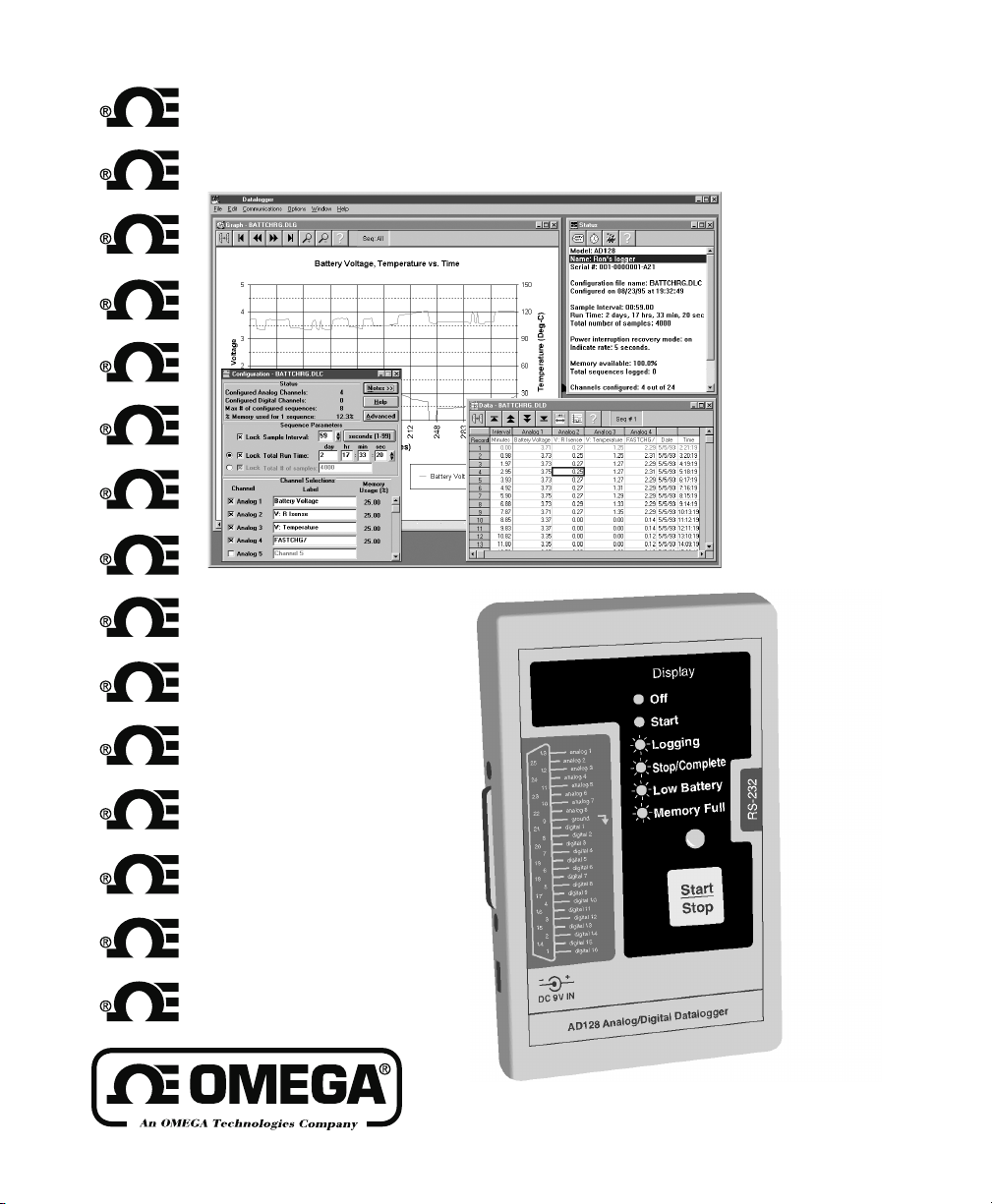
AD128

ANALOG/DIGITAL DATALOGGER

Operators Manual

NLR1195JAC1B

Unpacking Instructions

Remove the Packing List and verify that you have received all equipment, including the following:

• AD128 Datalogger

• MS Windows Application Software Install Disk

• 9-pin to 9-pin Communications Cable*

• Sampling Interface Cable

• AC Adapter

• 9 Volt Battery

• Operator’s Manual

• Storage Box

• 9-pin to 25-pin adapter (if requested)

If you have any questions about the shipment, please call the OMEGA Customer Service Department. When you receive the shipment, inspect the container and equipment for signs of damage. Note any evidence of rough handling in transit. Immediately report any damage to the shipping agent.

NOTES

The carrier will not honor damage claims unless all shipping material is saved for inspection. After examining and removing contents, save packing material and carton in the event reshipment is necessary.

Notes:

Contents

1. GETTING STARTED ............................................................................................7

1.1 UNP ACKING CHECKLIST ..................................................................................7

1.2 SYSTEM REQUIREMENTS ................................................................................. 7

1.3 SOFTWARE INSTALLATION ................................................................................7

1.4 COMMUNICATION SETUP ................................................................................. 8

1.5 QUICKSTART INTRODUCTION ............................................................................8

1.6 QUICKSTART OPERATION DIAGRAM.................................................................. 9

1.7 FEATURE SUMMARY .....................................................................................10

2. OPERATION OVERVIEW.................................................................................11

2.1 STATUS WINDOW .........................................................................................11

2.2 CREATE A CONFIGURATION DOCUMENT.........................................................12

2.2.1 Setting Up The Configuration ............................................ 12

2.2.2 Recommended Procedure ................................................... 13

2.2.3 Channel Selections ............................................................. 14

2.2.4 Sequence Parameters .......................................................... 15

2.2.5 Status Section, Configuration Window .............................. 16

2.2.6 Notes & Advanced Options................................................ 16

2.3 COMMUNICATION .........................................................................................17

2.3.1 Send Configuration............................................................. 17

2.3.2 Receive Data....................................................................... 17

2.4 RECORDING DATA - HARDWARE ....................................................................18

2.4.1 Connecting the Sampling Interface Cable .......................... 18

2.4.2 Datalogger Panel................................................................. 18

2.4.3 Power Supply...................................................................... 19

2.4.4 Start / Stop .......................................................................... 19

2.5 SPREADSHEET DATA VIEW ............................................................................19

2.6 GRAPH DATA VIEW......................................................................................22

3. REFERENCE .......................................................................................................23

3.1 STATUS WINDOW .........................................................................................23

3.2 CONFIGURATION OPTIONS .............................................................................25

5

Contents (continued)

3.2.1 Memory Use ....................................................................... 25

3.2.2 Advanced Configuration Options....................................... 25

3.3 SCALING INPUTS AND DATA .......................................................................... 27

3.3.1 Channel Details ................................................................... 27

3.3.2 Sensors & Scaling Methods................................................ 28

3.3.3 Thermistor Profiles ............................................................. 30

3.4 TRIGGERING, EVENT-BASED RECORDING ....................................................... 31

3.5 SPREADSHEET VIEW FEATURES ..................................................................... 34

3.5.1 Scaling Spreadsheet Data .................................................... 34

3.5.2 Spreadsheet Statistics .......................................................... 34

3.5.3 Printing Spreadsheet Data ................................................... 35

3.5.4 Exporting Spreadsheet Data ............................................... 35

3.6 GRAPH VIEW FEATURES ...............................................................................36

3.6.1 Scaling Graph Data.............................................................. 36

3.6.2 Graph Statistics.................................................................... 37

3.6.3 Printing Graphs.................................................................... 38

3.6.4 Exporting Graphs................................................................. 38

3.6.5 Formatting Graphs ............................................................... 39

3.7 THE AD128 LOGGING UNIT .........................................................................40

APPENDIX A.............................................................................................................42

MODEL AD128 TECHNICAL INFORMATION ...........................................................42

1. Battery Life Vs. Configuration ................................................ 42

2. Timing and Storage Format ..................................................... 43

3. Electrical & Mechanical Specifications................................... 44

4. T arget Interface Pin Designations ............................................ 45

5. Model AD128 Input Circuit Models ....................................... 53

APPENDIX B.............................................................................................................55

LEAD-WIRE COLOR CODE CHART (PIG-TAIL CABLE)............................................55

6

1. GETTING STARTED

1.1 UNPACKING CHECKLIST

Y our Stand-Alone Data Acquisition System package should include the following :

o Model AD128 Logging Unit o AC Adapter o Configuration & Analysis Software CD o 9-Volt Battery o 9-pin Communications Cable o User’s Guide o Sampling Interface Cable o Warranty Registration Card

1.2 SYSTEM REQUIREMENTS

• IBM PC or Compatible, 386 or better

• CD-ROM, CD-R or MultiRead CD Drive

• 8 Mb RAM minimum, 16 Mb recommended

• Windows 95, 98 or newer or Windows NT 4.0 or newer

• 8 Mb available hard disk space

The AD128 system is capable of collecting large amounts of data and presenting the information graphically . Because of this, we recommend that you install the Configuration & Analysis Software on a PC with a fast microprocessor (200Mhz or higher) and as much RAM as possible (16Mb or more).

1.3 SOFTWARE INSTALLATION

Insert the installation disk in the appropriate disk drive, (the following instructions assume that drive D: is your CD drive.)

1. Insert the software CD in your CD drive. The the installation process. If the software driver for your CD drive does not support the autorun function, select

2. Follow the on-screen instructions.

3. To begin, select the C&A program from the the dl32.exe file from the Windows Explorer in the directory where you installed the program (default directory -

Run...

from the

C:\Program Files\C&A

autorun.inf

Start

menu and type in

Start | Programs

)

file will automatically begin

D:\setup

menu, or double-click on

.

7

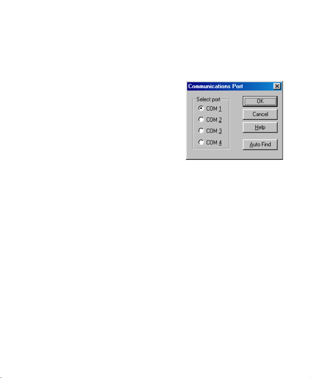
1.4 COMMUNICATION SETUP

From the selection for the PC. Below is the dialog box that appears. Select the correct COM port or use

Auto Find. Auto Find

mode, and it is connected to an available COM port. This will only need to be done once, unless the PC's hardware is changed or a different PC is used.

Most commonly , COM1 or COM2 is used. For notebook computers, almost always COM1 is used, but on some older models, the mouse uses COM1, so you would then use COM2. Rarely is COM3 or COM4 used.

**NOTE: A “Null-Modem” cable is required for communication between the logging unit and the host PC. Only 3 wires are used: TxD, RxD & GND. The wires between pins 2 and 3 (the transmit and receive wires) are crossed in the null-modem configuration. The GND (signal common) is pin 5 on a 9-pin RS-232 connection.

Communication

will find the correct port if the logging unit is powered, but in the “Off”

menu, select

Setup...

to setup or change the communications port

1.5 QUICKSTART INTRODUCTION

The Model AD128 logging unit can sample up to 16 digital and 8 analog channels simultaneously , as fast as 500 times per second or as slow as one time every 99 minutes, with the capacity to store 130,000 readings.

The Configuration & Analysis Software (C&A) was designed to be intuitive, so that you can put this capability to work, right out of the box. The “Quickstart Operation Diagram” in the next section shows you how to do this.

It may be helpful to have this guide open to the Operation Overview, section 2, as you step through the Quickstart Operation Diagram. For this reason, a removable copy of the Quickstart section has been supplied with this User’s Guide. Once you are familiar with the AD128 system you may want to visit the Reference, Section 3, where more advanced features are described, including: Scaling, Event-Based Recording, Formatting, Statistics, Printing and Exporting.

By understanding the basic framework of the AD128 system, you will find that each time you put the system to work, your experience will not be one of constant “relearning”, but one of increasing convenience. A few tips are listed in this introduction and throughout the User’s Guide to help you save even more setup time in future applications.

**Tip: You may use the system for many different applications, or you may use it for the same application every time. In either case, it will be valuable for you to be able to reuse any work you have done in the past. The C&A software gives you the capability to do this by saving configuration files and sensor profiles. Choose meaningful names for configuration files and sensor profiles so that you may make use of them in the future,

8

either for reference or for additional data acquisition tasks. **Tip: Notes can be typed directly into a configuration form for reference. This is an

extremely valuable feature, when utilized: notes, along with ALL configuration settings are stored in data and graph files that are saved to disk. In the same way, all raw data that is retrieved from the logging unit is stored in a graph file. C&A software allows you to recreate a configuration or a complete raw data file, along with scale settings, from a graph file. This capability makes it easy to organize data and assures that you can always duplicate a setup, effortlessly.

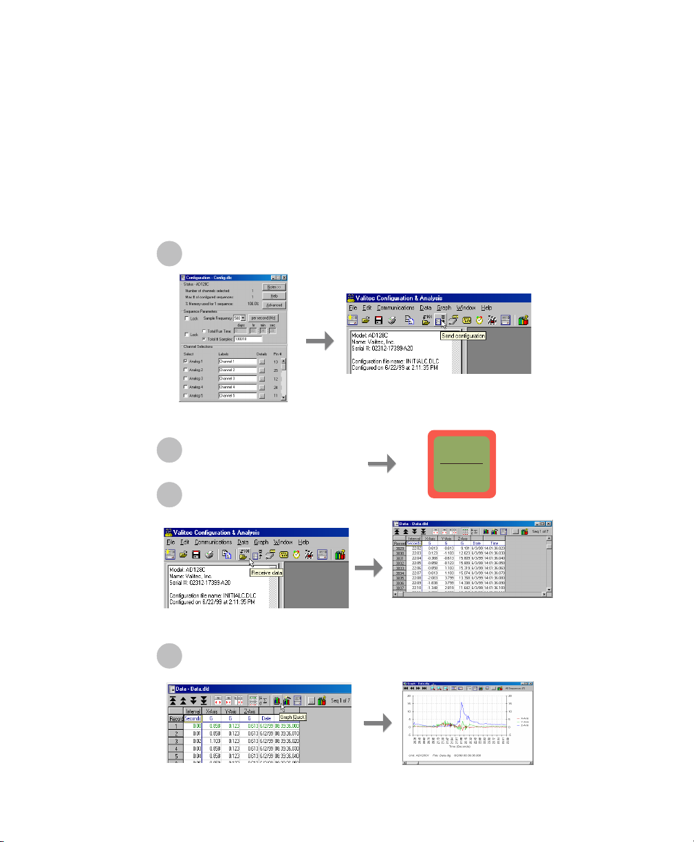
1.6 QUICKSTART OPERATION DIAGRAM

1

Configure (Setup)

Simple form-based configuration

Record Information

2

3

Retrieve Data

Start Stop

Built-in spreadsheet: Graph, Copy/Paste, Print, Export...

4

View Graph

For Analysis or Presentation: Copy/Paste, Print, Export...

9

1.7 FEATURE SUMMARY

Data Acquisition

• Stand-alone operation - uses internal memory to store data

• Interval Recording

• Trigger-based (Event) Recording and Repetitive T riggering

• Status Indication: SAMPLING, TRIGGER-MODE, MEMORY FULL, LOW BATTERY

• Scaling to Engineering Units

• Low-Power, Battery Operation

• 10-year battery backup and software interlock to protect data

Software Framework

• The Configuration & Analysis Software framework is compatible with all AD128 family data acquisition systems, including future models.

• One-button operation to setup the logger, receive data and generate graphs.

• Configurations, data and graphs are treated as documents, much like a word processing document is treated by a word processing program. All information is carried forward to the next level ‘document’, which means that you don’t have to save configurations, data and graphs together as a set - a configuration can be created from an existing data file or graph file; a data file can be created from a graph file. Once a graph is created from data collected by the logging unit, the configuration and data files can be discarded, if desired, for the purpose of storing and organizing data files more efficiently .

• The ‘configuration’ button on the status window allows you to create a configuration ‘document’ from the logging unit that is currently connected to the PC.

Data View & Analysis

• View all data or view only the data acquired from individual recording ‘sequences’.

• Export/Copy data in table or graphical format to file or directly to any other program.

• Print data in table or graphical format.

• Print or copy configuration and status window information. This is useful for documenting collected information.

• Statistics in table and graph views

** The AD128 system is Year 2000 (Y2K) compliant

10

2. OPERATION OVERVIEW

This overview covers the five (5) basic steps involved in collecting and reviewing data. Section 3, titled “Reference”, covers more advanced features, in addition to instructions for reviewing, formatting and exporting in the spreadsheet and graph windows.

Step 1: Create a configuration Step 2: Send a configuration Step 3: Record data Step 4: Receive data Step 5: Generate a graph

2.1 STATUS WINDOW

This window displays the status of a logging unit that is connected to the PC - it is your “window” to the data acquisition hardware. Below is a picture of a logging unit is connected when the Configuration & Analysis program is started, it’s status will be displayed automatically . Other messages relating to the most recent communication with the logging unit will also be displayed here. The display can be updated at any time

Status

window. If a

by selecting the Refresh button on the main progam toolbar.

For more information on the Status window, please go to the Reference section 3.1: “Status Window”.

11

2.2 CREATE A CONFIGURATION DOCUMENT

Before recording information with the logging unit, you must first configure it. This is done by creating a configuration ‘document’ and then sending it to the logging unit. Configuration documents can be created once and saved to disk for reuse in future data collection tasks.

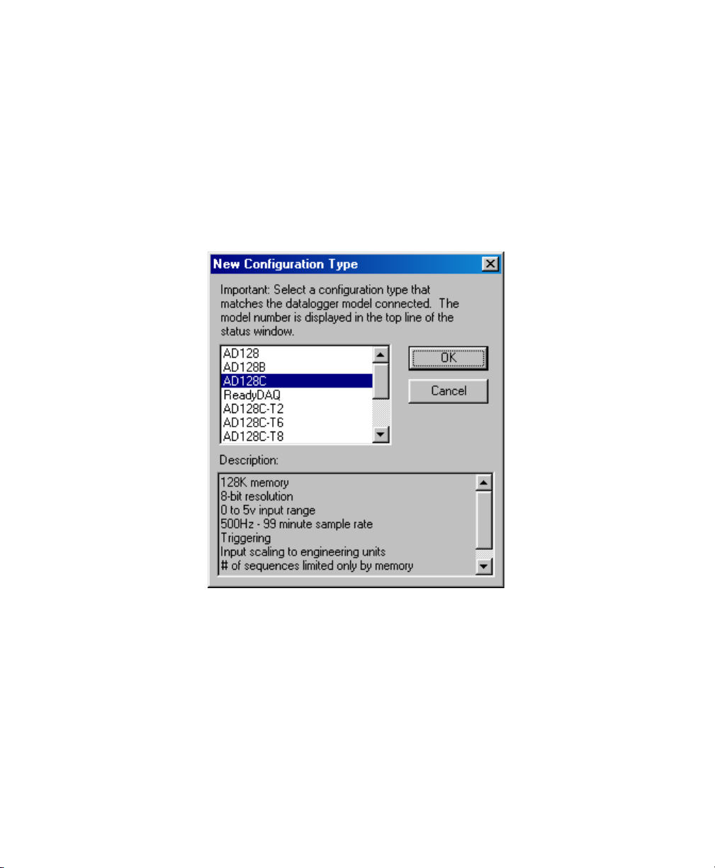
The first step in creating a configuration is to open a New Configuration template by selecting

File | New Configuration...

that matches the target logging unit model. The model number of a logging unit that is connected to the PC’s communication port can be found at the top of the Status window .

from the main menu. Be sure to select the configuration template

File | New Configuration...

Previously saved (to disk) configurations are opened by selecting

NOTE: A configuration document may also be created from a connected logging unit by clicking the configuration button on the main program toolbar. Configurations can be generated directly from data (.dld) and graph (.dlg) files by clicking on the configuration icon on the spreadsheet and graph window toolbars.

File | Open.

2.2.1 Setting Up The Configuration

Recording parameters (sample interval, run time, channel selections, etc.) are established in the configuration. A new configuration is already initialized with everything necessary to begin

12

recording - it can be sent to the logging unit and used, as is. However, you will want to customize the configuration for each task.

The configuration window is a “smart form” that automatically calculates sequence parameters and displays: 1) the fastest Sample Frequency possible, and 2) the Total Run Time that is based on using 100% of the data storage memory available in the target logging unit.

These calculations are updated when you make changes. For example, if you add 3 channels to the default configuration (from 1 to 4), the Total # of Samples and Total Run Time will be reduced by a factor of 4. However, you can “lock in” a Total Run Time by clicking the checkbox next to the Frequency by clicking the

Total Run Time

Lock

checkbox next to that field.

field. Similarly, you can “lock in” a Sample Interval/

Lock

2.2.2 Recommended Procedure

To appreciate the benefits of the “smart form” feature, specify recording parameters in the following order:

1. Select each channel to be sampled and enter meaningful channel names.

2. Set the "Total Run Time" if the test is to be terminated after a specified period of time (though a logging sequence may be interrupted at any time by pressing the "Start/Stop" button on the panel).

Or

Set the "Total # of Samples" if the test is to be terminated automatically after a specified

number of samples have been acquired.

3. Set the "Sample Interval/Frequency" - the time base may be changed by selecting the time base button to the right of the "Sample Interval/Frequency" entry field.

13

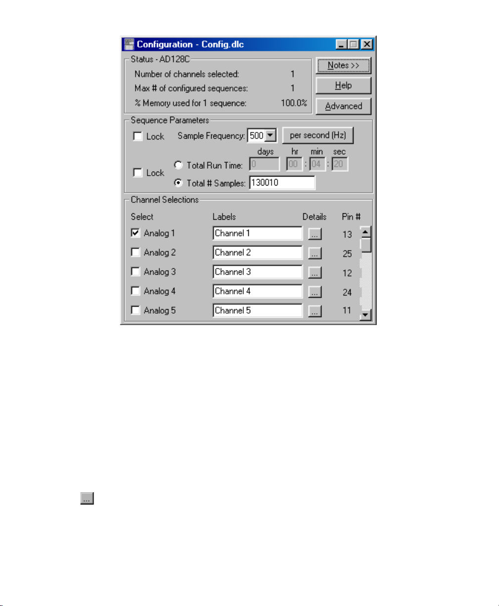
Configuration ‘Document’ Window

2.2.3 Channel Selections

Record

The Model AD128 has 8 analog and 16 digital channels available. Select the channels that will be logged during the recording sequence by clicking on the channel name (Analog 1, Digital 6, etc.). Use the scroll bar on the right to bring other channels into view.

Label

After selecting a channel, the cursor will move to the channel name field. Y ou may enter a meaningful name for each channel, up to 15 characters.

Details

Click on the details button to access more advanced options for the input channels, such as scaling and triggering parameters. For more information regarding scaling and triggering, please go to the reference section titled: Channel Details - Scaling & Triggering.

14

Pin #

The pin number indicated in this field represents the associated pin of the 25-pin D-sub connector on the logging unit.

2.2.4 Sequence Parameters

Sample Interval (/Frequency)

The default sample rate for a New Configuration is 500 Hz (500 samples per second). The sample rate is auto-calculated following entry of other configuration parameters to display the shortest sample interval available.

To set the Sample Interval for a logging sequence, first set the time base by clicking on the time-base button. Next, type in the desired Sample Interval or Frequency .

The Sample Interval field will automatically "lock" when you modify it, disabling automatic calculation of the Sample Interval/Frequency .

NOTE : You may wish to select recording channels and define labels before specifying sequence parameters. This will enable you to see the automatic calculations for total run time and total number of samples.

Total Run Time

The Total Run Time parameter allows you to set the duration of a single logging sequence. To automatically terminate logging after a specified period of time, enter the desired number of days, hours, minutes, and seconds in the respective fields.

Auto-calculation displays the Total Run Time that will result when recording from the selected input channels, at the specified Sample Interval and using all 130,000 data storage locations. When configuration parameters are changed this field is recalculated, unless it is locked. Total Run Time will automatically “lock” if you enter a value in this field, or by clicking in the Lock checkbox. The field may be "unlocked" by deselecting the Lock check box.

If the radio button to the left of the "lock" check box is not selected, the Total Run Time parameter is not enabled. In this case, the Total # of Samples determines the Total Run Time of the sequence, in combination with the Sample Interval.

15

Total Number of Samples

The Total # of Samples parameter lets you to define a logging sequence by the number of samples to be recorded. A sample is defined as a one record of all selected channels. To terminate logging after a specified number of samples have been logged, enter the desired number of samples in this entry field. Manual entry into this field "locks" the Total # of Samples parameter, disabling the auto-calculation feature. The field may be "unlocked" by deselecting the Lock check box.

If the radio button to the left of the "lock" check box is not selected, the Total # of Samples parameter is not enabled. In this case, the Total Run Time determines the number of samples in the configured sequence, in combination with the Sample Interval.

2.2.5 Status Section, Configuration Window

This section indicates the total number of input channels selected for recording. It also displays the percentage of memory required for the configured logging sequence, and the number of sequences of this particular configuration that can be recorded with the available data storage memory .

For more information on memory use, please go to the Reference section 3.2.1: Memory Use.

2.2.6 Notes & Advanced Options

Notes

Select the Notes button to display the "Notes" section of the configuration window. The notes section is convenient for documenting test setup, special equipment, general explanation of intended uses for the configuration and test results information to be kept on file for later use. These notes are saved with the configuration so that whenever the configuration is reloaded from the disk, the test notes will also be available. To view, click the Notes button.

**Tip: This is an extremely valuable feature, when utilized: notes, along with ALL configuration settings are stored in data and graph files that are saved to disk. In the same way, all raw data that is retrieved from the logging unit is stored in a graph file when saved to disk. C&A software allows you to recreate a configuration or a complete raw data file, along with scale settings, from a graph file. This capability makes it easy to organize data and assures that you can always duplicate a setup, effortlessly .

Advanced

(Please see Reference section 3.2.2: Advanced Configuration Options)

16

2.3 COMMUNICATION

The AD128 logging unit must be in the "Off" mode in order to communicate with the Configuration/Analysis Software through a PC serial communications port. Communication codes sent by the PC will "wake up" the logging unit each time communication is initiated. A transfer of information takes place between the PC and logging unit for the following functions:

• Configuration of logging sequence parameters

• Transfer of data to the PC

• Transfer of logging unit status to the PC

• Setting the logging unit's internal clock

• Personalization of the logging unit with a meaningful name

The first of these functions, configuration and data transfer, are initiated by clicking icons on the main program toolbar, or by selecting the appropriate sub-menu item under

Communications

functions may also be accessed from the main menu and toolbar, and are described in the Reference, section 3.1: Status Window.

2.3.1 Send Configuration

NOTE: If data has been logged but not yet received into a data window, this should be done

before re-configuring the logging unit (See section 2.3.2: Receive Data).

on the menu bar; these are described below. The remaining communications

To send a configuration to the logging unit, be sure the unit is not recording (stopped) and is connected to a serial port on the PC with the supplied communications cable. Also make sure that the Configuration window is the “active” window.

From the seconds to send the configuration and to program the logging unit (use the

Setup

Communication Setup). Select "OK" at the warning prompt to proceed. The warning prompt helps to avoid accidental loss of data, as this process overwrites the previous configuration and access to recorded data is lost.

If you have any problems, check to make sure that the Configuration window type (AD128, AD128B, AD128C) matches the logging unit. The logging unit model number appears at the top of the Status window. If you still have problems, recheck the cable connection and verify that your Comm port is set up properly .

Communications

menu option to change ports if necessary - see Getting Started section 1.4:

menu, select

Send Configuration.

It takes approximately 10

Communications |

2.3.2 Receive Data

17

To receive the recorded data, make sure the logging unit is connected to a serial port on the PC with the supplied communications cable. From the

Data

. While data is being transferred, the progress level is displayed on a meter.

If errors occur while attempting to receive data, make sure that the correct COM port is selected (See Getting Started section 1.4: Communication Setup). Also, make sure the cable is securely connected at both ends.

Once the data is received, a variable-size spreadsheet is created, based on channels configured and the number of samples recorded. This is the spreadsheet window, which is specially formatted with the channel names that were specified in the configuration.

Communications

menu, select

Receive

2.4 RECORDING DATA - HARDWARE

This section gives only a brief overview of the AD128 logging unit and it’s use for recording data. For more detailed information, please see the Reference section 3.7: The AD128 Logging Unit, or Appendix A for technical information.

2.4.1 Connecting the Sampling Interface Cable

Connect the 25-conductor cable (included in the shipping package) to the port on the left side of the datalogger. The stripped and tinned leads will connect to the equipment being tested. All leads are color-coded; a chart is provided in Appendix B to assist connection to the respective inputs. Included with the AD128 system is a wallet-size laminated card with the same information for easier use in the field.

2.4.2 Datalogger Panel

The panel of the logging unit includes a color legend for the LED display . This legend describes the operating mode associated with each color displayed by the LED. A flashing display is differentiated from a solid color .

Display

(LED off)

(Green, solid)

(Green, flashing)

(Red, Solid)

(Red, flashing)

(Orange)

18

Off

Start Logging

Stop/Complete Low Battery

Memory Full

* Trigger Mode: The green and orange display flash alternately to indicate that the

logging unit is waiting for the trigger condition to occur.

2.4.3 Power Supply

The AD128 logging unit can be operated with power supply voltages ranging from 7 to 15 volts. A 1 15 VAC / 9 VDC adapter is included with the standard AD128 system. For portable use, alkaline batteries are recommended - typical life curves are based on Duracell alkaline batteries and can be found in Appendix B: Battery Life Vs. Configuration.

Start

2.4.4 Start / Stop

Stop

Press the automatically upon completion, but may be stopped and restarted, manually , by pressing the

Start/Stop

communications.

Start/Stop

button. The logging unit must be in the "off" mode for configuration for

button to begin logging. A configured logging sequence will be terminated

2.5 SPREADSHEET DATA VIEW

This spreadsheet has the same look and feel as popular spreadsheet programs and data is compatible for exporting to any Windows platform spreadsheet or analysis program. For information on scaling, statistics, printing, exporting, and saving spreadsheet files, please go to the Reference section 3.5: Spreadsheet View Features.

19

Example Data Window

All options are available on the right mouse menu and also on the main menu bar under

Options | Data

. Position the mouse over the spreadsheet, click the right mouse button and the

menu will appear. All functions necessary for viewing or exporting are available. To select a range of cells, select

a corner and drag the mouse to the opposite corner. A column or row of cells may be selected by clicking on the column/row header cell.

choices

.

Click the right mouse button to bring up a menu of

Top and Bottom Rows Click these buttons to move to the top or bottom rows of the spreadsheet.

Spreadsheet “Next” and “Previous” Sequence Click these buttons to move the cell cursor to the first row of the next or previous data

sequence. These buttons will have no effect if you are viewing a data file that was recorded in a single sequence.

Column | Auto-Size Use this button to automatically size the selected column(s) to the labels and data in view at a

given time. This is normally not necessary but should be used when viewing the cells in the statistics summary - since the information in these cells is so much wider than is typically in data and label cells, it is sometimes partially hidden to optimize the spreadsheet view.

20

Create Graph A new graph window is generated each time this button is selected. The new graph is a stand-

alone “database” that includes all raw data and configuration information. Refer to the Graph View descriptions in the Operation Overview and Reference sections for more information about graphs generated from the Spreadsheet Data View .

Create Configuration Clicking this button will cause a configuration “document” to be generated from the

Spreadsheet Data View “database”. The spreadsheet has all of the necessary information to construct a duplicate of the original configuration file that was used to record the data.

Data Organization

Data is organized as one row per sample record. Records that represent the time at which recording sequences were started are color-coded green. The last sample record in a sequence is red. All other records are displayed with black text. Each sample record consists of three specific column types: Interval, Sample Data and Time Stamps.

Interval

This column displays the actual time of each sample, starting at 0.0 for each recording sequence and increased by the sample interval value. This column is provided for convenience in creating X-Y charts, as it can be used for "X-range" data.

Sample Data

These columns display sample data read from the specified input channels - one column per selected channel. The user-defined channel label is the column name and the ‘engineering units’ are displayed in the first row. Analog data is displayed as scaled values; by default, 0 to 5 volts. Digital data is displayed as 0 for "off" and 1 for "on". An “on” condition occurs when the input signal exceeds the 3.5 volt threshold of the digital input. This is typically a signal that switches between 0 and 5 volts, but it can be as high as 15 volts.

Time Stamps

The date and time for each data sample are displayed in this column. Data recorded from multiple logging sequences is displayed sequentially . That is, the first data

record in a logging sequence is displayed immediately following the last record of the previous sequence. The start of a new sequence is easily distinguished by the green-colored text, in addition to the 0.0 value in the Interval column.

21

2.6 GRAPH DATA VIEW

V arious formatting options are available on the right mouse menu. Access this menu by placing the mouse over the graph window and clicking the right mouse button.

“All” Sequences Method

Click this toggle button ‘on’ to view all recorded sequences as they were on continuous piece of paper. Each sequence starts right after one another, end-to-end. The x-axis values will reset and count up for each sequence.

When viewing the graph this way , the next and previous sequence buttons have no ef fect. The Graph Start button moves to the beginning of the 1st sequence. The Graph End button moves to the end of the last sequence.

“Individual” Sequence Method

Click this toggle button ‘on’ to view each sequence individually in the graph window. The scroll bar at the bottom will scroll from the beginning of the current sequence to the end of the current sequence. If you want to view other sequences, click the next and previous buttons. The current sequence is displayed on the tool bar.

Graph “Beginning” and “End”

22

Click this button to move the graph view to the beginning of the 1st sequence, regardless of the current graph method. If you are viewing multiple sequences and want to move to the beginning of a particular sequence, use the scroll bar.

Graph “Next” and “Previous” Sequence

Zoom “In” and “Out”

Click this button to zoom in on the data by a factor of 2. The center of the graph window is the zoom point.

Create Spreadsheet

Create Configuration

Use this option to open the configuration form with the parameters used to generate this data. This allows you to quickly configure a logging unit from a previous test file, ensuring that all the options duplicate the original configuration.

3. REFERENCE

3.1 STATUS WINDOW

For general information about the Status window and it’s function, please refer to the Operation Overview, section 2.1: Status Window.

The status of the device currently connected to the communication port is displayed in the status window.

A tool bar is displayed at the top of the main program window. Certain tools on the toolbar are used to communicate with devices connected to the communication port. Clicking the right mouse button while the cursor is over the status window will also bring up the menu of available communication functions.

Name

The logging unit may be personalized for identification. This is especially useful when more than one AD128 is in use for the same or similar applications. The name can have up to 15 characters and may contain any keyboard character.

23

Below is the dialog box that appears when the

Name

button is selected:

The current name is listed at the top. It is also initially placed in the edit field. To change the name, just enter a new name (up to 15 characters) and then press the OK button.

Clock

The logging unit contains a real-time clock. Use this option to change the time and date. The PC's current date and time are the default values placed in the edit fields. To synchronize

the AD128 logging unit's internal clock to the PC, just select "OK". Any other valid setting may be entered, as well. The AD128 system is Y ear 2000 (Y2K) compliant.

Below is the dialog box that appears:

24

NOTE: The time is in 12 hour format (AM or PM must be specified) and the date is month / day / year (2 digit year). This software recognizes the years “00” and up to be the years 2000 and up, so there is no concern for Y2K problems.

Refresh

When the program first starts up, it determines if there is a logging unit connected, and if so, it will display the status. At anytime you can press the Refresh button to get the most up-to-date status of whichever device is connected.

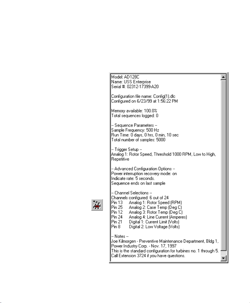
Contents of the Status Window

The Status window is a direct link to the AD128 logging unit. Information displayed here resides in memory within the logging unit, including: date and time of configuration, number and name of input channels selected, configuration parameters and available memory . If there is more information than space provided, scroll bars will appear to permit full viewing.

The status window is updated each time communication is established between the PC and the logging unit.

3.2 CONFIGURATION OPTIONS

3.2.1 Memory Use

Each analog channel requires 1 memory storage location (130,000 storage locations are available for sampled data). Selecting all 8 analog channels would use 8 storage locations each time the inputs are sampled.

The digital channels are read simultaneously in groups of 8: channels 1 through 8 are grouped together, as well as channels 9 through 16. Selecting 1 or more digital channels in the range 1-8 will use 1 storage location for each data sample. Similarly , selecting 1 or more digital channels in the range 9-16 will use 1 storage location. It is most efficient, in terms of memory usage, to select channels within the same group when configuring 8 or less digital signals for logging.

3.2.2 Advanced Configuration Options

Note: Advanced options control the general operation of the logging unit, affecting battery life

and behavior following power interruptions.

25

Advanced Configuration options are accessed from the section of the

Configuration

window.

Advanced

button located in the

Status

Logging Indication Flash Interval

The Logging Indication Flash Interval is the rate at which the Light Emitting Diode (LED) indicator flashes (green) while the logging unit is in the

Logging

mode.

Theory of Operation

Typically, the LED flashes each time a sample is logged; however, if the sample interval is very fast, .05 seconds or less, the LED will stay on constantly while the logging unit is in the logging mode.

With slower sample intervals this method of indication is less useful, as minutes could pass before a flash. For this reason, a method of forcing a "logging indication flash" is provided.

For sample intervals of one (1) second or longer, the LED will flash at a rate which is the faster of the

Sample Interval

or the

Logging Indication Flash Interval

.

For example, if the sample interval is 5 minutes, and the flash interval is 10 seconds, the LED will flash every 10 seconds, even though samples are being logged at 5 minute intervals. The indication is more meaningful if it is frequently visible.

Note : If this value is "0", the LED will not flash at all. Use this option to conserve battery power. Faster flash rates will reduce battery life. The "0" mode functions only when the sample interval is one (1) second or greater. When faster sampling is involved, memory capacity will limit run time, rather than battery life.

Power Interruption Recovery Mode

When this option is selected, logging will resume following a power interruption. If this option

26

is not selected, a loss of power will terminate recording - logging will not resume when the supply voltage returns to the normal operating level.

3.3 SCALING INPUTS AND DATA

3.3.1 Channel Details

“Channel Details” are optional parameters that can be used to further customize an input channel.

Options include scaling the input voltage to engineering units, such as Degrees Celsius, and defining an input or group of inputs as a “trigger”.

The Channel Label can be changed for the input channel that is currently displayed in the Channel field at the top of this window. Any change made here will be reflected in the Configuration window.

The Input Range normally will not change. Select AD128 logging unit. If you purchased the AD128-10, select

0 to 5 volts

0 to 10 volts

if you have the standard Model

. The input range is the

27

basis for scaling calculations and it is important that the correct range is specified. Scaling can be accomplished by applying a defined sensor “profile” to the input channel that is

currently displayed in the Channel field at the top of the Channel Details window. Once this window is displayed, any analog input channel can be scaled by first selecting an input channel and then desired sensor to apply . Click the parameters or to define new sensor profiles. This process is described in the next section:

3.3.2 Sensors & Scaling Methods. Triggering parameters are set in the T rigger Setup window. Bring up this window by clicking

the

T riggering...

Triggering, Event-Based Recording.

button. The trigger setup process is described after the next section in: 3.4

Scaling...

button to review or change scaling

3.3.2 Sensors & Scaling Methods

**IMPORT ANT : Care should be taken in naming, modifying and deleting sensor profiles, as this will affect the interpretation and presentation of preexisting data and graph files that use these sensor profiles. Sensor profiles that have been applied to input channels are indexed by unique sensor names, and changing the scale parameters for these names changes scaling applied wherever they are used. The following paragraphs provide more information related to sensor profile management.

In order to scale an input channel to engineering units, a sensor profile with the desired scale parameters must be applied to that channel. Sensor profiles are created and ‘managed’ in the Scaling window. This window, in combination with the files that store the profiles, form a sensor profile database. This database is ‘managed’ by adding, changing or deleting sensor

28

profiles. A sensor name is used as a reference to identify the scaling equations needed to support scaling an individual sensor output to meaningful units. Once you have entered an equation for scaling, you now only have to reference it by name.

Use the Scaling dialog box to define new scaling equations if the scaling equations you need are not already defined.

For convenience and brevity , sensor profiles will generally be referred to as “sensors”. Two sensor types are available: 1) user-defined sensors that can be created, deleted or

modified, and 2) factory-defined sensors that cannot be modified or deleted. User-defined sensors are preceded by and asterisk ( * ) in the sensor name field, for easy identification.

A sensor cannot be added with the same name as an existing sensor. Each sensor must have a unique name, consisting of at least one different character . Though you may not be recording the output of a sensor at all, the sensor database and management convention provides a way to organize and reuse scaling profiles, trimming keystrokes from future applications.

Add a sensor by typing a unique name in the Sensors: field at the top of the Scaling window, and then click the find it helpful to first select an existing sensor that is similar to the desired new sensor. You should then change the name in the sensor field before modifying scale parameters so that you don’t accidentally “update” the original sensor. However , this will not occur unless you click on the

Update

Add

button, once the desired scale parameters have been entered. You may

button, specifically .

Delete a sensor by making it the currently selected sensor in the Sensors: field, and then click the

Delete

button.

Modify a sensor by making it the currently selected sensor in the Sensor: field. Then, change the scale parameters as needed, and click the

Update

button.

2 Points Scaling Method

To define a scale using the the input signal (volts) to the desired engineering units (i.e. degrees Celsius). You will get the best results by using the 2 known values that are closest to the volts for the standard Model AD128 logging unit).

2 point

method, you may use any 2 known values for converting

Input Range

extremes (0 and 5

Zero-Span Scaling Method

Many sensors are shipped from the manufacturer with scaling information provided in the form of a

Zero

and a

accordingly.

Span

value. To use this method, select

Zero-Span

and fill in the fields

29

Slope/Intercept

Signal or Sensor characteristics may be understood in the form of a line equation, y = mx + b, where ‘m’ is the scaling.

Slope

and ‘b’ is the

Intercept

. Choose

Slope/Intercept

to use this method of

Sensor Database

Sensor database files have the “.sen” extension and are located in the directory where your Configuration & Analysis program is located. Care should be taken so that these files are not damaged or deleted. If you perform regular backups to protect information on your computer you should include these files, but make sure that you are always using the latest version.

3.3.3 Thermistor Profiles

Thermistor sensor profiles can be selected in the usual way that sensor scaling profiles are applied to input channels.

To create new thermistor profiles, the Steinhart-Hart constants are entered in the appropriate fields in the Scaling window, as shown here:

Steinhart-Hart Equation

The Steinhart-Hart equation is an empirical expression that has been determined to be the best mathematical expression for the resistance-temperature relationship of a negative temperature coefficient thermistor . It is usually found explicit in T:

30

1/T = a + b(Ln R) + c(Ln R)^^3 where: T = Kelvin units (deg C + 273.15)

a,b,c = coefficients derived from measurement Ln R = natural logarithm of resistance in ohms

To find a, b and c, measure a thermistor at three temperatures or chose three temperatureresistance pairs from a table provided by the thermistor manufacturer. The temperatures should be evenly spaced, and at least 10 deg C apart. Use the three temperatures and resistances to solve three simultaneous equations:

1/T1 = a + b(Ln R1) + c(Ln R1)^^3 1/T2 = a + b(Ln R2) + c(Ln R2)^^3 1/T3 = a + b(Ln R3) + c(Ln R3)^^3

The equations allow you to derive a, b and c for any temperature range.

3.4 TRIGGERING, EVENT-BASED RECORDING

Enable Trigger

Other than using the Start/Stop button on the logging unit, you can use the trigger mode, causing a recording sequence to begin when a specific “event” occurs. To use this eventbased recording mode, click in the

Enable T rigger

checkbox.

31

Trigger Setup Window

Several types of events can be used to trigger a recording sequence. To choose the method that applies to your application, select an option from the

T ype

field.

Analog

The

Analog

option allows you to trigger recording when an analog input exceeds a specified threshold. In addition, you can specify the trigger to occur when the signal is increasing or decreasing when it crosses the threshold. Behavior is similar to the trigger feature of most oscilloscopes.

Analog (Multiple)

This

Multiple Analog

trigger method will cause the trigger to occur when any of the inputs from Analog Channels 1, 2 and 3 meets the threshold and polarity criteria. A 3-axis accelerometer application is an example of a situation that might call for this method of triggering. When any of the 3 axes exceed a specified shock threshold, recording will begin.

Digital

Select the

Digital

trigger method to trigger when a digital input transitions from “high/on” to

“low/off” or the reverse.

State Change

You can use the

32

State Change

method to trigger when any one of the 16 digital inputs changes

state, say when a switch goes from “open” to “closed”. Any unused digital inputs must be terminated to either ground or 5 volts, depending on the state that you specify . This feature is useful for monitoring a process or troubleshooting a control system.

State Match

The

State Match

when all digital inputs

method is similar to State Change, except that the trigger will occur only

match

the specified levels.

Single Sequence / Repetitive

Select

Single Sequence

triggering to record every time the event occurs, indefinitely , or until memory is full. Each trigger method requires that the trigger is first “cocked”. That is, in order for the trigger

condition to occur, the inputs must first be in a state other than the trigger condition. In order to trigger when a state match occurs, the inputs must first be in a non-matching state specifically , for at a time period of at least 1 millisecond (0.001 second). This is partly to avoid

Repetitive

psi, it must first be below 100 psi.

triggering during the same “event”. To trigger when an analog input rises above 100

to record only at the first occurrence of the event. Use

Repetitive

Trigger Channel

The

T rigger Channel

analog or digital channel to be the trigger input. This field is not used for State Match or State Change trigger methods.

does not have to be an input that is selected for recording. Select any

Sensor

The trigger input can be scaled. Use a sensor from the sensor database to define the scale and then specify the threshold in terms of the scale for that sensor. If a compatible sensor is not available, the sensor must first be created. This can be done from within the Channel Details box. You can get to the Channel Details box from the Configuration window. The

Sensor

field only applies with the Analog trigger method.

Threshold

Specify the desired threshold for the trigger event to occur. The valid range and units are displayed to the right of this field. The

Threshold

field only applies to analog trigger methods.

Low to High, High to Low

Select the polarity of the trigger event here. This parameter does not apply to

State

triggering.

State Match / State Change

Fill these fields with the desired trigger state. “1’s” represent a 5 volt, or “high” signal at the input of the corresponding input. “0’s” represent a 0 volt, or “low” signal, accordingly.

33

3.5 SPREADSHEET VIEW FEATURES

For general information on using the Spreadsheet View , please refer to Section 2.5: Spreadsheet Data View , in the Operation Overview. Additional features are described here that relate to formatting, analyzing, printing and exporting of spreadsheet data.

All options are available on the right mouse menu and also on the main menu bar under Options | Data. Position the mouse over the spreadsheet, click the right mouse button and the menu will appear.

3.5.1 Scaling Spreadsheet Data

Data records that appear in the Spreadsheet window can be scaled in the same way as the logging unit input channels are scaled prior to recording data. Each column of data is treated as a “channel” and scaled as described in Section 3.3: Scaling Inputs & Data. The Channel Details window contains only the fields that apply to the Spreadsheet View , but has a similar format as when selected from the Configuration window.

3.5.2 Spreadsheet Statistics

34

A statistical summary of data recorded from each input channel is displayed at the bottom of the spreadsheet. The statistical quantities include: Minimum, Maximum, Average (Mean), Standard Deviation-Sample, and Standard Deviation-Population. The statistical summary applies to all data in the current “sheet” for the associated channel column.

3.5.3 Printing Spreadsheet Data

Highlight the desired cells, and select available for printing the entire spreadsheet, in color, border, gridlines and for setting page margins. Printing the entire spreadsheet includes the statistical summary and the channel names and labels.

File

|

Print...

from the menu bar. Additional options are

3.5.4 Exporting Spreadsheet Data

Data can be exported using either of two methods:

Method 1 - Copy Directly to Another Program

Highlight the desired cells, and select mouse button pop-up menu (or Control C). In the application to which the information is to be copied, select

**The entire spreadsheet can be highlighted by clicking in the top left cell in the spreadsheet (just to the left of the “Interval” label). The statistical summary is included when you do this, as are all of the channel names and labels.

Paste

from the edit menu (or Control V).

Method 2 - Export as an ASCII File

Edit

|

Copy

from the menu bar or

Copy

from the right

35

Select name with a ".txt" extension and click on "OK". Select a column delimiter - Comma, Space or Tab.

File

|

Save As...

from the menu bar. In the

File Type

field, choose *.txt. Enter a file

3.6 GRAPH VIEW FEATURES

For general information on using the Graph View , please refer to Section 2.6: Graph Data View , in the Operation Overview. Additional features are described here that relate to formatting, analyzing, printing and exporting of graph data.

**Note: The graph view offers presentation quality output for copying and printing - in color or black ink - but can be significantly degraded by the limited resolution of most monitors and graphics controllers. Though the display may look poor, especially when viewing 3D graphs, the output will be crisp.

Selected, commonly used features are described in this section, but many powerful presentation features are available and can be discovered by exploring the options with a real data file. All formatting options are available on the right mouse menu (click the right mouse button and the menu will appear) and also on the main menu bar under Options | Graph. Several features are worth noting, such as 3D plotting and rotating, placing images on a graph, adding background colors and gradients.

**Tip: to rotate a 3D graph, hold down Control+Shift, click the left mouse button wherever you want a “handle” on the graph, and then drag the mouse.

3.6.1 Scaling Graph Data

Data records that appear in the Graph window can be scaled in the same way as the logging unit input channels are scaled prior to recording data. Each data series is treated as a

36

“channel” and scaled as described in Section 3.3: Scaling Inputs & Data. The Channel Details window contains only the fields that apply to the Graph View , but has a similar format as when selected from the Configuration window.

3.6.2 Graph Statistics

A graphic representation of a statistical summary can be applied to any data series, or “channel”. The statistical quantities available are: Minimum, Maximum, Mean (Average), Standard Deviation and Regression (“best-fit” linear approximation). These statistical quantities apply to the data that is currently in view.

The Statistics options can be accessed by double-clicking on the data series for which you want to apply the statistic formula, or by clicking the right mouse button and selecting Series, Series..., and then the desired channel (series) name. The Statistics tab will then be available, as shown in the dialog box above. The result of Minimum, Maximum and Mean applied to a data series is shown in the graph below.

37

3.6.3 Printing Graphs

Make sure the graph window is active, and select available on the Print dialog box for: 1) layout, and 2) fitting the graph to the paper. The default options have been set to those that are most widely used, and generally give good results.

**Tip: Do not resize the “plot” area of the graph by dragging the mouse. This indicates a manual “fix” of the graph size and disables optimal scaling of the graph to the printer page size. If you wish to enlarge the graph for viewing on the screen, try maximizing the graph window, first.

Additional options are available for centering the graph on the printer page and setting page margins.

File

|

Print...

from the menu bar. Options are

3.6.4 Exporting Graphs

Graphs can be exported using either of two methods:

38

Method 1 - Copy Directly to Another Program

Make sure the graph window is active, and select the right mouse button pop-up menu (or Control C). In the application to which the information is to be copied, select

**Many programs offer options for pasting, usually if you select Edit | Paste Special... in the target program before pasting. The Configuration & Analysis program exports the graph in two formats that may be used by any other program, metafile is generally preferred when you wish to be able to resize the image and retain high quality fonts and graphic components, since it is vector-based. Bitmaps allow for editing images at the pixel level, and can be used in programs that do not accept vectorbased images

Paste

from the edit menu (or Control V).

Edit

|

Copy

from the menu bar or

Metafile

and

Bitmap

Copy

. The

from

Method 2 - Save as an Image File

Select

File

|

Save As...

Enter a file name with the appropriate extension and click on "OK".

from the menu bar. In the

File Type

field, choose Metafile or Bitmap.

3.6.5 Formatting Graphs

Most graph objects (axis scale, data series, footnote, titles) can be formatted by doubleclicking on the object.

Some useful, but not-so-obvious, features and methods are described here to get you started.

Format Chart Options

Position the mouse over the graph window and click the right button. Select Options in the Chart Designer include the display format for the title, footnote, legend and second Y axis on the current chart. From tree view in the left panel of this dialog you can also format any other feature of the chart.

Chart Designer....

Plot On 2nd Y Axis

When viewing more than one data series and the magnitude of the scaled data differs greatly, one signal may be “in the dirt” or out of view, depending on how the Y axis is scaled. It may be helpful to plot one or more data series’ on the 2nd Y axis, so that two scales can be used. To do this, double-click on any data series to pop up the Chart Designer with the Options tab selected for that particular data series. Then select

Plot On 2nd Y Axis

.

Format Axis / Scale

To change the scale of an axis, double-click on the axis to pop up the Chart Designer with the Scale tab selected for that particular axis.

39

3.7 THE AD128 LOGGING UNIT

The panel of the logging unit includes a color legend for the LED display . This legend describes the operating mode associated with each color displayed by the LED. A flashing display is differentiated from a solid color .

OFF No display - the logging unit is currently idle.

START

Green, momentary - a logging sequence has been initiated from the "Start/Stop" button on the panel.

LOGGING

Green, flashing - currently sampling (See section 3.2.2: Advanced Configuration Options, for more information).

STOP/COMPLETE

Red, momentary - a configured logging sequence has run to completion or the current sequence has been "Stopped" manually from the "Start/Stop" button on the panel.

LOW BA TTERY

Red, flashing, 1/2 Hz for 10 seconds - low battery; change immediately . The logging unit is always operating when a battery is installed. Even a "dead" battery will provide enough power

40

for subsystems to operate, allowing notification of the low battery voltage condition for some time. A sufficiently discharged battery may not give the full 10-second indication. Data memory is protected by a separate built-in lithium battery . Following replacement of the primary alkaline battery , the current logging sequence may be continued. Loss of power has the same effect as pressing the "Start/Stop" button on the panel, with the exception of Power Interruption Recovery Mode (see Section 3.2.2: Advanced Configuration Options).

MEMORY FULL

Data and time/date stamp memory is full - transfer data and re-configure (configuring has the effect of resetting memory; access to logged data is lost).

Display

Off

Start Logging

13 -------- analog 1

25 ----- analog 2

12 -------- analog 3

24 ----- analog 4

11 -------- analog 5

23 ----- analog 6

10 -------- analog 7

22 ----- analog 8

9 -------- ground

21 ----- digital 1

8 -------- digital 2

20 ----- digital 3

7 -------- digital 4

19 ----- digital 5

6 -------- digital 6

18 ----- digital 7

5 -------- digital 8

17 ----- digital 9

4 -------- digital 10

16 ----- digital 11

3 -------- digital 12

15 ----- digital 13

2 -------- digital 14

14 ----- digital 15

1 -------- digital 16

Stop/Complete Low Battery

Memory Full

RS-232

Start Stop

-

+

DC 9V IN

AD128 Analog/Digital Datalogger

41

APPENDIX A

MODEL AD128 TECHNICAL INFORMATION

1. Battery Life Vs. Configuration

Battery life is virtually Independent of the number of channels configured for sampling; remember that with 1 channel selected, 130,000 samples records can be logged. With 4 analog channels selected, 32,500 records will consume all 130,000 available storage locations.

For short run times, power consumption is not critical. However, with long run times in applications which require battery operation, it is important to verify that the configuration will run to completion before the battery is drained.

The following graph shows the effect of variations in the various

The

Sample Intervals

Sample Interval

at room temperature.

Battery Life Vs Flash I nterva l

(for Various S am p l e Intervals )

60

50

30 seconds

40

30

20

Battery Life (Days)

10

5 seconds

1 second

0

0 102030405060

Duracell Alkaline Battery Life, Full Capacity

10 seconds

20 seconds

Select up to 20 second indication interval from "Advanced" options in "Configuration" window.

If "0" is selected, indication is disabled, resulting in best battery life.

Flash Interval

directly affects battery life; each sample recorded consumes a fixed

Logging Indication Flash Interval

10 minutes 2 minutes

1 minute

with

amount of power. To be sure a logging sequence will run to completion before battery power is expired, find the desired logging sequence

Total Run Time

on the "Battery Life (Days)" axis on this chart. A horizontal line drawn through this point will intersect the curves for various Sample Intervals, indicating valid combinations of the sampling and flash intervals for which a

42

Duracell Alkaline battery , at full capacity, will provide proper operation.

**IMPORT ANT: This profile for battery life does not apply when the is enabled. With trigger mode enabled, battery life is much shorter . The actual life is not be specified because of the many options and unknown trigger frequency . Estimated operating time for a 9V alkaline cell ranges between 15 and 30 hours in the trigger mode.

Trigger Mode

External Battery

To determine the external battery capacity requirement for use in remote applications, first use a current meter in series with any power source to measure the current draw while running the logging unit in the desired operating hours. This gives the approximate “amp-hour” requirement that can be used to select an appropriate battery . It is a good idea to allow at least 20% surplus capacity when sizing batteries. For example, if the measured current is 25mA and application requires operation for one 8-hour session, 200mA-hrs capacity is required; a standard 9V alkaline battery with over 500mA capacity would be sufficient.

Another example: a six-pack of standard 15,000mA-hr “D” cells at 80% capacity will give 480 hours, or 20 continuous days of service with a 25mA draw.

Note: Use of a 9V Lithium battery will more than double battery life, compared to a standard alkaline cell.

T rigger Mode

. Then multiply the measured current value by the number of

2. Timing and Storage Format

The sequence in which input channels are sampled follows the order shown in the application software configuration window, starting with Analog 1 (Channel 1) and ending with Digital 16 (Channel 24).

Each analog channel to be sampled requires approximately 200 microseconds. Actual sampling is completed after 12 microseconds (this is the "sampling time aperture"); however, some time is required for conversion and filtering. Four (4) of these samples are taken and then averaged for each reading to be recorded.

Digital channels are recorded after all configured analog channels have been sampled. Readings of digital channels 1 through 8 occur simultaneously . Digital channels 9 through 16 are also read simultaneously .

43

3. Electrical & Mechanical Specifications

INPUTS 8 analog, 16 digital (except X, -T models)

Analog

Input Voltage Range 0 to 5 V (AD128-10: 0 to 10V) Resolution 20mV (AD128-10: 40mV) Absolute Accuracy ± 10mV (AD128-10: ±20mV) Input Bias Current 400 nA (AD128-10: ~15kW)

Digital

"Going High" Threshold 3.5 V (Maximum) "Going Low" Threshold 1.0 V (Minimum)

Input Bias Current ± 10 mA Connector Type Standard DB 25-pin Sampling Frequency Fast as 500 Hz, Slow as 99 min.

(all channels)

DATA STORAGE

Data Storage 130,000 samples Recording Duration 0.002 seconds to years Data Memory Battery Life 10 years

OPERATING

Power Supply

Voltage 7 to 12 volts (9V batt. / Adapt.)

Current

Standby 300mA

Recording 4mA (only while sampling)

LED Indication (sampling) 10mA (can be disabled) Battery Life Up to 3 months, 9V Alkaline

(Up to 6 months, lithium)

Power Adapter (included) 110V-9V 200mA AC adapter Temperature

Operating 0 to 50 degrees Celsius

Storage -20 to +70 degrees Celsius

44

COMMUNICATION

RS-232 Interface

Baud Rate 9600 bps

Connection 9-pin female

Data Format 8 data, no parity, 1 stop bit

DIMENSIONS 5.8" x 3.6" x 1.3"

(14.7cm x 9.14cm x 3.3cm)

WEIGHT 8 oz. (226 g)

4. Target Interface Pin Designations

4.1 AD128C Connection Diagram

Pin Description Application Wiring

13

--------------------- Analog 1

25

--------------------------- Analog 2 12

--------------------- Analog 3

24

--------------------------- Analog 4 11

--------------------- Analog 5

23

--------------------------- Analog 6 10

--------------------- Analog 7

22

--------------------------- Analog 8 9

--------------------- Signal Common

21

--------------------------- Digital 1 8

--------------------- Digital 2

20

--------------------------- Digital 3 7

--------------------- Digital 4

19

--------------------------- Digital 5 6

--------------------- Digital 6

18

--------------------------- Digital 7 5

--------------------- Digital 8

17

--------------------------- Digital 9 4

--------------------- Digital 10

16

--------------------------- Digital 11 3

--------------------- Digital 12

15

--------------------------- Digital 13 2

--------------------- Digital 14

14

--------------------------- Digital 15 1

--------------------- Digital 16

-----------------------------------

----------------------------

------------------------------------

----------------------------------

Analog 0 to 5 volts Analog 0 to 5 volts Analog 0 to 5 volts Analog 0 to 5 volts Analog 0 to 5 volts Analog 0 to 5 volts Analog 0 to 5 volts Analog 0 to 5 volts Common Ground Discrete Signal, 3.5V high / 1.0V low thresholds Discrete Signal, 3.5V high / 1.0V low thresholds Discrete Signal, 3.5V high / 1.0V low thresholds Discrete Signal, 3.5V high / 1.0V low thresholds Discrete Signal, 3.5V high / 1.0V low thresholds Discrete Signal, 3.5V high / 1.0V low thresholds Discrete Signal, 3.5V high / 1.0V low thresholds Discrete Signal, 3.5V high / 1.0V low thresholds Discrete Signal, 3.5V high / 1.0V low thresholds Discrete Signal, 3.5V high / 1.0V low thresholds Discrete Signal, 3.5V high / 1.0V low thresholds Discrete Signal, 3.5V high / 1.0V low thresholds Discrete Signal, 3.5V high / 1.0V low thresholds Discrete Signal, 3.5V high / 1.0V low thresholds Discrete Signal, 3.5V high / 1.0V low thresholds Discrete Signal, 3.5V high / 1.0V low thresholds

45

4.2 AD128C-2.5 Connection Diagram

Pin Description Application Wiring

13

--------------------- Analog 1

25

--------------------------- Analog 2 12

--------------------- Analog 3

24

--------------------------- Analog 4 11

--------------------- Analog 5

23

--------------------------- Analog 6 10

--------------------- Analog 7

22

--------------------------- Analog 8 9

--------------------- Signal Common

21

--------------------------- Digital 1 8

--------------------- Digital 2

20

--------------------------- Digital 3 7

--------------------- Digital 4

19

--------------------------- Digital 5 6

--------------------- Digital 6

18

--------------------------- Digital 7 5

--------------------- Digital 8

17

--------------------------- Digital 9 4

--------------------- Digital 10

16

--------------------------- Digital 11 3

--------------------- Digital 12

15

--------------------------- Digital 13 2

--------------------- Digital 14

14

--------------------------- Digital 15 1

--------------------- Digital 16

-----------------------------------

-------------------------------

------------------------------

----------------------------

------------------------------------

----------------------------------

-------------------------

Analog 0 to 2.5 volts Analog 0 to 2.5 volts Analog 0 to 2.5 volts Analog 0 to 2.5 volts Analog 0 to 2.5 volts Analog 0 to 2.5 volts Analog 0 to 2.5 volts Analog 0 to 2.5 volts Common Ground Discrete Signal, 3.5V high / 1.0V low thresholds Discrete Signal, 3.5V high / 1.0V low thresholds Discrete Signal, 3.5V high / 1.0V low thresholds Discrete Signal, 3.5V high / 1.0V low thresholds Discrete Signal, 3.5V high / 1.0V low thresholds Discrete Signal, 3.5V high / 1.0V low thresholds Discrete Signal, 3.5V high / 1.0V low thresholds Discrete Signal, 3.5V high / 1.0V low thresholds Discrete Signal, 3.5V high / 1.0V low thresholds Discrete Signal, 3.5V high / 1.0V low thresholds Discrete Signal, 3.5V high / 1.0V low thresholds Discrete Signal, 3.5V high / 1.0V low thresholds Discrete Signal, 3.5V high / 1.0V low thresholds Discrete Signal, 3.5V high / 1.0V low thresholds Discrete Signal, 3.5V high / 1.0V low thresholds Discrete Signal, 3.5V high / 1.0V low thresholds

46

4.3 AD128C-T2 Connection Diagram

Pin Description Application Wiring

13

--------------------- Analog 1

25

--------------------------- Analog 2 12

--------------------- Analog 3

24

--------------------------- Analog 4 11

--------------------- Analog 5

23

--------------------------- Analog 6 10

--------------------- Thermistor 1

22

--------------------------- Thermistor 2 9

--------------------- Signal Common

21

--------------------------- Digital 1 8

--------------------- Digital 2

20

--------------------------- Digital 3 7

--------------------- Digital 4

19

--------------------------- Digital 5 6

--------------------- Digital 6

18

--------------------------- Digital 7 5

--------------------- Digital 8

17

--------------------------- Digital 9 4

--------------------- Digital 10

16

--------------------------- Digital 11 3

--------------------- Digital 12

15

--------------------------- Digital 13 2

--------------------- Digital 14

14

--------------------------- Thermistor Drive 1

--------------------- Thermistor Drive

-----------------------------------

-------------------------------

------------------------------

----------------------------

------------------------------------

----------------------------------

-------------------------

Analog 0 to 5 volts Analog 0 to 5 volts Analog 0 to 5 volts Analog 0 to 5 volts Analog 0 to 5 volts Analog 0 to 5 volts One wire of Thermistor 1 One wire of Thermistor 2 Common Ground Discrete Signal, 3.5V high / 1.0V low thresholds Discrete Signal, 3.5V high / 1.0V low thresholds Discrete Signal, 3.5V high / 1.0V low thresholds Discrete Signal, 3.5V high / 1.0V low thresholds Discrete Signal, 3.5V high / 1.0V low thresholds Discrete Signal, 3.5V high / 1.0V low thresholds Discrete Signal, 3.5V high / 1.0V low thresholds Discrete Signal, 3.5V high / 1.0V low thresholds Discrete Signal, 3.5V high / 1.0V low thresholds Discrete Signal, 3.5V high / 1.0V low thresholds Discrete Signal, 3.5V high / 1.0V low thresholds Discrete Signal, 3.5V high / 1.0V low thresholds Discrete Signal, 3.5V high / 1.0V low thresholds Discrete Signal, 3.5V high / 1.0V low thresholds Second wire of Thermistor 1 Second wire of Thermistor 2

47

4.4 AD128C-T6/10T6* Connection Diagram

Pin Description Application Wiring

13

--------------------- Analog 1

25

--------------------------- Analog 2 12

--------------------- Thermistor 1

24

--------------------------- Thermistor 2 11

--------------------- Thermistor 3

23

--------------------------- Thermistor 4 10

--------------------- Thermistor 5

22

--------------------------- Thermistor 6 9

--------------------- Signal Common

21

--------------------------- Digital 1 8

--------------------- Digital 2

20

--------------------------- Digital 3 7

--------------------- Digital 4

19

--------------------------- Digital 5 6

--------------------- Digital 6

18

--------------------------- Digital 7 5

--------------------- Digital 8

17

--------------------------- Digital 9 4

--------------------- Digital 10

16

--------------------------- Thermistor Drive 3

--------------------- Thermistor Drive

15

--------------------------- Thermistor Drive 2

--------------------- Thermistor Drive

14

--------------------------- Thermistor Drive 1

--------------------- Thermistor Drive

-----------------------------------

-------------------------------

------------------------------

----------------------------

------------------------------------

----------------------------------

-------------------------

Analog 0 to 5/10 volts* Analog 0 to 5/10 volts* One wire of Thermistor 1 One wire of Thermistor 2 One wire of Thermistor 3 One wire of Thermistor 4 One wire of Thermistor 5 One wire of Thermistor 6 Common Ground Discrete Signal, 3.5V high / 1.0V low thresholds Discrete Signal, 3.5V high / 1.0V low thresholds Discrete Signal, 3.5V high / 1.0V low thresholds Discrete Signal, 3.5V high / 1.0V low thresholds Discrete Signal, 3.5V high / 1.0V low thresholds Discrete Signal, 3.5V high / 1.0V low thresholds Discrete Signal, 3.5V high / 1.0V low thresholds Discrete Signal, 3.5V high / 1.0V low thresholds Discrete Signal, 3.5V high / 1.0V low thresholds Discrete Signal, 3.5V high / 1.0V low thresholds Second wire of Thermistor 1 Second wire of Thermistor 2 Second wire of Thermistor 3 Second wire of Thermistor 4 Second wire of Thermistor 5 Second wire of Thermistor 6

* For -10T6 version, Analog 1 and Analog 2 have 0 to 10V input range

48

4.5 AD128C-T8 Connection Diagram

Pin Description Application Wiring

13

--------------------- Thermistor 1

25

--------------------------- Thermistor 2 12

--------------------- Thermistor 3

24

--------------------------- Thermistor 4 11

--------------------- Thermistor 5

23

--------------------------- Thermistor 6 10

--------------------- Thermistor 7

22

--------------------------- Thermistor 8 9

--------------------- Signal Common

21

--------------------------- Digital 1 8

--------------------- Digital 2

20

--------------------------- Digital 3 7

--------------------- Digital 4

19

--------------------------- Digital 5 6

--------------------- Digital 6

18

--------------------------- Digital 7 5

--------------------- Digital 8

17

--------------------------- Thermistor Drive 4

--------------------- Thermistor Drive

16

--------------------------- Thermistor Drive 3

--------------------- Thermistor Drive

15

--------------------------- Thermistor Drive 2

--------------------- Thermistor Drive

14

--------------------------- Thermistor Drive 1

--------------------- Thermistor Drive

-----------------------------------

-------------------------------

------------------------------

----------------------------

------------------------------------

----------------------------------

-------------------------

One wire of Thermistor 1 One wire of Thermistor 2 One wire of Thermistor 3 One wire of Thermistor 4 One wire of Thermistor 5 One wire of Thermistor 6 One wire of Thermistor 7 One wire of Thermistor 8 Common Ground Discrete Signal, 3.5V high / 1.0V low thresholds Discrete Signal, 3.5V high / 1.0V low thresholds Discrete Signal, 3.5V high / 1.0V low thresholds Discrete Signal, 3.5V high / 1.0V low thresholds Discrete Signal, 3.5V high / 1.0V low thresholds Discrete Signal, 3.5V high / 1.0V low thresholds Discrete Signal, 3.5V high / 1.0V low thresholds Discrete Signal, 3.5V high / 1.0V low thresholds Second wire of Thermistor 1 Second wire of Thermistor 2 Second wire of Thermistor 3 Second wire of Thermistor 4 Second wire of Thermistor 5 Second wire of Thermistor 6 Second wire of Thermistor 7 Second wire of Thermistor 8

49

4.6 AD128C-10T2 Connection Diagram

Pin Description Application Wiring

13

--------------------- Analog 1

25

--------------------------- Analog 2 12

--------------------- Analog 3

24

--------------------------- Analog 4 11

--------------------- Analog 5

23

--------------------------- Analog 6 10

--------------------- Thermistor 1

22

--------------------------- Thermistor 2 9

--------------------- Signal Common

21

--------------------------- Digital 1 8

--------------------- Digital 2

20

--------------------------- Digital 3 7

--------------------- Digital 4

19

--------------------------- Digital 5 6

--------------------- Digital 6

18

--------------------------- Digital 7 5

--------------------- Digital 8

17

--------------------------- Digital 9 4

--------------------- Digital 10

16

--------------------------- Digital 11 3

--------------------- Digital 12

15

--------------------------- Digital 13 2

--------------------- Digital 14

14

--------------------------- Thermistor Drive 1

--------------------- Thermistor Drive

-----------------------------------

-------------------------------

------------------------------

----------------------------

------------------------------------

----------------------------------

-------------------------

Analog 0 to 10 volts Analog 0 to 10 volts Analog 0 to 10 volts Analog 0 to 10 volts Analog 0 to 10 volts Analog 0 to 10 volts One wire of Thermistor 1 One wire of Thermistor 2 Common Ground Discrete Signal, 3.5V high / 1.0V low thresholds Discrete Signal, 3.5V high / 1.0V low thresholds Discrete Signal, 3.5V high / 1.0V low thresholds Discrete Signal, 3.5V high / 1.0V low thresholds Discrete Signal, 3.5V high / 1.0V low thresholds Discrete Signal, 3.5V high / 1.0V low thresholds Discrete Signal, 3.5V high / 1.0V low thresholds Discrete Signal, 3.5V high / 1.0V low thresholds Discrete Signal, 3.5V high / 1.0V low thresholds Discrete Signal, 3.5V high / 1.0V low thresholds Discrete Signal, 3.5V high / 1.0V low thresholds Discrete Signal, 3.5V high / 1.0V low thresholds Discrete Signal, 3.5V high / 1.0V low thresholds Discrete Signal, 3.5V high / 1.0V low thresholds Second wire of Thermistor 1 Second wire of Thermistor 2

50

4.7 AD128CX Connection Diagram

Pin Description Application Wiring

13

--------------------- Analog 1

25

--------------------------- Analog 2 12

--------------------- Analog 3

24

--------------------------- Analog 4 11

--------------------- Analog 5

23

--------------------------- Analog 6 10

--------------------- Analog 7

22

--------------------------- Analog 8 9

--------------------- Signal Common

21

--------------------------- Digital 1 8

--------------------- Digital 2

20

--------------------------- Digital 3 7

--------------------- Digital 4

19

--------------------------- Digital 5 6

--------------------- Digital 6

18

--------------------------- Digital 7 5

--------------------- Digital 8

17

--------------------------- Digital 9 4

--------------------- Digital 10

16

--------------------------- Digital 11 3

--------------------- Digital 12

15

--------------------------- Digital 13 2

--------------------- Digital 14

14

--------------------------- Sensor Ground 1

--------------------- Sensor Power

-----------------------------------

----------------------------

------------------------------------

----------------------------------

Analog 0 to 5 volts Analog 0 to 5 volts Analog 0 to 5 volts Analog 0 to 5 volts Analog 0 to 5 volts Analog 0 to 5 volts Analog 0 to 5 volts Analog 0 to 5 volts Common Ground Discrete Signal, 3.5V high / 1.0V low thresholds Discrete Signal, 3.5V high / 1.0V low thresholds Discrete Signal, 3.5V high / 1.0V low thresholds Discrete Signal, 3.5V high / 1.0V low thresholds Discrete Signal, 3.5V high / 1.0V low thresholds Discrete Signal, 3.5V high / 1.0V low thresholds Discrete Signal, 3.5V high / 1.0V low thresholds Discrete Signal, 3.5V high / 1.0V low thresholds Discrete Signal, 3.5V high / 1.0V low thresholds Discrete Signal, 3.5V high / 1.0V low thresholds Discrete Signal, 3.5V high / 1.0V low thresholds Discrete Signal, 3.5V high / 1.0V low thresholds Discrete Signal, 3.5V high / 1.0V low thresholds Discrete Signal, 3.5V high / 1.0V low thresholds Common Ground Sensor Power Out, 5V +/- 3%, 50mA

*Nominal voltage is 5.000V +/- 3%. For I the entire operating temperature range. For precise measurements, the nominal power supply offset may be calibrated by adjusting the channel scaling profile appropriately.

= 1mA to 50mA, regulation is within -0.045 volts (worst case) of nominal over

LOAD

51

4.8 AD128C-T2X Connection Diagram

Pin Description Application Wiring

13

--------------------- Analog 1

25

--------------------------- Analog 2 12

--------------------- Analog 3

24

--------------------------- Analog 4 11

--------------------- Analog 5

23

--------------------------- Analog 6 10

--------------------- Thermistor 1

22

--------------------------- Thermistor 2 9

--------------------- Signal Common

21

--------------------------- Digital 1 8

--------------------- Digital 2

20

--------------------------- Digital 3 7

--------------------- Digital 4

19

--------------------------- Digital 5 6

--------------------- Digital 6

18

--------------------------- Digital 7 5

--------------------- Digital 8

17

--------------------------- Digital 9 4

--------------------- Digital 10

16

--------------------------- Digital 11 3

--------------------- Digital 12

15

--------------------------- Sensor Ground 2

--------------------- Sensor Power

14

--------------------------- Thermistor Drive 1

--------------------- Thermistor Drive

-----------------------------------

-------------------------------

------------------------------

----------------------------

------------------------------------

----------------------------------

-------------------------

Analog 0 to 5 volts Analog 0 to 5 volts Analog 0 to 5 volts Analog 0 to 5 volts Analog 0 to 5 volts Analog 0 to 5 volts One wire of Thermistor 1 One wire of Thermistor 2 Common Ground Discrete Signal, 3.5V high / 1.0V low thresholds Discrete Signal, 3.5V high / 1.0V low thresholds Discrete Signal, 3.5V high / 1.0V low thresholds Discrete Signal, 3.5V high / 1.0V low thresholds Discrete Signal, 3.5V high / 1.0V low thresholds Discrete Signal, 3.5V high / 1.0V low thresholds Discrete Signal, 3.5V high / 1.0V low thresholds Discrete Signal, 3.5V high / 1.0V low thresholds Discrete Signal, 3.5V high / 1.0V low thresholds Discrete Signal, 3.5V high / 1.0V low thresholds Discrete Signal, 3.5V high / 1.0V low thresholds Discrete Signal, 3.5V high / 1.0V low thresholds Common Ground Sensor Power Out, 5V +/- 3%, 50mA Second wire of Thermistor 1 Second wire of Thermistor 2

*Nominal voltage is 5.000V +/- 3%. For I the entire operating temperature range. For precise measurements, the nominal power supply offset may be calibrated by adjusting the channel scaling profile appropriately.

52

= 1mA to 50mA, regulation is within -0.045 volts (worst case) of nominal over

LOAD

5. Model AD128 Input Circuit Models

All inputs are overvoltage protected to +/- 25 volts. Voltages above the recognizable 5 volt level will simply be clipped. Connection of signals with negative voltages or positive signals exceeding 10 volts to any input for an extended period of time is not recommended.

**CAUTION: Care must be taken in making connections to the thermistor drive outputs for “-T” model logging units. These pins are directly connected to a precision 5.000 volt reference circuit. Shorting these pins to ground or over-loading the current source limit will affect data readings on analog channels, but will not cause permanent damage. Connecting a voltage source such as a low-impedance sensor output or a power supply may cause permanent damage to the logging unit, requiring factory service.

Negative, single-ended voltages can be recorded, so long the logging unit is operated from an isolated power source, such a battery , and the common ground is the negative supply voltage.

“-10” model logging units include a precision 0.1% 10kW resistor in parallel with the 0.01mF capacitor, for each analog input channel, and the 1kW resistor is replaced by a precision 0.1% 10kW resistor.

“-T” model logging units include a precision 0.1% 10kW resistor in parallel with the 0.01mF capacitor, for each thermistor input channel, and the 1kW resistor is replaced by a 0W short. This creates a voltage divider when a thermistor is connected to the appropriate connector pin.

Any thermistor can be used with “-T” model logging units. Absolute temperature recording accuracy depends on the accuracy of the thermistor element and the accuracy of the logging unit. Example logging unit accuracy and resolution at given temperatures in the following table are for 44xxx series thermistors. These thermistors are available from Omega Engineering, Inc., Stamford, CT, (800) 826-6342.

53

Thermistor Input Types & Ranges Thermistor Type 44004, 44033 44005, 44030 44007, 44034 44006, 44031 44008, 44032 Nominal Resistance at 25 deg C,

Ω

2252 3000 5000 10000 30000

Temperature, deg C Accuracy/Resolution (deg C)

-40 2.07/0.55 2.71/0.69

-20 0.75/0.32 0.94/0.36 1.45/0.48 2.33/0.75 0 0.46/0.31 0.50/0.31 0.65/0.32 1.03/0.44 2.80/0.90

20 0.58/0.52 0.53/0.45 0.50/0.38 0.64/0.40 1.29/0.54 40 1.05/1.03 0.86/0.83 0.65/0.59 0.57/0.46 0.74/0.42 60 2.26/2.25 1.76/1.75 1.17/1.14 0.77/0.71 0.61/0.46

80 3.59/3.59 2.28/2.27 1.22/1.19 0.69/0.62 100 2.09/2.07 0.99/0.95 120 3.39/3.38 1.63/1.61 150 3.35/3.34

Example Temperature Accuracy & Resolution - 44xxx Thermistors

NOTE: Digital inputs 1 through 8 are self-excited with pull-up resistors for use with contact closures. The input is modeled as ~100kW connected between an internally (logging unit) regulated 5V supply and the output of the input protection block shown above.

Digital inputs which are not selected by the operator for input logging are grounded, for protection. Current-limiting resistors protect each channel from short-circuit damage; however, connection of unused channels to any signal may create undesirable noise resulting from current flow.

54

APPENDIX B

LEAD-WIRE COLOR CODE CHART (Pig-Tail Cable)

25

24

23

22

21

20

19

18

17

16

15

14

13

12

11

10

9

8

7

6

5

4

3

2

1

Color

Black/White Pink/Black Aqua Gray/Black Pink Green/Black White Yellow/Black

Gray Orange/Black

Violet Red/Black Blue Violet/White Green Blue/White Yellow Green/White Orange Orange/White Red Red/White Brown Brown/White Black

Pin 13

25 12 24 11 23 10 22

9 21

8 20 7 19 6 18 5 17 4 16 3 15 2 14 1

55

56

Notes:

Omega Products AD128 Installation Manual

Specifications and Main Features

Frequently Asked Questions

User Manual

1. GETTING STARTED

1.1 UNPACKING CHECKLIST

1.2 SYSTEM REQUIREMENTS

1.3 SOFTWARE INSTALLATION

1.4 COMMUNICATION SETUP

1.5 QUICKSTART INTRODUCTION

1.6 QUICKSTART OPERATION DIAGRAM

1.7 FEATURE SUMMARY

2. OPERATION OVERVIEW

2.1 STATUS WINDOW

2.2 CREATE A CONFIGURATION DOCUMENT

2.2.1 Setting Up The Configuration

2.2.2 Recommended Procedure

2.2.3 Channel Selections

2.2.4 Sequence Parameters

2.2.5 Status Section, Configuration Window

2.2.6 Notes & Advanced Options

2.3 COMMUNICATION

2.3.1 Send Configuration

2.3.2 Receive Data

2.4 RECORDING DATA - HARDWARE

2.4.1 Connecting the Sampling Interface Cable

2.4.2 Datalogger Panel

2.4.3 Power Supply

2.4.4 Start / Stop

2.5 SPREADSHEET DATA VIEW

2.6 GRAPH DATA VIEW

3. REFERENCE

3.1 STATUS WINDOW

3.2 CONFIGURATION OPTIONS

3.2.1 Memory Use

3.2.2 Advanced Configuration Options

3.3 SCALING INPUTS AND DATA

3.3.1 Channel Details

3.3.2 Sensors & Scaling Methods

3.3.3 Thermistor Profiles

3.4 TRIGGERING, EVENT-BASED RECORDING

3.5 SPREADSHEET VIEW FEATURES

3.5.1 Scaling Spreadsheet Data

3.5.2 Spreadsheet Statistics

3.5.3 Printing Spreadsheet Data

3.5.4 Exporting Spreadsheet Data

3.6 GRAPH VIEW FEATURES

3.6.1 Scaling Graph Data

3.6.2 Graph Statistics

3.6.3 Printing Graphs

3.6.4 Exporting Graphs

3.6.5 Formatting Graphs

3.7 THE AD128 LOGGING UNIT

APPENDIX A

MODEL AD128 TECHNICAL INFORMATION

1. Battery Life Vs. Configuration

2. Timing and Storage Format

3. Electrical & Mechanical Specifications

4. Target Interface Pin Designations

5. Model AD128 Input Circuit Models

APPENDIX B

LEAD-WIRE COLOR CODE CHART (Pig-Tail Cable)