Omega OM-DAQPRO-5300 User guide

Contents

Introduction ...................................................................................................................................7

Chapter 1 OM-DAQPRO-5300 .........................................................................................................9

1.1. General....................................................................................................................... 9

1.1.1. OM-DAQPRO-5300: system contents............................................................................. 9

1.1.2. External connections..................................................................................................... 10

1.1.3. Sensor types and connections ......................................................................................11

1.1.4. User defined sensors ....................................................................................................13

1.1.5. Alarms...........................................................................................................................13

1.1.6. Alarm output.................................................................................................................. 14

1.1.7. Sensor calibration .........................................................................................................15

1.1.8. Serial number and comment .........................................................................................15

1.1.9. Battery...........................................................................................................................15

1.1.10. Mains Adaptor ............................................................................................................... 15

1.2. Stand-Alone Operation............................................................................................. 16

1.2.1. Front Panel Layout........................................................................................................16

1.2.2. Quick-Start .................................................................................................................... 17

1.2.3. Working with the OM-DAQPRO-5300 Menus ...............................................................21

1. Main menu display............................................................................................. 21

2. Menu buttons..................................................................................................... 22

3. Menu Icons and commands...............................................................................22

1.2.4. Graphic Display.............................................................................................................24

2. The Cursor......................................................................................................... 25

3. Zooming.............................................................................................................25

1.2.5. Load the Last Setup ...................................................................................................... 25

1.2.6. Configure Your OM-DAQPRO-5300 .............................................................................26

1. Input Filter..........................................................................................................26

2. Averaging points................................................................................................ 27

3. Temperature units .............................................................................................27

4. Clear memory .................................................................................................... 27

5. Screen contrast .................................................................................................27

1.2.7. Internal Clock and Calendar.......................................................................................... 27

1.2.8. Clear the Memory.......................................................................................................... 27

1.2.9. Choose the Right Setup. ...............................................................................................28

1.2.10. Programming Rules and Limitations .............................................................................30

Chapter 2

Working with DaqLab..................................................................................................... 31

2.1. Install the Software ................................................................................................... 31

2.1.1. System Requirements................................................................................................... 31

2.1.2. Installation.....................................................................................................................31

2.2. Overview................................................................................................................... 33

2.2.1. DaqLab On-screen Layout ............................................................................................ 33

2.2.2. Working with Projects.................................................................................................... 33

2.2.3. DaqLab Window Layout ................................................................................................34

2.3. Getting Started ......................................................................................................... 35

2.3.1. Set up a Recording Session.......................................................................................... 35

1. Prepare OM-DAQPRO-5300 .............................................................................35

2. Setup the OM-DAQPRO-5300........................................................................... 35

3. Start Recording.................................................................................................. 35

2.3.2. Data recording options .................................................................................................. 36

1. Single measurement.......................................................................................... 36

2. Replace .............................................................................................................36

3. Add .................................................................................................................... 36

2.3.3. Download Data.............................................................................................................. 36

2.3.4. Save Data ..................................................................................................................... 37

2.3.5. Open a File ...................................................................................................................37

2.3.6. Create a New Project .................................................................................................... 38

2.3.7. Import data....................................................................................................................38

2.3.8. Date format settings ...................................................................................................... 39

2.3.9. Print ..............................................................................................................................40

1. Print a graph ...................................................................................................... 40

2. Print a table .......................................................................................................41

2.4. View the Data ........................................................................................................... 42

2.4.1. Display Options ............................................................................................................. 42

2.4.2. Graph Display ...............................................................................................................42

1. Split graph view ................................................................................................. 42

2. The Cursor......................................................................................................... 43

3. Zooming.............................................................................................................43

4. Panning .............................................................................................................45

5. Edit the Graph ...................................................................................................45

6. Display alarm levels........................................................................................... 46

7. Format the graph ............................................................................................... 46

8. Change the graph’s units and its number format ............................................... 47

9. Add a graph to the project .................................................................................47

The Table Display .........................................................................................................48

2.4.3.

Formatting the table............................................................................................... 49

2.4.4. Meters ........................................................................................................................... 49

2.4.5. Data Map ......................................................................................................................50

1. Control the display with the Data Map ...............................................................50

2. Understanding Data Map icons .........................................................................51

2.4.6. Export Data to Excel .....................................................................................................52

Export file settings ................................................................................................. 52

2.4.7. Copy the Graph as a Picture......................................................................................... 52

2.5. Program OM-DAQPRO-5300................................................................................... 53

2.5.1. Setup.............................................................................................................................53

1. Quick setup........................................................................................................53

2. Alarm setup .......................................................................................................55

3. Low pass filter.................................................................................................... 56

4. Averaging ..........................................................................................................57

5. Battery level....................................................................................................... 57

6. Presetting the display ........................................................................................57

7. Preset the graph’s X-axis................................................................................... 58

8. Triggering ..........................................................................................................58

2.5.2. Start Recording .............................................................................................................60

2.5.3. Stop Recording .............................................................................................................60

2.5.4. Clear OM-DAQPRO-5300’s Memory ............................................................................60

2.5.5. Adding comment to OM-DAQPRO-5300....................................................................... 60

2.5.6. Edit OM-DAQPRO-5300’s Notes ..................................................................................61

2.5.7. Temperature units ......................................................................................................... 61

2.5.8. Calibrating the sensors .................................................................................................62

1. Calibration options............................................................................................. 62

2. Calibration password .........................................................................................63

3. Calibration procedure ........................................................................................63

2.5.9. Define a Custom Sensor ...............................................................................................69

2.5.10. Communication Setup................................................................................................... 70

2.6. Analyze the data....................................................................................................... 72

2.6.1. Reading Data Point Coordinates................................................................................... 72

2.6.2. Reading the Difference Between two Coordinate Values..............................................72

2.6.3. Working with the Analysis Tools.................................................................................... 72

2.6.4. Smoothing..................................................................................................................... 72

2.6.5. Statistics........................................................................................................................ 73

2.6.6. Most Common Analysis Functions ................................................................................ 73

1. Linear fit............................................................................................................. 73

2. Derivative...........................................................................................................74

3. Integral ..............................................................................................................74

2.6.7. The Analysis Wizard .....................................................................................................74

1. Using the Analysis Wizard................................................................................. 74

2. Curve fit ............................................................................................................. 75

3. Averaging ..........................................................................................................76

4. Functions........................................................................................................... 77

2.6.8. Available Analysis Tools................................................................................................78

1. Curve fit ............................................................................................................. 78

2. Averaging ..........................................................................................................78

3. Functions........................................................................................................... 79

2.7. Special Tools ............................................................................................................ 83

2.7.1. Crop Tool ......................................................................................................................83

1. To trim all data up to a point .............................................................................. 83

2. To trim all data outside a selected range ........................................................... 83

2.8. Toolbar Buttons ........................................................................................................ 84

2.8.1. Main (upper) Toolbar..................................................................................................... 84

2.8.2. Graph Toolbar ............................................................................................................... 85

Chapter 3 Troubleshooting Guide...................................................................................................87

Chapter 4 Specifications.................................................................................................................89

Appendix: Figures .................................................................................................................................92

Appendix: Simplified measurement circuits ............................................................................................. 93

Index .................................................................................................................................95

Introduction

OM-DAQPRO-5300 is an eight-channel portable data acquisition and logging system with graphic
display and built-in analysis functions

OM-DAQPRO-5300 is battery operated and is capable of sampling, processing and displaying
measurements without connecting to a computer. OM-DAQPRO-5300 is a professional, cost-effective,
compact and stand-alone data logging system that can be used with a wide variety of applications. This
16-bit, high-resolution, eight-channel data logger offers the pros graphic displays and analysis functions
for measuring voltage, current and temperature in real-time.

With its high resolution and fast Analog to Digital converter (ADC), OM-DAQPRO-5300 meets the
majority of data logging requirements in most industrial applications. Its unique ability to display
measured values and analyze them in real-time on a graphical interface minimizes the need to download
collected data to a computer for further analysis.

Every OM-DAQPRO-5300 unit is embedded with a unique serial number and can be loaded with a
descriptive comment for safe identification.

OM-DAQPRO-5300 5300 includes eight input channels for measuring voltage, current, temperature and
pulses. Selectable ranges for each input are 0-24mA, 0-50mV, 0-10V, a large variety of NTC
thermistors, PT-100 RTDs and thermocouple temperature sensors including internal temperature, pulse
counter, frequency meter and up to 20 user defined sensors. The inputs use pluggable screw terminal
blocks for easy connection.

An internal clock and calendar keep tracks of the time and date of every sample measured.

OM-DAQPRO-5300 can automatically activate external alarm events when data is outside a specified
range.

OM-DAQPRO-5300 is very easy to use because all its functions are broken down into an 8-icon menu,
its four buttons can browse every menu and execute any of the commands.

A rechargeable battery powers the data logger, which shuts off automatically after 15 minutes have
passed since the time of the last data recording, the time the last button was pressed, or the time the
last communication was made with the PC.

The OM-DAQPRO-5300 system also comes with the powerful DaqLab software. When the OM­DAQPRO-5300 is connected to a PC, live displays can be viewed at rates of up to 100/s, and automatic
downloads can be carried out at higher rates. The WINDOWS based software can display the data in
graphs, tables or meters, can analyze data with various mathematical tools, or export data to a
spreadsheet.

DaqLab also enables you to setup OM-DAQPRO-5300 and to send advanced commands such as alarm
settings, triggering conditions and text notes.

Introduction 7

This manual is divided into three sections:

• The first section is dedicated to the data logger itself. Topics include: Connecting

sensors, configuration through the data logger keypad, and using the LCD-graphic
display to take measurements when working offline.

• The second section gives a comprehensive overview of the DaqLab software. Topics

include: How to download data from the data logger to a PC, analyzing the data both
graphically and mathematically and using the DaqLab software to program the data
logger when working online.

• The third and last section contains hardware specifications and a comprehensive

troubleshooting guide that gives answers to common questions.

8 Introduction

Chapter 1

OM-DAQPRO-5300

This section will focus on the OM-DAQPRO-5300’s data collection device – the data logger; and
includes:

• How to operate the OM-DAQPRO-5300’s keypad,

• How to set up OM-DAQPRO-5300

• How to connect sensors to OM-DAQPRO-5300

• How to connect OM-DAQPRO-5300 to your PC.

• How to conduct a logging session

1.1. General

1.1.1. OM-DAQPRO-5300: system contents

1. The OM-DAQPRO-5300 Data Logger

2. USB communication cable

3. An AC-DC adaptor

4. DaqLab software installation CD

5. User Guide

6. Carrying case

Chapter 1 OM-DAQPRO-5300 9

p

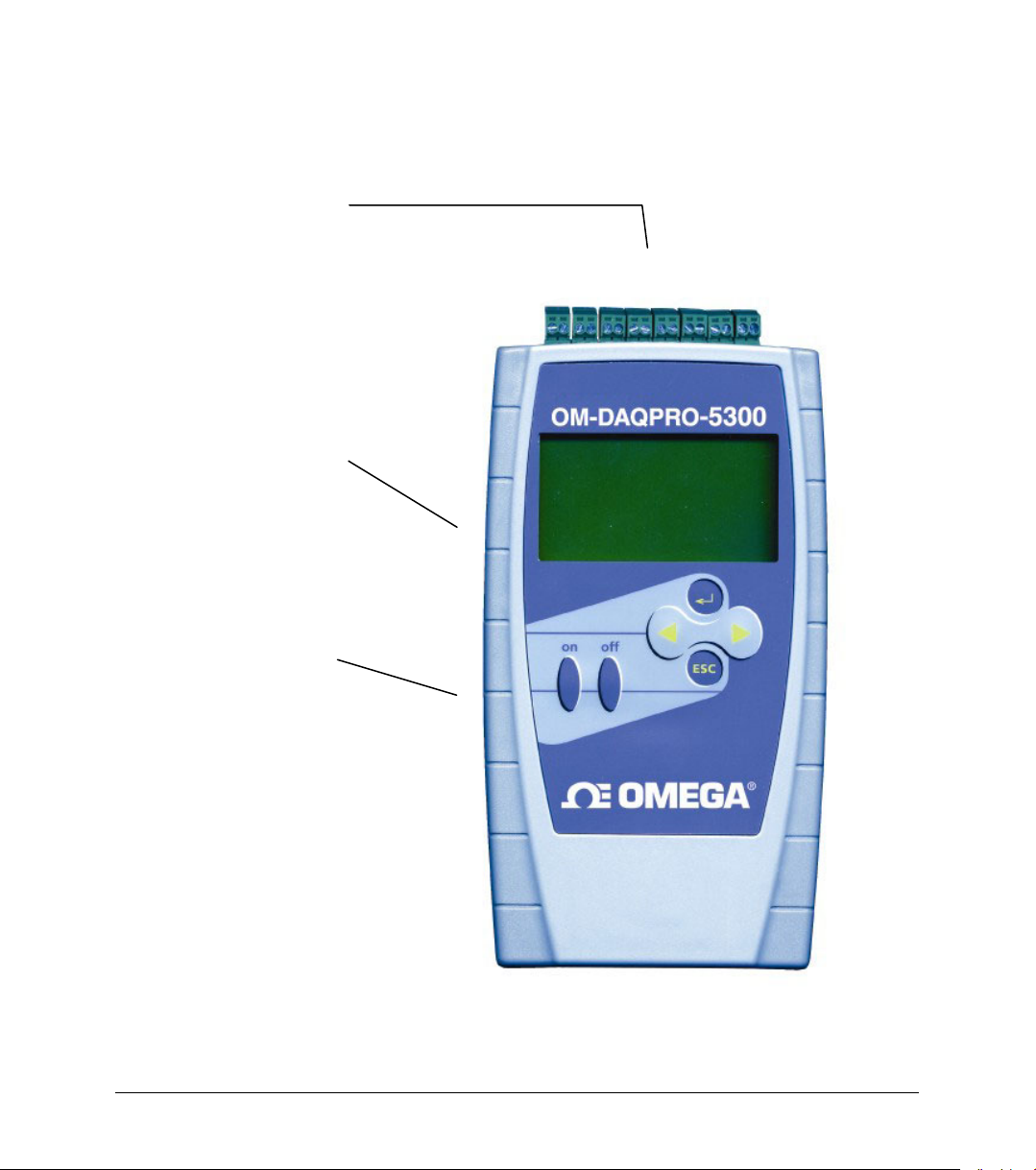
1.1.2. External connections

1. Sensor

Inputs/alarm
output

2. PC USB

connection
socket

8th

input/output

1st

ut

in

3. Power input

(DC 9 – 12V)

Figure 1: OM-DAQPRO-5300 external connections

10 Chapter 1 OM-DAQPRO-5300

1. Sensor inputs/alarm output – pluggable screw terminal block (marked Input -1 to Input – 8 from
right to left). All eight inputs can be used simultaneously.

If you are using one sensor, connect it to input 1. If you are using two sensors connect them to
inputs 1 and 2, and so on…

I/O–8 (Input/Output–8) serves either as an input or as alarm output.

To connect a sensor to the OM-DAQPRO-5300 unplug the screw terminal, connect the sensor’s
wires to the terminals, and then plug the terminal back to the corresponding socket on the input
block.

2. Computer USB communication socket – use this socket to connect OM-DAQPRO-5300 to a
computer

Connect the USB Type B plug (square plug) of the supplied communication cable to the OM­DAQPRO-5300 and the USB Type A plug (flat plug) to the computer (see page 32 for USB driver
installation).

3. External DC power supply socket – Plug in an AC/DC 9 - 12V adaptor whenever you want to
save battery power, or to charge the battery when necessary. Connecting external power to the
OM-DAQPRO-5300 automatically charges the internal battery. The adaptor should meet the
required specifications (see section 1.1.10 on page 15).

1.1.3. Sensor types and connections

Each of the 8 input channels of OM-DAQPRO-5300 is multipurpose and can be individually configured
to any of the following types and ranges:

Sensor Type Range

Current 0 – 24mA

Frequency (input 1 only) 20 to 4000Hz

Pulse counter (input 1 only) 0 to 65,000 pulses

Temperature Internal

Temperature

Temperature

Temperature PT-100 2 wire

Temperature PT-100 3 wire

Temperature Thermocouple J

Temperature Thermocouple K

Temperature Thermocouple T

Voltage 0 – 10V

Voltage 0 - 50mV

Chapter 1 OM-DAQPRO-5300 11

NTC 10KΩ -25 to 150°C

NTC 2252Ω -25 to 150°C

-25 to 70°C

-200 to 400°C

-200 to 400°C

-200 to 1200°C

-250 to 1200°C

-200 to 400°C

User defined Up to 20 types 0 – 10V or 0 – 24mA

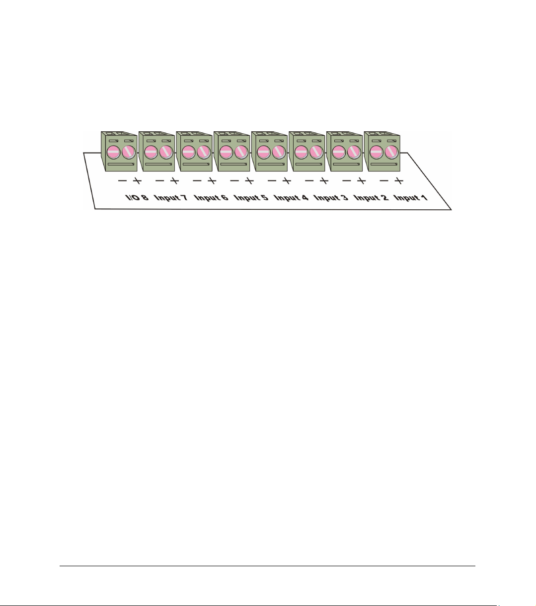
Connect the sensor to the terminal block at the top of OM-DAQPRO-5300:

Figure 2: OM-DAQPRO-5300’s inputs block terminal

Sensors must be added successively, starting with input–1. If a single sensor is used it must be
connected to Input–1. If two sensors are used, they must be connected to Input-1 and Input-2 and so
on…

Alarm output

I/O–8 (Input/Output–8) serves either as an input or as alarm output.

Polarity

Current, voltage, thermocouples and user defined sensors have distinct polarity. Be careful to connect
them in the right polarity.

Frequency/Pulse counter

Connect the signal wires to I/O–8 screw terminals, and select Frequency or Pulse counter for input 1
from the Setup menu. Inputs 2 to 7 are still available for other sensors.

The Frequency/pulse counter is optically isolated from the internal circuitry and can simultaneously
measure a signal source, together with another input.

3 wire PT 100

You have to use two inputs to connect a 3 wire PT 100 You can connect one 3 wire PT 100 to input–1
and input–5, and/or inputs 2 and 6, and/or inputs 3 and 7 and/or inputs 4 and 8.

Connect the single wire to the plus (+) terminal of the first input and the common end wires to the minus
(-) terminals of both the inputs. See Figure 3 for wiring configuration of a 3 wire PT 100 connected to
input–1 and input–5:

12 Chapter 1 OM-DAQPRO-5300

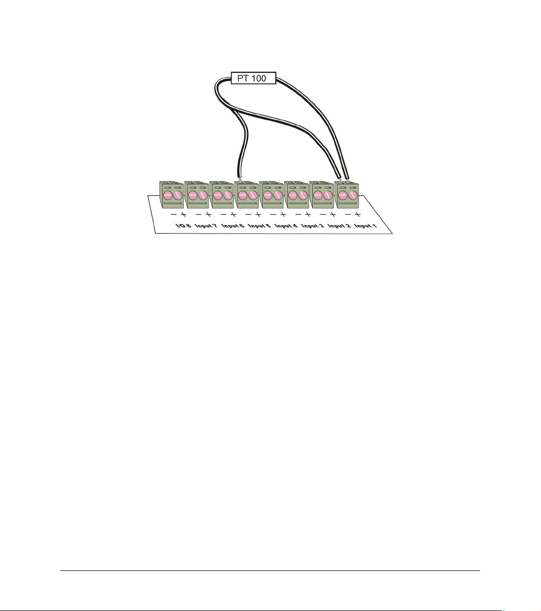
Figure 3: connecting 3 wire PT 100

When working with a 3 wire PT 100 inputs 5 to 8 are not available and you can connect up to 4 sensors.

Sensor mismatch

After logging begins OM-DAQPRO-5300 checks if the sensor type assigned to each channel matches
the attached sensor. If there is a mismatch, OM-DAQPRO-5300 disconnects the corresponding input
and displays a warning message: “Illegal sensor” (see ‘Troubleshooting Guide’ on page 86 for details)

1.1.4. User defined sensors

OM-DAQPRO-5300 provides a simple and straightforward tool for defining up to 20 custom sensors.
Almost any 0 – 10V and 0 – 24mA sensor or transducer is accepted by MultiLogPRO and its electrical
units are automatically scaled to meaningful user-defined engineering units.

The sensor definitions are stored in OM-DAQPRO-5300’s memory and are added to the sensors list.
The sensor’s readings are displayed in the user defined units both on OM-DAQPRO-5300’s LCD screen
and DaqLab software.

To learn how to define custom sensors see section 2.5.9 on page 68

For further manipulating sensors readings use the Analysis wizard (see page 73)

1.1.5. Alarms

Users can define minimum and maximum alarm levels for each input individually.

Chapter 1 OM-DAQPRO-5300 13

OM-DAQPRO-5300 places a small alarm icon next to the corresponding input readings and can
switch alarm output if either level is breached.

To display alarm warnings in real-time OM-DAQPRO-5300 must be in numeric display mode (see page

20).

To learn how to enter alarm levels and to activate alarm output, see section 2.5.1.2 on page 54.

1.1.6. Alarm output

OM-DAQPRO-5300 can trigger an external event (e.g. sound alarm, warning light or oven).

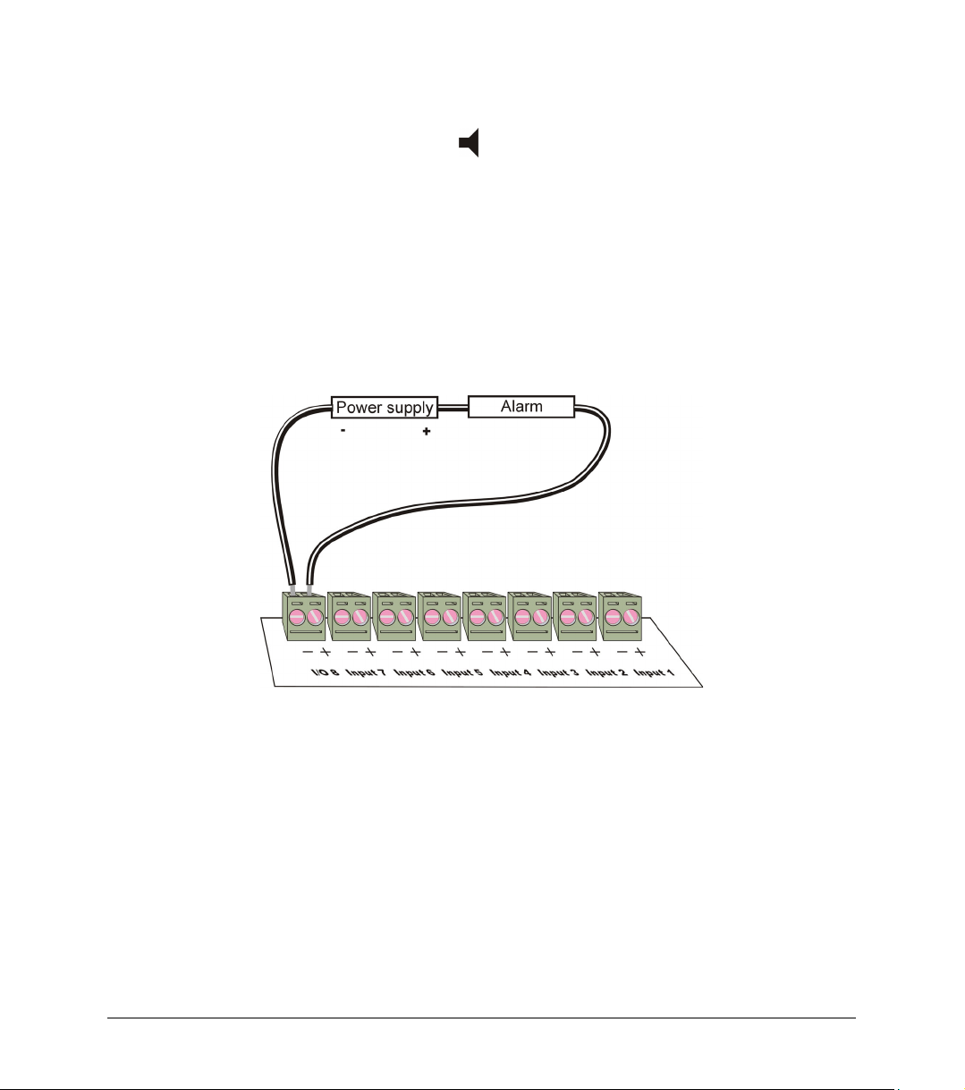
Connect the external current loop to the screw terminals of I/O–8. Be careful to connect the external
power supply in the right polarity (see Figure 4 below).

Figure 4: connecting external alarm device

The alarm output is analogous to electrical switch. In OFF position the terminals of I/O–8 are
disconnected. In ON position they are shortened.

If an alarm output is selected this input/output is set to OFF position. When any active alarm level is
exceeded the output is set to ON. All active alarms must be false to reset the output to OFF position.

The maximum switch load is 50mA, 5V. The output is protected by 50mA reset-able fuse. For higher
loads use a relay.

To learn how to enter alarm levels and to activate alarm output, see section 2.5.1.2 on page 54

14 Chapter 1 OM-DAQPRO-5300

1.1.7. Sensor calibration

OM-DAQPRO-5300 ships fully calibrated. However, further calibration can be applied via DaqLab. The
calibration parameters are sent to OM-DAQPRO-5300 and stored in its memory. See page 61 for
calibration instructions.

1.1.8. Serial number and comment

Every OM-DAQPRO-5300 unit is embedded with a unique serial number and can be loaded with a
descriptive comment to identify its task and location.

To add or edit the comment connect OM-DAQPRO-5300 to the computer and use DaqLab software (see
page 59).

Every time data is transferred to the computer it is labeled both with OM-DAQPRO-5300’s serial number
and comment and then displayed in the graph title.

The serial number is marked on the back of the product. To view its comment, select System information
from OM-DAQPRO-5300’s main menu.

1.1.9. Battery

OM-DAQPRO-5300 is equipped with a 7.2V Ni-MH rechargeable battery. Before you first start working
with OM-DAQPRO-5300, charge the unit for 10 to 12 hours while it is turned off. Battery life is
approximately 40 hours between charges.

If the data logger’s main battery runs out, the internal 3V Lithium battery backs up the memory, so no
data will be lost. The Lithium battery also keeps the internal clock and calendar running.

Note: Before storing the data logger make sure you have unplugged all the sensors and

pressed the OFF key.

1.1.10. Mains Adaptor

The Mains adaptor (AC/DC adaptor) converts mains power (from a wall outlet) to a voltage suitable to
OM-DAQPRO-5300.

• Output: Capacitor filtered 9 to 12 VDC, 400mA.

• Female plug, center Negative.

Chapter 1 OM-DAQPRO-5300 15

1.2. Stand-Alone Operation

One way to program the OM-DAQPRO-5300 is to use its keypad and screen (The other way is to use
the DaqLab software – see page 52). The keypad allows us to set all the parameters for data collection,
while the LCD screen displays the setting values.

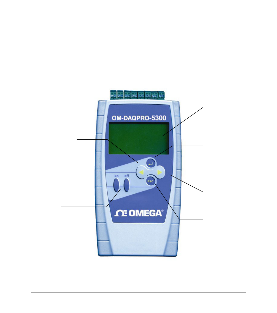
1.2.1. Front Panel Layout

LCD Display

Backward Button

Enter / Run Button

On / Off

Buttons

Figure 5: OM-DAQPRO-5300 front panel

16 Chapter 1 OM-DAQPRO-5300

Forward Button

Escape / Stop Button

1.2.2. Quick-Start

Before you first use OM-DAQPRO-5300, charge the unit for 10 to 12 hours while it is turned off.

1. Turn on OM-DAQPRO-5300

Press the on button. You will see the initialization screen. OM-DAQPRO-5300 performs a brief self­check and display its status including battery level and operating mode. At this point you can load the
last setup you used (see page 25). If you need a new setup wait until you see the Main Menu screen:

fn

?

2. Connect the sensors

Start with the first input on the right.

Note: Sensors must be added successively, starting with input 1. If a single sensor is

used it must be connected to Input 1. If two sensors are used, they must be
connected to Input 1 and Input 2.

See Sensors types and connections on page 11 for more details

3. Identify the Sensors

You must tell OM-DAQPRO-5300 what type of sensor is connected to each input

Chapter 1 OM-DAQPRO-5300 17

1. In the Main Menu screen, use the Forward arrow buttons to

select the setup menu icon

2. Press the Enter button

→ Input – 1 Voltage 0–10V
Input – 2 Empty
Input – 3 Empty
Input – 4 Empty

RATE = Every sec
SAMPLES = 500
DISPLAY = numeric

3. Use the Forward

select the sensor in input 1 and then press the Enter button.
The arrow indicator will move to the second input.

4. Repeat this procedure with all the sensors you plugged in.

5. After the fourth sensor has been selected, the screen will list the next
4 sensors:

→ Input – 5 Empty
Input – 6 Empty
Input – 7 Empty
Input – 8 Empty

RATE = Every sec
SAMPLES = 500
DISPLAY = numeric

to enter the setup menu:

and Backward arrow buttons to

.

18 Chapter 1 OM-DAQPRO-5300

You can press the Enter button in the last input if you want to go back to the first input.

6. When you’ve finished selecting the sensors press the Escape button.

The arrow indicator will point to the Rate command.

4. Select Rate

Use the Forward

Enter button

OM-DAQPRO-5300 automatically switches to the next step in the setup process and the arrow moves to
the “samples” row.

5.Select total number of samples

Use the Forward

press the Enter button.

and Backward arrow buttons to select the desired rate, then press the

.

Input – 1 Curent 0–24mA
Input – 2 NTC 10K
Input – 3
Input – 4

RATE = Every 10 sec
→ SAMPLES = 500
DISPLAY = numeric

and Backward arrow buttons to select the number of samples, then

Chapter 1 OM-DAQPRO-5300 19

Input – 1 Microphone
Input – 2 Light
Input – 3
Input – 4

RATE = Every sec
SAMPLES = 10,000
→ DISPLAY = numeric

6. Choose display

Use the Forward

the Enter button

Note: When you turn the OM-DAQPRO-5300 off it will save the setup for the next

session.

7. Start recording

Press the Forward arrow button

and Backward arrow buttons to select the type of display, then press

.

Input – 1 Microphone
Input – 2 Light
Input – 3
Input – 4

SAMPLES = 500
DISPLAY = graphic
→ START = ( > ).

to start recording.

20 Chapter 1 OM-DAQPRO-5300

Or press the Enter button if you want to go back to the first item (Rate).

You can stop recording at any time by pressing the Escape button .

1.2.3. Working with the OM-DAQPRO-5300 Menus

Turning OM-DAQPRO-5300 on and off

Note: Pressing OFF will not erase the sample memory. The data stored in the memory

1.Main menu display

When turned on, OM-DAQPRO-5300 opens with a system information window and then displays the
main menu:

On

Off

will be kept for up to 5 years.

Turn OM-DAQPRO-5300 on

Turn OM-DAQPRO-5300 off

fn

?

Chapter 1 OM-DAQPRO-5300 21

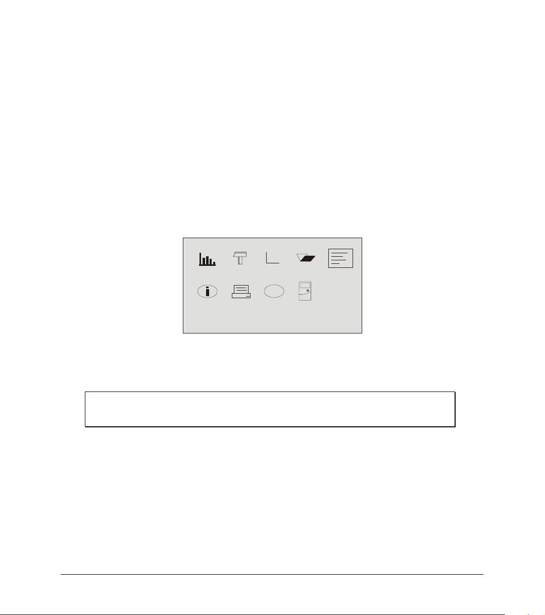
OM-DAQPRO-5300 has 9 menus. Use the Forward or Backward Arrow buttons to highlight a menu and
press the Enter button to select it. Then use the Arrow buttons to scan the options. Press the Enter
button to select an option. The OM-DAQPRO-5300 automatically executes the command.

2.Menu buttons

Forward

3.Menu Icons and commands

Backward

Enter (Start)

Escape (Stop)

Start

Press the Enter button to start recording

Setup

Rate – select recording rate

Move to the next menu or to the next menu options

Move to the previous menu or menu options

Enter the selected menu or select the current menu option and
move to the next menu command or start recording

Return to the main menu or stop recording

Start recording

Setup OM-DAQPRO-5300 in 4 steps:

22 Chapter 1 OM-DAQPRO-5300

Samples – select the total number of recording points

Display – select the way OM-DAQPRO-5300 will display the data (at a rate of

up to 1 sample per second):

1) Numeric – displays the sensor values and the sample number.

2) Meter – displays all active sensors in a bar meter display
along with their values (without decimals).

3) Table – displays the last 6 values of all the active sensors in
a table (without decimals).

4) Graphic – displays a graphic
representation of the
sampled sensors.

At rates higher then 1/s the OM-DAQPRO-5300 will display the data in a graph
at the end of the logging period.

Start – press the Forward arrow to start recording

fn

Function

1) Minimum – the minimum graph value.

2) Maximum – the maximum graph value.

3) Average – the graph average.

Use the Enter button to browse the different sensors

Open

Use the Forward and Backward Arrow buttons to browse the stored files,

press the Enter button to open a file

Notes

Use the Arrow buttons to browse the notes.

You can use the DaqLab software to edit the notes or to write new notes

Display statistics of the current data

Open a stored data in graphic display

Display user information

Chapter 1 OM-DAQPRO-5300 23

System
information

1) Comment (use DaqLab to enter a comment)

2) Number of files stored in OM-DAQPRO-5300’s internal memory

?

3) Memory usage

4) Battery level (unplug any sensor and external power supply)

5) Ambient temperature (the readings of the internal temperature sensor)

6) Current date and time

Help

Configuration

Filter – turn input filter on and off

Average – select number of averaging points

Temperature units – select between Fahrenheit and Celsius

Clear memory– delete the stored data files

Display system information:

On-line help and specifications

Configure the OM-DAQPRO-5300:

Contrast – use the arrow buttons to tune the screen contrast

1.2.4. Graphic Display

OM-DAQPRO-5300 will automatically use a graphic display in three cases:

1. If the recording rate is every second or less and you selected Graphic
Display in the setup menu

2. Once logging has ended for a recording rate of over one per second.

3. When opening a stored recording.

The graphic display is available for recordings with up to 4 sensors simultaneously.

24 Chapter 1 OM-DAQPRO-5300

2.The Cursor

Use the Cursor in Graphic Display mode to read data values or to zoom in to the area around a selected
point. The cursor is displayed automatically after logging has ended, or when opening a stored
recording.

1. Use the Forward
move the cursor.

2. OM-DAQPRO-5300 displays the point coordinates at the bottom of
the graph.

3. If there is more then one sensor, press the Enter button
move the cursor to another plot on the graph.

3. Zooming

1. Position the cursor in the area you want to zoom into.

2. Press the two arrow buttons,
will zoom in around the cursor in a 2:1 ratio.

3. Press the Escape button to zoom out.

and Backward arrow buttons to

to

and , simultaneously. You

1.2.5. Load the Last Setup

When you turn OM-DAQPRO-5300 on, once the self testing has been completed, it will display:

_ _ _ INITIALIZATION _ _ _

OM-DAQPRO-5300 Ver 1.0
Init. Display
Init. RAM
Batt. 99%

ENTER – load setup

Chapter 1 OM-DAQPRO-5300 25

Press the Enter button

to load the last setup.

1.2.6. Configure Your OM-DAQPRO-5300

Use the System configuration menu to turn input filter on and off, to select number of averaging points,
to set temperature units, to clear the OM-DAQPRO-5300’s memory or to change the screen contrast.

In the MAIN MENU screen, select the System configuration icon to display the configuration
screen:

_ _ _ CONFIGURATION _ _ _

→ Input filter Off
Average 4 samples
Temperature in ° C
Clear memory ( > )
Contrast ( < ) ( > )

Use the Forward

Enter button

configuration menu at any time, saving the new changes you made. Press Enter button in the last item
(Contrast) if you want to go back to the first item (Input Filter).

The new configuration will be saved until the next time you change it.

and Backward arrow buttons to select the mode and then press the

to move to the next item. You can press the Escape button to leave the

1. Input Filter

To filter out 50/60Hz line noises use the low pass RC input filter.

Use the Forward

When turned on, the low pass filter is applied to all inputs except for 24mA current measurements

26 Chapter 1 OM-DAQPRO-5300

and Backward arrow buttons to turn input filter on and off

2.Averaging points

Use this option to reduce random noises. OM-DAQPRO-5300 replaces every data sample with the
average of the last preset number of samples.

Use the Forward

3.Temperature units

Use the Arrow buttons to select between Fahrenheit (°F) and Celsius (°C) temperature units.

4.Clear memory

Press the Forward arrow button
DAQPRO-5300.

5.Screen contrast

Use the arrow buttons to adjust the LCD screen contrast.

Any contrast adjustment will be saved until the next time you change it.

and Backward arrow buttons to select the number averaging samples.

if you want to delete all previous data files from the OM-

1.2.7. Internal Clock and Calendar

The internal clock is set the first time you use the Setup command from the DaqLab software to program
the OM-DAQPRO-5300, and is automatically updated to the PC’s time and date each time you connect
your OM-DAQPRO-5300 to a PC.

The internal clock and calendar is kept updated independent of the 7.2V battery condition, even when
the OM-DAQPRO-5300 is turned off.

1.2.8. Clear the Memory

If you want to start recording and the OM-DAQPRO-5300’s internal memory is full you will see this
message at the bottom of the display:

Chapter 1 OM-DAQPRO-5300 27

Input – 1 Voltage 0–10V
Input – 2 Empty
Input – 3 Empty
Input – 4 Empty

SAMPLES = 200
DISPLAY = graphic
Mem full, clear = ( > )

Press the Forward arrow button

In order to clear the OM-DAQPRO-5300’s memory when it is not full, use the Memory clear command
from the Configuration menu (see page 26), or clear the memory from the Logger menu in the
DaqLab software (see page 59).

to clear the memory

1.2.9. Choose the Right Setup.

1. Sampling rate - The sampling rate should be determined by the rate of change of the
phenomenon being sampled. If the phenomenon is periodic, sample at a rate of at least twice the
expected frequency. Changes in temperature can be measured at slower rates such as once per
second or even slower, depending on the speed of the expected changes. Usually it’s a good
practice to sample at a rate 10 times higher than the expected frequency but for extremely smooth
graphs, the sampling rate should be about 20 times the expected frequency.

Note: Sampling at a rate slower than the expected rate can cause "frequency aliasing".

In such a case, the graph will show a frequency much lower than expected. In
Figure 6 below, the higher frequency sine wave was sampled at 1/3 of its
frequency. Connecting the sampled points yielded a graph with a lower, incorrect
frequency.

28 Chapter 1 OM-DAQPRO-5300

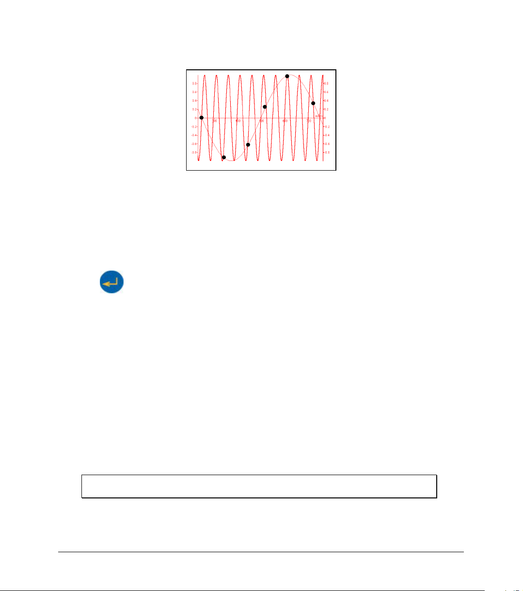
Figure 6: Frequency Aliasing

Manual sampling - use this mode for:

• Recordings or measurements that are not related to time.

• Situations in which you have to stop recording data after each sample

obtained, in order to change your location, or any other logging parameter
(Note: During recording NO CHANGES can be made to the OM-DAQPRO­5300’s configuration).

To start a recording using manual data logging, set the RATE to “manual” and press the Enter

button
collect a sample.

2. Sampling Points - After you have chosen the sampling rate, choosing the number of points will
determine the logging period: Samples / Rate = Logging time. You can also choose the duration of
a run first, and then calculate the number of samples: Samples = Logging time × Rate.

Continuous

In the Continuous mode, OM-DAQPRO-5300 must be connected to the PC and the DaqLab software
must be running. In this mode OM-DAQPRO-5300 can continue logging indefinitely. The data is
automatically downloaded to the computer, displayed in a real time graph and saved every 10 minutes.

OM-DAQPRO-5300 stores the data until its memory is full. You can download this data only if you
stopped logging before this point

To operate in Continuous mode select RATE equal to or less than 1/s and SAMPLES = Continuous.

You can also select Continuous mode directly from the DaqLab software.

Note: OM-DAQPRO-5300 must be set to a display mode other than graphic to enable

Chapter 1 OM-DAQPRO-5300 29

once to start the data recording, then press the Enter button each time you want to

the Continuous mode.

1.2.10. Programming Rules and Limitations

The following are some rules and limitations you must take into account when programming the OM­DAQPRO-5300, as OM-DAQPRO-5300 integrates all programming limitations automatically. OM­DAQPRO-5300 will only allow the programming of settings that comply with the rules below.

1.Sampling rate:

The number of sensors in use limits the maximum sampling rate:

1. Maximum sampling rate with one sensor is 4000/s

2. Maximum Temperature sampling rate is 1/s

3. Maximum sampling rate with two sensors or more is 1/s

4. Maximum sampling rate with two or more PT 100 sensors or more is every 10
seconds

5. Maximum sampling rate with eight PT 100 sensors or more is every minute

6. OM-DAQPRO-5300 displays readings in real time at rates up to 1/s

7. DaqLab displays online readings at rates up to 100/s

2.Sampling points:

Increasing the number of active inputs limits the number of sampling points one can choose. The
following condition must be always satisfied:

Number of samples × Active Inputs ≤ Memory

OM-DAQPRO-5300’s memory is sufficient for 512,000 samples.

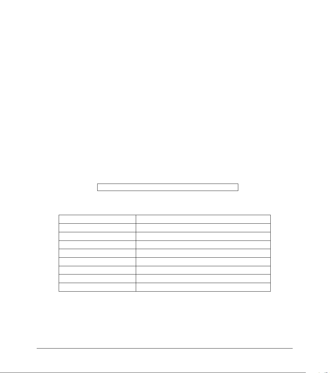
The table below lists the maximum number of sampling point according to the number of sensors:

Number of sensors Maximum number of sampling points

1 512,000 (exact number: 522,752)

2 256,000 (exact number: 260,608)

3 128,000 (exact number: 129,536)

4 128,000 (exact number: 129,536)

5 64,000

6 64,000

7 64,000

8 64,000

3.Continuous sampling

• Continuous sampling is possible up to a maximum sampling rate of 1/s.

• The data must be presented in a display mode other than graphic.

30 Chapter 1 OM-DAQPRO-5300

Chapter 2

Working with DaqLab

2.1. Install the Software

2.1.1. System Requirements

To work with DaqLab, your system should be equipped with the following:

1.Software

 Windows 98 or later

 Internet Explorer 5.0 or later (you can install Internet Explorer 5 when you install

DaqLab, since it ships with the product)

2.Hardware

 Pentium 200MHz or higher

 32 MB RAM (64 MB recommended)

 10 MB available disk space for the DaqLab application (50 MB to install the supporting

applications)

2.1.2. Installation

1. Close all programs

2. Insert the CD labeled DaqLab into your CD-ROM drive

Installation will begin automatically. Simply follow the on-screen instructions to continue

In case auto run is not working, open My Computer and click on the CD drive folder (d: drive in most
cases) and double-click on the setup icon, then follow the on-screen instructions.

To uninstall the software: From the Start menu select Settings and click on Control Panel, then use
the Add/Remove programs function to remove the DaqLab application.

When updating the software, always remove the old version before starting a new installation.

Chapter 2 Working with DaqLab 31

To install the USB driver:

1. Insert the CD into your CD drive. If Installation begins automatically
(and you have already installed DaqLab), click Cancel to stop
installation

2. Connect the OM-DAQPRO-5300 to a USB port on your PC and turn
the OM-DAQPRO-5300 on. Windows will automatically detect the new
device and open the Add New Hardware Wizard

3. Select Specify the location of the driver, then click Next

4. Select Search for the best driver for your device, then check the
Removable Media checkbox, and then click Next

Windows will automatically detect and install the necessary software.

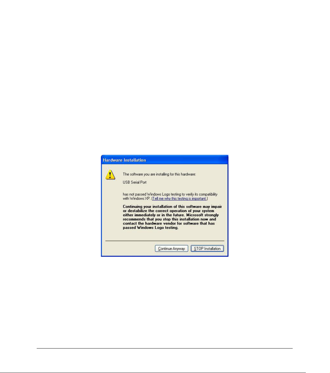
Note to the Windows XP user – if the found New Hardware wizard prompts you to a Hardware
Installation dialog:

Just click Continue Anyway to proceed.

32 Chapter 2 Working with DaqLab

2.2. Overview

2.2.1. DaqLab On-screen Layout

DaqLab is a comprehensive program that provides you with everything you need in order to collect data
from the OM-DAQPRO-5300 display the data in graphs, meters and tables and analyze it with
sophisticated analysis tools.

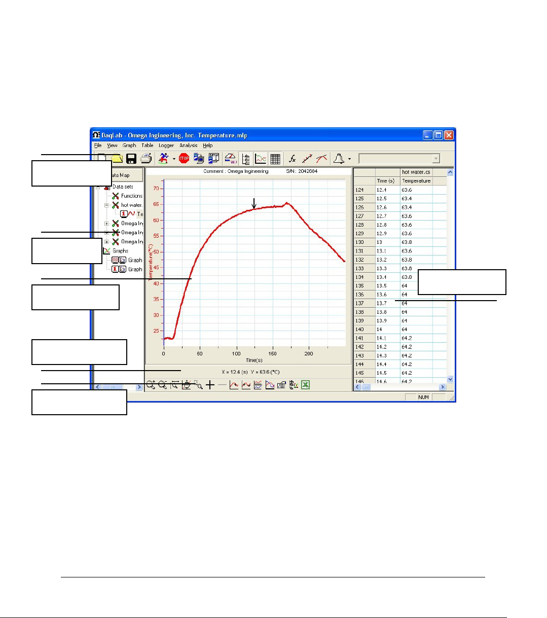
The program includes three windows: A graph window, table window, and a navigation window called the
Data Map. You can display all three windows simultaneously or in any combination.

The most commonly used tools and commands are displayed on two toolbars. Tools that relate to all
aspects of the program and tools that control the OM-DAQPRO-5300 are located in the main (upper)
toolbar. Tools specific to the graphs are located on the graph (lower) toolbar.

2.2.2. Working with Projects

Every time you start a new recording, DaqLab automatically creates a new project file. All the information
you collect and process for a given session is stored in a single project file. Each of these files contain all
the data sets you collect with the OM-DAQPRO-5300, the analysis functions you’ve processed, specific
graphs you’ve created, and the DaqLab settings for the recording.

Note: all data sets in a single project must be with the same sampling rate.

Chapter 2 Working with DaqLab 33

2.2.3. DaqLab Window Layout

Main toolbar

Data map

Graph window

Table window

Information bar

Graph toolbar

34 Chapter 2 Working with DaqLab

Figure 7: DaqLab window layout

2.3. Getting Started

2.3.1. Set up a Recording Session

1. Prepare OM-DAQPRO-5300

1. Connect OM-DAQPRO-5300 to the PC (see page 10)

2. Turn on OM-DAQPRO-5300

3. Plug in any external sensors

4. Open the DaqLab software

You can open DaqLab by double clicking its icon

2. Setup the OM-DAQPRO-5300

1. Click Setup Wizard

2. Follow the instructions in the Setup Wizard (see page 52)

3. Start Recording

Click Run

If the recording rate is 100 measurements per second or less, DaqLab automatically opens a graph
window displaying the data in real time, plotting it on the graph as it is being recorded. If the recording
rate is higher than 100/s, the data will be downloaded and displayed automatically, once the data
recording is finished.

You can stop recording anytime by clicking Stop

on the toolbar to start recording.

on the main toolbar

on the desktop or from the start menu

on the toolbar.

Chapter 2 Working with DaqLab 35

2.3.2. Data recording options

To set the behavior of the data display when you start a new recording session, click on the down arrow

next to the Run button

1.Single measurement

DaqLab will open a new project file every time you start a new recording session.

2. Replace

DaqLab will display the new data set in place of the old set. The project’s old data sets will still be
available in the same project file. They will be listed in the Data Map and you can add them to the
display at any time

3. Add

DaqLab will add the new data set to the graph in addition to the old ones.

Note: A maximum of 8 data sets can be displayed on the graph at the same time.

, and select one of the following:

2.3.3. Download Data

Whenever data is received from the OM-DAQPRO-5300, it is accumulated and displayed automatically
by DaqLab. There are two modes of communication: online and offline.

Online communication

When OM-DAQPRO-5300 is connected to the PC and programmed to run at sampling rates of up to
100/s, OM-DAQPRO-5300 transmits each data sample immediately, as it is recorded, to the PC. The
software thus displays the data in real-time in both the graph window and the table window.

When OM-DAQPRO-5300 is connected to the PC and programmed to run at a sampling rate of 500/s or
higher, data is accumulated in OM-DAQPRO-5300‘s internal memory. This data is not transmitted to the
PC until the recording period has ended, when the data is automatically downloaded to the PC and
displayed.

Offline data logging

• To download data that was recorded offline, or while OM-DAQPRO-5300 was not

connected to a PC, connect OM-DAQPRO-5300 to the computer, run the DaqLab

36 Chapter 2 Working with DaqLab

program and click Download on the main toolbar. This will initiate the Post­Recording Data Transfer communication mode. Once the transfer is complete, the
data will be displayed automatically in the graph window and in the table window. If
there are several files stored in the OM-DAQPRO-5300, the first download will bring
up the most recent file; the second download will bring up the second most recent file,
and so on.

• If you are logging offline at rates of up to 1/s, you can connect OM-DAQPRO-5300 to

the computer and download the accumulated data at anytime. Apart from during the
transfer period, the data will be downloaded without interrupting the logging process.

• To download a particular file, choose Selective download from the Logger menu,

then select the file’s number in the Download dialog.

• Click Cancel in the Download progress window at any time to stop downloading the

data.

2.3.4. Save Data

Click Save on the main toolbar to save your project. This will save all the data sets and graphs
under one project file.

Saving the project will also save any special formatting and scaling you did.

If you made any changes to a previously saved project, click Save to update the saved file or select

Save as… from the file menu to save it under another name.

Note:

To delete a specific data set, a graph or a table from the project, use the Data Map (see
page 49)

To remove unwanted data from a specific data set, apply the crop tool (see page 82).

2.3.5. Open a File

1. Click Open on the main toolbar

2. Navigate to the folder where the project is stored

Chapter 2 Working with DaqLab 37

3. Double click the file name to open the project

DaqLab opens the project and displays the first graph on the graph list. If the project does not include
saved graphs, the file opens with an empty graph window. Use the Data Map (see page 49) to display
the desired data set.

2.3.6. Create a New Project

There are three ways to create a new project:

1. Open the DaqLab program, which will open a new file each time

2. When working in Single Measurement mode, a new project is opened
every time you click on the Run button to start a new recording

3. Any time you click New button

on the toolbar

2.3.7. Import data

Any file that is in comma separated values text format (CSV) can be imported into DaqLab

To import a CSV file:

1. Click File on the menu bar, then click Import CSV file

2. In the dialog that opens, next to Look in, navigate to the drive and
folder that contains the CSV file

3. Select the file

4. Click Open

Tips:

To create a text file in a spreadsheet:

1. Open a new spreadsheet

2. Enter your data according to the following rules:

a) The first row should contain headers. Each header includes the name

of the data set and units in brackets, e.g. Distance (m)

38 Chapter 2 Working with DaqLab

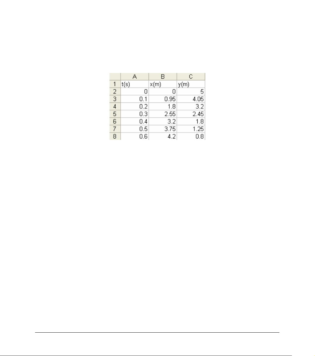
b) The first column should be the time. The time interval between

successive rows must match the time intervals accepted by DaqLab.
You can export DaqLab files to Excel to learn about these time formats

See for example the table below:

3. On the File menu, click Save As

4. In the File name box, type a name for the workbook

5. In the Save as type list, click the CSV format

6. Click Save

To import files that were previously exported from DaqLab open DaqLab and import the file as described
above as they are already in CSV format.

2.3.8. Date format settings

To set the way data will be displayed on screen click Date format settings to open the Date format
settings dialog:

Chapter 2 Working with DaqLab 39

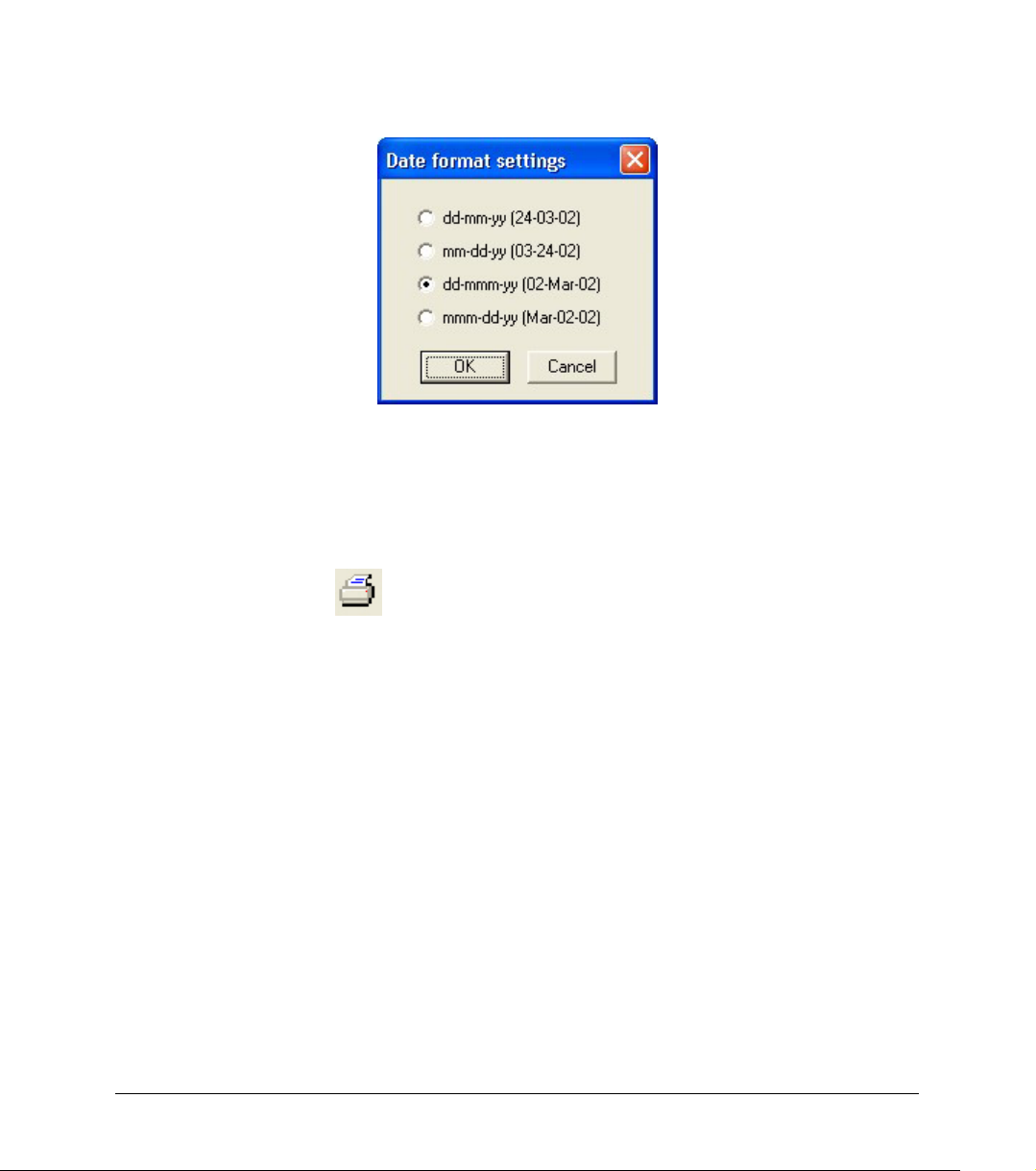
Click the desired option, then click OK

2.3.9. Print

1. Print a graph

1. Click Print

2. Select the Graph 1 option (when in split graph mode you can choose
between Graph 1 and Graph 2)

3. Click Print to open the print dialog

4. Click OK

DaqLab will print exactly what you see in the graph display.

40 Chapter 2 Working with DaqLab

on the main toolbar

2. Print a table

1. Click Print

2. Select the Table option

3. If you want to print only a specific range, uncheck the Print all data
check box and type the desired row numbers into the To and From
edit boxes

4. Click Print to open the print dialog

5. Click OK

DaqLab will print exactly what you see in the table display as well as the OM-DAQPRO-5300 comment,
serial number and the alarm level setup. Data that exceeds any of the alarm levels will be highlighted by
arrows.

on the main toolbar

Chapter 2 Working with DaqLab 41

2.4. View the Data

2.4.1. Display Options

The DaqLab program’s screen consists of three parts: the graph window, table window and Data Map
window. You can display all three parts simultaneously (the default view) or any combination of the
three.

The graph window is the main window by default and is and displayed in the center of the application
window.

In addition to these sections, you have the option to display an on-screen meter for each of the sensors
(see page 48).

2.4.2. Graph Display

Click Graph to display or hide the graph. The default graph display is the data set or sets plotted
vs. time, but you can change the X-axis to represent any of the individual data sets (see page 44).

The graph usually displays all the data sets of a given recording, but you can use the Data Map to
remove one or more of the sets from the graph (see page 49).

In order to keep the graph clear and simple, only two Y-axes are shown on the graph at once. If there
are three curves in the graph, one of the Y-axes is hidden. In order to make this axis visible, select the
corresponding plot with the cursor (see section 2 below).

You can identify the Y-axis by its color, which matches the plot color.

1. Split graph view

DaqLab enables you to display your data in two separate graphs within the graph window.

1. Click Split graph
into two separate graphs

2. Click Edit graph
dialog

3. Choose which data sets to display on each of the graphs (or use the
Data Map to do so – see page 49)

42 Chapter 2 Working with DaqLab

on the graph toolbar to split the graph window

on the graph toolbar to open the Edit graph

4. To return to the single graph display, click Split graph a second
time

2. The Cursor

You can display up to two cursors on the graph simultaneously.

Use the first cursor to display individual data recording values, to select a curve or to reveal the hidden
Y-axis.

Use two cursors to display the difference between two coordinate values, to display the frequency of
periodic data or to select a range of data points.

To display the first cursor:

Double click on an individual data point or click Cursor

on the graph toolbar. You can drag the
cursor with the mouse onto any other point on the plot, or onto a different plot. For finer cursor
movements use the forward and backward keys on the keyboard.

The coordinate values of the selected point will appear in the information bar at the bottom of the graph
window.

To display the second cursor:

Double click again anywhere on the graph area or click 2

nd

Cursor .

The information bar will now display the difference between the two coordinate values.

To remove the cursors:

Double click anywhere on the graph area, or click 1

st

Cursor a second time.

To remove the 2nd cursor:

Click 2nd Cursor a second time.

To display the cursors in split graph mode:

To display the cursors on the upper graph, use the same method as for single graph mode.

To display the cursors on the lower graph, you must first remove them from the upper graph and then
double click anywhere on the lower graph to display the first cursor. Double click a second time to
display the second cursor, and double click a third time to remove the cursors.

3. Zooming

1. To zoom in to the center of the graph

1. Click Zoom in

on the graph toolbar

Chapter 2 Working with DaqLab 43

2. To reverse the operation, click Zoom out on the graph toolbar

2. To zoom in to a specific data point

1. Select the point with the cursor (see above)

2. Click Zoom in

3. To reverse the operation click Zoom out on the graph toolbar.

3. To zoom in to a range

1. Select the range with both cursors

2. Click Zoom in on the graph toolbar

3. To reverse the operation click Zoom out on the graph toolbar

4. To zoom in to a specific area

Click Zoom to selection
want to magnify. Release the mouse button to zoom in to the selected area.

Click Zoom to selection a second time to disable the zoom tool.

5. Autoscale

Click Auto scale
auto scale that axis alone.

6. Manual scaling

on the graph toolbar to view the full data display, or double click on an axis to

on the graph toolbar

on the graph toolbar and drag the cursor diagonally to select the area you

1. Click Graph properties
properties dialog

2. Select the Scale tab, and choose the axis you want to scale in the
Select axis drop list

44 Chapter 2 Working with DaqLab

on the graph toolbar to open the Graph

3. Uncheck the Autoscale check box and enter the new values in the edit
box

4. Click OK

To manually scale a specific axis, right click on the axis to open its Properties dialog.

To restore auto scaling click Autoscale

7. The stretch/compress axis tool

Move the cursor onto one of the graph axes. The cursor icon changes to the double arrow symbol (
indicating that you can stretch or compress the axis scale. Drag the cursor to the desired location.

Repeat the procedure for the other axis if necessary.

Double click on the axis to restore auto scaling.

4. Panning

Use the pan tool after zooming in to see any part of the graph that is outside the zoomed area.

To do this, click Pan
view another area.

Click Pan a second time to disable the Pan tool.

5. Edit the Graph

Use the Edit graph dialog to select which data sets to display on the graph’s Y-axis and to change the
X-axis from time, to one of the data sets.

1. Click Edit graph
dialog:

on the graph toolbar, then click anywhere on the graph and drag the mouse to

.

↔),

on the graph toolbar to open the Edit graph

Chapter 2 Working with DaqLab 45

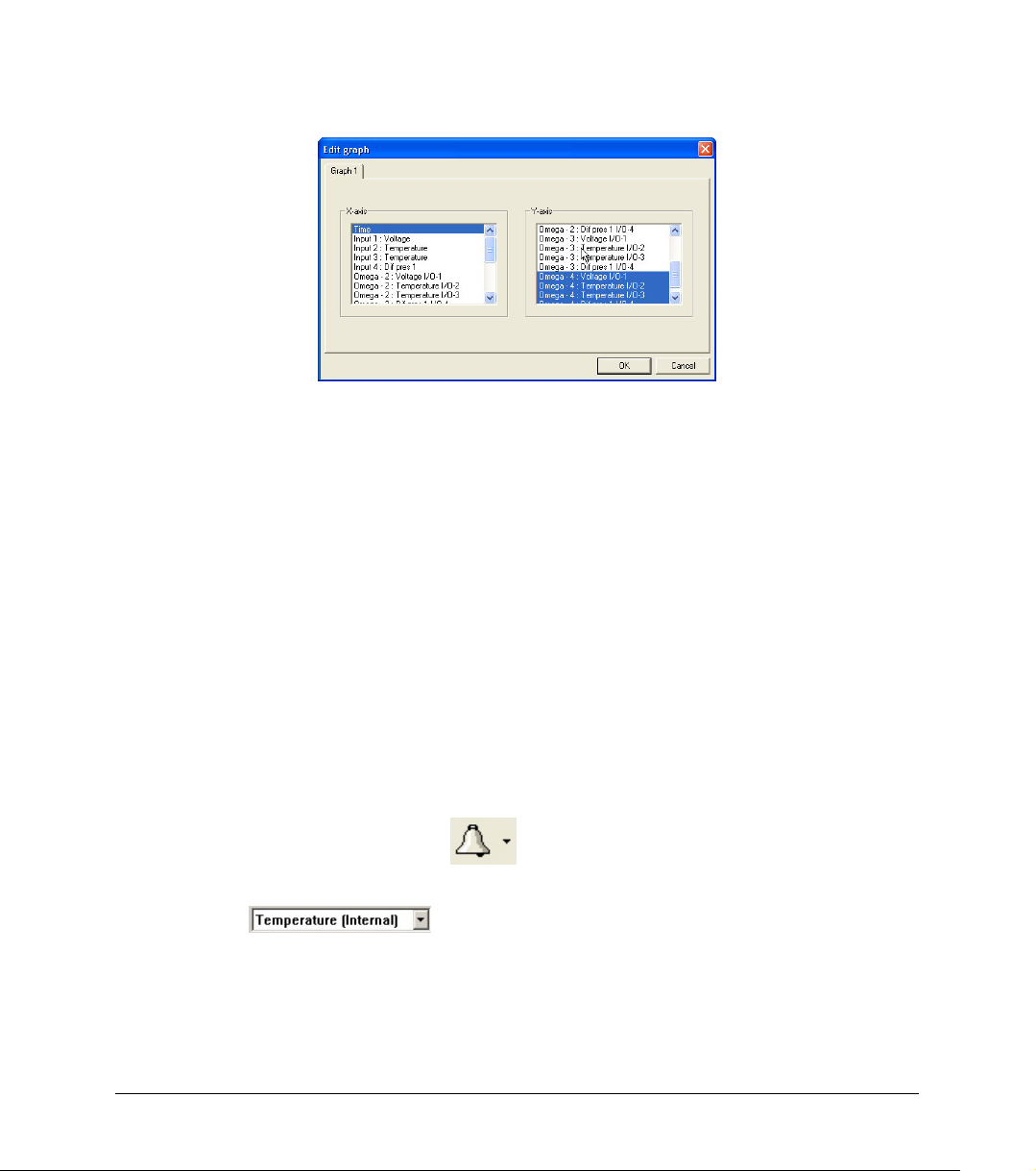
Figure 8: Edit graph dialog

2. To select a data set to display on the Y-axis, click on the data set’s
name in the Y-axis list. To display more than one curve, click on the
data sets you want

3. A list entry that begins with a OM-DAQPRO-5300 comment denotes a
recorded data set. A list entry that begins with an input number
denotes the next recording and will be displayed on the graph the next
time you start a recording

4. To deselect a data set, click on it a second time

5. To select a data set for display on the X-axis, click on the data set’s
name in the X-axis list. You can only select one data set at a time for
the X-axis

6. Click OK

6. Display alarm levels

1. Click Display alarm level

2. Select the sensor you wish to display from the select sensor drop list

To display alarm levels on graph 2 in split graph mode click the down arrow next to the button and select
graph 2.

7. Format the graph

46 Chapter 2 Working with DaqLab

.

You can change the data line’s color, style and width. You can also add markers that represent the data
points on the graph and format their style and color.

The color of the Y-axis matches the corresponding plot’s color and will automatically change with any
change made to the color of the corresponding plot.

1. Click Graph properties
properties dialog

2. Select the Lines tab, and then select the plot or axis you want to
format in the Select plot drop list

3. From here you can format the line’s color, style and width, as well as
the markers’ color and style. To remove the line or the marker,
uncheck the corresponding Visible check box

4. Click OK

5. To restore the default formatting, click Restore default

8. Change the graph’s units and its number format

1. Click Graph properties
properties dialog

2. Select the Units tab, and then select the plot or axis you want to
format in the select plot drop list

3. Choose the prefix option you want

4. Select the desired number of decimal places

5. To display numbers in scientific format, check the Scientific check
box

on the graph toolbar to open the Graph

on the graph toolbar to open the graph

6. Click OK

9. Add a graph to the project

DaqLab displays new data in the graph window every time you start a new recording. You can always
display previous data using the Edit graph dialog or by double-clicking on the data’s icon in the Data

Chapter 2 Working with DaqLab 47

Map. If you want to save a graph that you created to your project, or to update a saved graph with
changes you made, use the Add to project tool:

Click Add to project on the graph toolbar.

2.4.3. The Table Display

Click Table to display or to remove the table window.

The data in the table always matches the data that is currently displayed on the graph.

When you start a new recording, DaqLab displays the new data in the table as well as on the graph.

48 Chapter 2 Working with DaqLab

Formatting the table

1. Changing column width

Drag the boundary on the right side of the column heading until the column is the desired width.

2. Changing row height

Drag the boundary below the row heading until the row is the desired height.

3. Formatting the fonts

1. Click Table on the menu bar, then click Properties

2. Select the Font tab

3. Format the font, as well as the font’s style and size

4. Click OK

4. Changing units and number format

1. Click Table on the menu bar, then click Properties

2. Select the Units tab, and then select the plot you want to format from
the select plot drop list

3. Choose the prefix option you want

4. Select the desired number of decimal places

5. To display numbers in scientific format, check the Scientific check
box

6. Click OK

2.4.4. Meters

DaqLab enables you to view data in meters format on the screen (one meter for each sensor), with up to
four meters showing at once. The meters can display live data while DaqLab is recording, or saved data
when a saved file is replayed.

When a cursor is displayed, the meter shows the measured values that correspond to the time of the
point at which the cursor is positioned.

There are three meter types: analog, bar and digital. The meter’s scaling automatically matches the
graph’s scaling.

Chapter 2 Working with DaqLab 49

To set up the meters:

1. Click Meter Setup

2. Select the meter type, and the data set to be displayed

3. A list entry that begins with a graph number denotes a displayed data
set. A list entry that begins with an input number denotes the next
recording, and will be displayed on the meter the next time you start a
recording

4. Repeat this procedure for up to four meters

5. To remove the meters click Meter Setup

on the main toolbar

, and click Remove all

2.4.5. Data Map

Click Data Map to display or remove the Data Map.

The data map is a separate window that displays the list of data sets that were recorded or downloaded
in the current session, as well as the lists of all the saved graphs. Use the Data Map to navigate through
the available data sets and to keep track of the data that is being displayed in the graph window.

Note: The data in the table always matches the data that is currently displayed on the

graph.

1. Control the display with the Data Map

The items in the Data Map are sorted into two main categories:

• Data sets (including analysis functions)

• Saved graphs

Double click on a category to bring up the full list. Double click a second time to collapse the list. You
can also use the plus (+) and minus (-) signs next to the icons to expand or collapse the categories.

The Data sets' list expands to sub-categories of recorded data and functions. To display the complete
list of measurements, or the complete list of analysis functions performed on the measurements for any
individual data capture, double click the file’s icon or click the plus sign (+) next to it.

To collapse a list under an individual data capture, double click the corresponding icon or click the minus
sign (-) next to it.

50 Chapter 2 Working with DaqLab

To display a data set or a saved graph double click its icon. Double click a second time to remove it.

You can also use a shortcut menu to display or remove a data set from the graph. Simply right-click an
icon, then click display on graph #1 or display on graph #2.

To delete an individual item from the Data Map and from the project, right-click on its icon and click

Delete. To permanently delete the item, click Save

To remove all data sets from the Data Map, right-click the Data sets icon

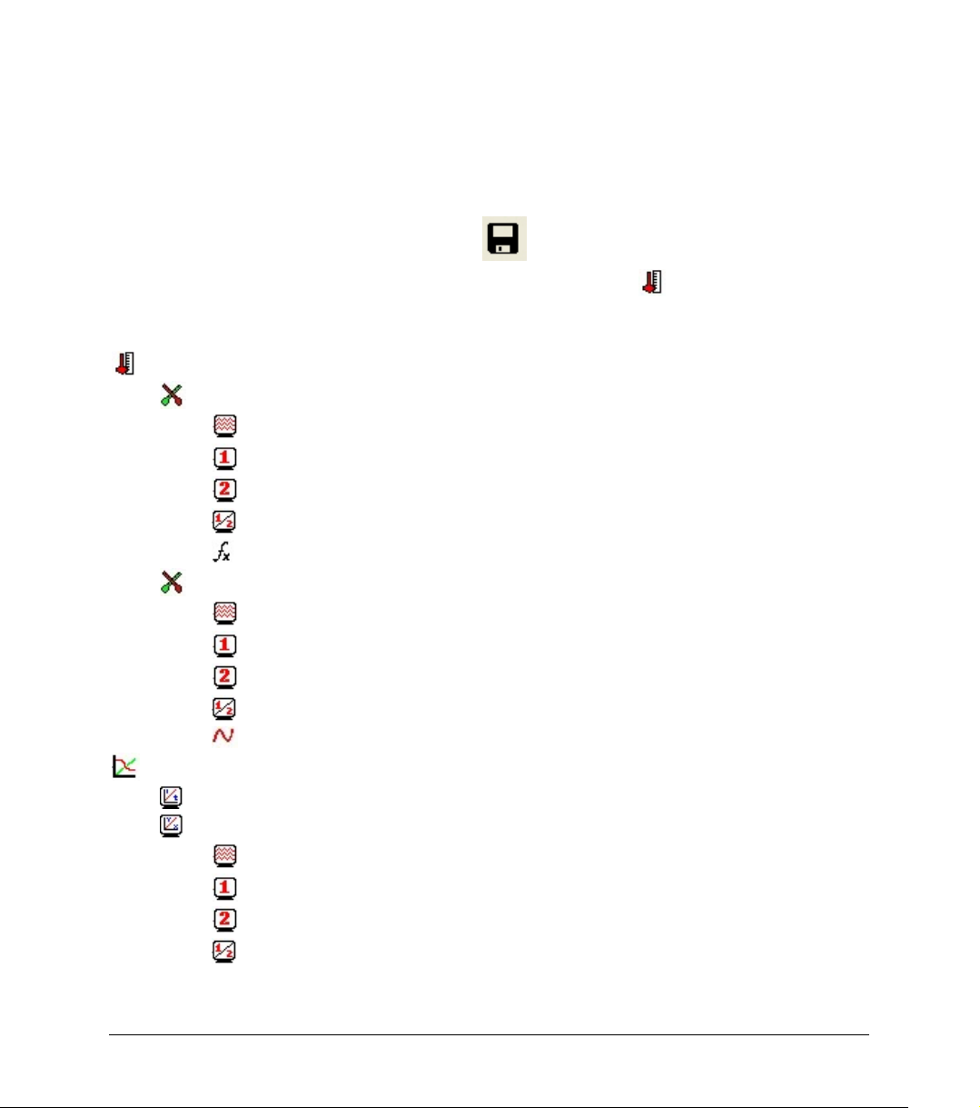
2. Understanding Data Map icons

Data sets list

Functions – includes all the analysis functions of the project

Individual function – currently not on display

Individual function – currently displayed on graph 1

Individual function – currently displayed on graph 2

Individual function – currently displayed both on graphs 1 and 2

Function

data capture – includes all recorded data of the recording

Individual data set – currently not on display

Individual data set – currently displayed on graph 1

Individual data set – currently displayed on graph 2

Individual data set – currently displayed both on graphs 1 and 2

Raw data

List of saved graphs

Saved graph – data sets vs. time

Saved graph – data sets vs. data set

Graph currently not on display

Graph currently displayed on graph 1

Graph currently displayed on graph 2

Graph currently displayed both on graphs 1 and 2

on the main toolbar.

and click Clear All Data.

Chapter 2 Working with DaqLab 51

2.4.6. Export Data to Excel

Click Export to Excel on the graph toolbar to export the data that is currently displayed on the
graph to Excel. DaqLab will then open a new Excel workbook displaying the data as well as the OM­DAQPRO-5300 comment, serial number and the alarm level setup. Data that exceeds any of the alarm
levels will be highlighted by arrows.

Export file settings

If DaqLab fails to export the data properly, try to change the export file settings:

1. Click File on the menu bar, then click Export file settings

2. Check the Ignore regional settings check box

3. Click OK

2.4.7. Copy the Graph as a Picture

You can copy the graph to the clipboard as a picture and then paste it to other Windows programs such
as Word or PowerPoint:

1. In the Graph menu, click Copy graph

2. Open the destination file

3. In the destination file, right click and select Paste

52 Chapter 2 Working with DaqLab

2.5. Program OM-DAQPRO-5300

2.5.1. Setup

1. Quick setup

Use the Setup wizard to guide you through the setup process.

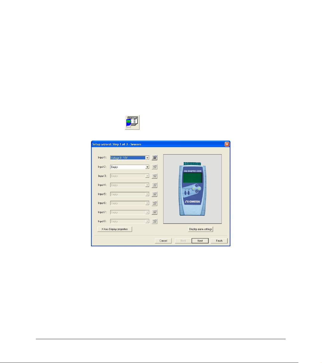
1. Click Setup wizard on the main toolbar to open the setup
wizard:

Figure 9: Setup wizard step 1 of 3

The first step is to assign sensors to each input. Select the sensors
you are using from the corresponding input drop lists.

To set alarm levels and alarm action click Display alarm settings
(see page 54 for detailed alarm setup)

2. Click Next to move to the second step:

Chapter 2 Working with DaqLab 53

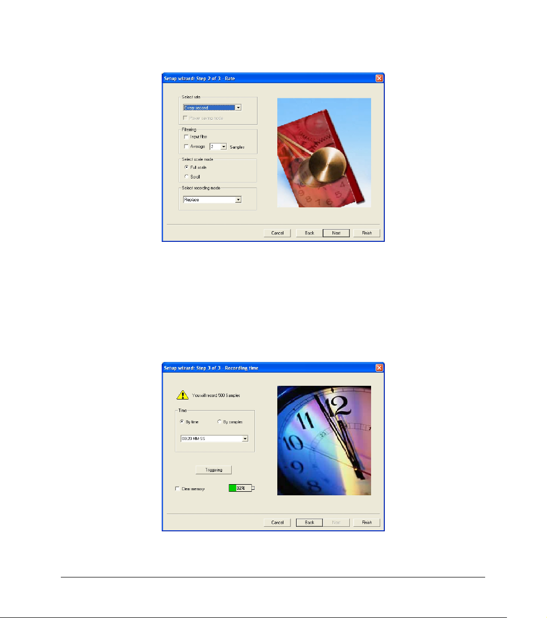
Figure 10: Setup wizard step 2 of 3

3. Select the desired recording rate in the Select rate drop list

4. Select the Scroll option if you want the graph window to scroll as the
data recording progresses

5. Select the desired data recording mode in the Select recording
mode drop list

6. Click Next to move to the third step:

54 Chapter 2 Working with DaqLab

×

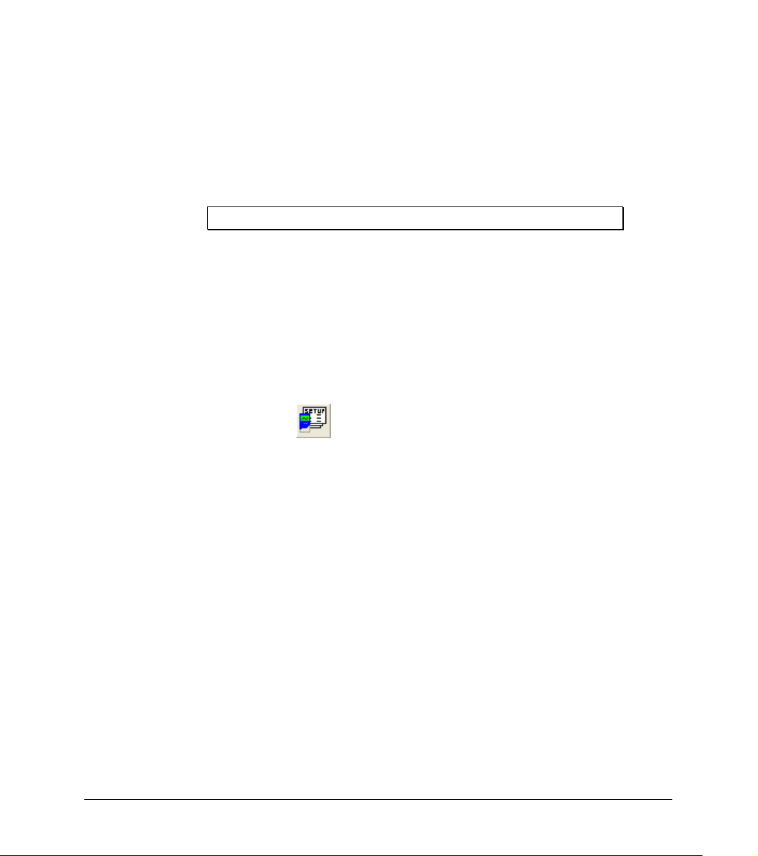
Figure 11: Setup wizard step 3 of 3

7. Select the desired length of the recording period in the Select
recording time drop list. The recording period is displayed as a unit
of time by default. To display the recording period as the number of
recording samples, select the By samples option. The number of
samples is calculated with the following formula:

Total recording samples

8. To start the data recording only when a specific time or measurement
condition has been met click Triggering to open the triggering dialog
(see page 57)

9. Click Finish to complete the setup and to send the setup command to
the OM-DAQPRO-5300

2. Alarm setup

You can setup alarm levels and output for each sensor input individually in the first step of the Setup
wizard:

1. Click Setup Wizard
wizard

2. Click Display alarm settings to show the alarm controls:

on the main toolbar to open the setup

=

Recording periodRecording rate

Chapter 2 Working with DaqLab 55

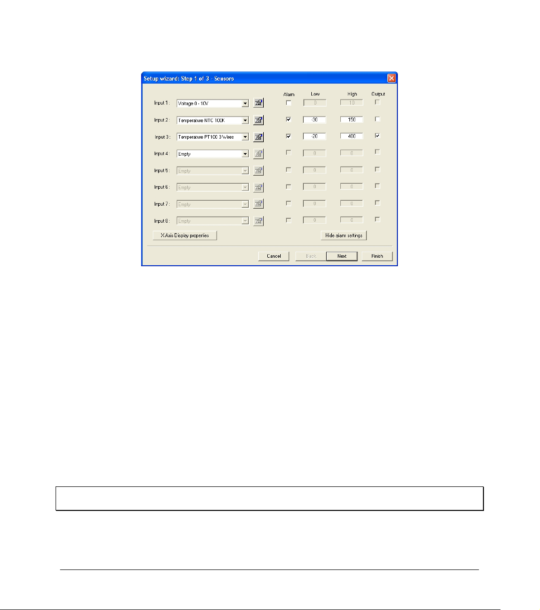
Figure 12: alarm settings

3. Check the checkbox or checkboxes near the inputs you want to
activate the alarm

4. Type in Low or/and High alarm levels

5. If you want a sensor or sensors to activate the alarm output check the
corresponding Output checkbox or checkboxes

6. Click Next to proceed to step 2 of the setup wizard or click Finish to
complete the alarm setup

See page 13 to learn more on alarms and alarm output.

You can set DaqLab to display the alarm levels on the graph window (see page 45)

3. Low pass filter

To filter out 50/60Hz line noises use the low pass RC input filter:

Check the Input filter checkbox in step 2 of the Setup wizard

Note: We strongly recommend to use the filter with low output sensors like 50mV voltage measurements

and thermocouples.

The low pass filter is applied to all inputs except for 24mA current measurements

56 Chapter 2 Working with DaqLab

4. Averaging

Use this option to reduce random noises. OM-DAQPRO-5300 replaces every data sample with the
average of the last pre-set number of samples

To apply averaging:

Check the Averaging checkbox in step 2 of the Setup wizard, and select the number of samples to
average from the drop list

5. Battery level

A battery level indicator is displayed in step 3 of the Setup wizard. The indicator shows the remaining
working hours as a percent of the battery’s life (approximately 40 hours between charges), before it
should be recharged.

6. Presetting the display

You may want to define the graph’s settings, such as formatting and scaling the graph and selecting the
axes, and to define the meters’ settings prior to beginning a recording session. You can define the
settings of each sensor input individually in the first step of the Setup wizard:

1. Click Setup Wizard
wizard

2. Click Properties

3. Click the Display properties tab

4. Select a measurement from the Select measurement drop list

5. Select the graph or graphs in which you would like to display the data,
from the Display on graph drop list

6. Select a meter in the Meter type drop list if you want to display the
data in a meter as well as on the graph

7. Format the line and markers in the Plot section

8. If you want a specific scale, uncheck the Auto scale check box and
enter the desired minimum and maximum values of the axis

9. Click OK

Chapter 2 Working with DaqLab 57

on the main toolbar to open the setup

next to the input you want to set

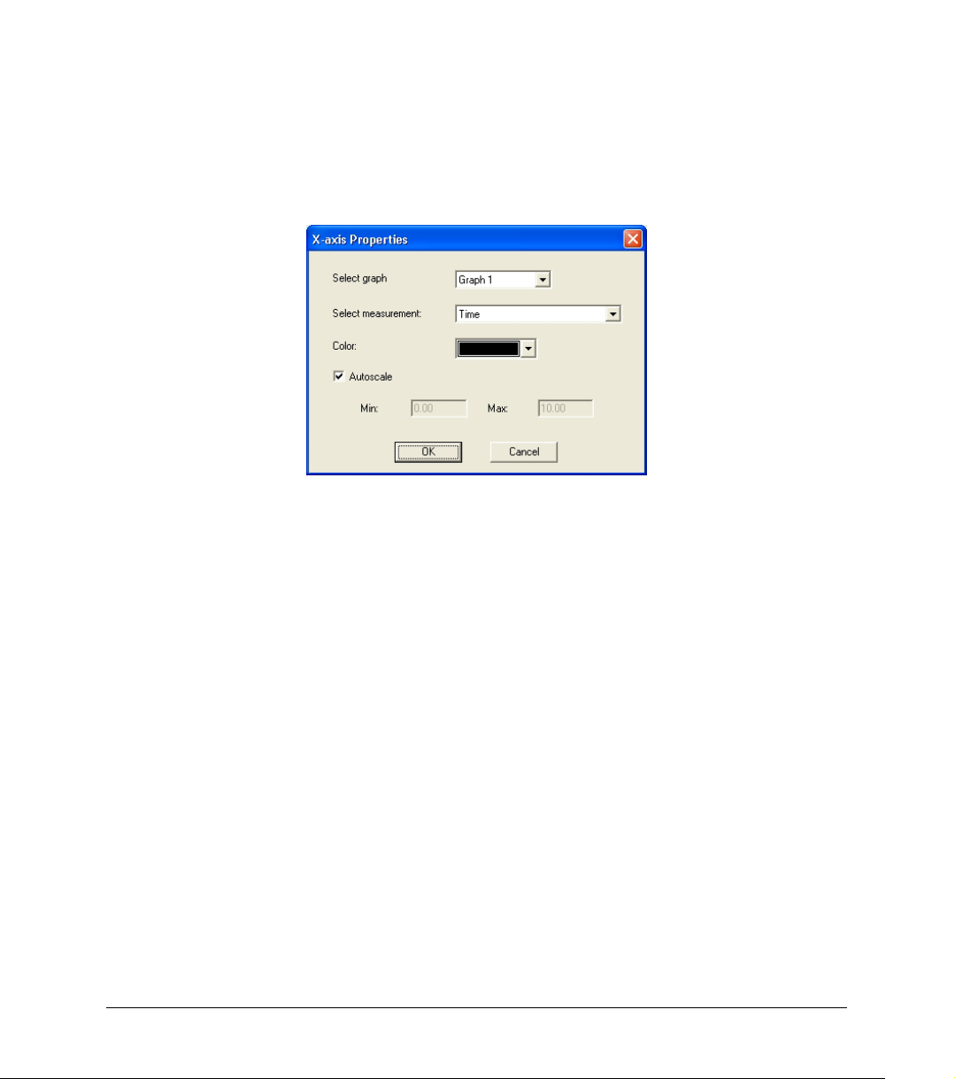
7. Preset the graph’s X-axis

1. Click X-Axis display properties in the first step of the Setup wizard
to open the dialog:

Figure 13: X-axis properties dialog

2. Select the graph you wish to modify

3. Select the measurement you’d like to display on the X-axis

4. If you want a specific scale, uncheck the Auto scale check box and
enter the minimum and maximum values of the axis

5. Click OK

8.Triggering

To start the data recording only when a specific time or measurement condition has been met, click
Triggering in step 3 of the Setup wizard to open the triggering dialog:

58 Chapter 2 Working with DaqLab

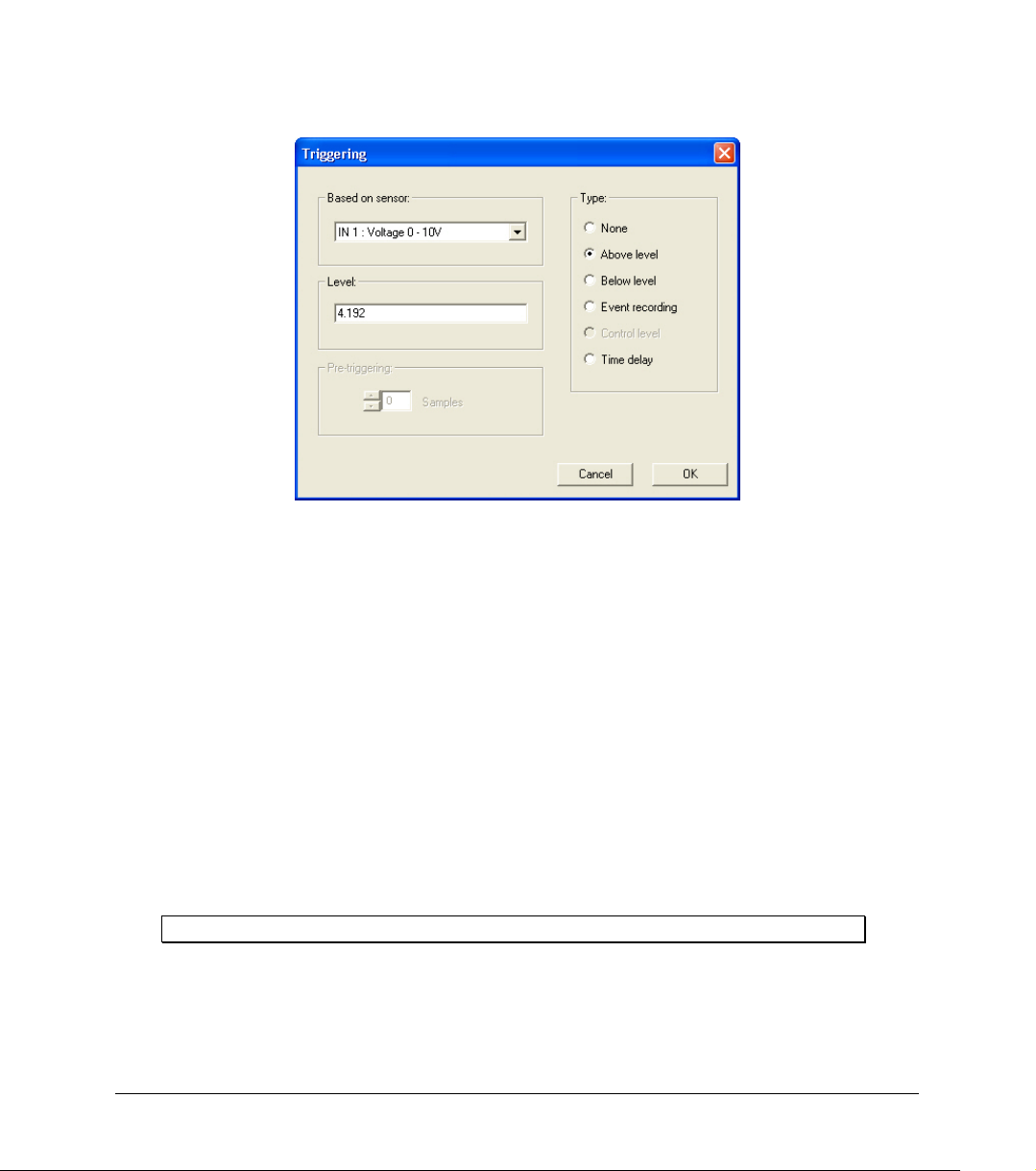
Figure 14: Triggering dialog

1. Select the triggering sensor in the Based on sensor drop list

2. Choose one of the following from the Type options:

• None – Trigger is disabled

• Above level – Start logging only once the measured value is

the trigger level.

• Below level – Start logging only once the measured value is

trigger level.

• Event Recording – This function enables you to record the exact time and

date at which a certain phenomenon occurred: The trigger level set for this
option is actually a threshold setting. Each time the threshold is crossed, OM­DAQPRO-5300 will record the exact time and date of the occurrence, and will
continue to do so until the desired number of samples has been obtained.

When logging has ended download the data to the PC (if OM-DAQPRO-5300 is already connected to
the PC it will be done automatically). The event list will be displayed in the table window. You can now
save the list, export it to Excel or print it.

HIGHER than

LOWER than the

Note: The trigger condition must be fulfilled for at least 300µS.

• Time delay – This trigger type enables you to set a timer that will start the

logging after a predetermined amount of time. After setting the trigger to Timer
Delay, click the down arrow on the Level combo-box, and select from the 17

Chapter 2 Working with DaqLab 59

different time options. The timer will start its countdown when you click RUN,
and the actual recording will start once the countdown has ended.

3. Select the trigger level in the Level edit box

4. Click OK

Note: When you turn off OM-DAQPRO-5300, it will save the setup for the next session.

2.5.2. Start Recording

Click Run on the main toolbar. Click the down arrow to change the recording mode.

2.5.3. Stop Recording

Click Stop on the main toolbar

2.5.4. Clear OM-DAQPRO-5300’s Memory

To erase all data currently stored in the OM-DAQPRO-5300, click Clear memory in the Logger menu
(OM-DAQPRO-5300 must first be connected to the PC).

2.5.5. Adding comment to OM-DAQPRO-5300

You can add a comment to each OM-DAQPRO-5300. The comment will serve as a name to identify the
specific OM-DAQPRO-5300 in addition to its serial number. Every time data is being downloaded from a
OM-DAQPRO-5300, its comment and the serial number will be displayed in the graph title and on the
corresponding icon in the Data Map. To display the comment on OM-DAQPRO-5300’s LCD select the
System information menu (see page 22)

The comment and the serial number will also be displayed in prints and exported files.

Note: the comment can include up to 32 characters.

To add a comment:

1. Connect OM-DAQPRO-5300 to the PC

2. Click Logger on the menu bar, then click Set comment

60 Chapter 2 Working with DaqLab

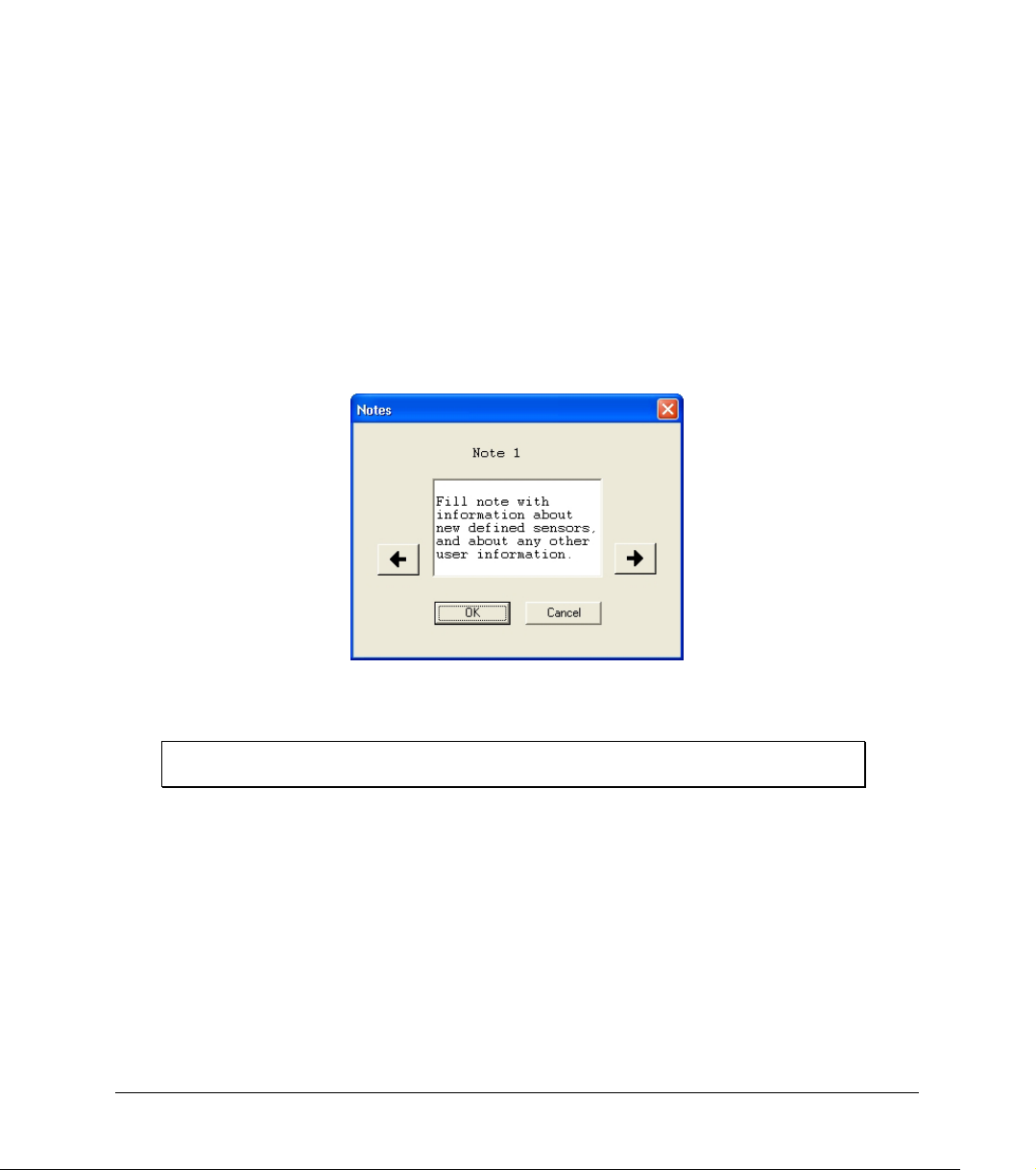
3. Click the Comment edit box and type a comment (e.g. its location)

4. Click OK to upload the edited notes to OM-DAQPRO-5300

2.5.6. Edit OM-DAQPRO-5300’s Notes

1. Connect OM-DAQPRO-5300 to the PC

2. Select Edit notes from the Logger menu to open the Notes dialog
with the OM-DAQPRO-5300’s current notes downloaded to the
window

Figure 15: Edit notes dialog

3. From this dialog, you can edit, delete, or write new notes

Note: A note is limited to 140 characters and a maximum of 3 notes can be stored in

OM-DAQPRO-5300 at any time.

4. Use the arrow buttons to move to the next note, or to the previous one

5. Click OK to upload the edited notes to OM-DAQPRO-5300

2.5.7. Temperature units

To select between Fahrenheit (°F) and Celsius (°C) temperature units:

Click Logger on the menu bar, point to Temperature units and then select the desired units

Chapter 2 Working with DaqLab 61

2.5.8. Calibrating the sensors

1.Calibration options

OM-DAQPRO-5300 ships fully calibrated. However, DaqLab enables you to calibrate any of the OM­DAQPRO-5300 sensors except for the internal temperature sensor, which doesn’t need calibration. The
calibration parameters are sent to OM-DAQPRO-5300 and stored in its memory.

Tips:

• Prior to any calibration procedure you must restore factory defaults

• Calibrating a sensor type applies to all inputs

• Calibrating the PT 100 2 wires sensor applies also to PT 100 3 wires except for fine

offset calibration

• Prior to calibrating any of the thermocouple sensor types, calibrate the Voltage 50mV

sensor as this will set the gain (slope) of all thermocouple sensor types

• The internal temperature sensor needs no calibration

DaqLab employs three different calibration methods Two-point calibration, Offset calibration and
Zero calibration. When selecting a sensor type to calibrate, DaqLab prompts you to the appropriate
calibration procedure:

Sensor Type Calibration method

Current 0 – 24mA Two-point calibration

Temperature

Temperature

Temperature PT-100 2 wire Two-point calibration

Temperature PT-100 3 wire Two-point calibration*

Temperature Thermocouple J Offset calibration

Temperature Thermocouple K Offset calibration

Temperature Thermocouple T Offset calibration

Voltage 0 – 10V Two-point calibration

Voltage 0 - 50mV Two-point calibration

NTC 10KΩ

NTC 2252Ω

Zero calibration

Zero calibration

Two-point calibration

The two-point calibration sets the gain (slope) and offset (intercept) of the sensor's conversion function.

62 Chapter 2 Working with DaqLab

Use the two point calibration to calibrate the voltage and current sensors and the PT100 temperature
sensors.

* To calibrate the PT100 3 wire, first calibrate the PT100 2 wire as the slopes of their conversion

functions are identical. Then proceed to adjust the PT100 3 wire offset.

In some cases you may need to refine your calibration using the fine offset tuning tool.

Offset calibration

To calibrate the thermocouple temperature sensors: TC-J, TC-K and TC-T first calibrate the 50mV
sensor type. That will set the slope for all thermocouple temperature sensors. Then proceed to adjust
the offset using the Offset calibration technique.

Zero calibration

The zero calibration sets only the offset (intercept) of the sensor's conversion function.

Use the zero calibration to calibrate the NTC 10kΩ and NTC 2252Ω temperature sensors.

2.Calibration password

To prevent accidental change of the calibration, the calibration procedure is protected by a password.

The default password is: 1234

To change the password:

1. Click Logger on the menu toolbar, and then click Calibration

2. Click Change Password to open the Change Password dialog box

3. Enter the current password in the Current Password edit box

4. Enter the new password in the New Password edit box

5. Enter the new password a second time in the Confirm New
Password edit box to confirm your new password

6. Click OK

Note: The password must include at least 4 characters and is case sensitive.

3.Calibration procedure

Two point calibration:

Measure two reference values

Chapter 2 Working with DaqLab 63

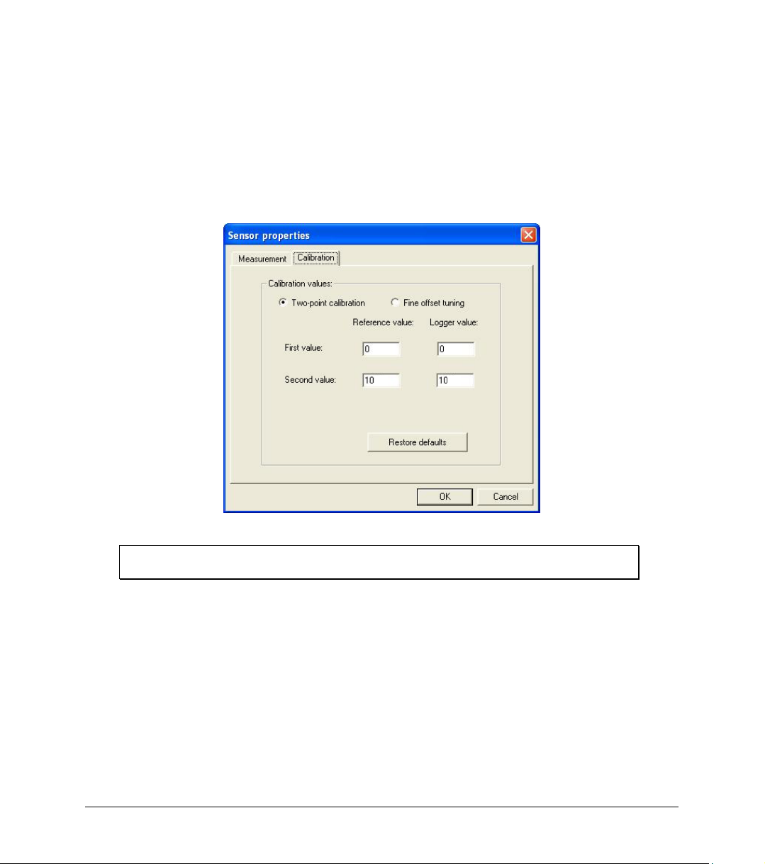
1. Connect OM-DAQPRO-5300 to the PC

2. Click Logger on the menu bar, then click Calibrate sensors

3. Enter the calibration password, then click OK

4. Choose a sensor from the Select sensor drop list and click OK to
open the Sensor calibration dialog:

Figure 16: Two-point calibration dialog

Note: we strongly recommend calibrating using the values that appear in the two

Reference value edit boxes

5. Click Restore defaults, then click OK

6. Measure two known reference values and record both the reference
values and the values displayed by DaqLab

64 Chapter 2 Working with DaqLab

Enter calibration values

 Repeat steps 1 to 4 above

7. Select the Two-point calibration option

8. Enter a distinct reference value in each of the Reference Value edit
boxes and the corresponding logger values in each of the Logger
Value edit boxes (The logger values are the values displayed by
DaqLab when measuring the two reference values)

9. Click OK

Fine offset calibration

If, after the calibration procedure, OM-DAQPRO-5300 still exhibits some offset value use the Fine offset
tuning tool to correct it.

The offset value is the difference between the value displayed by OM-DAQPRO-5300 and the reference
value. For example if the calibrator is set to 0°C and OM-DAQPRO-5300 reads 1°C the offset value is
+1, but if OM-DAQPRO-5300 reads −1°C then the offset value is −1.

1. Connect OM-DAQPRO-5300 to the PC

2. Click Logger on the menu bar, then click Calibrate sensors

3. Enter the calibration password, then click OK

4. Choose a sensor from the Select sensor drop list and click OK to
open the Sensor calibration dialog

5. Select the Fine offset calibration option

6. Enter the offset value

7. Click OK

The calibrated sensor parameters will be saved both in OM-DAQPRO-5300 and DaqLab memories, so
there is no need to calibrate OM-DAQPRO-5300 every time you run the DaqLab program.

Offset calibration:

Calibrating any of the thermocouple sensors comprises of two steps. First calibrate the 50mV voltage
sensor to set the slope of the sensor's conversion function. Then use the calibration procedure
described below to calibrate the sensor's offset.

Chapter 2 Working with DaqLab 65

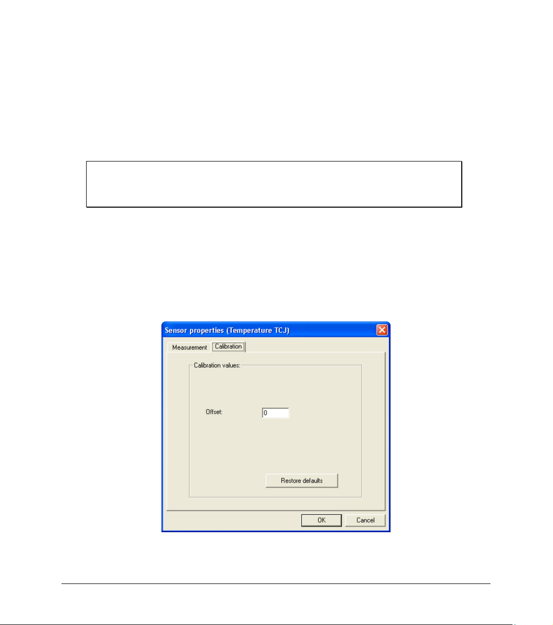
Measure two reference values

Before taking measurements you need to disable the temperature compensation both in OM­DAQPRO-5300 and in the calibrator.

To disable the temperature compensation in OM-DAQPRO-5300:

Click Logger on the menu bar, point to Thermocouple compensation, and then click Disable.

Note: don’t forget to enable the temperature compensation prior to normal operation of

OM-DAQPRO-5300. One way to enable the temperature compensation is to turn
OM-DAQPRO-5300 off and on again. Another way is via DaqLab: Click Logger
on the menu bar, point to Thermocouple compensation, then click Enable

To take two reference measurements:

1. Connect OM-DAQPRO-5300 to the PC

2. Click Logger on the menu bar, then click Calibrate sensors

3. Enter the calibration password, then click OK

4. Choose a sensor from the Select sensor drop list and click OK to
open the Sensor calibration dialog:

Figure 17: Offset calibration dialog

66 Chapter 2 Working with DaqLab

5. Click Restore defaults, then click OK

6. Measure two known reference values and record both the reference
values and the values displayed by DaqLab. Calculate the offset
values

The offset value is the difference between the value displayed by
OM-DAQPRO-5300 and the reference value. For example if the
calibrator is set to 0°C and OM-DAQPRO-5300 reads 1°C the offset
value is +1, but if OM-DAQPRO-5300 reads −1°C then the offset
value is −1.

Enter calibration values

1. Repeat steps 1 to 4 above

2. Enter the offset value in the Offset edit box (in case the two offset
values are not identical enter the average of the two values)

3. Click OK

Zero calibration:

1. Connect OM-DAQPRO-5300 to the PC

2. Click Logger on the menu bar, then click Calibrate sensors

3. Enter the calibration password, then click OK

4. Choose a sensor from the Select sensor drop list and click OK to
open the Sensor calibration dialog:

Chapter 2 Working with DaqLab 67

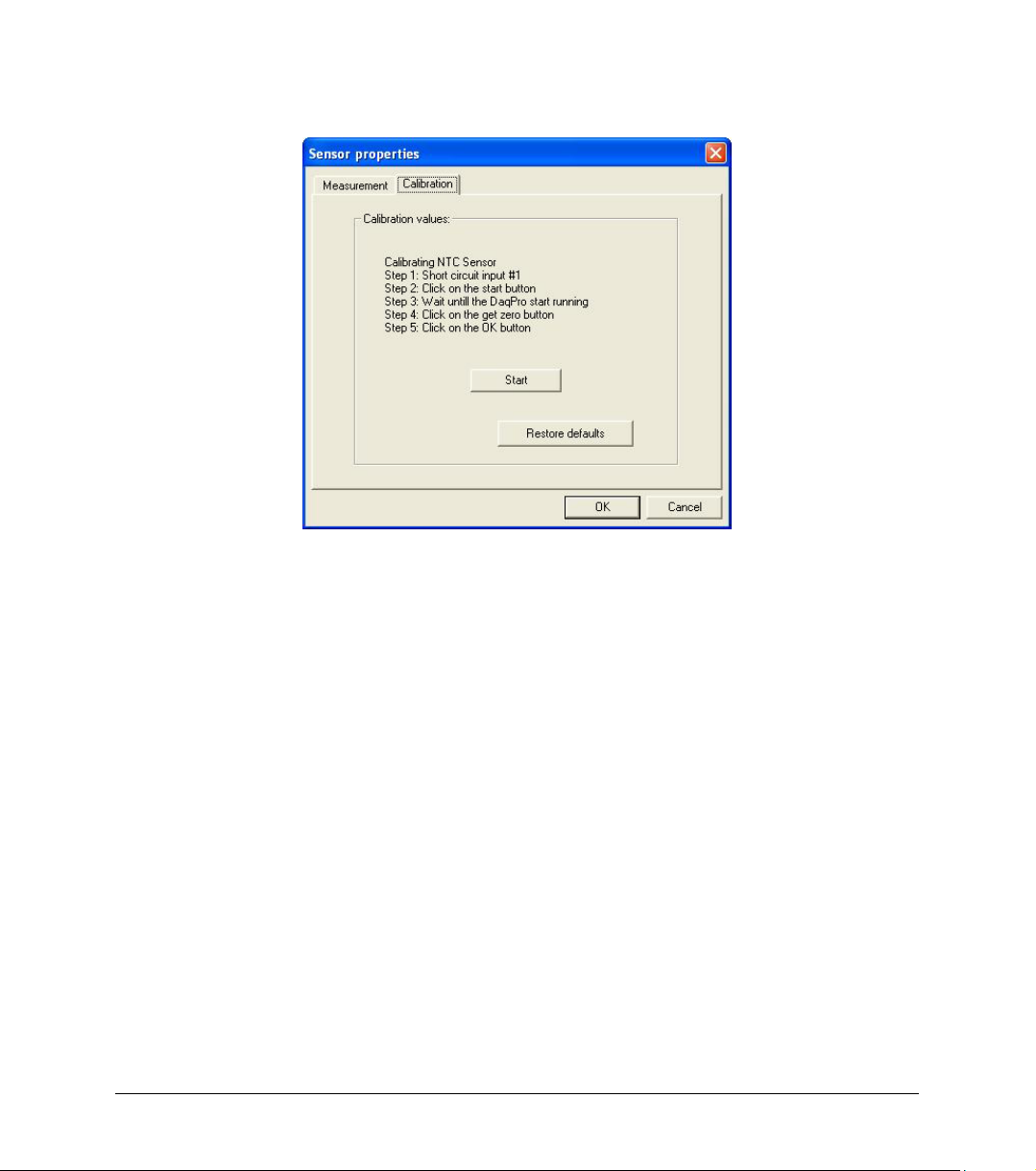
Figure 18: Zero calibration dialog

5. Click Restore defaults, then click OK

6. Repeat steps 1 to 4 above

7. Short circuit input 1

8. Click Start

9. Wait until OM-DAQPRO-5300 begins recording

10. Click Get zero

11. Click OK

The calibrated sensor parameters will be saved both in OM-DAQPRO-5300 and DaqLab memories, so
there is no need to calibrate OM-DAQPRO-5300 every time you run the DaqLab program.

68 Chapter 2 Working with DaqLab

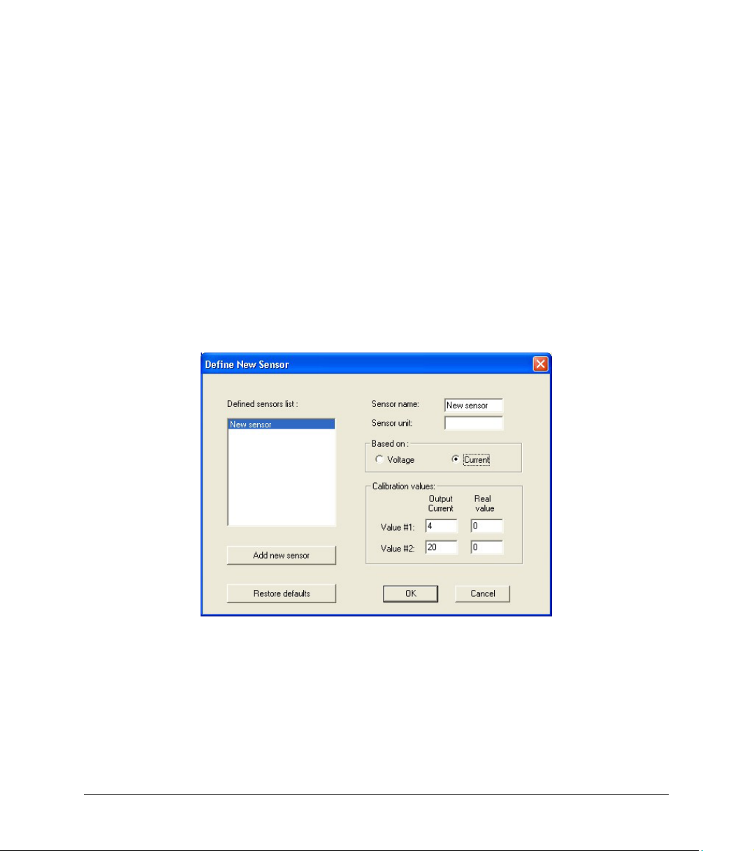
2.5.9. Define a Custom Sensor

DaqLab enables the user to define custom sensors. This is a useful tool for when OM-DAQPRO-5300 is
communicating with many sensors from different vendors.

Any additional sensor that you would like to connect to OM-DAQPRO-5300 must comply with the
following restrictions:

1) The sensor’s output must be either voltage in the range of 0 to 10V or current in the range of 4 to
24mA.

2) The sensor Transfer Function (sensor output voltage changes vs. the sampled phenomenon
changes) must be a linear Transfer Function.

To define a new sensor:

1. Connect OM-DAQPRO-5300 to the PC

2. Click Logger on the menu bar, then click Define new sensor to open
the Define new sensor dialog:

Figure 19: Define new sensor dialog

3. Click Add New Sensor

4. Select a Based on option (depending on whether your sensor’s
output is 0 to 10V or 4 to 24mA)

5. Type in a sensor name and a sensor unit

Chapter 2 Working with DaqLab 69

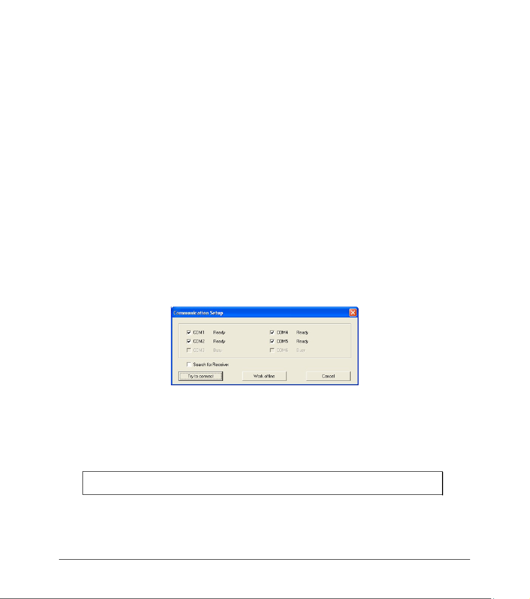
6. Type in two calibration values (two real values and the corresponding
output values of the sensor)

7. Click OK

OM-DAQPRO-5300 will send the definition to OM-DAQPRO-5300 and will add the new sensor to the
sensor list.

To use the custom sensor:

1. Plug the custom sensor into OM-DAQPRO-5300

2. Set up OM-DAQPRO-5300 using the Setup Wizard (see page 52) and
select the sensor from the sensor list next to the corresponding input

3. Proceed with the setup as you would normally do

2.5.10. Communication Setup

Communication between the PC and OM-DAQPRO-5300 takes place automatically whenever you send
a command to OM-DAQPRO-5300. However, the Communication Setup dialog can be used for more
advanced communication options.

1. Click Logger on the menu bar, and then click Com setup. DaqLab
will display a dialog reporting what COM Ports are already in use, and
which port is recommended for use with OM-DAQPRO-5300:

Figure 20: Communication setup dialog

2. Click Try to connect and DaqLab will try to communicate with OM-
DAQPRO-5300. If communication is achieved, DaqLab will designate
the selected port as OM-DAQPRO-5300’s communication port.

You can override the DaqLab recommendation and choose the COM Port yourself by clicking the check
box button to the left of the desired port, and clicking Try to connect.

Note: In case of any communication malfunction, please refer to the troubleshooting

guide on page 86.

70 Chapter 2 Working with DaqLab

3. You can click Work offline if you wish to work without OM-DAQPRO-

5300. While working offline, you can still open or import saved files to
view and analyze them

Chapter 2 Working with DaqLab 71

2.6. Analyze the data

2.6.1. Reading Data Point Coordinates

Position the cursor (see page 42) on a point to display its coordinates on the information bar at the
bottom of the graph window.

If more than one curve is displayed, and you want to read the Y coordinates of all of the curves
simultaneously, bring up digital meters (see page 48) for each of the curves. When you position a cursor
on one curve, the meters will show the corresponding Y-coordinates for the other curves.

2.6.2. Reading the Difference Between two Coordinate Values

Position one cursor on the first point and a second cursor on the second point to display the difference
between the two coordinate values on the information bar at the bottom of the graph window

2.6.3. Working with the Analysis Tools

The analysis tools can only be applied to data sets that are displayed in the graph window.

1. Use the cursors (see page 42) to select the graph and the data range
to which you want to apply the analysis.

2. Select the analysis function you wish to use.

The analysis function will be added onto the graph, with the exception of the smoothing (averaging)
function, which will replace the original data set.

2.6.4. Smoothing

The smoothing tool is very useful in reducing random "noises", especially if you want to apply any
analysis functions to the data. The smoothing process replaces every data point with the average of its
neighboring points.

1. Use the cursor to select the function on the graph that you want to
smooth

2. Click More smoothing

3. You can repeat the procedure to further smooth the data

72 Chapter 2 Working with DaqLab

on the graph toolbar

+

=

4. Click Less smoothing to reduce the amount of smoothing

2.6.5. Statistics

Use the statistics tool to display statistics of a selected data set or a range of data.

The statistics include:

Average – The average of all the numbers in the range

StDev. – The standard deviation

Minimum – The smallest value in the range

Maximum – The largest value in the range

Sum – Adds all the numbers in the range

Area – The area between the graph and the x-axis in the range

Samples – the number of data points in the range

Rate – the recording rate

To display statistics:

1. Use the cursors to select the graph and the data range to which you want to apply the
statistics

2. Click Analysis on the menu bar, then click Statistics

DaqLab will open a statistics window and will display the results in it

2.6.6. Most Common Analysis Functions

1. Linear fit

Click Linear Fit

and to display the line’s equation

Chapter 2 Working with DaqLab 73

on the main toolbar to draw a line of linear least square fit

baxy

=

Note: If you want the automatic curve fit equation to start at 0

before applying the linear fit (see page 82).

2. Derivative

Click Derivative
consecutive points on the source graph

3. Integral

Choose Integral from the Analysis menu to construct a graph in which each point is the integral of all
the preceding points on the source graph

on the main toolbar to construct a graph in which each point is the slope of the 3

t , apply the crop tool

2.6.7. The Analysis Wizard

1. Using the Analysis Wizard

The analysis wizard will guide you through the various analysis functions available in the DaqLab
program. The analysis functions are grouped into three main categories: curve fit (regression),
averaging, and mathematical and trigonometric functions.

To apply an analysis function to a data set:

1. Use the cursors to select the graph or data range to which you would
like to apply the analysis

2. Click Analysis Wizard on the main toolbar

3. Click a category tab:

a. Curve fit

b. Averaging

c. Functions

74 Chapter 2 Working with DaqLab

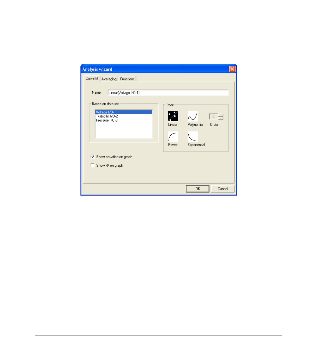
2. Curve fit

Figure 21: Analysis wizard – curve fit

1. Select a fit Type by clicking its icon (If you choose polynomial fit,
select the order you want)

2. If you use the cursor to select a data set, it will be highlighted in the
Based on data set list, but you have the option of selecting a different
data set

3. Type a name in the Name box (optional - the default name includes
both the function and the data set names)

4. Click the Show equation on graph check box to display the line’s
equation on the information bar

5. Click the Show R

2

on graph check box to display the correlation

coefficient on the information bar

6. Click OK

Chapter 2 Working with DaqLab 75

=

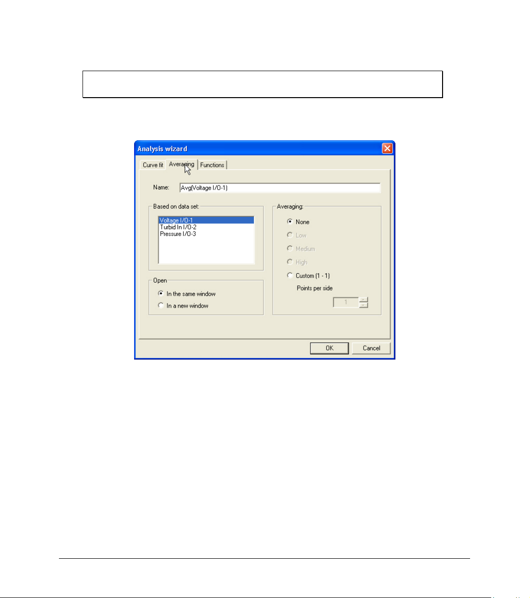
Note: If you want the automatic curve fit equation to start at 0

before any type of curve fitting (see page 82).

3. Averaging

Figure 22: Analysis wizard – averaging

1. If you use the cursor to select a data set, it will be highlighted in the
Based on data set list, but you have the option of selecting a different
data set

t , apply the crop tool

2. Select an averaging option (if you choose custom averaging, choose
the number of averaging points in the Points box)

3. Enter a name in the Name box (optional - the default name include
both the function and the data set names)

4. Select an Open option

5. Click OK

76 Chapter 2 Working with DaqLab

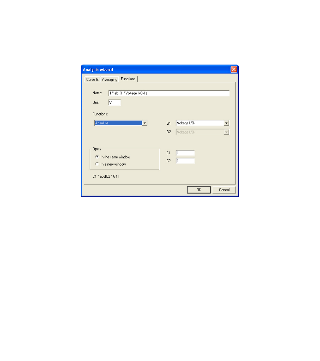
4. Functions

Figure 23: Analysis wizard – functions

1. Select a function from the Functions list. DaqLab displays the
function’s formula at the bottom of the dialog

2. If you use the cursor to select a data set, it will be highlighted in the
G1 drop list, but you have the option of selecting a different data set

3. If the analysis function involves two data sets, select the second data
set from the G2 drop list

4. Enter a constant in each of the C1 and C2 boxes (optional)

5. Enter a name in the Name box (optional – the default name includes
both the function’s formula and the data set name)

6. Enter a unit (optional)

7. Select an Open option

Chapter 2 Working with DaqLab 77

+

=

x

=

=

8. Click OK

2.6.8. Available Analysis Tools

This section includes a brief description of each of DaqLab’s analysis functions

1. Curve fit

a

n

bx

aey =

baxy

−L1

nn

10

axaxay +++=

n

Linear

Polynomial

Power

Exponential

DaqLab displays the curve fit equation and the correlation coefficient (R
the graph

2. Averaging

Draws a line of linear least square fit

Draws a line of polynomial least square fit (you must select an order between 1 and

6.)

y =

Draws a line of power least square fit

Draws a line of exponential least square fit

2

) on the information bar below

The average function replaces every point with the average of n neighboring points from both sides of
the point

Low averaging:

78 Chapter 2 Working with DaqLab

5=n , Medium averaging: 11

n , High averaging: 41

n

=

=

=

=

3. Functions

In the formulas below, G
can enter. The constant’s default value is 1

Absolute

Add

Arccosine

Arcsine

Average

and G2 represent selected data sets, and C1 and C2 are constants that you

1

GCCy =

121

Draws a line of the absolute values of a data set

GCGCy +

2211

Draws a line of the addition of two data sets

GCCy

Draws a line of the arccosine values of a data set (in radians). Arccosine is the angle

whose cosine is

Draws a line of the arcsine values of a data set in radians. Arcsine is the angle

whose sine is

·{average of C2 points around G1}

C

1

GC . The argument 12GC must be between –1 and 1.

12

GCCy

121

GC . The argument 12GC must be between –1 and 1.

12

)arccos(

121

)arcsin(

Cosine

Chapter 2 Working with DaqLab 79

Replaces every point with the averaging of C

)cos(

GCCy

121

Draws a line of the cosine values of a data set. The argument

expressed in radians.

neighboring points.

2

GC must be

12

−

=

Delta Y

tGGy

11

)0(

=

Derivative

Divide

Envelope
(lower)

Envelope
(upper)

Draws a line of the difference between the Y-coordinate of every point and Y­coordinate of the first point. Use this function to move the data set along the Y-axis
so that the point will intersect the Y- axis at the origin.

yy

−

nn

11

−+

y

=

n

Draws a line of the slopes of every three consecutive points of a data set. For high
recording rates and small ∆t, this line may be very noisy, which is why smoothing the
data set is recommended before applying the derivative function.

y =

Draws a line of the division of two data sets

Lower envelope of G

Draws a line that connects the minimum values of a data set. The tolerance defines
the minimum distance (in sampling points) between two minima, so that the envelope
function is able to ignore random "noises".

Upper envelope of G

t

∆

2

GC

11

GC

t

=∆

,

22

with tolerance of C1 points

1

with tolerance of C1 points

1

1

ratesampling

80 Chapter 2 Working with DaqLab

Draws a line that connects the maximum values of a data set. The tolerance defines
the minimum distance (in sampling points) between two maxima, so that the
envelope function will be able to ignore random "noises".

+

=

+

=

=

=

Exp.

eCy =

1

GC

12

Fourier
transform

Frequency

Integral

Linear

Ln

Draws a line of

Discrete Fourier transform of G

Draws a line of the amplitudes of the harmonics of Fourier transform vs. frequency.

The frequency of G1 (minimum of C

Draws a line of the frequency of a periodic data set vs. time. The constant C
the minimum data points in one cycle.

Draws a line in which each point is the discrete integral of all the preceding points in
a data set.

Draws a line of a linear displacement of a data set. This function is useful when you
want to change the point of origin of a data set.

e raised to the power of a data set.

.

1

points in one cycle).

1

tGCCy ∆∑

121

GCCy

121

)ln(

GCCy

121

defines

1

Log

Chapter 2 Working with DaqLab 81

Draws a line of the natural logarithm of a data set. The argument

positive.

)(log

GCCy

12101

Draws a line of the logarithm of a data set to base 10. The argument

positive.

GC must be

12

GC must be

12

=

=

=

=

Multiply

Reciprocal
(1/X)

Sine

Square (X

Square root

Subtract

2

GCGCy ⋅

2211

Draws a line of the multiplication of two data sets

C

1

G

1

)sin(

GCCy

121

GC must be

12

2

)( GCCy =

121

GCCy =

121

GC must be

12

GCGCy −

2211

y =

Draws a line of the reciprocal values of a data set.

Draws a line of the sine values of a data set. The argument

expressed in radians.

)

Draws a line of the squares of a data set.

Draws a line of the square root values of a data set. : The argument

greater than or equal to zero.

Tan

82 Chapter 2 Working with DaqLab

Draws a line the subtraction of two data sets.

)tan(

GCCy

121

Draws a line of the tangent values of a data set. The argument

expressed in radians.

GC must be

12

=

=

2.7. Special Tools

2.7.1. Crop Tool

The Crop tool enables you to trim the edges of a data set. Use it to remove unwanted data.

The time scale of the trimmed data is shifted so that it will start at

0

If you want the automatic curve fit equation to start at
curve fitting

After applying the crop tool, the trimmed data set replaces the original set on the graph display and a
new icon is added to the Data Map under cropped data.

1. To trim all data up to a point

1. Position a cursor (see page 42) on the data point

2. Click on the Graph menu, and then click Crop.

2. To trim all data outside a selected range

t , apply the crop tool before any type of

0

t .

1. Use the cursors to select the range you want to keep

2. Click on the Graph menu, and then click Crop.

Chapter 2 Working with DaqLab 83

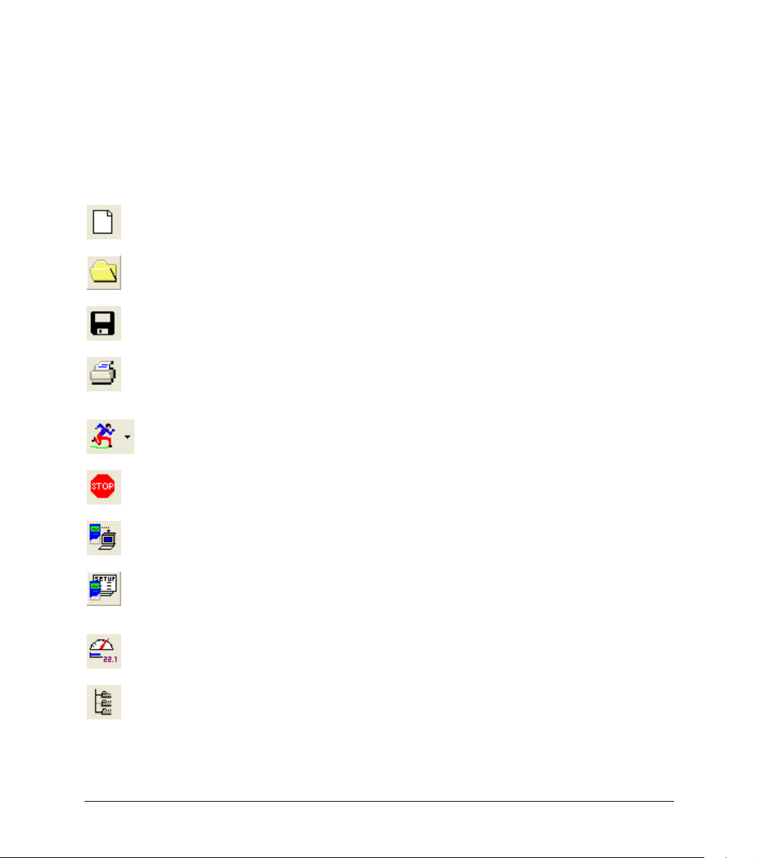
2.8. Toolbar Buttons

2.8.1. Main (upper) Toolbar

New

Open

Save

Print

Run

Stop

Download

Setup

Start new project

Open saved project

Save project

Select print options

Start a data recording session. Click on the down-arrow to select
recording mode

Stop recording

Download the data from the most recent recording session

Open the Setup dialog

Meter setup

Data map

84 Chapter 2 Working with DaqLab

Open the Meter setup dialog

Display the Data Map

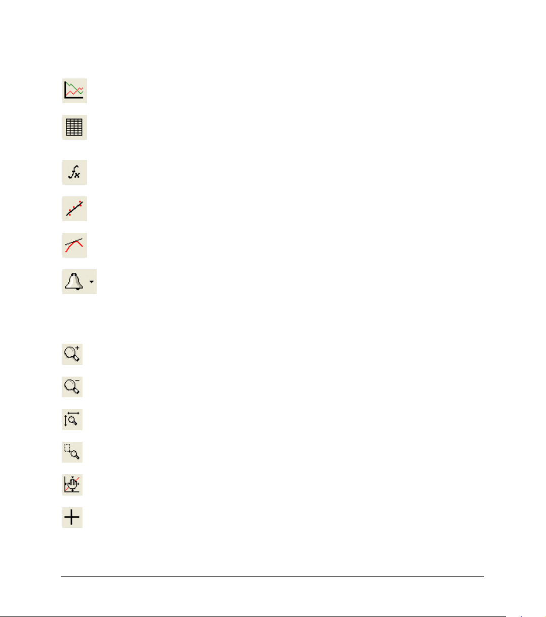
Graph

Table

Analysis

Linear fit

Derivative

Display alarm

Display the graph window

Display the table window

Open the Analysis wizard

Draw a line of linear fit of the selected data set

Draw a line of the derivative of the selected curve

Displays or removes alarm levels from the graph

2.8.2. Graph Toolbar

Zoom in

Zoom in around a selected point or in to a selected range

Zoom out

Autoscale

Zoom to selection

Pan

More smoothing

Chapter 2 Working with DaqLab 85

Reverse the most recent zoom operation

Display all the data

Zoom in to a selected area

Pan in all directions while in zoom mode

Smooth (average) the selected curve

Less smoothing

1st Cursor

nd

Cursor

2

Split graph

Edit graph

Graph properties

Add to project

Export to Excel

Reverse the most recent smoothing operation

Display or remove the first cursor

Display or remove the second cursor

Switch to a split graph display

Select the data to display on the axes

Graph formatting, scaling and units selection

Add the displayed graph to the project

Export the displayed graph to Excel

86 Chapter 2 Working with DaqLab

Chapter 3 Troubleshooting Guide

Symptom Cause of problem

I pressed the ON key on OM-DAQPRO­5300 and it did not turn on.

DaqLab was unable to connect to OM­DAQPRO-5300.

OM-DAQPRO-5300 and DaqLab
displays a warning message: “Illegal
sensor”

I downloaded “unexpected” data.

While running with an active trigger, OM­DAQPRO-5300 does not complete the
data logging.

• Try charging the battery, it may be weak.

• You are using an unsuitable AC/DC adaptor (see

page 15).

• The internal 3V disk battery is dead.

• OM-DAQPRO-5300 is turned off.

• The communication cable is not connected

properly.

• The communication cable is not connected to the

correct PC COM Port.

• There is no available Serial COM Port.

• OM-DAQPRO-5300 measured a voltage drop of

over 5V across an input that was selected as one
of the following types: 50mV, TCK, TCJ, TCT,
PT 100 or NTC.

• OM-DAQPRO-5300 measured a reversed voltage

drop of over -1V across an input that was selected
as one of the following types: 50mV, TCK, TCJ,
TCT or 10V.

• There may be up to 100 files stored in the OM-

DAQPRO-5300. Performing a “Download” means
loading one of them in sequential order. You have
probably loaded an old file accidentally. Try using
Selective download from DaqLab (see page 36)

• The trigger condition has not been fulfilled.

• The trigger condition was fulfilled, but the time

period was too short (less than 300µS).

Chapter 3 Troubleshooting 87

Symptom Cause of problem

I started a new logging and the data
logger stopped immediately afterwards.

The recorded data is “noisy”

OM-DAQPRO-5300’s memory is empty –
there are no stored files or notes.

• First check if the sampling rate was so fast that the

recording began and ended in less than a second.
If this is not the reason, recharge the 7.2V battery
and try again. OM-DAQPRO-5300 monitors the
battery power during the logging. If the battery
voltage is less then 5V, the logging is stopped
automatically.

• With voltage or current sensors, use short

connections between the circuit being tested and
the sensor.

• Avoid working near strong electromagnetic fields.

(e.g. engines, fluorescent lights)

• The internal 3V disk battery is dead.

88 Chapter 3 Troubleshooting

Chapter 4 Specifications

OM-DAQPRO-5300

Inputs

• 8 channel differential inputs

• Selectable type for each

input: 0-24mA, 0-50mV,
0-10V, NTC, PT-100,
Thermocouple, Pulse counter
(Input 1 only), frequency
(Input 1 only) and user
defined sensors

Input types

0 – 24mA

Range 0 to 24mA
Resolution 0.47µA
Accuracy ±0.5%
Loop impedance 21Ω
Maximum load 30mA, 5.2V

0 – 50mV

Range 0 to 50mV
Resolution 3µV
Accuracy ±0.5%
Input impedance 50MΩ
Maximum voltage 5.2V

0 – 10V

Range 0 to 10V
Resolution 200µV
Accuracy ±0.5%
Input impedance 125KΩ
Maximum voltage 25V

Temperature NTC-1

NTC – 10KΩ resistor
Range -25 to 150ºC
Resolution 0.05ºC
Accuracy ±0.5%

Temperature NTC-2

NTC – 2252Ω resistor
Range -25 to 150ºC
Resolution 0.05ºC
Accuracy ±0.5%

Temperature PT100

Range -200ºC to 400ºC
Resolution 0.1ºC (7mΩ)
Accuracy -200 – -50 ºC ±0.5%
50 – 400 ºC ±0.5%

-50 – 50 ºC ±0.5 ºC
Possible to connect up to 8
PT100 2 wires or 4 PT100 3
wires

Temperature thermocouple J

Range -200ºC to 1,200ºC
Resolution 0.1ºC (1µV)
Accuracy -200 – -50 ºC ±0.5%
50 – 1200 ºC ±0.5%

-50 – 50 ºC ±0.5 ºC
Cold junction compensation ±0.3ºC

Temperature thermocouple K

Range -250 to 1200ºC
Resolution 0.1ºC (1µV)
Accuracy -250 – -50 ºC ±0.5%
50 – 1200 ºC ±0.5%

-50 – 50 ºC ±0.5 ºC
Cold junction compensation ±0.3ºC

Temperature thermocouple T

Range -200 to 400ºC
Resolution 0.1ºC (1µV)
Accuracy -200 – -50 ºC ±0.5%
50 – 400 ºC ±0.5%

-50 – 50 ºC ±0.5 ºC
Cold junction compensation ±0.3ºC

Chapter 4 Specifications 89

Pulse counter (input 1 only)

Zero crossing detector
Opto coupler interface
Range 0 to 65,000 counts
Resolution 1 count
Frequency range 0 to 25Hz
Input signal 0 – 5V
Input impedance 470Ω

Frequency (input 1 only)

Zero crossing detector
Opto coupler interface
Range 20 to 4,000Hz
Time resolution 6.5µs
Input signal 0 – 5V
Input impedance 470Ω

Internal Temperature

NTC – 10KΩ resistor
Range -25 to 70ºC
Resolution 0.1ºC (1µV)
Accuracy ±0.3°C

General A to D specifications

Noise 30µV rms
Internal linearity error
±0.08% of FSR
Offset error 0.1%

Alarm output (output 8)

Open collector
Close position resistance 50Ω
Max. Load 50mA, 5V DC
Overload protection
50mA re-settable fuse

Communication

• USB 1.1 compliant

Sampling

• Capacity: 512KB

• Analog sampling rate:

Variable, 1 sample per hour
to 4,000 samples per
second, 1 channel

• Analog sampling resolution:
16 bits

• Channel separation 80dB

Man Machine Interface

• Full keyboard operation -
enables manual
programming of the Logger

• Graphic LCD 64x128 pixels

Power Supply

• Internal rechargeable 7.2V
Ni-MH battery

• Built in battery charger

• External 9V to 12V DC input

• Battery life: 40 hours

between charges

Operating Temperature Range

• 0 to 50°C

Casing

• Plastic ABS box

• Dimensions:

182×100×28 mm

• Weight: 450gr

Standards Compliance

• CE, FCC

DaqLab software

Main features

• Graphical, analysis WINDOWS based software for the OM-DAQPRO-5300

• Fast data download from the OM-DAQPRO-5300

• Data displayed in numeric or graphical display forms Graphical display of all inputs

90 Chapter 4 Specifications

• On-line retrieval and display of data in real-time

• Setup wizard for the OM-DAQPRO-5300

• Define of up to 20 new sensor in the OM-DAQPRO-5300

Read the defined sensor’s units on the logger’s display

• Full calibration of the OM-DAQPRO-5300 via software

• Documentation and filing

• Alarm levels on graphs

• Export and import to and from spreadsheets

• More than 30 analytical function, for professional analysis of the collected data

System requirements

Software

 Windows 98 or later

 Internet Explorer 5.0 or later (you can install Internet Explorer 5 when you install

DaqLab, since it ships with the product)

Hardware

 Pentium 200MHz or higher

 32 MB RAM (64 MB recommended)

 10 MB available disk space for the DaqLab application (50 MB to install the supporting

applications

Chapter 4 Specifications 91

Appendix: Figures

Figure 1: OM-DAQPRO-5300 external connections................................................................................ 10

Figure 2: OM-DAQPRO-5300’s inputs block terminal ............................................................................. 12

Figure 3: connecting 3 wire PT 100.........................................................................................................13

Figure 4: connecting external alarm device ............................................................................................. 14

Figure 5: OM-DAQPRO-5300 front panel................................................................................................ 16

Figure 6: Frequency Aliasing................................................................................................................... 29

Figure 7: DaqLab window layout .............................................................................................................34

Figure 8: Edit graph dialog ......................................................................................................................45

Figure 9: Setup wizard step 1 of 3........................................................................................................... 52

Figure 10: Setup wizard step 2 of 3......................................................................................................... 53

Figure 11: Setup wizard step 3 of 3......................................................................................................... 54

Figure 12: alarm settings.........................................................................................................................55

Figure 13: X-axis properties dialog..........................................................................................................57

Figure 14: Triggering dialog.....................................................................................................................58

Figure 15: Edit notes dialog..................................................................................................................... 60

Figure 16: Two-point calibration dialog.................................................................................................... 63

Figure 17: Offset calibration dialog..........................................................................................................65

Figure 18: Zero calibration dialog ............................................................................................................ 67

Figure 19: Define new sensor dialog ....................................................................................................... 68

Figure 20: Communication setup dialog ..................................................................................................69

Figure 21: Analysis wizard – curve fit ...................................................................................................... 74

Figure 22: Analysis wizard – averaging ................................................................................................... 75

Figure 23: Analysis wizard – functions.....................................................................................................76

92 Appendix

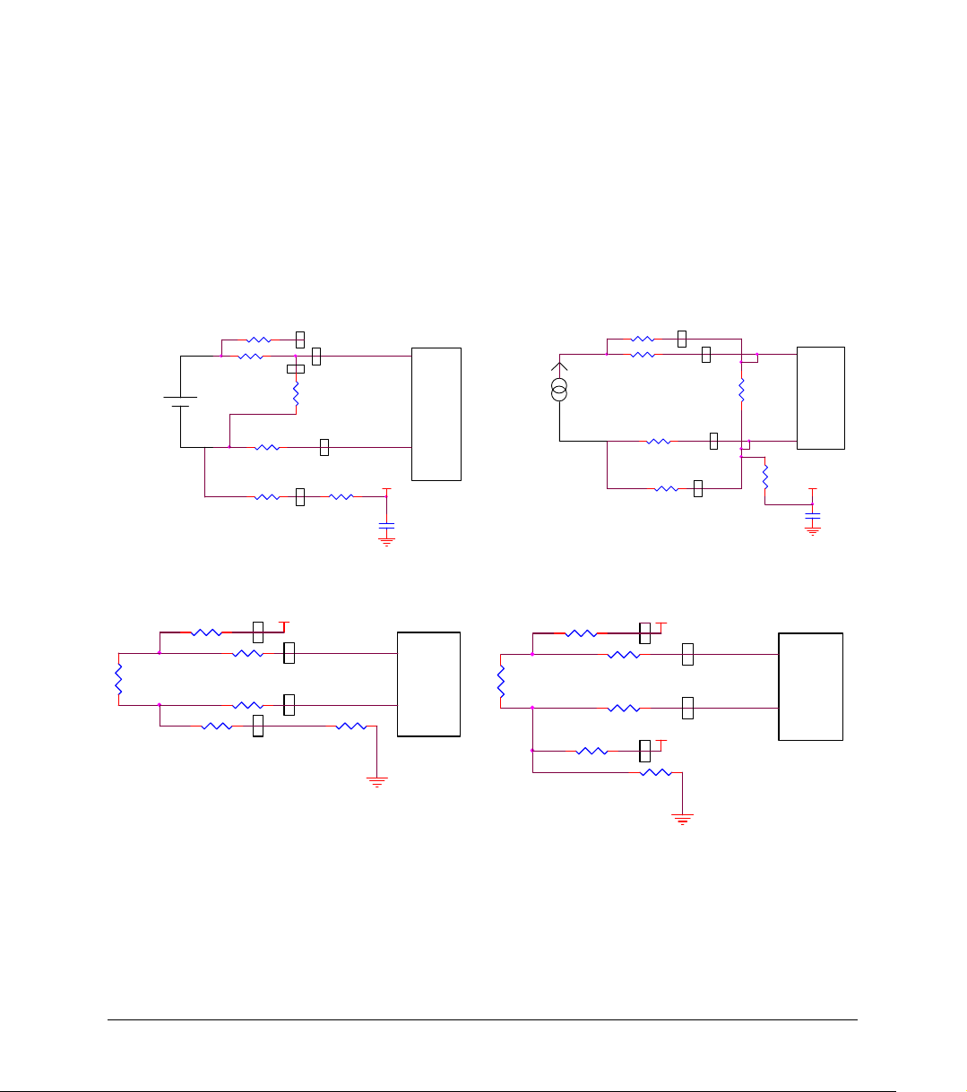
Appendix:
Simplified measurement circuits

0 to 10V 0 to 24mA

100K

80R

21R

100K

80R

100R

ADC

VREF

1UF

0-10V

100K

80R

100K

80R

25K

100R

ADC

VREF

1UF

0-24mA

2 wire PT 100 3 wire PT 100

PT100

80R

100K

100K

80R

2 Wire PT100

100uA

10k

80R

PT100

ADC

80R

100K

100K

100uA

ADC

100uA

3 Wire PT100

4.7k

Appendix 93

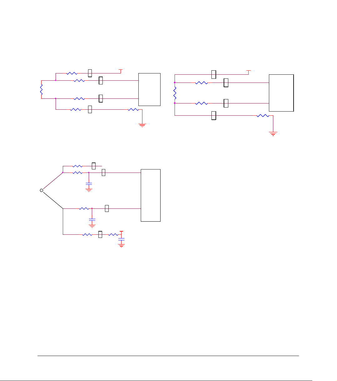
NTC Internal NTC

80R

20uA

20uA

NTC 10K

NTC

Thermocouple

100K

Thermocouple

80R

80R

100K

100K

100K

80R

1UF

1UF

100R

VREF

1UF

10k

ADC

ADC

NTC 10K

100K

100K

ADC

10k

Internal NTC

94 Appendix

Index

A

AC/DC adaptor · 15
alarm · 45

level · 13
output · 14, 55
set · 13
setup · 54

analysis · 71

averaging · 75
carve fit · 74
derivative · 73
function · 76
integral · 73
smoothing · 71

wizard · 73
autoscale · 43
averaging · 75

B

battery · 15

level · 56
block terminal · 12

C

cable · 9
calibration · 15, 61
channels · 11
chart · See table
clear

data · 50

memory · 59

clock

internal · 27
COM port · 69
comment · 15, 59
communication · 69
configuration · 26
connect · 69
connection

3 wire PT 100 · 12

frequency/pulse counter ·

12
polarity · 12
screw terminal · 12
to a computer · 11

continuous · 29, 30
contrast · 27
coordinates · 25, 42
copy · 51
counter · 12
crop · 82
cursor · 25, 42
curve fit · 72, 74

D

data map · 49
define

custom sensor · 68

delayed start · See

triggering

delete · 50
derivative · 73
display

control the display · 49
data map · 49
graph · 41
meters · 48
options · 41

properties · 56
select · 20
table · 47

download · 36, 37

E

edit

graph · 44

notes · 60
enter · 19, 22
escape · 22
event · 14
event recording · 58
Excel · 51
export · 51
external power · 11

F

filter · 26, 55
format

graph · 46

table · 48
frequency · 12
functions · 76

G

getting started · 35
graph · 24, 41

Index 95

I

icon · 22
Illegal sensor · 13
import · 38
input · 11
integral · 73

K

keypad · 16

L

layout

DadPRO · 16
DaqLab · 34

load

last setup · 25
notes · 60

low pass filter · 26, 55

M

mains adaptor · 15
manual

sampling · 29

memory · 30

clear · 27, 59
menu · 21
meter · 23, 48

N

noise · 27, 56
notes · 60
number

format · 46, 48
of samples · 19, 22, 54

O

online

communication · 36
open · 37
output · 14, 55

P

panel · 16
panning · 44
Password · 62
polarity · 12
power · 11
preset · 56
print

graph · 39

taple · 40
program

DaqPRO · 52
programming

rules · 30
project · 33, 38
properties

graph · 46

table · 48
PT 100

3 wire · 12
PT 100 · 12
pulse · 12

R

rate · 19, 22, 28, 30, 53, 87
recharge · 15
recording

data · 21, 35
options · 36
rate · See rate
start · 59
stop · 59

time · 19, 22, 54
regression · See curve fit
requirements · 31
run · 35, 59

S

sampling Points · 29
sampling rate · See rate
save · 37
scale · 43
screen contrast · 27
scroll · 53
sensor · 11, 12, 17

assign to input · 52

calibration · 61

custom · 68

plug in · 17
serial number · 15
setup · 18, 22, 25, 28, 52
slope · See derivative
smoothing · 71
specifications · 88
spreadsheet · 51
stand alone · 16
start · 20, 22, 35
stop · 21, 22, 35
system configuration · 26

T

table · 23, 47
temperature

units · 27, 60
terminal · 12
timer delay · 58

96 Index

toolbar

graph · 84

main · 83
triggering · 57
trim · See crop
troubleshooting · 86

U

units

format · 46, 48

temperature · 27

V

value · 25, 42
view · 41

W

wizard

analysis · 73
setup · 52

X

X-axis · 45, 57

Y

Y-axis · 41, 45

Z

zoom · 25, 42

Index 97