Omega D2000 User guide

omega.com

e-mail: [email protected]

For latest product manuals:

omegamanual.info

User’s Guide

D2000 Series

Digital Transmitters

MADE IN

Shop online at

Servicing North America:

U.S.A.: One Omega Drive, Box 4047

ISO 9001 Certified Stamford, CT 06907-0047

Tel: [phone] FAX: [phone]
e-mail: [email protected]

Canada: 976 Bergar

Laval (Quebec) H7L 5A1, Canada
Tel: [phone] FAX: [phone]
e-mail: [email protected]

For immediate technical or application assistance:

U.S.A. and Canada: Sales Service: 1-800-826-6342 / 1-800-TC-OMEGA

®

Customer Service: 1-800-622-2378 / 1-800-622-BEST

®

Engineering Service: 1-800-872-9436 / 1-800-USA-WHEN

®

Mexico: En Espan˜ol: [phone]-7803 e-mail: [email protected]

FAX: [phone] [email protected]

Servicing Europe:

Benelux: Postbus 8034, 1180 LA Amstelveen, The Netherlands

Tel: [phone] FAX: [phone]
Toll Free in Benelux: 0800 0993344
e-mail: [email protected]

Czech Republic: Frystatska 184, 733 01 Karvina´, Czech Republic

Tel: [phone] FAX: [phone]
Toll Free: 0800-1-66342 e-mail: [email protected]

France: 11, rue Jacques Cartier, 78280 Guyancourt, France

Tel: [phone] FAX: [phone]
Toll Free in France: 0800 466 342
e-mail: [email protected]

Germany/Austria: Daimlerstrasse 26, D-75392 Deckenpfronn, Germany

Tel: [phone] FAX: [phone]
Toll Free in Germany: 0800 639 7678
e-mail: [email protected]

United Kingdom: One Omega Drive, River Bend Technology Centre

ISO 9002 Certified Northbank, Irlam, Manchester

M44 5BD United Kingdom
Tel: [phone] FAX: [phone]
Toll Free in United Kingdom: 0800-488-488
e-mail: [email protected]

OMEGAnet®Online Service Internet e-mail

omega.com [email protected]

It is the policy of OMEGA Engineering, Inc. to comply with all worldwide safety and EMC/EMI
regulations that apply. OMEGA is constantly pursuing certification of its products to the European New
Approach Directives. OMEGA will add the CE mark to every appropriate device upon certification.

The information contained in this document is believed to be correct, but OMEGA accepts no liability for any
errors it contains, and reserves the right to alter specifications without notice.
WARNING: These products are not designed for use in, and should not be used for, human applications.

Omega Engineering
One Omega Drive
P O Box 4047
Stamford, CT 06907
Phone: 1-800-DAS-IEEE
Fax: [phone]
e-mail: [email protected]
www.omega.com

D2000 SERIES
PROGRAMMING MANUAL

REVISED 10/27/04

TABLE OF CONTENTS

CHAPTER 1 Linear Scaling 1-1

Nonlinear Functions 1-3

CHAPTER 2 Block Diagram 2-2

Programming Table 2-3
Breakpoints 2-7

CHAPTER 3 BreakPoint Command 3-1

MiNimum Command 3-2
MaXimum Command 3-2

CHAPTER 4 Programming Software 4-1

General Guidelines 4-1
Function Programming 4-4
Linear Scaling 4-7

CHAPTER 5 Programming Steps 5-3

Examples 5-6

Chapter 1

Introduction

The D2000 series of intelligent analog-to-computer interfaces are designed
to solve many difficult interfacing problems that cannot be performed with
existing standard interfaces. The D2000 series may be programmed to
create custom transfer functions to interface to non-standard sensors or to
scale the outputs to any engineering units desired.

The D2000 series is an enhancement of the D1000 series of standard
interfaces. The D2000 series is similar to the D1000 series in every respect
except that the D2000 interfaces allow custom input-to-output transfer
functions. As shipped from the factory, the D2000 modules operate in the
same manner as their D1000 counterparts. For example, a D2111 shipped
from the factory contains the same transfer function as a D1111 module; in
this case they are both ±100 mV inputs and communicate with RS-232.
Before any attempt is made to program a D2000, you must first be familiar
with the operation of a D1000 module as described in the D1000 manual.

The D2000 contains built-in commands to create custom functions. All
programming is performed through the communications port of the D2000
module. There is never any need to open the module case. Modules may be
re-ranged remotely as many times as desired. Transfer function data values
are stored in nonvolatile memory to retain the scaling even if power is
removed.

Linear Scaling

The basic concept of the D2000 series is to create interfaces which output
data in application specific engineering units that may be instantly read and
interpreted without any data conversion necessary by a host computer. In
fact, the D2000 interfaces may be used with a dumb terminal to provide data
readings in easy-to-understand engineering units. For example, a typical
pressure sensor might provide a 1 to 5V. linear output for pressures of 0 to
1000 psi. Using a D1131 module or an unprogrammed D2131 unit the output
data would look like this:

Pressure (psi) Sensor Output D2131 Output (mV)
0 1V +01000.00

500 3V +03000.00
1000 5V +05000.00

The standard output of the D2131 reads out in units of millivolts. Even though
the D2131 will faithfully output the sensor voltage, the real parameter of
interest is pressure, not voltage, and the voltage readings may be difficult to

Introduction (1-2)

interpret. To make the output data more readable, the D2131 may be
programmed to output the data values in units of pressure:

Pressure (psi) Sensor Output D2131 Output (psi)
0 1V +00000.00

500 3V +00500.00
1000 5V +01000.00

In some cases, the desired output may be more specific to a particular
application. Assume that the same pressure sensor is used to measure the
“fullness” of a pressure vessel, such as a cylinder of compressed air. The
D2131 could be scaled to output in units of “percent” and in this case we will
assume that if the cylinder reads 750 psi it is 100% full:

Pressure Volts Output (%)
0 1 +00000.00

375 2.5 +00050.00
750 4 +00100.00

Nonlinear Functions

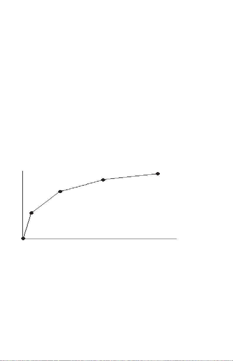
Figure 1 Piece-wise Linear Approximation.
As we have shown with the linear pressure sensor example, the output may

be scaled to any units we desire. However, the real power of the D2000
series is that they may be programmed to provide a nonlinear transfer
function. This capability may be used to provide outputs in engineering units
for nonlinear sensors. The D2000 uses a linear piece-wise approximation
technique to describe nonlinear functions. Up to 24 linear segments may be
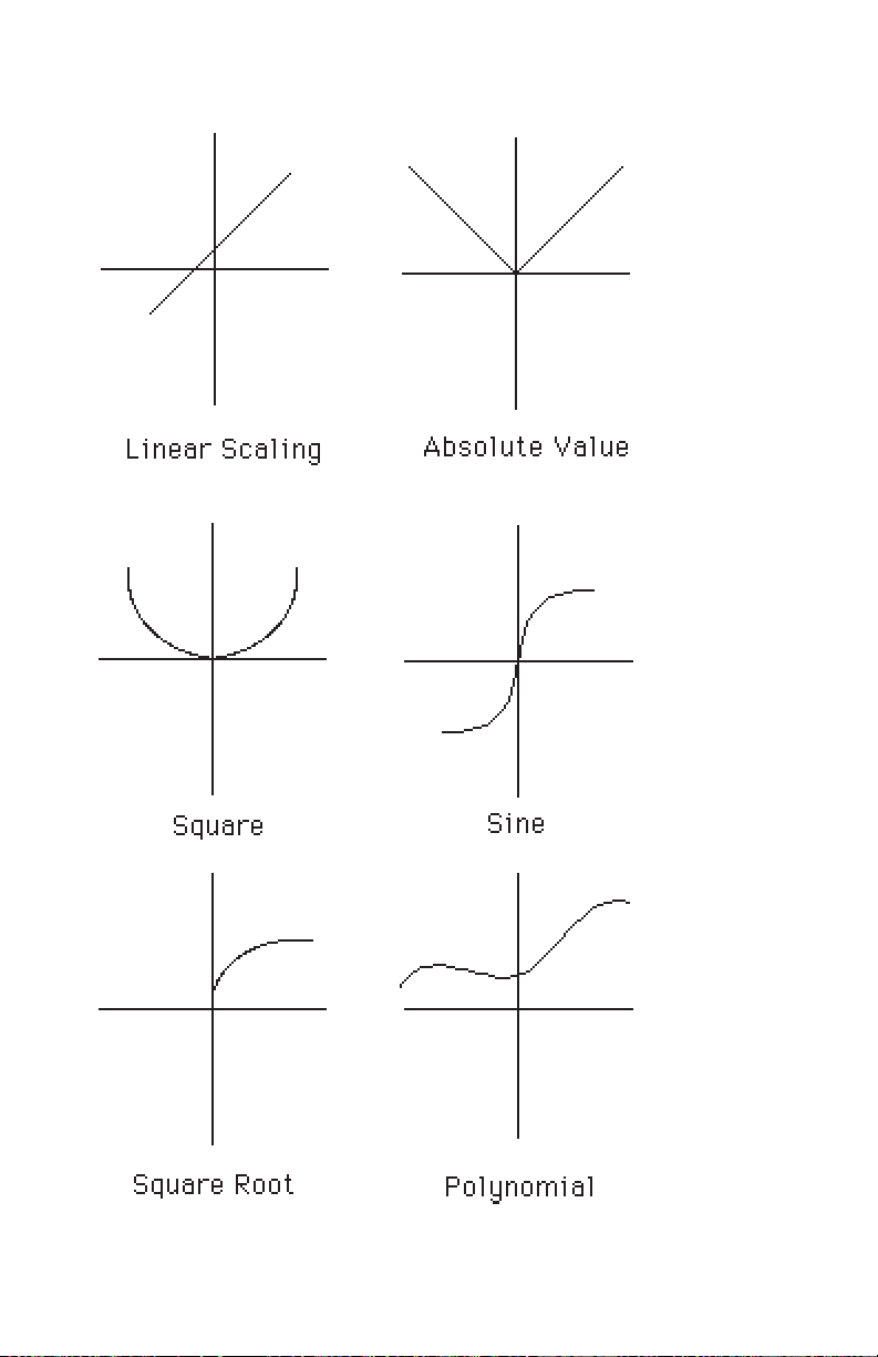
used to approximate a function, as shown in Figure 1. Figure 2 shows some
of the variety of curves that may be programmed into the D2000.

The D2000 modules may also be programmed in the field to specific test
inputs where the actual nonlinearity is not known.

Introduction (1-3)

Figure 2 Example Curves.

Introduction (1-4)

Chapter 2

Theory of Operation

The D2000 performs all scaling functions in firmware using the module’s
internal microprocessor. All scaling and nonlinear function data is stored in
a table contained in EEPROM nonvolatile memory. Scaling data stored in
the memory will remain intact indefinitely even if power is removed. D2000
modules may be re-scaled up to 10,000 times.

All re-scaling operations are performed with simple commands given to the
module through its communications port. The D2000 series command set
encompasses all the the D1000 commands plus additional commands to
perform function programming. There is no need to open or have access to
the module to perform re-scaling. In many cases the modules may be re­scaled remotely after they have been installed. Detailed descriptions of the
D2000 programming commands are given in Chapter 5.

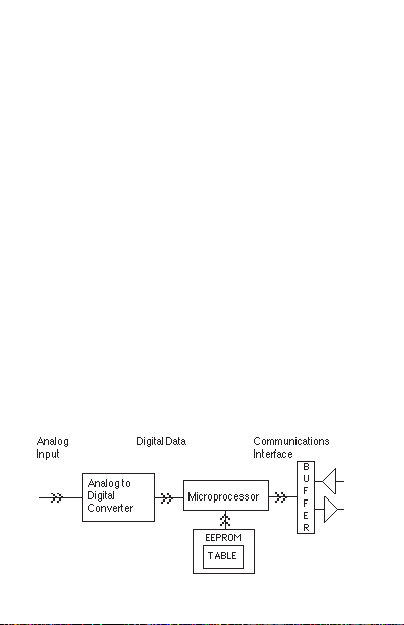
Figure 3 is a simplified block diagram of the D2000, showing only the
portions related to re-scaling. The µP reads the raw Analog-to-Digital
Converter (ADC) data after every conversion. The µP takes the raw ADC
data and looks it up in a table held in EEPROM. The table contains entries
which map the raw ADC data to user-defined output data values scaled in
engineering units. If an exact match is not found, the data is interpolated
between the two closest table entries. The resulting data in engineering units
is stored in a memory buffer where it may be read by the Read Data (RD)
or New Data (ND) Commands.

Note that the re-scaling operation acts on the output of the analog-to-digital
converter. The basic input-to-output transfer function of the ADC is fixed and
cannot be changed. For example, a D2131 module with a ±5V input range
cannot be re-scaled to ±10V or any other range. Analog input scaling is
performed by selecting the D2000 model that best matches the sensor
signal. The ADC data is then manipulated with the function table to provide
output data in engineering units.

Figure 3. D2000 Series Block Diagram

Programming Table

Theory of Operation (2-2)

Figure 4 shows a programmer’s model of the table used to program the
input-output transfer function of the D2000. The table values are inten­tionally left blank so that it may be copied and used as a worksheet to
help program the modules.

ANALOG DATA

INPUT OUTPUT
MINIMUM X
MAXIMUM X
BREAKPOINT ØØ X
BREAKPOINT Ø1 X
BREAKPOINT Ø2 X
BREAKPOINT Ø3 X
BREAKPOINT Ø4 X
BREAKPOINT Ø5 X
BREAKPOINT Ø6 X
BREAKPOINT Ø7 X
BREAKPOINT Ø8 X
BREAKPOINT Ø9 X
BREAKPOINT ØA X
BREAKPOINT ØB X
BREAKPOINT ØC X
BREAKPOINT ØD X
BREAKPOINT ØE X
BREAKPOINT ØF X
BREAKPOINT 1Ø X
BREAKPOINT 11 X
BREAKPOINT 12 X
BREAKPOINT 13 X
BREAKPOINT 14 X
BREAKPOINT 15 X
BREAKPOINT 16 X

MIN

MAX

ØØ

Ø1

Ø2

Ø3

Ø4

Ø5

Ø6

Ø7

Ø8

Ø9

ØA

ØB

ØC

ØD

ØE

ØF

1Ø

11

12

13

14

15

16

Y

MIN

Y

MAX

Y

ØØ

Y

Ø1

Y

Ø2

Y

Ø3

Y

Ø4

Y

Ø5

Y

Ø6

Y

Ø7

Y

Ø8

Y

Ø9

Y

ØA

Y

ØB

Y

ØC

Y

ØD

Y

ØE

Y

ØF

Y

1Ø

Y

11

Y

12

Y

13

Y

14

Y

15

Y

16

Figure 4. Breakpoint Table.

Theory of Operation (2-3)

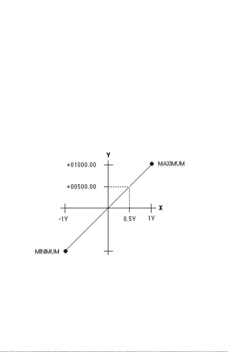
The two most important points in the table are the Minimum and Maximum
points. These two table entries specify the minimum and maximum end­points of the transfer function curve. For instance, a D2121 has a range of
±1V, and the standard table values are:

Analog Input Data Output

Minimum -1V -01000.00
Maximum +1V +01000.00

Plotted on a graph (Figure 5), these two points specify the endpoints of the
transfer curve. In this case, the analog input variable X is in terms of voltage.
The X values in the table specify the minimum and maximum voltages that
may be applied to the analog input that will result in a linearized output. (The
X voltage values are actually stored in memory in terms of ADC binary data).
Voltage values applied to the analog input that are more negative than Xmin
will result in an overload output of -99999.99. Similarly, voltage values
greater than Xmax will result in +99999.99.

Figure 5. Function Endpoints

The corresponding Y values in the table specify the output data of the
minimum and maximum points. In this case, a -1V input corresponds to an
output of -01000.00mV. The Y values are always stored in the standard data
format of sign, 5 digits, decimal point and two additional digits.

The minimum and maximum points are the only table values necessary to
specify a linear transfer function. For analog input values between Xmin and
Xmax, the output values are determined by linearly interpolating between
the minimum and maximum points. For instance, in the case of the D2121,

Theory of Operation (2-4)

an analog input value of +.5V is linearly interpolated to an output value of
+00500.00 (Figure 5).

It should be apparent at this point that a D2000 module may be re-scaled by
modifying the minimum and maximum values in the table. This may be
accomplished by using the Minimum (MN) command and the Maximum
(MX) command. Using the D2121 ±1 volt module as an example, we may
use the MN and MX commands to alter the table to look like this:

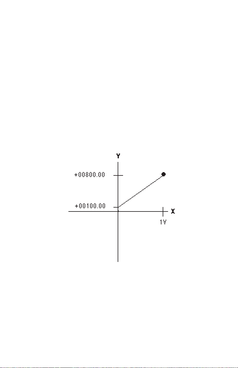
Analog Input Data Output

Minimum 0V +00100.00
Maximum +1V +00800.00

In this case the minimum point is 0V, corresponding to the output data
+00100.00. The maximum point is +1V input and +00800.00 output. The
graph of this equation is shown in Figure 6.

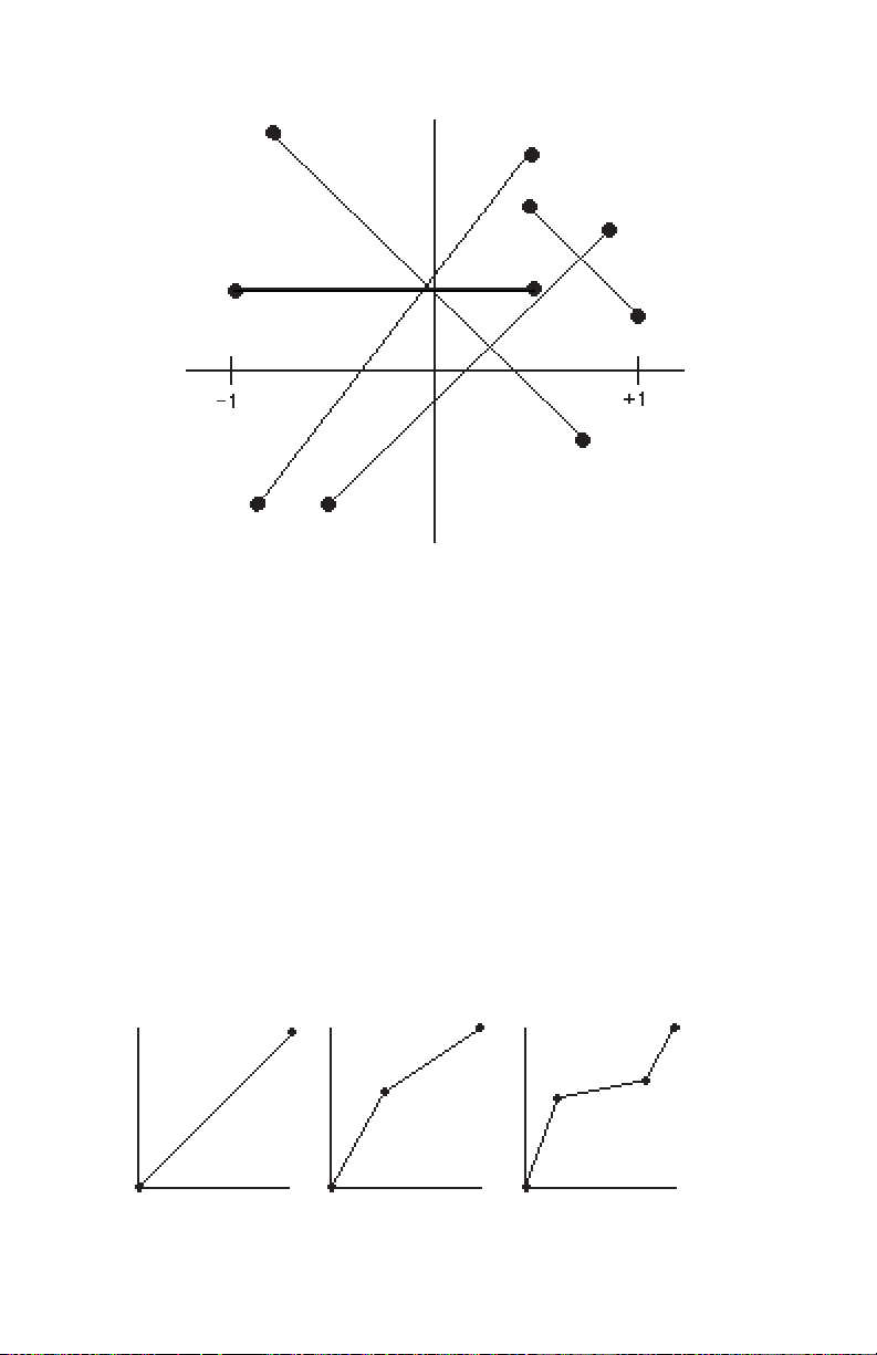
By changing the minimum and maximum values in the table, an infinite

Figure 6

number of linear functions may be specified, bounded by X values of ±1V
and Y values of ±99999.99. Figure 7 shows a few possibilities.

The exact procedure necessary to program the maximum and minimum
points is described in Chapter 5.

Theory of Operation (2-5)

Figure 7. Examples of Linear Functions.

Breakpoints

From Figure 4, we can see that most of the transfer function table is reserved
for “Breakpoints”. Breakpoints are used to modify the basic linear curve
defined by the Minimum and Maximum points to create nonlinear functions.

Nonlinear functions in the D2000 are approximated by using linear seg­ments which are specified by the data values held in the Breakpoint Table.
Up to 23 breakpoints may be programmed to specify up to 24 linear
segments. Figure 8 illustrates the action of the breakpoints. Figure 8a shows
a basic linear transfer function described by the Minimum and Maximum
points. Figure 8b shows the effect of one breakpoint used to modify the linear
function. Notice that the breakpoint has created a nonlinear function
described by two linear segments joined at the breakpoint. Figure 8c shows
that two breakpoints may be used to specify a nonlinear curve described by
three linear segments. Up to 23 breakpoints may be used to create complex
nonlinear curves.

abc

Figure 8. Breakpoint Examples

Theory of Operation (2-6)

Breakpoints are stored in the EEPROM table in the same fashion as the
minimum and maximum points. Each breakpoint is described by an X-Y pair
specifying the analog input value at which the breakpoint occurs and the
corresponding output data value. When the microprocessor reads the
analog (X) data from the ADC, it searches the breakpoint table to find the X
value closest to the input data. The micro then linearly interpolates between
two breakpoints to calculate the resulting output data.

Any number of breakpoints up to 23 values may be specified. The breakpoint
table must be filled progressively starting with Breakpoint 00 to Breakpoint
16 (hex). Unused or “erased” breakpoints are not used in the function
calculation.

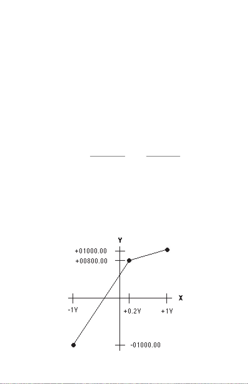
Let’s use the D2121 ±1V module again as an illustrative example to show
the effect of a breakpoint. Figure 9 shows the D2121 function table with 1
breakpoint programmed:

Analog Input Data Output
Minimum -1V -01000.00
Maximum +1V +01000.00
Breakpoint 00 +0.2V +00800.00
Breakpoint 01 - - - - - - - - - - - - ­……………
……………

Breakpoints 01 through 16 (hex) are erased and do not enter the function
calculation. The Minimum and Maximum table entries contain the standard
data values of ±01000.00mV. The new curve is shown in Figure 9.

Figure 9

Theory of Operation (2-7)

Notice how the breakpoint has affected the whole curve, creating a nonlinear
function. Here are a few samples of the input-output values that may be
obtained from this curve:

Analog Input Data Output

-.8V -00700.00

-.6V -00400.00

-.4V -00100.00

-.2V +00200.00

0V +00500.00

+.2V +00800.00

+.4V +00850.00

+.6V +00900.00

+.8V +00950.00

The procedure to create a breakpoint table is detailed in Chapter 4.

Chapter 3

Command Set

D2000 COMMAND SET

The D2000 module series incorporates the same command set as the
D1000 series, with new commands added to facilitate custom range
programming. The added D2000 commands are used only for program­ming. For normal operational commands, refer to the D1000 manual.

CAUTION: THE D2000 PROGRAMMING COMMANDS MUST BE USED
WITH CARE. EACH OF THE COMMANDS IS CAPABLE OF DESTROY­ING FACTORY CALIBRATION.

All of the commands added to the D2000 series are write-protected to guard
against accidentally altering data values stored in the module’s EEPROM.
Therefore, all programming commands must be preceded with a Write
Enable (WE) command.

All of the D1000 command-response protocol rules apply to the D2000.
This section is intended only to describe the new commands. For program-

ming information refer to Chapter 5.

BREAK POINT (BP)

Nonlinear functions may be approximated in the D2000 by describing the
function curve with a series of line segments (see Figure 1). The line
segments are programmed into the D2000 using the BreakPoint (BP)
command. A breakpoint specifies the intersection between two linear
segments used to approximate the nonlinear transfer function. Up to 23
breakpoints may be used to specify 24 linear segments in a curve.

To program a breakpoint, a known analog stimulus must be applied to the
sensor input of the D2000 module. This specifies the input variable (X-axis)
location of the breakpoint. The corresponding output data (Y-axis) of the
breakpoint is specified as an argument to the BreakPoint (BP) command.

Example: (Spaces have been added to the command for clarity)

Command: $1 BP 03 +00100.00
Response: *

Command: #1 BP 03 +00100.00
Response: *1BP 03 +00100.00FA (FA = checksum)

The first two characters following the “BP” command specify the breakpoint
number. Up to 23 breakpoints may be programmed into the D2000. In the
sample command above, breakpoint number “03” is being specified. Break­point numbers are expressed in two-digit hexadecimal notation, ranging
from “00” to “16” for a total of 23 (decimal) points. During a normal

Command Set (3-2)

programming operation, breakpoints are entered in sequence in progres­sively-increasing X values starting from the minimum value (see Minimum
(MN) command). Breakpoint programming must start with Breakpoint “00”.
It is not necessary to specify all the breakpoints; any number up to 23 may
be used. However, a breakpoint sequence must start at “00” and be entered
sequentially. Any remaining breakpoints may be left unspecified.

Following the breakpoint number, the output (Y-axis) data must be speci­fied. The data must be in standard D1000 format: sign, five digits, decimal
point, 2 digits. The output data specifies the module’s output response for
the test stimulus applied to the module input.

Before setting the breakpoints with the BreakPoint (BP) Command, the
overall function span must be specified by the MiNimum (MN) and MaXi­mum (MX) commands. (See Chapter 5 for programming instructions.)

Erase Breakpoints (EB)

The EB command erases all previously entered breakpoints from the
module’s EEPROM. Erased data cannot be recovered. Therefore, before
using the EB command, be prepared to re-program all of the breakpoints in
the unit. The S1000 Utility Software can be used to save factory calibration
data values. The EB command is used to provide a clean slate before
entering a new breakpoint sequence. Previous end-point data entered by
the MiNimum (MN) and MaXimum (MX) commands are not affected.

Command: $1EB
Response: *

Command: #1EB
Response: *1EBE2 (E2 is the checksum)

MiNimum (MN)

The MiNimum (MN) command is used to define an endpoint of a transfer
function programmed into a D2000 module. The minimum endpoint defines
the most negative value allowed on the analog input before an overload will
occur.

In effect, the minimum value is the starting breakpoint in a programmed
transfer function. To use the MiNimum (MN) command, a known analog test
stimulus must be applied to the analog input of the module. The test stimulus
must correspond to the most negative value of the desired analog input
range. The analog input stimulus specifies the starting input value (X-axis)
of the transfer function. The test input must lie within the factory-specified full

Command Set (3-3)

scale input range of the module.
The argument of the MN command specifies the starting output value (Y-

axis) of the transfer function.

Command: $1MN -00100.00
Response: *

Command: #1MN -00100.00
Response: *1MN-00100.00A2 (A2 is the checksum)

MaXimum (MX)

The MaXimum (MX) command specifies the most positive analog input
allowed before an overload indication will occur. The MaXimum command
also defines the positive end point of a transfer function programmed into the
SCM9B-2000. To perform a MaXimum command, a known analog stimulus
must be applied to the sensor input of the SCM9B-2000 unit. This test input
must correspond to most positive value of the programmed transfer func­tion. The analog test signal must remain within the factory-specified input
range of the SCM9B-2000 module. The analog input establishes the
maximum input value (X-axis) for the transfer function. The maximum output
value (Y-axis) is specified as the argument of the MaXimum command.

Command: $1MX +00500.00
Response: *

Command: #1MX +0500.00
Response: *1MX+00500.00AE (AE is the checksum)

Command Set (3-4)

Chapter 4

Programming

This section will cover the mechanics of programming a custom transfer
function into the D2000. All programming is performed through the commu­nications port of the D2000 using a dumb terminal or a computer operating
as a dumb terminal. In field installations where AC power is not readily
available, programming may be accomplished with standard battery-oper­ated ASCII terminals. Since all programming is accomplished through the
communications port, access to the module is not necessary and ranging
may be accomplished remotely.

Programming Software

Although all programming functions may be accomplished with a dumb
terminal, the task may be greatly simplified with the use of utility software
running on a computer. S1000 utility software is provided free of charge and
will run on many of the popular personal computers. The software provides
many enhancements that are not available through manual programming.
In many applications the D2000 modules may be programmed strictly
through software methods without the need for external excitation sources.

GENERAL GUIDELINES
Input Scaling

The full scale analog input characteristics of a D2000 module may not be
altered by the user. Input scaling is accomplished by selecting the correct
D2000 model for the application. Programming a D2000 involves altering
the scaling of the unit’s A/D converter output. There is no provision for
changing the gain or offset of the analog circuitry.

Excitation

When the D2000 modules are programmed manually with a terminal,
external excitation sources are necessary to establish calibration points
within the module. Excitation may be provided by standard voltage, current
and frequency calibration sources. The final absolute accuracy of the
module is directly dependent on the accuracy of the excitation sources. In
some cases, the excitation may be generated directly by the system being
monitored. In situations when excitation sources are not available or
impractical, modules may be programmed with S2000 programming soft­ware without excitation.

Programming (4-2)

Output Data Format

One of the preliminary decisions to be made before programming is how the
output data will be structured. All D1000/2000 sensor modules communi­cate data in a fixed format of sign, five digits, decimal point, and two
additional digits; +00100.00 is an example. The fixed format is used to
simplify software in host computers. Despite the fixed format, the program­mer has a certain amount of flexibility to structure the output data for the best
compromise between resolution and readability. For example, an output
indication of +.05 volts could be structured in three different output formats:

+00000.05 (+.05 volts)
+00050.00 (+50 millivolts)
+50000.00 (50,000 microvolts)

The first consideration must be the resolution or the number of output counts
available in the output structure. If the overall function span is 0 to +50
millivolts, the first example would only yield 5 counts from +00000.00 to
+00000.05. In most applications this resolution would not be acceptable.
The next obvious output structure is to output the data in units of millivolts,
as shown in the second example. This format would give us 5,000 counts
of resolution. Finally, the third example expresses the output data in units of
microvolts to give a possible resolution of five million counts.

The second factor that must be considered is the performance limitations of
the A/D converter. The best resolution of the ADC is 32,768 counts.
Resolution is degraded by round-off errors, noise, etc., so that a practical
expectation for usable resolution would be in the range of 5,000 to 20,000
counts. Output resolution may be limited by picking a suitable output format
or by using the appropriate ‘displayed digits’ setup as described in the
D1000 Setup section.

In the present example of the 0 to 50mV output, probably the best
compromise is to use the millivolt form to represent the data. This gives
5,000 count resolution in easy to interpret units of millivolts. In this case the
‘displayed digits’ setup should be programmed to display all digits.

It may be tempting to use the microvolt output format in an effort to extract
the maximum counts of resolution, but the units digit will tend to be noisy.
The uncertainty of the units digit may be counteracted somewhat by using
large amounts of digital filtering in the module setup. In this case the setup
data should specify a ‘displayed digits’ setting of the first five digits only,
since the digits to the right of the decimal point have no meaning. Also, the
microvolt format is a bit more awkward to interpret than the millivolt format.

In some cases it may require a bit of creative thinking to develop a suitable
output format. For example, a D2000 module may be required to output data

Programming (4-3)

in units of specific gravity. In a typical application, the specific gravity output
may range between .5 and 2. The most obvious output format would have
the output data ranging from +00000.50 to +00002.00. This format gives
only 150 counts of resolution between the minimum and maximum outputs.
However, since the specific gravity of water is defined to be 1, the output may
be scaled in units of “percent of water”. The specific gravity of water would
then be 100 percent. The output data in ‘percent’ units would range from
+00050.00 to +00200.00. This format allows up to 15,000 counts of
resolution and reads out in units that may be easily interpreted.

Linearity

The analog-to-digital converter used in the D2000 has a typical integral
nonlinearity of .1% of full scale. At the factory the ADC linearity is corrected
by using breakpoints to reduce the nonlinearity to .01%. If the breakpoint
table is erased with the Erase Breakpoints (EB) command, the linearity
correction is lost. In some cases when linear re-scaling is performed, the
programmer may take advantage of the factory linearity correction (Ex­ample L-4). If less than the full analog input scale is used, the linearity
correction should be erased with the EB command. Linearity may be
improved with the use of new breakpoints (Example N-5).

SCM9B-2000 Function Programming

The D2000 transfer function may be programmed by modifying the function
table with the MiNimum (MN), MaXimum (MX) and BreakPoint (BP) com­mands. All three commands operate on the same basic principle. Each
command is used to specify an input-output (X,Y) data pair in the function
table. To perform a programming command, a known analog excitation
must be applied to the analog input of the D2000 module. The excitation may
be a voltage, current, frequency, or the output of a resistive bridge,
depending on the specific D2000 module type. The known excitation value
is used to create the “X” values in the function table. The “Y” table values are
loaded with data specified in the command argument.

For example, suppose we have a D2121 ±1V module and we’d like to
program the minimum table value to Xmin = -.5V, Ymin = -00100.00. Apply

-.5 volts to the module input with a calibrated voltage source. Perform the
MiNimum (MN) command with the Ymin value as the data argument in the
MN command:

Command: $1WE (MN is write-protected)
Response: *

Command: $1MN-00100.00
Response: *

Programming (4-4)

When the module executes the MN command, the microprocessor performs
two functions. First, it reads the data produced by the A/D converter with the

-.5V input. The A/D converter data is stored as Xmin in the function table.
The micro then reads the argument of the MN instruction, which in this case
is -00100.00, and stores this value in the table as Ymin. This completes the
definition of the new minimum point. The module will immediately use this
new minimum point data in calculating output data.

Note that the MN command will write over any previous data in the table. The
old data is permanently lost. This is also true with the MaXimum (MX) and
BreakPoint (BP) commands. Since the MN, MX, and BP commands affect
the calibration of the module, they must not be used indiscriminately unless
you are prepared to re-calibrate the unit.

Linear Scaling

Rescaling the D2000 to a linear transfer function is the easiest and most
common way to reprogram the module. The linear scale function is defined
by specifying the two endpoints of the linear function (see Figure 7). Any
linear function within the analog input range of the module may be defined.

Custom scaling requires a calibrated analog input signal to define the end
points of the linear transfer function. The signal could be a voltage, current,
or frequency depending on the specific model type. The MiNimum and
MaXimum commands are used to program the end point data into the
modules’s memory.

Programming procedures:

1. Make sure the module has not been previously programmed with Break
Point (BP) Commands. If it has, clear the breakpoints with the Erase
Breakpoints (EB) command.

2. Clear any data in the output offset register with the Clear Zero (CZ)
command.

3. Determine the endpoints which will be used to define the linear function.
The analog input values must lie within the full scale operating range of the
module. The analog inputs used to determine the endpoints will also define
the display overload outputs of the module. Construct an output data format
that is best suited for your application.

4. Apply a calibrated analog signal to the module input corresponding to the
most negative input of the desired linear scale. Perform a Minimum (MN)
command to store the function endpoint into the modules’s memory.

5. Apply a calibrated analog signal to the module input corresponding to the

Programming (4-5)

most positive analog input value. Perform a Maximum (MX) command to
load the endpoint data into the module memory.

6. Verify that the transfer function has been correctly loaded into the module
by applying test inputs to the module and reading out the data with the Read
Data (RD) command.

Example L-1

Reprogram a D2251, 4-20mA module to output data in terms of percent; that
is, 4mA will read out to be 0% and 20mA will read out as 100%.

1. If the module had been previously programmed with breakpoints, erase
the function table with the Erase Breakpoints (EB) command:

Command: $1WE
Response: *

Command: $1EB
Response: *

2. Clear any offset data with the Clear Zero command:

Command: $1WE
Response: *

Command: $1CZ
Response: *

3. The minimum analog input in this case is 4mA. Any current less than 4mA
will result in a negative over-range (-99999.99). The maximum positive input
is 20mA. Since the minimum value of 4mA corresponds to 0%, the
appropriate output data would be +00000.00. The output data correspond­ing to 20mA is +00100.00. This data format gives us whole units of “percent”
to the left of the decimal point. To get the maximum resolution from the
module, set up the number of displayed digits with the SetUp (SU) so that
all digits are displayed.

Command: $1WE
Response: *

Command: $1SU310701C2 (typical)
Response: *

Programming (4-6)

4. Apply exactly 4mA to the current input of the module. Program the
endpoint with the MiNimum command:

Command: $1WE
Response: *

Command: $1MN+00000.00
Response: *

5. Apply exactly 20mA to the module input and store the maximum endpoint
with the MaXimum (MX) command:

Command: $1WE
Response: *

Command: $1MX+00100.00
Response: *

6. Verify the module response by testing it with various inputs within its
range:

Input Current Output Data
8mA +00025.00

12mA +00050.00
16mA +00075.00

Rescaling is now complete.

Example L-2

A paddle-wheel flow sensor will be used to monitor the flow of water in a pipe.
The characteristics of the sensor and the size of the pipe results in an output
frequency of 10 Hz per gallon per minute. The operating range is from 1 to
20 gallons per minute.

We would like to scale a D2000 module to output data in units of .1 gallons.
The logical module choice in this application is the D2601 frequency input

module. The frequency output of the flow sensor will range from 10 Hz to 200
Hz, easily within the 5 Hz to 20 kHz range of the D2601.

1. Erase Breakpoints:

Command: $1WE
Response: *

Command: $1EB
Response: *

2. Clear Zero:

Programming (4-7)

Command: $1WE
Response: *

Command: $1CZ
Response: *

3. The minimum endpoint in this case is 10 Hz corresponding to an output
of +00001.00 gpm. The maximum frequency at 20 gpm is 200 Hz. The
maximum output data is +00020.00. To get .1 gpm resolution, set up the
module to display six digits:

Command: $1WE
Response: *

Command: $1SU31070182 (typical)
Response: *

4. Using a calibrated frequency generator, apply 10 Hz to the module input.
Set the minimum point:

Command: $1WE
Response: *

Command: $1MN+00001.00
Response: *

5.Set the frequency generator to 200 Hz to program the maximum point:

Command: $1WE
Response: *

Command: $1MX+00020.00
Response: *

6. Use the frequency generator to verify a few points in the scale:
Analog Input Data Output
30 Hz +00003.00

100 Hz +00010.00
155 Hz +00015.50

Programming is now complete and the D2601 can be attached to the flow
sensor.

Programming (4-8)

Example L-3

In many cases the analog calibration values may be produced directly by the
sensors to be used in a system. The module may be re-ranged in the field
to encompass any errors due to sensor inaccuracies.

In this example, we wish to use a pressure sensor to measure the volume
of water in a cylindrical tank that is 10 feet tall with the capacity of 1500
gallons. The pressure sensor is mounted at the bottom of the tank so that
it will produce an output corresponding to the height of water in the tank. The
pressure sensor chosen produces 1V @ 0 psi and 5V @ 10 psi. A full tank
with 10 feet of water will produce 4.335 psi (1 ft = .4335 psi), well within the
range of the pressure sensor. A D2131 ±5V input module will be used as the
interface.

1. Erase Breakpoints:

Command: $1WE
Response: *

Command: $1EB
Response: *

2. Clear Zero:

Command: $1WE
Response: *

Command: $1CZ
Response: *

3. To produce the analog Xmin and Xmax endpoint values, we will use the

actual water levels in the tank to produce a calibration pressure. The
accuracy of the pressure transducer is not important, as long as it is stable
and linear. To set the minimum value, we will empty the tank and set the
minimum value to +00000.00. The maximum value will be programmed with
the tank full and the maximum output data will be set to +01500.00 gallons.
In this case an output resolution in units of gallons is acceptable and we can
set up the module so that 5 digits are displayed. The digits to the right of the
decimal point will always read out “00”.

Command: $1WE
Response: *

Command: $1SU31070142 (typical)
Response: *

Programming (4-9)

4. With the tank empty, program the minimum point:

Command: $1WE
Response: *

Command: $1MN+00000.00
Response: *

5. Fill the tank with water and program the maximum point:

Command: $1WE
Response: *

Command: $1MX+01500.00
Response: *

6. Verify the scaling. In this case, it is difficult to verify the scaling quickly and

accurately. A “ballpark” check can be made by letting water out of the full
tank and checking to see if the module output readings are “reasonable”. A
more accurate check can be made by filling the tank with known amounts
of water and verifying the output readings.

Example L- 4

A SCM9B-2251 4-20mA module will be used to provide a computer
interface to an existing process 4-20mA signal. The loop transmitter
produces a linear 4-20mA signal corresponding to a sensor temperature of
0-200 degrees C. In this case we’d like to take advantage of the factory
linearity correction in the SCM9B-2251 for greater accuracy. To do this, we
must use the same analog input minimum and maximum points as pro­grammed at the factory. The SCM9B-2251 minimum and maximum points
are 0mA and 25mA. The 4-20mA span of the process transmitter must be
extrapolated to 0-25mA to provide the correct data when using the MN and
MX commands. The transfer relationship of the 4-20mA transmitter can be
described by the equation:

T = 12.5 X mA - 50
Plug values of 0mA and 25mA into the equation to derive extrapolated

values of T:
T = 12.5 X (0) - 50 = - 50
T = 12.5 X (25) - 50 = + 262.5
These values will be used in the MN and MX instructions.
Program the module:

1. In this case it is assumed that the SCM9B-2251 is fresh from the factory

and it still contains linearity correction in the breakpoint table. In order to take
advantage of the linearity correction, the breakpoints will not be erased.

Programming (4-10)

2. Clear zero:

Command: $1WE
Response: *

Command: $1CZ
Response: *

3. The minimum endpoint has been extrapolated to be -00050.00 @ 0mA.

The maximum point is +00262.50 @ 25mA. We’ll setup the module to
display temperature with .1 degree resolution:

Command: $1WE
Response: *

Command: $1SU31070142 (typical)
Response: *

4. Apply 0mA (open circuit) to the current input and program the minimum

point:

Command: $1WE
Response: *

Command: $1MN-00050.00
Response: *

5. Apply exactly 25mA to the current input to program the maximum point:

Command: $1WE
Response: *

Command: $1MX+00262.50
Response: *

6. Apply test currents to the module to verify the scaling:

Apply 4mA to the input:

Command: $1
Response: *+00000.00

Apply 20mA to the input:

Command: $1
Response: *+00200.00

Chapter 5

Nonlinear Programming

Nonlinear functions may be created by first specifying a linear function with
the MiNimum (MN) and MaXimum (MX) commands. The linear function is
then modified by using the BreakPoint (BP) command. Almost any practical
nonlinear function may be approximated provided it satisfies two rules:

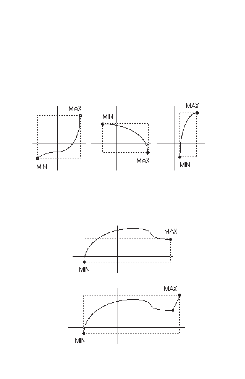
1) The nonlinear function must be totally enclosed by the rectangular area

defined by the minimum an maximum points. Figure 10 gives examples of
the “rectangular area”.

Figure 10. Example of "Rectangular Area".

Figure 11 illustrates a function that is not possible since a portion of the curve
lies outside of the rectangle. In most cases this limitation may be overcome
by simply re-arranging the curve so that the rectangular area is larger. Figure
12 shows the same curve as Figure 11, but slightly modified to allow it to be
programmed into the D2000.

Figure 11. Illegal Function.

Figure 12 Modified Function.

Nonlinear Programming (5-2)

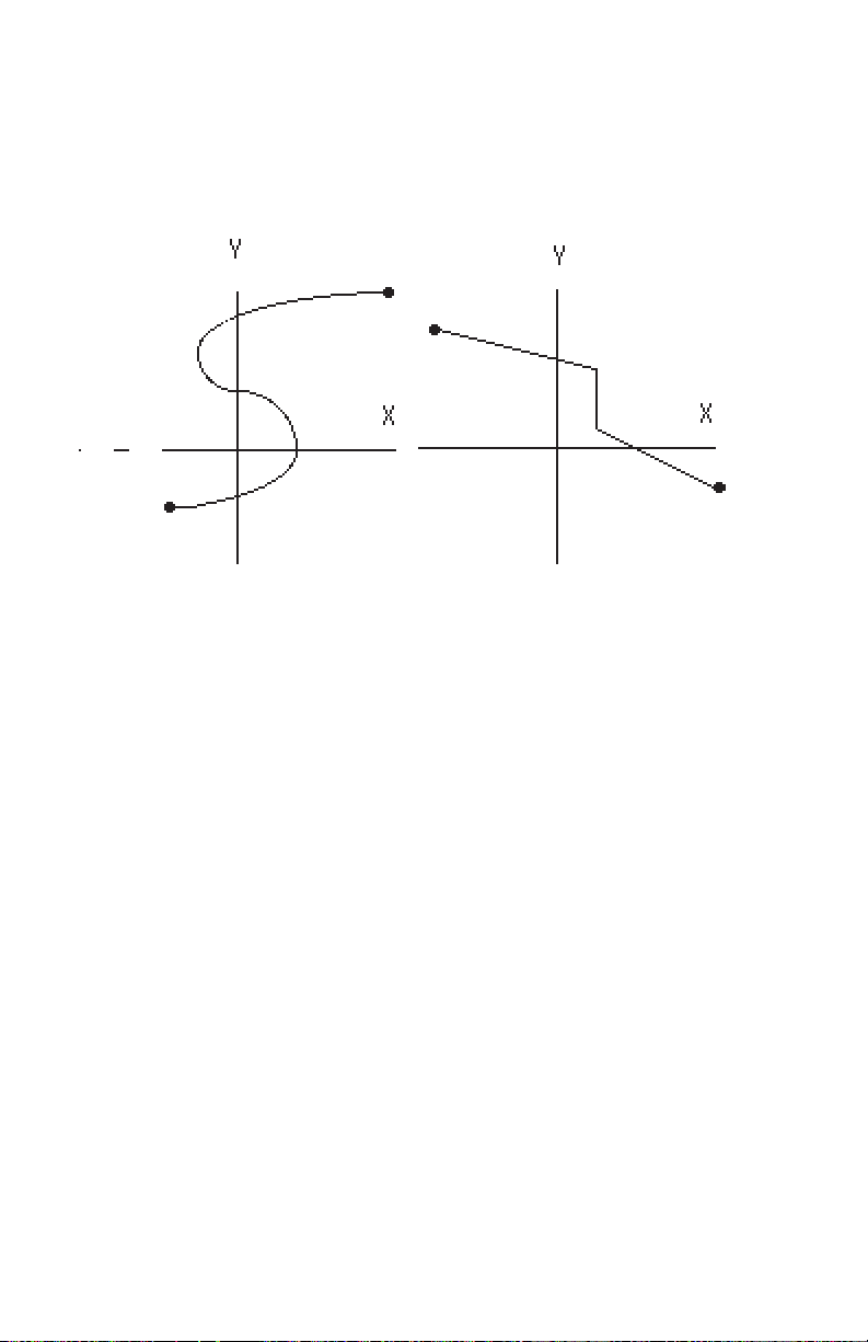
2) The nonlinear function must be a single-valued function of X. That is, for

each input value, there can exist only one output value. Figure 13 shows two
illegal functions. This limitation is seldom encountered in natural phenome­non.

Figure 13. Examples of Illegal Functions.

Programming Steps

1) Define the function data points to be programmed

2) Erase breakpoints

3) Clear zero

4) Use SetUp (SU) command to set number of displayed digits

5) Program the minimum endpoint

6) Program the maximum endpoint

7) Program breakpoints

8) Verify the function

Step 1. Define the function data points to be programmed. The ability of the
D2000 to simulate a nonlinear transfer function is highly dependent on the
location of the breakpoints selected by the programmer. The ultimate
conformity to the desired function is directly dependent on the linear­segment approximation loaded into the module. The D2000 gives the
programmer a great deal of flexibility in how the breakpoints are placed. In
areas where the function curves sharply, or where greater accuracy is
desired, breakpoints may be placed close together for better conformity to
the desired function. The chart in Figure 4 is a handy form to help organize
the breakpoint data.

Nonlinear Programming (5-3)

Step 2. The existing breakpoint table should be cleared by using the Erase
Breakpoints (EB) command. This command will completely erase the
breakpoint table. Any previous breakpoint information will be permanently
lost.

Command: $1WE
Response : *

Command: $1EB
Response: *

Step 3. Clear any data stored in the output offset register by using the Clear
Zero (CZ) command:

Command: $1WE
Response: *

Command: $1CZ
Response: *

Step 4. Use the SetUp (SU) command to program the correct number of
displayed digits:

Command: $1WE
Response: *

Command: $1SU31070182 (typical)
Response: *

Step 5. Start the function programming by setting the minimum point using
the MiNimum (MN) command as described in the linear scaling section.

Step 6. Set the maximum function point with the MaXimum command as
described in the linear scaling section.

Step 7. Use the BreakPoint (BP) command to program the nonlinear
function into memory. Apply the proper excitation to the module for Break­point 00. Use the BreakPoint command to enter the data into memory:

Command: $1WE
Response: *

Command: $1BP00+00100.00
Response: *

Nonlinear Programming (5-4)

It may be useful to verify that the breakpoint data has indeed been recorded
in memory. Without changing the excitation, read the output data:

Command: $1
Response: *+00100.00

The output data should match the data programmed with the Breakpoint
command.

Once Breakpoint 00 has been entered, proceed to Breakpoint 01. Set the
analog excitation for the correct value for Breakpoint 01. Load the breakpoint
into memory using the BreakPoint command. Be sure to specify ‘01’ in the
BreakPoint command:

Command: $1WE
Response: *

Command: $1BP01+00200.00
Response: *

Verify that the data has been entered properly:

Command: $1
Response: +00200.00

Continue this process until all breakpoints have been programmed.
Step 8. Test the input-output transfer function of the module to verify that the

breakpoint data has been entered properly. Large errors in the output data
are generally caused by improper breakpoint programming. In most cases
it is not necessary to repeat the whole breakpoint sequence if the error is
confined to one portion of the curve. Breakpoints may be re-programmed
individually to correct any errors. However, it is not possible to insert new
breakpoints in between existing points of the table to correct for a poor initial
function approximation.

Example N–1

A voltage-output pressure sensor produces 0V @ 100 psi and 5V @ 600 psi.
Its output characteristic is nonlinear and may be described by the equation:

P = 100 + 80 V + 4 V

2

where
V = sensor output in volts

P = pressure in psi
A simple linear equation may be derived by using the endpoint data:

P = 100 + 100V

Nonlinear Programming (5-5)

Unfortunately, describing the sensor output with this equation results in a 25
psi error at V = 2.5V.

To obtain better accuracy, we may approximate the quadratic transfer
function using breakpoints. Since the sensor output range is 0–5V, the
D2131 with an input range of ±5V is most suitable for this application. For
simplicity, we will use only four evenly-spaced breakpoints to plot the
function. This will result in a function approximation with a maximum error
of 1 psi. For better conformity, more breakpoints may be used.

1. First, construct the function table:

Analog Input Output

Minimum 0V +00100.00
Maximum 5V +00600.00
Breakpoint 00 1V +00184.00
Breakpoint 01 2V +00276.00
Breakpoint 02 3V +00376.00
Breakpoint 03 4V +00484.00

Notice that we’ve broken up the curve into five evenly-spaced voltage
segments by using four breakpoints. The breakpoint output values were
obtained by plugging the breakpoint voltage values into the quadratic
equation that describes the sensor.

2. Prepare the D2131 by erasing any stored breakpoints: (All programming

commands must be preceded by a Write Enable (WE) command. In the
interest of simplicity, the Write Enable commands are not shown in this or
any of the following examples.)

Command: $1EB
Response: *

3) Clear any data in the output offset register:

Command: $1CZ
Response: *

4) We will setup the output data to display psi with .1 resolution:

Command: $1SU31070182 (typical)
Response: *

(The SU data may vary depending on your particular module setup. See the
Setup section in the D1000 manual.)

Nonlinear Programming (5-6)

5. Apply 0 volts (short) to the input of the D2131 to enter the minimum point

of 100 psi:

Command: $1MN+00100.00
Response: *

6. To set the maximum point, apply 5V to the input and program the

maximum point to be 600 psi:

Command: $1MX+00600.00
Response: *

7. Program the first breakpoint:

Apply 1 volt to the input and perform the BreakPoint command:

Command: $1BP00+00184.00
Response: *

Verify the breakpoint data:

Command: $1
Response: *+00184.00

Repeat the procedure for the remaining breakpoints:
Apply 2 volts to the input:

Command: $1BP01+00276.00
Response: *

Command: $1
Response: *+00276.00

Apply 3 volts to the input:

Command: $1BP02+00376.00
Response: *

Command: $1
Response: *+00376.00

Apply 4 volts to the input:

Command: $1BP03+00484.00
Response: *

Command: $1
Response: *+00484.00

The function programming is now complete.

Nonlinear Programming (5-7)

8. The transfer function may be verified by applying test inputs to the module

and obtaining output data. The data can then be compared to the original
quadratic equation to check for conformity error.

Example:
Apply .5 volts to the D2131 input and read data:

Command: $1
Response: *+00142.00

To check, plug .5 volts into the quadratic equation:
P = 100 + 80 (.5) + 4 (.5)2 = 141
The conformity error at this point is +1 psi.

Example N–2

A pressure sensor rated for 0-200 psi has a nonlinear transfer function
described by the relationship:

V = 4 x 10-3 P + 5 x 10-6 P

2

V = 0 to 1 volts
P = 0 to 200 psi

Use a D2121 ±1V input module to linearize the sensor output and convert
the data to engineering units.

This example differs from Example N–1 because the desired output data in
psi is the independent variable in the equation. One solution to this problem
would be to convert the equation to a form of P = f (V) and then proceed as
we did in Example N–1. However, this kind of mathematical rigor is not
necessary. To program the D2121, we simply need to construct a table of
X,Y pairs. In this case, we may choose breakpoints to be in even intervals
of psi, and then calculate the matching values of V. Our table with four
breakpoints would look like this:

Input Output

Minimum 0V +00000.00
Maximum +1V +00200.00
Breakpoint 00 .168V +00040.00
Breakpoint 01 .352V +00080.00
Breakpoint 02 .552V +00120.00
Breakpoint 03 .768V +00160.00

Notice that in this case, the breakpoints were selected by picking even
intervals of pressure. The pressure values are then plugged into the sensor

Nonlinear Programming (5-8)

equation to produce the breakpoint voltages. The mechanics of entering the
breakpoints is the same as in Example 1.

If better conformity is required, more breakpoints may be used. However,
breakpoints cannot be simply added to the table at random. Breakpoints
must be entered in sequence starting at the minimum value and progress in
ever-increasing values of the X variable. To obtain better conformity, a new
function table must be started from the beginning. Therefore, to avoid
needless trial and error, it is best to test the breakpoint table on paper to
determine if the conformity error is acceptable. Another approach is to
simply use all 23 breakpoints available for the best conformity.

For this example, we may improve the conformity error by using nine
breakpoints:

Input Output
Minimum 0V +00000.00
Maximum 1V +00200.00
Breakpoint 00 .082V +00020.00
Breakpoint 01 .168V +00040.00
Breakpoint 02 .258V +00060.00
Breakpoint 03 .352V +00080.00
Breakpoint 04 .450V +00100.00
Breakpoint 05 .552V +00120.00
Breakpoint 06 .658V +00140.00
Breakpoint 07 .768V +00160.00
Breakpoint 08 .882V +00180.00

Example N–3

In many cases, the system transfer function may not be known. In these
situations, a D2000 may be programmed empirically using test inputs
derived by the system itself.

A standpipe in a municipal water system has an irregular shape, as shown
in Figure 14. It is desirable to obtain a direct reading of the volume of water
contained in the standpipe. Because of the shape, a simple water height
measurement would give grossly inaccurate readings of volume. Also, the
actual relationship of volume to height is complex and unknown.

The standpipe is 50 feet tall and has a known capacity of 30,000 gallons. A
pressure sensor may be used at the base of the standpipe to obtain a
reading of the water height. Since 1 foot of water produces a pressure of
.4335 psi, the maximum pressure expected is 50 X .4335 = 21.7 psi. The
pressure sensor we will use produces 0–5 volts for pressures of 0–25 psi.
A D2131 ±5V input module will be used as the interface.

Nonlinear Programming (5-9)

Figure 14. Scaling When Transfer Function is Unknown.

Install the pressure sensor and the D2131 in place at the standpipe. Prepare
the D2131 by erasing breakpoints and clearing zero as detailed in Example
N–1. In this case we will setup the D2131 to display four digits which will
result in an output resolution of 10 gallons.

Start programming with the standpipe empty. Enter the minimum value:

Command: $1MN+00000.00
Response: *

In this example, the maximum point may be programmed by filling the

standpipe to obtain the maximum pressure output. However, this is awk­ward and unnecessary. Since the standpipe capacity is known to be 30,000
gallons and the pressure can never reach 25 psi, we can simulate a
maximum that we know can never be attained. To do this we may apply 5V
to the module input to simulate 25 psi. The 5V source does not have to be
accurate. We can set the maximum value to 35,000 gallons, which is more
than the standpipe can hold.

Disconnect the pressure sensor and apply 5V to the module input:

Command: $1MX+35000.00
Response: *

Re-connect the pressure sensor to the D2131. Starting with the standpipe
empty, we may begin to program the breakpoints. We will set a breakpoint
every 1500 gallons for a total of 20 breakpoints.

Nonlinear Programming (5-10)

To set the first breakpoint, fill the standpipe with 1500 gallons of water. Since
we will be using actual volumes of water to ‘calibrate’ the standpipe, the
accuracy at which we can measure 1500 gallons will greatly influence the
final performance of the system.

With 1500 gallons in the standpipe used as the input excitation, program the
first breakpoint:

Command: $1BP00+01500.00
Response: *

Test:

Command: $1
Response: *+01500.00

Fill the standpipe with an additional 1500 gallons to program the second
breakpoint. The standpipe now holds 3000 gallons:

Command: $1BP01+03000.00
Response: *

Command: $1
Response: *+03000.00

Repeat these steps until the standpipe is full. For each step, fill the standpipe
with an additional 1500 gallons and program the breakpoint with the
accumulated amount of water in the standpipe. When the breakpoint
programming is complete, the D2131 will give a very accurate indication of
the volume of water in the standpipe directly in units of gallons.

In this example, the actual transfer function of the system is unknown.
Instead, the function is plotted in the field by applying known inputs to the
system. Note that the voltage produced by the pressure sensor does not
have to be known to program the D2131. However it is wise to record the
voltages produced by the sensor at each breakpoint. With this information,
replacement D2131’s may be programmed with a voltage source to avoid
repeating the tank filling exercise.

Example N–4

Program a D2141 ±10V input module to calculate the square root of the input
signal from 0 to 10V. We’ll keep the units in terms of millivolts so that the
square root of 10,000 millivolts (10V) is 100. To simplify this example, we
will create a function with nine breakpoints at even 1V intervals.

1. Construct the function table:
Analog input Data Output

Minimum 0V +00000.00
Maximum 10V +00100.00
Breakpoint 00 1V +00031.62
Breakpoint 01 2V +00044.72
Breakpoint 02 3V +00054.77
Breakpoint 03 4V +00063.25
Breakpoint 04 5V +00070.71
Breakpoint 05 6V +00077.46
Breakpoint 06 7V +00083.67
Breakpoint 07 8V +00089.44
Breakpoint 08 9V +00094.87

2. Erase breakpoints:

Command: $1EB
Response: *

3. Clear zero:

Command: $1CZ
Response: *

4. Display all digits:

Nonlinear Programming (5-11)

Command: $1SU310701C2 (typical)
Response: *

5. Program minimum by applying 0V (short) to input:

Command: $1MN+00000.00
Response: *

6. Program maximum by applying exactly 10 volts to the input:

Command: $1MX+00100.00
Response: *

7. Program breakpoints:

Apply 1 volt to the input:

Command: $1BP00+00031.62
Response: *

Nonlinear Programming (5-12)

Apply 2 volts to the input:

Command: $1BP01+00044.72
Response: *

Continue until all breakpoints are programmed.

8. Verify the transfer function.

To get better conformity more breakpoints may be programmed, especially
near the minimum end of the scale where the function curvature is greatest.
There is no particular requirement to have breakpoints at regular intervals.
The breakpoint intervals may be varied to achieve the best overall confor­mity. Small breakpoint intervals assure better conformity in areas where the
function curvature is the greatest.

Example N–5

Breakpoints may be used to improve the linearity of a module in linear output
applications.

The D2141 module programmed in Example N–4 is to be programmed back
to its original ±10V input-output transfer function.

1. Define function data:
Analog Input Data Output

Minimum – 10V –10000.00
Maximum +10V +10000.00

(No Breakpoints)

2. Erase breakpoints.

3. Clear zero

4. Setup the displayed output for five digits:

Command: $1SU31070142 (typical)
Response: *

5. Program minimum by applying exactly – 10V to the input:

Command: $1MN–10000.00
Response: *

6. Program maximum by applying +10V to the input:

Command: $1MX+10000.00
Response: *

7. There are no breakpoints to be programmed.

Nonlinear Programming (5-13)

Analog Input Data Output
– 5V –05010.00

0V –00020.00
+ 5V +04990.00

During the verification process, we find that the module exhibits some errors.
This is due to the .1% typical error inherent in the analog-to -digital converter.
The nonlinearity may be corrected by using breakpoints. In this case,
instead of using the breakpoints to create a nonlinear function, they will be
used to ‘straighten’ the nonlinearity of the ADC. Only a few breakpoints are
necessary to reduce the linearity error to .02 % or less. In this case we will
use three breakpoints to linearize the module:

Analog Input Data Output

Minimum – 10V –10000.00
Maximum + 10V +10000.00
Breakpoint 00 – 5V –05000.00
Breakpoint 01 0V +00000.00
Breakpoint 02 +5V +05000.00

Since the minimum and maximum data have already been programmed,
only Step 7 is necessary to program in the breakpoints.

After the breakpoints have been entered, verify the module transfer function:

Analog Input Data Output
– 7.5V –07502.00

0V +00000.00
+7.5V +07498.00

This time the module output is in error by .02 % or less due to linearizing
effect of the breakpoints.

Example N–6

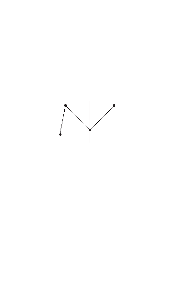
Figure 15. Absolute Value Function.

Nonlinear Programming (5-14)

A D2141 module may be programmed to create an absolute-value function
as shown in Figure 15. However, this function violates the ‘rectangular area’
rule. To overcome this limitation, the function may be re-drawn as shown in
Figure 16. This curve satisfies the ‘rectangular area’ rule. The function table
for this curve looks like this:

Analog Input Data Output

Minimum - 10V -00010.00
Maximum +10V +10000.00
Breakpoint 00 -9.990V +09990.00
Breakpoint 01 0V +00000.00

Figure 16. Modified Absolute Value Function.

The absolute-value function will be valid for inputs between - 9.990V and +
10V. This technique may be used for other functions that violate the
‘rectangular area’ rule.

WARRANTY/DISCLAIMER

OMEGA ENGINEERING, INC. warrants this unit to be free of defects in materials and
workmanship for a period of 13 months from date of purchase. OMEGA’s WARRANTY adds an
additional one (1) month grace period to the normal one (1) year product warranty to cover
handling and shipping time. This ensures that OMEGA’s customers receive maximum
coverage on each product.

If the unit malfunctions, it must be returned to the factory for evaluation. OMEGA’s Customer
Service Department will issue an Authorized Return (AR) number immediately upon phone or
written request. Upon examination by OMEGA, if the unit is found to be defective, it will be
repaired or replaced at no charge. OMEGA’s WARRANTY does not apply to defects resulting
from any action of the purchaser, including but not limited to mishandling, improper interfacing,
operation outside of design limits, improper repair, or unauthorized modification. This
WARRANTY is VOID if the unit shows evidence of having been tampered with or shows evidence
of having been damaged as a result of excessive corrosion; or current, heat, moisture or vibra­tion; improper specification; misapplication; misuse or other operating conditions outside of
OMEGA’s control. Components in which wear is not warranted, include but are not limited to
contact points, fuses, and triacs.

OMEGA is pleased to offer suggestions on the use of its various products. However,
OMEGA neither assumes responsibility for any omissions or errors nor assumes liability
for any damages that result from the use of its products in accordance with information
provided by OMEGA, either verbal or written. OMEGA warrants only that the parts
manufactured by the company will be as specified and free of defects. OMEGA MAKES
NO OTHER WARRANTIES OR REPRESENTATIONS OF ANY KIND WHATSOEVER,
EXPRESSED OR IMPLIED, EXCEPT THAT OF TITLE, AND ALL IMPLIED WARRANTIES
INCLUDING ANY WARRANTY OF MERCHANTABILITY AND FITNESS FOR A PARTICULAR
PURPOSE ARE HEREBY DISCLAIMED. LIMITATION OF LIABILITY: The remedies of pur­chaser set forth herein are exclusive, and the total liability of OMEGA with respect to this
order, whether based on contract, warranty, negligence, indemnification, strict liability or
otherwise, shall not exceed the purchase price of the component upon which liability is
based. In no event shall OMEGA be liable for consequential, incidental or special damages.

CONDITIONS: Equipment sold by OMEGA is not intended to be used, nor shall it be used: (1) as
a “Basic Component” under 10 CFR 21 (NRC), used in or with any nuclear installation or activity;
or (2) in medical applications or used on humans. Should any Product(s) be used in or with any
nuclear installation or activity, medical application, used on humans, or misused in any way,
OMEGA assumes no responsibility as set forth in our basic WARRANTY/ DISCLAIMER language,
and, additionally, purchaser will indemnify OMEGA and hold OMEGA harmless from any liability
or damage whatsoever arising out of the use of the Product(s) in such a manner.

RETURN REQUESTS/INQUIRIES

Direct all warranty and repair requests/inquiries to the OMEGA Customer Service Department.
BEFORE RETURNING ANY PRODUCT(S) TO OMEGA, PURCHASER MUST OBTAIN AN
AUTHORIZED RETURN (AR) NUMBER FROM OMEGA’S CUSTOMER SERVICE DEPARTMENT
(IN ORDER TO AVOID PROCESSING DELAYS). The assigned AR number should then be
marked on the outside of the return package and on any correspondence.

The purchaser is responsible for shipping charges, freight, insurance and proper packaging to
prevent breakage in transit.

FOR WARRANTY

RETURNS, please have
the following information available BEFORE
contacting OMEGA:

1. Purchase Order number under which

the product was PURCHASED,

2. Model and serial number of the product

under warranty, and

3. Repair instructions and/or specific

problems relative to the product.

FOR NON-WARRANTY REPAIRS,

consult
OMEGA for current repair charges. Have the
following information available BEFORE
contacting OMEGA:

1. Purchase Order number to cover the

COST of the repair,

2. Model and serial number of the

product, and

3. Repair instructions and/or specific problems

relative to the product.

OMEGA’s policy is to make running changes, not model changes, whenever an improvement is possible.
This affords our customers the latest in technology and engineering.

OMEGA is a registered trademark of OMEGA ENGINEERING, INC.
© Copyright 2005 OMEGA ENGINEERING, INC. All rights reserved. This document may not be copied, photocopied,

reproduced, translated, or reduced to any electronic medium or machine-readable form, in whole or in part, without
the prior written consent of OMEGA ENGINEERING, INC.

Where Do I Find Everything I Need for

Process Measurement and Control?

OMEGA…Of Course!

Shop online at omega.com

TEMPERATURE

䡺⻬

Thermocouple, RTD & Thermistor Probes, Connectors, Panels & Assemblies

䡺⻬

Wire: Thermocouple, RTD & Thermistor

䡺⻬

Calibrators & Ice Point References

䡺⻬

Recorders, Controllers & Process Monitors

䡺⻬

Infrared Pyrometers

PRESSURE, STRAIN AND FORCE

䡺⻬

Transducers & Strain Gages

䡺⻬

Load Cells & Pressure Gages

䡺⻬

Displacement Transducers

䡺⻬

Instrumentation & Accessories

FLOW/LEVEL

䡺⻬

Rotameters, Gas Mass Flowmeters & Flow Computers

䡺⻬

Air Velocity Indicators

䡺⻬

Turbine/Paddlewheel Systems

䡺⻬

Totalizers & Batch Controllers

pH/CONDUCTIVITY

䡺⻬

pH Electrodes, Testers & Accessories

䡺⻬

Benchtop/Laboratory Meters

䡺⻬

Controllers, Calibrators, Simulators & Pumps

䡺⻬

Industrial pH & Conductivity Equipment

DATA ACQUISITION

䡺⻬

Data Acquisition & Engineering Software

䡺⻬

Communications-Based Acquisition Systems

䡺⻬

Plug-in Cards for Apple, IBM & Compatibles

䡺⻬

Datalogging Systems

䡺⻬

Recorders, Printers & Plotters

HEATERS

䡺⻬

Heating Cable

䡺⻬

Cartridge & Strip Heaters

䡺⻬

Immersion & Band Heaters

䡺⻬

Flexible Heaters

䡺⻬

Laboratory Heaters

ENVIRONMENTAL
MONITORING AND CONTROL

䡺⻬

Metering & Control Instrumentation

䡺⻬

Refractometers

䡺⻬

Pumps & Tubing

䡺⻬

Air, Soil & Water Monitors

䡺⻬

Industrial Water & Wastewater Treatment

䡺⻬

pH, Conductivity & Dissolved Oxygen Instruments

M0661/0605