

Page 1
OCULUS
Pentacam
®
Pentacam® HR
INTERPRETATION GUIDE
3rd edition
Page 2

Foreword
We thank you for the trust you have put in us by purchasing this OCULUS instrument. In
doing so you have chosen a modern, sophisticated product which was manufactured and
tested according to strict quality standards.
Our company has been doing business for over 120 years. Today OCULUS is a mediumsized company focused entirely on developing and manufacturing advanced and innovative
instruments for examinations and surgery on the eye to help ophthalmologists, optometrists
and opticians in their routine work.
The Pentacam® is based on the Scheimpug principle, which generates precise and sharp
images of the anterior eye segment. This instrument takes extremely accurate measurements
and is easy to use.
If you have questions or desire further informations on this product, please turn to your
OCULUS representative or directly to OCULUS.
We will be glad to help you.
OCULUS Optikgeräte GmbH
Note
OCULUS Optikgeräte GmbH wishes to emphasize that the user bears full responsibility
for the correctness of data measured, calculated or displayed using the Pentacam®. The
manufacturer will not accept claims based on erroneous data or misinterpretation. This
Interpretation Guide can no more than assist in the interpretation of examination data
generated by the Pentacam®.
In making a diagnosis physicians should not neglect to consider other medical information
which may be obtainable through other methods such as slit lamp examination or ultrasound
biomicroscopy, judiciously weighing the signicance of each.
This Interpretation Guide should be seen as a complement to the User Guide and Instruction
Manual. The current version of these documents and the Interpretation Guide are on every
Pentacam® Software USB drive and should be read by all users prior to use.
OCULUS has been certified according to DIN EN ISO 13485 and therefore sets high quality
standards in the development, production, quality assurance and servicing of its entire
product range.
Page 3

Table of contents
Table of contents
1 Introduction....................................................................................................................................................5
2 Description of the unit and general remarks..........................................................................................5
3 Differences between the various topography maps of Pentacam®.............................................6-11
3.1 Calculation of corneal power..........................................................................................................................6
3.2 Sagittal power map (also called axial power map)...................................................................................7
3.3 Refractive power map.......................................................................................................................................8
3.4 True Net Power....................................................................................................................................................9
3.5 Equivalent Keratometer Readings power map.........................................................................................10
3.6 Total Cornea Refractive Power map............................................................................................................11
4 Recommended settings and color maps, displays and values....................................................12-14
4.1 Recommended settings...................................................................................................................................12
4.2 Recommended color maps, displays and values......................................................................................13
4.2.1 Screening for corneal refractive surgery.......................................................................................13
4.2.2 Pre-op screening for iris fixated phakic IOL implantation.......................................................13
4.2.3 Glaucoma screening............................................................................................................................14
4.2.4 Cataract surgery and IOL calculation for virgin and post refractive corneas....................14
5 Differences between Placido and elevation-derived curvature maps
by Prof. Michael W. Belin....................................................................................................................15-19
5.1 Keratoconus in OD and OS?..................................................................................................................... .....15
5.2 Form fruste keratoconus?.......................................................................................................................... ....18
6 Fast Screening Report as a first step in examining a patient and evaluating
one’s findings by Ina Conrad-Hengerer, MD................................................................................. 20-27
6.1 Case 1: Unilateral high astigmatism with suspicion of bilateral keratoconus...............................20
6.2 Case 2: Fuchs’ dystrophy with DMEK cataract surgery – progress evaluation...............................23
6.3 Case 3: Corneal injury sustained from an eye drop bottle after cataract surgery.........................26
7 Refractive Power Distribution display by Ina Conrad-Hengerer, MD.......................................28-30
7.1 Visual acuity impairment during nighttime driving with distance spectacles –
nocturnal myopia? ........................................................................................................................................... 28
8 Corneal ectasia.....................................................................................................................................31-35
8.1 Case 1: Ectasia after radial keratotomy by Prof. Renato Ambrósio Jr .............................................31
8.2 Case 2: Ectasia after LASIK? by Prof. Michael W. Belin.........................................................................33
9 Glaucoma...............................................................................................................................................36-46
9.1 Case 1: General screening by Tobias H. Neuhann, MD..........................................................................36
9.2 Case 2: YAG laser iridectomy by Eduardo Viteri, MD.............................................................................37
9.3 Screening for narrow angles by Dilraj S. Grewal, MD...........................................................................39
9.3.1 Case 1.....................................................................................................................................................39
9.3.2 Case 2.....................................................................................................................................................42
9.4 Evaluating the anterior segment in phacomorphic glaucoma by Dilraj S. Grewal, MD..................45
1
Page 4

Table of contents
10 Screening for refractive surgery by Prof. Michael W. Belin................................................47-63
10.1 Screening parameters, 4 Maps Refractive display......................................................................47
10.1.1 Suggested installation settings ...........................................................................................47
10.1.2 Proposed screening parameters ...........................................................................................48
10.1.3 Strategy on how to go through the exams ......................................................................49
10.2 Normal, astigmatic cornea ................................................................................................................49
10.3 Astigmatism on the posterior cornea .............................................................................................52
10.4 Spherical cornea...................................................................................................................................53
10.5 Thin spherical cornea ..........................................................................................................................54
10.6 Thin cornea ............................................................................................................................................55
10.7 Borderline case of keratoconus ........................................................................................................56
10.8 Displaced apex...................................................................................................................................... 57
10.9 Pellucid marginal degeneration .......................................................................................................58
10.10 Asymmetric keratoconus ....................................................................................................................59
10.11 Keratoconus with false negative findings on curvature map ..................................................61
10.12 Keratoconus greater in OD than OS ................................................................................................62
10.13 Classic keratoconus .............................................................................................................................63
11 Corneal Thickness Spatial Profile by Prof. Renato Ambrósio Jr .......................................64-79
11.1 Screening for ectasia by Prof. Renato Ambrósio Jr, Marcela Q. Salomão, MD...................67
11.2 Case 1: Fuchs’ dystrophy by Prof. Renato Ambrósio Jr, Marcela Q. Salomão, MD............72
11.3 Case 2: Ocular hypertension by Prof. Renato Ambrósio Jr,
Marcela Q. Salomão, MD................................................................................................................... 74
11.4 Case 3: Early Fuchs’ dystrophy with glaucoma by Prof. Renato Ambrósio Jr,
Marcela Q. Salomão, MD................................................................................................................... 76
11.5 Screening parameters by Prof. Renato Ambrósio Jr ..................................................................79
12 Belin/Ambrósio Enhanced Ectasia Display.............................................................................80-102
12.1 Why elevation is displayed by Prof. Michael W. Belin ...............................................................80
12.2 Simplifying preoperative keratoconus screening by Prof. Michael W. Belin,
Prof. Renato Ambrósio Jr, Andreas Steinmüller, MSc................................................................88
12.3 Interpretation of the Belin/Ambrósio Enhanced Ectasia Display............................................94
12.4 Pachymetry evaluation........................................................................................................................96
12.5 Ectasia susceptibility revealed by the Belin/Ambrósio Enhanced Ectasia Display.............96
12.6 Early ectasia with asymmetric keratoconus by Prof. Renato Ambrósio Jr,
Fernando Faria- Correia, MD, Allan Luz, MD...............................................................................100
13 Locating the cone by Prof. Michael W. Belin..............................................................................102
14 The corneal densitometry screen, Sorcha S. Ní Dhubhghaill, MB, PhD,
Jos J. Rozema, MSc, PhD......................................................................................................... 103-107
14.1 Keratic precipitates............................................................................................................................104
14.2 Position and depth of INTACS® rings............................................................................................106
14.3 DSAEK with specks at the interface..............................................................................................107
15 Using Pentacam® technology to evaluate corneal scars, planning and documenting
surgery outcomes by Arun C. Gulani, MD, MS.................................................................. 108-116
15.1 Case 1: Corneal scar with RK incisions and cataract...............................................................112
15.2 Case 2: Keratoconus with congenital cataract, high myopia and high astigmatism.....115
2
Page 5

Table of contents
16 INTACS® implantation...............................................................................................................117-122
16.1 Case 1: by Prof. Michael W. Belin....................................................................................................117
16.2 Case 2: INTACS® after PRK by Alain-Nicolas Gilg, MD............................................................ 119
16.3 Case 3: INTACS® & crosslinking by Prof. Renato Ambrósio Jr,
Fernando Faria-Correia, MD, Allan Luz, MD ................................................................................ 121
17 Holladay Report & Holladay EKR65 Detail Report by Jack T. Holladay, MD................123-136
17.1 Holladay Report....................................................................................................................................123
17.2 Holladay EKR65 Detail Report.........................................................................................................129
17.3 Case 1: Holladay Report & Holladay EKR65 Detail Report of a normal exam ..................130
17.4 Case 2: Holladay Report & Holladay EKR65 Detail Report of a keratoconus exam.........133
17.5 Case 3: Holladay Report & Holladay EKR65 Detail Report of a post LASIK exam............135
18 Corneal tomographic analysis is essential before cataract surgery -
4 steps in screening candidates for premium IOLs by Prof. Naoyuki Maeda............. 137-140
18.1 Corneal topography for selecting premium IOLs.......................................................................137
18.2 Step 1: Evaluation of corneal irregular astigmatism.................................................................140
18.3 Step 2: Detection of abnormal corneal shape ............................................................................ 140
18.4 Step 3: Evaluation of corneal spherical aberration ...................................................................140
18.5 Step 4: Evaluation of corneal cylinder ..........................................................................................140
19 Dependency of effective phacoemulsification time on Pentacam® Nucleus Staging (PNS)
by Mehdi Shajari, MD, Wolfgang Mayer, MD, Prof. Thomas Kohnen............................141-142
19.1 Introduction ..........................................................................................................................................141
19.2 Case 1: Low PNS and low EPT .........................................................................................................142
19.3 Case 2: High PNS and high EPT ......................................................................................................142
20 Total corneal astigmatism for toric IOL by Giacomo Savini, MD...................................143-148
20.1 Case 1: Cylinder overcorrection from measurement of keratometric astigmatism
in an eye with WTRA..........................................................................................................................144
20.2 Case 2: Cylinder undercorrection from measurement of keratometric astigmatism
in an eye with ATRA ...........................................................................................................................146
20.3 Case 3: Cylinder overcorrection from measurement of keratometric astigmatism .........147
21 Overview about IOL power calculation formulas for different eye types............................. 149
22 Phakic IOL implantation .........................................................................................................150-160
22.1 Manual pre-op simulation and post-op control by Eduardo Viteri, MD.............................150
22.1.1 Pre-operative evaluation...................................................................................................150
22.1.2 Post-operative evaluation.................................................................................................151
22.2 3D pIOL Simulation Software and Aging Prediction by Prof. Burkhard Dick,
Sabine Buchner, Optometrist............................................................................................................151
22.2.1 Myopic Artisan/Verisyse, 6/8.5 mm ................................................................................151
22.2.2 Toric Artisan/Verisyse, 5/8.5 mm ....................................................................................155
22.3 Patient selection criteria by Prof. Burkhard Dick,
Sabine Buchner, Optometrist............................................................................................................157
22.4 Case example of ectasia after LASIK, crosslinking and pIOL implantation
by Prof. Renato Ambrósio Jr, Fernando Faria-Correia, MD, Allan Luz, MD.........................159
3
Page 6

Table of contents
23 Case reports from daily practice.............................................................................................161-172
23.1 Case 1: Cortical cataract by Tobias H. Neuhann, MD................................................................161
23.2 Case 2: Remove sutures after corneal transplant surgery?
by Tobias H. Neuhann, MD................................................................................................................ 162
23.3 Case 3: Keratoconus and cataract by Tobias H. Neuhann, MD...............................................163
23.4 Case 4: Corneal infiltrate by Prof. Renato Ambrósio Jr ...........................................................166
23.5 Case 5: Incisional edema, by Prof. Renato Ambrósio Jr ...........................................................168
23.6 Case 6: Corneal thinning after herpetic keratitis by Prof. Renato Ambrósio Jr ................169
23.7 Case 7: Epithelial ingrowth after keratomileusis in situ
by Prof. Renato Ambrósio Jr ............................................................................................................. 171
24 Scheimpflug and slit lamp images..........................................................................................173-178
24.1 Corneal dystrophy.................................................................................................................................173
24.2 Congenital anterior pyramid cataract............................................................................................174
24.3 Posterior capsular cataract.................................................................................................................175
24.4 Nuclear cataract....................................................................................................................................176
24.5 Posterior synechia.................................................................................................................................177
24.6 Pterygium................................................................................................................................................178
25 Orthokeratology, general screening by Alain-Nicolas Gilg, MD......................................179-181
26 Important studies and case reports.......................................................................................182-198
26.1 Refractive studies.................................................................................................................................182
26.2 Case reports............................................................................................................................................191
26.3 Cataract studies....................................................................................................................................191
26.4 Case reports...........................................................................................................................................196
26.5 Glaucoma studies.................................................................................................................................196
26.6 Case reports...........................................................................................................................................198
27 References.................................................................................................................................... 199-201
28 List of illustrations......................................................................................................................202-205
29 Tables directory.....................................................................................................................................207
30 List of abbreviations....................................................................................................................208-209
31 Authors and contact addresses................................................................................................210-211
4
Page 7

1 Introduction
2 Description of the unit
and general remarks
1 Introduction
This guide is intended to assist Pentacam®/Pentacam® HR (referred to here as Pentacam®) users in
interpreting the results and screens of the Pentacam®. We may not have covered everything which
might be of interest, and we therefore ask anyone using the Pentacam® for their help in improving
this guide step by step. Please forward us any cases or observations of particular interest, and we
will be happy to incorporate them in this guide.
This guide cannot, of course, replace the knowledge and experiences that only come from long
years of medical studies and professional practice, but it will be of help in cases of doubt as well
as to beginners. At the same time, since medical findings may also depend on the practitioner’s
personal experience and perceptions, the individual patient’s history or the particular combination
of instruments used, it is quite possible for results obtained by other means to differ from those
shown in this guide yet be nonetheless valid.
2 Description of the unit and general
remarks
The OCULUS Pentacam® is a rotating Scheimpflug camera. The rotational measuring procedure
generates Scheimpflug images in three dimensions, with the dot matrix fine-meshed in the centre
due to the rotation. It takes a maximum of 2 seconds to generate a complete image of the anterior
eye segment. Any eye movement is detected by a second camera and corrected for in the process.
The Pentacam® calculates a 3D model of the anterior eye segment from as many as 25.000
(HR: 138.000) distinct elevation points.
The topography and pachymetry of the entire anterior and posterior surface of the cornea from
limbus to limbus are calculated and depicted. The analysis of the anterior eye segment includes a
calculation of the chamber angle, chamber volume and chamber height and a manual measuring
function that can be applied to any location in the anterior chamber of the eye. Images of the
anterior and posterior surface of the cornea, the iris and the anterior and posterior surface of
the lens are generated in a moveable virtual eye. The densitometry of the lens and cornea is
automatically quantified.
The Scheimpflug images taken during the examination are digitalized in the main unit, and all
image data are transferred to the PC.
When the examination is finished, the PC calculates a 3D virtual model of the anterior eye segment,
from which all additional information is derived.
5
Page 8

3 Differences between the various topography maps of Pentacam
®
3 Differences between the various
topography maps of Pentacam
3.1 Calculation of corneal power
Corneal Placido topographers measure geometrical corneal slope values. These values are converted
into curvature values e.g. values of axial (sagittal) curvature or instantaneous (tangential) curvature
which are initially given in mm. The Pentacam® measures geometrical height (elevation) values,
which are likewise converted into values of axial (sagittal) or instantaneous (tangential) curvature
and given in mm. These geometrical radius (mm) values are commonly converted it into refractive
power values, which are given in diopters (D). This is normally done according the simple formula of
D = (1.3375-1)*(1000)/Rmm.
A. The refractive effect
A sphere (sph) has the same radius of curvature at every point of its surface; however, due to
the phenomenon of spherical aberration (SA) its refractive power is not the same everywhere. If
the effect of SA is not taken into account, a corneal sphere with a radius of, say, 7.5 mm may be
considered to have the same refractive power of 45 D at every point of its surface (assuming the
keratometer calibration index of 1.3375, see below). Due to SA, however, the refractive power in the
periphery is actually higher. The Pentacam® refractive maps, as they are called, are calculated on the
basis of “Snell’s law” of refraction using precision ray tracing, thereby taking this effect into account.
®
B. Inclusion of anterior/posterior surface
By convention most keratometers use the refractive index of 1.3375 when calculating the dioptric
power of the anterior radius; in doing so they assume the cornea to have a single refracting
surface. However, it has been known for quite some time that this keratometric index is not the
best approximation to the rather physiological power of the cornea. Due to the contribution of
the posterior surface and the more rather refractive index of the cornea (n cornea = 1.376), the
True Net Power of the cornea, calculated using thick lens models or high-precision ray tracing,
is lower than the value reported by standard keratometry. The deviation between True Net Power
and corneal power as determined by standard keratometry (Sim K’s) becomes even greater when
dealing with corneas after excimer laser ablation (LASIK, LASEK and PRK) of the anterior surface.
After refractive corneal surgery it is no longer possible to calculate corneal refractive power based
only on the anterior surface, as the ratio between the anterior and posterior radius of the cornea
has changed considerably. When the calcultio of the total corneal astigmatism comes into focus the
effect of the posterior corneal surface cannot be disregarded anymore. Depending to the orientation
of the anterior and posterior corneal kertometry the total corneal astigmatism can be over or
underestimated and the axis of the total corneal astigmatism is influenced [1].
6
Page 9

3 Differences between the various topography maps of Pentacam
®
C. The refractive index
For historical reasons, most Placido topographers and keratometers use the refractive index of 1.3375
for calculating corneal refractive power. However, this refractive index is actually incorrect even for
the untreated eye (n ≈ 1.332). It assumes the ratio between the anterior and posterior curvature of
the cornea to be constant. Many intraocular lens (IOL) power calculation formulas use the incorrect
‘K-reading’, necessitating empirical correction to obtain the correct IOL power even in normal cases.
Care should also be taken when using ‘K-readings’ from post-LASIK corneas or based on True Net
Power or ray tracing, as the resultant D readings will be out of range for the applied IOL calculation
formulas unless they are corrected for or converted into equivalent keratometer readings (EKR). Some
modern formulas are able to deal with the rather measured curvatures of the front and back surface
of the cornea, however.
D. Location of the principal planes
Calculation of corneal power by ray tracing involves sending parallel light through the cornea.
It must take into account that each light beam is refracted according to the refractive index
(1.376/1.336), the slope of the surfaces, and the exact location of refraction. This is necessary
because the principal planes of the anterior and posterior surface differ slightly from one another due
tocorneal thickness. The Pentacam® is able to measure the anterior as well as the posterior surface of
the cornea. This allows further corrections to be made. The Pentacam® provides a number of different
maps for predicting corneal power.
3.2 Sagittal power map (also called axial power map)
This is the common Placido style map with corneal power calculated using a refractive index of
1.3375 and the simple formula D = (1.3375-1)*(1000)/Rmm. It shows power values (Figure 1) similar
to those of other Placido topographers.
Figure 1: Sagittal power map of a sphere, r= 8 mm
7
Page 10

3 Differences between the various topography maps of Pentacam
®
3.3 Refractive power map
This map (Figure 3) uses only values from the anterior surface, but it also takes effect “A” (see above)
into account. It calculates corneal power according to Snell’s law of refraction assuming a refractive
index of 1.3375 to convert curvature into refractive power (Figure 2). This is a map that other
Placido topographers also may show because it only considers the anterior surface.
Figure 2: Snell´s law of refraction
Figure 3: Refractive power map of a sphere, r = 8 mm
8
Page 11

3 Differences between the various topography maps of Pentacam
3.4 True Net Power
This map (Figure 4) shows the optical power of the cornea based on two different refractive indices,
one for the anterior (corneal tissue: 1.376) and one for the posterior surface (aqueous humour:
1.336), as well as the sagittal curvature of each. These results are aggregated. The True Net Power
map thus takes effects “A” and "B" into account. The underlying equation is:
®
TrueNet Power =
1,376 -1
r
ant_surface
1000 +
*
1,336 -1,376
r
post_surface
1000
*
Figure 4: True Net Power map calculated by two spheric surfaces of
anterior r = 8 mm and posterior r = 6.58 mm
9
Page 12

3 Differences between the various topography maps of Pentacam
®
3.5 Equivalent Keratometer Readings power map
This map (Figure 5) was designed to take into account the refractive effects of both the anterior
and the posterior surface. Another requirement was that it should output power values which
in normal cases (no Lasik) would be comparable with simulated K (SimK) values, which are
usually derived from sagittal curvature map. Its output is therefore also referred to as Equivalent
Keratometer Readings (EKR). It calculates power according to Snell’s law using the refractive
indices of corneal tissue and aqueous humour and aggregating the values for anterior and posterior
power. Then the output is shifted such that for a normal eye (posterior corneal radius 82% of
anterior corneal radius) its values (EKR) are identical to those of SimK readings from a sagittal map.
In other words, the EKR map is corrected by adding the error that would be created by a refractive
index of 1.3375 in a sagittal map. In this way it provides equivalent K-values (EKR) that can be
used in IOL formulas that correct for n=1.3375. The EKR map thus takes into account effects "A",
"B" and "C".
Figure 5: EKR power map calculated by twospheric surfaces of
anterior r = 8 mm and posterior r = 6.58 mm
The study to validate the method was conducted using the Holladay 2 formula. Here it was determined that after LASIK the best correlation with the traditional method, with a mean prediction
error of -0.06 D ± 0.56 D, is obtained using a mean zonal EKR for the 4.5 mm zone. For post-RK
patients, the mean prediction error is –0.04 D ± 0.94 D [2].
10
Page 13

3 Differences between the various topography maps of Pentacam
3.6 Total Cornea Refractive Power map
This map (Figure 7) uses ray tracing to calculate the refractive power of the cornea. It takes into
account how parallel light beams are refracted according to the relevant refractive indices (1.376
and 1.336), the exact location of refraction and the slope of the surfaces. The location of refraction
is a determinant of surface slope, since the anterior and posterior surfaces have slightly differing
principal planes due to corneal thickness. In this way the map takes effects "A", "B", "C" and
"D" into account. Its results are more realistic than any other, but they will deviate from normal
(sagittal) SimK values so they cannot be used in conventional IOL formulas.
®
Figure 6: Calculation of power according to Snell´s law taking the different refractive
indices and the different principal planes of the anterior and posterior corneal
surfaces into account
Figure 7: Total Corneal Refractive Power map calculated by two spheric surfaces
of anterior r = 8 mm and posterior r = 6.58 mm and pachimetry
11
Page 14

4 Recommended settings and color maps, displays and values
4 Recommended settings and color maps,
displays and values
Physicians who are starting to work with the Pentacam® often turn to us with questions on settings
such as step width on the color scale, or which maps and values to consider before doing LASIK, PRK,
RK or phakic IOL (pIOL) implantation or in keratoconus examinations etc.
In the following chapter we present our recommendations on the more frequently addressed issues.
Hopefully they will also cover most of your questions or even provide new insights as you work
through them. They are no more than recommendations and not necessarily intended to discourage
you from using other maps and settings that you may have found to work best for you.
4.1 Recommended settings
When working through the following chapters it is advisable to consistently use the same settings so
as to be able to reproduce the values given.
In the elevation maps, use a sphere fitted in float (BFS) and set the calculation diameter to
manual and use 8 mm or 9 mm
In the scan menu, select “25 images per scan” and “auto release”
Keratometer presentation: R flat/R steep, unitdiopter (D)
Corneal form factor asphericity Q:
Q < 0: Untreated cornea, normal case
Q > 1: Treated cornea LASIK/PRK/RK etc
Color scale: American style
Step width:
Normal (10 μm) for pachymetry maps
Normal (1 D) for topography maps
Rel. (2.5 μm) Minimum for elevation maps
Use the 9 mm loupe function to obtain maps comparable with those of Placido based
topographers
12
Page 15

4 Recommended settings and color maps, displays and values
4.2 Recommended color maps, displays and values
4.2.1 Screening for corneal refractive surgery
We recommend using the following maps and analysis displays:
Fast Screening Report to check whether the displayed parameters are within normal limits
4 Maps Refractive to check the pachymetry, topography and elevation maps of both corneal
surfaces
Belin/Ambrósio Enhanced Ectasia Display to check whether there deviations from normal limits
which can be a sign of early ectatic changesor keratoconus
Zernike Analysis to see whether the LOA or HOA are withon normal limits
Important values: R flat and R steep, asti and axis, Q-value, QS, pachymetry at thinnest spot and
pupil centers, distance between the corneal apex and thinnest spot. In the elevation maps please
use the parameters recommended in chapter 10.1.2
4.2.2 Pre-op screening for iris fixated phakic IOL implantation
We recommend using the following maps and analysis displays:
The 3D pIOL Simulation Software and Aging Prediction prior to iris fixated pIOL implantation
(available in the Pentacam® HR only). Calculate the required pIOL power using the implanted
calculator. Use the database to find a pIOL that best matches the patient’s subjective refraction.
Its fit in the anterior chamber is simulated in 3D and the minimum clearances are displayed. The
aging simulation allows a simulation of the pIOL position in up to 30 years. Double-check your
calculations and evaluations with the manufacturer of the respective pIOL
For all further pIOL e.g. Intraocular Contact Lens (ICL): Scheimpflug images to obtain information
on the dimensions of the anterior chamber, the iris curve and the densitometry of the cornea and
crystal lens. The view of the anterior chamber angle (ACA) shows whether there is an open or
closed angle
Evaluate the horizontal corneal diameter (HWTW). It is displayed automatically if the new iris
camera optic is built in. If not it can be measured manually in the Scheimpflug image at the 180°
position (horizontal)
Important values: R flat and R steep, asti and axis, HWTW, Q-value, QS, anterior chamber depth
(ACD) pachymetry in the thinnest spot and in the pupil center
13
Page 16

4 Recommended settings and color maps, displays and values
4.2.3 Glaucoma screening
We recommend using the following maps and analysis displays:
Fast Screening Report to check whether the displayed parameters are within normal limits
General Overview display to view the chamber angle in the Scheimpflug images and corneal
thickness. While clicking to the button “Enter IOP” the tonometrically measured IOP can be
entered manually or the respective IOP change can be viewed. The displayed IOP is based on
pre-programmed IOP corrections tables. For more details refer to the Pentacam® User Guide
Important values: ACD, ACV, ACA, Q-value, QS, pachymetry, IOP-correction
4.2.4 Cataract surgery and IOL calculation for virgin and post refractive corneas
We recommend using the following maps and analysis displays
Fast Screening Report to check whether the displayed parameters are within normal limits
Cataract Pre-OP Display that offers a comprehensive overview. Prof. Maeda recommended the
4 following steps to select the IOL:
1. Evaluation of corneal irregularities
2. Corneal shape assessment
3. Evaluations of corneal spherical aberrations
4. Evaluations of the corneal astigmatism
(An article was published in „The Highlights of Ophthalmology“ Assessment of Corneal Optical
Quality for Premium IOLs with Pentacam®“ Highlights of Ophthalmology • Vol. 39, Nº 4, 2011)
Zernike Analysis to determine the amount HOA and LOA
ACD, manual horizontal white-to-white (HWTW) for keratometry readings from virgin eyes
Scheimpflug images to obtain information on the dimensions of the anterior chamber and the
condition of the crystalline lens. Lens density can be quantified in a single location, a line, an area
or a volume, as desired. The grading PNS can be used for optimizing Phaco settings (doi:10.1016/j.
jcrs.2009.08.032) and for the effective phaco time (http://dx.doi.org/10.1016/j.ajo.2013.09.017)
The Holladay Report and the Holladay EKR65 Detail Report for a comprehensive overview of the
cornea. This includes the topographic as well as the pachymetry map and the anterior and
posterior elevation maps. For more information refer to chapter 17
The BESSt formula, developed from Edmondo Borrasio, MD. This requires Rm anterior,
Rm posterior, CCT and ACD doi:10.1016/j.jcrs.2006.08.037
Okulix or Phaco Optics, which are IOL power calculation software based on the ray tracing
principle. More information can be found under: www.phacoptics.com; www.okulix.de
Important values: Keratometry, asti and axis, Q-value, QS, ACD, pachymetry in the thinnest spot
and in the pupil center
14
Page 17

5 Differences between Placido and
elevation-derived curvature maps
5 Differences between Placido and
elevation-derived curvature maps
by Prof. Michael W. Belin
5.1 Keratoconus in OD and OS?
The case shown below explains the difference between suspicious and significant elevation maps
and numbers. The topographic map (Figure 8) shows the left and right eye but gives no unequivocal
statement if it is a keratoconus or not.
Figure 8: Placido based topography of OD and OS allowing no conclusion regarding
keratoconus
The right eye seems to be fine. The left eye is a little steeper. The Pentacam® 4 Maps Selectable
answers clearly the question.
15
Page 18
5 Differences between Placido and
elevation-derived curvature maps
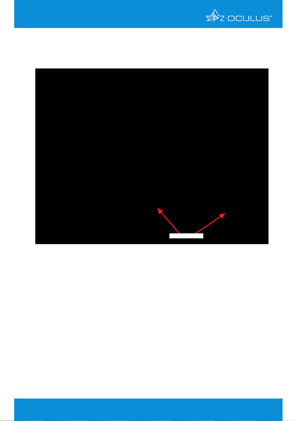
The right eye (Figure 9) has a regular corneal thickness, but the elevation maps of the anterior and
posterior surface indicates this cornea as a suspicious cornea. Both sides show an inferior position
of the cone with suspicious elevations.
suspicious elevation
Figure 9: 4 Maps Selectable showing keratoconus-suspicious elevations in OD
16
Page 19
5 Differences between Placido and
elevation-derived curvature maps
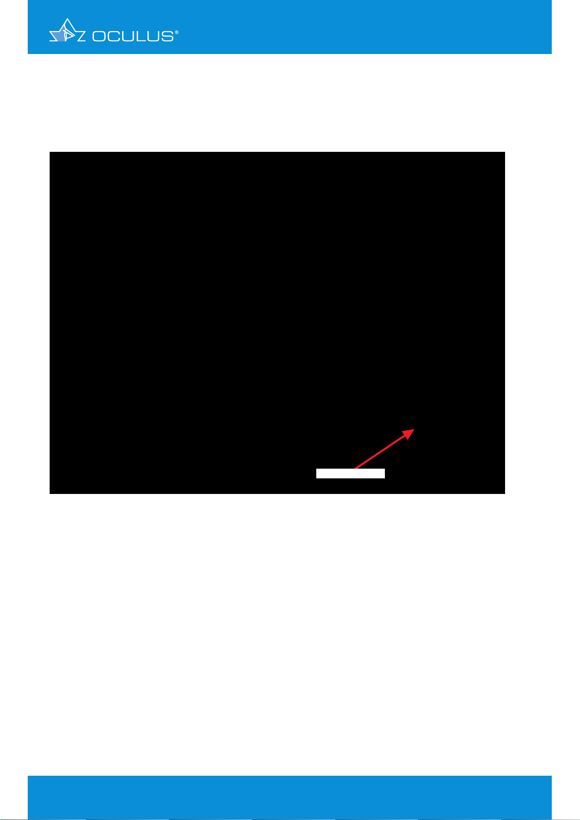
The left eye (Figure 10) indicates an inferior steepening, but a smooth anterior elevation map.
The reason for the thinning in the pachymetry map is the posterior elevation map, where there
are significant elevations of more than 30 μm. Note that the position of the thinning in the
pachymetry map and the highest spot on the elevation map are exactly at the same position.
significant elevation
Figure 10: 4 Maps Selectable showing significant elevation in OS
This is an excellent example to document that topography or anterior elevation only does not
indicate keratoconus.
17
Page 20

5 Differences between Placido and
elevation-derived curvature maps
5.2 Form fruste keratoconus?
A 47-year-old female presented for a second opinion. She had previously been told she was not a
candidate for refractive surgery and that she had “form fruste” keratoconus.
Her exam had revealed a BSCVA 20/20+ OD, and the slit lamp and external examination findings had
been WNL. However, Placido topography showed the following (Figure 11):
Figure 11: Placido based topography of OD and OS
Pentacam® anterior segment analysis revealed normal pachymetry (normal distribution & central
thickness > 650 μm).
The anterior and posterior elevation revealed a slightly decentered apex. This had led to a “false
positive” inferior steepening on the curvature map. Custom LASIK was performed without incident
(Figure 12, Figure 13).
Note:
This case illustrates the limitations of curvature analysis in trying to analyze a shape abnormality.
Curvature is a reference-based measurement and in this case, inaccurately reflects shape
information. Elevation data are independent of axis or orientation and does not have the false
positive rates as curvature maps commonly do.
18
Page 21

5 Differences between Placido and
elevation-derived curvature maps
Figure 12: 4 Maps Selectable showing a form fruste keratoconus false-positive
topography in OS
Figure 13: 4 Maps Selectable showing a form fruste keratoconus false-positive
topography in OD
19
Page 22

6 The Fast Screening Report
6 The Fast Screening Report as a first
step in examining a patient and evaluating
one’s findings
by Ina Conrad-Hengerer, MD
The Fast Screening Report is a very good way of gaining a quick overview when examining patients,
especially when they are presenting for the first time. The Pentacam® analysis is a contactless
examination routine which provides you with all relevant data in a mere two seconds. These are
compared with normative data and converted to index (marker) values using suitable algorithms.
These index values can give helpful indications of possible underlying pathology. How does the
anterior chamber compare with that of a normal eye? Or how about the pachymetry or the elevation
data of the front or back surface of the cornea? Might there be something remarkable about the
patient’s corneal densitometry? The black line always indicates the value of the current patient, and
its position in the grey bar chart shows where it comes to lie in a standard normal distribution. In the
red-and-green chart this normal distribution is shown in green so that it can be compared with that
of the relevant pathological patient group, shown in red. The navigation bar at the top of the Fast
Screening Report leads you to other maps. If a suspicious value has been detected, it will indicate the
name of the map with which this can be explored further. Clicking on the name will take you directly
to the relevant map. In the lower part of the Fast Screening Report you can see whether the corneal
elevation data (BAD D) are within the normal range or not, whether there is keratoconus, and if so, of
what degree (TKC), and if there is a cataract, the degree of nuclear opacity (PNS).
6.1 Case 1: Unilateral high astigmatism with suspicion of bilateral
keratoconus
A male patient aged 45 years presented for the first time in 2010 to have his distance spectacles
refitted. He reported having a long history of amblyopia of his left eye with a visual acuity of 20/100
– 20/67 at best and no known strabismus. Lang’s stereotest I was positive. Correction with sph 0.00
cyl -5.00 A 14° gave him a visual acuity of 20/25 on his left eye, while sph -0.50 cyl -0.50 A 170°
improved his visual acuity to 20/20 on the right.
Slit lamp microscopy showed clear, refracting media bilaterally with no corneal scarring or other
abnormalities. Fundoscopy revealed 2 chorioatrophic foci in the left eye. All other examinations
(without the Pentacam®) yielded unremarkable results.
It was not until 5 years later that the patient presented again, now suspecting that the refraction of
his right eye had changed. The slit lamp microscopy findings were virtually unchanged.
OD: sph -0.50 cyl -1.25 A 167° visual acuity (VA) 20/20
OS: sph 0.00 cyl -4.75 A 14° visual acuity (VA) 20/25
The Pentacam® Fast Screening Report provides an immediate and clear picture of the unusual
pachymetry and elevation profile of the anterior and posterior corneal surface (Figure 14), whereas
the maps appear relatively normal. On following the navigation bar to the Belin/Ambrósio Enhanced
Ectasia Display one finds unmistakable evidence of an advanced keratoconus of both eyes (Figure 16,
Figure 17). Here the Pentacam® reveals a disease that the patient could have been made aware of
many years earlier.
The patient was informed about this corneal pathology and its prognosis. To improve his visual acuity
he had a rigid contact lens fitted for his left eye. He is coming for follow-up every six months to
monitor how the disease progresses.
20
Page 23

6 The Fast Screening Report
Figure 14: Fast Screening Report showing abnormal pachymetry and elevation data with
unambiguous signs of keratoconus in OD
Figure 15: Fast Screening Report showing abnormal pachymetry and elevation data with
unambiguous signs of keratoconus in OS
21
Page 24

6 The Fast Screening Report
Figure 16: Belin/Ambrósio Enhanced Ectasia Display (version III) showing keratokonus in OD
Figure 17: Belin/Ambrósio Enhanced Ectasia Display (version III) showing keratokonus in OS
22
Page 25

6 The Fast Screening Report
6.2 Case 2: Fuchs’ dystrophy with DMEK cataract surgery –
progress evaluation
A 63-year-old female patient with bilateral cataract and Fuchs’ dystrophy underwent combined
cataract and DMEK surgery. This section reports on her progress, documenting the condition of
her right eye prior to surgery with the Fast Screening Report (Figure 19) and the Corneal Optical
Densitometry display (Figure 21). The symptoms of Fuchs’ dystrophy are clearly to be seen in these
displays. After the surgery it was possible to follow her course of healing, marked by gradual
deturgescence of the corneal stroma. From follow-up measurements performed one month after
the surgery (Figure 22) it was verified that the corneal graft lay flat against the host stroma, and
transplant deturgenscence was functionally assessed on the basis of the Compare 4 Exams display
(Figure 18). At one week postoperative central apical corneal thickness measured 670 μm. In the
course of the following 8 days it increased to 704 μm and after another 9 days had dropped back
to 630 μm. At one month postoperative it had reached a relatively normal value of 582 μm. Since
the graft was obviously functioning well, there was no need to force further deturgenscence with
hyperosmolar eye drops. At 4 weeks postoperative her right eye showed refraction values of sph
+0.50 cyl -1.00 A 108° and a visual acuity of 20/25. Her combined cataract and DMEK surgery has
turned out well, as is also confirmed by the Fast Screening Report (Figure 20). She currently comes
regularly every 2 weeks for follow-up.
Figure 18: Compare 4 Exams for postoperative monitoring of corneal deturgescence
over the course of one month
23
Page 26

6 The Fast Screening Report
Figure 19: Fast Screening Report showing the presurgical condition in a case of
Fuchs’ dystrophy
Figure 20: Fast Screening Report at one month after DMEK surgery
24
Page 27

6 The Fast Screening Report
Figure 21: Corneal Optical Densitometry showing the presurgical condition in a case of
Fuchs’ dystrophy
Figure 22: Corneal Optical Densitometry at one month after DMEK surgery
25
Page 28

6 The Fast Screening Report
6.3 Case 3: Corneal injury sustained from an eye drop bottle after
cataract surgery
A 54-year-old patient underwent cataract surgery on his highly myopic right eye. The surgery was
performed without any complications, resulting in a postoperative visual acuity of 20/20 with
refraction values of sph -1.75 cyl -0.75 A 25°. After 3 weeks the patient complained of deteriorated
visual acuity without pain.
Slit lamp microscopy showed the cornea to be completely transparent, with a small irregularity
paracentrally. His refraction had changed to sph -4.50 cyl -1.50 A 108° and his visual acuity had
dropped to 20/25, and there was no intraocular irritation. The possibility of a macular oedema
(Irvine-Glass syndrome) was reliably excluded by fundoscopy. The patient expressed dissatisfaction
at this unexpected turn of events, but on inquiry remembered having knocked the eye drop bottle
against his right eye.
Analysis based on the Pentacam® Fast Screening Report revealed an abnormal value for K Max
(anterior surface) as well as anterior and posterior elevation (Figure 23). After calling up the
4 Maps Refractive color display via the navigation bar it was possible explain the changes to
the patient. He was able to see for himself the abnormal distribution of refractive power and
anterior elevation profile around the centre of his right pupil (Figure 24). A week later Pentacam®
measurements showed that the disturbance had subsided, with refraction values of sph -2.00 cyl
-0.25 A 0° and visual acuity back at 20/20. The patient was shown the Compare 2 Exams display,
demonstrating the improvement that had occurred in only a week (Figure 25). It was decided to
postpone refitting his spectacle lenses by 2 weeks, since the Pentacam® analysis indicated that his
right-eye refraction had not yet reached its ultimate distribution.
Figure 23: Fast Screening Report showing suspicious values of K Max (anterior surface)
and anterior and posterior elevation
26
Page 29

6 The Fast Screening Report
Figure 24: 4 Maps Refractive with suspicious curvature and elevation maps of the
anterior surface
Figure 25: Compare 2 Exams showing changes in anterior surface elevation within
a period of one week
27
Page 30

7 Corneal Power Distribution display
7 Corneal Power Distribution display
by Ina Conrad-Hengerer, MD
7.1 Visual acuity impairment during nighttime driving with distance
spectacles – nocturnal myopia?
A driver had been wearing distance spectacles with the following refraction values for 2 years:
OD: sph -0.25 cyl -0.50 A 170° VA 20/20
OS: sph -1.00 cyl -0.25 A 27° VA 20/20
Slit lamp microscopy showed clear, refracting media bilaterally with no corneal scarring or other
abnormalities. Fundoscopy was unremarkable. Mesopic pupil diameter was 3.00 – 3.50 mm. The
above refraction values were found to be confirmed in the Pentacam® refraction map. The possibility
of keratoconus was excluded (Figure 26, Figure 27).
With the Corneal Power Distribution display covering a diameter zone from 1.0 to 8.0 mm the
Pentacam® calculated right-eye total cornea refractive power (TCRP) as having an almost constant
astigmatism at around 1.00 – 1.10 D from the centre up to 5.0 mm peripherally, which then rose
from 1.30 D at 6.0 mm to 1.60 D at 7 mm and further to 2.10 D at 8 mm (Figure 28). For the left eye
the Corneal Power Distribution display showed an astigmatism of 0.30 D from the center up to 2.0
mm which then rose towards the periphery, reaching 0.60 D at 3.0 mm, 0.90 D at 4.0 mm, 1.10 D at
5.0 mm, 1.20 D at 6.0 mm, 1.40 D at 7.0 mm and 1.70 D at 8.0 mm (Figure 29).
It was therefore decided to determine the correction needed for nighttime driving by subjective
testing. A satifacory outcome was achieved by increasing left-eye astigmatic correction by 0.75 D
(giving a refraction of sph -1.00 cyl -1.00 A 30°), and a pair of nighttime driving spectacles were
fitted accordingly.
28
Page 31

7 Corneal Power Distribution display
Figure 26: 4 Maps Refractive showing with unremarkable elevation maps and curvature
map in OD
Figure 27: 4 Maps Refractive showing unremarkable elevation maps and curvature
map in OS
29
Page 32

7 Corneal Power Distribution display
Figure 28: Corneal Power Distribution showing normal power distribution in OD
Figure 29: Corneal Power Distribution showing a markedly increased power from 2.0 to
3.0 mm in OS
30
Page 33

8 Corneal ectasia
8 Corneal ectasia
8.1 Case 1: Ectasia after radial keratotomy
by Prof. Renato Ambrósio Jr
A 28-year-old male patient had RK (radial keratotomy) in 1995 for myopic astigmatism followed
by RK enhancement three years later in OS. Corneal topography was not performed prior to surgery
according to patient information. Uncorrected vision acuity was 20/30 in OD and 20/200 in OS.
Patient refers severe glare and starburst all day, mainly at night.
OD: sph -0.25 cyl -3.00 A 156° VA 20/20
OS: sph -5.00 cyl -2.25 A 39° VA 20/30
The Pentacam® 4 Maps Refractive map (revealed corneal ectasia in both eyes, with a more advanced
condition in OS (Figure 31). In OD (Figure 30) the central cornea showed less distortion, permitting
relatively good uncorrected vision.
Figure 30: 4 Maps Refractive of OD showing post-LASIK ectasia
31
Page 34

8 Corneal ectasia
Figure 31: 4 Maps Refractive of OS showing post-LASIK ectasia
Figure 32: Pachymetry progression in OD
Figure
: 33 Pachymetry progression in OS
The pachymetric progression is abrupt in both eyes, providing a significant indication of ectasia
(Figure 32, Figure 33).
Probably mild ectasia could have been diagnosed prior to surgery if corneal topography and
tomography would have performed and well interpreted. This case would have been considered as a
bad candidate for RK.
32
Page 35

8 Corneal ectasia
8.2 Case 2: Ectasia after LASIK?
by Prof. Michael W. Belin
A 46-year-old female had undergone LASIK 2 years prior. She was interested in further vision
enhancement for her dominant right eye. Her best spectacle corrected visual acuity (BSCVA) was
20/20+ with sph -1.25 D.
The referring surgeon was concerned about post LASIK ectasia based on an Orbscan® topography
showing significant posterior elevation (Figure 34).
Figure 34: Orbscan® incorrencly suggests post-LASIK ectasia
33
Page 36

8 Corneal ectasia
Evaluation with the Pentacam® revealed no posterior elevation abnormality and no evidence of
postoperative ectasia (Figure 35).
The patient underwent routine LASIK enhancement without incident.
Figure 35: 4 Maps Selectable revealing there to be no post-LASIK ectasia
Note:
This case demonstrates one of the limitations with the current version of the Bausch & Lomb
Orbscan®. This device routinely fails to correctly identify the posterior corneal surface in
postoperative patients, leading to underestimates of residual bed thickness and frequent incorrect
diagnosis of post-LASIK ectasia.
Here the Orbscan® incorrectly reads the corneal thickness 37 μm thinner than the Pentacam®,
incorrectly suggesting ectasia (Figure 36). The Pentacam® shows a normal postoperative
appearance (Figure 37).
34
Page 37

8 Corneal ectasia
Figure 36: Orbscan® 4 maps incorrectly suggesting ectasia in OD
Figure 37, Pentacam® 4 Maps Selectable revealing there to be no post-LASIK ectasia
In this example Orbscan® measured the pachymetry 37 microns (μm) thinner than Pentacam®.
35
Page 38

9 Glaucoma
9 Glaucoma
9.1 Case 1: General screening
by Tobias H. Neuhann, MD
A 48-year-old white male patient presented for a second opinion on his glaucoma treatment. His
father and grandfather had had glaucoma. After ten years of glaucoma medical treatment his
ophthalmologist was now recommending a second medication. We measured 24 mmHg with a
Goldmann tonometer.
Figure 38: 4 Maps Refractive revealing a thick cornea
Examination with the Pentacam® 4 Maps Refractive display (Figure 38) yielded a corneal thickness
of 728 μm, resulting in a corrected IOP of 11 mmHg according to the Dresdner scale. Further
examination on the Heidelberg-Retina-Tomograph (HRT) revealed a healthy optic nerve, and we
therefore advised the patient to stop his medication. His IOP today is between 19 and 22 mmHg
during the daytime. We are still seeing him 4 times a year for an IOP and HRT checkup (Figure 39,
Figure 40).
Figure 39: HRT Image
36
Figure 40: HRT Image
Page 39

9 Glaucoma
9.2 Case 2: YAG laser iridectomy
by Eduardo Viteri, MD
This is a 64-year-old female patient who was complaining of episodes of blurred vision and tearing.
Her IOP was 18 mmHg in both eyes. Her anterior chamber was shallow on slit lamp examination
and her optic nerve had a cup/disc ratio of 0.6 in both eyes. The lens was clear, and gonioscopy
examination revealed a narrow angle in both eyes (grade I-II).
The anterior segment exam with the Pentacam® (Figure 41) documented an ACA of 22.5 degrees
with an ACD (epithelial) of 2.43 mm. The patient was reluctant to have YAG laser iridectomy until
she was able to compare her anterior segment biometry with that of other normal patients.
Figure 41: General Overview display showing status in OS prior to YAG laser iridectomy
37
Page 40

9 Glaucoma
After YAG laser iridectomy had been performed several of her anterior segment measurements
changed (Figure 42). This is quite evident in the differential display (Figure 43).
Figure 42: General Overview display 10 days after YAG laser iridectomy in OS
showing improved ACA and ACD values
Figure 43: Compare 2 Exams showing changes from before to 10 days after
YAG laser iridectomy in OS
38
Figure 35, 4 Maps Selectable revealing there to be no post-LASIK ectasia
Page 41

9 Glaucoma
The ACA is 4º wider, and, although the ACD only deepened 0.09 mm centrally, the main difference
is evident in the periphery, where you can see changes ranging from 0.19 mm to 0.30 mm. This was
enough to increase the ACV from 64 to 92 mm³.
Comments
The Pentacam® is quite useful for measuring the ACA in narrow angle glaucoma, although this may
be difcult in 360º because of eyelid interference.
More consistent data can be obtained by measuring peripheral ACD and ACV.
The exam has been of great help also in educating the patient about this disease and making the
effect of the treatment evident to her.
9.3 Screening for narrow angles
by Dilraj S. Grewal, MD
9.3.1 Case 1
A 64-year-old Indian female patient presented for a routine eye exam. Her vision was 20/20 in
both eyes. She was found to have a shallow anterior chamber on slit lamp biomicroscopy (Figure
44). Gonioscopy showed Shaffer’s Grade 1 in all quadrants in both eyes. These findings were
confirmed by Scheimpflug images showing a shallow ACD of 1.80 mm in OD and 1.83 mm in OS.
3
The ACV was 64 mm
ACD ratio was 0.5 in both eyes. Central corneal thickness was 557 μm in OD and 589 μm in OS
(Figure 45, Figure 46).
in both eyes. The ACA was 20.6 degrees in OD and 19.7 degrees in OS. The
Figure 44: Slit lamp gonioscopy pictures showing a narrow angle in all four quadrants
39
Page 42

9 Glaucoma
Figure 45: General Overview display showing a low ACV, shallow ACD and narrow angle in OD
Figure 46: General Overview display showing a low ACV, shallow ACD and narrow angle in OS
Humphrey visual fields were full in both eyes (Figure 47, Figure 48), and optical coherence
tomography (OCT) and retinal nerve fiber layer (RNFL) scans showed retinal thickness to be normal
in both eyes (Figure 49).
40
Page 43

9 Glaucoma
Figure 47: 24-2 Humphrey visual field:
full visual field in OD
Figure 48: 24-2 Humphrey visual field:
full visual field in OS
Figure 49: Spectral domain OCT showingnormal RNFL thickness in both eyes
41
Page 44

9 Glaucoma
She underwent a prophylactic laser peripheral iridectomy in both eyes, following which ACV
increased from 64 to 94 μm, ACA widened from 19.7 to 26.4 degrees and ACD deepened from 1.83
to 2.08 mm.
We previously demonstrated that a cutoff value of 113 mm3 for ACV discriminates narrow angles
with 90% sensitivity and 88% specificity [3,4]. The positive and negative likelihood ratios for ACV
in that study were 8.63 (95% coincidence interval (CI) = 7.4-10.0) and 0.11 (95% CI = 0.03-0.4),
respectively.
9.3.2 Case 2
A 50-year-old Indian female patient presented for a routine eye exam. Her vision was 20/20
in both eyes. She was found to have a shallow anterior chamber on slitlamp biomicroscopy.
Gonioscopy showed Shaffer’s Grade 1 in all quadrants in both eyes. These findings were confirmed
by Scheimpflug images showing a shallow ACD of 2.03 mm in OD and 2.08 mm in OS. The ACV was
3
95 mm
in OD and 95 mm3 in OS. The ACA was 20.7 degrees in OD and 26.4 degrees in OS. The ACD
ratio was 0.5 in both eyes. Central corneal thickness was 540 μm in OD and 559 μm in OS. Her IOP
was 19 mmHg in OD and 18 mmHg in OS (Figure 50, Figure 51).
Figure 50: General Overview display showing a low ACV, shallow ACD and narrow angle in OD
42
Page 45

9 Glaucoma
Figure 51, General Overview display showing a low ACV, shallow ACD and narrow angle in OS
43
Page 46

9 Glaucoma
Humphrey visual fields revealed early defects in both eyes (Figure 52, Figure 53), while the OCT
RNFL scan showed an abnormally thin RNFL corresponding to the visual field defects in both eyes
(Figure 54).
Figure 52: 24-2 Humphrey visual field
showing an early superior
arcuate defect in OD
Figure 53: 24-2 Humphrey visual field
showing an early inferior
paracentral defect in OS
44
Figure 54:
Spectral domain OCT showing
abnormal RNFL thickness
inferiorly in OD, corresponding
to the early superior arcuate
defect in that eye (also look
Figure 52)
Page 47

9 Glaucoma
9.4 Evaluating the anterior segment in phacomorphic glaucoma
by Dilraj S. Grewal, MD
A 76-year-old caucasian female patient presented with acute pain and redness in her right eye.
Her IOP was elevated to 58, she had microcystic edema and her pupil was minimally reactive
with her vision at “count fingers” in her right eye and 20/40 in her left. She had undergone an
uncomplicated aortic valve repair 4 days prior to presentation. Prior ocular history was significant
for an episode with similar symptoms in her left eye 7 years prior, which had also occurred a
few days following a major surgery. At that time she had undergone bilateral laser peripheral
iridotomies, which were patent on examination. On slitlamp biomicroscopy she was found to have
a very shallow anterior chamber but no irido-corneal touch.
Pentacam® Scheimpflug imaging (Figure 55) confirmed the diagnosis of phacomorphic glaucoma as
evidenced by a shallow ACD of 1.75 mm, an ACV of 65 mm
eye. An anterior vaulting of the lens was visible on the Scheimpflug image.
Her IOP was emergently controlled with intravenous Diamox and IOP lowering drops. Once the
corneal edema had cleared in 3 days she underwent an uneventful phacoemulsification and
posterior chamber IOL implantation. Post-operative Scheimpflug (Figure 56) images demonstrated
a significantly increased ACV and ACD and widening of the ACA. Her IOP was 17 off all medications
postoperatively and her vision improved to 20/40. In this case the Scheimpflug images helped
us confirm the diagnosis of phacomorphic glaucoma in an eye with a very shallow chamber and
elevated IOP in the presence of a patent PI and demonstrated a deepening of the anterior chamber
following lens extraction.
3
and ACA of 17.5 degrees in the right
Figure 55: Scheimpflug Image showing very low ACV, shallow ACD, narrow ACA and
anterior vaulting of the lens in OD
45
Page 48

9 Glaucoma
Figure 56: Scheimpflug Image showing increased ACV, deeper ACD and wider ACA
following removal of the lens and posterior chamber IOL implantation
46
Page 49

10 Screening for refractive surgery
10 Screening for refractive surgery
by Prof. Michael W. Belin
10.1 Screening parameters, 4 Maps Refractive Display
10.1.1 Suggested installation settings
The following are my guidelines for pre-operative refractive surgery screening for keratoconus:
Use the 4 Maps Refractive Display showing anterior elevation, posterior elevation, pachymetry
and anterior sagittal curvature. It is advisable to keep the display, scales and colors constant for
refractive screening, as this will allow for a rapid visual inspection
Pachymetry
Right-click on the scale and set Abs: normal, (300-900 μm)
Right-click on the actual display to open the drop down menu. Turn on the following: Show Apex
Position (1), Show Thinnest Location (2), Show Pupil Edge (6), Show Nasal/Temp (7), Show Max
Diameter 9mm (12) and Show Numeric Values (14)
Anterior elevation & posterior elevation
Right-click on the scale and set to
"Belin intuitive" +/- 75 μm for refractive practice
"Belin intuitive" +/- 150 μm for medical practice
Best-fit-sphere (BFS), float, manual, BFS diameter set to 9.0 mm or 8.0 mm
On the 9.0 mm display you should have no or minimal extrapolated data for the study to be valid
Right-click on the display and turn on the following: Show Apex Position (1), Show Thinnest
Location (2), Show Pupil Edge (8), Show Nasal/Temp (9), Schow Max Diameter 9mm (14) and Show
Numeric Values (15)
Sagittal curvature
Right-click on the scale and set to Abs: Normal, American Style and Diopter
Right-click on the display and set to Show Min. Radius Pos. Front (3), Show Pupil Edge (6), Show
Nasal/Temp (7), Schow Max Diameter 9 mm (12) and Show Numeric Values (13)
Note:
The different borderline numbers for the elevation maps depend on the BFS diameter you are using,
i.e. 9 mm or 8 mm.
47
Page 50

10 Screening for refractive surgery
10.1.2 Proposed screening parameters
It is essential to check the settings for the fitting zone of the BFS in the settings of the Pentacam®,
since this influences the borderline numbers (Figure 57).
Figure 57: BFS fitting zone
If you are using the manual (fixed) 9 mm zone for fitting the BFS, the proposed screening
parameters I use are:
In the anterior elevation map differences between the BFS and the corneal contour less than
+12 μm are considered normal, while differences between +12 μm and +15 μm are suspicious,
and differences > 15 μm are typically indicative of keratoconus. Similar numbers about 5 μm
higher apply to posterior elevation maps
If you are using the manual (fixed) 8 mm zone for fitting the BFS, the proposed screening
parameters I use are:
Anterior elevation differences less than 8 μm are considered in the normal range, while
differences > 8 μm are typically indicative of keratoconus or other ectatic disorders (in the
central zone). Posterior elevation differences < 11 μm are considered in the normal range,
while differences >16 μm are suspicious
48
Page 51

10 Screening for refractive surgery
10.1.3 Strategy on how to go through the exams
The way I usually go through the exams is:
Î Look at anterior elevation first
Î Look at posterior elevation
Î Look at the pachymetry and thickness distribution. Off-center distribution of corneal
thickness is highly suspicious
Î Look at the symmetry of both eyes. If one eye is abnormal, usually both eyes are abnormal
Î Look at curvature last
Note:
The above relates to elevation island patterns, not astigmatism. These numbers pertain to elevation
in the central and paracentral region in an island pattern.
10.2 Normal, astigmatic cornea
This 4 Maps Selectable display (Figure 58) shows a normal with-the-rule astigmatic cornea (both
anterior and posterior surfaces). The sagittal curvature appears normal as it would be expected
from the normal symmetric anterior elevation, and the pachymetry map reveals a normal thickness
with a normal pachymetry distribution.
DIAGNOSIS - normal astigmatic cornea
Figure 58: 4 Maps Selectable showing an astigmatic cornea
49
Page 52

10 Screening for refractive surgery
This 4 Maps Selectable display (Figure 59) shows a normal with-the-rule astigmatic cornea (astig.
2.6 D). Both the anterior and posterior elevations demonstrate a similar pattern, as does the
anterior sagittal curvature. The curvature maps reveal a steep cornea (K1 = 47.6, K2 = 50.2), but
the elevation maps do not reveal any suspicious areas. The pachymetry map is well centered with
a thinnest reading of 546 μm. This is an astigmatic cornea with steep curvature, but otherwise
normal.
DIAGNOSIS - normal astigmatic eye
Figure 59: 4 Maps Selectable showing an astigmatic cornea
50
Page 53

10 Screening for refractive surgery
This 4 Maps Selectable display (Figure 60) shows a normal with-the-rule astigmatic cornea (astig.
4.1 D). Both the anterior and posterior elevations have a similar pattern, as does the anterior
sagittal curvature. The anterior elevation map is symmetric, and the curvature shows a symmetric
astigmatic pattern. The pachymetry map is well centered with a thinnest reading of 522 μm.
DIAGNOSIS - normal astigmatic eye
Figure 60: 4 Maps Selectable showing an astigmatic cornea
51
Page 54

10 Screening for refractive surgery
10.3 Astigmatism on the posterior cornea
This 4 Maps Selectable display (Figure 61) shows only a small amount of anterior (astig. 1.1 D) but a
larger amount of posterior astigmatism (a more defined astigmatic pattern). However, because the
posterior cornea contributes a much smaller amount to the overall refractive state of the eye, the
posterior astigmatism reads only 0.4 D, in spite of a fairly well defined astigmatic pattern.
DIAGNOSIS - normal cornea with posterior astigmatism
Figure 61: 4 Maps Selectable showing posterior astigmatism
52
Page 55

10 Screening for refractive surgery
10.4 Spherical cornea
This 4 Maps Selectable display (Figure 62) shows a normal, relatively spherical cornea (astig. 0.7 D).
The anterior elevation shows no defined pattern, which is mirrored by the anterior sagittal
curvature. The corneal thickness is slightly high (583 μm in the thinnest reading).
DIAGNOSIS - normal spherical cornea
Figure 62: 4 Maps Selectable showing a spherical cornea
53
Page 56

10 Screening for refractive surgery
10.5 Thin spherical cornea
This 4 Maps Selectable display (Figure 63) shows a relatively spherical anterior cornea (both
anterior elevation and anterior sagittal maps) and a more pronounced astigmatic pattern on the
posterior corneal surface. Because the optical properties of the posterior cornea (no cornea/air
interface) differ from those of the anterior surface, the refractive astigmatism of the posterior
cornea is listed only as 0.3 D. The pachymetry map shows a thin cornea (thinnest reading 496 μm)
with a slight inferior displacement of the thickness distribution.
DIAGNOSIS - normal thin spherical cornea with posterior astigmatism
Figure 63: 4 Maps Selectable showing a thin spherical cornea
54
Page 57

10 Screening for refractive surgery
10.6 Thin cornea
This Show 2 Exams display (Figure 64) shows from OD and OS the posterior elevation and the
pachymetry maps. The posterior elevation shows a normal astigmatic pattern, as does the anterior
elevation (not shown). The pachymetry maps show the thinnest regions OD at 492 μm and OS at
483 μm. This is a normal eye topographically, but one that is on the thin side.
DIAGNOSIS - normal but thin cornea
Figure 64: Show 2 Exams showing thin cornea in OD and OS
55
Page 58

10 Screening for refractive surgery
10.7 Borderline case of keratoconus
This 4 Maps Selectable display (Figure 65) shows a low-grade paracentral island (maximal
elevation in island + 8 μm) in the anterior elevation map and a diffuse oval island on the posterior
surface (maximal elevation in island + 16 μm). The anterior values are within the normal range,
while the posterior numbers are just outside the normal range. The pachymetry map is normal,
revealing a thick cornea (thinnest region 608 μm) with a normal pachymetry distribution. The
completely normal pachymetry map suggests that the borderline elevation changes are probably
acceptable.
DIAGNOSIS - borderline cornea map of keratoconus
Figure 65: 4 Maps Selectable showing a borderline case of keratoconus
56
Page 59

10 Screening for refractive surgery
10.8 Displaced apex
This is a 4 Maps Selectable display of a normal astigmatic eye with a thick cornea (644 μm)
(Figure 66). The anterior elevation map shows a "displaced apex" (displaced inferiorly). This causes
the curvature map (anterior tangential curvature) to show an asymmetric pattern. Curvature is a
reference-based measure. An asymmetric curvature pattern can occur with a completely normal
astigmatic cornea when the apex, line of sight and measurement axis do not line up. This is a normal
variant and in itself not indicative of pathology.
DIAGNOSIS - normal astigmatic eye with a false positive "asymmetric bowtie" on curvature
Figure 66: 4 Maps Selectable showing a displaced apex
57
Page 60

10 Screening for refractive surgery
10.9 Pellucid marginal degeneration
These are pictures of classic pellucid marginal degeneration (PMD). The pachymetry map
(Figure 69) shows the band of thinning located 1 - 2 mm from the inferior limbus. This is an area
that cannot be imaged on a Placido system, which is limited to imaging the central 9.0 mm.
The Scheimpflug images (Figure 67, Figure 89) show a relatively normal appearance when the
cornea is viewed through a horizontal cut and the pathognomonic appearance when viewed
through a vertical cross-section, revealing severe flattening over most of the cornea, an inferior
band of thinning and a sharp change in corneal contour over the area of thinning. PMD is one
of the most misdiagnosed conditions when the diagnosis is based on Placido imaging. A Placido
system cannot reach to the area of the pathology. Descriptive curvature terms such as "lobster
claw" pattern, etc. are fraught with problems and are associated with a very high false positive
rate.
DIAGNOSIS - pellucid marginal degeneration
Figure 67: Scheimpflug image 180°
showing PMD
Figure 69: Corneal thickness in a case of PMD
Figure 68: Scheimpflug image 90°
showing PMD
58
Page 61

10 Screening for refractive surgery
10.10 Asymmetric keratoconus
This is a 4 Maps Selectable display (Figure 70) of a normal astigmatic eye (OD) with a thin cornea
(thinnest reading 483 μm) and a noteworthy abnormality in the pachymetry distribution with a
significant inferior-temporal displacement of the thinnest zone. At times the only indicator of
potential pathology may be the magnitude and distribution of the corneal pachymetry.
DIAGNOSIS - asymmetric keratoconus greater in OS than OD
Figure 70: 4 Maps Selectable showing an asymmetric cornea of normal topography in OD
59
Page 62

10 Screening for refractive surgery
The left eye shows a major posterior ectasia (+ 91 μm) on inferior island, and marked inferior
displacement of the pachymetry map (thinnest reading 414 μm) (Figure 71). The anterior elevation
shows a somewhat irregular astigmatic pattern but without any obvious positive island. The
tangential curvature incorrectly locates the cone much more inferiorly than the cone location
shown by both the posterior elevation data and the pachymetry map.
DIAGNOSIS - normal astigmatic eye
Figure 71: 4 Maps Selectable showing an asymmetric cornea with keratoconus in OS
60
Page 63

10 Screening for refractive surgery
10.11 Keratoconus with false negative findings on curvature map
This 4 Maps Selecable display (Figure 72) shows a classic keratoconus in OS. The anterior
elevation map shows a minor island that is still within the normal range. The posterior elevation,
however, shows a very significant area of inferior ectasia (positive island up to + 35 μm), and the
pachymetry map is significantly displaced and thinned to 499 μm. If the surgeon had only relied on
anterior curvature and central corneal thickness readings, this patient would have been classified
as normal (normal anterior curvature and central corneal thickness of 520 μm). This demonstrates
the importance of having accurate posterior elevation data in addition to anterior surface analysis.
DIAGNOSIS - form fruste or sub-clinical keratoconus, false negative on curvature
Figure 72: 4 Maps Selectable showing a form fruste keratoconus in OS with false
negative topography in the anterior curvature map
61
Page 64

10 Screening for refractive surgery
10.12 Keratoconus greater in OD than OS
Look at the Show 2 Exams display of posterior elevation and pachymetry of OD and OS in this
patient with keratoconus (Figure 73). The right eye shows a significant posterior island (ectatic
area) associated with marked corneal thinning (430 μm) and significant inferior-temporal
displacement of the thinnest area towards the area of the abnormal posterior elevation. The left
eye shows a relatively normal posterior astigmatic pattern, but a distinctly abnormal pachymetry
distribution with marked inferior-temporal displacement and a thinnest reading of 440 μm. This
example shows the importance of looking at the pachymetry distribution, which may be the single
abnormal finding.
DIAGNOSIS - keratoconus greater in OD than OS
Figure 73: Show 2 Exams showing keratoconus greater in OD than OS
62
Page 65

10 Screening for refractive surgery
10.13 Classic keratoconus
This 4 Maps Selectable display shows a case of classic keratoconus in OD (Figure 74). Both
anterior and posterior elevations show a prominent island of positive deviation (maximal at +33 μm
anterior and +89 μm posterior) with an accompanying displacement of the pachymetry map (thinnest
reading 485 μm). The tangential curvature map also shows inferior steepening, but again does not
accurately locate the cone.
DIAGNOSIS - classic keratoconus
Figure 74: 4 Maps Selectable showing a case of classic keratoconus in OD
63
Page 66

11 Corneal Thickness
11 Corneal Thickness Spatial Profile
by Prof. Renato Ambrósio Jr
The measurement of corneal thickness has become an important factor in a variety of clinical
situations, including planning and evaluation of results of most types of corneal and anterior
segment surgeries and evaluation of corneal endothelium dehydrating function as well as its
consideration as a risk factor for glaucoma.
Ultrasonic central corneal thickness is usually referred to the measurements at the corneal geometric
center or at the apex, which is not the corneal thinnest point (TP).
Regional US pachymetry can been used, but the need for the pachymetric map for determining the
location and value of the cornea’s TP becomes clear when we consider that the difference between
central and TP thickness is greater than 10 μm in over 10% of normal corneas.
Corneal tomography provides a three-dimensional reconstruction of the cornea, thus permitting
evaluation of the anterior and posterior corneal surfaces and thereby the creation of a pachymetric
map.
We believe tomography to be a better term for such diagnostic approaches. It derives from the Greek
word "tomos", which means "slice", and "graphia", which means "describing".
The aim of this section is to provide a comprehensive understanding of the current corneal thickness
profile studies that have appeared since the introduction of the Pentacam® software, along with
other approaches that could be developed in the future.
Corneal Thickness Spatial Profile (CTSP)
Corneal thickness values at the TP is determined and the averages of thickness values of the points
within twenty-two imaginary circles centered on the TP with increased diameters at 0.4 mm steps
are calculated to create the CTSP (Figure 75).
Figure 75: The Corneal Thickness Spatial Profile (CTSP)
64
Page 67

Percentage of Increase in Thickness (PIT)
PIT can then be calculated for each position using the simple formula:
11 Corneal Thickness
Î
PIT =
(mean corneal thickness in the ring – thinnest corneal thickness)
thinnest corneal thickness
Clinical results
In a published study involving 46 eyes of 23 patients (13 females) diagnosed with mild to
moderate keratoconus and 364 normal eyes from 196 patients (97 females), statistically significant
differences were observed between the two groups (P < 0.01) for all positions of CTSP and PIT
[5]. Keratoconic eyes had much lower (thinner) values than normals, with an estimated average
difference of 27.3 μm. In keratoconic eyes mean TP was 428 μm, (standard deviation (SD) 72 μm,
95% confidence interval (CI95) 391-474 μm, range 245-563 μm), while in normal eyes the mean
value was 537 μm (SD 36.7 μm, CI95 513-562 μm, range 439-630 μm). For example, in keratoconic
eyes mean corneal thickness on the 4.8 mm diameter circle was 536.5 μm, (SD 48.3 μm, 95CI 516566 μm, range 377-623 μm), while in normal eyes, mean thickness was 589 μm (SD 36.9, 95CI
564-614.8 μm, range 467-693 μm).
The statistical significance of differences in PIT between normal and keratoconic eyes over all
locations considered was very high (p < 0.0001). Keratoconic corneas had a much higher thickness
percentage increase than normal eyes on each of the 22 diameters.
In keratoconic eyes mean PIT on the 0.4 mm diameter was 0.27% (SD 0.29, CI95 0.19-0.26, range
0.0-1.6 μm), while in normal eyes, the mean value was 0.07% (SD 0.09%, CI95 0.0-0.18%, range
0.0-0.23%). On the 4.8 mm diameter circle mean PIT in keratoconic corneas 28.2% (SD 21.4%, 95CI
13.8-34.8%, range 6.1-129%), while in normal eyes the mean value was 9.9% (SD 1.9% (95CI 8.7-
11.1%, range 3.3-17.9%).
This study demonstrated that modern corneal tomography provides us in CTSP and PIT with two
powerful discriminators of keratoconus. We also found that keratoconic eyes have thinner corneas
with less volume and a faster increase in thickness from the TP towards the periphery than do
normal corneas. The Scheimpflug images below, one of a normal thin cornea and the other of a
moderately keratoconic eye, clearly illustrate the differences in thickness profile between normal
and ectatic eyes (Figure 76).
65
Page 68

11 Corneal Thickness
Figure 76: Thickness profile in an ectatic and a normal eye
It is worth noting that Mandell and Polse pioneered this field in a study using a modified HaagStreit optical pachymeter with an electronic recording system to document the variation in
thickness over the horizontal meridian measured at different angles [6]. However, this interesting
approach to evaluating the cornea was not used clinically for decades.
In developing the Pentacam® software the results of our studies served as a basis for engineering
new summaries and graphs that would help clinicians explore CTSP and PIT so as to be able to
objectively evaluate thickness profiles and detect ectasia. The software displays the CTSP and PIT
curves of the examined eye together with the CI95 limits of a normal population. Initially, these
graphs were included in a “keratoconus page” along with other topographic indices derived from
the 8 mm anterior corneal curvature which were similar to those used in Placido topography.
66
Page 69

11 Corneal Thickness
11.1 Screening for ectasia
by Prof. Renato Ambrósio Jr, Marcela Q. Salomão, MD
The new software combines the elevation criteria of Michael Belin, MD for screening for ectasia.
This opens up new horizons in analysing corneal thickness for diagnosis and classification of
corneal ectasia. The CTSP and PIT graphs are furthermore relevant in evaluating abnormal thick
corneas in endothelial disease. They provide very relevant clinical data for differentiating between
normal thin corneas (Figure 77, Figure 78) and ectatic corneas (Figure 79, Figure 80).
Figure 77: Show 2 Exams Topometric showing a normal thin cornea
67
Page 70

11 Corneal Thickness
Figure 78: Show 2 Exams Pachymetric showing a normal thin cornea
Figure 79: Show 2 Exams Topometric showing an ectatic cornea
68
Page 71

11 Corneal Thickness
Figure 80: Show 2 Exams Pachymetric showing an ectatic cornea
Currently, most diagnostic and classification criteria for keratoconus are based on anterior corneal
curvature data derived from corneal topography. We wish to emphasize that the thickness profile
described here should be used in conjunction with the classic ones provided by corneal topography.
69
Page 72

11 Corneal Thickness
To test the hypothesis that the CTSP and PIT increase sensitivity for the detection of very early forms
of keratoconus we studied patients with keratoconus in one eye and in the other a cornea of normal
surface curvature as evidenced by Placido topography. Interestingly, the contra-lateral eyes also
exhibited signs of abnormality on the CTSP and PIT graphs (Figure 81, Figure 82).
Figure 81: Show 2 Exams Topometric showing an asymmetric cornea
Figure 82: Show 2 Exams Pachymetric showing an asymmetric cornea
70
Page 73

11 Corneal Thickness
Compared with the specificity of artificial intelligence based indices for detecting ectasia, topometric
indices are fraught with high false positive rates, especially in cases with moderate keratometric
asymmetry and inferior steepening (Figure 83, Figure 84).
Figure 83: Show 2 Exams Topometric giving a false positive diagnosis of ectasia
Figure 84: Show 2 Exams Pachymetric showing a normal cornea
71
Page 74

11 Corneal Thickness
11.2 Case 1: Fuchs’ dystrophy
by Prof. Renato Ambrósio Jr, Marcela Q. Salomão, MD
Contrary to ectasia, in which central thinning causes a more pronounced or abrupt increase in
the thickness values from the center towards the periphery, corneal swelling makes the cornea
homogeneously thick, decreasing the increase in thickness values towards the periphery.
We have found that the “flattening” of the CTSP and PIT curves occurs even in cases of very early
increase in corneal thickness caused by Fuchs’ dystrophy, when the cornea is still clear (Figure 85,
Figure 86).
Figure 85: Scheimpflug Image showing a case of Fuchs’ dystrophy in OS
72
Page 75

11 Corneal Thickness
Figure 86: Show 2 Exams Pachymetric showing a case of Fuchs’ dystrophy
73
Page 76

11 Corneal Thickness
11.3 Case 2: Ocular hypertension
by Prof. Renato Ambrósio Jr, Marcela Q. Salomão, MD
The case below shows a patient with ocular hypertension. Please note the clear appearance of the
corneas in the Scheimpflug images (Figure 87, Figure 88) below as well as their thickness in the
Show 2 Exams display (Figure 89).
Figure 87: Scheimpflug image showing clear
cornea in OD with no peak in the
densitogram for the endothelium
Figure 88: Scheimpflug image showing clear
cornea in OS with no peak in the
densitogram for the endothelium
Figure 89: Show 2 Exams Pachymetric showing thick corneas with abnormal
corneal thickness progression in OD and OS
74
Page 77

11 Corneal Thickness
It is shown (Figure 89) that moving peripherally from the 4 mm zone the thickness progression graph
does not run parallel to the normative data. The progression index is 0.9 for OD and 1.1 for OS. When
screening for ectasia we would consider 1.2 as the borderline. Here the profile curves should be
analyzed in combination with the progression indices and Scheimpflug images for a more accurate
clinical decision.
The IOP, measured with the Goldmann tonometer (2 p.m.), was 22 and 24 mmHg in OD and OS,
respectively. Interestingly, the averages of two ocular response analyser measurements of Goldmanncorrelated IOP, corneal compensated IOP and hysteresis were 20.4, 17.8 and 13.2 mmHg in OD and
25.1, 20.5 and 14.1 mmHg in OS.
Computerized visual field tests showed both optic nerves to be within normal limits (Figure 90).
Pascal Dynamic Contour Tonometer IOP measurements were 18.4 and 19.6 mmHg in OD and OS,
respectively.
This is a case of normal thick corneas of correspondingly high stiffness, leading to ocular
hypertension. There is no indication for topical medications to decrease the IOP.
Figure 90: HRT single report with images of the optic nerve in OD and OS
75
Page 78

11 Corneal Thickness
11.4 Case 3: Early Fuchs’ dystrophy with glaucoma
by Prof. Renato Ambrósio Jr, Marcela Q. Salomão, MD
This 60-year-old patient was referred to us for a second opinion on his diagnosis of normal tension
glaucoma, corneal disease and early cataract. The Scheimpflug images show higher scatter (less
clarity) and a second peak at the level of Descemet’s membrane and the endothelium (Camel’s sign) in
both eyes (Figure 91, Figure 92). This indicates a less transparent cornea. Both lenses can be seen to
lack clarity, even with non-dilated pupils. In both eyes corneal thickness is slightly thicker than usual
and the corneal thickness progression curve runs almost horizontally, indicating early oedema.
Figure 91: Scheimpflug Image showing a hazy cornea in OD
Figure 92: Scheimpflug Image showing a hazy cornea in OS
76
Figure 85, Scheimpflug image showing a case of Fuchs’ dystrophy in OS
Page 79

11 Corneal Thickness
Figure 93: Show 2 Exams Pachymetric showing an abnormal cornea in OD and OS
The progression index was 0.5 in OD and 0.8 in OS, i.e. lower than normal in both eyes.
Goldmann IOP (10 a.m.) was 18 mmHg in both eyes. The averages of two ocular response analyzer
measurements of Goldmann-correlated IOP, corneal compensated IOP and hysteresis were 19.6, 24.1
and 5.2 mmHg in OD and 16.7, 23.5 and 6.1 mmHg in OS. The optic nerve exam was difficult due to
opacification of the ocular media (early cataract) in both eyes, but demonstrated cupping of 0.8 in
both eyes.
HRT was not possible in OD due to impaired transparency of the ocular media (early cataract) and
had a below average quality in OS (Figure 95).
Pascal Dynamic Contour Tonometer IOP measurements were not possible due to inadequate patient
cooperation and irregular reflexes in both eyes. Computerized visual field tests were inconclusive,
with diffuse vision loss in both eyes.
Examination with a specular microscope (BIO-OPTICS) demonstrated moderate guttae with loss of
normal endothelial mosaic. Cell counts were less than 1.000 cells per mm² in both eyes. This is a
case of moderate endothelial Fuchs’ dystrophy and glaucoma with early cataract. These findings
constitute a formal indication for topical glaucoma treatment.
77
Page 80

11 Corneal Thickness
Figure 94: Specular microscopy in OD and OS
Completing the case report is the HRT examination displayed below. The optic nerve is damaged, and
the rim configuration is abnormal both in the image and according to Moorefield’s classification.
This patient has glaucoma as well.
Figure 95: HRT single initial report showing a rim configuration out of normal limits that is
indicative of a diagnosis of glaucoma
78
Page 81

11 Corneal Thickness
11.5 Screening parameters
by Prof. Renato Ambrósio Jr
From my experience the following parameters can be used for screening corneal thickness profiles. It
is very important to look out for blinking or significant fixation loss during the scan and repeat the
exam whenever necessary. These parameters can be used as a guideline, but the clinician should also
consider other clinical parameters of the Pentacam® and clinical diagnostics.
Average pachymetry progression index
0.5 < average pachymetry progression index < 0.8: Fuchs’ dystrophy or oedema
0.8 < average pachymetry progression index < 1.2: normal or ocular hypertension
average pachymetry progression index > 1.2: ectasia
The shapes of the curves of the thickness profile and percentage of thickness increase give additional
information:
flat curve: may be a normal cornea, but watch out for endothelial disease Fuchs´ dystrophy or
guttae
steep curve: ectasia or ectasia susceptibility
flattening in the periphery only: ocular hypertension
In this way the course of the CTSP and PIT curves and the average pachymetry progression index all
provide additional information for making clinical decisions.
79
Page 82

12 Belin/Ambrósio Enhanced Ectasia Display
12 Belin/Ambrósio Enhanced Ectasia Display
12.1 Why elevation is displayed
by Prof. Michael W. Belin
Before we can talk about how we display elevation tomographic data, we should take a step back
and understand why I am a proponent of elevation based tomography. To do that we need to have an
understanding of how elevation and curvature differ.
Using curvature to describe the cornea dates back to the early 1600s when father Christopher
Scheiner observed how glass spheres of different radii produced reflected images of different sizes.
He produced spheres of different curvature, simulating corneal parameters, and measured the
cornea by matching the size of the image reflected by the cornea with that of the calibrated sphere.
Late in the following century (1796), Ramsden introduced a measuring device that included both
a magnification and a doubling mechanism enabling the examiner to match the corneal reflection
to itself. This technique was popularized by Helmholtz in 1854, who coined the original term
“ophthalmometer”. Javal and Schiotz further improved on its design in 1881 and that instrument
(Javal/Schiotz Ophthalmometer, (Figure 96) has remained essentially unchanged for over 130 years
and is marketed today as the Haag-Streit ophthalmometer.
Figure 96: Javal/Shiotz Ophthalmometer
A variation of the ophthalmometer in which the doubling device was internalized and the image
size fixed was called a keratometer and was further improved upon by Bausch and Lomb in 1932 to
allow simultaneous measurement of both principal meridians. The term keratometer is technically a
trade name for this specific device (Figure 97), but is the term most commonly used for the generic
technique of corneal measurement. Currently this is the most commonly used device for measuring
simple corneal curvature.
80
Page 83

12 Belin/Ambrósio Enhanced Ectasia Display
Figure 97: Keratometer
The modern keratometers in use today are very similar to those used over a century ago and similar
inherent limitations apply. The accuracy of the keratometer is conditional on the uniformity of the
central corneal curvature over the area measured. The formula used by the keratometer assumes
that the cornea has a spherical or cylindrical surface with a single radius of curvature in each
meridian and a major and minor axis that are orthogonal. Additionally, keratometry provides no
information about areas central or peripheral to the points measured; it is based only on four
localized data points within the central 3mm of the cornea. In most normal eyes the curvature over
the visual axis is fairly uniform, and this simple measurement is sufficiently descriptive. This explains
why most surgeons still utilize keratometry data for their standard IOL computation formulas.
The need to evaluate more of the corneal surface by reflection (keratoscopy) was first described
in the 1820’s by Cuignet, and the first keratoscope was presented by Goode in 1847. While
keratometry was able to measure only a small portion of the cornea, keratoscopy was able to
provide a qualitative picture of approximately 50% of the cornea. Antonio Placido, however, who
is often credited with this technique, was the first to photograph these corneal reflections. Placido
used a series of illuminated concentric black and white rings as a target in the 1880’s. This device
was unique because it had a viewing tube in the center that was used for alignment. Collimating
keratoscopes, which used the Placido disk in a more “cone shaped” fashion, were used in an attempt
to increase corneal coverage. Physical limitations (nose and brow) and optical limitations (inability
to reflect light from the peripheral cornea back to the central camera) still limit the scope of these
devices to approximately 60% corneal coverage.
While keratoscopy provided qualitative information, it was the union of rapid computer analysis
and digital video image processing by Klyce in 1984 that transformed the gross examination of the
cornea into a refined quantitative measurement. The first color coded map of corneal curvature was
published in 1987 and led to multiple commercially available computerized videokeratoscopes. These
are capable of digitizing information from a collimating keratoscope (Figure 98) to produce detailed
color-coded maps depicting corneal curvature.
81
Page 84

12 Belin/Ambrósio Enhanced Ectasia Display
Figure 98: Keratoscope
Computerized videokeratoscopes provided a wealth of new information but still suffered from the
same limitations of the century-old earlier techniques. Some of these limitations are related to
the physical limits of reflective technology (permitting examination only of the anterior surface),
and others are related to curvature measurements regardless of the technology used to produce
them. These limitations were less important when most of our work was limited to normal spherical
andcylindrical optics or gross corneal abnormalities (visually significant keratoconus). It was not
until we began altering “normal eyes” (i.e. by refractive surgery) or needed to screen for pathology
before visual loss occurred (e.g. ectatic disease) that the limitations of keratometry and curvature
measurements became both apparent and significant. It is important that we understand how
curvature and elevation measurement differ.
There is a common misunderstanding in the assumption that curvature maps reflect the shape of
the cornea. Curvature, regardless of how it is generated, does not convey shape information. This is
analogous to the difference between the power of a spectacle lens and its shape (curvature is very
similar to power in the paraxial region). Asked to measure a spectacle lens, most ophthalmologists
would place the lens in a lensometer and give you a power reading. The power of the lens may tell
you how the lens will perform optically but conveys nothing about its rather shape, as multiple
lenses of different shapes can have the same optical power (Figure 99).
Figure 99: Lens form comparisons
Elevation is more analogous to using a Geneva lens clock and a caliper. With these, both anterior
and posterior surfaces can be measured as well as lens thickness. Knowing both surfaces and lens
thickness would allow one to reconstruct an identical lens. Knowing the distinct shape of the lens
would also allow you to secondarily compute lens power.
82
Page 85

12 Belin/Ambrósio Enhanced Ectasia Display
The Pentacam® uses a technique of optical cross-sectioning to identify the anterior and posterior
corneal surface, the anterior iris, and the anterior and posterior surface of the lens (Figure 100). By
measuring these surfaces and their relative position elevation maps of the anterior and posterior
cornea can be produced as well as a full corneal thickness map (additionally lens measurements,
but these will not be discussed here).
Figure 100: Scheimpflug image
Corneal thickness maps are easy to comprehend. Corneal thickness is an absolute measurement
representing the distance between the anterior and posterior surface. Corneal thickness is reference
independent. Elevation is different. Elevation is measured by locating points in space and is
displayed relative to a reference surface. Raw elevation data is displayed (measured) against a
planar reference surface. This represents the “raw” elevation data (Figure 101).
Figure 101: Raw elevation data
83
Page 86

12 Belin/Ambrósio Enhanced Ectasia Display
The problem with raw elevation data is that it lacks sufficient surface variation for the observer to
easily separate normal eyes from abnormal. In order to make elevation qualitatively useful, we need
to display the data in a more clinically relevant manner. To do this we typically display the elevation
data against a non-planar reference surface. It needs to be understood that the reference surface,
while affecting the qualitative appearance of the maps, does nothing to alter the quantitative
accuracy. The reference surface alters the appearance, but not the accuracy, sensitivity or specificity
(for the computer). The reference surface is chosen to allow us to make a clinically useful and rapid
visual inspection.
The most commonly used reference surface is a best-fit sphere (BFS). Other surfaces can be chosen
(e.g. best fit ellipse (BFE), best fit toric ellipse (BFTE), best fit toric ellipse fixed (BFTEF)), and while
some of these surfaces may have some utility, they lack the intuitive ease of visual inspection of a
BFS. Figure 102, depicts an early cone using a BFS (upper left), a BFE (upper right), a BFTEF (lower
left) and a BFTE (lower right). The cone is easily identified as a positive island of elevation using the
BFS, but is almost completely masked by the BFE and BFTE and, to a lesser degree, in the BFTEF.
Figure 102: Eelevation maps based on different reference surfaces: BFS, BFE, BFTE, BFTEF
The BFS provides the most clinically useful qualitative maps and is recommended for refractive
screening, as conditions such as astigmatism and ectatic change are easily identified with it.
While the BFS is the most clinically useful reference shape, it is important to realize that the normal
cornea is aspherical and the BFS will vary depending on how much of the cornea is used to compute
it. Since the normal cornea is steeper centrally and flatter in the periphery, the BFS will increase in
radius of curvature (flatten) as the corneal area used for its computation is enlargened. Changing
the reference surface will change the qualitative appearance of the maps. A larger area will cause
the reference surface to be flatter and will accentuate the normal asphericity of the cornea, while
a smaller area will cause the reference surface to be steeper and will mask the normal asphericity
(Figure 103).
84
Page 87

12 Belin/Ambrósio Enhanced Ectasia Display
Figure 103: Elevation maps based on different diameters
Since the goal of refractive screening is to allow the physician to easily separate normal from
abnormal, it works out that a BFS set at the 8.0 mm optical zone is optimal. A BFS computed from
the central 8.0 mm will mask (i.e. normalize) the normal asphericity and allow easy detection of
pathologic ectatic change. An 8.0 mm optical zone also provides a sufficient number of data points,
while still being in a range where most exams will not include any extrapolated data. For almost all
clinical uses we recommend setting the reference surface to a fixed best fit sphere computed from
the central 8.0 mm optical zone (setting Manual= 8.0 mm). Fixing the area used to compute the
reference surface is also necessary to allow comparisons over time.
When using a BFS patterns such as astigmatism (Figure 104) and keratoconus (Figure 105) are easily
identified. An astigmatic pattern will have the flat meridian raised above the BFS and the steep
meridian below. The magnitude of the elevation change will increase with increasing distance from
the apex and will increase with greater degrees of astigmatism.
Figure 104: BFS-based elevation map
of an astigmatic eye
85
Page 88

12 Belin/Ambrósio Enhanced Ectasia Display
Keratoconus will show a positive island of elevation, as the conical protrusion is above the BFS. The
location of the island and its magnitude will correspond to the location of the cone and the severity
of the ectatic change.
Figure 105: Elevation map of a keratoconic cornea
Most patients with keratoconus have in addition to a conical cornea a significant amount of
astigmatism and one will typically see a positive island of elevation superimposed on an astigmatic
pattern (Figure 106).
Figure 106: Elevation superimposed on an astigmatic pattern
While the BFS gives easily interpretable qualitative information, early or subtle ectatic change can
at times be hard to visually identify. Part of the reason for this is that the BFS is influenced by the
ectatic region causing the BFS to steepen and partially masking the cone. A modification of the BFS
called the “enhanced reference surface” utilizes the same 8.0 mm central optical zone, but excludes
a small portion of this data surrounding the TP on the cornea, effectively minimizing the cone’s
influence on the best-fit reference surface (Figure 107).
86
Page 89

12 Belin/Ambrósio Enhanced Ectasia Display
Figure 107: Elevation map of a keratoconic cornea using an enhanced reference shape
with an exclusion zone to improve detectability
The enhanced reference surface more closely resembles the more normal periphery (Figure 108) and
allows for easier identification of ectatic regions.
Figure 108: Enhanced reference surface
In Figure 109, the standard BFS is shown on the left, while the enhanced reference surface on the
right accentuates the ectatic region, yielding an island of greater magnitude.
Figure 109: Standard BFS on the left, enhanced reference surface on the right
The enhanced reference surface is one component of the Belin/Ambrósio Enhanced Ectasia Display,
a comprehensive tool for preoperative refractive surgery screening.
87
Page 90

12 Belin/Ambrósio Enhanced Ectasia Display
12.2 Simplifying preoperative keratoconus screening
by Prof. Michael W. Belin, Prof. Renato Ambrósio Jr,
Andreas Steinmüller, MSc
The original version of the Belin/Ambrósio Enhanced Ectasia Display changed the way we screened
patients for sub-clinical ectatic disease. It was the first screening tool to fully exploit the benefits of
Scheimpflug derived optical cross-sectioning tomography. It has been shown that anterior curvature
and ultrasonic pachymetry, alone, do not provide enough information to detect early disease. The
Belin/Ambrósio Enhanced Ectasia Display (BAD display) was designed to utilize the data supplied by a
Pentacam® rotating Scheimpflug camera and provide a comprehensive keratoconus screening display.
The display combines the anterior and posterior elevation and pachymetric data into one all-inclusive
display giving the clinician a more complete overview of the corneal shape and allowing for quick
and effective screening of refractive surgery patients. The combination of anterior and posterior
elevation and complete pachymetric data gives the clinician a more complete view of the structure
of the cornea and allows for earlier detection and more effective screening than was possible with
previous systems.
The original display (Belin/Ambrósio Enhanced Ectasia Display – software release # 1-16b96)
showed both anterior and posterior elevation data relative to a standard BFS calculated at a fixed
optical zone of 8.0 mm. Fitting a BFS to the central 8.0 mm zone has been shown best for clinical
interpretation and allows for the generation of standardized normal values. The original display
also showed anterior and posterior elevation values relative to the ‘enhanced reference surface’
computed by determining the BFS from the central 8.0 mm zone after excluding all the data from a
3.5 mm optical zone centered on the TP of the cornea. In the case of keratoconus or ectasia, the cone
will have the effect of steepening the BFS. This steepened BFS will actually minimise the elevation
difference between the apex of the cone and the BFS. By eliminating the conical portion of the
cornea from the BFS computation, the “enhanced reference surface” serves to further accentuate
ectatic or conical protrusion, while having little if any effect on normal corneas. The Belin/Ambrósio
Enhanced Ectasia Display then computes the change in elevation values going from the standard BFS
and the enhanced BFS. This change (elevation change between the standard BFS and enhanced BFS)
has been shown to be a key differentiator between normal and ectatic corneas.
The second component of the Belin/Ambrósio Enhanced Ectasia Display is a comprehensive
pachymetric evaluation. Both pachymetric values at the apex and TP are displayed and the
displacement of the TP from the corneal apex is calculated along with the direction of the
displacement. The distance between the TP and the geometric central point is significantly higher in
keratoconus. Graphical representations of the progressive thickening of the cornea from the TP to
the periphery are depicted in the CTSP. The PIT refers to the percentage of increase in thickness from
the TP to the periphery. The data from both graphs are calculated from the pachymetric values at 22
concentric rings centred on the TP. Corneas with ectatic disease (e.g. keratoconus, post LASIK ectasia)
show a more rapid progression of thickening from the TP to the periphery. This increase follows a
normal pattern and is a strong differentiator between normal and keratoconic corneas.
A more intuitive way of saying the same is that ectatic corneas thin more rapidly than normal eyes
going from the periphery to the thinnest part of the cornea. The CTSP and PIT display provides the
average progression derived from a normal population (centre line) and 95% confidence interval
(upper and lower black lines) against the patient’s own data shown in red. This allows the clinician
to differentiate a normal thin cornea from one with early ectatic disease. The ‘progression index’ is
calculated as the progression value at each meridian from the TP. The average of all meridians and
the meridian with maximal and minimal progressions are displayed. These parameters allow for the
differentiation of a normal thin cornea versus one with ectasia, as well as of a normal thick cornea
versus one with early edema.
88
Page 91

12 Belin/Ambrósio Enhanced Ectasia Display
The combination of the pachymetric graphs and indices and elevation maps which utilize an
enhanced reference sphere make possible an increased sensitivity and specificity in the screening of
patients for ectatic disease. Each of these values (change in anterior elevation, change in posterior
elevation, corneal thickness at the TP, TP displacement, and pachymetric progression) can be
evaluated against a previously determined set of normal values to assist the physician in determining
‘normal,’ ‘suspicious’ and ‘abnormal’ corneas.
The second version of the Belin/Ambrósio Enhanced Ectasia Display (Release II) (Belin/Ambrósio
Enhanced Ectasia Display II – software # 1-17b37) simplifies the physicians’ evaluation and was
updated in response to inquiries from Pentacam® users. The new display reports five differential
parameters individually change in anterior elevation from standard to enhanced reference surface,
change in posterior elevation, corneal thickness at the TP, TP displacement, and pachymetric
progression) (Df (front), Db(back), Dp (pach progession), Dt (thinnest value), and Da (thinnest
displacement)). Each of these values is shown on the bottom right of the display and is reported in
numerical form giving the SD from the population mean for that individual parameter. These numbers
are colour-coded to turn yellow when ≥1.6 SD from the mean and red when ≥ 2.6 SD from the
mean and are white when < 1.6 SD. The final parameter “D” represents an overall reading of all five
parameters. This is calculated by performing a regression analysis against a standard data base of
normal and keratoconic corneas.
The major advance is that while an individual parameter(s) may fall outside the norm the final
overall comprehensive reading may still be viewed as normal (Figure 110, Figure 111). Conversely,
multiple yellow or suspicious parameters may be significant enough for the final reading D to be red
or abnormal (Figure 112), while more advanced cases of keratoconus may show with multiple yellow
and red parameters (Figure 113).
The Belin/Ambrósio Enhanced Ectasia Display is a valuable tool but is never a substitute for clinical
judgment. Each surgeon should evaluate each component of the map in addition to the final overall
reading. This information needs to be evaluated taking into account the patient’s age, history,
correction and residual bed thickness. It should be understood that the normal values are generated
from a “normal” myopic population and that geographic and ethnic variations do exist. Additionally,
hyperopic individuals have been observed to have greater variability, particularly on the posterior
corneal surface.
Conclusion
The Belin/Ambrósio Enhanced Ectasia Display was the first comprehensive refractive surgical
screening tool to be fully based on elevation tomography and to incorporate data from the posterior
corneal surface and corneal thickness map. The second release (version II) takes the analysis one
step further by normalising each parameter (allowing for an easier interpretation of relative risk)
and provides a final overview reading (“D” value) of the entire map. It is hoped that this additional
information will simplify the interpretation of the maps and provide greater specificity and sensitivity
in detecting early ectatic disease.
89
Page 92

12 Belin/Ambrósio Enhanced Ectasia Display
Figure 110: Belin/Ambrósio Enhanced Ectasia Display (version II) of a normal highly
astigmatic eye
Both anterior and posterior elevations are normal and show a typical astigmatic pattern. The central
cornea has a normal thickness at the apex of 532 μm but shows little progression towards the
periphery causing the PIT tracing to be relatively flat (opposite of what you would see in ectasia).
The TP is moderately displaced (Dy = 1.89 SD), but the overall reading “D” value is within the normal
range.
90
Page 93

12 Belin/Ambrósio Enhanced Ectasia Display
Figure 111: Belin/Ambrósio Enhanced Ectasia Display (version II) of a cornea with an
isolated suspicious area on the posterior cornea
The anterior elevation shows a very low degree of astigmatism, and the pachymetric progression,
thinnest value and TP displacement are all within normal limits. The posterior elevation change is
further heightened by the enhanced reference surface, and the bottom display for the posterior
elevation reveals a yellow zone. The Db is 2.27 SD from the mean which puts this in the yellow zone,
but because this is an isolated finding the final overall reading “D” is still within normal range at
0.55 SD.
91
Page 94

12 Belin/Ambrósio Enhanced Ectasia Display
Figure 112: Interesting example of the value of the Belin/Ambrósio Enhanced Ectasia
Display (version II) and the “D” values
This cornea has a number of variables that fall in the suspicious area. Both the anterior and
posterior elevations show small central yellow zones and the pachymetric progression and TP
displacement are also in the yellow zone. Only the thinnest value at 568 μm is normal. The
combination of a number of suspicious values, however, is enough to put the overall reading “D”
well outside of the normal range at 3.23 SD from the norm and it is therefore displayed in red.
Additionally, this display warns the user that there is insufficient corneal coverage (the BFS on the
anterior surface is boxed in yellow and the posterior surface in red) and the user should attempt a
repeat image which would give a full 8.0 mm of analyzable data for the BFS computation.
92
Page 95

12 Belin/Ambrósio Enhanced Ectasia Display
Figure 113: Belin/Ambrósio Enhanced Ectasia Display (version II) of a case diagnosed
as “mild” keratoconus based only on the anterior cornea. A fuller picture
is obtained by tomography
There are also changes on the posterior surface (both yellow), more dramatic changes in the
pachymetric progression “Dp”, which is red at 3.70 SD from the mean, and a mild displacement of
the TP (yellow). The combination of these, however, is well outside the normal range with a final “D”
value clearly in the red zone at 4.22 SD from the mean.
93
Page 96

12 Belin/Ambrósio Enhanced Ectasia Display
12.3 Interpretation of the Belin/Ambrósio Enhanced Ectasia Display
Standard elevation maps:
The left half of the Belin/Ambrósio Enhanced Ectasia Display the elevation data is shown please refer
to Figure 113. The first two elevation maps (placed side by side) display the baseline relative elevation
of the cornea of the best fit sph. This map is displayed for the front surface (left map) and back
surface (right map) of the cornea. The radius of curvature of the BFS in millimeters and the diameter
of the zone used to compute the BFS is noted above each map.
Exclusion elevation maps
Below the standard anterior and posterior elevation maps are the anterior and posterior exclusion
maps. These are enhanced elevation maps, which display the same elevation data as the baseline
maps, , but the method used to calculate the best fit sph (the reference surface) has been.
In these maps (both anterior and posterior) the BFS is calculated using all the raw elevation data
located outside a 4 mm circle centered on the TP of the cornea. This area of excluded data is called
the exclusion zone and the map is an exclusion map.
The location of the exclusion zone is indicated by a 4 mm red circle and cannot be modified. The
newly calculated BFS is known as the enhanced BFS. An exclusion map may be significantly different
from its corresponding baseline elevation map, or it may be very similar, depending on the relative
impact of the 4 mm exclusion zone in the original (standard) BFS computation.
Difference elevation maps
The bottom 2 maps are difference maps, i.e. they show the relative change in elevation going from
the standard (baseline) elevation map to the exclusion map. The bottom maps are based on a threecolour scale showing the amount of elevation change that occurs when moving between the baseline
elevation map and the exclusion map:
Î The green on the difference map represents a change in elevation (from the baseline to the
exclusion map) of less than 6 μm on the front surface and 8 μm on the back surface of the
cornea and are typically within the range seen in normal eyes.
Î The yellow areas represent a change between 6 and 12 μm for the front surface and 8 to 20
μm for the back surface. These eyes fall in the suspicious or suspect zone.
Î The red represents areas where the elevation difference between the 2 maps is 12 μm anteriorly
or 20 μm posteriorly and are the magnitude typically seen in eyes with known keratoconus.
In Figure 114, the front surface does not show much change going from the baseline to the exclusion
elevation map (the map is all green), while the posterior surface shows substantial change (red
central area).
94
Page 97

12 Belin/Ambrósio Enhanced Ectasia Display
Figure 114: Belin/Ambrósio Enhanced Ectasia Display (version I) showing elevation
data on the left and pachymetry data on the right)
95
Page 98

12 Belin/Ambrósio Enhanced Ectasia Display
12.4 Pachymetry evaluation
The Pentacam® provides a detailed corneal thickness distribution map with 3 μm accuracy and
repeatability.
Display interpretation (pachymetry):
The pachymetric portion of the display includes the pachymetry map (corneal thickness), the two
graphs showing the current of this patient thickness progression versus a normal population and the
pachymetric indices. These identify the corneal thickness at the apex (the point on which the exam is
centered), the TP and the location and distance of the TP from the apex.
The location of the TP relative to the apex is described as temporal (T), nasal (N), superior (S) and
inferior (I) or intermediate (e.g. IT = inferior-temporal). The pachymetric difference between the TP
and the apex is > 10 μm in only about 12% of normal corneas.
We have found a positive correlation (r2 = 0.61) between the distance and the pachymetric
difference between the apex and the TP. The distance between the apex and the TP is significantly
higher (1.52 ± 0.58 mm) in keratoconic eyes than it is in normals (0.9 ± 0.23 mm) (p < 0.05).
Along with the TP the pachymetric display also evaluates the thickness profile of the cornea. The
basics and interpretation of the CTSP (Corneal Thickness Spatial Profile) and the PIT (Percentage of
Increase in Thickness) are explained in chapter 11.
12.5 Ectasia susceptibility revealed in the Belin/Ambrósio Enhanced
Ectasia Display
by Prof. Michael W. Belin
The case was sent over the internet from a colleague and I advised not to proceed with LASIK and
later this wise colleague said "if there are too many doubts, there is no doubt!"
So that, based on the evidences found in the tomography, we agreed to avoid corneal refractive
surgery and to wait for evaluating stability before going for custom surface ablation. It is a 28-yearold female, candidate for LASIK
Refraction:
OD: sph -3.00 cyl -1.25 A 105° VA 20/20
OS: sph -3.00 cyl -1.00 A 70° VA 20/20
Central corneal thickness (CCT) was 515 μm in OD and 501 μm in OS.
Interestingly, the case was also documented on a very good Placido topographer with a good artificial
intelligence system, which classified it as "green" in both eyes, as shown in Figure 115 and
Figure 116.
96
Page 99

12 Belin/Ambrósio Enhanced Ectasia Display
Figure 115: Placido topopraphy in OD showing no keratoconus
Figure 116: Placido topography in OS showing no keratoconus
97
Page 100

12 Belin/Ambrósio Enhanced Ectasia Display
Had it only been judged on the basis of Placido topography, CCT and the clinical parameters, the
case would have qualified as a good candidate for LASIK. However, the Pentacam® exam revealed
some telling characteristics of the cornea which in our view constituted a high risk case for
ectasia. This case is a good example of ectasia susceptibility.
In the Belin/Ambrósio Enhanced Ectasia Display, shown in Figure 117, Figure 118, the distance
of the TP from the apex is greater than 0.5 mm in both eyes. There is an "S" shape line in the
thickness profile graphs in both eyes, more evident in the lower graph (PIT).
The enhanced elevation map of the back surface is also abnormal in both eyes.
This case illustrates the importance of not only relying on central corneal thickness and anterior
curvature. The thinnest corneal reading in OS is below 500 μm, the pachymetric progression graphs
are borderline in OD and abnormal in OS, and the enhanced elevation maps show changes (red) on
the posterior surface, while the anterior surface appears normal. Patients with changes limited to
the posterior surface and/or pachymetric progression may retain excellent visual acuity in spite of
these abnormalities.
Discussing these findings with Dr. Cunha, I advised not to proceed with LASIK. Interestingly, she
mentioned "If there are too many doubts, there is no doubt!".
In view of the tomographic evidence we agreed to refrain from corneal refractive surgery and to
first evaluate topographic and refractive stability before going for custom surface ablation. This is
a case of subclinical keratoconus.
Figure 117: Belin/Ambrósio Enhanced Ectasia Display (version I) showing subclinical
keratoconus in OS
98
 Loading...