Ocean Optics CHEM2000 User Manual

OOICHEM Software
User's Guide

Document Number 105-00000-CHM-02-0405

PRELIMINARY DRAFT

Offices: Ocean Optics, Inc.

830 Douglas Ave., Dunedin, FL, USA 34698

Phone [phone]
Fax [phone]

8:30 a.m.–6 p.m. EST

Ocean Optics B.V. (Europe)

Nieuwgraaf 108 G, 6921 RK DUIVEN, The Netherlands

Phone [phone]
Fax [phone]

E-mail: [e-mail] (General sales inquiries)

[e-mail] (European sales inquiries)
[e-mail] (Questions about orders)
[e-mail] (Technical support)

Copyright © 2000-2005 Ocean Optics, Inc.

All rights reserved. No part of this publication may be reproduced, stored in a retrieval system, or transmitted, by any means, electronic,
mechanical, photocopying, recording, or otherwise, without written permission from Ocean Optics, Inc.
This manual is sold as part of an order and subject to the condition that it shall not, by way of trade or otherwise, be lent, re-sold, hired out or
otherwise circulated without the prior consent of Ocean Optics, Inc. in any form of binding or cover other than that in which it is published.

Trademarks

Microsoft, Windows, Windows 95, Windows 98, Windows Me, Windows NT, Windows 2000, Windows XP and Excel are either registered
trademarks or trademarks of Microsoft Corporation.

Limit of Liability

Every effort has been made to make this manual as complete and as accurate as possible, but no warranty or fitness is implied. The information
provided is on an “as is” basis. Ocean Optics, Inc. shall have neither liability nor responsibility to any person or entity with respect to any loss or
damages arising from the information contained in this manual.

Table of Contents

About This Manual ......................................................................................................... iii

Document Purpose and Intended Audience ............................................................................. iii

Document Summary.................................................................................................................. iii

Product-Related Documentation ............................................................................................... iii

Upgrades......................................................................................................................... iv

Chapter 1: ......................................................................1Introduction

Company History............................................................................................................. 1

OOIChem Spectrometer Operating Software.................................................................. 1

OOIBase32 Spectrometer Operating Software ............................................................... 2

Packing List ..................................................................................................................... 2

Quick Start....................................................................................................................... 2

Step 1: Install OOIChem Software ............................................................................................ 2

Step 2: Configure OOIChem Software...................................................................................... 3

Step 3: Receive Data................................................................................................................. 4

Chapter 2: Using OOIChem Software................................................5

Display Functions ............................................................................................................ 6

Spectrometer Channel Selection............................................................................................... 6

Mode of Operation..................................................................................................................... 6

Cursor Function Bar ..................................................................................................................8

Text Box..................................................................................................................................... 9

Acquisition Parameters ............................................................................................................. 9

Reference Scan......................................................................................................................... 9

Dark Scan..................................................................................................................................10

Subtract Dark............................................................................................................................. 10

Acquire Data Modes.................................................................................................................. 10

Scaling the Graph...................................................................................................................... 11

105-00000-CHM-02-0405 PRELIMINARY DRAFT i

Table of Contents

File Menu Functions ........................................................................................................ 11

Save Spectral Values ................................................................................................................ 11

Save Kinetics Values................................................................................................................. 11

Open Spectrum Overlay............................................................................................................ 11

Open Kinetics Values ................................................................................................................ 11

Printer Setup.............................................................................................................................. 11

Print Spectra and Kinetics ......................................................................................................... 11

Exit............................................................................................................................................. 12

Edit Menu Functions........................................................................................................ 12

Clear Spectrum Overlays .......................................................................................................... 12

Clear Kinetics Values ................................................................................................................12

Autoscale X ............................................................................................................................... 12

Autoscale Y ............................................................................................................................... 12

Show Kinetics Values ................................................................................................................ 12

Show Legends........................................................................................................................... 13

Spectrometer Menu Functions ........................................................................................ 13

Scan........................................................................................................................................... 13

Select Concentration Wavelength ............................................................................................. 13

Calculate Calibration Curve....................................................................................................... 13

Enable Strobe............................................................................................................................14

Kinetics Configuration ............................................................................................................... 15

CHAPTER 3: Experiment Tutorial......................................................17

Overview.......................................................................................................................... 17

Absorbance Experiments ................................................................................................ 17

Transmission Experiments .............................................................................................. 18

Relative Irradiance Experiments...................................................................................... 20

Concentration Experiments ............................................................................................. 21

Kinetics Experiments....................................................................................................... 24

Index.....................................................................................................27

ii PRELIMINARY DRAFT 105-00000-CHM-02-0405

About This Manual

Document Purpose and Intended Audience

This document provides information for installing and operating OOIChem software with the Maxwell
system.

Document Summary

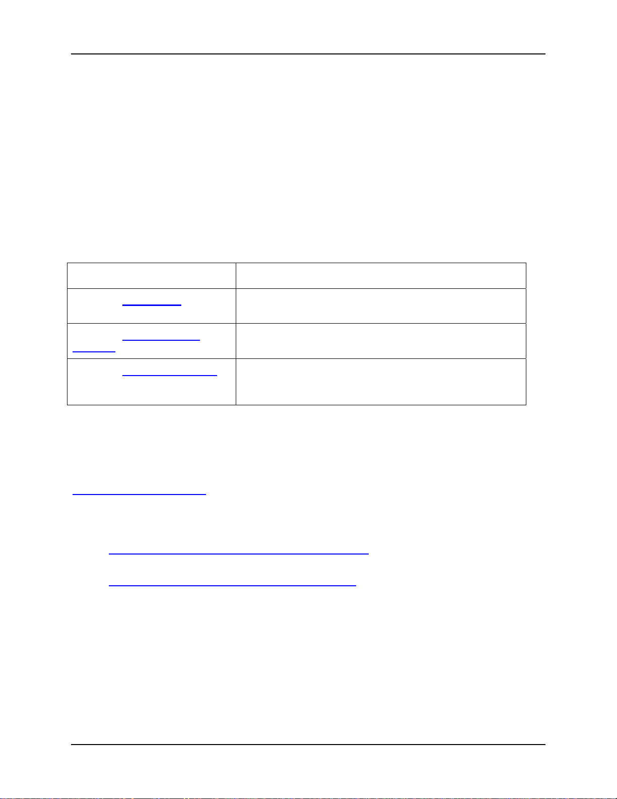
Chapter Description

Chapter 1: Introduction Contains descriptive information about OOIChem software

and a quick start procedure.

Chapter 2: Using OOIChem

Software

Chapter 3: Experiment Tutorial Contains procedures for taking measurements in Absorbance,

Provides installation and configuration instructions for
OOIChem software.

Transmission, Relative Irradiance, Concentration, and Kinetics
experiments.

Product-Related Documentation

You can access documentation for Ocean Optics products by visiting our website at

http://www.oceanoptics.com. Select Technical → Operating Instructions, then choose the appropriate

document from the available drop-down lists. Or, use the Search by Model Number field at the bottom
of the web page.

• Detailed instructions for the OOIBase32 Spectrometer Operating Software are located at:

http://www.oceanoptics.com/technical/ooibase32bit.pdf.

• Instructions for the OOIPS2000 Operating Software for the handheld PC are located at:

http://www.oceanoptics.com/products/ooips2000.asp.

Engineering-level documentation is located on our website at Technical → Engineering Docs.
You can also access operating instructions for Ocean Optics products from the Software and Technical

Resources CD that ships with the product.

105-00000-CHM-02-0405 PRELIMINARY DRAFT iii

About This Manual

Upgrades

Occasionally, you may find that you need Ocean Optics to make a change or an upgrade to your system.
To facilitate these changes, you must first contact Customer Support and obtain a Return Merchandise
Authorization (RMA) number. Please contact Ocean Optics for specific instructions when returning a
product.

OOIChem software will be updated and improved continuously. To obtain free upgrades, visit out web
site at www.oceanoptics.com/products/Software.asp. To download free upgrades, you will need the
following password: hG59mP236I

iv PRELIMINARY DRAFT 105-00000-CHM-02-0405

Chapter 1

Introduction

Company History

Ocean Optics miniature fiber optic spectrometers and accessories have revolutionized the analytical
instrumentation market by dramatically reducing the size and cost of optical sensing systems. More than
10,000 Ocean Optics spectrometers have been sold worldwide -- striking evidence of the far-reaching
impact of low-cost, miniature components for fiber optic spectroscopy. Diverse fields such as research
and development, industrial process control, medical diagnostics, environmental monitoring and of
course, education have benefited from access to Ocean Optics technology.

In fact, Ocean Optics has its roots in education. It formed in 1989 when Florida university researchers
developed a fiber optic pH sensor as part of an instrument designed to study the role of the oceans in
global warming. The researchers soon formed Ocean Optics, Inc. and their ingenious work earned a Small
Business Innovation Research grant from the U.S. Department of Energy. While designing the pH­monitoring instrument, the researchers wanted to incorporate with their sensor a spectrometer small
enough to fit onto a buoy and were surprised to discover none existed. So, they built their own.

In 1992, the founders of Ocean Optics filled a substantial need in the research community and changed
the science of spectroscopy forever by introducing a breakthrough technology: the S1000 Miniature Fiber
Optic Spectrometer, nearly a thousand times smaller and ten times less expensive than previous systems.
Due to this dramatic reduction in size and cost of optical sensing systems, applications once deemed too
costly or impractical using conventional spectrometers were now feasible.

OOIChem Spectrometer Operating Software

OOIChem is a basic acquisition and display software that provides a real-time interface to a variety of
spectral-processing functions. OOIChem allows users to perform basic spectroscopic measurements such
as absorbance, transmission, relative irradiance, and concentration. OOIChem operates with Windows
95/98/Me/XP and Windows NT/2000. Visit our website at

www.OceanOptics.com/products/software.asp to download free OOIChem upgrades.

105-00000-CHM-02-0405 PRELIMINARY DRAFT 1

1: Introduction

OOIBase32 Spectrometer Operating Software

OOIBase32 is our standard spectrometer operating software that we provide free of charge to all
customers. While OOIChem is a basic acquisition and display program, OOIBase32 is user-customizable
and a much more advanced acquisition and display program. With OOIBase32 you have the ability to
control all system parameters; collect data from up to 8 spectrometer channels simultaneously and display
the results in a single spectral window; perform reference monitoring and time acquisition experiments;
and use numerous editing, viewing and spectral processing functions. At any time, users can receive free
OOIBase32 updates from our web site at

Ocean Optics also offers a complete line of light sources, sampling holders, in-line filter holders, flow
cells, and other sampling devices; an extensive line of optical fibers and probes; and collimating lenses,
attenuators, diffuse reflectance standards and integrating spheres. All components have SMA terminations
so that changing the sampling system is as easy as unscrewing a connector and adding a new component
or accessory.

This modular approach -- components are easily mixed and matched -- offers remarkable applications
flexibility. Users pick and choose from hundreds of products to create distinctive systems for an almost
endless variety of optical-sensing applications

www.OceanOptics.com/products/software.asp.

Packing List

A packing list comes with each order. It is located inside a plastic bag attached to the outside of the
shipment box. The invoice is mailed separately. The items listed on your packing slip include all of the
components in your order. However, some items on your packing list are actually items installed into
your spectrometer, such as the grating and slit. The packing list also includes important information such
as the shipping address, billing address, and components on back order.

Quick Start

Step 1: Install OOIChem Software

► Procedure

Before installing OOIChem, make sure that no other applications are running.

1. Insert the software CD into your floppy drive. Execute Setup.exe.

2. At the Welcome dialog box, click Next.

3. At the Destination Location dialog box, select a destination directory. Click Next.

4. At the Backup Replaced Files dialog box, select either Yes or No. Selecting Yes is
recommended and enables you to choose a destination directory. Click Next.

2 PRELIMINARY DRAFT 105-00000-CHM-02-0405

1: Introduction

5. Select a Program Manager Group. Click Next. At the Start Installation dialog box, click
Next.

6. At the Installation Complete dialog box, choose Finish.

7. When prompted to do so, restart your computer when the installation is complete.

Step 2: Configure OOIChem Software

After you restart your computer, navigate to the OOIChem icon and select it. The first time you run
OOIChem after installation, you must follow several prompts to configure your system before taking
measurements.

Hardware Configuration

The Configure Hardware dialog box opens when you first run OOIChem. The parameters in this dialog
box are usually set only once – when OOIChem is first installed and the software first opens.

Procedure

►

1. Under Spectrometer Type, choose S4000.

2. Under A/D Converter Type, choose HR4000.

3. In the USB Serial Number field, select the serial number of the HR4000 spectrometer in
your Maxwell system from the drop-down list.

4. For your setup, only these parameters apply to your system. Click OK. You can always
change these settings once OOIChem is fully operational by selecting Spectrometer |
Hardware Configuration.

Spectrometer Configuration

At this point, OOIChem should be acquiring data from your spectrometer. There should be a dynamic
trace responding to light near the bottom of the displayed graph. Now that OOIChem is running, you need
to configure your system. Select Spectrometer | Spectrometer Configuration from the menu.

• Coefficients. Loaded automatically from the spectrometer.

• Trigger mode. Select No External Trigger, unless you have wired an external triggering device

to the spectrometer for synchronizing data with an external event.

• Graph and chart display mode. Choose Spectrum Only to only view live spectra from one
spectrometer channel. Choose Spectrum & Kinetics to view both real-time live spectra in the top
half of the graph and to view a chart displaying your kinetics experiment in the bottom half of the
graph.

• Flash Delay. This function is for use with a strobe light source. The Maxwell system does not
come with a strobe light source.

105-00000-CHM-02-0405 PRELIMINARY DRAFT 3

1: Introduction

• Color Temperature. Enter the color temperature of your reference light source used in relative
irradiance measurements.

Acquisition Parameters

Set data acquisition parameters by choosing an integration period and selecting averaging and boxcar
smoothing values.

Text Box

Enter the operator name, or any other identifying text here. This text appears in your data files. You can
edit this text at any time.

Step 3: Receive Data

Run OOIChem in Scope Mode and take a reference spectrum and a dark spectrum (see Experiment

Tutorial

sample measurements.

for details). Choose the absorbance, transmission, or relative irradiance mode to take your

4 PRELIMINARY DRAFT 105-00000-CHM-02-0405

Chapter 2

Using OOIChem Software

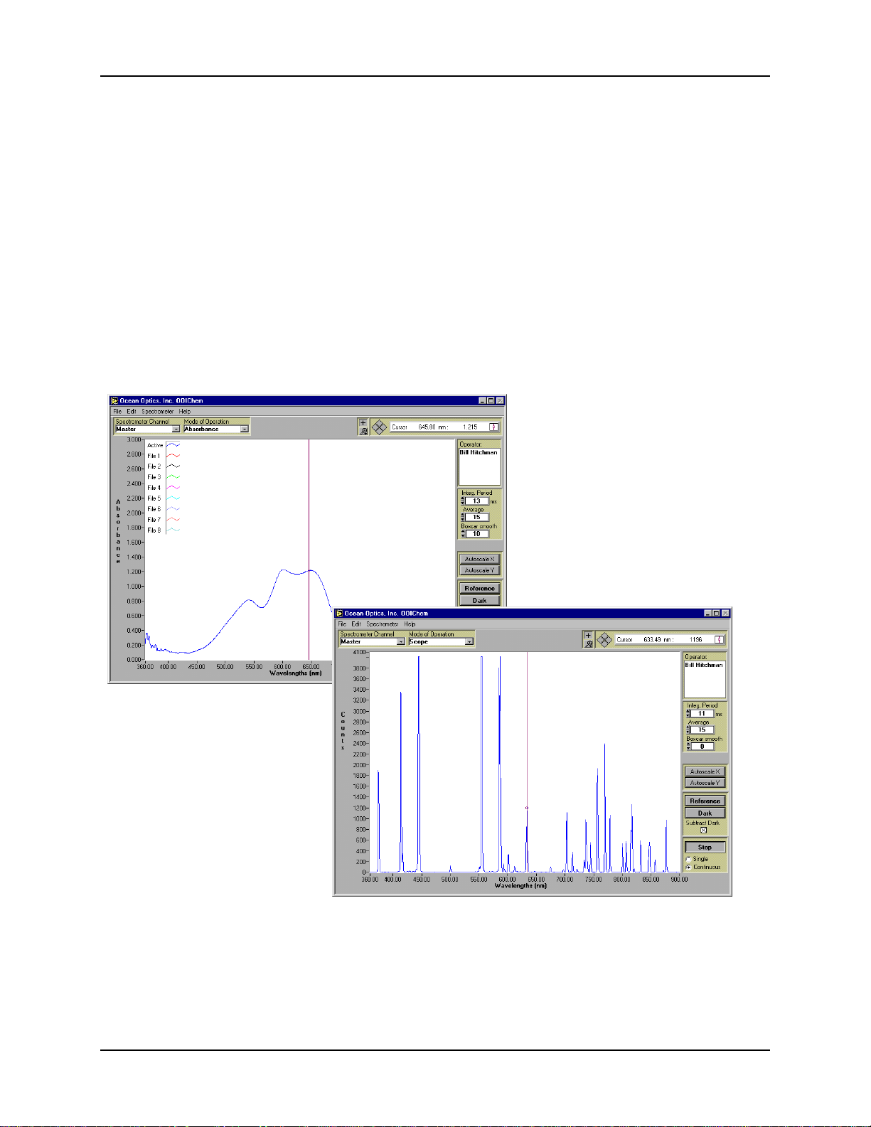
OOIChem software provides users with five different modes of operation: Scope, Absorbance,
Transmission, Relative Irradiance, and Concentration. In addition, the software allows users to control
data acquisition features such as integration period, averaging, and boxcar smoothing -- directly from the
spectral graph display. Users can acquire data by taking manual single scans or by running continuous
scans, and add into the spectral window as many as 8 previously saved overlay spectra.

Users can also perform kinetics
experiments, which allows users to
monitor and report up to 4 single
wavelengths or up to 2 calculated
values from a combination of
wavelengths – for example, an
absorbance value of 400 minus an
absorbance value of 700. A kinetics
chart displays the time series. When
the experiment is complete, the data
can be exported to an ASCII file for
additional processing.

Another exciting feature of
OOIChem is that users can control
the parameters for all system
functions such as acquiring data,
designing the graph display, and
configuring the cursor. Additional
features of OOIChem include the
ability to save data as ASCII files
and to store and retrieve sample
spectra.

If you find that you need more
advanced spectrometer operating
software, we have included, free of charge, OOIBase32, a sophisticated, 32-bit, user-customizable
advanced acquisition program. See the included OOIBase32 manual for a list of functions and features.

105-00000-CHM-02-0405

PRELIMINARY DRAFT 5

2: Using OOIChem Software

Display Functions

Several functions are accessed not through the menu but through buttons and task bars directly on the
display screen, on the top and to the right of the graph area. (The resolution of your computer's monitor
must be 800 x 600 or better to view OOIChem software.) From the display screen, you can choose a
mode of operation, configure the cursor, configure the graph, enter acquisition parameters, choose a mode
to acquire data, take reference, dark, and sample scans of your sample, and scale the graph.

Spectrometer Channel Selection

The Spectrometer Channel area allows you to animate the window for a specific spectrometer channel.
The Maxwell is a single spectrometer channel system. Select Master.

Mode of Operation

Scope

The signal graphed in Scope Mode is the raw voltage coming out of the A/D converter. Once you open
OOIChem and it begins to acquire data, you see the raw voltage from the detector expressed in A/D
counts. This spectral view mode is unique to Ocean Optics. It allows you to control signal processing
functions before taking absorbance, transmission, and relative irradiance measurements. Be careful when
using this mode, as it represents a combination of several factors: the intensity
of the light source, the reflectivity of the grating and the mirrors in the
spectrometer, the transmission of the fibers, the response of the detector, and the
spectral characteristics of the sample.

Scope Mode should primarily be used when selecting signal acquisition
parameters such as integration period, averaging and boxcar smoothing; and
when taking dark and reference scans.

Absorbance

Selecting this mode switches the spectral window into Absorbance Mode. Before this can occur, both a
dark and reference scan must be stored in Scope Mode (see
calculated by the following equation. When this equation is evaluated for each pixel of the detector, the
absorbance spectrum is produced.

S

-D

λ

Aλ = - log

Where:

S = Sample intensity at wavelength λ
D = Dark intensity at wavelength λ
R = Reference intensity at wavelength λ

6 PRELIMINARY DRAFT 105-00000-CHM-02-0405

10

(

Rλ-D

λ

)

λ

Experiment Tutorial). Absorbance is

2: Using OOIChem Software

Transmission

Selecting this mode switches the spectral window into Transmission Mode. This is also the spectral
processing mode used for Reflection spectroscopy, as the math necessary to compute reflection is
identical to transmission. Before this can occur, both a dark and reference scan must be stored in Scope
Mode (see

Where:

S = Sample intensity at wavelength λ
D = Dark intensity at wavelength λ
R = Reference intensity at wavelength λ

Experiment Tutorial). The transmission of a solution is calculated by the following equation:

%Tλ=

Sλ - D
Rλ - D

λ

x 100%

λ

Relative Irradiance

Selecting this mode switches the spectral window into Relative Irradiance Mode. The reference spectrum
must be made in Scope Mode with a blackbody of known color temperature. (Maxwell users cannot make
relative irradiance measurements because the light source that comes with the system is not a blackbody
source with a known color temperature. Additional hardware must be purchased.) A dark spectrum is
usually obtained by preventing light from entering the fiber that connects to the spectrometer (see

Experiment Tutorial). Relative irradiance spectra are a measure of the intensity of a light source relative

to a reference emission source. Relative irradiance is calculated by the following equation:

S

- D

λ

λ

)

λ

Where:

I

λ=Bλ

(

Rλ - D

B = Relative energy of the reference calculated from the color temperature (in Kelvin)
S = Sample intensity at wavelength λ
D = Dark intensity at wavelength λ
R = Reference intensity at wavelength λ

Concentration

Concentration is the amount of a specified substance in a solution. Graphs of absorbance vs.
concentration are known as Beer’s Law plots. These are calculated by first measuring the light that is
absorbed from a series of solutions with different known concentrations. The length of the sample -- such
as the path length of our cuvette holder – and the wavelength chosen for monitoring the amount of light
absorbed, are constants. Then a linear plot derived from the scans of these standard solutions with known
concentrations is obtained. The plot is then used to determine the unknown concentrations of solutions.

Experiment Tutorial).

(see

105-00000-CHM-02-0405 PRELIMINARY DRAFT 7

2: Using OOIChem Software

The absorbance of a solution is related to the concentration of the species within it. The relationship,
known as Beer’s Law , is:

Aλ = ε

Where:

c l

λ

A = Absorbance at wavelength λ,

ε = Extinction coefficient of the absorbing species at wavelength λ
c = Concentration
l = Optical pathlength

Cursor Function Bar

+ Sign

When the + is selected, the pointer becomes a crosshair symbol, enabling you to drag the cursor around
the graph.

Magnify Symbols

When the magnify symbol is selected, you can choose from among 6 magnify
functions. The function chosen will remain in use until another magnify icon or
the crosshair symbol is selected. Clockwise, beginning with the top left symbol,
the magnify icons perform the following functions:

Magnifies a specific area by clicking and dragging a box around an area

Zooms in on the horizontal scale, but the vertical scale remains the same

Zooms in on the vertical scale, but the horizontal scale remains the same

Zooms in approximately one point vertical and horizontal, click once or press continuously

Zooms out approximately one point vertical and horizontal, click once or press continuously

Reverts to the last zoom function

Cursor Diamond

To move the cursor left or right in small increments in the graph area, click on the left and right
sections of the move cursor diamond. The top and bottom sections of the diamond will send the
cursor to the next or previous channel in your system. (The Maxwell is a single channel system.

However, additional channels can be purchased at any time.)

8 PRELIMINARY DRAFT 105-00000-CHM-02-0405

2: Using OOIChem Software

Cursor Properties

In this toolbar, you can label the cursor and monitor the cursor’s X value and Y value. To the right of the
X and Y values of the cursor is a cursor selection button that
allows you to choose a cursor style and a point style. You can
also choose a color for the cursor and whether or not to display
the name of the channel the cursor is currently reporting.
Finally, you can bring the cursor to the center of the spectrum
or center the spectrum around the cursor’s current position.

Text Box

This box allows you to enter an operator name and any other text to identify your experiment. This text
appears in your data files. You can edit this text at any time.

Acquisition Parameters

Integration Period

Enter a value to set the integration period in milliseconds for an active
spectrometer channel. The integration period of the spectrometer is analogous to
the shutter speed of a camera. The higher the value specified for the integration
period, the longer the detector “looks” at the incoming photons. If your scope
mode intensity is too low, increase this value. If the intensity is too high, decrease
the value. While watching the graph trace in Scope Mode, adjust the integration
period and other acquisition parameters until the signal intensity level is
approximately 3500 counts.

Average

Enter a value to implement a sample averaging function that averages the specified number of spectra.
The higher the value entered the better the signal-to-noise ratio. The S:N improves by the square root of
the number of scans averaged.

Boxcar Smooth

Enter a value to implement a boxcar smoothing technique that averages across spectral data. This method
averages a group of adjacent detector elements. A value of 5, for example, averages each data point with
5 points (or bins) to its left and 5 points to its right. The greater this value, the smoother the data and the
higher the signal-to-noise ratio . However, if the value entered is too high, a loss in spectral resolution
results. The S:N improves by the square root of the number of pixels averaged.

Reference Scan

Selecting the Reference button activates a prompt to make sure your light is on. You then must choose to
either Store or Cancel your reference scan. A reference spectrum is taken with the light source on and a

105-00000-CHM-02-0405 PRELIMINARY DRAFT 9

2: Using OOIChem Software

blank in the sampling region. Storing a reference spectrum is requisite before the software can calculate
absorbance, transmission, and relative irradiance spectra. This command merely stores a reference
spectrum. To permanently save the reference spectrum to disk, select File | Save Spectral Values from
the menu.

Dark Scan

Selecting the Dark button activates a prompt to make sure the light path is
blocked. You then must choose to either Store or Cancel your dark scan
spectrum is taken with the light path to the spectrometer blocked. Storing a dark
spectrum is requisite before the software can calculate absorbance, transmission,
and relative irradiance spectra. This command merely stores a dark spectrum. To permanently save the
reference spectrum to disk, select File | Save Spectral Values from the menu .

. A dark

Subtract Dark

Selecting this box subtracts the current dark spectrum from the spectra being displayed. This command is
useful if you are trying to look at a change in an emission spectrum or are trying to eliminate from the
spectra fixed pattern noise caused by a very long integration period. The subtract dark spectrum function
only acts on spectra displayed in Scope Mode.

Acquire Data Modes

Chart Active

When Spectrum & Kinetics is chosen as the Graph and chart display mode in
the Spectrometer Configuration dialog box, the Chart Active function becomes
visible in the display area above the Scan button. This function is responsible only
for the Kinetics chart. By deselecting this function, users can use the scan button
and collect data in just the spectrum section of the graph. If the function is
enabled, choosing the scan button results in the collection of data in both the
spectrum section of the graph and the kinetics section of the graph.

Scan/Stop Button

When in Single mode, the Scan button acts as a snapshot. After selecting the Single mode, click on the
Scan button to take a scan. The button depresses and Stop replaces Scan. The button will stay depressed
until the scan has been completed (the time set in the Integration Period box).

When in Continuous mode, the Scan button continuously takes scans. After each integration cycle,
another scan will immediately begin. The button depresses and Stop replaces Scan. Click on Stop to halt
the scanning process and discontinue acquiring data.

10 PRELIMINARY DRAFT 105-00000-CHM-02-0405

2: Using OOIChem Software

Scaling the Graph

You can change the vertical and/or horizontal scales of the graph by simply clicking on an X and Y
endpoint and manually typing in a value. The graph will then resize itself.

File Menu Functions

Save Spectral Values

Select File | Save Spectral Values from the menu to save the current spectrum. Text box entries and
acquisition parameters are included in the headers of these files. You can then use these files as overlays
or import them into other software programs, such as Microsoft Excel.

Save Kinetics Values

Select File | Save Kinetics Values from the menu to save kinetics data. Text box entries and acquisition
parameters are included in the headers of these files. You can then import them into other software
programs, such as Microsoft Excel.

Open Spectrum Overlay

Select File | Open Spectrum Overlay from the menu to open a dialog box that allows you to open a
previously saved spectrum and to open it as an overlay (a static spectrum) while still acquiring live data.
You can open up to 8 overlays in the graph.

Open Kinetics Values

Select File | Open Kinetics Values from the menu to open a dialog box that allows you to open a
previously saved kinetics chart.

Printer Setup

Select File | Printer Setup from the menu to select and configure a printer for printing graphical spectra
or kinetics data.

Print Spectra and Kinetics

Select File | Print Spectra from the menu to print a spectrum, or select File | Print Kinetics from the
menu to print kinetics data.

105-00000-CHM-02-0405 PRELIMINARY DRAFT 11

2: Using OOIChem Software

Exit

Select File | Exit from the menu to quit OOIChem. A message box appears asking you if you are sure you
want to exit the software.

Edit Menu Functions

Clear Spectrum Overlays

Select Edit | Clear Spectrum Overlays from the menu to remove static spectra from the graph.

Clear Kinetics Values

Select Edit | Clear Kinetics Values from the menu to clear both the kinetics values from the chart and to
clear the kinetics traces. A message box then appears, asking if you are sure you want to clear the kinetics
chart.

Autoscale X

The Autoscale X function automatically adjusts the horizontal scale of a current graph so the
entire horizontal spectrum fills the display area.

Autoscale Y

The Autoscale Y function automatically adjusts the vertical scale of a current graph so the entire vertical
spectrum fills the display area.

Show Kinetics Values

When setting up your kinetics experiment, you must first select Spectrometer | Spectrometer
Configuration from the menu and make sure that Spectrum & Kinetics is selected next to Graph and

chart display mode. Then configure your experiment by selecting Spectrometer | Kinetics
Configuration from the menu. When you select your wavelengths, the values from these wavelengths

will be displayed above the kinetics chart if this function is enabled.

12 PRELIMINARY DRAFT 105-00000-CHM-02-0405

2: Using OOIChem Software

Show Legends

Select Edit | Show Legends to enable or disable the legends for the spectral trace,
overlays, and kinetics traces. When the legends are displayed, you can opt to
configure the traces by simply clicking on the legend trace you want to configure.
You have the opportunity to choose from several aesthetic functions such as: the
plot design of the spectrum, the point style used in the spectrum, the line style and
width desired, color of the plot, and a bar plot design. You can also choose to fill the
baseline in the spectrum. Utilize this function to differentiate one spectral trace from
another.

Spectrometer Menu Functions

Scan

When the Single mode is selected in the display screen, the Scan menu function acts as a snapshot. After
selecting the Single mode, select Spectrometer | Scan from the menu to take one scan of the sample.
When the Continuous mode is selected in the display screen, select Spectrometer | Scan from the menu
to continuously take scans.

Select Concentration Wavelength

This function is used when calculating the unknown concentration of a substance in a solution. You select
this function after you take an absorbance measurement of a standard solution with a known
concentration. Choose the wavelength of the highest peak in your absorbance spectrum. Then select
Spectrometer | Calculate Calibration Curve from the menu and complete the rest of your concentration
experiment. See

Concentration Experiments for step-by-step instructions on calculating concentrations.

Calculate Calibration Curve

Concentration is the amount of a specified substance in a solution. In order to calculate concentration, you
must take absorbance measurements of a series of solutions with different known concentrations. The
length of the sample and the wavelength chosen for monitoring the amount of light absorbed are
constants. Then a linear plot from taking these scans is obtained. This Calibration Curve is used to
determine the unknown concentrations. See
calculating concentrations and on using this dialog box.

Concentration Experiments for step-by-step instructions on

105-00000-CHM-02-0405 PRELIMINARY DRAFT 13

2: Using OOIChem Software

Enable Strobe

This function allows you to enable or disable the triggering of external strobes through the spectrometer.
You would only select Spectrometer | Strobe Enable from the menu if you were operating an external
strobe source. The Maxwell system does not include a strobe light source. However, the light source that
comes with the Maxwell can be turned off and on through the software and this function.

Trigger Mode

With OOIChem Operating Software, you have two methods of acquiring data. In the No External
Trigger Mode (or Normal Mode), the spectrometer is “free running.” That is, the spectrometer is

continuously scanning, acquiring, and transferring data to your computer, according to parameters set in
the software. In this mode, however, there is no way to synchronize the scanning, acquiring and
transferring of data with an external event.

To synchronize data acquisition with an external event, the External Software Trigger Mode is
available. It involves connecting an external triggering device
external trigger to the spectrometer before the software receives the data. In this mode, the spectrometer is
“free running,” just as it is in the Normal Mode. The spectrometer is continually scanning and collecting
data. With each trigger, the data collected during the integration period is transferred to the software. All
acquisition parameters, such as the integration period, are still set in the software. You should use this
mode if you are using a continuous light source and its intensity is constant before, during and after the
trigger.

2

to the spectrometer and then applying an

Note

To use the External Software Triggering option, it is imperative that you know the
specifications and limitations of your triggering device. The design of your triggering
device may prevent you from using the external software triggering mode as it is
described here.

► Procedure

To use the External Software Trigger Mode:

1. Supply a line from your triggering device to Pin 3 of the

J2 Accessory Connector on the spectrometer to provide
the positive voltage +5VDC to the spectrometer. (See
figure for pin location.) We do not advise using an
outside source to supply the voltage, as it is based on a
referenced ground and your reference may be different
from ours. Using Pin 3 to supply voltage ensures that the

spectrometer will receive the appropriate voltage for the trigger event.

J2 (D-SUB-15) Accessory Connector (female)

14

PRELIMINARY DRAFT 105-00000-CHM-02-0405

2: Using OOIChem Software

2. Supply a line from Pin 8 of the J2 Accessory Connector to your triggering device. (See figure for
pin location.)

3. Set your acquisition parameters in the software.

4. Select Spectrometer | Spectrometer Configuration from the menu and choose External
Software Trigger.

5. Once you select External Software Trigger, it will appear on your computer that your
spectrometer is unresponsive. Instead, it is waiting for the trigger. Activate your triggering
device.

Graph and Chart Display Mode

If you choose Spectrum Only, spectra from one real-time spectrometer channel and up to 8 overlays can
be displayed in the graph area. If you choose Spectrum & Kinetics, spectra from one real-time
spectrometer channel and up to 8 overlays can be displayed in the in the top half of the graph area. A
kinetics chart monitoring values from up to 4 wavelengths and 2 of their arithmetic calculations can be
displayed in the in the bottom half of the graph area, if the Chart Active function is enabled.

Flash Delay

The value entered here sets the delay, in milliseconds, between strobe signals sent out of the spectrometer.
This function allows you to enable or disable the triggering of external strobes through the spectrometer.
You would only enter a value in this box if you were operating an external strobe source. The Maxwell
system does not include a strobe light source.

Color Temperature

This box allows you to enter the color temperature (in Kelvin) of your light source. In order to calculate
relative irradiance, the reference spectrum must be made in Scope Mode with a blackbody light source of
known color temperature. This data is necessary for the software to complete calculations for relative
irradiance measurements. Maxwell users must purchase additional hardware to make relative irradiance
measurements.

Kinetics Configuration

Select Spectrometer | Kinetics Configuration from the menu to configure and establish the parameters
for a kinetics experiment. In the Kinetics Configuration dialog box, you can collect spectral data as a
function of time, from up to 4 single wavelengths and up to two mathematical combinations of these
wavelengths.

Data from a kinetics experiment will not be displayed in the graph unless you choose Spectrometer |

Spectrometer Configuration from the menu and select Spectrum & Kinetics next to Graph and chart
display mode. This way, not only will your kinetics experiment be displayed in the bottom half of the

graph area, you will also still see real-time spectra in the top half of the graph area.

105-00000-CHM-02-0405 PRELIMINARY DRAFT 15

2: Using OOIChem Software

Preset Duration

Enter a value to set the length of time for
the entire kinetics process. Be sure to
select hours, minutes and seconds. Your
kinetics experiment cannot exceed a
duration of 24 hours.

Preset Sampling Interval

Enter a value to set the frequency of the
data collected in a kinetics process. Be
sure to select hours, minutes and seconds.

Wavelength

Enter the single wavelengths from which you wish to collect data. You can collect data from up to 4
single wavelengths, characterized as

a, b, c, and d.

Display

If you want the data graphed from these single wavelengths, or from the mathematical calculations of
these wavelengths (described below), select the display box to the right of your values.

Mathematical Calculations

In the boxes next to x = and y =, you have the opportunity to perform calculations on the data collected
from the single wavelengths you specified as
which represents the calculation used in the box next to

a, b, c, and d. Also in the box next to y =, you can use x,

x =.

16 PRELIMINARY DRAFT 105-00000-CHM-02-0405

Chapter 3

Experiment Tutorial

Overview

When you are ready to begin your experiment, you should have already installed the Maxwell and
OOIChem software. Now you are ready to take your measurements. Because of the components making
up your Maxwell system, it is ideal for absorbance and transmission. The Maxwell system can also make
relative irradiance measurements. If, however, you wish to use your system for other measuring functions,
additional products might be required. Contact an Ocean Optics Applications Scientist for options.

Absorbance Experiments

Absorbance spectra are a measure of how much light is absorbed by a sample. The software calculates
absorbance (

Where:

S = Sample intensity at wavelength λ
D = Dark intensity at wavelength λ
R = Reference intensity at wavelength λ

Common applications include the quantification of chemical concentrations in aqueous or gaseous
samples.

Aλ) using the following equation:

S

-D

λ

Aλ = - log

10

(

Rλ-D

λ

)

λ

105-00000-CHM-02-0405 PRELIMINARY DRAFT 17

3: Experiment Tutorial

Procedure

►

To take an absorbance measurement:

1. Select Scope under Mode of Operation in the software display area. Make sure the signal is on
scale. Adjust acquisition parameters so that the peak intensity of the reference signal is about
3500 counts. Take a reference spectrum by first making sure nothing is blocking the light path
going to your spectrometer. The analyte you want to measure must be absent while taking a
reference spectrum. Take the reference reading by clicking the Reference button in the software
display area. (This command merely stores a reference spectrum. To save a spectrum, you must
select File | Save Spectral Values from the menu.) Storing a reference spectrum is required
before the software can calculate absorbance spectra.

2. While still in Scope Mode, take a dark spectrum by first completely blocking the light path going
to your spectrometer. (If possible, do not turn off the light source. If you must turn off your light
source to store a dark spectrum, make sure to allow enough time for the lamp to warm up before
continuing your experiment.) Take the dark reading by clicking the Dark button in the software
display area. (This command merely stores a dark spectrum. To save a spectrum, you must select
File | Save Spectral Values from the menu.) Storing a dark spectrum is requisite before the
software can calculate absorbance spectra.

3. Begin an absorbance measurement by first making sure the sample is in place and nothing is
blocking the light going to your sample. Then select Absorbance under Mode of Operation in
the software display area. Click on the Scan button in the display area to take a scan. If Single is
selected, only one scan will be taken. If Continuous is selected, the spectrometer will
continuously take scans until you click on the Stop button. To save the spectrum, select File |
Save Spectral Values from the menu.

Note

If at any time any sampling variable changes – including integration period, averaging,
boxcar smoothing, distance from light source to sample, etc. – you must store a new
reference and dark spectrum.

Transmission Experiments

Transmission is the percentage of energy passing through a system relative to the amount that passes
through the reference. Transmission Mode is also used to show the portion of light reflected from a
sample. Transmission and reflection measurements require the same mathematical calculation. The
transmission is expressed as a percentage (

%Tλ) relative to a standard substance (such as air).

18 PRELIMINARY DRAFT 105-00000-CHM-02-0405

3: Experiment Tutorial

The software calculates %Tλ (or %Rλ) by the following equation:

%Tλ=

Sλ - D
R

- D

λ

λ

x 100%

λ

Where:

S = Sample intensity at wavelength λ
D = Dark intensity at wavelength λ

R = Reference intensity at wavelength λ
Common applications include measurement of transmission of light through solutions, optical filters,

optical coatings, and other optical elements such as lenses and fibers.

Note

For transmission of light through solutions, we offer a transmission dip probe with screw­on, removable tips in 2-mm, 5-mm or 10-mm path lengths. Contact Ocean Optics for
more information.

► Procedure

To take a transmission measurement:

1. Select Scope under Mode of Operation in the software display area. Make sure the signal is on
scale. Adjust acquisition parameters so that the peak intensity of the reference signal is about
3500 counts. Take a reference spectrum by first making sure nothing is blocking the light path
going to your spectrometer. The analyte you want to measure must be absent while taking a
reference spectrum. Take the reference reading by clicking the Reference button in the software
display area. (This command merely stores a reference spectrum. To save a spectrum, you must
select File | Save Spectral Values from the menu.) Storing a reference spectrum is requisite
before the software can calculate transmission spectra.

2. While still in Scope Mode, take a dark spectrum by first completely blocking the light path going
to your spectrometer. (If possible, do not turn off the light source. If you must turn off your light
source to store a dark spectrum, make sure to allow enough time for the lamp to warm up before
continuing your experiment.) Take the dark reading by clicking the Dark button in the software
display area. (This command merely stores a dark spectrum. To save a spectrum, you must select
File | Save Spectral Values from the menu.) Storing a dark spectrum is requisite before the
software can calculate transmission spectra.

3. Begin a transmission measurement by first making sure the sample is in place and nothing is
blocking the light going to your sample. Then select Transmission under Mode of Operation in
the software display area. Click on the Scan button in the display area to take a scan. If Single is
selected, only one scan will be taken. If Continuous is selected, the spectrometer will
continuously take scans until you click on the Stop button. To save the spectrum, select File |
Save Spectral Values from the menu.

105-00000-CHM-02-0405 PRELIMINARY DRAFT 19

3: Experiment Tutorial

Note

If at any time any sampling variable changes – including integration period, averaging,
boxcar smoothing, distance from light source to sample, etc. – you must store a new
reference and dark spectrum.

Relative Irradiance Experiments

Irradiance is the amount of energy at each wavelength from a radiant sample. In relative terms, it is the
fraction of energy from the sample compared to the energy collected from a lamp with a blackbody
energy distribution, normalized to 1 at the energy maximum. Relative irradiance is calculated by the
following equation:

- D

S

λ

I

λ=Bλ

Where:

B = Relative energy of the reference calculated from the color temperature (in Kelvin)

S = Sample intensity at wavelength λ
D = Dark intensity at wavelength λ
R = Reference intensity at wavelength λ

Common applications include characterizing the light output of LEDs, incandescent lamps and other
radiant energy sources such as sunlight. Also included in irradiance measurements is fluorescence, in
which case the spectrometer measures the energy given off by materials that have been excited by light at
a shorter wavelength.

(

Rλ - D

λ

)

λ

Note

The components that came with the Maxwell will not allow you to make relative
irradiance measurements. To make relative irradiance measurements, the reference
spectrum must be made in Scope Mode with a blackbody light source of known color
temperature. This color temperature is needed in order to calculate relative irradiance.
The light source that comes with the Maxwell is not a blackbody light source with a
known color. To purchase a blackbody light source and other necessary hardware, contact
Ocean Optics.

► Procedure

To take a relative irradiance measurement:

1. Select Spectrometer | Spectrometer Configuration from the menu. Next to Color Temp, make
sure the color temperature in Kelvin of the reference lamp you are going to use is entered here.
Click OK.

20 PRELIMINARY DRAFT 105-00000-CHM-02-0405

3: Experiment Tutorial

2. Select Scope under Mode of Operation in the software display area. Make sure the signal is on
scale by adjusting acquisition parameters. Take a reference spectrum of your reference lamp.
Take the reference reading by clicking the Reference button in the software display area. (This
command merely stores a reference spectrum. To save a spectrum, you must select File | Save
Spectral Values from the menu.) Storing a reference spectrum is requisite before the software
can calculate relative irradiance spectra.

3. While still in Scope Mode, take a dark spectrum by first completely blocking light from going to
your spectrometer. Take the dark reading by clicking the Dark button in the software display
area. (This command merely stores a dark spectrum. To save a spectrum, you must select File |
Save Spectral Values from the menu.) Storing a dark spectrum is requisite before the software
can calculate relative irradiance spectra.

4. Begin a relative irradiance measurement by first positioning the fiber at the light or emission
source you wish to measure. Then select Relative Irradiance under Mode of Operation in the
software display area. Click on the Scan button in the display area to take a scan. If Single is
selected, only one scan will be taken. If Continuous is selected, the spectrometer will
continuously take scans until you click on the Stop button. To save the spectrum, select File |
Save Spectral Values from the menu.

Note

If at any time any sampling variable changes – including integration period, averaging,
boxcar smoothing, distance from light source to sample, etc. – you must store a new
reference and dark spectrum.

Concentration Experiments

The absorbance of a solution is related to the concentration of the species within it. The relationship,
known as Beer’s Law , is:

Aλ = ε

Where:

A = Absorbance at wavelength λ,
ε = Extinction coefficient of the absorbing species at wavelength λ

c = Concentration
l = Optical pathlength

Concentration is the amount of a specified substance in a solution. Graphs of absorbance vs.
concentration are known as Beer’s Law plots. These are prepared by measuring the light absorbed by a
series of solutions with different known concentrations. The length of the sample -- such as the path
length of our cuvette holder -- and the wavelength chosen for monitoring the amount of light absorbed are
constants. A linear plot from taking scans of these standard solutions with known concentrations is then
obtained. The plot is then used to determine the unknown concentrations of substances in solutions.

c l

λ

105-00000-CHM-02-0405 PRELIMINARY DRAFT 21

3: Experiment Tutorial

To discover the unknown concentration of a substance in a solution, you must first take spectral scans of a
series of solutions with different known concentrations of the same substance. You begin this process by
taking an absorbance spectrum of the solution with the highest known concentration.

Procedure

►

1. Select Scope under Mode of Operation in the software display area. Make sure the signal is on
scale. Adjust acquisition parameters so that the peak intensity of the reference signal is about
3500 counts. Take a reference spectrum by first making sure nothing is blocking the light path
going to your spectrometer. The solution with the highest known concentration you want to
measure must be absent while taking a reference spectrum. Take the reference reading by clicking
the Reference button in the software display area. To save the spectrum, select File | Save
Spectral Values from the menu.

2. While still in Scope Mode, take a dark spectrum by first completely blocking the light path going
to your spectrometer. (If possible, do not turn off the light source. If you must turn off your light
source to store a dark spectrum, make sure to allow enough time for the lamp to warm up before
continuing your experiment.) Take the dark reading by clicking the Dark button in the software
display area. To save the spectrum, select File | Save Spectral Values from the menu.

3. Take the solution with the highest known concentration and put it in the cuvette holder. Make
sure nothing is blocking the light going to your sample. Then select Absorbance under Mode of
Operation. Click on the Scan button in the display area to take a scan. Make sure Single is
selected. To save the spectrum, select File | Save Spectral Values from the menu.

4. Now select the wavelength for monitoring the concentration of your solutions by choosing
Spectrometer | Select Concentration Wavelength from the menu. Move the cursor to the
highest absorbance peak of the spectrum of the solution with the highest known concentration and
choose Select.

5. Remove the solution with the highest known concentration. Select Spectrometer | Calculate a
Calibration Curve from the menu. The Calculate Calibration Curve dialog box opens. Now you
will begin taking scans of the rest of your series of standard solutions with known concentrations,
from the lowest known concentration to highest, all while working in this dialog box.

6. If you wish, you can take a new reference and a new dark scan for each solution by choosing
Scan | Dark and Scan | Reference from the menu of this dialog box. However, in this case, it is
not necessary. If no reference or dark scan is taken at this point, the software will use the
reference and dark scans taken in Steps 1 and 2 to calculate absorbance.

7. Take the solution with the lowest known concentration and put it in the cuvette holder. Enter the
known concentration of the standard solution in the chart in the Concentration column, next to
Solution #1.

22 PRELIMINARY DRAFT 105-00000-CHM-02-0405

3: Experiment Tutorial

8. Click the Scan button or select Scan | Solution from the menu. The absorbance value will appear
next to the concentration for Solution #1. At any point, you can select Edit | Clear from the menu
to clear the dialog box of all data.

9. Take Solution #1 out of the cuvette holder and put in another standard solution with the next
highest known concentration. Enter the known concentration of the standard solution in the chart
in the Concentration column, next to Solution #2.

10. Click the Scan button or select Scan | Solution from the menu. The absorbance value will appear
next to the concentration for Solution #2.

11. You may continue to scan solutions with known concentrations. You must scan at least 2 in order
to achieve a calibration curve.

12. When you have completed taking scans of your solutions with known concentrations, click the
View Calibration Curve button. You will then have the Intercept and Slope of your curve. The

Slope is the ε necessary to compute Beer’s Law and to find the unknown concentration of a
solution.

13. At this time, you may also select a label for your concentration values, such at Moles per Liter,
in the Concentration Units box. This is only a label and does not affect the data in any way.

105-00000-CHM-02-0405 PRELIMINARY DRAFT 23

3: Experiment Tutorial

14. Select Edit | Show Legend from the menu to display the legend for the calibration curve. The
legend allows you to choose a plot design, point style, line style, line width and plot color. Select
Edit | Show Palette from the menu to display a variety of options for configuring the curve. The
palette provides features such as autoscaling, graph formatting, value precision, mode mapping,
and graph positioning.

15. You can select File | Print from the menu for the dialog box to print the dialog box. To save the
current calibration curve data, select File | Save from the menu for the dialog box.

16. Select File | Close from the menu for the dialog box to close this dialog box and return to the
main window.

17. When a message box asks if you would like to use this calibration curve when calculating
concentration values, select Yes.

18. Now that you are back in the main display window, place the solution with the unknown
concentration of a substance in the cuvette holder.

19. Under Mode of Operation, select Concentration. Click the Scan button to receive your
concentration values.

Kinetics Experiments

Select Spectrometer | Kinetics Configuration from the menu to configure and establish the parameters
for a kinetics experiment. In the Kinetics Configuration dialog box, you can collect spectral data as a
function of time, from up to 4 single
wavelengths and up to two mathematical
combinations of these wavelengths.

A kinetics experiment will not be
displayed in the graph unless you choose

Spectrometer | Spectrometer
Configuration from the menu and
choose Spectrum & Kinetics next to
Graph and chart display mode. This

way, not only will your kinetics
experiment be displayed in the bottom
half of the graph area, you will also still
see a spectrometer channel’s real-time
spectra in the top half of the graph area.

►

Procedure

To run a kinetics experiment:

1. In the graph area, select acquisition parameters, such as integration period, averaging, and boxcar
smoothing values. Do not change these parameters for the duration of the kinetics experiment.

24 PRELIMINARY DRAFT 105-00000-CHM-02-0405

3: Experiment Tutorial

2. Select Spectrometer | Kinetics Configuration from the menu to open the Kinetics Configuration
dialog box.

3. Enter a Preset Duration value to set the length of time for the entire kinetics process. Be sure to
select hours, minutes and seconds. The duration of your kinetics experiment cannot exceed 24
hours.

4. Enter a Preset Sampling Interval value to set the frequency of the data collected in a kinetics
process. Be sure to select hours, minutes and seconds. Data from a timed acquisition is stamped
with a time that is accurate to 1 millisecond.

5. Under Wavelength, enter the single wavelengths from which you wish to collect data. You can
collect data from up to 4 single wavelengths, characterized as a, b, c, and d.

6. If you want the data graphed from these single wavelengths, or from the mathematical
calculations (described in the next step), select the Display box to the right of your values.

7. In the boxes next to
collected from the single wavelengths you specified as

x, which represents the calculation used in x =.

use

x = and y =, you have the opportunity to perform calculations on the data

a, b, c, and d. In the y = box, you can also

8. Click OK to confirm the parameters and close the dialog box.

9. Click the Scan button to begin the kinetics experiment. Make sure that Continuous is selected.
The top half of the graph displays a real-time full wavelength spectrum. The bottom half of the
graph displays the data for the selected wavelengths and their derived arithmetic calculations.
Each data set is stored with a time stamp.

10. Click the Stop button to stop the experiment. However, if a Preset Duration time was selected,
the experiment will automatically stop after the designated time has passed.

11. Select File | Save Kinetics Values from the menu to save a tab-delimited ASCII file with the
spectrometer’s serial number, active channel and acquisition parameters in a header. This file can
be opened with any text or spreadsheet editor.

105-00000-CHM-02-0405 PRELIMINARY DRAFT 25

3: Experiment Tutorial

26 PRELIMINARY DRAFT 105-00000-CHM-02-0405

Index

A

absorbance experiment, 17
Absorbance mode, 6
Acquire Data modes, 10

Chart Active, 10

Acquisition parameters, 9

Average, 9
Boxcar Smooth, 9
Integration Period, 9

Autoscale

X, 12
Y, 12

C

Calculate Calibration Curve, 13
Chart Active, 10
Clear Kinetic Values, 12
Clear Spectrum Overlays, 12
Color Temperature, 15
company history, 1
concentration experiment, 21
Concentration mode, 7
configure

hardware, 3
spectrometer, 3

cursor

+ sign, 8
diamond, 8
magnify symbols, 8
properties, 9

cursor function bar, 8

D

Dark Scan, 10
data

receiving, 4
Display, 16
Display functions, 6
document

audience, iii

purpose, iii

summary, iii

E

Edit Menu functions, 12

Autoscale X, 12

Autoscale Y, 12

Clear Kinetic Values, 12

Clear Spectrum Overlays, 12

Show Kinetics Values, 12

Show Legends, 13
Enable Strobe, 14
Exit, 12
experiment tutorial, 17

absorbance, 17

concentration, 21

kinetics, 24

relative irradiance, 20

transmission, 18

105-00000-CHM-02-0405

PRELIMINARY DRAFT 27

Index

F

File Menu functions, 11

Exit, 12
Open Kinetics Values, 11
Open Spectral Overlay, 11
Print Spectra and Kinetics, 11
Printer Setup, 11
Save Kinetic Values, 11
Save Spectral Values, 11

Flash Delay, 15

G

graph

scaling, 11

Graph and Chart Display mode, 15

H

hardware

configuration, 3

K

Kinetic Values, 11
Kinetics Configuration, 15

Display, 16
Mathematical Calculations, 16
Preset Duration, 16
Preset Sampling Interval, 16
Wavelength, 16

kinetics experiment, 24

O

OOIBase32 Operating Software

overview, 2
OOIChem Software, 5

overview, 1
Open Kinetics Values, 11
Open Spectral Overlay, 11
operation mode, 6

Absorbance, 6

Concentration, 7

Relative Irradiance, 7

Scope, 6

Transmission, 7
overview

OOIBase32 Operating Software, 2

OOIChem Software, 1

P

packing list, 2
Preset Duration, 16
Preset Sampling Interval, 16
Print Spectra and Kinetics, 11
Printer Setup, 11
procedure

quick start, 2
product-related documentation, iii

Q

quick start, 2

R

M

Mathematical Calculations, 16

28

Reference Scan, 9
relative irradiance experiment, 20
Relative Irradiance mode, 7

PRELIMINARY DRAFT 105-00000-CHM-02-0405

Index

S

scaling the graph, 11
scan

dark, 10

reference, 9
Scan, 13
Scan/Stop button, 10
Scope mode, 6
Select Concentration Wavelength, 13
Show Kinetics Values, 12
Show Legends, 13
Spectral Values, 11
spectrometer

configuration, 3
spectrometer channel selection, 6
Spectrometer Menu functions, 13

Calculate Calibration Curve, 13

Enable Strobe, 14

Kinetics Configuration, 15

Scan, 13

Select Concentration Wavelength, 13
Subtract Dark, 10

T

text box, 9
transmission experiment, 18
Transmission mode, 7
Trigger mode, 14

U

upgrades, iv

W

Wavelength, 16

105-00000-CHM-02-0405

PRELIMINARY DRAFT 29

Index

30

PRELIMINARY DRAFT 105-00000-CHM-02-0405