NXP Semiconductors DSP56800E User Manual

Download

GMCLIB User's Guide

DSP56800E

Document Number: DSP56800EGMCLIBUG

Rev. 2, 10/2015

GMCLIB User's Guide, Rev. 2, 10/2015

2 Freescale Semiconductor, Inc.

Contents

Section number Title Page

Chapter 1

Library

1.1 Introduction.................................................................................................................................................................... 5

1.2 Library integration into project (CodeWarrior™ Development Studio) .......................................................................7

Chapter 2

Algorithms in detail

2.1 GMCLIB_Clark..............................................................................................................................................................17

2.2 GMCLIB_ClarkInv........................................................................................................................................................ 18

2.3 GMCLIB_Park............................................................................................................................................................... 20

2.4 GMCLIB_ParkInv..........................................................................................................................................................21

2.5 GMCLIB_DecouplingPMSM........................................................................................................................................ 23

2.6 GMCLIB_ElimDcBusRipFOC...................................................................................................................................... 27

2.7 GMCLIB_ElimDcBusRip.............................................................................................................................................. 31

2.8 GMCLIB_SvmStd..........................................................................................................................................................36

2.9 GMCLIB_SvmIct...........................................................................................................................................................51

2.10 GMCLIB_SvmU0n........................................................................................................................................................ 55

2.11 GMCLIB_SvmU7n........................................................................................................................................................ 59

GMCLIB User's Guide, Rev. 2, 10/2015

Freescale Semiconductor, Inc. 3

GMCLIB User's Guide, Rev. 2, 10/2015

4 Freescale Semiconductor, Inc.

Chapter 1 Library

1.1 Introduction

1.1.1 Overview

This user's guide describes the General Motor Control Library (GMCLIB) for the family of DSP56800E core-based digital signal controllers. This library contains optimized functions.

1.1.2

Data types

GMCLIB supports several data types: (un)signed integer, fractional, and accumulator. The integer data types are useful for general-purpose computation; they are familiar to the MPU and MCU programmers. The fractional data types enable powerful numeric and digital-signal-processing algorithms to be implemented. The accumulator data type is a combination of both; that means it has the integer and fractional portions.

The following list shows the integer types defined in the libraries:

• Unsigned 16-bit integer —<0 ; 65535> with the minimum resolution of 1

• Signed 16-bit integer —<-32768 ; 32767> with the minimum resolution of 1

• Unsigned 32-bit integer —<0 ; 4294967295> with the minimum resolution of 1

• Signed 32-bit integer —<-2147483648 ; 2147483647> with the minimum resolution of 1

The following list shows the fractional types defined in the libraries:

• Fixed-point 16-bit fractional —<-1 ; 1 - 2

• Fixed-point 32-bit fractional —<-1 ; 1 - 2

-15

> with the minimum resolution of 2

-31

> with the minimum resolution of 2

-15

-31

GMCLIB User's Guide, Rev. 2, 10/2015

Freescale Semiconductor, Inc. 5

Introduction

The following list shows the accumulator types defined in the libraries:

• Fixed-point 16-bit accumulator —<-256.0 ; 256.0 - 2-7> with the minimum resolution of 2

• Fixed-point 32-bit accumulator —<-65536.0 ; 65536.0 - 2 resolution of 2

-7

-15

> with the minimum

1.1.3 API definition

GMCLIB uses the types mentioned in the previous section. To enable simple usage of the algorithms, their names use set prefixes and postfixes to distinguish the functions' versions. See the following example:

f32Result = MLIB_Mac_F32lss(f32Accum, f16Mult1, f16Mult2);

where the function is compiled from four parts:

• MLIB—this is the library prefix

• Mac—the function name—Multiply-Accumulate

• F32—the function output type

• lss—the types of the function inputs; if all the inputs have the same type as the output, the inputs are not marked

The input and output types are described in the following table:

Table 1-1. Input/output types

Type Output Input

frac16_t F16 s frac32_t F32 l acc32_t A32 a

1.1.4 Supported compilers

GMCLIB for the DSP56800E core is written in assembly language with C-callable interface. The library is built and tested using the following compilers:

• CodeWarrior™ Development Studio

For the CodeWarrior™ Development Studio, the library is delivered in the gmclib.lib file.

GMCLIB User's Guide, Rev. 2, 10/2015

6 Freescale Semiconductor, Inc.

Chapter 1 Library

The interfaces to the algorithms included in this library are combined into a single public interface include file, gmclib.h. This is done to lower the number of files required to be included in your application.

1.1.5 Special issues

1. The equations describing the algorithms are symbolic. If there is positive 1, the number is the closest number to 1 that the resolution of the used fractional type allows. If there are maximum or minimum values mentioned, check the range allowed by the type of the particular function version.

2. The library functions require the core saturation mode to be turned off, otherwise the results can be incorrect. Several specific library functions are immune to the setting of the saturation mode.

3. The library functions round the result (the API contains Rnd) to the nearest (two's complement rounding) or to the nearest even number (convergent round). The mode used depends on the core option mode register (OMR) setting. See the core manual for details.

4. All non-inline functions are implemented without storing any of the volatile registers (refer to the compiler manual) used by the respective routine. Only the non-volatile registers (C10, D10, R5) are saved by pushing the registers on the stack. Therefore, if the particular registers initialized before the library function call are to be used after the function call, it is necessary to save them manually.

1.2

Library integration into project (CodeWarrior™ Development Studio)

This section provides a step-by-step guide to quickly and easily integrate the GMCLIB into an empty project using CodeWarrior™ Development Studio. This example uses the MC56F8257 part, and the default installation path (C:\Freescale\FSLESL \DSP56800E_FSLESL_4.2) is supposed. If you have a different installation path, you must use that path instead.

1.2.1

To start working on an application, create a new project. If the project already exists and is open, skip to the next section. Follow the steps given below to create a new project.

1. Launch CodeWarrior™ Development Studio.

Freescale Semiconductor, Inc. 7

New project

GMCLIB User's Guide, Rev. 2, 10/2015

Library integration into project (CodeWarrior™ Development Studio)

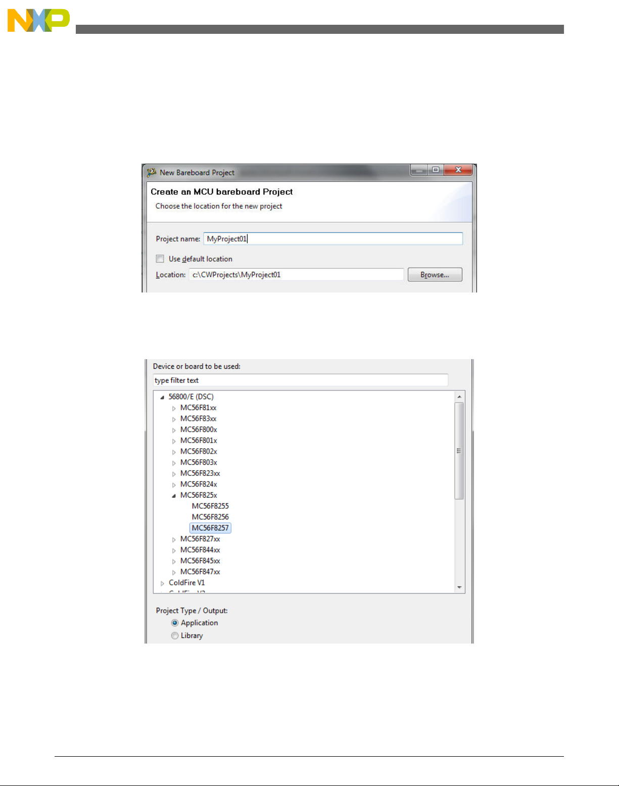
2. Choose File > New > Bareboard Project, so that the "New Bareboard Project" dialog appears.

3. Type a name of the project, for example, MyProject01.

4. If you don't use the default location, untick the “Use default location” checkbox, and type the path where you want to create the project folder; for example, C: \CWProjects\MyProject01, and click Next. See Figure 1-1.

Figure 1-1. Project name and location

5. Expand the tree by clicking the 56800/E (DSC) and MC56F8257. Select the Application option and click Next. See Figure 1-2.

Figure 1-2. Processor selection

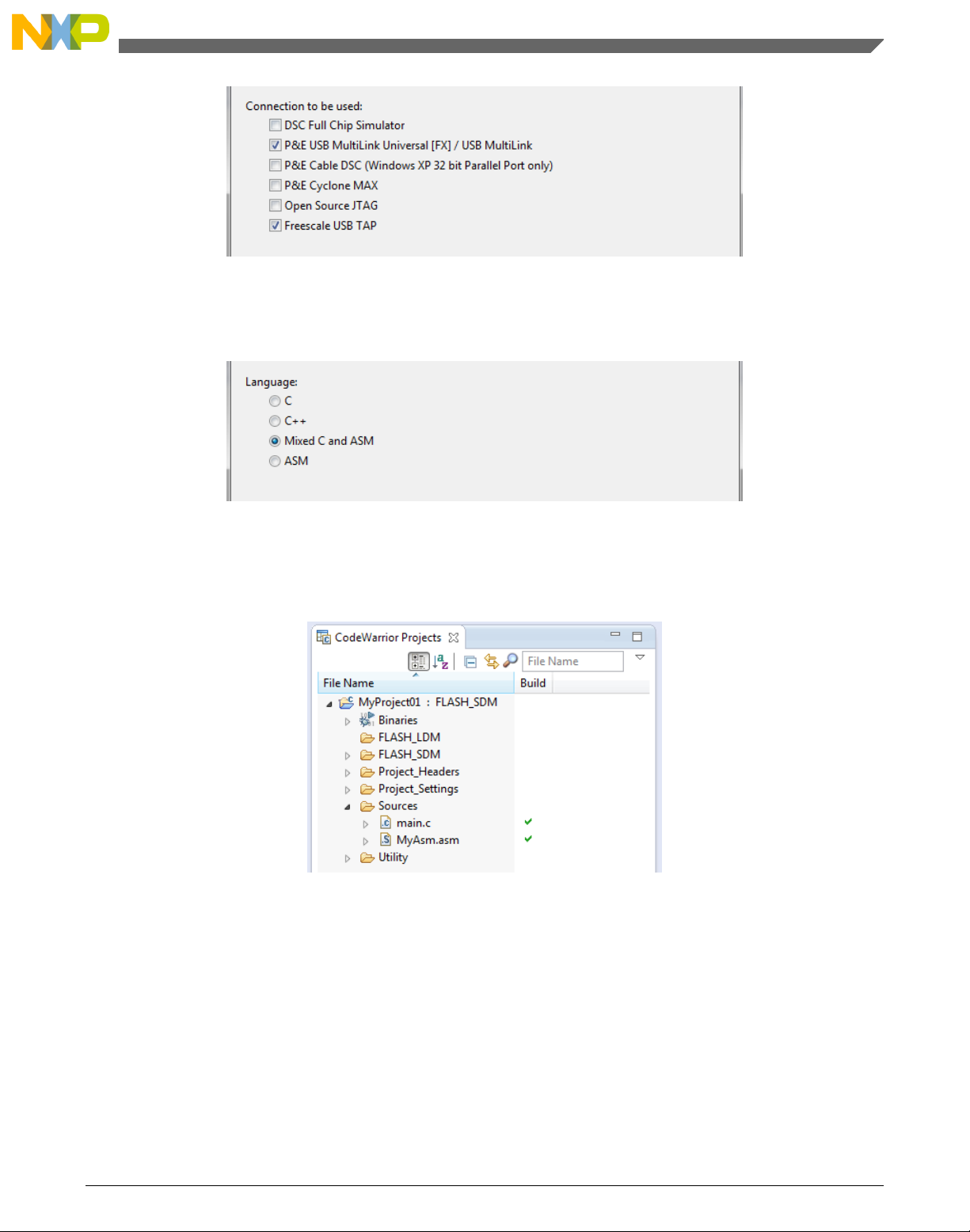
6. Now select the connection that will be used to download and debug the application. In this case, select the option P&E USB MultiLink Universal[FX] / USB MultiLink and Freescale USB TAP, and click Next. See Figure 1-3.

GMCLIB User's Guide, Rev. 2, 10/2015

8 Freescale Semiconductor, Inc.

Chapter 1 Library

Figure 1-3. Connection selection

7. From the options given, select the Simple Mixed Assembly and C language, and click Finish. See Figure 1-4.

Figure 1-4. Language choice

The new project is now visible in the left-hand part of CodeWarrior™ Development Studio. See Figure 1-5.

Figure 1-5. Project folder

1.2.2

Library path variable

To make the library integration easier, create a variable that will hold the information about the library path.

1. Right-click the MyProject01 node in the left-hand part and click Properties, or select Project > Properties from the menu. The project properties dialog appears.

GMCLIB User's Guide, Rev. 2, 10/2015

Freescale Semiconductor, Inc. 9

Library integration into project (CodeWarrior™ Development Studio)

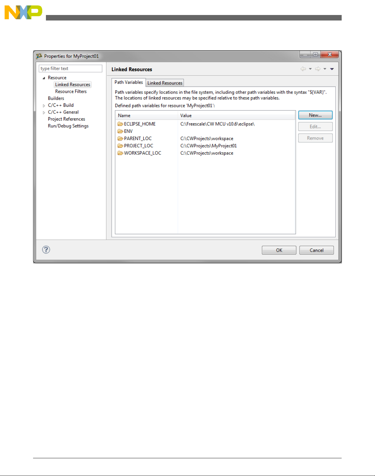
2. Expand the Resource node and click Linked Resources. See Figure 1-6.

Figure 1-6. Project properties

3. Click the 'New…' button on the right-hand side.

4. In the dialog that appears (see Figure 1-7), type this variable name into the Name box: FSLESL_LOC

5. Select the library parent folder by clicking 'Folder…' or just typing the following path into the Location box: C:\Freescale\FSLESL\DSP56800E_FSLESL_4.2_CW and click OK.

6. Click OK in the previous dialog.

GMCLIB User's Guide, Rev. 2, 10/2015

10 Freescale Semiconductor, Inc.

Figure 1-7. New variable

Chapter 1 Library

1.2.3

Library folder addition

To use the library, add it into the CodeWarrior Project tree dialog.

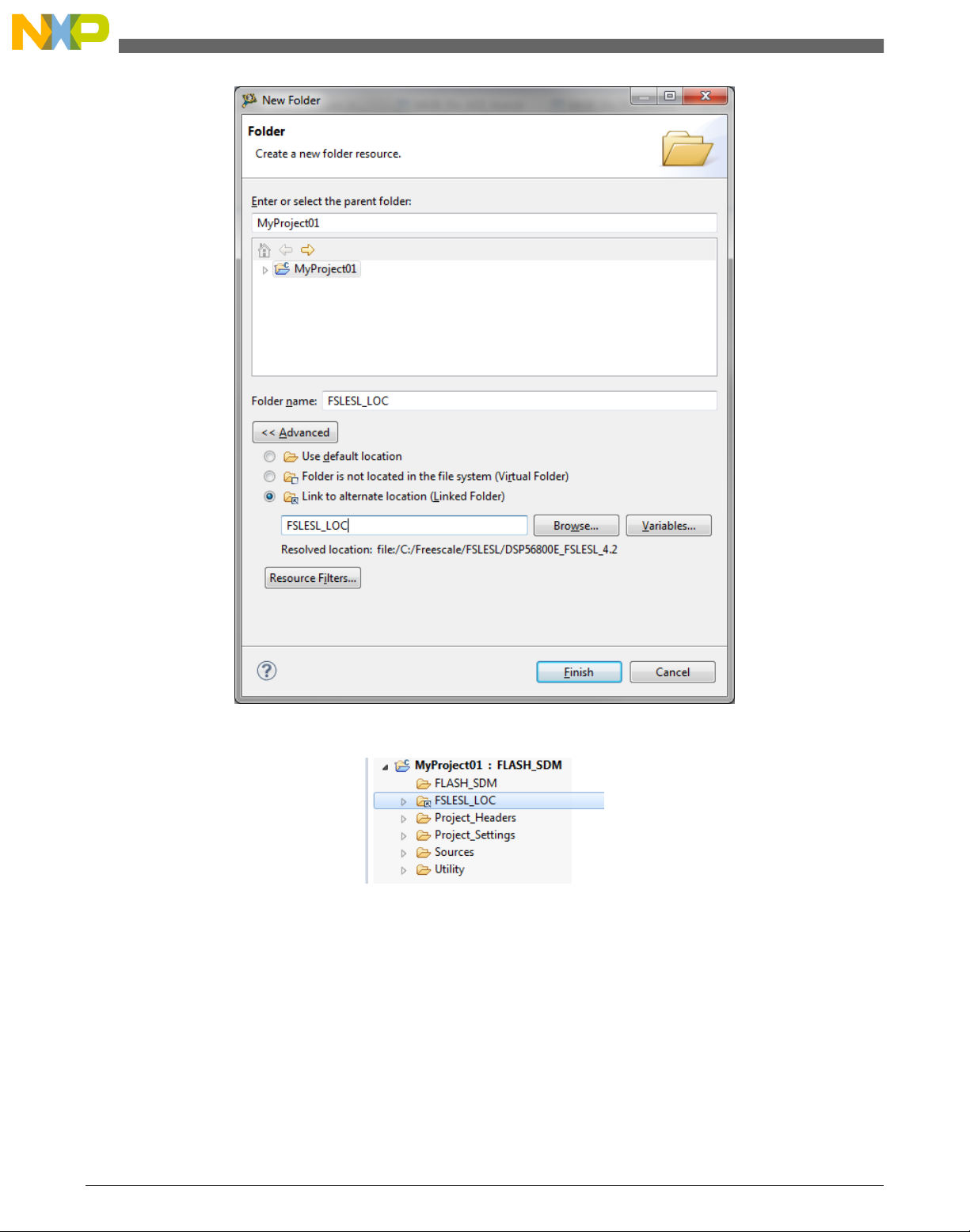
1. Right-click the MyProject01 node in the left-hand part and click New > Folder, or select File > New > Folder from the menu. A dialog appears.

2. Click Advanced to show the advanced options.

3. To link the library source, select the third option—Link to alternate location (Linked Folder).

4. Click Variables…, and select the FSLESL_LOC variable in the dialog that appears, click OK, and/or type the variable name into the box. See Figure 1-8.

5. Click Finish, and you will see the library folder linked in the project. See Figure 1-9

GMCLIB User's Guide, Rev. 2, 10/2015

Freescale Semiconductor, Inc. 11

Library integration into project (CodeWarrior™ Development Studio)

Figure 1-8. Folder link

Figure 1-9. Projects libraries paths

1.2.4

Library path setup

GMCLIB requires MLIB and GFLIB to be included too. Therefore, the following steps show the inclusion of all dependent modules.

1. Right-click the MyProject01 node in the left-hand part and click Properties, or select Project > Properties from the menu. A dialog with the project properties appears.

GMCLIB User's Guide, Rev. 2, 10/2015

12 Freescale Semiconductor, Inc.

Chapter 1 Library

2. Expand the C/C++ Build node, and click Settings.

3. In the right-hand tree, expand the DSC Linker node, and click Input. See Figure 1-11.

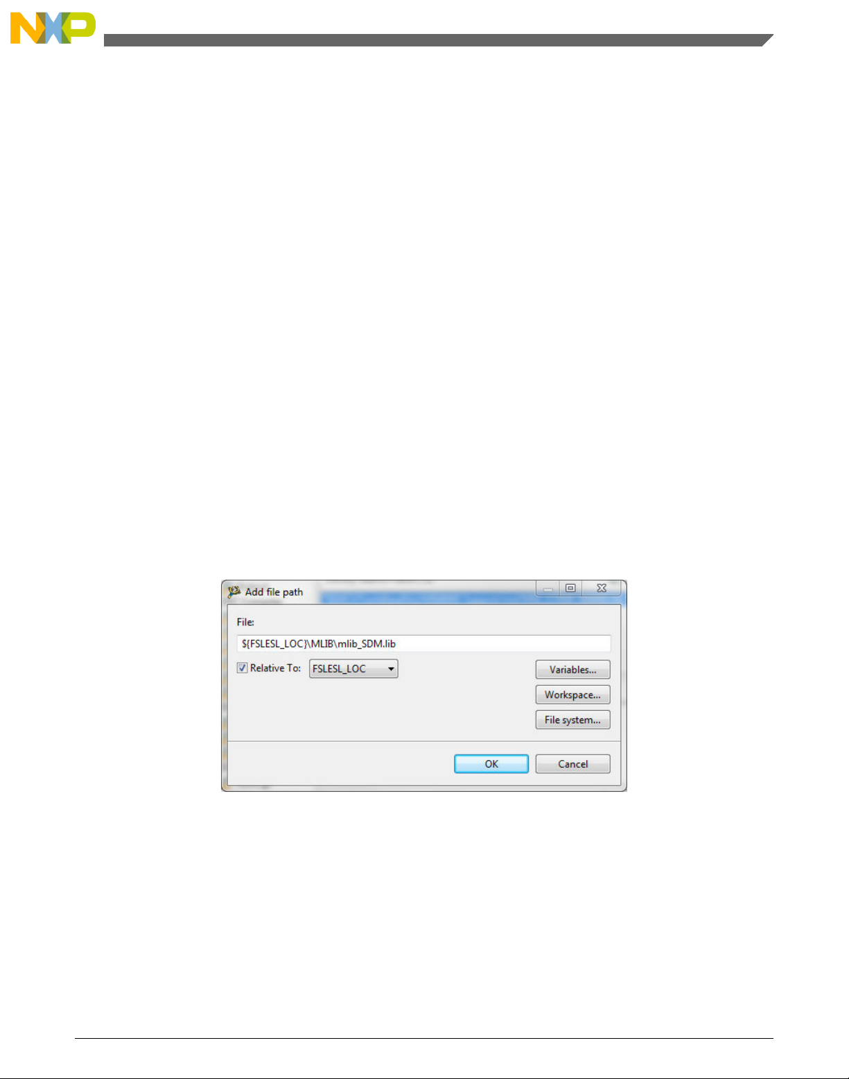
4. In the third dialog Additional Libraries, click the 'Add…' icon, and a dialog appears.

5. Look for the FSLESL_LOC variable by clicking Variables…, and then finish the path in the box by adding one of the following:

• ${FSLESL_LOC}\MLIB\mlib_SDM.lib—for small data model projects

• ${FSLESL_LOC}\MLIB\mlib_LDM.lib—for large data model projects

6. Tick the box Relative To, and select FSLESL_LOC next to the box. See Figure 1-9. Click OK.

7. Click the 'Add…' icon in the third dialog Additional Libraries.

8. Look for the FSLESL_LOC variable by clicking Variables…, and then finish the path in the box by adding one of the following:

• ${FSLESL_LOC}\GFLIB\gflib_SDM.lib—for small data model projects

• ${FSLESL_LOC}\GFLIB\gflib_LDM.lib—for large data model projects

9. Tick the box Relative To, and select FSLESL_LOC next to the box. Click OK.

10. Click the 'Add…' icon in the Additional Libraries dialog.

11. Look for the FSLESL_LOC variable by clicking Variables…, and then finish the path in the box by adding one of the following:

• ${FSLESL_LOC}\GMCLIB\gmclib_SDM.lib—for small data model projects

• ${FSLESL_LOC}\GMCLIB\gmclib_LDM.lib—for large data model projects

12. Tick the box Relative To, and select FSLESL_LOC next to the box. Click OK.

13. Now, you will see the libraries added in the box. See Figure 1-11.

Figure 1-10. Library file inclusion

GMCLIB User's Guide, Rev. 2, 10/2015

Freescale Semiconductor, Inc. 13

Library integration into project (CodeWarrior™ Development Studio)

Figure 1-11. Linker setting

14. In the tree under the DSC Compiler node, click Access Paths.

15. In the Search User Paths dialog (#include “…”), click the 'Add…' icon, and a dialog will appear.

16. Look for the FSLESL_LOC variable by clicking Variables…, and then finish the path in the box to be: ${FSLESL_LOC}\MLIB\include.

17. Tick the box Relative To, and select FSLESL_LOC next to the box. See Figure 1-12. Click OK.

18. Click the 'Add…' icon in the Search User Paths dialog (#include “…”).

19. Look for the FSLESL_LOC variable by clicking Variables…, and then finish the path in the box to be: ${FSLESL_LOC}\GFLIB\include.

20. Tick the box Relative To, and select FSLESL_LOC next to the box. Click OK.

21. Click the 'Add…' icon in the Search User Paths dialog (#include “…”).

22. Look for the FSLESL_LOC variable by clicking Variables…, and then finish the path in the box to be: ${FSLESL_LOC}\GMCLIB\include.

23. Tick the box Relative To, and select FSLESL_LOC next to the box. Click OK.

24. Now you will see the paths added in the box. See Figure 1-13. Click OK.

GMCLIB User's Guide, Rev. 2, 10/2015

14 Freescale Semiconductor, Inc.

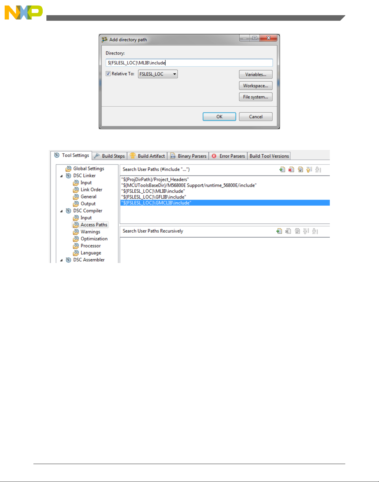
Figure 1-12. Library include path addition

Chapter 1 Library

Figure 1-13. Compiler setting

The final step is typing the #include syntax into the code. Include the library into the main.c file. In the left-hand dialog, open the Sources folder of the project, and doubleclick the main.c file. After the main.c file opens up, include the following lines into the #include section:

#include "mlib.h" #include "gflib.h" #include "gmclib.h"

When you click the Build icon (hammer), the project will be compiled without errors.

GMCLIB User's Guide, Rev. 2, 10/2015

Freescale Semiconductor, Inc. 15

Library integration into project (CodeWarrior™ Development Studio)

GMCLIB User's Guide, Rev. 2, 10/2015

16 Freescale Semiconductor, Inc.

Chapter 2 Algorithms in detail

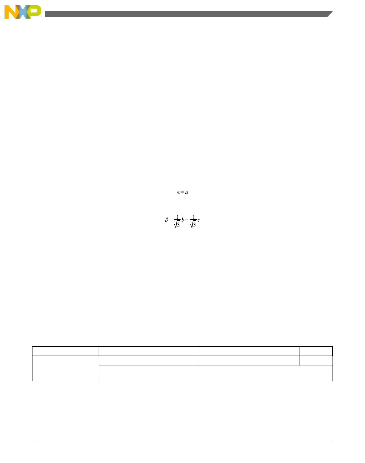
2.1 GMCLIB_Clark

The

GMCLIB_Clark function calculates the Clarke transformation, which is used to

transform values (flux, voltage, current) from the three-phase coordinate system to the two-phase (α-β) orthogonal coordinate system, according to the following equations:

Equation 1

Equation 2

2.1.1

Available versions

This function is available in the following versions:

• Fractional output - the output is the fractional portion of the result; the result is within the range <-1 ; 1). The result may saturate.

The available versions of the GMCLIB_Clark function are shown in the following table:

Table 2-1. Function versions

Function name Input type Output type Result type

GMCLIB_Clark_F16 GMCLIB_3COOR_T_F16 * GMCLIB_2COOR_ALBE_T_F16 * void

Clarke transformation of a 16-bit fractional three-phase system input to a 16-bit fractional twophase system. The input and output are within the fractional range <-1 ; 1).

GMCLIB User's Guide, Rev. 2, 10/2015

Freescale Semiconductor, Inc. 17

GMCLIB_ClarkInv

2.1.2 Declaration

The available GMCLIB_Clark functions have the following declarations:

void GMCLIB_Clark_F16(const GMCLIB_3COOR_T_F16 *psIn, GMCLIB_2COOR_ALBE_T_F16 *psOut)

2.1.3 Function use

The use of the GMCLIB_Clark function is shown in the following example:

#include "gmclib.h"

static GMCLIB_2COOR_ALBE_T_F16 sAlphaBeta; static GMCLIB_3COOR_T_F16 sAbc;

void Isr(void);

void main(void) { /* ABC structure initialization */ sAbc.f16A = FRAC16(0.0); sAbc.f16B = FRAC16(0.0); sAbc.f16C = FRAC16(0.0); }

/* Periodical function or interrupt */ void Isr(void) { /* Clarke Transformation calculation */ GMCLIB_Clark_F16(&sAbc, &sAlphaBeta); }

2.2

GMCLIB_ClarkInv

The GMCLIB_ClarkInv function calculates the Clarke transformation, which is used to transform values (flux, voltage, current) from the two-phase (α-β) orthogonal coordinate system to the three-phase coordinate system, according to the following equations:

Equation 3

Equation 4

Equation 5

GMCLIB User's Guide, Rev. 2, 10/2015

18 Freescale Semiconductor, Inc.

Chapter 2 Algorithms in detail

2.2.1 Available versions

This function is available in the following versions:

• Fractional output - the output is the fractional portion of the result; the result is within the range <-1 ; 1). The result may saturate.

The available versions of the GMCLIB_ClarkInv function are shown in the following table:

Table 2-2. Function versions

Function name Input type Output type Result type

GMCLIB_ClarkInv_F16 GMCLIB_2COOR_ALBE_T_F16 * GMCLIB_3COOR_T_F16 * void

Inverse Clarke transformation with a 16-bit fractional two-phase system input and a 16-bit fractional three-phase output. The input and output are within the fractional range <-1 ; 1).

2.2.2 Declaration

The available GMCLIB_ClarkInv functions have the following declarations:

void GMCLIB_ClarkInv_F16(const GMCLIB_2COOR_ALBE_T_F16 *psIn, GMCLIB_3COOR_T_F16 *psOut)

2.2.3

The use of the GMCLIB_ClarkInv function is shown in the following example:

#include "gmclib.h"

static GMCLIB_2COOR_ALBE_T_F16 sAlphaBeta; static GMCLIB_3COOR_T_F16 sAbc;

void Isr(void);

void main(void) { /* Alpha, Beta structure initialization */ sAlphaBeta.f16Alpha = FRAC16(0.0); sAlphaBeta.f16Beta = FRAC16(0.0); }

Function use

/* Periodical function or interrupt */ void Isr(void) { /* Inverse Clarke Transformation calculation */ GMCLIB_ClarkInv_F16(&sAlphaBeta, &sAbc); }

GMCLIB User's Guide, Rev. 2, 10/2015

Freescale Semiconductor, Inc. 19

GMCLIB_Park

2.3 GMCLIB_Park

The GMCLIB_Park function calculates the Park transformation, which transforms values (flux, voltage, current) from the stationary two-phase (α-β) orthogonal coordinate system to the rotating two-phase (d-q) orthogonal coordinate system, according to the following equations:

Equation 6

Equation 7

where:

• θ is the position (angle)

2.3.1

Available versions

This function is available in the following versions:

• Fractional output - the output is the fractional portion of the result; the result is within the range <-1 ; 1). The result may saturate.

The available versions of the GMCLIB_Park function are shown in the following table:

Table 2-3. Function versions

Function name Input type Output type Result type

GMCLIB_Park_F16 GMCLIB_2COOR_ALBE_T_F16 * GMCLIB_2COOR_DQ_T_F16 * void

GMCLIB_2COOR_SINCOS_T_F16 *

The Park transformation of a 16-bit fractional two-phase stationary system input to a 16-bit fractional two-phase rotating system, using a 16-bit fractional angle two-component (sin / cos) position information. The inputs and the output are within the fractional range <-1 ; 1).

2.3.2 Declaration

The available GMCLIB_Park functions have the following declarations:

void GMCLIB_Park_F16(const GMCLIB_2COOR_ALBE_T_F16 *psIn, const GMCLIB_2COOR_SINCOS_T_F16 *psAnglePos, GMCLIB_2COOR_DQ_T_F16 *psOut)

GMCLIB User's Guide, Rev. 2, 10/2015

20 Freescale Semiconductor, Inc.

Chapter 2 Algorithms in detail

2.3.3 Function use

The use of the GMCLIB_Park function is shown in the following example:

#include "gmclib.h"

static GMCLIB_2COOR_ALBE_T_F16 sAlphaBeta; static GMCLIB_2COOR_DQ_T_F16 sDQ; static GMCLIB_2COOR_SINCOS_T_F16 sAngle;

void Isr(void);

void main(void) { /* Alpha, Beta structure initialization */ sAlphaBeta.f16Alpha = FRAC16(0.0); sAlphaBeta.f16Beta = FRAC16(0.0);

/* Angle structure initialization */ sAngle.f16Sin = FRAC16(0.0); sAngle.f16Cos = FRAC16(1.0); }

/* Periodical function or interrupt */ void Isr(void) { /* Park Transformation calculation */ GMCLIB_Park_F16(&sAlphaBeta, &sAngle, &sDQ); }

2.4

GMCLIB_ParkInv

The GMCLIB_ParkInv function calculates the Park transformation, which transforms values (flux, voltage, current) from the rotating two-phase (d-q) orthogonal coordinate system to the stationary two-phase (α-β) coordinate system, according to the following equations:

Equation 8

Equation 9

where:

• θ is the position (angle)

GMCLIB User's Guide, Rev. 2, 10/2015

Freescale Semiconductor, Inc. 21

GMCLIB_ParkInv

2.4.1 Available versions

This function is available in the following versions:

• Fractional output - the output is the fractional portion of the result; the result is within the range <-1 ; 1). The result may saturate.

The available versions of the GMCLIB_ParkInv function are shown in the following table:

Table 2-4. Function versions

Function name Input type Output type Result type

GMCLIB_ParkInv_F16 GMCLIB_2COOR_DQ_T_F16 * GMCLIB_2COOR_ALBE_T_F16 * void

GMCLIB_2COOR_SINCOS_T_F16 *

Inverse Park transformation of a 16-bit fractional two-phase rotating system input to a 16-bit fractional two-phase stationary system, using a 16-bit fractional angle two-component (sin / cos) position information. The inputs and the output are within the fractional range <-1 ; 1).

2.4.2 Declaration

The available GMCLIB_ParkInv functions have the following declarations:

void GMCLIB_ParkInv_F16(const GMCLIB_2COOR_DQ_T_F16 *psIn, const GMCLIB_2COOR_SINCOS_T_F16 *psAnglePos, GMCLIB_2COOR_ALBE_T_F16 *psOut)

2.4.3

The use of the GMCLIB_ParkInv function is shown in the following example:

#include "gmclib.h"

static GMCLIB_2COOR_ALBE_T_F16 sAlphaBeta; static GMCLIB_2COOR_DQ_T_F16 sDQ; static GMCLIB_2COOR_SINCOS_T_F16 sAngle;

void Isr(void);

void main(void) { /* D, Q structure initialization */ sDQ.f16D = FRAC16(0.0); sDQ.f16Q = FRAC16(0.0);

/* Angle structure initialization */ sAngle.f16Sin = FRAC16(0.0); sAngle.f16Cos = FRAC16(1.0); }

Function use

/* Periodical function or interrupt */

GMCLIB User's Guide, Rev. 2, 10/2015

22 Freescale Semiconductor, Inc.

Chapter 2 Algorithms in detail

void Isr(void) { /* Inverse Park Transformation calculation */ GMCLIB_ParkInv_F16(&sDQ, &sAngle, &sAlphaBeta); }

2.5 GMCLIB_DecouplingPMSM

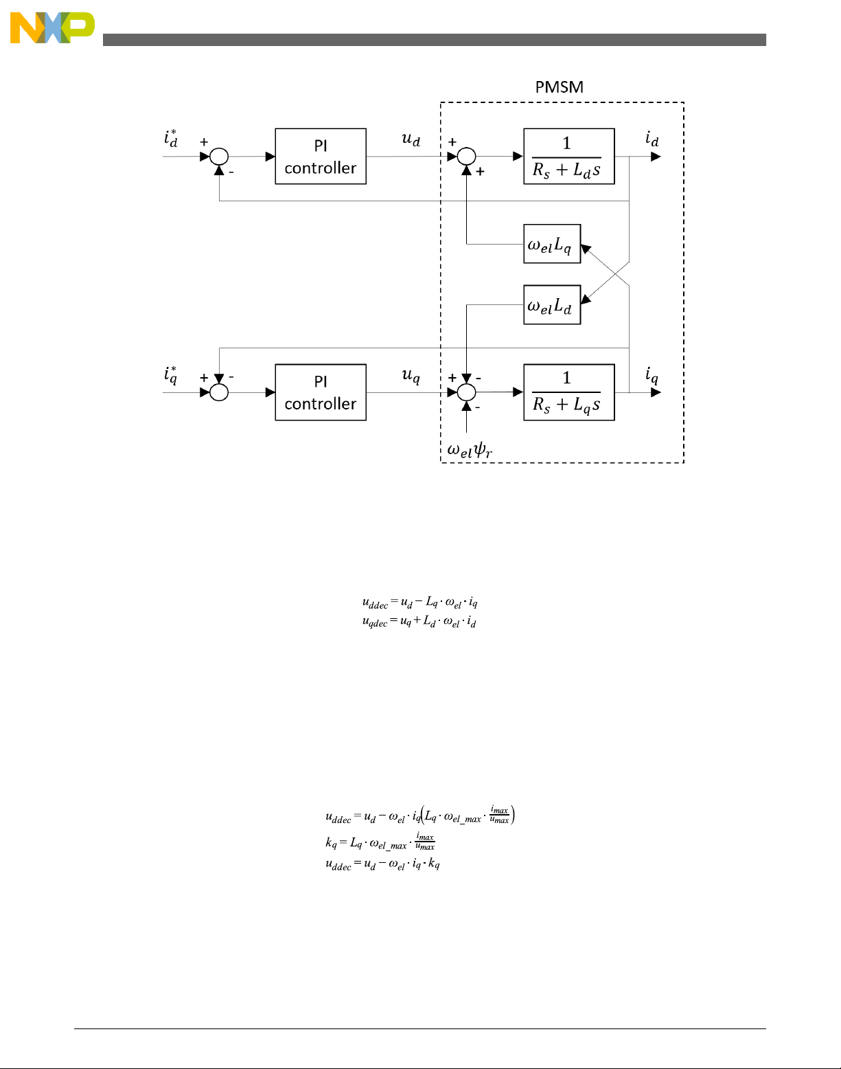
The GMCLIB_DecouplingPMSM function calculates the cross-coupling voltages to eliminate the d-q axis coupling that causes nonlinearity of the control.

The d-q model of the motor contains cross-coupling voltage that causes nonlinearity of the control. Figure 2-1 represents the d-q model of the motor that can be described using the following equations, where the underlined portion is the cross-coupling voltage:

Equation 10

where:

• ud, uq are the d and q voltages

• id, iq are the d and q currents

• Rs is the stator winding resistance

• Ld, Lq are the stator winding d and q inductances

• ωel is the electrical angular speed

• ψr is the rotor flux constant

GMCLIB User's Guide, Rev. 2, 10/2015

Freescale Semiconductor, Inc. 23

GMCLIB_DecouplingPMSM

Figure 2-1. The d-q PMSM model

To eliminate the nonlinearity, the cross-coupling voltage is calculated using the

GMCLIB_DecouplingPMSM algorithm, and feedforwarded to the d and q voltages. The

decoupling algorithm is calculated using the following equations:

Equation 11

where:

• ud, uq are the d and q voltages; inputs to the algorithm

• u

ddec

, u

are the d and q decoupled voltages; outputs from the algorithm

qdec

The fractional representation of the d-component equation is as follows:

Equation 12

The fractional representation of the q-component equation is as follows:

GMCLIB User's Guide, Rev. 2, 10/2015

24 Freescale Semiconductor, Inc.

Equation 13

where:

• kd, kq are the scaling coefficients

• i

• u

• ω

is the maximum current

max

is the maximum voltage

max

el_max

is the maximum electrical speed

The kd and kq parameters must be set up properly. The principle of the algorithm is depicted in Figure 2-2 :

Chapter 2 Algorithms in detail

Figure 2-2. Algorithm diagram

2.5.1

Available versions

This function is available in the following versions:

• Fractional output - the output is the fractional portion of the result; the result is within the range <-1 ; 1). The result may saturate. The parameters use the accumulator types.

GMCLIB User's Guide, Rev. 2, 10/2015

Freescale Semiconductor, Inc. 25

GMCLIB_DecouplingPMSM

The available versions of the GMCLIB_DecouplingPMSM function are shown in the following table:

Table 2-5. Function versions

Function name Input/output type Result type

GMCLIB_DecouplingPMSM_F16

Input

Parameters Output

The PMSM decoupling with a 16-bit fractional d-q voltage, current inputs, and a 16bit fractional electrical speed input. The parameters are 32-bit accumulator types. The output is a 16-bit fractional decoupled d-q voltage. The inputs and the output are within the range <-1 ; 1).

GMCLIB_2COOR_DQ_T_F16 * void GMCLIB_2COOR_DQ_T_F16 * frac16_t GMCLIB_DECOUPLINGPMSM_T_A32 * GMCLIB_2COOR_DQ_T_F16 *

2.5.2 GMCLIB_DECOUPLINGPMSM_T_A32 type description

Variable name Input type Description

a32KdGain acc32_t Direct axis decoupling parameter. The parameter is within the range <0 ; 65536.0) a32KqGain acc32_t Quadrature axis decoupling parameter. The parameter is within the range <0 ;

65536.0)

2.5.3 Declaration

The available GMCLIB_DecouplingPMSM functions have the following declarations:

void GMCLIB_DecouplingPMSM_F16(const GMCLIB_2COOR_DQ_T_F16 *psUDQ, const

GMCLIB_2COOR_DQ_T_F16 *psIDQ, frac16_t f16SpeedEl, const GMCLIB_DECOUPLINGPMSM_T_A32

*psParam, GMCLIB_2COOR_DQ_T_F16 *psUDQDec)

2.5.4

The use of the GMCLIB_DecouplingPMSM function is shown in the following example:

Function use

#include "gmclib.h"

static GMCLIB_2COOR_DQ_T_F16 sVoltageDQ; static GMCLIB_2COOR_DQ_T_F16 sCurrentDQ; static frac16_t f16AngularSpeed; static GMCLIB_DECOUPLINGPMSM_T_A32 sDecouplingParam; static GMCLIB_2COOR_DQ_T_F16 sVoltageDQDecoupled;

GMCLIB User's Guide, Rev. 2, 10/2015

26 Freescale Semiconductor, Inc.

Chapter 2 Algorithms in detail

void Isr(void);

void main(void) { /* Voltage D, Q structure initialization */ sVoltageDQ.f16D = FRAC16(0.0); sVoltageDQ.f16Q = FRAC16(0.0);

/* Current D, Q structure initialization */ sCurrentDQ.f16D = FRAC16(0.0); sCurrentDQ.f16Q = FRAC16(0.0);

/* Speed initialization */ f16AngularSpeed = FRAC16(0.0);

/* Motor parameters for decoupling Kd = 40, Kq = 20 */ sDecouplingParam.a32KdGain = ACC32(40.0); sDecouplingParam.a32KqGain = ACC32(20.0); }

/* Periodical function or interrupt */ void Isr(void) { /* Decoupling calculation */ GMCLIB_DecouplingPMSM_F16(&sVoltageDQ, &sCurrentDQ, f16AngularSpeed, &sDecouplingParam, &sVoltageDQDecoupled); }

2.6

GMCLIB_ElimDcBusRipFOC

The GMCLIB_ElimDcBusRipFOC function is used for the correct PWM duty cycle output calculation, based on the measured DC-bus voltage. The side effect is the elimination of the the DC-bus voltage ripple in the output PWM duty cycle. This function is meant to be used with a space vector modulation, whose modulation index (with respect to the DC-bus voltage) is an inverse square root of 3.

The general equation to calculate the duty cycle for the above-mentioned space vector modulation is as follows:

Equation 14

where:

• U

• u

is the duty cycle output

PWM

is the real FOC voltage

FOC

is the real measured DC-bus voltage

dcbus

Using the previous equations, the GMCLIB_ElimDcBusRipFOC function compensates an amplitude of the direct-α and the quadrature-β component of the stator-reference voltage vector, using the formula shown in the following equations:

GMCLIB User's Guide, Rev. 2, 10/2015

Freescale Semiconductor, Inc. 27

GMCLIB_ElimDcBusRipFOC

where:

• Uα* is the direct-α duty cycle ratio

• Uβ* is the direct-β duty cycle ratio

• Uα is the direct-α voltage

• Uβ is the quadrature-β voltage

Equation 15

Equation 16

If the fractional arithmetic is used, the FOC and DC-bus voltages have their scales, which take place in Equation 14 on page 27; the equation is as follows:

Equation 17

where:

• U

is the scaled FOC voltage

FOC

is the scaled measured DC-bus voltage

dcbus FOC_max dcbus_max

is the FOC voltage scale

is the DC-bus voltage scale

If this algorithm is used with the space vector modulation with the ratio of square root equal to 3, then the FOC voltage scale is expressed as follows :

Equation 18

The equation can be simplified as follows:

GMCLIB User's Guide, Rev. 2, 10/2015

28 Freescale Semiconductor, Inc.

Chapter 2 Algorithms in detail

Equation 19

The GMCLIB_ElimDcBusRipFOC function compensates an amplitude of the direct-α and the quadrature-β component of the stator-reference voltage vector in the fractional arithmetic, using the formula shown in the following equations:

Equation 20

Equation 21

where:

• Uα* is the direct-α duty cycle ratio

• Uβ* is the direct-β duty cycle ratio

• Uα is the direct-α voltage

• Uβ is the quadrature-β voltage

The GMCLIB_ElimDcBusRipFOC function can be used in general motor-control applications, and it provides elimination of the voltage ripple on the DC-bus of the power stage. Figure 2-3 shows the results of the DC-bus ripple elimination, while compensating the ripples of the rectified voltage using a three-phase uncontrolled rectifier.

GMCLIB User's Guide, Rev. 2, 10/2015

Freescale Semiconductor, Inc. 29

GMCLIB_ElimDcBusRipFOC

Figure 2-3. Results of the DC-bus voltage ripple elimination

2.6.1

Available versions

This function is available in the following versions:

• Fractional output - the output is the fractional portion of the result; the result is within the range <-1 ; 1). The result may saturate.

The available versions of the GMCLIB_ElimDcBusRipFOC function are shown in the following table:

Table 2-6. Function versions

Function name Input type Output type Result

type

GMCLIB_ElimDcBusRipFOC_F16 frac16_t GMCLIB_2COOR_ALBE_T_F16 * void

GMCLIB_2COOR_ALBE_T_F16 *

Table continues on the next page...

GMCLIB User's Guide, Rev. 2, 10/2015

30 Freescale Semiconductor, Inc.

Chapter 2 Algorithms in detail

Table 2-6. Function versions (continued)

Function name Input type Output type Result

type

Compensation of a 16-bit fractional two-phase system input to a 16-bit fractional two-phase system, using a 16-bit fractional DC-bus voltage information. The DCbus voltage input is within the fractional range <0 ; 1); the stationary (α-β) voltage input and the output are within the fractional range <-1 ; 1).

2.6.2 Declaration

The available GMCLIB_ElimDcBusRipFOC functions have the following declarations:

void GMCLIB_ElimDcBusRipFOC_F16(frac16_t f16UDCBus, const GMCLIB_2COOR_ALBE_T_F16 *psUAlBe,

GMCLIB_2COOR_ALBE_T_F16 *psUAlBeComp)

2.6.3

Function use

The use of the GMCLIB_ElimDcBusRipFOC function is shown in the following example:

#include "gmclib.h"

static frac16_t f16UDcBus; static GMCLIB_2COOR_ALBE_T_F16 sUAlBe; static GMCLIB_2COOR_ALBE_T_F16 sUAlBeComp;

void Isr(void);

void main(void) { /* Voltage Alpha, Beta structure initialization */ sUAlBe.f16Alpha = FRAC16(0.0); sUAlBe.f16Beta = FRAC16(0.0);

/* DC bus voltage initialization */ f16DcBus = FRAC16(0.8); }

/* Periodical function or interrupt */ void Isr(void) { /* FOC Ripple elimination calculation */ GMCLIB_ElimDcBusRipFOC_F16(f16UDcBus, &sUAlBe, &sUAlBeComp); }

2.7

Freescale Semiconductor, Inc. 31

GMCLIB_ElimDcBusRip

GMCLIB User's Guide, Rev. 2, 10/2015

GMCLIB_ElimDcBusRip

The GMCLIB_ElimDcBusRip function is used for a correct PWM duty cycle output calculation, based on the measured DC-bus voltage. The side effect is the elimination of the the DC-bus voltage ripple in the output PWM duty cycle. This function can be used with any kind of space vector modulation; it has an additional input - the modulation index (with respect to the DC-bus voltage).

The general equation to calculate the duty cycle is as follows:

Equation 22

where:

• U

• u

• i

mod

is the duty cycle output

PWM

is the real FOC voltage

FOC

is the real measured DC-bus voltage

dcbus

is the space vector modulation index

Using the previous equations, the GMCLIB_ElimDcBusRip function compensates an amplitude of the direct-α and the quadrature-β component of the stator-reference voltage vector, using the formula shown in the following equations:

Equation 23

Equation 24

where:

• Uα* is the direct-α duty cycle ratio

• Uβ* is the direct-β duty cycle ratio

• Uα is the direct-α voltage

• Uβ is the quadrature-β voltage

If the fractional arithmetic is used, the FOC and DC-bus voltages have their scales, which take place in Equation 22 on page 32; the equation is as follows:

GMCLIB User's Guide, Rev. 2, 10/2015

32 Freescale Semiconductor, Inc.

where:

Chapter 2 Algorithms in detail

Equation 25

• U

is the scaled FOC voltage

FOC

is the scaled measured DC-bus voltage

dcbus FOC_max dcbus_max

is the FOC voltage scale

is the DC-bus voltage scale

Thus, the modulation index in the fractional representation is expressed as follows :

Equation 26

where:

• i

is the space vector modulation index in the fractional arithmetic

modfr

The GMCLIB_ElimDcBusRip function compensates an amplitude of the direct-α and the quadrature-β component of the stator-reference voltage vector in the fractional arithmetic, using the formula shown in the following equations:

Equation 27

Equation 28

where:

• Uα* is the direct-α duty cycle ratio

• Uβ* is the direct-β duty cycle ratio

• Uα is the direct-α voltage

• Uβ is the quadrature-β voltage

GMCLIB User's Guide, Rev. 2, 10/2015

Freescale Semiconductor, Inc. 33

GMCLIB_ElimDcBusRip

The GMCLIB_ElimDcBusRip function can be used in general motor-control applications, and it provides elimination of the voltage ripple on the DC-bus of the power stage. Figure 2-4 shows the results of the DC-bus ripple elimination, while compensating the ripples of the rectified voltage, using a three-phase uncontrolled rectifier.

Figure 2-4. Results of the DC-bus voltage ripple elimination

2.7.1

Available versions

This function is available in the following versions:

• Fractional output - the output is the fractional portion of the result; the result is within the range <-1 ; 1). The result may saturate. The modulation index is a nonnegative accumulator type value.

GMCLIB User's Guide, Rev. 2, 10/2015

34 Freescale Semiconductor, Inc.

Chapter 2 Algorithms in detail

The available versions of the GMCLIB_ElimDcBusRip function are shown in the following table:

Table 2-7. Function versions

Function name Input type Output type Result

GMCLIB_ElimDcBusRip_F16sas frac16_t GMCLIB_2COOR_ALBE_T_F16 * void

acc32_t GMCLIB_2COOR_ALBE_T_F16 *

Compensation of a 16-bit fractional two-phase system input to a 16-bit fractional two-phase system using a 16-bit fractional DC-bus voltage information and a 32-bit accumulator modulation index. The DC-bus voltage input is within the fractional range <0 ; 1); the modulation index is a non-negative value; the stationary (α-β) voltage input and output are within the fractional range <-1 ; 1).

2.7.2 Declaration

type

The available GMCLIB_ElimDcBusRip functions have the following declarations:

void GMCLIB_ElimDcBusRip_F16sas(frac16_t f16UDCBus, acc32_t a32IdxMod, const

GMCLIB_2COOR_ALBE_T_F16 *psUAlBeComp, GMCLIB_2COOR_ALBE_T_F16 *psUAlBe)

2.7.3

Function use

The use of the GMCLIB_ElimDcBusRip function is shown in the following example:

#include "gmclib.h"

static frac16_t f16UDcBus; static acc32_t a32IdxMod; static GMCLIB_2COOR_ALBE_T_F16 sUAlBe; static GMCLIB_2COOR_ALBE_T_F16 sUAlBeComp;

void Isr(void);

void main(void) { /* Voltage Alpha, Beta structure initialization */ sUAlBe.f16Alpha = FRAC16(0.0); sUAlBe.f16Beta = FRAC16(0.0);

/* SVM modulation index */ a32IdxMod = ACC32(1.3);

/* DC bus voltage initialization */ f16UDcBus = FRAC16(0.8); }

/* Periodical function or interrupt */ void Isr(void)

GMCLIB User's Guide, Rev. 2, 10/2015

Freescale Semiconductor, Inc. 35

GMCLIB_SvmStd

{ /* Ripple elimination calculation */ GMCLIB_ElimDcBusRip_F16sas(f16UDcBus, a32IdxMod, &sUAlBe, &sUAlBeComp); }

2.8 GMCLIB_SvmStd

The GMCLIB_SvmStd function calculates the appropriate duty-cycle ratios, which are needed for generation of the given stator-reference voltage vector, using a special standard space vector modulation technique.

The GMCLIB_SvmStd function for calculating the duty-cycle ratios is widely used in modern electric drives. This function calculates the appropriate duty-cycle ratios, which are needed for generating the given stator reference voltage vector, using a special space vector modulation technique, called standard space vector modulation.

The basic principle of the standard space vector modulation technique can be explained using the power stage diagram shown in Figure 2-5.

Figure 2-5. Power stage schematic diagram

GMCLIB User's Guide, Rev. 2, 10/2015

36 Freescale Semiconductor, Inc.

Chapter 2 Algorithms in detail

The top and bottom switches are working in a complementary mode; for example, if the top switch SAt is on, then the corresponding bottom switch SAb is off, and vice versa. Considering that the value 1 is assigned to the ON state of the top switch, and value 0 is assigned to the ON state of the bottom switch, the switching vector [a, b, c]T can be defined. Creating of such vector allows for numerical definition of all possible switching states. Phase-to-phase voltages can then be expressed in terms of the following states:

Equation 29

where U

DCBus

is the instantaneous voltage measured on the DC-bus.

Assuming that the motor is completely symmetrical, it is possible to write a matrix equation, which expresses the motor phase voltages shown in Equation 29 on page 37.

Equation 30

In a three-phase power stage configuration (as shown in Figure 2-5), eight possible switching states (shown in Figure 2-6) are feasible. These states, together with the resulting instantaneous output line-to-line and phase voltages, are listed in Table 2-8.

Table 2-8. Switching patterns

A B C U

0 0 0 0 0 0 0 0 0 O 1 0 0 2U 1 1 0 U 0 1 0 -U 0 1 1 -2U 0 0 1 -U 1 0 1 U

/3 -U

DCBus

/3 U

DCBus

/3 2U

DCBus

/3 U

DCBus

/3 -U

DCBus

/3 -2U

DCBus

1 1 1 0 0 0 0 0 0 O

/3 -U

DCBus

/3 -2U

DCBus

/3 -U

DCBus

/3 U

DCBus

/3 2U

DCBus

/3 U

DCBus

/3 U

DCBus

/3 0 U

DCBus

/3 -U

DCBus

/3 -U

DCBus

/3 0 -U

DCBus

/3 U

DCBus

0 -U

DCBus

0 U

DCBus

-U

DCBus

-U

DCBus

0 U

DCBus

0 U

Vector

000

120

240

300

360

111

The quantities of the direct-α and the quadrature-β components of the two-phase orthogonal coordinate system, describing the three-phase stator voltages, are expressed using the Clark transformation, arranged in a matrix form:

GMCLIB User's Guide, Rev. 2, 10/2015

Freescale Semiconductor, Inc. 37

GMCLIB_SvmStd

Equation 31

The three-phase stator voltages - Ua, Ub, and Uc, are transformed using the Clark transformation into the direct-α and the quadrature-β components of the two-phase orthogonal coordinate system. The transformation results are listed in Table 2-9.

Table 2-9. Switching patterns and space vectors

A B C U

0 0 0 0 0 O 1 0 0 2U 1 1 0 U 0 1 0 -U 0 1 1 -2U 0 0 1 -U 1 0 1 U 1 1 1 0 0 O

/3 0 U

DCBus

/3 U

DCBus

/3 U

DCBus

/3 0 U

DCBus

/3 -U

DCBus

/3 -U

DCBus

/√3 U

DCBus

/√3 U

DCBus

/√3 U

DCBus

/√3 U

DCBus

Vector

000

120

240

300

360

111

Figure 2-6 depicts the basic feasible switching states (vectors). There are six nonzero

vectors - U0, U60,U

120

, U

180

, U

, and U

240

, and two zero vectors - O

300

111

and O

, usable

000

for switching. Therefore, the principle of the standard space vector modulation lies in applying the appropriate switching states for a certain time, and thus generating a voltage vector identical to the reference one.

GMCLIB User's Guide, Rev. 2, 10/2015

38 Freescale Semiconductor, Inc.

Chapter 2 Algorithms in detail

Figure 2-6. Basic space vectors

Referring to this principle, the objective of the standard space vector modulation is an approximation of the reference stator voltage vector US, with an appropriate combination of the switching patterns, composed of basic space vectors. The graphical explanation of this objective is shown in Figure 2-7 and Figure 2-8.

GMCLIB User's Guide, Rev. 2, 10/2015

Freescale Semiconductor, Inc. 39

GMCLIB_SvmStd

Figure 2-7. Projection of reference voltage vector in the respective sector

The stator reference voltage vector US is phase-advanced by 30° from the direct-α, and thus can be generated with an appropriate combination of the adjacent basic switching states U0 and U60. These figures also indicate the resultant direct-α and quadrature-β components for space vectors U0 and U60.

GMCLIB User's Guide, Rev. 2, 10/2015

40 Freescale Semiconductor, Inc.

Chapter 2 Algorithms in detail

Figure 2-8. Detail of the voltage vector projection in the respective sector

In this case, the reference stator voltage vector US is located in sector I, and can be generated using the appropriate duty-cycle ratios of the basic switching states U0 and U60. The principal equations concerning this vector location are as follows:

Equation 32

where T60 and T0 are the respective duty-cycle ratios, for which the basic space vectors T60 and T0 should be applied within the time period T. T vectors O

000

and O

are applied. Those duty-cycle ratios can be calculated using the

111

is the time, for which the null

null

following equations:

GMCLIB User's Guide, Rev. 2, 10/2015

Freescale Semiconductor, Inc. 41

GMCLIB_SvmStd

Equation 33

Considering that normalized magnitudes of basic space vectors are |U60| = |U0| = 2 / √3, and by the substitution of the trigonometric expressions sin 60° and tan 60° by their quantities 2 / √3, and √3, respectively, the Equation 33 on page 42 can be rearranged for the unknown duty-cycle ratios T60 / T and T0 / T as follows:

Equation 34

Sector II is depicted in Figure 2-9. In this particular case, the reference stator voltage vector US is generated using the appropriate duty-cycle ratios of the basic switching states T60 and T

. The basic equations describing this sector are as follows:

120

Equation 35

where T U

and U60 should be applied within the time period T. T

120

null vectors O

and T60 are the respective duty-cycle ratios, for which the basic space vectors

120

is the time, for which the

null

000

and O

are applied. These resultant duty-cycle ratios are formed from

111

the auxiliary components, termed A and B. The graphical representation of the auxiliary components is shown in Figure 2-10.

GMCLIB User's Guide, Rev. 2, 10/2015

42 Freescale Semiconductor, Inc.

Chapter 2 Algorithms in detail

Figure 2-9. Projection of the reference voltage vector in the respective sector

GMCLIB User's Guide, Rev. 2, 10/2015

Freescale Semiconductor, Inc. 43

GMCLIB_SvmStd

Figure 2-10. Detail of the voltage vector projection in the respective sector

The equations describing those auxiliary time-duration components are as follows:

Equation 36

Equations in Equation 36 on page 44 have been created using the sine rule. The resultant duty-cycle ratios T

/ T and T60 / T are then expressed in terms of the

120

auxiliary time-duration components, defined by Equation 37 on page 44 as follows:

Equation 37

GMCLIB User's Guide, Rev. 2, 10/2015

44 Freescale Semiconductor, Inc.

Chapter 2 Algorithms in detail

Using these equations, and also considering that the normalized magnitudes of the basic space vectors are |U cycle ratios of basic space vectors T

| = |U60| = 2 / √3 , the equations expressed for the unknown duty-

120

/ T and T60 / T can be expressed as follows:

120

Equation 38

The duty-cycle ratios in the remaining sectors can be derived using the same approach. The resulting equations will be similar to those derived for sector I and sector II.

Equation 39

To depict the duty-cycle ratios of the basic space vectors for all sectors, we define:

• Three auxiliary variables:

Equation 40

• Two expressions - t_1 and t_2, which generally represent the duty-cycle ratios of the basic space vectors in the respective sector (for example, for the first sector, t_1 and t_2), represent duty-cycle ratios of the basic space vectors U60 and U0; for the second sector, t_1 and t_2 represent duty-cycle ratios of the basic space vectors U

120

and

U60, and so on.

The expressions t_1 and t_2, in terms of auxiliary variables X, Y, and Z for each sector, are listed in Table 2-10.

Table 2-10. Determination of t_1 and t_2 expressions

Sectors U0, U

t_1 X Z -X Z -Z Y t_2 -Z Y Z -X -Y -X

U60, U

120

, U

180

, U

240

, U

300

, U

300

For the determination of auxiliary variables X, Y, and Z, the sector number is required. This information can be obtained using several approaches. The approach discussed here requires the use of modified Inverse Clark transformation to transform the direct-α and quadrature-β components into balanced three-phase quantities u

ref1

, u

ref2

, and u

ref3

, used

for straightforward calculation of the sector number, to be shown later.

GMCLIB User's Guide, Rev. 2, 10/2015

Freescale Semiconductor, Inc. 45

GMCLIB_SvmStd

Equation 41

The modified Inverse Clark transformation projects the quadrature-uβ component into u

, as shown in Figure 2-11 and Figure 2-12, whereas voltages generated by the

ref1

conventional Inverse Clark transformation project the direct-uα component into u

ref1

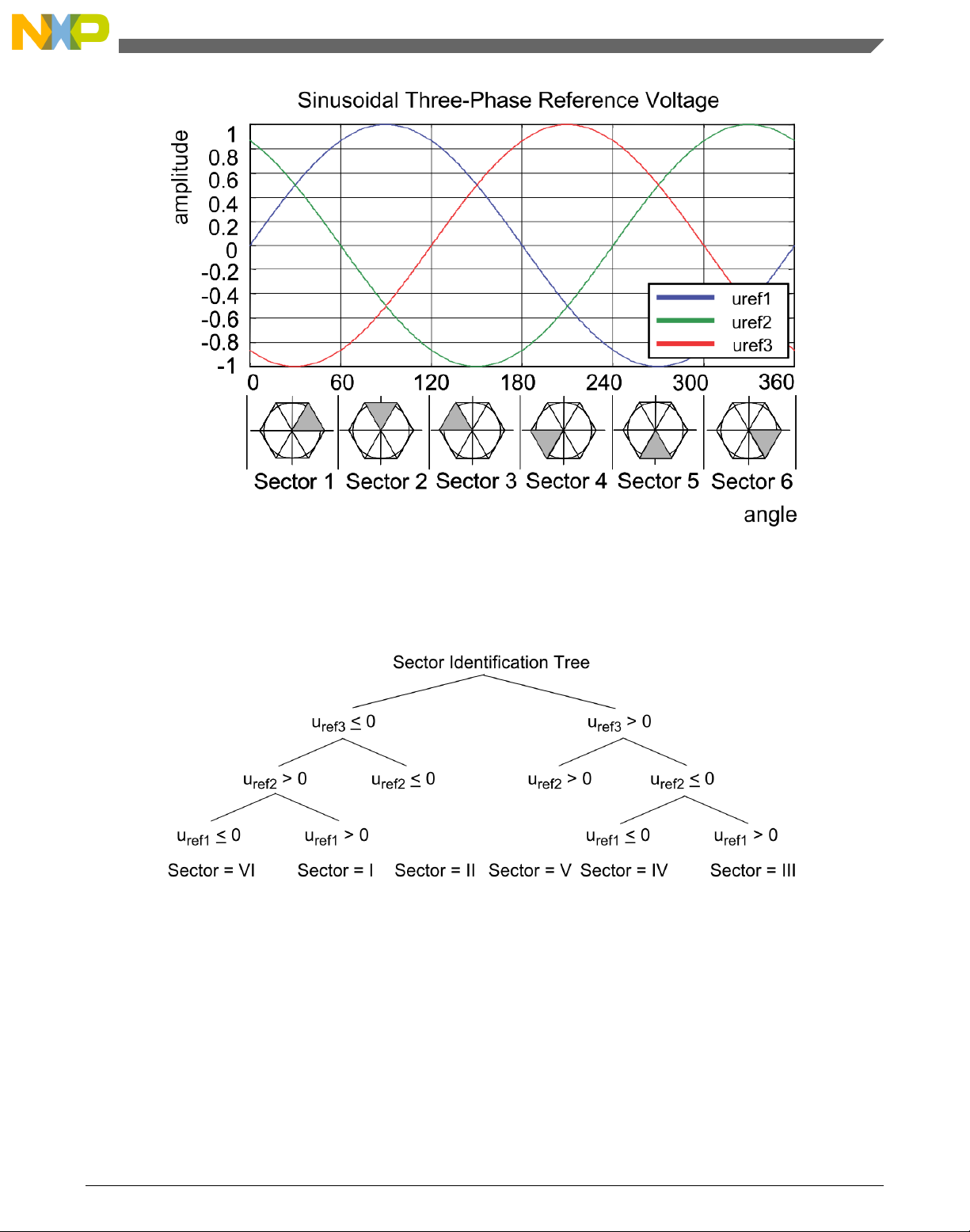
Figure 2-11. Direct-ua and quadrature-ub components of the stator reference voltage

Figure 2-11 depicts the direct-uα and quadrature-uβ components of the stator reference

voltage vector US, which were calculated using equations uα = cos ϑ and uβ = sin ϑ, respectively.

GMCLIB User's Guide, Rev. 2, 10/2015

46 Freescale Semiconductor, Inc.

Chapter 2 Algorithms in detail

Figure 2-12. Reference voltages U

ref1

, U

ref2

, and U

ref3

The sector identification tree shown in Figure 2-13 can be a numerical solution of the approach shown in GMCLIB_SvmStd_Img8.

Figure 2-13. Identification of the sector number

In the worst case, at least three simple comparisons are required to precisely identify the sector of the stator reference voltage vector. For example, if the stator reference voltage vector is located as shown in Figure 2-7, the stator-reference voltage vector is phaseadvanced by 30° from the direct α-axis, which results in the positive quantities of u and u

, and the negative quantity of u

ref2

; see Figure 2-12. If these quantities are used

ref3

ref1

as the inputs for the sector identification tree, the product of those comparisons will be sector I. The same approach identifies sector II, if the stator-reference voltage vector is

GMCLIB User's Guide, Rev. 2, 10/2015

Freescale Semiconductor, Inc. 47

GMCLIB_SvmStd

located as shown in Figure 2-9. The variables t1, t2, and t3, which represent the switching duty-cycle ratios of the respective three-phase system, are calculated according to the following equations:

Equation 42

where T is the switching period, and t_1 and t_2 are the duty-cycle ratios of the basic space vectors given for the respective sector; Table 2-10, Equation 31 on page 38, and

Equation 42 on page 48 are specific solely to the standard space vector modulation

technique; other space vector modulation techniques discussed later will require deriving different equations.

The next step is to assign the correct duty-cycle ratios - t1, t2, and t3, to the respective motor phases. This is a simple task, accomplished in a view of the position of the stator reference voltage vector; see Table 4.

Table 2-11. Assignment of the duty-cycle ratios to motor phases

Sectors U0, U

pwm_a t pwm_b t pwm_c t

U60, U

120

, U

t t t

180

, U

t t t

240

, U

t t t

300

, U

300

The principle of the space vector modulation technique consists of applying the basic voltage vectors U

XXX

and O

for certain time, in such a way that the main vector

XXX

generated by the pulse width modulation approach for the period T is equal to the original stator reference voltage vector US. This provides a great variability of arrangement of the basic vectors during the PWM period T. These vectors might be arranged either to lower the switching losses, or to achieve diverse results, such as center-aligned PWM, edgealigned PWM, or a minimal number of switching states. A brief discussion of the widely used center-aligned PWM follows.

Generating the center-aligned PWM pattern is accomplished by comparing the threshold levels pwm_a, pwm_b, and pwm_c with a free-running up-down counter. The timer counts to one, and then down to zero. It is supposed that when a threshold level is larger than the timer value, the respective PWM output is active. Otherwise, it is inactive; see

Figure 2-14.

GMCLIB User's Guide, Rev. 2, 10/2015

48 Freescale Semiconductor, Inc.

Chapter 2 Algorithms in detail

Figure 2-14. Standard space vector modulation technique — center-aligned PWM

Figure 2-15 shows the waveforms of the duty-cycle ratios, calculated using standard

space vector modulation. For the accurate calculation of the duty-cycle ratios, direct-α, and quadrature-β

components of the stator reference voltage vector, it must be considered that the duty cycle cannot be higher than one (100 %); in other words, the assumption must be

met.

GMCLIB User's Guide, Rev. 2, 10/2015

Freescale Semiconductor, Inc. 49

GMCLIB_SvmStd

Figure 2-15. Standard space vector modulation technique

2.8.1

Available versions

This function is available in the following versions:

• Fractional output - the output is the fractional portion of the result; the result is within the range <0 ; 1). The result may saturate.

GMCLIB User's Guide, Rev. 2, 10/2015

50 Freescale Semiconductor, Inc.

Chapter 2 Algorithms in detail

The available versions of the GMCLIB_SvmStd function are shown in the following table.

Table 2-12. Function versions

Function name Input type Output type Result type

GMCLIB_SvmStd_F16 GMCLIB_2COOR_ALBE_T_F16 * GMCLIB_3COOR_T_F16 * uint16_t

Standard space vector modulation with a 16-bit fractional stationary (α-β) input and a 16-bit fractional three-phase output. The result type is a 16-bit unsigned integer, which indicates the actual SVM sector. The input is within the range <-1 ; 1); the output duty cycle is within the range <0 ; 1). The output sector is an integer value within the range <0 ; 7>.

2.8.2 Declaration

The available GMCLIB_SvmStd functions have the following declarations:

uint16_t GMCLIB_SvmStd_F16(const GMCLIB_2COOR_ALBE_T_F16 *psIn, GMCLIB_3COOR_T_F16 *psOut)

2.8.3

Function use

The use of the GMCLIB_SvmStd function is shown in the following example:

#include "gmclib.h"

static uint16_t u16Sector; static GMCLIB_2COOR_ALBE_T_F16 sAlphaBeta; static GMCLIB_3COOR_T_F16 sAbc;

void Isr(void);

void main(void) { /* Alpha, Beta structure initialization */ sAlphaBeta.f16Alpha = FRAC16(0.0); sAlphaBeta.f16Beta = FRAC16(0.0); }

/* Periodical function or interrupt */ void Isr(void) { /* SVM calculation */ u16Sector = GMCLIB_SvmStd_F16(&sAlphaBeta, &sAbc); }

2.9

Freescale Semiconductor, Inc. 51

GMCLIB_SvmIct

GMCLIB User's Guide, Rev. 2, 10/2015

GMCLIB_SvmIct

The GMCLIB_SvmIct function calculates the appropriate duty-cycle ratios, which are needed for generation of the given stator-reference voltage vector using the general sinusoidal modulation technique.

The GMCLIB_SvmIct function calculates the appropriate duty-cycle ratios, needed for generation of the given stator reference voltage vector using the conventional Inverse Clark transformation. Finding the sector in which the reference stator voltage vector U resides is similar to GMCLIB_SvmStd. This is achieved by first converting the direct-α and the quadrature-β components of the reference stator voltage vector US into the balanced three-phase quantities u

ref1

, u

ref2

, and u

using the modified Inverse Clark

ref3

transformation:

Equation 43

The calculation of the sector number is based on comparing the three-phase reference voltages u

ref1

, u

ref2

, and u

with zero. This computation is described by the following

ref3

set of rules:

Equation 44

After passing these rules, the modified sector numbers are then derived using the following formula:

Equation 45

The sector numbers determined by this formula must be further transformed to correspond to those determined by the sector identification tree. The transformation which meets this requirement is shown in the following table:

Table 2-13. Transformation of the sectors

Sector* 1 2 3 4 5 6

Sector 2 6 1 4 3 5

GMCLIB User's Guide, Rev. 2, 10/2015

52 Freescale Semiconductor, Inc.

Chapter 2 Algorithms in detail

Use the Inverse Clark transformation for transforming values such as flux, voltage, and current from an orthogonal rotating coordination system (uα, uβ) to a three-phase rotating coordination system (ua, ub, and uc). The original equations of the Inverse Clark transformation are scaled here to provide the duty-cycle ratios in the range <0 ; 1). These scaled duty cycle ratios pwm_a, pwm_b, and pwm_c can be used directly by the registers of the PWM block.

Equation 46

The following figure shows the waveforms of the duty-cycle ratios calculated using the Inverse Clark transformation.

GMCLIB User's Guide, Rev. 2, 10/2015

Freescale Semiconductor, Inc. 53

GMCLIB_SvmIct

Figure 2-16. Inverse Clark transform modulation technique

For an accurate calculation of the duty-cycle ratios and the direct-α and quadrature-β components of the stator reference voltage vector, the duty cycle cannot be higher than

one (100 %); in other words, the assumption must be met.

2.9.1

Available versions

This function is available in the following versions:

• Fractional output - the output is the fractional portion of the result; the result is within the range <0 ; 1). The result may saturate.

GMCLIB User's Guide, Rev. 2, 10/2015

54 Freescale Semiconductor, Inc.

Chapter 2 Algorithms in detail

The available versions of the GMCLIB_SvmIct function are shown in the following table:

Table 2-14. Function versions

Function name Input type Output type Result type

GMCLIB_SvmIct_F16 GMCLIB_2COOR_ALBE_T_F16 * GMCLIB_3COOR_T_F16 * uint16_t

General sinusoidal space vector modulation with a 16-bit fractional stationary (α-β) input and a 16-bit fractional three-phase output. The result type is a 16-bit unsigned integer, which indicates the actual SVM sector. The input is within the range <-1 ; 1); the output duty cycle is within the range <0 ; 1). The output sector is an integer value within the range <0 ; 7>.

2.9.2 Declaration

The available GMCLIB_SvmIct functions have the following declarations:

uint16_t GMCLIB_SvmIct_F16(const GMCLIB_2COOR_ALBE_T_F16 *psIn, GMCLIB_3COOR_T_F16 *psOut)

2.9.3

Function use

The use of the GMCLIB_SvmIct function is shown in the following example:

#include "gmclib.h"

static uint16_t u16Sector; static GMCLIB_2COOR_ALBE_T_F16 sAlphaBeta; static GMCLIB_3COOR_T_F16 sAbc;

void Isr(void);

void main(void) { /* Alpha, Beta structure initialization */ sAlphaBeta.f16Alpha = FRAC16(0.0); sAlphaBeta.f16Beta = FRAC16(0.0); }

/* Periodical function or interrupt */ void Isr(void) { /* SVM calculation */ u16Sector = GMCLIB_SvmIct_F16(&sAlphaBeta, &sAbc); }

2.10

Freescale Semiconductor, Inc. 55

GMCLIB_SvmU0n

GMCLIB User's Guide, Rev. 2, 10/2015

GMCLIB_SvmU0n

The GMCLIB_SvmU0n function calculates the appropriate duty-cycle ratios, which are needed for generation of the given stator-reference voltage vector using the general sinusoidal modulation technique.

The GMCLIB_SvmU0n function for calculating of duty-cycle ratios is widely used in modern electric drives. This function calculates the appropriate duty-cycle ratios, which are needed for generating the given stator reference voltage vector using a special space vector modulation technique called space vector modulation with O one type of null vector O

is used (all bottom switches are turned on in the invertor).

000

nulls, where only

000

The derivation approach of the space vector modulation technique with O

nulls is in

000

many aspects identical to the approach presented in GMCLIB_SvmStd. However, a distinct difference lies in the definition of the variables t1, t2, and t3 that represent switching duty-cycle ratios of the respective phases:

Equation 47

where T is the switching period, and t_1 and t_2 are the duty-cycle ratios of the basic space vectors that are defined for the respective sector in Table 2-10.

The generally used center-aligned PWM is discussed briefly in the following sections. Generating the center-aligned PWM pattern is accomplished practically by comparing the threshold levels pwm_a, pwm_b, and pwm_c with the free-running up/down counter. The timer counts up to 1 (0x7FFF) and then down to 0 (0x0000). It is supposed that when a threshold level is larger than the timer value, the respective PWM output is active. Otherwise it is inactive (see Figure 2-17).

GMCLIB User's Guide, Rev. 2, 10/2015

56 Freescale Semiconductor, Inc.

Chapter 2 Algorithms in detail

Figure 2-17. Space vector modulation technique with O

nulls — center-aligned PWM

000

Figure Figure 2-17 shows calculated waveforms of the duty cycle ratios using space vector modulation with O

000

nulls.

For an accurate calculation of the duty-cycle ratios, direct-α, and quadrature-β components of the stator reference voltage vector, consider that the duty cycle cannot be

higher than one (100 %); in other words, the assumption must be met.

GMCLIB User's Guide, Rev. 2, 10/2015

Freescale Semiconductor, Inc. 57

GMCLIB_SvmU0n

2.10.1

Figure 2-18. Space vector modulation technique with O

Available versions

000

nulls

This function is available in the following versions:

• Fractional output - the output is the fractional portion of the result; the result is within the range <0 ; 1). The result may saturate.

GMCLIB User's Guide, Rev. 2, 10/2015

58 Freescale Semiconductor, Inc.

Chapter 2 Algorithms in detail

The available versions of the GMCLIB_SvmU0n function are shown in the following table:

Table 2-15. Function versions

Function name Input type Output type Result type

GMCLIB_SvmU0n_F16 GMCLIB_2COOR_ALBE_T_F16 * GMCLIB_3COOR_T_F16 * uint16_t

General sinusoidal space vector modulation with a 16-bit fractional stationary (α-β) input, and a 16-bit fractional three-phase output. The result type is a 16-bit unsigned integer, which indicates the actual SVM sector. The input is within the range <-1 ; 1); the output duty cycle is within the range <0 ; 1). The output sector is an integer value within the range <0 ; 7>.

2.10.2 Declaration

The available GMCLIB_SvmU0n functions have the following declarations:

uint16_t GMCLIB_SvmU0n_F16(const GMCLIB_2COOR_ALBE_T_F16 *psIn, GMCLIB_3COOR_T_F16 *psOut)

2.10.3

Function use

The use of the GMCLIB_SvmU0n function is shown in the following example:

#include "gmclib.h"

static uint16_t u16Sector; static GMCLIB_2COOR_ALBE_T_F16 sAlphaBeta; static GMCLIB_3COOR_T_F16 sAbc;

void Isr(void);

void main(void) { /* Alpha, Beta structure initialization */ sAlphaBeta.f16Alpha = FRAC16(0.0); sAlphaBeta.f16Beta = FRAC16(0.0); }

/* Periodical function or interrupt */ void Isr(void) { /* SVM calculation */ u16Sector = GMCLIB_SvmU0n_F16(&sAlphaBeta, &sAbc); }

2.11

Freescale Semiconductor, Inc. 59

GMCLIB_SvmU7n

GMCLIB User's Guide, Rev. 2, 10/2015

GMCLIB_SvmU7n

The GMCLIB_SvmU7n function calculates the appropriate duty-cycle ratios, which are needed for generation of the given stator-reference voltage vector, using the general sinusoidal modulation technique.

The GMCLIB_SvmU7n function for calculating the duty-cycle ratios is widely used in modern electric drives. This function calculates the appropriate duty-cycle ratios, which are needed for generating the given stator reference voltage vector using a special space vector modulation technique called space vector modulation with O one type of null vector O

is used (all top switches are turned on in the invertor).

111

nulls, where only

111

The derivation approach of the space vector modulation technique with O

nulls is

111

identical (in many aspects) to the approach presented in GMCLIB_SvmStd. However, a distinct difference lies in the definition of variables t1, t2, and t3 that represent switching duty-cycle ratios of the respective phases:

Equation 48

where T is the switching period, and t_1 and t_2 are the duty-cycle ratios of the basic space vectors defined for the respective sector in Table 2-10.

The generally-used center-aligned PWM is discussed briefly in the following sections. Generating the center-aligned PWM pattern is accomplished by comparing threshold levels pwm_a, pwm_b, and pwm_c with the free-running up/down counter. The timer counts up to 1 (0x7FFF) and then down to 0 (0x0000). It is supposed that when a threshold level is larger than the timer value, the respective PWM output is active. Otherwise, it is inactive (see Figure 2-19).

GMCLIB User's Guide, Rev. 2, 10/2015

60 Freescale Semiconductor, Inc.

Chapter 2 Algorithms in detail

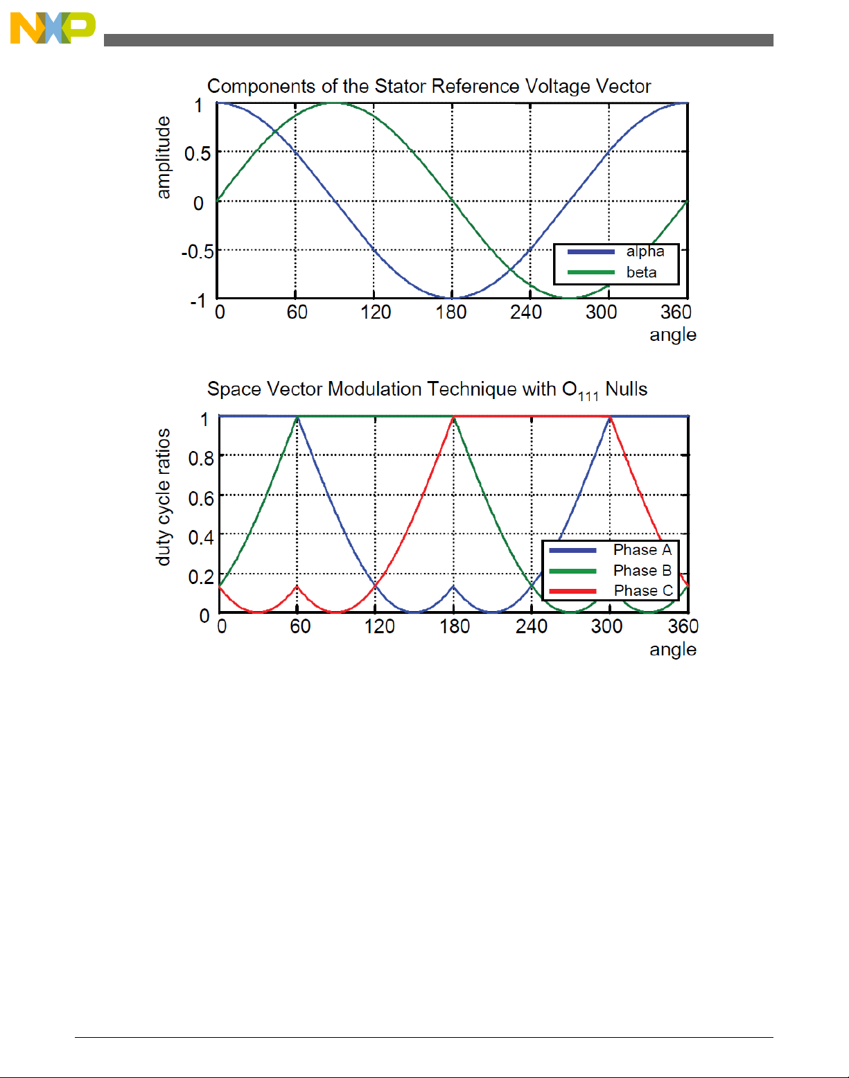
Figure 2-19. Space vector modulation technique with O

nulls — center-aligned PWM

111

Figure Figure 2-19 shows calculated waveforms of the duty-cycle ratios using Space Vector Modulation with O

111

nulls.

For an accurate calculation of the duty-cycle ratios, direct-α, and quadrature-β components of the stator reference voltage vector, it must be considered that the duty

cycle cannot be higher than one (100 %); in other words, the assumption

must be

met.

GMCLIB User's Guide, Rev. 2, 10/2015

Freescale Semiconductor, Inc. 61

GMCLIB_SvmU7n

2.11.1

Figure 2-20. Space vector modulation technique with O

Available versions

111

nulls

This function is available in the following versions:

• Fractional output - the output is the fractional portion of the result; the result is within the range <0 ; 1). The result may saturate.

GMCLIB User's Guide, Rev. 2, 10/2015

62 Freescale Semiconductor, Inc.

Chapter 2 Algorithms in detail

The available versions of the GMCLIB_SvmU7n function are shown in the following table:

Table 2-16. Function versions

Function name Input type Output type Result type

GMCLIB_SvmU7n_F16 GMCLIB_2COOR_ALBE_T_F16 * GMCLIB_3COOR_T_F16 * uint16_t

2.11.2 Declaration

The available GMCLIB_SvmU7n functions have the following declarations:

uint16_t GMCLIB_SvmU7n_F16(const GMCLIB_2COOR_ALBE_T_F16 *psIn, GMCLIB_3COOR_T_F16 *psOut)

2.11.3

Function use

The use of the GMCLIB_SvmU7n function is shown in the following example:

#include "gmclib.h"

static uint16_t u16Sector; static GMCLIB_2COOR_ALBE_T_F16 sAlphaBeta; static GMCLIB_3COOR_T_F16 sAbc;

void Isr(void);

void main(void) { /* Alpha, Beta structure initialization */ sAlphaBeta.f16Alpha = FRAC16(0.0); sAlphaBeta.f16Beta = FRAC16(0.0); }

/* Periodical function or interrupt */ void Isr(void) { /* SVM calculation */ u16Sector = GMCLIB_SvmU7n_F16(&sAlphaBeta, &sAbc); }

GMCLIB User's Guide, Rev. 2, 10/2015

Freescale Semiconductor, Inc. 63

GMCLIB_SvmU7n

GMCLIB User's Guide, Rev. 2, 10/2015

64 Freescale Semiconductor, Inc.

Appendix A Library types

A.1 bool_t

The

bool_t type is a logical 16-bit type. It is able to store the boolean variables with two

states: TRUE (1) or FALSE (0). Its definition is as follows:

typedef unsigned short bool_t;

The following figure shows the way in which the data is stored by this type:

Table A-1. Data storage

15 14 13 12 11 10 9 8 7 6 5 4 3 2 1 0

Value Unused

TRUE

FALSE

0 0 0 0 0 0 0 0 0 0 0 0 0 0 0 1

0 0 0 1

0 0 0 0 0 0 0 0 0 0 0 0 0 0 0 0

0 0 0 0

Logi

cal

To store a logical value as bool_t, use the FALSE or TRUE macros.

A.2

uint8_t

The uint8_t type is an unsigned 8-bit integer type. It is able to store the variables within the range <0 ; 255>. Its definition is as follows:

typedef unsigned char int8_t;

The following figure shows the way in which the data is stored by this type:

GMCLIB User's Guide, Rev. 2, 10/2015

Freescale Semiconductor, Inc. 65

uint16_t

Table A-2. Data storage

7 6 5 4 3 2 1 0

Value Integer

255

124

159

1 1 1 1 1 1 1 1

F F

0 0 0 0 1 0 1 1

0 B

0 1 1 1 1 1 0 0

7 C

1 0 0 1 1 1 1 1

9 F

A.3 uint16_t

The uint16_t type is an unsigned 16-bit integer type. It is able to store the variables within the range <0 ; 65535>. Its definition is as follows:

typedef unsigned short uint16_t;

The following figure shows the way in which the data is stored by this type:

Table A-3. Data storage

15 14 13 12 11 10 9 8 7 6 5 4 3 2 1 0

Value Integer

65535

15518

40768

1 1 1 1 1 1 1 1 1 1 1 1 1 1 1 1

F F F F

0 0 0 0 0 0 0 0 0 0 0 0 0 1 0 1

0 0 0 5

0 0 1 1 1 1 0 0 1 0 0 1 1 1 1 0

3 C 9 E

1 0 0 1 1 1 1 1 0 1 0 0 0 0 0 0

9 F 4 0

A.4 uint32_t

GMCLIB User's Guide, Rev. 2, 10/2015

66 Freescale Semiconductor, Inc.

Appendix A Library types

The uint32_t type is an unsigned 32-bit integer type. It is able to store the variables within the range <0 ; 4294967295>. Its definition is as follows:

typedef unsigned long uint32_t;

The following figure shows the way in which the data is stored by this type:

Table A-4. Data storage

31 24 23 16 15 8 7 0

Value Integer 4294967295 F F F F F F F F 2147483648 8 0 0 0 0 0 0 0

55977296 0 3 5 6 2 5 5 0

3451051828 C D B 2 D F 3 4

A.5 int8_t

The int8_t type is a signed 8-bit integer type. It is able to store the variables within the range <-128 ; 127>. Its definition is as follows:

typedef char int8_t;

The following figure shows the way in which the data is stored by this type:

Table A-5. Data storage

7 6 5 4 3 2 1 0

Value Sign Integer

127

-128

-97

0 1 1 1 1 1 1 1

7 F

1 0 0 0 0 0 0 0

8 0

0 0 1 1 1 1 0 0

3 C

1 0 0 1 1 1 1 1

9 F

GMCLIB User's Guide, Rev. 2, 10/2015

Freescale Semiconductor, Inc. 67

int16_t

A.6 int16_t

The int16_t type is a signed 16-bit integer type. It is able to store the variables within the range <-32768 ; 32767>. Its definition is as follows:

typedef short int16_t;

The following figure shows the way in which the data is stored by this type:

Table A-6. Data storage

15 14 13 12 11 10 9 8 7 6 5 4 3 2 1 0

Value Sign Integer

32767

-32768

15518

-24768

0 1 1 1 1 1 1 1 1 1 1 1 1 1 1 1

7 F F F

1 0 0 0 0 0 0 0 0 0 0 0 0 0 0 0

8 0 0 0

0 0 1 1 1 1 0 0 1 0 0 1 1 1 1 0

3 C 9 E

1 0 0 1 1 1 1 1 0 1 0 0 0 0 0 0

9 F 4 0

A.7 int32_t

The int32_t type is a signed 32-bit integer type. It is able to store the variables within the range <-2147483648 ; 2147483647>. Its definition is as follows:

typedef long int32_t;

The following figure shows the way in which the data is stored by this type:

Table A-7. Data storage

31 24 23 16 15 8 7 0

Value S Integer 2147483647 7 F F F F F F F

-2147483648 8 0 0 0 0 0 0 0 55977296 0 3 5 6 2 5 5 0

-843915468 C D B 2 D F 3 4

GMCLIB User's Guide, Rev. 2, 10/2015

68 Freescale Semiconductor, Inc.

Appendix A Library types

A.8 frac8_t

The frac8_t type is a signed 8-bit fractional type. It is able to store the variables within the range <-1 ; 1). Its definition is as follows:

typedef char frac8_t;

The following figure shows the way in which the data is stored by this type:

Table A-8. Data storage

7 6 5 4 3 2 1 0

Value Sign Fractional

0.99219

-1.0

0.46875

-0.75781

0 1 1 1 1 1 1 1

7 F

1 0 0 0 0 0 0 0

8 0

0 0 1 1 1 1 0 0

3 C

1 0 0 1 1 1 1 1

9 F

To store a real number as frac8_t, use the FRAC8 macro.

A.9

frac16_t

The frac16_t type is a signed 16-bit fractional type. It is able to store the variables within the range <-1 ; 1). Its definition is as follows:

typedef short frac16_t;

The following figure shows the way in which the data is stored by this type:

Table A-9. Data storage

15 14 13 12 11 10 9 8 7 6 5 4 3 2 1 0

Value Sign Fractional

0.99997

-1.0 1 0 0 0 0 0 0 0 0 0 0 0 0 0 0 0

0 1 1 1 1 1 1 1 1 1 1 1 1 1 1 1

7 F F F

Table continues on the next page...

GMCLIB User's Guide, Rev. 2, 10/2015

Freescale Semiconductor, Inc. 69

frac32_t

Table A-9. Data storage (continued)

8 0 0 0

0.47357

-0.75586

0 0 1 1 1 1 0 0 1 0 0 1 1 1 1 0

3 C 9 E

1 0 0 1 1 1 1 1 0 1 0 0 0 0 0 0

9 F 4 0

To store a real number as frac16_t, use the FRAC16 macro.

A.10

The

frac32_t

frac32_t type is a signed 32-bit fractional type. It is able to store the variables within

the range <-1 ; 1). Its definition is as follows:

typedef long frac32_t;

The following figure shows the way in which the data is stored by this type:

Table A-10. Data storage

31 24 23 16 15 8 7 0

Value S Fractional

0.9999999995 7 F F F F F F F

-1.0 8 0 0 0 0 0 0 0

0.02606645970 0 3 5 6 2 5 5 0

-0.3929787632 C D B 2 D F 3 4

To store a real number as frac32_t, use the FRAC32 macro.

A.11

acc16_t

The acc16_t type is a signed 16-bit fractional type. It is able to store the variables within the range <-256 ; 256). Its definition is as follows:

typedef short acc16_t;

The following figure shows the way in which the data is stored by this type:

GMCLIB User's Guide, Rev. 2, 10/2015

70 Freescale Semiconductor, Inc.

Table A-11. Data storage

15 14 13 12 11 10 9 8 7 6 5 4 3 2 1 0

Value Sign Integer Fractional

255.9921875

-256.0

1.0

-1.0

13.7890625

-89.71875

0 1 1 1 1 1 1 1 1 1 1 1 1 1 1 1

7 F F F

1 0 0 0 0 0 0 0 0 0 0 0 0 0 0 0

8 0 0 0

0 0 0 0 0 0 0 0 1 0 0 0 0 0 0 0

0 0 8 0

1 1 1 1 1 1 1 1 1 0 0 0 0 0 0 0

F F 8 0

0 0 0 0 0 1 1 0 1 1 1 0 0 1 0 1

0 6 E 5

1 1 0 1 0 0 1 1 0 0 1 0 0 1 0 0

D 3 2 4

Appendix A Library types

To store a real number as acc16_t, use the ACC16 macro.

A.12

acc32_t

The acc32_t type is a signed 32-bit accumulator type. It is able to store the variables within the range <-65536 ; 65536). Its definition is as follows:

typedef long acc32_t;

The following figure shows the way in which the data is stored by this type:

Table A-12. Data storage

31 24 23 16 15 8 7 0

Value S Integer Fractional

65535.999969 7 F F F F F F F

-65536.0 8 0 0 0 0 0 0 0

1.0 0 0 0 0 8 0 0 0

-1.0 F F F F 8 0 0 0

23.789734 0 0 0 B E 5 1 6

-1171.306793 F D B 6 5 8 B C

To store a real number as acc32_t, use the ACC32 macro.

GMCLIB User's Guide, Rev. 2, 10/2015

Freescale Semiconductor, Inc. 71

GMCLIB_3COOR_T_F16

A.13 GMCLIB_3COOR_T_F16

The GMCLIB_3COOR_T_F16 structure type corresponds to the three-phase stationary coordinate system, based on the A, B, and C components. Each member is of the frac16_t data type. The structure definition is as follows:

typedef struct { frac16_t f16A; frac16_t f16B; frac16_t f16C; } GMCLIB_3COOR_T_F16;

The structure description is as follows:

Table A-13. GMCLIB_3COOR_T_F16 members description

Type Name Description

frac16_t f16A A component; 16-bit fractional type frac16_t f16B B component; 16-bit fractional type frac16_t f16C C component; 16-bit fractional type

A.14 GMCLIB_2COOR_ALBE_T_F16

The GMCLIB_2COOR_ALBE_T_F16 structure type corresponds to the two-phase stationary coordinate system, based on the Alpha and Beta orthogonal components. Each member is of the frac16_t data type. The structure definition is as follows:

typedef struct { frac16_t f16Alpha; frac16_t f16Beta; } GMCLIB_2COOR_ALBE_T_F16;

The structure description is as follows:

Table A-14. GMCLIB_2COOR_ALBE_T_F16 members description

Type Name Description

frac16_t f16Apha α-component; 16-bit fractional type frac16_t f16Beta β-component; 16-bit fractional type

GMCLIB User's Guide, Rev. 2, 10/2015

72 Freescale Semiconductor, Inc.

Appendix A Library types

A.15 GMCLIB_2COOR_DQ_T_F16

The GMCLIB_2COOR_DQ_T_F16 structure type corresponds to the two-phase rotating coordinate system, based on the D and Q orthogonal components. Each member is of the

frac16_t data type. The structure definition is as follows:

typedef struct { frac16_t f16D; frac16_t f16Q; } GMCLIB_2COOR_DQ_T_F16;

The structure description is as follows:

Table A-15. GMCLIB_2COOR_DQ_T_F16 members description

Type Name Description

frac16_t f16D D-component; 16-bit fractional type frac16_t f16Q Q-component; 16-bit fractional type

A.16 GMCLIB_2COOR_DQ_T_F32

The GMCLIB_2COOR_DQ_T_F32 structure type corresponds to the two-phase rotating coordinate system, based on the D and Q orthogonal components. Each member is of the

frac32_t data type. The structure definition is as follows:

typedef struct { frac32_t f32D; frac32_t f32Q; } GMCLIB_2COOR_DQ_T_F32;

The structure description is as follows:

Table A-16. GMCLIB_2COOR_DQ_T_F32 members description

Type Name Description

frac32_t f32D D-component; 32-bit fractional type frac32_t f32Q Q-component; 32-bit fractional type

A.17 GMCLIB_2COOR_SINCOS_T_F16

GMCLIB User's Guide, Rev. 2, 10/2015

Freescale Semiconductor, Inc. 73

FALSE

The GMCLIB_2COOR_SINCOS_T_F16 structure type corresponds to the two-phase coordinate system, based on the Sin and Cos components of a certain angle. Each member is of the frac16_t data type. The structure definition is as follows:

typedef struct { frac16_t f16Sin; frac16_t f16Cos; } GMCLIB_2COOR_SINCOS_T_F16;

The structure description is as follows:

Table A-17. GMCLIB_2COOR_SINCOS_T_F16 members description

Type Name Description

frac16_t f16Sin Sin component; 16-bit fractional type frac16_t f16Cos Cos component; 16-bit fractional type

A.18 FALSE

The FALSE macro serves to write a correct value standing for the logical FALSE value of the bool_t type. Its definition is as follows:

#define FALSE ((bool_t)0)

#include "mlib.h"

static bool_t bVal;

void main(void) { bVal = FALSE; /* bVal = FALSE */ }

A.19

The TRUE macro serves to write a correct value standing for the logical TRUE value of the bool_t type. Its definition is as follows:

TRUE

#define TRUE ((bool_t)1)

#include "mlib.h"

static bool_t bVal;

GMCLIB User's Guide, Rev. 2, 10/2015

74 Freescale Semiconductor, Inc.

Appendix A Library types

void main(void) { bVal = TRUE; /* bVal = TRUE */ }

A.20 FRAC8

The FRAC8 macro serves to convert a real number to the frac8_t type. Its definition is as follows:

#define FRAC8(x) ((frac8_t)((x) < 0.9921875 ? ((x) >= -1 ? (x)*0x80 : 0x80) : 0x7F))

The input is multiplied by 128 (=27). The output is limited to the range <0x80 ; 0x7F>, which corresponds to <-1.0 ; 1.0-2-7>.

#include "mlib.h"

static frac8_t f8Val;

void main(void) { f8Val = FRAC8(0.187); /* f8Val = 0.187 */ }

A.21

FRAC16

The FRAC16 macro serves to convert a real number to the frac16_t type. Its definition is as follows:

#define FRAC16(x) ((frac16_t)((x) < 0.999969482421875 ? ((x) >= -1 ? (x)*0x8000 : 0x8000) : 0x7FFF))

The input is multiplied by 32768 (=215). The output is limited to the range <0x8000 ; 0x7FFF>, which corresponds to <-1.0 ; 1.0-2

#include "mlib.h"

static frac16_t f16Val;

void main(void) { f16Val = FRAC16(0.736); /* f16Val = 0.736 */ }

-15

GMCLIB User's Guide, Rev. 2, 10/2015

Freescale Semiconductor, Inc. 75

FRAC32

A.22 FRAC32

The FRAC32 macro serves to convert a real number to the frac32_t type. Its definition is as follows:

#define FRAC32(x) ((frac32_t)((x) < 1 ? ((x) >= -1 ? (x)*0x80000000 : 0x80000000) : 0x7FFFFFFF))

The input is multiplied by 2147483648 (=231). The output is limited to the range <0x80000000 ; 0x7FFFFFFF>, which corresponds to <-1.0 ; 1.0-2

#include "mlib.h"

static frac32_t f32Val;

void main(void) { f32Val = FRAC32(-0.1735667); /* f32Val = -0.1735667 */ }

-31

A.23

ACC16

The ACC16 macro serves to convert a real number to the acc16_t type. Its definition is as follows:

#define ACC16(x) ((acc16_t)((x) < 255.9921875 ? ((x) >= -256 ? (x)*0x80 : 0x8000) : 0x7FFF))

The input is multiplied by 128 (=27). The output is limited to the range <0x8000 ; 0x7FFF> that corresponds to <-256.0 ; 255.9921875>.

#include "mlib.h"

static acc16_t a16Val;

void main(void) { a16Val = ACC16(19.45627); /* a16Val = 19.45627 */ }

A.24

ACC32

The ACC32 macro serves to convert a real number to the acc32_t type. Its definition is as follows:

GMCLIB User's Guide, Rev. 2, 10/2015

76 Freescale Semiconductor, Inc.

#define ACC32(x) ((acc32_t)((x) < 65535.999969482421875 ? ((x) >= -65536 ? (x)*0x8000 : 0x80000000) : 0x7FFFFFFF))

The input is multiplied by 32768 (=215). The output is limited to the range <0x80000000 ; 0x7FFFFFFF>, which corresponds to <-65536.0 ; 65536.0-2

#include "mlib.h"

static acc32_t a32Val;

void main(void) { a32Val = ACC32(-13.654437); /* a32Val = -13.654437 */ }

-15

GMCLIB User's Guide, Rev. 2, 10/2015

Freescale Semiconductor, Inc. 77

GMCLIB User's Guide, Rev. 2, 10/2015

78 Freescale Semiconductor, Inc.

How to Reach Us:

Home Page:

freescale.com

Web Support:

freescale.com/support

Information in this document is provided solely to enable system and software implementers to use Freescale products. There are no express or implied copyright licenses granted hereunder to design or fabricate any integrated circuits based on the information in this document. Freescale reserves the right to make changes without further notice to any products herein.

Freescale makes no warranty, representation, or guarantee regarding the suitability of its products for any particular purpose, nor does Freescale assume any liability arising out of the application or use of any product or circuit, and specifically disclaims any and all liability, including without limitation consequential or incidental damages. “Typical” parameters that may be provided in Freescale data sheets and/or specifications can and do vary in different applications, and actual performance may vary over time. All operating parameters, including “typicals,” must be validated for each customer application by customer's technical experts. Freescale does not convey any license under its patent rights nor the rights of others. Freescale sells products pursuant to standard terms and conditions of sale, which can be found at the following address: www.freescale.com/salestermsandconditions.

Freescale and the Freescale logo are trademarks of Freescale Semiconductor, Inc. All other product or service names are the property of their respective owners.

Document Number DSP56800EGMCLIBUG

Revision 2, 10/2015

NXP Semiconductors DSP56800E User Manual

Specifications and Main Features

Frequently Asked Questions

User Manual

1.1 Introduction

1.1.1 Overview

Data types

1.1.3 API definition

1.1.4 Supported compilers

1.1.5 Special issues

Library integration into project (CodeWarrior™ Development Studio)

New project

Library path variable

Library folder addition

Library path setup

GMCLIB_Clark function calculates the Clarke transformation, which is used to

Available versions

GMCLIB_ClarkInv

2.1.3 Function use

2.2.1 Available versions

2.2.2 Declaration

Function use

GMCLIB_Park

Available versions

2.3.2 Declaration

2.3.3 Function use

GMCLIB_ParkInv

2.4.2 Declaration

Function use

2.5 GMCLIB_DecouplingPMSM

Available versions

2.5.2 GMCLIB_DECOUPLINGPMSM_T_A32 type description

2.5.3 Declaration

Function use

GMCLIB_ElimDcBusRipFOC

Available versions

2.6.2 Declaration

Function use

GMCLIB_ElimDcBusRip

Available versions

2.7.2 Declaration

Function use

GMCLIB_SvmStd

Available versions

2.8.2 Declaration

Function use

GMCLIB_SvmIct

Available versions

2.9.2 Declaration

Function use

GMCLIB_SvmU0n

Available versions

2.10.2 Declaration

Function use

GMCLIB_SvmU7n

Available versions

2.11.2 Declaration

Function use

bool_t type is a logical 16-bit type. It is able to store the boolean variables with two

uint8_t

uint16_t

A.4 uint32_t

A.5 int8_t

int16_t

A.7 int32_t

A.8 frac8_t

frac16_t

frac32_t

acc16_t

acc32_t

GMCLIB_3COOR_T_F16

A.14 GMCLIB_2COOR_ALBE_T_F16

A.15 GMCLIB_2COOR_DQ_T_F16

A.16 GMCLIB_2COOR_DQ_T_F32

A.17 GMCLIB_2COOR_SINCOS_T_F16

FALSE

TRUE

A.20 FRAC8

FRAC16

FRAC32