NXP GMCLIB User Manual

Download

GMCLIB User's Guide

ARM® Cortex® M33F

Document Number: CM33FGMCLIBUG

Rev. 4, 12/2020

GMCLIB User's Guide, Rev. 4, 12/2020

2 NXP Semiconductors

Contents

Section number Title Page

Chapter 1

Library

1.1 Introduction.................................................................................................................................................................... 5

1.2 Library integration into project (MCUXpresso IDE) ....................................................................................................8

1.3 Library integration into project (Keil µVision) ............................................................................................................. 17

1.4 Library integration into project (IAR Embedded Workbench) ..................................................................................... 25

Chapter 2

Algorithms in detail

2.1 GMCLIB_Clark..............................................................................................................................................................33

2.2 GMCLIB_ClarkInv........................................................................................................................................................ 35

2.3 GMCLIB_Park............................................................................................................................................................... 37

2.4 GMCLIB_ParkInv..........................................................................................................................................................39

2.5 GMCLIB_DecouplingPMSM........................................................................................................................................ 41

2.6 GMCLIB_ElimDcBusRipFOC...................................................................................................................................... 47

2.7 GMCLIB_ElimDcBusRip.............................................................................................................................................. 52

2.8 GMCLIB_SvmStd..........................................................................................................................................................57

2.9 GMCLIB_SvmIct...........................................................................................................................................................72

2.10 GMCLIB_SvmU0n........................................................................................................................................................ 76

2.11 GMCLIB_SvmU7n........................................................................................................................................................ 80

2.12 GMCLIB_SvmDpwm.................................................................................................................................................... 84

2.13 GMCLIB_SvmExDpwm................................................................................................................................................87

GMCLIB User's Guide, Rev. 4, 12/2020

NXP Semiconductors 3

GMCLIB User's Guide, Rev. 4, 12/2020

4 NXP Semiconductors

Chapter 1 Library

1.1 Introduction

1.1.1 Overview

This user's guide describes the General Motor Control Library (GMCLIB) for the family of ARM Cortex M33F core-based microcontrollers. This library contains optimized functions.

1.1.2

GMCLIB supports several data types: (un)signed integer, fractional, and accumulator, and floating point. The integer data types are useful for general-purpose computation; they are familiar to the MPU and MCU programmers. The fractional data types enable powerful numeric and digital-signal-processing algorithms to be implemented. The accumulator data type is a combination of both; that means it has the integer and fractional portions.The floating-point data types are capable of storing real numbers in wide dynamic ranges. The type is represented by binary digits and an exponent. The exponent allows scaling the numbers from extremely small to extremely big numbers. Because the exponent takes part of the type, the overall resolution of the number is reduced when compared to the fixed-point type of the same size.

The following list shows the integer types defined in the libraries:

• Unsigned 16-bit integer —<0 ; 65535> with the minimum resolution of 1

• Signed 16-bit integer —<-32768 ; 32767> with the minimum resolution of 1

• Unsigned 32-bit integer —<0 ; 4294967295> with the minimum resolution of 1

• Signed 32-bit integer —<-2147483648 ; 2147483647> with the minimum resolution

Data types

of 1

GMCLIB User's Guide, Rev. 4, 12/2020

NXP Semiconductors 5

Introduction

The following list shows the fractional types defined in the libraries:

• Fixed-point 16-bit fractional —<-1 ; 1 - 2

• Fixed-point 32-bit fractional —<-1 ; 1 - 2

-15

> with the minimum resolution of 2

-31

> with the minimum resolution of 2

-15

-31

The following list shows the accumulator types defined in the libraries:

• Fixed-point 16-bit accumulator —<-256.0 ; 256.0 - 2-7> with the minimum resolution of 2

• Fixed-point 32-bit accumulator —<-65536.0 ; 65536.0 - 2 resolution of 2

-7

-15

> with the minimum

The following list shows the floating-point types defined in the libraries:

• Floating point 32-bit single precision —<-3.40282 · 1038 ; 3.40282 · 1038> with the minimum resolution of 2

1.1.3

API definition

-23

GMCLIB uses the types mentioned in the previous section. To enable simple usage of the algorithms, their names use set prefixes and postfixes to distinguish the functions' versions. See the following example:

f32Result = MLIB_Mac_F32lss(f32Accum, f16Mult1, f16Mult2);

where the function is compiled from four parts:

• MLIB—this is the library prefix

• Mac—the function name—Multiply-Accumulate

• F32—the function output type

• lss—the types of the function inputs; if all the inputs have the same type as the output, the inputs are not marked

The input and output types are described in the following table:

Table 1-1. Input/output types

Type Output Input

frac16_t F16 s frac32_t F32 l acc32_t A32 a

float_t FLT f

GMCLIB User's Guide, Rev. 4, 12/2020

6 NXP Semiconductors

Chapter 1 Library

1.1.4 Supported compilers

GMCLIB for the ARM Cortex M33F core is written in C language or assembly language with C-callable interface depending on the specific function. The library is built and tested using the following compilers:

• MCUXpresso IDE

• IAR Embedded Workbench

• Keil µVision

For the MCUXpresso IDE, the library is delivered in the gmclib.a file. For the Kinetis Design Studio, the library is delivered in the gmclib.a file. For the IAR Embedded Workbench, the library is delivered in the gmclib.a file. For the Keil µVision, the library is delivered in the gmclib.lib file. The interfaces to the algorithms included in this library are combined into a single public

interface include file, gmclib.h. This is done to lower the number of files required to be included in your application.

1.1.5

Library configuration

GMCLIB for the ARM Cortex M33F core is written in C language or assembly language with C-callable interface depending on the specific function. Some functions from this library are inline type, which are compiled together with project using this library. The optimization level for inline function is usually defined by the specific compiler setting. It can cause an issue especially when high optimization level is set. Therefore the optimization level for all inline assembly written functions is defined by compiler pragmas using macros. The configuration header file RTCESL_cfg.h is located in: specific library folder\MLIB\Include. The optimization level can be changed by modifying the macro value for specific compiler. In case of any change the library functionality is not guaranteed.

Similarly as optimization level the PowerQuad DSP Coprocessor and Accelerator support can be disable or enable if it has not been done by defined symbol RTCESL_PQ_ON or RTCESL_PQ_OFF in project setting described in the PowerQuad DSP Coprocessor and Accelerator support cheaper for specific compiler.

GMCLIB User's Guide, Rev. 4, 12/2020

NXP Semiconductors 7

Library integration into project (MCUXpresso IDE)

1.1.6 Special issues

1. The equations describing the algorithms are symbolic. If there is positive 1, the number is the closest number to 1 that the resolution of the used fractional type allows. If there are maximum or minimum values mentioned, check the range allowed by the type of the particular function version.

2. The library functions that round the result (the API contains Rnd) round to nearest (half up).

1.2 Library integration into project (MCUXpresso IDE)

This section provides a step-by-step guide on how to quickly and easily include GMCLIB into any MCUXpresso SDK example or demo application projects using MCUXpresso IDE. This example uses the default installation path (C:\NXP\RTCESL \CM33F_RTCESL_4.6_MCUX). If you have a different installation path, use that path instead.

1.2.1

PowerQuad DSP Coprocessor and Accelerator support

Some LPC platforms (LPC55S6x) contain a hardware accelerator dedicated to common calculations in DSP applications. This section shows how to turn the PowerQuad (PQ) support for a function on and off.

1. In the MCUXpresso SDK project name node or in the left-hand part, click Properties or select Project > Properties from the menu. A project properties dialog appears.

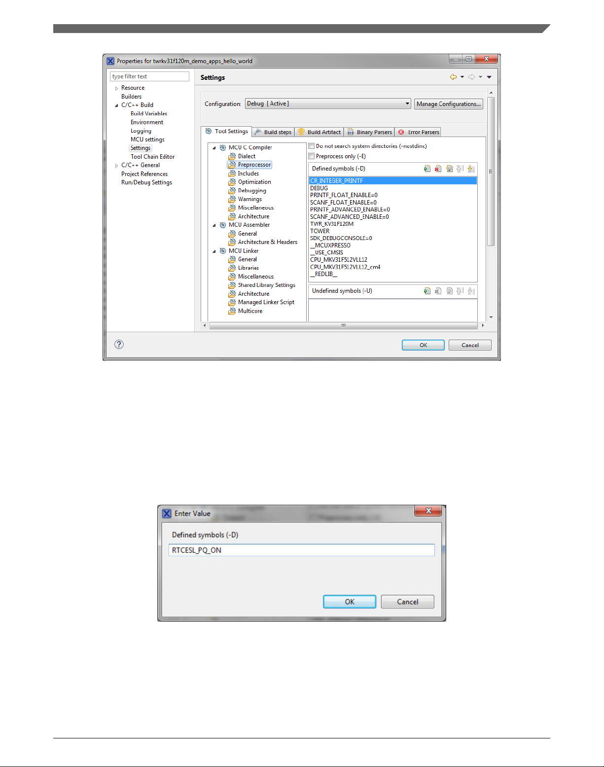
2. Expand the C/C++ Build node and select Settings. See .

3. On the right-hand side, under the MCU C Compiler node, click the Preprocessor node. See .

GMCLIB User's Guide, Rev. 4, 12/2020

8 NXP Semiconductors

Chapter 1 Library

Figure 1-1. Defined symbols

4. In the right-hand part of the dialog, click the Add... icon located next to the Defined symbols (-D) title.

5. In the dialog that appears (see ), type the following:

• RTCESL_PQ_ON—to turn the PowerQuad support on

• RTCESL_PQ_OFF—to turn the PowerQuad support off If neither of these two defines is defined, the hardware division and square root support is turned off by default.

Figure 1-2. Symbol definition

6. Click OK in the dialog.

7. Click OK in the main dialog.

8. Ensure the PowerQuad moduel to be clocked by calling function RTCESL_PQ_Init(); prior to the first function using PQ module calling.

GMCLIB User's Guide, Rev. 4, 12/2020

NXP Semiconductors 9

Library integration into project (MCUXpresso IDE)

See the device reference manual to verify whether the device contains the PowerQuad DSP Coprocessor and Accelerator support.

1.2.2 Library path variable

To make the library integration easier, create a variable that holds the information about the library path.

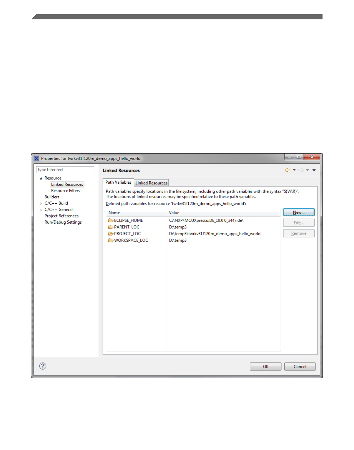
1. Right-click the MCUXpresso SDK project name node in the left-hand part and click Properties, or select Project > Properties from the menu. A project properties dialog appears.

2. Expand the Resource node and click Linked Resources. See Figure 1-3.

Figure 1-3. Project properties

3. Click the New… button in the right-hand side.

GMCLIB User's Guide, Rev. 4, 12/2020

10 NXP Semiconductors

Chapter 1 Library

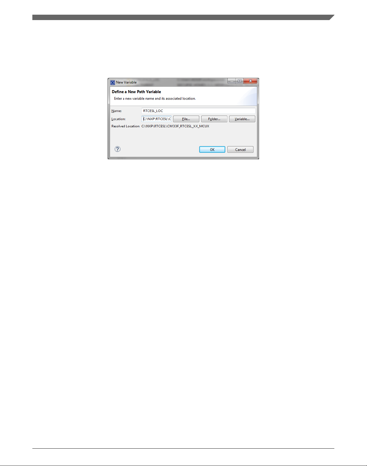
4. In the dialog that appears (see Figure 1-4), type this variable name into the Name box: RTCESL_LOC.

5. Select the library parent folder by clicking Folder…, or just type the following path into the Location box: C:\NXP\RTCESL\CM33F_RTCESL_4.6_MCUX. Click OK.

Figure 1-4. New variable

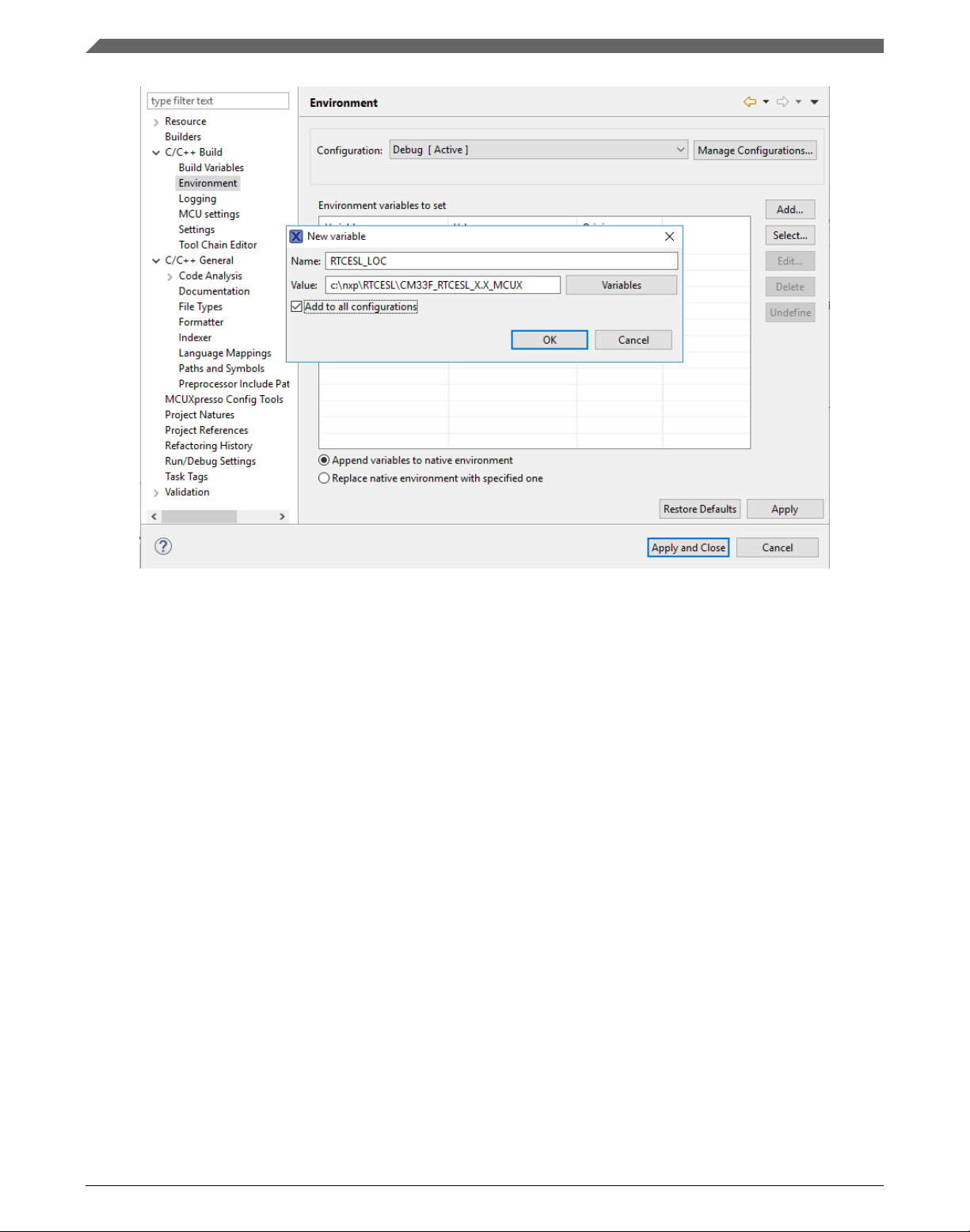
6. Create such variable for the environment. Expand the C/C++ Build node and click Environment.

7. Click the Add… button in the right-hand side.

8. In the dialog that appears (see Figure 1-5), type this variable name into the Name box: RTCESL_LOC.

9. Type the library parent folder path into the Value box: C:\NXP\RTCESL \CM33F_RTCESL_4.6_MCUX.

10. Tick the Add to all configurations box to use this variable in all configurations. See

Figure 1-5.

11. Click OK.

12. In the previous dialog, click OK.

GMCLIB User's Guide, Rev. 4, 12/2020

NXP Semiconductors 11

Library integration into project (MCUXpresso IDE)

Figure 1-5. Environment variable

1.2.3

Library folder addition

To use the library, add it into the Project tree dialog.

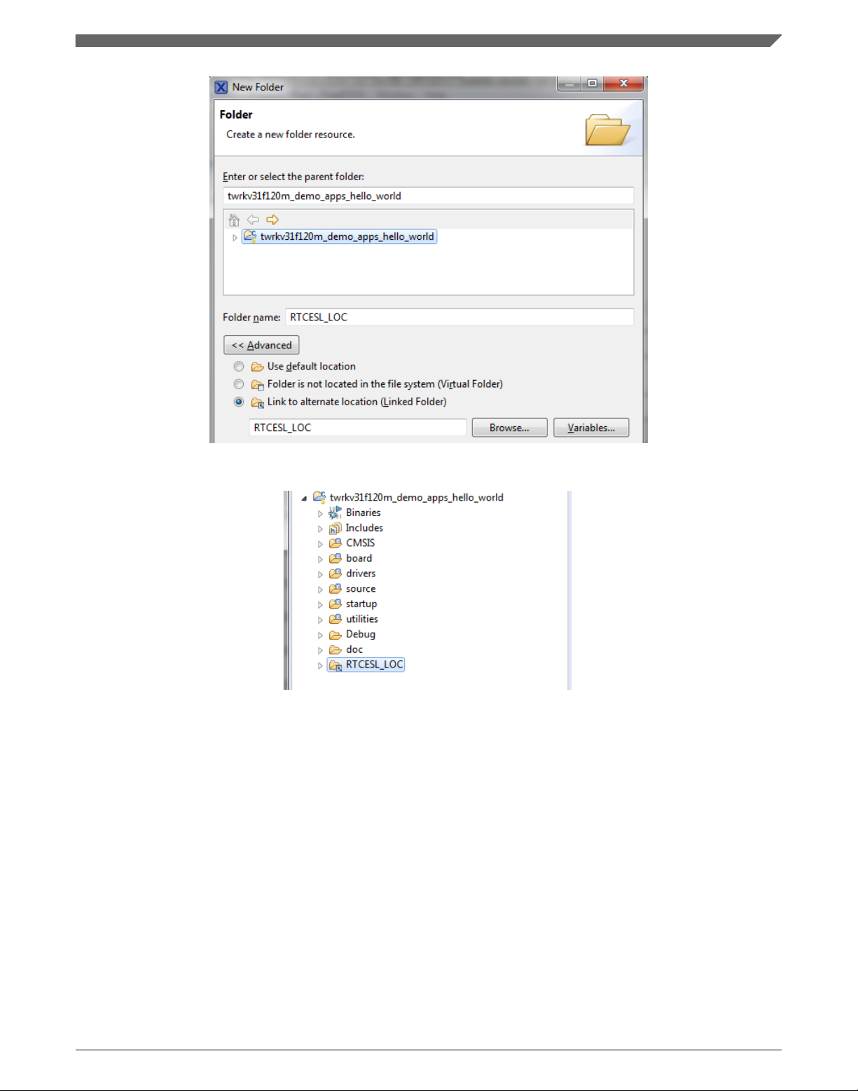
1. Right-click the MCUXpresso SDK project name node in the left-hand part and click New > Folder, or select File > New > Folder from the menu. A dialog appears.

2. Click Advanced to show the advanced options.

3. To link the library source, select the Link to alternate location (Linked Folder) option.

4. Click Variables..., select the RTCESL_LOC variable in the dialog, click OK, and/or type the variable name into the box. See Figure 1-6.

5. Click Finish, and the library folder is linked in the project. See Figure 1-7.

GMCLIB User's Guide, Rev. 4, 12/2020

12 NXP Semiconductors

Chapter 1 Library

Figure 1-6. Folder link

Figure 1-7. Projects libraries paths

1.2.4

Library path setup

GMCLIB requires MLIB and GFLIB to be included too. These steps show how to include all dependent modules:

1. Right-click the MCUXpresso SDK project name node in the left-hand part and click Properties, or select Project > Properties from the menu. The project properties dialog appears.

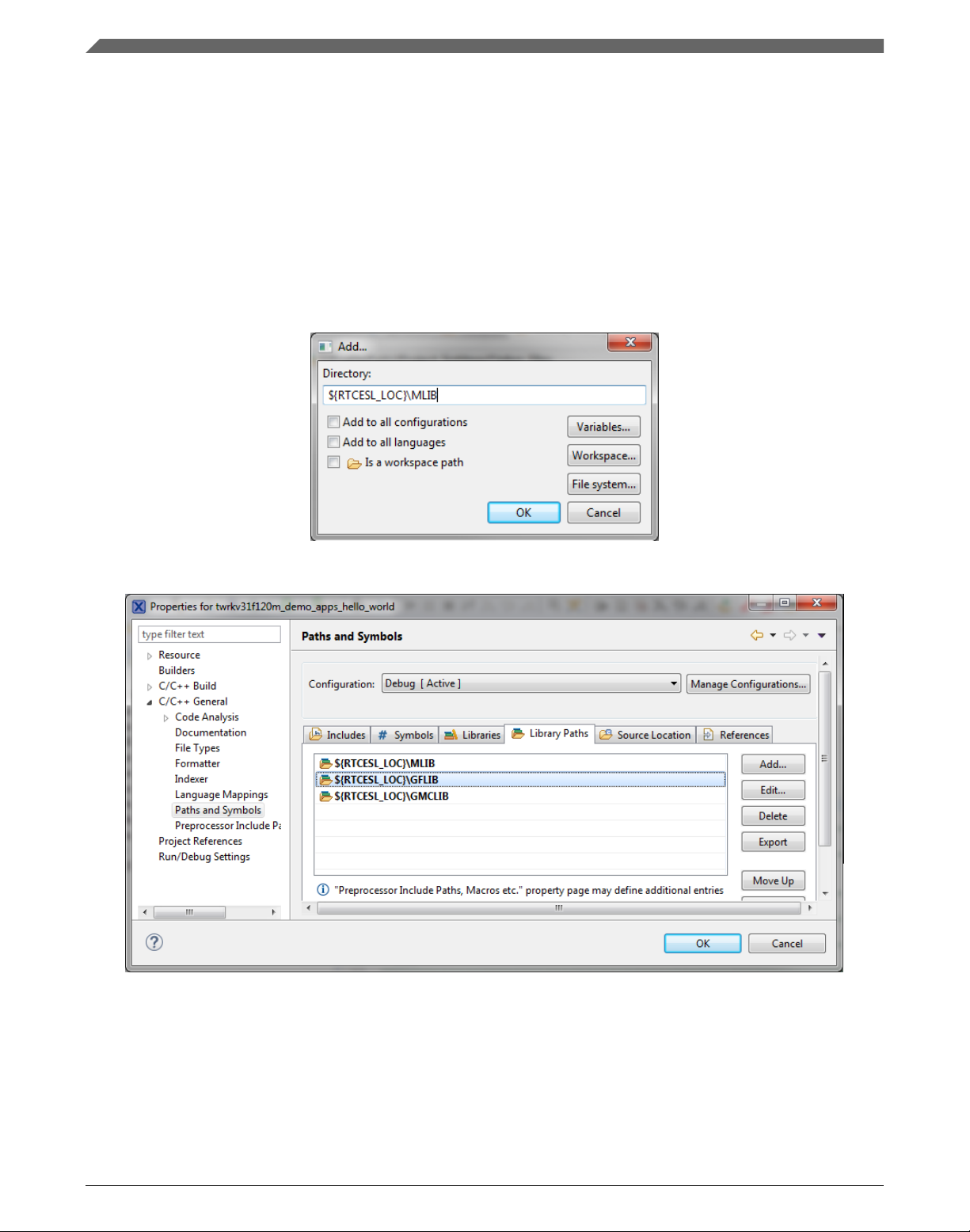
2. Expand the C/C++ General node, and click Paths and Symbols.

3. In the right-hand dialog, select the Library Paths tab. See Figure 1-9.

4. Click the Add… button on the right, and a dialog appears.

GMCLIB User's Guide, Rev. 4, 12/2020

NXP Semiconductors 13

Library integration into project (MCUXpresso IDE)

5. Look for the RTCESL_LOC variable by clicking Variables…, and then finish the path in the box by adding the following (see Figure 1-8): ${RTCESL_LOC}\MLIB.

6. Click OK, and then click the Add… button.

7. Look for the RTCESL_LOC variable by clicking Variables…, and then finish the path in the box by adding the following: ${RTCESL_LOC}\GFLIB.

8. Click OK, and then click the Add… button.

9. Look for the RTCESL_LOC variable by clicking Variables…, and then finish the path in the box by adding the following: ${RTCESL_LOC}\GMCLIB.

10. Click OK, you will see the paths added into the list. See Figure 1-9.

Figure 1-8. Library path inclusion

Figure 1-9. Library paths

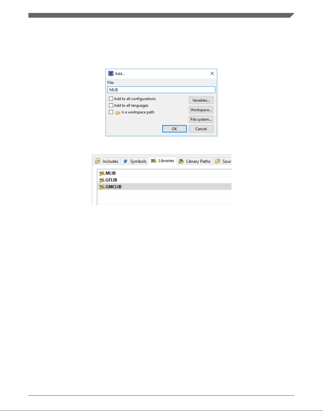
11. After adding the library paths, add the library files. Click the Libraries tab. See

Figure 1-11.

12. Click the Add… button on the right, and a dialog appears.

13. Type the following into the File text box (see Figure 1-10): :mlib.a

14. Click OK, and then click the Add… button.

GMCLIB User's Guide, Rev. 4, 12/2020

14 NXP Semiconductors

Chapter 1 Library

15. Type the following into the File text box: :gflib.a

16. Click OK, and then click the Add… button.

17. Type the following into the File text box: :gmclib.a

18. Click OK, and you will see the libraries added in the list. See Figure 1-11.

Figure 1-10. Library file inclusion

Figure 1-11. Libraries

19. In the right-hand dialog, select the Includes tab, and click GNU C in the Languages list. See Figure 1-13.

20. Click the Add… button on the right, and a dialog appears. See Figure 1-12.

21. Look for the RTCESL_LOC variable by clicking Variables…, and then finish the path in the box to be: ${RTCESL_LOC}\MLIB\Include

22. Click OK, and then click the Add… button.

23. Look for the RTCESL_LOC variable by clicking Variables…, and then finish the path in the box to be: ${RTCESL_LOC}\GFLIB\Include

24. Click OK, and then click the Add… button.

25. Look for the RTCESL_LOC variable by clicking Variables…, and then finish the path in the box to be: ${RTCESL_LOC}\GMCLIB\Include

26. Click OK, and you will see the paths added in the list. See Figure 1-13. Click OK.

GMCLIB User's Guide, Rev. 4, 12/2020

NXP Semiconductors 15

Library integration into project (MCUXpresso IDE)

Figure 1-12. Library include path addition

Figure 1-13. Compiler setting

Type the #include syntax into the code where you want to call the library functions. In the left-hand dialog, open the required .c file. After the file opens, include the following lines into the #include section:

#include "mlib_FP.h" #include "gflib_FP.h" #include "gmclib_FP.h"

When you click the Build icon (hammer), the project is compiled without errors.

GMCLIB User's Guide, Rev. 4, 12/2020

16 NXP Semiconductors

Chapter 1 Library

1.3 Library integration into project (Keil µVision)

This section provides a step-by-step guide on how to quickly and easily include GMCLIB into an empty project or any MCUXpresso SDK example or demo application projects using Keil µVision. This example uses the default installation path (C:\NXP\RTCESL \CM33F_RTCESL_4.6_KEIL). If you have a different installation path, use that path instead. If any MCUXpresso SDK project is intended to use (for example hello_world project) go to Linking the files into the project chapter otherwise read next chapter.

1.3.1

NXP pack installation for new project (without MCUXpresso SDK)

This example uses the NXP LPC55s69 part, and the default installation path (C:\NXP \RTCESL\CM33F_RTCESL_4.6_KEIL) is supposed. If the compiler has never been used to create any NXP MCU-based projects before, check whether the NXP MCU pack for the particular device is installed. Follow these steps:

1. Launch Keil µVision.

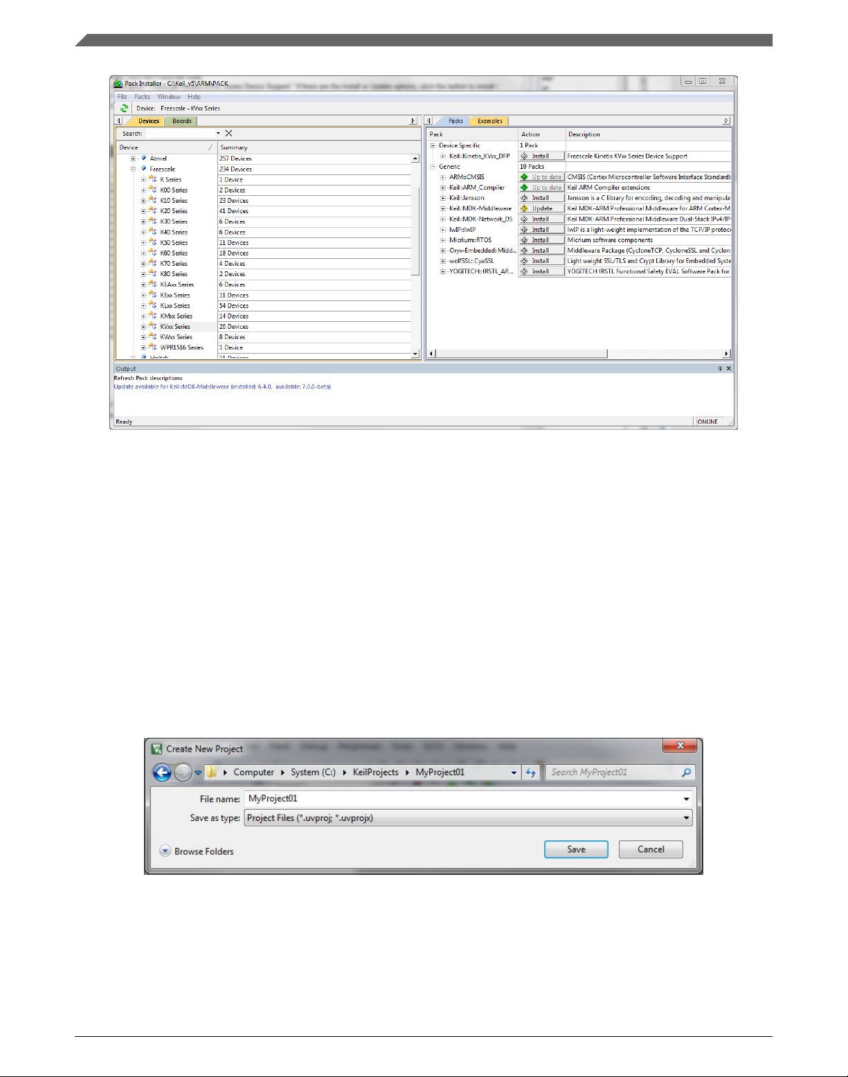
2. In the main menu, go to Project > Manage > Pack Installer….

3. In the left-hand dialog (under the Devices tab), expand the All Devices > Freescale (NXP) node.

4. Look for a line called "KVxx Series" and click it.

5. In the right-hand dialog (under the Packs tab), expand the Device Specific node.

6. Look for a node called "Keil::Kinetis_KVxx_DFP." If there are the Install or Update options, click the button to install/update the package. See Figure 1-14.

7. When installed, the button has the "Up to date" title. Now close the Pack Installer.

GMCLIB User's Guide, Rev. 4, 12/2020

NXP Semiconductors 17

Library integration into project (Keil µVision)

Figure 1-14. Pack Installer

1.3.2

New project (without MCUXpresso SDK)

To start working on an application, create a new project. If the project already exists and is opened, skip to the next section. Follow these steps to create a new project:

1. Launch Keil µVision.

2. In the main menu, select Project > New µVision Project…, and the Create New Project dialog appears.

3. Navigate to the folder where you want to create the project, for example C: \KeilProjects\MyProject01. Type the name of the project, for example MyProject01. Click Save. See Figure 1-15.

Figure 1-15. Create New Project dialog

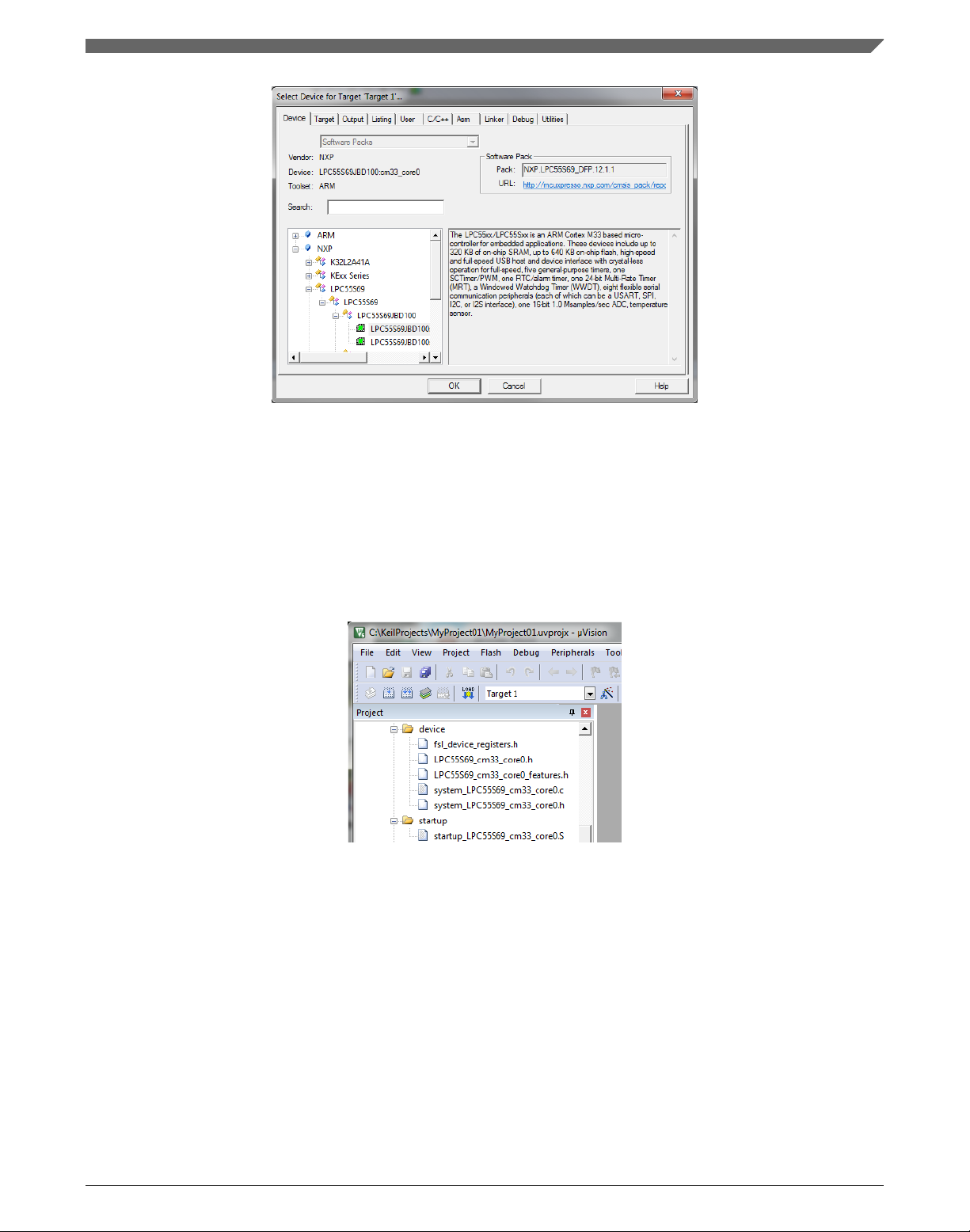
4. In the next dialog, select the Software Packs in the very first box.

5. Type '' into the Search box, so that the device list is reduced to the devices.

6. Expand the node.

7. Click the LPC55s69 node, and then click OK. See Figure 1-16.

GMCLIB User's Guide, Rev. 4, 12/2020

18 NXP Semiconductors

Chapter 1 Library

Figure 1-16. Select Device dialog

8. In the next dialog, expand the Device node, and tick the box next to the Startup node. See Figure 1-17.

9. Expand the CMSIS node, and tick the box next to the CORE node.

Figure 1-17. Manage Run-Time Environment dialog

10. Click OK, and a new project is created. The new project is now visible in the lefthand part of Keil µVision. See Figure 1-18.

Figure 1-18. Project

11. In the main menu, go to Project > Options for Target 'Target1'…, and a dialog appears.

12. Select the Target tab.

13. Select Use Single Precision in the Floating Point Hardware option. See Figure 1-18.

GMCLIB User's Guide, Rev. 4, 12/2020

NXP Semiconductors 19

Library integration into project (Keil µVision)

Figure 1-19. FPU

1.3.3 PowerQuad DSP Coprocessor and Accelerator support

Some LPC platforms (LPC55S6x) contain a hardware accelerator dedicated to common calculations in DSP applications. This section shows how to turn the PowerQuad (PQ) support for a function on and off.

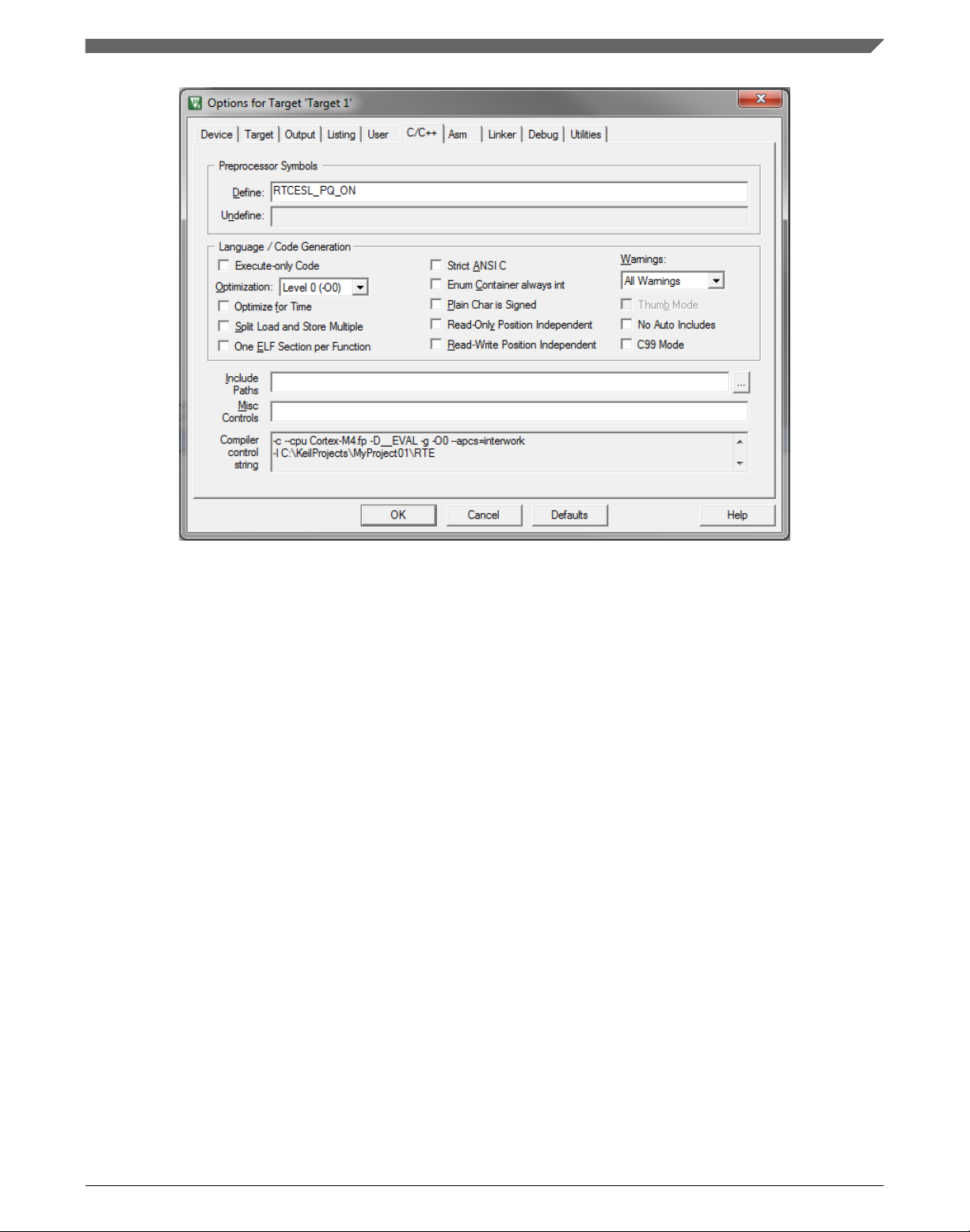
1. In the main menu, go to Project > Options for Target 'Target1'…, and a dialog appears.

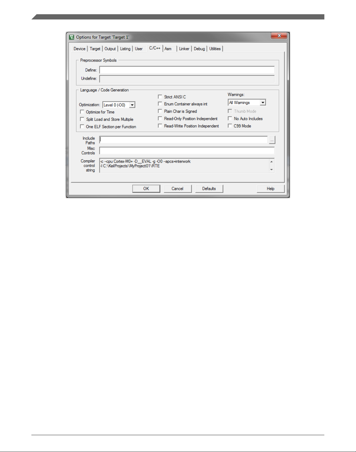
2. Select the C/C++ tab. See Figure 1-20.

3. In the Include Preprocessor Symbols text box, type the following:

• RTCESL_PQ_ON—to turn the hardware division and square root support on.

• RTCESL_PQ_OFF—to turn the hardware division and square root support off.

If neither of these two defines is defined, the hardware division and square root support is turned off by default.

GMCLIB User's Guide, Rev. 4, 12/2020

20 NXP Semiconductors

Chapter 1 Library

Figure 1-20. Preprocessor symbols

4. Click OK in the main dialog.

5. Ensure the PowerQuad moduel to be clocked by calling function RTCESL_PQ_Init(); prior to the first function using PQ module calling.

See the device reference manual to verify whether the device contains the PowerQuad DSP Coprocessor and Accelerator support.

1.3.4

Linking the files into the project

GMCLIB requires MLIB and GFLIB to be included too. The following steps show how to include all dependent modules.

To include the library files in the project, create groups and add them.

1. Right-click the Target 1 node in the left-hand part of the Project tree, and select Add Group… from the menu. A new group with the name New Group is added.

2. Click the newly created group, and press F2 to rename it to RTCESL.

3. Right-click the RTCESL node, and select Add Existing Files to Group 'RTCESL'… from the menu.

GMCLIB User's Guide, Rev. 4, 12/2020

NXP Semiconductors 21

Library integration into project (Keil µVision)

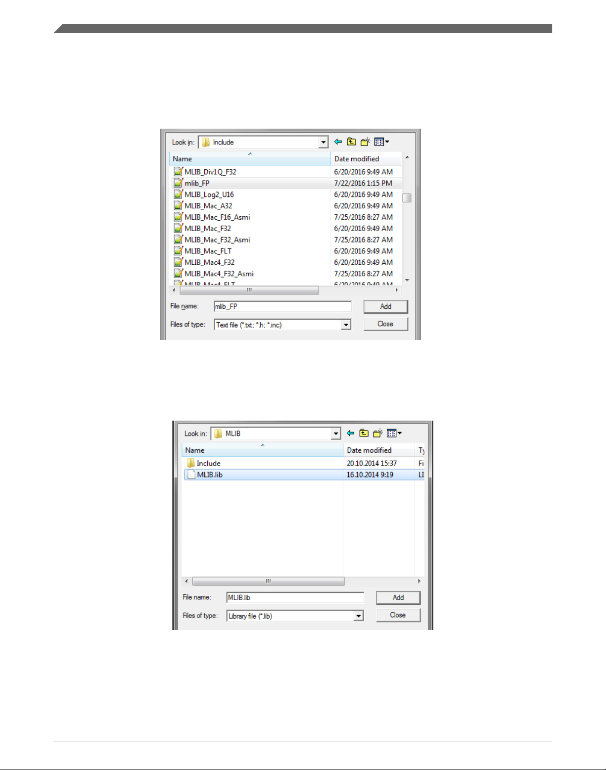
4. Navigate into the library installation folder C:\NXP\RTCESL \CM33F_RTCESL_4.6_KEIL\MLIB\Include, and select the mlib_FP.h file. If the file does not appear, set the Files of type filter to Text file. Click Add. See Figure

1-21.

Figure 1-21. Adding .h files dialog

5. Navigate to the parent folder C:\NXP\RTCESL\CM33F_RTCESL_4.6_KEIL\MLIB, and select the mlib.lib file. If the file does not appear, set the Files of type filter to Library file. Click Add. See Figure 1-22.

Figure 1-22. Adding .lib files dialog

6. Navigate into the library installation folder C:\NXP\RTCESL \CM33F_RTCESL_4.6_KEIL\GFLIB\Include, and select the gflib_FP.h file. If the file does not appear, set the Files of type filter to Text file. Click Add.

GMCLIB User's Guide, Rev. 4, 12/2020

22 NXP Semiconductors

Chapter 1 Library

7. Navigate to the parent folder C:\NXP\RTCESL\CM33F_RTCESL_4.6_KEIL \GFLIB, and select the gflib.lib file. If the file does not appear, set the Files of type filter to Library file. Click Add.

8. Navigate into the library installation folder C:\NXP\RTCESL \CM33F_RTCESL_4.6_KEIL\GMCLIB\Include, and select the gmclib_FP.h file. If the file does not appear, set the Files of type filter to Text file. Click Add.

9. Navigate to the parent folder C:\NXP\RTCESL\CM33F_RTCESL_4.6_KEIL \GMCLIB, and select the gmclib.lib file. If the file does not appear, set the Files of type filter to Library file. Click Add.

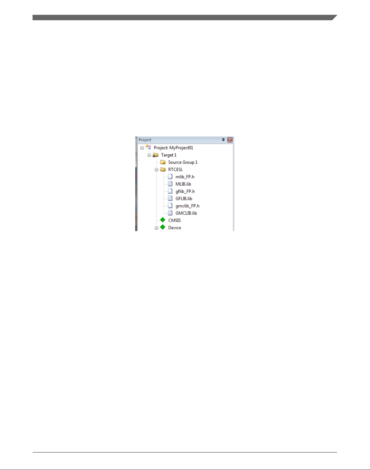
10. Now, all necessary files are in the project tree; see Figure 1-23. Click Close.

Figure 1-23. Project workspace

1.3.5

Library path setup

The following steps show the inclusion of all dependent modules.

1. In the main menu, go to Project > Options for Target 'Target1'…, and a dialog appears.

2. Select the C/C++ tab. See Figure 1-24.

3. In the Include Paths text box, type the following paths (if there are more paths, they must be separated by ';') or add them by clicking the … button next to the text box:

• "C:\NXP\RTCESL\CM33F_RTCESL_4.6_KEIL\MLIB\Include"

• "C:\NXP\RTCESL\CM33F_RTCESL_4.6_KEIL\GFLIB\Include"

• "C:\NXP\RTCESL\CM33F_RTCESL_4.6_KEIL\GMCLIB\Include"

4. Click OK.

5. Click OK in the main dialog.

GMCLIB User's Guide, Rev. 4, 12/2020

NXP Semiconductors 23

Library integration into project (Keil µVision)

Figure 1-24. Library path addition

Type the #include syntax into the code. Include the library into a source file. In the new project, it is necessary to create a source file:

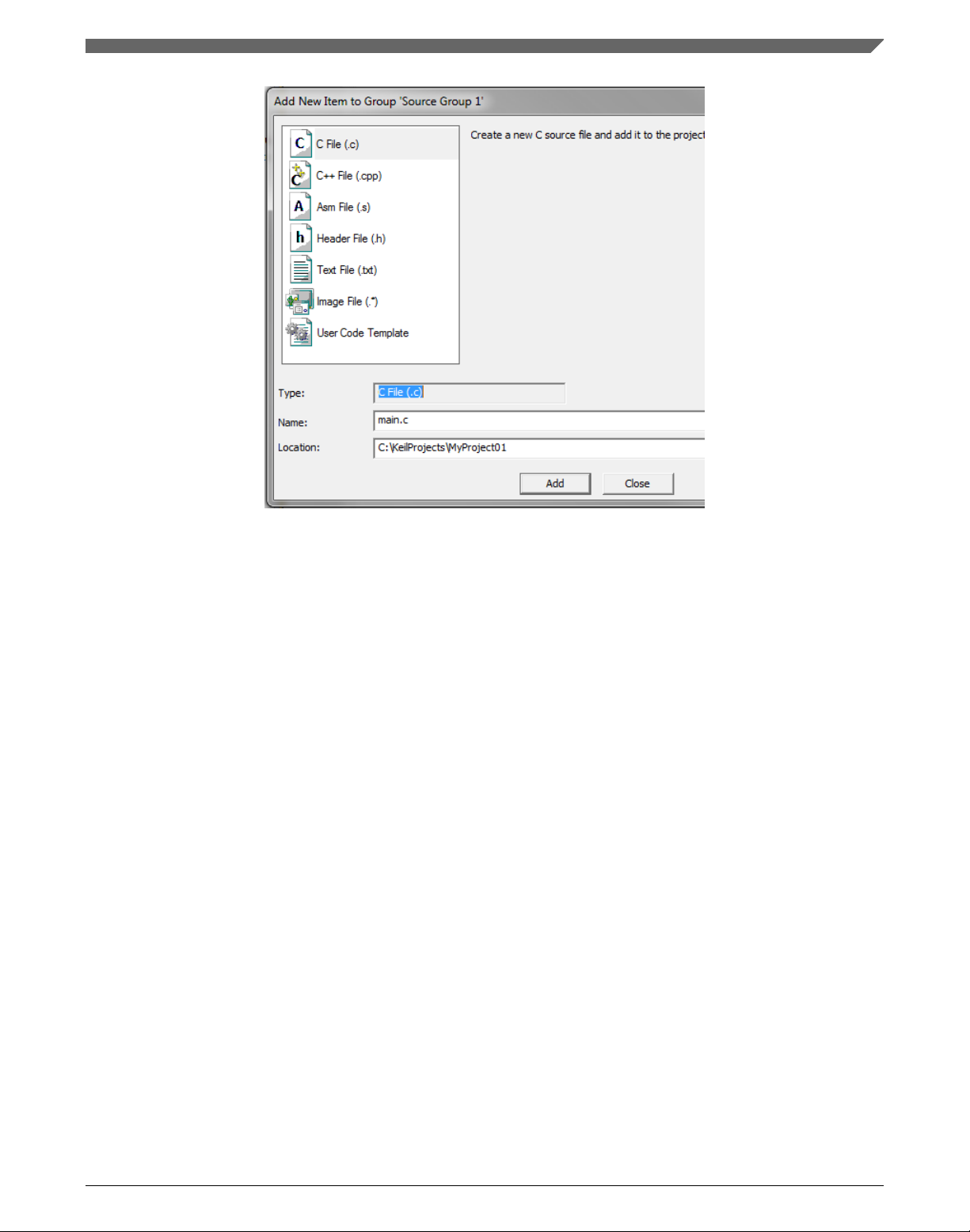
1. Right-click the Source Group 1 node, and Add New Item to Group 'Source Group 1'… from the menu.

Select the C File (.c) option, and type a name of the file into the Name box, for example 'main.c'. See Figure 1-25.

GMCLIB User's Guide, Rev. 4, 12/2020

24 NXP Semiconductors

Chapter 1 Library

Figure 1-25. Adding new source file dialog

3. Click Add, and a new source file is created and opened up.

4. In the opened source file, include the following lines into the #include section, and create a main function:

#include "mlib_FP.h" #include "gflib_FP.h" #include "gmclib_FP.h"

int main(void) { while(1); }

When you click the Build (F7) icon, the project will be compiled without errors.

1.4

Library integration into project (IAR Embedded Workbench)

This section provides a step-by-step guide on how to quickly and easily include the GMCLIB into an empty project or any MCUXpresso SDK example or demo application projects using IAR Embedded Workbench. This example uses the default installation path (C:\NXP\RTCESL\CM33F_RTCESL_4.6_IAR). If you have a different installation path, use that path instead. If any MCUXpresso SDK project is intended to use (for example hello_world project) go to Linking the files into the project chapter otherwise read next chapter.

GMCLIB User's Guide, Rev. 4, 12/2020

NXP Semiconductors 25

Library integration into project (IAR Embedded Workbench)

1.4.1 New project (without MCUXpresso SDK)

This example uses the NXP LPC55S69 part, and the default installation path (C:\NXP \RTCESL\CM33F_RTCESL_4.6_IAR) is supposed. To start working on an application, create a new project. If the project already exists and is opened, skip to the next section. Perform these steps to create a new project:

1. Launch IAR Embedded Workbench.

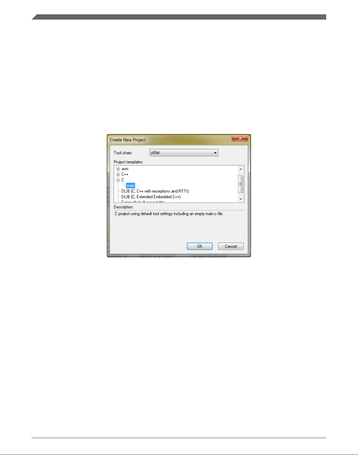
2. In the main menu, select Project > Create New Project… so that the "Create New Project" dialog appears. See Figure 1-26.

Figure 1-26. Create New Project dialog

3. Expand the C node in the tree, and select the "main" node. Click OK.

4. Navigate to the folder where you want to create the project, for example, C: \IARProjects\MyProject01. Type the name of the project, for example, MyProject01. Click Save, and a new project is created. The new project is now visible in the lefthand part of IAR Embedded Workbench. See Figure 1-27.

GMCLIB User's Guide, Rev. 4, 12/2020

26 NXP Semiconductors

Chapter 1 Library

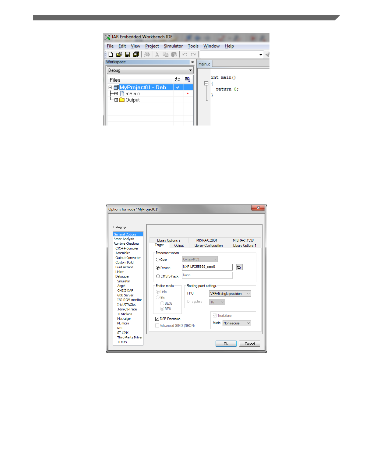
Figure 1-27. New project

5. In the main menu, go to Project > Options…, and a dialog appears.

6. In the Target tab, select the Device option, and click the button next to the dialog to select the MCU. In this example, select NXP > LPC55S69 > NXP LPC55S69_core0. Select VFPv5 single precision in the FPU option.The DSP instructions group is required please check the DSP Extensions checkbox if not checked. Click OK. See

Figure 1-28.

Figure 1-28. Options dialog

GMCLIB User's Guide, Rev. 4, 12/2020

NXP Semiconductors 27

Library integration into project (IAR Embedded Workbench)

1.4.2 PowerQuad DSP Coprocessor and Accelerator support

Some LPC platforms (LPC55S6x) contain a hardware accelerator dedicated to common calculations in DSP applications. Only functions runing faster through the PowerQuad module than the core itself are supported and targeted to be calculated by the PowerQuad module. This section shows how to turn the PowerQuad (PQ) support for a function on and off.

1. In the main menu, go to Project > Options…, and a dialog appears.

2. In the left-hand column, select C/C++ Compiler.

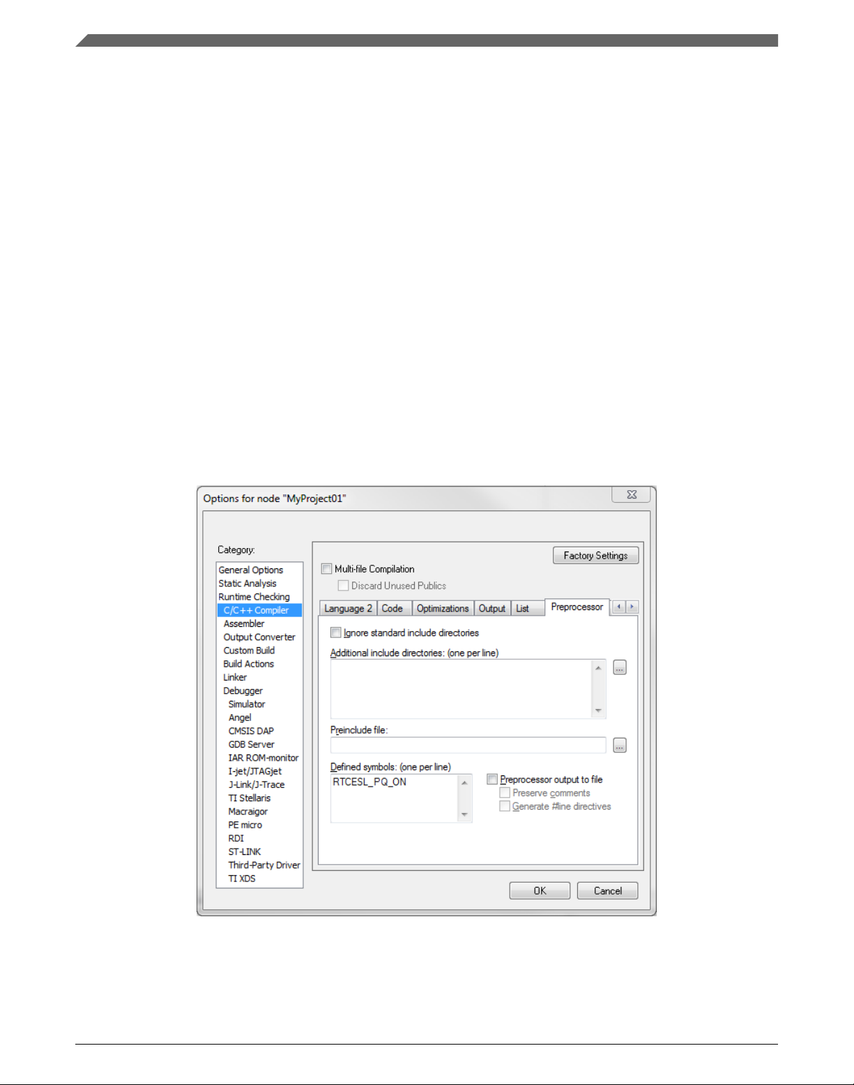
3. In the right-hand part of the dialog, click the Preprocessor tab (it can be hidden in the right-hand side; use the arrow icons for navigation).

4. In the text box (at the Defined symbols: (one per line)), type the following (See

Figure 1-29):

• RTCESL_PQ_ON—to turn the PowerQuad support on.

• RTCESL_PQ_OFF—to turn the PowerQuad support off.

If neither of these two defines is defined, the hardware division and square root support is turned off by default.

Figure 1-29. Defined symbols

5. Click OK in the main dialog.

GMCLIB User's Guide, Rev. 4, 12/2020

28 NXP Semiconductors

Chapter 1 Library

6. Ensure the PowerQuad moduel to be clocked by calling function RTCESL_PQ_Init(); prior to the first function using PQ module calling.

See the device reference manual to verify whether the device contains the PowerQuad DSP Coprocessor and Accelerator support.

1.4.3 Library path variable

To make the library integration easier, create a variable that will hold the information about the library path.

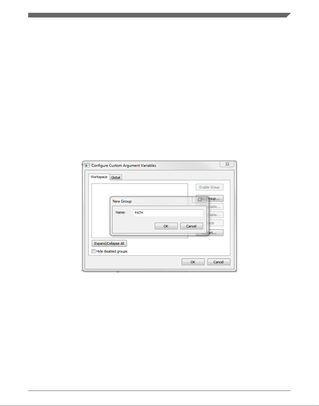
1. In the main menu, go to Tools > Configure Custom Argument Variables…, and a dialog appears.

2. Click the New Group button, and another dialog appears. In this dialog, type the name of the group PATH, and click OK. See Figure 1-30.

Figure 1-30. New Group

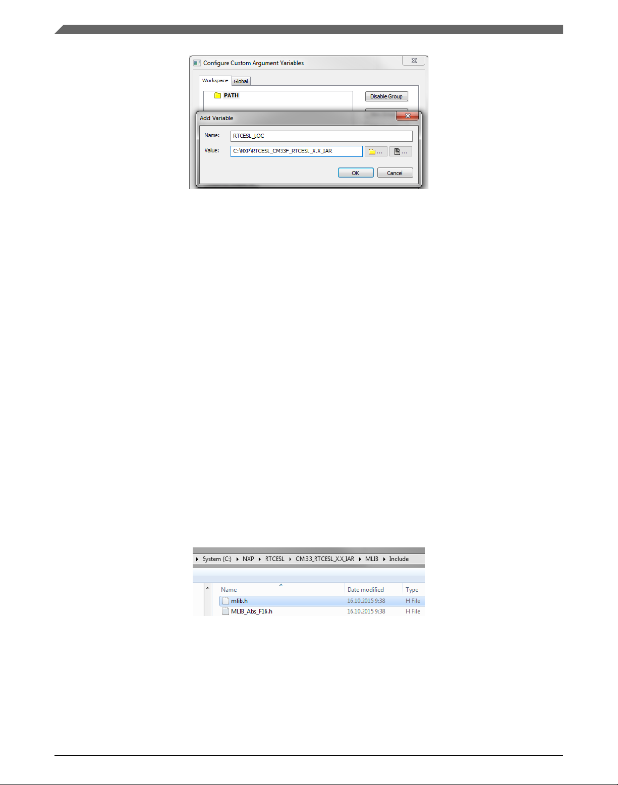
3. Click on the newly created group, and click the Add Variable button. A dialog appears.

4. Type this name: RTCESL_LOC

5. To set up the value, look for the library by clicking the '…' button, or just type the installation path into the box: C:\NXP\RTCESL\CM33F_RTCESL_4.6_IAR. Click OK.

6. In the main dialog, click OK. See Figure 1-31.

GMCLIB User's Guide, Rev. 4, 12/2020

NXP Semiconductors 29

Library integration into project (IAR Embedded Workbench)

Figure 1-31. New variable

1.4.4

Linking the files into the project

GMCLIB requires MLIB and GFLIB to be included too. The following steps show the inclusion of all dependent modules.

To include the library files into the project, create groups and add them.

1. Go to the main menu Project > Add Group…

2. Type RTCESL, and click OK.

3. Click on the newly created node RTCESL, go to Project > Add Group…, and create a MLIB subgroup.

4. Click on the newly created node MLIB, and go to the main menu Project > Add Files… See Figure 1-33.

5. Navigate into the library installation folder C:\NXP\RTCESL \CM33F_RTCESL_4.6_IAR\MLIB\Include, and select the mlib.h file. (If the file does not appear, set the file-type filter to Source Files.) Click Open. See Figure 1-32.

6. Navigate into the library installation folder C:\NXP\RTCESL \CM33F_RTCESL_4.6_IAR\MLIB, and select the mlib.a file. If the file does not appear, set the file-type filter to Library / Object files. Click Open.

Figure 1-32. Add Files dialog

7. Click on the RTCESL node, go to Project > Add Group…, and create a GFLIB subgroup.

8. Click on the newly created node GFLIB, and go to the main menu Project > Add Files….

GMCLIB User's Guide, Rev. 4, 12/2020

30 NXP Semiconductors

Chapter 1 Library

9. Navigate into the library installation folder C:\NXP\RTCESL \CM33F_RTCESL_4.6_IAR\GFLIB\Include, and select the gflib.h file. (If the file does not appear, set the file-type filter to Source Files.) Click Open.

10. Navigate into the library installation folder C:\NXP\RTCESL \CM33F_RTCESL_4.6_IAR\GFLIB, and select the gflib.a file. If the file does not appear, set the file-type filter to Library / Object files. Click Open.

11. Click on the RTCESL node, go to Project > Add Group…, and create a GMCLIB subgroup.

12. Click on the newly created node GMCLIB, and go to the main menu Project > Add Files….

13. Navigate into the library installation folder C:\NXP\RTCESL \CM33F_RTCESL_4.6_IAR\GMCLIB\Include, and select the gmclib.h file. If the file does not appear, set the file-type filter to Source Files. Click Open.

14. Navigate into the library installation folder C:\NXP\RTCESL \CM33F_RTCESL_4.6_IAR\GMCLIB, and select the gmclib.a file. If the file does not appear, set the file-type filter to Library / Object files. Click Open.

15. Now you will see the files added in the workspace. See Figure 1-33.

Figure 1-33. Project workspace

1.4.5

Library path setup

The following steps show the inclusion of all dependent modules:

1. In the main menu, go to Project > Options…, and a dialog appears.

2. In the left-hand column, select C/C++ Compiler.

3. In the right-hand part of the dialog, click on the Preprocessor tab (it can be hidden in the right; use the arrow icons for navigation).

4. In the text box (at the Additional include directories title), type the following folder (using the created variable):

GMCLIB User's Guide, Rev. 4, 12/2020

NXP Semiconductors 31

Library integration into project (IAR Embedded Workbench)

• $RTCESL_LOC$\MLIB\Include

• $RTCESL_LOC$\GFLIB\Include

• $RTCESL_LOC$\GMCLIB\Include

5. Click OK in the main dialog. See Figure 1-34.

Figure 1-34. Library path adition

Type the #include syntax into the code. Include the library included into the main.c file. In the workspace tree, double-click the main.c file. After the main.c file opens up, include the following lines into the #include section:

#include "mlib_FP.h" #include "gflib_FP.h" #include "gmclib_FP.h"

When you click the Make icon, the project will be compiled without errors.

GMCLIB User's Guide, Rev. 4, 12/2020

32 NXP Semiconductors

Chapter 2 Algorithms in detail

2.1 GMCLIB_Clark

The

GMCLIB_Clark function calculates the Clarke transformation, which is used to

transform values (flux, voltage, current) from the three-phase coordinate system to the two-phase (α-β) orthogonal coordinate system, according to the following equations:

Equation 1

Equation 2

2.1.1

Available versions

This function is available in the following versions:

• Fractional output - the output is the fractional portion of the result; the result is within the range <-1 ; 1). The result may saturate.

• Floating-point output - the output is the floating-point result within the type's full range.

The available versions of the GMCLIB_Clark function are shown in the following table:

Table 2-1. Function versions

Function name Input type Output type Result type

GMCLIB_Clark_F16 GMCLIB_3COOR_T_F16 * GMCLIB_2COOR_ALBE_T_F16 * void

Clarke transformation of a 16-bit fractional three-phase system input to a 16-bit fractional twophase system. The input and output are within the fractional range <-1 ; 1).

GMCLIB_Clark_FLT GMCLIB_3COOR_T_FLT * GMCLIB_2COOR_ALBE_T_FLT * void

Table continues on the next page...

GMCLIB User's Guide, Rev. 4, 12/2020

NXP Semiconductors 33

GMCLIB_Clark

Table 2-1. Function versions (continued)

Function name Input type Output type Result type

Clarke transformation of a 32-bit single precision floating-point three-phase system input to a 32bit single-point floating-point two-phase system. The input and output are within the full 32-bit single-point floating-point range.

2.1.2 Declaration

The available GMCLIB_Clark functions have the following declarations:

void GMCLIB_Clark_F16(const GMCLIB_3COOR_T_F16 *psIn, GMCLIB_2COOR_ALBE_T_F16 *psOut) void GMCLIB_Clark_FLT(const GMCLIB_3COOR_T_FLT *psIn, GMCLIB_2COOR_ALBE_T_FLT *psOut)

2.1.3

Function use

The use of the GMCLIB_Clark function is shown in the following examples:

Fixed-point version:

#include "gmclib.h"

static GMCLIB_2COOR_ALBE_T_F16 sAlphaBeta; static GMCLIB_3COOR_T_F16 sAbc;

void Isr(void);

void main(void) { /* ABC structure initialization */ sAbc.f16A = FRAC16(0.0); sAbc.f16B = FRAC16(0.0); sAbc.f16C = FRAC16(0.0); }

/* Periodical function or interrupt */ void Isr(void) { /* Clarke Transformation calculation */ GMCLIB_Clark_F16(&sAbc, &sAlphaBeta); }

Floating-point version:

#include "gmclib.h"

static GMCLIB_2COOR_ALBE_T_FLT sAlphaBeta; static GMCLIB_3COOR_T_FLT sAbc;

void Isr(void);

GMCLIB User's Guide, Rev. 4, 12/2020

34 NXP Semiconductors

Chapter 2 Algorithms in detail

void main(void) { /* ABC structure initialization */ sAbc.fltA = 0.0F; sAbc.fltB = 0.0F; sAbc.fltC = 0.0F; }

/* Periodical function or interrupt */ void Isr(void) { /* Clarke Transformation calculation */ GMCLIB_Clark_FLT(&sAbc, &sAlphaBeta); }

2.2 GMCLIB_ClarkInv

The

GMCLIB_ClarkInv function calculates the Clarke transformation, which is used to

transform values (flux, voltage, current) from the two-phase (α-β) orthogonal coordinate system to the three-phase coordinate system, according to the following equations:

Equation 3

Equation 4

Equation 5

2.2.1

Available versions

This function is available in the following versions:

• Fractional output - the output is the fractional portion of the result; the result is within the range <-1 ; 1). The result may saturate.

• Floating-point output - the output is the floating-point result within the type's full range.

GMCLIB User's Guide, Rev. 4, 12/2020

NXP Semiconductors 35

GMCLIB_ClarkInv

The available versions of the GMCLIB_ClarkInv function are shown in the following table:

Table 2-2. Function versions

Function name Input type Output type Result type

GMCLIB_ClarkInv_F16 GMCLIB_2COOR_ALBE_T_F16 * GMCLIB_3COOR_T_F16 * void

Inverse Clarke transformation with a 16-bit fractional two-phase system input and a 16-bit fractional three-phase output. The input and output are within the fractional range <-1 ; 1).

GMCLIB_ClarkInv_FLT GMCLIB_2COOR_ALBE_T_FLT * GMCLIB_3COOR_T_FLT * void

Inverse Clarke transformation with a 32-bit single precision floating-point two-phase system input and a 32-bit single precision floating-point three-phase output. The input and output are within the full 32-bit single-point floating-point range.

2.2.2 Declaration

The available GMCLIB_ClarkInv functions have the following declarations:

void GMCLIB_ClarkInv_F16(const GMCLIB_2COOR_ALBE_T_F16 *psIn, GMCLIB_3COOR_T_F16 *psOut) void GMCLIB_ClarkInv_FLT(const GMCLIB_2COOR_ALBE_T_FLT *psIn, GMCLIB_3COOR_T_FLT *psOut)

2.2.3

Function use

The use of the GMCLIB_ClarkInv function is shown in the following examples:

Fixed-point version:

#include "gmclib.h"

static GMCLIB_2COOR_ALBE_T_F16 sAlphaBeta; static GMCLIB_3COOR_T_F16 sAbc;

void Isr(void);

void main(void) { /* Alpha, Beta structure initialization */ sAlphaBeta.f16Alpha = FRAC16(0.0); sAlphaBeta.f16Beta = FRAC16(0.0); }

/* Periodical function or interrupt */ void Isr(void) { /* Inverse Clarke Transformation calculation */ GMCLIB_ClarkInv_F16(&sAlphaBeta, &sAbc); }

GMCLIB User's Guide, Rev. 4, 12/2020

36 NXP Semiconductors

Floating-point version:

#include "gmclib.h"

static GMCLIB_2COOR_ALBE_T_FLT sAlphaBeta; static GMCLIB_3COOR_T_FLT sAbc;

void Isr(void);

void main(void) { /* Alpha, Beta structure initialization */ sAlphaBeta.fltAlpha = 0.0F; sAlphaBeta.fltBeta = 0.0F; }

/* Periodical function or interrupt */ void Isr(void) { /* Inverse Clarke Transformation calculation */ GMCLIB_ClarkInv_FLT(&sAlphaBeta, &sAbc); }

Chapter 2 Algorithms in detail

2.3

GMCLIB_Park

The GMCLIB_Park function calculates the Park transformation, which transforms values (flux, voltage, current) from the stationary two-phase (α-β) orthogonal coordinate system to the rotating two-phase (d-q) orthogonal coordinate system, according to the following equations:

Equation 6

Equation 7

where:

• θ is the position (angle)

2.3.1

Available versions

This function is available in the following versions:

• Fractional output - the output is the fractional portion of the result; the result is within the range <-1 ; 1). The result may saturate.

• Floating-point output - the output is the floating-point result within the type's full range.

GMCLIB User's Guide, Rev. 4, 12/2020

NXP Semiconductors 37

GMCLIB_Park

The available versions of the GMCLIB_Park function are shown in the following table:

Table 2-3. Function versions

Function name Input type Output type Result type

GMCLIB_Park_F16 GMCLIB_2COOR_ALBE_T_F16 * GMCLIB_2COOR_DQ_T_F16 * void

GMCLIB_2COOR_SINCOS_T_F16 *

The Park transformation of a 16-bit fractional two-phase stationary system input to a 16-bit fractional two-phase rotating system, using a 16-bit fractional angle two-component (sin / cos) position information. The inputs and the output are within the fractional range <-1 ; 1).

GMCLIB_Park_FLT GMCLIB_2COOR_ALBE_T_FLT * GMCLIB_2COOR_DQ_T_FLT * void

GMCLIB_2COOR_SINCOS_T_FLT *

The Park transformation of a 32-bit single precision floating-point two-phase stationary system input to a 32-bit single precision floating-point two-phase rotating system, using a 32-bit single precision floating-point angle two-component (sin / cos) position information. The two-phase stationary system input and the output are within the full 32-bit single-point floating-point range; the angle input is within the range <-1.0 ; 1.0>.

2.3.2 Declaration

The available GMCLIB_Park functions have the following declarations:

void GMCLIB_Park_F16(const GMCLIB_2COOR_ALBE_T_F16 *psIn, const GMCLIB_2COOR_SINCOS_T_F16 *psAnglePos, GMCLIB_2COOR_DQ_T_F16 *psOut)

void GMCLIB_Park_FLT(const GMCLIB_2COOR_ALBE_T_FLT *psIn, const GMCLIB_2COOR_SINCOS_T_FLT *psAnglePos, GMCLIB_2COOR_DQ_T_FLT *psOut)

2.3.3

The use of the GMCLIB_Park function is shown in the following examples:

Fixed-point version:

#include "gmclib.h"

static GMCLIB_2COOR_ALBE_T_F16 sAlphaBeta; static GMCLIB_2COOR_DQ_T_F16 sDQ; static GMCLIB_2COOR_SINCOS_T_F16 sAngle;

Function use

void Isr(void);

void main(void) { /* Alpha, Beta structure initialization */ sAlphaBeta.f16Alpha = FRAC16(0.0); sAlphaBeta.f16Beta = FRAC16(0.0);

GMCLIB User's Guide, Rev. 4, 12/2020

38 NXP Semiconductors

/* Angle structure initialization */ sAngle.f16Sin = FRAC16(0.0); sAngle.f16Cos = FRAC16(1.0); }

/* Periodical function or interrupt */ void Isr(void) { /* Park Transformation calculation */ GMCLIB_Park_F16(&sAlphaBeta, &sAngle, &sDQ); }

Floating-point version:

#include "gmclib.h"

static GMCLIB_2COOR_ALBE_T_FLT sAlphaBeta; static GMCLIB_2COOR_DQ_T_FLT sDQ; static GMCLIB_2COOR_SINCOS_T_FLT sAngle;

void Isr(void);

void main(void) { /* Alpha, Beta structure initialization */ sAlphaBeta.fltAlpha = 0.0F; sAlphaBeta.fltBeta = 0.0F;

/* Angle structure initialization */ sAngle.fltSin = 0.0F; sAngle.fltCos = 1.0F; }

Chapter 2 Algorithms in detail

/* Periodical function or interrupt */ void Isr(void) { /* Park Transformation calculation */ GMCLIB_Park_FLT(&sAlphaBeta, &sAngle, &sDQ); }

2.4

GMCLIB_ParkInv

The GMCLIB_ParkInv function calculates the Park transformation, which transforms values (flux, voltage, current) from the rotating two-phase (d-q) orthogonal coordinate system to the stationary two-phase (α-β) coordinate system, according to the following equations:

Equation 8

Equation 9

where:

GMCLIB User's Guide, Rev. 4, 12/2020

NXP Semiconductors 39

GMCLIB_ParkInv

• θ is the position (angle)

2.4.1 Available versions

This function is available in the following versions:

• Fractional output - the output is the fractional portion of the result; the result is within the range <-1 ; 1). The result may saturate.

• Floating-point output - the output is the floating-point result within the type's full range.

The available versions of the GMCLIB_ParkInv function are shown in the following table:

Table 2-4. Function versions

Function name Input type Output type Result type

GMCLIB_ParkInv_F16 GMCLIB_2COOR_DQ_T_F16 * GMCLIB_2COOR_ALBE_T_F16 * void

GMCLIB_2COOR_SINCOS_T_F16 *

Inverse Park transformation of a 16-bit fractional two-phase rotating system input to a 16-bit fractional two-phase stationary system, using a 16-bit fractional angle two-component (sin / cos) position information. The inputs and the output are within the fractional range <-1 ; 1).

GMCLIB_ParkInv_FLT GMCLIB_2COOR_DQ_T_FLT * GMCLIB_2COOR_ALBE_T_FLT * void

GMCLIB_2COOR_SINCOS_T_FLT *

Inverse Park transformation of a 32-bit single precision floating-point two-phase rotating system input to a 32-bit single precision floating-point two-phase stationary system, using a 32-bit single precision floating-point angle two-component (sin / cos) position information. The two-phase rotating system input and the output are within the full 32-bit single-point floating-point range; the angle input is within the range <-1.0 ; 1.0> .

2.4.2 Declaration

The available GMCLIB_ParkInv functions have the following declarations:

void GMCLIB_ParkInv_F16(const GMCLIB_2COOR_DQ_T_F16 *psIn, const GMCLIB_2COOR_SINCOS_T_F16 *psAnglePos, GMCLIB_2COOR_ALBE_T_F16 *psOut)

void GMCLIB_ParkInv_FLT(const GMCLIB_2COOR_DQ_T_FLT *psIn, const GMCLIB_2COOR_SINCOS_T_FLT *psAnglePos, GMCLIB_2COOR_ALBE_T_FLT *psOut)

2.4.3

The use of the GMCLIB_ParkInv function is shown in the following examples:

40 NXP Semiconductors

Function use

GMCLIB User's Guide, Rev. 4, 12/2020

Fixed-point version:

#include "gmclib.h"

static GMCLIB_2COOR_ALBE_T_F16 sAlphaBeta; static GMCLIB_2COOR_DQ_T_F16 sDQ; static GMCLIB_2COOR_SINCOS_T_F16 sAngle;

void Isr(void);

void main(void) { /* D, Q structure initialization */ sDQ.f16D = FRAC16(0.0); sDQ.f16Q = FRAC16(0.0);

/* Angle structure initialization */ sAngle.f16Sin = FRAC16(0.0); sAngle.f16Cos = FRAC16(1.0); }

/* Periodical function or interrupt */ void Isr(void) { /* Inverse Park Transformation calculation */ GMCLIB_ParkInv_F16(&sDQ, &sAngle, &sAlphaBeta); }

Chapter 2 Algorithms in detail

Floating-point version:

#include "gmclib.h"

static GMCLIB_2COOR_ALBE_T_FLT sAlphaBeta; static GMCLIB_2COOR_DQ_T_FLT sDQ; static GMCLIB_2COOR_SINCOS_T_FLT sAngle;

void Isr(void);

void main(void) { /* D, Q structure initialization */ sDQ.fltD = 0.0F; sDQ.fltQ = 0.0F;

/* Angle structure initialization */ sAngle.fltSin = 0.0F; sAngle.fltCos = 1.0F; }

/* Periodical function or interrupt */ void Isr(void) { /* Inverse Park Transformation calculation */ GMCLIB_ParkInv_FLT(&sDQ, &sAngle, &sAlphaBeta); }

2.5

GMCLIB_DecouplingPMSM

GMCLIB User's Guide, Rev. 4, 12/2020

NXP Semiconductors 41

GMCLIB_DecouplingPMSM

The GMCLIB_DecouplingPMSM function calculates the cross-coupling voltages to eliminate the d-q axis coupling that causes nonlinearity of the control.

The d-q model of the motor contains cross-coupling voltage that causes nonlinearity of the control. Figure 2-1 represents the d-q model of the motor that can be described using the following equations, where the underlined portion is the cross-coupling voltage:

Equation 10

where:

• ud, uq are the d and q voltages

• id, iq are the d and q currents

• Rs is the stator winding resistance

• Ld, Lq are the stator winding d and q inductances

• ωel is the electrical angular speed

• ψr is the rotor flux constant

Figure 2-1. The d-q PMSM model

To eliminate the nonlinearity, the cross-coupling voltage is calculated using the

GMCLIB_DecouplingPMSM algorithm, and feedforwarded to the d and q voltages. The

decoupling algorithm is calculated using the following equations:

GMCLIB User's Guide, Rev. 4, 12/2020

42 NXP Semiconductors

Chapter 2 Algorithms in detail

Equation 11

where:

• ud, uq are the d and q voltages; inputs to the algorithm

• u

ddec

, u

are the d and q decoupled voltages; outputs from the algorithm

qdec

The fractional representation of the d-component equation is as follows:

Equation 12

The fractional representation of the q-component equation is as follows:

Equation 13

where:

• kd, kq are the scaling coefficients

• i

• u

• ω

is the maximum current

max

is the maximum voltage

max

el_max

is the maximum electrical speed

The kd and kq parameters must be set up properly. The principle of the algorithm is depicted in Figure 2-2 :

GMCLIB User's Guide, Rev. 4, 12/2020

NXP Semiconductors 43

GMCLIB_DecouplingPMSM

Figure 2-2. Algorithm diagram

2.5.1

Available versions

This function is available in the following versions:

• Fractional output - the output is the fractional portion of the result; the result is within the range <-1 ; 1). The result may saturate. The parameters use the accumulator types.

• Floating-point output - the output is the floating-point result within the type's full range.

The available versions of the GMCLIB_DecouplingPMSM function are shown in the following table:

Table 2-5. Function versions

Function name Input/output type Result type

GMCLIB_DecouplingPMSM_F16

Input

Parameters Output

GMCLIB_2COOR_DQ_T_F16 * void GMCLIB_2COOR_DQ_T_F16 * frac16_t GMCLIB_DECOUPLINGPMSM_T_A32 * GMCLIB_2COOR_DQ_T_F16 *

Table continues on the next page...

GMCLIB User's Guide, Rev. 4, 12/2020

44 NXP Semiconductors

Function name Input/output type Result type

GMCLIB_DecouplingPMSM_FLT

Chapter 2 Algorithms in detail

Table 2-5. Function versions (continued)

The PMSM decoupling with a 16-bit fractional d-q voltage, current inputs, and a 16bit fractional electrical speed input. The parameters are 32-bit accumulator types. The output is a 16-bit fractional decoupled d-q voltage. The inputs and the output are within the range <-1 ; 1).

Input

Parameters Output

The PMSM decoupling with a 32-bit single precision floating-point d-q voltage, current, and electrical speed input. The parameters are 32-bit single precision floating-point types. The output is a 32-bit single precision floating-point decoupled dq voltage. The inputs and the output are within the full 32-bit single-point floatingpoint range.

GMCLIB_2COOR_DQ_T_FLT * void GMCLIB_2COOR_DQ_T_FLT * float_t GMCLIB_DECOUPLINGPMSM_T_FLT * GMCLIB_2COOR_DQ_T_FLT *

2.5.2 GMCLIB_DECOUPLINGPMSM_T_A32 type description

Variable name Input type Description

a32KdGain acc32_t Direct axis decoupling parameter. The parameter is within the range <0 ; 65536.0) a32KqGain acc32_t Quadrature axis decoupling parameter. The parameter is within the range <0 ;

65536.0)

2.5.3 GMCLIB_DECOUPLINGPMSM_T_FLT type description

Variable name Input type Description

fltLd float_t Direct axis inductance parameter. The parameter is a nonnegative value. fltLq float_t Quadrature axis inductance parameter. The parameter is a nonnegative value.

2.5.4 Declaration

The available GMCLIB_DecouplingPMSM functions have the following declarations:

void GMCLIB_DecouplingPMSM_F16(const GMCLIB_2COOR_DQ_T_F16 *psUDQ, const

GMCLIB_2COOR_DQ_T_F16 *psIDQ, frac16_t f16SpeedEl, const GMCLIB_DECOUPLINGPMSM_T_A32

*psParam, GMCLIB_2COOR_DQ_T_F16 *psUDQDec)

void GMCLIB_DecouplingPMSM_FLT(const GMCLIB_2COOR_DQ_T_FLT *psUDQ, const

GMCLIB User's Guide, Rev. 4, 12/2020

NXP Semiconductors 45

GMCLIB_DecouplingPMSM

GMCLIB_2COOR_DQ_T_FLT *psIDQ, float_t fltSpeedEl, const GMCLIB_DECOUPLINGPMSM_T_FLT

*psParam, GMCLIB_2COOR_DQ_T_FLT *psUDQDec)

2.5.5 Function use

The use of the GMCLIB_DecouplingPMSM function is shown in the following examples:

Fixed-point version:

#include "gmclib.h"

static GMCLIB_2COOR_DQ_T_F16 sVoltageDQ; static GMCLIB_2COOR_DQ_T_F16 sCurrentDQ; static frac16_t f16AngularSpeed; static GMCLIB_DECOUPLINGPMSM_T_A32 sDecouplingParam; static GMCLIB_2COOR_DQ_T_F16 sVoltageDQDecoupled;

void Isr(void);

void main(void) { /* Voltage D, Q structure initialization */ sVoltageDQ.f16D = FRAC16(0.0); sVoltageDQ.f16Q = FRAC16(0.0);

/* Current D, Q structure initialization */ sCurrentDQ.f16D = FRAC16(0.0); sCurrentDQ.f16Q = FRAC16(0.0);

/* Speed initialization */ f16AngularSpeed = FRAC16(0.0);

/* Motor parameters for decoupling Kd = 40, Kq = 20 */ sDecouplingParam.a32KdGain = ACC32(40.0); sDecouplingParam.a32KqGain = ACC32(20.0); }

/* Periodical function or interrupt */ void Isr(void) { /* Decoupling calculation */ GMCLIB_DecouplingPMSM_F16(&sVoltageDQ, &sCurrentDQ, f16AngularSpeed, &sDecouplingParam, &sVoltageDQDecoupled); }

Floating-point version:

#include "gmclib.h"

static GMCLIB_2COOR_DQ_T_FLT sVoltageDQ; static GMCLIB_2COOR_DQ_T_FLT sCurrentDQ; static float_t fltAngularSpeed; static GMCLIB_DECOUPLINGPMSM_T_FLT sDecouplingParam; static GMCLIB_2COOR_DQ_T_FLT sVoltageDQDecoupled;

void Isr(void);

GMCLIB User's Guide, Rev. 4, 12/2020

46 NXP Semiconductors

Chapter 2 Algorithms in detail

void main(void) { /* Voltage D, Q structure initialization */ sVoltageDQ.fltD = 0.0F; sVoltageDQ.fltQ = 0.0F;

/* Current D, Q structure initialization */ sCurrentDQ.fltD = 0.0F; sCurrentDQ.fltQ = 0.0F;

/* Speed initialization */ fltAngularSpeed = 0.0F;

/* Motor parameters for decoupling Kd = 40, Kq = 20 */ sDecouplingParam.fltLd = 40.0F; sDecouplingParam.fltLq = 20.0F; }

/* Periodical function or interrupt */ void Isr(void) { /* Decoupling calculation */ GMCLIB_DecouplingPMSM_FLT(&sVoltageDQ, &sCurrentDQ, fltAngularSpeed, &sDecouplingParam, &sVoltageDQDecoupled); }

2.6

GMCLIB_ElimDcBusRipFOC

The GMCLIB_ElimDcBusRipFOC function is used for the correct PWM duty cycle output calculation, based on the measured DC-bus voltage. The side effect is the elimination of the the DC-bus voltage ripple in the output PWM duty cycle. This function is meant to be used with a space vector modulation, whose modulation index (with respect to the DC-bus voltage) is an inverse square root of 3.

The general equation to calculate the duty cycle for the above-mentioned space vector modulation is as follows:

Equation 14

where:

• U

• u

is the duty cycle output

PWM

is the real FOC voltage

FOC

is the real measured DC-bus voltage

dcbus

Using the previous equations, the GMCLIB_ElimDcBusRipFOC function compensates an amplitude of the direct-α and the quadrature-β component of the stator-reference voltage vector, using the formula shown in the following equations:

GMCLIB User's Guide, Rev. 4, 12/2020

NXP Semiconductors 47

GMCLIB_ElimDcBusRipFOC

where:

• Uα* is the direct-α duty cycle ratio

• Uβ* is the quadrature-β duty cycle ratio

• Uα is the direct-α voltage

• Uβ is the quadrature-β voltage

Equation 15

Equation 16

If the fractional arithmetic is used, the FOC and DC-bus voltages have their scales, which take place in Equation 14 on page 47; the equation is as follows:

Equation 17

where:

• U

is the scaled FOC voltage

FOC

is the scaled measured DC-bus voltage

dcbus FOC_max dcbus_max

is the FOC voltage scale

is the DC-bus voltage scale

If this algorithm is used with the space vector modulation with the ratio of square root equal to 3, then the FOC voltage scale is expressed as follows :

Equation 18

The equation can be simplified as follows:

GMCLIB User's Guide, Rev. 4, 12/2020

48 NXP Semiconductors

Chapter 2 Algorithms in detail

Equation 19

The GMCLIB_ElimDcBusRipFOC function compensates an amplitude of the direct-α and the quadrature-β component of the stator-reference voltage vector in the fractional arithmetic, using the formula shown in the following equations:

Equation 20

Equation 21

where:

• Uα* is the direct-α duty cycle ratio

• Uβ* is the quadrature-β duty cycle ratio

• Uα is the direct-α voltage

• Uβ is the quadrature-β voltage

The GMCLIB_ElimDcBusRipFOC function can be used in general motor-control applications, and it provides elimination of the voltage ripple on the DC-bus of the power stage. Figure 2-3 shows the results of the DC-bus ripple elimination, while compensating the ripples of the rectified voltage using a three-phase uncontrolled rectifier.

GMCLIB User's Guide, Rev. 4, 12/2020

NXP Semiconductors 49

GMCLIB_ElimDcBusRipFOC

Figure 2-3. Results of the DC-bus voltage ripple elimination

2.6.1

Available versions

This function is available in the following versions:

• Fractional output - the output is the fractional portion of the result; the result is within the range <-1 ; 1). The result may saturate.

• Fractional output with floating-point input - the output is the fractional portion of the result; the result is within the range <-1 ; 1). The result may saturate. The inputs are floating-point values.

GMCLIB User's Guide, Rev. 4, 12/2020

50 NXP Semiconductors

Chapter 2 Algorithms in detail

The available versions of the GMCLIB_ElimDcBusRipFOC function are shown in the following table:

Table 2-6. Function versions

Function name Input type Output type Result

type

GMCLIB_ElimDcBusRipFOC_F16 frac16_t GMCLIB_2COOR_ALBE_T_F16 * void

GMCLIB_2COOR_ALBE_T_F16 *

Compensation of a 16-bit fractional two-phase system input to a 16-bit fractional two-phase system, using a 16-bit fractional DC-bus voltage information. The DCbus voltage input is within the fractional range <0 ; 1); the stationary (α-β) voltage input and the output are within the fractional range <-1 ; 1).

GMCLIB_ElimDcBusRipFOC_F16ff float_t GMCLIB_2COOR_ALBE_T_F16 * void

GMCLIB_2COOR_ALBE_T_FLT *

Compensation of a 32-bit single precision floating-point two-phase system input to a 16-bit fractional two-phase system, using a 32-bit single precision floating-point DC-bus voltage information. The DC-bus voltage input is a nonnegative value; the two-phase voltage input is within the full 32-bit single-point floating-point range, and the output is within the fractional range <-1 ; 1).

2.6.2 Declaration

The available GMCLIB_ElimDcBusRipFOC functions have the following declarations:

void GMCLIB_ElimDcBusRipFOC_F16(frac16_t f16UDCBus, const GMCLIB_2COOR_ALBE_T_F16 *psUAlBe,

GMCLIB_2COOR_ALBE_T_F16 *psUAlBeComp)

void GMCLIB_ElimDcBusRipFOC_F16ff(float_t fltUDCBus, const GMCLIB_2COOR_ALBE_T_FLT *psUAlBe,

GMCLIB_2COOR_ALBE_T_F16 *psUAlBeComp)

2.6.3

The use of the GMCLIB_ElimDcBusRipFOC function is shown in the following example:

#include "gmclib.h"

static frac16_t f16UDcBus; static GMCLIB_2COOR_ALBE_T_F16 sUAlBe; static GMCLIB_2COOR_ALBE_T_F16 sUAlBeComp;

Function use

void Isr(void);

void main(void) { /* Voltage Alpha, Beta structure initialization */

GMCLIB User's Guide, Rev. 4, 12/2020

NXP Semiconductors 51

GMCLIB_ElimDcBusRip

sUAlBe.f16Alpha = FRAC16(0.0); sUAlBe.f16Beta = FRAC16(0.0);

/* DC bus voltage initialization */ f16UDcBus = FRAC16(0.8); }

/* Periodical function or interrupt */ void Isr(void) { /* FOC Ripple elimination calculation */ GMCLIB_ElimDcBusRipFOC_F16(f16UDcBus, &sUAlBe, &sUAlBeComp); }

2.7 GMCLIB_ElimDcBusRip

The GMCLIB_ElimDcBusRip function is used for a correct PWM duty cycle output calculation, based on the measured DC-bus voltage. The side effect is the elimination of the the DC-bus voltage ripple in the output PWM duty cycle. This function can be used with any kind of space vector modulation; it has an additional input - the modulation index (with respect to the DC-bus voltage).

The general equation to calculate the duty cycle is as follows:

Equation 22

where:

• U

• u

• i

mod

is the duty cycle output

PWM

is the real FOC voltage

FOC

is the real measured DC-bus voltage

dcbus

is the space vector modulation index

Using the previous equations, the GMCLIB_ElimDcBusRip function compensates an amplitude of the direct-α and the quadrature-β component of the stator-reference voltage vector, using the formula shown in the following equations:

Equation 23

GMCLIB User's Guide, Rev. 4, 12/2020

52 NXP Semiconductors

Chapter 2 Algorithms in detail

Equation 24

where:

• Uα* is the direct-α duty cycle ratio

• Uβ* is the quadrature-β duty cycle ratio

• Uα is the direct-α voltage

• Uβ is the quadrature-β voltage

If the fractional arithmetic is used, the FOC and DC-bus voltages have their scales, which take place in Equation 22 on page 52; the equation is as follows:

Equation 25

where:

• U

is the scaled FOC voltage

FOC

is the scaled measured DC-bus voltage

dcbus FOC_max dcbus_max

is the FOC voltage scale

is the DC-bus voltage scale

Thus, the modulation index in the fractional representation is expressed as follows :

Equation 26

where:

• i

is the space vector modulation index in the fractional arithmetic

modfr

The GMCLIB_ElimDcBusRip function compensates an amplitude of the direct-α and the quadrature-β component of the stator-reference voltage vector in the fractional arithmetic, using the formula shown in the following equations:

GMCLIB User's Guide, Rev. 4, 12/2020

NXP Semiconductors 53

GMCLIB_ElimDcBusRip

where:

• Uα* is the direct-α duty cycle ratio

• Uβ* is the quadrature-β duty cycle ratio

• Uα is the direct-α voltage

• Uβ is the quadrature-β voltage

Equation 27

Equation 28

The GMCLIB_ElimDcBusRip function can be used in general motor-control applications, and it provides elimination of the voltage ripple on the DC-bus of the power stage. Figure 2-4 shows the results of the DC-bus ripple elimination, while compensating the ripples of the rectified voltage, using a three-phase uncontrolled rectifier.

GMCLIB User's Guide, Rev. 4, 12/2020

54 NXP Semiconductors

Chapter 2 Algorithms in detail

Figure 2-4. Results of the DC-bus voltage ripple elimination

2.7.1

Available versions

This function is available in the following versions:

• Fractional output - the output is the fractional portion of the result; the result is within the range <-1 ; 1). The result may saturate. The modulation index is a nonnegative accumulator type value.

GMCLIB User's Guide, Rev. 4, 12/2020

NXP Semiconductors 55

GMCLIB_ElimDcBusRip

The available versions of the GMCLIB_ElimDcBusRip function are shown in the following table:

Table 2-7. Function versions

Function name Input type Output type Result

GMCLIB_ElimDcBusRip_F16sas frac16_t GMCLIB_2COOR_ALBE_T_F16 * void

acc32_t GMCLIB_2COOR_ALBE_T_F16 *

Compensation of a 16-bit fractional two-phase system input to a 16-bit fractional two-phase system using a 16-bit fractional DC-bus voltage information and a 32-bit accumulator modulation index. The DC-bus voltage input is within the fractional range <0 ; 1); the modulation index is a non-negative value; the stationary (α-β) voltage input and output are within the fractional range <-1 ; 1).

GMCLIB_ElimDcBusRip_F16fff float_t GMCLIB_2COOR_ALBE_T_F16 * void

float_t GMCLIB_2COOR_ALBE_T_FLT *

Compensation of a 32-bit single precision floating-point two-phase system input to a 16-bit fractional two-phase system using a 32-bit single precision floating-point DC-bus voltage information and modulation index. The DC-bus voltage and modulation index inputs are non-negative values; the two-phase voltage input is within the full 32-bit single-point floating-point range, and the output is within the fractional range <-1 ; 1).

type

2.7.2 Declaration

The available GMCLIB_ElimDcBusRip functions have the following declarations:

void GMCLIB_ElimDcBusRip_F16sas(frac16_t f16UDCBus, acc32_t a32IdxMod, const

GMCLIB_2COOR_ALBE_T_F16 *psUAlBeComp, GMCLIB_2COOR_ALBE_T_F16 *psUAlBe)

void GMCLIB_ElimDcBusRip_F16fff(float_t fltUDCBus, float_t fltIdxMod, const

GMCLIB_2COOR_ALBE_T_FLT *psUAlBeComp, GMCLIB_2COOR_ALBE_T_F16 *psUAlBe)

2.7.3

The use of the GMCLIB_ElimDcBusRip function is shown in the following example:

#include "gmclib.h"

static frac16_t f16UDcBus; static acc32_t a32IdxMod; static GMCLIB_2COOR_ALBE_T_F16 sUAlBe; static GMCLIB_2COOR_ALBE_T_F16 sUAlBeComp;

Function use

GMCLIB User's Guide, Rev. 4, 12/2020

56 NXP Semiconductors

Chapter 2 Algorithms in detail

void Isr(void);

void main(void) { /* Voltage Alpha, Beta structure initialization */ sUAlBe.f16Alpha = FRAC16(0.0); sUAlBe.f16Beta = FRAC16(0.0);

/* SVM modulation index */ a32IdxMod = ACC32(1.3);

/* DC bus voltage initialization */ f16UDcBus = FRAC16(0.8); }

/* Periodical function or interrupt */ void Isr(void) { /* Ripple elimination calculation */ GMCLIB_ElimDcBusRip_F16sas(f16UDcBus, a32IdxMod, &sUAlBe, &sUAlBeComp); }

2.8

GMCLIB_SvmStd

The GMCLIB_SvmStd function calculates the appropriate duty-cycle ratios, which are needed for generation of the given stator-reference voltage vector, using a special standard space vector modulation technique.

The GMCLIB_SvmStd function for calculating the duty-cycle ratios is widely used in modern electric drives. This function calculates the appropriate duty-cycle ratios, which are needed for generating the given stator reference voltage vector, using a special space vector modulation technique, called standard space vector modulation.

The basic principle of the standard space vector modulation technique can be explained using the power stage diagram shown in Figure 2-5.

GMCLIB User's Guide, Rev. 4, 12/2020

NXP Semiconductors 57

GMCLIB_SvmStd

Figure 2-5. Power stage schematic diagram

The top and bottom switches are working in a complementary mode; for example, if the top switch SAt is on, then the corresponding bottom switch SAb is off, and vice versa. Considering that the value 1 is assigned to the ON state of the top switch, and value 0 is assigned to the ON state of the bottom switch, the switching vector [a, b, c]T can be defined. Creating of such vector allows for numerical definition of all possible switching states. Phase-to-phase voltages can then be expressed in terms of the following states:

Equation 29

where U

DCBus

is the instantaneous voltage measured on the DC-bus.

Assuming that the motor is completely symmetrical, it is possible to write a matrix equation, which expresses the motor phase voltages shown in Equation 29 on page 58.

Equation 30

GMCLIB User's Guide, Rev. 4, 12/2020

58 NXP Semiconductors

Chapter 2 Algorithms in detail

In a three-phase power stage configuration (as shown in Figure 2-5), eight possible switching states (shown in Figure 2-6) are feasible. These states, together with the resulting instantaneous output line-to-line and phase voltages, are listed in Table 2-8.

Table 2-8. Switching patterns

A B C U

0 0 0 0 0 0 0 0 0 O 1 0 0 2U 1 1 0 U 0 1 0 -U 0 1 1 -2U 0 0 1 -U 1 0 1 U

/3 -U

DCBus

/3 U

DCBus

/3 2U

DCBus

/3 U

DCBus

/3 -U

DCBus

/3 -2U

DCBus

1 1 1 0 0 0 0 0 0 O

/3 -U

DCBus

/3 -2U

DCBus

/3 -U

DCBus

/3 U

DCBus

/3 2U

DCBus

/3 U

DCBus

/3 U

DCBus

/3 0 U

DCBus

/3 -U

DCBus

/3 -U

DCBus

/3 0 -U

DCBus

/3 U

DCBus

0 -U

DCBus

0 U

DCBus

-U

DCBus

-U

DCBus

0 U

DCBus

0 U

Vector

000

120

240

300

360

111

The quantities of the direct-α and the quadrature-β components of the two-phase orthogonal coordinate system, describing the three-phase stator voltages, are expressed using the Clark transformation, arranged in a matrix form:

Equation 31

The three-phase stator voltages - Ua, Ub, and Uc, are transformed using the Clark transformation into the direct-α and the quadrature-β components of the two-phase orthogonal coordinate system. The transformation results are listed in Table 2-9.

Table 2-9. Switching patterns and space vectors

A B C U

0 0 0 0 0 O 1 0 0 2U 1 1 0 U 0 1 0 -U 0 1 1 -2U 0 0 1 -U 1 0 1 U

/3 0 U

DCBus

/3 U

DCBus

/3 U

DCBus

/3 0 U

DCBus

/3 -U

DCBus

/3 -U

DCBus

1 1 1 0 0 O

/√3 U

DCBus

/√3 U

DCBus

/√3 U

DCBus

/√3 U

DCBus

Vector

000

120

240

300

360

111

GMCLIB User's Guide, Rev. 4, 12/2020

NXP Semiconductors 59

GMCLIB_SvmStd

Figure 2-6 depicts the basic feasible switching states (vectors). There are six nonzero

vectors - U0, U60,U

120

, U

180

, U

, and U

240

, and two zero vectors - O

300

111

and O

, usable

000

for switching. Therefore, the principle of the standard space vector modulation lies in applying the appropriate switching states for a certain time, and thus generating a voltage vector identical to the reference one.

Figure 2-6. Basic space vectors

Referring to this principle, the objective of the standard space vector modulation is an approximation of the reference stator voltage vector US, with an appropriate combination of the switching patterns, composed of basic space vectors. The graphical explanation of this objective is shown in Figure 2-7 and Figure 2-8.

GMCLIB User's Guide, Rev. 4, 12/2020

60 NXP Semiconductors

Chapter 2 Algorithms in detail

Figure 2-7. Projection of reference voltage vector in the respective sector

The stator reference voltage vector US is phase-advanced by 30° from the direct-α, and thus can be generated with an appropriate combination of the adjacent basic switching states U0 and U60. These figures also indicate the resultant direct-α and quadrature-β components for space vectors U0 and U60.

GMCLIB User's Guide, Rev. 4, 12/2020

NXP Semiconductors 61

GMCLIB_SvmStd

Figure 2-8. Detail of the voltage vector projection in the respective sector

In this case, the reference stator voltage vector US is located in sector I, and can be generated using the appropriate duty-cycle ratios of the basic switching states U0 and U60. The principal equations concerning this vector location are as follows:

Equation 32

where T60 and T0 are the respective duty-cycle ratios, for which the basic space vectors T60 and T0 should be applied within the time period T. T vectors O

000

and O

are applied. Those duty-cycle ratios can be calculated using the

111

is the time, for which the null

null

following equations:

GMCLIB User's Guide, Rev. 4, 12/2020

62 NXP Semiconductors

Chapter 2 Algorithms in detail

Equation 33

Considering that normalized magnitudes of basic space vectors are |U60| = |U0| = 2 / √3, and by the substitution of the trigonometric expressions sin 60° and tan 60° by their quantities 2 / √3, and √3, respectively, the Equation 33 on page 63 can be rearranged for the unknown duty-cycle ratios T60 / T and T0 / T as follows:

Equation 34

Sector II is depicted in Figure 2-9. In this particular case, the reference stator voltage vector US is generated using the appropriate duty-cycle ratios of the basic switching states T60 and T

. The basic equations describing this sector are as follows:

120

Equation 35

where T U

and U60 should be applied within the time period T. T

120

null vectors O

and T60 are the respective duty-cycle ratios, for which the basic space vectors

120

is the time, for which the

null

000

and O

are applied. These resultant duty-cycle ratios are formed from

111

the auxiliary components, termed A and B. The graphical representation of the auxiliary components is shown in Figure 2-10.

GMCLIB User's Guide, Rev. 4, 12/2020

NXP Semiconductors 63

GMCLIB_SvmStd

Figure 2-9. Projection of the reference voltage vector in the respective sector

GMCLIB User's Guide, Rev. 4, 12/2020

64 NXP Semiconductors

Chapter 2 Algorithms in detail

Figure 2-10. Detail of the voltage vector projection in the respective sector

The equations describing those auxiliary time-duration components are as follows:

Equation 36

Equations in Equation 36 on page 65 have been created using the sine rule. The resultant duty-cycle ratios T

/ T and T60 / T are then expressed in terms of the

120

auxiliary time-duration components, defined by Equation 37 on page 65 as follows:

Equation 37

GMCLIB User's Guide, Rev. 4, 12/2020

NXP Semiconductors 65

GMCLIB_SvmStd

Using these equations, and also considering that the normalized magnitudes of the basic space vectors are |U cycle ratios of basic space vectors T

| = |U60| = 2 / √3 , the equations expressed for the unknown duty-

120

/ T and T60 / T can be expressed as follows:

120

Equation 38

The duty-cycle ratios in the remaining sectors can be derived using the same approach. The resulting equations will be similar to those derived for sector I and sector II.

Equation 39

To depict the duty-cycle ratios of the basic space vectors for all sectors, we define:

• Three auxiliary variables:

Equation 40

• Two expressions - t_1 and t_2, which generally represent the duty-cycle ratios of the basic space vectors in the respective sector (for example, for the first sector, t_1 and t_2), represent duty-cycle ratios of the basic space vectors U60 and U0; for the second sector, t_1 and t_2 represent duty-cycle ratios of the basic space vectors U

120

and

U60, and so on.

The expressions t_1 and t_2, in terms of auxiliary variables X, Y, and Z for each sector, are listed in Table 2-10.

Table 2-10. Determination of t_1 and t_2 expressions

Sectors U0, U

t_1 X Y -Y Z -Z -X t_2 -Z Z X -X -Y Y

U60, U

120

, U

180

, U

240

, U

300

, U

300

For the determination of auxiliary variables X, Y, and Z, the sector number is required. This information can be obtained using several approaches. The approach discussed here requires the use of modified Inverse Clark transformation to transform the direct-α and quadrature-β components into balanced three-phase quantities u

ref1

, u

ref2

, and u

ref3

, used

for straightforward calculation of the sector number, to be shown later.

GMCLIB User's Guide, Rev. 4, 12/2020

66 NXP Semiconductors

Chapter 2 Algorithms in detail

Equation 41

The modified Inverse Clark transformation projects the quadrature-uβ component into u

, as shown in Figure 2-11 and Figure 2-12, whereas voltages generated by the

ref1

conventional Inverse Clark transformation project the direct-uα component into u

ref1

Figure 2-11. Direct-ua and quadrature-ub components of the stator reference voltage

Figure 2-11 depicts the direct-uα and quadrature-uβ components of the stator reference

voltage vector US, which were calculated using equations uα = cos ϑ and uβ = sin ϑ, respectively.

GMCLIB User's Guide, Rev. 4, 12/2020

NXP Semiconductors 67

GMCLIB_SvmStd

Figure 2-12. Reference voltages U

ref1

, U

ref2

, and U

ref3

The sector identification tree shown in Figure 2-13 can be a numerical solution of the approach shown in GMCLIB_SvmStd_Img8.

Figure 2-13. Identification of the sector number

In the worst case, at least three simple comparisons are required to precisely identify the sector of the stator reference voltage vector. For example, if the stator reference voltage vector is located as shown in Figure 2-7, the stator-reference voltage vector is phaseadvanced by 30° from the direct α-axis, which results in the positive quantities of u and u

, and the negative quantity of u

ref2

; see Figure 2-12. If these quantities are used

ref3

ref1

as the inputs for the sector identification tree, the product of those comparisons will be sector I. The same approach identifies sector II, if the stator-reference voltage vector is

GMCLIB User's Guide, Rev. 4, 12/2020

68 NXP Semiconductors

Chapter 2 Algorithms in detail

located as shown in Figure 2-9. The variables t1, t2, and t3, which represent the switching duty-cycle ratios of the respective three-phase system, are calculated according to the following equations:

Equation 42

where T is the switching period, and t_1 and t_2 are the duty-cycle ratios of the basic space vectors given for the respective sector; Table 2-10, Equation 31 on page 59, and

Equation 42 on page 69 are specific solely to the standard space vector modulation

technique; other space vector modulation techniques discussed later will require deriving different equations.

The next step is to assign the correct duty-cycle ratios - t1, t2, and t3, to the respective motor phases. This is a simple task, accomplished in a view of the position of the stator reference voltage vector; see Table 4.

Table 2-11. Assignment of the duty-cycle ratios to motor phases

Sectors U0, U

pwm_a t pwm_b t pwm_c t

U60, U

120

, U

t t t

180

, U

t t t

240

, U

t t t

300

, U

300

The principle of the space vector modulation technique consists of applying the basic voltage vectors U

XXX

and O

for certain time, in such a way that the main vector

XXX

generated by the pulse width modulation approach for the period T is equal to the original stator reference voltage vector US. This provides a great variability of arrangement of the basic vectors during the PWM period T. These vectors might be arranged either to lower the switching losses, or to achieve diverse results, such as center-aligned PWM, edgealigned PWM, or a minimal number of switching states. A brief discussion of the widely used center-aligned PWM follows.

Generating the center-aligned PWM pattern is accomplished by comparing the threshold levels pwm_a, pwm_b, and pwm_c with a free-running up-down counter. The timer counts to one, and then down to zero. It is supposed that when a threshold level is larger than the timer value, the respective PWM output is active. Otherwise, it is inactive; see

Figure 2-14.

GMCLIB User's Guide, Rev. 4, 12/2020

NXP Semiconductors 69

GMCLIB_SvmStd

Figure 2-14. Standard space vector modulation technique — center-aligned PWM

Figure 2-15 shows the waveforms of the duty-cycle ratios, calculated using standard

space vector modulation. For the accurate calculation of the duty-cycle ratios, direct-α, and quadrature-β

components of the stator reference voltage vector, it must be considered that the duty cycle cannot be higher than one (100 %); in other words, the assumption must be

met.

GMCLIB User's Guide, Rev. 4, 12/2020

70 NXP Semiconductors

Chapter 2 Algorithms in detail

Figure 2-15. Standard space vector modulation technique

2.8.1

Available versions

This function is available in the following versions:

• Fractional output - the output is the fractional portion of the result; the result is within the range <0 ; 1). The result may saturate.

GMCLIB User's Guide, Rev. 4, 12/2020

NXP Semiconductors 71

GMCLIB_SvmIct

The available versions of the GMCLIB_SvmStd function are shown in the following table.

Table 2-12. Function versions

Function name Input type Output type Result type

GMCLIB_SvmStd_F16 GMCLIB_2COOR_ALBE_T_F16 * GMCLIB_3COOR_T_F16 * uint16_t

Standard space vector modulation with a 16-bit fractional stationary (α-β) input and a 16-bit fractional three-phase output. The result type is a 16-bit unsigned integer, which indicates the actual SVM sector. The input is within the range <-1 ; 1); the output duty cycle is within the range <0 ; 1). The output sector is an integer value within the range <1 ; 6>.

2.8.2 Declaration

The available GMCLIB_SvmStd functions have the following declarations:

uint16_t GMCLIB_SvmStd_F16(const GMCLIB_2COOR_ALBE_T_F16 *psIn, GMCLIB_3COOR_T_F16 *psOut)

2.8.3

Function use

The use of the GMCLIB_SvmStd function is shown in the following example:

#include "gmclib.h"

static uint16_t u16Sector; static GMCLIB_2COOR_ALBE_T_F16 sAlphaBeta; static GMCLIB_3COOR_T_F16 sAbc;

void Isr(void);

void main(void) { /* Alpha, Beta structure initialization */ sAlphaBeta.f16Alpha = FRAC16(0.0); sAlphaBeta.f16Beta = FRAC16(0.0); }

/* Periodical function or interrupt */ void Isr(void) { /* SVM calculation */ u16Sector = GMCLIB_SvmStd_F16(&sAlphaBeta, &sAbc); }

2.9

72 NXP Semiconductors

GMCLIB_SvmIct

GMCLIB User's Guide, Rev. 4, 12/2020

Chapter 2 Algorithms in detail

The GMCLIB_SvmIct function calculates the appropriate duty-cycle ratios, which are needed for generation of the given stator-reference voltage vector using the general sinusoidal modulation technique.

The GMCLIB_SvmIct function calculates the appropriate duty-cycle ratios, needed for generation of the given stator reference voltage vector using the conventional Inverse Clark transformation. Finding the sector in which the reference stator voltage vector U resides is similar to GMCLIB_SvmStd. This is achieved by first converting the direct-α and the quadrature-β components of the reference stator voltage vector US into the balanced three-phase quantities u

ref1

, u

ref2

, and u

using the modified Inverse Clark

ref3

transformation:

Equation 43

The calculation of the sector number is based on comparing the three-phase reference voltages u

ref1

, u

ref2

, and u

with zero. This computation is described by the following

ref3

set of rules:

Equation 44

After passing these rules, the modified sector numbers are then derived using the following formula:

Equation 45

The sector numbers determined by this formula must be further transformed to correspond to those determined by the sector identification tree. The transformation which meets this requirement is shown in the following table:

Table 2-13. Transformation of the sectors

Sector* 1 2 3 4 5 6

Sector 2 6 1 4 3 5

GMCLIB User's Guide, Rev. 4, 12/2020

NXP Semiconductors 73

GMCLIB_SvmIct

Use the Inverse Clark transformation for transforming values such as flux, voltage, and current from an orthogonal rotating coordination system (uα, uβ) to a three-phase rotating coordination system (ua, ub, and uc). The original equations of the Inverse Clark transformation are scaled here to provide the duty-cycle ratios in the range <0 ; 1). These scaled duty cycle ratios pwm_a, pwm_b, and pwm_c can be used directly by the registers of the PWM block.

Equation 46

The following figure shows the waveforms of the duty-cycle ratios calculated using the Inverse Clark transformation.

GMCLIB User's Guide, Rev. 4, 12/2020

74 NXP Semiconductors

Chapter 2 Algorithms in detail

Figure 2-16. Inverse Clark transform modulation technique

For an accurate calculation of the duty-cycle ratios and the direct-α and quadrature-β components of the stator reference voltage vector, the duty cycle cannot be higher than

one (100 %); in other words, the assumption must be met.

2.9.1

Available versions

This function is available in the following versions:

• Fractional output - the output is the fractional portion of the result; the result is within the range <0 ; 1). The result may saturate.

GMCLIB User's Guide, Rev. 4, 12/2020

NXP Semiconductors 75

GMCLIB_SvmU0n

The available versions of the GMCLIB_SvmIct function are shown in the following table:

Table 2-14. Function versions

Function name Input type Output type Result type

GMCLIB_SvmIct_F16 GMCLIB_2COOR_ALBE_T_F16 * GMCLIB_3COOR_T_F16 * uint16_t

General sinusoidal space vector modulation with a 16-bit fractional stationary (α-β) input and a 16-bit fractional three-phase output. The result type is a 16-bit unsigned integer, which indicates the actual SVM sector. The input is within the range <-1 ; 1); the output duty cycle is within the range <0 ; 1). The output sector is an integer value within the range <1 ; 6>.

2.9.2 Declaration

The available GMCLIB_SvmIct functions have the following declarations:

uint16_t GMCLIB_SvmIct_F16(const GMCLIB_2COOR_ALBE_T_F16 *psIn, GMCLIB_3COOR_T_F16 *psOut)

2.9.3

Function use

The use of the GMCLIB_SvmIct function is shown in the following example:

#include "gmclib.h"

static uint16_t u16Sector; static GMCLIB_2COOR_ALBE_T_F16 sAlphaBeta; static GMCLIB_3COOR_T_F16 sAbc;

void Isr(void);

void main(void) { /* Alpha, Beta structure initialization */ sAlphaBeta.f16Alpha = FRAC16(0.0); sAlphaBeta.f16Beta = FRAC16(0.0); }

/* Periodical function or interrupt */ void Isr(void) { /* SVM calculation */ u16Sector = GMCLIB_SvmIct_F16(&sAlphaBeta, &sAbc); }

2.10

76 NXP Semiconductors

GMCLIB_SvmU0n

GMCLIB User's Guide, Rev. 4, 12/2020

Chapter 2 Algorithms in detail

The GMCLIB_SvmU0n function calculates the appropriate duty-cycle ratios, which are needed for generation of the given stator-reference voltage vector using the general sinusoidal modulation technique.

The GMCLIB_SvmU0n function for calculating of duty-cycle ratios is widely used in modern electric drives. This function calculates the appropriate duty-cycle ratios, which are needed for generating the given stator reference voltage vector using a special space vector modulation technique called space vector modulation with O one type of null vector O

is used (all bottom switches are turned on in the invertor).

000

nulls, where only

000

The derivation approach of the space vector modulation technique with O

nulls is in

000

many aspects identical to the approach presented in GMCLIB_SvmStd. However, a distinct difference lies in the definition of the variables t1, t2, and t3 that represent switching duty-cycle ratios of the respective phases:

Equation 47

where T is the switching period, and t_1 and t_2 are the duty-cycle ratios of the basic space vectors that are defined for the respective sector in Table 2-10.

The generally used center-aligned PWM is discussed briefly in the following sections. Generating the center-aligned PWM pattern is accomplished practically by comparing the threshold levels pwm_a, pwm_b, and pwm_c with the free-running up/down counter. The timer counts up to 1 (0x7FFF) and then down to 0 (0x0000). It is supposed that when a threshold level is larger than the timer value, the respective PWM output is active. Otherwise it is inactive (see Figure 2-17).

GMCLIB User's Guide, Rev. 4, 12/2020

NXP Semiconductors 77

GMCLIB_SvmU0n

Figure 2-17. Space vector modulation technique with O

nulls — center-aligned PWM

000

Figure Figure 2-17 shows calculated waveforms of the duty cycle ratios using space vector modulation with O

000

nulls.

For an accurate calculation of the duty-cycle ratios, direct-α, and quadrature-β components of the stator reference voltage vector, consider that the duty cycle cannot be

higher than one (100 %); in other words, the assumption must be met.

GMCLIB User's Guide, Rev. 4, 12/2020

78 NXP Semiconductors

Chapter 2 Algorithms in detail

2.10.1

Figure 2-18. Space vector modulation technique with O

Available versions

000

nulls

This function is available in the following versions:

• Fractional output - the output is the fractional portion of the result; the result is within the range <0 ; 1). The result may saturate.

GMCLIB User's Guide, Rev. 4, 12/2020

NXP Semiconductors 79

GMCLIB_SvmU7n

The available versions of the GMCLIB_SvmU0n function are shown in the following table:

Table 2-15. Function versions

Function name Input type Output type Result type

GMCLIB_SvmU0n_F16 GMCLIB_2COOR_ALBE_T_F16 * GMCLIB_3COOR_T_F16 * uint16_t

General sinusoidal space vector modulation with a 16-bit fractional stationary (α-β) input, and a 16-bit fractional three-phase output. The result type is a 16-bit unsigned integer, which indicates the actual SVM sector. The input is within the range <-1 ; 1); the output duty cycle is within the range <0 ; 1). The output sector is an integer value within the range <1 ; 6>.

2.10.2 Declaration

The available GMCLIB_SvmU0n functions have the following declarations:

uint16_t GMCLIB_SvmU0n_F16(const GMCLIB_2COOR_ALBE_T_F16 *psIn, GMCLIB_3COOR_T_F16 *psOut)

2.10.3

Function use

The use of the GMCLIB_SvmU0n function is shown in the following example:

#include "gmclib.h"

static uint16_t u16Sector; static GMCLIB_2COOR_ALBE_T_F16 sAlphaBeta; static GMCLIB_3COOR_T_F16 sAbc;

void Isr(void);

void main(void) { /* Alpha, Beta structure initialization */ sAlphaBeta.f16Alpha = FRAC16(0.0); sAlphaBeta.f16Beta = FRAC16(0.0); }

/* Periodical function or interrupt */ void Isr(void) { /* SVM calculation */ u16Sector = GMCLIB_SvmU0n_F16(&sAlphaBeta, &sAbc); }

2.11

80 NXP Semiconductors

GMCLIB_SvmU7n

GMCLIB User's Guide, Rev. 4, 12/2020

Chapter 2 Algorithms in detail

The GMCLIB_SvmU7n function calculates the appropriate duty-cycle ratios, which are needed for generation of the given stator-reference voltage vector, using the general sinusoidal modulation technique.

The GMCLIB_SvmU7n function for calculating the duty-cycle ratios is widely used in modern electric drives. This function calculates the appropriate duty-cycle ratios, which are needed for generating the given stator reference voltage vector using a special space vector modulation technique called space vector modulation with O one type of null vector O

is used (all top switches are turned on in the invertor).

111

nulls, where only

111

The derivation approach of the space vector modulation technique with O

nulls is

111

identical (in many aspects) to the approach presented in GMCLIB_SvmStd. However, a distinct difference lies in the definition of variables t1, t2, and t3 that represent switching duty-cycle ratios of the respective phases:

Equation 48

where T is the switching period, and t_1 and t_2 are the duty-cycle ratios of the basic space vectors defined for the respective sector in Table 2-10.

The generally-used center-aligned PWM is discussed briefly in the following sections. Generating the center-aligned PWM pattern is accomplished by comparing threshold levels pwm_a, pwm_b, and pwm_c with the free-running up/down counter. The timer counts up to 1 (0x7FFF) and then down to 0 (0x0000). It is supposed that when a threshold level is larger than the timer value, the respective PWM output is active. Otherwise, it is inactive (see Figure 2-19).

GMCLIB User's Guide, Rev. 4, 12/2020

NXP Semiconductors 81

GMCLIB_SvmU7n

Figure 2-19. Space vector modulation technique with O

nulls — center-aligned PWM

111

Figure Figure 2-19 shows calculated waveforms of the duty-cycle ratios using Space Vector Modulation with O

111

nulls.

For an accurate calculation of the duty-cycle ratios, direct-α, and quadrature-β components of the stator reference voltage vector, it must be considered that the duty

cycle cannot be higher than one (100 %); in other words, the assumption

must be

met.

GMCLIB User's Guide, Rev. 4, 12/2020

82 NXP Semiconductors

Chapter 2 Algorithms in detail

2.11.1

Figure 2-20. Space vector modulation technique with O

Available versions

111

nulls

This function is available in the following versions:

• Fractional output - the output is the fractional portion of the result; the result is within the range <0 ; 1). The result may saturate.

GMCLIB User's Guide, Rev. 4, 12/2020

NXP Semiconductors 83

GMCLIB_SvmDpwm

The available versions of the GMCLIB_SvmU7n function are shown in the following table:

Table 2-16. Function versions

Function name Input type Output type Result type

GMCLIB_SvmU7n_F16 GMCLIB_2COOR_ALBE_T_F16 * GMCLIB_3COOR_T_F16 * uint16_t

2.11.2 Declaration

The available GMCLIB_SvmU7n functions have the following declarations:

uint16_t GMCLIB_SvmU7n_F16(const GMCLIB_2COOR_ALBE_T_F16 *psIn, GMCLIB_3COOR_T_F16 *psOut)

2.11.3

Function use

The use of the GMCLIB_SvmU7n function is shown in the following example:

#include "gmclib.h"

static uint16_t u16Sector; static GMCLIB_2COOR_ALBE_T_F16 sAlphaBeta; static GMCLIB_3COOR_T_F16 sAbc;

void Isr(void);

void main(void) { /* Alpha, Beta structure initialization */ sAlphaBeta.f16Alpha = FRAC16(0.0); sAlphaBeta.f16Beta = FRAC16(0.0); }

/* Periodical function or interrupt */ void Isr(void) { /* SVM calculation */ u16Sector = GMCLIB_SvmU7n_F16(&sAlphaBeta, &sAbc); }

2.12

84 NXP Semiconductors

GMCLIB_SvmDpwm

GMCLIB User's Guide, Rev. 4, 12/2020

Chapter 2 Algorithms in detail

The GMCLIB_SvmDpwm function calculates the appropriate duty-cycle ratios needed for the generation of the given stator-reference voltage vector using the general nonsinusoidal modulation technique. The GMCLIB_SvmDpwm function is a subset of the

GMCLIB_SvmExDpwm function and includes a power factor angle input. Both

functions are identical if φ = 0. The GMCLIB_SvmDpwm function belongs to the discontinuous PWM modulation

techniques for 3-phase voltage inverters. The advantages of the discontinuous PWM technique are lower switching loses, but, on the other hand, it can cause higher harmonic distortion at low modulation indexes. The current sensing at low modulation indexes is more complicated and less precise when compared with the symmetrical modulation techniques like GMCLIB_SvmStd. Therefore, the discontinuous and continous SVM are usually combined together.

Finding the sector in which the reference stator voltage vector US resides is similar to

GMCLIB_SvmStd. This is achieved by converting the direct-α and quadrature-β

components of the reference stator voltage vector US into the balanced 3-phase quantities u

ref1

, u

ref2

, and u

using the modified Inverse Clarke transformation:

ref3

Equation 49

The sector calculation is based on comparing the 3-phase reference voltages u and u

with zero. This computation is described by the following figure:

ref3

Figure 2-21. Identification of the sector number

ref1

, u

ref2

The knowledge of the sector is necessary for the current sensing especially when shunt resistors are used. The GMCLIB_SvmDpwm function does not require the sector directly, but it requires the portion identification explained in the following. The Inverse Clarke transformation converts the uα, uβ voltage components of the reference stator

GMCLIB User's Guide, Rev. 4, 12/2020

NXP Semiconductors 85

GMCLIB_SvmDpwm

voltage vector US to 3-phase voltage components ua, ub, and uc. The portion identification selects the portion from the ua, ub, and uc voltages, based on the following conditions.

Figure 2-22. Identification of the portion number

Finally, the corresponding duty cycle is selected according to the portion from the column of the following table.

Table 2-17. Duty cycle calculation from portions

Portions I II III IV V VI

Voltage

boundaries

pwm_a 1 0 - u pwm_b 1 - u pwm_c 1 + u

330,U30

ref2

ref3

U30,U

ref3

0 + u

ref1

0 1 - u

= u

U90,U

150

1 + u

ref2

1 0 - u

= 1 - u

ref1

150,U210

0 1 - u

ref2

0 + u

ref3

1 + u

210,U270

ref3

= 1 + u

ref1

1 0 - u

270,U330

0 + u

ref2

ref1

= 0 - u

2.12.1 Available versions

This function is available in the following versions:

• Fractional output - the output is the fractional portion of the result; the result is within the range <0 ; 1). The result may saturate.

The available versions of the GMCLIB_SvmDpwm function are shown in the following table:

Table 2-18. Function versions

Function name Input type Output type Result type

GMCLIB_SvmDpwm_F16 GMCLIB_2COOR_ALBE_T_F16 * GMCLIB_3COOR_T_F16 * uint16_t

Standard discontinuous PWM with a 16-bit fractional stationary (α-β) input, and a 16-bit fractional 3-phase output. The result type is a 16-bit unsigned integer, which indicates the actual SVM sector. The input is within the range <-1 ; 1); the output duty cycle is within the range <0 ; 1). The output sector is an integer value within the range <1 ; 6>.

GMCLIB User's Guide, Rev. 4, 12/2020

86 NXP Semiconductors

Chapter 2 Algorithms in detail

2.12.2 Declaration

The available GMCLIB_SvmDpwm functions have the following declarations:

uint16_t GMCLIB_SvmDpwm_F16(const GMCLIB_2COOR_ALBE_T_F16 *psIn, GMCLIB_3COOR_T_F16 *psOut)

2.12.3 Function use

The use of the GMCLIB_SvmDpwm function is shown in the following example:

#include "gmclib.h"

static uint16_t u16Sector; static GMCLIB_2COOR_ALBE_T_F16 sAlphaBeta; static GMCLIB_3COOR_T_F16 sAbc;

void Isr(void);

void main(void) { /* Alpha, Beta structure initialization */ sAlphaBeta.f16Alpha = FRAC16(0.0); sAlphaBeta.f16Beta = FRAC16(0.0);

/* Periodical function or interrupt */ }

void Isr(void) { /* Standard Discountinues PWM SVM calculation */ u16Sector = GMCLIB_SvmGenDpwm_F16(&sAlphaBeta, &sAbc); }

2.13

GMCLIB_SvmExDpwm

The GMCLIB_SvmExDpwm function calculates the appropriate duty-cycle ratios needed for the generation of the given stator-reference voltage vector using the general nonsinusoidal modulation technique. The GMCLIB_SvmExDpwm function is a superset of the GMCLIB_SvmDpwm function without the power factor angle input.

The GMCLIB_SvmExDpwm function belongs to the discontinuous PWM modulation techniques for a 3-phase voltage inverter. The advantages of the discontinuous PWM technique are lower switching loses, but, on the other hand, it can cause higher harmonic distortion at low modulation indexes. The current sensing at low modulation indexes is

GMCLIB User's Guide, Rev. 4, 12/2020

NXP Semiconductors 87

GMCLIB_SvmExDpwm

more complicated and less precise when compared to the symmetrical modulation techniques like GMCLIB_SvmStd. Therefore, the discontinuous and continuous SVM are usually combined together.

Finding the sector in which the reference stator voltage vector US resides is similar to

GMCLIB_SvmStd. This is achieved by converting the direct-α and quadrature-β

components of the reference stator voltage vector US into the balanced 3-phase quantities u

ref1

, u

ref2

, and u

using the modified Inverse Clarke transformation:

ref3

Equation 50

The sector calculation is based on comparing the 3-phase reference voltages u and u

with zero. This computation is described by the following figure:

ref3

Figure 2-23. Identification of the sector number

ref1

, u

ref2

The knowledge of the sector is necessary for the current sensing especially when shunt resistors are used. The GMCLIB_SvmExDpwm function does not require the sector directly, but it requires the portion identification explained in following text. The Park transformation uses the phase shift of the generated phase voltages and currents - φ angle to rotate the reference stator voltage vector US to US* with the uα*, uβ* components. The inverse Clarke transformation converts the uα*, uβ* voltage components to 3-phase voltage components ua*, ub*, and uc*. The portion identification selects the portion from the ua*, ub*, and uc* voltages based on the following conditions.

GMCLIB User's Guide, Rev. 4, 12/2020

88 NXP Semiconductors

Chapter 2 Algorithms in detail

Figure 2-24. Identification of the portion number

Finally, the corresponding duty cycle is selected according to the portion from the column of the following table.

Table 2-19. Duty cycle calculation from portions

Portions I II III IV V VI

Voltage

boundaries

pwm_a 1 0 - u pwm_b 1 - u pwm_c 1 + u

330,U30

ref2

ref3

U30,U

ref3

0 + u

ref1

0 1 - u

= u

U90,U

150

1 + u

ref2

1 0 - u

= 1 - u

ref1

150,U210

0 1 - u

ref2

0 + u

ref3

1 + u

210,U270

ref3

= 1 + u

ref1

1 0 - u

270,U330

0 + u

ref2

= 0 - u

ref1

2.13.1 Available versions

This function is available in the following versions:

• Fractional output - the output is the fractional portion of the result; the result is within the range <0 ; 1). The result may saturate.

The available versions of the GMCLIB_SvmExDpwm function are shown in the following table:

Table 2-20. Function versions

Function name Input type Output type Result type

GMCLIB_SvmExDpwm_F16GMCLIB_2COOR_ALBE_T_F16 * GMCLIB_2COOR_DQ_T_F16 * uint16_t

GMCLIB_2COOR_SINCOS_T_F16 *

Extended discontinuous PWM with a 16-bit fractional stationary (α-β) input, the second input using a 16-bit fractional (sin(φ) / cos(φ)) structure of φ angle (-1/6 ; 1/6) in fraction corresponding (-π/6 ; π/6) in radians - angle of the power factor, it is a phase shift of the generated phase voltages and currents and a 16-bit fractional 3-phase output. The result type is a 16-bit unsigned integer which indicates the actual SVM sector. The input is within the range <-1 ; 1); the output duty cycle is within the range <0 ; 1). The output sector is an integer value within the range <1 ; 6>.

GMCLIB User's Guide, Rev. 4, 12/2020

NXP Semiconductors 89

GMCLIB_SvmExDpwm

2.13.2 Declaration

The available GMCLIB_SvmExDpwm functions have the following declarations:

uint16_t GMCLIB_SvmExDpwm_F16(const GMCLIB_2COOR_ALBE_T_F16 *psIn,const GMCLIB_2COOR_SINCOS_T_F16 *psAngle, GMCLIB_3COOR_T_F16 *psOut)

2.13.3 Function use

The use of the GMCLIB_SvmExDpwm function is shown in the following example:

#include "gmclib.h"

static uint16_t u16Sector; static GMCLIB_2COOR_ALBE_T_F16 sAlphaBeta; static GMCLIB_2COOR_SINCOS_T_F16 sAlphaBeta; static GMCLIB_3COOR_T_F16 sAbc;

void Isr(void);

void main(void) { /* Alpha, Beta structure initialization */ sAlphaBeta.f16Alpha = FRAC16(0.0); sAlphaBeta.f16Beta = FRAC16(0.0);

/* Power factor angle structure initialization */ sAngle.f16Cos = FRAC16(1.0); sAngle.f16Sin = FRAC16(0.0); }

/* Periodical function or interrupt */ void Isr(void) { /* Extended Discountinues PWM calculation */ u16Sector = GMCLIB_SvmExDpwm_F16(&sAlphaBeta, &sAngle, &sAbc); }

GMCLIB User's Guide, Rev. 4, 12/2020

90 NXP Semiconductors

Appendix A Library types

A.1 bool_t

The

bool_t type is a logical 16-bit type. It is able to store the boolean variables with two

states: TRUE (1) or FALSE (0). Its definition is as follows:

typedef unsigned short bool_t;

The following figure shows the way in which the data is stored by this type:

Table A-1. Data storage

15 14 13 12 11 10 9 8 7 6 5 4 3 2 1 0

Value Unused

TRUE

FALSE

0 0 0 0 0 0 0 0 0 0 0 0 0 0 0 1

0 0 0 1

0 0 0 0 0 0 0 0 0 0 0 0 0 0 0 0

0 0 0 0

Logi

cal

To store a logical value as bool_t, use the FALSE or TRUE macros.

A.2

uint8_t

The uint8_t type is an unsigned 8-bit integer type. It is able to store the variables within the range <0 ; 255>. Its definition is as follows:

typedef unsigned char uint8_t;

The following figure shows the way in which the data is stored by this type:

GMCLIB User's Guide, Rev. 4, 12/2020

NXP Semiconductors 91

uint16_t

Table A-2. Data storage

7 6 5 4 3 2 1 0

Value Integer

255

124

159

1 1 1 1 1 1 1 1

F F

0 0 0 0 1 0 1 1

0 B

0 1 1 1 1 1 0 0

7 C

1 0 0 1 1 1 1 1

9 F

A.3 uint16_t

The uint16_t type is an unsigned 16-bit integer type. It is able to store the variables within the range <0 ; 65535>. Its definition is as follows:

typedef unsigned short uint16_t;

The following figure shows the way in which the data is stored by this type:

Table A-3. Data storage

15 14 13 12 11 10 9 8 7 6 5 4 3 2 1 0

Value Integer

65535

15518

40768

1 1 1 1 1 1 1 1 1 1 1 1 1 1 1 1

F F F F

0 0 0 0 0 0 0 0 0 0 0 0 0 1 0 1

0 0 0 5

0 0 1 1 1 1 0 0 1 0 0 1 1 1 1 0

3 C 9 E

1 0 0 1 1 1 1 1 0 1 0 0 0 0 0 0

9 F 4 0

A.4 uint32_t

GMCLIB User's Guide, Rev. 4, 12/2020

92 NXP Semiconductors

Appendix A Library types

The uint32_t type is an unsigned 32-bit integer type. It is able to store the variables within the range <0 ; 4294967295>. Its definition is as follows:

typedef unsigned long uint32_t;

The following figure shows the way in which the data is stored by this type:

Table A-4. Data storage

31 24 23 16 15 8 7 0

Value Integer 4294967295 F F F F F F F F 2147483648 8 0 0 0 0 0 0 0

55977296 0 3 5 6 2 5 5 0

3451051828 C D B 2 D F 3 4

A.5 int8_t

The int8_t type is a signed 8-bit integer type. It is able to store the variables within the range <-128 ; 127>. Its definition is as follows:

typedef char int8_t;

The following figure shows the way in which the data is stored by this type:

Table A-5. Data storage

7 6 5 4 3 2 1 0

Value Sign Integer

127

-128

-97

0 1 1 1 1 1 1 1

7 F

1 0 0 0 0 0 0 0

8 0

0 0 1 1 1 1 0 0

3 C

1 0 0 1 1 1 1 1

9 F

GMCLIB User's Guide, Rev. 4, 12/2020

NXP Semiconductors 93

int16_t

A.6 int16_t

The int16_t type is a signed 16-bit integer type. It is able to store the variables within the range <-32768 ; 32767>. Its definition is as follows:

typedef short int16_t;

The following figure shows the way in which the data is stored by this type:

Table A-6. Data storage

15 14 13 12 11 10 9 8 7 6 5 4 3 2 1 0

Value Sign Integer

32767

-32768

15518

-24768

0 1 1 1 1 1 1 1 1 1 1 1 1 1 1 1

7 F F F

1 0 0 0 0 0 0 0 0 0 0 0 0 0 0 0

8 0 0 0

0 0 1 1 1 1 0 0 1 0 0 1 1 1 1 0

3 C 9 E

1 0 0 1 1 1 1 1 0 1 0 0 0 0 0 0

9 F 4 0

A.7 int32_t

The int32_t type is a signed 32-bit integer type. It is able to store the variables within the range <-2147483648 ; 2147483647>. Its definition is as follows:

typedef long int32_t;

The following figure shows the way in which the data is stored by this type:

Table A-7. Data storage

31 24 23 16 15 8 7 0

Value S Integer 2147483647 7 F F F F F F F

-2147483648 8 0 0 0 0 0 0 0 55977296 0 3 5 6 2 5 5 0

-843915468 C D B 2 D F 3 4

GMCLIB User's Guide, Rev. 4, 12/2020

94 NXP Semiconductors

Appendix A Library types

A.8 frac8_t

The frac8_t type is a signed 8-bit fractional type. It is able to store the variables within the range <-1 ; 1). Its definition is as follows:

typedef char frac8_t;

The following figure shows the way in which the data is stored by this type:

Table A-8. Data storage

7 6 5 4 3 2 1 0

Value Sign Fractional

0.99219

-1.0

0.46875

-0.75781

0 1 1 1 1 1 1 1

7 F

1 0 0 0 0 0 0 0

8 0

0 0 1 1 1 1 0 0

3 C

1 0 0 1 1 1 1 1

9 F

To store a real number as frac8_t, use the FRAC8 macro.

A.9

frac16_t

The frac16_t type is a signed 16-bit fractional type. It is able to store the variables within the range <-1 ; 1). Its definition is as follows:

typedef short frac16_t;

The following figure shows the way in which the data is stored by this type:

Table A-9. Data storage

15 14 13 12 11 10 9 8 7 6 5 4 3 2 1 0

Value Sign Fractional

0.99997

-1.0 1 0 0 0 0 0 0 0 0 0 0 0 0 0 0 0

0 1 1 1 1 1 1 1 1 1 1 1 1 1 1 1

7 F F F

Table continues on the next page...

GMCLIB User's Guide, Rev. 4, 12/2020

NXP Semiconductors 95

frac32_t

Table A-9. Data storage (continued)

8 0 0 0

0.47357

-0.75586

0 0 1 1 1 1 0 0 1 0 0 1 1 1 1 0

3 C 9 E

1 0 0 1 1 1 1 1 0 1 0 0 0 0 0 0

9 F 4 0

To store a real number as frac16_t, use the FRAC16 macro.

A.10

The

frac32_t

frac32_t type is a signed 32-bit fractional type. It is able to store the variables within

the range <-1 ; 1). Its definition is as follows:

typedef long frac32_t;

The following figure shows the way in which the data is stored by this type:

Table A-10. Data storage

31 24 23 16 15 8 7 0

Value S Fractional

0.9999999995 7 F F F F F F F

-1.0 8 0 0 0 0 0 0 0

0.02606645970 0 3 5 6 2 5 5 0

-0.3929787632 C D B 2 D F 3 4

To store a real number as frac32_t, use the FRAC32 macro.

A.11

acc16_t

The acc16_t type is a signed 16-bit fractional type. It is able to store the variables within the range <-256 ; 256). Its definition is as follows:

typedef short acc16_t;

The following figure shows the way in which the data is stored by this type:

GMCLIB User's Guide, Rev. 4, 12/2020

96 NXP Semiconductors

Table A-11. Data storage

15 14 13 12 11 10 9 8 7 6 5 4 3 2 1 0

Value Sign Integer Fractional

255.9921875

-256.0

1.0

-1.0

13.7890625

-89.71875

0 1 1 1 1 1 1 1 1 1 1 1 1 1 1 1

7 F F F

1 0 0 0 0 0 0 0 0 0 0 0 0 0 0 0

8 0 0 0

0 0 0 0 0 0 0 0 1 0 0 0 0 0 0 0

0 0 8 0

1 1 1 1 1 1 1 1 1 0 0 0 0 0 0 0

F F 8 0

0 0 0 0 0 1 1 0 1 1 1 0 0 1 0 1

0 6 E 5

1 1 0 1 0 0 1 1 0 0 1 0 0 1 0 0

D 3 2 4

Appendix A Library types

To store a real number as acc16_t, use the ACC16 macro.

A.12

acc32_t

The acc32_t type is a signed 32-bit accumulator type. It is able to store the variables within the range <-65536 ; 65536). Its definition is as follows:

typedef long acc32_t;

The following figure shows the way in which the data is stored by this type:

Table A-12. Data storage

31 24 23 16 15 8 7 0

Value S Integer Fractional

65535.999969 7 F F F F F F F

-65536.0 8 0 0 0 0 0 0 0

1.0 0 0 0 0 8 0 0 0

-1.0 F F F F 8 0 0 0

23.789734 0 0 0 B E 5 1 6

-1171.306793 F D B 6 5 8 B C

To store a real number as acc32_t, use the ACC32 macro.

GMCLIB User's Guide, Rev. 4, 12/2020

NXP Semiconductors 97

float_t

A.13 float_t

The float_t type is a signed 32-bit single precision floating-point type, defined by IEEE

754. It is able to store the full precision (normalized) finite variables within the range <-3.40282 · 1038 ; 3.40282 · 1038) with the minimum resolution of 2 normalized number is ±1.17549 · 10 reduced precision) reach yet lower values, from ±1.40130 · 10

-38

. Nevertheless, the denormalized numbers (with

-45

standard also defines the additional values:

• Negative zero

• Infinity

• Negative infinity

• Not a number

The 32-bit type is composed of:

-23

. The smallest

to ±1.17549 · 10

-38

. The

• Sign (bit 31)

• Exponent (bits 23 to 30)

• Mantissa (bits 0 to 22)

The conversion of the number is straighforward. The sign of the number is stored in bit

31. The binary exponent is decoded as an integer from bits 23 to 30 by subtracting 127. The mantissa (fraction) is stored in bits 0 to 22. An invisible leading bit (it is not actually stored) with value 1.0 is placed in front; therefore, bit 23 has a value of 0.5, bit 22 has a value 0.25, and so on. As a result, the mantissa has a value between 1.0 and 2. If the exponent reaches -127 (binary 00000000), the leading 1.0 is no longer used to enable the gradual underflow.

The float_t type definition is as follows:

typedef float float_t;

The following figure shows the way in which the data is stored by this type:

Table A-13. Data storage - normalized values

31 24 23 16 15 8 7 0

Value S Exponent Mantissa

-23

) · 2

127

0 1 1 1 1 1 1 1 0 1 1 1 1 1 1 1 1 1 1 1 1 1 1 1 1 1 1 1 1 1 1 1

127

7 F 7 F F F F F

1 1 1 1 1 1 1 1 0 1 1 1 1 1 1 1 1 1 1 1 1 1 1 1 1 1 1 1 1 1 1 1

F F 7 F F F F F

(2.0 - 2 ≈ 3.40282 · 10

-(2.0 - 2

≈ -3.40282 · 10

Table continues on the next page...

GMCLIB User's Guide, Rev. 4, 12/2020

98 NXP Semiconductors

Appendix A Library types

Table A-13. Data storage - normalized values (continued)

-126

≈ 1.17549 · 10

-126

-2

≈ -1.17549 · 10

1.0 0 0 1 1 1 1 1 1 1 0 0 0 0 0 0 0 0 0 0 0 0 0 0 0 0 0 0 0 0 0 0 0

-1.0 1 0 1 1 1 1 1 1 1 0 0 0 0 0 0 0 0 0 0 0 0 0 0 0 0 0 0 0 0 0 0 0

π 0 1 0 0 0 0 0 0 0 1 0 0 1 0 0 1 0 0 0 0 1 1 1 1 1 1 0 1 1 0 1 1

≈ 3.1415927 4 0 4 9 0 F D B

-20810.086 1 1 0 0 0 1 1 0 1 0 1 0 0 0 1 0 1 0 0 1 0 1 0 0 0 0 1 0 1 1 0 0

0 0 0 0 0 0 0 0 1 0 0 0 0 0 0 0 0 0 0 0 0 0 0 0 0 0 0 0 0 0 0 0

-38

0 0 8 0 0 0 0 0

1 0 0 0 0 0 0 0 1 0 0 0 0 0 0 0 0 0 0 0 0 0 0 0 0 0 0 0 0 0 0 0

-38

8 0 8 0 0 0 0 0

3 F 8 0 0 0 0 0

B F 8 0 0 0 0 0

C 6 A 2 9 4 2 C

Table A-14. Data storage - denormalized values

31 24 23 16 15 8 7 0

Value S Exponent Mantissa

0.0 0 0 0 0 0 0 0 0 0 0 0 0 0 0 0 0 0 0 0 0 0 0 0 0 0 0 0 0 0 0 0 0 0 0 0 0 0 0 0 0

-0.0 1 0 0 0 0 0 0 0 0 0 0 0 0 0 0 0 0 0 0 0 0 0 0 0 0 0 0 0 0 0 0 0 8 0 0 0 0 0 0 0

-23

· 2

) · 2

-126

0 0 0 0 0 0 0 0 0 1 1 1 1 1 1 1 1 1 1 1 1 1 1 1 1 1 1 1 1 1 1 1

-38

-126

-38

0 0 7 F F F F F

1 0 0 0 0 0 0 0 0 1 1 1 1 1 1 1 1 1 1 1 1 1 1 1 1 1 1 1 1 1 1 1

8 0 7 F F F F F

0 0 0 0 0 0 0 0 0 1 0 0 0 0 0 0 0 0 0 0 0 0 0 0 0 0 0 0 0 0 0 0

-39

0 0 4 0 0 0 0 0

1 0 0 0 0 0 0 0 0 1 0 0 0 0 0 0 0 0 0 0 0 0 0 0 0 0 0 0 0 0 0 0

-39

8 0 4 0 0 0 0 0

0 0 0 0 0 0 0 0 0 0 0 0 0 0 0 0 0 0 0 0 0 0 0 0 0 0 0 0 0 0 0 1

-45

0 0 0 0 0 0 0 1

1 0 0 0 0 0 0 0 0 0 0 0 0 0 0 0 0 0 0 0 0 0 0 0 0 0 0 0 0 0 0 1

-45

8 0 0 0 0 0 0 1

(1.0 - 2 ≈ 1.17549 · 10

-(1.0 - 2 ≈ -1.17549 · 10

2-1 · 2

≈ 5.87747 · 10

-2-1 · 2

≈ -5.87747 · 10

-23

≈ 1.40130 · 10

-23

-2

≈ -1.40130 · 10

GMCLIB User's Guide, Rev. 4, 12/2020

NXP Semiconductors 99

GMCLIB_3COOR_T_F16

Table A-15. Data storage - special values

31 24 23 16 15 8 7 0

Value S Exponent Mantissa

∞ 0 1 1 1 1 1 1 1 1 0 0 0 0 0 0 0 0 0 0 0 0 0 0 0 0 0 0 0 0 0 0 0

7 F 8 0 0 0 0 0

-∞ 1 1 1 1 1 1 1 1 1 0 0 0 0 0 0 0 0 0 0 0 0 0 0 0 0 0 0 0 0 0 0 0 F F 8 0 0 0 0 0

Not a number * 1 1 1 1 1 1 1 1 non zero

7/F F 800001 to FFFFFF

A.14 GMCLIB_3COOR_T_F16

The GMCLIB_3COOR_T_F16 structure type corresponds to the three-phase stationary coordinate system, based on the A, B, and C components. Each member is of the frac16_t data type. The structure definition is as follows:

typedef struct { frac16_t f16A; frac16_t f16B; frac16_t f16C; } GMCLIB_3COOR_T_F16;

The structure description is as follows:

Table A-16. GMCLIB_3COOR_T_F16 members description

Type Name Description

frac16_t f16A A component; 16-bit fractional type frac16_t f16B B component; 16-bit fractional type frac16_t f16C C component; 16-bit fractional type

A.15 GMCLIB_3COOR_T_FLT

The GMCLIB_3COOR_T_FLT structure type corresponds to the three-phase stationary coordinate system, based on the A, B, and C components. Each member is of the float_t data type. The structure definition is as follows:

typedef struct {

GMCLIB User's Guide, Rev. 4, 12/2020

100 NXP Semiconductors

NXP GMCLIB User Manual

Specifications and Main Features

Frequently Asked Questions

User Manual

1.1 Introduction

1.1.1 Overview

Data types

API definition

1.1.4 Supported compilers

Library configuration

Library integration into project (MCUXpresso IDE)

PowerQuad DSP Coprocessor and Accelerator support

1.2.2 Library path variable

Library folder addition

Library path setup

1.3 Library integration into project (Keil µVision)

NXP pack installation for new project (without MCUXpresso SDK)

New project (without MCUXpresso SDK)

1.3.3 PowerQuad DSP Coprocessor and Accelerator support

Linking the files into the project

Library path setup

Library integration into project (IAR Embedded Workbench)

1.4.1 New project (without MCUXpresso SDK)

1.4.3 Library path variable

Linking the files into the project

Library path setup

GMCLIB_Clark function calculates the Clarke transformation, which is used to

Available versions

2.1.2 Declaration

Function use

GMCLIB_ClarkInv function calculates the Clarke transformation, which is used to

Available versions

2.2.2 Declaration

Function use

GMCLIB_Park

Available versions

2.3.2 Declaration

Function use

GMCLIB_ParkInv

2.4.1 Available versions

2.4.2 Declaration

Function use

GMCLIB_DecouplingPMSM

Available versions

2.5.2 GMCLIB_DECOUPLINGPMSM_T_A32 type description

2.5.3 GMCLIB_DECOUPLINGPMSM_T_FLT type description

2.5.4 Declaration

2.5.5 Function use

GMCLIB_ElimDcBusRipFOC

Available versions

2.6.2 Declaration

Function use

GMCLIB_ElimDcBusRip

Available versions

2.7.2 Declaration

Function use

GMCLIB_SvmStd

Available versions

GMCLIB_SvmIct

2.8.2 Declaration

Function use

Available versions

GMCLIB_SvmU0n

2.9.2 Declaration

Function use

Available versions

GMCLIB_SvmU7n

2.10.2 Declaration

Function use

Available versions

GMCLIB_SvmDpwm

2.11.2 Declaration

Function use

2.12.1 Available versions

2.12.2 Declaration

2.12.3 Function use

GMCLIB_SvmExDpwm

2.13.1 Available versions

2.13.2 Declaration

2.13.3 Function use