

Page 1

SOLVER platform
SOLVER NEXT
Instruction Manual
www.ntmdt-si.com
Page 2

Page 3

Scanning Probe Microscope
Solver NEXT
Instruction Manual
2011 - 2018,
Copyright © NT-MDT SI
NT-MDT Spectrum Instruments Proezd 4922, 4/3
Zelenograd, Moscow 124460, Russia
Tel.: + 7 (499) 110-2050
www.ntmdt-si.com
Page 4

Page 5

Read me First!
Observe safety measures for operation with devices containing sources of laser radiation.
Do not stare into the beam. A label warning about the presence of laser radiation is
attached to the laser sources (Fig. 1).
Fig. 1
Before you start working with the instrument, get acquainted with the basic safety
measures and the operation conditions for the instrument!
If you are a beginner in scanning probe microscopy, we recommend you to familiarize with
basic SPM techniques. “Fundamentals of Scanning Probe Microscopy” by V.L. Mironov
gives a good introduction to the subject. This book is available free of charge at
https://www.ntmdt-si.com/customer-support/manuals/textbook.
Feedback
Should you have any questions, which are not explained in the manuals, please contact the
Service Department of the company ([email protected]) and our engineers will
give you comprehensive answers. Alternatively, you can contact our staff on-line using
the ask-on-line service (http://online.ntmdt-si.com/online).
Page 6

Page 7

User’s documentation set
The follow ing manua ls are included into the user’s documentation set:
- Instruction Manual – is the guidance on preparation of the instrument and other
equipment for operation on various techniques of Scanning Probe Microscopy. The
contents of the user’s documentation set may differ depending on the delivery set of the
instrument.
- SPM Software Reference Manual – is the description of the control program
int er fa ce fun cti on s, a ll co mmand s a nd functions of the menu and, also a description of
the Image Analysis module and the Macr o Language “Nova PowerScript”.
- Control Electronics. Reference Manual – is the guide to SPM controller,
Thermocontroller and Signal Access module.
Some eq
delivery set. Read the specification of your contract for more information.
The manuals are updated regularly. Their latest versions can be found in the site of the
company (
uipment, which is described in the manuals, may not be included into your
http://www.ntmdt-si.com/support).
Page 8

Page 9

Table of Contents
Solver Next Scanning Probe Microscope.
Instruction Manual
Table of Contents
1. OVERVIEW .............................................................................................................................................. 5
1.1. SPECIFIC FEATURES .......................................................................................................................... 5
1.2. DESIGN ............................................................................................................................................. 6
1.3. POSITIONING THE BUILT-IN MEASURING HEADS .............................................................................. 8
1.4. TECHNICAL SPECIFICATION .............................................................................................................. 9
2. BASIC SAFETY MEASURES .............................................................................................................. 11
3. OPERATING CONDITIONS ............................................................................................................... 13
4. REGULATIONS ON PACKAGING, STORAGE AND TRANSPORTATION ............................... 15
5. SETUP AND INSTALLATION ............................................................................................................ 16
5.1. CONNECTING THE ELECTROMECHANICAL UNITS ............................................................................ 16
5.2. INSTALLING SOFTWARE .................................................................................................................. 17
5.3. POWERING SEQUENCE .................................................................................................................... 24
5.4. CALIBRATING THE STEPPER MOTORS ............................................................................................. 25
6. PREPARING FOR MEASUREMENTS .............................................................................................. 29
6.1. TURNING ON INSTRUMENT ............................................................................................................. 29
6.2. MOUNTING THE SAMPLE ................................................................................................................. 30
6.3. SELECTING OPERATING MODE OF SCANNER (SCANSCALER™ SYSTEM) .................................... 33
6.4. INSTALLING THE PROBE .................................................................................................................. 34
6.4.1. Installing the AFM Probe .................................................................................................... 34
6.4.2. Installing the STM Tip ......................................................................................................... 37
6.5. SELECTING THE MEASURING HEAD (HEADHIPEX™ SYSTEM) .................................................... 40
6.6. SCREENING WITH THE PROTECTIVE SHIELD (ISOSHIELD SYSTEM™) ....................................... 41
6.7. ADJUSTING THE CANTILEVER DEFLECTION DETECTION SYSTEM ................................................... 41
6.7.1. Adjusting the Cantilever Deflection Detection System in Automatic Mode
(EXPERTFBA™ System) .................................................................................................... 42
6.7.2. Adjusting the Cantilever Deflection Detection System in Manual Mode ............................ 43
6.8. INITIAL APPROACH ......................................................................................................................... 51
6.9. SELECTING THE SCAN AREA (PINPOINT™ SYSTEM) .................................................................... 52
7. PERFORMING MEASUREMENTS .................................................................................................... 55
7.1. CONTACT AFM .............................................................................................................................. 55
7.1.1. Constant Force Mode .......................................................................................................... 55
7.1.1.1. Adjusting the Controller Configuration ................................................................................. 56
7.1.1.2. Adjusting Initial Level of the DFL Signal ............................................................................. 56
7.1.1.3. Approaching the Sample to the Probe ................................................................................... 58
7.1.1.4. Adjusting Working Level of the Feedback Gain ................................................................... 60
7.1.1.5. Adjusting Scanning Parameters ............................................................................................. 62
7.1.1.6. Scanning ................................................................................................................................ 66
7.1.1.7. Saving Measurement Data ..................................................................................................... 70
7.1.1.8. Completing Measurements .................................................................................................... 70
7.1.2. Lateral Force Microscopy ................................................................................................... 71
7.1.2.1. Brief Description ................................................................................................................... 71
7.1.2.2. Procedural Sequence.............................................................................................................. 72
7.1.2.3. Scanning ................................................................................................................................ 72
7.1.3. Spreading Resistance Imaging ............................................................................................ 73
7.1.3.1. Brief Description ................................................................................................................... 73
7.1.3.2. Procedural Sequence.............................................................................................................. 74
7.1.3.3. Adjusting Scanning Parameters ............................................................................................. 74
7.1.3.4. Scanning ................................................................................................................................ 75
Page 10

Solver NEXT SPM. Instruction Manual
7.1.4.
Contact Error Mode ............................................................................................................ 76
7.1.4.1. Brief Description of the Mode ............................................................................................... 76
7.1.4.2. Preparation for Measurements ............................................................................................... 77
7.1.4.3. Scanning ................................................................................................................................ 77
7.1.5. Piezoresponse Force Microscopy ....................................................................................... 78
7.1.5.1. Brief Description of the Mode ............................................................................................... 78
7.1.5.2. Preparation for Measurements ............................................................................................... 80
7.1.5.3. Adjusting Scanning Parameters ............................................................................................. 81
7.1.5.4. Scanning ................................................................................................................................ 82
7.2. SEMICONTACT AFM ....................................................................................................................... 84
7.2.1. Semicontact Mode ............................................................................................................... 84
7.2.1.1. Adjusting the Controller Configuration ................................................................................. 85
7.2.1.2. Adjusting Piezodrive Parameters .......................................................................................... 85
7.2.1.3. Approaching the Sample to the Probe ................................................................................... 89
7.2.1.4. Adjusting Working Level of the Feedback Gain ................................................................... 91
7.2.1.5. Adjusting Scanning Parameters ............................................................................................. 92
7.2.1.6. Scanning ................................................................................................................................ 97
7.2.1.7. Saving Measurement Data .................................................................................................. 100
7.2.1.8. Completing Measurements .................................................................................................. 101
7.2.2. Semicontact Error Mode ................................................................................................... 101
7.2.2.1. Brief Description of the Mode ............................................................................................. 101
7.2.2.2. Preparation for Measurements ............................................................................................. 102
7.2.2.3. Scanning .............................................................................................................................. 102
7.2.3. Phase Imaging Mode ........................................................................................................ 103
7.2.3.1. Brief Description of the Mode ............................................................................................. 103
7.2.3.2. Preparation for Measurements ............................................................................................. 104
7.2.3.3. Scanning .............................................................................................................................. 104
7.2.3.4. Modes of Improving Image Quality .................................................................................... 105
7.3. MANY-PASS AFM TECHNIQUES ................................................................................................... 106
7.3.1. Magnetic Force Microscopy ............................................................................................. 106
7.3.1.1. Brief Description ................................................................................................................. 106
7.3.1.2. Procedural Sequence ........................................................................................................... 107
7.3.1.3. Adjusting Scanning Parameters ........................................................................................... 108
7.3.1.4. Scanning .............................................................................................................................. 109
7.3.2. Kelvin Probe Microscopy .................................................................................................. 110
7.3.2.1. Brief Description ................................................................................................................. 110
7.3.2.2. Procedural Sequence ........................................................................................................... 112
7.3.2.3. Adjusting Scanning Parameters ........................................................................................... 113
7.3.2.4. Testing SKM Operation Mode ............................................................................................ 113
7.3.2.5. Scanning .............................................................................................................................. 116
7.3.3. Electric Force Microscopy ................................................................................................ 118
7.3.3.1. Brief Description of the Technique ..................................................................................... 118
7.3.3.2. Preparation for Measurements ............................................................................................. 120
7.3.3.3. Adjusting Scanning Parameters ........................................................................................... 121
7.3.3.4. Scanning .............................................................................................................................. 122
7.4. SCANNING TUNNELING MICROSCOPY ........................................................................................... 125
7.4.1. Constant Current Mode .................................................................................................... 125
7.4.1.1. Adjusting the Controller Configuration ............................................................................... 126
7.4.1.2. Approaching the Sample to the Probe ................................................................................. 126
7.4.1.3. Adjusting Working Level of the Feedback Gain ................................................................. 131
7.4.1.4. Adjusting Scanning Parameters ........................................................................................... 132
7.4.1.5. Scanning .............................................................................................................................. 137
7.4.1.6. Saving Measurement Data .................................................................................................. 140
7.4.1.7. Completing Measurements .................................................................................................. 140
7.5. AFM SPECTROSCOPIES ................................................................................................................. 141
7.5.1. Force-distance Spectroscopy ............................................................................................ 141
7.5.1.1. Selecting the Function to be Measured ................................................................................ 142
7.5.1.2. Selecting Points for Spectroscopy ....................................................................................... 144
7.5.1.3. Starting the Measurements .................................................................................................. 147
7.5.1.4. Viewing Spectroscopy Data ................................................................................................ 147
7.5.1.5. Calculating Adhesion Force ................................................................................................ 150
7.5.1.6. Saving Measurement Data .................................................................................................. 152
7.5.2. Amplitude Spectroscopy Mag(Z) ....................................................................................... 152
7.5.2.1. Configuring and Making Measurements ............................................................................. 152
7.5.2.2. Calibration of Cantilever Oscillations Amplitude ............................................................... 154
7.5.3. Current Spectroscopy I(V) ................................................................................................ 156
Page 11

Table of Contents
7.5.3.1. Configuring and Making Measurements ............................................................................. 156
7.6. STM SPECTROSCOPIES ................................................................................................................. 159
7.6.1. Current Imaging Tunneling Spectroscopy I(V) ................................................................. 159
7.6.2. I(Z) Spectroscopy .............................................................................................................. 161
8. LITHOGRAPHY .................................................................................................................................. 163
8.1. OVERVIEW .................................................................................................................................... 163
8.1.1. Vector Lithography ........................................................................................................... 163
8.1.1.1. Simple vector lithography ................................................................................................... 164
8.1.1.2. Gradient lithography ............................................................................................................ 164
8.1.1.3. Pulse lithography ................................................................................................................. 165
8.1.1.4. Pulse-gradient lithography ................................................................................................... 166
8.1.2. Raster lithography ............................................................................................................. 167
8.2. FORCE LITHOGRAPHY ................................................................................................................... 168
8.2.1. Preparation for Operation ................................................................................................ 169
8.2.1.1. Estimation of the Probe Pressure on the Sample ................................................................. 169
8.2.1.2. Preliminary Scanning and Selecting Lithography Region ................................................... 172
8.2.2. Vector Lithography ........................................................................................................... 173
8.2.2.1. Selecting Lithography Mode ............................................................................................... 174
8.2.2.2. Creating the Lithography Template ..................................................................................... 176
8.2.2.3. Adjusting Vector Lithography Parameters .......................................................................... 178
8.2.2.4. Performing Lithography ...................................................................................................... 181
8.2.3. Raster Lithography ............................................................................................................ 183
8.2.3.1. Selecting the lithography method ........................................................................................ 183
8.2.3.2. Loading Template ................................................................................................................ 185
8.2.3.3. Adjusting Lithography Parameters ...................................................................................... 186
8.2.3.4. Performing Lithography ...................................................................................................... 187
8.3. ELECTRICAL LITHOGRAPHY .......................................................................................................... 188
8.3.1. Vector Lithography ........................................................................................................... 189
8.3.1.1. Preliminary Scanning and Selecting Lithography Region ................................................... 189
8.3.1.2. Selecting the lithography method ........................................................................................ 191
8.3.1.3. Creating Lithography Template ........................................................................................... 193
8.3.1.4. Adjusting Lithography Parameters ...................................................................................... 194
8.3.1.5. Performing Lithography ...................................................................................................... 198
8.3.2. Raster lithography ............................................................................................................. 200
8.3.2.1. Preliminary Scanning and Selecting Lithography Region ................................................... 201
8.3.2.2. Selecting the lithography method ........................................................................................ 202
8.3.2.3. Loading Template ................................................................................................................ 203
8.3.2.4. Adjusting Lithography Parameters ...................................................................................... 204
8.3.2.5. Performing Lithography ...................................................................................................... 205
Page 12

Solver NEXT SPM. Instruction Manual
Page 13

Chapter 1. Overview
1. Overview
Solver NEXT is a multifunctional Scanning Probe Microscope of general purpose. It is a
state-of-the-art instrument with highly automated operations. Its digital controller enables a
wide range of SPM techniques. Automatic adjustment of cantilever deflections detection
provides ease-of-operation even for an unexperienced user.
Scanning Probe Microscope is capable to perform measurements with the following
techniques depending on working environment:
In air and in liquid
Atomic Force Microscopy (AFM) (contact; semicontact; non-contact); Lateral Force
Imaging; Phase Imaging Mode; Force Modulation Mode; Adhesion Force Imaging; AFM
Lithography (Force).
In air only
Scanning Tunneling Microscopy (STM); Magnetic Force Microscopy (MFM); Electric
Force Microscopy (EFM); Scanning Capacitance Microscopy (SCM); Kelvin Probe
Microscopy; Spreading Resistance Imaging; Nanosclerometry; AFM Lithography
(Current), STM Lithography.
1.1. Specific Features
The key distinction of the Solver NEXT SPM from its analogues is availability of two
built-in measuring heads (AFM and STM) that are automatically adjusted to their working
position.
Besides, the design of the instrument provides insertion of auxiliary measuring heads.
Currently, the kit of available auxiliary heads includes those for liquid and
nanosclerometric measurements.
The sample can be heated up to 130 °C with the use of the mountable heating stage.
The instrument is equipped with an optical viewing system of high resolution that provides
motorized focusing and zooming. Selection of the scan area is motorized as well.
5
Page 14
Solver NEXT SPM. Instruction Manual
1.2. Design
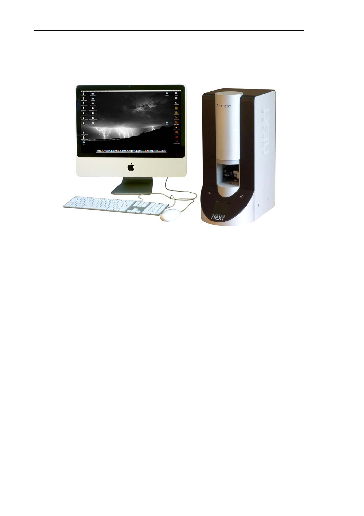
General view of the Solver NEXT SPM is shown in Fig. 1-1.
Fig. 1-1. General view of the Solver NEXT SPM
Solver NEXT SPM consists of the following main units:
● Solver NEXT measuring unit;
● SPM controller;
● Computer.
Besides, the delivery set of the Solver NEXT SPM can be optionally extended with:
● Measuring head for liquid environment;
● Liquid cell;
● Measuring head of the nanoindenter;
● Heating stage;
● Vibration isolation system.
Fig. 1-2 shows a schematic diagram of the Solver NEXT measuring unit.
6
Page 15
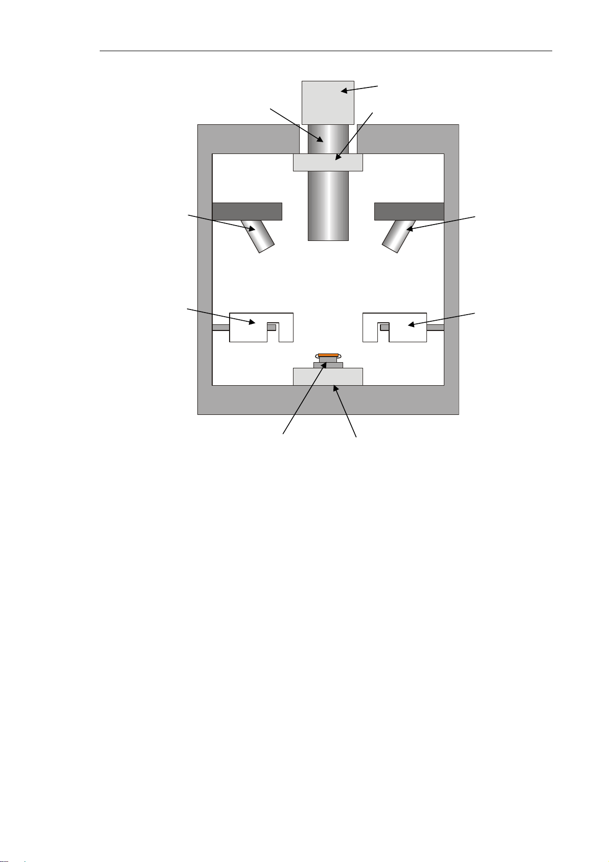
Video camera
Chapter 1. Overview
Optical microscope
Laser
STM measuring
head
Optical microscope
positioning system
Photodiode
AFM measuring
head
Sample
Fig. 1-2. Schematic diagram of the Solver NEXT
Sample positioning system
The sample to study is fixed on a metal substrate that is mounted on the sample holder. The
sample holder is fastened to the upper end of the piezo scanner that operates in the
“scanning-by-sample” mode.
The positioning system allows moving the sample in the XY plane to select the
investigation area as well as displacing the sample vertically to approach it to the probe.
The built-in optical viewing system serves for selecting the scan area on the sample
surface. The optical microscope of this system is equipped with a positioning system that
provides selection of the scan area on the sample surface.
The Solver NEXT measuring unit is equipped with two measuring heads, for atomic-force
microscopy (AFM) and for scanning tunneling microscopy (STM). Availability of two
built-in measuring heads enables quick exchange of the experimental technique and does
not need special training of the operator.
Auxiliary measuring heads (for liquid environment and for nanoindenting) extend range of
the instrument capabilities. With those heads, measurements in liquids as well as hardness
measurements or modification of the sample surface are available.
7
Page 16
Solver NE
X
P
i
b
o
a
n
e
g
n
n
o
r
n
g
o
M
F
v
n
.
e
a
h
t
e
t
e
bo
u
g
t
e
h
n
h
n
e
n
e
h
h
o
n
s
i
i
o
e
i
s
r
e
s
e
u
M
m
k
r
i
d
o
n
p
p
i
2
e
e
AFM
e
o
t
d
n
e
o
e
r
M
M
w
e
a
T SPM. Inst
uction Man
al
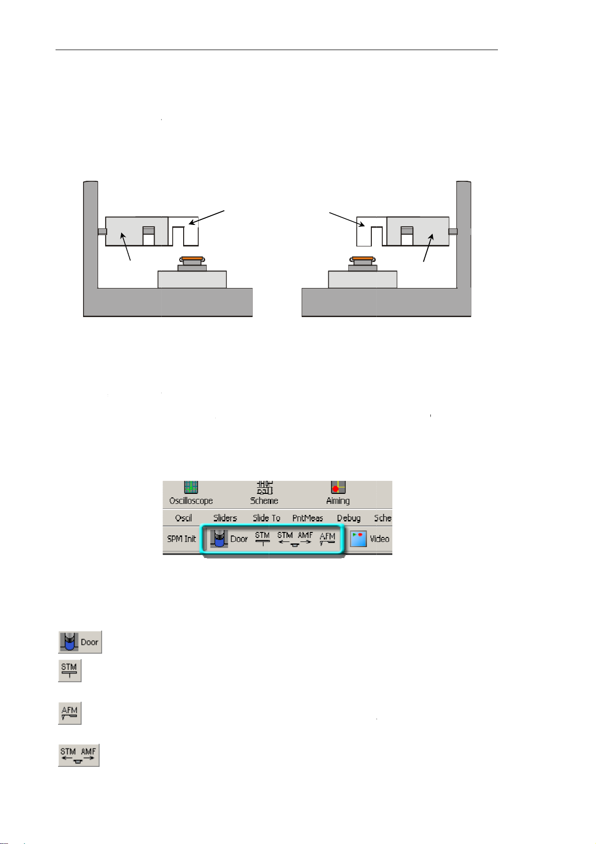
1.3.
The built-
asic stati
●
Inoper
●
Worki
ositio
n measurin
nary positi
tive positi
g position.
1
ST
ing the
heads are
ons (see Fi
n;
head
ig. 1-3. Sta
1 – inop
Built-i
located in
. 1-3):
2
ionary posit
rative posit
Meas
ide the SP
ons of the
on; 2 – wor
ring H
body. Th
easuring h
ing position
ads
y can stay
head
ads
in one of t
1
o
When a h
The worki
exchangin
Re-positio
control pa
Designati
ad is not in
ng positio
the probe
ing of th
el (see Fig
n of the he
– moves t
– moves
inoperativ
olved in t
is used i
With the
measuri
. 1-4) of th
Fig. 1-4
ds positio
e protectiv
he STM
position;
e current
the cours
ead being
g heads i
Control P
. Measurem
ing button
shield up
ead to its
peration, it
of measu
n this posit
controlle
ogram.
nt heads c
is followi
and down;
working
stays in its
ements as
on, the pr
through
ntrol panel
g:
osition an
inoperativ
well as in
be is abov
he Measu
the AF
position.
operations
the sampl
ement he
head to
on
.
ds
its
– moves
inoperativ
– moves
8
he AFM
position;
th heads t
ead to its
their inop
working
rative pos
osition a
tions.
d the ST
head to
its
Page 17

1.4. Technical Specification
Measuring system
Built-in measuring heads AFM, STM
Mountable measuring heads liquid, nanosclerometric
Chapter 1. Overview
System for detecting the cantilever
deflection
Laser wavelength of cantilever
deflection system
Sample
Size up to ø20×10 mm
Positioning range, in XY plane 5×5 mm
Positioning method automated with the use of optical image
Minimum positioning step
Sample weight up to 40 g
Heating capabilities
(heating stage)
Scanning system
Scanning mode by sample
Scan area
automated alignment
850 nm
0.3 μm
up to 150 °C
100×100×10 μm (±10 %)
3×3×2.6 μm (±10 %)
(in the high resolution mode)
Relative error of distance
measurement:
XY plane
Z direction
Non-linearity, in XY plane (with the
use of feedback sensors)
RMS noise in 1 ÷ 200 Hz frequency
range, XY plane
RMS noise in 10 ÷ 1000 Hz frequency
range, Z direction:
with the use of the feedback sensors
in the high resolution mode
less 1 % (less 0.1 % with the use of the feedback
sensors)
less 5 %
less 0.1 %
less 0.02 nm (XY 100 μm)
less 0.001 nm (XY 3 μm)
less 0.04 nm
less 0.02 nm
9
Page 18

Solver NEXT SPM. Instruction Manual
Optical viewing system
Positioning range, 5×5 mm
Positioning step
Resolution
Field of view
0.3 μm
2 μm
3.4 ÷ 0.53 μm
Dimensions and weight
Overall dimensions
320×215×470 mm
Weight 30 kg
Power characteristic
Voltage 110/220 V
Power consumption less 400 W
10
Page 19

Chapter 2. Basic Safety Measures
2. Basic Safety Measures
General Safety Measures
● Ground the instrument before operation!
● Do not disassemble any part of the device. Disassembling of the product is permitted
only to persons certified by NT-MDT.
● Do not connect additional devices to the instrument without prior advice from an
authorized person from NT-MDT.
● This instrument contains precision electro-mechanical parts. Therefore protect it from
mechanical shocks.
● Protect the instrument against the influence of extreme temperature, the direct impact
of sun radiation, and moisture.
● For transport, provide proper packaging for the instrument so as to avoid its damage.
Electronics
● To reduce possible influence of power line disturbances on the measurements, we
recommend supplying the instrument units with a surge filter.
● Before operation, set the power switch of the SPM controller to the position
corresponding to value of the local electrical power line (this is only done with the
controller being off!).
● Switch the SPM controller off before connecting/disconnecting its cable connectors.
Disconnecting or connecting the cable connectors during operations may cause damage
to the electronic circuit and disable the instrument. A warning label is attached to the
SPM controller of the instrument (Fig. 2-1).
Fig. 2-1
11
Page 20

Solver NEXT SPM. Instruction Manual
Laser
● Observe safety measures for operation with devices containing sources of laser
radiation. Do not stare into the beam. A label warning about the presence of laser
radiation is attached to the rearing panel of the measuring unit.
Fig. 2-2
Scanner
● Do not apply to the scanner forces bigger than it is necessary for installation of a probe
or a substrate with a sample. Avoid impacts on the scanner and its lateral displacement.
Remember that thickness of the scanner walls makes only 0.5 mm.
12
Page 21

Chapter 3. Operating Conditions
3. Operating Conditions
The SPM should be installed in a room of total area larger 6 sq. meters with range of purity
better 8 (by ISO 14644-1-2002).
To provide for the qualitative and safe operation of the instrument, it is recommended to
observe the following conditions:
● environment temperature:
● ultimate range (15–35) °С;
● recommended range (20–25) °С.
● temperature drift: less 1˚C per hour;
● relative humidity:
● ultimate range (20–80) % (moisture condensation prevented);
● recommended range (30–50) % (moisture condensation prevented).
● vibration amplitude
in the band 1 ÷ 1000 Hz less 0.5 µm;
● atmospheric pressure (760±25) mm Hg/(100±4) kPa;
● the work area should be supplied with a protective grounding circuitry and with
grounded electric mains (110/220 V);
● electric mains:
● voltage (110±10)/(220±22) V;
● frequency (50.0±0.4)/(60±0.5) Hz;
● the room should be protected from mechanical vibrations and acoustic noises, either
internal or external;
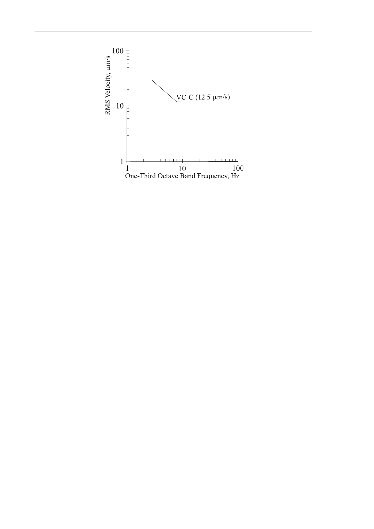
● vibration criterion VC-C, 12.5 µm/s (one-third octave band criterion);
13
Page 22
Solver NEXT SPM. Instruction Manual
● the table intended for installation of the instrument measuring unit must be stable and,
whenever possible, massive;
● to provide solid stability against vibrations, SPM modules should be placed on self-
leveling floor with marble covering alongside bearing components of the building
(pillows, beams etc.);
● the measuring unit of the instrument (the approach unit with the measuring head)
should be placed on a separate table away from computers and monitors, to eliminate
electromagnetic interference;
● the instrument should be protected from the direct impact of sun radiation;
● the operation of the device is susceptible to heat flows, draughts and sudden
alternations in temperature and humidity.
14
Page 23

Chapter 4. Regulations on Packaging, Storage and Transportation
4. Regulations on Packaging, Storage and
Transportation
● Packaging of the equipment should be performed indoors in a ventilated room at
ambient temperature of 15° С – 40 °С and relative humidity at most 80 % with no
corrosive agent in the atmosphere. Storage conditions should comply with the standard
GOST 15150.
● The equipment should be carried by one or several modes of enclosed transport
according to transport regulations applicable to the mode(s) in service.
● Only transportation of the equipment in proper package is permitted to prevent
transportation damage.
● The equipment in its package should be placed and secured in a vehicle in a way that
provides steady position and excludes shocks of the deliverable parts by one another or
by walls of the vehicle.
● Transportation conditions should comply with requirements of the standards
GOST Р 52931-2008 and GOST 15150.
● Transportation and storage in regions of the Far North and equated localities should
comply with requirements of the standards GOST Р 52931-2008 and GOST 15846.
● Location of the equipment in a warehouse must provide easy access to it and free space
for personnel.
● Devices and their parts should be stored on shelves.
● At least 100 mm distance between the stored parts and walls and ceiling of the
premises should be reserved.
● Distance between the stored parts and heating facilities of the premises should be at
least 0.5 m.
15
Page 24
Solver NEXT SPM. Instruction Manual
5. Setup and Installation
5.1. Connecting the Electromechanical Units
ATTENTION! Before connecting or disconnecting any unit, switch off
the controllers. Disconnecting or connecting cables while the devices are
operating may cause damage to their electronic circuits.
1. Place the computer on its stationary location.
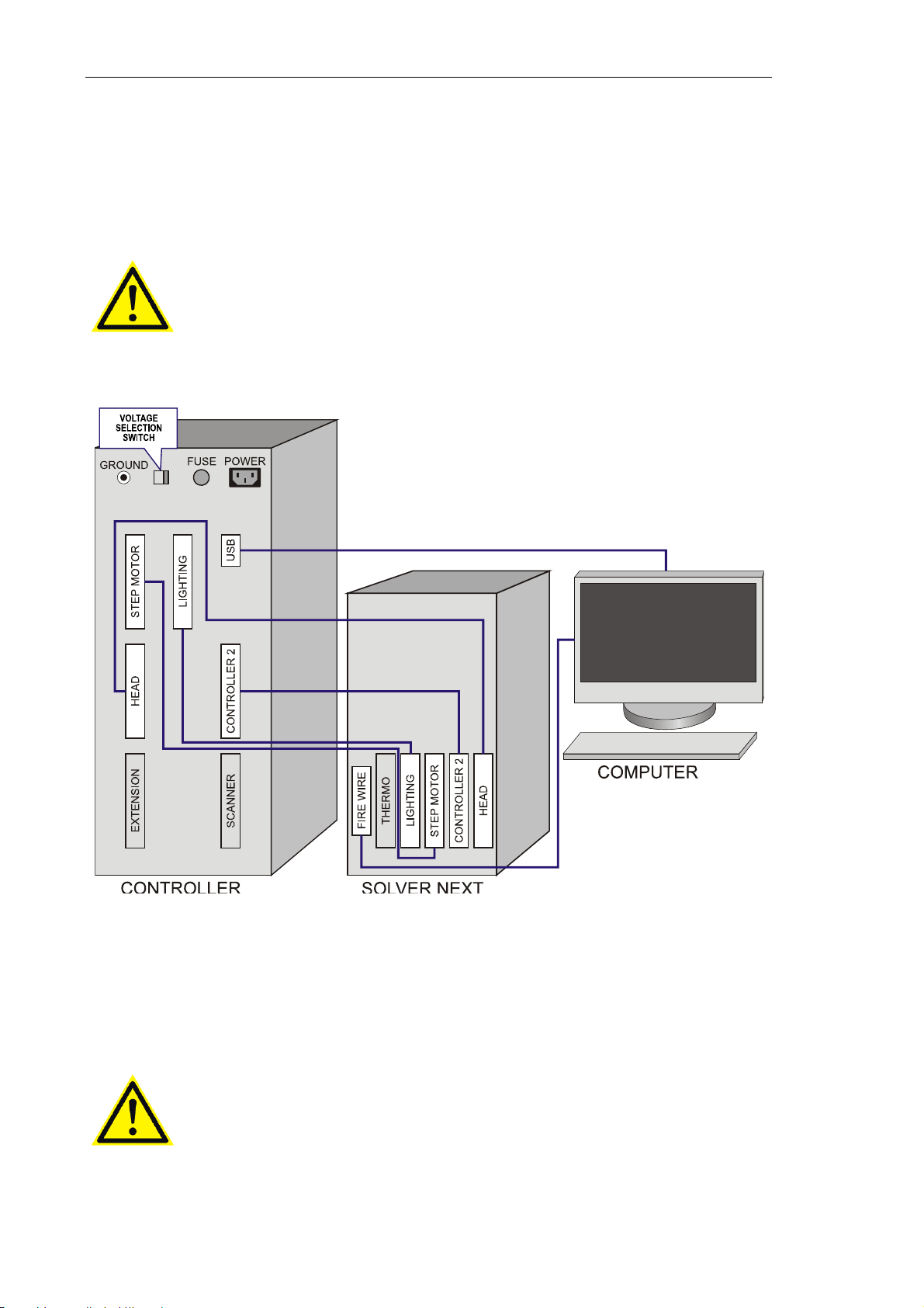
2. Perform cable connections according to the diagram of Fig. 5-1.
Fig. 5-1. Cable connections
3. Turn the voltage switch of the SPM controller to the position corresponding to the
actual voltage of the mains supply. The controller must be off at the moment of
switching!
4. Connect the SPM controller to the mains supply.
ATTENTION! The SPM controller can be connected to an electrical
power supply line of 110/220 V (60-50 Hz) after setting the voltage
selection switch to the position corresponding to this power supply line.
Observe this instruction to prevent damage of the electronic
components.
16
Page 25
Chapter 5. Setup and Installation
5.2. Installing Software
Nova P9 program doesn't need special installation procedure. Just insert the software CDROM in the computer CD-drive and copy the content of Nova P9 folder to the desired
location of your hard drive. With the program installed, install drivers of the scanning
probe microscope controller.
To install the controller's drivers, perform the following steps:
1. Connect the SPM controller to the computer. This will make the operating system to
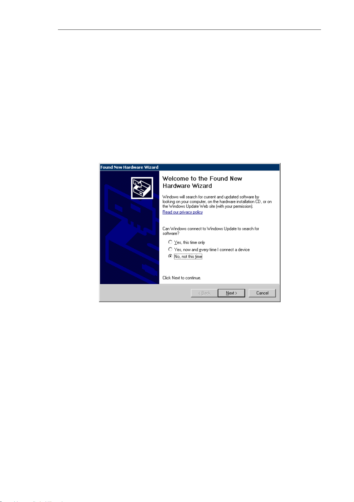
detect a new hardware USB <-> Serial and to open the Found New Hardware Wizard
dialog.
Fig. 5-2.
Found New Hardware Wizard window
To install the software driver for the USB <-> Serial hardware, perform the following
steps:
a) Skip the Windows Update option in the Found New Hardware Wizard dialog by
selecting the No, not this time option and click the Next button.
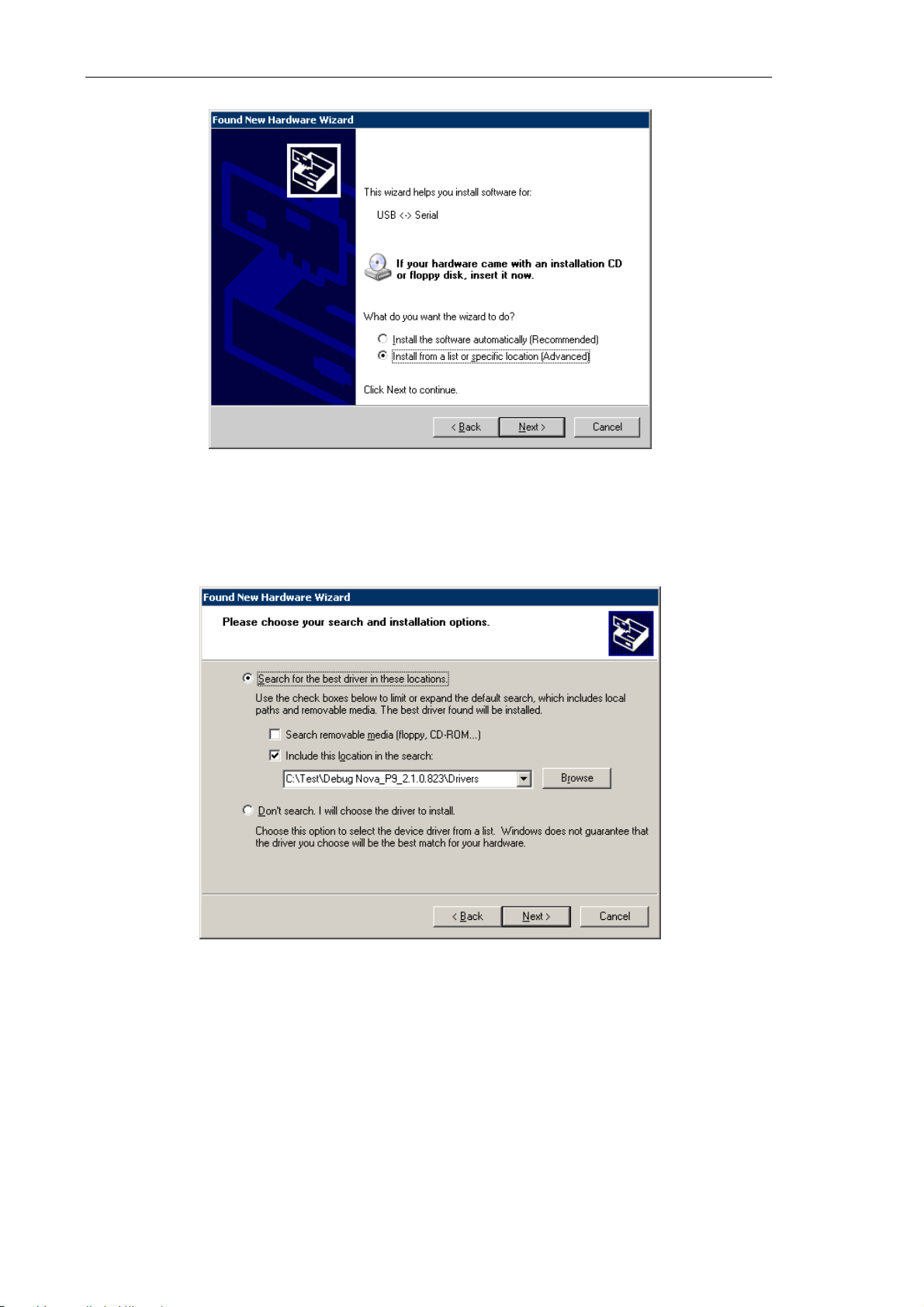
b) The installation wizard will ask how to find location of drivers on your computer.
Select the Install from a list or specific location option that allows for manual
defining the path of drivers location. Click the Next button.
17
Page 26
Solver NEXT SPM. Instruction Manual
Fig. 5-3
c) For defining the desired path, select the options Search for the best driver in these
location and Include this location in the search and then click the Browse button.
Fig. 5-4
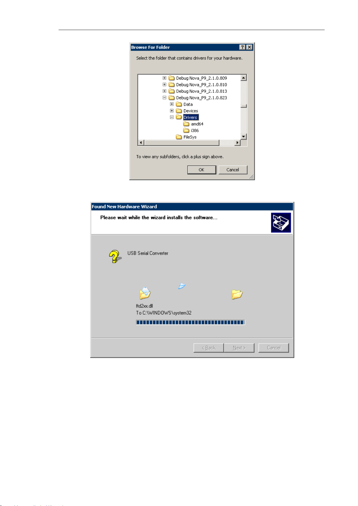
d) The Browse For Folder dialog will open. Select the Drivers subfolder in the Nova
P9 program folder and click the ОК button. This will start installing the controller's
driver.
18
Page 27
Chapter 5. Setup and Installation
Fig. 5-5.
Browse For Folder window
Fig. 5-6. Installing the controller's driver
e) When installing the drivers of the USB <-> Serial hardware completes, click the
Finish button. The installation wizard will close.
19
Page 28
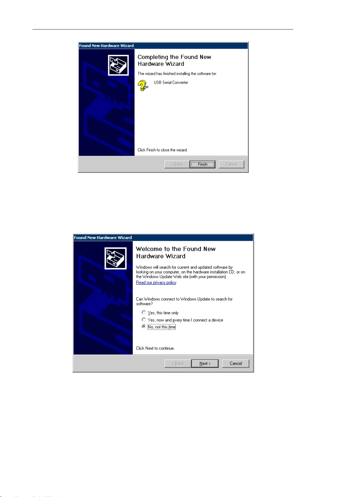
Solver NEXT SPM. Instruction Manual
Fig. 5-7
2. With the drivers of the USB <-> Serial hardware installed, the operating system will
find another hardware, USB Serial Port, and open the Found New Hardware Wizard
dialog again.
Fig. 5-8.
Found New Hardware Wizard window
To install the software driver of the USB Serial Port hardware, perform the following
steps:
a) Skip the Windows Update option in the Found New Hardware Wizard dialog by
selecting the No, not this time option and click the Next button.
20
Page 29
Chapter 5. Setup and Installation
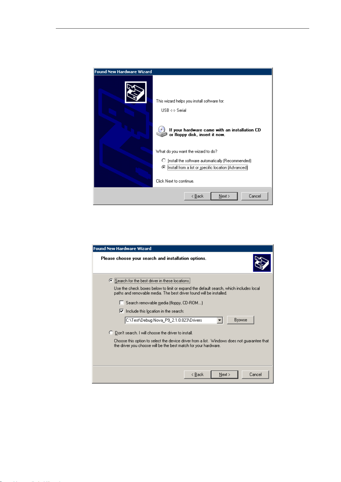
b) The installation wizard will ask how to find location of drivers on your computer.
Select the Install from a list or specific location option that allows for manual
defining the path of drivers location. Click the Next button.
Fig. 5-9
c) For defining the desired path, select the options Search for the best driver in these
location and Include this location in the search and then click the Browse button.
Fig. 5-10
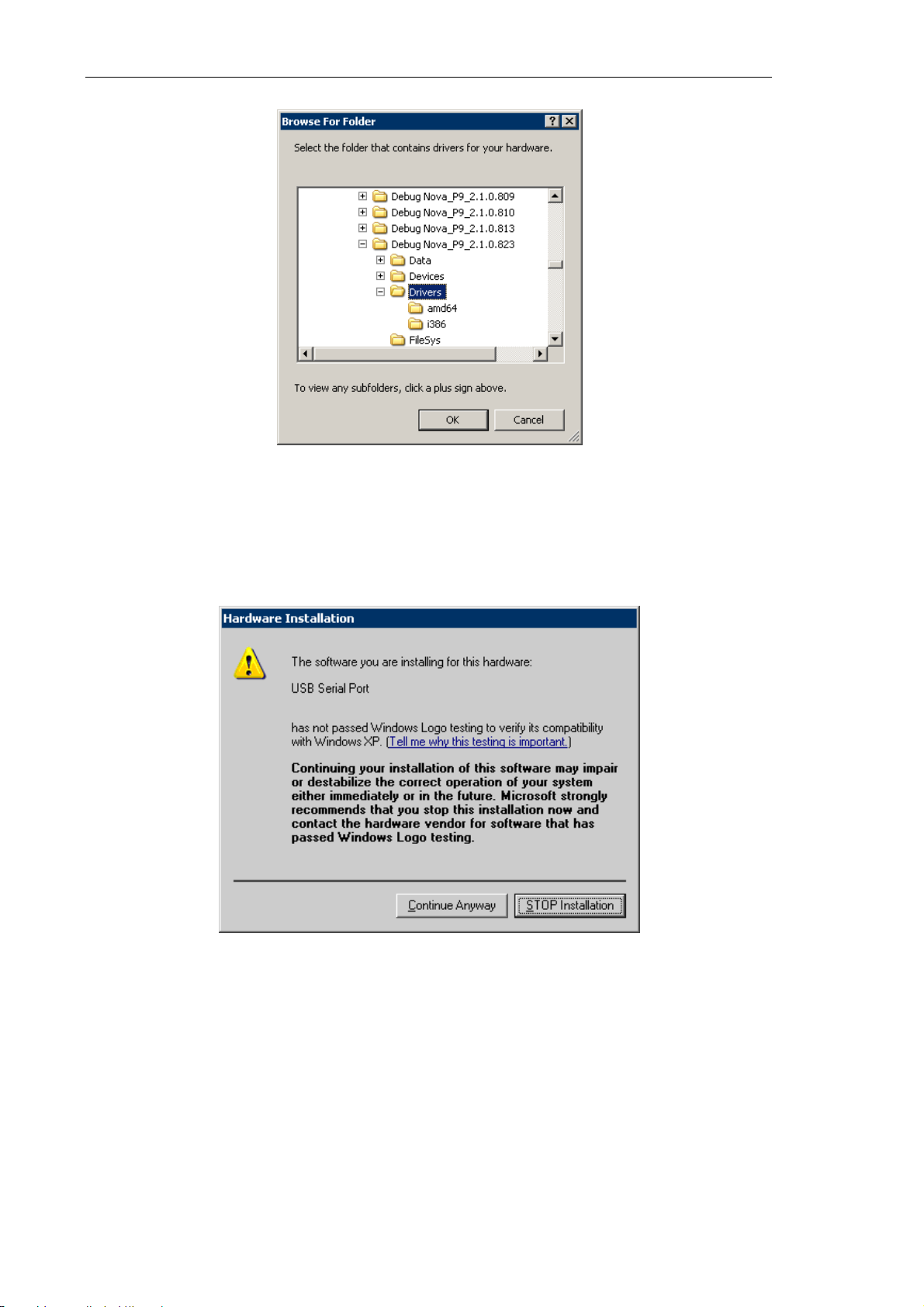
d) The Browse For Folder dialog will open. Select the Drivers subfolder in the Nova
P9 program folder and click the ОК button. This will start installing the controller's
driver.
21
Page 30
Solver NEXT SPM. Instruction Manual
Fig. 5-11.
Browse For Folder window
e) The Hardware Installation window will open to inform that the tested hardware is
incompatible with the operating system. Click the Continue Anyway button. This
will start installing the driver of the controller's USB port.
22
Fig. 5-12.
Hardware Installation window
Page 31
Chapter 5. Setup and Installation
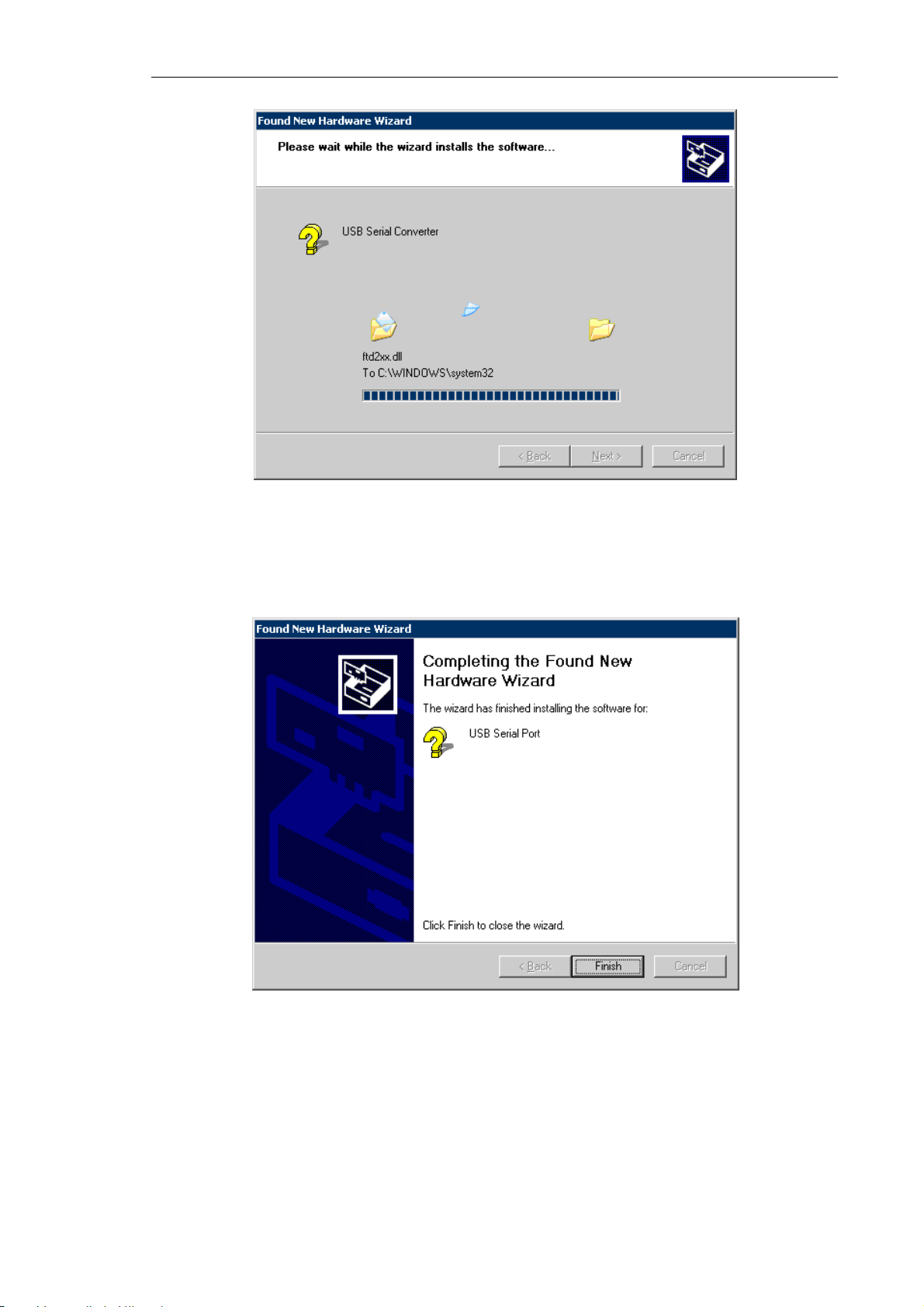
Fig. 5-13. Instaiing the driver of the controller's USB port
f) When installing the drivers of the USB Serial Port hardware completes, click the
Finish button. The installation wizard will close.
Fig. 5-14
23
Page 32
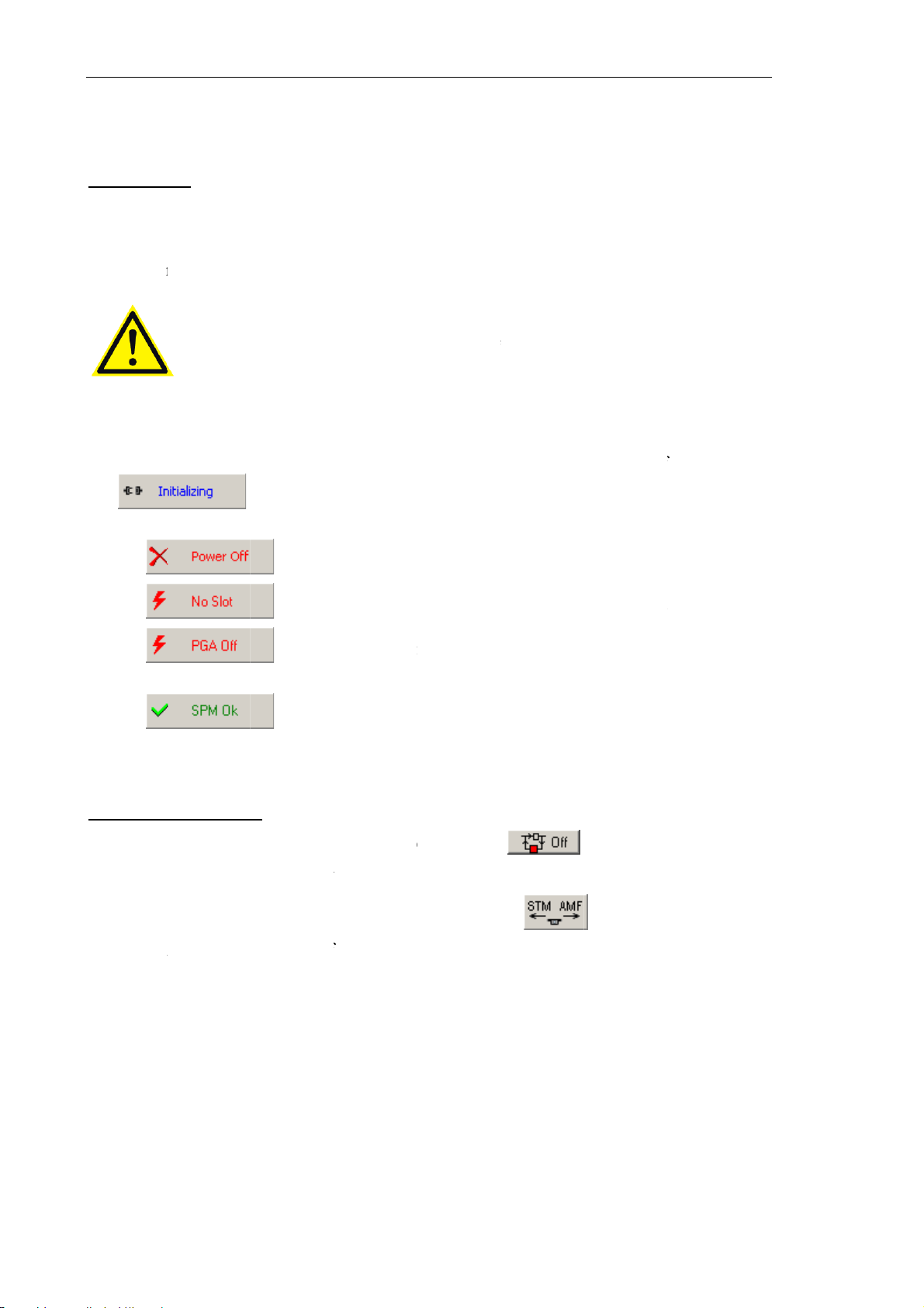
Solver NE
X
P
h
h
n
h
t
n
e
t
t
h
h
t
r
r
n
c
N
m
ge
a
c
o
a
a
o
n
p
u
i
c
o
t
n
h
l
i
P
h
h
t
e
f
r
o
m
r
n
b
o
n
p
t
.
b
e
M
e
n
t
f
h
d
n
w
m
n
f
t
t
)
e
o
o
f
o
a
e
t
u
n
t
o
T SPM. Inst
uction Man
al
5.3.
Switching
1. Turn t
2. Turn t
3. Turn o
4. Start t
5. The p
states:
●
owerin
on
e compute
e vibratio
the SPM
ATTE
instru
dama
e Nova P9
ogram st
g Sequ
on.
protection
ontroller.
TION! Al
ent on. D
to the ele
Control Pr
rts with
indicator i
– t
ence
system on.
l connecto
sconnecti
tronic co
gram. The
he testing
the
Initia
e controlle
s should
n of conn
ponents.
Program
procedur
lization
is off;
e tightene
ctors duri
ain windo
. On co
pa
el takes o
up befor
operati
appears
pletion o
e of the f
turning
n may ca
n the scree
testing,
llowing f
he
se
.
he
ur
●
●
ini
●
Completi
1. Disabl
2. Retrac
3. Move
4. Switc
5. Turn t
6. Close
ialization,
operati
the feedb
the probe
he heads t
the SPM c
e vibratio
he control
– s
–
lick the
S
– t
n
ck loop (t
way from
their inop
ontroller o
protection
rogram.
ots address
nitializatio
M Init
utt
e instrume
e button a
he sample.
rative posi
f.
system off
es in the In
of the
n on the
t is ready
pearance is
ions with t
erface.ini
instrumen
In
itialization
or operatio
e
ile are inv
is need
oolbar.
n.
.
button.
lid;
. To st
rt
24
Page 33
Chapter 5. Setup and Installation
5.4. Calibrating the Stepper Motors
Stepper motors of the instrument should be calibrated after installation of equipment and/or
control software as well as after repairing malfunction of the instrument (e.g., caused by
power failure).
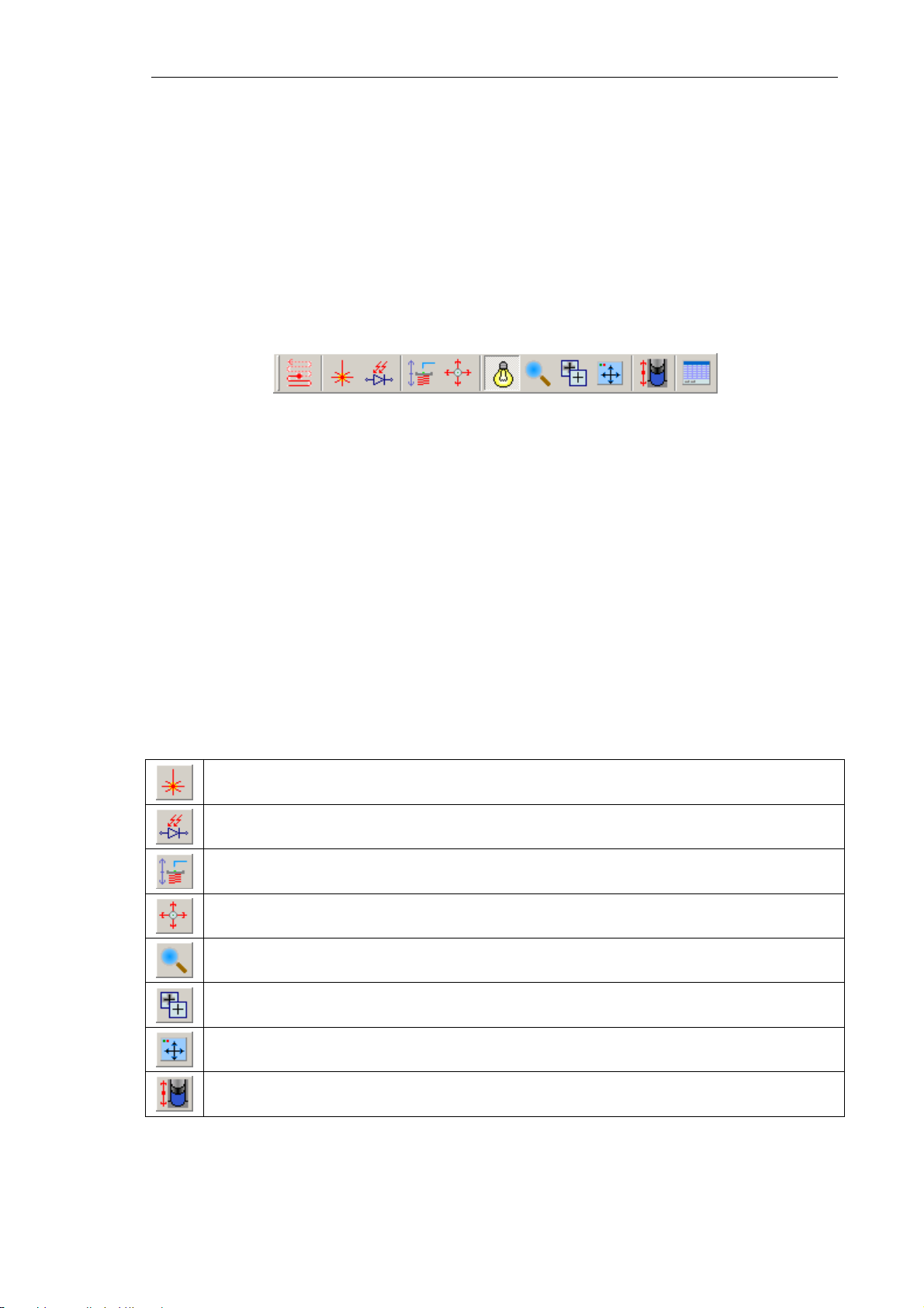
The Next Motors panel provides controls of all instrument modules that contain stepper
motors. Calibration of the stepper motors is required for correct operation of the
instrument.
Fig. 5-15.
Next Motors panel
To calibrate the stepper motors, perform the following steps using the Next Motors panel:
1. Open the stepper motors control window of the desired module by clicking the
corresponding button (see Table 1 below).
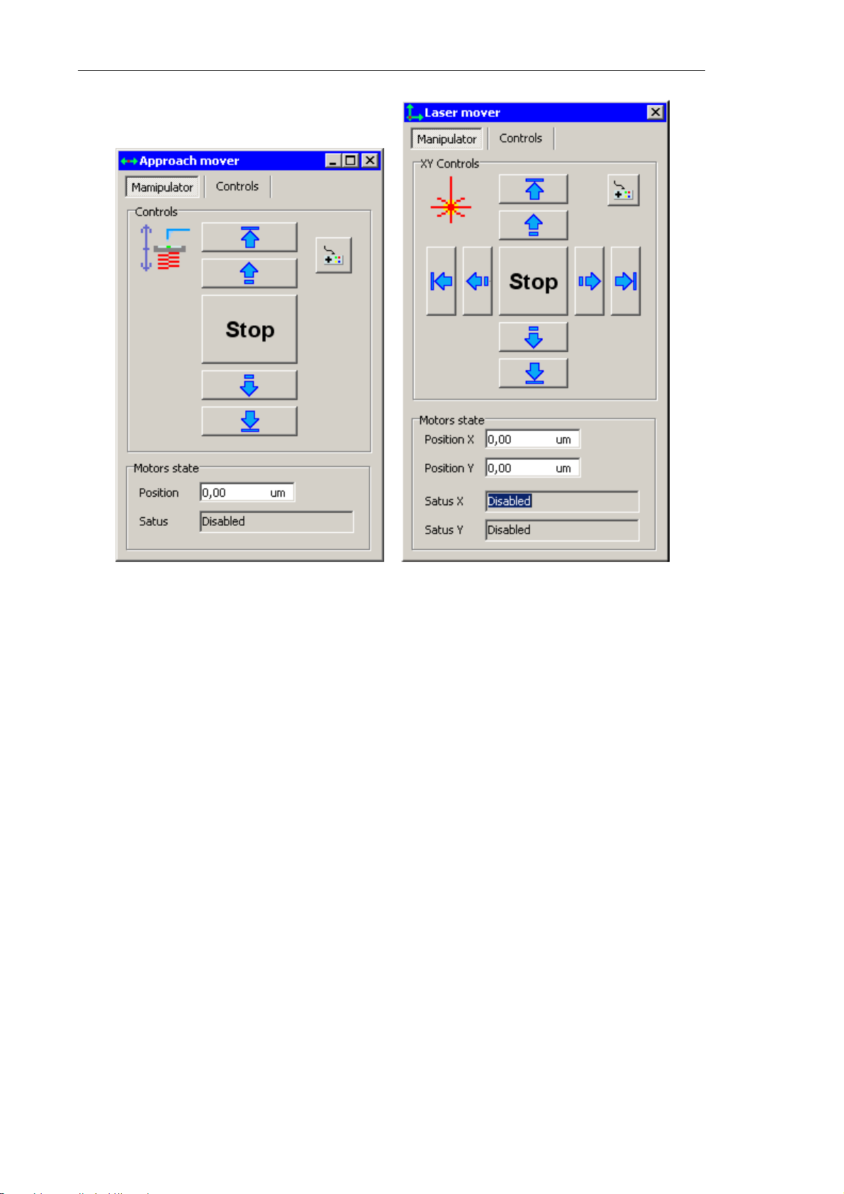
NOTE. The instrument modules employ one or two stepper motors. Appearance of the
stepper motors control window is that shown in Fig. 5-16 a for modules with one motor
or shown in Fig. 5-16 b for modules with two motors.
Table 1. Buttons for opening stepper motors control windows
of specific modules
Laser stepper motors.
Photodiode stepper motors.
Stepper motor of sample vertical displacement.
Stepper motors of sample lateral displacement.
Stepper motor of videomicroscope vertical displacement.
Stepper motor of videomicroscope focus.
Stepper motors of videomicroscope lateral displacement.
Stepper motor of the protective shield.
25
Page 34
Solver NEXT SPM. Instruction Manual
a) Control window for one motor b) Control window for two motors
Fig. 5-16. Stepper motors control window
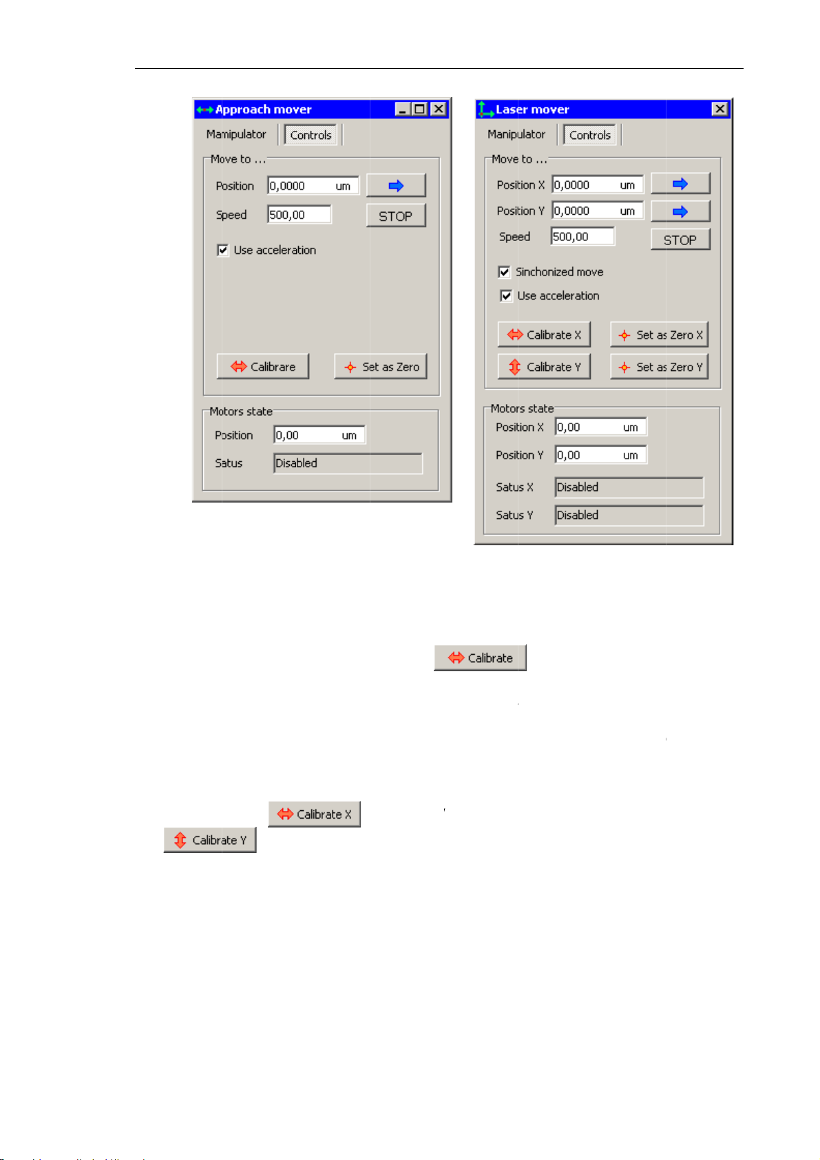
2. Switch to the Controls tab (Fig. 5-17).
26
Page 35
i
k
l
d
r
If
s
i
(
w
i
o
e
n
1
n
m
t
g
e
b
h
p
l
.
c
d
o
d
d
a
a
i
s
e
m
i
Chapter
d
a
T
r
c
f
t
t
e
o
d
m
i
u
c
X
e
n
n
7
r
,
o
e
s
t
(
e
5. Setup an
Installatio
3.
Start the
motor w
then bac
its initia
redefine
of the cu
NOTE.
motor (u
a) Control
calibration
ll move th
ward until
position.
according
ent positi
a module
e the
butto
indow for o
F
g. 5-17. Ste
procedure
e driving
the opposi
Total ran
to the dete
n will be r
mploys tw
).
e motor
pper motors
with the
icroscrew
e limit sto
e of avai
cted range
calculated
o motors,
utton) an
control win
of the mo
, and, fin
able displ
of motor d
alibration
then proc
b)
Control win
ows. Calibr
button.
ule forwa
lly, the mi
cement o
splacemen
hould star
ed with th
ow for two
tion tab
he gear of
d until the
roscrew w
the mod
. As well,
with the
Y movem
otors
the steppe
limit stop
ll return t
le will b
oordinate
movemen
nt motor
4.
Complet
window
on of the
see Fig. 5-
calibration
8). Click t
procedure
e OK butt
is confir
n in this w
ed by a c
ndow.
rrespondi
g messag
2
Page 36
Solver NE
X
r
u
o
d
m
T SPM. Inst
uction Man
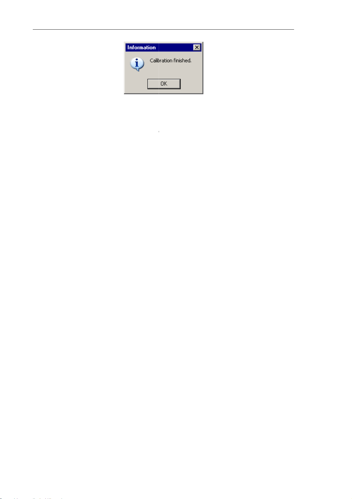
al
5. Apply
calibration
to all stepp
Fig. 5-18. M
er motors
essage win
f the instru
ow
ent.
28
Page 37
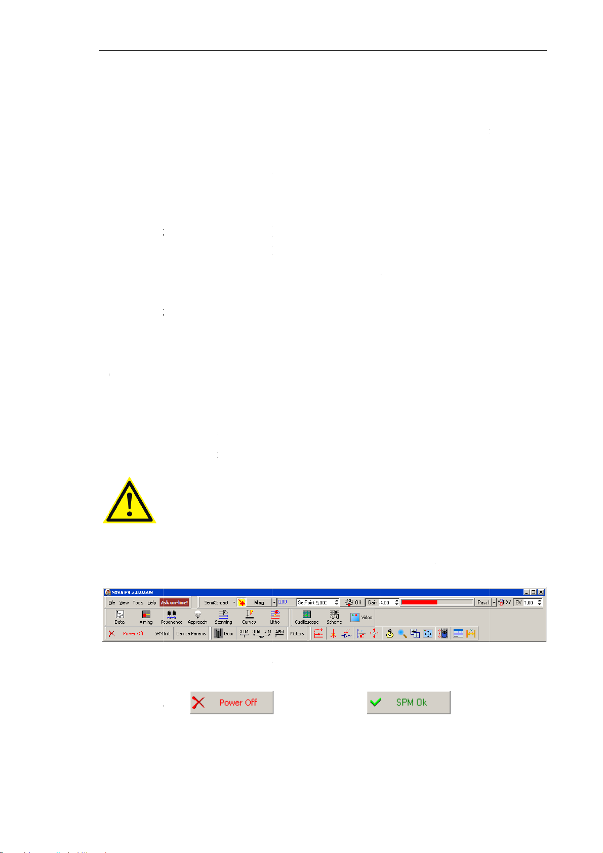
6
hse
6
o
h
p
t
O
g
g
g
g
g
p
g
u
n
t
t
r
o
e
h
d
t
l
(
r
P
e
e
A
O
o
o
n
T
n
w
e
e
t
d
2
.
(
h
c
o
c
u
h
c
r
N
)
a
z
m
d
o
5
t
.
n
r
p
h
f
h b
a
Ch
a
r
s
p
m
o
o
m
n
p
M
6
a
u
d
n
e
m
t
p
n
s
9
e
e
e
e
,
pter 6. Pre
aring for M
asurement
. Pre
T
is chapter
quence of
1.
Turning
2.
Mountin
3.
Installin
4.
Selectin
5.
Screenin
Adjustin
6.
7.
Initial A
8.
Selectin
.1. T
aring
explains t
hose proce
n (see sec
the Samp
the Probe
the Measu
with the
the Cantil
proach (se
the Scan
rning
for M
e prepara
ures inclu
. 6.1 on p.
e (see sect.
see sect. 6
ing Head
rotective S
ver Defle
sect. 6.8
rea (see se
n Instr
asure
ory proce
es the foll
9).
6.2 on p. 3
4 on p. 34)
see sect. 6.
ield (see s
tion Detec
n p. 51).
t. 6.9 on p
ment
ents
ures requi
wing step
).
.
on p. 40).
ect. 6.6 on
ion Syste
52).
ed for AF
:
. 41).
(see sect.
measure
.7 on p. 41
ents. Th
).
T
turn the i
1.
Turn the
2.
Turn on
3.
Start up
compute
The prog
strument
computer
he SPM co
ATTEN
instrume
damage t
he control
monitor (s
ram starts
n, perform
n.
troller wit
ION! All
t on. Disc
o the elect
program
ee Fig. 6-1
Fig. 6-1. M
ith initiali
the followi
the powe
onnectors
onnection
onic com
ova P9. T
.
in window o
ation of t
g steps:
switch on
should be
of connect
onents.
e main pr
the progra
e instrume
the front p
tightened
rs during
gram win
Nova P9
t. As the i
nel.
p before
operation
ow will ap
itializatio
urning th
may caus
ear on th
completes
caption
T
e instrum
f the
nt is now r
ady for op
utton ch
eration.
nges to
.
2
Page 38
Solver NE
X
M
m
s
t
e
e
e
e
r
m
a
e
a
n
u
g
u
s
t
h
a
t
p
t
s
r
a
s
g
s
p
F
e
b
b
m
p
t
o
w
e
k
e
h
n
e
d
t
m
n
i
t
p
T SPM. Inst
uction Man
al
6.2.
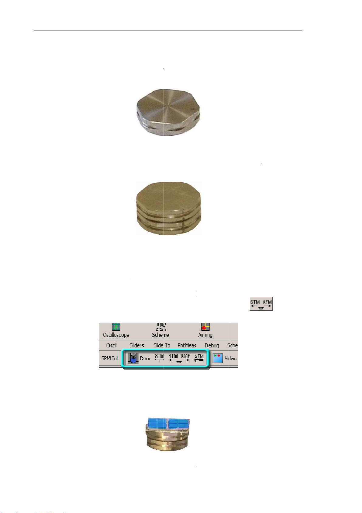
A sample
the instru
If thickne
(see Fig. 6
ountin
to study is
ent.
s of the sa
-3).
g the S
mounted o
Fig
ple is les
ample
n a standa
. 6-2. Stand
3 mm, it s
d metal su
rd metal su
hould be
strate (see
strate
ounted on
Fig. 6-2)
a stack of
elivered w
wo substra
th
es
To mount
1. If any
install
the M
2. Fix th
thickn
he sample,
of the me
d/exchang
asuring he
sample o
ss) with gl
Fig. 6-3. S
perform t
suring he
d, retract i
ds control
Fig. 6-4
a substra
e or doubl
ack of two
e followin
ds is at it
to the ino
anel (see
. Measurem
e or on a
e-sided stic
ubstrates fo
steps:
working
erative sta
ig. 6-4).
nt heads c
stack of t
ky tape (se
r thin sampl
osition w
e by clicki
ntrol panel
o substrat
Fig. 6-5).
s
en the sa
g the
s (regardi
ple is to
button
g the sam
be
in
le
Fi
. 6-5. Thin
30
ample fixed
to the stac
of two subs
trates
Page 39
Chapter 6. Preparing for Measurements
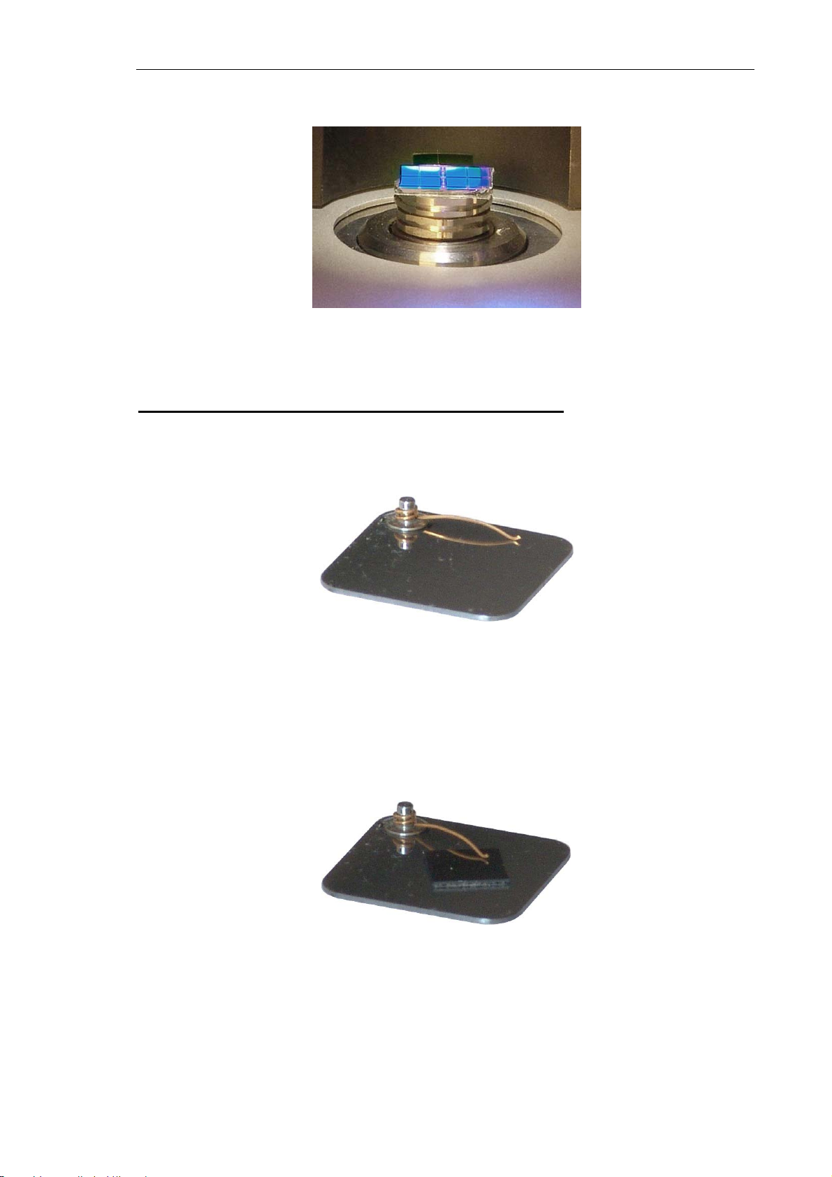
3. Place the sample-substrate assembly on the scanner magnetic fastener (see Fig. 6-6).
Fig. 6-6. Sample-substrate assembly placed on the scanner magnetic fastener
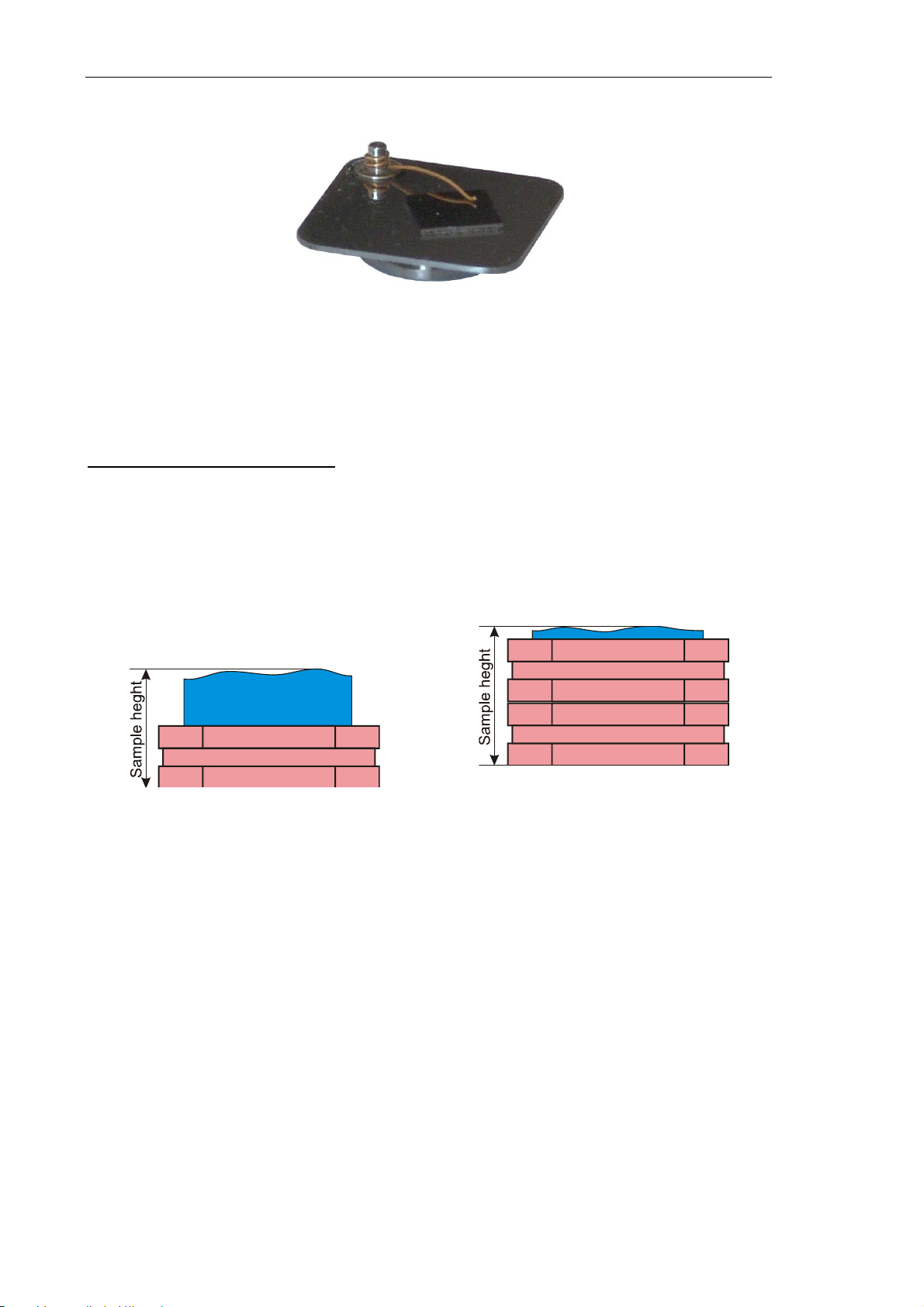
Mounting the sample on a substrate with the spring contact
For measurements requiring electrical contact between the sample and the instrument, it is
recommended to use a specialized substrate equipped with the spring contact
(see Fig. 6-7).
Fig. 6-7. Substrate with the spring contact
1. Fix the sample on the substrate with the spring contact with glue or double-sided sticky
tape.
2. Move the spring contact with tweezers and place it close to the edge of the sample
(see Fig. 6-8).
Fig. 6-8. Sample mounted on the substrate with the spring contact
31
Page 40
Solver NEXT SPM. Instruction Manual
3. Place the sample-substrate assembly on a standard metal substrate (see Fig. 6-9).
Fig. 6-9. Sample-substrate assembly placed
on a standard metal substrate
4. Place the assembly of the sample and the two substrates on the scanner magnetic
fastener.
Setting the sample height value
Height of the sample above the scanner surface is important for accuracy of scan results.
For the sample height, the Control program Nova P9 reserves the Sample Height
parameter.
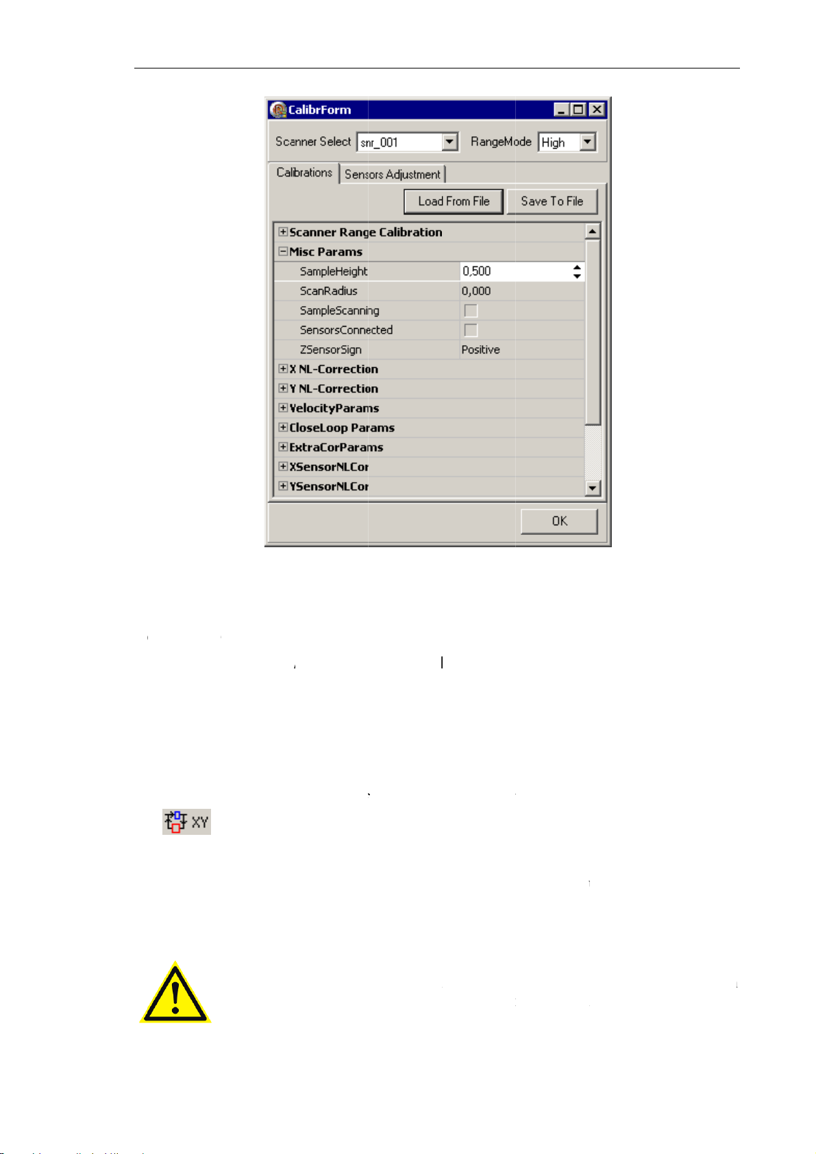
Take height of the sample-substrate(s) assembly (see Fig. 6-10) and assign this value to the
SampleHeight parameter of the Control program.
a) Assembly of a thick sample and a substrate
Fig. 6-10. Definition of the
SampleHeight parameter
b) Assembly of a thin sample and two
substrates
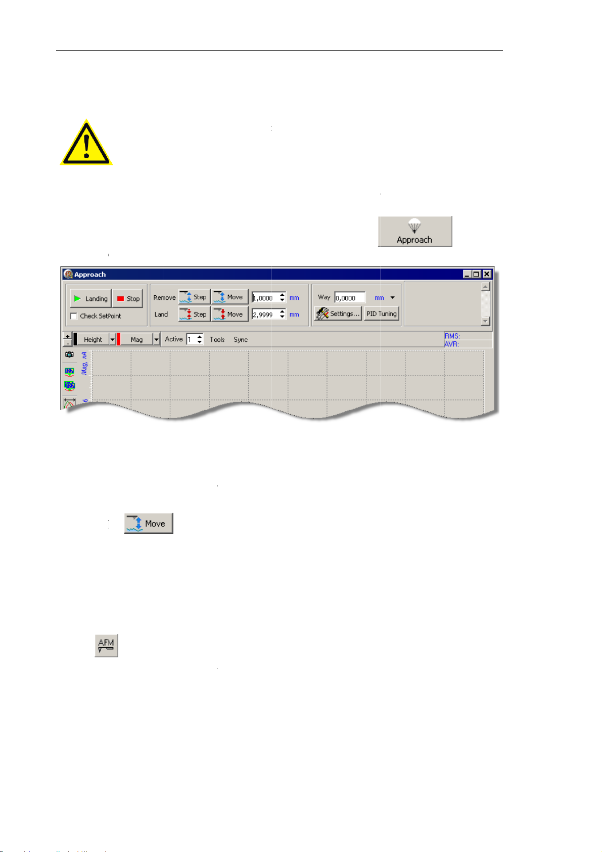
To define the sample height, enter the measured value of the sample height (in mm) in the
SampleHeight field of the Misc Params parameter group of the CalibrForm dialolg
(Fig. 6-11) (accessible through the
Tools Æ Calibration menu command).
If the sample height changes, redefine the SampleHeight parameter of the CalibrForm
dialog.
32
Page 41
6
h
hTolo
e(SC
C
l
b
t
-
t
e
m
CA
s
C
e
s
o
T
e
e
™
v
)
m
f
p
o
a
n
m
u
s
a
n
t
nnging
Ch
a
s
o
o
b
o
g
o
m
p
o
w
.
O
u
(
c
h
e
S
n
w
c
L
1
a
s
3
r
e
g
n
e
m
pter 6. Pre
aring for M
asurement
.3. S
T
e SCANS
●
"high vo
XY feed
●
"low vol
signal-to
●
T
e low-vol
select th
w-voltage
lecting
ANS
ALER™
tage" – the
ack loop (
age" – th
noise ratio
i
s released).
age mode i
desired m
ode) in th
Fig. 6-11
Op
LER
ystem pro
maximum
lose Loop
maximu
, the XY
usually a
de, select
e
Range M
. Calibratio
rating
Syste
ides meas
scan area i
;
scan are
eedback lo
plied whe
either
de
High
list of
parameter
M
)
rement in
at least 10
is approx
op should
high, up t
(for the hi
he
CalibrF
dialog
de
ne of the t
0×100 m
imately 2×
e open (
size, resol
h-voltage
rm
dialog
f
o followi
Scanning
2 m. For
pen Loop,
tion is ne
mode) or
see Fig. 6-
canne
g modes:
ill use th
improvin
the butto
essary.
ow
(for th
1).
ATTEN
the prob
ION! Avoi
before ch
d damagi
the
the prob
operating
e by retra
ode of t
ting the s
e scanner.
mple fro
3
Page 42
Solver NE
X
n
h
s
t
e
a
App
h
o
h
r
g
N
t
p
A
c
m
h
d
n
h
m
n
n
u
r
B
r
o
a
F
÷
o
F
o
h
u
y
t
e
h
6
Ap
b
m
l
h
r
m
v
h
w
p
n
h
w
l
o
e
t
n
p
t
i
T SPM. Inst
uction Man
al
6.4. I
To place t
following
1. Open
the
Op
stallin
ATTE
magne
not to
e scanner
teps:
he
pproa
ration For
the P
TION!
ic fastene
revent m
magnetic f
h
window
s
toolbar
obe
efore ins
should b
vement of
stener wit
(see Fig.
of the Cont
alling/exc
placed at
the measu
the sampl
-12) by cli
rol Progra
anging t
its lowest
ing head.
e at its lo
cking the
.
e probe,
extreme f
est extrem
the scan
r the sam
, perform
button
er
le
he
in
2. Type
the
3. Click t
6.4.1.
To install
1. Move
the
2. Turn t
value in t
roach
win
e
Installi
r replace t
the AFM
button i
e measuri
e range 10
ow.
button t
g the A
e AFM pr
easuring
the Meas
g head to
ig. 6-12.
15 mm in
move the
M Pro
be, perfor
ead to its
ring heads
ou manual
proach
the
sample to t
win
Remo
e
the follo
working
control pa
y (see Fig.
ow
e
input fie
e extreme
ing steps:
osition (se
el (see Fig.
6-14).
in the co
lower posi
e Fig. 6-13
6-4).
ntrol panel
ion.
) by click
of
ng
34
Page 43
Chapter 6. Preparing for Measurements
Fig. 6-13 Fig. 6-14
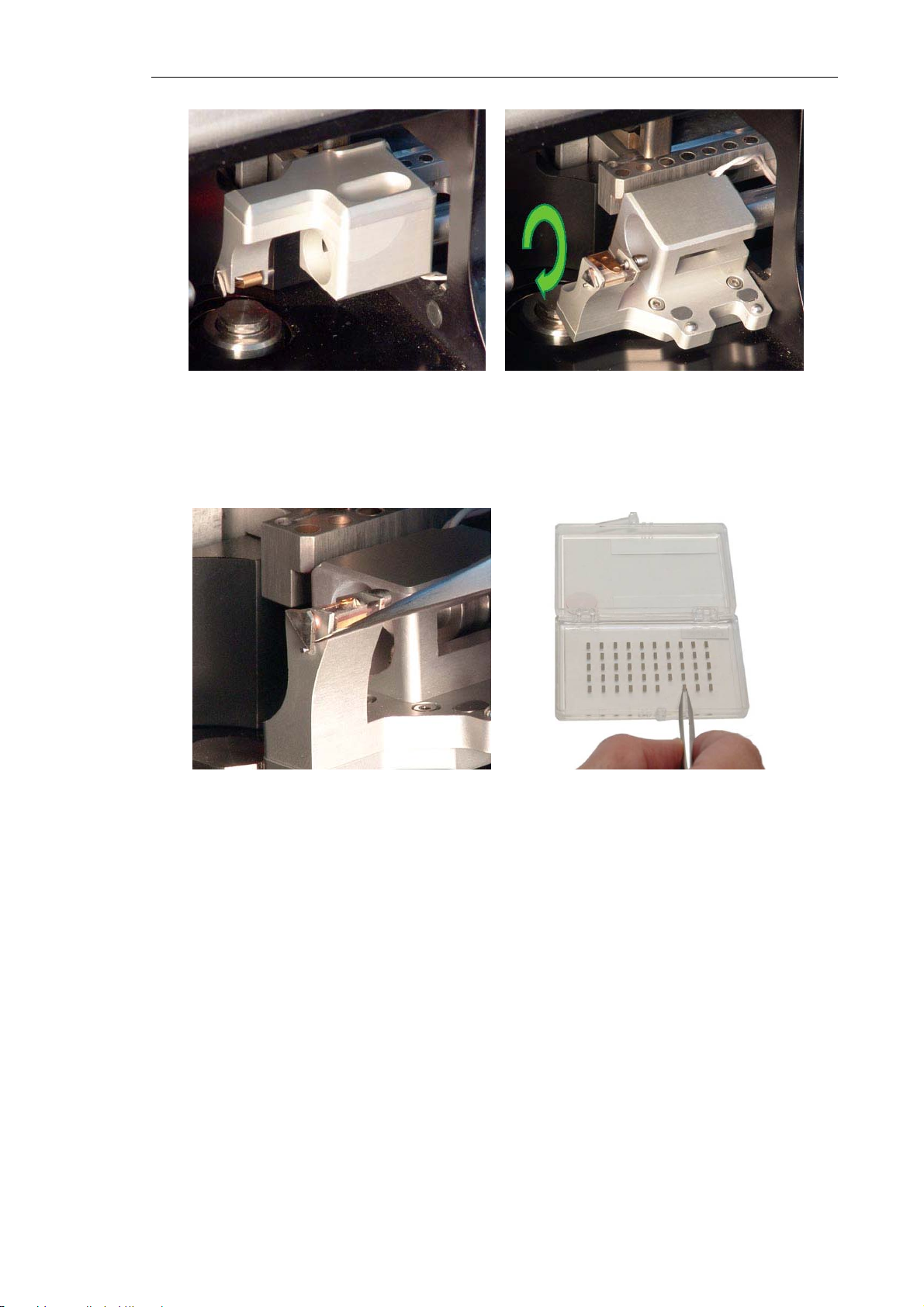
3. Release the probe clip spring by turning downward the trapezoidal lever, located on the
outer side of the holder body, with a tweezers (see Fig. 6-15).
Fig. 6-15 Fig. 6-16
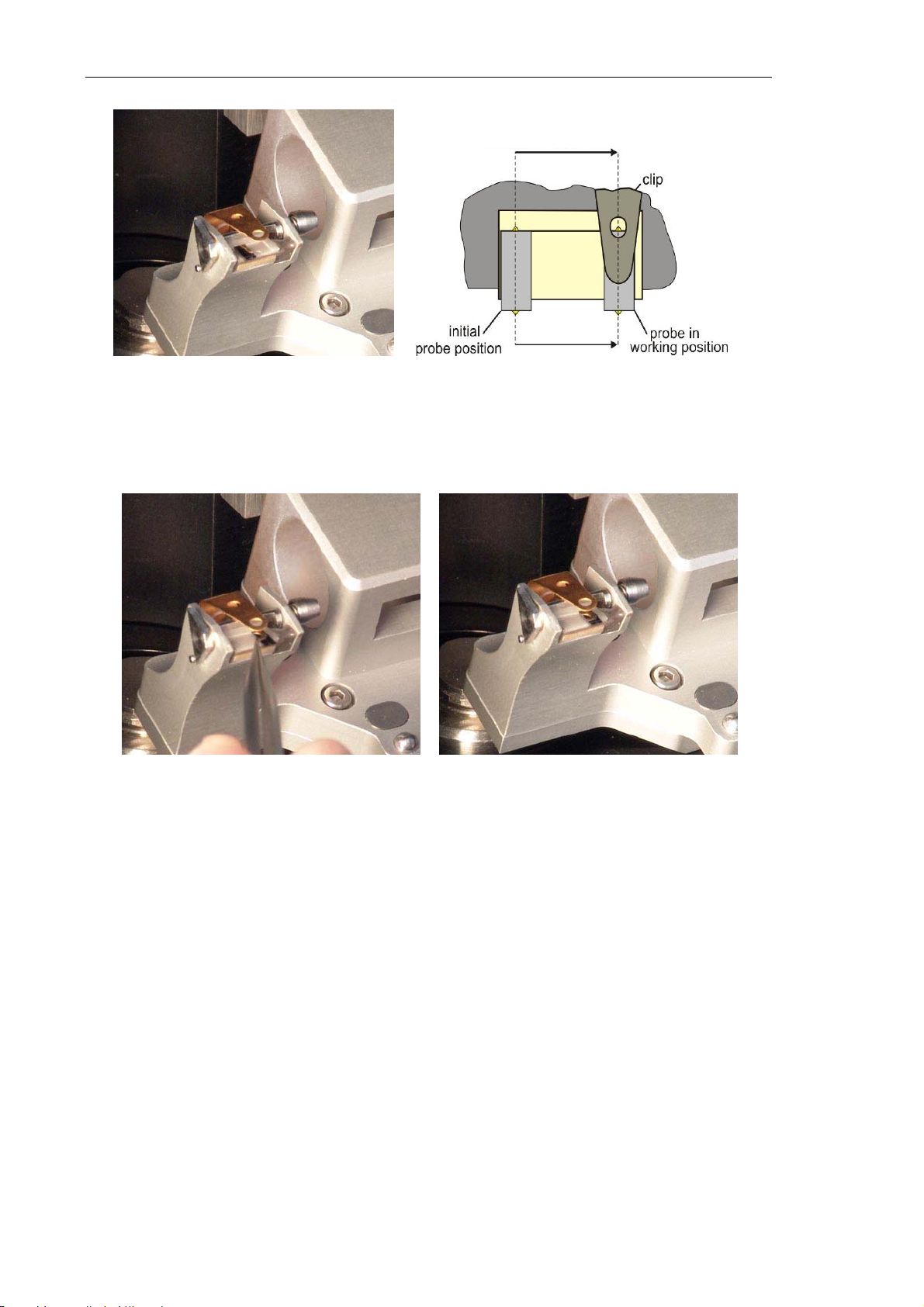
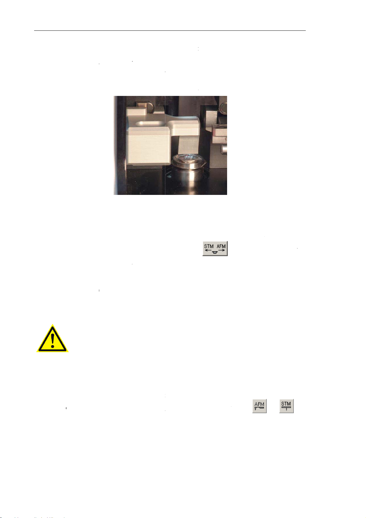
4. Using tweezers, take a probe from the container (see Fig. 6-16). Probes in the container
are placed with their tips pointing upwards. Do not turn the chip over during the
installation.
5. Place the probe on the sapphire pedestal to the left of the working position
(see Fig. 6-17, Fig. 6-18) which is in the right corner under the clip.
35
Page 44
Solver NEXT SPM. Instruction Manual
translation with the tweezers
Fig. 6-17 Fig. 6-18
6. Move the probe with the tweezers to the working position (see Fig. 6-19) as shown
schematically in Fig. 6-18. The probe at its working position is shown in Fig. 6-20.
Fig. 6-19 Fig. 6-20
7. Once the probe is in the working position, clamp it with the clip by turning the lever
counterclockwise to extreme position with the tweezers (see Fig. 6-21).
8. Turn the measuring head to its working position manually (see Fig. 6-22).
36
Page 45
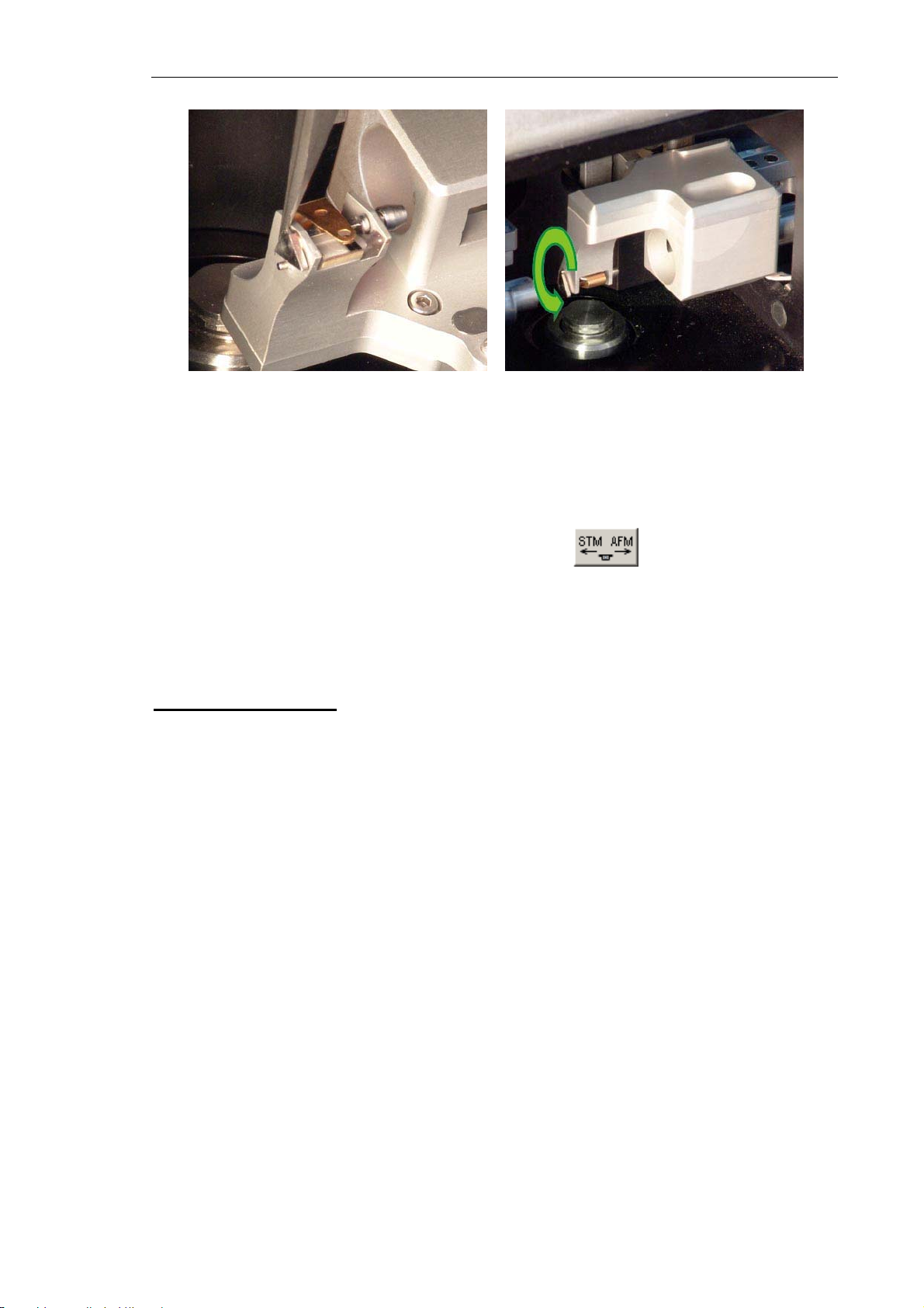
Fig. 6-21 Fig. 6-22
AFM probe is now installed.
Chapter 6. Preparing for Measurements
NOTE. If the AFM probe is not planned to work after installation, it is recommended to
withdraw it to its inoperative position by clicking the button on the Measuring
heads control panel (see Fig. 6-4).
6.4.2. Installing the STM Tip
Manufacturing the Tip
The STM tip is the sharpened end of a piece of platinum-iridium (PtIr), or platinumrhodium (PtRo) (with platinum content of about 80 %) or tungsten (W) wire, 8÷10 mm in
length with a diameter of 0.25÷0.5 mm.
The sharpness of the tip can be estimated by imaging a reference sample with known
surface characteristics, for example, Highly Oriented Pyrolytic Graphite (HOPG).
There are two techniques of manufacturing an STM tip:
1. By cutting the wire apex with scissor (PtIr, PtRo) (see below).
2. By electrochemical etching (W, Pt, PtIr, PtRo).
The simplest STM tip manufacturing technique is cutting the wire apex with the scissors.
This provides the apex radius of curvature less than 10 nm.
Sharp-edged scissors and tweezers with kinks on the interior surface (see the toolkit
supplied with the instrument) are used to cut the wire.
37
Page 46
Solver NEXT SPM. Instruction Manual
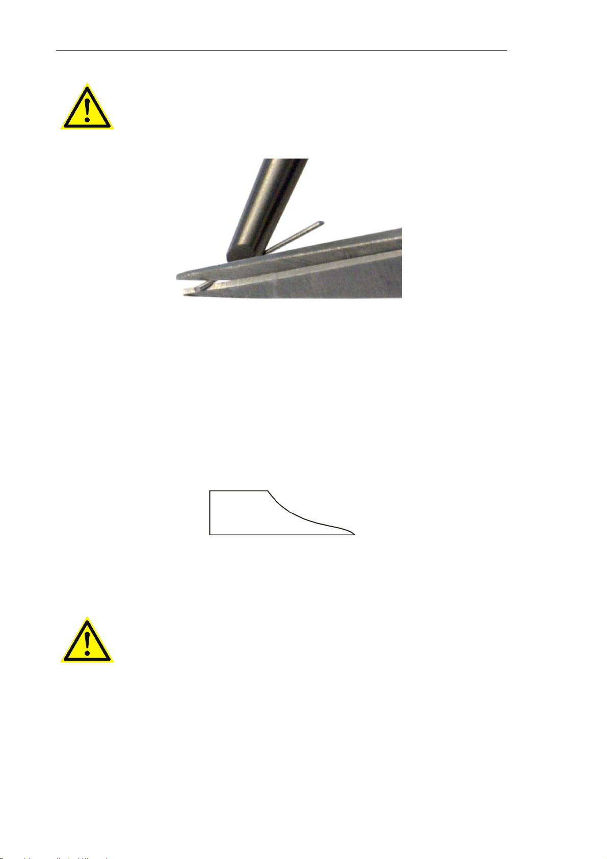
ATTENTION! Do not use the wire cutting scissors for other purposes.
Fig. 6-23
Apex forming procedure includes the following steps:
1. Clamp the wire with the tweezers so that it projects beyond its edge for 2÷3 mm
(see Fig. 6-23).
2. Cut the wire at an angle of 10÷15 degrees as close to its apex as possible and
simultaneously pull the scissors along the wire axis to separate the part being cut off.
This is required to avoid the contact between the cutting edges of the scissors and the
tip apex. Actually, the wire is rather torn off than truncated at the last moment of
contact with the scissor. This results in a sharp apex, formed at the wire’s end
(see Fig. 6-24).
Fig. 6-24. Typical shape of a wire cutoff (apex of the tip)
3. Check the resulting cutoff shape using the optical microscope with 200-x
magnification, if possible. Repeat the cutting process, if necessary.
ATTENTION! Avoid any contact with the tip apex in order not to
damage it.
4. After cutting the wire you may anneal its apex in the flame of an alcohol lamp
for 1÷2 seconds to remove organic substances. Check the apex of the tip using the
optical microscope. The cutoff section should be seen bright, with no trace of carbonblack or dust.
NOTE. The overall length of the tip should not exceed 10 mm.
38
Page 47
I
n
UTo
h
w
e
a
i
e
h
t
a
h
h
h
z
n
T
n
o
r
i
,
a
n
u
t
s
i
h
f
M
h
w
o
(
6
n
o
m
a
h
g
s
2
w
a
h
g
p
F
-
2
d
n
2
e
b
e
n
s
9
g
p
s
e
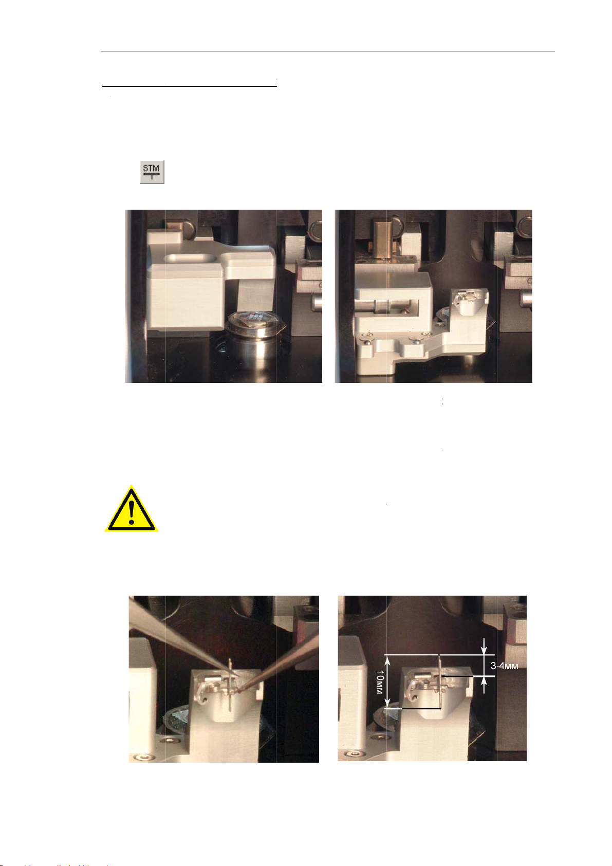
stalling t
e Tip into
he Holde
Ch
pter 6. Pre
aring for M
asurement
se of two t
install or
1.
Move th
the
2.
Turn the
eezers en
exchange t
STM me
button in t
measuring
bles install
e STM tip
asuring he
e Measuri
ead to yo
ng the ST
perform t
d to its
g heads c
manually
tip into t
e followin
orking po
ntrol panel
see Fig. 6-
e holder.
steps:
ition (see
(see Fig. 6
6).
ig. 6-25)
4).
y clickin
3.
Take a p
spring w
Insert th
4.
edge of t
ir of twee
th the seco
ATTEN
during i
tip's blunt
e holder t
Fig.
6-25
ers. Hold
d tweezer
ION! Avo
stallation.
end into t
distance o
he tip with
(see Fig.
d contacti
e holder s
less 3÷4
the first t
-27).
the sh
that the s
m (see Fi
Fig. 6-
eezers an
rpened ap
arpened e
. 6-28).
6
release th
ex with a
d projects
probe cli
surface
beyond th
Fig.
6-27
Fig. 6-
8
3
Page 48
Solver NE
X
e
f
s
h
s
t
i
t
S
H
4
o
r
r
g
p
n
n
l
r
o
s
g
H
N
t
p
h
e
c
u
e
fi
t
t
o
4
)
B
r
o
l
e
p
r
p
g
o
c
)
m
e
e
e
t
g
r
a
a
r
e
M
r
p
c
e
o
b
i
n
g
u
e
c
h
o
a
n
a
i
a
n
p
6
T SPM. Inst
uction Man
al
5. Releas
NOTE.
actor
6. Turn t
STM tip i
the sprin
Tip shar
determini
e measuri
now instal
. Make sur
ness and
g the quali
g head to i
ed.
that the ti
rmness of
y of STM
s working
Fi
is fixed fi
the tip fix
esults.
osition m
. 6-29
mly in the
tion in th
nually (see
holder.
clamp ar
Fig. 6-29).
the prim
ry
NOTE. If
withdraw
heads con
6.5.
(
Procedure
on page 3
With the s
working p
the Measu
he STM p
t to its in
rol panel (
electin
EAD
ATTE
magne
not to
on moving
.
ample at t
sition (se
ing heads
obe is not
perative p
ee Fig. 6-
IPEX™
TION!
ic fastene
revent m
the sample
e extreme
Fig. 6-30)
ontrol pan
planned t
sition by
.
the
Syste
efore sel
should b
vement of
to the extr
ower posi
by clickin
l (see Fig.
work afte
licking th
)
cting the
placed at
the measu
me lower
ion, advan
the corre
6-4).
installati
easur
measuri
its lowest
ing head.
osition is
e the desir
sponding b
n, it is re
utton in t
ng
head,
extreme f
iven in det
ed measuri
tton (
ommended
e Measur
He
the scan
r the sam
il in item
g head to
or )
to
ng
d
er
le
.4
its
in
40
Page 49
Chapter 6. Preparing for Measurements
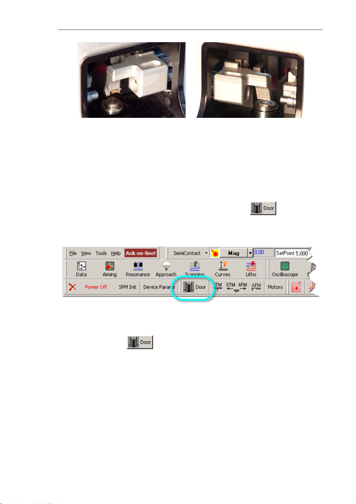
a) AFM head b) STM head
Fig. 6-30. Measuring head at its working position
6.6. Screening with the Protective Shield
(ISOSHIELD SYSTEM™)
To activate screening with the protective shield, click the button in the
Measuring heads control panel (see Fig. 6-31). This draws down the protective shield that
covers the measuring head and the sample to reduce exposure of the measurement system
to external noises thus improving conditions for scanning.
Fig. 6-31
Repeated click on the button lifts the protective shield and opens access to the
measuring heads and to the sample.
6.7. Adjusting the Cantilever Deflection Detection
System
For STM measurements, skip this section and proceed with initial approach (see sect. 6.8
“Initial Approach” on p. 51).
Adjustment of the cantilever deflection detection system is necessary for AFM
measurements. Proper alignment of the detection system requires that the initial laser beam
falls on the cantilever end while the reflected beam comes to the center of the photodiode
and illuminates uniformly all its quarters.
41
Page 50
Solver NEXT SPM. Instruction Manual
NOTE. The laser for detecting the cantilever deflection is kept off while the protective
shield is lifted. The laser is activated automatically after the shield is drawn down.
Two modes are provided for adjusting the cantilever deflection detection system:
● Automatic mode (see sect. 6.7.1 on p. 42);
● Manual mode (see sect. 6.7.2 on p. 43).
Below, these modes are explained in details.
6.7.1. Adjusting the Cantilever Deflection Detection System in
Automatic Mode (EXPERTFBA™ System)
Before aiming the laser beam at the cantilever, the measuring threshold (minimum level)
corresponding to detection of the reflected beam should be defined. The aiming procedure
acquires the laser signal taken by the photodiode in the process of automatic search. When
a point is found where the signal exceeds the threshold, the search region is narrowed and
the photodiode is accordingly repositioned. Optimization of the photodiode position can
take several iterations.
To adjust the cantilever deflection detection system in the automatic mode, perform the
following steps:
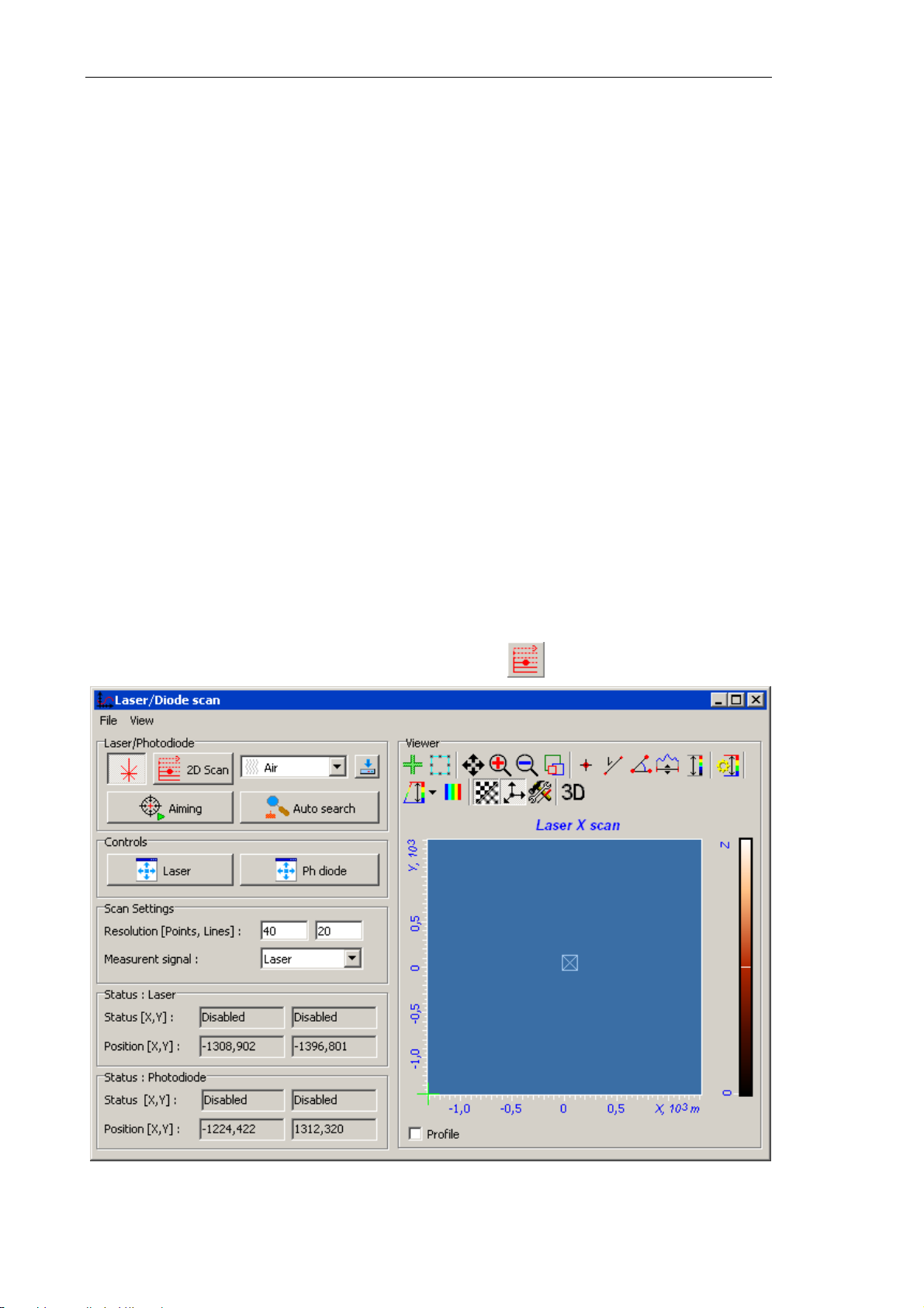
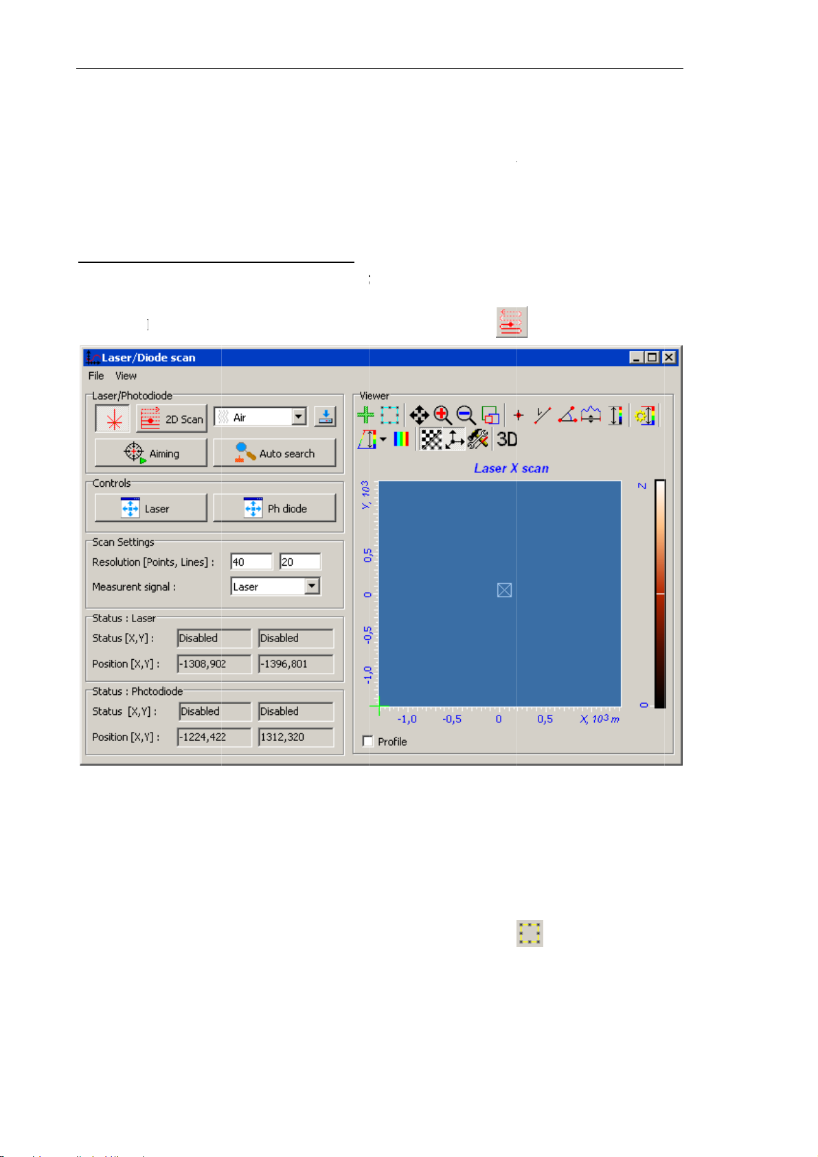
1. Open the Laser/Diode scan window by clicking the button (see Fig. 6-32).
42
Fig. 6-32. Window
Laser/Diode scan
Page 51
2.
c
A
m
o
e
c
l
l
0
t
v
m
o
s
A
M
h
:
h
d
n
fi
.
gs
a
P
c
g
d
m
u
f
o
p
e
d
m
g
M
e
a
i
e
n
e
m
e
e
e
u
o
a
h
p
i
a
F
6
n
t
a
n
a
n
P
a
e
m
n
d
e
n
d
e
h
h
A
r
n
a
n
e
e
m
p
t
e
a
t
g
d
t
w
i
p
c
.
r
n
n
e
b
a
a
i
i
r/
e
a
e
o
o
o
e
r
i
s
z
n
r
y
n
s
3
e
e
d
n
n
t
r
e
e
m
e
e
w
e
n
o
In the m
default s
3.
In the
reflected
4.
In the
prescribe
the scan
input fie
greater 2
5.
In the
adjusting
des droparch regio
T
hreshold
laser beam
S
an Settin
positions
ine in the
d. To redu
.
Si
nal
drop-
the syste
own list of
for the ca
eld of th
It is reco
panel, d
t which th
oints in lin
e the acq
own list
.
the
Laser/
tilever in
Search S
mended to
fine para
laser sig
input fiel
isition tim
f the
Sca
Ch
hotodiode
ir.
ttings
pa
adjust it to
eters of th
al will be t
and numb
, these nu
Settings
pter 6. Pre
panel, sele
el, define
1 or larger
search g
aken. Defi
r of the li
bers are r
anel, selec
aring for M
t
Air
. This
the thresh
id. Points
e number
es in the
commend
t the
Lase
asurement
defines th
ld for th
f this gri
f points i
Li
nes in sca
d to be no
signal fo
6.
Launch
grid and
thus pro
will be
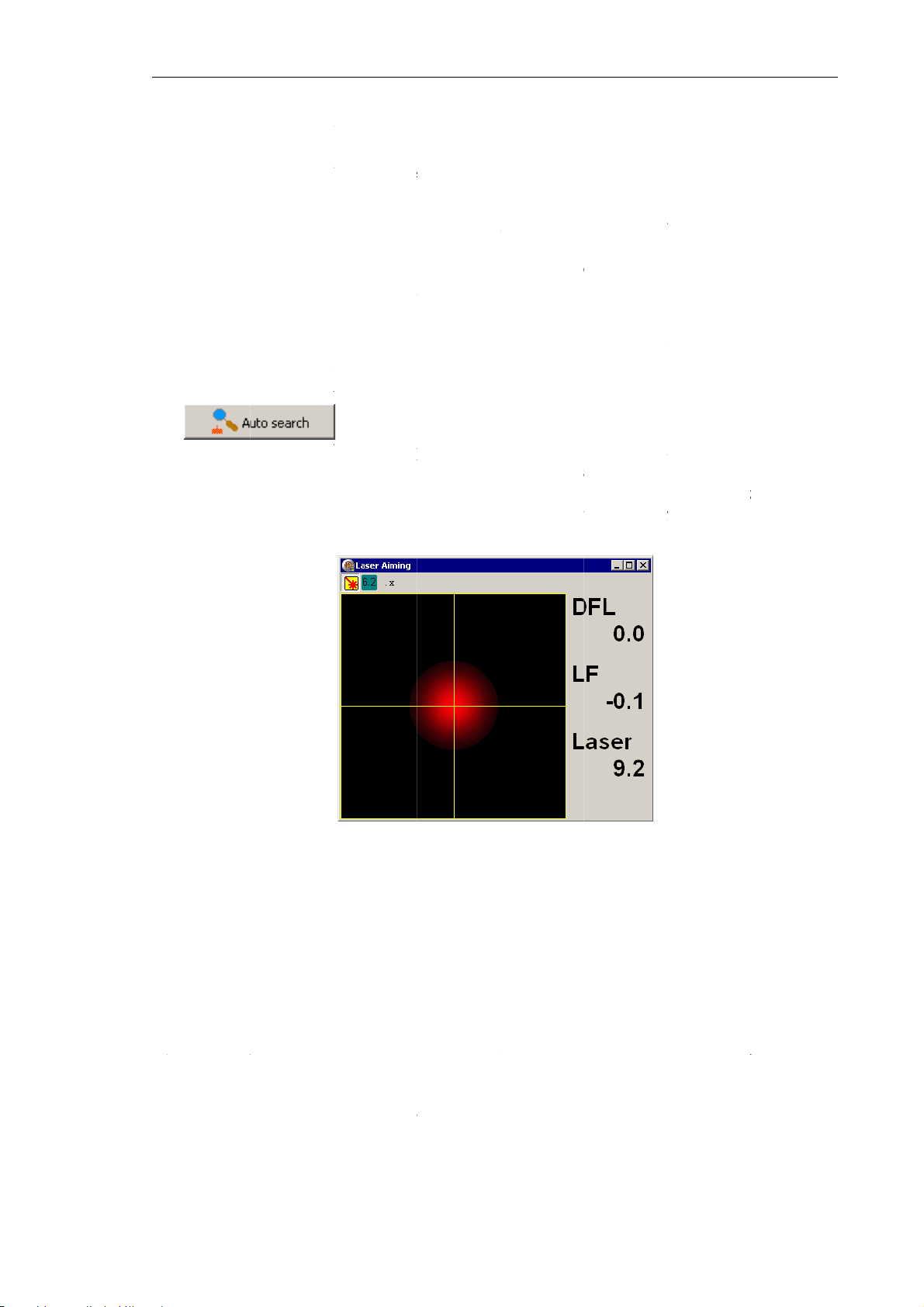
Laser Ai
(see Fig.
he proced
searching
iding the
reposition
ing
win
6-32).
re on se
button. T
r the best
recise aim
d autom
ow (see
rching an
is starts m
osition w
ng of the l
tically. T
ig. 6-33)
aiming
asuring th
ere the det
aser beam
e aiming
and in
he laser
laser sign
ected sign
t the cant
process
he
Lase
eam by c
l line by l
l obtains it
lever. The
s visuali
/Diode sca
icking th
ne over th
maximu
photodiod
ed in th
windo
Fig.
-33.
C
ompletion
S
an proces
f the laser
finished
beam aimi
essage in
Laser
g procedu
he
Laser/D
imin
win
e in the au
iode scan
ow
omatic mo
indow.
de is confi
med by th
6
.7.2.
djusting t
ajor stages
1.
Aiming t
2.
Aligning
B
elow, these
djustin
anual
e cantilev
e laser be
the photod
stages are
the C
ode
r deflectio
m at the c
ode.
xplained i
ntilever
detectio
ntilever;
details.
Deflect
system in
on Det
the manu
ction S
l mode i
stem i
cludes tw
4
Page 52
Solver NE
X
a
p
b
l
h
e
h
m
t
a
r
l
r
v
e
a
m
i
p
i
e
n
u
c
i
d
y
a
t
w
6
c
n
a
.
o
o
d
fo
c
e
n
a
g
e
h
i
l
e
n
d
e
l
o
m
b
v
p
e
n
e
w
i
h
w
n
s
o
e
t
T SPM. Inst
uction Man
al
Actually,
over the
eam bein
The point
where the
Aiming t
To aim th
1. Open t
iming the
redefined
g moved o
of the high
aser beam
e laser be
laser bea
e
Laser/D
aser is pre
egion. Th
er the pre
st intensit
is then dire
m at the c
at the can
ode scan
eded by c
s acquisiti
efined gri
in the col
cted.
ntilever
ilever, per
indow by
llecting th
n is perfo
and the p
lected distr
rm the fol
licking th
distributi
rmed auto
otodiode
bution pro
owing ste
button
n of the r
atically,
eing the si
ides posit
s:
(see Fig.
flected sig
ith the la
gnal detect
on of inter
6-34).
al
er
r.
st
Fig.
-34.
Laser/
2. In the
defaul
3. Define
a. En
44
odes dro
search reg
the region
ble the Ar
the
Viewer
-down list
on for the
for searchi
a moving
pa
el (see Fig
of the
antilever i
g for the c
nd resizin
6-35).
Las
Diode sca
r/Photodio
air.
ntilever (s
tool by c
window
e
panel, s
arch regio
icking the
lect
Air
) as follo
button
. T
is defines
s:
on the top
he
of
Page 53
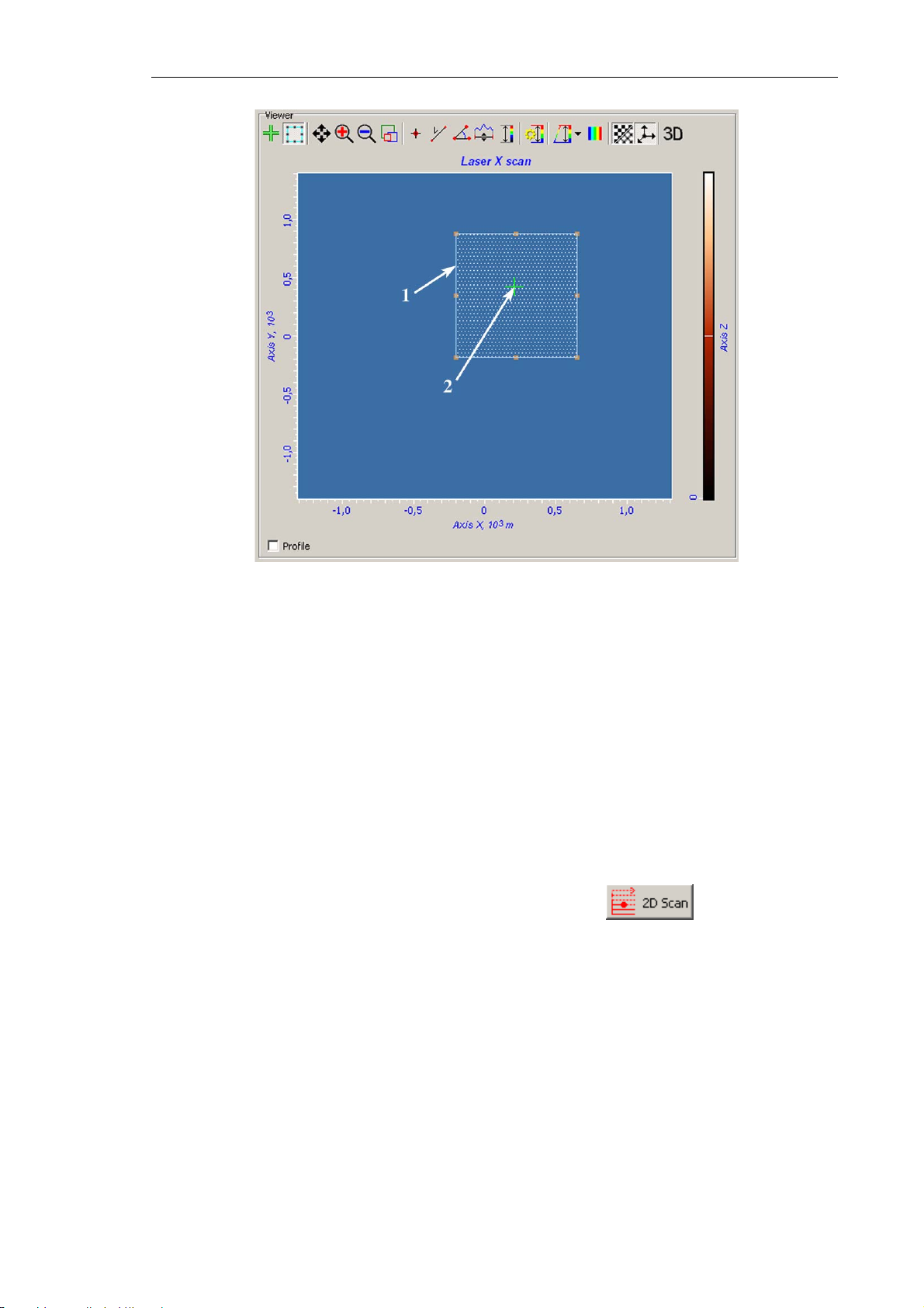
Chapter 6. Preparing for Measurements
Fig. 6-35.
1 – boundary of the selected search region;
2 – cursor pointing to the laser beam position
Viewer panel
b. Move and/or resize the search area with the mouse (see. 1 on Fig. 6-35).
4. In the Scan Settings panel, define parameters of the search grid. Points of this grid
prescribe positions at which the laser signal will be taken. Define number of points in
the scan line in the Points in line input field and number of the lines in the Lines in scan
input field. To reduce the acquisition time, these numbers are recommended to be not
greater 20.
5. In the Signal drop-down list of the Scan Settings panel, select the Laser signal for
adjusting the system.
6. Start the procedure on searching the laser spot with the button. This starts
measuring the laser signal line by line over the grid and displaying the image acquired
by the photodiode in the 2D Viewer.
The measuring completes resulting in one of two following situations:
● The laser spot is caught and displayed in the Viewer (see Fig. 6-36). In this case, go
to step 7 for improved positioning of the laser spot;
● The Viewer misses the laser spot. This means that the cantilever is outside of the
search region or photodiode fails to catch the spot. You have either to enlarge the
search region and then to repeat steps 2-4 or to reposition the photodiode.
45
Page 54
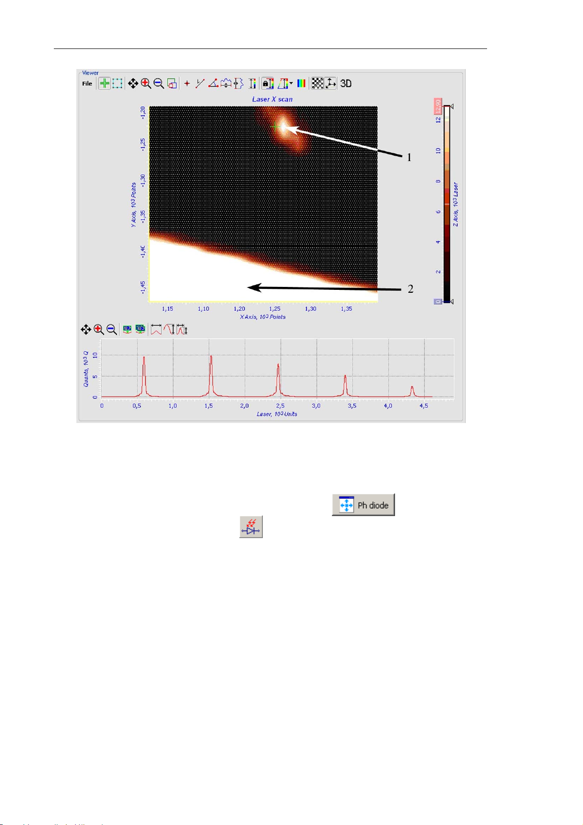
Solver NEXT SPM. Instruction Manual
Fig. 6-36. 2D Viewer
1 – laser spot from the cantilever; 2 – laser spot from the chip
For repositioning the photodiode, click the button of the
Laser/Diode scan window or the button of the stepper motor control panel to
open the
control buttons of the
laser spot. Monitor the laser spot in the
Diode mover window (see Fig. 6-37). Switch to the Manipulator tab. With the
XY Controls panel, move the photodiode so that it detects the
Laser Aiming window (see Fig. 6-40). When
the spot becomes visible, repeat steps 2-4.
46
Page 55
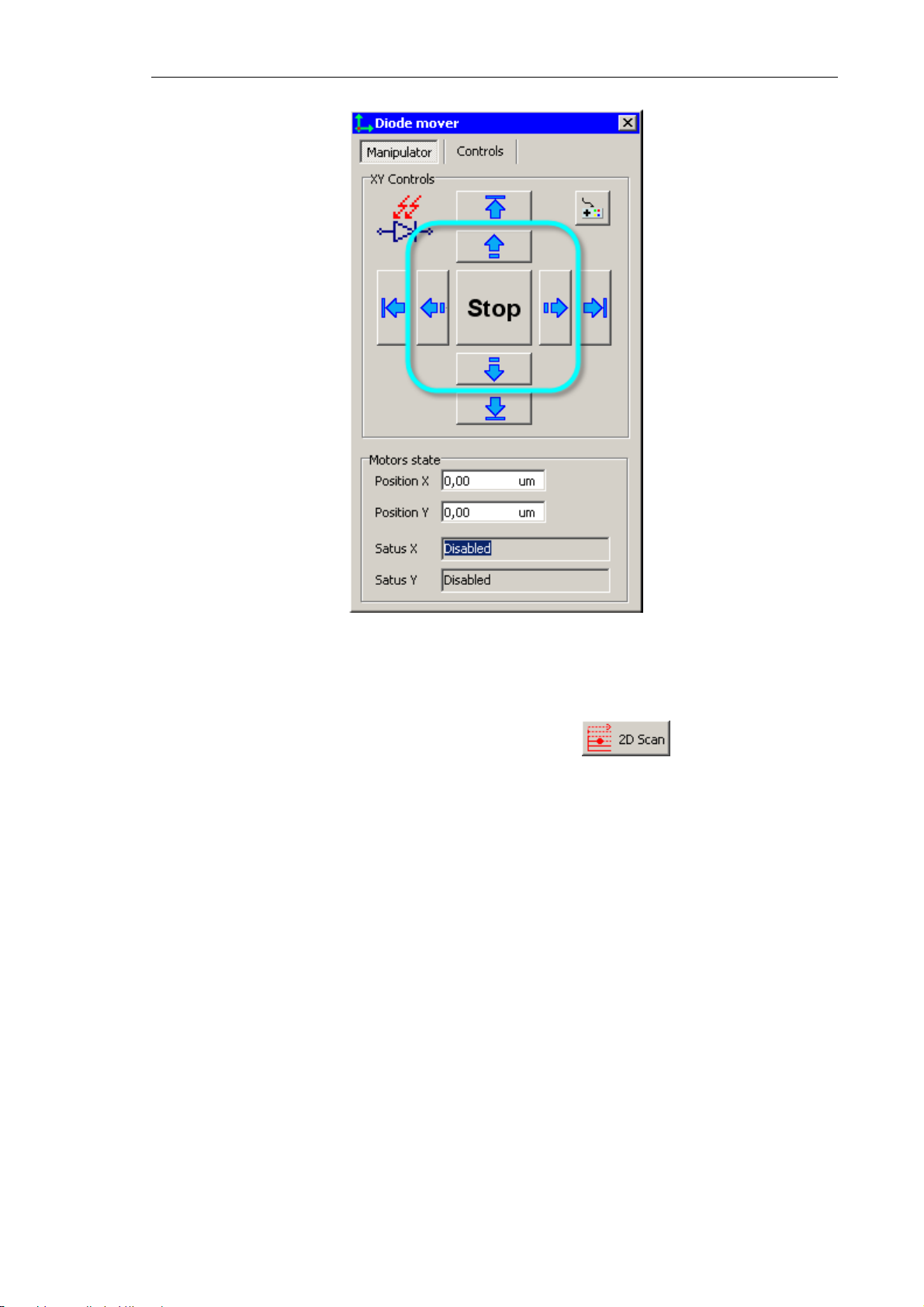
Chapter 6. Preparing for Measurements
Fig. 6-37.
Diode mover window. Photodiode position control tab
7. Repeat acquisition of the laser spot intensity distribution over a small region around the
previously found position of the spot by clicking the button. This provides
more precise profile of the distribution over the narrowed region that is displayed in the
2D Viewer (see Fig. 6-38). Acquisition of the laser spot distribution finishes. Now the
beam is to be aimed at the cantilever.
47
Page 56
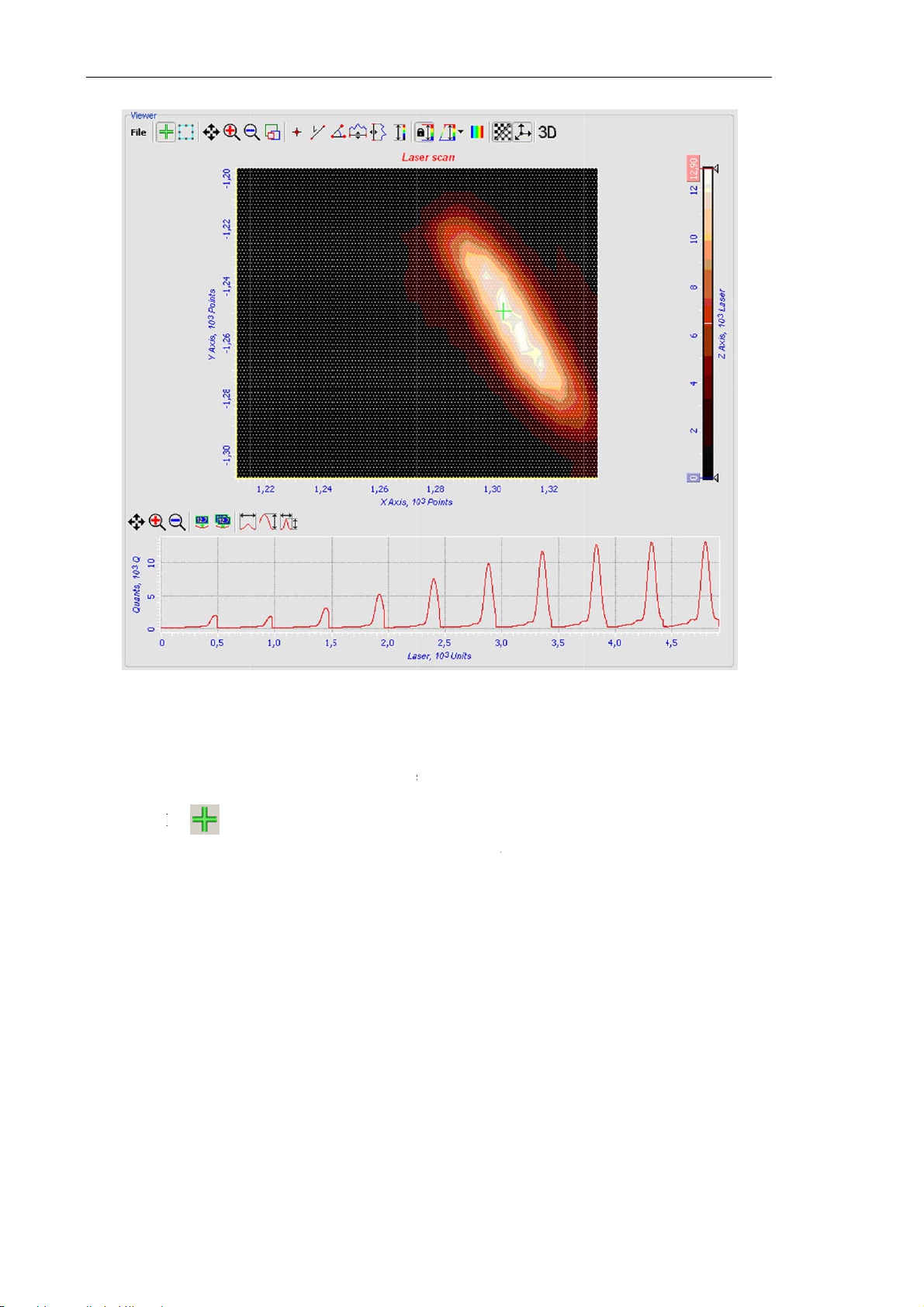
Solver NE
X
e
h
t
c
rFi
m
t
a
-
m
u
f
b
s
y
e
s
e
i
g
r
t
l
t
d
w
e
n
o
e
o
n
c
t
t
i
T SPM. Inst
uction Man
al
To aim th
1. Click t
2. Move
mouse
3. Open
Move t
to the
laser bea
e but
he cross-h
(see Fig. 6
the contex
o probe
ite
ursor.
g. 6-38. Pro
at the pro
on on the t
ir cursor (
38).
t menu b
in the m
ile of the la
e cantilev
op of the
ee 2 on Fi
clicking
nu. The la
er spot afte
r, perform
V
ewer
pane
. 6-35) to
the secon
ser beam
repeated s
he followi
(see Fig. 6
he center
ary mous
ill move t
arch
g steps:
-38).
f the laser
button a
the point
spot with
d select
orrespond
he
he
ng
48
Page 57
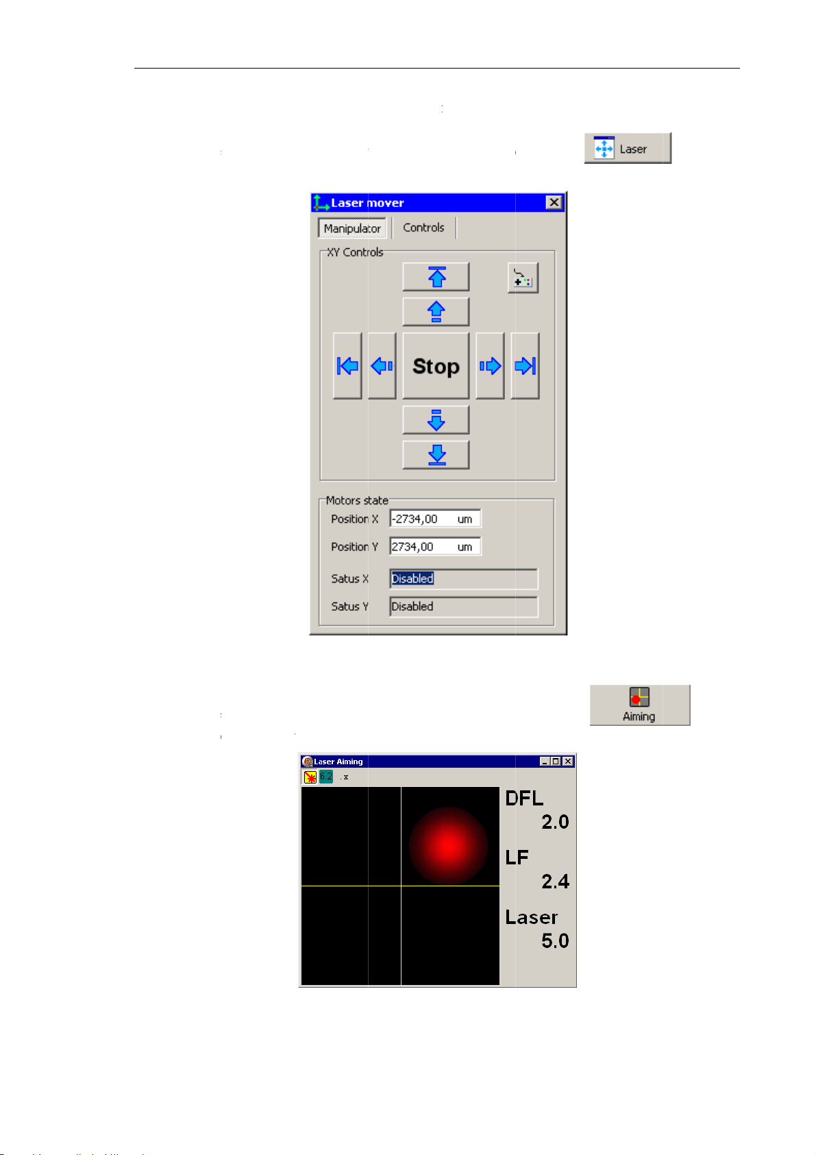
T
o
a
e
r
e
p
t
v
-
r
v
w
S
Ming
w
6
r
6
h
o
6
t
A
a
n
c
a
s
m
d
p
h
n
e
n
s
9
n
n
aim the l
1.
Open th
the
Lase
ser spot at
Laser mo
/Diode sca
he cantile
er
windo
n
window.
er with mo
(see Fig.
witch to t
Ch
e precisio
-39) by cli
e
Manipul
pter 6. Pre
, perform t
king the
tor
tab.
aring for M
e followi
asurement
g steps:
button i
2.
Open th
in the
Laser Aim
O
eration Fo
Fig. 6
39.
windo
ms
toolbar
Laser
Fig.
over
wind
(see Fig.
of the Con
-40.
Laser
w. Laser po
-40) by cl
rol Progra
iming
win
ition contro
icking the
Main Wi
ow
l tab
dow.
butto
4
Page 58
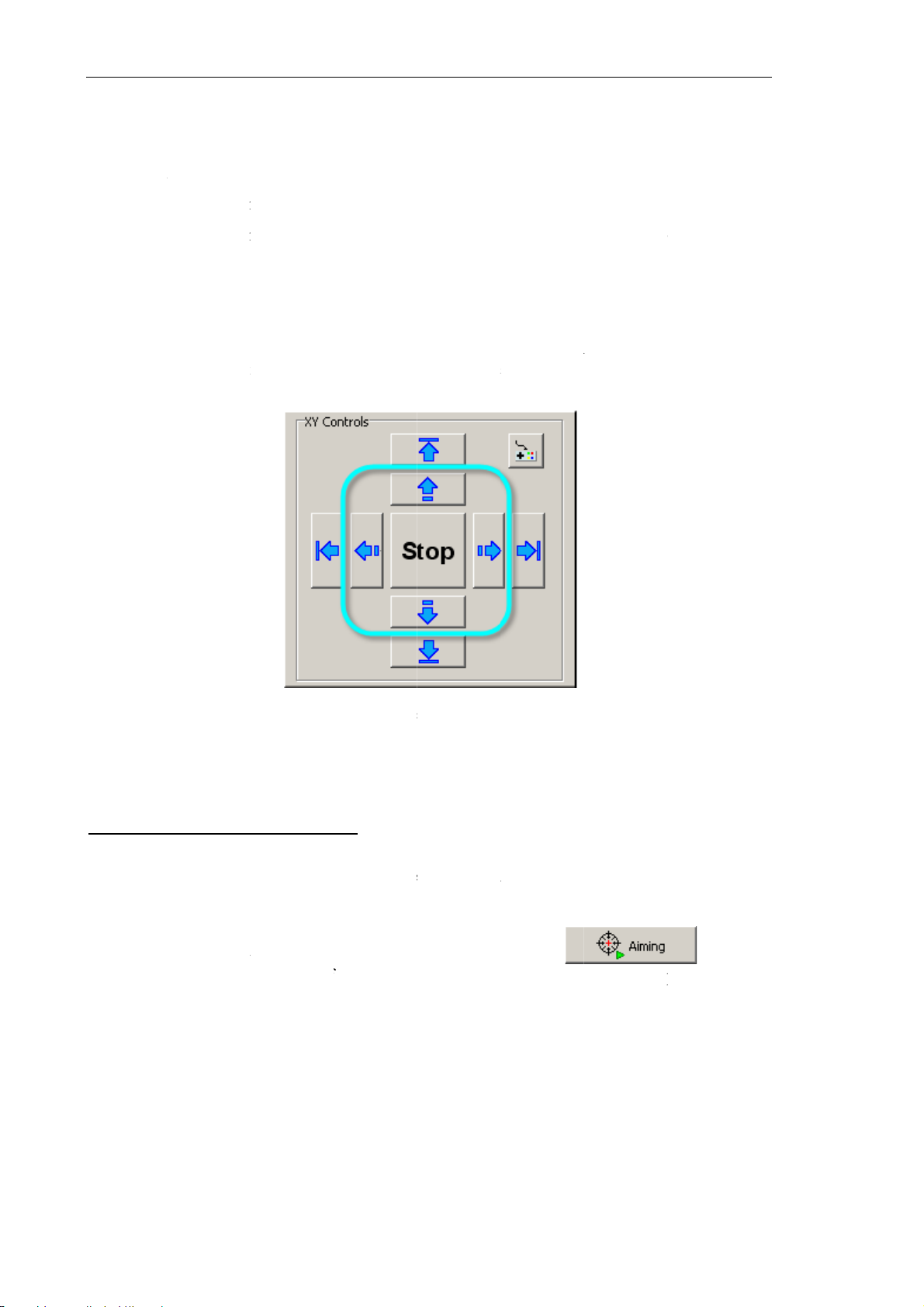
Solver NE
X
a
o
a
o
b
a
b
P
i
r
g
c
t
n
n
s
t
w
d
a
a
g
w
u
a
n
n
i
i
e
e
f
6
2
e
n
f
A
s
e
e
h
D
s
f
w
o
g
d
s
d
d
c
m
i
o
h
m
a
s
m
M
d
o
o
i
s
o
p
s
i
t
t
The
the ph
T SPM. Inst
L
ser Aimin
todiode se
uction Man
window c
tions (left)
al
ontains a
and a tabl
D Viewer
of current
howing i
levels of th
age of the
e photodio
laser spot
e outputs.
on
The v
DFL
LF
Laser
3. Monit
the mo
lues indica
– differe
– differe
– total
intensity
r the
Lase
vement bu
ed in the t
ce betwee
ce betwee
um of all
reflected b
r
signal in
tons (see F
ble corresp
the upper
the left a
sections o
y the cantil
the
Laser
g. 6-41) so
ond to the
and the lo
d the right
the phot
ever.
imin
win
that the
La
ollowing s
er halves
halves of t
diode that
ow and
er
signal
gnals:
f the phot
e photodi
is proport
ove the la
chieves its
diode;
de;
onal to la
er beam w
maximum.
er
th
The laser
Adjusting
With the l
reflected
quarters.
To launch
the
Laser/
Laser Aim
Fig. 6
eam is no
the photo
ser beam
eam come
the autom
hotodiode
n
windo
-41. Buttons
aimed at t
iode posit
imed at th
s to the c
tic alignme
Toolbar o
(see Fig.
for step-by-
he cantilev
on
cantilever
nter of th
nt of the p
the
Laser/
-42).
tep movem
r.
, the photo
photodio
otodiode,
iode scan
ent of the la
iode shoul
e and illu
lick the
window.
er beam
d be positi
inates uni
onitor the
ned so as
formly all
button
rocess in
he
its
in
he
50
Page 59
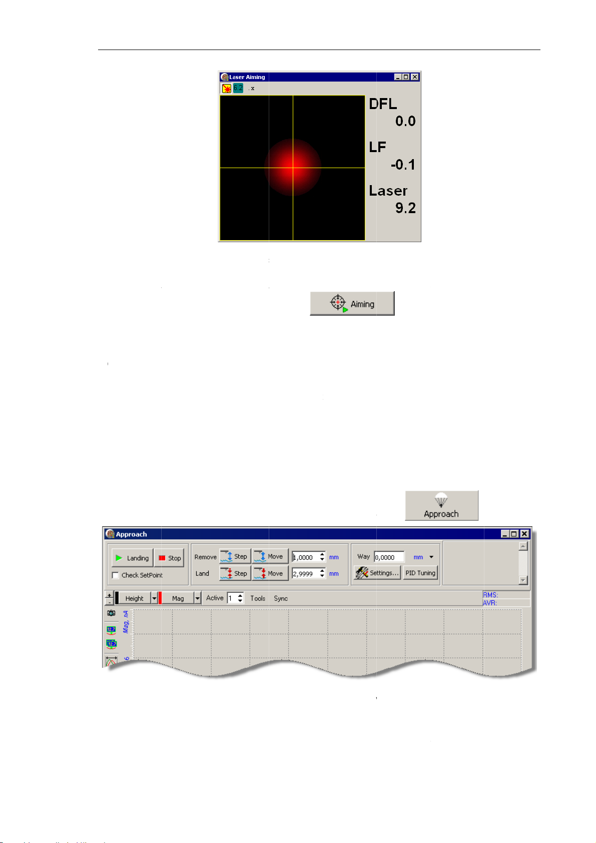
h
e
6
hsadesa
o
u
h
i
a
c
c
h
p
F
m
p
a
p
p
w
r
s
n
a
h
t
r
e
a
w
t
a
r
o
)
Appr
b
p
Ch
a
d
n
s
o
e
n
w
d
p
t
.
1
w
n
h
e
e
o
b
d
s
t
s
e
e
e
pter 6. Pre
aring for M
asurement
T
e proced
c
ntered at t
.8. In
T
e sample
fe for sele
sired area
mple surfa
T
perform t
1.
Open the
re on auto
e photodio
tial Ap
pproaches
ting the sc
under the
e.
e initial a
Approach
ig. 6-42. La
atic alig
de and rele
roach
initially to
n area wit
robe. Safe
proach, pe
indow (s
er spot cen
ment of th
ses the
the probe
the optic
y means p
form the f
e Fig. 6-43
tered at the
e photodio
o the dista
l viewing
eventing c
llowing st
by clicki
photodiode
e comple
button
ce of 0.5÷
ystem and
ntact bet
ps:
g the
es with th
mm. This
for further
een the pr
laser spo
distance i
moving th
be and th
utton.
Fig
. 6-43.
2.
Looking
Control
from the f
anel of the
ont, estim
Approach
te the pro
indow, in
oach
windo
e-surface
ut a value
istance. I
less than t
the
Land
e estimate
field in th
one.
51
Page 60
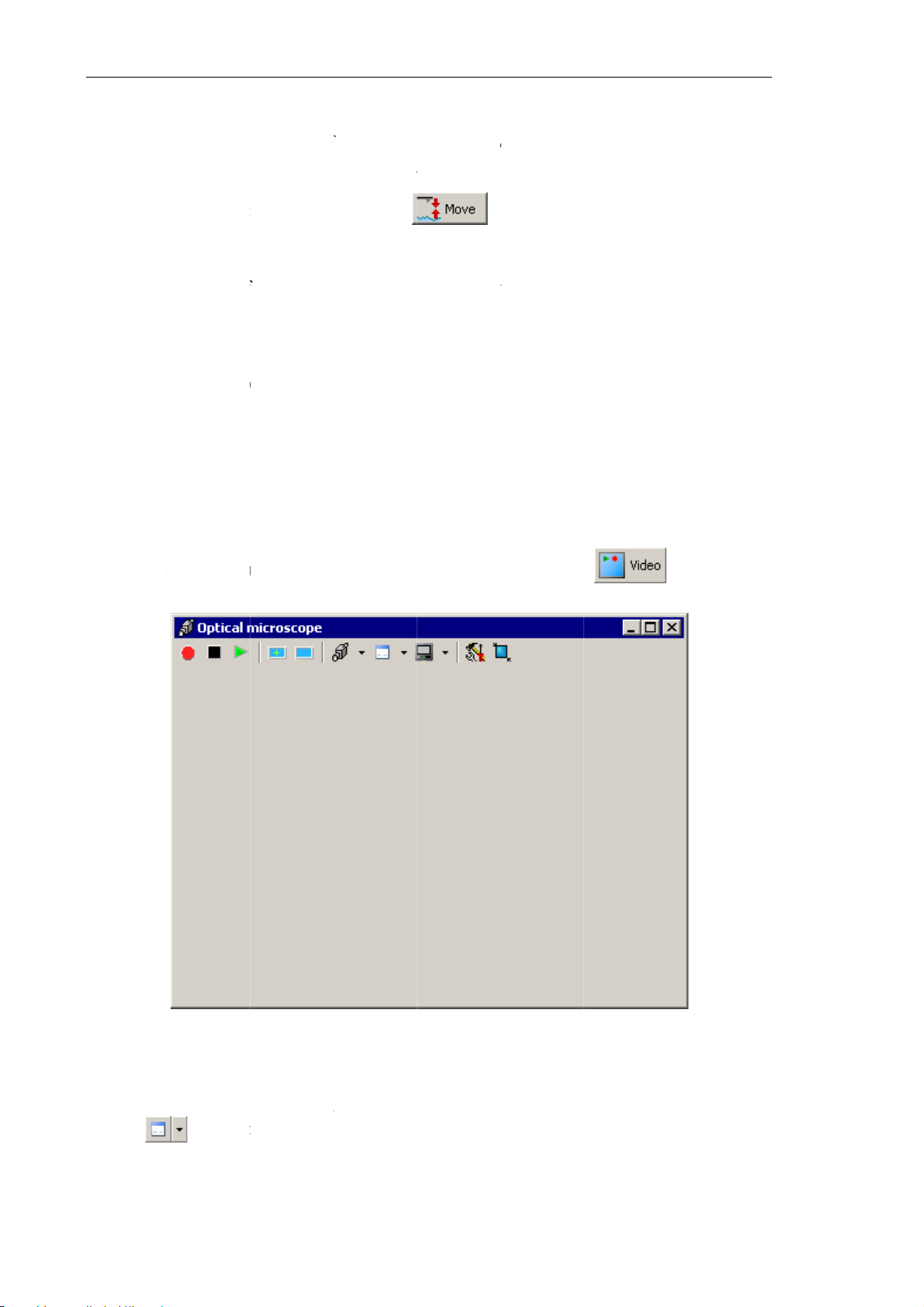
Solver NE
X
t
a
h
c
d
m
e
S
h
h
t
s
t
r
s
n
b
o
f
t
g
l
m
W
P
n
u
p
fa
6
p
g
c
p
o
e
d
d
b
e
c
g
.
d
e
e
s
d
p
e
do
g
P
b
h
t
P
i
4
h
e
o
l
r
S
h
p
T
™
g
w
e
i
m
d
h
p
n
n
l
i
u
t
t
p
t
b
t
T SPM. Inst
uction Man
al
NOTE.
inspec
initial
3. Launc
distan
the vi
4. On co
surfac
6.9.
The simpl
probe wit
To select t
1. Open
Mover
During th
ion of the
pproach (
approachi
e defined
eo microsc
pletion o
. If this dis
electin
est way to
the optica
e area for
he
Optical
panel.
e initial a
probe-sur
ee sect. 6.
g the sam
y the
Land
pe.
approach,
ance is lar
the S
select the
image dis
investigati
icroscop
proach ke
ce distan
“Screenin
le by the
parameter
check the
er 1 mm, r
an Ar
scan area
layed in th
n, perform
window (
p the prot
e. Draw
with the
Observe t
istance be
epeat steps
a (PIN
is through
Optical m
the follow
ee Fig. 6-
ctive shie
wn the p
rotective
utton. This
e approac
ween the
2-3.
OIN
positionin
icroscope
ng steps:
4) with th
d lifted to
otective s
hield” on
moves the
process i
robe tip a
Syste
the samp
indow.
enable vis
ield after
. 41).
sample to
the image
d the sam
m)
e against
utton in
al
he
he
of
le
he
he
Fig. 6-44.
indow for
isplaying th
e image of t
e Optical V
ewing syste
m
2. Open
the
52
he
Video
button i
roperties
the Tool
ialog for a
ar of the
justing th
O
tical micr
video ca
scope
win
era (see F
ow.
g. 6-45) w
th
Page 61
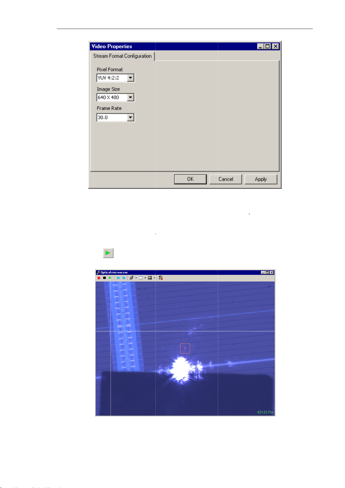
h
a
d
t
l
b
t
p
6
Ad
i
d
T
o
a
a
v
h
Ch
a
e
e
m
.
n
p
c
o
e
e
v
r
T
s
3
e
y
w
pter 6. Pre
aring for M
asurement
3.
Define t
Frame R
4.
Click the
5.
Launch
clicking
will disp
e frame ra
te
list.
OK
utton
isplaying
he but
ay the sam
Fig. 6-45.
te of the v
to save mo
he image
ton in the
le surface
justing dial
deo camer
ifications
from the
oolbar of t
and the pro
g of the vid
to be 30
nd to clos
ideo came
e
Optical
be (see Fig
o camera
Hz by sele
the
Video
ra of the
icroscope
6-46).
cting this
Properties
ptical mic
window.
alue in th
dialog.
oscope b
he windo
Fig.
-46. Viewin
g the image
of the built-i
video cam
ra
5
Page 62
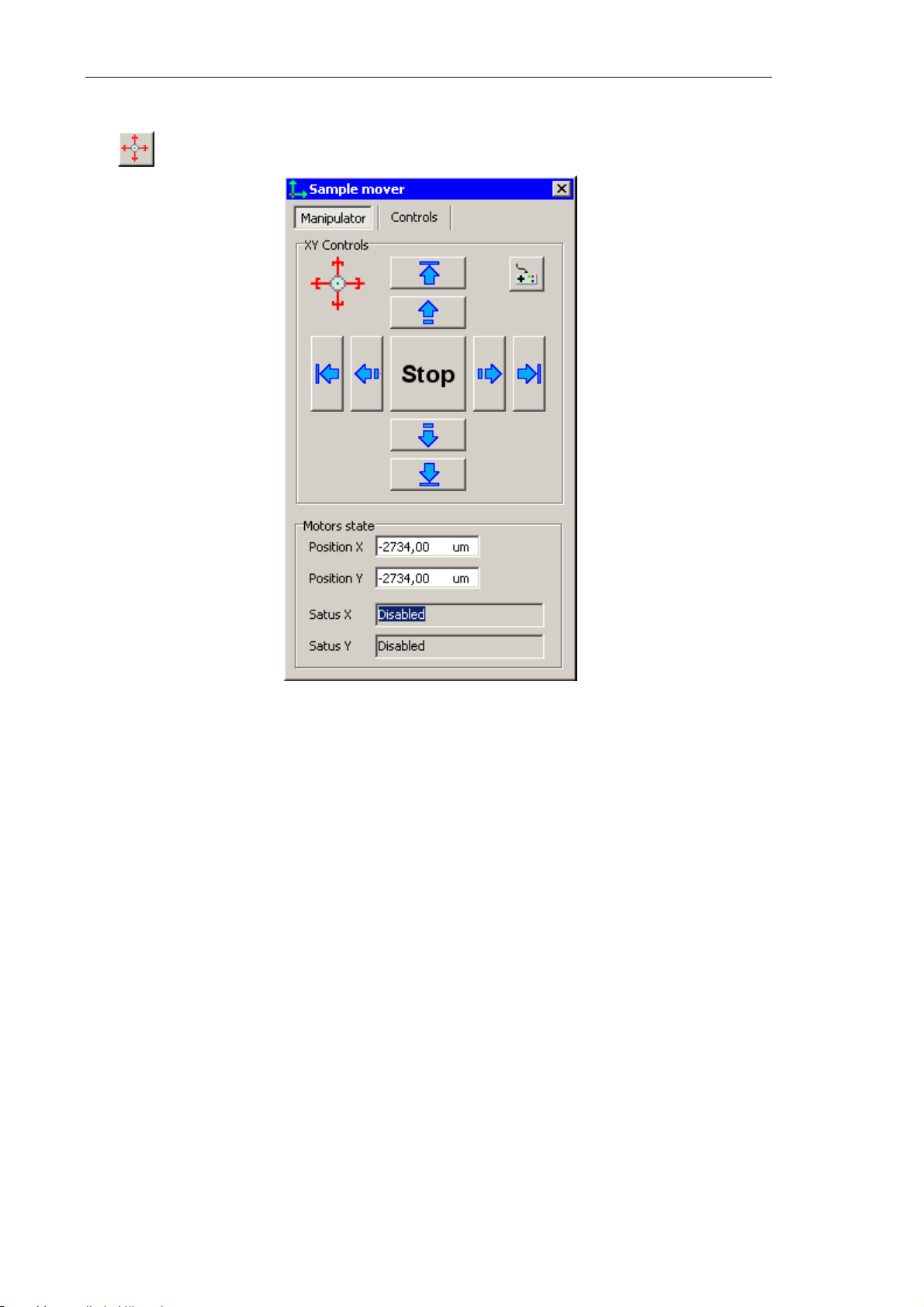
Solver NEXT SPM. Instruction Manual
6. Open the Control window of the sample movement stepper motors by clicking the
button (see Fig. 6-47).
Fig. 6-47. Control window of the sample movement stepper motors
7. Use buttons of the Controls XY panel to move the sample so that the desired area
comes under the tip.
54
Page 63

Chapter 7. Performing Measurements
7. Performing Measurements
7.1. Contact AFM
7.1.1. Constant Force Mode
Operations performed in measurements of surface topography with the Constant Force
Mode have much in common with those of other contact techniques, including the Lateral
Force Mode, the Spreading Resistance Imaging Mode, the Force Modulation Mode, and
the Contact Error Mode.
Initial state
The following steps are assumed to be done:
● Launching the control program;
● Turning the instrument on;
● Installing the probe;
● Adjusting the cantilever deflection detection system;
● Mounting the sample;
● Moving the measuring head to its working position;
● Initial approach;
● Selecting the scan area.
For details on these operations see Ch. 6 “Preparing for Measurements” on p. 29.
Procedural Sequence
Measurement in the Constant Force mode is arranged in the following procedural
sequence:
1. Adjusting the Controller Configuration (see i. 7.1.1.1 on p. 56).
2. Adjusting Initial Level of the DFL Signal (see i. 7.1.1.1 on p. 56).
3. Approaching the Sample to the Probe (7.1.1.2 on p. 56).
4. Adjusting Working Level of the Feedback Gain (7.1.1.3 on p. 58).
5. Adjusting Scanning Parameters (see i. 7.1.1.4 on p. 60).
6. Scanning (see i. 7.1.1.5 on p. 62).
7. Saving Measurement Data (see i 7.1.1.6 on p. 66).
8. Completing Measurements (see i 7.1.1.7 on p. 70).
These procedures are explained below.
55
Page 64
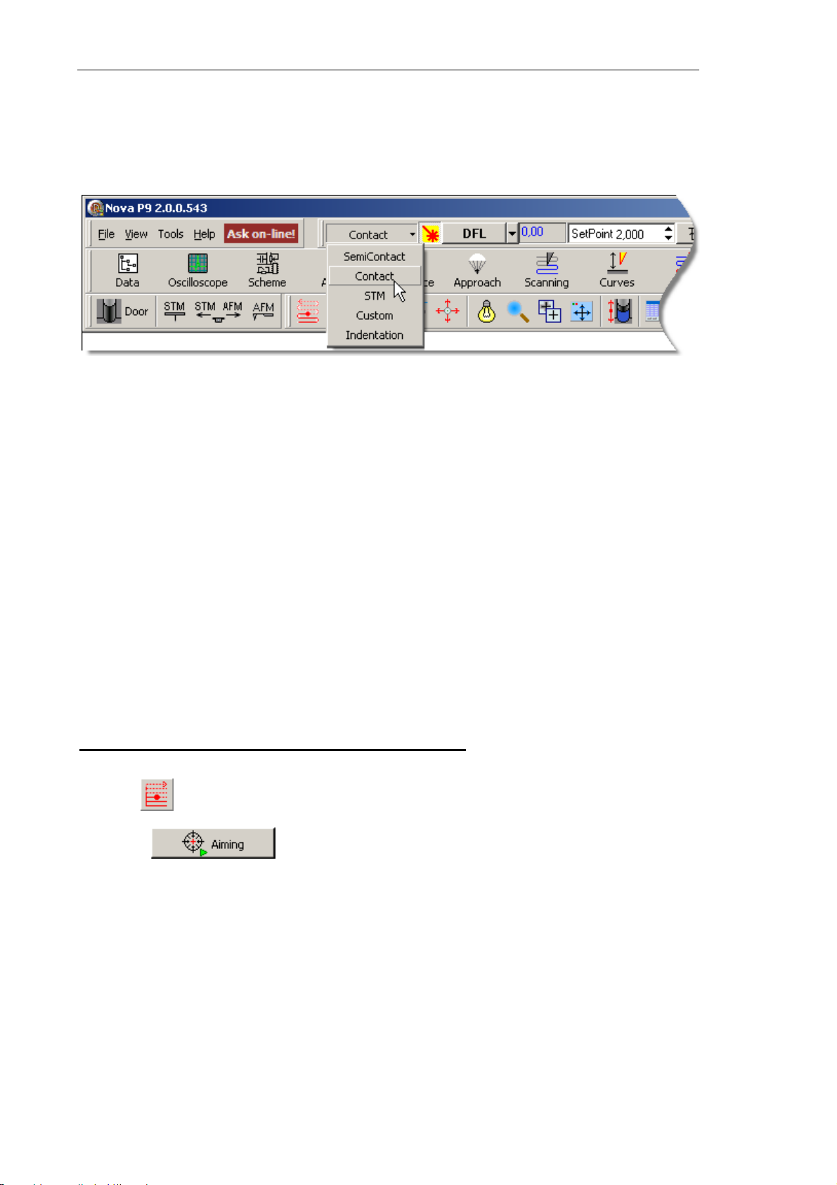
Solver NEXT SPM. Instruction Manual
7.1.1.1. Adjusting the Controller Configuration
Switch the instrument for operating in the Contact technique by selecting Contact in the
controller configuration list (see Fig. 7-1) at the top bar of the Main Program window.
Fig. 7-1. Selecting the controller configuration
Once the configuration Contact is set, all switching sequences required for the instrument
to operate in contact modes proceed automatically.
7.1.1.2. Adjusting Initial Level of the DFL Signal
Initial level of the DFL signal corresponds to the state of the cantilever oscillating freely.
Its value depends on the photodiode position relative to the cantilever reflected beam. The
DFL level is zero when the laser spot is halved by the top and the bottom parts of the
photodiode, that is, the corresponding integral intensities are equal.
Initial level of the DFL signal can be adjusted either automatically or manually.
Adjusting initial level of the DFL signal automatically
Automatic adjustment of the DFL signal uses the
with the button.
Click the button. This launches the photodiode movement motors and
the photodiode will be repositioned so as the laser spot is centered at the photodiode and
the DFL level is close to zero.
Laser/Diode scan window that opens
The Laser Aiming window displays the adjusting process (see Fig. 7-2).
56
Page 65
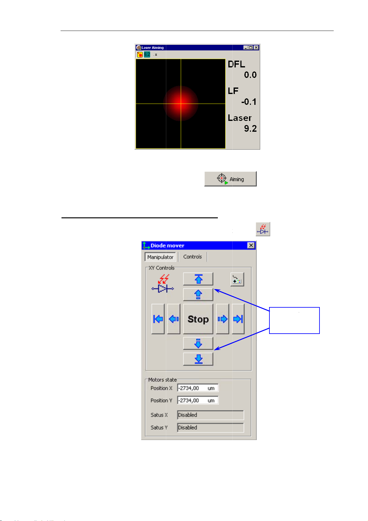
A
o
n
t
o
v
s
o
t
e
n
-
m
C
p
k
o
hapter 7. P
e
bu
e
e
f
s
7
rforming M
asurement
O
n completi
djusting i
1.
Open the
n of adjus
itial level
Diode mo
Fig. 7-2. La
ing the ph
f the DFL
er
window
er spot cen
todiode, th
signal ma
(see Fig. 7
ered at the
ually
3) by clic
hotodiode
ing the
tton releas
button.
Controls
adjusting
s.
or
DFL
Fig.
7-3.
Diode
over
wind
w
5
Page 66
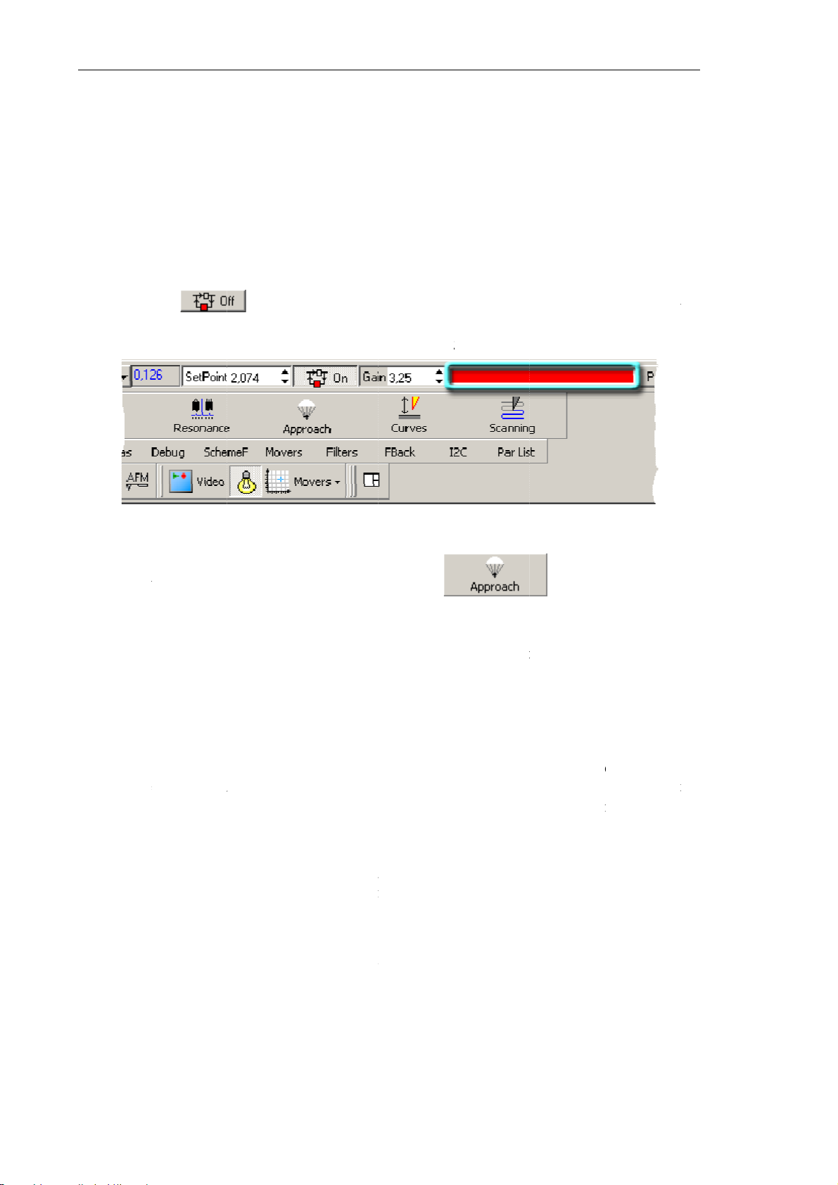
Solver NE
X
o
b
e
c
c
t
i
a
t
m
a
f
e
fpre
tcor
tcor
r
f
b
a
r
o
p
Z
s
A
a
i
f
h
t
e
e
u
a
n
o
r
n
o
l
l
f
u
s
t
t
t
o
t
7
w
t
h
t
P
h
s
h
r
e
s
e
e
u
o
a
L
s
o
a
p
m
m
.
k
n
t
S
r
n
d
n
t
n
w
a
n
e
o
e
w
o
g
o
a
F
d
a
n
o
d
m
e
l
e
e
s
e
e
n
t
r
D
a
e
r
e
e
n
w
v
s
p
s
i
t
w
s
b
e
n
i
)
o
o
v
z
a
a
O
v
h
t
t
e
h
h
i
h
T SPM. Inst
uction Man
al
2. Watch
the sp
etwe
accura
7.1.1.3.
To approa
1. Press
extens
the Sc
position o
t with the
n the top
y of cente
Appr
h the sam
he
on of the
nner exten
the laser
uttons of
nd the bot
ing of the l
aching
le to the pr
button
scanner t
ion indica
pot in the
he
Control
om parts
aser beam
he Sam
obe, perfor
in the top
its maxi
or (see Fig
aser Aimi
panel (se
f the phot
t the photo
le to th
the follo
bar to cl
um. Progr
7-4) by de
window
Fig. 7-3)
diode. The
diode.
Probe
ing steps:
se the fe
ss of the
ree of the
(see Fig. 7
o that the
DFL
level
dback loo
xtension i
colored fill
-2) and m
pot is hal
characteri
. This st
displayed
ng.
ve
ed
es
rts
in
2. Open
Operat
3. Define
he
ions panel.
the
recom
and of
When
●
(5÷10)% o
djusting t
dif
erence be
int
raction b
dif
erence, th
sses the s
lev
el of
the
tip and the
●
if
he differe
responds t
the
sample su
●
if
he differe
responds t
the
feedback s
ppro
SetPo
endation
DFL
ch
windo
int
parame
s to take t
the
Laser
e
Set Poin
ween
tween the
larger is t
rface. Thu
llows to c
sample su
ce betwe
high pres
face can b
ce betwe
low press
ystem may
Fig.
-4. Scanne
er in the i
e
level (i.e.
parameter
Set
tip apex
e cantileve
, adjusting
ange or to
face;
n
ureapplie
damaged i
n
reapplied
become u
by clic
Set Poin
oint
and
Set Poi
Set Poin
r extension i
ing the
put field
starting v
etPoint=D
you shoul
the initial
and the s
deflectio
the
Set P
define the
t
and the
to the sa
the cours
t
and the
o the samp
stable;
ndicator
f the Mai
lue to be
L
+(0.05÷0
account fo
level of
mple surf
and so the
int
param
esired inte
initial lev
ple surfac
of scanni
initial leve
e surface
button
Paramete
he sum of
.1)*
Laser
the follo
FL
define
ce. The
larger is th
ter relative
action inte
l of
DFL
with the t
g;
l of
DFL
ith the tip
in the M
rs panel.
he
DFL
).
ing:
intensity
igger is t
e force the
to the ini
sity betw
is large (t
ip), the tip
s small (t
, control w
le
in
ur
el
of
is
ip
ial
en
is
or
is
th
●
the
Set Point
the
Laser leve
evel can n
.
t be set lo
er than th
initial le
el of
DFL
r higher t
an
4. Define
58
the initial
eedback g
in in the
G
in
input fi
ld to be in
the range o
f –5÷–15.
Page 67
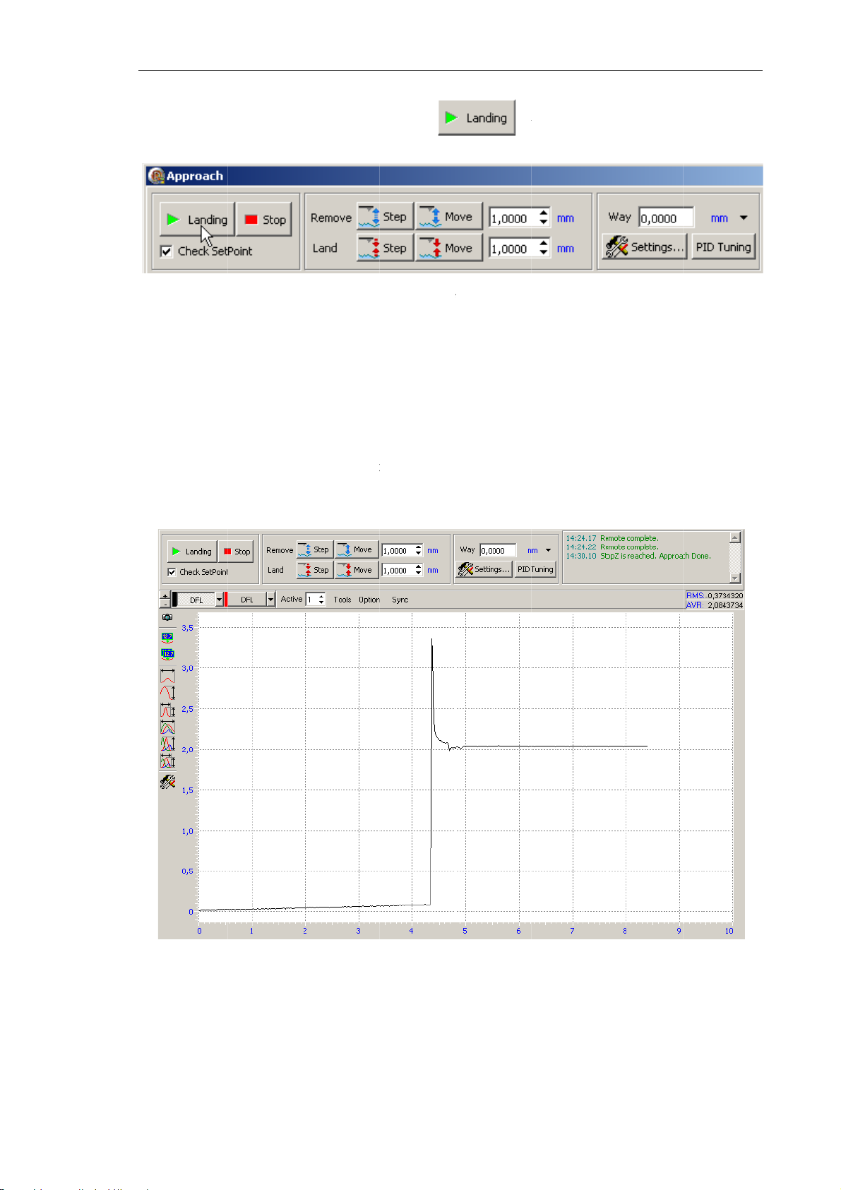
5.
scoPrab
A
h
a
e
3
p
s
F
p
a
w
n
o
s
t
g
f
b
r
r
o
C
bu
A
a
c
s
s
e
e
s
t
p
i
e
p
h
o
s
9
e
e
e
n
Start the
pproac
approach
window (
rocedure
ee Fig. 7-5
ith the
).
hapter 7. P
tton in th
rforming M
Control
asurement
anel of th
D
uring the
o
cilloscope
mpletes.
oviding th
out 10 to
pproach
and state
approach
0 seconds
ig. 7-5. Co
rocedure,
of the sc
parameter
nd the sys
trol panel o
serve va
anner exte
are set co
em goes to
the
ppro
iations of
nsion indi
rectly, the
following
ch
window
the
DFL
ator. Wai
approach
tate (see F
ignal in t
until the
rocedure c
g. 7-6):
e softwar
procedur
mpletes i
Fi
. 7-6. Appr
ach proces
5
Page 68
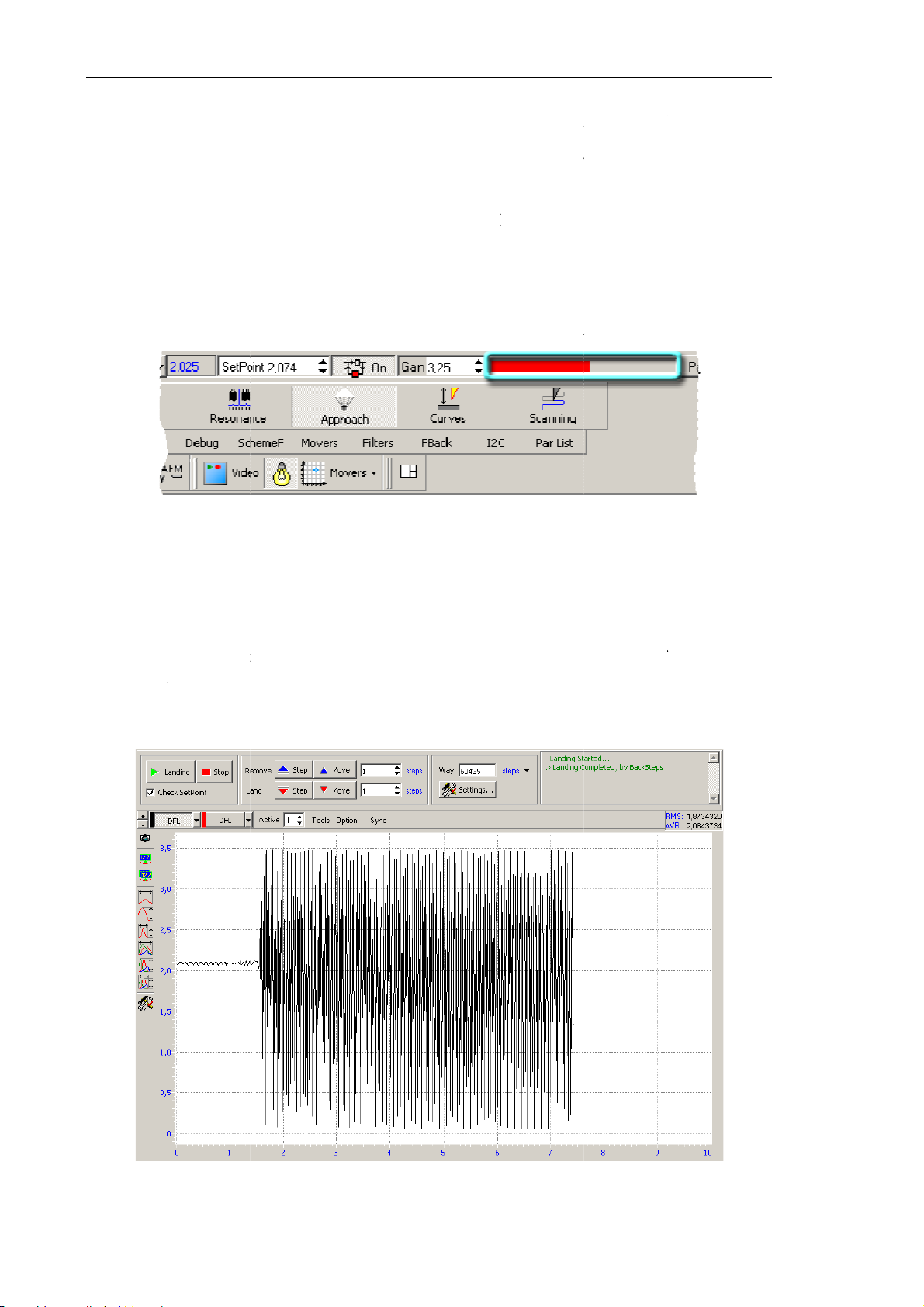
Solver NE
X
i
o
g
e
e
h
e
g
u
n
n
r
c
o
i
S
n
r
l
t
r
n
n
u
t
h
n
i
e
p
d
e
F
r
k
u
c
e
N
e
w
e
w
r
v
k
v
r
.
a
D
q
p
i
e
a
t
e
m
s
u
t
a
a
t
g
e
F
p
fe
e
n
r
c
e
n
r
l
o
t
.
a
a
m
i
●
The si
mainta
that th
range;
●
The s
DFL
●
The m
●
The st
●
Lengt
T SPM. Inst
gnal
ins the Z-s
s position
ftware osc
si
nal to the
ssage “
pper moto
of the indi
DFL
La
uction Man
increases
anner in t
f the scan
lloscope d
et Point
ding Com
is disable
cator bar d
al
o the lev
e position
er is appro
splays the
l
vel;
leted
” app
;
creases do
l of
Set P
here the
ximately e
DFL(t)
gra
ars at the r
n to some
oint
para
FL
value i
ual to half
h that ill
ght top of
intermedi
eter, the
equal to
of the sca
strates inc
he Approa
te value (s
edback lo
S
t Point
ner extensi
easing of
h window.
e Fig. 7-7)
. N
op
te
on
he
7.1.1.4.
The great
processin
gain (let
unstable a
a significa
Adjus
r is the
speed in
s call it th
d noise ge
t alternati
ting Wo
evel of th
he feedbac
eshold val
eration oc
g compon
ig. 7-7. App
king Le
e feedbac
loop. Ne
e), the mo
urs. Unde
nt (see Fig
oach compl
el of th
gain (
ertheless,
de of oper
this condi
7-8).
Ga
eted
Feedb
in
parame
at some hi
tion of th
ion, the
D
ck Gai
er), the g
h level of
feedback
L
signal is
eater is d
the feedb
oop beco
supplied w
ta
ck
es
th
Fig. 7-8.
60
oise gener
tion in the f
edback loo
Page 69
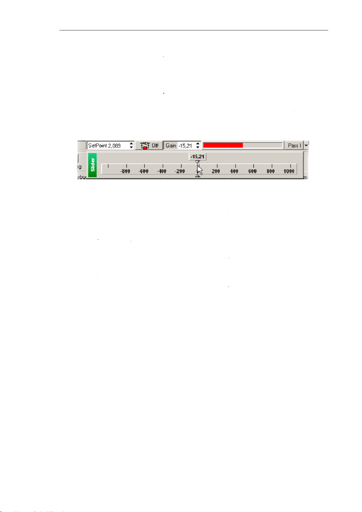
F
oth
o
p
l
e
e
c
y
o
Th
n
b
g
n
u
i
t
e
a
i
v
e
e
F
o
a
e
e
f
l
s
u
n
e
G
s
s
p
o
a
)
d
i
e
d
C
e
m
h
m
c
r
o
e
n
g
i
T
e
h
e
5
u
n
o
a
s
e
e
f
e
e
g
be
r stable o
reshold va
G
ain
input fi
T
adjust th
1.
Double-
the feedb
eration, it
ue where
ld.
working l
lick the
G
ack gain w
s recomm
he noise g
vel of the
in
input fie
ll appear (
nded to de
neration
eedback g
d in the M
ee Fig. 7-9
fine the fe
ccurs. The
in, perfor
ain Parame
.
hapter 7. P
dback gai
feedback
the follow
ters panel.
rforming M
to less 0.
ain is adj
ng steps:
he adjusti
asurement
÷0.7 of th
sted in th
g slider o
2.
Graduall
oscillosc
NOTE.
3.
Determi
eginnin
compone
4.
Decrease
used in f
decrease
pe.
e
Gain
le
e the valu
of the g
t in the D
the value
rther oper
Fig. 7-9. Adj
the
Gai
el should b
of the
neration i
L signal (
f the
Gain
tion.
sting slider
level an
negative
ain
param
identifie
ee Fig. 7-8
arameter t
of the
Gain
watch t
n contact
ter at whi
by appea
).
0.5÷0.7
parameter
e
DFL
l
odes.
h noise g
ance of a
f the thres
vel in th
eneration
noticeable
old. This v
e softwar
ccurs. Th
alternatin
lue will
61
Page 70
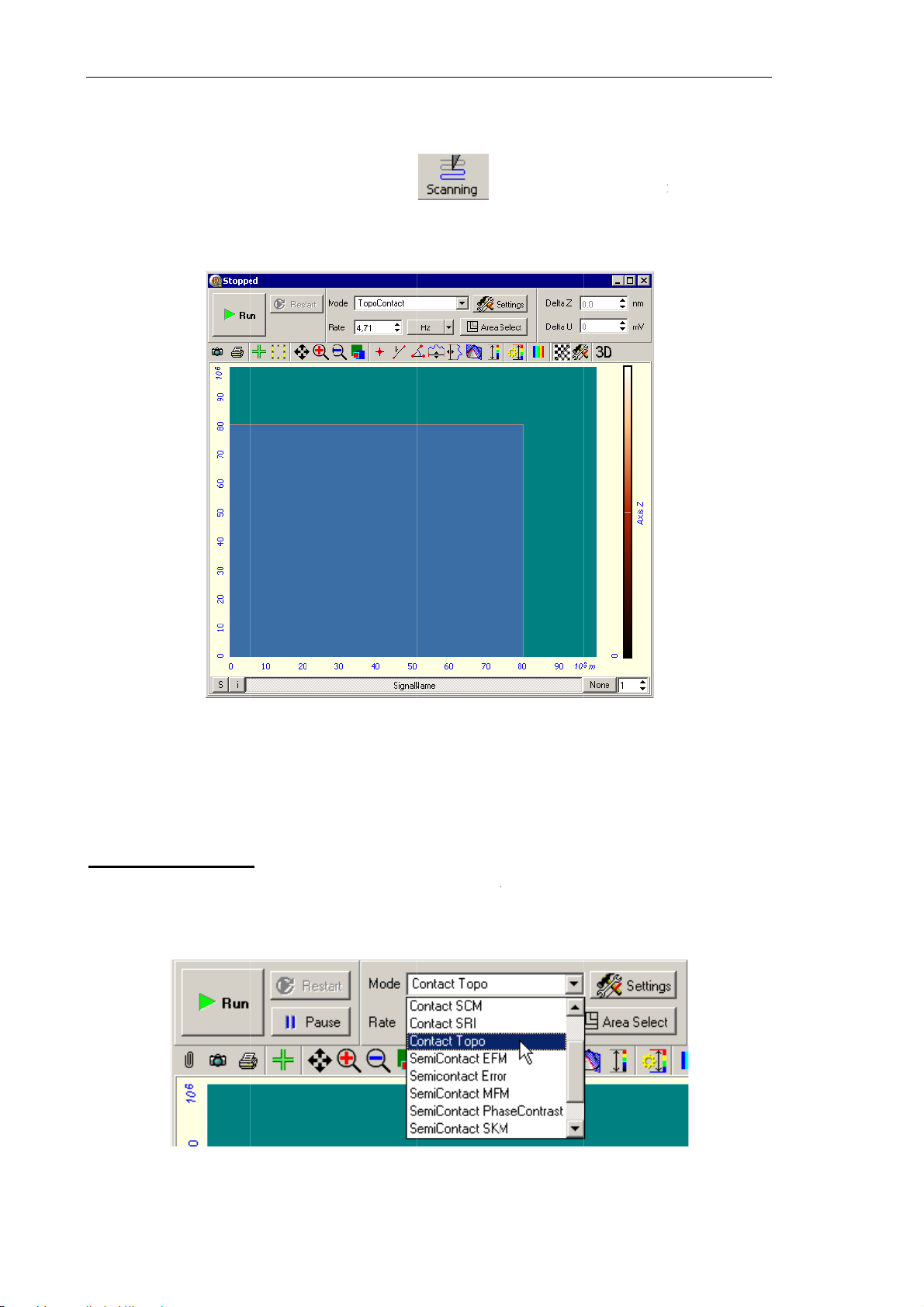
Solver NE
X
S
a
m
o
A
s
r
S
i
e
o
1
r
u
l
w
F
a
r
a
n
c
w
d
a
h
r
b
n
d
l
t
p
e
r
p
e
r
n
a
e
e
d
i
T SPM. Inst
uction Man
al
7.1.1.5.
Open the
The top p
(see Fig. 7
Adjus
canning
rt of the
-10).
ting Sca
w
indow by c
canning
nning P
icking the
indow co
ramete
tains a pa
s
utton in th
el to cont
Main Ope
ol the sca
ations pan
ning proc
l.
ss
The botto
investigati
Selecting
Select the
window (
sequences
of the w
n.
FM mod
Contact T
ee Fig. 7-
in the cont
ndow cont
po
mode
1). This
oller.
ig. 7-10.
ins a Vie
in the
Mo
esults in
S
anning
er to disp
e
list of
utomatic
win
ow
ay topogra
he Contro
erforming
hy of the
l panel of
all necess
surface un
the scanni
ry switch
er
ng
ng
Fig. 7-11
62
. Selecting t
e Constant
Force Mod
Page 71
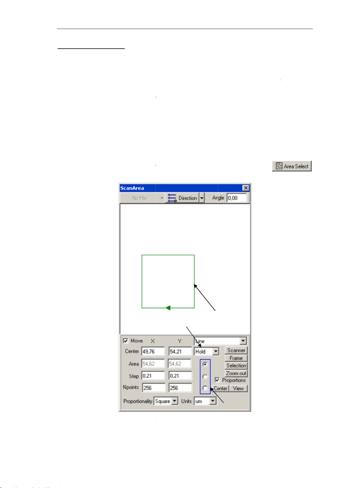
S
e
ore
o
e
m
m
r
t
e
a
r
i
d
b
n
e
a
l
c
fa
n
s
w
h
2
n
o
h
s
o
S
e
e
g
a
k
C
r
b
n
d
B
2
w
t
1
e
d
h
s
r
e
i
e
e
s
3
g
e
t
g
e
lecting th
T
choose
commenda
●
If height
maximu
scan are
prelimina
tions:
difference
scan fiel
y dimensi
n the surfa
is recomm
ons of t
e profile i
ended;
e scan a
known to
hapter 7. P
ea, regar
e within t
rforming M
for the
e Z-scann
asurement
followin
r range, th
If height
●
10÷15 μ
paramete
enlarged.
T
select or
1.
Open th
button in
difference
) should
s, includi
o resize th
Scan are
the Contro
in the sur
e prelimi
g speed of
scan area,
selection
panel of t
ce profile
arily expl
canning,
perform th
indow (s
e
Scannin
is unknow
red for fin
et Point, F
following
e Fig. 7-1
window.
, a small
ing prope
Gain
. Th
steps:
) by click
ized scan
levels of
n the scan
ng the
area (abou
controllin
area can b
3
2
Fig. 7-1
1 – sca
3 – l
. Scan are
area; 2 – p
cking/unloc
selection
arameter se
ing parame
indow
lector;
ers
6
Page 72
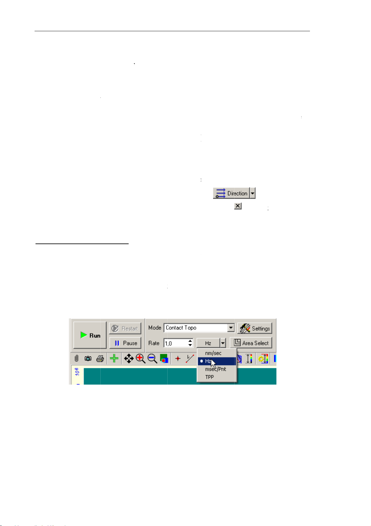
Solver NE
X
d
n
n
l
a
d
c
b
e
g
t
t
t
w
v
s
u
n
R
v
r
.
a
a
e
e
m
n
e
r
e
i
e
n
w
e
u
o
e
f
n
p
i
w
Area
a
s
h
n
o
b
n
u
2
o
e
i
c
d
o
o
w
b
e
o
h
t
n
g
e
m
e
o
n
i
a
u
)
s
m
t
a
e
e
y
n
Area
a
h
e
e
s
t
n
m
e
i
d
o
2
r
c
r
w
t
g
i
h
i
d
w
d
t
u
e
t
t
e
t
r
h
a
T SPM. Inst
uction Man
al
2. In the
Hold
a
vary u
a.
Ho
mo
difications.
sec
ond free p
b.
Ch
un
3. Select
modifi
4. Adjust
etwe
rectan
5. Move
6. Select
7. Close
windo
rop-down
Change
der modifi
d
selected:
nge
select
er modific
the param
ation mod
the para
n scan poi
le (pos. 1).
he scan ar
he scan di
he Scan ar
.
list (see p
This mod
cations as
the param
Adjustme
rameter to
ed: the
tion of the
ter that w
, pos. 3)
eters
ts, and tot
a to the de
ection in t
a selectio
s. 3 on Fig
s define h
ollows:
eter mark
ts of any
rovide the
parameter
two others
ll be fixed
ith the sele
,
Step
l of scan p
ired locati
e drop-do
window
. 7-12), sel
w the para
d with th
of the tw
r correspo
marked w
proportion
an
n with the
n menu of
y clicking
or linked
tor (pos. 2
NPoints
ints. The
ct betwee
eters
selector
other par
dence wit
th the sel
lly to valu
nder adju
.
o define
can area is
ouse.
the
he button
the modif
,
Step,
an
(pos. 2) is
meters wi
the fixed
ctor (pos.
of the thi
tment (ac
he scan a
displayed
but
at the ri
cation mo
NPoints
fixed un
ll change
ne.
) will adj
d paramet
ording to
ea size, s
ith the gr
on.
ht top of
es
ill
er
he
st
.
he
ep
en
he
Adjusting
Optimal
dimension
that with
Low scan
properties
1. In the
the scann
alue of th
and exter
neven topo
ing speed
are unkno
ate
list, s
ng speed
scanning
al conditi
graphy and
(defined
n. To defi
lect Hz as
speed dep
ns. A smo
large heig
y the
e the
Ra
Rate
nits of sca
Fi
nds on s
th surface
t differenc
e
paramet
parameter,
frequenc
. 7-13
mple surfa
can be sca
.
r) is reco
perform th
(see Fig. 7
ce propert
ned at hig
mended
following
-13).
es, scan a
er speed t
f the surf
styeps:
ea
an
ce
2. Enter
alue in the
range 1.5÷
Hz in the
Rate
input
field.
64
Page 73
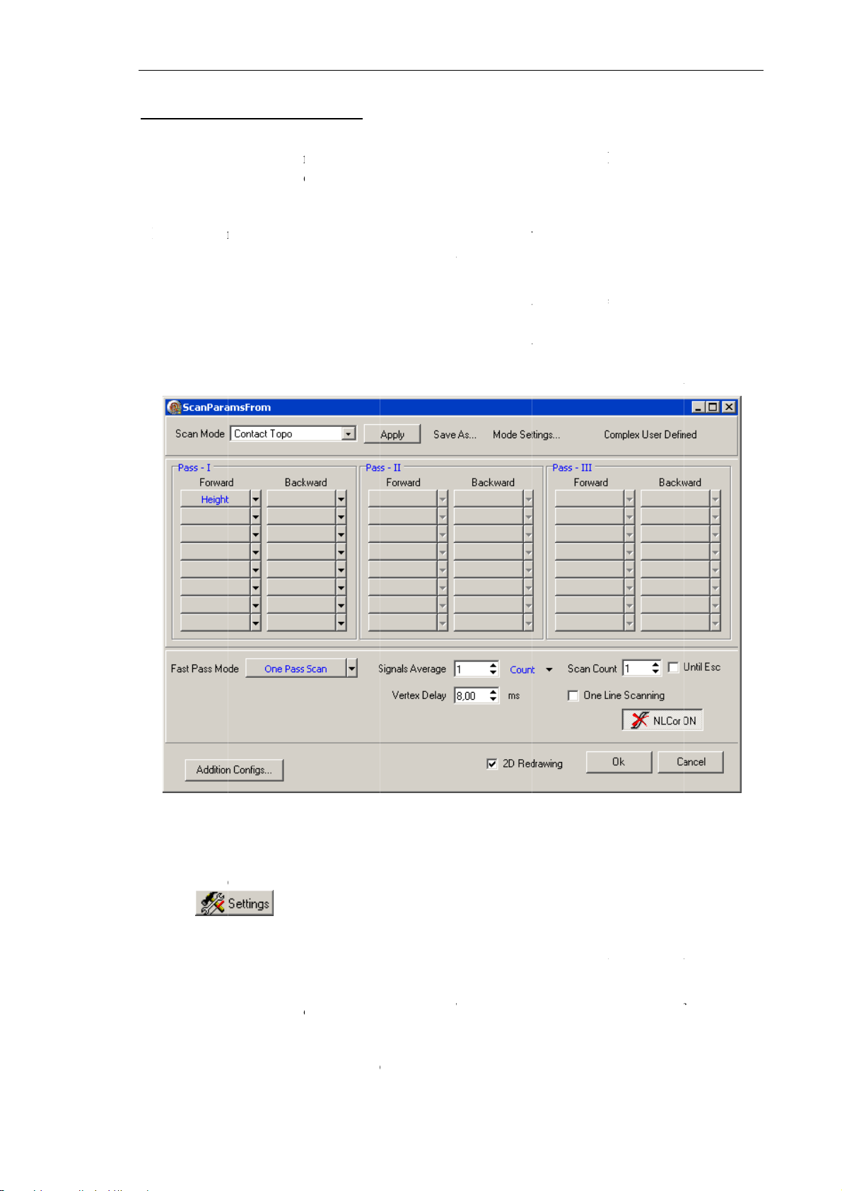
S
w
hausuPr
HthinTh(s
a
o
iTo
h
n
y
h
e
m
c
e
u
i
h
e
f
t
n
a
m
d
s
e
m
g
A
y
k
t
a
t
e
s
e
a
b
t
b
s
s
n
.
m
c
e
o
m
c
a
C
e
h
t
d
e
t
u
u
a
e
i
e
m
n
i
d
a
C
e
n
D
r
p
e
a
d
m
p
h
e
w
(
S
n
e
e
e
g
h
f
o
e
t
n
d
m
w
h
e
e
r
v
i
e
n
k
r
n
b
h
e
h
fr
s
5
d
s
e
s
w
,
e
g
g
n
n
t
itching t
T
e measuri
tomaticall
pplied wit
e detectio
g modes
after the
correspon
signals
re associa
ode has
ing signal
ed with is
een select
by defaul
standard d
d. For ma
.
hapter 7. P
tection si
y-pass tec
rforming M
nals that a
niques, e
asurement
e assigne
ery pass i
ofile of th
owever, so
e default li
every dire
e list of d
ee Fig. 7-1
P
ss II
, and
F
rward
d
rection wh
detection
st of detect
tion of sa
tection si
4). Signals
Pass III
col
mn displa
le the
etimes d
.
Bac
ignal is di
tection of
ion signals
ple move
nals is ava
of a parti
pass pan
s signals t
ward
colu
played in a
on-default
The instr
ent during
ilable thro
ular pass
l contains
detect wh
n enlists s
separate 2
signals is
ment is ca
measurem
gh the Sc
re arrange
two colu
n the sam
gnals for t
Viewer o
equired. F
able to rec
nts.
n paramet
in separa
ns,
Forwar
le moves i
e backwar
Scanning
r this, you
ord up to e
rs adjustm
e table pa
d
and
Bac
the forwa
moveme
window.
can chang
ght signal
nt windo
els
Pass I
ward
. Th
d scannin
t.
modify t
1.
Open th
the
signals o
2.
Select th
e list of de
Scan p
but
the select
e desired
Fig. 7-14. S
ection sign
rameters
on in the
d mode ar
ignals in t
an paramet
als, perfor
djustment
ontrol pa
displayed
e drop-do
rs adjustm
the follo
window
el of the
n correspo
wn lists to
nt window
ing steps:
ScanPara
canning
ding cells
change t
sFrom
)
indow. T
of the tabl
e set of t
y clickin
e detectio
s.
e detectio
signals.
NOTE. A
of the de
3.
Click the
signal nec
ection sign
OK
utton
ssary for
ls.
to save mo
he selecte
ifications
scan mod
nd to clos
can not b
the dialog
removed
.
om the lis
6
Page 74
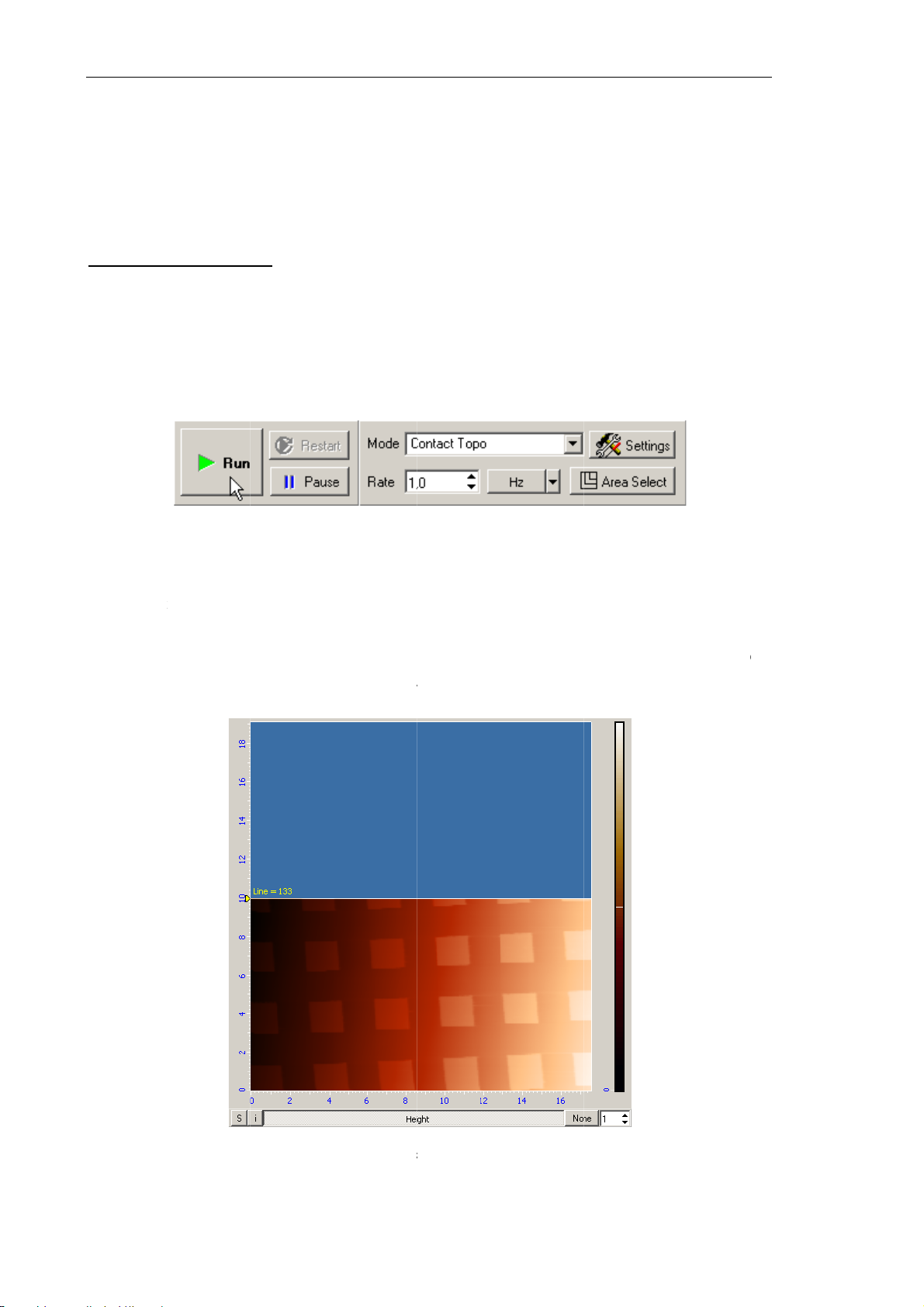
Solver NE
X
g
m
o
l
s
c
t
by
r
a
r
n
n
Q
n
p
o
l
n
f
u
w
e
h
C
v
g
a
h
n
e
s
r
g
c
t
n
r
a
e
y
d
o
r
g
n
o
d
n
g
r
o
t
p
T SPM. Inst
uction Man
al
7.1.1.6.
Hereafter,
(standard
Starting
Scanning
(the samp
parameter
To start s
(see Fig. 7
Scan
the scanni
rating TG
easureme
f the sam
e has appr
have been
anning, cl
-15).
ing
g process
-1, 3 μm r
ts
le surface
ached to t
set).
ick the
Fig. 7-15.
Ru
ill be expl
solution).
should be
e probe, t
n
button i
ontrol pan
ined with
preceded b
e operatio
the Cont
l of the
Sca
he exampl
y necessar
point is a
ol panel o
nning
wind
of a recta
preparati
justed, an
f the
Sca
w
gular grati
n procedu
all scanni
ning
wind
ng
es
ng
w
This resul
●
Linescan a
this is
s in the fol
-line scan
ea appears
n image o
owing acti
ing of the
in the 2D
the rectan
ity of the
sample su
Viewer of
ular gratin
ystem:
face starts
the scan d
;
and the co
ta (see Fi
respondin
. 7-16). In
image of
our exam
he
le,
Fig.
7-16. Surfa
66
e topograph
y image
Page 75
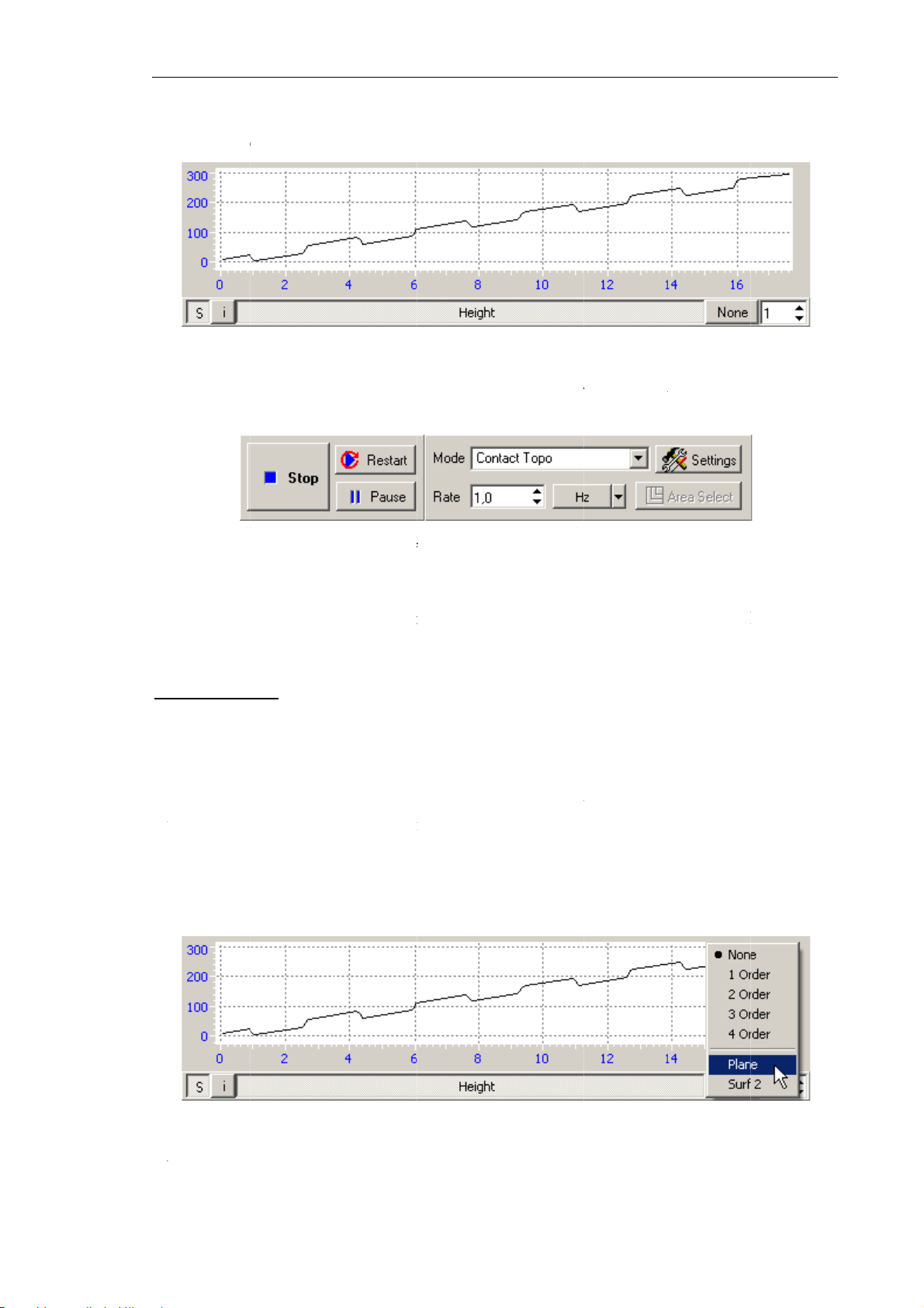
●
h
e
r
w
o
o
m
Ndi
e
t
c
t
x
d
n
i
h
a
b
h
n
o
o
e
s
u
F
o
t
e
F
n
f
n
t
h
n
T
d
g
p
e
p
m
7
e
e
C
r
m
g
n
t
a
l
t
F
d
n
n
n
e
a
bu
e
o
m
o
e
n
2
u
u
e
p
g
g
E
t
e
t
e
s
7
e
p
e
n
g
e
l
e
If the S
1D View
utton in t
r will disp
e left bot
lay the det
om of the
ction signa
2D Viewe
l in real ti
hapter 7. P
of the sc
e (see Fig.
rforming M
n data is
7-17);
asurement
ressed, th
●
The
(see Fig.
S
ould the s
T
ilt subtrac
D
ata in the e
d
gree in X
C
ontribution
p
ocess with
indow. By
Res
art
7-18).
Fi
g. 7-18. Co
anning pr
ion
irection.
of the tilt t
default, thi
button
ample ab
proper sel
becomes e
trol panel o
cedure be i
ve (see Fig
o the detec
ction of t
button is i
ig. 7-17.
H
abled and
the
Scanni
terrupted,
. 7-16, Fig.
ed landsca
e
Subtract
the
None
ight
signal
caption of
n
window i
click the
7-17) reve
e can be e
control at
state (see
the
the cours
S
op
button
l that the s
iminated i
he right b
ig. 7-17).
Run
tton chan
of scannin
r use the <
ample is til
mediately
ttom of th
es to
Sto
sc> key.
ed to som
in the sca
Scannin
T
activate
c
rrespondi
i
age (see F
OTE. In t
rection to
run-time s
g list (see
g. 7-16) is
e process
pply the c
btraction,
ig. 7-19).
transforme
of definin
rrection a
click this
his entails
into the i
Fig.
the corr
pears to th
button an
subtractio
age show
-19
ction tech
left of the
select th
of the pla
in Fig. 7-
ique, a b
Subtract
Plane
e tilt, and
0.
tton for s
b
tton.
op
tion in th
he origina
lecting th
6
Page 76
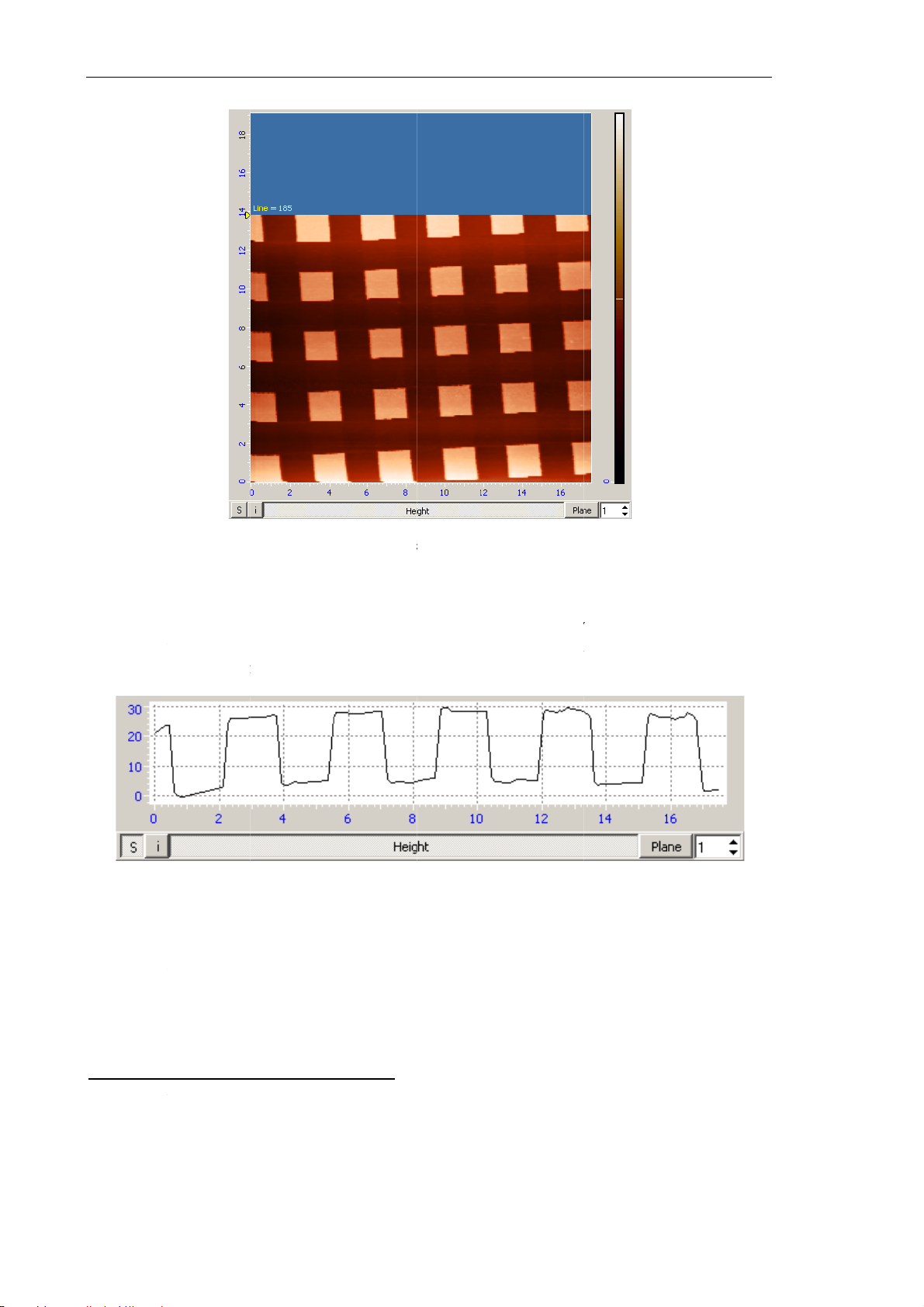
Solver NE
X
c
r
w
o
ac
a
g
w
r
d
n
m
i
e
i
u
e
o
7
f
h
h
c
e
o
m
n
a
e
c
c
a
o
n
e
a
w
l
c
h
i
m
pe
r
g
t
T SPM. Inst
uction Man
al
With the
signal co
(compare
orrection
rected for
ith the sig
Fig.
efined, th
the tilt c
al in Fig.
7-20. Surfa
1D View
ntribution.
-17).
Fig. 7-21.
e topograph
r of the s
The resul
Height
sign
y image
an data
ting signa
l
ill display
is shown
the detecti
in Fig. 7-
on
21
NOTE. C
the
Subtr
llected fra
option.
es miss in
ormation
n correcti
ns of the s
an data
rformed w
ith
Tuning p
Quality of
frequency,
feedback
scanning
68
rameters
the acquir
Rate
ain,
Gain
ith visual
(see
.
n the scan
surface i
Fig. 7-22)
Either of t
nspection
process
age esse
, the oper
ese param
ow modifi
tially depe
ting point,
ters can b
ations imp
ds on suc
Set Point
adjusted
ct on the i
paramete
(see Fig. 7
nstantly in
age bein
s as scanni
-23), and
the course
collected.
ng
he
of
Page 77
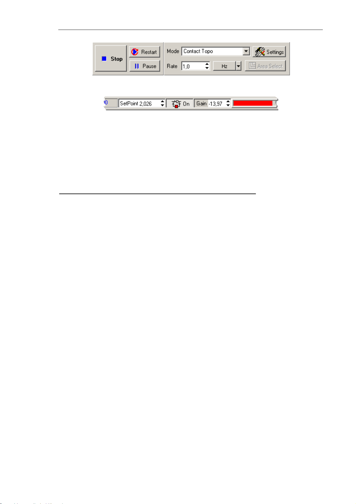
Fig. 7-22
Fig. 7-23
The Restart button serves to restart scanning again.
Chapter 7. Performing Measurements
NOTE. Scanning is recommended to restart (using the
Restart
button) after any of
scanning parameters is changed.
Some recommendations on optimization of scanning parameters
The choice of the optimal value of scanning speed depends on properties of the sample, on
dimensions of the scan area, and on external conditions.
Smooth surfaces can be scanned at a speed higher than those with sharp features and steep
slopes.
It is recommended to start scanning at a lower scanning speed, increasing it gradually until
distortions affect the landscape profile.
Scanning speed should be reduced when surface features in the scan direction are not
detected.
In measurements of soft materials, the images may be affected by “dragging effects”
caused by surface features in the scan direction. In the event of such effects, it is
recommended to reduce the scanning speed as well as to increase the Set Point level in
order to lower pressure on the sample.
69
Page 78
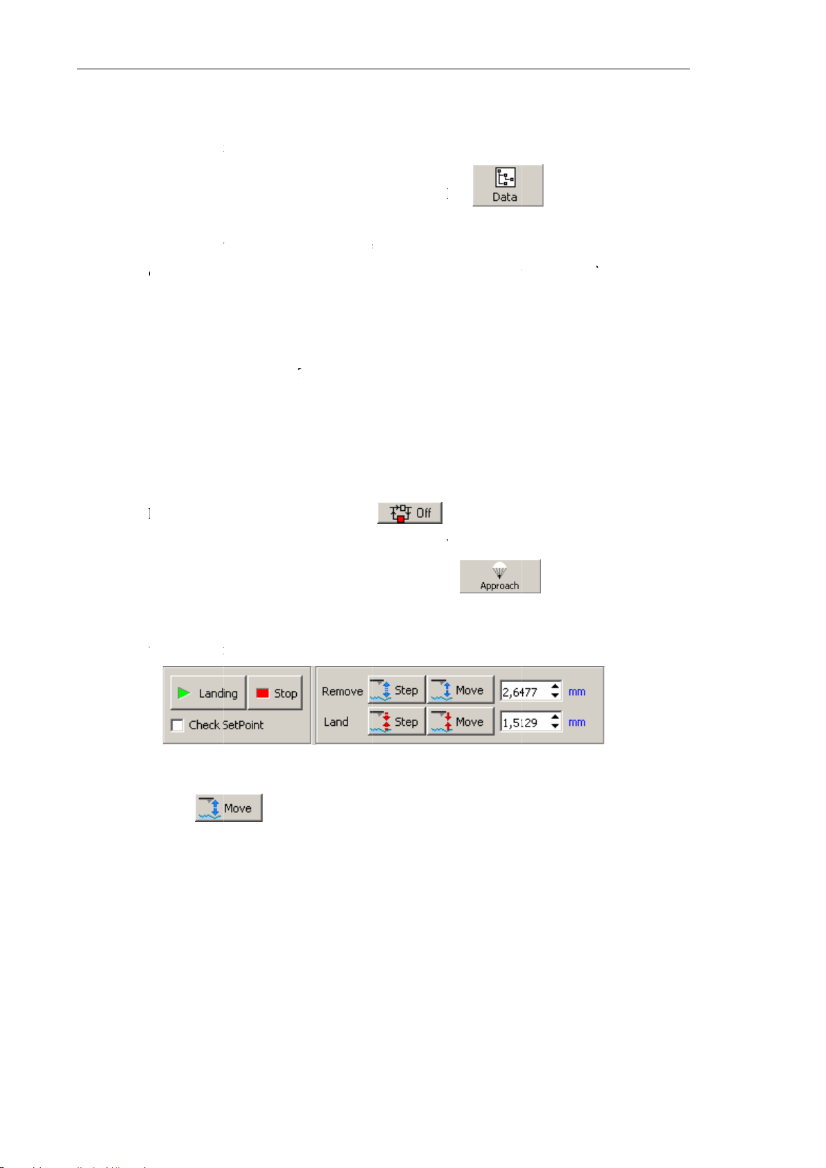
Solver NE
X
e
t
o
g
n
a
e
h
t
u
r
g
t
v
l
N
e
a
”
p
n
k
e
App
n
v
n
u
u
e
w
e
C
N
i
X
M
t
e
p
n
e
b
o
D
e
f
e
i
m
n
g
C
i
g
t
h
h
n
t
r
b
w
e
n
e
g
m
t
a
A
p
ys
f
w
a
m
a
t
T SPM. Inst
uction Man
al
7.1.1.7.
To save m
1. Open
Operat
2. Select
3. A dial
C:\Pro
4. Type i
NOTE.
“NoN
7.1.1.8.
To compl
Savin
asuremen
he
Image
ions panel.
File
→
Sa
g box wi
ram Files\
a filenam
By def
meXX.mdt
Com
te operatio
Meas
data on th
Analysis
e All Fram
l appear.
T-MDT\
and save
ult, the
where X
leting
, perform
rement
hard drive
indow by
s
Main m
hoose a
ova_9).
t with the
acquired
is the file
easure
he followi
ata
, perform t
clicking t
nu comma
older to s
xtension *.
images a
ndex in the
ents
g steps:
e followin
e
of the
I
ore the da
mdt.
e stored
folder Nov
steps:
button
age Anal
a (the de
in files
_9.
in the M
is
window.
ault folder
with na
in
is
es
1. Open t
2. Retrac
a. Op
Op
b. In
val
c. Cli
e feedbac
the sampl
en the
erations pa
the
Remo
e in the ra
ck the
loop by r
from the
roach
wi
el.
e
input fi
ge of 2÷3
utt
leasing the
robe throu
dow by c
ld in the
mm (see F
Fi
n to retrac
h the follo
licking th
ontrol pa
g. 7-24).
. 7-24
the sampl
utton.
ing steps:
el of the
from the
button
pproach
robe.
in the M
indow, en
in
er
70
Page 79
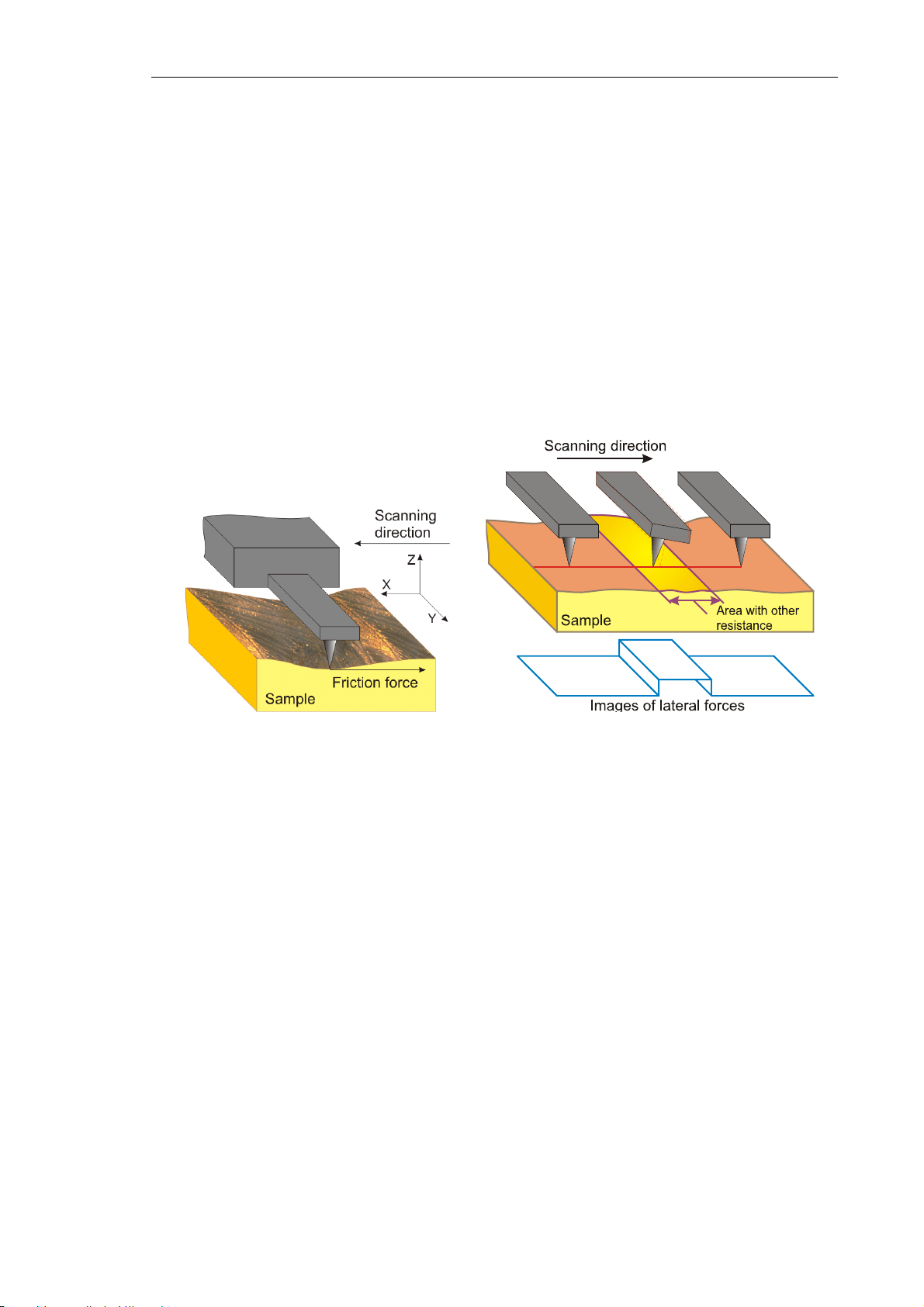
Chapter 7. Performing Measurements
7.1.2. Lateral Force Microscopy
7.1.2.1. Brief Description
The Lateral Force Microscopy facilitates discrimination between areas with different
coefficients of friction as well as reveals specific features of surface topography. This
mode is useful in research of semiconductors, polymers, film coatings, memory media for
physico-chemical properties of the surface (in particular, deterioration), tribology
characteristics etc.
The Lateral Force Microscopy is based on the following physical ground. While scanning
in this mode, a torsion deflection of the probe occurs in the direction perpendicular to the
longitudinal axis of the cantilever additionally to the normal deflection (see Fig. 7-25). It is
caused by moment of the force acting on the tip of the probe.
Fig. 7-25 Fig. 7-26
At small deflections, the twist angle of the probe is proportional to the lateral force. The
magnitude of the twist is measured with the optical detection system of the instrument.
This detection system generates the
LF signal whose variation is proportional to the value
of the torsion deflection of the cantilever. This signal provides imaging of the local friction
along the sample surface.
The twist angle of the probe varies when the probe moves along a flat surface with regions
that differ in their friction coefficients (see Fig. 7-26). This variation provides information
on distribution of local friction properties. Unfortunately, such interpretation becomes
invalid if the landscape is not flat.
Nevertheless, this technique offers good imaging of surface features in small scales. For
example, lateral forces data provided easy determination of the atomic lattice parameters of
mica and other lamellar materials.
71
Page 80
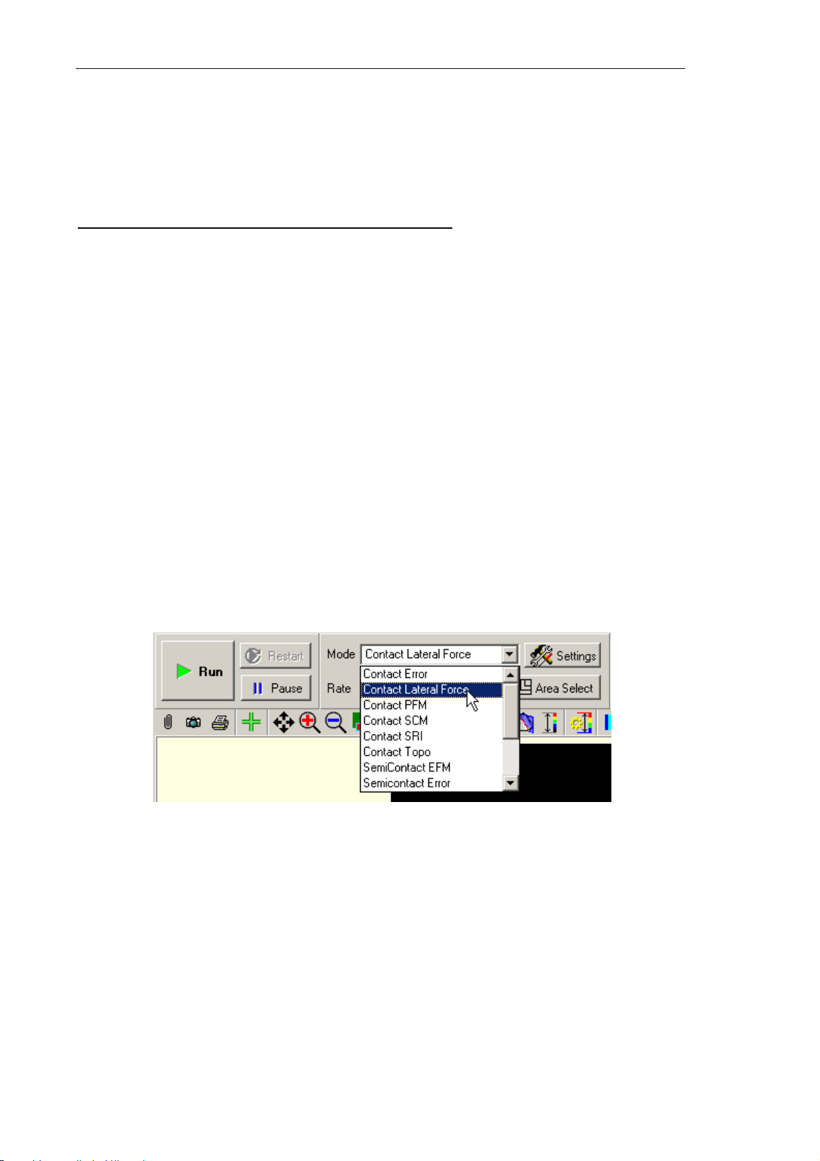
Solver NEXT SPM. Instruction Manual
7.1.2.2. Procedural Sequence
Procedures of the Lateral Force Mode are based on those of the Constant Force Mode that
is described in detail in sect. 7.1.1 “Constant Force Mode” on p. 55.
Main procedures involved in the Lateral Force Mode
1. Adjusting the Controller Configuration (see i. 7.1.1.1 on p. 56).
2. Adjusting Initial Level of the DFL Signal (see i. 7.1.1.1 on p. 56).
3. Approaching the Sample to the Probe (see i. 7.1.1.2 on p. 56).
4. Adjusting Working Level of the Feedback Gain (see i. 7.1.1.3 on p. 58).
5. Adjusting Scanning Parameters (see i. 7.1.1.4 on p. 60).
6. Scanning (see i. 7.1.1.5 on p. 62).
7. Saving Measurement Data (see i 7.1.1.6 on p. 66).
8. Completing Measurements (see i 7.1.1.7 on p. 70).
7.1.2.3. Scanning
The basic difference of operation in this mode from that of the Constant Force Mode is in
the step of item. 7.1.1.5 “Scanning” on p. 62 (see sect. “Selecting AFM mode” on p. 62)
where the Contact Lateral Force option in the Mode list should be selected instead of
Contact Topo (see Fig. 7-27). This selection provides proper automatic electronic
arrangement required by the mode.
Fig. 7-27. Selecting the Lateral Force Microscopy
To start scanning, click the Run button in the Control panel of the Scanning window.
This launches line-by-line scanning of the sample surface and the 2D Viewer of the scan
data will display three 2D data views. The first view shows the surface landscape (Height
signal) while the other two display distributions of the lateral force (LF signal)
(see Fig. 7-28) detected in forward and backward sweeps of the scan lines.
72
Page 81
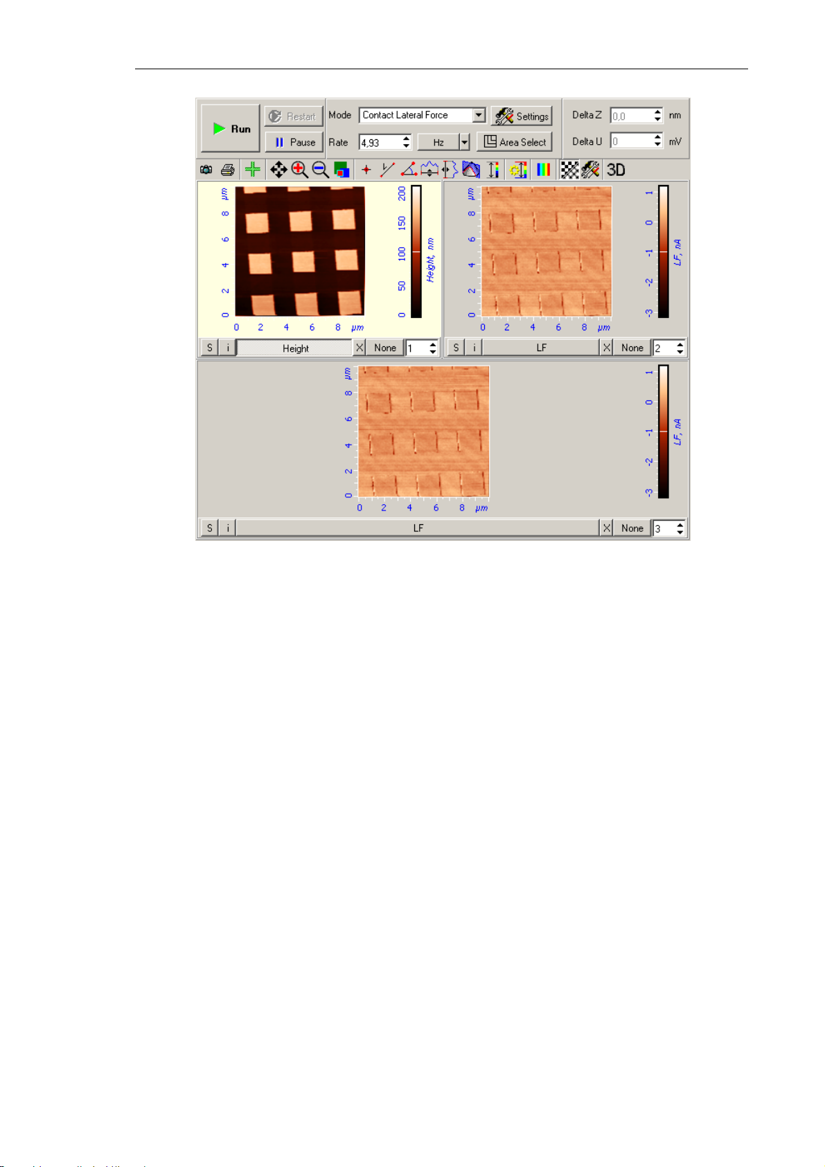
Chapter 7. Performing Measurements
Fig. 7-28. Images of surface topography and distribution of lateral forces
7.1.3. Spreading Resistance Imaging
7.1.3.1. Brief Description
The Spreading Resistance Imaging mode is a very efficient AFM mode. It is employed in
various fields, including defects in conductive and low conductive films, materials
characterization in terms of local resistance etc. This mode uses a conductive probe that
comes in contact with the sample surface. The probe is applied to a bias voltage. The
resulting current through the sample is measured as a function of the probe position
simultaneously with surface topography acquisition. The latter uses the Constant Force
mode. It is easy to prove that, under the assumption of constancy of contact probe-surface
resistance for a given bias voltage, the detected current is proportional to local resistance of
the sample.
Among typical applications of the mode are finding actual geometrical dimensions of
source-drain regions in MIS transistors, localization of p-n junctions, study of dopants
distribution in semiconductors etc.
73
Page 82
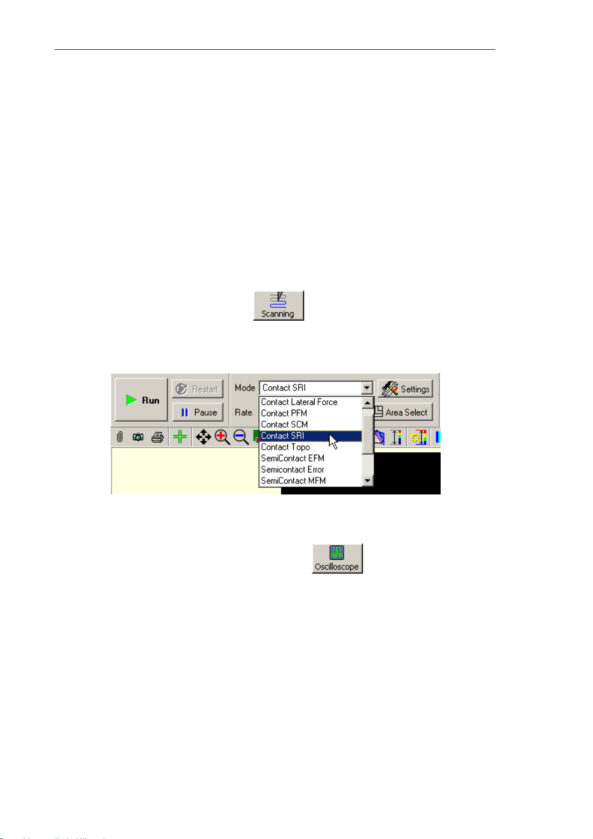
Solver NEXT SPM. Instruction Manual
7.1.3.2. Procedural Sequence
Procedures of the Spreading Resistance Imaging Mode are based on those of the Constant
Force Mode that is described in detail in sect. 7.1.1 “Constant Force Mode” on p. 55.
Before starting the Spreading Resistance Imaging, make preparations for measurements
and perform measurements of surface topography by the Constant Force Mode
Remember to use the measuring head equipped with the conducting contact probe.
After preliminary measurements of surface topography by the Constant Force Mode, adjust
parameters for operating in the Spreading Resistance Imaging Mode.
7.1.3.3. Adjusting Scanning Parameters
1. Open the Scanning window with the button in the Main Operations panel.
2. Select the Contact SRI mode in the Mode list on the Control panel of the scanning
window (see Fig. 7-29). This causes automatic rearrangement of the instrument to
provide the desired mode.
Fig. 7-29. Selecting the Spreading Resistance Imaging Mode
3. Open the software oscilloscope window with the button.
4. In the Oscilloscope window, select displaying of the
IprAFM signal (see Fig. 7-30).
74
Page 83
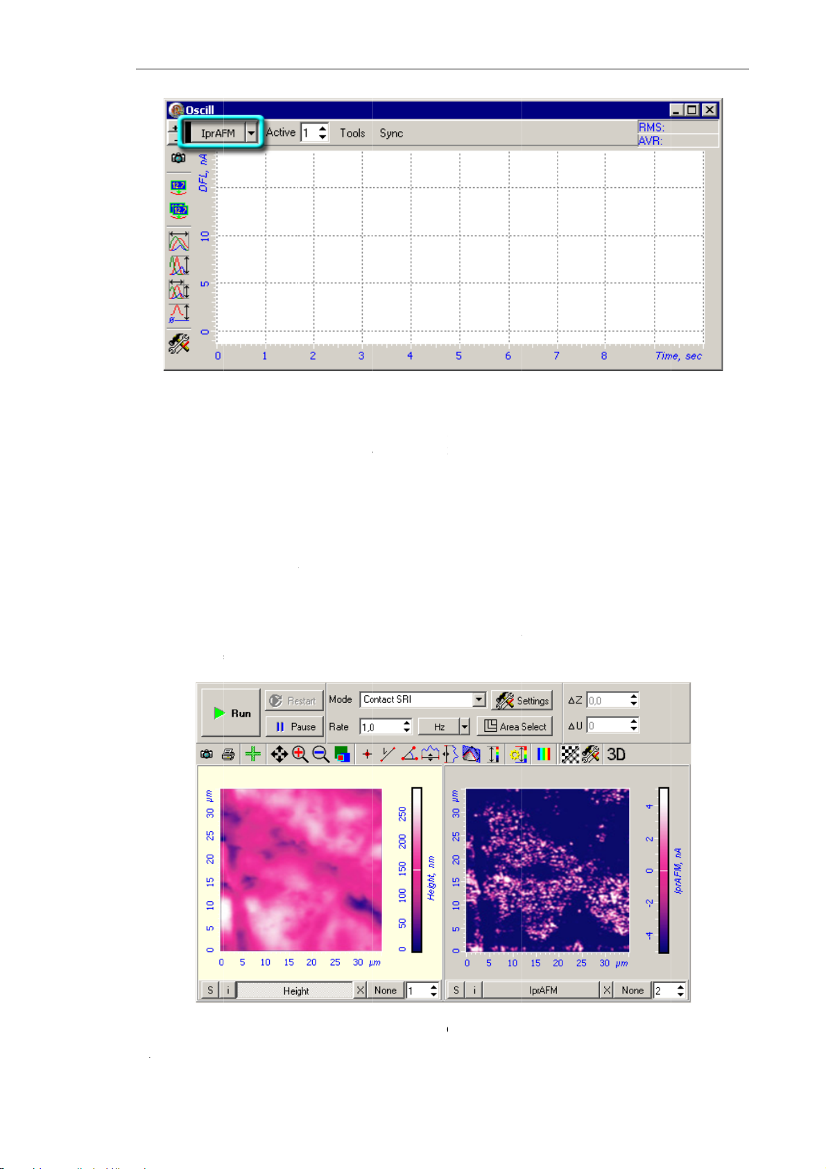
7
cThda
N
e
o
t
e
p
e
h
S
m
A
e
n
n
i
D
d
e
e
o
B
o
g
w
y
e
g
g
h
t
t
m
s
i
d
C
O
n
c
w
p
o
o
hapter 7. P
e
e
h
M
2
f
u
d
e
o
h
e
a
F
s
5
n
m
f
n
t
rforming M
asurement
5.
Enter th
program
oscillosc
.1.3.4.
C
lick the bu
s
anning.
is launch
ta will dis
si
gnal) whil
Fig. 7-30.
probe-sa
window.
pe is in th
Scanni
ton
Run
s line-by-l
lay two 2
the secon
electing th
ple bias v
djust the
range 1÷1
g
i
the Contr
ne scannin
data vie
one displa
IprAFM
ltage in t
V
bias vol
0 nA.
l panel of
of the sa
s. The fir
s distribut
si
nal in the
e BV input
age so that
he
Scanni
ple surfa
t view sho
on of the s
scilloscop
field of t
the
IprAF
window
e and the
s the sur
reading c
window
e top bar
level in t
to start th
D Viewer
ace landsc
rrent (
IprA
f the Mai
e progra
process o
of the sca
pe (
Heigh
M
signal).
Fig. 7-31
OTE. Brig
tness in th
. Landscap
IprAFM
image and
si
nal image
istribution
is proporti
f spreading
nal to con
current
uctivity.
7
Page 84

Solver NEXT SPM. Instruction Manual
How to Improve Image Quality
ATTENTION! Too tight mechanical contact between the probe and the
sample may cause damage to the conductive coating of the probe.
If necessary, you can try the following recommendations:
● Adjust the SetPoint parameter (it controls pressure applied to the sample by the probe);
● Adjust the bias voltage applied between the probe and the sample (Bias Voltage
parameter). Note that excessive voltage may cause local oxidization of the surface;
● Replace the probe (with different elasticity or another type of conductive coating).
7.1.4. Contact Error Mode
7.1.4.1. Brief Description of the Mode
When scanning, the value of the cantilever deflection varies following the surface
topography of the sample. The feedback loop tries to preserve the given level of the
cantilever deflection (Set Point) by maintaining the DFL signal level, which is linked with
the deflection. However the feedback loop cannot compensate for variations of the DFL
signal instantaneously as it has some inertia (characterized by a time delay).
During scanning, the current value of the DFL signal (which is linked with the cantilever
deflection) is the error signal of the feedback loop and it contains additional information on
surface topography. This signal can be used for a more detailed reproduction of the
topography. The mode that allows imaging of surface topography by the Constant Force
Mode simultaneously with measurements of the error signal (the
called the Contact Error Mode.
The Contact Error Mode can be considered as an intermediate mode between the Constant
Force Mode and the Constant Height Mode. This is possible providing that the speed of
error signal data processing (the feedback gain factor, in our case) is optimized so that the
feedback loop is able to trace smooth topography variations while not been able to
recognize sharp features. Then, scanning of smooth surfaces, with smooth and extended
features, is performed with the piezo-scanner of almost constant length. As a result, the
final image will have higher contrast for sharp features and lower contrast for smooth and
large ones. This can be useful for identification of small features on the background of
large and relatively smooth variations of surface.
DFL signal, in our case) is
76
Page 85
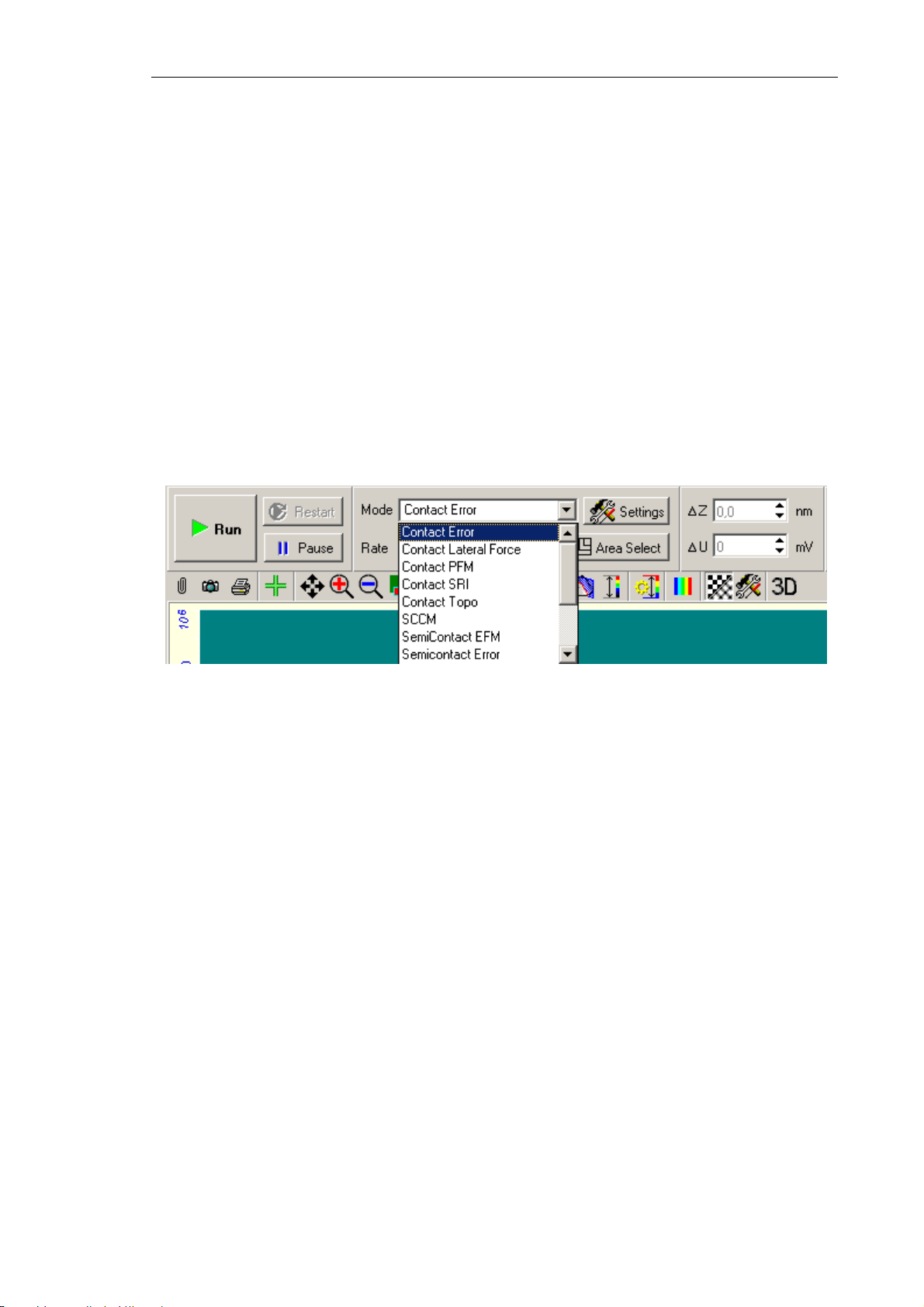
Chapter 7. Performing Measurements
7.1.4.2. Preparation for Measurements
The Contact Error Mode is based on the Constant Force Mode, which is described in detail
in i. 7.1.1 “Constant Force Mode” on page 55.
Before the Contact Error Mode measurements, prepare for the measurements and perform
measurements of surface topography by the Constant Force Mode.
After the completion of preliminary measurements of surface topography by the Constant
Force Mode, perform setting of parameters for operating by the Contact Error Mode.
7.1.4.3. Scanning
Select the Contact Error mode in the Mode list on the Control panel of the Scanning
window (Fig. 7-32). For this cofiguration, the DFL signal will be used as the second
detection signal for the first scan pass.
Fig. 7-32. Selecting the
Contact Error Mode
Click the button Run to trigger the process of scanning.
The following actions take place:
● Line-by-line scanning of the sample surface starts and two images appear in the field of
2D visualization of the scanning data. One of the images is an image of surface
topography (signal
Height), while the other one is the error signal (signal DFL)
(Fig. 7-33);
77
Page 86
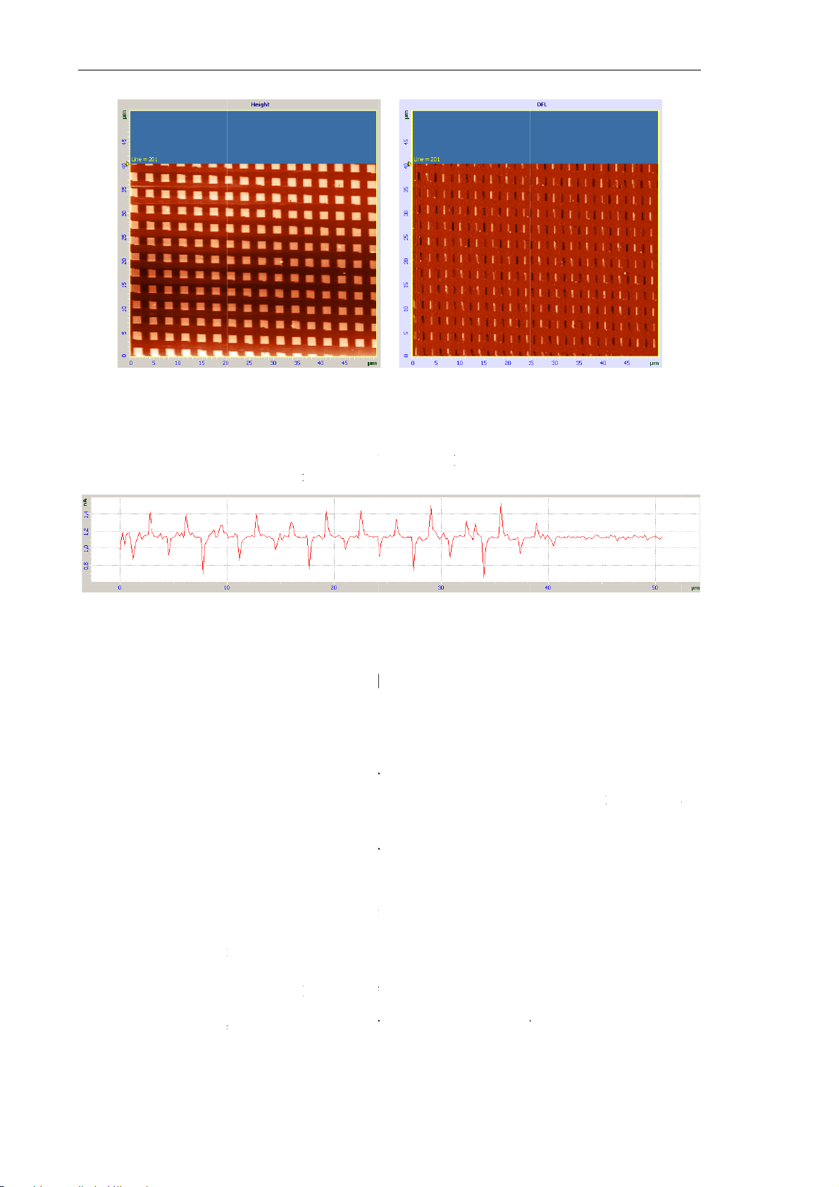
Solver NE
X
S
e
o
i
f
d
c
e
l
o
c
d
r
r
a
e
D
e
l
e
g
e
l
m
t
o
e
u
s
n
i
o
t
t
l
a
u
w
m
t
p
e
w
n
M
a
p
m
fi
a
p
m
n
p
e
v
a
p
(
L
p
n
a
r
e
f
i
m
p
e
a
e
o
e
s
e
f
e
w
e
a
i
r
fe
e
i
g
l
e
l
a
s
l
a
p
h
t
r
t
●
If the
the det
T SPM. Inst
Fig.
button in
ction sign
uction Man
7-33. Image
the left bot
l of selecti
al
of surface
tom of the
g image i
topography
indow is
real time
nd the
Err
ressed, th
Fig. 7-34).
r
signal
1D View
r will disp
ay
7.1.5.
7.1.5.1.
Piezoresp
ferroelectr
the field o
modes of
The intera
(with subs
mode. Thi
form of a
it. Variati
the electri
In this mo
field unde
same local
Piezor
Brief
nse Forc
cs and it a
applied r
ata readin
tion betw
quent ana
s displace
inear relati
ns of the s
field and
e, a bias v
the probe
electric fi
sponse
escript
Microsc
lows inves
search for
/writing re
en the loc
ysis of res
ent results
onship bet
ample geo
he polariza
ltage is ap
. As ferroe
ld to differ
Fig. 7-34
Force
on of th
py is usu
igations of
he develo
ated to the
l electric
lting displ
from the
een the sa
etry depe
ion vector
lied to th
lectrics ha
nt areas of
. Signal DF
icrosco
e Mode
lly used i
their dom
ment of fe
.
eld and th
cements o
iezo-electr
ple geom
d on the
of the sam
conductiv
e the dom
the surfac
y
material
in structur
roelectrics
surface o
the surfac
c effect,
etry and th
agnitude
le.
probe. Th
in structu
yields dif
ciences in
. Especial
data stora
a piezo-e
) lies in th
hich revea
electric fi
nd mutual
s induces
e, the appl
rent result
the study
nterest lies
e devices
ectric sam
basis of t
s itself in
eld applied
orientation
local elect
ication of
.
of
in
nd
le
is
he
to
of
ic
he
78
Page 87
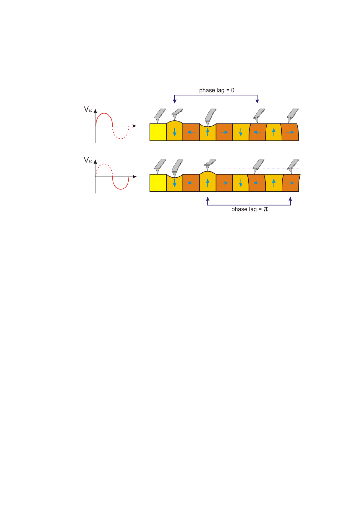
Chapter 7. Performing Measurements
Fig. 7-35 illustrates displacements of the structure whose domains are oriented both
vertically and horizontally. The case of the altering electric field is considered. Oscillations
of the surface are shown both for the positive direction of the electric field, above, and for
the negative, below.
Fig. 7-35
Provided that domains have the same sizes, the magnitude of surface oscillations is the
same. Correspondingly, the magnitude of the cantilever normal deflection is also the same.
However the oscillation phase will be different for those domains with different orientation
of the polarization vector.
In the case of horizontally oriented domains, surface displacements will be lateral with
respect to the surface rather than normal. Respectively, the magnitude of normal
oscillations of the cantilever is equal to zero. However, due to friction between the tip and
the sample surface, some displacement of the tip will occur and, also, its orientation to the
surface will be changing. At the same time, as in the case of normal oscillations, phase of
lateral oscillations depends on the direction of the polarization vector of the domains
oriented horizontally.
Therefore, Piezoresponse Force Microscopy yields both surface topography images and
distributions of amplitudes of lateral and normal oscillations. In addition, the user obtains
phase distributions of lateral and normal oscillations (Fig. 7-36). This information makes it
possible to study the domain structure of the sample under investigation.
79
Page 88
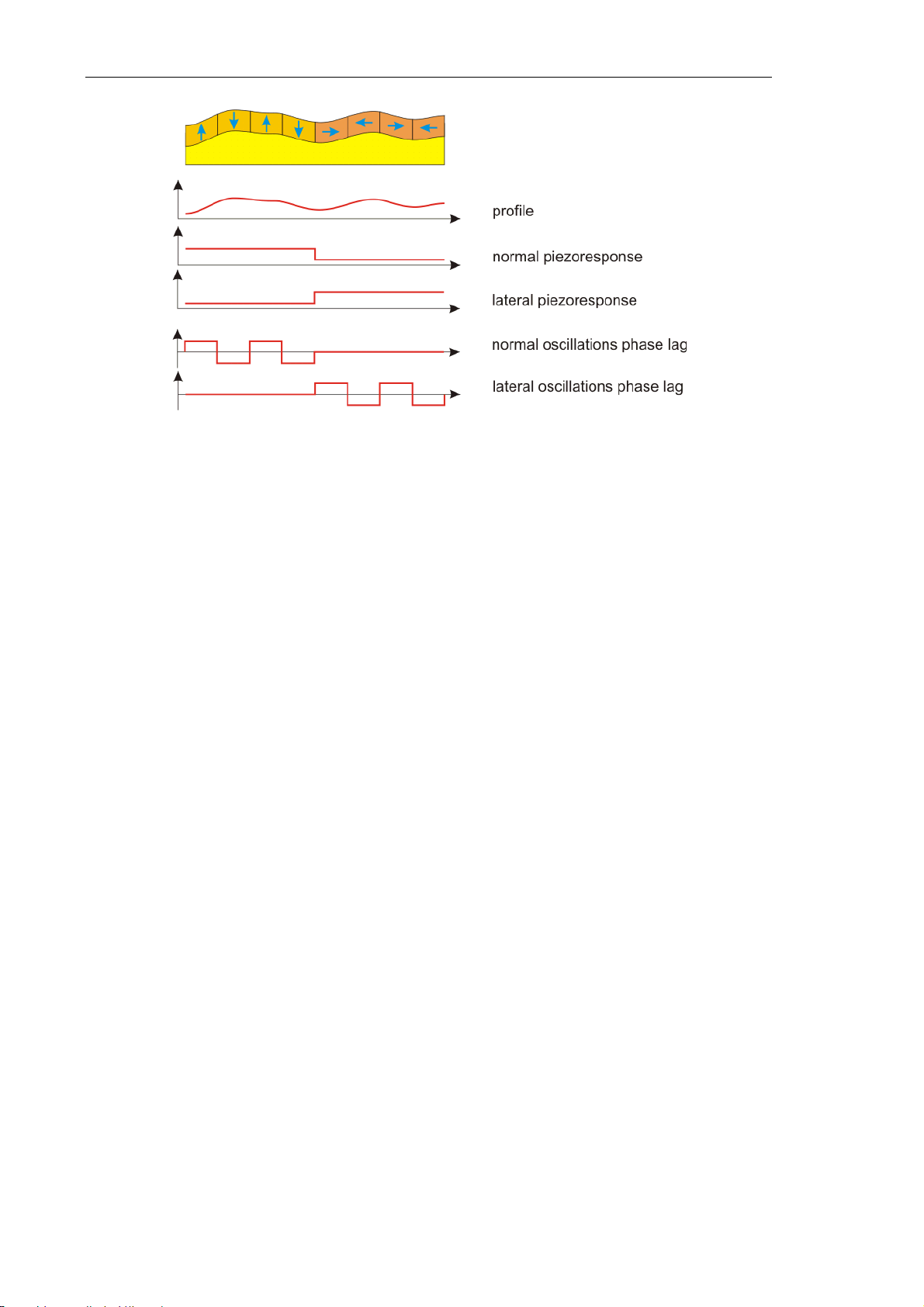
Solver NEXT SPM. Instruction Manual
Fig. 7-36
However interpretation of the results obtained is not always simple. It is necessary to
consider a number of factors which can affect or influence images obtained during
measurements.
For better signal (oscillation amplitude), it is desirable to operate on a frequency that is
close to the frequency of the system cantilever-probe-surface (so that oscillations of the
cantilever pressed to the sample would be resonance). This approach is, however, good
only for homogeneous materials. If the sample is inhomogeneous, containing some
inclusions, for example, the resonance oscillation amplitude will reflect the distribution of
surface elasticity in addition to the domain structure. In this case it is recommended to
operate on a frequency that is afar from the resonance.
For inhomogeneous materials, under certain conditions, the oscillation amplitude can
reflect the sample structure even afar from the resonance. This might be due to camber of
the surface induced by electrostatic forces.
7.1.5.2. Preparation for Measurements
To operate in Piezoresponse Force Microscopy a sample should be glued to the substrate
with the conductive glue or mounted on the substrate with a spring contact and it should be
used conductive probes for contact modes.
Before the Piezoresponse Force Microscopy measurements, prepare for the measurements
and perform measurements of surface topography by the Constant Force Mode.
After the completion of preliminary measurements of surface topography by the Constant
Force Mode, perform setting of parameters for operating on Piezoresponse Force
Microscopy.
80
Page 89
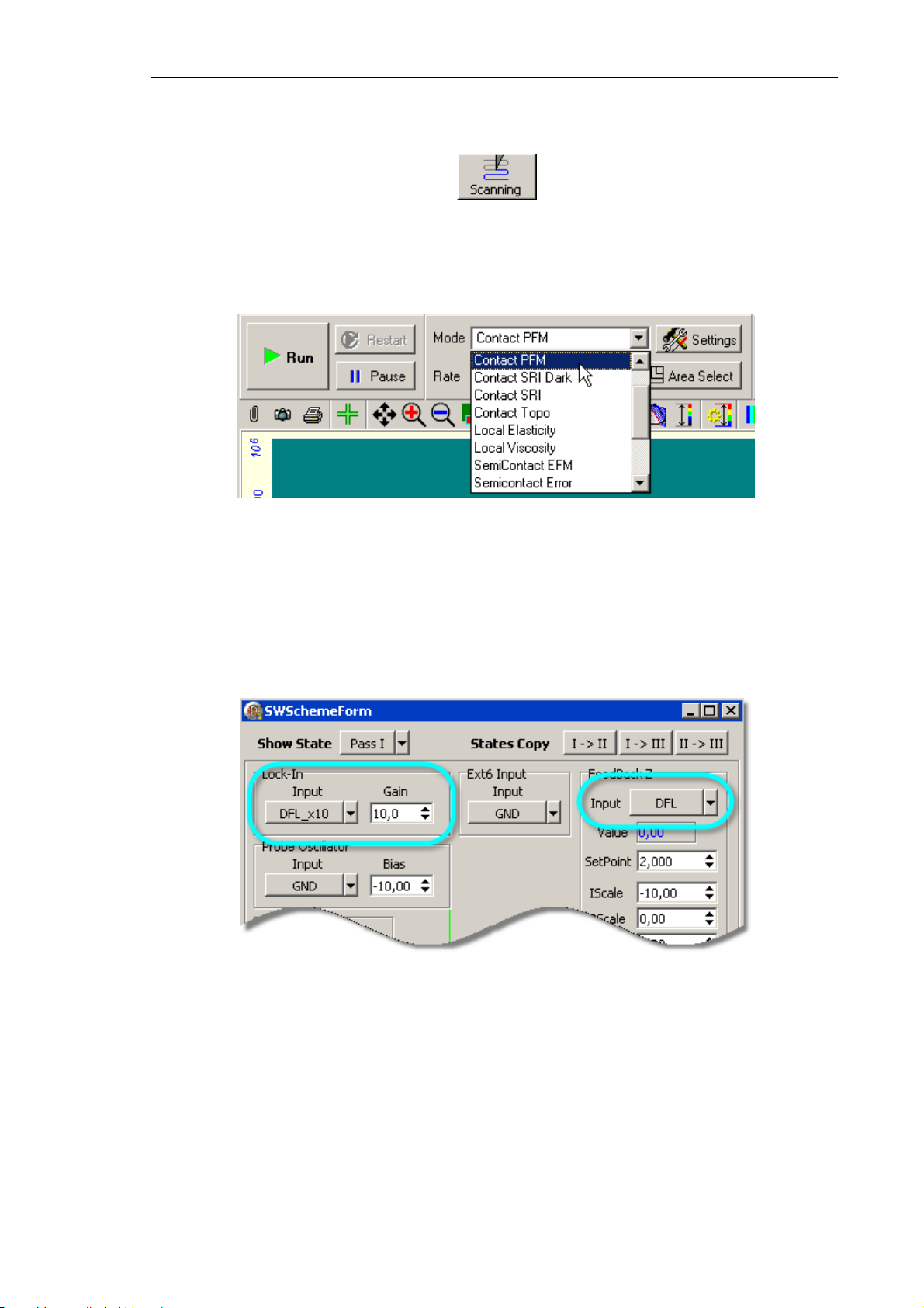
Chapter 7. Performing Measurements
7.1.5.3. Adjusting Scanning Parameters
1. Open the scanning window with the button in the Main Operations panel.
2. Choose the mode Contact PFM from the list Mode on the control panel of the scanning
window (Fig. 7-37). This results in automatic performing all necessary switching
sequences in the controller.
Fig. 7-37. Selection of the Piezoresponse Force Microscopy mode
NOTE. When selecting this mode, the signal
system sets the maximum value for gain coefficients of the lock-in amplifier,
DFL
is automatically connected to the input,
Gain
(Fig. 7-38). Also, the following signals will be selected for measurement during scanning:
Height, Mag
, and
Phase
on the forward pass.
Fig. 7-38
81
Page 90
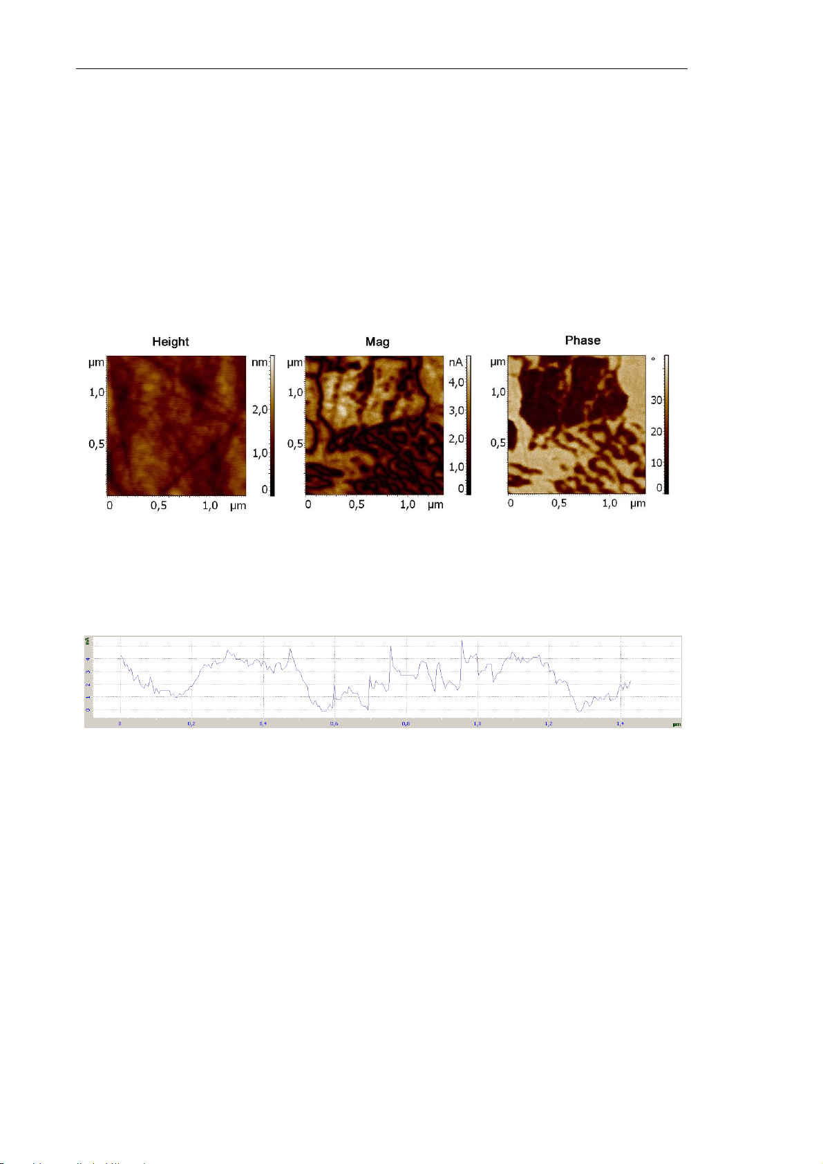
Solver NEXT SPM. Instruction Manual
7.1.5.4. Scanning
Click the button Run, which is on the control panel of the Scan tab, to trigger the process
of scanning.
The following actions take place:
● Line-by-line scanning of the sample surface starts and three images appear in the field
of 2D visualization of the scanning data. One of them is an image of surface
topography (signal Height), the second image is the amplitude of normal oscillations
(signal Mag) and the third one is the distribution of normal phase (signal Phase)
(Fig. 7-39).
Fig. 7-39. Images of the surface under investigation
● The panel of 1D images visualizes the signal measured line-by-line (Fig. 7-40).
Fig. 7-40. Signal Mag
NOTE. Normal oscillations of the cantilever (signal
DFL
) are registered for the default
settings in the Piezoresponse Force Microscopy mode. For registration of lateral
oscillations, connect the input of the lock-in amplifier to the LF (
LF×10
) signal.
82
Page 91
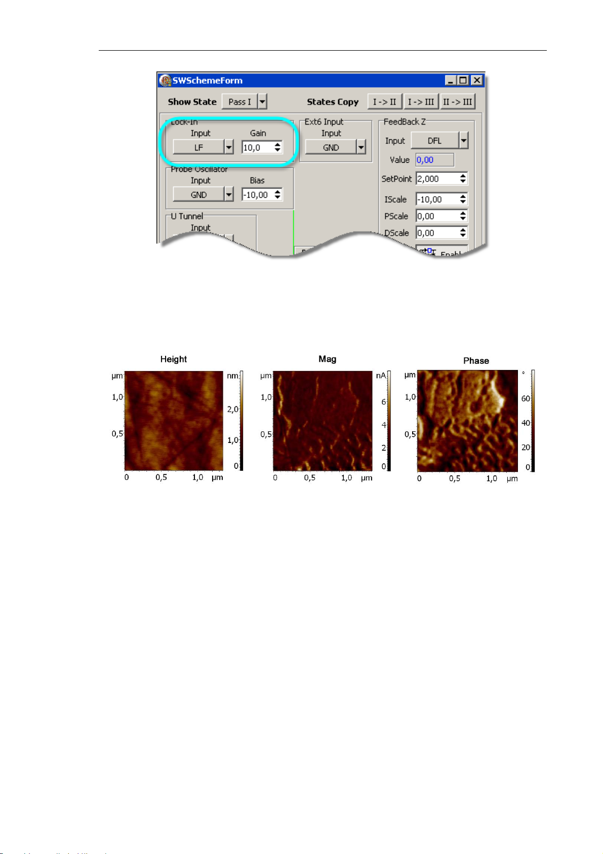
Chapter 7. Performing Measurements
Fig. 7-41
After switching the inputs of the lock-in amplifier and the phase detector from DFL to LF,
the second image of the scanning 2D data visualizes the distribution of the lateral
oscillations amplitude, while the third image is the distribution of lateral phase (Fig. 7-42).
Fig. 7-42. Images of the surface under investigation
83
Page 92

Solver NEXT SPM. Instruction Manual
7.2. Semicontact AFM
7.2.1. Semicontact Mode
Operations performed in measurements of surface topography with the Semicontact
Atomic Force Microscopy of different modes have much in common with those of other
techniques based on resonant oscillations of the cantilever.
Initial state
The following steps are assumed to be done:
● Launching the control program;
● Turning the instrument on;
● Installing the probe;
● Adjusting the cantilever deflection detection system;
● Mounting the sample;
● Moving the measuring head to its working position;
● Initial approach;
● Selecting the scan area.
For details on these operations see Ch. 6 Preparing for Measurements on p. 29.
Procedural Sequence
Measurement in a Semicontact mode is arranged in the following procedural sequence:
1. Adjusting the Controller Configuration (see i.. 7.2.1.1 on p. 85)
2. Adjusting Piezodrive Parameters (see i.. 7.2.1.2 on p. 85)
3. Approaching the Sample to the Probe (see i.. 7.2.1.3 on p. 89)
4. Adjusting Working Level of the Feedback Gain (see i.. 7.2.1.4 on p. 91)
5. Adjusting Scanning Parameters (see i.. 7.2.1.5 on p. 92)
6. Scanning (see i.. 7.2.1.6 on p. 97)
7. Saving Measurement Data (see i.. 7.2.1.7 on p. 100)
8. Completing Measurements (see i.. 7.2.1.8 on p. 101)
These procedures are explained below.
84
Page 93
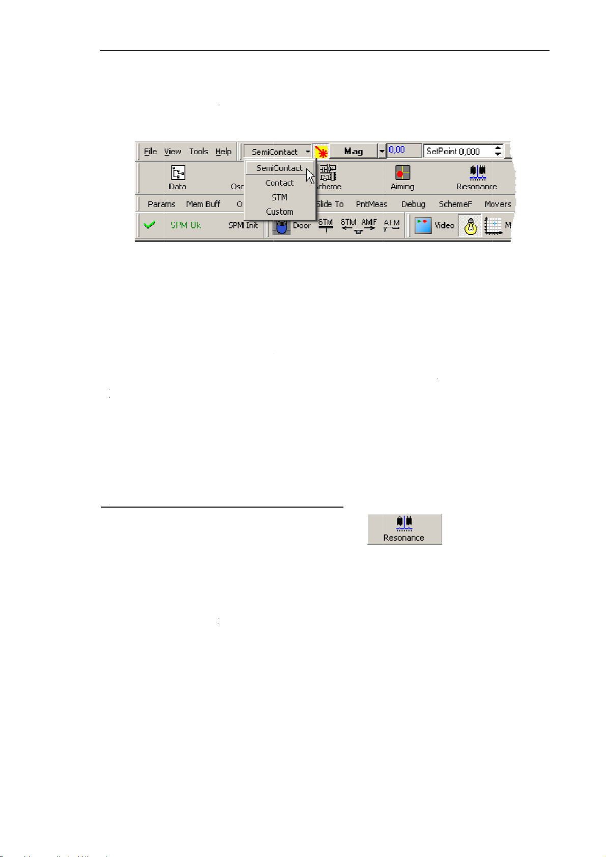
7
wth
n
7
hpaThau
A
n
r
o
o
h
c
ge
e
n
o
e
h
e
a
e
e
n
fo
t
n
n
r
c
a
a
T
a
c
butt
m
e
r
4
o
g
e
e
c
o
o
(
n
a
w
d
b
r
a
r
c
,
o
a
e
n
a
a
n
c
e
h
s
C
u
i
b
n
h
m
rs
i
n
s
w
e
m
d
j
g
hapter 7. P
e
e
M
n
t
f
p
s
s
i
r
n
e
m
m
r
j
p
n
t
n
r
o
s
5
n
e
.
h
,
n
.
d
e
e
gs
rforming M
asurement
.2.1.1.
S
itch the i
e controlle
O
nce the c
i
strument t
.2.1.2.
Adjusti
strument
configura
nfiguratio
operate in
Adjusti
g the C
r operatin
ion list (se
Fig. 7-43. S
SemiCon
semiconta
g Piez
ntrolle
in the Co
Fig. 7-43)
lecting the
tact
is set
t modes pr
drive P
Config
tact techn
at the top
ontroller co
all switc
ceed auto
ramete
ration
que by sel
ar of the
figuration
ing seque
atically.
cting
Se
ain Progra
ces requi
iContact
window.
ed for th
i
O
utput of t
C
aracteristi
rameters o
e Control
tomatic an
djusting
1.
Open th
Operatio
2.
In the dr
Click th
type of t
Paramet
viewed
adjustabl
option (s
e generato
s of the
f the gener
program
d manual.
nerator p
Resonan
s panel.
p-down lis
Reset
e probe.
rs of auto
nd, if nec
paramete
e Fig. 7-4
feeds the
antilever
tor output
llows for
hese optio
rameters
e
windo
t of the
Fin
on to ena
atic adju
ssary, cor
s panel th
).
piezodriv
scillation
frequency,
two optio
s are expl
utomatic
by clicki
Resonan
le paramet
stment of
ected in t
t is acces
that prov
during sca
magnitude
s of adju
ined belo
lly
g the
e
panel, s
rs of auto
the piezo
e
Auto
ad
ible throu
des oscilla
ning proc
, phase shi
ting the
.
lect the de
atic adju
rive work
ustable pa
h selectio
ion of the
ess are ad
t).
iezodrive
button i
ired type o
tment for
ng freque
ameters g
of the
M
cantilever
usted wit
arameters
the Mai
f the probe
he selecte
cy can b
oup of th
re settin
8
Page 94
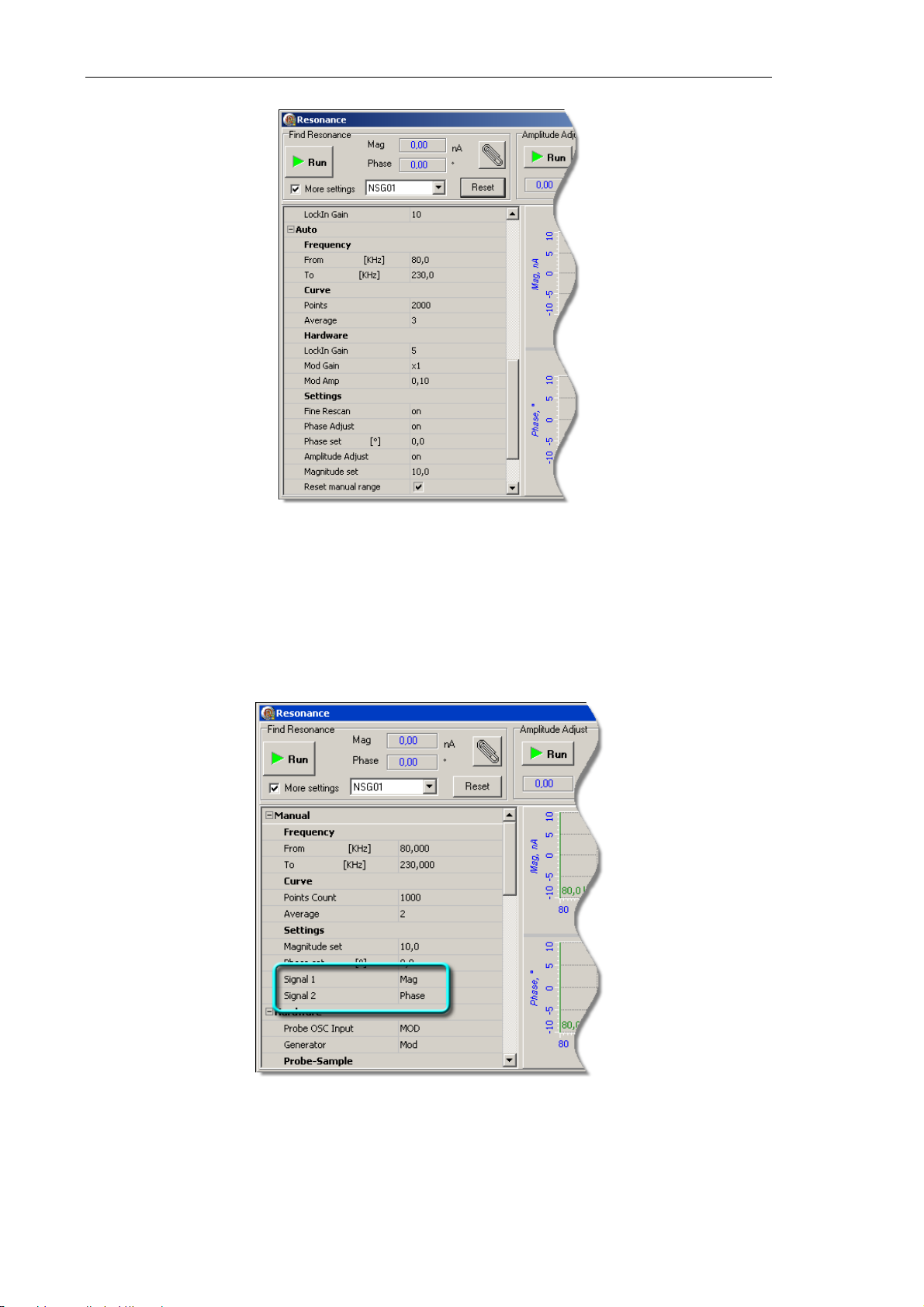
Solver NEXT SPM. Instruction Manual
Fig. 7-44. Piezodrive adjustable parameters panel
NOTE. To display frequency responses of the signals
corresponding options in the
Settings
subgroup of the
Manual
Signal 1 Mag
Signal 2 Phase.
Mag
and
Phase
, select the
parameters group:
3. Before automatic search for the resonance frequency, deselect the More settings option
in the
Find Resonance panel (see Fig. 7-45).
86
Page 95
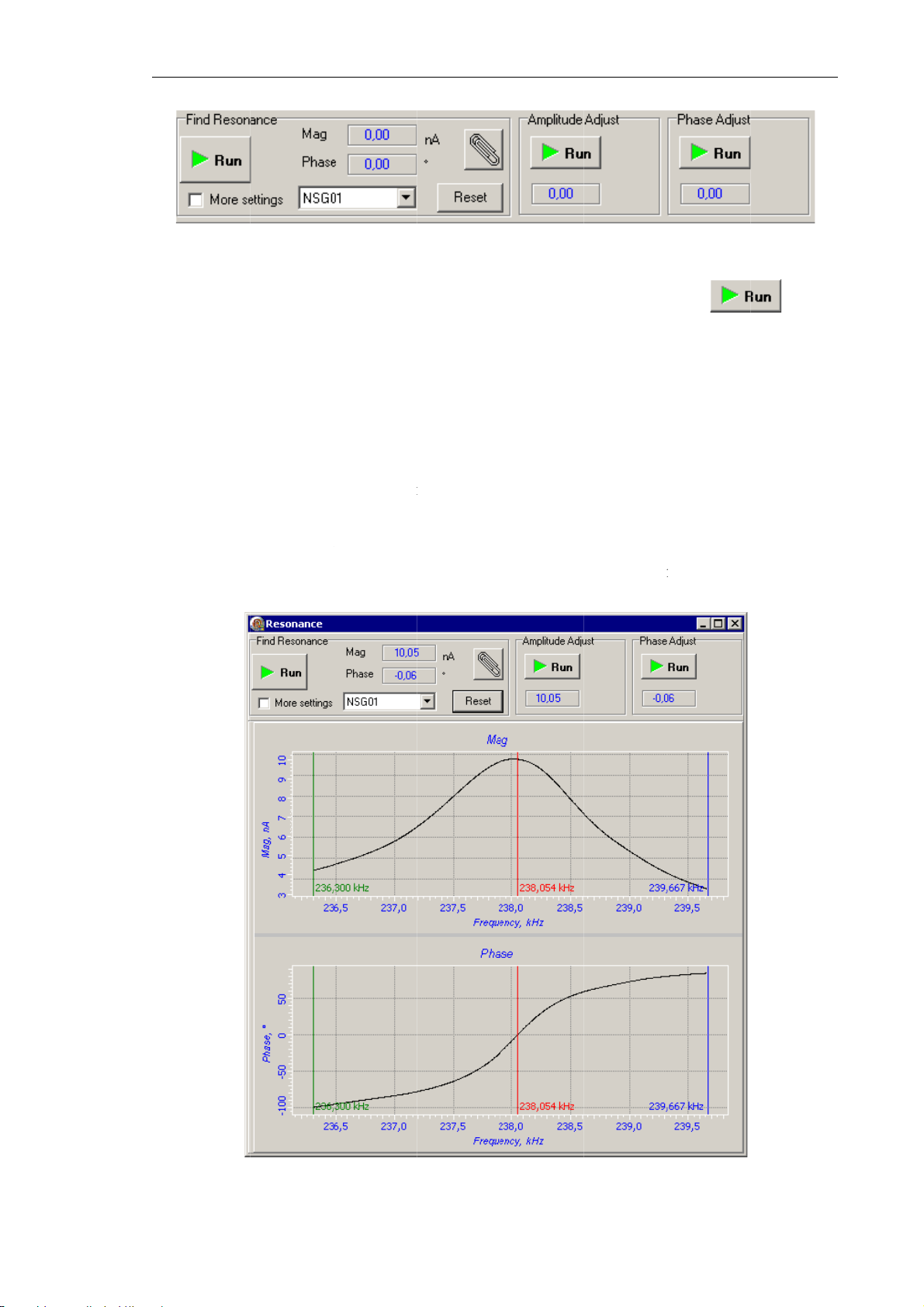
a
n
s
n
s
s
l
m
s
Fi
g
a
e
a
a
h
c
e
o
e
p
e
s
o
r
e
i
o
5
h
t
q
u
m
i
b
g
7
C
a
m
l
e
e
h
P
e
w
k
g
w
e
pnd
n
e
o
i
g
s
7
n
e
e
t
e
. 7-45. Con
trol panel of
the
Reson
hapter 7. P
nce
windo
rforming M
asurement
4. To start
in the
Fi
●
Acqu
(
Pha
●
Findi
●
Adju
●
Adju
canti
para
●
Adju
●
Plotti
reson
utomatic a
d Resonan
iring of fre
e
signal) o
g of the c
ting the pi
ting the g
ever oscill
eter);
ting the p
ng frequen
ance frequ
djustment
ce
panel (s
quency res
f the cantil
ntilever re
zodrive w
in (
LockIn
tion at the
ase shift to
y respons
ncy (see F
f the piez
e Fig. 7-4
onses of t
ver oscilla
onance fre
rking freq
Gain
para
esonance
the prescri
s of the si
g. 7-46).
drive para
). This wil
e magnitu
ion;
uency;
ency to th
eter) to th
s equal to t
ed value (
nals
Mag
a
eters, clic
provide:
de (
Mag
resonance
level at
e prescrib
hase Set
Phase
the
si
nal) and
frequency;
hich magn
d one (
arameter);
i
the range
f the phas
tude of th
Ma
nitude Se
around th
butto
Fig.
-46
8
Page 96
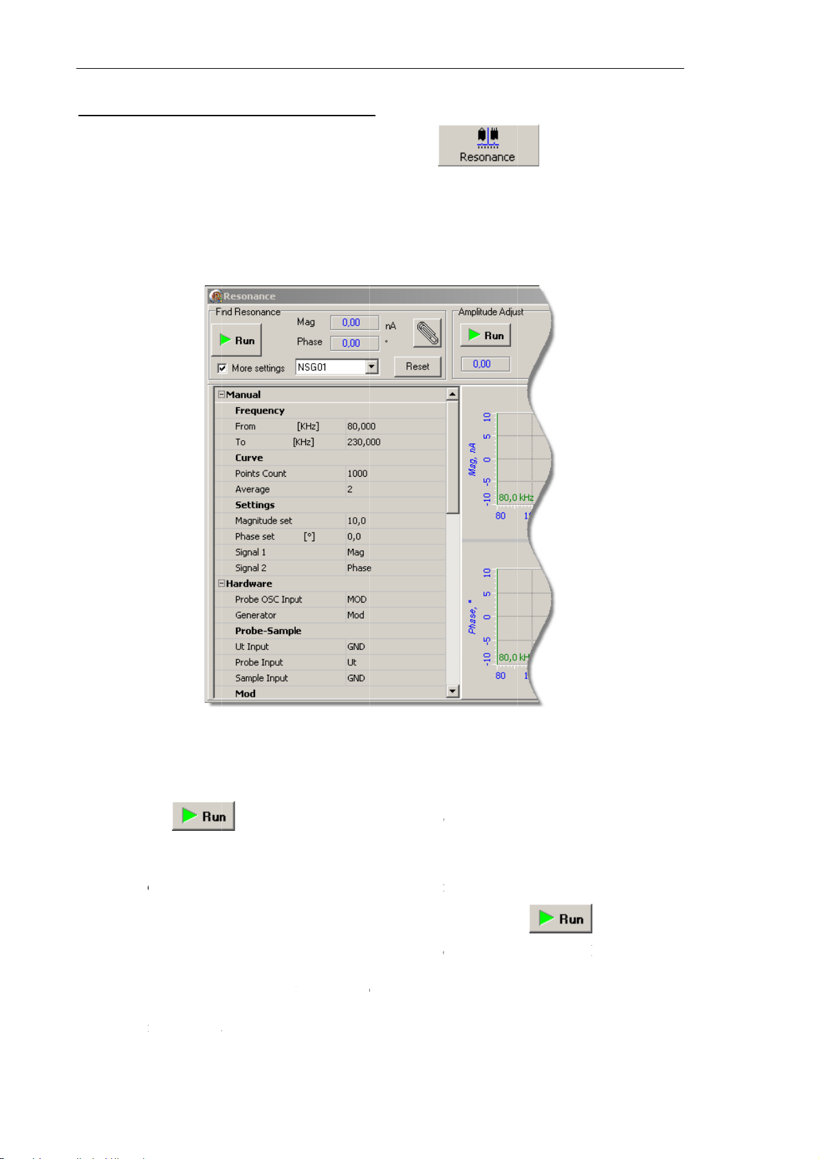
Solver NE
X
t
d
t
f
t
e
a
t
s
o
t
n
x
a
n
r
g
a
b
e
a
n
m
r
n
e
r
v
t
e
a
u
r
o
F
n
o
P
t
l
n
n
r
i
d
y
p
y
a
m
t
d
e
R
h
r
g
n
e
p
u
b
r
e
n
n
r
e
.
a
d
j
e
n
d
i
e
d
e
m
u
s
e
e
n
u
e
k
p
h
y
u
o
a
b
t
4
n
u
n
v
t
e
T SPM. Inst
uction Man
al
Adjusting
1. Open
Operat
2. In the
Click
type o
3. Select
enerator
he
Reson
ions panel.
rop-down
he
Reset
the probe.
he
More s
paramete
nce
wind
list of the
utton to e
ttings
opti
s manuall
w by clic
ind Reson
able para
n to open
king the
nce
panel,
eters of a
he adjusta
select the
tomatic ad
le paramet
button
esired typ
ustment fo
rs panel (s
in the M
of the pro
r the selec
e Fig. 7-4
in
e.
ed
).
Param
necess
4. Click
he
respon
5. Using
colors
6. Repea
measurem
7. Adjust
freque
its ma
adjust
positio
ters for m
ry, the no
es of the
the marke
f the begi
the gene
cy by mo
imum in
ble param
of the m
Fig. 7-47.
nual adjus
-default va
button i
agnitude a
s, select a
ning and o
nt of the f
ator work
ing the re
he vicinit
ters grou
rker.
iezodrive a
ment of th
ues can be
the
Find
d of the p
narrower
f the endin
equency re
ng freque
marker to
of the sel
will dis
justable pa
generator
entered.
esonanc
ase shift i
ange arou
markers a
sponses by
cy (
Frequ
the positio
cted peak
lay the v
ameters pa
are define
panel. Th
the presel
d the reso
e green an
clicking th
ncy
para
n at which
The
Freq
lue corre
el
in the
Ma
s will acq
cted frequ
nance pea
blue, res
eter) at t
the
Mag
enc
inp
ponding t
ual
ire freque
ncy range.
. By defa
ectively.
button.
e resona
si
gnal achie
t field of
the curr
group.
If
cy
lt,
ce
es
he
nt
88
Page 97
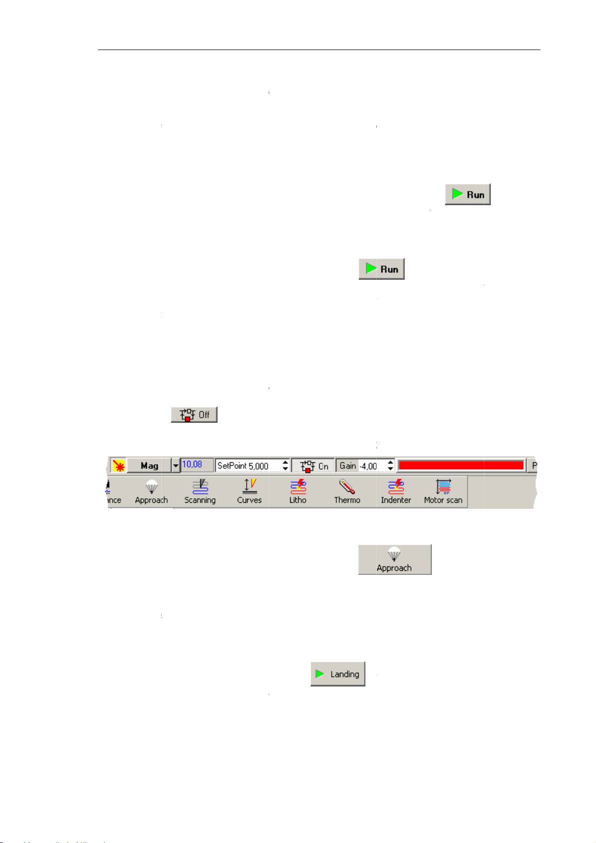
8.
7
o
h
r
d
e
o
Amp
G
a
t
e
r
e
n
n
e
n
h
e
=
h
A
h
e
A
e
t
a
u
e
s
e
e
)
h
c
s
o
A
h
t
e
p
s
p
e
m
A
M
Tter
r
m
l
e
b
n
i
r
i
w
4
l
n
m
n
o
g
h
i
n
e
t
b
m
-
e
n
C
s
c
o
c
a
a
h
t
P
n
e
s
g
d
a
d
bu
e
t
f
a
o
h
t
c
o
r
c
b
t
P
e
e
e
d
w
l
n
h
v
(
d
n
n
–
p
s
9
e
)
e
n
r
d
t
h
t
s
n
n
r
e
Adjust t
generato
or with a
e desired l
voltage (
justing th
vel of the
mplitude
gain of th
Mag
arameter i
lock-in a
signa
. This can
the
Mod
plifier (
Lo
hapter 7. P
be done ei
ubgroup o
kin Gain
rforming M
her with a
the
p
rameter).
Hard
asurement
justing th
are
group
The gen
adjusted
The gain
To set th
the
(
Lockin
value (
To adjus
9.
panel (se
the phas
paramete
.2.1.3.
T
approach
1.
Press th
extensio
the Scan
rator outpu
nly manu
can be adj
e desired l
litude Adju
ain
param
M
nitude S
the phase
e Fig. 7-45
shift of t
).
Approa
the sample
of the Z
er extensi
defines a
lly in the
sted either
vel of the
t
panel.
) to the
t
paramete
shift auto
. This wil
e cantileve
hing th
to the pro
button i
canner to
n indicato
plitude of
mplitude
i
manually
a
signal
his will
level at w
).
atically, cl
adjust the
r oscillatio
Sampl
e, perform
the top
ts maximu
(see Fig. 7
the generat
put field.
r automati
automatic
adjust the
ich the
M
ck the
phase of t
achieves
to the
he followi
ar to clos
. Progres
48) by de
r oscillati
ally.
lly, click t
gain of
signal a
butt
e generato
he presele
robe
g steps:
the feed
of the ex
ree of the c
n. This vo
e
he lock-i
hieves the
n in the
P
to the le
ted value
ack loop.
ension is
olored filli
tage can b
button i
amplifie
preselecte
ase Adjus
el at whic
Phase Se
This start
isplayed i
g.
2.
Open th
Operatio
Define t
3.
recomm
SetPoint
4.
Define t
Start the
5.
pproac
pproac
s panel.
e
SetPoin
ndation is
Mag
/2).
e initial fe
approach
window (
Fig. 7-4
window
parameter
to take
dback gain
rocedure
ee Fig. 7-
8. Scanner
by clickin
in the inp
ts initial
in the
Gai
ith the
9).
xtension in
g the
t field of
value equ
input fiel
icator
the Main
l half of
to be in th
tton in th
button i
arameters
the
Mag
range of
Control
the Mai
panel. Ou
level (i.e.
2 ÷ –6.
anel of th
8
Page 98
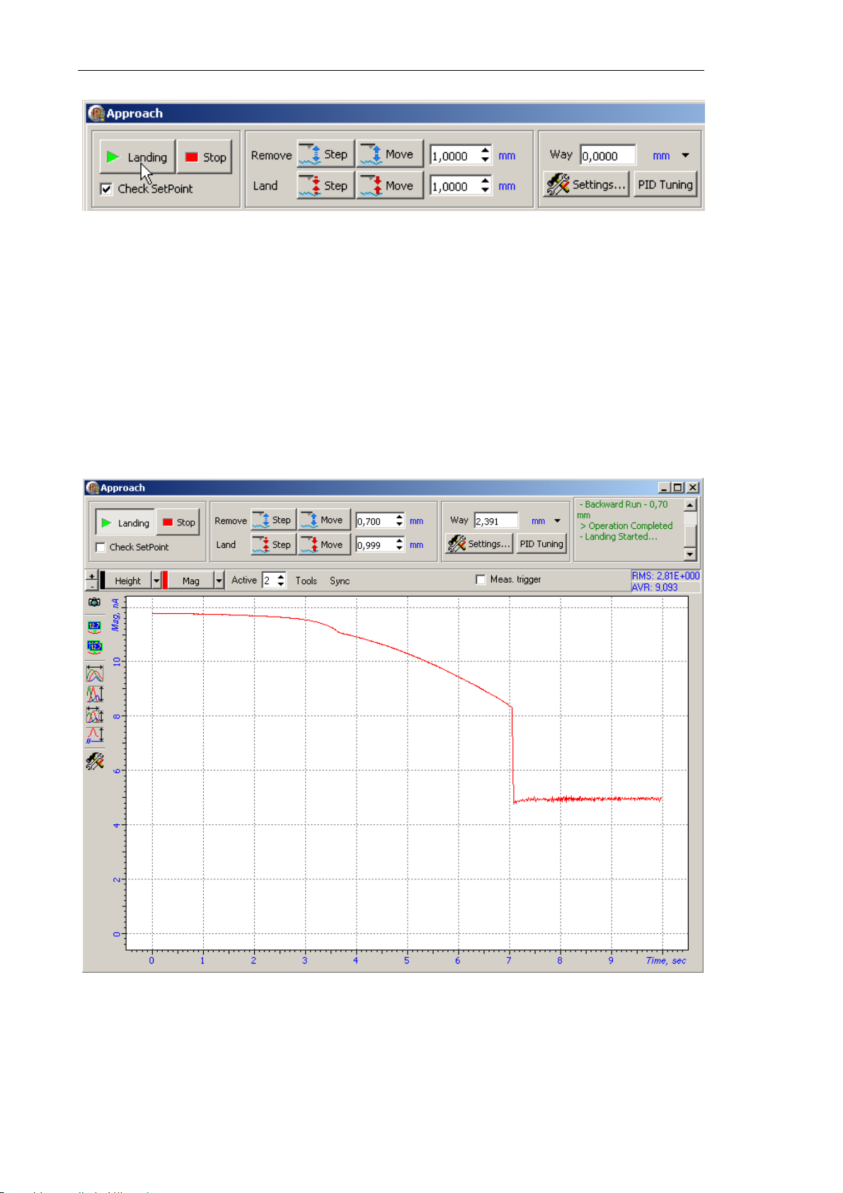
Solver NEXT SPM. Instruction Manual
Fig. 7-49. Control panel of the
Approach window
During the approach procedure, observe variations of the Mag signal in the software
oscilloscope and state of the scanner extension indicator. Wait until the procedure
completes.
Providing the approach parameters are set correctly, the approach procedure completes in
about 10 to 30 seconds and the system goes to following state (see Fig. 7-50):
90
Fig. 7-50. Approach process
Page 99
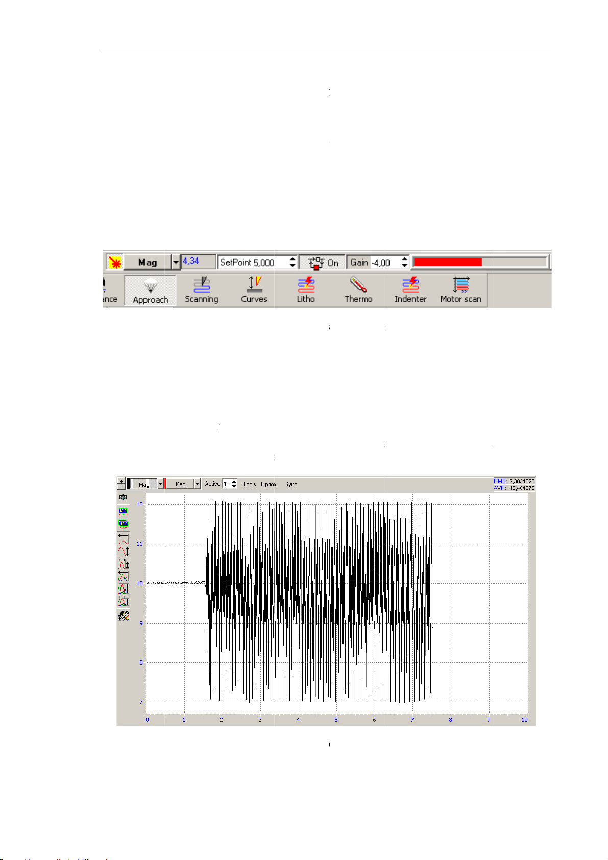
●
7
hprgaun
g
s
t
n
t
a
s
p
f
p
c
e
n
i
l
s
t
n
v
h
r
F
i
g
t
r
i
l
)
r
t
o
h
e
r
n
a
e
g
r
h
o
C
t
a
t
g
h
n
e
F
o
n
e
e
n
g
t
e
c
)
e
e
d
o
t
F
a
h
o
u
s
p
.
r
g
a
k
s
h
The
Ma
maintain
Note tha
extensio
signal d
the Z-sca
this posit
range;
creases to
ner in the
on of the
the level
position w
scanner is
of parame
ere the v
approxima
hapter 7. P
er
Set Poi
lue of
Ma
ely equal
rforming M
t
, the fee
is equal t
o half of
asurement
back loo
Set Point
he scanne
The sof
●
of the
The mes
●
The step
●
Length o
●
.2.1.4.
T
e greater
ocessing s
in (let us
stable and
a
significant
ware osci
M
signal to
age “
er motor i
the indica
Adjusti
is the le
eed in the
all it thres
noise gene
alternating
Landi
loscope d
the
Set Poi
Comple
n
disabled;
or bar dec
Fig.
g Work
el of the
feedback
old value
ation occu
componen
splays th
nt
level;
ed
” appea
eases dow
7-51. Appro
ng Lev
feedback
oop. Neve
, the mode
s. Under t
(see Fig. 7
Mag(t)
s at the rig
to some i
ch complet
l of the
ain (
Gain
theless, at
of operati
is conditio
-52).
raph that
t top of th
termediate
d
eedba
parameter
some high
n of the f
, the
Mag
illustrates
Approach
value (see
k Gain
, the gre
level of t
edback lo
signal is s
decreasin
window.
ig. 7-51).
ter is dat
e feedbac
p become
pplied wit
ig. 7-52. N
ise generati
n in the fe
dback loop
91
Page 100
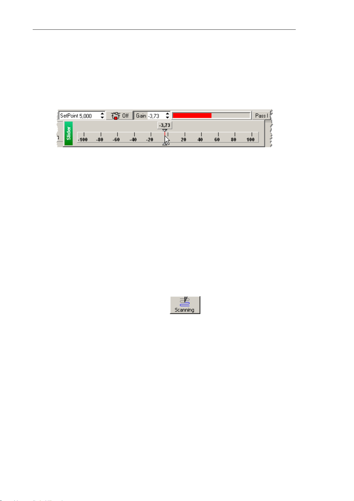
Solver NEXT SPM. Instruction Manual
For stable operation, it is recommended to define the feedback gain to less 0.5÷0.7 of the
threshold value where the noise generation occurs. The feedback gain is adjusted in the
Gain input field.
To adjust the working level of the feedback gain, perform the following steps:
1. Double-click the Gain input field in the Main Parameters panel. The adjusting slider of
the feedback gain will appear (see Fig. 7-53).
Fig. 7-53. Adjusting slider of the
Gain parameter
2. Gradually decrease the Gain level and watch the Mag level in the software
oscilloscope.
NOTE. The
Gain
level should be negative in semicontact modes.
3. Determine the value of the Gain parameter at which noise generation occurs. The
beginning of the generation is identified by appearance of a noticeable alternating
component in the Mag signal (see Fig. 7-52).
4. Increase the value of the Gain parameter to 0.5÷0.7 of the threshold. This value will be
used in further operation.
7.2.1.5. Adjusting Scanning Parameters
Open the Scanning window by clicking the button in the Main Operations
panel.
The top part of the Scanning window contains a panel to control the scanning process
(see Fig. 7-54).
92
 Loading...