

Page 1

SP1 Stereo Vision System
User Manual
(v1.0) August 28, 2015
VI SI ON T EC HN OL OG IE S
Dr. Konstantin Schauwecker
Nerian Vision Technologies
Gotenstr. 9
70771 Leinfelden-Echterdingen
Germany
Email: [email protected]
Page 2

Contents
1 Functionality Overview 3
2 Included Parts 3
3 General Specifications 3
3.1 Hardware Details . . . . . . . . . . . . . . . . . . . . . . . . . . 3
3.2 Stereo Matching . . . . . . . . . . . . . . . . . . . . . . . . . . . 3
3.3 Image Rectification . . . . . . . . . . . . . . . . . . . . . . . . . 4
4 Mechanical Specifications 4
4.1 Dimensions . . . . . . . . . . . . . . . . . . . . . . . . . . . . . 4
4.2 Mounting . . . . . . . . . . . . . . . . . . . . . . . . . . . . . . 4
5 Physical Interfaces 6
6 Hardware Setup 7
6.1 Connecting the SP1 . . . . . . . . . . . . . . . . . . . . . . . . . 7
6.2 Supported Cameras . . . . . . . . . . . . . . . . . . . . . . . . . 7
6.3 Camera Alignment . . . . . . . . . . . . . . . . . . . . . . . . . 8
6.4 External Trigger . . . . . . . . . . . . . . . . . . . . . . . . . . . 8
7 Processing Results 9
7.1 Rectified Images . . . . . . . . . . . . . . . . . . . . . . . . . . . 9
7.2 Disparity Maps . . . . . . . . . . . . . . . . . . . . . . . . . . . 9
8 Configuration 11
8.1 System Status . . . . . . . . . . . . . . . . . . . . . . . . . . . . 11
8.2 Preview . . . . . . . . . . . . . . . . . . . . . . . . . . . . . . . 12
8.3 Processing Settings . . . . . . . . . . . . . . . . . . . . . . . . . 14
8.4 Cameras . . . . . . . . . . . . . . . . . . . . . . . . . . . . . . . 15
8.4.1 Camera Selection . . . . . . . . . . . . . . . . . . . . . . 15
8.4.2 Camera Settings . . . . . . . . . . . . . . . . . . . . . . 16
8.4.3 Recommended Settings for Point Grey Cameras . . . . . 17
8.4.4 Recommended Settings for IDS Cameras . . . . . . . . . 17
8.5 Trigger . . . . . . . . . . . . . . . . . . . . . . . . . . . . . . . . 18
8.6 Camera Calibration . . . . . . . . . . . . . . . . . . . . . . . . . 18
8.6.1 Calibration Board . . . . . . . . . . . . . . . . . . . . . . 18
8.6.2 Recording Calibration Frames . . . . . . . . . . . . . . . 20
8.6.3 Performing Calibration . . . . . . . . . . . . . . . . . . . 21
8.7 Reviewing Calibration Results . . . . . . . . . . . . . . . . . . . 21
8.8 Network Settings . . . . . . . . . . . . . . . . . . . . . . . . . . 24
8.9 Maintenance . . . . . . . . . . . . . . . . . . . . . . . . . . . . . 24
1
Page 3

9 API Usage Information 25
9.1 General Information . . . . . . . . . . . . . . . . . . . . . . . . 25
9.2 ImageTransfer Example . . . . . . . . . . . . . . . . . . . . . . 26
9.3 AsyncTransfer Example . . . . . . . . . . . . . . . . . . . . . . 28
9.4 3D Reconstruction . . . . . . . . . . . . . . . . . . . . . . . . . 29
10 SpCom Sample Application 29
11 Support 31
12 Warranty Information 31
13 Open Source Information 32
2
Page 4

3 GENERAL SPECIFICATIONS
1 Functionality Overview
The SP1 stereo vision system is a stand-alone processing system for performing
stereo matching in real time. It is connected to two industrial USB cameras
that provide input image data. The SP1 correlates the images of both cameras
and produces a disparity map, which is transmitted through gigabit ethernet.
The disparity map describes a mapping of image points from the left camera
image to corresponding image points in the right camera image. With this
information it is possible to reconstruct the 3D location of the corresponding
scene points.
2 Included Parts
When ordering a new SP1 from Nerian Vision Technologies, the package should
include the following parts:
• SP1 stereo vision system
• 5 V DC power adapter
• 4 stickable rubber pads (not included for surface mountable version)
• Manual
If any of the listed parts is missing in your delivery, please contact our
support personnel.
3 General Specifications
3.1 Hardware Details
Power consumption: < 4 W
Power supply: 5 V DC
Dimensions: 105 x 76 x 36 mm
Weight: 0.25 kg
I/O: USB 2.0 host, gigabit ethernet, 2x trigger out
Max. USB power: 500 mA
3.2 Stereo Matching
Stereo algorithm: Semi-Global Matching (SGM)
Disparity range: 112 pixels
Processing rate: 30 Hz
Sub-pixel resolution: 4 bits (1/16 pixel)
Supported image size: 640 × 480 pixels
Post-processing: Consisteny check, uniqueness check,
gap interpolation, noise reduction
3
Page 5
3.3 Image Rectification 4 MECHANICAL SPECIFICATIONS
-
75
?
6
36
(a)
-
75
?
6
36
(b)
-
105
?
6
36
(c)
-
105
?
6
75
(d)
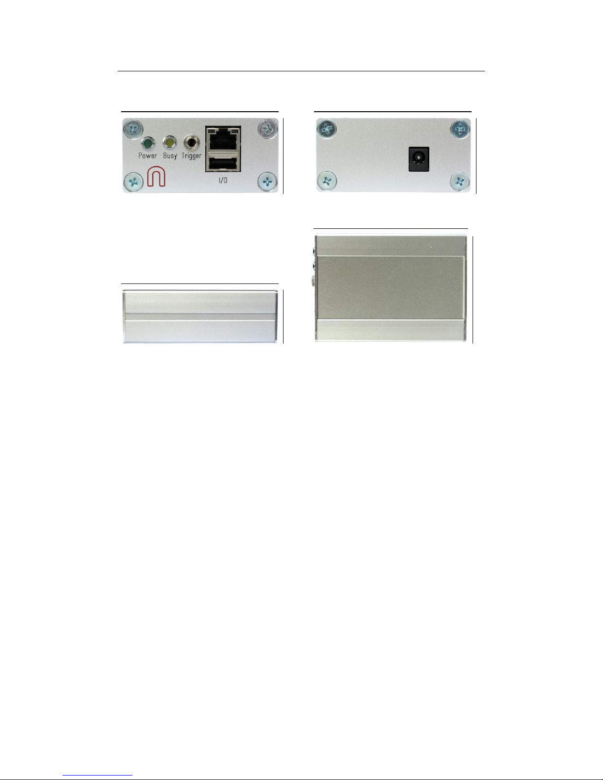
Figure 1: (a) Front, (b) rear, (c) side and (d) top view of SP1 with dimensions
in millimeters.
3.3 Image Rectification
Horizontal displacement: −31 to +31 pixels
Vertical displacement: −31 to +31 pixels
Interpolation: Bilinear
4 Mechanical Specifications
4.1 Dimensions
Figures 1a to 1d show the SP1 as seen from front, rear, side and top. The
provided dimensions are measured in millimeters.
4.2 Mounting
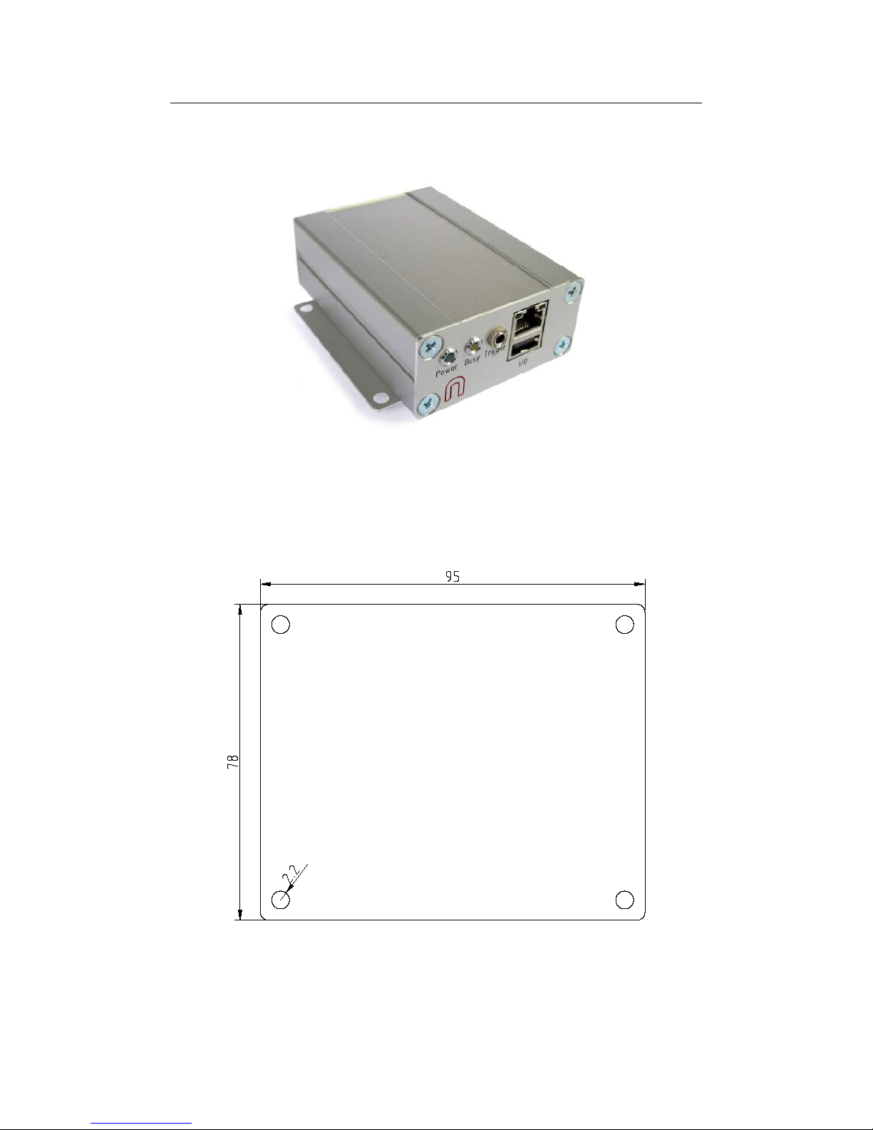
The SP1 is optionally available in a surface mountable version. This version
features a mounting plate that is attached to the bottom side of the housing.
The four through holes on the mounting plate can be used for mounting the
SP1 onto a flat surface. The dimensions of this mounting plate are shown in
millimeters in Figure 3. The through holes are compatible to screws with an
M4 ISO metric thread.
4
Page 6
4.2 Mounting 4 MECHANICAL SPECIFICATIONS
Figure 2: SP1 with attached mounting plate.
Figure 3: Mounting plate dimensions in millimeters.
5
Page 7
5 PHYSICAL INTERFACES
-
Power LED
@
@
@R
Busy LED
A
A
A
A
AU
Trigger port
Ethernet port
USB port
(a)
Power jack
(b)
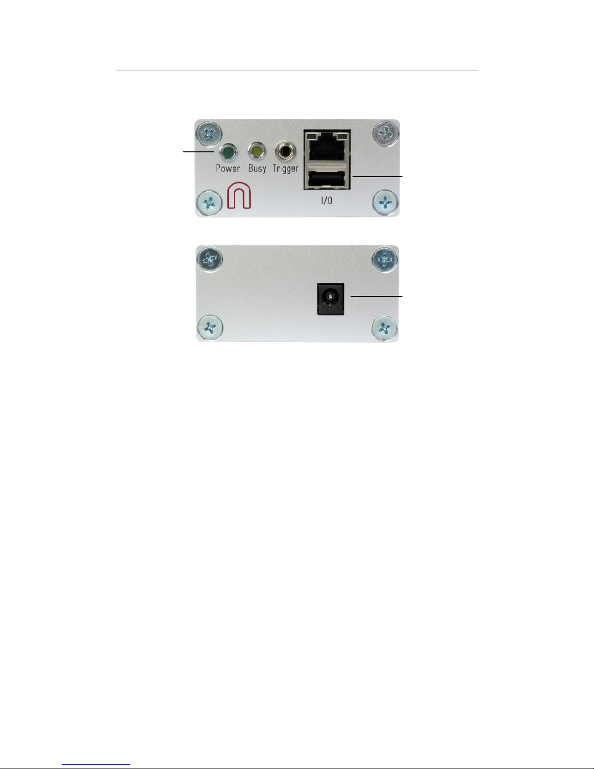
Figure 4: Interfaces on (a) front and (b) rear housing side.
5 Physical Interfaces
Figures 4a and 4b show the interfaces on the SP1’s front and backside. The
power jack is located on the backside, and it needs to be connected to the
supplied power adapter or an equivalent model. When using an alternative
power supply, please make sure that the voltage is set no higher than 5 V DC,
as otherwise the device might be damaged.
The front side features the following interfaces:
Power LED: Indicates that the device is powered up and running.
Busy LED: Indicates that the device is currently processing incoming input
data.
Trigger port: Port for providing two camera trigger signals. See Section 6.4.
Ethernet port: Port for connecting to a client computer. It is used for de-
livering processing results, and for providing access to the configuration
interface.
USB port: Port for connecting the desired USB cameras through a USB hub.
6
Page 8
6 HARDWARE SETUP
USB cameras
Computer
SP1
USB hub
Ethernet
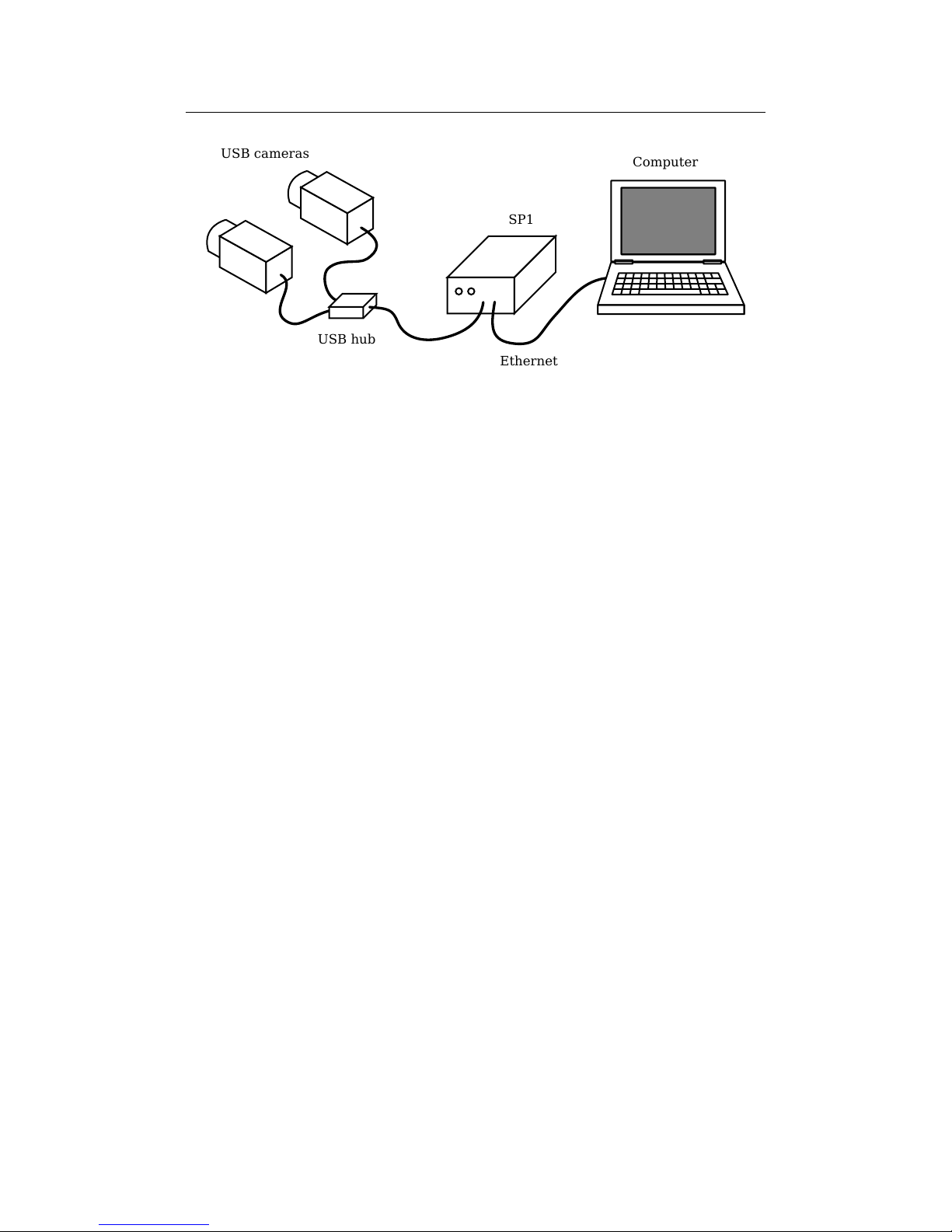
Figure 5: Example setup for cameras, SP1 and client computer.
6 Hardware Setup
6.1 Connecting the SP1
Figure 5 shows a basic system setup for stereo vision. A client computer that
receives the processing results is connected to the SP1’s ethernet port. Alternatively it is possible to connect the SP1 to a switched network. However, you
will have to ensure that the network is capable of handling the high bandwidth
data that is transmitted by the device. The network must support data rates
of at least 25 MB/s.
The cameras are connected to the SP1’s USB port. As the SP1 only features
one USB port, a USB hub is mandatory for making this connection. Please
note that the USB hub usually has to be powered externally, to meet
the power consumption of the cameras.
6.2 Supported Cameras
The SP1 supports the following camera models:
• Point Grey Blackfly; model BFLY-U3-03S2M-CS
• Point Grey Blackfly; model BFLY-U3-13S2M-CS
• Point Grey Chameleon3; model CM3-U3-13S2M-CS
• Point Grey Chameleon3; model CM3-U3-13Y3M-CS
• Point Grey Flea3; model FL3-U3-13E4M-C
• Point Grey Flea3; model FL3-U3-13Y3M-C
• Point Grey Grasshopper3; model GS3-U3-14S5M-C
• Point Grey Grasshopper3; model GS3-U3-15S5M-C
7
Page 9
6.3 Camera Alignment 6 HARDWARE SETUP
Figure 6: Example for standard epipolar geometry.
• IDS uEye ML; model UI-3240ML-M-GL
• IDS uEye CP; model UI-3140CP-M-GL Rev.2
• IDS uEye CP; model UI-3240CP-M-GL
All cameras must have a gray scale sensor.
6.3 Camera Alignment
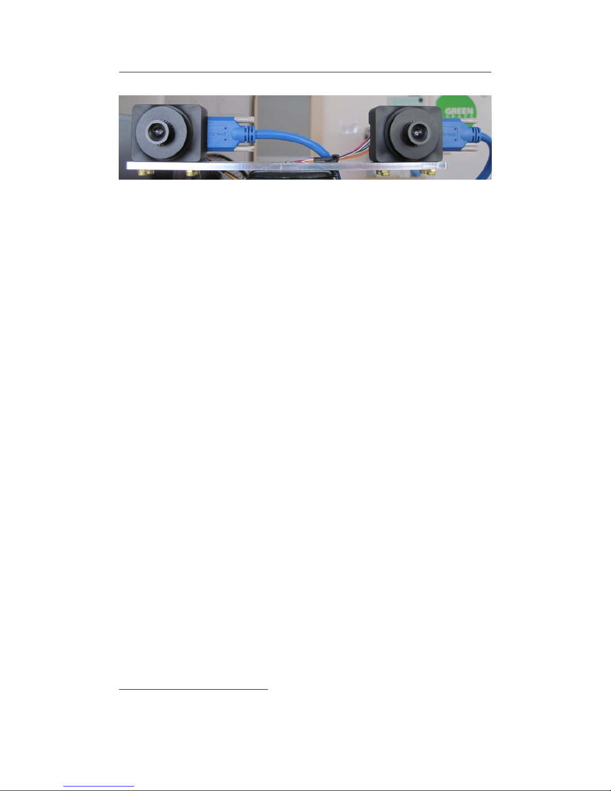
Both cameras have to be mounted on a plane with a displacement that is
perpendicular to the cameras’ optical axes. Furthermore, both cameras must
be equipped with lenses that have an identical focal length. This arrangement
is known as the standard epipolar geometry. An example for such a camera
mounting is shown in Figure 6.
The distance between both cameras is referred to as baseline distance. Using a large baseline distances improves the depth resolution at high distances.
A small baseline distances, on the other hand, allows for the observation of
very close objects. The baseline distance should be adjusted in conjunction
with the lenses’ focal length. An online tool for computing desirable combinations of baseline distance and focal length can be found on the Nerian Vision
Technologies website1.
6.4 External Trigger
For stereo matching it is important that both cameras are synchronized, meaning that both cameras record an image at exactly the same point of time. Many
industrial cameras already feature the ability to synchronize themselves, by
having one camera produce a trigger signal for the respective other camera.
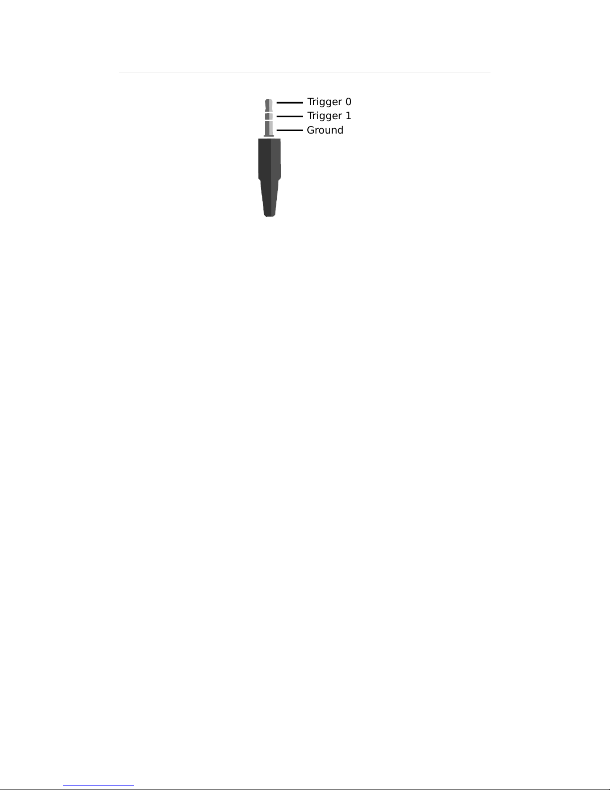
As an alternative, the SP1 can produce up to two trigger signals. The
signals are provided through the trigger port, which can receive a standard
3.5 mm phone connector. The pin assignment for this connector is shown in
Figure 7.
The peak voltage of both trigger signals is at +3.3 V. To protect the trigger
port from short circuits, each signal line is connected through a 220 Ω series
1
http://nerian.com/products/sp1-stereo-vision/calculator/
8
Page 10
7 PROCESSING RESULTS
Ground
Trigger 0
Trigger 1
Figure 7: Pin assignement for trigger output.
resistor. Trigger frequency and pulse width can be configured through the web
interface (see Section 8.5).
7 Processing Results
7.1 Rectified Images
Even when carefully aligning both cameras, you are unlikely to receive images
that match the expected result form an ideal standard epipolar geometry.
The images will be affected by various distortions that result from errors in
the cameras’ optics and mounting. Therefore, the first processing step that
is performed is an image undistortion operation, which is known as image
rectification.
Image rectification requires precise knowledge of the cameras’ projective
parameters. These can be determined through camera calibration. Please refer
to Section 8.6 for a detailed explanation of the camera calibration process.
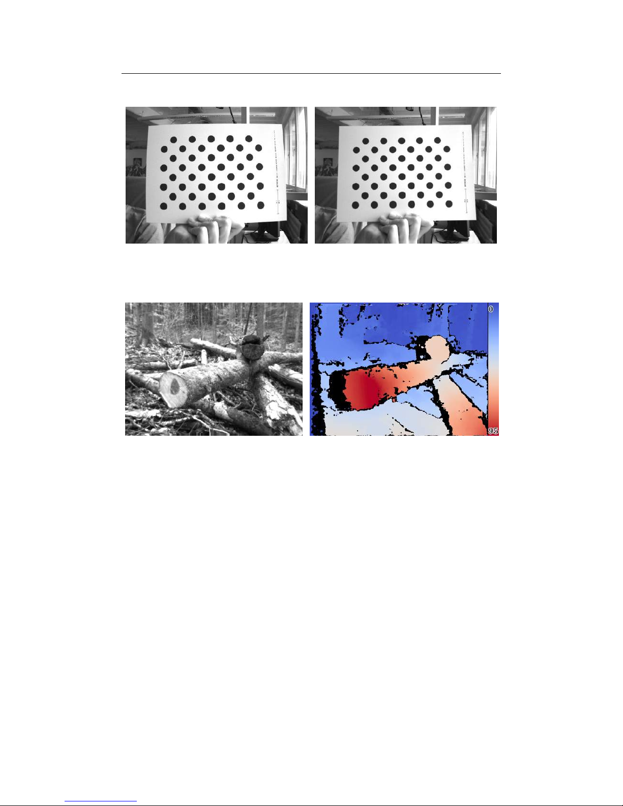
Figure 8a shows an example camera image, where the camera was pointed
towards a calibration board. The edges of the board appear slightly bent,
due to radial distortions in the camera’s optics. Figure 8b shows the same
image after image rectification. This time, all edges of the calibration board
are perfectly straight.
When performing stereo matching, the SP1 additionally outputs the rectified left camera image. This allows for a mapping of features in the visible
image to structures in the determined scene depth and vice versa.
7.2 Disparity Maps
The stereo matching results are delivered in the form of a disparity map for
the left camera image. The disparity map assigns each pixel in the left camera
image to a corresponding pixel in the right camera image. Because both images were previously rectified to match an ideal standard epipolar geometry,
9
Page 11
7.2 Disparity Maps 7 PROCESSING RESULTS
(a) (b)
Figure 8: Example for (a) unrectified and (b) rectified camera image.
(a) (b)
Figure 9: Example for (a) left camera image and corresponding disparity map.
corresponding pixels should only differ in their horizontal coordinates. The
disparity map thus only has to encode the horizontal coordinate difference.
An example for a left camera image and the corresponding disparity map
are shown in Figure 9a and 9b. Here the disparity map has been color coded,
with blue hues reflecting small disparities, and red hues reflecting large disparities. The disparity is proportional to the inverse depth of the corresponding
scene point. It is thus possible to transform the disparity map into a set of 3D
points. This can be done at a correct metric scale if the cameras have been
calibrated.
The transformation of a disparity map to a set of 3D points requires knowledge of the disparity-to-depth mapping matrix Q, which is computed during
camera calibration and can be obtained from the review calibration page of the
SP1’s web interface (see Section 8.7). The 3D location
x y z
T
of a point
with image coordinates (u, v) and disparity d can be reconstructed as follows:
10
Page 12

8 CONFIGURATION
x
y
z
=
1
w
·
x
0
y
0
z
0
, with
x
0
y
0
z
0
w
= Q ·
u
v
d
1
An efficient implementation of this transformation is provided with the
available API (see Section 9.4).
The SP1 computes disparity maps with a resolution that is below one pixel.
Disparity maps have a bit-depth of 12 bits, with the lower 4 bits of each value
representing the fractional disparity component. It is thus necessary to divide
each value in the disparity map by 16 in order to receive the correct disparity
magnitude.
The SP1 applies several post-processing techniques in order to improve
the quality of the disparity maps. Some of these methods detect erroneous
disparities and mark them as invalid. Invalid disparities are set to 0xFFF,
which is the highest value that can be stored in a 12-bit disparity map. In
Figure 9b invalid disparities have been depicted as black.
8 Configuration
The SP1 is configured through a web interface, which can be reached by entering the IP address of the SP1 in your browser. The default address is
http://192.168.10.10. Please configure the IP address and subnet mask of your
computer appropriately, such that this interface can be reached. If the SP1
has just been plugged in, it will take several seconds before the web interface
is accessible.
For using the web interface you require a browser with support
for HTML 5. Please use a recent version of one of the major browsers, such
as Internet Explorer, Firefox, Chrome or Safari.
8.1 System Status
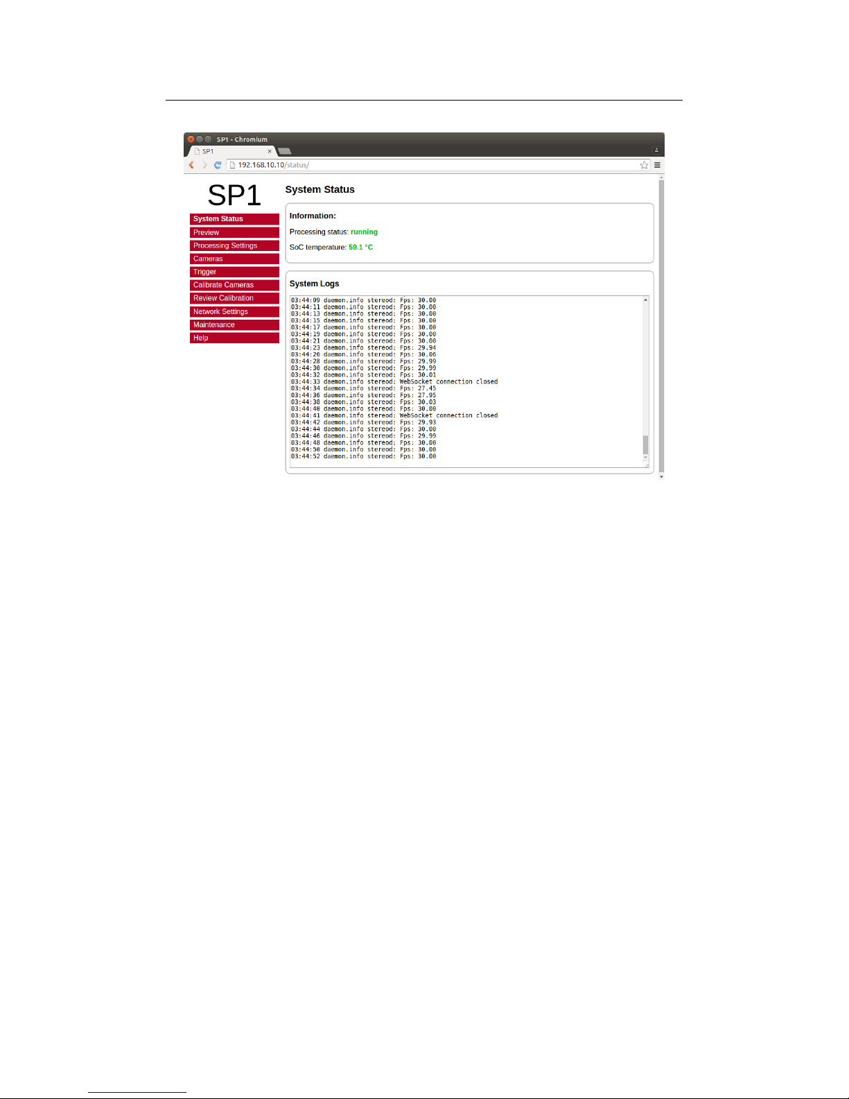
The first page that you will see when opening the web interface, is the system
status page that is shown in Figure 10. On this page you can find the following
information:
Processing status: Indicates whether the image processing sub-system has
been started. If this is not the case then there might be a problem
accessing the cameras, or another system error might have occurred.
Please consult the system logs in this case. The image processing subsystem will be started immediately once the cause of error has been
removed (such as connecting the cameras).
SOC temperature: The temperature of the central System-on-Chip (SoC)
that performs all processing tasks. The maximum allowed temperature
11
Page 13
8.2 Preview 8 CONFIGURATION
Figure 10: Screenshot of configuration status page.
is at 70◦C. A green-orange-red color-coding is applied to signal good,
alarming and critical temperatures.
System logs: List of system log messages sorted by time. In regular operation
you will find information on the current system performance. In case of
errors, the system logs will contain a corresponding error message.
8.2 Preview
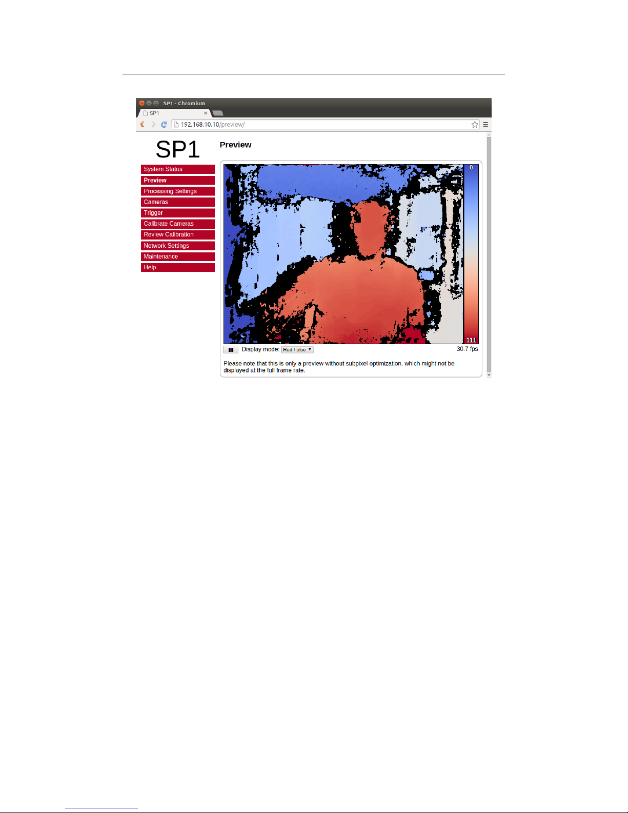
The preview page, which is shown in Figure 11, provides a live preview of the
currently computed disparity map. Please make sure that your network connection supports the high bandwidth that is required for streaming video data
(see Section 6.1). For using the preview page you require a direct connection
to the SP1. An in-between proxy server or a router that performs network
address translation (NAT) cannot be used.
When opening the preview page, the SP1 stops transferring image data to
any other host. The transfer is continued as soon as the browser window is
closed, the user presses the pause button below the preview area, or if the user
navigates to a different page. Only one open instance of the preview page,
or any other page that is streaming video data to the browser, is allowed at
a time. If attempted to open more than once, only one instance will receive
data.
The preview that is displayed in the browser does not reflect the full qual-
12
Page 14
8.2 Preview 8 CONFIGURATION
Figure 11: Screenshot of configuration preview page.
ity of the computed disparity map. In particular, sub-pixel accuracy is not
available, and your browser might not be able to display the disparity map at
the full camera frame rate. To receive a full-quality preview, please use the
SpCom sample application, which is described in Section 10.
Different color-coding schemes can be selected through the drop-down list
below the preview area. A color scale is shown to the right, which provides
information on the mapping between colors and disparity values. The possible
color schemes are:
Red / blue: A gradient from red to blue, with red hues corresponding to
high disparities and blue hues corresponding to low disparities. Invalid
disparities are depicted in black.
Rainbow: A rainbow color scheme with low wavelengths corresponding to
high disparities and high wavelengths corresponding to low disparities.
Invalid disparities are depicted in grey.
Raw data: The raw disparity data without color-coding. The pixel inten-
sity matches the integer component of the measured disparity. Invalid
disparities are displayed in light gray.
13
Page 15
8.3 Processing Settings 8 CONFIGURATION
Figure 12: Screenshot of configuration page for processing settings.
8.3 Processing Settings
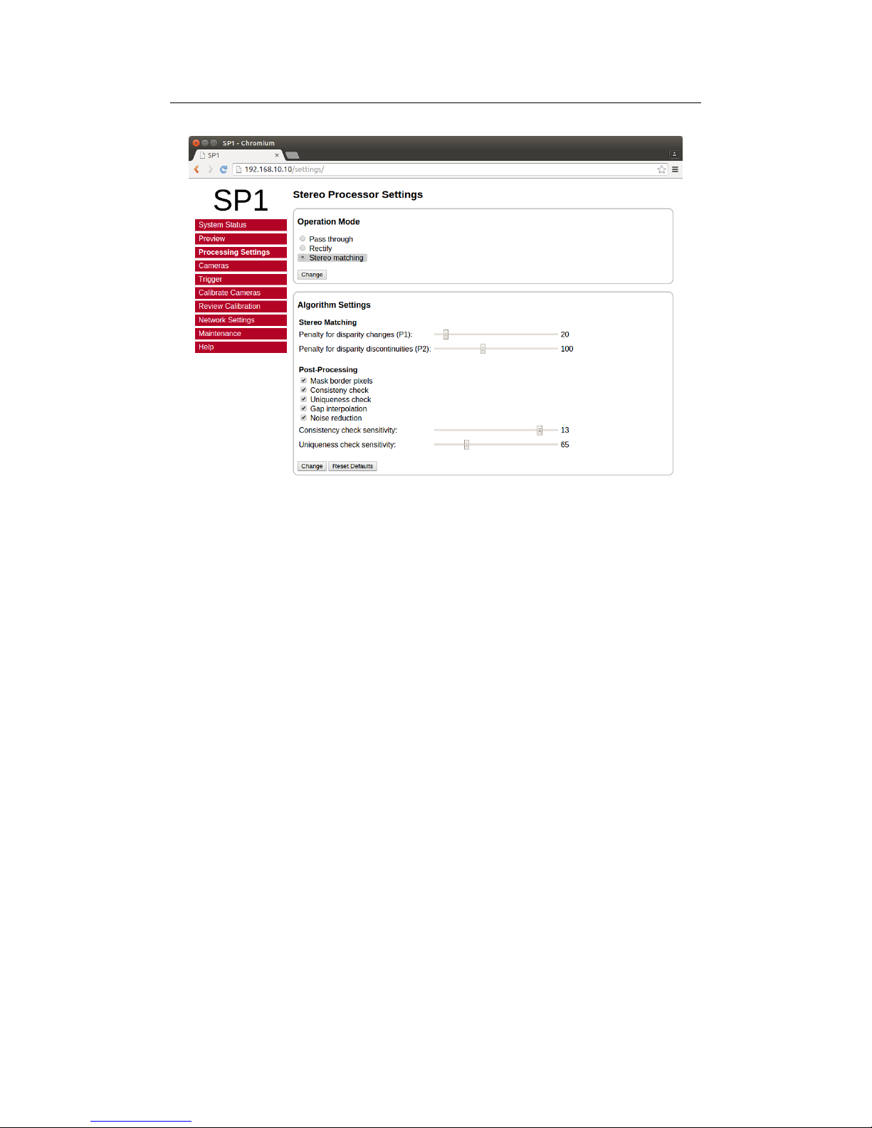
The major processing parameters can be changed on the processing settings
page, which is shown in Figure 12. The most relevant option is the operation
mode, which can be set to one of the following values:
Pass through: In this mode the SP1 forwards the imagery of the selected
cameras without modification. This mode is intended for verifying that
both cameras are functioning correctly.
Rectify: In this mode the SP1 transmits the rectified images of both cameras.
This mode is intended for verifying the correctness of image rectification.
Stereo matching: In this mode the SP1 performs stereo matching. It trans-
mits the rectified image of the left camera and the left camera disparity
map.
Please note that for pass through and rectify mode, the the right
image pixels have to be divided by 16, in order to receive the correct
intensities. This is due to the fact that the right image is always transmitted
with a bit depth of 12 bits.
If the operation mode is set to stereo matching, then the behavior of the
image processing algorithms can be controlled through the algorithm settings.
These settings include the following stereo matching parameters:
14
Page 16

8.4 Cameras 8 CONFIGURATION
Penalty for disparity changes (P1): A penalty that is applied for gradu-
ally changing disparities. A large value causes gradual disparity changes
to occur less frequently, while a small value causes gradual changes to
occur more frequently. This value has to be smaller than P2.
Penalty for disparity discontinuities (P2): A penalty that is applied to
abruptly changing disparities. A large value causes disparity discontinuities to occur less frequently, while a small value causes discontinuities
to occur more frequently. This value has to be greater than P1.
The SP1 implements several methods for post-processing of the computed
disparity map. Each post-processing method can be activated or deactivated
individually. The available methods are:
Mask border pixels: If enabled, this option marks all disparities that are
close to the border of the visible image area as invalid, as they have a high
likelihood of being wrong. This also includes all pixels for which no actual
image data is available due to the image rectification (see Section 7.1).
Consistency check: If enabled, stereo matching is performed in both match-
ing directions, left-to-right and right-to-left. Pixels for which there is no
consistent disparity are marked as invalid. The sensitivity of the consistency check can be controlled through the consistency check sensitivity
slider.
Uniqueness check: If enabled, pixels are marked as invalid if there is no suf-
ficiently unique solution (i.e. the cost function does not have a global
minimum that is significantly lower than all other local minima). The
sensitivity of the uniqueness check can be controlled through the unique-
ness check sensitivity slider.
Gap interpolation: If enabled, then small patches of invalid disparities, which
are caused by either the consistency or the uniqueness check, are filled
through interpolation.
Noise reduction: If enabled, an image filter is applied to the disparity map,
which reduces noise and removes outliers.
8.4 Cameras
8.4.1 Camera Selection
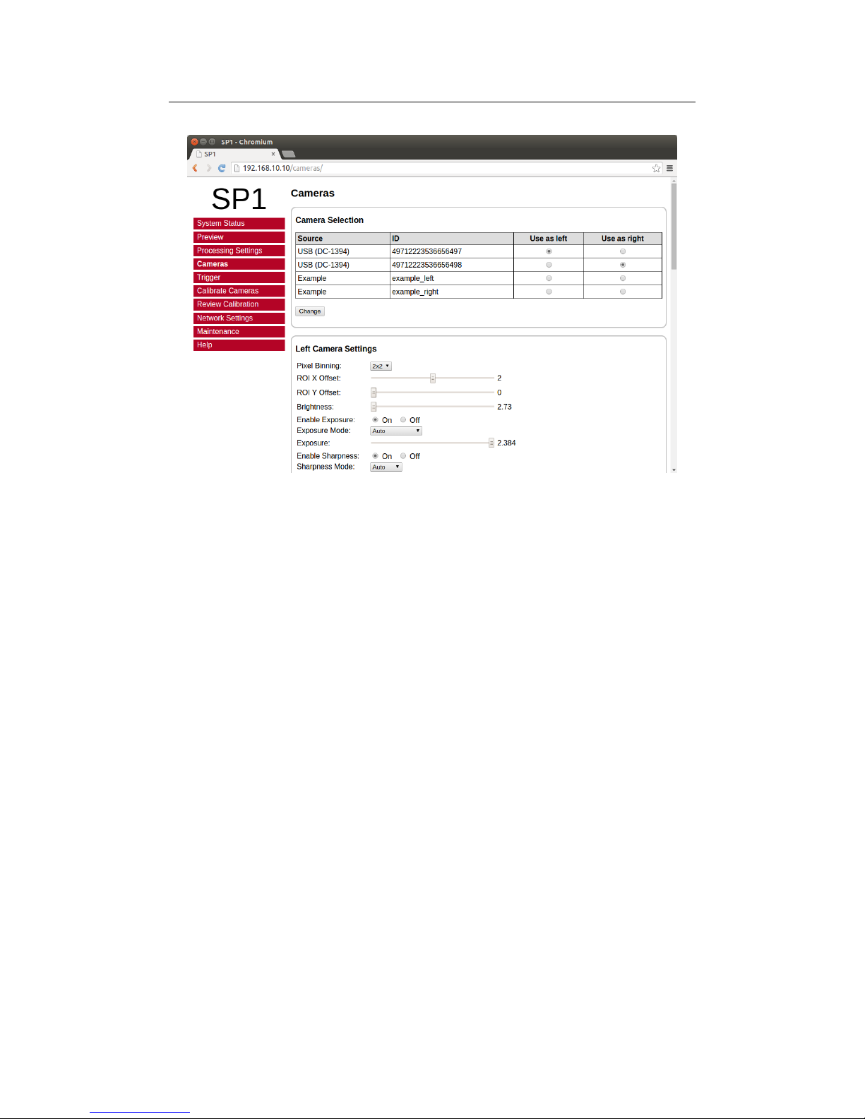
The cameras page that is shown in Figure 13 allows for the selection of a
desired camera pair and the adjustment of their respective parameters. All
detected cameras are listed in the camera selection list. A source is listed
for each camera, which identifies the utilized camera driver. To allow for an
easy evaluation, the SP1 ships with an example stereo sequence on its internal
15
Page 17
8.4 Cameras 8 CONFIGURATION
Figure 13: Screenshot of configuration page for camera settings.
memory. This example sequence appears as a virtual left and virtual right
camera.
To choose a particular camera, you have to tick either the use as left or
use as right radio button, for selecting the camera as the left or right camera
of the stereo pair. Please note that cameras of different sources cannot be
used together. If one of the virtual example cameras is selected, the example
sequence is replayed in an infinite loop. Due to speed limitations of the internal
memory, the example sequence will not be played at the full frame rate during
the first loop.
8.4.2 Camera Settings
After selecting a camera pair, camera specific settings can be adjusted in the
left camera settings and right camera settings area. The available settings depend on your camera model. Please refer to your camera documentation for
details. Some of the more advanced settings of your camera might not be
available. In this case please use the software provided by the camera manufacturer to adjust the desired settings and safe the new camera configuration
to the cameras’ internal memory.
By pressing the reset camera defaults button you can reset the camera’s
settings to the default configuration. This is usually the configuration that
has been written to the camera’s internal memory though the manufacturer
software. If the reset button is pressed, all configuration changes that have not
yet been confirmed through the change button will be reverted.
16
Page 18

8.4 Cameras 8 CONFIGURATION
The SP1 offers the functionality to synchronize parameters that are otherwise automatically adjusted by each camera. For example, each camera might
control its shutter time through an auto shutter algorithm. The SP1 can synchronize such auto-adjusted parameters by setting the parameters of the left
camera to always match the respective parameters of the right camera.
If this functionality is desired, the mode for the particular feature has to
be set to synchronize to left camera in the right camera settings, and to auto
in the left camera settings. In this case, the SP1 will query the settings of the
left camera and adjust the right camera’s settings accordingly.
8.4.3 Recommended Settings for Point Grey Cameras
When using Point Grey USB cameras we recommend that you use the following
settings:
• Enable external trigger and select the desired trigger source.
• If the cameras are connected to the SP1’s trigger port, set the trigger
polarity to active high. Otherwise set the polarity according to your
trigger source.
• Set the trigger mode to 0 or 14. Always use mode 14 if the internal
camera frame rate is not significantly higher than the trigger frequency.
• For the left camera, set the mode of exposure, sharpness, shutter and
gain to auto.
• For the right camera, set the mode of exposure, sharpness, shutter and
gain to synchronize to left camera.
8.4.4 Recommended Settings for IDS Cameras
When using cameras from IDS Imaging we recommend that you use the following settings:
• If the cameras shall be triggered by the SP1 trigger output:
– Due to voltage levels, the SP1 trigger output needs to be connected
to a camera GPIO pin, rather than the trigger input.
– The connected GPIO pin needs to be selected as trigger source.
– The trigger mode shall be set to hardware trigger, rising edge.
• Set the camera frame rate to at least twice the trigger frequency.
• For the left camera, set the mode of gain, exposure / shutter and black
level to auto.
• For the right camera, set the mode of gain, exposure / shutter and black
level to synchronize to left camera.
17
Page 19
8.5 Trigger 8 CONFIGURATION
Figure 14: Screenshot of configuration page for trigger settings.
8.5 Trigger
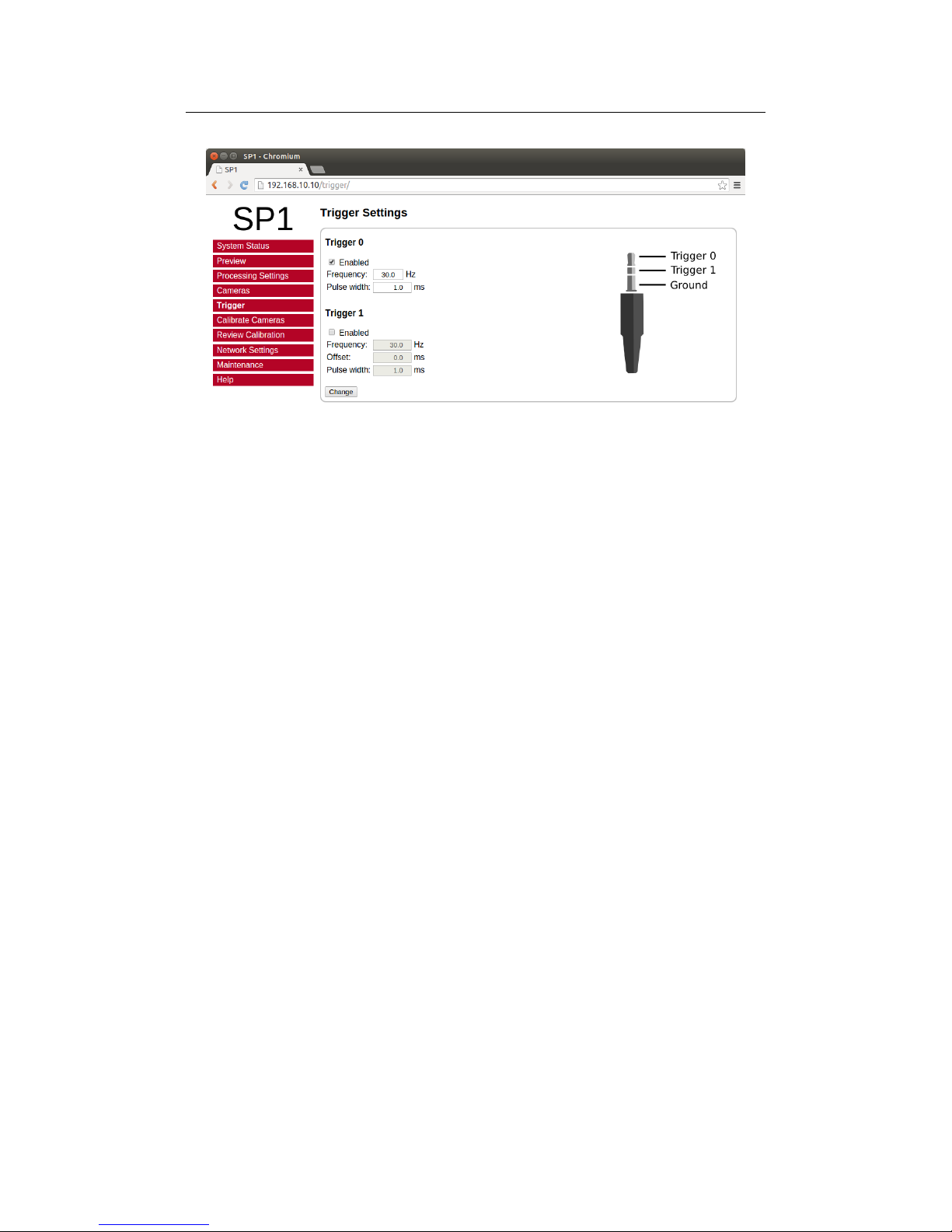
The trigger page that is shown in Figure 14 allows for adjusting the external
trigger settings. As described in Section 6.4, the SP1 features a trigger port
that provides access to up to two trigger signals. The two trigger signals,
trigger 0 and trigger 1, can be enabled or disabled by selecting the respective
check boxes.
For trigger 0 it is possible to select a frequency between 6 and 50 Hz and
an arbitrary pulse width in milliseconds. The polarity of the generated trigger
signal is active high.
The signal trigger 1 can only be enabled if trigger 0 is also enabled. The
frequency is forced to the same value as trigger 0. However, it is possible to
specify a time offset, which is the delay from a rising edge of trigger 0 to a
rising edge of trigger 1. Furthermore, trigger 1 can have a pulse width that
differs from trigger 0.
8.6 Camera Calibration
8.6.1 Calibration Board
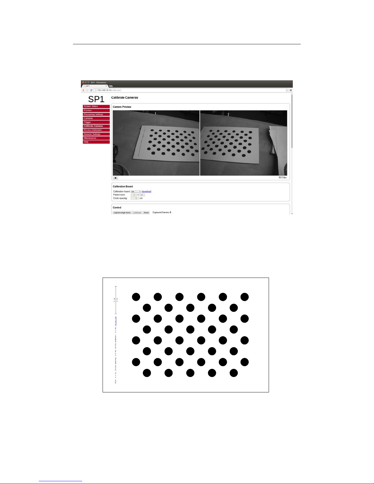
The calibrate cameras page, which is shown in Figure 15, enables the calibration
of the stereo camera pair. You require a calibration board, which is a flat panel
with a visible calibration pattern on one side. The pattern that is used by the
SP1 consists of an asymmetric grid of black circles on a white background, as
shown in Figure 16.
The pattern can be downloaded directly from the calibration page. Simply
select the desired paper size in the calibration board drop-down list, and click
the download link. Even if you already have a calibration board, make sure
to always select the correct board size before starting the calibration process.
Otherwise the calibration results cannot be used for 3D reconstruction with a
18
Page 20
8.6 Camera Calibration 8 CONFIGURATION
Figure 15: Screenshot of configuration page for camera calibration.
Size: 4 x 11; Circle spacing: 2.0 cm; Circle diameter: 1.5 cm;
5 cm
2 in
nerian.com
Figure 16: Calibration board used by SP1.
19
Page 21

8.6 Camera Calibration 8 CONFIGURATION
correct metric scale (see Section 7.2).
Should you require a calibration board with a custom size, then you can
select custom from the calibration board drop-down list. This allows you to
enter the calibration board details manually. The first dimension of the pattern
size is the number of circles in one grid column. This number must be equal
for all columns of the circles grid.
The number of circles per row is allowed to vary by 1 between odd and
even rows. The second dimension is thus the sum of circles in two consecutive
rows. All downloadable default calibration patterns have a size of 4 × 11.
The final parameter that you have to enter when using a custom calibration
board is the circle spacing. This is the distance between the centers of two
neighboring circles. The distance must be equal in horizontal and vertical
direction for all circles.
8.6.2 Recording Calibration Frames
Once the calibration board settings have been set, you can begin recording
calibration frames. A live preview of both cameras is displayed in the camera
preview area. Make sure that the calibration board is fully visible in both
camera images and then press the capture single frame button in the control
section. Repeat this process several times while moving either the camera or
the calibration board.
The calibration board must be recorded at several different positions and
orientations. You should also vary the distance of the board to the cameras and
make sure that you cover most of the cameras’ field of view. When recording
the calibration frames it is important that both cameras are synchronized.
The more frames you record, the more accurate the computed calibration
will be. However, more frames also cause the computation of the calibration
parameters to take longer. The SP1 supports the recording of up to 40 calibration frames.
The recording of calibration frames can be simplified by activating the auto
capture mode. In this mode, a new calibration frame is recorded in fix capture
intervals. You can enter the desired interval in the auto capture section and
then press the start auto capture button. If desired, an audible sound can
be played to signal the countdown and the recording of a new frame. Auto
capture mode can be stopped by pressing the stop auto capture button.
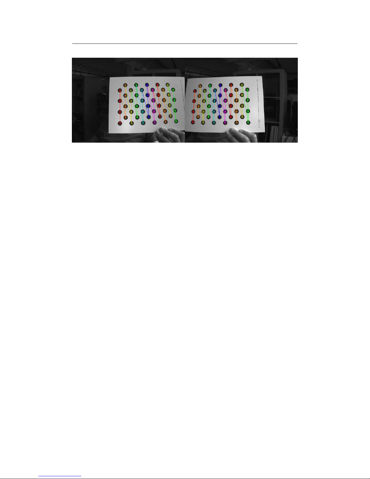
A small preview of each captured calibration frame is added to the captured
frames section. The frames are overlaid with the detected positions of the
calibration board circles. You can click any of the preview images to see the
calibration frame at its full resolution. An example for a calibration frame with
a correctly detected calibration board is shown in Figure 17. If the calibration
board was not detected correctly or if you are unhappy with the quality of a
calibration frame, then you can delete it by clicking on the ×-symbol.
20
Page 22
8.7 Reviewing Calibration Results 8 CONFIGURATION
Figure 17: Example calibration frame with detected calibration board.
8.6.3 Performing Calibration
Once you have recorded a sufficient number of calibration frames, you can
initiate the calibration process by pressing the calibrate button in the control
section. The time required for camera calibration depends on the number of
calibration frames that you have recorded. Calibration will usually take several
minutes to complete. If calibration is successful then you are immediately
redirected to the review calibration page.
Calibration will fail if the computed vertical or horizontal pixel displacement exceeds the allowed range of [−31, +31] for any image point. The most
likely causes for a failed calibration are:
• Insufficient number of calibration frames.
• Improperly aligned cameras. See Section 6.3.
• Lenses with strong geometric distortions.
• Lenses with unequal focal lengths.
• Not synchronized cameras.
• Frames with misdetected calibration board.
Should calibration fail, then please resolve the cause of error and repeat the
calibration process. If the cause of error is one or more erroneous calibration
frames, then you can delete those frame and re-press the calibrate button.
Likewise, in case of too few calibration frames, you can record additional frames
and restart the calibration process.
8.7 Reviewing Calibration Results
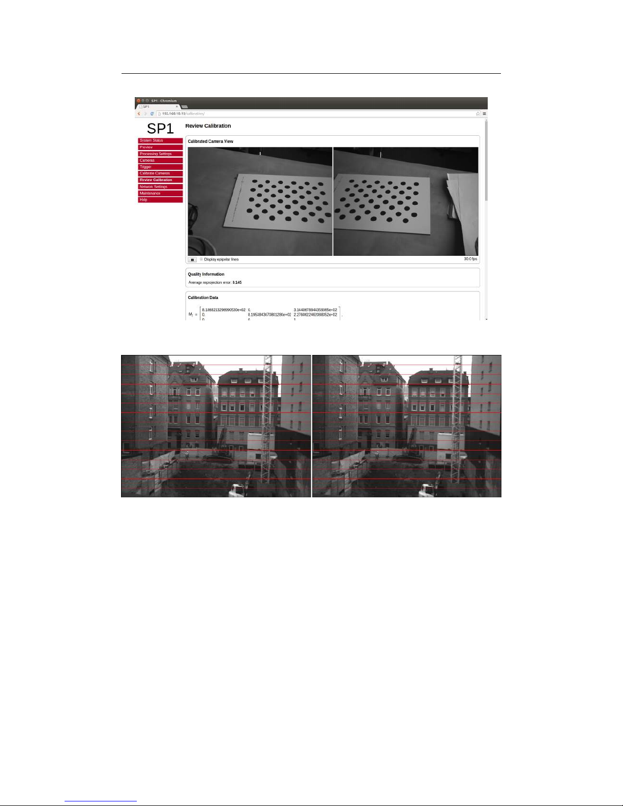
Once calibration has been performed you can inspect the calibration results
on the review calibration page. On the top of this page you see a live preview
21
Page 23
8.7 Reviewing Calibration Results 8 CONFIGURATION
Figure 18: Screenshot of configuration page for reviewing camera calibration.
Figure 19: Example for evaluating vertical image coordinates.
of both cameras, which have been rectified with the current calibration parameters. Please make sure that corresponding points in the images of both
cameras have an identical vertical coordinate.
By activating the display epipolar lines option, you can overlay a set of
horizontal lines on both camera images. This allows for an easy evaluation of
whether the equal vertical coordinates criterion is met. An example for a left
and right input image with overlaid epipolar lines is shown in Figure 19.
In the quality information section you can find the average reprojection
error. This is a measure for the quality of your camera calibration, with lower
values indicating a better calibration result. Please make sure that the average
reprojection error is well below 1 pixel.
All computed calibration parameters are displayed in the calibration data
22
Page 24

8.7 Reviewing Calibration Results 8 CONFIGURATION
section. These parameters are:
M1and M2: camera matrices for the left and right camera.
D1and D2: distortion coefficients for the left and right camera.
R1and R2: rotation matrix for the rotation between the original and rectified
camera images.
P1and P2: projection matrices in the new (rectified) coordinate systems.
Q: the disparity-to-depth mapping matrix. See Section 7.2 for its use.
T: translation vector between the coordinate systems of both cameras.
R: rotation matrix between the coordinate systems of the left and right cam-
era.
The camera matrices M1and M2are structured as follows:
Mi=
fx0 c
x
0 fyc
y
0 0 1
, (1)
where fxand fyare the lenses’ focal lengths in horizontal and vertical
direction (measured in pixels), and cxand cyare the image coordinates of the
projection center.
The distortion coefficient vectors D1and D2have the following structure:
Di=
k1k2p1p2k
3
, (2)
where k1, k2and k3are radial distortion coefficients, and p1and p2are
tangential distortion coefficients.
You can download all calibration information as a machine-readable YAML
file, by clicking the download link at the bottom of the calibration data section.
This allows you to easily import the calibration data into your own applications. Furthermore, you can save the calibration data to your PC and reload it
at a later point, by using the upload calibration data section. This allows you
to switch between different cameras or optics without repeating the calibration
process.
You can also perform a reset of the calibration data by pressing the reset
calibration button. In this case, image rectification will be disabled, and the
unmodified image data will be passed on to the stereo matching algorithm.
Use this option when selecting the already rectified virtual example camera,
as explained in Section 8.4.
23
Page 25
8.8 Network Settings 8 CONFIGURATION
Figure 20: Screenshot of configuration page for network settings.
8.8 Network Settings
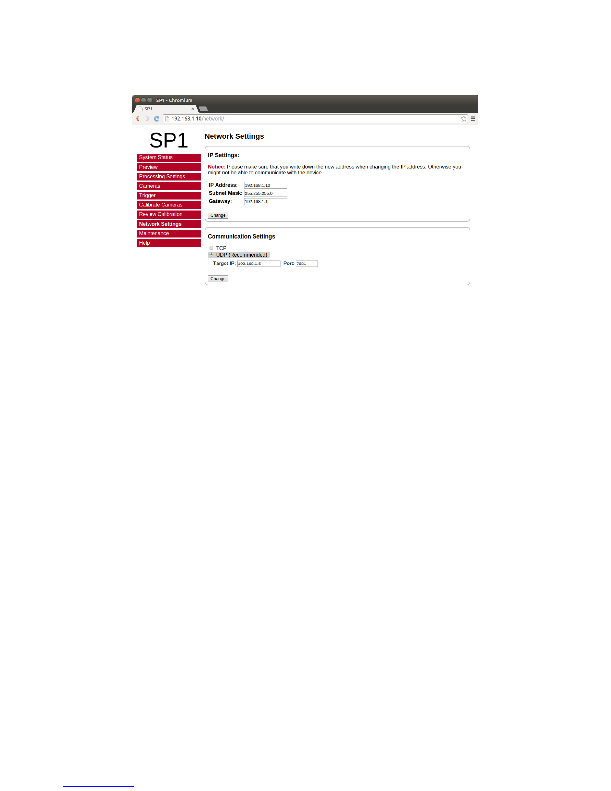
The network settings page, which is displayed in Figure 20, is used for configuring all network related parameters. In the IP settings section, you can
specify an IP address, subnet mask and gateway address. When changing the
IP settings, please make sure that your computer is in the same subnet, or that
there exists a gateway router through which data can be transferred between
both subnets. Otherwise you will not be able to access the SP1.
In the communication settings section, you can choose the underlying net-
work protocol that shall be used for delivering the computation results to the
client computer. The possible options are TCP and UDP. Due to the highbandwidth real time data, we recommend using UDP.
If TCP is selected, the SP1 will open up the server port 7681 and wait
for a client computer to connect before transmitting data. Because UDP is a
connection-less protocol, data transmission starts instantly if UDP is selected.
In UDP mode you thus have to specify the IP address and port number of the
client computer. It is possible to enter a multicast address here, if you want
the data to be received by multiple hosts or processes.
8.9 Maintenance
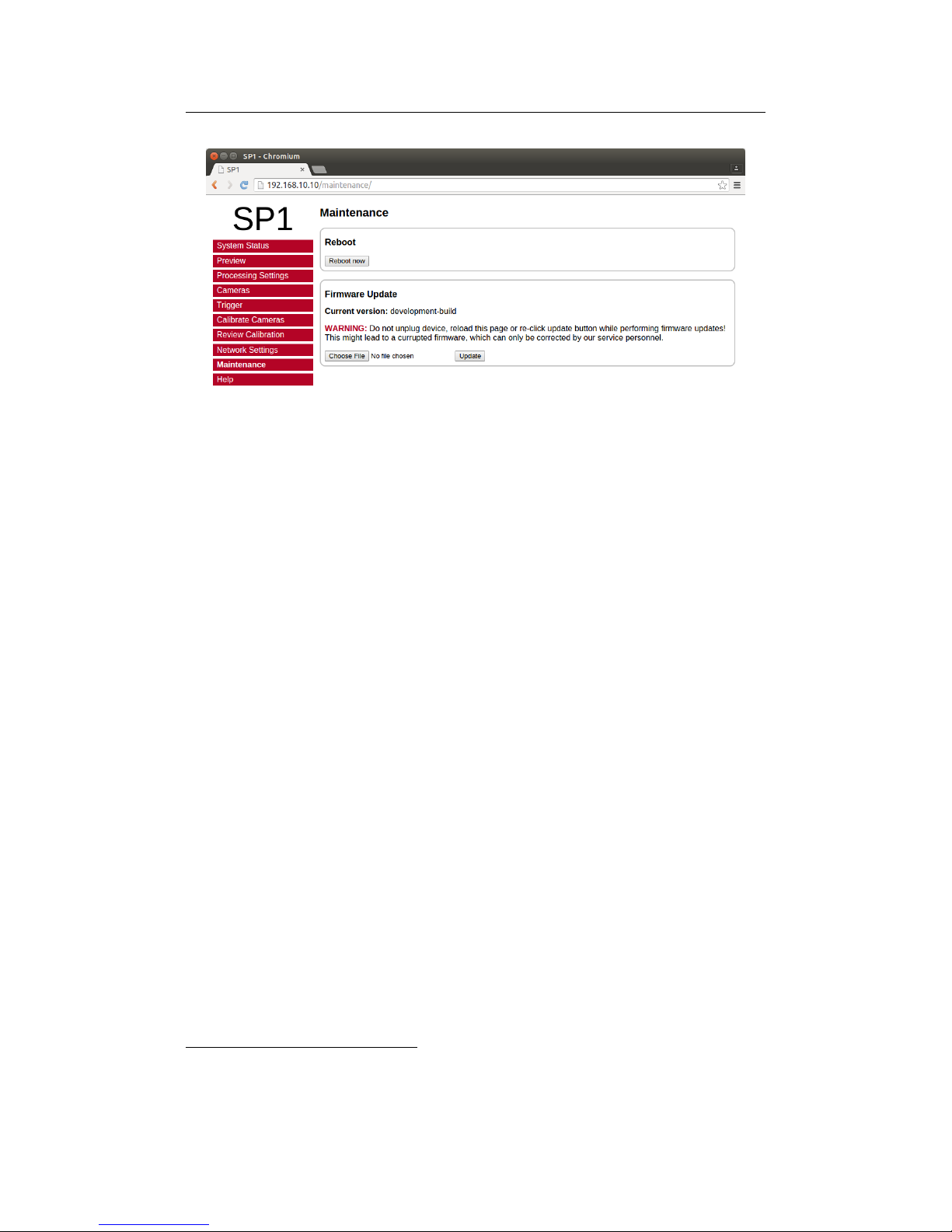
The maintenance page, which is shown in Figure 21, allows you to trigger
a reboot of the SP1. This can be done by pressing the reboot now button.
Perform this step if the SP1 has stopped functioning correctly. When a reboot
is triggered it will take several seconds before the device will be reachable
again.
The maintenance page further allows you to perform firmware updates. Use
24
Page 26
9 API USAGE INFORMATION
Figure 21: Screenshot of configuration maintenance page.
this functionality only for firmware files that have officially been released by
Nerian Vision Technologies. To perform a firmware update, select the desired
firmware file and press the update button. The update process will take several
seconds. Do not unplug the device, reload the maintenance page or re-click
the update button while performing firmware updates. Otherwise, this might
lead to a corrupted firmware.
9 API Usage Information
9.1 General Information
The cross-platform libvisiontransfer C++ API is available for interfacing custom software with the SP1. For windows, a binary version of the library is
available that can be used with Microsoft Visual Studio 2013 and 2015. For
Linux and Mac OSX, please compile the library from the available source code
package. The API can be downloaded from the product website2.
The libvisiontransfer API provides functionally for receiving the processing
results of the SP1 over a computer network. Furthermore, the API also allows
for the transmission of image data. It can thus be used for emulating an SP1
when performing systems development.
The transmitted processing results always consist of two images. Usually
these are the rectified left camera image and the computed left camera disparity
map. If configured, however, the SP1 can also provide the raw camera images
or the rectified images of both cameras (see Section 8.4).
The first transmitted image always has a bit-depth of 8 bits and the second
image has a bit depth of 12 bits. Inside the library, the second image is inflated
to 16 bits to allow for more efficient processing.
2
http://nerian.com/products/sp1-stereo-vision/
25
Page 27

9.2 ImageTransfer Example 9 API USAGE INFORMATION
The API provides three classes that can be used for receiving and transmitting image data:
• ImageProtocol is the most low-level interface. This class allows for the
encoding and decoding of images to / from network messages. You will
have to handle all network communication yourself.
• ImageTransfer opens up a network socket for sending and receiving
network messages. This class is single-threaded and will thus block when
receiving or transmitting data.
• AsyncTransfer allows for the asynchronous reception or transmission of
network messages. This class creates one or more threads that handle
all network communication.
Detailed information on the usage of each class can be found in the available
API documentation.
9.2 ImageTransfer Example
An example for using the class ImageTransfer to receive processing results
over the network, and writing them to image files is shown below. This source
code file is part of the API source code package. Please refer to the API documentation for further information on using ImageTransfer.
#i n c l u d e <v i s i o n t r a n s f e r / i m a g e t r ansf e r . h>
#i n c l u d e <iost r e am>
#i n c l u d e <fstr e am>
#i n c l u d e <s t d i o . h>
#i f d e f _WIN32
#i n c l u d e <win s ock 2 . h>
#e l s e
#i n c l u d e <arp a / i n e t . h>
#e n d if
#i f d e f _MSC_VER
// Visual s t u d i o d oes no t come w ith s n p r i n t f
#d e f i n e s n p r i n t f _snpr intf_ s
#e n d if
i n t main ( ) {
// C r eate an image t r a n s f e r objec t that re c e i v e s d ata f rom
// t h e SP1 on t h e d e f a ul t port u s i ng UDP
Imag e Tran s f er i mageT r a n sfer ( Image T rans f e r : : UDP_CLIENT, NULL,
" 7681" ) ;
// Rec e i v e 100 i mag es
f o r ( i n t i =0; i <10 0; i ++) {
26
Page 28

9.2 ImageTransfer Example 9 API USAGE INFORMATION
std : : cout << " R eceiving␣im age ␣ " << i << std : : e ndl ;
// A l t e r na t i n g l y re c e i v e the f i r s t and se c ond image
f o r ( i n t imageNumber = 0; imageNumber <=1; imageNumber++) {
// Rec e i v e image
i n t widt h , h eight , r o w S t ride ;
Imag e P roto c ol : : ImageFormat for mat ;
unsi g n ed c har∗ pixe l D a t a = NULL;
while ( p i x e l D ata == NULL) {
pixelDa t a = imageT r a nsfer . r e ceiveImage ( imageNumber ,
wi dth , h e ight , r owSt r i de , f orma t ) ;
}
// C r eate PGM f i l e
char file N a me [ 1 0 0 ] ;
s n p r i n t f ( fil eNam e , s i z e o f ( f i leNam e ) , " ima ge%03d_%d. pgm" , i ,
imageNumber ) ;
std : : f s tream st rm ( file Name , s td : : i o s : : out ) ;
// Write PGM h e ader
i n t maxVal , b y tesP i x e l ;
i f ( f orma t == Ima g e Prot o col : : FORMAT_8_BIT) {
maxVal = 2 5 5 ;
b y t e s P i x e l = 1;
} e l s e { // 12 b i t
maxVal = 4 0 9 5 ;
b y t e s P i x e l = 2;
}
strm << "P5␣" << width << "␣" << h e i g h t << "␣ " << maxVal
<< s t d : : e n d l ;
// Write imag e dat a
f o r ( i n t y = 0 ; y < height ; y++) {
f o r ( i n t x = 0 ; x < w idt h ; x++) {
unsi g n ed c har∗ p i x e l = &pixelD a t a [
y∗ rowStri d e + x∗ b y t e s P i x e l ] ;
i f ( b y t e s P i x e l == 2) {
// Swap endianes s
∗ r e inte r p r e t _ c a s t <u n sign e d sh o r t ∗ >( p i x e l )
= hto ns (∗ r e int e r p r e t _ c a s t <u n signe d s h o r t ∗ >( p i x e l ) ) ;
}
strm . w r i t e ( r e i n t e r p ret_ c a s t <cha r ∗ >( p i x e l ) , b y t e s P i x e l ) ;
}
}
}
}
return 0 ;
}
27
Page 29

9.3 AsyncTransfer Example 9 API USAGE INFORMATION
9.3 AsyncTransfer Example
An example for using the class AsyncTransfer to receive processing results
over the network, and writing them to image files is shown below. This source
code file is part of the API source code package. Please refer to the API doc-
umentation for further information on using AsyncTransfer.
#i n c l u d e <v i s i o n t r a n s f e r / a s y n c t r a n s f e r . h>
#i n c l u d e <iost r e am>
#i n c l u d e <fstr e am>
#i n c l u d e <s t d i o . h>
#i f d e f _WIN32
#i n c l u d e <win s ock 2 . h>
#e l s e
#i n c l u d e <arp a / i n e t . h>
#e n d if
#i f d e f _MSC_VER
// Visual s t u d i o d oes no t come w ith s n p r i n t f
#d e f i n e s n p r i n t f _snpr intf_ s
#e n d if
i n t main ( ) {
// C r eate an as ync t r a n s f e r objec t that r e c e i v e s d ata from
// t h e SP1 on t h e d e f a ul t port u s i ng UDP
Asyn c Tran s fer asyncTran s f e r ( I mage T ransf e r : : UDP_CLIENT, NULL,
" 7681" ) ;
// Rec e i v e 100 i mag es
f o r ( i n t i =0; i <10 0; i ++) {
std : : cout << " R eceiving␣im age ␣ " << i << std : : e ndl ;
// A l t e r na t i n g l y re c e i v e the f i r s t and se c ond image
f o r ( i n t imageNumber = 0; imageNumber <=1; imageNumber++) {
i n t widt h , h eight , r o w S t ride ;
Imag e P roto c ol : : ImageFormat for mat ;
unsi g n ed c har∗ pixe l D a t a = NULL;
// Keep on tryi n g to r e c e i v e an ima ge u n t i l s u c c e s s f u l
while ( p i x e l D ata == NULL) {
pixelDa t a = a s y ncTransfe r . c o l l e c t R e c e i v e d I m a g e (
imageNumber , wi dth , h eight , r o wStri d e , fo rma t ,
0 . 1 /∗ time o ut ∗ / ) ;
}
// C r eate PGM f i l e
char file N a me [ 1 0 0 ] ;
s n p r i n t f ( fil eNam e , s i z e o f ( f i leNam e ) , " ima ge%03d_%d. pgm" , i ,
imageNumber ) ;
std : : f s tream st rm ( file Name , s td : : i o s : : out ) ;
28
Page 30

9.4 3D Reconstruction 10 SPCOM SAMPLE APPLICATION
// Write PGM h e ader
i n t maxVal , b y tesP i x e l ;
i f ( f orma t == Ima g e Prot o col : : FORMAT_8_BIT) {
maxVal = 2 5 5 ;
b y t e s P i x e l = 1;
} e l s e { // 12 b i t
maxVal = 4 0 9 5 ;
b y t e s P i x e l = 2;
}
strm << "P5␣" << width << "␣" << h e i g h t << "␣ " << maxVal
<< s t d : : e n d l ;
// Write imag e dat a
f o r ( i n t y = 0 ; y < height ; y++) {
f o r ( i n t x = 0 ; x < w idt h ; x++) {
unsi g n ed c har∗ p i x e l = &pixelD a t a [
y∗ rowStri d e + x∗ b y t e s P i x e l ] ;
i f ( b y t e s P i x e l == 2) {
// Swap endianes s
∗ r e inte r p r e t _ c a s t <u n sign e d sh o r t ∗ >( p i x e l )
= hto ns (∗ r e int e r p r e t _ c a s t <u n signe d s h o r t ∗ >( p i x e l ) ) ;
}
strm . w r i t e ( r e i n t e r p ret_ c a s t <cha r ∗ >( p i x e l ) , b y t e s P i x e l ) ;
}
}
}
}
return 0 ;
}
9.4 3D Reconstruction
As described in Section 7.2, the disparity map can be transformed into a set of
3D points. This requires knowledge of the disparity-to-depth mapping matrix
Q, which can be obtained from the review calibration page of the web interface
(see Section 8.7).
An optimized implementation of the required transformation, which uses
SSE or AVX instructions, is provided by the API through the class Reconstruct3D.
This class converts a disparity map to a map of 3D point coordinates. Please
see the API documentation for details on using this class.
10 SpCom Sample Application
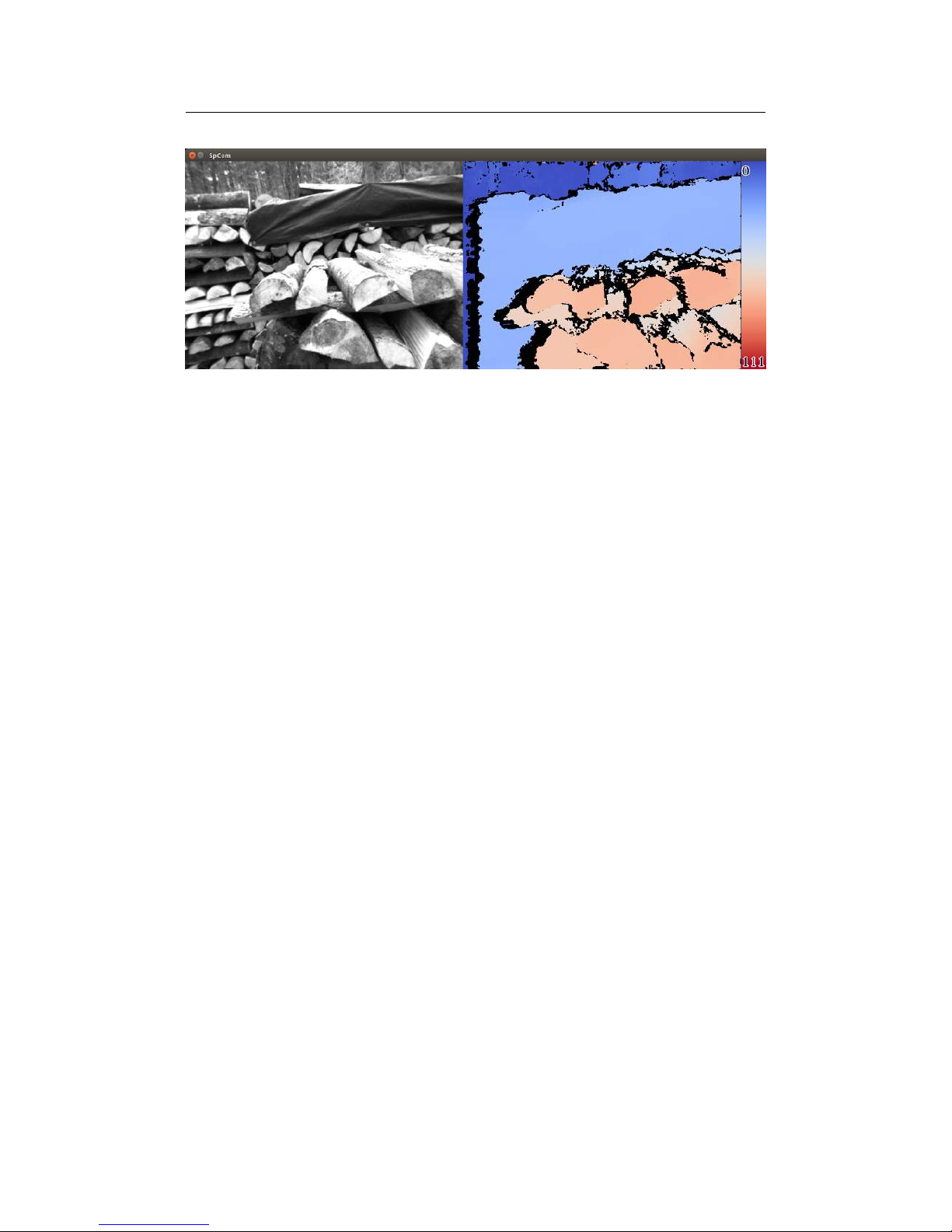
The downloadable source code or binary version of the libvisiontransfer API
also include the SpCom sample application, which is shown in Figure 22. When
compiling this application yourself, please make sure that you have the libraries
OpenCV and libSDL installed.
29
Page 31
10 SPCOM SAMPLE APPLICATION
Figure 22: Screenshot of SpCom sample application.
SpCom provides the following features:
• Receive and display images and disparity maps from SP1.
• Perform color-coding of disparity maps.
• Write received data to image files.
• Transmit a set of images over the network and thus emulate the SP1.
SpCom should be run from a terminal in order to supply command line
arguments and to view the printed status messages. If the graphical mode
is not disabled, then SpCom opens up a window for displaying the received
images. The currently displayed images can be written to files by pressing
the space key. When pressing the enter key, all received images are written to
files up until enter is re-pressed. The created image files will be located in the
current working directory.
SpCom can be controlled with the following command line options:
30
Page 32

12 WARRANTY INFORMATION
-c Color code the disparity map.
-s directory Server mode (emulating SP1). The images in the given di-
rectory will be read and sent out over the network.
-n Non-graphical mode. No display window will be opened.
-f number Limits the frame rate to the given value. This option can be
used in server mode for controlling the replay speed.
-w directory Immediately start writing all received images to the given
directory.
-h hostname Use the given hostname for communication. This option
should be specified when connecting to the SP1 through TCP,
or when operating in server mode while using the UDP protocol.
-p port Use the given port number for communication. The default
port number is 7681.
-t Use TCP instead of UDP as the underlying network protocol.
-r Output the right image (usually the disparity map) as raw
12-bit image without bit-depth conversion.
-i 0/1 Only display image 0 (left) or 1 (right).
11 Support
If you require support or if you have other inquiries that are related to this
product, please contact:
Dr. Konstantin Schauwecker
Nerian Vision Technologies
Gotenstr. 9
70771 Leinfelden-Echterdingen
Germany
Phone: +49-1577-1956789
E-mail: [email protected]
Website: http://nerian.com
12 Warranty Information
The device is provided with a 2 year warranty according to German federal
law (BGB). Warranty is lost if:
• the housing is opened by others than official Nerian Vision Technologies
service staff.
• the firmware is modified or replaced, except for official firmware updates.
In case of warranty please contact our support staff.
31
Page 33

13 OPEN SOURCE INFORMATION
13 Open Source Information
The firmware of the SP1 contains code from the open source libraries and
applications listed in Table 1. Source code for these software components and
the wording of the respective software licenses can be obtained from the open
source information website3. Some of these components may contain code from
other open source projects, which have not been listed here. For a definitive
list, please consult the respective source packages.
Table 1: Open source components.
Name
Version License(s)
busybox 1.22.1 GNU GPL 2.0
dropbear 2014.63 MIT License
BSD License
OpenSSH License
Sourcery CodeBench
2014.11-30 GNU GPL 2.0
Lite for Xilinx GNU GPL 3.0
Cortex-A9 Mentor Graphics License
GNU/Linux BSD / Various
libffi 3.1 MIT
glib 2.40 GPL 2.0
libdc1394 2.2.3 (patched) GNU LGPL 2.1
libusb 1.0.18 GNU LGPL 2.1
libwebsockets 1.3 GNU LGPL 2.1
libxml 2-2.9.1 MIT License
linux 3.18.0-xilinx GNU GPL 2.0
monit 5.13 GNU GPL 3.0
opencv 2.4.9 BSD License
libpng License
JasPer License 2.0
openssl 1.0.2c OpenSSL License
zlib 1.2.8 Zlib License
The following individuals have requested to be named as author or co-
author of one of the included open source projects:
Google Inc., The Android Open Source Project, Red Hat Incorporated, University of California, Berkeley, David M. Gay, Christopher G. Demetriou, Royal Institute of Technology, Alexey Zelkin, Andrey A. Chernov, FreeBSD, S.L. Moshier, Citrus Project, Todd C.
Miller, DJ Delorie, Intel Corporation, Henry Spencer, Mike Barcroft, Konstantin Chuguev,
Artem Bityuckiy, IBM, Sony, Toshiba, Alex Tatmanjants, M. Warner Losh, Andrey A.
Chernov, Daniel Eischen, Jon Beniston, ARM Ltd, CodeSourcery Inc, MIPS Technologies
3
http://nerian.com/products/sp1-stereo-vision/open-source/
32
Page 34

13 OPEN SOURCE INFORMATION
Inc, Addison-Wesley, Advanced Micro Devices Inc., Alexander Chemeris, Alexander Neundorf, Alexandre Benoit, Alexandre Julliard, Andreas Dilger, Andrei Alexandrescu, Andrey
Kamaev, Annecy le Vieux and GIPSA Lab, Argus Corp, Arren Glover, AWare Systems, Baptiste Coudurier, Chih-Chung Chang, Chih-Jen Lin, Christopher Diggins, Clement Boesch,
David G. Lowe, Edward Rosten„ Enrico Scholz, EPFL Signal processing laboratory 2, Ethan
Rublee, ETH Zurich Autonomous Systems Lab (ASL), Fabrice Bellard, Farhad Dadgostar,
Frank D. Cringle, Glenn Randers-Pehrson, Google Inc., Greg Ward Larson, Group 42 Inc.,
Guy Eric Schalnat, Image Power Inc., Industrial Light & Magic, Institute Of Software Chinese Academy Of Science, Intel Corporation, Ivan Kalvachev, James Almer, Javier Sánchez
Pérez, Jean-loup Gailly, Joris Van Damme Joseph O’Rourke, Jostein Austvik Jacobsen,
Justin Ruggles, Ken Turkowski, Kevlin Henney, GIPSA French Labs, LISTIC Lab, Liu
Liu, Maarten Lankhorst, Makoto Matsumoto, Mans Rullgard, Marius Muja, Mark Adler,
Martin Storsjo, Michael David Adams, Michael Niedermayer, Microsoft Corporation, Multicoreware Inc., Nicolas George, Nils Hasler, NVIDIA Corporation, OpenCV Foundation,
Pablo Aguilar, Peter Ross, PhaseSpace Inc., Philipp Wagner, Pixar Animation Studios,
Reimar Döffinger, Rob Hess, Ryan Martell, Sam Leffler, Samuel Pitoiset, Silicon Graphics
Inc., Simon Perreault, Smartjog S.A.S, Splitted-Desktop Systems, Takuji Nishimura, The
Khronos Group Inc., The Regents of the University of California, the Sphinx team, The University of British Columbia, the Wine project, Thomas G. Lane, University of Augsburg,
Weta Digital Ltd, William Lucas, Willow Garage Inc., Xavier Delacour, Yossi Rubner
If you believe that your name should be included in this list, then please
let us know.
33
Page 35

Revision History 13 OPEN SOURCE INFORMATION
Revision History
Revision Date Author(s) Description
v1.0 August 28, 2015 KS List of compatible cameras, infor-
mation on IDS cameras, software
download link, extended open
source information, general improvements.
v0.1 July 30, 2015 KS Initial revision
34
 Loading...