

Page 1

NCT® 99M
NCT® 2000M
Controls for Milling Machines and Machining Centers
Programmer's Manual
Page 2

Manufactured by NCT Automation kft.
H1148 Budapest Fogarasi út 7
: Address: H1631 Bp. pf.: 26
F Phone: (+36 1) 467 63 00
F Fax:(+36 1) 363 6605
E-mail: [email protected]
Home Page: www.nct.hu
Page 3
Contents
1 Introduction ..............................................................9
1.1 The Part Program ......................................................9
Word ...............................................................9
Address Chain .........................................................9
Block ..............................................................10
Program Number and Program Name ......................................10
Beginning of Program, End of Program ......................................10
Program Format in the Memory ...........................................10
Program Format in Communications with External Devices .......................10
Main Program and Sub-program ..........................................10
DNC Channel ........................................................11
1.2 Fundamental Terms ....................................................12
2 Controlled Axes .........................................................17
2.1 Names of axes .......................................................17
2.2 Unit and Increment System of Axes ........................................17
3 Preparatory Functions (G codes) ............................................19
4 The Interpolation ........................................................22
4.1 Positioning (G00) .....................................................22
4.2 Linear Interpolation (G01) ...............................................22
4.3 Circular and Spiral Interpolation (G02, G03) .................................24
4.4 Helical Interpolation (G02, G03) ..........................................27
4.5 Equal Lead Thread Cutting (G33) .........................................29
4.6 Polar Coordinate Interpolation (G12.1, G13.1) ...............................31
4.7 Cylindrical Interpolation (G7.1) ...........................................35
5 The Coordinate Data .....................................................38
5.1 Absolute and Incremental Programming (G90, G91), Operator I ..................38
5.2 Polar Coordinates Data Command (G15, G16) ...............................38
5.3 Inch/Metric Conversion (G20, G21) .......................................40
5.4 Specification and Value Range of Coordinate Data ............................40
5.5 Rotary Axis Roll-over ..................................................41
6 The Feed ...............................................................45
6.1 Feed in rapid travers ...................................................45
6.2 Cutting Feed Rate .....................................................45
6.2.1 Feed per Minute (G94) and Feed per Revolution (G95) ....................46
6.2.2 Clamping the Cutting Feed ..........................................47
6.3 Automatic Acceleration/Deceleration .......................................48
6.4 Feed Control Functions .................................................49
6.4.1 Exact Stop (G09) .................................................49
3
Page 4

6.4.2 Exact Stop Mode (G61) ........................................... 49
6.4.3 Continuous Cutting Mode (G64) ..................................... 50
6.4.4 Override and Stop Inhibit (Tapping) Mode (G63) ........................ 50
6.4.5 Automatic Corner Override (G62) .................................... 50
6.4.6 Internal Circular Cutting Override ..................................... 51
7 The Dwell (G04) ......................................................... 52
8 The Reference Point ..................................................... 53
8.1 Automatic Reference Point Return (G28) ................................... 53
8.2 Automatic return to reference points 2nd, 3rd, 4th (G30) ....................... 54
8.3 Automatic Return from the Reference Point (G29) ............................. 54
9 Coordinate Systems, Plane Selection ........................................ 56
9.1 The Machine Coordinate System ......................................... 56
9.1.1 Setting the Machine Coordinate system ................................ 57
9.1.2 Positioning in the Machine Coordinate System (G53) ...................... 57
9.2 Work Coordinate Systems .............................................. 57
9.2.1 Setting the Work Coordinate Systems ................................. 57
9.2.2 Selecting the Work Coordinate System ................................ 58
9.2.3 Programmed Setting of the Work Zero Point Offset ....................... 59
9.2.4 Creating a New Work Coordinate System (G92) ......................... 59
9.3 Local Coordinate System ............................................... 60
9.4 Plane Selection (G17, G18, G19) ......................................... 62
10 The Spindle Function .................................................... 64
10.1 Spindle Speed Command (code S) ....................................... 64
10.2 Programming of Constant Surface Speed Control ............................ 64
10.2.1Constant Surface Speed Control Command (G96, G97) ................... 65
10.2.2 Constant Surface Speed Clamp (G92) ................................ 65
10.2.3 Selecting an Axis for Constant Surface Speed Control .................... 66
10.3 Spindle Position Feedback ............................................. 66
10.4 Oriented Spindle Stop ................................................ 66
10.5 Spindle Positioning (Indexing) ........................................... 67
10.6 Spindle Speed Fluctuation Detection (G25, G26) ............................ 67
11 Tool Function .......................................................... 70
11.1 Tool Select Command (Code T) ......................................... 70
11.2 Program Format for Tool Number Programming ............................. 70
12 Miscellaneous and Auxiliary Functions ..................................... 72
12.1 Miscellaneous Functions (Codes M) ...................................... 72
12.2 Auxiliary Function (Codes A, B, C) ...................................... 73
12.3 Sequence of Execution of Various Functions ................................ 73
13 Part Program Configuration............................................... 74
4
Page 5
13.1 Sequence Number (Address N) .........................................74
13.2 Conditional Block Skip ................................................74
13.3 Main Program and Sub-program .........................................74
13.3.1 Calling the Sub-program ...........................................74
13.3.2 Return from a Sub-program ........................................75
13.3.3 Jump within the Main Program ......................................77
14 The Tool Compensation ..................................................78
14.1 Referring to Tool Compensation Values (H and D) ...........................78
14.2 Modification of Tool Compensation Values from the Program (G10) ..............79
14.3 Tool Length Compensation (G43, G44, G49) ...............................80
14.4 Tool Offset (G45...G48) ...............................................81
14.5 Cutter Compensation (G38, G39, G40, G41, G42) ...........................85
14.5.1 Start up of Cutter Compensation .....................................88
14.5.2 Rules of Cutter Compensation in Offset Mode ...........................92
14.5.3 Canceling of Offset Mode ..........................................95
14.5.4 Change of Offset Direction While in the Offset Mode .....................98
14.5.5 Programming Vector Hold (G38) ...................................100
14.5.6 Programming Corner Arcs (G39) ...................................100
14.5.7 General Information on the Application of Cutter Compensation ............102
14.5.8 Interferences in Cutter Compensation ................................107
14.6 Three-dimensional Tool Offset (G41, G42) ................................112
14.6.1 Programming the Three-dimensional Tool Offset (G40, G41, G42) ..........112
14.6.2 The Three-dimensional Offset Vector ................................113
15 Special Transformations .................................................115
15.1 Coordinate System Rotation (G68, G69) ..................................115
15.2 Scaling (G50, G51) ..................................................116
15.3 Programmable Mirror Image (G50.1, G51.1) ..............................117
15.4 Rules of Programming Special Transformations .............................118
16 Automatic Geometric Calculations ........................................120
16.1 Programming Chamfer and Corner Round .................................120
16.2 Specifying Straight Line with Angle ......................................121
16.3 Intersection Calculations in the Selected Plane ..............................123
16.3.1 Linear-linear Intersection ..........................................123
16.3.2 Linear-circular Intersection ........................................125
16.3.3 Circular-linear Intersection ........................................127
16.3.4 Circular-circular Intersection .......................................129
16.3.5 Chaining of Intersection Calculations .................................131
17 Canned Cycles for Drilling ...............................................132
17.1 Detailed Description of Canned Cycles ...................................138
17.1.1 High Speed Peck Drilling Cycle (G73) ...............................138
17.1.2 Counter Tapping Cycle (G74) ......................................139
17.1.3 Fine Boring Cycle (G76) ..........................................140
5
Page 6
17.1.4 Canned Cycle Cancel (G80) ...................................... 141
17.1.5 Drilling, Spot Boring Cycle (G81) ................................... 141
17.1.6 Drilling, Counter Boring Cycle (G82) ................................ 142
17.1.7 Peck Drilling Cycle (G83) ........................................ 143
17.1.8 Tapping Cycle (G84) ............................................ 144
17.1.9 Rigid (Clockwise and Counter-clockwise) Tap Cycles (G84.2, G84.3) ....... 145
17.1.10 Boring Cycle (G85) ............................................ 148
17.1.11 Boring Cycle Tool Retraction with Rapid Traverse (G86) ................ 149
17.1.12 Boring Cycle/Back Boring Cycle (G87) ............................. 150
17.1.13 Boring Cycle (Manual Operation on the Bottom Point) (G88) ............. 152
17.1.14 Boring Cycle (Dwell on the Bottom Point, Retraction with Feed) (G89) ..... 153
17.2 Notes to the use of canned cycles ....................................... 153
18 Measurement Functions ................................................ 155
18.1 Skip Function (G31) ................................................. 155
18.2 Automatic Tool Length Measurement (G37) ............................... 156
19 Safety Functions ....................................................... 158
19.1 Programmable Stroke Check (G22, G23) ................................. 158
19.2 Parametric Overtravel Positions ........................................ 159
19.3 Stroke Check Before Movement ....................................... 160
20 Custom Macro ........................................................ 161
20.1 The Simple Macro Call (G65) ......................................... 161
20.2 The Modal Macro Call ............................................... 162
20.2.1 Macro Modal Call in Every Motion Command (G66) .................... 162
20.2.2 Macro Modal Call From Each Block (G66.1) ......................... 163
20.3 Custom Macro Call Using G Code ...................................... 164
20.4 Custom Macro Call Using M Code ..................................... 165
20.5 Subprogram Call with M Code ......................................... 165
20.6 Subprogram Call with T Code ......................................... 166
20.7 Subprogram Call with S Code ......................................... 166
20.8 Subprogram Call with A, B, C Codes .................................... 166
20.9 Differences Between the Call of a Sub-Program and the Call of a Macro .......... 167
20.9.1 Multiple Calls .................................................. 167
20.10 Format of Custom Macro Body ....................................... 169
20.11 Variables of the Programming Language ................................. 169
20.11.1 Identification of a Variable ....................................... 169
20.11.2 Referring to a variable .......................................... 169
20.11.3 Vacant Variables .............................................. 170
20.11.4 Numerical Format of Variables .................................... 170
20.12 Types of Variables ................................................. 171
20.12.1 Local Variables ............................................... 171
20.12.2 Common Variables ............................................ 171
20.12.3 System Variables .............................................. 172
20.13 Instructions of the Programming Language ................................ 180
6
Page 7

20.13.1 Definition, Substitution ..........................................180
20.13.2 Arithmetic Operations and Functions ................................181
20.13.3 Logical Operations .............................................184
20.13.4 Unconditional Divergence ........................................184
20.13.5 Conditional Divergence ..........................................185
20.13.6 Conditional Instruction ..........................................185
20.13.7 Iteration .....................................................185
20.13.8 Data Output Commands .........................................188
20.14 NC and Macro Instructions ...........................................191
20.15 Execution of NC and Macro Instructions in Time ...........................191
20.16 Displaying Macros and Sub-programs in Automatic Mode ....................192
20.17 Using the STOP Button While a Macro Instruction is Being Executed ............192
20.18 Pocket-milling Macro Cycle ..........................................193
Notes ..................................................................197
Index in Alphabetical Order ................................................198
July 2, 2002
7
Page 8

© Copyright NCT July 2, 2002
The Publisher reserves all rights for contents
of this Manual. No reprinting, even in
extracts, is permissible unless our written
consent is obtained.
The text of this Manual has been compiled
and checked with utmost care, yet we
assume no liability for possible errors or
spurious data and for consequential losses or
demages.
8
Page 9
1 Introduction
1 Introduction
1.1 The Part Program
The Part Program is a set of instructions that can be interpreted by the control system in order to
control the operation of the machine.
The Part Program consists of blocks which, in turn, comprise words.
Word: Address and Data
Each word is made up of two parts - an address and a data. The address has one or more
characters, the data is a numerical value (an integer or decimal value). Some addresses may be given
a sign or operator I.
Address Chain:
Address Meaning Value limits
O program number 0001 - 9999
/ optional block 1 - 9
N block number 1 - 99999
G preparatory function *
X, Y, Z, U, V ,W length coordinates I, -, *
A, B, C angular coordinates, length coordinates, auxiliary
functions
R circle radius, auxiliary data I, -, *
I, J, K circle center coordinates, auxiliary coordinate -, *
E auxiliary coordinate -, *
F feed rate *
S spindle speed *
M miscellaneous function 1 - 999
T tool number 1 - 9999
H, D number of length and radius compensation cell 1 - 99
L repetition number 1 - 9999
P auxiliary data, dwell time -, *
Q auxiliary data -, *
,C distance of chamfer -, *
,R radius of fillet -, *
,A angle of straight line -, *
( comment *
I, -, *
At an address marked with a * in the Value Limits column, the data may have a decimal value as
well.
At an address marked with I and -, an incremental operator or a sign can be assigned, respectively.
The positive sign + is not indicated and not stored.
9
Page 10

1 Introduction
Block
A block is made up of words.
The blocks are separated by characters s (Line Feed) in the memory. The use of a block number
is not mandatory in the blocks. To distinguish the end of block from the beginning of another block
on the screen, each new block begins in a new line, with a character > placed in front of it, in the
case of a block longer than a line, the words in each new line are begun with an indent of one
character.
Program Number and Program Name
The program number and the program name are used for the identification of a program. The use of
program number is mandatory that of a program name is not.
The address of a program number is O. It must be followed by exactly four digits.
The program name is any arbitrary character sequence (string) put between opening "(" and
closing brackets ")". It may have max. 16 characters.
The program number and the program name are separated by characters s (Line Feed) from the
other program blocks in the memory.
In the course of editing, the program number and the program name will be displayed invariably in
the first line.
There may be not two programs of a given program number in the backing store.
Beginning of Program, End of Program
Each program begins and ends with characters %. In the course of part program editing the
program-terminating character is placed invariably behind the last block in order to ensure that the
terminated locks will be preserved even in the event of a power failure during editing.
Program Format in the Memory
The program stored in the memory is a set of ASCII characters.
The format of the program is
%O1234(PROGRAM NAME)s/1N12345G1X0Y...sG2Z5...s....s
...s
...s
N1G40...M2s
%
In the above sequence of characters,
s is character "Line Feed",
% is the beginning (and end) of the program.
Program Format in Communications with External Devices
The above program is applicable also in communications with an external device.
Main Program and Sub-program
The part programs may be divided into two main groups -
main programs, and
subprograms.
The procedure of machining a part is described in the main program. If, in the course of machining
repeated patterns have to be machined at different places, it is not necessary to write those
program-sections over and over again in the main program, instead, a sub-program has to be
organized, which can be called from any place (even from another sub-program). The user can
10
Page 11
1 Introduction
return from the sub-program to the calling program.
DNC Channel
A program contained in an external unit (e.g., in a computer) can also be executed without storing it
in the control's memory. Now the control will read the program, instead of the memory, from the
external data medium through the RS232C interface. That link is referred to as "DNC channel". This
method is particularly useful for the execution of programs too large to be contained in the control's
memory.
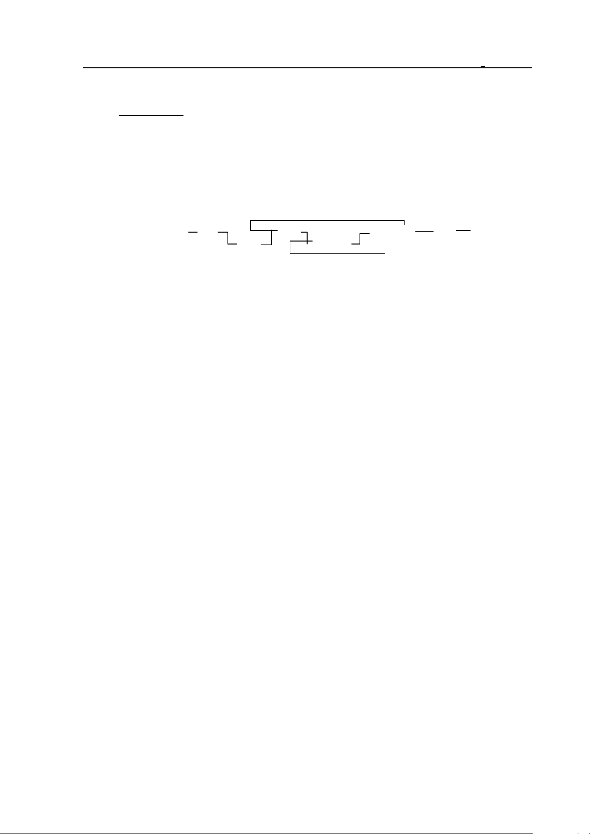
The DNC channel is a protocol-controlled data transfer channel as shown below.
Controller:
Equipment:
<
BEL > DC1 NAK/ACK DC3
ACK > BLOCK
<
The above mnemonics have the following meanings (and their ASCII codes):
BEL (7): The control requests the sender to establish the communication. The control issues
L again unless ACK is returned in a definite length of time.
ACK (6): acknowledgment.
NAK (21): Spurious data transfer (e.g. hardware trouble in the line or BCC error). The
transfer of BLOCK has to be repeated.
DC1 (17): Transfer of the next BLOCK has to be started.
DC3 (19): Interruption of communication.
BLOCK:
– Basically an NC block (including the terminating character s) and the checksum
thereof (BCC) stored in 7 bits as the last byte of the block (bit 7, the
uppermost one, of BCC is invariably 0). No SPACE (32) or some other
character of lower ASCII code may be contained in the block.
– EOF (26) (End Of File), a signal is transferred by the Equipment ("sender") to
interrupt the communication.
For the DNC mode, set the second physical channel (only that one is applicable as a DNC channel)
for 8-bit even-parity mode.
A main program executed from the DNC channel may have a linear sequence only. This does not
apply to subprogram or macro (if any have been called) however, they must be contained in the
memory of control. In the event of a departure from the linear sequence in the main program
(GOTO, DO WHILE), the control will return error message 3058 NOT IN DNC. If the control
detects a BLOCK error and returns NAK, the BLOCK has to be repeated.
11
Page 12
1 Introduction
1.2 Fundamental Terms
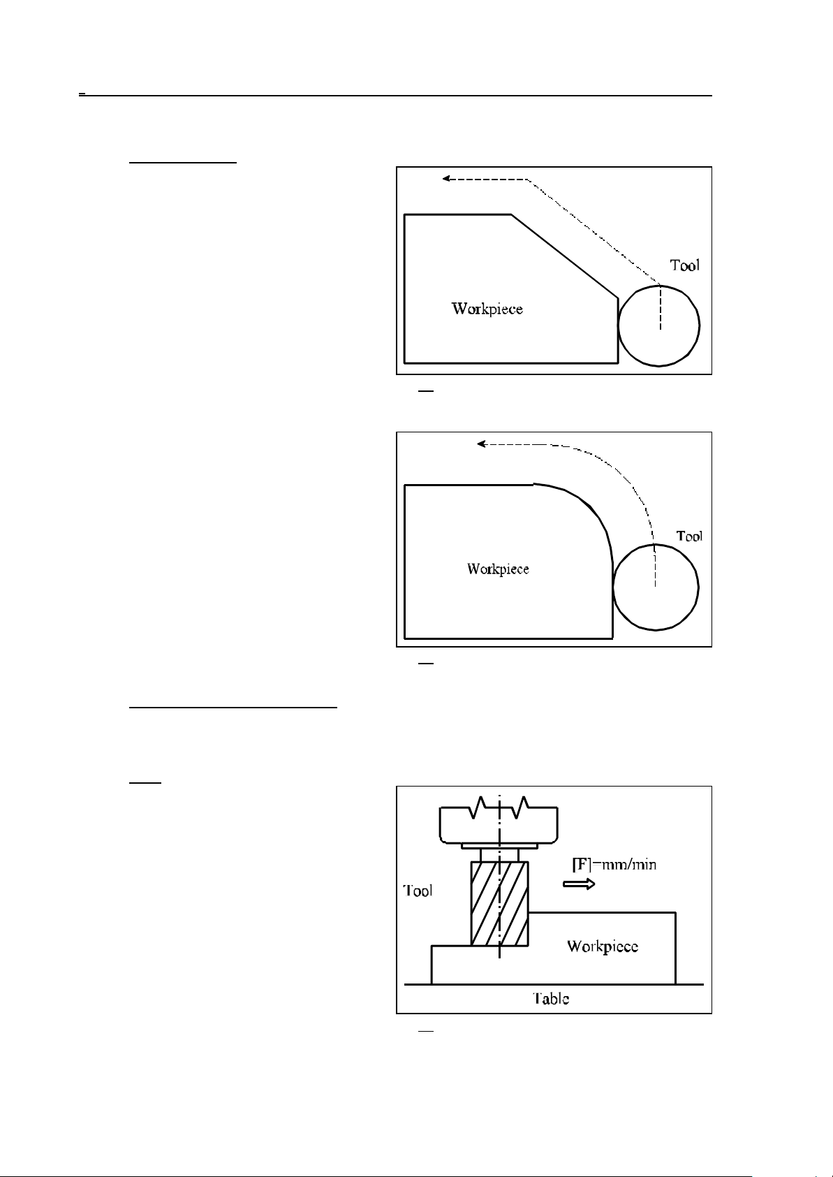
The Interpolation
The control system can move the tool along
straight lines and arcs in the course of machining. These activities will be hereafter referred
to as "interpolation".
Tool movement along a straight line:
program:
G01 Y__
X__ Y__
Tool movement along an arc:
program:
G03 X__ Y__ R__
Fig. 1.2-1
Although, in general, the table with the workpiece and not the tool moves, this description
will refer to the motion of the tool against the
workpiece.
Fig. 1.2-2
Preparatory Functions (G codes)
The type of activity to be performed by a block is described with the use of preparatory functions
(also referred to as G codes). E.g., code G01 introduces a linear interpolation.
Feed
The term "feed" refers to the speed of the tool
relative to the workpiece during the process of
cutting. The desired feed can be specified in the
program at address F and with a numerical
value. For example F150 means 150
mm/minute.
12
Fig. 1.2-3
Page 13
1 Introduction
Reference Point
The reference point is a fixed point on the machine-tool. After power-on of the machine, the slides
have to be moved to the reference point. Afterwards the control system will be able to interpret data
of absolute coordinates as well.
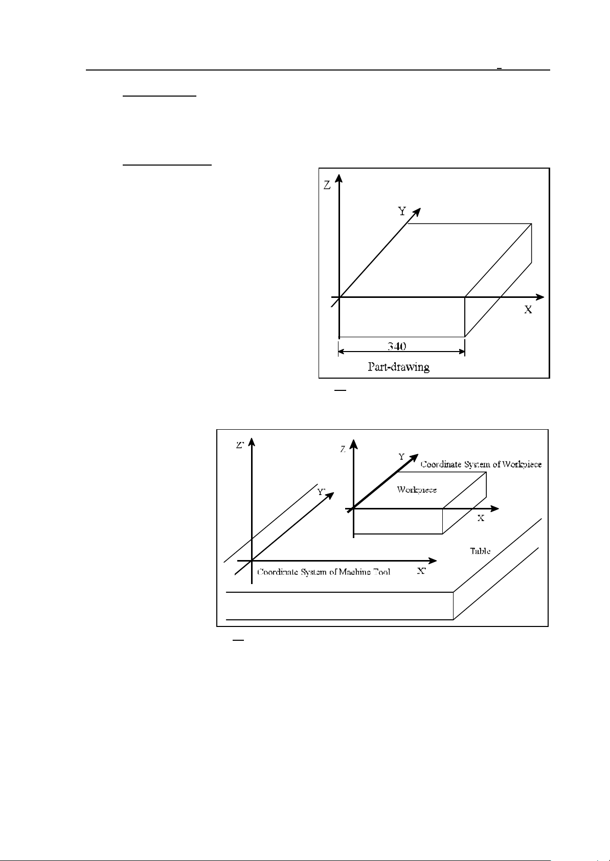
Coordinate System
The dimensions indicated in the part drawing
are measured from a given point of the part.
That point is the origin of the workpiece
coordinate system. Those dimensional data have
to be written at the coordinate address in the
part program. E.g., X340 means a point of
coordinate 340 mm in the coordinate system of
the workpiece.
Fig. 1.2-4
The coordinate system
specified in the control
system and in which the
control interprets the
positions, is different from
the coordinate system of
the workpiece. For the
control system to make a
correct workpiece, the
zero points of the two
coordinate systems have
to be set at the same
position. This can be
achieved, e.g., by moving
Fig. 1.2-5
the tool center to a point
of known position of the part and setting the coordinate system of the control to that value.
13
Page 14
1 Introduction
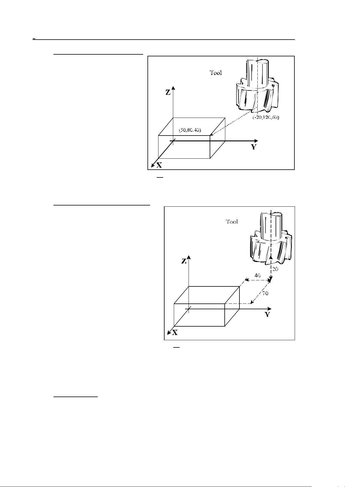
Absolute Coordinate Specification
When absolute coordinates are specified,
the tool travels a distance measured from
the origin of the coordinate system, i.e., to
a point whose position has been specified
by the coordinates.
The code of absolute data specification is
G90.
The block
G90 X50 Y80 Z40
will move the tool to a point of the above
position, irrespective of its position before
the command has been issued.
Fig. 1.2-6
Incremental Coordinate Specification
In the case of an incremental data specification,
the control system will interpret the coordinate
data in such a way that the tool will travel a
distance measured from its instantaneous
position.
The code of incremental data specification is
G91. Code G91 refers to all coordinate values.
The block
G91 X70 Y-40 Z-20
will move the tool over the above distance from
its previous position.
An incremental data may be defined to be
referred to a single coordinate as well. Standing
behind the address of the coordinate, character
I refers to the incremental specification of the
given coordinate value.
Fig. 1.2-7
In block
G90 XI-70 Y80 Z40
the data of X is interpreted as an incremental value, whereas data Y and Z are - for code G90 interpreted as absolute coordinates.
Modal Functions
Some codes are effective until another code or value is specified. These are modal codes. E.g., in
program detail
N15 G90 G1 X20 Y30 F180
N16 X30
N17 Y100
14
Page 15
1 Introduction
the code of G90 (absolute data specification) and the value of F (Feed), specified in block N15, will
be modal in blocks N16 and N17. Thus it is not necessary to specify those functions in each block
followed.
One-shot (Non-modal) Functions
Some codes or values are effective only in the block in which they are specified. These are one-shot
functions.
Spindle Speed Command
The spindle speed can be specified at address S. It is also termed as "S function". Instruction S1500
tells the spindle to rotate at a speed of 1500 rpm
Tool Function
In the course of machining different tools have to be employed for the various cutting operations.
The tools are differentiated by numbers. Reference can be made to the tools with code T.
Instruction T25 in the program means that tool No. 25 has to be changed. The tool change can be
carried out manually or automatically, depending on the design of the machine.
Miscellaneous Functions
A number of switching operations have to be carried out in the course of machining. For example,
starting the spindle, turning on the coolant. Those operations can be performed with M
(miscellaneous) functions. E.g., in the series of instructions
M3 M8
M3 means “rotate the spindle clockwise”, M8 means "turn on the coolant".
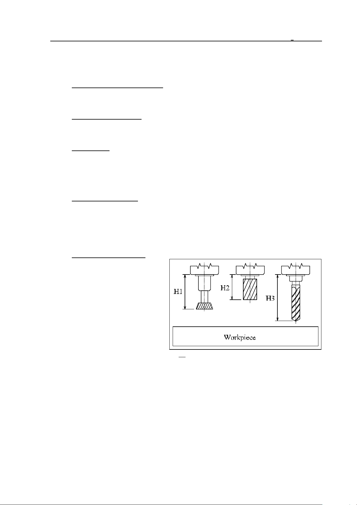
Tool Length Compensation
In the course of machining, tools of
different length are employed for the
various operations. On the other hand, a
given operation also has to be performed
with tools of different lengths in series
production (e.g., when the tool breaks).
In order to make the motions described in
the part program independent of the
length of the tool, the various tool lengths
must be set in control system. If the
program is intended to move the tip of the
Fig. 1.2-8
tool to the specified point, the value of the
particular length data has to be called. This is feasible at address H. E.g., instruction H1 refers to
length data No.1. Henceforth the control will move the tip of the tool to the specified point. That
procedure is referred to as setting “tool length compensation" mode.
15
Page 16
1 Introduction
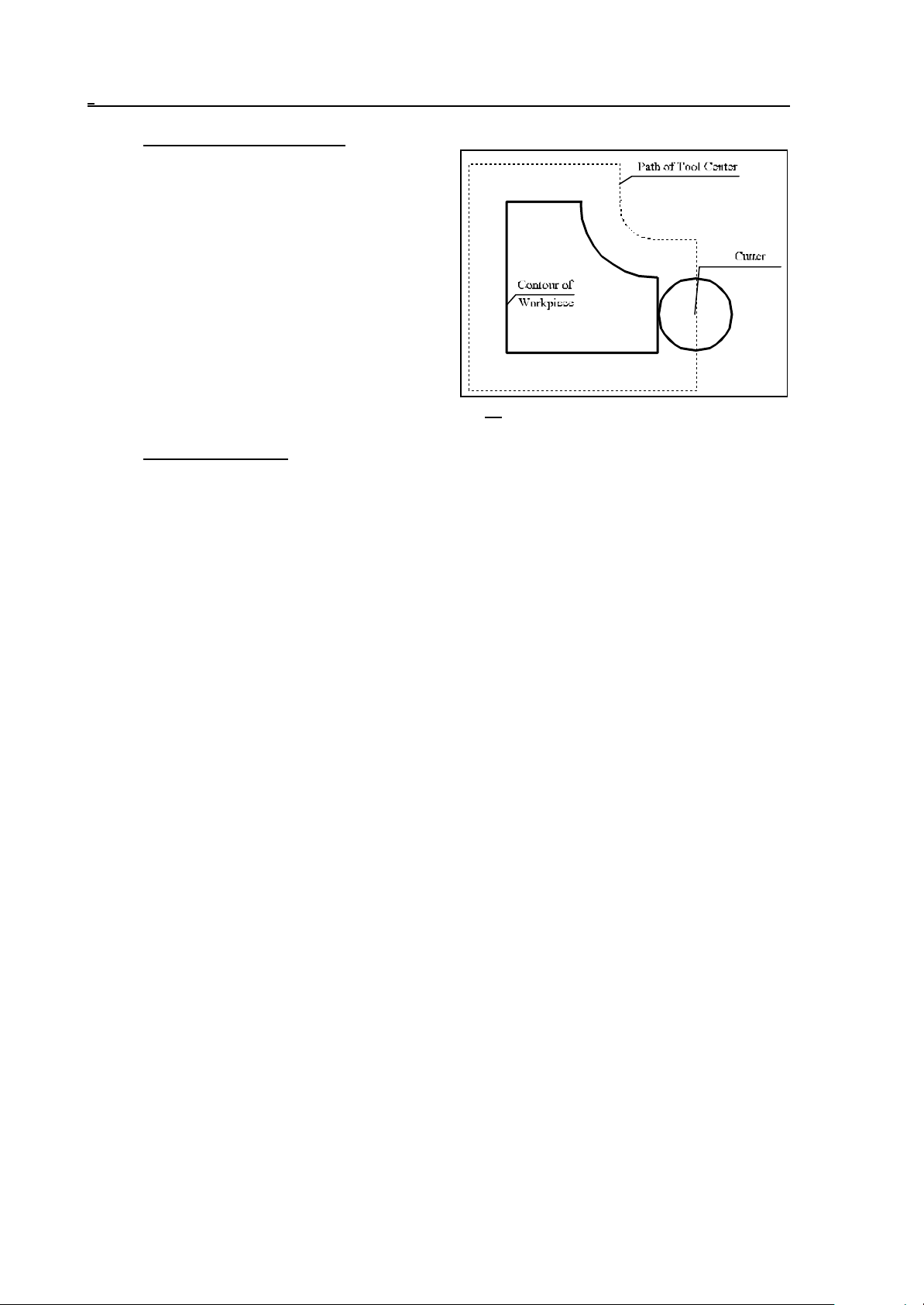
Cutter Radius Compensation
Machining a workpiece has to be done with tools
of different radii. Radius compensation has to be
introduced in order to write the actual contour data
of the part in the program, instead of the path
covered by the tool center (taking into
consideration the tool radii). The values of radius
compensations have to be set in control system.
Hereinafter reference can be made to cutter
compensations at address D in the program.
Fig. 1.2-9
Wear Compensation
The tools are exposed to wear in the course of machining. Allowance can be made for such
dimensional changes (in length and radius as well) with wear compensations. The tool wear can be
set in the control system. A geometry value, i.e., the initial length and radius of the tool, and a wear
one belong to each compensation group (referred to at address H or D). When the compensation is
set, the control will compensate the movement with the sum of the two values.
16
Page 17
2 Controlled Axes
2 Controlled Axes
Number of Axes (in basic configuration) 3 axes
In expanded configuration 5 additional axes (8 axes altogether)
Number of axes to be moved simultaneously 8 axes (with linear interpolation)
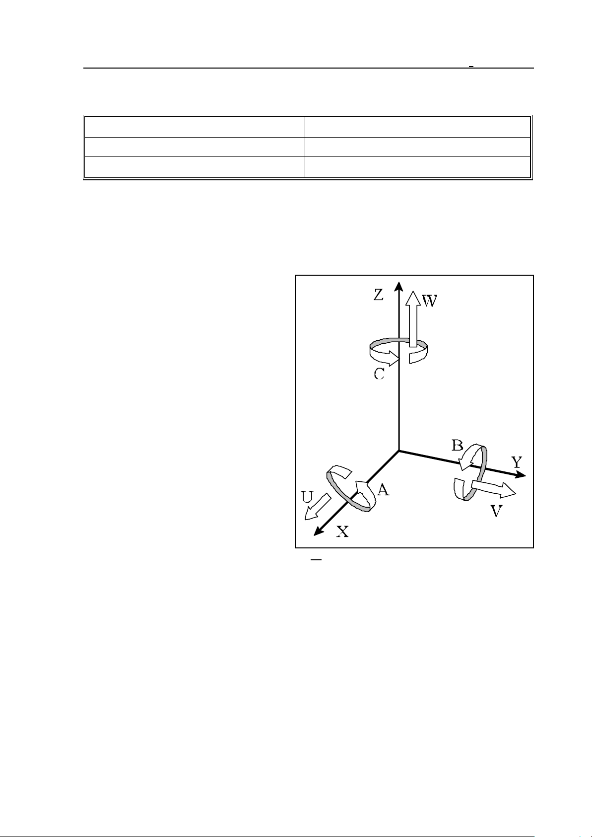
2.1 Names of axes
The names of controlled axes can be defined in the parameter memory. Each address can be
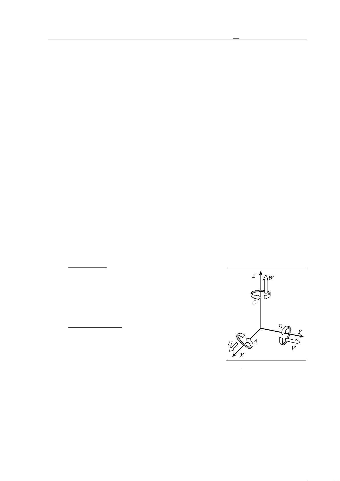
assigned to one of the physical axes.
In the basic configuration, the names of axes
in a milling control system: X, Y and Z.
The names of additional (expansion) axes
depend on their respective types.
Possible names of expansion axes
performing linear motions are: U,V and W.
When they are parallel to the main axes X,Y
and Z, their name will be U,V and W,
respectively.
Axes performing rotational motions are
termed A, B and C. The rotational axes
whose axle of rotation parallel to X, Y and
Z directions are termed A, B and C,
respectively.
Fig. 2.1-1
2.2 Unit and Increment System of Axes
The coordinate data can be specified in 8 digits. They can have signs, too. The positive sign + is
omitted.
The data of input length coordinates can be specified in mm or inches. They are the units of input
measures. The desired one can be selected from the program.
The path-measuring device provided on the machine can measure the position in mm or in inches. It
will determine the output unit of measures, which has to be specified by the control system as a
parameter. The two units of measures may not be combined on a given machine.
In the case of different input and output units of measures, the control system will automatically
perform the conversion.
17
Page 18
2 Controlled Axes
The rotational axes are always provided with degrees as units of measure.
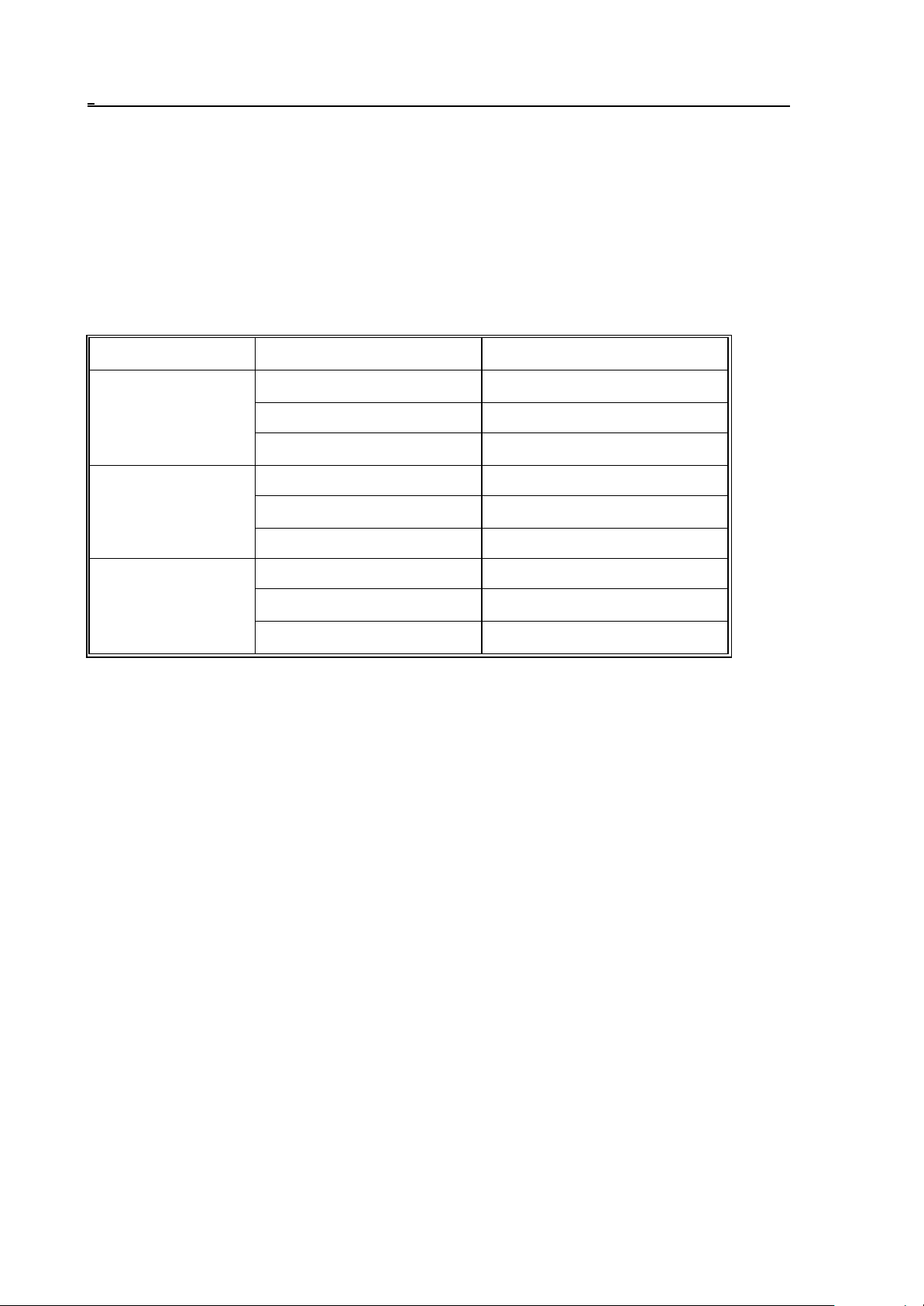
The input increment system of the control is regarded as the smallest unit to be entered. It can be
selected as parameter. There are three systems available - IS-A IS-B and IS-C. The increment
systems may not be combined for the axes on a given machine.
Having processed the input data, the control system will provide new path data for moving the axes.
Their resolution is always twice the particular input increment system. It is termed the output
increment system of the control.
Thus the input increment system of the control is determined by the resolution of the encoder.
Increment system Min. unit to be entered Max. unit to be entered
0.01 mm 999999.99 mm
IS-A
IS-B
IS-C
0.001 inch 99999.999 inch
0.01 degree 999999.99 degree
0.001 mm 99999.999 mm
0.0001 inch 9999.9999 inch
0.001 degree 99999.999 degree
0.0001 mm 9999.9999 mm
0.00001 inch 999.99999 inch
0.0001 degree 9999.9999 degree
18
Page 19
3 Preparatory Functions (G codes)
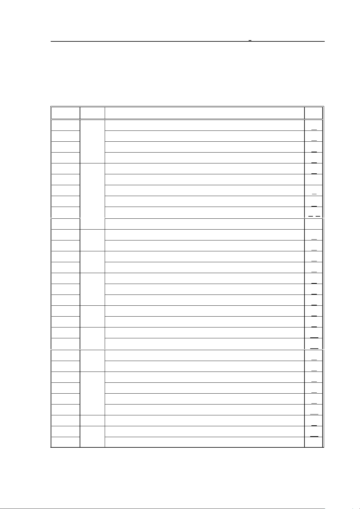
3 Preparatory Functions (G codes)
The type of command in the given block will be determined by address G and the number following
it.
The Table below contains the G codes interpreted by the control system, the groups and functions
thereof.
G code
G00
G01
Group
*
*
positioning 22
linear interpolation 22
Function
Page
01
G02 circular, helical interpolation, clockwise (CW) 24
G03 circular, helical interpolation, counter-clockwise (CCW) 24
G04
dwell 52
G05.1 multi-buffer mode on
G07.1 Cylindrical interpolation
35
00
G09 exact stop (in the given block) 49
G10 data setting (programmed)
59, 79
G11 programmed data setting cancel
G12.1
Polar coordinate interpolation on 31
26
G13.1 Polarc coordinate interpolation off 31
*
G15
polar coordinate command cancel 38
17
G16 polar coordinate command 38
*
G17
G18
*
selection of XpYp plane 62
02
selection of ZpXp plane 62
G19 selection of YpZp plane 62
G20
inch input 40
06
G21 metric input 40
*
G22
programable stroke check function on 158
04
G23 programable stroke check function off 158
*
G25
spindle speed fluctuation detection off 67
8
G26 spindle speed fluctuation detection on 67
G28
programmed reference-point return 53
G29 return from reference point 54
0
G30 return to the 1st, 2nd, 3rd and 4th reference point 54
G31 skip function 155
G33 01 thread cutting 29
G37
Automatic tool-length measurement 156
00
G38 cutter compensation vector hold 100
19
Page 20

3 Preparatory Functions (G codes)
G code
Group
Function
Page
G39 cutter compensation corner arc 100
*
G40
G41 cutter radius compensation left/3 dimensional tool compensation
cutter radius/3 dimensional tool compensation cancel
07
G42 cutter radius compensation right
*
G43
G44
G45
*
tool length compensation + 80
08
tool length compensation – 80
tool offset increase 81
85
85, 88
85, 88
G46 tool offset decrease 81
00
G47 tool offset double increase 81
G48 tool offset double decrease 81
*
G49
G50
*
08 tool length compensation cancel 80
scaling cancel 116
11
G51 scaling 116
*
G50.1
programable mirror image cancel 117
18
G51.1 programable mirror image 117
G52
local coordinate system setting 60
00
G53 positioning in the machine coordinate system 57
*
G54
work coordinate system 1 selection 58
G55 work coordinate system 2 selection 58
G56 work coordinate system 3 selection 58
14
G57 work coordinate system 4 selection 58
G58 work coordinate system 5 selection 58
G59 work coordinate system 6 selection 58
G61
exact stop mode 49
G62 automatic corner override mode 50
15
G63 override inhibit 50
*
G64
continuous cutting 50
G65 simple macro call 161
G66 macro modal call (A) in every motion command 162
G66.1 macro modal (B) call from each block 163
G67 macro modal call (A/B) cancel 162
G68
G69
*
coordinate system rotation 115
16
coordinate system rotation cancel 115
G73
G74 counter tapping cycle 139
High Speed Peck Drilling Cycle 138
09
G76 fine boring cycle 140
20
Page 21

3 Preparatory Functions (G codes)
G code
*
G80
G81 drilling, spot boring cycle, 141
G82 drilling, counter boring cycle 142
G83 peck drilling cycle 143
G84 tapping cycle 144
G84.2 rigid tap cycle 145
G84.3 rigid counter tap cycle 145
G85 boring cycle 148
G86 Boring Cycle Tool Retraction with Rapid Traverse 149
G87 Boring Cycle/Back Boring Cycle 150
G88 Boring Cycle (Manual Operation on the Bottom Point) 152
G89 Boring Cycle (Dwell on the Bottom Point, Retraction with Feed) 153
*
G90
*
G91
G92 00 work coordinates change/maximum spindle speed setting 59
*
G94
*
G95
Group
03
05
Function
canned cycle cancel 141
absolute command 38
incremental command 38
feed per minute 46
feed per revolution 46
Page
G96
*
G97
*
G98
G99 canned cycle R point level return 133
constant surface speed control 65
13
constant surface speed control cancel 65
canned cycle initial level return 133
10
L Notes:
– The * marked G codes in a group represent the state assumed by the control system after power-
on.
– If several codes are marked with * in a group, a parameter can be set to select the effective one
after power-on. They are : G00, G01; G17, G18; G43, G44, G49; G90, G91; G94, G95.
– At the time of power-on, the particular one of G20 and G21 will be effective, that has been set at
the time of power-off.
– Default interpretation of command G05.1 after power-on can be specified with the MULBUF
parameter.
– G codes in group 00 are not modal ones; the rest are so.
– More than one G code can be written in a block with the restriction that only one of the same
function group may used.
– Reference to an illegal G code or specification of several G codes belonging to the same group
within a particular block will produce error message 3005 ILLEGAL G CODE.
21
Page 22
4 The Interpolation
4 The Interpolation
4.1 Positioning (G00)
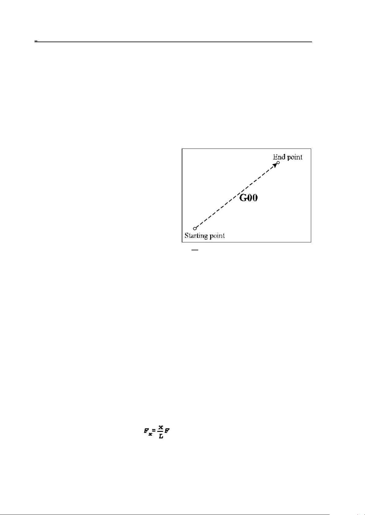
The series of instructions
G00 v
refers to a positioning in the current coordinate system.
It moves to the coordinate v. Designation v (vector) refers here (and hereinafter) to all controlled
axes used on the machine-tool. (They may be X, Y, Z, U, V, W, A, B, C)
The positioning is accomplished along a straight line involving the simultaneous movements of all axes
specified in the block. The coordinates may be absolute or incremental data.
The speed of positioning cannot be commanded in
the program because it is accomplished with
different values for each axis, set by the builder of
machine-tool as a parameter. When several axes
are being moved at a time, the vectorial resultant of
speed is computed by the control system in such a
way that positioning is completed in a minimum
interval of time, and the speed will not exceed
anywhere the rapid traverse parameter set for each
axis.
In executing the G00 instruction, the control system
performs acceleration and declaration in starting
and ending the movements, respectively. On completion of the movement, the control will check the
"in position" signal when parameter POSCHECK in the field of parameters is 1, or will not do so
when the parameter is set to 0. It will wait for the "in position" signal for 5 seconds, unless the signal
arrives, the control will return the 1020 POSITION ERROR message. The maximum acceptable
deviation from the position can be specified in parameter INPOS.
Being a modal code, G00 remains effective until it is re-written by another interpolation command.
After power-on, G00 or G01 is effective, depending on the value set in parameter group CODES of
the parameter field.
Fig. 4.1-1
4.2 Linear Interpolation (G01)
The series of instructions
G01 v F
will select a linear interpolation mode. The data written for v may be absolute or incremental values,
interpreted in the current coordinate system. The speed of motion (the feed) can be programmed at
address F.
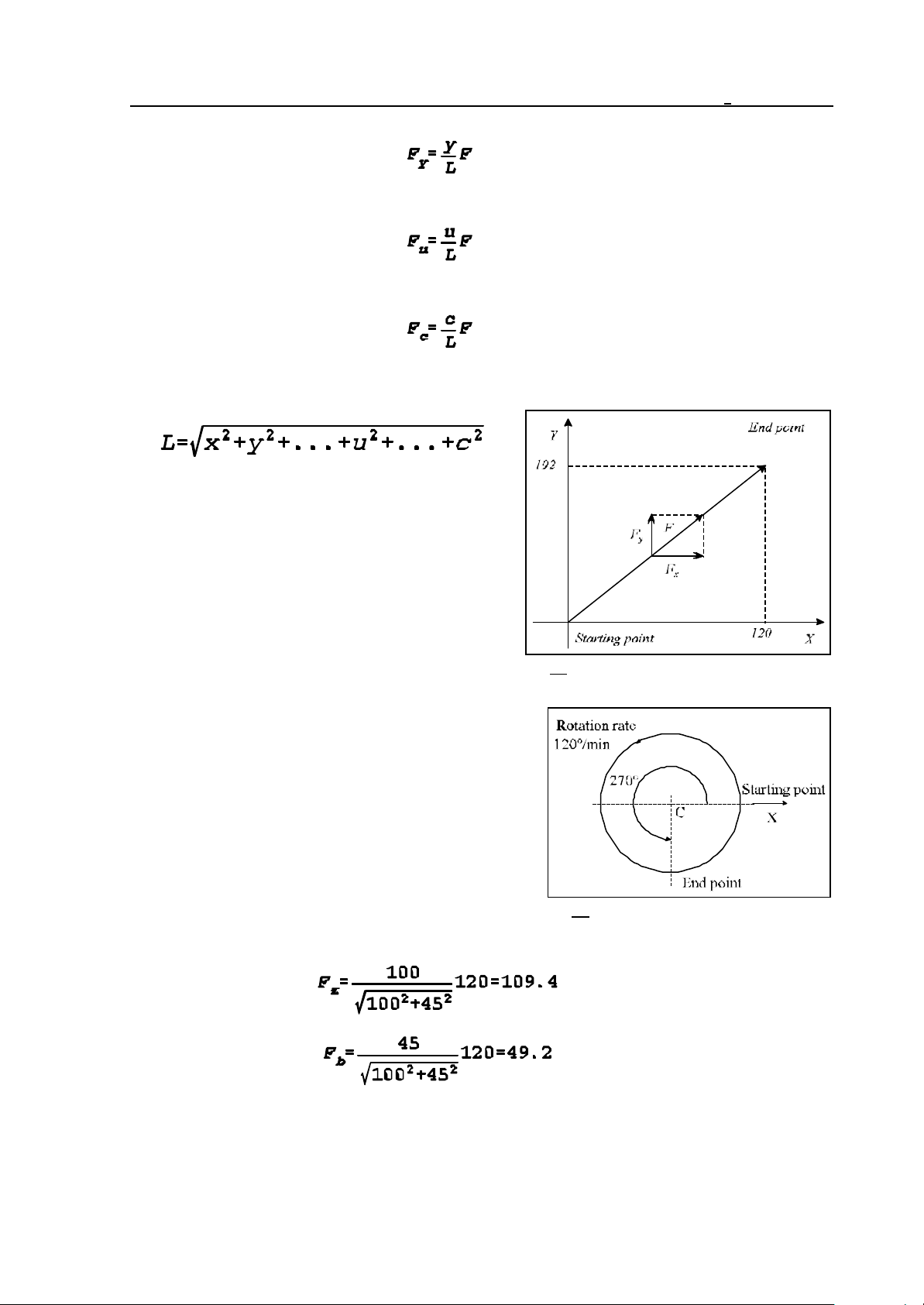
The feed programmed at address F will be accomplished invariably along the programmed path. Its
axial components:
Feed along the axis X is
22
Page 23
4 The Interpolation
Feed along the axis Y is
.............................
Feed along the axis U is
.............................
Feed along the axis C is
where x, y, u, c are the displacements programmed along the respective axes, L is the vectorial
length of programmed displacement:
G01 X100 Y80 F150
Fig. 4.2-1
The feed along a rotational axis is interpreted in units of
degrees per minute (°/min):
G01 B270 F120
In the above block, F120 means 120deg/minute.
If the motion of a linear and a rotary axis is combined
through linear interpolation, the feed components will be
distributed according to the above formula. E.g. in block
G91 G01 Z100 B45 F120
Fig. 4.2-2
feed components in Z and B directions are:
feed along axis Z: mm/min
feed along axis B:
°/min
Being a modal code, G01 is effective until rewritten by another interpolation command. After
power-on, G00 or G01 is effective, depending on the parameter value set in group CODES of the
parameter field.
23
Page 24
4 The Interpolation
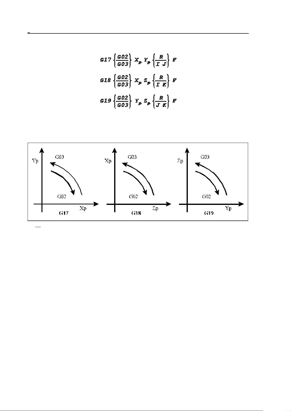
4.3 Circular and Spiral Interpolation (G02, G03)
The series of instructions specify circular interpolation.
A circular interpolation is accomplished in the plane selected by commands G17, G18, G19 in
clockwise or counter-clockwise direction (with G02 or G03, respectively).
Fig. 4.3-1
Here and hereinafter, the meanings of Xp, Yp, and Zp are:
Xp: axis X or its parallel axis,
Yp: axis Y or its parallel axis,
Zp: axis Z or its parallel axis.
The values of Xp, Yp, and Zp are the end-point coordinates of the circle in the given coordinate
system, specified as absolute or incremental data.
24
Page 25
4 The Interpolation
Further data of the circle may be specified in one of two different ways.
Case 1
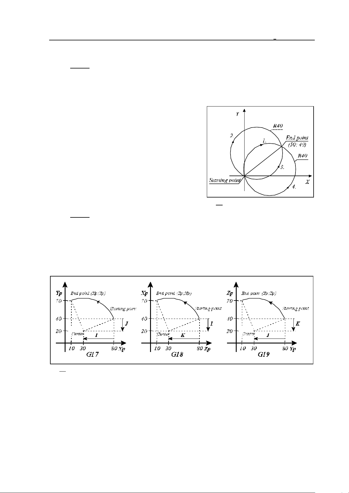
At address R where R is the radius of the circle. Now the control will automatically calculate the
coordinates of the circle center from the start point coordinates (the point where the control is in the
instant of the circle block being entered), the end point coordinates (values defined at addresses Xp,
Yp, Zp) and from the programmed circle radius R. Since
two different circles of radius R can be drawn between
the start and the end points for a given direction of
circumventing (G02 or G03), the control will interpolate
an arc smaller or larger than 180° when the radius of the
circle is specified as a positive or a negative number,
respectively. For example:
Arc section 1: G02 X50 Y40 R40
Arc section 2: G02 X50 Y40 R-40
Arc section 3: G03 X50 Y40 R40
Arc section 4: G03 X50 Y40 R-40
Fig. 4.3-2
Case 2
The circle center is specified at address I, J, K for the Xp, Yp and Zp axes. The values specified at
addresses I, J, K are interpreted always incrementally by the control system, so that the vector
defined by the values of I, J, K points from the start point to the center of the circle. For example:
With G17: G03 X10 Y70 I-50 J-20
With G18: G03 X70 Z10 I-20 K-50
With G19: G03 Y10 Z70 J-50 K-20
Fig. 4.3-3
25
Page 26
4 The Interpolation
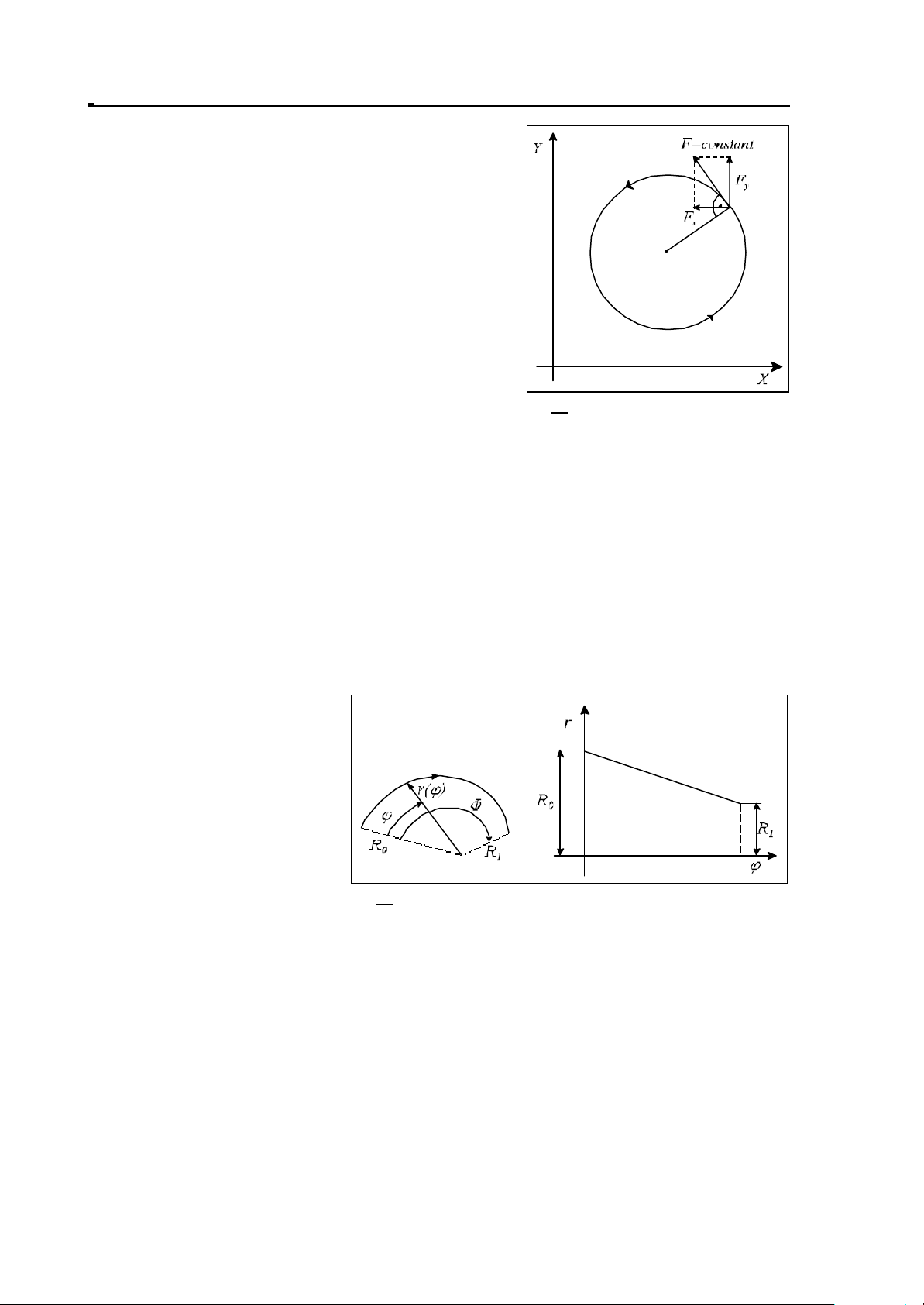
The feed along the path can be programmed at address F,
pointing in the direction of the circle tangent, and being
constant all along the path.
L Notes:
– I0, J0, K0 may be omitted, e.g.
G03 X0 Y100 I-100
– When each of Xp, Yp and Zp is omitted, or the end point
coordinate coincides with the start point coordinate,
then:
a. If the coordinates of the circle center are
programmed at addresses, I, J, K the
control will interpolate a complete circle of
Fig. 4.3-4
360°. E.g.: G03 I-100,
b. If radius R is programmed, the control returns error 3012 ERRONEOUS CIRCLE DEF.
R.
– When the circle block
a. does not contain radius (R) or I, J, K either,
b. or reference is made to address I, J, K outside the selected plane, the control returns
3014 ERRONEOUS CIRCLE DEF. error. E.g. G03 X0 Y100, or (G18) G02 X0
Z100 J-100.
– The control returns error message 3011 RADIUS DIFFERENCE whenever the difference
between the start-point and end-point radii of the circle defined in block G02, G03 exceeds
the value defined in parameter RADDIF.
Whenever the difference of radii is
smaller than the value specified in
the above parameter, the control
will move the tool along a spiral
path in which the radius is varying
linearly with the central angle.
The angular velocity, not the one
tangential to the path will be
constant in the interpolation of a
circle arc of a varying radius.
Fig. 4.3-5
26
Page 27
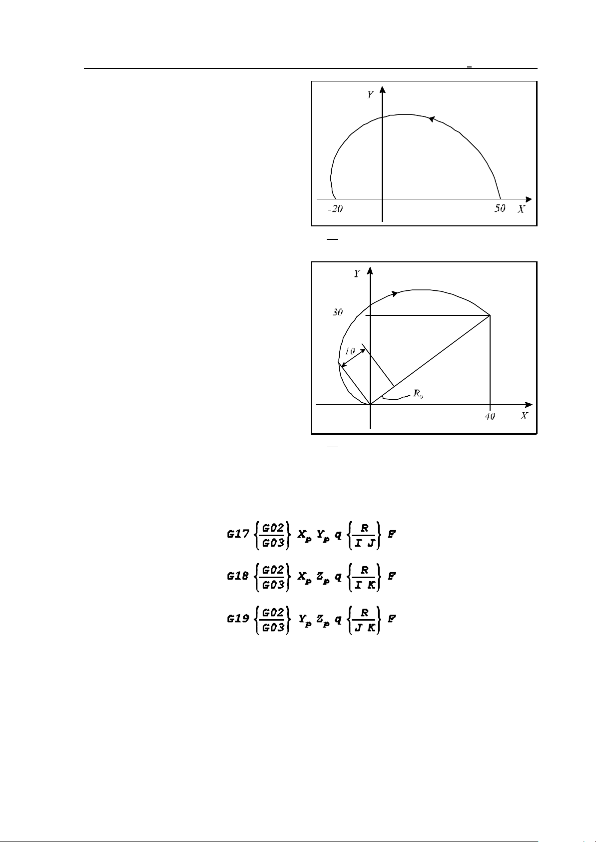
The program detail below is an example of how
a spiral interpolation (circle of varying radius)
can be specified by the use of addresses I, J, K.
G17 G90 G0 X50 Y0
G3 X-20 I-50
If the specified circle radius is smaller than half
the distance of straight line inter-connecting the
start point with the end point, the control will
regard the specified radius of the circle as the
start-point radius, and will interpolate a circle of
a varying radius (spiral), whose center point is
located on the straight line connecting the start
point with the end point, at distance R from the
start point.
G17 G0 G90 X0 Y0
G2 X40 Y30 R10
4 The Interpolation
Fig. 4.3-6
Fig. 4.3-7
4.4 Helical Interpolation (G02, G03)
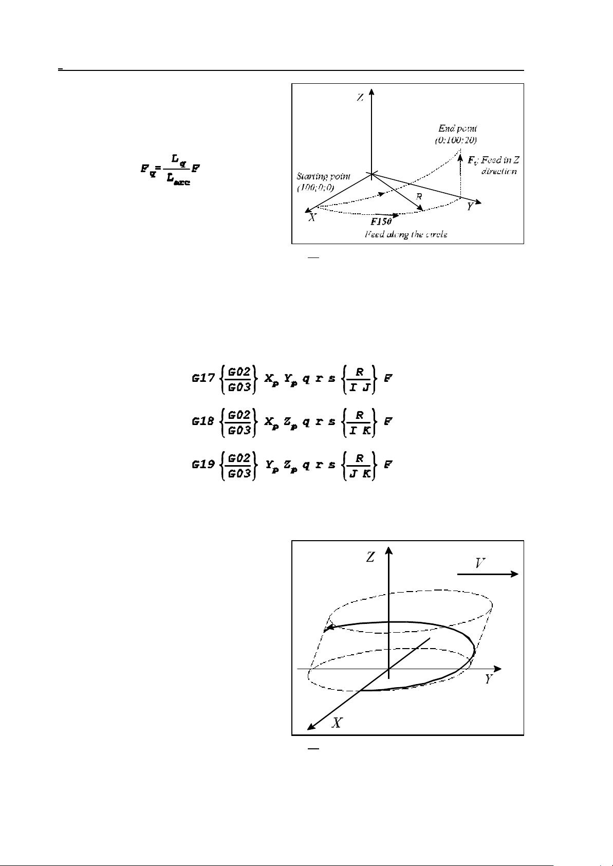
The series of instructions will define a helical interpolation.
It is distinguished from circular interpolation that a third axis (q), which is not an axis composing the
circular plane. The control performs a simple movement along axis q.
27
Page 28
4 The Interpolation
The feed specified at address F is effective
along the circle path. Feed component Fq along
axis q is obtained from the relationship
where
Lq: displacement along axis q,
L
: length of circular arc,
arc
F: programmed feed,
Fq: feed along axis q.
For example:
G17 G03 X0 Y100 Z20 R100 F150
The series of instructions
Fig. 4.4-1
define a multi-dimensional spatial helical interpolation in which q, r, s are optional axes not involved
in the circle interpolation.
For example, series of instructions
G17 G3 X0 Y-100 Z50 V20 I-100
will move the tool along the superficies of an
oblique cylinder if V is an axis parallel to Y.
L Notes:
– Whenever parameter HELICALF in the field
of parameters is set to 1, the control will
implement the programmed feed along
the spatial path.
– In the case of the circle specified in the
selected plane having a varying radius,
the interpolation will be carried out
along the superficies of the specified
Fig. 4.4-2
cone.
28
Page 29
4 The Interpolation
– The specified tool-radius compensation is implemented invariably in the plane of the circle.
4.5 Equal Lead Thread Cutting (G33)
The instruction
G33 v F Q
G33 v E Q
will define a straight or taper thread cutting of equal lead.
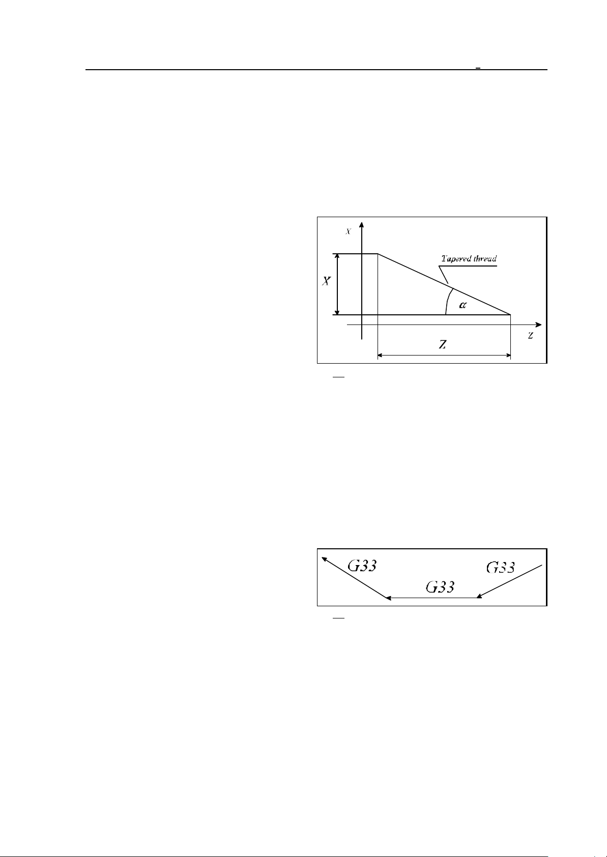
The coordinates of maximum two axes can be
written for vector v. The control will cut a
tapered thread if two coordinated data are
assigned to vector v. The control will take the
lead into consideration along the long axis.
If "<45°, i.e. Z>X, the programmed lead will
be taken into account along axis Z,
if ">45°, i.e. X>Z, the control will take the
programmed lead along axis X.
The lead can be defined in one of two 2 ways.
– If the lead is specified at address F, the data
will be interpreted in mm/rev or
Fig. 4.5-1
inch/rev. Accordingly, F2.5 has to be
programmed if a thread of 2.5 mm lead is to be cut.
– If the pitch is specified at address E, the control will cut an inch thread. Address E is interpreted
as number of ridges per inch. If, e.g., E3 is programmed, the control will cut a thread
a"=25.4/3=8.4667mm lead.
The shift angle of the thread start is specified at address Q expressed in degrees from the zero pulse
of the spindle encoder. A multiple thread can be cut by an adequate programming of the value of Q,
i.e., the control can be programmed here for the particular angular displacements of the spindle, at
which the various threads are to be cut. If, e.g., a double thread is to be cut, the first and the second
starts will be commenced from Q0 (no special programming is needed) and from Q180,
respectively.
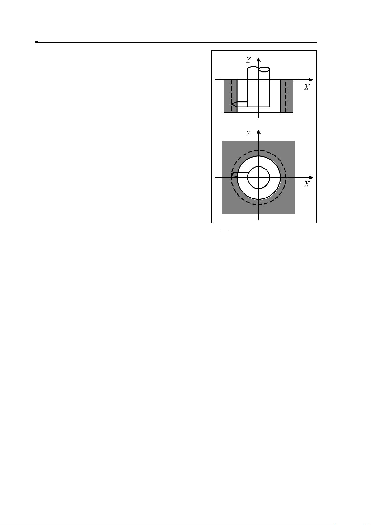
G33 is a modal function. If several threadcutting blocks are programmed in succession,
threads can be cut in any arbitrary surface
limited by straight lines.
Fig. 4.5-2
The control is synchronized to the zero pulse of the spindle encoder in the first block, no
synchronization will be performed in the subsequent blocks resulting in a continuous thread in each
section of lines. Hence the programmed shift angle of the thread start (Q) will also be taken into
account in the first block.
29
Page 30
4 The Interpolation
An example of programming a thread-cutting:
N50 G90 G0 X0 Y0 S100 M4
N55 Z2
N60 G33 Z-100 F2
N65 M19
N70 G0 X5
N75 Z2 M0
N80 X0 M4
N85 G4 P2
N90 G33 Z-100 F2
...
Explanation:
N50, N55 - Moving the tool over the center of hole, starting
the spindle in counter-clockwise rotation,
N60 - First thread-cutting cycle, (lead 2mm),
N65 - Oriented spindle stop (the spindle is stopped in a
fixed position),
N70 - Tool retraction along axis X,
N75 - Tool retraction to the top of hole, programmed stop,
the operator adjust the tool to the next thread-cutting
cycle,
N80 - Return to the center of hole, re-start of spindle,
N85 - Waiting for the speed to be assumed by the spindle,
N90 - Second thread-cutting cycle.
Fig. 4.5-3
L Notes:
– The control returns error message 3020 DATA DEFINITION ERROR G33 if more than two
coordinates are specified at a time in the thread-cutting block, or if both addresses F and E
are specified simultaneously.
– Error message 3022 DIVIDE BY 0 IN G33 is produced when 0 is specified for address E in the
thread-cutting block.
– An encoder has to be mounted on the spindle for the execution of command G33.
– In the course of command G33 being executed, the control will take the feed and spindle override
values automatically to be 100%; the effect of the stop key will only prevail after the block
has been executed.
– On account of the following error of the servo system, overrun and run out allowances have to be
provided for the tool in addition to the part at the beginning and end of the thread in order to
obtain a constant lead all along the part.
– In the course of thread-cutting the feed (in mm/minute) may not exceed the value selected in the
group of parameters FEEDMAX.
– In the course of thread-cutting the speed (r.p.m) of the spindle may not exceed the maximum
speed permissible for the spindle encoder mechanically and electrically (the maximum output
frequency).
30
Page 31
4.6 Polar Coordinate Interpolation (G12.1, G13.1)
4.6 Polar Coordinate Interpolation (G12.1, G13.1)
Polar coordinate interpolation is a control operation method, in case of which the work described in
a Cartesian coordinate system moves its contour path by moving a linear and a rotary axis.
Command
G12.1
switches polar coordinate interpolation mode on. The path of the milling tool can be described in the
succeeding part program in a Cartesian coordinate system in the usual way by programming linear
and circular interpolation, by taking the tool radius compensation into account. The command must
be issued in a separate block and no other command can be written beside.
Command
G13.1
switches polar coordinate interpolation mode off. The command must be issued in a separate
block and no other command can be written beside. It always registers state G13.1 after power-
on or reset.
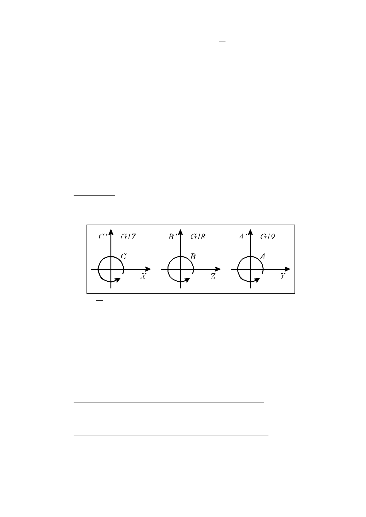
Plane selection
A plane determining the address of the linear and the rotary axis to be applied must be selected
before switching polar coordinate interpolation on.
Fig. 4.6-1
Command
G17 X_ C_
selects axis X for linear axis, while as for the rotary axis it is axis C. The virtual axis is indicated with
C’ on the diagram, the programming of which is implemented by defining length measures.
With the help of commands
G18 Z_ B_
G19 Y_ A_
further linear and rotary axes can be selected together in the above mentioned way.
Work zero point offset in the course of polar coordinate interpolation
In case of using polar coordinate interpolation the origin of the applied work coordinate system must
be chosen so that it coincides with the rotation axis of the circular axis.
Position of the axes when polar coordinate interpolation is switched on
Before switching polar coordinate interpolation on (command G12.1) make sure that the circular
axis position is 0. The linear axis position can either be negative or positive but it cannot be 0.
31
Page 32

4.6 Polar Coordinate Interpolation (G12.1, G13.1)
Programming length coordinates in the course of polar coordinate interpolation
In the switched-on state of the polar coordinate interpolation length coordinate data may be
programmed on both axes belonging to the selected plane; The rotary axis in the selected plane
functions as the second (virtual) axis. If e.g. axes X and C have been selected by means of
command G17 X_ C_ address C can be programmed like axis Y in the case of plane selection G17
X_ Y_.
The programming of the first axis being in diameter does not influence the programming of the
virtual axis, the coordinate data must always be given in radius for the virtual axis. If, e.g., polar
coordinate interpolation is executed in plane X C the value written at address C must be specified in
radius, independent of address X given in diameter or radius.
Move of axes not taking part in polat coordinate interpolation
The tool on these axes moves normally, independent of the switched-on state of the polar
coordinate interpolation.
Programming circular interpolation in the course of polar coordinate interpolation
Definition of a circle in polar coordinate interpolation mode is possible as known by means of the
radius or by programming the circle center coordinates. In the latter case addresses I, J, K must be
used according to the selected plane as seen below:
G17 X_ C_
G12.1
...
G2 (G3) X_ C_ I_ J_
G18 Z_ B_
G12.1
...
G2 (G3) B_ Z_ I_ K_
G19 Y_ A_
G12.1
...
G2 (G3) Y_ A_ J_ K_
Use of tool radius compensation in case of polar coordinate interpolation
Commands G41, G42 can be used customary in polar coordinate interpolation. The following
restrictions must be considered regarding its application:
– Switch-on of polar coordinate interpolation (command G12.1) is only possible in state G40,
– If G41 or G42 is switched on in state G12.1, G40 must be programmed before switching polar
coordinate interpolation off (command G13.1).
Programming restrictions in the course of polar coordinate interpolation
The below commands cannot be used in the switched-on state of polar coordinate interpolation:
– plane change: G17, G18, G19,
– coordinate transformations: G52, G92,
– work coordinate system change: G54, ..., G59,
– orientation in machine coordinate system: G53.
Feed in the course of polar coordinate interpolation
Interpretation of feed in polar coordinate interpolation is tangential speed as in case of right angle
interpolation: The relative speed of piece and tool is defined.
With polar coordinate interpolation the path described in a Cartesian coordinate system is done by
moving a linear and a rotary axis. As the tool center approaches the circular axis of rotation, the
rotary axis should have to take larger and larger steps within a time unit so that the path speed is
constant. However the maximum speed permitted for the rotary axis defined by parameter limits
circular axis speed. Therefore, near to the origin the control decreases feed step by step for the
rotary axis speed not to exceed all limits.
32
Page 33
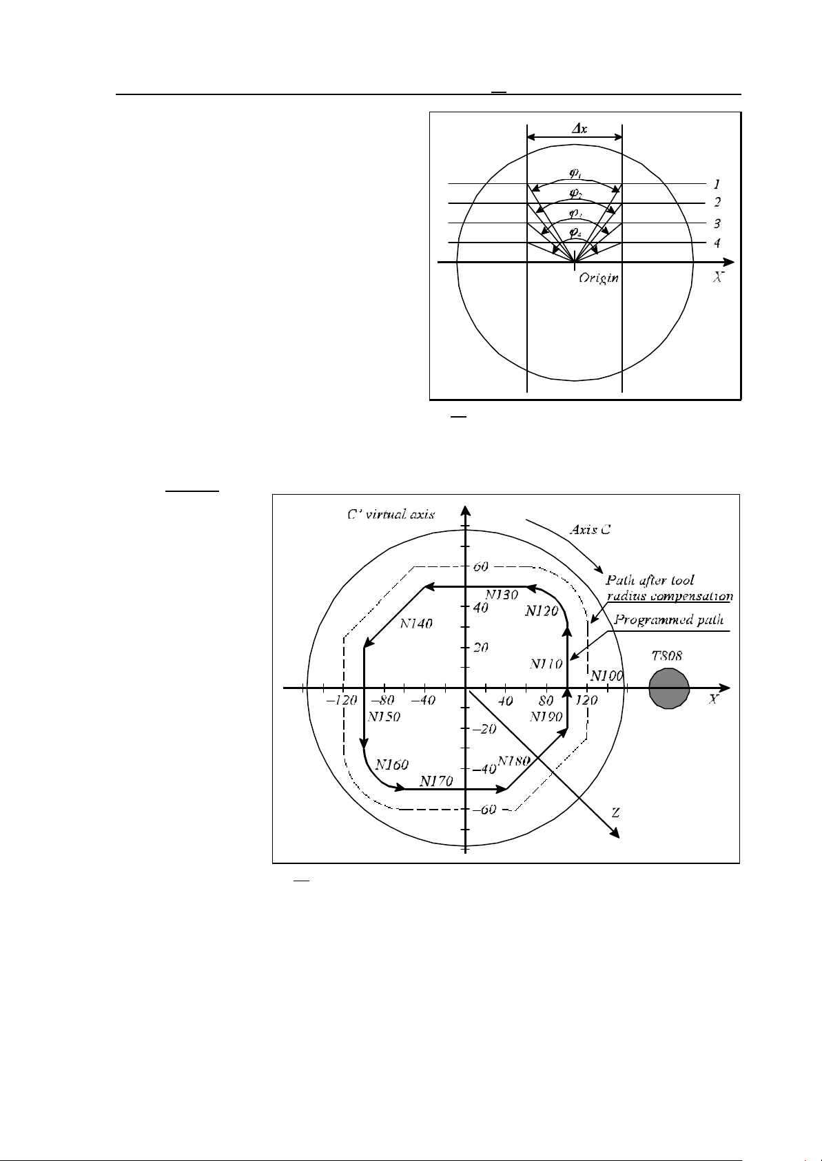
The diagram beside shows the cases when
straight lines parallel to axis X (1, 2, 3, 4) are
programmed. )x move belongs to the
programmed feed within a time unit. Different
angular moves (n1, n2, n3, n4) belong to )x
move for each straight lines (1, 2, 3, 4).
Apparently, the closer the machining gets to the
origin the larger angular movement the rotary
axis has to make within a time unit in order to
keep the programmed feed.
In case the angular move to be made within a
time unit exceeds the value of parameter
FEEDMAX set for rotary axis the control
gradually decreases the tangential feed.
With these in mind, programs in case of which
the tool center moves close to the origin are to
be avoided.
Example
Below an example for
the use of polar
coordinate
interpolation is shown.
The axes taking part
in the interpolation:
Axes X (linear axis)
and C (rotary axis).
Axis X is
programmed in
diameter, while that of
axis C is in radius.
4.6 Polar Coordinate Interpolation (G12.1, G13.1)
Fig. 4.6-2
Fig. 4.6-3
%O7500(POLAR COORDINATE INTERPOLATION)
...
N050 T808
N060 G59 (start position of coordinate system G59 in
33
Page 34

4.6 Polar Coordinate Interpolation (G12.1, G13.1)
direction X on rotary axis C)
N070 G17 G0 X200 C0 (select plane X, C; orientation to coordinate
X…0, C=0)
N080 G94 Z-3 S1000 M3
N090 G12.1 (polar coordinate interpolation on)
N100 G42 G1 X100 F1000
N110 C30
N120 G3 X60 C50 I-20 J0
N130 G1 X-40
N140 X-100 C20
N150 C-30
N160 G3 X-60 C-50 R20
N170 G1 X40
N180 X100 C-20
N190 C0
N200 G40 G0 X150
N210 G13.1 (polar coordinate interpolation off)
N220 G0 G18 Z100 (Retract tool, select plane X, Z)
...
%
34
Page 35
4.7 Cylindrical Interpolation (G7.1)
4.7 Cylindrical Interpolation (G7.1)
Should a cylindrical cam grooving be milled on a cylinder mantle, cylindrical interpolation is to be
used. In this case the rotation axis of the cylinder and of a rotary axis must coincide. The rotary axis
movements are specified in the program in degrees, which are converted into linear movement along
the mantle by the control in function of the cylinder radius, so that linear and circular interpolation
can be programmed together with another linear axis. The movements resulted after the
interpolations, are re-converted into movement in degrees for the rotary axis.
Command cylindrical interpolation on
G7.1 Qr
switches cylindrical interpolation on, where
Q: address of rotary axis taking part in the cylindrical interpolation,
r: cylinder radius.
If for example the rotary axis acting in cylindrical interpolation is axis C and the cylinder radius is 50
mm, cylindrical interpolation is switched on by means of command G7.1 C50.
In the succeeding part program the path to be milled on the cylinder mantle can be described by
specifying linear and circular interpolation. The coordinate for the linear axis must be given in mm,
while that of the rotary axis in degrees (°).
Command cylindrical interpolation off
G7.1 Q0
switches cylindrical interpolation off, i.e. code G corresponds to that of the switch-on, except for the
address of rotary axis being 0.
The cylindrical interpolation indicated in the above example (G7.1 C50) can be switched off with the
help of command G7.1 C0.
Command G7.1 must be issued in a separate block.
Plane selection
The plane selection code is always determined by the name of the
linear axis parallel to the rotary axis. The rotary axes parallel to
axes X, Y and Z are axes A, B and C, respectively.
G17 X A or
G17 B Y
G18 Z C or
G18 A X
G19 Y B or
G19 C Z
Circular interpolation
It is possible to define circular interpolation in cylindrical
interpolation mode, however only by specifying radius R.
No circular interpolation can be executed in case of
cylindrical interpolation by giving the circle center (I, J, K).
The circle radius is always interpreted in mm or inch, never in
Fig. 4.7-1
degree.
For example circular interpolation between axes Z and C can be specified in two ways:
G18 Z_ C_
G2 (G3) Z_ C_ R_
G19 C_ Z_
G2 (G3) C_ Z_ R_
35
Page 36
4.7 Cylindrical Interpolation (G7.1)
Application of tool radius compensation in case of cylindrical interpolation
Commands G41, G42 can be used in the usual manner in the switched-on state of cylindrical
interpolation. Though the following restrictions are in effect regarding its application:
– Switch-on of cylindrical interpolation (command G7.1 Qr) is only possible in state G40.
– Should G41 or G42 be switched on in cylindrical interpolation mode, G40 must be programmed
before switching cylindrical interpolation off (command G7.1 Q0).
Programming restrictions in the course of cylindrical interpolation
The following commands are not available in the switched-on state of cylindrical interpolation:
– plane selection: G17, G18, G19,
– coordinate transformations: G52, G92,
– work coordinate system change: G54, ..., G59,
– positioning in machine coordinate system: G53,
– circular interpolation by giving circle center (I, J, K),
– drilling cycles.
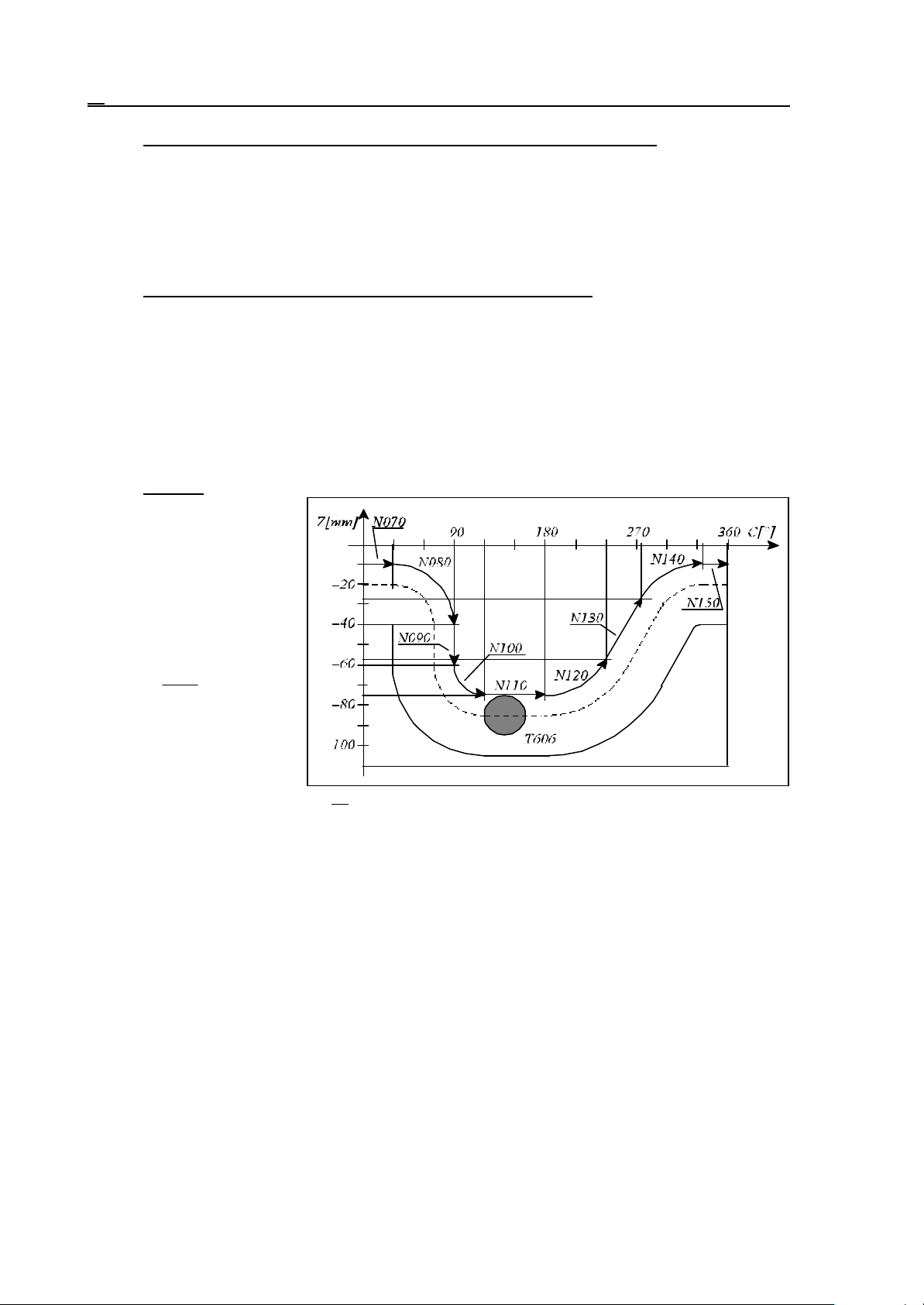
Example
The diagram beside shows a
path milled 3 mm deep on
the mantle of an R=28.65mm-radial cylinder. Rotating
tool T606 is parallel to the
axis X.. 1° movement on the
cylinder mantle is:
1
2865
mm mm
⋅
180
°
°
⋅ =
π
05. .
The axis order seen on the
diagram corresponds to
plane selection G19.
%O7602(CYLINDRICAL INTERPOLATION)
...
N020 G0 X200 Z20 S500 M3 T606
N030 G19 Z-20 C0 (G19: select plane C–Z)
N040 G1 X51.3 F100
N050 G7.1 C28.65 (cylindrical interpolation on, rotary
N060 G1 G42 Z-10 F250
N070 C30
N080 G2 Z-40 C90 R30
N090 G1 Z-60
N100 G3 Z-75 C120 R15
N110 G1 C180
N120 G3 Z-57.5 C240 R35
N130 G1 Z-27.5 C275
Fig. 4.7-2
axis: C, cylinder radius: 28.65mm)
36
Page 37

4.7 Cylindrical Interpolation (G7.1)
N140 G2 Z-10 C335 R35
N150 G1 C360
N160 G40 Z-20
N170 G7.1 C0 (cylindrical interpolation off)
N180 G0 X100
...
%
37
Page 38
5 The Coordinate Data
5 The Coordinate Data
5.1 Absolute and Incremental Programming (G90, G91), Operator I
The input coordinate data can be specified as absolute or incremental values. In an absolute
specification, the coordinates of the end point have to be specified for the control, for an incremental
data, it is the distance to go in the block.
G90: Programming of absolute data
G91: Programming of incremental data
G90 and G91 are modal functions. Parameter CODES will decide which state will be assumed by
the control system at the time of power-on.
Movement to an absolute position is only feasible after a reference point return.
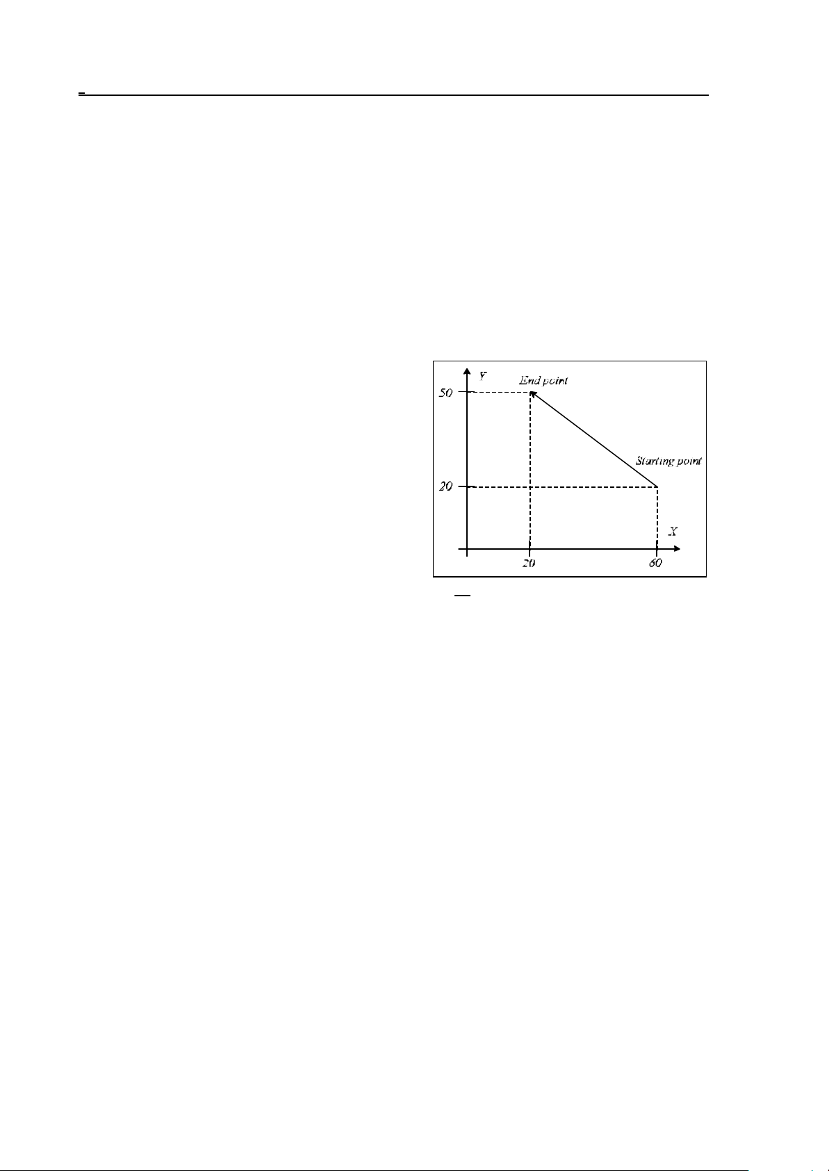
Example:
As shown in the Figure, a movement can be
programmed in one of two different ways.
G90 G01 X20 Y50
G91 G01 X-40 Y30
Operator I will be effective under the conditions of an
absolute data specification. It is only applicable to the
coordinate, whose address precedes it. It means an
incremental data. The alternative way of solving the
above example:
(G90) G01 XI-40 YI30
G01 X20 YI30
G01 XI-40 Y50
Fig. 5.1-1
5.2 Polar Coordinates Data Command (G15, G16)
Alternatively, the coordinates of the end point can be entered with polar coordinate data
specification, i.e., with the specification of angle and radius.
G16: Polar coordinate data command
G15: Polar coordinate data command cancel
The control is in G15 state after power on. G15 and G16 are modal functions.
The data of polar coordinates are effective in the plane defined by G17, G18, G19. When a data is
specified, the addresses of the plane's horizontal and vertical axes are regarded as radius and angle,
respectively. For example, in G17 sate, the data written at addresses X(U) and Y(V) are the radius
and angle, respectively. CAUTION! In state G18, Z and X are the horizontal and the vertical axes
(data of R and angle, respectively).
When an angular data is specified, the positive and the negative directions of the angle are counterclockwise and clockwise, respectively.
The data of the rest of axes will be assumed to be Cartesian coordinate data. The radius and the
angle can be specified both as absolute and as incremental data.
When the radius is specified as an absolute data, the origin of the current coordinate system will be
the origin of the polar coordinate system:
38
Page 39
5 The Coordinate Data
Example:
G90 G16 G01 X100 Y60 F180
Both the radius and the angle are
absolute data, the tool moves to the
point of 100mm; 60°.
G90 G16 G01 X100 YI40 F180
The angle is an incremental data. A
movement by 40° relative to the
previous angular position is moved.
With the radius, specified as an
Fig. 5.2-1
incremental value, the instantaneous
position of the axes will be the origin
of the polar coordinate system.
A circle can be programmed with
polar coordinate data command
(G16). The circle can be also specified
with the radius and I, J, K as well. In
the latter case, however, the control
will regard addresses I, J, K invariably
as Cartesian data. When the origin of
the current coordinate system
coincides with the center of a circle or
Fig. 5.2-2
a helix, a multiple turn one can also be
programmed with polar coordinate data specification.
Example:
(G17 G16 G90) G02 X100 Y-990 Z50 R-100
A helix of 2¾ turns has been specified in the above block in counter-clockwise direction of rotation.
In programming a multiple-turn circle, bear in mind that a negative or a positive polar angle has to be
programmed for direction G2 or G3, respectively.
L Notes:
The addresses encountered in the following instructions will not be regarded as polar coordinate
specifications even when state G16 is:
– G10 coordinates encountered in setting instruction,
– G52 coordinate offset,
– G92 coordinate setting,
– G53 positioning in machine coordinate system,
– G68 coordinate rotation,
– G51 scaling on,
– G50.1 programmable mirror image.
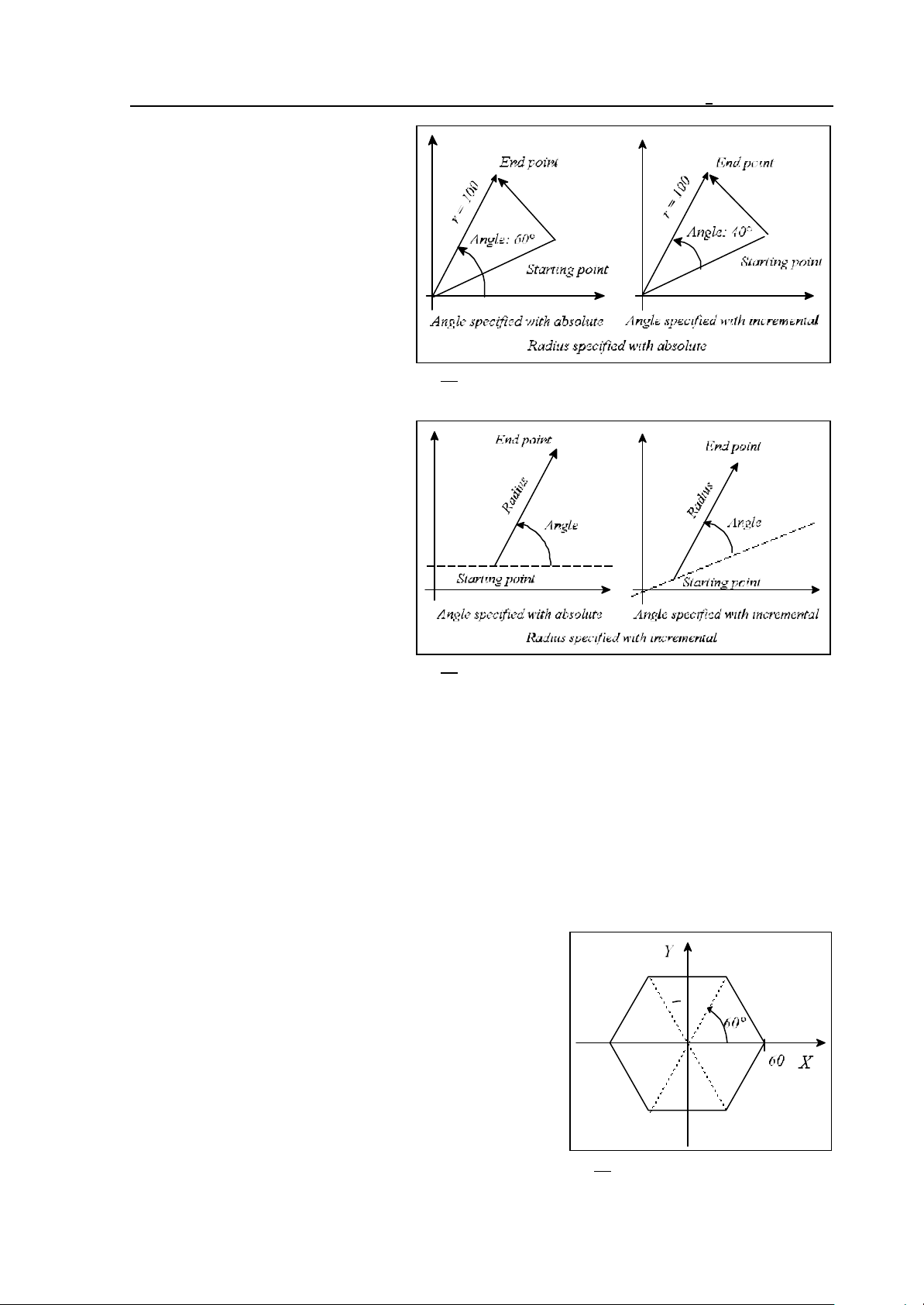
An example of milling a hexagon:
N1 G90 G17 G0 X60 Y0 F120
N2 G16 G1 Y60
Fig. 5.2-3
39
Page 40

5 The Coordinate Data
N3 Y120
N4 Y180
N5 Y240
N6 Y300
N7 Y360
N8 G15 G0 X100
5.3 Inch/Metric Conversion (G20, G21)
With the appropriate G code programmed, the input data can be specified in metric or inch units.
G20: Inch input programming
G21: Metric input programming
At the beginning of the program, the desired input unit has to be selected by specifying the
appropriate code. The selected unit will be effective until a command of opposite meaning is issued,
i.e., G20 and G21 are modal codes. Their effect will be preserved even after power-off, i.e., the unit
prevailing at the time of power-off will be effective after power-on.
The change of the unit will affect the following items:
– Coordinate and compensation data,
– Feed,
– Constant surface speed
– Position, compensation and feed displays.
5.4 Specification and Value Range of Coordinate Data
Coordinate data can be specified in 8 decimal digits.
The decimal point will be interpreted as the function of the unit of measure applied:
– X2.134 means 2.134 mm or 2.134 inch,
– B24.36 means 24.36 degrees when address B refers to a rotary axis.
The use of a decimal point is not mandatory.
– X325 means e.g. 325 mm.
The leading zeros may be omitted.
– .032=0.032
The trailing zeros may be omitted behind the decimal point.
– 0.320=.32
The control will interpret a number with more decimals defined by the increment system. For
example, command X1.23456 will be, when IS-B increment system is selected, interpreted as
– 1.235 mm (metric unit),
– 1.2346 inch (inch unit).
Accordingly, the input data will be output as rounded values.
40
Page 41
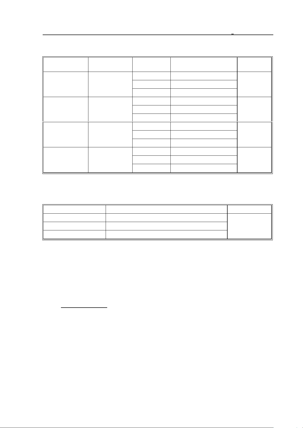
The value ranges of the length coordinates are shown in the Table below.
5 The Coordinate Data
input unit output unit increment
mm mm
inch mm
inch inch
mm inch
The value ranges of angular coordinates:
value range of length
system
IS-A ± 0.01-999999.99
IS-B ± 0.001-99999.999
IS-C ± 0.0001-9999.9999
IS-A ± 0.001-39370.078
IS-B ± 0.0001-3937.0078
IS-C ± 0.00001-393.70078
IS-A ± 0.001-99999.999
IS-B ± 0.0001-9999.9999
IS-C ± 0.00001-999.99999
IS-A ± 0.01-999999.99
IS-B ± 0.001-99999.999
IS-C ± 0.0001-9999.9999
coordinates
unit of
measure
mm
inch
inch
mm
increment system value range of angular coordinates unit of measure
IR-A ± 0.01-999999.99
IR-B ± 0.001-99999.999
IR-C ± 0.0001-9999.9999
degrees
5.5 Rotary Axis Roll-over
This function can be used in case of rotary axes, i.e., if address A, B or C is selected for operating
rotary axis. Handling of roll-over means, that the position on the given axis is not registered between
plus and minus infinity, but regarding the periodicity of the axis, e.g., between 0/ and 360/.
Selecting rotary axis
The selection can be executed by setting parameter 0182 A.ROTARY, 0185 B.ROTARY or 0188
C.ROTARY to 1 for axes A, B or C, respectively. If among these parameters one is set to 1
– the control does not execute inch/metric conversion for the appropriate axis,
– roll-over function can be enabled for that axis by setting the appropriate parameter ROLLOVEN
to 1.
41
Page 42
5 The Coordinate Data
Enabling the handling of roll-over
The function is affected by setting parameter 0241 ROLLOVEN_A, 0242 ROLLOVEN_B or
0243 ROLLOVEN_C to 1 for axes A, B or C, respectively, provided the appropriate axis is a
rotary one. If the given parameter ROLLOVEN_x
– =0: the rotary axis is regarded as linear axis and the setting of further parameters is uneffective,
– =1: handling of roll-over is applied for the rotary axis, the essence of which is discussed below.
Specifying path per roll-over
The path per one roll-over of the axis is defined at parameter 0261 ROLLAMNT_A, 0262
ROLLAMNT_B or 0263 ROLLAMNT_C in input increment for axes A, B or C, respectively.
Thus if the control is operating in increment system B and the axis rotates 360° per one roll-over,
the value to be written at the appropriate parameter is 360000.
With the help of the above parameter settings the control always displays the position of the rotary
axis in range 0°- +359.999° independent of the direction of rotation and the number of revolutions.
Movement of rotary axis in case of absolute programming
In case of absolute data input, when handling of roll-over is enabled for rotary axis
(ROLLOVEN_x=1), the axis never moves more than that set at appropriate parameter
ROLLAMNT_x. That is, if, e.g., ROLLAMNT_C=360000 (360/), the maximum movement is
359.999°.
For the movement direction to always be according to the sign of position given at the axis address
or in the shorter way can be set on the basis of parameter 0244 ABSHORT _A, 0245
ABSHORT_B or 0246 ABSHORT_C. If appropriate parameter ABSHORT_x
– =0: it always moves in the direction of the sign of the programmed position
– =1: it always moves in the shorter direction.
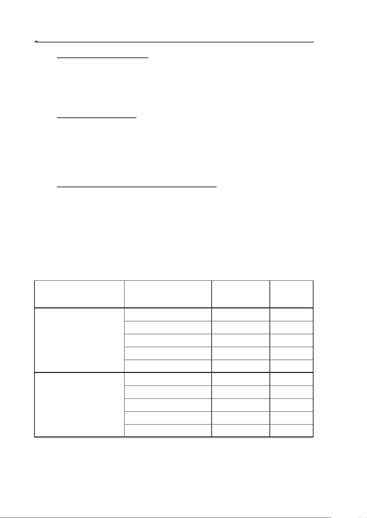
0188 C.ROTARY=1,
0243 ROLLOVEN_C=1
0263 ROLLAMNT_C = =360000
0246 ABSHORT_C=0
it always moves in direction of
sign programmed at address C
0246 ABSHORT_C=1
it always moves in the shorter
direction
Block programmed by absolute
coordinate input
G90 C450 90 C=90
G90 C0 (0 is a positive number!) 270 C=0
G90 C–90 –90 C=270
G90 C–360 –270 C=0
G90 C450 90 C=90
G90 C0 –90 C=0
G90 C–90 –90 C=270
G90 C–360 90 C=0
Movement affected
by block
Position at
block end
C=0
C=0
42
Page 43
5 The Coordinate Data
Movement of rotary axis in case of incremental programming
In case of programming incremental data input the direction of movement is always according to the
programmed sign.
The appropriate parameter ROLLAMNT_x to be applied for movement setting can be set at
parameter 0247 RELROUND_A, 0248 RELROUND_B or 0249 RELROUND_C for axis A, B
or C, respectively. If the appropriate parameter RELROUND_x
– =0: parameter ROLLAMNT_x is out of use, i.e. the movement can be greater than 360/,
– =1: parameter ROLLAMNT_x is in use. If, e.g., ROLLAMNT_C=360000 (360/), the largest
movement on axis C may be 359.999°.
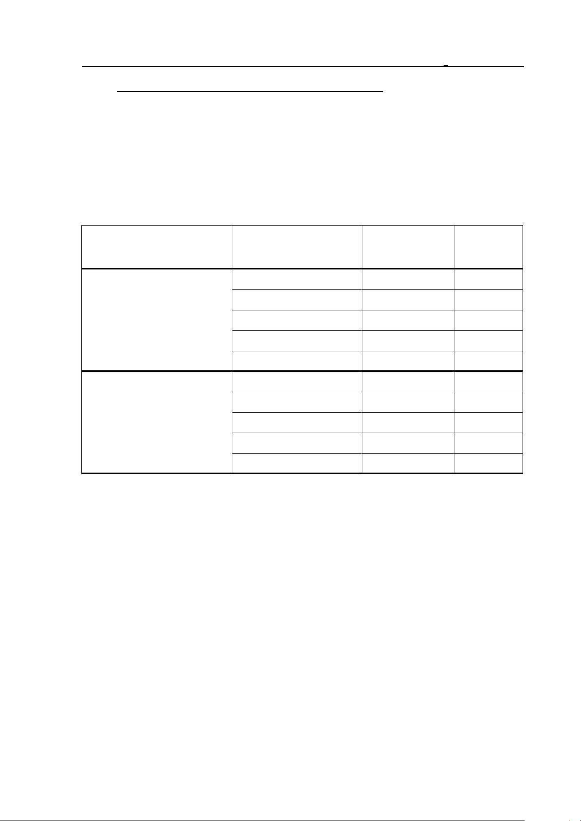
0188 C.ROTARY=1,
0243 ROLLOVEN_C=1
0263 ROLLAMNT_C = =360000
0249 RELROUND_C=0
parameter ROLLAMNT_C is out of
use
0249 RELROUND_C=1
parameter ROLLAMNT_C is in use
Block programmed by
incremental data input
G91 C450 450 C=90
G91 C0 0 C=90
G91 C–90 –90 C=0
G91 C–360 –360 C=0
G91 C450 90 C=90
G91 C0 0 C=90
G91 C–90 –90 C=0
G91 C–360 0 C=0
Movement affected
by block
Position at
block end
C=0
C=0
43
Page 44
6 The Feed
6 The Feed
6.1 Feed in rapid travers
G00 commands a positioning in rapid traverse.
The value of rapid traverse for each axis is set by parameter by the builder of the machine. The rapid
traverse may be different for each axis.
When several axes are performing rapid traverse motions simultaneously, the resultant feed will be
calculated in such a way that the speed component of each axis will not exceed the particular rapid
traverse value (set as a parameter), and the positioning is accomplished in a minimum of time.
Rapid traverse rate is modified by the rapid traverse override switch that can be
F0: defined by parameter RAPOVER in %,
and 25%, 50%, 100%.
The rapid traverse rate will not exceed 100%.
Rapid traverse will be stopped if the state of the feedrate override switch is 0%.
In lack of a valid reference point, the reduced rapid traverses defined by the machine tool builder by
parameter will be effective for each axis until the reference point is returned.
Rapid traverse override values can be connected to the feedrate override switch.
When the slide is being moved by the jog keys, the speed of rapid traverse is different from the
rapid traverse in G00, it is also selected by parameters separately for each axis. Appropriately it is
lower than the speed of positioning for human response times.
6.2 Cutting Feed Rate
The feed is programmed at
address F.
The programmed feed is
accomplished in blocks of
linear (G01) and circular
interpolations (G02, G03).
The feed is accomplished
tangentially along the programmed path.
Fig. 6.2-1
F - tangential feed (programmed value)
Fx - feed component in the X direction
Fy - feed component in the Y direction
Except for override and stop inhibit states (G63), the programmed feed can be modified over the
range of 0 to 120% with the feed-override switch.
44
Page 45

6 The Feed
The feed value (F) is modal. After power-on, the feed value set at parameter FEED will be
effective.
6.2.1 Feed per Minute (G94) and Feed per Revolution (G95)
The unit of feed can be specified in the program with the G94 and G95 codes:
G94: feed per minute
G95: feed per revolution
The term "feed/minute" refers to a feed specified in units mm/minute, inch/minute or degree/minute.
The term "feed/rev" refers to the feed accomplished in a revolution of the spindle, in units of mm/rev,
inch/minute or deg/rev. A G95 cannot be programmed unless the spindle is equipped with an
encoder.
Modal values. After power-on, state G94 or G95 will be selected with reference to parameter
group CODES. State G94/G95 will be unaffected the rapid traverse, it is invariably in units of
minutes.
45
Page 46
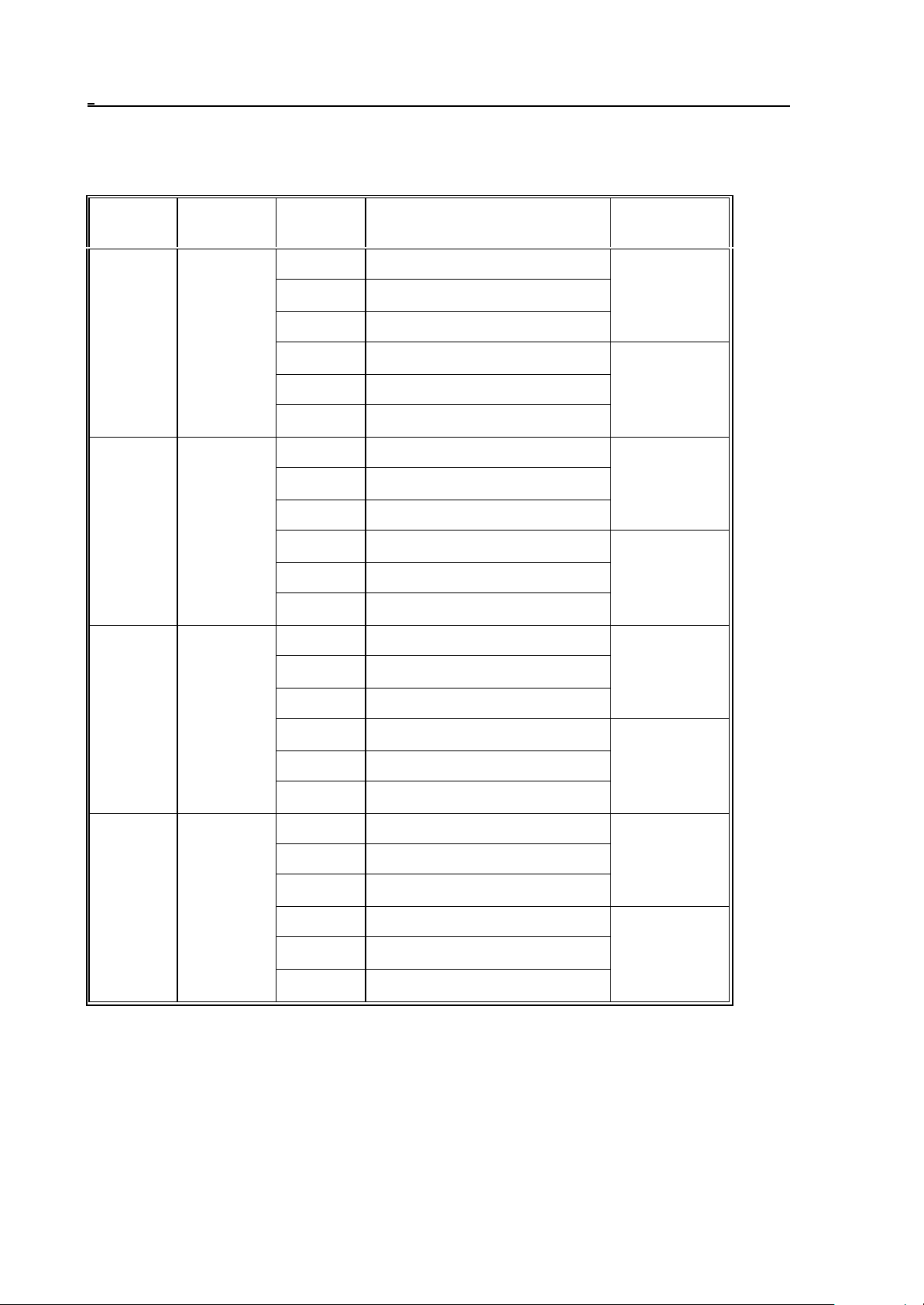
6 The Feed
The Table below shows the maximum programmable range of values at address F, for various
cases.
input
units
mm mm
inch mm
inch inch
output
units
increment
system
IS-A 0.001 - 250000 mm
IS-B 0.0001 - 25000
IS-C 0.00001 - 2500
IS-A 0.0001 - 5000 mm
IS-B 0.00001 - 500
IS-C 0.000001 - 50
IS-A 0.0001 - 9842.5197 inch
IS-B 0.00001 - 984.25197
IS-C 0.000001 - 98.25197
IS-A 0.00001 - 196.85039 inch
IS-B 0.000001 - 19.685039
IS-C 0.0000001 - 1.9685039
IS-A 0.0001 - 25000 inch
IS-B 0.00001 - 2500
IS-C 0.000001 - 250
IS-A 0.00001 - 500 inch
IS-B 0.000001 - 50
IS-C 0.0000001 - 5
value range of address F unit
or
deg/min
or
deg/rev
or
deg/min
or
deg/rev
or
deg/min
or
deg/rev
IS-A 0.001 - 250000 mm
or
deg/min
or
deg/rev
mm inch
IS-B 0.0001-25000
IS-C 0.00001-2500
IS-A 0.0001 - 5000 mm
IS-B 0.00001-500
IS-C 0.000001-50
6.2.2 Clamping the Cutting Feed
The maximum programmable feed on a particular machine can be clamped (set as a parameter) by
the manufacturer of the machine. The value set there invariably refers to minutes. That value is also
the speed of DRY RUN. If a programmed feed higher than that is set, the control will clamp it
46
Page 47
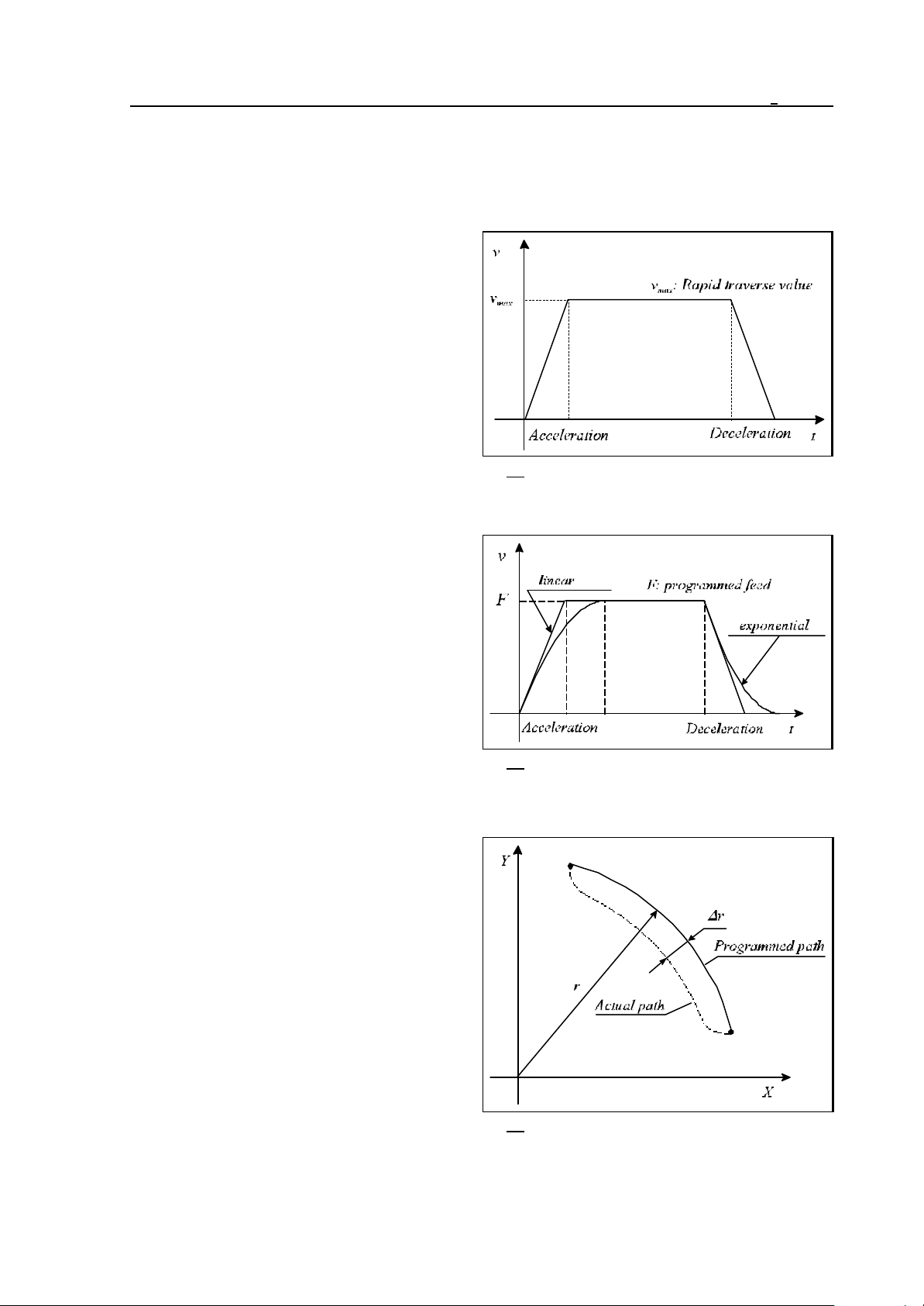
6 The Feed
automatically in the course of program execution.
The maximum jog feed can also be clamped separately by parameters for human response times.
6.3 Automatic Acceleration/Deceleration
In rapid traverse, the control will automatically
perform a linear acceleration and linear
deceleration when starting and ending a
movement. The extent of acceleration is defined
by the machine tool builder, in parameter
ACCn, depending on the dynamics of the
machine.
Fig. 6.3-1
In feed motions the tangential (programmed)
feed value will be assumed by the control in
linear acceleration, inversely, its value will be
decreased by linear deceleration. This
technique offers the advantage over traditional
(exponential) accelerations that the machine will
sooner attain the desired speed (assuming a
given time constant adopted in both cases).
Thus the times of acceleration and deceleration
(i.e., the times of actual slide movements) will be
reduced.
Another advantage of linear acceleration over
the exponential one is the lower profile
distortion (i.e., radius error), compared with
exponential acceleration, in a high-speed
machining of a circle.
Fig. 6.3-2
Fig. 6.3-3
47
Page 48
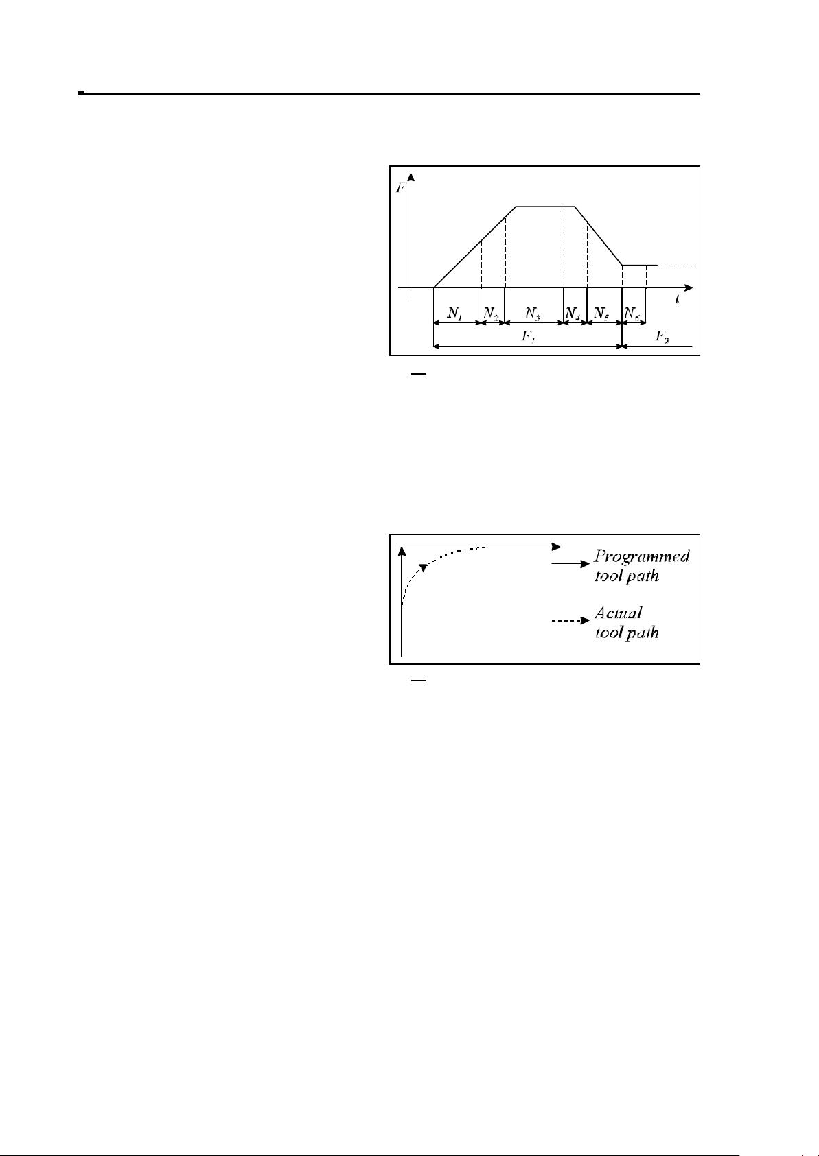
6 The Feed
The control is monitoring the changes in tangential speeds. This is necessary to attain the
commanded speed in a process of continuous acceleration, if necessary, through several blocks. The
acceleration to the new feed (higher than the
previous one) is commenced by the control
invariably in the execution of the particular
block, in which the new feed value is specified.
That process may, if necessary, cover several
blocks. Deceleration to the new feed value
(lower than the previous one) will be started by
the control in an appropriate preceding block so
that the machining will be started with the
programmed speed in the particular block, in
which the new feed value is specified.
Fig. 6.3-4
When moving manually by using jog keys or
handwheel, again linear acceleration/deceleration will be performed. Their values will be defined for
each axis by parameters ACC1 through ACC8.
6.4 Feed Control Functions
The override control functions are required when corners are to be machined, and/or when the
particular technology requires the override and stop switches to be canceled.
When machining corners, with continuous
cutting applied, the slides are - on account of
their inertia - unable to follow the path
commanded by the control system. Now the
tool will round the corner more or less,
depending on the feed.
If the workpiece requires sharp corners, the
Fig. 6.4-1
control must be specified to slow down at the
end of block, wait until the axes come to a halt, and start the next movement only afterwards.
6.4.1 Exact Stop (G09)
Not being a modal function, G09 will be effective only in the block, in which it has been
programmed.
At the end of the block, it has been specified, the control will slow down after execution of the
interpolation, and will wait for the "in position" signal. Unless that signal arrives in 5 seconds, the
control will return a message 1020 POSITION ERROR.
That function can be used for exact machining sharp corners.
6.4.2 Exact Stop Mode (G61)
Modal function, canceled with G62, G63 or G64 command.
The control system will slow on completion of each interpolation and wait for the "in position" signal.
It will start the next interpolation cycle only afterwards. Unless that signal arrives in 5 seconds, the
control will return a message 1020 POSITION ERROR.
48
Page 49
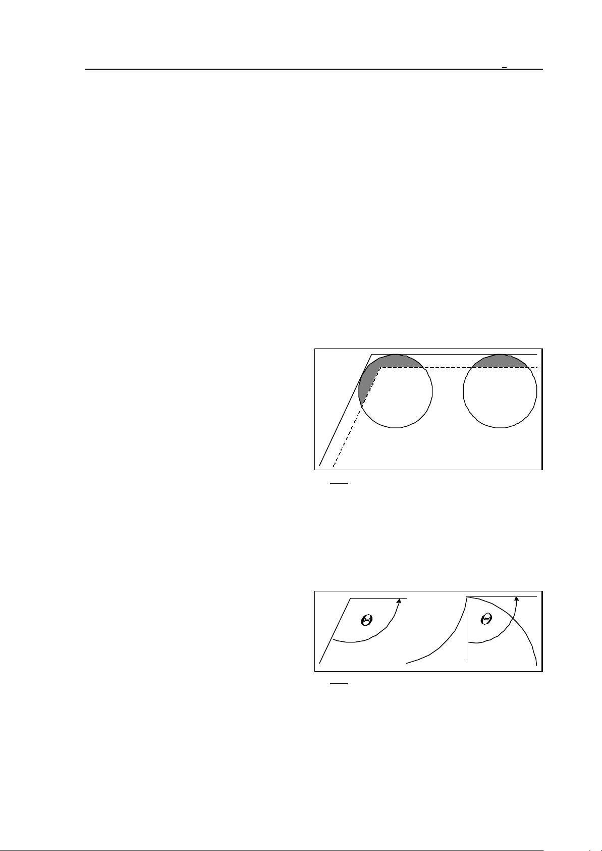
6 The Feed
6.4.3 Continuous Cutting Mode (G64)
Modal function. The control will assume that state after power-on. It will be canceled by codes
G61, G62 or G63.
In this mode the movement will not come to a halt on the completion of the interpolation, the slides
will not slow down. Instead, the interpolation of the next block will be commenced immediately.
Sharp corners cannot be machined in this mode, because they will be rounded off.
6.4.4 Override and Stop Inhibit (Tapping) Mode (G63)
Modal function, canceled by codes G61, G62 or G64.
The feed and spindle override and the feed stop is inhibited in this mode. The override values are
taken for 100% (regardless of switch positions). On completion of the interpolation, the system will
not slow down, but start next interpolation cycle immediately.
This mode is applicable in various thread cutting and tapping operations.
6.4.5 Automatic Corner Override (G62)
Modal function canceled by any of codes G61, G63 or G64.
When inside corners are being machined, higher
forces are acting upon the tool before and after
the corners. To prevent the overload of the tool
and developing vibrations, the control will when G62 commanded - automatically reduce
the feed along before and after an inside corner.
The corner override is effective under the
following conditions.
– When cutter compensation is on (G41, G42).
Fig. 6.4.5-1
– Between blocks G0, G1, G2, G3.
– In movements in the selected plane.
– When the corner is machined inside.
– When the angle of the corner is smaller then a particular angle defined by parameter.
– Over a distance before and after the corner, defined by parameters.
The corner override function will be effective between each the following pairs of blocks: linear-tolinear, linear-to-circular, circular-to-linear, circular-to-circular ones.
Inside angle 1 can be selected between 1 and
180° by parameter CORNANGLE.
Fig. 6.4.5-2
49
Page 50
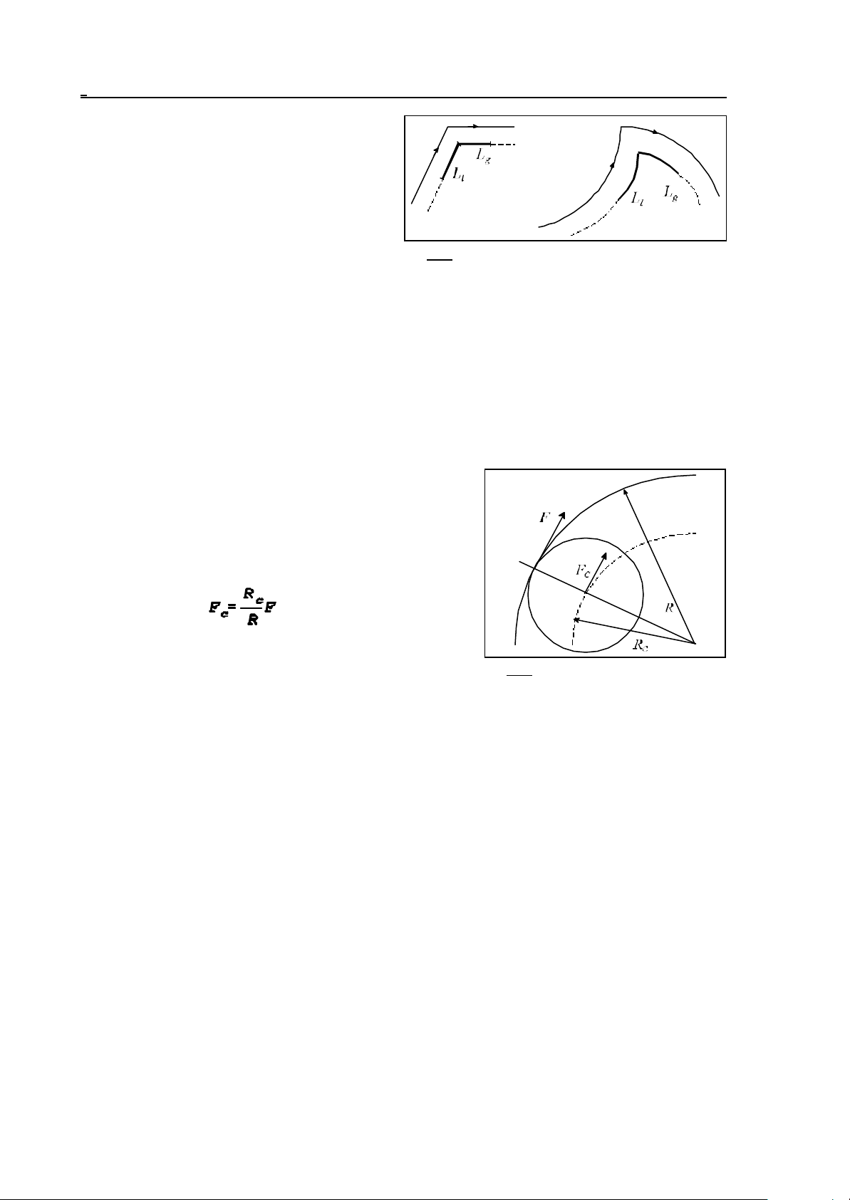
6 The Feed
Deceleration and acceleration will be
commenced at distances Ll and Lg before and
after the corner, respectively. In the case of
(circles) arcs, distance Ll and Lg will be
calculated by the control along the arc.
Distances Ll and Lg will be defined in
parameters DECDIST and ACCDIST,
Fig. 6.4.5-3
respectively.
The value of override can be selected as a percent in parameter CORNOVER. The override will
begin to be effective at distance Ll before the corner, and will be effective over distance Lg behind
the corner. The values of feed override and corner override will be taken into account together by
the control:
F* feed override * corner override.
Write G09 in the particular block to program an exact stop in state G62.
6.4.6 Internal Circular Cutting Override
With the cutter compensation on (G41, G42), the control
will automatically reduce the feed in machining the inside
surface of an arc so that the programmed feed will be
effective along the cutting radius. The feed in the center of
the tool radius is
where Fc is the (corrected) feed of the tool-radius center
Fig. 6.4.6-1
R is the programmed radius of circle
Rc is the corrected radius of circle
F is the programmed feed.
The lower limit of automatic feed reduction is set by parameter CIRCOVER, in which the minimum
override can be specified as a percent. The override for the circle radius is multiplied by the values
of feed and corner override before it is issued.
50
Page 51

7 The Dwell
7 The Dwell (G04)
The
(G94) G04 P....
command will program the dwell in seconds.
The range of P is 0.001 to 99999.999 seconds.
The
(G95) G04 P....
command will program the dwell in terms of spindle revolutions.
The range of P is 0.001 to 99999.999 revolutions.
Depending on parameter SECOND, the delay may refer always to seconds as well, irrespective of
the states of G94, G95.
The dwell implies invariably the programmed delay of the execution of the next block. It is a nonmodal function.
During dwell in status field 5 indicating interpolation status the message DWL will appear on screen
to draw the attention of operator why the machine is halted.
51
Page 52
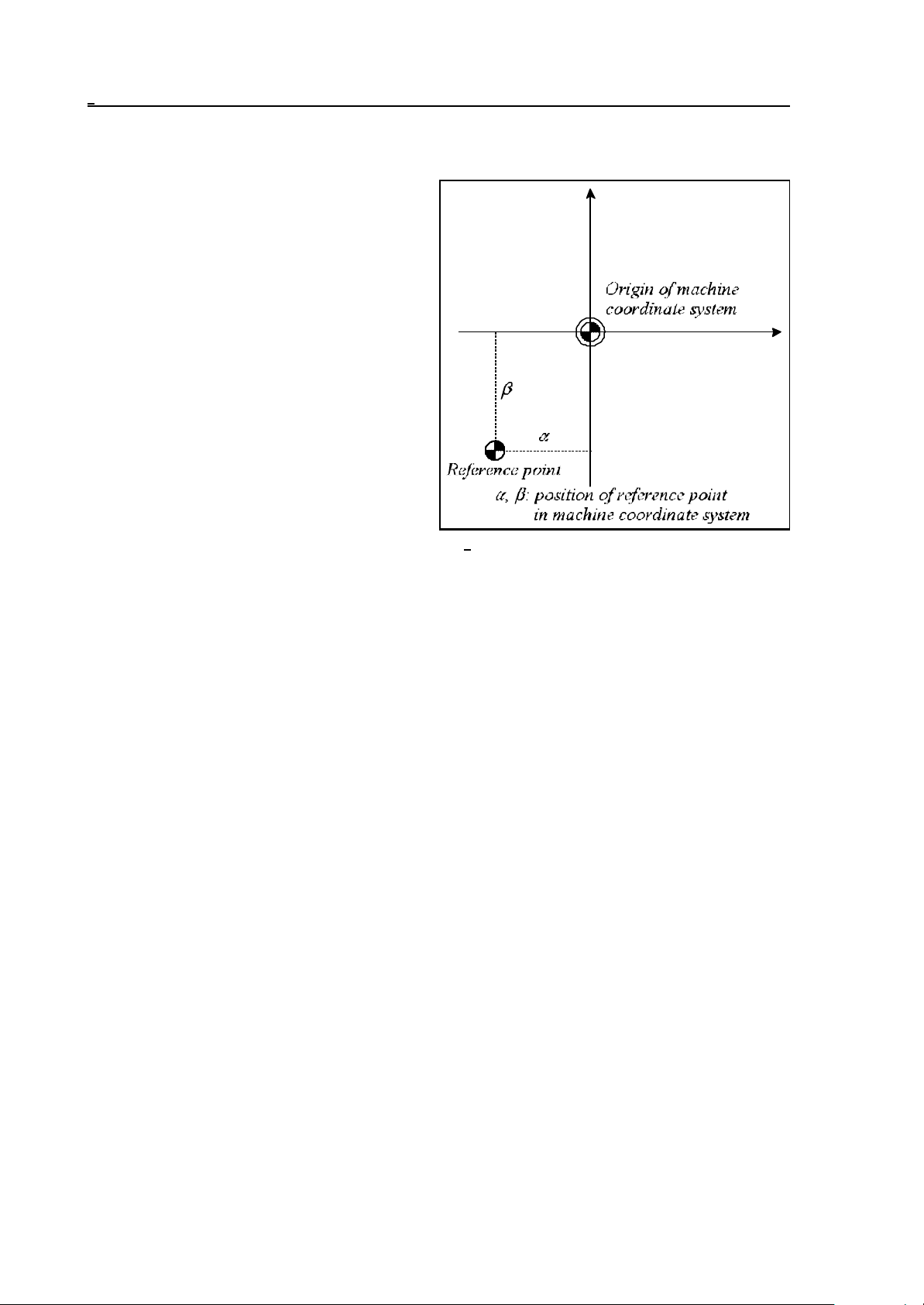
8 The Reference Point
8 The Reference Point
The reference point is a distinguished position
on the machine-tool, to which the control can
easily return. The location of the reference point
can be defined as a parameter in the coordinate
system of the machine. Work coordinate system
can be measured and absolute positioning can
be done after reference point return. The
parametric overtravel positions and the stroke
check function are only effective after
reference-point return.
Fig. 8-1
8.1 Automatic Reference Point Return (G28)
The instruction
G28 v
will return the axes defined by vector v to the reference point. The movements consist of two parts.
First it will move with linear interpolation in rapid traverse to the intermediate coordinates defined by
vector v. The specified coordinates may be absolute or incremental values. The movement is
performed invariably in the current coordinate system .
When the end point of linear movement is reached, the cutter compensation vector is deleted.
The coordinates of the intermediate point will be stored for axes defined by vector v.
In the second stage it will move from the intermediate point to the reference-point simultaneously in
each axis defined by vector v. The reference-point return is carried out by non-linear movement at a
speed defined for each axis. Afterwards, similar to the manual return, the position will be assumed in
the manner defined by parameters.
This is a non-modal code.
L Notes:
– Unless there is a valid reference point, incremental values must be assigned to intermediate
coordinates v in command G28.
– Programmed in block G28, intermediate coordinates v will be stored until power-off. In other
words, the intermediate value defined in a previous command G28 will continue to be effect
for the coordinates that have not been assigned values in the instantaneous (current)
command G28. For example:
G28 X100 intermediate point: X=100, Y=0
G28 Y200 intermediate point: X=100, Y=200
52
Page 53

8 The Reference Point
8.2 Automatic return to reference points 2nd, 3rd, 4th (G30)
Series of instructions
G30 v P
will send the axes of coordinates defined at the addresses of vector v to the reference point defined
at address P.
P1=reference point 1
P2=reference point 2
P3=reference point 3
P4=reference point 4
The reference points are special positions defined by parameters (REFPOS1, ..., REFPOS4) in the
coordinate system of the machine-tool, used for change positions, e.g., positions of tool change or
palette change. The first reference point is invariably the position of the machine's reference point,
i.e., the point to which the control moves when returning to the reference point.
The instruction is only applicable after the machine's reference point has been returned.
The movement consists of two parts. First it will move by a linear motion to the intermediate
coordinates defined by vector v, with rapid traverse. The specified coordinates may be absolute or
incremental values. The movement is carried out invariably in the current coordinate system. When
the end point of linear movement is reached, the cutter compensation vector will be deleted. The
coordinates of the intermediate point will be stored in the current coordinate system for the axes
defined by vector v. Stored in this way, the coordinates will overwrite those stored in instruction
G28.
In the second phase, the axes defined by vector v will move with rapid traverse from the
intermediate point to the reference point selected at address P.
The reference point is returned by disregarding the compensation vectors (length, offset, 3
dimensional offsets) they need not be deleted before instruction G30 is issued but they will be
implemented by the control when further movements are being programmed. The cutter
compensation is re-established automatically in the first movement block.
A non-modal code.
8.3 Automatic Return from the Reference Point (G29)
Instruction
G29 v
will return the control from the reference point along the axes defined in vector v. Following G28
and G30, command G29 will be executed in the same manner. The return is accomplished in two
stages.
In the first stage it will move from the reference point to the intermediate point recorded during the
execution of instruction G28 or G30, in the axes defined by vector v. The coordinates of the
intermediate point are modal, in other words, the control will take the previous values into account if
reference is made to an axis, to which no coordinate has been transferred in block G28 or G30
preceding G29. It will move to the intermediate point by taking into account the tool length, tool
offset and 3-dimensional tool radius compensations.
The coordinates of the intermediary point are effective invariably in the coordinate system of the
current workpiece. Accordingly if, e.g., a change of workpiece coordinate system has been
programmed after reference point return and before instruction G29, the intermediate point will be
53
Page 54
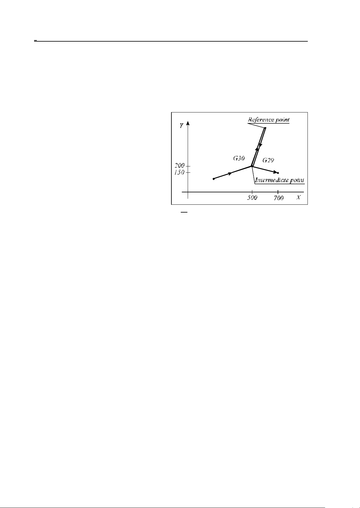
8 The Reference Point
taken into account in the new coordinate system.
In the second phase it will move from the intermediate point to the point v defined in instruction G29.
If coordinate v has an incremental value, the displacement will be measured from the intermediate
point.
When the cutter compensation is set up, it will move to the end point by taking into account the
compensation vector.
A non-modal code.
An example of using G30 and G29:
...
G90
...
G30 P1 X500 Y200
G29 X700 Y150
...
...
Fig. 8.3-1
54
Page 55
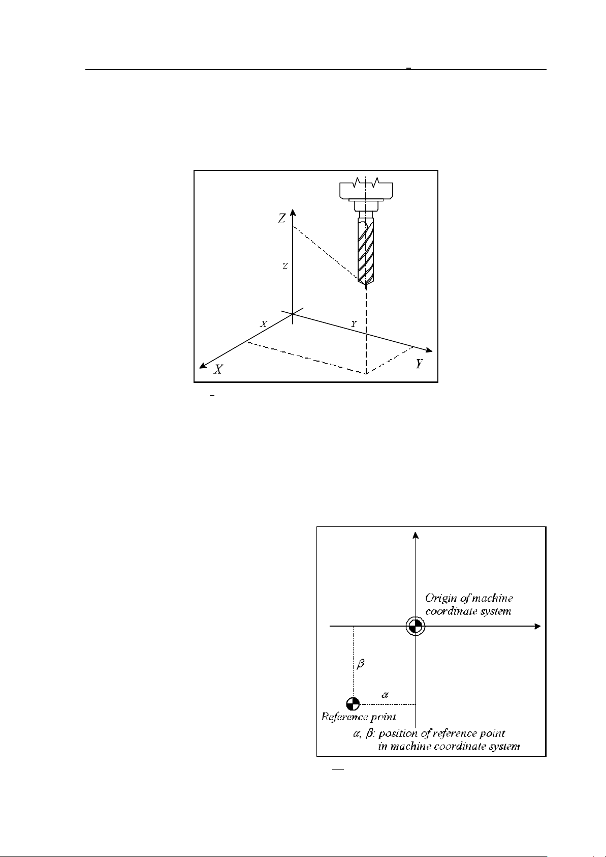
9 Coordinate Systems, Plane Selection
9 Coordinate Systems, Plane Selection
The position, to which the tool is to be moved, is specified with coordinate data in the program.
When 3 axes are available (X, Y, Z), the position of the tool is expressed by three coordinate data
X____ Y____ Z____ :
Fig. 9-1
The tool position is expressed by as many different coordinate data as is the number of axes on the
machine. The coordinate data refer invariably to a given coordinate system.
The control will differentiate three different coordinate systems.
1. the machine coordinate system,
2. the workpiece's coordinate system,
3. the local coordinate system.
9.1 The Machine Coordinate System
The machine zero point, i.e., the origin of the
machine coordinate system, is a point on the
given machine-tool, that is usually defined by the
machine tool builder. The control will define the
machine coordinate system at the time of
returning to the reference point.
Once the machine coordinate system has been
defined, it will not be altered by the change of
the work coordinate system (G54 ... G59) or
by other coordinate transformation (G52, G92),
only by a power-off of the control system.
Fig. 9.1-1
55
Page 56
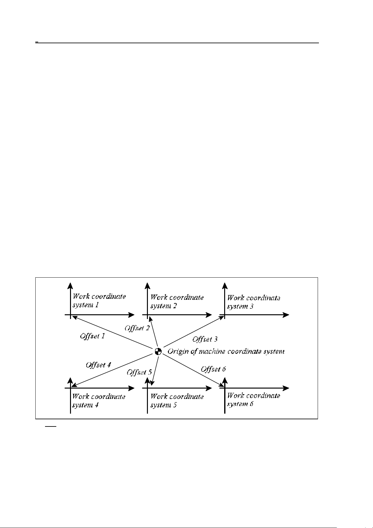
9 Coordinate Systems, Plane Selection
9.1.1 Setting the Machine Coordinate system
After a reference point return, the machine coordinate system can be set in parameters. The distance
of the reference point, calculated from the origin of the machine coordinate system, has to be written
for the parameter.
9.1.2 Positioning in the Machine Coordinate System (G53)
Instruction
G53 v
will move the tool to the position of v coordinate in the machine coordinate system.
– Regardless of states G90, G91, coordinates v are always treated as absolute coordinates,
– operator I is ineffective when put behind the address of a coordinate,
– similar to instruction G00, the movements are performed in rapid traverse,
– the positioning is carried out invariably with the selected tool length compensations taken into
account.
A G53 instruction can be executed after a reference point return only. G53 is a one-shot command
effective in the block only, where it has been specified.
9.2 Work Coordinate Systems
The coordinate system applied in cutting the workpiece is referred to as the "work coordinate
system". Six different coordinate systems can be defined for the workpiece in the control.
9.2.1 Setting the Work Coordinate Systems
Fig. 9.2.1-1
In setting mode the locations of the various work coordinate systems can be established in the
machine coordinate system, and the necessary offsets can be made.
56
Page 57
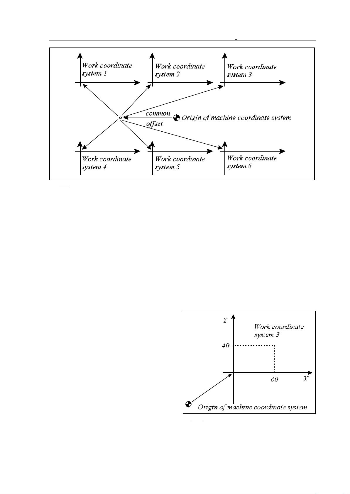
9 Coordinate Systems, Plane Selection
Fig. 9.2.1-2
Furthermore, all work coordinate system can be offset with a common value. It can also be entered
in setting mode.
9.2.2 Selecting the Work Coordinate System
The various work coordinate system can be selected with instructions G54...G59.
G54........work coordinate system 1
G55........work coordinate system 2
G56........work coordinate system 3
G57........work coordinate system 4
G58........work coordinate system 5
G59........work coordinate system 6
They are modal functions. Their selection before a reference point return is ineffective. After a
reference point return, work coordinate system
1 (G54) will be selected.
The absolute coordinate data of the
interpolation blocks will be taken into account
by the control in the current work coordinate
system.
For example, the instruction
G56 G90 G00 X60 Y40
will move the system to point X=60, Y=40 of
work coordinate system 3.
Fig. 9.2.2-1
57
Page 58
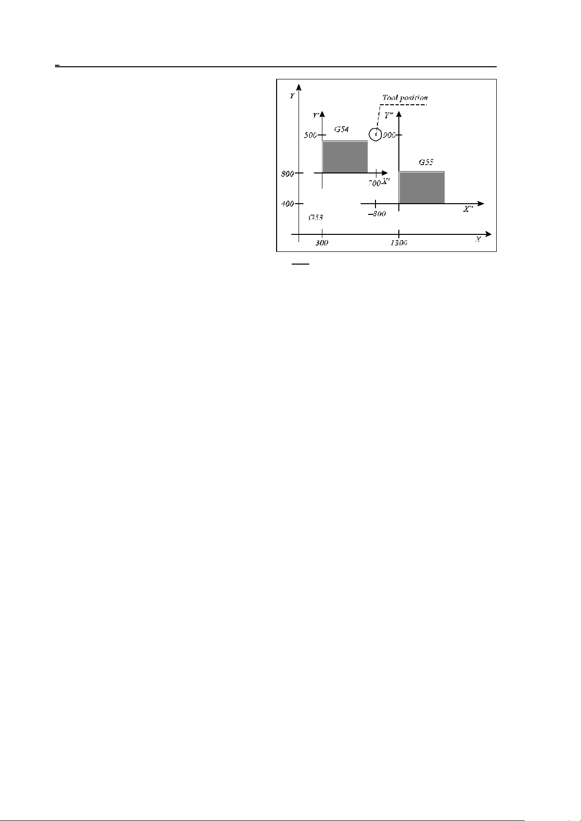
9 Coordinate Systems, Plane Selection
After a change of the work coordinate system,
the tool position will be displayed in the new
coordinate system. For instance, there are two
workpieces on the table. The first work
coordinate system (G54) has been assigned to
zero point of one of the workpieces, which has
an offset of X=300, Y=800 (calculated in the
machine coordinate system). The second work
coordinate system (G55) has been assigned to
the zero point of the other workpiece, which has
an offset of X=1300, Y=400 (calculated in the
machine coordinate system). The tool position is
X'=700, Y'=500 in X', Y's’ coordinate system
Fig. 9.2.2-2
(G54). As a result of instruction G55, the tool position will be interpreted in the X", Y" coordinate
system (X"=-300, Y"=900).
9.2.3 Programmed Setting of the Work Zero Point Offset
It is also programable to set the work coordinate system and the common offset thereof with
program instructions.
This is accomplished with instruction
G10 v L2 Pp
where
p = 0 sets the common offset,
p = 1...6 selecting work coordinate system 1.- 6.
v = offset for each axis.
The coordinate data are entered invariably as rectangular (Cartesian) absolute values. G10 is a one-
shot (non-modal) instruction.
9.2.4 Creating a New Work Coordinate System (G92)
Instruction
G92 v
will establish a new work coordinate system in such a way that coordinate point v of the new system
will be a selected point - e.g. the tool's tip (if a length compensation is programmed) or the base
point of the tool holder (in lack of a length compensation). Afterwards any additional absolute
command will refer to that new work coordinate system, and the positions will also be displayed in
that coordinate system. The coordinates specified in command G92 will always be interpreted as
rectangular absolute values.
58
Page 59
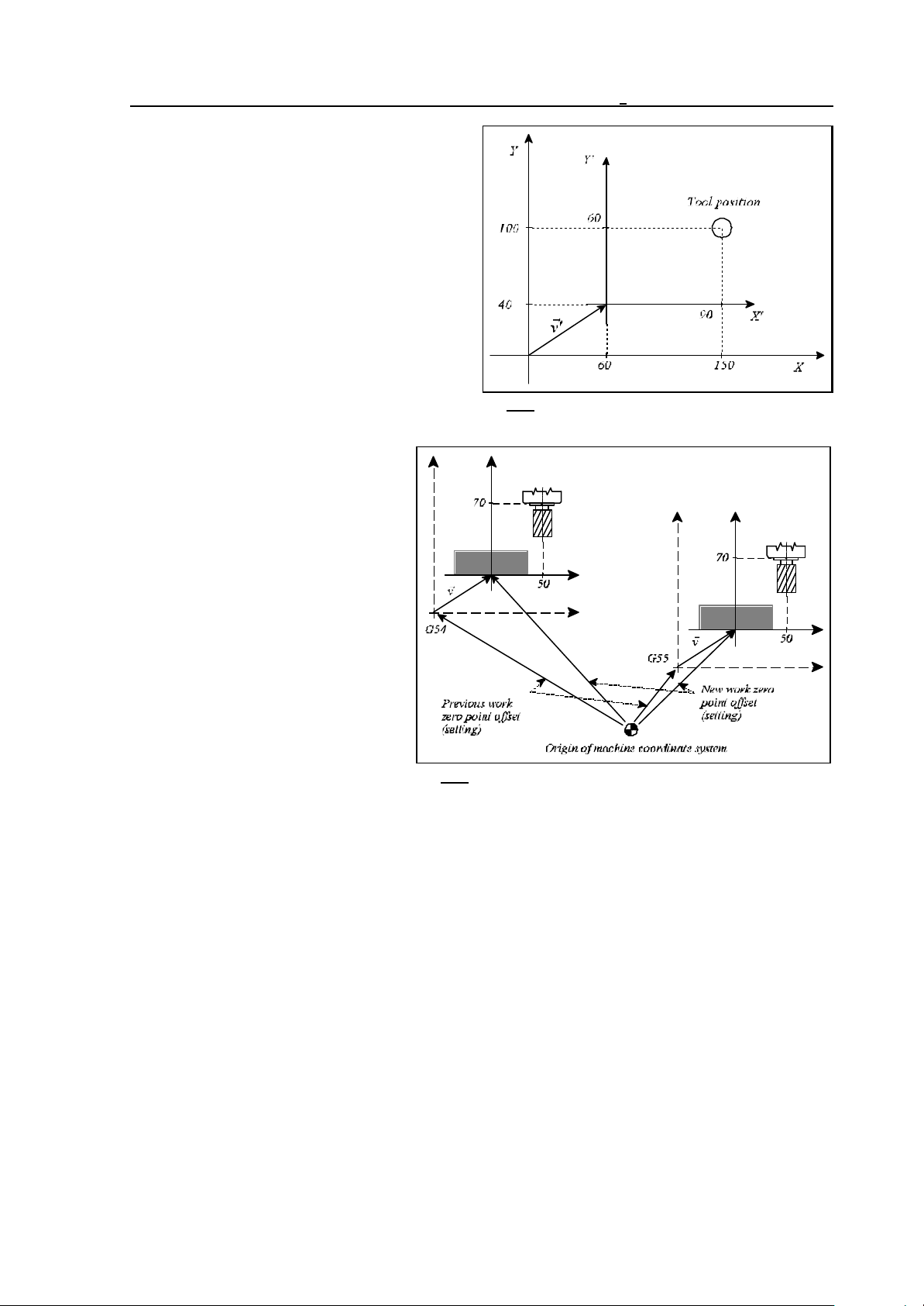
If, e.g., the tool is at a point of X=150, Y=100
coordinates, in the actual (current) X, Y work
coordinate system, instruction
G92 X90 Y60
will create a new X', Y' coordinate system, in
which the tool will be set to the point of X'=90,
Y'=60 coordinates. The axial components of
offset vector v' between coordinate systems X,
Y and X', Y' are
v'x=150-90=60,
and
v'y=100–60=40.
Command G92 will prevail in each of
the six work coordinate systems, i.e.,
an offset v calculated for one of them
will be taken into account in the rest,
too.
9 Coordinate Systems, Plane Selection
Fig. 9.2.4-1
Fig. 9.2.4-2
L Notes:
– The offset of the work coordinate system set with instruction G92 will be deleted by execution of
"end of program" instructions (M2, M30) and by resetting the program.
– Instruction G92 will delete the offsets of the local coordinate system (programmed with instruction
G52) on the axes included in the instruction.
– Instruction G92 offers a convenient way of the cyclic position indication of the indexing rotary
table performing several turns. If, e.g., axis B has been turned into the position 360°, the axis
can be moved to position 0° without any physical movement by programming G92 B0.
9.3 Local Coordinate System
When writing part programs, it is sometimes more convenient to specify the coordinate data in a
"local" coordinate system instead of the work part coordinate system.
Instruction
G52 v
59
Page 60
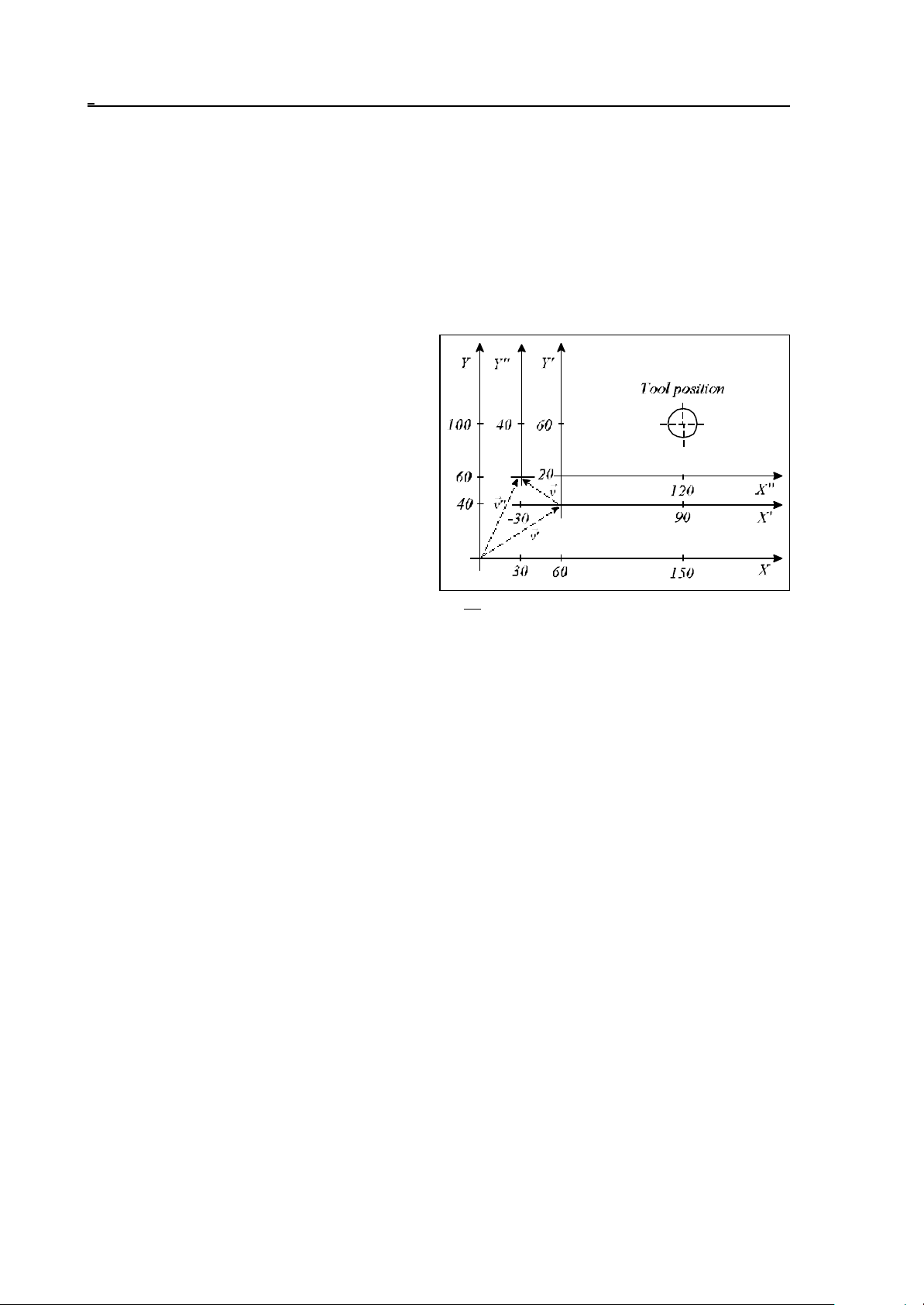
9 Coordinate Systems, Plane Selection
will create a local coordinate system.
– If coordinate v is specified as an absolute value, the origin of the local coordinate system will
coincide with the point v in the work coordinate system.
– When specified as an incremental value, the origin of the local coordinate system will be shifted
with v offset (provided a local coordinate system has been defined previously, or else the
offset is produced with respect to the origin of the work coordinate system).
Henceforth any movement command specified in absolute coordinates will be executed in the new
coordinate system. The positions are also displayed in the new coordinate system. The values of
coordinates v will be treated invariably as Cartesian coordinates.
If, e.g., the tool is at point X=150, Y=100
coordinates in the current X, Y work coordinate
system, instruction
G90 G52 X60 Y40
will create a new local X', Y' coordinate
system, in which the coordinates of tool will be
X'=90, Y'=60. Instruction G52 is used for
defining the axial components of offset vector v'
between the X, Y and X', Y' coordinate
systems (v'x=60, v'y=40).
Now one of two different procedures may be
adopted in order to transfer the local coordinate
Fig. 9.3-1
system to the point of X", Y" position.
– With an absolute data specification: instruction (G90) G52 X30 Y60 will move the origin of the
X", Y" coordinate system to point X=30, Y=60 in the X,Y work coordinate system. The
components of vector v" will be produced by the specification of v"x=30, v"y=60.
– With an incremental data specification: instruction G91 G52 X-30 Y20 will move the origin of the
X", Y" coordinate system to the point of X'=-30, Y'=20 coordinates in the X', Y' coordinate
system. The components of vector v will be produced by the specification of vx=-30, vy=20.
Indicating the location of the new local coordinate system in the X, Y work coordinate
system vector v"=v'+v. Its components:
v"x=60+(-30)=30, v"y=40+20=60.
The tool position in the X", Y" coordinate system will be X"=90, Y"=40.
Instruction
G90 G52 v0
will delete the offset in on coordinates specified in v.
60
Page 61
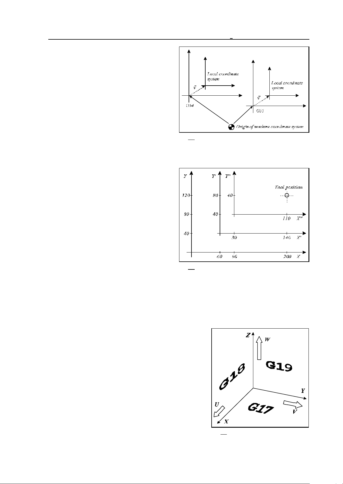
9 Coordinate Systems, Plane Selection
The local coordinate system will be offset in
each work coordinate system.
Fig. 9.3-2
Programming instruction G92 will delete the offsets produced by instruction G52 on the axes
specified inG92 - as if command G52 v0 had been issued.
Whenever the tool is at point of X=200, Y=120
coordinates in the X, Y work coordinate
system, instruction
G52 X60 Y40
will shift its position to X'=140, Y'=80 in the X',
Y' local coordinate system.
Now instruction
G92 X110 Y40
will establish the tool position to X"=110,
Y"=40 in the new X", Y" work coordinate
system. Thus the X', Y' local coordinate system
will be deleted by command G92 as if
Fig. 9.3-3
command G52 X0 Y0 had been issued.
L Note:
– The offset of the local coordinate system will be deleted by execution of commands M2, M30
and/or by resetting the program.
9.4 Plane Selection (G17, G18, G19)
The plane in which
– circular interpolation,
– specification of polar coordinate data,
– rotation of coordinate system,
–cutter radius compensation,
– positioning of drilling cycles
will be performed can be selected with the following G
codes:
G17............XpYp plane
G18............ZpXp plane
G19............YpZp plane,
where
Fig. 9.4-1
61
Page 62

9 Coordinate Systems, Plane Selection
Xp=X or an axis parallel to X,
Yp=Y or an axis parallel to Y,
Zp=Z or an axis parallel to Z.
The selected plane is referred to as "main plane".
The particular one of the parallel axes will be selected (by instruction G17, G18 or G19) depending
on the axis addresses programmed in a given block:
When X and U, Y and V, Z and W are parallel axes:
the XY plane will be selected by G17 X_Y_,
the XV plane will be selected by G17 X_V_,
the UV plane will be selected by G17 U_V_,
the XW plane will be selected by G18 X_W_,
the YZ plane will be selected by G19 Y_Z_,
the VZ plane will be selected by G19 V_Z_.
Unless G17, G18, G19 is specified in a block, the selected plane remains unchanged:
G17 X____ Y____ plane XY
U____ Y____ plane XY remains.
Unless there is an axis address specified in the G17, G18, G19 block, the control will consider the
basic axes:
the XY plane will be selected by G17,
the XY plane will be selected by G17 X,
the UY plane will be selected by G17 U,
the XV plane will be selected by G17 V,
the ZX plane will be selected by G18,
the WX plane will be selected by G18 W.
The selected plane is unaffected by the movement command:
(G90) G17 G00 Z100
will select the XY plane, moving the Z axis to the point of coordinate 100.
After power-on, the default plane (G17 or G18) is specified according to the parameter group
CODES.
The main plane can be selected more times in the same program.
Address U, V, W can be selected as a parallel in parameters.
62
Page 63
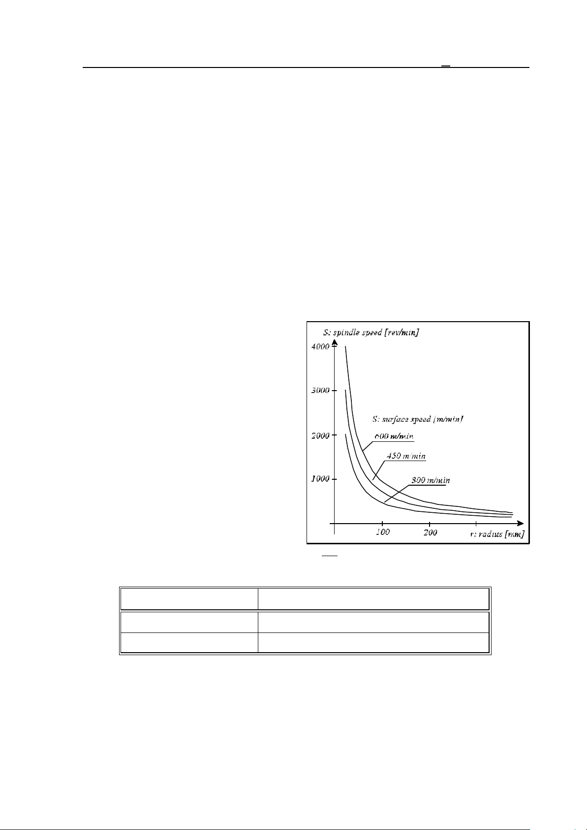
10 The Spindle Function
10 The Spindle Function
10.1 Spindle Speed Command (code S)
With a number of max. five digits written at address S, the NC will give a code to the PLC.
Depending on the design of the given machine-tool, the PLC may interpret address S as a code or
as a data of revs/minute.
When a movement command and a spindle speed (S) are programmed in a given block, function S
will be issued during or after the motion command. The machine tool builder will define the way of
execution.
The speeds specified at address S are modal values. At the time of power-on, the control will
assume value S0. The spindle speed has a minimum and a maximum limit in each gear ratio range.
They are defined by the machine-tool builder in parameters and the control does not let the speed
outside of this range.
10.2 Programming of Constant Surface Speed Control
Constant surface speed control function can
only be used in case of infinitely variable speed
main drive. In this case the control can change
the spindle speed so that the tool speed is
constant relative to the surface of the
workpiece and is equal to the programmed
value.
The constant surface speed must be specified
in function of the input unit on the basis of the
table below:
Fig. 10.2-1
Input unit Unit of constant surface speed
mm (G21 metric) m/min
inch (G20 inch) feet/min
63
Page 64

10 The Spindle Function
10.2.1Constant Surface Speed Control Command (G96, G97)
Command
G96 S
switches constant surface speed control function on. The constant surface speed must be specified
at address S in the unit of measure given in the above table.
Command
G97 S
cancels constant surface speed control. The desired spindle speed can be specified at address S (in
revs/min).
– In order to calculate constant surface speed the coordinate system must be set so that its zero
point coincides with the rotation axis.
– Constant surface speed control is effective only after the spindle is started by means of M3 or
M4.
– The value is modal even after its calculation has been canceled with the help of command G97.
After power on the default constant surface speed is determined by parameter CTSURFSP.
G96 S100 (100 m/min or 100 feet/min)
G97 S1500 (1500 revs/min)
G96 X260 (100 m/min or 100 feet/min)
– Constant surface speed calculation is also effective in state G94 (feed/min).
– If the constant surface speed control is canceled by means of command G97 and a new spindle
speed is not specified the last spindle speed gained in state G96 remains in effect.
G96 S100 (100m/min or 100 feet/min)
.
.
.
G97 (Revolution belonging to resulting diameter X)
– In case of rapid traverse positioning (block G00) the constant surface speed is not calculated
continuously but the revolution belonging to the end-position will be calculated. This is
needed for the spindle speed to avoid unnecessary changes.
– In order to calculate constant surface speed the zero point of the axis, on the basis the spindle
speed is changed, must be set to the spindle rotation axis.
10.2.2 Constant Surface Speed Clamp (G92)
With the help of command
G92 S
the highest spindle speed enabled in case of constant surface speed control can be set. During
constant surface speed calculation the control clamps spindle speed to this value. In this case the unit
of S is rpm.
– After power on as well as if value S has not been clamped by means of command G92 the top
limit of spindle speed in case of constant surface speed control is the maximum value
enabled for the given gear range.
– The maximum revolution value is modal until a new one is programmed or until the control is
turned off.
64
Page 65

10 The Spindle Function
10.2.3 Selecting an Axis for Constant Surface Speed Control
The axis, which position the constant surface speed is calculated from, is selected by parameter
1182 AXIS. The logic axis number must be written at the parameter.
If other than the selected axis is to be used, the axis from which the constant surface speed is to be
calculated can be specified by means of command
G96 P.
Interpretation of address P:
P1: X, P2: Y, P3: Z,
P4: U, P5: V, P6: W,
P7: A, P8: B, P9: C
– The value set at address P is modal. After power on the control activates constant surface speed
control to the axis set at parameter AXIS.
10.3 Spindle Position Feedback
In normal machining the NC will issue a speed command to the power amplifier of the spindle,
proportional to the programmed speed (value specified at address S). Now this amplifier will be
working in speed-control mode.
Some technological tasks may, however, require the spindle to be brought to a particular angular
position. This is referred to as spindle positioning or indexing.
Prior to positioning, the NC will set the power amplifier of the spindle to position-controlled mode.
In practice this means that the NC will not issue a speed command proportional to code S any
more, instead, it will measure the position of the spindle by the use of an encoder mounted on the
spindle, and will issue a command to the servo amplifier in accordance with the desired angular
displacement (similar to the rest of controlled axes). This is the position feedback.
To be able to position the spindle on a particular machine, an encoder has to be mounted on the
spindle and the power amplifier of the spindle must be capable of operation in position feedback
mode as well.
10.4 Oriented Spindle Stop
The "spindle orientation" or the "oriented spindle stop" refers to the function of stopping the spindle
in a particular angular position. This may be necessary, e.g., for an automatic tool change or for the
execution of some drilling cycles. The possibility of orientation on a particular machine must be
specified by parameter ORIENT1 in parameters. The command of spindle orientation is issued by
function M19, but it may also be produced by some other function depending on the particular
machine-tool. The orientation may be carried out in one of two different ways.
If the spindle cannot be used in position control mode, the orientation is feasible by turning the
spindle to a proximity switch mounted on the machine.
If the spindle can be used in position control mode, command M19 will cause the control to return
to the zero pulse of the spindle encoder. The control will automatically close the position control
loop.
65
Page 66
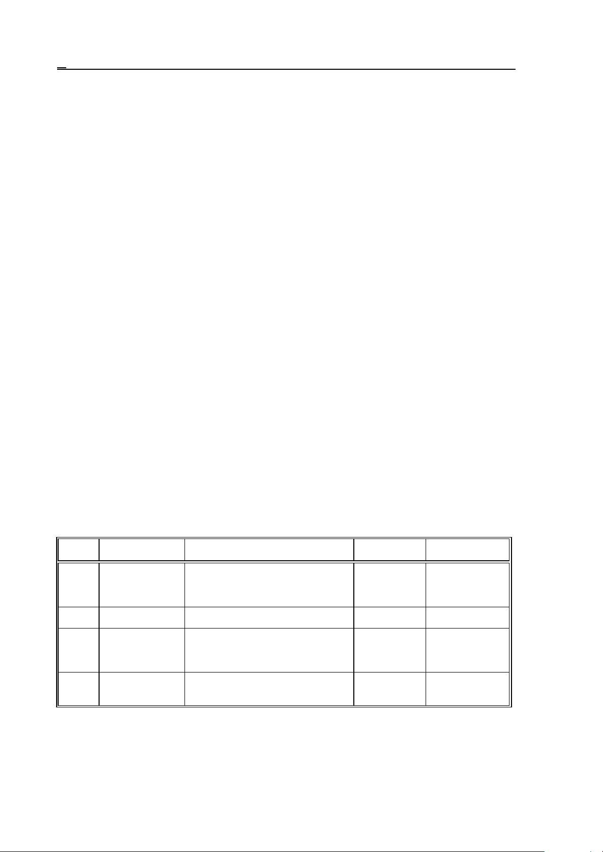
10 The Spindle Function
10.5 Spindle Positioning (Indexing)
A spindle positioning is only feasible after the spindle position control loop has been closed after
orientation. Accordingly, this function is used for closing the loop. The loop will be opened by
rotation command M3 or M4.
If the value of parameter INDEX1=1 (indicating that the main drive position control loop can be
closed) and the value of parameter INDEX_C1=0, the spindle indexing will be performed by
function M.
Under such conditions function M from the threshold value set on parameter M_NUMB1 to
M_NUMB1+360 will be interpreted as a spindle indexing commands, i.e., the threshold number will
be subtracted from the programmed value of M, and the number obtained will be treated as an
incremental displacement specified in degrees.
Thus, if M_NUMB1=100, command M160 means that the spindle must be turned by 160-100=60
degrees from its current position. The direction of rotation is selected by parameter CDIRS1, its rate
is selected by parameter RAPIDS1.
10.6 Spindle Speed Fluctuation Detection (G25, G26)
Command
G26
enables spindle speed fluctuation detection, while command
G25
cancels it. After power-on or RESET the control is set to state G26, i.e., spindle speed fluctuation
detection is on. This function signals abnormalities occurring in the course of spindle rotation, as the
result of which, e.g., spindle seizure can be avoided.
The speed fluctuation detection is influenced by 4 parameters. These parameters can be overwritten
from a program with addresses following command G26. The overwritten parameters are kept upon
power-off. The parameters are overwritten as the effect of command
G26 Pp Qq Rr Dd.
The below table contains the parameter interpretations:
name parameter meaning unit value limit
p 5001 TIME time from the issue of a new spindle
speed command to the start of
checking
q 5002 SCERR tolerance of a specified spindle speed % 1-50
r 5003 FLUCT% allowable amount of spindle speed
fluctuation in the percentage of
programmed speed
d 5004 FLUCTW spindle speed fluctuation in absolute
value
100 msec 65535
% 1-50
revs/min 65535
The process of speed fluctuation detection is as follows.
66
Page 67
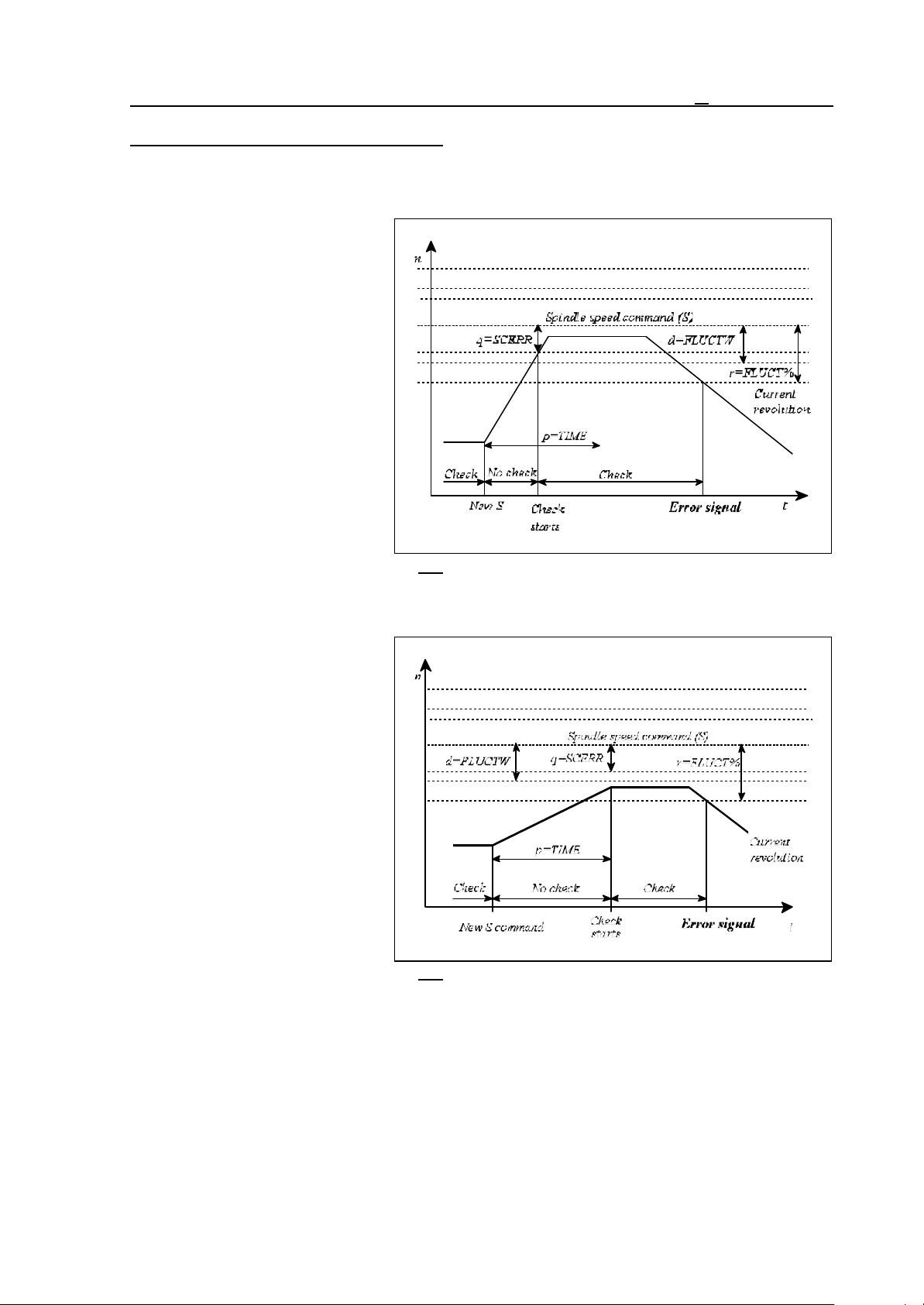
10 The Spindle Function
Start of Spindle Speed Fluctuation Detection
As the effect of new rotation speed the detection is suspended by the control. The speed fluctuation
detection starts when
- the current spindle speed
reaches the specified spindle
speed within the tolerance limit
determined by value "q", or
- the current spindle speed has
not reached the specified spindle
speed within the tolerance limit
determined by value "q", but time
determined by value "p" has
elapsed from the command .
Fig. 10.6-1
Fig. 10.6-2
67
Page 68
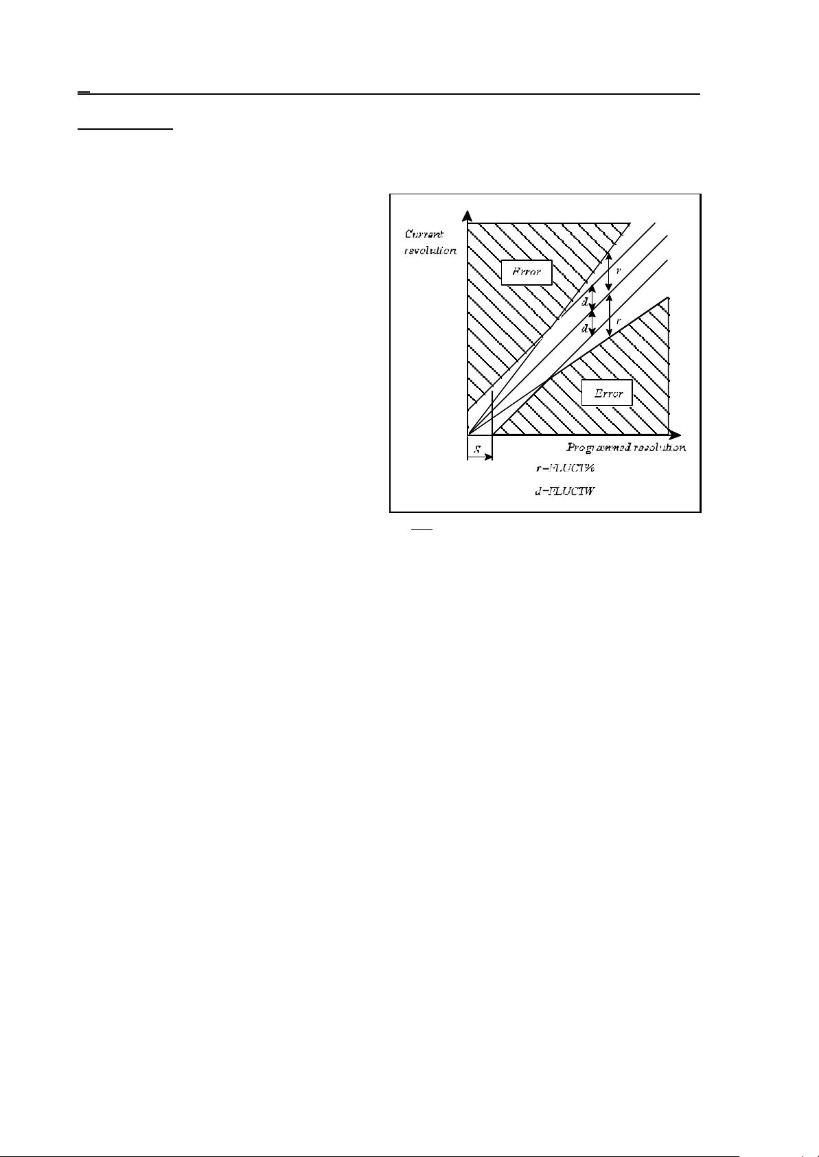
10 The Spindle Function
Detecting Error
In the course of detection the control sends error message in case the deviation between current and
specified spindle speed exceeds
- the tolerance limit specified by value "r" in
percent of the command value and
- also the absolute tolerance limit specified by
value "d"
When the current speed has exceeded both
tolerance limits, the NC sets flag I656 to PLC.
The speed range, in which the NC issues
alarm, can be seen on the 3rd figure. If the
specified spindle speed is under value "S"
apparent in the figure, the NC issues alarm,
provided the current speed is 0 revs/min for
more than 1 second.
– The spindle speed fluctuation detection is
effective only if the spindle is mounted
with encoder.
– The specified spindle speed, according to
Fig. 10.6-3
which the current spindle speed is
detected is calculated by taking the
override, the revolution range limits and the programmed maximum revolution (G92 S_) in
constant surface speed calculation (G96) into account.
– The spindle speed fluctuation detection is effective only in case of G26 and rotating spindle (state
M3 or M4).
– Command G26 must be programmed in single block.
68
Page 69

11 Tool Function
11 Tool Function
11.1 Tool Select Command (Code T)
With a number of max. four digits written at address T, the NC will give a code to the PLC.
When a movement command and a tool number (T) are programmed in a given block, function T
will be issued during or after the motion command. The machine tool builder will define the way of
execution.
11.2 Program Format for Tool Number Programming
There are basically two different ways of making reference to a tool change in the part program.
They depend on the configuration of the machine-tool. The particular technique of calling the tool
(applicable in the part program) is defined by the builder of the machine-tool.
Case A
A tool change can be accomplished on the machine manually or by means of a turret type tool
changer. Now, with reference made to code T:
– in the case of manual tool change, the number of tool to be used appears on the display; it has to
be clamped in the spindle manually. Afterwards, the machining will be resumed upon a start;
– in the case of a turret type tool changer, the new tool will be put to position of use automatically
under the action of code T.
Thus a reference to the tool number will evoke an immediate change in the block which T has been
specified in.
Case B
A tool change needs some preparations on the machine. Its steps:
– The tool to be employed has to be found in the magazine. Now reference to address T in the part
program will bring the appropriate tool in change position. This operation is carried out in
the background, simultaneously with the machining.
– The slides (or only one of them) have to be sent to the change positions.
– The tool change is carried out by function M06 in the program. The control will wait for the
execution of the tool change until tool T (under preparation) is brought to change position.
As a result, the new tool will be placed in the spindle. Henceforth cutting may be resumed.
– The old tool is replaced in the tool magazine. This activity is performed in the background,
simultaneously with cutting.
– The search is commenced for the new tool in the magazine.
69
Page 70

11 Tool Function
This procedure is described in the part program as follows.
Part Program Explanation
.................
....Tnnnn........ search for tool Tnnnn
................. the part program is running, tool search is being performed in the
background
...M06 Tmmmm.... tool Tnnnn is placed in the spindle,
................. the previous tool is replaced in the tool magazine
................. the search is commenced for tool Tmmmm, with cutting performed in
the meantime
...M06 Tpppp..... tool Tmmmm is placed in the spindle
................. tool Tnnnn is replaced in the tool magazine, search for tool Tpppp
begins
................. meanwhile machining is being performed
70
Page 71

12 Miscellaneous and Auxiliary Functions
12 Miscellaneous and Auxiliary Functions
12.1 Miscellaneous Functions (Codes M)
With a numerical value of max. 3 digits specified behind address M, the NC will transfer the code to
the PLC.
When a movement command and a miscellaneous function (M) are programmed in a given block,
function M will be issued during or after the motion command. The machine tool builder will define
the way of execution.
Codes M’s include standard functions, that can be used for special selected functions only. They:
The rest of M values can be used without restrictions.
When indexing is triggered by M, the M codes of spindle indexing are selected on the basis of a
parameter.
The control system enables several M codes of different groups to be written in a given block. In
this case, however, codes M’s have a fixed sequence of execution. The groups and the sequence of
execution:
The number of M functions that can be programmed in a given block is 5. Only one M of each
group can be programmed in a block. Conflicting programming will produce error message 3032
CONFLICTING M CODES.
The exact functioning of each M code is defined by the builder of the particular machine-tool to
meet its specific requirements. The only exceptions are the program control codes.
M00, M01, M02, M30, M96, M97, M98, M99: program control codes
M03, M04, M05, M19: Spindle rotation codes
M06: tool change code
M07, M08, M09: coolant management codes
M11, ..., M18: spindle-range changes codes
group 1 M06 (tool exchange)
group 2 M11, ..., M18 (spindle gear range change)
group 3 M03, M04, M05, M19 (spindle management)
group 4 M07, M08, M09 (coolant management)
group 5 Mnnn (any other function M)
group 6 codes M of spindle indexing
group 7 M00, M01, M02, M30, M96, M97, M98, M99 (program control codes)
The program control M codes are:
M00= programmed stop
The stop condition will be generated at the end of the block, in which M00 has been specified. All
modal functions remain unchanged. It can be restarted by START.
M01= conditional stop
Its effect is identical with that of code M00. It will be executed when the CONDITIONAL STOP
key is activated. Unless the appropriate key is set up, it is ineffective.
M02, M30= end of program
It means the end of the main program. All operations are stopped, and the control is "reset". The
machine will be reset by the PLC program. Unless the parameter PRTCNTM differ from it, each of
executed M02 or M03 command increase the counters of workpiece.
71
Page 72

12 Miscellaneous and Auxiliary Functions
M98= call of a subprogram (subroutine)
It will call a subprogram (subroutine).
M99= end of subprogram (subroutine)
It will cause the execution to return to the position of call.
12.2 Auxiliary Function (Codes A, B, C)
Max. three digits can be specified at each of addresses A, B, C provided one (or all) of those
addresses is (are) selected as auxiliary function(s) in parameters. The value specified for the auxiliary
function will be transferred to the PLC.
When a movement command and an auxiliary function are programmed in a given block, function A,
B, C will be issued during or after the motion command. The machine tool builder will define the
way of execution.
For example, an indexing table can be indexed at address B.
12.3 Sequence of Execution of Various Functions
The various functions written in a given block will be executed by the control in the following
sequence:
1. Tool change: M06
2. Tool call: T
3. Spindle range selection: M11, ..., M18
4. Spindle speed: S
5. Spindle management: M03, M04, M05, M19
6. Coolant: M07, M08, M09
7. Other function M: Mnnn
8. Spindle indexing: with function M
9. Function A: A
10. Function B: B
11. Function C: C
12. Program control codes: M00, M01, M02, M30, M96, M97, M98, M99
If the above sequence of executions is not desirable, the block has to be broken up into several
ones, with the functions written in the desired sequence in each block.
72
Page 73

13 Part Program Configuration
13 Part Program Configuration
The structure of the part program has been described already in the introduction presenting the
codes and formats of the programs in the memory. This Section will discuss the procedures of
organizing the part programs.
13.1 Sequence Number (Address N)
The blocks of the program can be specified with serial or sequence numbers. The numbering can be
accomplished at address N. The blocks can be numbered with max. 5 digits at address N. The use
of address N is not mandatory. Some blocks can be numbered, others not. The block numbers need
not follow each other in a consecutive order.
13.2 Conditional Block Skip
A conditional block skip can be programmed at the slash address /. The value of the slash address
may be 1 to 9. Digit 1 to 9 represents serial number of switches .
Switch CONDITIONAL BLOCK No. 1 can be found on the operator’s panel of control.
The other switches may be provided optionally, their signals can be entered through the interface of
the control system.
If a conditional block skip /n is programmed at the beginning of a block,
– that block will be omitted from the execution when the nth switch is on,
– that block will be executed when the nth switch is off.
13.3 Main Program and Sub-program
Two different programs are differentiated - main program and subprogram. Repetitive activities may
be involved in machining a component part, that can be described with a particular program detail.
In order to avoid writing the repetitive program detail over and over again in the program, they can
be organized into a subprogram to be called from the part program. The structures of the main
program and the subprogram have been described in the Introduction.
The difference between them is that, whereas the machining is completed after execution of the main
program the control is awaiting another START, while after execution of the subprogram it will
return to the calling program, resuming the machining process at that point.
In terms of programming technique, the difference between the two programs lies in the way of
terminating the program. The end of the main program is specified with codes M02 or M30 (not
mandatory ones), whereas the sub-program must be terminated with code M99.
13.3.1 Calling the Sub-program
The series of instructions
M98 P....
will generate a subprogram call. As a result, the execution of the program will be resumed at the
subprogram, the number of which is defined at address P. The limit of address P are 1 to 9999.
After the execution of the sub-program machining will be continued in the main program with the
block following the subprogram call.
73
Page 74
13 Part Program Configuration
main program
O0010
......
......
M98 P0011 –––> O0011 calling sub-program
next block <––– M99 return to the calling
......
......
subprogram comment
execution of (main-)
program O0010
O0011
......
......
......
execution of sub-
program O0011
program
resumption of program
O0010
The series of instructions
M98 P.... L....
will call the subprogram (specified at address P) repeteatedly in succession specified at address L.
The limit of address L is 1 to 9999. Unless L is assigned a value, the sub-program will be called
once, i.e., the control will assume L=1.
Instruction M98 P11 L6 means that subprogram 011 has to be called six times repeatedly.
It is also possible to call a subprogram from another subprogram. The subprogram calls can be
"nested" to max. 4 levels.
main program
O0001 >O0011 >O0012 >O0013 >O0014
.... .... .... .... ....
....
M98P11
....<
.... .... .... .... ....
M02 M99 M99 M99 M99
subprogram subprogram subprogram subprogram
.... .... .... ....
M98P12 M98P13 M98P14 ....
....< ....< ....< ....
L Notes:
– An error message 3069 LEVEL EXCESS is returned when the number of subprogram calls
"nested" exceeds 4.
– An error message 3071 MISSING OR FAULTY P is returned when the value of address P
exceeds 9999 or is not specified.
– An error message 3072 DEFINITION ERROR L is returned when the value of L is incorrect.
– An error message 3073 NOT EXISTING PROGRAM is returned when a program specified with
an identifier at address P is not available in the memory.
13.3.2 Return from a Sub-program
The use of instruction
M99
in a sub-program means the end of that sub-program, and the program execution returns to the
block following the call in the calling program.
74
Page 75

13 Part Program Configuration
main program
O0010
......
......
......
N101 M98 P0011
N102 ......
......
......
–––>
<–––
subprogram comment
execution of program
O0010
O0011 calling sub-program
O0011
......
......
......
M99 return to the next
execution of sub-
program O0011
block of the calling
program
resumption of program
O0010
The use of instruction
M99 P...
in a sub-program means the end of that sub-program, and the program execution returns to the
block of calling program specified at address P. In this case the limit values of P are to 99999.
main program
subprogram comment
O0010
......
......
......
N101 M98 P0011 –––> O0011 calling sub-program
......
......
......
N250 ...... <––– M99 P250 return to the N250
......
......
execution of program
O0010
O0011
execution of
subprogram O0011
block of the calling
program resumption of
O0010
Instruction
M99 (P.....) L....
will rewrite the cycle counter of the calling program. With 0 written for L, the sub-program will be
called only once. If, e.g., subprogram O0011 is called with instruction M98 P11 L20, and a return
is made with instruction M99 L5, subprogram O0011 will be called 6 times. (The limit values of L
are 1 to 9999.)
L Note:
– An error message 3070 NOT EXISTING BLOCK NO. P is displayed when the return block
number (P) is not found in the calling program.
75
Page 76

13 Part Program Configuration
13.3.3 Jump within the Main Program
The use of instruction
M99
in the main program will produce an unconditional jump to the first block of the main program, and
the execution of the program will be resumed there. The use of this instruction results in an endless
cycle:
O0123
N1...
...
.....
.....
M99
<
The use of instruction
M99 P.....
will produce an unconditional jump to the block specified at address P of the main program, and the
execution of the program will be resumed there. The use of this instruction results in an endless cycle:
O0011 O0011
....
....
N128....< ....
.... ....
.... N225 <
M99 P128
....
M99 P225
....
The possibility of endless cycles can be avoided by specifying the block containing instruction M99
in the form /1 M99. Now the jump will be omitted or not, depending on the setting of the conditional
block skip switch.
76
Page 77
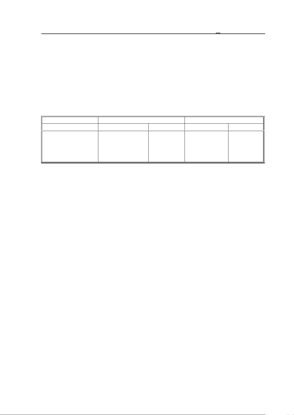
14 The Tool Compensation
14 The Tool Compensation
14.1 Referring to Tool Compensation Values (H and D)
Reference can be made to
tool length compensation at address H,
tool radius compensation at address D.
The number behind the address (the tool compensation number) indicates the particular
compensation value to be applied. The limit values of addresses H and D are 0 to 999.
The Table below shows the division of the compensation memory.
Code H Code D
compensation number geometry wear geometry wear
01
02
.
.
.
-350.200
830.500
0.130
-0.102
-32.120
52.328
.
.
.
0.012
-0.008
.
.
.
Compensation number 00 is not included in the above Table, the compensation values pertaining to
it are always zero.
Geometry value - the length/radius of the tool. It is a signed number.
Wear - the wear occurring in the course of machining. It is a signed number.
Whenever a reference is made to a compensation at address H or D in the program, the control will
always take the sum of the geometry value and the wear into account for compensation. If, e.g.,
reference is made to H2 in the program, the length compensation will be, on the basis of the above
Table, 830.500+(–0.102)=830.398.
Address H and D are modal ones, i.e., the control will take into account a given compensation value
until another command D or H is given. In other words, once the compensation value has been read
with command D or H, the read-out value will be unaffected by a change in the chart of
compensation values (e.g., by programming G10).
The compensation values will be preserved in the memory after a power-off.
The compensation memory can be saved in the memory as a part program.
77
Page 78
14 The Tool Compensation
Limit values of geometry and wear:
input units output units
mm mm
inch mm
inch inch
mm inch
increment
system
IS-A ±0.01 ÷99999.99 ±0.01÷163.80
IS-C ±0.0001÷999.9999 ±0.0001÷1.6380
IS-A ±0.001÷9999.999 ±0.001÷6.448
IS-C ±0.00001÷99.99999 ±0.00001÷0.06448
IS-A ±0.001÷9999.999 ±0.001÷16.380
IS-C ±0.00001÷99.99999 ±0.00001÷0.16380
IS-A ±0.01÷99999.99 ±0.01÷416.05
IS-C ±0.0001÷999.9999 ±0.0001÷4.1605
geometry value wear value
unit of
measure
mmIS-B ±0.001÷9999.999 ±0.001÷16.380
inchIS-B ±0.0001÷999.9999 ±0.0001÷0.6448
inchIS-B ±0.0001÷999.9999 ±0.0001÷1.6380
mmIS-B ±0.001÷9999.999 ±0.001÷41.605
The tool compensations can be selected and/or modified from the operator's panel on OFFSET
screen and from the program with the use of instruction G10. If the current compensation is modified
with command G10, reference has to be made again to the current compensation register D or H, or
else the modified value will be disregarded.
The limit values of address H or D for the given control system, i.e., the numbers of length and
radius compensations to be specified in that control system, are determined by the memory
configuration of the control. In the case of a minimum memory configuration, the number of
compensations is 99, i.e., the limit values of addresses H and D are 0 to 99.
14.2 Modification of Tool Compensation Values from the Program (G10)
Instruction
G10 R L P
can be used for modifying the tool compensations from the program. G10 is a one-shot instruction.
The addresses and their values have the following meanings.
The compensation value is specified at address R. At G90 (absolute data specification command),
the value written at address R will be transferred to the appropriate compensation register. At G91
(incremental data specification command) or when operator I is applied, the data written at address
R will be added to the content of the appropriate compensation register.
The compensation value to be modified is specified at address L:
L=10 applies to the geometry value of the length compensation (code H),
L=11 applies to the wear of the length compensation (code H),
L=12 applies to the geometry value of the radius compensation (code H)
L=13 applies to the wear of the radius compensation (code H),
The No. of compensation value to be modified is specified at address P.
L Note: For a programmed modification of the tool radius compensation, the value specified at
address R must be interpreted as a radius in each case regardless of the state of parameter
TOOLRAD . The control will return error message 3001 VALUE EXCESS X,Y,...F
whenever the specified values exceed the limits contained in the above Table.
78
Page 79

14 The Tool Compensation
14.3 Tool Length Compensation (G43, G44, G49)
Instruction
G43 q H or
G44 q H
will set up the tool length compensation mode.
Address q means axis q to which the tool length compensation is applied (q= X, Y, Z, U, V, W, A,
B, C).
Address H means the compensation cell, from which the tool length compensation value is taken.
Irrespective of q being an absolute or an incremental data, instruction G43 will add the
compensation value (specified at address H) to the end point coordinate obtained in the course of
execution:
G43: + compensation
Irrespective of q being an absolute or an incremental data, instruction G44 will subtract the
compensation (specified at address H) from the end point coordinate obtained in the course of
execution:
G44: – compensation
Since incremental displacement Z0 has been programmed, each of instructions G43 G91 Z0 H1 and
G44 G91 Z0 H1 will produce displacement just equal to the length of the tool. At G43, the
displacement will be positive or negative, depending on the compensation value at H1 being positive
or negative, respectively. The case is just the opposite for G44. After the command has been
executed, the position displayed at coordinate Z will be the same as the one beforehand, because
the position of the tool's tip will be displayed after the length compensation is set up.
Tool compensations may be defined on several axes at a time. E.g.
G43 Z250 H15
G43 W310 H16
When several axes are selected in a block, the tool length compensation will be taken into account
for each axis selected:
G44 X120 Z250 H27
When the composition value is altered by calling a new H address, the previous one will be deleted,
and the new value will be effective:
H1=10, H2=20
G90 G00
G43 Z100 H1..........moving to Z=110
G43 Z100 H2..........moving to Z=120
The effects of G43 and G44 are modal until another command is received from that group.
Command
G49 or
H00
will cancel the tool length compensation in each axis - with motion or with transformation, if a
movement has been programmed in the block or not, respectively.
The difference between the two commands is that H00 will delete the compensation only, leaving
state G43 or G44 unaffected. If a reference is made afterwards to an address H other than zero, the
new tool length compensation will be set up as the function of state G43 or G44.
79
Page 80
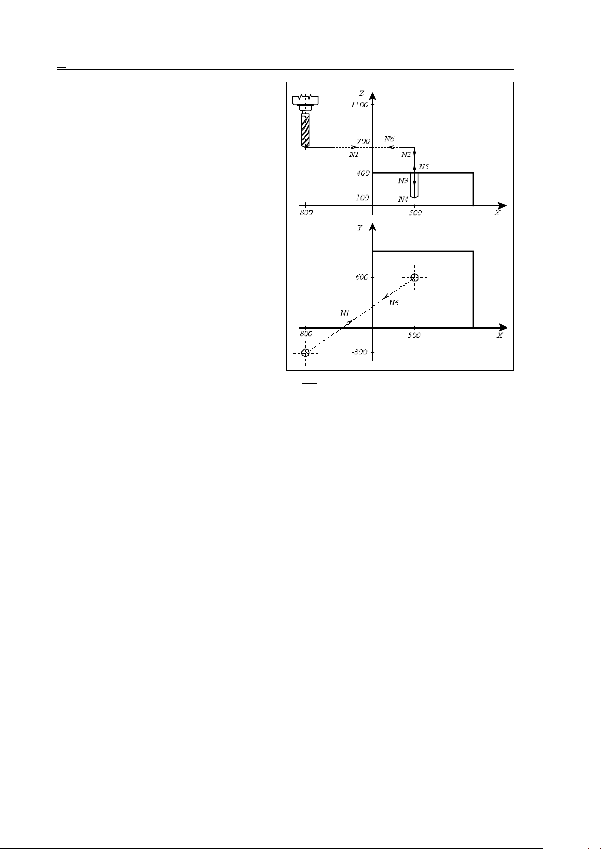
14 The Tool Compensation
If, however, instruction G49 is used, any
reference to address H will be ineffective until
G43 or G44 is programmed.
At power-on, the value defined in parameter
group CODES decides which code is effective
(G43, G44, G49).
The example below presents a simple drilling
operation with tool length compensation taken
into account:
length of drilling tool, H1=400
Fig. 14.3-1
N1 G90 G0 X500 Y600 (positioning in plane X, Y)
N2 G43 Z410 H1 (moving to Z410 with H1 length compensation)
N3 G1 Z100 F180 (drilling as far as Z100 with F180 feed)
N4 G4 P2 (dwell for 2 seconds)
N5 G0 Z1100 H0 (removing the tool and canceling the length
compensation; the tool's tip is in the X700 point)
N6 X-800 Y-300 (returning with rapid traverse in plane X, Y)
14.4 Tool Offset (G45...G48)
G45 increases the movement amount with the offset value
G46 decreases the movement amount with the offset value
G47 increases the movement amount by twice with the offset value
G48 decreases the movement amount by twice with the offset value
Any one of commands G45...G48 will be effective with the compensation selected with the D code
until another value is called in conjunction with a command G45...G48.
Being non-modal codes, they are effective only in the block in which they have been specified.
In the case of an absolute data specification, the amount of movement will be the difference between
the end point defined in the current block and the end point of the previous block. Any increase or
decrease refers to the direction of motion produced in this way.
80
Page 81
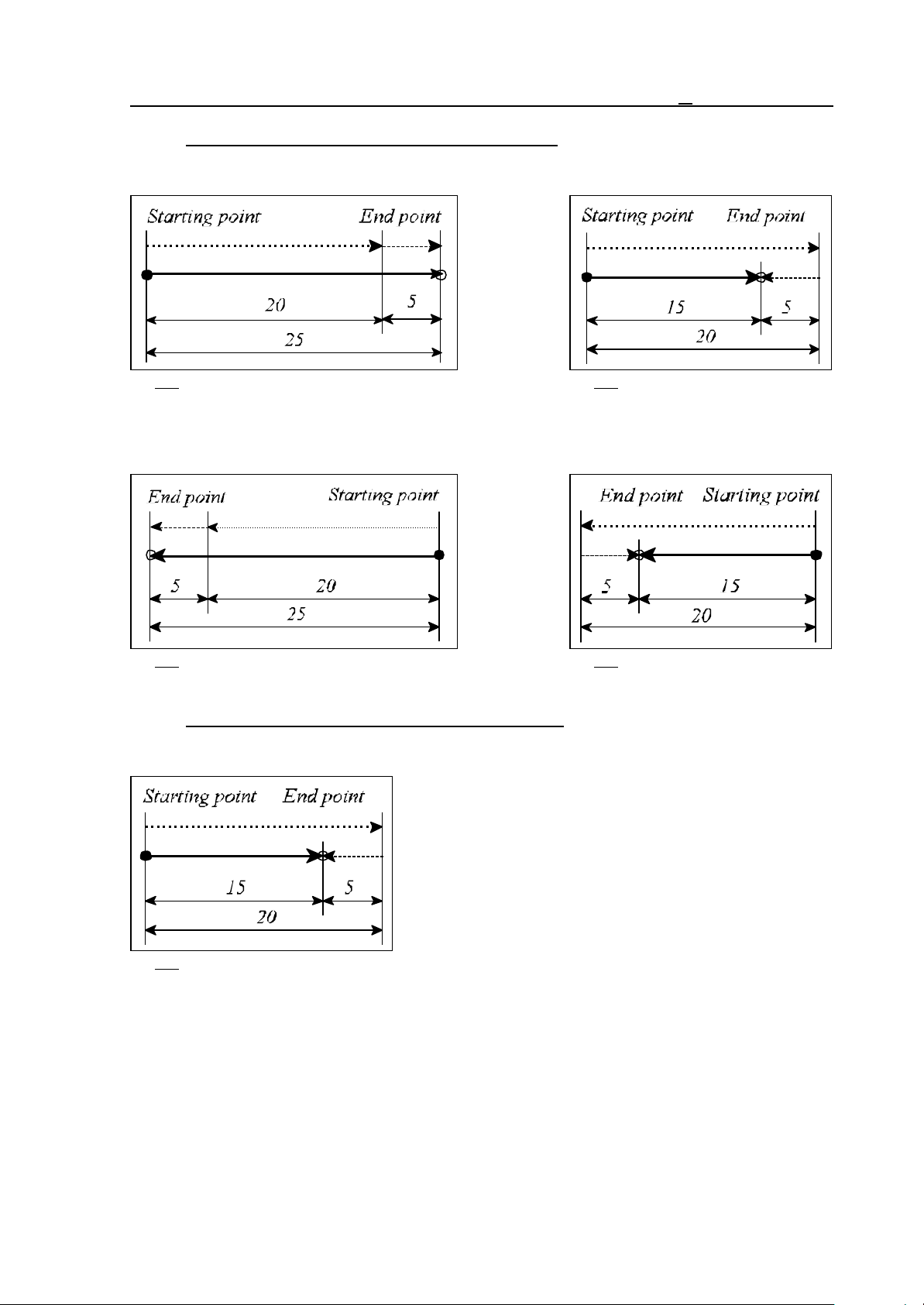
14 The Tool Compensation
With G45 programmed (increase by the offset value):
a. movement command: 20 b. movement command: 20
compensation: 5 compensation: -5
Fig. 14.4-1 Fig. 14.4-2
a. movement command: -20 b. movement command: -20
compensation: 5 compensation: -5
Fig. 14.4-3 Fig. 14.4-4
With G46 programmed (decrease by the offset value):
a. movement command: 20 cases b, c, d are similar to G45
compensation: 5
Fig. 14.4-5
81
Page 82
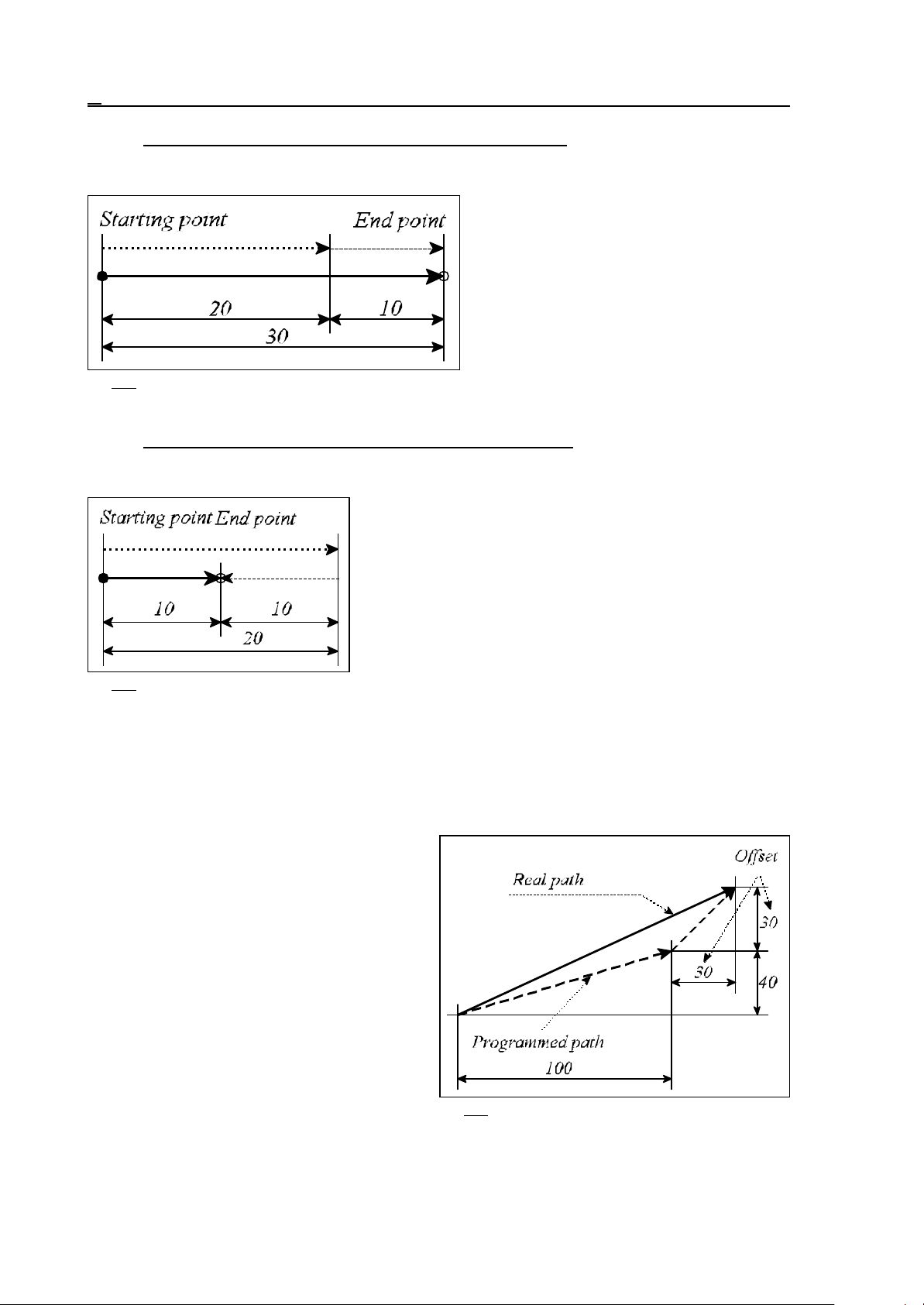
14 The Tool Compensation
With G47 programmed (double increase by the offset value):
a. movement command: 20 cases b, c, d are similar to G45
compensation: 5
Fig. 14.4-6
With G48 programmed (double decrease by the offset value):
a. movement command: 20 cases b, c, d are similar to G45
compensation: 5
Fig. 14.4-7
If, after command G45...G48, movement commands are issued for several axes in the block, the
resultant compensation will be effective in each programmed axis separately, with the value specified
at D (non-vectorially generated).
If, e.g., D1=30, command G91 G45 G1 X100 Y40 D1 will produce displacements of x=130,
y=70.
The resultant compensations cannot be deleted
with a common G command (e.g., G49 for
length compensation) or by programming D00,
only with a command G45...G48 of opposite
meaning.
In the use of G45...G48, only one D code may
be applied, or else the control will return the
error message 3008 ERRONEOUS
G45...G48.
If an incremental 0 displacement is programmed
together with one of commands G45...G48, a
sign preceding the 0 will also be interpreted by
Fig. 14.4-8
the control as follows:
if D1=12
82
Page 83
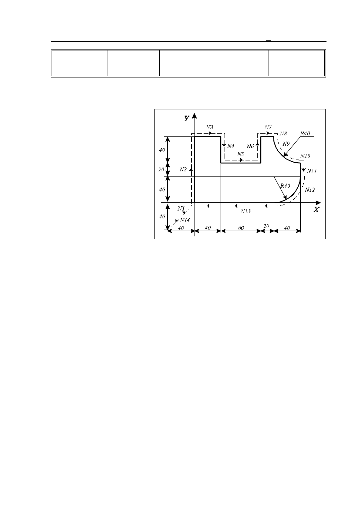
14 The Tool Compensation
NC command G45 XI0 D1 G46 XI0 D1 G45 XI-0 D1 G46 XI-0 D1
displacement x=12 x=-12 x=-12 x=12
A tool radius compensation applied with one of codes G45...G48 is also applicable with ¼ and ¾
circles, provided the centers of the circles are specified at address I, J or K.
An example: D1=10
N1 G91 G46 G0 X40 Y40 D1
N2 G47 G1 Y100 F180
N3 G47 X40
N4 Y-40
N5 G48 X60
N6 Y40
N7 G47 X20
N8 G45 Y–0
N9 G46 G3 X40 Y–40 I40
N10 G45 G1 X0
N11 G45 Y–20
N12 G45 G2 X–40 Y–40 I–40
N13 G45 G1 X–120
N14 G46 G0 X–40 Y–40
Fig. 14.4-9
83
Page 84
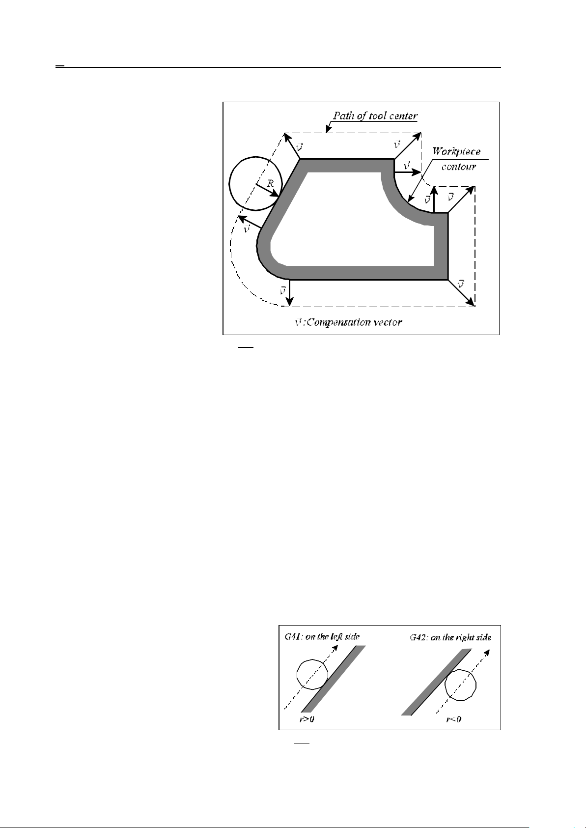
14 The Tool Compensation
14.5 Cutter Compensation (G38, G39, G40, G41, G42)
To be able to mill the contour of a
two-dimensional workpiece and to
specify the points of that formation
as per the drawing in the program
(regardless of the size of the tool
employed), the control must guide
the tool center parallel to the
programmed contour, spaced by a
tool radius from the latter. The
control will determine the distance
between the path of the tool center
and the programmed contour in
accordance with the compensation
value of the tool radius referred to
by compensation number D.
The compensation vector is a twodimensional vector computed over
Fig. 14.5-1
and over again by the control in each block, modifying the programmed displacements with the
compensation vectors effective at the beginning and end of each block. The length and direction of
each compensation vector obtained vary with the compensation value (called at address D) and the
geometry of the transition between the two blocks.
The compensation vectors are computed in the plane selected by instructions G17, G18, G19. This
is the plane of cutter compensation. Movements outside of this plane are not influenced by
compensation. If, e.g., plane X, Y is selected in state G17, the compensation vectors will be
computed in that plane. In this case any movement in Z direction it will be unaffected by the
compensation.
The compensation plane may not be changed while a tool radius compensation is being computed.
Any attempt to do so will result in an error message 3010 PLANE SELECT. IN G41, G42 by the
control.
If a compensation plane is to be defined with additional axes, they have to be defined as parallel
ones in parameters. If, e.g., U is assumed as a parallel axis and the tool radius compensation is to be
applied in plane Z, U, that plane can be selected by the specification of G18 U_Z_.
G40: Cutter compensation cancel
G41: Cutter compensation left
G42: Cutter compensation right
Command G41 or G42 will set up the
compensation computation. In state G41 or
G42 the programmed contours will be tracked
from left side or right side (seen from the travel
direction), respectively. The compensation
number of tool radii has to be specified at
address D. The specification of D00 is always
equivalent to calling zero radius value. The
Fig. 14.5-2
84
Page 85
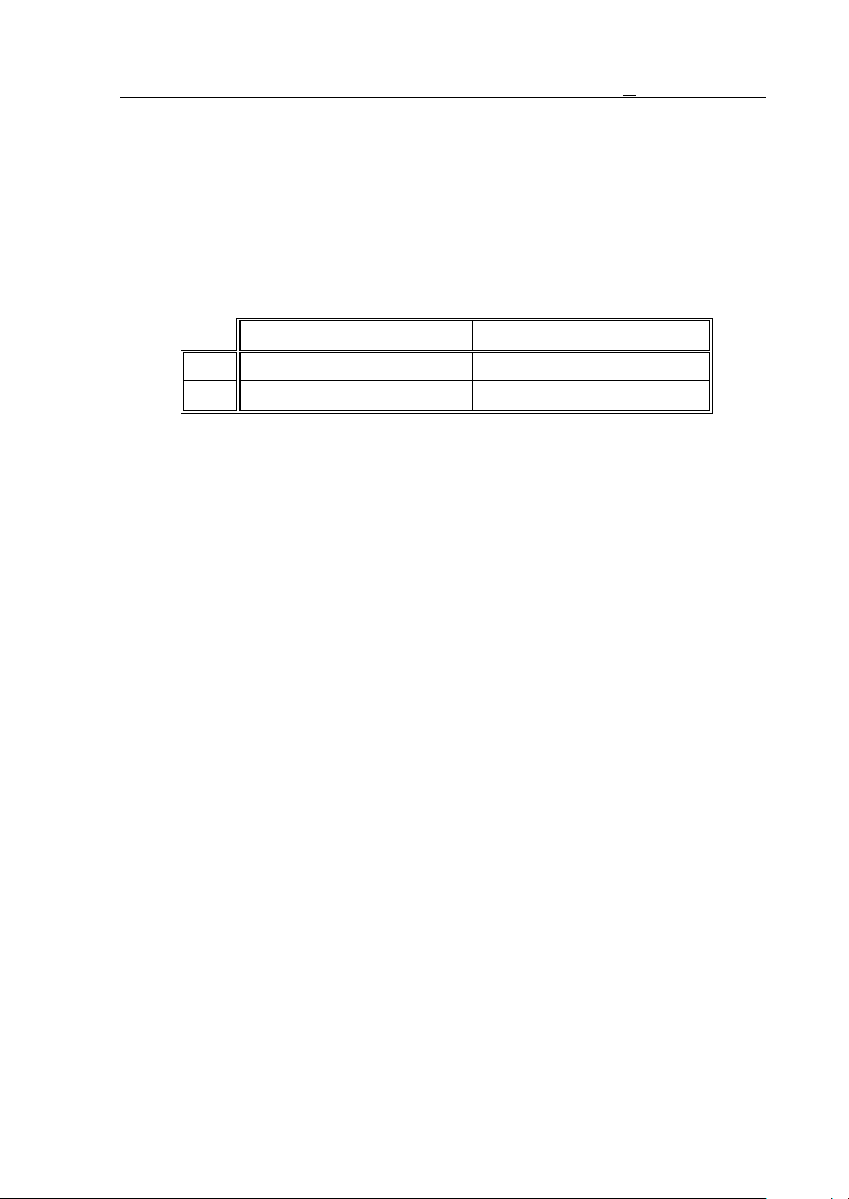
14 The Tool Compensation
compensation calculations are performed for interpolation movements G00, G01, G02, G03.
The above points refer to the specification of positive tool radius compensation, but its value may be
negative, too. It has a practical meaning if, e.g., a given subprogram is to be used for defining the
contours of a "female" part and of a "male" one being matched to the former. A possible way of
doing this is to mill the female part with G41 and the male part with G42. However, that changeover may be omitted from the program when the female part is machined with a positive radius
compensation, and the male part with a negative one. Now the path of the tool center is reversed
with respect to the programmed G41 or G42.
Radius compensation: positive Radius compensation: negative
G41 on the left side on the right side
G42 on the right side on the left side
L Note:
– For simplicity's sake, the subsequent descriptions and Figures will always refer to positive radius
compensations.
Command G40 or D00 will cancel the offset compensation. The difference between the two
commands is that D00 deletes only the compensation vector, leaving state G41 or G42 unchanged.
If a reference is made subsequently to an address D other than zero, the compensation vector will
be computed with the new tool radius as the function of state G41 or G42.
If, however, instruction G40 is used, any reference to address D will be ineffective until G41 or G42
has been programmed.
The procedure of setting up and canceling the radius compensation is detailed in the subsequent
sections.
Commands G40, G41, G42 are modal ones. The control will assume state G40 after power-on, at
the end of a program or in the event of resetting the program to its beginning, under such conditions
the radius compensation vectors will be deleted.
Radius compensation instructions will be carried out by the control in automatic mode only. It is
ineffective when programming a single block in manual mode. The reason of this is as follows. For
the control to be able to compute the compensation vector in the end point of a block
(interpolation), it must also read the next block containing the movement in the selected plane. The
compensation vector depends on the transition between the two interpolations. Accordingly, several
blocks (interpolations) have to be pre-processed for the calculation of a compensation vector.
85
Page 86
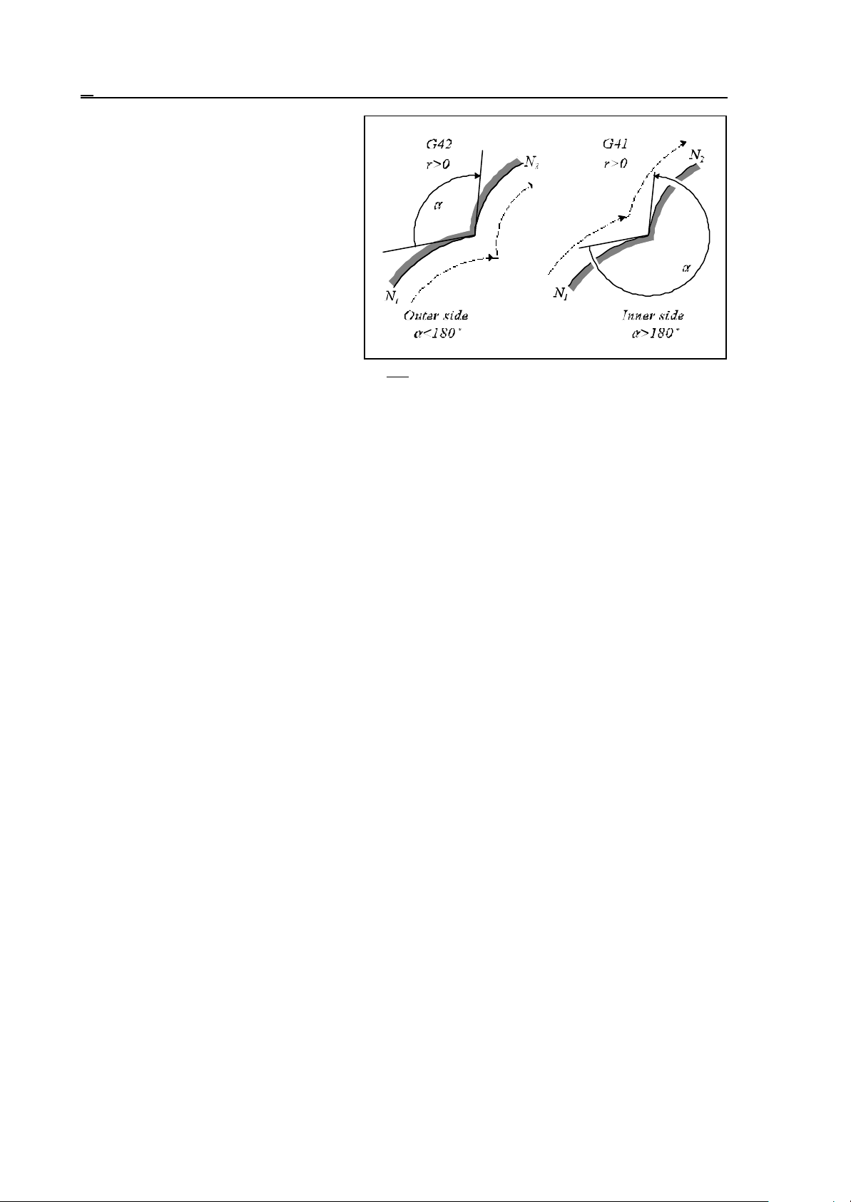
14 The Tool Compensation
An auxiliary data is to be introduced
before embarking on the discussion of the
details of the compensation computation.
It is """, the angle at the corner of two
consecutive blocks viewing from the
workpiece side. The direction of "
depends on whether the tool goes around
the corner from the left or right side.
The control will select the strategy of
going around in the intersection points as
the function of angle ". If ">180°, i.e.,
the tool is working inside, the control will
Fig. 14.5-3
compute a point of intersection between
the two interpolations. If "<180°, i.e., the tool is moving around the outside, it may add further
straight sections.
86
Page 87
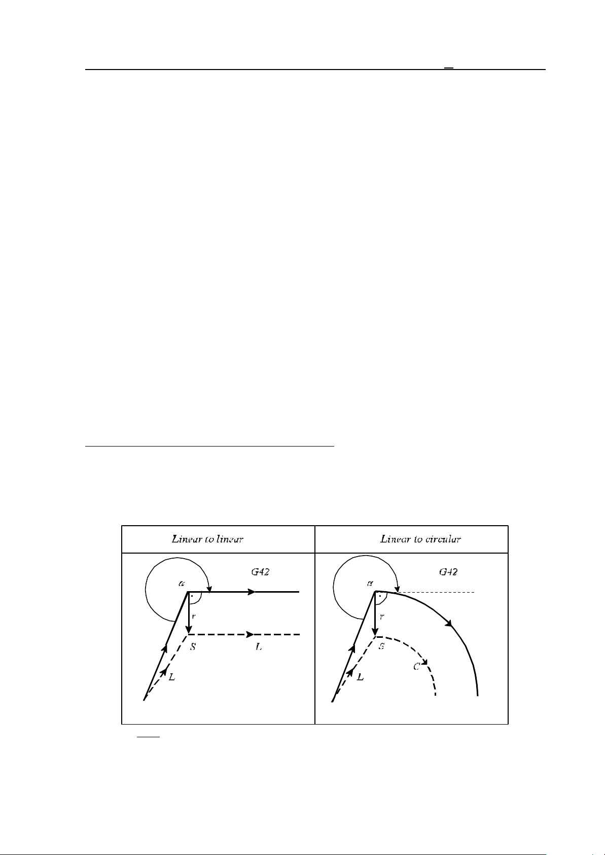
14 The Tool Compensation
14.5.1 Start up of Cutter Compensation
After power-on, end of program or resetting to the beginning of the program, the control will assume
state G40. The offset vector will be deleted, the path of the tool center will coincide with the
programmed path.
Under instruction G41 or G42 the control will exit from state G40 to enter in radius-compensation
computation mode. The value of compensation will be taken from the compensation cell (D
register). State G41 or G42 will only be assumed in a block containing a linear interpolation (G00 or
G01). The control will return error message 3043 G41, G42 IN G2, G3 to any attempt to set up
the compensation calculation in a circular interpolation (G02, G03). The control will only choose the
procedure of the start up of cutter compensation, if G41 or G42 was commanded after G40. In
other words, the control will not adopt the start up procedure when the compensation is deleted
with D00 and re-activated with Dnn (nn being a number other than 0).
The basic instances of starting compensation up depending on the angle of " at the corner of the two
consecutive blocks and the type of interpolations (linear-to-linear, linear-to-circular) as shown
below. The Figures refer to instance G42, positive radius compensation assumed.
L Note: The symbols in the Figures (below and afterwards) have the following meanings:
r: value of radius compensation,
L: straight line
C: circular arc,
S: single block stop point,
Dashed line: the path of tool center,
Continuos line: the programmed path.
Basic instances of starting up the cutter compensation:
(G40) (G40)
G42 G01 X_ Y_ D_ G42 G01 X_ Y_ D_
X_ Y_ G2 X_ Y_ R_
Going around an inside corner, 180°<"<360°
Fig. 14.5.1-1
87
Page 88
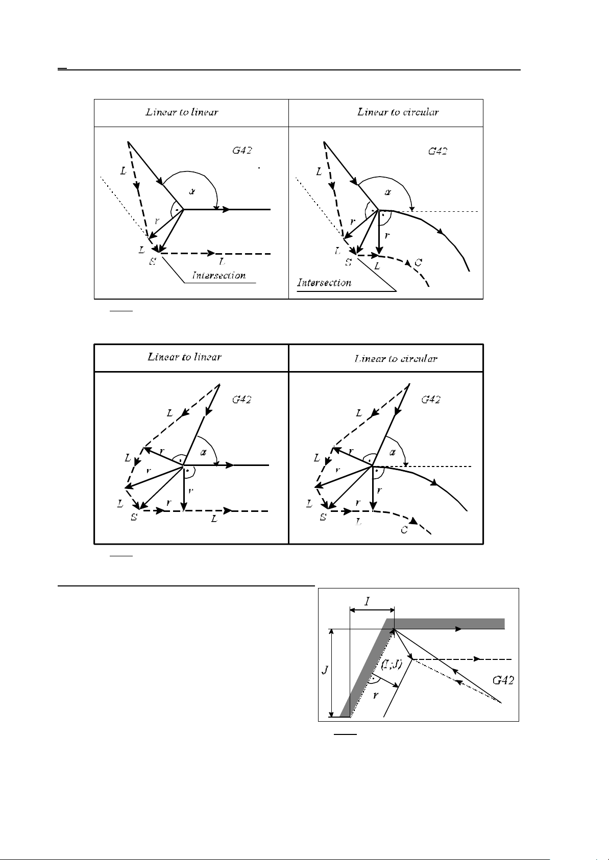
14 The Tool Compensation
Going around the outside of a corner at an obtuse angle, 90°#"#180°
Fig. 14.5.1-2
Going around the outside of a corner at an acute angle, 0°#"<90°
Fig. 14.5.1-3
Special instances of starting up the radius compensation:
If values are assigned to I, J, K in the compensationselecting block (G41 or G42) - but only to those in
the selected plane (e.g., to I, J in the case of G17) the control will move to the intersection point between
the next block and the straight line defined by I, J, K
with starting up radius compensation. The values of I,
J, K are always incremental ones, the vector defined
by them pointing to the end point of the interpolation,
in which it has been programmed. This facility is
useful, e.g., in moving to an inside corner.
88
Fig. 14.5.1-4
Page 89
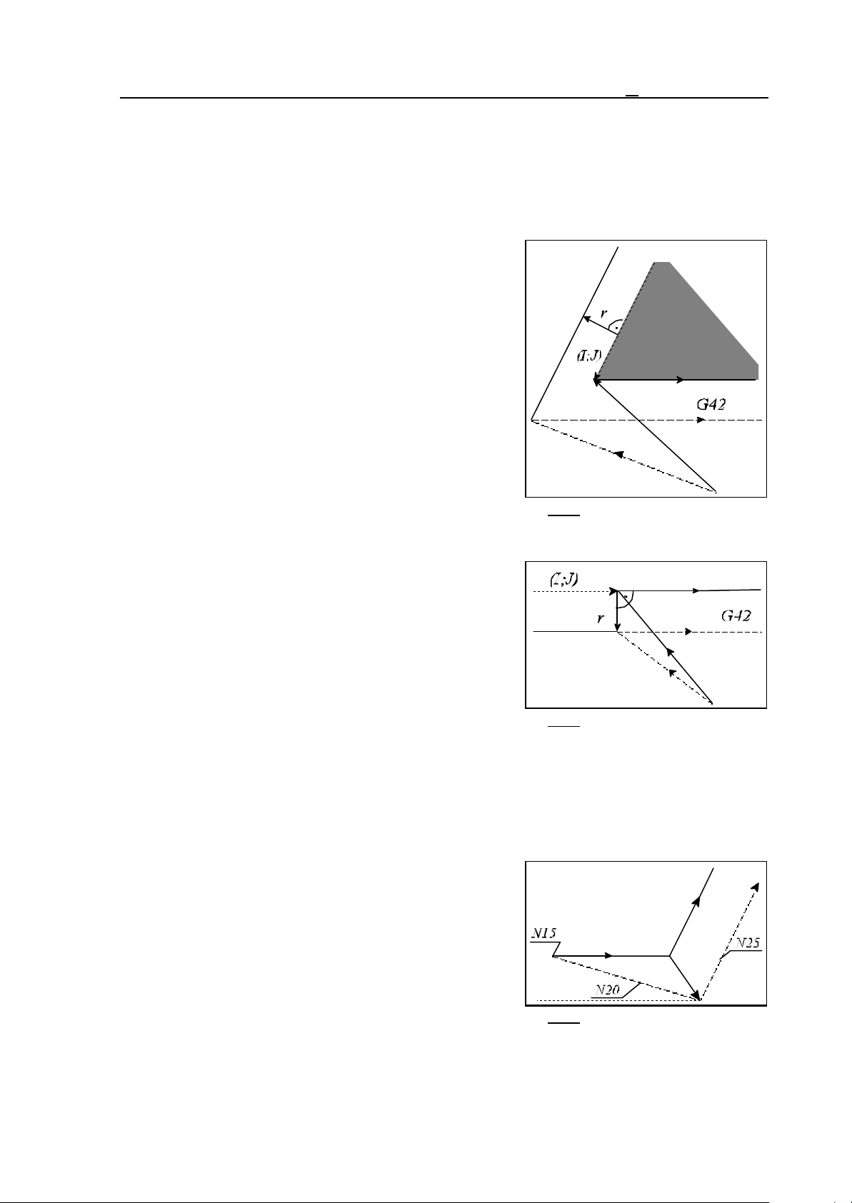
...
G91 G17 G40
...
N110 G42 G1 X-80 Y60 I50 J70 D1
N120 X100
...
In this case the control will always compute a point of
intersection regardless of whether an inside or an outside
corner is to be machined.
14 The Tool Compensation
Fig. 14.5.1-5
Unless a point of intersection is found, the control will move,
at right angles, to the start point of the next interpolation.
Fig. 14.5.1-6
When the compensation is set up by a special block in which no movement is programmed in the
selected plane, the compensation will be set up without any movement, the calculated compensation
vector’s length is 0. The compensation vector is computed at the end of the next motion block
according to the strategy corresponding to compensation computation in offset mode (see the next
chapter).
...
N10 G40 G17 G0 X0 Y0
N15 G42 D1
N20 G1 X80
N25 X110 Y60
...
Fig. 14.5.1-7
89
Page 90
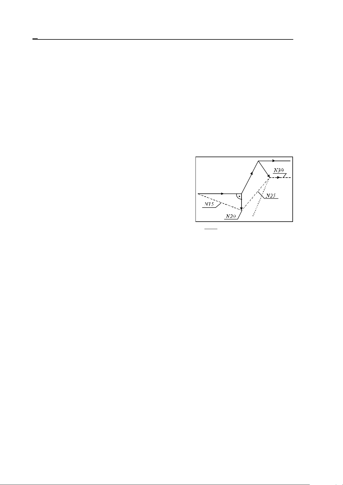
14 The Tool Compensation
If zero displacement is programmed (or such is produced) in the block containing the activation of
compensation (G41, G42), the control will not perform any movement but will carry on the
machining along the above-mentioned strategy.
...
N10 G40 G17 G0 X0 Y0
N15 G91 G42 D1 X0
N20 G1 X80
N25 X30 Y60
...
If a displacement of 0 is obtained in the selected plane in the block following the start-up of
compensation, the compensation vector will be set at right angles to the interpolation performing the
setting-up. The path of the tool in the next interpolation will be not parallel to the programmed
contour:
...
N10 G40 G17 G0 X0 Y0
N15 G91 G42 D1 X80
N20 G1 X0
N25 X30 Y60
N30 X60
...
Fig. 14.5.1-8
90
Page 91
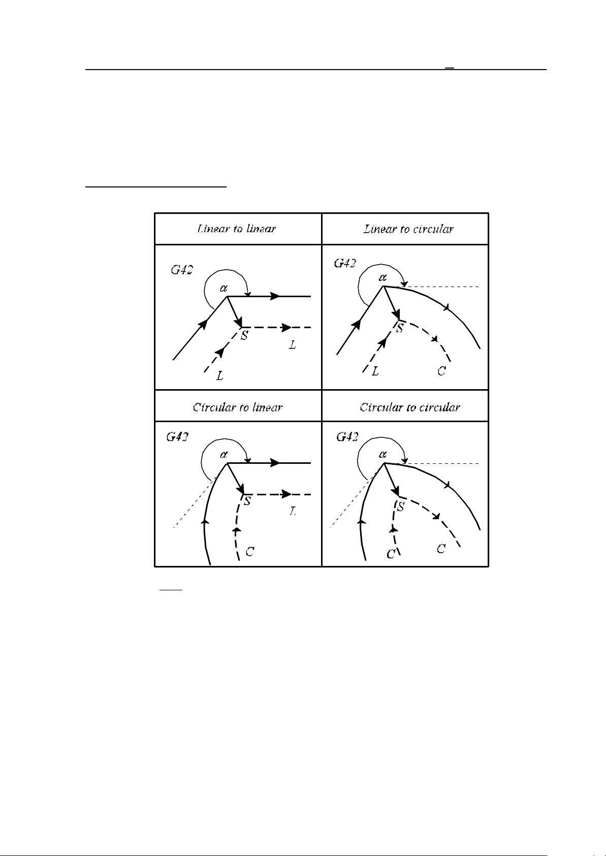
14 The Tool Compensation
14.5.2 Rules of Cutter Compensation in Offset Mode
In offset mode the compensation vectors will be calculated continuously between interpolation
blocks G00, G01, G02, G03 (see the basic instances) until more than one block will be inserted,
that do not contain displacements in the selected plane. This category includes a block containing
dwell or functions.
Basic instances of offset mode:
Computation of intersection point for inside corners, 180°<"<360°
Fig. 14.5.2-1
91
Page 92
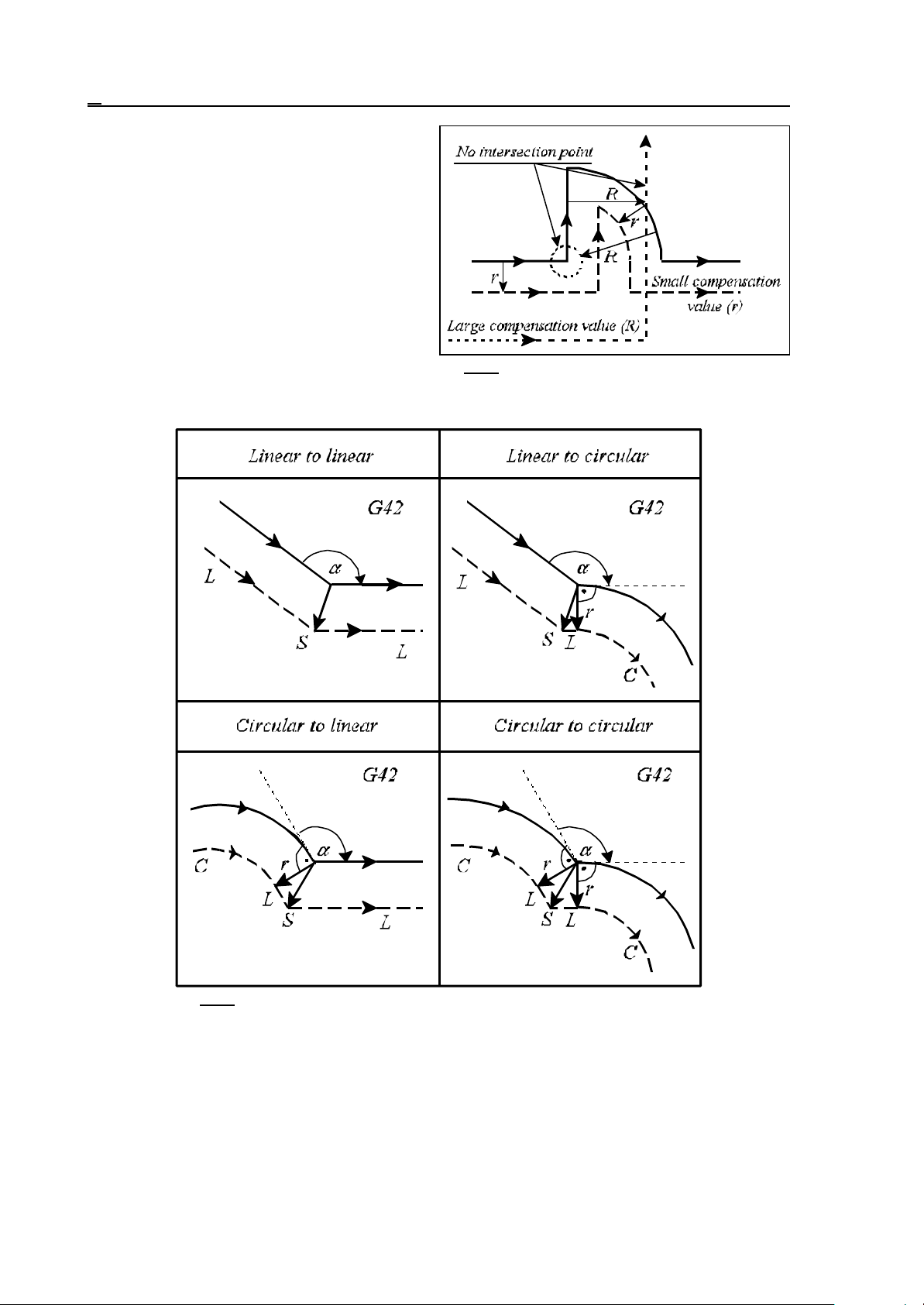
14 The Tool Compensation
It may occur that no intersection point is
obtained with some tool-radius values. In this
case the control comes to a halt during
execution of the previous interpolation and
returns error message 3046 NO INTER-
SECTION G41, G42.
Going around the outside of a corner at an obtuse angle, 90°#"#180°
Fig. 14.5.2-2
92
Fig. 14.5.2-3
Page 93
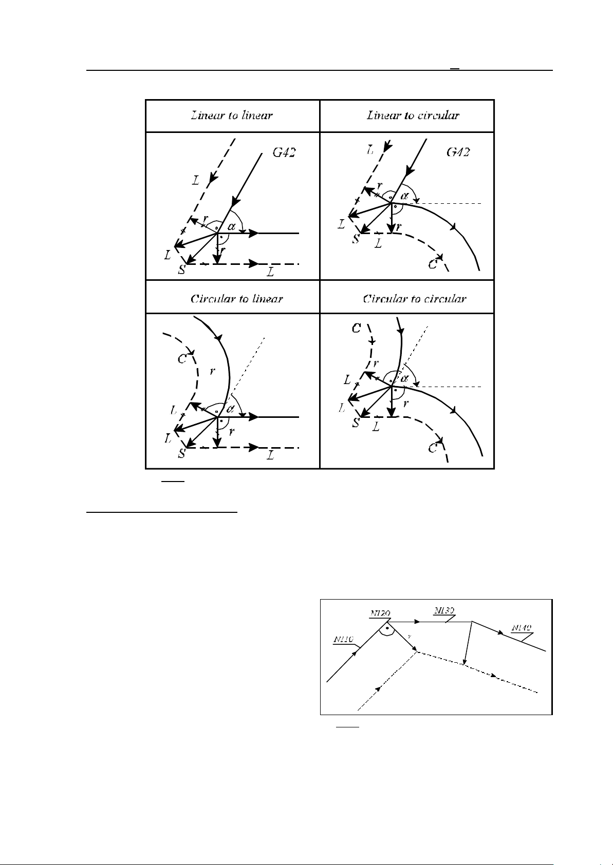
14 The Tool Compensation
Going around the outside of a corner at an acute angle, 0°#"<90°
Fig. 14.5.2-4
Special instances of offset mode:
If zero displacement is programmed (or such is obtained) in the selected plane in a block in offset
mode, a perpendicular vector will be positioned to the end point of the previous interpolation, the
length of the vector will be equal to the radius compensation. Instances of this kind should be
handled with caution because of the hazards of inadvertent undercutting or distortions (in the case of
a circle).
For example:
...G91 G17 G42...
N110 G1 X40 Y50
N120 X0
N130 X90
N140 X50 Y-20
...
Fig. 14.5.2-5
93
Page 94
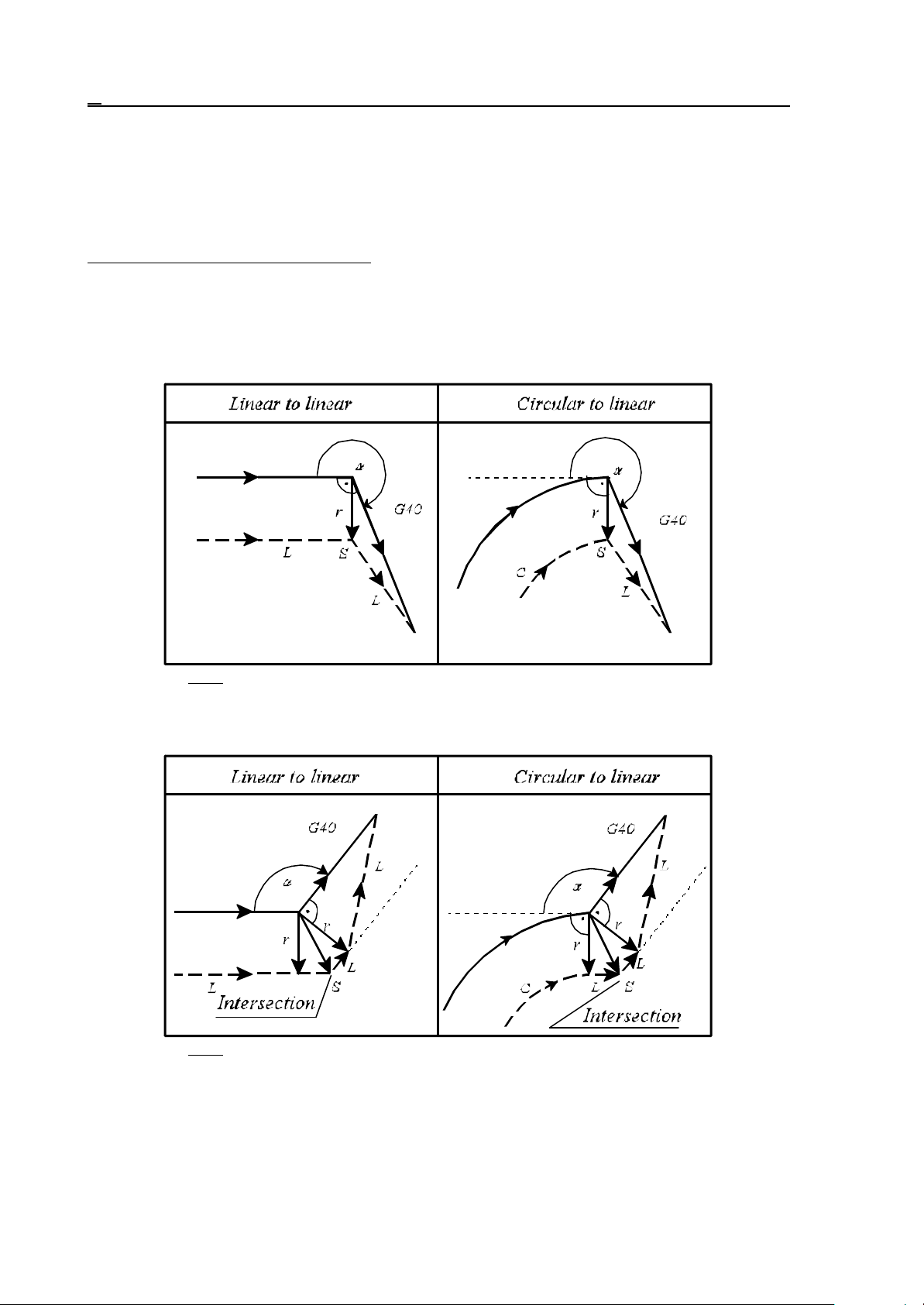
14 The Tool Compensation
14.5.3 Canceling of Offset Mode
Command G40 will cancel the computation of tool radius compensation. Such a command can be
issued with linear interpolation only. The control will return error message 3042 G40 IN G2, G3 to
any attempt to program G40 in a circular interpolation.
Basic instances of canceling offset mode:
(G42)
G01 X_ Y_
G40 X_ Y_
Fig. 14.5.3-1
(G42)
G02 X_ Y_ R_
G40 G1 X_ Y_
Going around an inside corner, 180°<"<360°
Going around the outside of a corner at an obtuse angle, 90°#"#180°
Fig. 14.5.3-2
94
Page 95
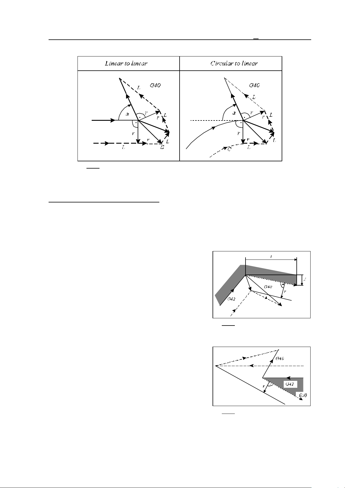
Going around the outside of a corner at an acute angle, 0°#"<90°
Fig. 14.5.3-3
Special instances of canceling offset mode:
14 The Tool Compensation
If values are assigned to I, J, K in the compensation cancel block (G40) - but only to those in the
selected plane (e.g., to I, J in the case of G17) - the control will move to the intersection point
between the previous interpolation and the straight line defined by I, J, K. The values of I, J, K are
always incremental, the vector defined by them points away from the end point of the previous
interpolation.
This facility is useful, e.g., for moving from an inside corner.
...
...G91 G17 G42...
N100 G1 X50 Y60
N110 G40 X70 Y-60 I100 J-20
...
Fig. 14.5.3-4
In this case the control will always compute a point of
intersection regardless of whether an inside or an outside
corner is to be machined.
Fig. 14.5.3-5
95
Page 96
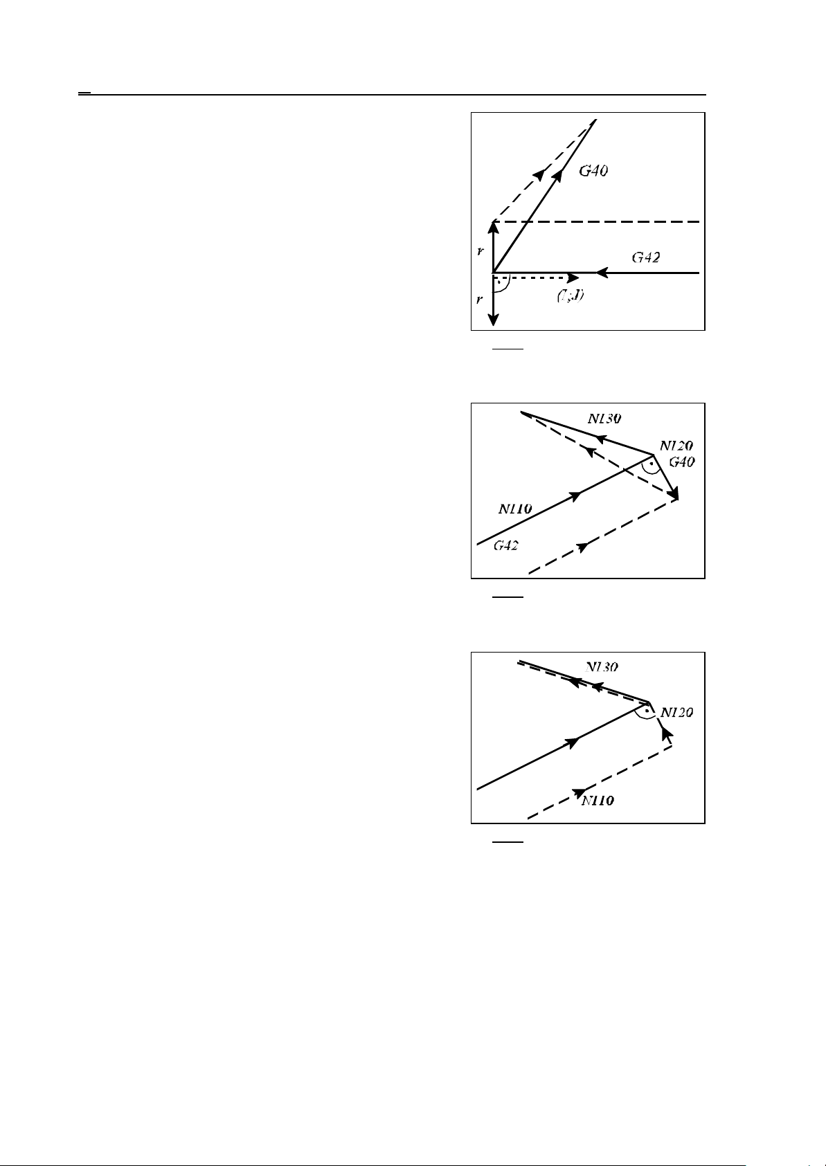
14 The Tool Compensation
Unless a point of intersection is found, the control will move,
at a right angle, to the end point of the previous interpolation.
If the compensation is canceled in a block in which no
movement is programmed in the selected plane, an offset
vector perpendicular to the end point of the previous
interpolation will be set and the compensation vector will be
deleted by the end of the next movement block.
...G42 G17 G91...
N110 G1 X80 Y40
N120 G40
N130 X-70 Y20
...
Fig. 14.5.3-6
Fig. 14.5.3-7
If zero displacement has been programmed (or such is
obtained) in the block (G40) in which the compensation is
canceled, an offset vector perpendicular to the end point of
the previous interpolation will be calculated, and the control
will cover that instance in block G40. For example:
...G42 G17 G91...
N110 G1 X80 Y40
N120 G40 X0
N130 X-70 Y20
...
Fig. 14.5.3-8
96
Page 97
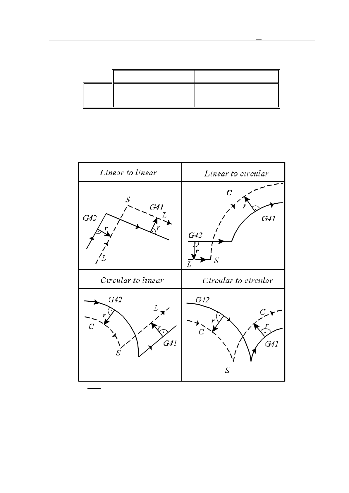
14 The Tool Compensation
14.5.4 Change of Offset Direction While in the Offset Mode
The direction of tool-radius compensation computation is given in the Table below.
Radius compensation: positive Radius compensation: negative
G41 left right
G42 right left
The direction of offset mode can be reversed even during the computation of tool radius
compensation. This can be accomplished by programming G41 or G42, or by calling a tool radius
compensation of an opposite sign at address D. When the direction of offset mode is reversed, the
control will not check it for being "outside", it will always calculate a point of intersection in first
steps. The Figures below assume positive tool radii and change-overs from G42 to G41.
Fig. 14.5.4-1
97
Page 98
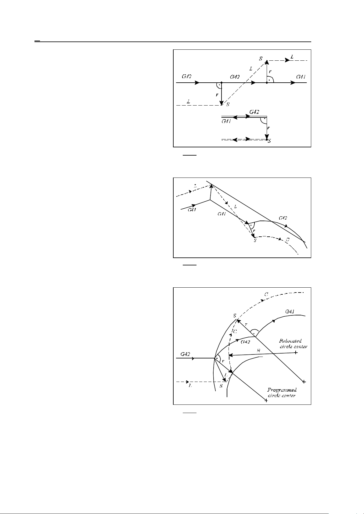
14 The Tool Compensation
Unless a point of intersection is found in a
linear-to-linear transition, the path of the tool
will be:
Unless a point of intersection is found in a
linear-to-circular transition, the path of the tool
will be:
Fig. 14.5.4-2
Unless a point of intersection is obtained in a
circular-to-linear or circular-to-circular
transition, the end of compensation vector in the
start point of the first circular interpolation will
be connected with the end point of the
compensation vector perpendicular to the start
point of the second interpolation by a circular
arc of uncorrected programmed radius R. Now
the center of the interconnecting circular arc will
not coincide with the center of the programmed
arc. The control will return error message 3047
CHANGE NOT POSSIBLE if the direction
change is not feasible even with the relocation of
the circle center outlined above.
Fig. 14.5.4-3
Fig. 14.5.4-4
98
Page 99
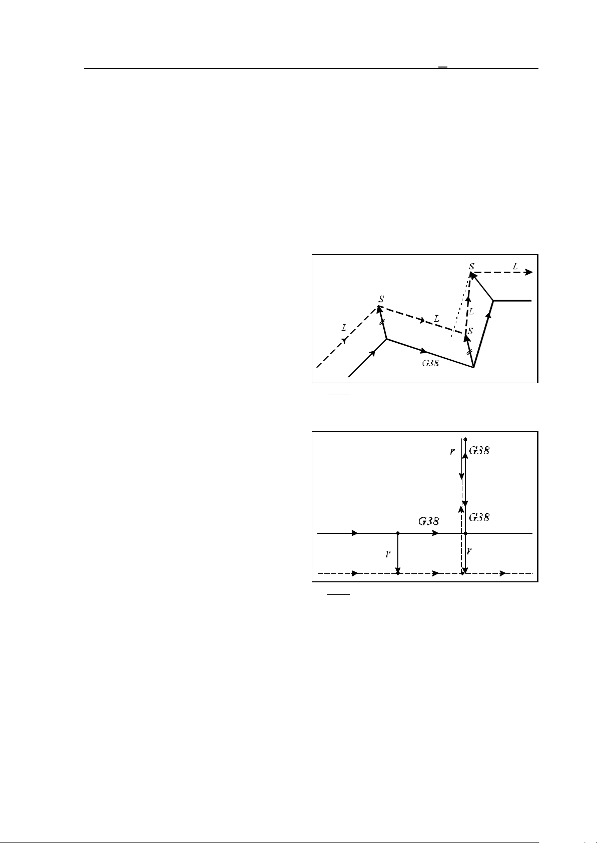
14 The Tool Compensation
14.5.5 Programming Vector Hold (G38)
Under the action of command
G38 v
the control will hold the last compensation vector between the previous interpolation and G38 block
in offset mode, and will implement it at the end of G38 block irrespective of the transition between
the G38 block and the next one. Code G38 is a single-shot one, i.e., it will not be modal.
G38 has to be programmed over again if the vector is to be held in several consecutive blocks.
G38 can be programmed in state G00 or G01 only, i.e., the vector-hold block must be invariably a
linear interpolation, or else the control will return error message 3040 G38 NOT IN G0, G1. Unless
code G38 is used in offset mode (G41, G42), the control will return error message 3039 G38
CODE IN G40.
An example of using G38:
...G17 G41 G91...
N110 G1 X60 Y60
N120 G38 X90 Y-40
N130 X20 Y70
N140 X60
...
Fig. 14.5.5-1
To program a recession without canceling the
offset mode:
...G17 G42 G91...
N110 G1 X40
N120 G38 X50
N130 G38 Y70
N140 G38 Y-70
N150 X60
...
Fig. 14.5.5-2
14.5.6 Programming Corner Arcs (G39)
By programming
G39 (I J K),
it will be possible - in offset mode - to avoid the automatic intersection-point computation or the
insertion of linear sections when going around outside corners, instead the tool center will travel
along a circular arc equal to the tool radius.
It will insert an arc equal to the tool radius in direction G02 or G03 in state G41 or G42,
respectively.
99
Page 100
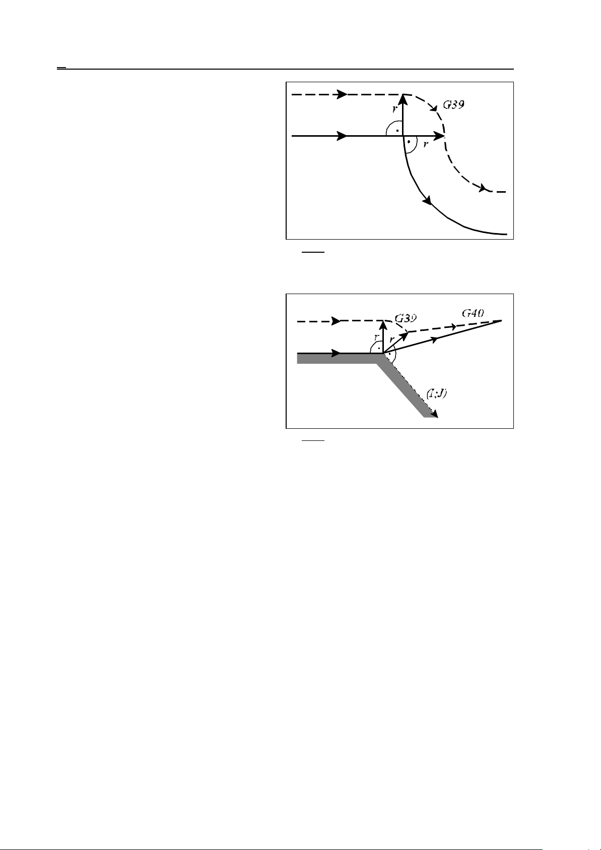
14 The Tool Compensation
The start and end points of the arc will be given
by a tool-radius long vector perpendicular to the
end point of the path of previous interpolation
and by a tool-radius vector perpendicular to the
start point of the next one, respectively. G39
has to be programmed in a separate block:
...G17 G91 G41...
N110 G1 X100
N120 G39
N130 G3 X80 Y-80 I80
...
When I, J or K is programmed in block G39,
the end point of the circular arc will be given by
a tool-radius long vector perpendicular to the
vector defined by I, J or K from the end point
of the previous interpolation, in accordance with
the selected plane.
...G17 G91 G41...
N110 G1 X100
N120 G39 I50 J-60
N130 G40 X110 Y30
...
Fig. 14.5.6-1
Fig. 14.5.6-2
The previously selected mirroring or rotating commands are effectual the vector defined by I, J or K.
As a matter of fact, the scaling command will not affect the direction. No movement command can
be programmed in a block of G39 type. The control will return error message 3036 G39 CODE IN
G40 if command G39 is issued in state G40 or 3D compensation mode.
100
 Loading...