National Instruments Order Analysis Toolset User Manual

Download

LabVIEW

Order Analysis Toolset User Manual

LabVIEW Order Analysis Toolset User Manual

August 2003 Edition

Part Number 322879B-01

Support

Worldwide Technical Support and Product Information

ni.com

National Instruments Corporate Headquarters

11500 North Mopac Expressway Austin, Texas 78759-3504 USA Tel: 512 683 0100

Worldwide Offices

Australia 1800 300 800, Austria 43 0 662 45 79 90 0, Belgium 32 0 2 757 00 20, Brazil 55 11 3262 3599, Canada (Calgary) 403 274 9391, Canada (Montreal) 514 288 5722, Canada (Ottawa) 613 233 5949, Canada (Québec) 514 694 8521, Canada (Toronto) 905 785 0085, Canada (Vancouver) 514 685 7530, China 86 21 6555 7838, Czech Republic 420 2 2423 5774, Denmark 45 45 76 26 00, Finland 385 0 9 725 725 11, France 33 0 1 48 14 24 24, Germany 49 0 89 741 31 30, Greece 30 2 10 42 96 427, India 91 80 51190000, Israel 972 0 3 6393737, Italy 39 02 413091, Japan 81 3 5472 2970, Korea 82 02 3451 3400, Malaysia 603 9131 0918, Mexico 001 800 010 0793, Netherlands 31 0 348 433 466, New Zealand 0800 553 322, Norway 47 0 66 90 76 60, Poland 48 0 22 3390 150, Portugal 351 210 311 210, Russia 7 095 783 68 51, Singapore 65 6226 5886, Slovenia 386 3 425 4200, South Africa 27 0 11 805 8197, Spain 34 91 640 0085, Sweden 46 0 8 587 895 00, Switzerland 41 56 200 51 51, Taiwan 886 2 2528 7227, Thailand 662 992 7519, United Kingdom 44 0 1635 523545

For further support information, refer to the Technical Support and Professional Services appendix. To comment on the documentation, send email to techpubs@ni.com.

Important Information

Warranty

The media on which you receive National Instruments software are warranted not to fail to execute programming instructions, due to defects in materials and workmanship, for a period of 90 days from date of shipment, as evidenced by receipts or other documentation. National Instruments will, at its option, repair or replace software media that do not execute programming instructions if National Instruments receives notice of such defects during the warranty period. National Instruments does not warrant that the operation of the software shall be uninterrupted or error free.

A Return Material Authorization (RMA) number must be obtained from the factory and clearly marked on the outside of the package before any equipment will be accepted for warranty work. National Instruments will pay the shipping costs of returning to the owner parts which are covered by warranty.

National Instruments believes that the information in this document is accurate. The document has been carefully reviewed for technical accuracy. In the event that technical or typographical errors exist, National Instruments reserves the right to make changes to subsequent editions of this document without prior notice to holders of this edition. The reader should consult National Instruments if errors are suspected. In no event shall National Instruments be liable for any damages arising out of or related to this document or the information contained in it.

XCEPT AS SPECIFIED HEREIN, NATIONAL INSTRUMENTS MAKES NO WARRANTIES, EXPRESS OR IMPLIED, AND SPECIFICALLY DISCLAIMS ANY WAR RANTY OF

MERCHANTABILITY OR FITNESS FOR A PARTICULAR PURPOSE . CUSTOMER’S RIGHT TO RECOVER DAMAGES CAUSED BY FAULT OR NEGLIGENCE ON THE PART OF

ATIONAL INSTRUMENTS SHALL BE LIMITED TO THE AMOUNT THERETOFORE PAID BY THE CUSTOMER. NATIONAL INSTRUMENTS WILL NOT BE LIABLE FOR DAMAGES RESULTING FROM LOSS OF DATA, PROFITS, USE OF PRODUCTS, OR INCIDENTAL OR CONSEQUENTIAL DAMAGES, EVEN IF ADVISED OF THE POSS IBILITY THEREOF. This limitation of the liability of National Instruments will apply regardless of the form of action, whether in contract or tort, including

negligence. Any action against National Instruments must be brought within one year after the cause of action accrues. National Instruments shall not be liable for any delay in performance due to causes beyond its reasonable control. The warranty provided herein does not cover damages, defects, malfunctions, or service failures caused by owner’s failure to follow the National Instruments installation, operation, or maintenance instructions; owner’s modification of the product; owner’s abuse, misuse, or negligent acts; and power failure or surges, fire, flood, accident, actions of third parties, or other events outside reasonable control.

Copyright

Under the copyright laws, this publication may not be reproduced or transmitted in any form, electronic or mechanical, including photocopying, recording, storing in an information retrieval system, or translating, in whole or in part, without the prior written consent of National Instruments Corporation.

Trademarks

LabVIEW™, National Instruments™, NI™, and ni.com™ are trademarks of National Instruments Corporation.

Product and company names mentioned herein are trademarks or trade names of their respective companies.

Patents

For patents covering National Instruments products, refer to the appropriate location: Help»Patents in your software, the patents.txt file on your CD, or

ni.com/patents.

WARNING REGARDING USE OF NATIONAL INSTRUMENTS PRODUCTS

(1) NATIONAL INSTRUMENTS PRODUCTS ARE NOT DESIGNED WITH COMPONENTS AND TESTING FOR A LEVEL OF RELIABILITY SUITABLE FOR USE IN OR IN CONNECTION WITH SURGICAL IMPLANTS OR AS CRITICAL COMPONENTS IN ANY LIFE SUPPORT SYSTEMS WHOSE FAILURE TO PERFORM CAN REASONABLY BE EXPECTED TO CAUSE SIGNIFICANT INJURY TO A HUMAN.

(2) IN ANY APPLICATION, INCLUDING THE ABOVE, RELIABILITY OF OPERATION OF THE SOFTWARE PRODUCTS CAN BE IMPAIRED BY ADVERSE FACTORS, INCLUDING BUT NOT LIMITED TO FLUCTUATIONS IN ELECTRICAL POWER SUPPLY, COMPUTER HARDWARE MALFUNCTIONS, COMPUTER OPERATING SYSTEM SOFTWARE FITNESS, FITNESS OF COMPILERS AND DEVELOPMENT SOFTWARE USED TO DEVELOP AN APPLICATION, INSTALLATION ERRORS, SOFTWARE AND HARDWARE COMPATIBILITY PROBLEMS, MALFUNCTIONS OR FAILURES OF ELECTRONIC MONITORING OR CONTROL DEVICES, TRANSIENT FAILURES OF ELECTRONIC SYSTEMS (HARDWARE AND/OR SOFTWARE), UNANTICIPATED USES OR MISUSES, OR ERRORS ON THE PART OF THE USER OR APPLICATIONS DESIGNER (ADVERSE FACTORS SUCH AS THESE ARE HEREAFTER COLLECTIVELY TERMED “SYSTEM FAILURES”). ANY APPLICATION WHERE A SYSTEM FAILURE WOULD CREATE A RISK OF HARM TO PROPERTY OR PERSONS (INCLUDING THE RISK OF BODILY INJURY AND DEATH) SHOULD NOT BE RELIANT SOLELY UPON ONE FORM OF ELECTRONIC SYSTEM DUE TO THE RISK OF SYSTEM FAILURE. TO AVOID DAMAGE, INJURY, OR DEATH, THE USER OR APPLICATION DESIGNER MUST TAKE REASONABLY PRUDENT STEPS TO PROTECT AGAINST SYSTEM FAILURES, INCLUDING BUT NOT LIMITED TO BACK-UP OR SHUT DOWN MECHANISMS. BECAUSE EACH END-USER SYSTEM IS CUSTOMIZED AND DIFFERS FROM NATIONAL INSTRUMENTS' TESTING PLATFORMS AND BECAUSE A USER OR APPLICATION DESIGNER MAY USE NATIONAL INSTRUMENTS PRODUCTS IN COMBINATION WITH OTHER PRODUCTS IN A MANNER NOT EVALUATED OR CONTEMPLATED BY NATIONAL INSTRUMENTS, THE USER OR APPLICATION DESIGNER IS ULTIMATELY RESPONSIBLE FOR VERIFYING AND VALIDATING THE SUITABILITY OF NATIONAL INSTRUMENTS PRODUCTS WHENEVER NATIONAL INSTRUMENTS PRODUCTS ARE INCORPORATED IN A SYSTEM OR APPLICATION, INCLUDING, WITHOUT LIMITATION, THE APPROPRIATE DESIGN, PROCESS AND SAFETY LEVEL OF SUCH SYSTEM OR APPLICATION.

About This Manual

How to Use This Manual ...............................................................................................vii

Conventions ...................................................................................................................vii

Related Documentation..................................................................................................viii

Chapter 1 Introduction to the LabVIEW Order Analysis Toolset

Overview of the LabVIEW Order Analysis Toolset......................................................1-1

Overview of the LabVIEW Order Analysis Start-Up Kit..............................................1-1

Important Considerations for the Analysis of Rotating Machinery...............................1-2

System Requirements ....................................................................................................1-3

Installation .....................................................................................................................1-3

Example VIs ..................................................................................................................1-4

Acquiring Data for Example VIs.....................................................................1-4

Configuring DAQ Hardware Used with Examples .........................................1-4

Acquire Data (Analog Tach) VI........................................................1-5

Acquire Data with PXI 4472 and TIO VI .........................................1-6

Chapter 2 Order Analysis

Order Analysis Definition and Application ...................................................................2-1

Order Analysis Basics....................................................................................................2-1

Effect of Rotational Speed on Order Identification .......................................................2-4

Constant Rotational Speed ..............................................................................2-4

Variable Rotational Speed...............................................................................2-6

Harmonic Analysis ..........................................................................................2-9

Order Analysis.................................................................................................2-9

Order Analysis Methods ................................................................................................2-9

Gabor Transform .............................................................................................2-10

Resampling ......................................................................................................2-13

Adaptive Filter.................................................................................................2-15

Contents

Chapter 3 Gabor Transform-Based Order Tracking

Overview of Gabor Order Analysis............................................................................... 3-1

Extracting the Order Components ................................................................................. 3-3

Masking .........................................................................................................................3-5

Extracting Orders ............................................................................................ 3-6

Reconstructing the Signal ............................................................................... 3-7

Displaying Spectral Maps.............................................................................................. 3-8

Calculating Waveform Magnitude ................................................................................ 3-10

Chapter 4 Resampling-Based Order Analysis

LabVIEW Order Analysis Toolset Resampling Method............................................... 4-1

Determining the Time Instance for Resampling ........................................................... 4-2

Resampling Vibration Data ........................................................................................... 4-4

Slow Roll Compensation............................................................................................... 4-5

Chapter 5 Calculating Rotational Speed

Digital Differentiator Method........................................................................................ 5-1

Averaging Pulses ........................................................................................................... 5-3

Appendix A Gabor Expansion and Gabor Transform

Appendix B References

Appendix C Technical Support and Professional Services

Glossary

Index

LabVIEW Order Analysis Toolset User Manual vi ni.com

About This Manual

This manual provides information about the LabVIEW Order Analysis Toolset, including system requirements, installation, and suggestions for getting started with order analysis and the toolset. The manual also provides a brief discussion of the order analysis process and the algorithm used by the LabVIEW Order Analysis Toolset.

How to Use This Manual

If you are just beginning to gain experience with order analysis, read Chapter 2, Order Analysis, of this manual and experiment with the Order Analysis Start-Up Kit. Refer to Chapter 1, Introduction to the

LabVIEW Order Analysis Toolset, for information about the Order

Analysis Start-Up Kit.

If you have experience with order analysis, use the example VIs to learn about how to use the LabVIEW Order Analysis Toolset. Refer to Chapter 1, Introduction to the LabVIEW Order Analysis Toolset, for information about the example VIs.

If you want to learn more about the algorithm used in the LabVIEW Order Analysis Toolset, refer to Chapter 3, Gabor Transform-Based Order

Tracking, and Chapter 4, Resampling-Based Order Analysis.

For information about individual VIs, refer to the Order Analysis Toolset Help, available in LabVIEW 6.1 by selecting Help»Order Analysis. In LabVIEW 7.0 and later, Order Analysis Toolset Help is part of the LabVIEW Help, which is available by selecting Help»VI, Function,

& How-To Help.

Conventions

The following conventions appear in this manual:

» The » symbol leads you through nested menu items and dialog box options

to a final action. The sequence File»Page Setup»Options directs you to pull down the File menu, select the Page Setup item, and select Options from the last dialog box.

This icon denotes a note, which alerts you to important information.

About This Manual

bold Bold text denotes items that you must select or click in the software, such

as menu items and dialog box options. Bold text also denotes the names of parameters, dialog boxes, sections of dialog boxes, windows, menus, palettes, and front panel controls and buttons.

italic Italic text denotes variables or cross references.

monospace Text in this font denotes text or characters that you should enter from the

keyboard, sections of code, programming examples, and syntax examples. This font is also used for the proper names of disk drives, paths, directories, programs, subprograms, subroutines, device names, functions, operations, variables, filenames and extensions, and code excerpts.

Platform Text in this font denotes a specific platform and indicates that the text

following it applies only to that platform.

Overview of the LabVIEW Order Analysis Toolset

The LabVIEW Order Analysis Toolset is a collection of virtual instruments (VIs) for LabVIEW. These VIs help you measure and analyze noise or vibration signals generated by rotating machinery by enabling you to perform the following analysis operations:

• Calculation and examination of rotational speed

• Measurement of the power distribution in the frequency domain or in the order domain as a function of either time or rotational speed

• Extraction of the order components from the original noise or vibration signal

• Measurement of the magnitude and phase of any order component as a function of rotational speed

• Presentation of data in a waterfall, orbit, or polar plot

The LabVIEW Order Analysis Toolset includes easy and advanced VIs. Use the easy VIs to perform simple tasks in just a few steps. The advanced VIs provide flexibility and increased control of the analysis process. Refer to the LabVIEW Order Analysis Toolset Help for information about individual VIs.

Overview of the LabVIEW Order Analysis Start-Up Kit

The Order Analysis Start-Up Kit is automatically installed when you install the LabVIEW Order Analysis Toolset. To open the Order Analysis Start-Up Kit, select Start»Programs»National Instruments»Order Analysis»Order Analysis Start-Up. The Order Analysis Start-Up Kit includes a LabVIEW application for order analysis. The order analysis

Chapter 1 Introduction to the LabVIEW Order Analysis Toolset

application is built with components found in the LabVIEW Order Analysis Toolset.

The order analysis application provides an example of how the LabVIEW Order Analysis Toolset can help you successfully complete analysis projects. The simple processes included in the order analysis application enable you to perform data acquisition, tachometer analysis, tachless speed profile generation, order analysis, and online monitoring of noise or vibration signals generated by rotating machinery. You also can use the order analysis application as a simple order analysis VI in projects or as a tool to learn the basics of building and using LabVIEW Order Analysis Tools e t VI s.

Important Considerations for the Analysis of Rotating Machinery

Order analysis is a powerful tool for analyzing rotating machinery when the rotational speed might change over time. However, to successfully use the LabVIEW Order Analysis Toolset, you must observe the following condition and restriction:

• Provide a signal directly related to the position of the shaft, such as a pulse train from a tachometer or key phasor. Although the LabVIEW Order Analysis Toolset can measure the magnitude of the order components without a tachometer signal, the measurement of the phase of the order components requires a tachometer signal.

• Do not use the LabVIEW Order Analysis Toolset for analysis of frequencies that are not excited by a fundamental frequency, such as the modes encountered in modal analysis. Although you can observe the different modes in the frequency domain, no simple relationship exists among those different modes. Usually, the frequencies of different modes are not simply a multiple of a fundamental frequency over time.

LabVIEW Order Analysis Toolset User Manual 1-2 ni.com

System Requirements

You must have LabVIEW 6.1 or later Full Development System or Professional Development System installed to run the LabVIEW Order Analysis Toolset.

Note Refer to the LabVIEW Release Notes for the required system configuration for

LabVIEW.

Note Order analysis is a memory-intensive task, especially when you display spectral

maps. Increasing the amount of RAM in your system can significantly increase system performance.

Installation

This section provides instructions for installing the LabVIEW Order Analysis Toolset.

Note Some virus detection programs interfere with the installer. Disable any automatic

virus detection programs before you install. After installation, check your hard disk for viruses and enable any virus detection programs you disabled.

Chapter 1 Introduction to the LabVIEW Order Analysis Toolset

(Windows 2000/NT/XP) Complete the following steps to install the LabVIEW

Order Analysis Toolset.

1. Log on as an administrator or as a user with administrator privileges.

2. Insert the LabVIEW Order Analysis Toolset 2.0 installation CD into the CD-ROM drive and follow the instructions that appear on the screen. If the startup screen does not appear, select Start»Run, navigate to the Toolset 2.0 installation CD, and double-click

(Windows Me/98) Insert the LabVIEW Order Analysis Toolset 2.0

installation CD and follow the instructions that appear on the screen. If the startup screen does not appear, select Start»Run, navigate to the folder on the LabVIEW Order Analysis Toolset 2.0 installation CD, and double-click

Setup folder on the LabVIEW Order Analysis

OAT.exe.

Setup

OAT.exe.

Chapter 1 Introduction to the LabVIEW Order Analysis Toolset

Example VIs

If you have experience with order analysis, the example VIs, located in the

examples\Order Analysis directory, can help you learn how to use

the LabVIEW Order Analysis Toolset. The example VIs illustrate the following LabVIEW Order Analysis Toolset functions for both analog and digital tachometer signal processing:

• Acquiring data

• Presenting data

• Gabor order tracking

• Resample order tracking

The example VIs use VIs found on the LabVIEW Order Analysis Toolset palettes and illustrate the basic capabilities of the LabVIEW Order Analysis Toolset.

Acquiring Data for Example VIs

For most of the example VIs, you can use prerecorded data or data you acquire with data acquisition (DAQ) hardware. The example VIs that accept either prerecorded data or acquired data have a Boolean control named Data Source. The Data Source control has two choices, Example and DAQ. When you choose Example, the VI uses prerecorded data generated during a fan run-up as the data source. When you choose DAQ, the VI uses data you acquire with DAQ hardware.

When acquiring data through DAQ hardware, National Instruments recommends you follow the following guidelines:

• Use an anti-aliasing filter before data acquisition to avoid the frequency alias.

• Sample the data from different channels simultaneously to maintain the phase relationship between channels, such as a tachometer signal and a vibration signal.

Configuring DAQ Hardware Used with Examples

The example VIs that accept both prerecorded data and acquired data use either an analog tachometer signal or a digital tachometer signal. The front panel of the example VI specifies the type of tachometer signal the VI uses, for example, Gabor Order Tracking (Analog Tach) or Gabor Order Tracking (Digital Tach). Depending on whether the example is an analog tachometer example or a digital tachometer example, when Data Source is

LabVIEW Order Analysis Toolset User Manual 1-4 ni.com

Chapter 1 Introduction to the LabVIEW Order Analysis Toolset

set to DAQ and you click the Run button on the front panel of the example VI, one of the following VIs opens:

• Acquire Data (Analog Tach) VI

• Acquire Data with PXI 4472 and TIO VI

Refer to the Acquire Data (Analog Tach) VI section for information about the Acquire Data (Analog Tach) VI and the Acquire Data with PXI 4472

and TIO VI section for information about the Acquire Data with PXI 4472

and TIO VI.

Acquire Data (Analog Tach) VI

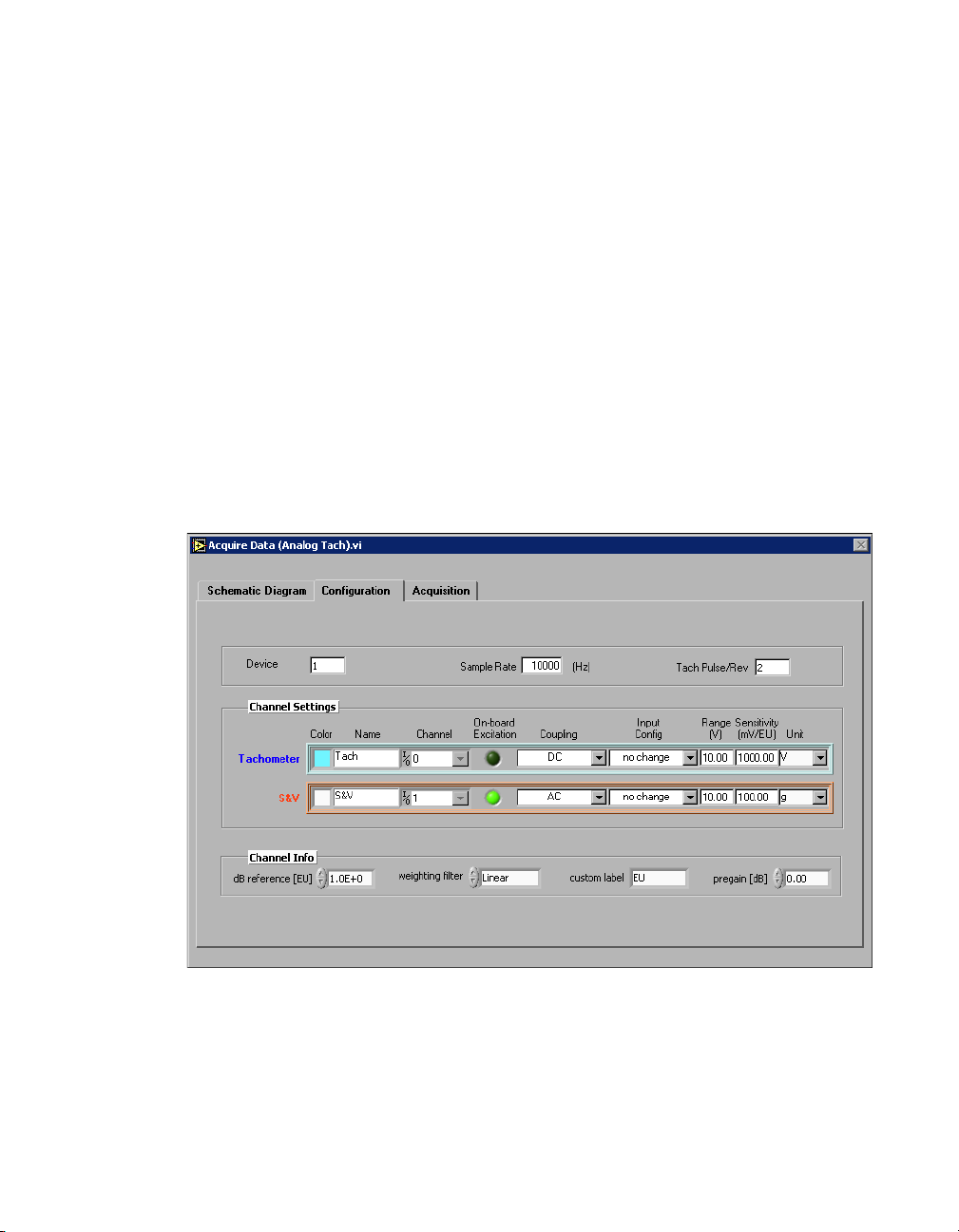
In analog tachometer examples, setting Data Source to DAQ and clicking the Run button opens the Acquire Data (Analog Tach) VI. The Acquire Data (Analog Tach) VI helps you acquire vibration data with a digital tachometer signal. Figure 1-1 shows the Configuration tab of the Acquire Data (Analog Tach) VI.

Figure 1-1. Acquire Data (Analog Tach) VI Configuration Tab

You must configure two channels of the DAQ device before you acquire data. Use the Configuration tab of the Acquire Data (Analog Tach) VI, shown in Figure 1-1, to configure your DAQ device. In the Channel Settings section of the Configuration tab, use Tachometer for the

Chapter 1 Introduction to the LabVIEW Order Analysis Toolset

tachometer signal and S&V for the sound or vibration sensor. After choosing data acquisition settings, enter the number of pulses you want the tachometer to generate per revolution in the Tach Pulse/Rev text box. Use the controls in the Channel Info section of the Configuration tab to specify the channel information for the sound or vibration sensor.

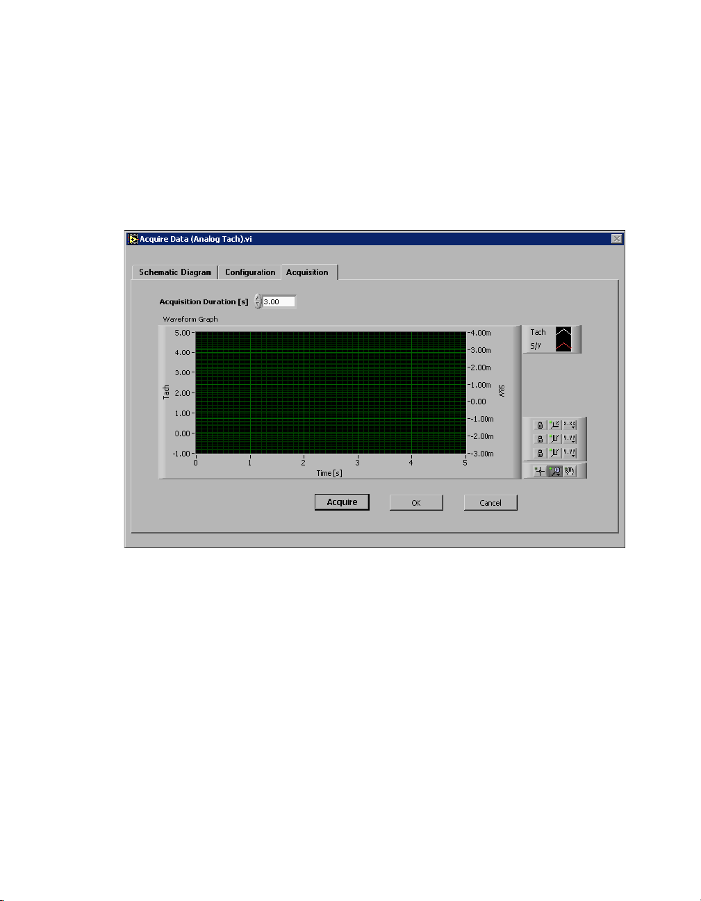
After configuring the DAQ device, click the Acquisition tab, shown in Figure 1-2.

Figure 1-2. Acquire Data (Analog Tach) VI Acquisition Tab

The Acquisition tab, shown in Figure 1-2, allows you to acquire and observe data. Click the Acquire button to acquire data. Continue to configure the data acquisition and acquire data until you acquire the data you want. Click the OK button to return to the front panel of the example VI to analyze the data.

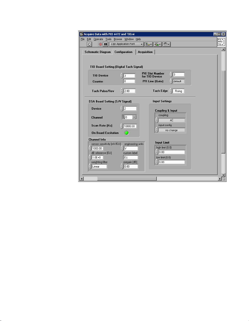
Acquire Data with PXI 4472 and TIO VI

In digital tachometer examples, setting Data Source to DAQ and clicking the Run button opens the Acquire Data with PXI 4472 and TIO VI. The Acquire Data with PXI 4472 and TIO VI helps you acquire vibration data with a digital tachometer signal. Figure 1-3 shows the Configuration tab of the Acquire Data with PXI 4472 and TIO VI.

LabVIEW Order Analysis Toolset User Manual 1-6 ni.com

Chapter 1 Introduction to the LabVIEW Order Analysis Toolset

Figure 1-3. Acquire Data with PXI 4472 and TIO VI Configuration Tab

Use the Configuration tab of the Acquire Data with PXI 4472 and TIO VI, shown in Figure 1-3, to configure the DAQ devices. Use one of the counters on a TIO device to receive TTL-compatible tachometer pulses. Use the controls in the TIO Board Setting (Digital Tach Signal) section of the Configuration tab to configure the TIO device. Use an NI PXI-4472 to acquire the data from the sound or vibration sensor. Use the controls in the DSA Board Setting (S/V Signal) and Input Settings sections of the Configure tab to configure the NI PXI-4472. 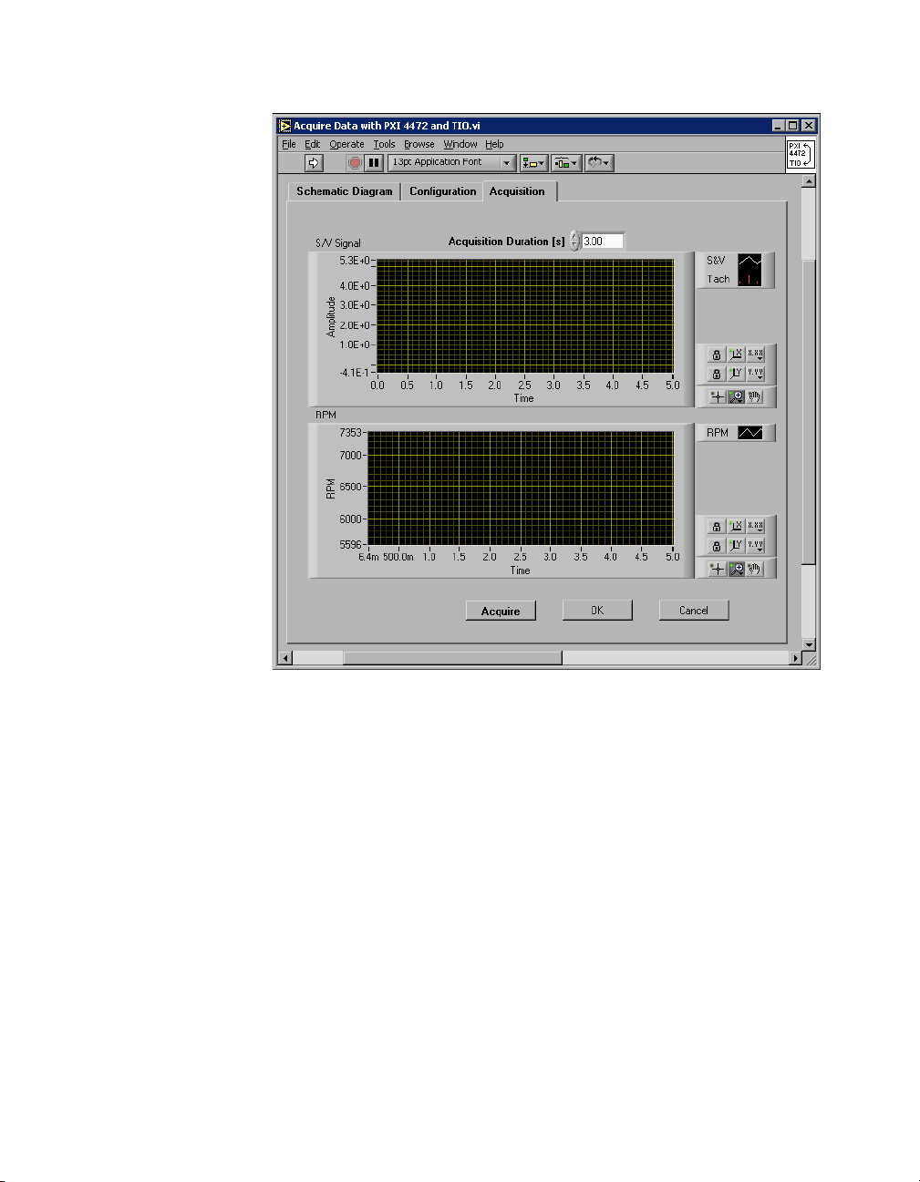After configuring the DAQ devices, click the Acquisition tab, shown in Figure 1-4.

Chapter 1 Introduction to the LabVIEW Order Analysis Toolset

Figure 1-4. Acquire Data with PXI 4472 and TIO VI Acquisition Tab

The Acquisition tab, shown in Figure 1-4, allows you to acquire and observe data. Click the Acquire button to acquire data. Continue to configure the data acquisition and acquire data until you acquire the data you want. Click the OK button to return to the front panel of the example VI to analyze the data.

LabVIEW Order Analysis Toolset User Manual 1-8 ni.com

Order Analysis

This chapter gives brief descriptions of the need for order analysis, the basic concepts of order analysis, the effect of rotational speed on order identification, and the different order analysis methods.

Order Analysis Definition and Application

When it is impossible or undesirable to physically open up a system and study it, you often can gain knowledge about the system by measuring and analyzing signals associated with the system. For example, physicists and chemists use the spectrum generated by a prism to distinguish between different types of matter. Astronomers apply spectra, as well as the Doppler effect, to determine distances between planets. Physicians use the electrocardiograph (ECG), which traces the electrical activity of the heart, as a nonsurgical means of diagnosing heart problems.

You can use order analysis to study, design, and monitor rotating machinery. By measuring and analyzing sound or vibration signals generated by a system with rotational components, you can gain a better understanding of the system, associate features of noise and vibration with the physical characteristics of the system, and identify system characteristics that change with time and operating conditions. Systems with rotational components include automobiles, airplanes, air conditioners, and PC hard drives.

Order Analysis Basics

Order analysis and harmonic analysis have much in common. The term harmonic refers to frequencies that are integer or fractional multiples of a fundamental frequency.

When dealing with rotating machinery, you often can hear noise and feel vibration created by the parts associated with the rotating components. Parts associated with rotating components include bearings, gears, and blades. Vibration of the rotating components creates noise and vibration signals. The machine rotational speed is the source of the noise and

Chapter 2 Order Analysis

vibration signals. The frequency-domain representations of noise and vibration behave as harmonics of the machine rotational speed.

In many industries, the harmonics related to the rotational speed are referred to as orders. The corresponding harmonic analysis is called order analysis. The harmonic at the same frequency as that of the rotational speed is the first

order; the harmonic at twice the frequency of the rotational speed is the second order and so on. Therefore, you can think of order analysis as an application of harmonic analysis for rotating machinery.

Figure 2-1 shows the relationship between frequency and order spectra.

1.7E+4

0.0E+0

VibrationTachometer

–1.9E+4

–2.5E+4

3.0E+6

2.0E+6

0.0 0.1 0.2 0.3 0.4 0.5 0.6 0.7 Time (s)

1.1E+3

0.0 0.1 0.2 0.3 0.4 0.5 0.6 0.7 Time (s)

Spectrum

Frequency

3.3E–2

0.0 100.0 200.0 300.0 400.0 500.0 Frequency (Hz)

3.0E+6

2.0E+6

Order

Spectrum

3.3E–2

0.0 2.0 4.0 6.0 8.0 10.0

Order

Figure 2-1. Order and Frequency Domain Display of a Shaft Rotating at 3,000 rpm

The top graph in Figure 2-1 shows a vibration signal from a machine running at 3,000 revolutions per minute (rpm). The rotational speed is computed from the tachometer signal, which is shown as the second graph in Figure 2-1. The frequency domain and order domain plots of the signal are shown in the third and fourth graphs, respectively, in Figure 2-1.

LabVIEW Order Analysis Toolset User Manual 2-2 ni.com

Chapter 2 Order Analysis

Assuming that speed remains constant during data acquisition, you can use the following equations to switch between the frequency domain and the order domain.

RPM

Frequency

Order Frequency

-------------

Order×=

×=

-------------

RPM

Orders often reflect the physical characteristics of rotating machines. As in classical harmonic analysis, by analyzing the phase and amplitude relationships between different orders, you often can discover a great deal about the system in which you are interested. For example, order analysis has enabled the observation of the following relationships:

• Imbalance results in a spectral peak at the first order.

• Misalignment or bending of the shaft generates a large second order.

• Oil whirl might lead to strong fractional orders.

• Gears, belts, and blades might enhance high orders.

Figure 2-2 shows the order spectrum of the vibration signal measured from a PC fan with seven blades and four coils.

4 Coils 7 Blades

0.0 2.0 4.0 6.0 8.0 10.0

Orders

Figure 2-2. Order Spectrum of a PC Fan with Seven Blades and Four Coils

12.0 14.0 16.0

The vibration signal depicted in Figure 2-2 contains strong fourth and seventh orders. The four coils inside the fan drag and push the shaft four times per revolution, causing the strong fourth order. The seven blades of the fan pass the position of the sensor seven times per revolution and cause the strong seventh order.

Chapter 2 Order Analysis

Like classical harmonic analysis, order analysis is a powerful tool for gaining a better understanding of the condition of rotating machinery. However, compared to harmonic analysis, order analysis is more effective for the analysis of rotating machinery because you can use order analysis when a machine runs at a constant speed and when the rotational speed varies. As described in the Effect of Rotational Speed on Order Identification section, harmonic analysis is effective only when the rotational speed remains constant.

Effect of Rotational Speed on Order Identification

The ability to make a reliable identification of individual orders from the conventional power spectrum depends on whether rotational speed remains constant or varies. This section discusses the effect rotational speed has on the conventional power spectrum and discusses classical harmonic analysis and order analysis in relation to rotational speed.

Constant Rotational Speed

At a constant rotational speed, you can identify orders from both the conventional power spectrum and the frequency-time spectral map. Figure 2-3 illustrates the analysis of a vibration signal acquired from a PC fan running at a constant speed.

LabVIEW Order Analysis Toolset User Manual 2-4 ni.com

570

500

450

400

350

300

250

200

Frequency (Hz)

150

100

Chapter 2 Order Analysis

STFTSpectrum

31.9 31.9 31.9

Figure 2-3. PC Fan Running at Constant Speed

The bottom plot in Figure 2-3 depicts the tachometer pulses and the signal from an accelerometer mounted on the PC fan. The plot on the left in Figure 2-3 illustrates a conventional power spectrum based on the fast Fourier transform (FFT). The upper-right plot in Figure 2-3 shows the frequency-time spectral map computed from the short-time Fourier transform (STFT) with a 1,024-point Hanning window. Because of the constant rotational speed of the fan during data acquisition, you can identify several peaks in both the power spectrum and the frequency-time spectral map. The peaks indicate different orders and appear in the frequency-time spectral map as white lines.

Chapter 2 Order Analysis

Variable Rotational Speed

In addition to testing rotating machinery running at a constant speed, researchers often perform tests involving run-up and run-down. Like a swept-sine stimulus, testing run-up and run-down provides a stimulus over a wide range of frequencies.

According to Fourier analysis theory, the frequency bandwidth of a signal is proportional to the change in the frequency and amplitude of the signal. The faster the frequency changes, the wider the overall frequency bandwidth becomes, as measured from the power spectrum.

Figure 2-4 illustrates a conventional power spectrum on the left and the frequency-time spectral map on the right for a signal with constant frequency and amplitude.

Spectrum Frequency-Time Spectral Map

0.5

0.4

0.3

0.2

Frequency

0.1

0.0 Time Waveform

1.0

0.5

0.0

–0.5

–1.0

0 50 100 150 200 255

Time

Figure 2-4. Constant Frequency

In Figure 2-4, the overall frequency bandwidth is proportional to the change in frequencies. When the frequency and amplitude are constant over

LabVIEW Order Analysis Toolset User Manual 2-6 ni.com

time, the overall frequency bandwidth, as measured from the conventional power spectrum, is the minimum.

Figure 2-5 depicts a signal whose frequency changes as a function of time.

Spectrum Frequency-Time Spectral Map

0.5

0.4

0.3

0.2

Frequency

0.1

0.0 Time Waveform

1.0

0.5

0.0

–0.5

–1.0

0 50 100 150 200 255

Chapter 2 Order Analysis

Overall Bandwidth Becomes Wide as the Frequency Changes

Time

Figure 2-5. Frequency Changes Over Time

Although the signals in Figures 2-4 and 2-5 have similar frequency bandwidths at each time instant, the overall frequency bandwidths shown in their corresponding power spectra are rather different. As you can see from the two FFT-based power spectra in Figures 2-4 and 2-5, the overall frequency bandwidth of the signal whose frequency increases with time in Figure 2-5 is much wider than that of the signal whose frequency is constant in Figure 2-4. When frequency or amplitude vary with time, the corresponding overall frequency bandwidth, as measured from the conventional power spectrum, becomes wide.

When the frequency bandwidth of the fundamental component widens, the bandwidths of the associated harmonics also widen. The widening of the bandwidths of the harmonics eventually causes the frequency bandwidth of the harmonics to overlap in the conventional power spectrum. When the

Chapter 2 Order Analysis

harmonics overlap in the conventional power spectrum, you are unable to identify different harmonics by using the conventional power spectrum.

Figure 2-6 shows the signal from the same PC fan as the one depicted in Figure 2-3. However, in Figure 2-6, the rotational speed of the fan increases with time.

1500

1250

1000

750

Frequency (Hz)

500

250

STFTSpectrum

31.9 31.9 31.9

Time (sec.)

Figure 2-6. Fan Run-Up

In Figure 2-6, as the rotational speed increases, both the fundamental frequency bandwidth and the frequency bandwidths of related orders widen, causing orders to overlap. Whether you can separate nearby orders in a power spectrum depends on the rate of change in the rotational speed, the window used, and the highest order of interest. In Figure 2-6, the power spectrum is measured over the entire duration of the fan run-up and does not really show any distinguishable orders. When the change of speed is large enough, the spectra of orders eventually overlap. When the spectra of

LabVIEW Order Analysis Toolset User Manual 2-8 ni.com

Harmonic Analysis

Order Analysis

Chapter 2 Order Analysis

orders overlap, you are unable to derive meaningful information about the individual orders.

Harmonic analysis is suitable for the analysis of rotating machinery only when the rotational speed remains constant. In classical harmonic analysis, the fundamental frequency does not change over time. Although the phases and amplitudes of the individual harmonics can vary over time, the center frequencies of all the harmonics remain constant.

When using the Fourier transform, you obtain the best results with the machine running at a constant rotational speed while taking measurements. If you want to take measurements at a different rotational speed, you have to run the machine to that rotational speed and take another measurement. Testing with discrete rotational speed increments is time consuming. Testing with discrete rotational speed increments also can be inaccurate or impossible if you cannot control the rotational speed of the system well or the system is not allowed to run at the critical rotational speed for a sufficient length of time.

An important goal of order analysis is to uncover information about the orders that might become buried in the power spectrum due to a change in rotational speed. While the orders are hidden in the overall power spectrum in Figure 2-6, the orders have distinguishable features in the frequency-time spectral map. The observation that orders have distinguishable features in the frequency-time spectral map serves as the starting point for uncovering information about orders that are difficult to see in the power spectrum.

Order Analysis Methods

The basic technique of order analysis involves obtaining the instantaneous speed of the rotating shaft of a machine from a tachometer or encoder signal. The speed is then correlated to the noise or vibration signal produced by the machine to obtain information about the order components, such as waveforms, magnitudes, and phases. In order analysis, revolutions, rather than time, serve as the basis for signal analysis. Thus, in the spectrum domain, the focus is on orders instead of frequency components.

Chapter 2 Order Analysis

Gabor Transform

Currently, the following methods generally are used to perform order analysis:

• Gabor transform

• Resampling

• Adaptive filter

The LabVIEW Order Analysis Toolset provides the Gabor-transform-based method and the resampling method of order analysis.

The Gabor transform is one of the invertible joint time-frequency transforms. With invertible joint time-frequency transforms, you can recover any time-domain input signal or an approximation of the signal by applying an inverse transform to the transform of the signal. The Gabor transform result is called a Gabor coefficient. The inverse Gabor transform is known as the Gabor expansion. You can think of the Gabor transform as a specific STFT. Even though you can recover a signal from its Gabor transform by using a Gabor expansion, you cannot reconstruct the general STFT using an inverse Fourier transform.

You can compute the Gabor transform by either STFT or windowed Fourier transform. However, to ensure reconstruction of the signal, you have to carefully manage the ratio of the analysis window to the window shift step and the capture of information at signal edges. Use the following methods to ensure reconstruction of the signal.

• Make sure that the ratio between the length of the analysis window and the window shift step is greater than or equal to 1. The ratio between the length of the analysis window and the window shift step determines the time overlap. By default in the LabVIEW Order Analysis Toolset, the ratio is set to 4. For example, if the window length is 2,048, the window shift is 512.

• Move the analysis window in such way that no information is missed, especially at the beginning and the end of the data samples. Zero padding and wrap padding are two commonly used methods for dealing with the edge data. Figure 2-7 illustrates zero padding and wrap padding.

LabVIEW Order Analysis Toolset User Manual 2-10 ni.com

Chapter 2 Order Analysis

Windows

Data Blocks

Zeros 1 2 n–1 n Zeros

(a) Zero Padding

Windows

Data Blocks

n–1 n 1 2

In zero padding, shown in Figure 2-7(a), the first window and the last window only cover one data block each. The remaining area in the range of the window is filled with zeros. Thus, extra data samples are added. After Gabor expansion, the reconstructed data is longer than the original data.

To avoid the reconstructed data being longer than the original data, consider the signal as periodic and use wrap padding, shown in Figure 2-7(b). In wrap padding, when the first few data blocks are analyzed, data blocks at the end of the data samples are wrapped ahead to fill the windows. You also can wrap data blocks backward from the beginning of the data sample to the end.

n–1 n 1

(b) Wrap Padding

Figure 2-7. Padding Schemes

Chapter 2 Order Analysis

0.4

0.2

0.0

–0.2

Amplitude

–0.4

–384 –300 –200 –100 128 8064 8200 8300 8400 8500 8576

0.4

0.2

0.0

–0.2

Amplitude

–0.4

–256 –100 0 200 7808 7900 8000 8100 8200 8320

Figure 2-8 shows two examples of padding.

Time

(a) Zero Padding

100 256

Time

(b) Wrap Padding

Figure 2-8. Padding Examples

Refer to Appendix A, Gabor Expansion and Gabor Transform, for more information about the Gabor transform and the Gabor expansion.

Refer to Chapter 3, Gabor Transform-Based Order Tracking, for information about how the LabVIEW Order Analysis Toolset uses a method based on the Gabor transform for order tracking.

LabVIEW Order Analysis Toolset User Manual 2-12 ni.com

Resampling

Chapter 2 Order Analysis

Resampling is a widely used method of order analysis. Figure 2-9 illustrates the resampling method.

Sample at Constant Time Frequency

Sample at Constant Angle Order

Figure 2-9. Resampling

In the resampling method, time-samples are converted to angle samples. The time-samples are samples of the physical signal that are equally spaced in time. The angle samples are samples that are equally spaced in the rotation angle.

You can acquire angle samples with either hardware or software. The hardware solution uses an encoder or a multiplied tachometer signal to trigger the analog-to-digital conversion, which ensures a sampling process spaced equally in the rotation angle. The hardware solution requires additional hardware devices and a tracking anti-aliasing filter.

Software programs designed to acquire angle samples complete the following steps to acquire the angle samples.

1. Collects the measured signal and the tachometer signal at some constant rate.

2. Uses interpolation or curve fitting to determine the instantaneous shaft angle at intermediate points between the tachometer pulses.

3. Calculates the sampling time at the desired shaft-angular increment.

4. Uses interpolation to obtain new samples at the desired time.

Chapter 2 Order Analysis

After acquiring angle samples with either hardware or software, you can perform a Fourier transform on the angle samples to analyze them. Because the time domain has changed into the angle domain, the frequency domain now becomes the order domain. You can separate and observe the order components through either the STFT spectrum or the order spectrum, which is actually the FFT spectrum.

Figure 2-10 shows the spectrum of angle samples.

Order

Order Spectrum

Order vs. Rev

Angle Samples

1.0

0.5

0.0

Amplitude

–0.5

–1.0

0 200 400 600 800 1000 1200 1400

Revolution

Figure 2-10. Spectrum of Angle Samples

In Figure 2-10, the Angle Samples plot shows the signal sampled at a constant angle-interval. The Order Spectrum plot shows the order spectrum obtained by performing a FFT on the angle samples. In the Order Spectrum plot, significant peaks appear at each order. The Order vs. Rev plot shows the result of a STFT on the angle samples, where an order axis is used instead of a frequency axis. Each horizontal white line in the Order vs. Rev plot indicates the strong power at an integer order.

LabVIEW Order Analysis Toolset User Manual 2-14 ni.com

Adaptive Filter

Chapter 2 Order Analysis

After the resampling process takes place, recovering a time waveform at a specific order might be difficult.

Refer to Chapter 4, Resampling-Based Order Analysis, for information about how the LabVIEW Order Analysis Toolset uses software-based resampling for order analysis.

Although the frequencies of the order components change as the rotational speed changes, you can consider the rotational speed and the frequency of order components to remain constant in a relatively short time interval. The adaptive filter method of order analysis filters out the desired order by using a bandpass filter whose passband frequency shifts according to the rotational speed.

The Vold-Kalman Order Tracking Filter is an example of the successful application of the adaptive filter method. With an accurate instantaneous speed signal as a guide, the Vold-Kalman Order Tracking Filter can extract, without ambiguity, two orders that are in close proximity to each other.

Gabor Transform-Based Order Tracking

This chapter discusses a new order analysis method based on the Gabor transform and provided by the LabVIEW Order Analysis Toolset that enables you to complete the following tasks:

• Analyze the order components of a noise or vibration signal

• Reconstruct the desired order components in the time domain

Overview of Gabor Order Analysis

The Gabor transform can give the power distribution of the original signal as the function of both time and frequency. Figure 3-1 shows a frequency-time spectral map computed by performing a Gabor transform on a sample vibration signal from a rotating machine.

500

450

400

350

300

250

200

Frequency (Hz)

150

100

0124681012357911131415

Time (s)

Figure 3-1. Frequency-Time Spectral Map of a Vibration Signal

Chapter 3 Gabor Transform-Based Order Tracking

In Figure 3-1, the magnitudes of coefficients are shown as gray scale, with full white indicating a maximal magnitude and full black indicating a minimal magnitude.

Because the rotational speed changes little in each time portion of the frequency-time spectral map, the spectrum of each order is clearly distinguishable. As the rotational speed varies over time, the frequency of one certain order component changes. Thus, the order component forms a curve with a large magnitude in the frequency-time spectral map, as shown in Figure 3-1. The white curves have magnitudes larger than the magnitudes in local neighborhoods off the curves. The white curves indicate the order components and are referred to as order curves.

From the frequency-time spectral map, you can separate the order curves, or any other part of the signal in which you are interested, from the intact original signal. You then can use Gabor expansion to reconstruct time waveforms of the orders.

Figure 3-2 illustrates the Gabor order analysis process provided by the LabVIEW Order Analysis Toolset.

Step 1:

Data

Acquisition

Vibration

Signal

Tachometer

Signal

Step 2:

Gabor

Transform

Step 3:

Tachometer

Processing

Gabor

Coefficients

Step 5:

Mask

Operation

Step 4: Display

2D Spectral

Map

Modified

Coefficients

Figure 3-2. Gabor Order Analysis Diagram

Step 6:

Gabor

Expansion

Order

Wavefo rm

Step 7:

Compute Magnitude and Phase

LabVIEW Order Analysis Toolset User Manual 3-2 ni.com

Chapter 3 Gabor Transform-Based Order Tracking

Complete the following steps to perform Gabor order analysis.

1. Acquire data samples from the tachometer and noise or vibration sensors synchronously at some constant sample rate.

2. Use the LabVIEW Order Analysis Toolset VIs to complete the following steps.

a. Perform a Gabor transform on the noise or vibration samples to

produce an initial Gabor coefficient array.

b. Calculate the rotational speed from the tachometer signal. Refer to

Chapter 5, Calculating Rotational Speed, for information about calculating rotational speed.

c. Generate a 2D spectral map from the initial coefficient array to

observe the whole signal over frequency-time, frequency-rpm, order-rpm, or rpm-order.

d. Generate a modified coefficient array, based on the rotational

speed and the order of interest, from the initial array by performing a masking operation.

e. Generate a time domain signal from the modified coefficient array

by performing Gabor expansion.

f. Calculate the waveform magnitude and phase.

Refer to the Important Considerations for the Analysis of Rotating

Machinery section of Chapter 1, Introduction to the LabVIEW Order Analysis Toolset, for information about a condition and restriction for using

the LabVIEW Order Analysis Toolset to analyze rotating machinery.

Extracting the Order Components

After generating the initial Gabor coefficient array through a Gabor transform, you can select one or more order components for analysis. You can convert the coefficient corresponding to the selected order component back into a time domain signal. The resulting time domain signal contains information only about the selected order component.

You select order components by including the coefficients along the corresponding order curves. Therefore, you must determine the position index of the coefficient on each order curve. Because the frequency of an order component is an integer or fractional multiple of the fundamental frequency, such as the rotational speed, the position index of a given order curve at each time interval is calculated by multiplying the order number and the fundamental frequency index at the time interval. If a signal is

Chapter 3 Gabor Transform-Based Order Tracking

processed by a Gabor transform, the index of the nth order is given by the following equation.

500–

400–

300–

200–

Frequency (Hz)

100–

index round

RPM



-------------



----

n××

where RPM is the averaged instantaneous rotational speed in the time interval, N is the number of frequency bins, and f

is the sampling

frequency. In the LabVIEW Order Analysis Toolset, the number of frequency bins N equals the length of the window.

Each order component in the order domain, as well as each harmonic in the frequency domain, has a side band. Thus, in the joint time-frequency domain, each order component contains the coefficients along the order curve and some coefficients in the neighborhood. You must include the coefficients in the neighborhood when selecting the order component.

Constant frequency bandwidth and constant order bandwidth are two ways to define the bandwidth of the neighborhood for an order curve. Figure 3-3 illustrates constant frequency bandwidth and constant order bandwidth.

500–

400–

300–

200–

Frequency (Hz)

100–

0–

0 5 25 30 3510 15 20 39

Time (s)

(a) Constant Frequency Bandwidth

Figure 3-3. Constant Frequency Bandwidth and Constant Order Bandwidth

0–

0 5 25 30 3510 15 20 39

Time (s)

(b) Constant Order Bandwidth

Figure 3-3(a) illustrates constant frequency bandwidth. The neighborhood

RPM

is considered as the region between and , where

-------------

∆

-----+ n

RPM

-------------

∆

-----–

∆ f is a constant frequency. The frequency of the bandwidth ∆ f remains

constant over time.

LabVIEW Order Analysis Toolset User Manual 3-4 ni.com

Chapter 3 Gabor Transform-Based Order Tracking

Figure 3-3(b) illustrates constant order bandwidth. The neighborhood is

Masking

RPM

considered as the region between and .

While the frequency bandwidth varies in time, the order bandwidth





RPM

-------------

× n

---+

 

RPM

-------------

---–

k remains constant.

You can use the Gabor Order Analysis VIs to determine the frequency bandwidth or order bandwidth automatically or in response to your input. For example, you can automatically determine a bandwidth for the time-frequency neighborhood based on an estimate of minimum order-distance to nearest neighbor order-components. Normally, the bandwidth should not exceed the distance between two nearby orders, which is the fundamental frequency, or first order.

After you determine the coefficient positions and the bandwidth of the selected order curves, select a subset of the initial Gabor coefficient array. The subset of the initial Gabor coefficient array contains only the coefficients in the neighborhood of the selected order curves. You can generate the subset by performing a mask operation on the initial Gabor coefficient array.

To perform the mask operation, you must construct a mask array. The mask array is a 2D array the same size as the coefficient array. However, the mask array contains only Boolean elements. When masking is performed, the coefficients at value TRUE are kept unchanged, while the coefficients at value FALSE are set to zero. The following equation represents the mask operation.



where c

is the original coefficient array, is the masked coefficient

m, n

array, and mask



mn,

is the mask array.

m, n

0 mask



mn,

mask

TRUE=

mn,

FALSE=

mn,

You can build a mask array according to the order number you want to analyze. In each row, elements within the bandwidth of the designated order number are set to either TRUE or FALSE. Use the Template to Mask

Chapter 3 Gabor Transform-Based Order Tracking

VI to perform the mask operation. Refer to the LabVIEW Order Analysis Toolset Help for information about the Template to Mask VI.

You can consider the mask operation a time-variant bandpass filter in the joint time-frequency domain. The center frequency of the passband equals the frequency of the order curve. The number of elements set to TRUE determines the bandwidth of the passband.

Extracting Orders

Figure 3-4 illustrates the order extraction and signal reconstruction process.

500–

400–

300–

200–

Frequency (Hz)

100–

0–

02 468101215 02 468101215

Time (s) Time (s)

(a) Original Signal (b) Mask

500–

400–

300–

200–

Frequency (Hz)

100–

0–

Time (s) Time (s)

500–

400–

300–

200–

Frequency (Hz)

100–

0–

500–

400–

300–

200–

Frequency (Hz)

100–

0–

02 46810121502 468101215

Reconstructed Signal

Figure 3-4. Gabor Coefficients

Figure 3-4(a) shows a frequency-time spectral map after the Gabor transform.

LabVIEW Order Analysis Toolset User Manual 3-6 ni.com

Figure 3-4(b) shows a mask array around the fourth order with a constant frequency bandwidth. The TRUE values comprise the white area, while the FALSE values comprise the black areas.

Figure 3-4(c) shows the masked coefficients. The black areas indicate values set to zero and correspond to the FALSE values in the mask array. The white area contains values copied from the original coefficient array and corresponds to the TRUE values in the mask array.

Figure 3-4(d) shows the frequency-time spectral map of the reconstructed signal.

Reconstructing the Signal

Figure 3-5 shows the fourth-order time waveform that was reconstructed by performing a Gabor expansion on the masked coefficients from Figure 3-4.

1.0–

)

0.5–

0.0–

Chapter 3 Gabor Transform-Based Order Tracking

Extracted 4th Order

Original Signal

–0.5–

Vibration (m/s

–1.0–

10.0 12.04.00.0 2.0 6.0 8.0 14.6

Time (s)

Figure 3-5. Original Signal and Extracted Order Component

Unlike the reverse discrete Fourier transform, the Gabor expansion, in general, is not a one-to-one mapping. A Gabor coefficient is the subspace of a two-dimensional function. An arbitrary two-dimensional function, such as the masked coefficient array, might not have a corresponding time waveform. Usually, the Gabor coefficients of the reconstructed time waveform are not exactly the same as the desired coefficients you mask. However, in terms of the least mean square error (LMSE), the Gabor coefficients of the reconstructed time waveform are the coefficients closest to the desired coefficients you mask.

Like conventional time-invariant filters, the time-variant filters implemented by the Gabor expansion have a certain passband and attenuation. The extracted time waveform is only a part of the original signal whose frequencies fall into the passband determined by the Gabor

Chapter 3 Gabor Transform-Based Order Tracking

time-variant filters. Figure 3-6 shows an original signal and the spectrum of the reconstructed signal.

–49.1–

–100.0–

–150.0–

–179.0–

Original Signal

Reconstructed Order

Expected Pass Band

250 300 3501000 50 150 200 408

Frequency (Hz)

Figure 3-6. Spectrum of Reconstructed Signal

In Figure 3-6, one row is selected from the joint time-frequency coefficient array. The selected row is nothing more than a windowed FFT power spectrum in the time interval. The original Gabor coefficients comprise the solid line in Figure 3-6. When performing a mask operation, coefficients outside the expected passband are set to zero.

After reconstruction, the spectrum of the reconstructed signal is formed. In Figure 3-6, the dashed line represents the spectrum of the reconstructed signal. Within the passband, the reconstructed signal keeps the same magnitude as the original signal. While outside the passband, the magnitude of the reconstructed signal is no longer zero. Instead, the magnitude does have some certain value. However, the value of the magnitude quickly decreases as the frequency leaves the passband.

Displaying Spectral Maps

Before extracting order components from the joint time-frequency domain, you might want to identify the order components in which you are most interested, such as which order is the most significant or which order contributes the most at a certain rotational speed. However, by using order extraction and reconstruction, you might have to process a large number of order components before you can obtain this information.

The LabVIEW Order Analysis Toolset provides several methods of obtaining a 2D spectral map over the whole signal in the frequency-time, frequency-rpm, and order-rpm domains. Figure 3-7 shows the three types of spectral maps for a vibration signal.

LabVIEW Order Analysis Toolset User Manual 3-8 ni.com

Chapter 3 Gabor Transform-Based Order Tracking

5000

4000

3000

2000

1000

0 5 10 15 20 25 30 36 0.0 5.0 10.0 15.0 20.0 25.0 30.0 36.0

Time (s)

5000

4000

3000

2000

Frequency Frequency

1000

(a) Frequency-Time Spectral Map

991 1250 1500 1750 2000 2250 2500 2774

RPM

3000

2500

2000

1500

1000

500

Time (s)

(b) RPM vs. Time

150

125

100

Order RPM

991 1250 1500 1750 2000 2250 2500 2774

RPM

(d) Order-RPM Spectral Map

Figure 3-7. 2D Spectral Maps

Figure 3-7(a) is the frequency-time spectral map generated directly from the Gabor coefficients. The magnitudes of coefficients are shown as gray scale, with full white indicating a maximal magnitude and full black indicating a minimal magnitude. Order components are shown as curves. Because the frequency of each order component shifts as the rotational speed varies over time, the outline of each curve is similar to the rpm-time function shown in Figure 3-7(b).

In Figure 3-7(a), notice the horizontal white lines. The horizontal white lines indicate the large power around the resonance frequencies. The physical characteristics of the system containing the rotating machinery determine the resonance frequency. The resonance frequency does not change as the rotational speed changes.

Chapter 3 Gabor Transform-Based Order Tracking

Figure 3-7(c) shows the frequency-rpm spectral map. The horizontal axis represents rpm, or rotational speed. You can map the rpm axis from the time axis in the frequency-time spectral map by the rpm-time function. The frequency of each order component is calculated by the following equation.

Because the relationship between rpm and frequency is a linear function,

order components appear as lines with a slope of in Figure 3-7(c).

The resonance beams appear as horizontal lines.

Applying a frequency-to-order-number transform to the frequency-rpm spectral map generates the order-rpm spectral map, shown in Figure 3-7(d). The order-rpm spectral map displays the order components as horizontal lines and the resonance beams as hyperbolas.

Using the frequency-time spectral map, the frequency-rpm spectral map, and the order-rpm spectral map, you can clearly and efficiently observe all the order components in the entire time and rpm ranges.

Frequency

RPM

-------------

Order×=

RPM

-------------

Calculating Waveform Magnitude

The reconstructed time waveform of the selected order contains only a few frequency components in a relatively short time interval. Therefore, the reconstructed time waveform of the selected order displays like a sine waveform in which the frequency and magnitude have been modulated.

In practical applications such as product testing for comparison with reference curves, calculating the waveform magnitude as a function of rpm is useful. The LabVIEW Order Analysis Toolset uses the root mean square (RMS) of the time waveform to calculate the waveform magnitude and correlate the sine waveform with the tachometer pulses to obtain the waveform phase. Both the magnitude and the phase are computed in a short time interval. By means of the time-rpm function, the LabVIEW Order Analysis Toolset performs a time-to-rpm mapping operation to obtain the waveform magnitude and phase as a function of rpm.

LabVIEW Order Analysis Toolset User Manual 3-10 ni.com

Resampling-Based Order Analysis

This chapter describes the resampling method provided by the LabVIEW Order Analysis Toolset, determining the time instance for resampling, resampling vibration data, and slow roll compensation.

LabVIEW Order Analysis Toolset Resampling Method

With software resampling, the LabVIEW Order Analysis Toolset enables you to complete the following tasks:

• Resample even time-space samples to even angle-spaced samples

• Obtain magnitude and phase information for each order

Figure 4-1 illustrates the resampling-based order analysis process provided by the LabVIEW Order Analysis Toolset.

Tachometer

Signal

Step 1:

Data

Acquisition

Vibration

Signal

Step 2:

Determine the

Time Instant

for Resampling

Time

Instant

Step 3:

Resample the Vibration Data

Step 4(a):

Compute

Order

Spectrum

Step 4(b):

Track Magnitude

Resampled

Signal

Figure 4-1. Resampling-Based Order Analysis Diagram

and Phase of

Individual Orders

Magnitude and Phase

Step 5:

Slow Roll

Compensation

Chapter 4 Resampling-Based Order Analysis

Complete the following steps to perform resampling-based order analysis.

1. Acquire data samples from tachometer and noise or vibration sensors synchronously at some constant sample rate.

2. Use the LabVIEW Order Analysis Toolset VIs to complete the following steps:

a. Determine the pulse edges from the tachometer signal and

interpolate the pulse edges to get the time instance for resampling.

b. Perform software resampling on the vibration signal according

to the time instance determined in step a and generate the angle-samples.

c. Perform one of the following analyses:

• Obtain the order spectrum of the signal by performing a FFT

• Track the magnitude and phase of each individual order along

d. Perform slow roll compensation to the order magnitudes and

phases, if necessary.

Refer to the Important Considerations for the Analysis of Rotating

Machinery section of Chapter 1, Introduction to the LabVIEW Order Analysis Toolset, for information about a condition and restriction for using

the LabVIEW Order Analysis Toolset to analyze rotating machinery.

on the angle-samples.

time, revolution, or rpm.

Determining the Time Instance for Resampling

To software resample even time spaced samples into even angle spaced samples, you first must know at what time a certain angle is reached, that is, the time instance for resample. After processing either an analog or digital tachometer signal, you obtain a time sequence that indicates the time when the shaft rotates at a certain angle. For example, if a tachometer generates N pulses in one revolution, you can express the time sequence as a function of angle, as shown in the following equation.

2kπ



---------



order,

When you use even angle-samples to study orders, you also need to follow the Nyquist sampling theorem. That is, if you want to study the K resample at least 2K samples in one revolution. However, you usually need

LabVIEW Order Analysis Toolset User Manual 4-2 ni.com

Chapter 4 Resampling-Based Order Analysis

a larger margin of samples for analysis and need to resample 2.5K samples in one revolution.

Most of the time, a tachometer does not produce enough pulses in one revolution. Therefore, you need to multiply the number of pulses generated by the tachometer, that is, interpolate the time sequence for a smaller angle interval. When you interpolate the time sequence for a smaller angle interval, you need a constant rate integer factor interpolation filter. The LabVIEW Order Analysis Toolset uses a cascaded integrator-comb (CIC) filter when interpolating the time sequence for a smaller angle. The transfer function of the CIC filter is given by the following equation.

–

1 z



-------------



1 z–

Hz()

-----

where L is the interpolation factor and n is the order.

The CIC filter has the advantage of only using a few samples in the original time sequence to obtain a single, resampled point, while maintaining good accuracy when the original signal is a narrow-band signal. Rotational speed usually does not change very quickly in a couple of revolutions. Therefore, the original time sequence is an exactly narrow-band signal and suitable for interpolating with the CIC filter. 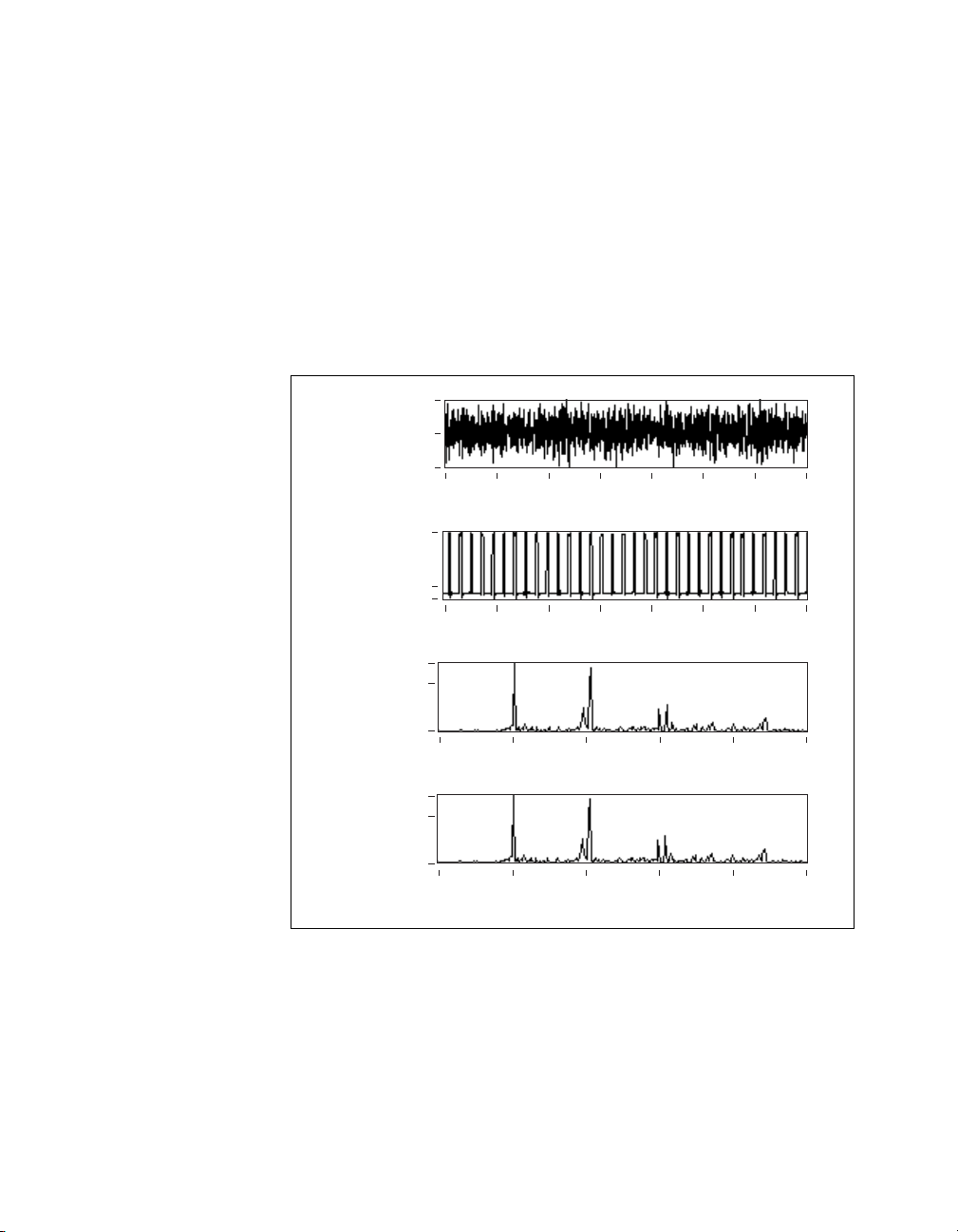You can implement the CIC filter using only addition and subtraction operations, which makes the CIC filter very efficient for online processing. Figure 4-2 shows the power spectrum of the original time sequence and the CIC interpolation filter with an interpolation factor of eight.

Chapter 4 Resampling-Based Order Analysis

Figure 4-2. Original Time Sequence and CIC Interpolation Filter with

an Interpolation Factor of Eight

Resampling Vibration Data

The resampling operation converts a vibration signal from the time domain into the angle domain. To resample vibration data into even angle spaced samples, you must be able to calculate the value of the vibration signal at any time instance.

According to the Nyquist sampling theorem, you can exactly reconstruct the signal for all time instances using band-limited interpolation if and only if the original signal is band limited to half of the sampling rate.

For example, a continuous time signal x(t) that is band limited to f sampled at a sampling rate of f

samples/second yields a discrete sample

given by the following equation.

= x(nTs),

where T

LabVIEW Order Analysis Toolset User Manual 4-4 ni.com

= 1/fs and is the sampling time interval.

/2 Hz and

Chapter 4 Resampling-Based Order Analysis

According to the Nyquist sampling theorem, you can exactly reconstruct the time signal x(t) from samples x(nT

) with the following equation.

π f

(4-1)

t()sin

where h

xˆt() xnT

is a sinc function defined by .

∑

Figure 4-3 shows the plot of h

Figure 4-3. hs(t) with fs = 1

()hsnTst–()

t() sinc fst()

(t) with fs = 1.

----------------------==

You can resample the signal at the equal angle interval time instance by evaluating Equation 4-1 at the desired time. Before resampling, you might need a lowpass anti-aliasing filter if the new sampling rate is lower that the previous sampling rate.

The LabVIEW Order Analysis Toolset uses a digital adaptive-interpolation filter to complete the entire resample process. The bandwidth of the adaptive-interpolation filter automatically changes according to the new sampling rate to prevent the aliasing phenomenon. The stopband attenuation of the interpolation filter controls the accuracy of the resampling. As the stopband attenuation becomes higher, the accuracy of the resampled signal improves.

Slow Roll Compensation

In machine condition monitoring applications, engineers often use a proximity probe to measure the movement of a shaft. The proximity probe can convert the distance between the probe and the shaft into an electrical signal.

Chapter 4 Resampling-Based Order Analysis

When monitoring shaft vibration with a proximity probe, the acquired signal contains not only the vibration of the shaft but also the shaft runout, such as a nonconcentric shaft condition at the probe measurement plane. You can measure the shaft runout at a slow roll speed and can compensate for it in the raw proximity probe signal. Figure 4-4 shows the raw signal acquired from a nonconcentric shaft and the compensated signal.

Rolling Center

Amplitude

Shaft Center

Raw Signal

Amplitude

Compensated Signal

Figure 4-4. Slow Roll Compensation

The LabVIEW Order Analysis Toolset can perform the vector-based slow roll compensation on order magnitudes and phases. The toolset performs slow roll compensation subtracting a slow roll vector from the measured magnitude and phase. Use the OAT Extract Slow Roll Vector VI to compute the slow roll vector from a slow roll signal. Use the OAT Slow Roll Compensation VI to remove the runout components from the measured magnitude and phase. If no slow roll vector is provided, the OAT Slow Roll Compensation VI automatically uses the first magnitude and phase pair as the slow roll vector.

LabVIEW Order Analysis Toolset User Manual 4-6 ni.com

Calculating Rotational Speed

This chapter describes the digital differentiator method used by the LabVIEW Order Analysis Toolset to calculate rotational speed and describes averaging pulses to smooth noisy calculated rotational speed results.

Digital Differentiator Method

To successfully extract order components, create spectral maps, and calculate waveform magnitudes, you need rotational speed as a function of time during the data acquisition process. The LabVIEW Order Analysis Toolset uses a digital differentiator to calculate the rotational speed. The tachometer processing VIs buffer the input tachometer pulses. Because the tachometer-processing VIs buffer the input tachometer pulses, they can use tachometer pulses occurring before and after each time instance when calculating rotational speed. Using tachometer pulses occurring before and after each time instance improves the accuracy of the calculated rotational speed.

Figure 5-1 illustrates a typical tachometer pulse train and the cumulative rotation angle θ of the shaft as a function of time t.

Chapter 5 Calculating Rotational Speed

θ4

θ3

θ2

θ1

t1 t2 t3 t4

(a) Tachometer Pulse

∆θ

t1 t2 t3 t4

(b) Rotation Angle vs. Time

Figure 5-1. Tachometer Signal and Rotation Angle

The arrival time tk of the pulses P(k) in the tachometer signal correspond to the cumulative rotation angle θ(t

θ(t) increases by a fixed angle θ in the time interval between times t t

. As shown in the following equation, you can present rotational speed

k+1

as the first derivative of θ(k).

ϖ3

). The cumulative rotation angle function

and

ω t()

dθ

------=

While the time interval between pulses varies with the rotational speed, the cumulative angle increment remains constant. Calculating the first derivative of θ(t) usually involves step-by-step polynomial curve fitting, which requires multiple computations in each iteration. Instead of observing θ(t) directly, the LabVIEW Order Analysis Toolset observes t(θ), which is the inverse function of θ(t), because calculating the first derivative

LabVIEW Order Analysis Toolset User Manual 5-2 ni.com

Chapter 5 Calculating Rotational Speed

of an equally spaced sequence requires fewer computations than calculating the first derivative of an unequally spaced sequence.

For the evenly separated function series t

, you can use a digital

differentiator to calculate the first derivative. The digital differentiator is implemented as a special FIR filter with the following equation.

-------

≈

∑

∆θ

iM–=

ki–

(5-1)

where h

------

dθ

θθk=

represents the differentiator coefficients.

Rotational speed at each pulse-arrival time instant then is calculated by the following equation.

ω tk()

dθ

------

ttk=

--------------------==

------

dθ

θθk=

The differentiator in Equation 5-1 has an order of 2M. As the order becomes larger, the accuracy of the calculated rotational speed improves. However, as the order becomes larger, the number of pulses needed to calculate the rotational speed also increases. The LabVIEW Order Analysis Toolset can automatically adjust the order of the differentiator according to the number of pulses in the buffer. Automatically adjusting the order of the differentiator improves the accuracy of the calculated rotational speed when the buffer contains a large number of pulses and makes it possible to generate a result even if the buffer contains only two pulses.

Averaging Pulses

Sometimes, the calculated rotational speed is noisy because of error in measuring the arrival time of each pulse. Averaging pulses can smooth noisy calculated rotational speed results. One of the averaging approaches considers two or more pulses as a single pulse by decimating the original

series. Also, the angle increment between two sequential pulses must be

multiplied by the corresponding factor. Because the measurement error of the pulse arrival time is noncumulative, widening the pulse interval decreases the relative error.

Chapter 5 Calculating Rotational Speed

Figure 5-2 shows an example of the rotational speed calculated from the tachometer pulses.

3059.3

3055.0

3050.0

3045.0

Rotational Speed (RPM)

3040.0

Speed (No Average)

19.2 19.3 19.4 19.5 19.6

In Figure 5-2, the dotted line represents the results of calculating the rotational speed with no averaging. The solid line in Figure 5-2 represents the results of calculating the rotational speed averaged by five. As Figure 5-2 shows, the averaged rotational speed is smoother than the non-averaged rotational speed.

Speed (Averaged by 5)

Time (s)

Figure 5-2. Cumulative Revolution and Rotational Speed

LabVIEW Order Analysis Toolset User Manual 5-4 ni.com

Gabor Expansion and Gabor Transform

This appendix presents an overview of the Gabor expansion and the Gabor transform methods used in the LabVIEW Order Analysis Toolset. This appendix also describes application issues associated with using the discrete Gabor-expansion-based time-varying filter.

Gabor Expansion and Gabor Transform Basics

The Gabor expansion characterizes a signal jointly in the time and frequency domains. Although Dennis Gabor introduced the Gabor expansion more than half a century ago, its implementation was an open research topic until Bastiaans discovered the relationship between the Gabor expansion and the short-time Fourier transform (STFT) in the early 1980s.

Over the years, many different implementation schemes for the discrete Gabor expansion were proposed. The LabVIEW Order Analysis Toolset uses an extension of the method originally developed by Wexler and Raz to implement the discrete Gabor expansion. In the method used by the LabVIEW Order Analysis Toolset, lengths of the analysis and synthesis window functions are the same, while perfect reconstruction is guaranteed.

For a discrete sample s[k], the corresponding Gabor expansion is defined by the following equation.

N 1–

sk[] c

where the Gabor coefficients c

∑

n 0=

hk m∆M–[]e

mn,

are computed by a sampled STFT.

m,n

j2 πnk N⁄

(A-1)

Appendix A Gabor Expansion and Gabor Transform

The sampled STFT is also known as the Gabor transform and is represented by the following equation.

N 1–

s˜k[]γ∗km∆M–[]e

mn,

∑

n 0=

j2 πnk– N⁄

(A-2)

where ∆M represents the time sampling interval and N represents the total number of frequency bins.

The ratio between N and ∆M determines the Gabor sampling rate. For numerical stability, the Gabor sampling rate must be greater than or equal to one. Critical sampling occurs when N = ∆M. In critical sampling, the number of Gabor coefficients c

equals the number of original data

m,n

samples s[k]. Over sampling occurs when N/∆M > 1. For over sampling, the number of Gabor coefficients is more than the number of original data samples. In over sampling, the Gabor transform in Equation A-2 contains redundancy, from a mathematical point of view. However, the redundancy in Equation A-2 provides freedom for the selection of better window functions, h[k] and γ[k].

Notice that the positions of the window functions h[k] and γ[k] are interchangeable. In other words, you can use either of the window functions as the synthesis or analysis window function. Therefore, h[k] and γ[k] are usually referred to as dual functions.

The method of the discrete Gabor expansion developed in this appendix requires in Equation A-2 to be a periodic sequence, as shown by the

s˜k[]

following equation.



s˜kiL

+[]

where L of the sequence L to L

represents the length of the signal s[k] and L0 represents the period

s˜k[].

. L0 must be evenly divided by the time sampling interval ∆M. For a

is the smallest integer that is greater than or equal

sk[] 0 kL



0 L



<≤

(A-3)

given window h[k] that always has unit energy, you can compute the

LabVIEW Order Analysis Toolset User Manual A-2 ni.com

Appendix A Gabor Expansion and Gabor Transform

corresponding dual window function from ∆M independent linear systems with the following equation.

--------- 1–

∆M

a˜kp∆MqN++[]γ

∑

p 0=

∗

kp∆M+[]

δ q[]

-----------= 0 k ∆M<≤

(A-4)

where L denotes the window length. denotes a periodic auxiliary function

given by the following equation.



a˜ki2LN–()+[]

hk[] 0 kL<≤

= 0 q



0 Lk2LN–<≤



a˜k[]

------ 1–<≤

Notice that the solution of Equation A-4 is not unique for over sampling. A particularly interesting solution for Equation A-4 is the least mean square error (LMSE). For the LMSE solution, the Euclidean distance between the dual functions is minimum, as given by the following equation.

Aγ u=

----- h–

min

where denotes the matrix form of Equation A-4. When ,

Aγµ= γ h≈

the error is small, and Equation A-2 becomes

≈

∑

k[]hk mT–[]e

mn,

j2 πnk– N⁄

(A-5)

Equations A-5 and A-1 form an orthogonal-like Gabor transform pair. In the case of an orthogonal-like Gabor transform pair, the Gabor coefficients

are the projection of the signal on the synthesis window function h[k].

m, n

If the window length is equal to the signal length, the periodic auxiliary function is simply

a˜kiL+[]hk[]= 0 q

----

<≤

a˜k[]

Appendix A Gabor Expansion and Gabor Transform

Discrete Gabor-Expansion-Based Time-Varying Filter

Initially, discrete Gabor expansion seems to provide a feasible method for converting an arbitrary signal from the time domain into the joint time-frequency domain or vice versa. However, discrete Gabor expansion is effective for converting an arbitrary signal from the time domain into the joint time-frequency domain or vice versa only in the case of critical sampling, ∆M = N. For over sampling, which is the case for most applications, the Gabor coefficients are the subspace of two-dimensional functions. In other words, for an arbitrary two-dimensional function, a corresponding time waveform might not exist. For example, the following equation represents a modified two-dimensional function.

where Φ

denotes a binary mask function whose elements are either

m, n

mn,

mn,cmn,

0 or 1. Applying the Gabor expansion to the modified two-dimensional function results in the following equation.

N 1–

sˆk[] c

∑

n 0=

hk mT–[]e

mn,

j2 πnk N⁄

The following inequality results from Gabor expansion.

k[]γkmT–[]e

∑

j2 πnk– N⁄

The Gabor coefficients of the reconstructed time waveform are not equal to the selected Gabor coefficients .

mn,

≠

mn,

k[]

To overcome the problem of the reconstructed time waveform not equaling the selected Gabor coefficients, use an iterative process. Complete the following steps to perform the iterative process.

1. Determine a binary mask matrix for a set of two-dimensional Gabor coefficients.

2. Apply the mask to the two-dimensional Gabor coefficients to preserve desirable coefficients and remove unwanted coefficients.

3. Compute the Gabor expansion.

LabVIEW Order Analysis Toolset User Manual A-4 ni.com

Appendix A Gabor Expansion and Gabor Transform

4. Compute the new Gabor coefficients after you obtain the time waveform.

5. Repeat steps 1 through 4 until the time waveforms converge.

Without a loss of generality, rewrite the Gabor expansion from Equation A-1 and the Gabor transform from Equation A-2 in matrix form, as shown in the following equations.

CGs=

Gs=

where H denotes the analysis matrix and G denotes the synthesis matrix. Notice that for over sampling, the following relationships are true.

HTGI= GHTI≠

Therefore, in the case of over sampling, the iterative process is described by the following equations.

ΦC=

HTC

C2Gs1GHTΦC==

C3Gs2GHTΦGHTΦCGHTΦ()

ΦC

HTC

C== =

…

GHTΦ()

k 1–

Appendix A Gabor Expansion and Gabor Transform

Ck and converge. with . For with

, the support of C

k ∞→

CkΦC

= k ∞→ CkΦC

in the time-frequency domain is inside the

masked area if and only if the following equation is true.

---- 1–

∗

iN k+[]hiN k m∆M++[] =

∑

i 0=

for 0 ≤ k < N and 0 ≤ m < . Two trivial cases for Equation A-6 are

---- 1–

∑

i 0=

∗

iN k+[]γiN k m∆M++[]

---------

∆M

(A-6)

critical sampling and when γ[k]=h[k].

In critical sampling, N = ∆M. Notice that in the case of critical sampling, the analysis and synthesis windows cannot both be localized in the joint time-frequency domain.

In the case of γ[k]=h[k], the Gabor coefficients C

, after the first iteration,

are the closest in terms of the LMSE to the masked Gabor coefficients ΦC. The masked Gabor coefficients are the desirable Gabor coefficients. The case of γ[k]=h[k] usually implies considerable over sampling, which results in a huge amount of redundancy. The amount of redundancy causes slow computation speed and huge memory consumption, making γ[k]=h[k] an impractical Gabor transform method.

Usually, the LabVIEW Order Analysis Toolset uses the orthogonal-like representation introduced at the end of the Gabor Expansion and Gabor

Transform Basics section. For commonly used window functions, such as

the Gaussian and Hanning windows, the difference between the analysis and synthesis windows is negligible when the over sampling rate is four.

LabVIEW Order Analysis Toolset User Manual A-6 ni.com

References

This appendix lists the reference material used for the LabVIEW Order Analysis Toolset.

• Albright, Michael, and Shie Qian. Comparison of the New Proposed Gabor Order Tracking Technique vs. Other Order Tracking Methods. SAE Noise and Vibration Conference and Exposition. Traverse City, MI, April 30 through May 3, 2001.

• Gade, S., H. Herlufsen, H. Konstantin-Hansen, and H. Vold. Characteristics of the Vold-Kalman Order Tracking Filter. Brüel & Kjær Sound & Vibration Measurement A/S, 1999.

• Hewlett Packard Application Note 243-1. Effective Machinery Measurements using Dynamic Signal Analyzers.

• Qian, Shie, and Dapang Chen. Joint Time-Frequency Analysis. Upper Saddle River, NJ: Prentice Hall PTR, 1996.

Technical Support and Professional Services

Visit the following sections of the National Instruments Web site at

ni.com for technical support and professional services:

• Support—Online technical support resources include the following:

– Self-Help Resources—For immediate answers and solutions,

visit our extensive library of technical support resources available in English, Japanese, and Spanish at resources are available for most products at no cost to registered users and include software drivers and updates, a KnowledgeBase, product manuals, step-by-step troubleshooting wizards, conformity documentation, example code, tutorials and application notes, instrument drivers, discussion forums, a measurement glossary, and so on.

– Assisted Support Options—Contact NI engineers and other

measurement and automation professionals by visiting

ni.com/support. Our online system helps you define your

question and connects you to the experts by phone, discussion forum, or email.

• Training—Visit and interactive CDs. You also can register for instructor-led, hands-on courses at locations around the world.

• System Integration—If you have time constraints, limited in-house technical resources, or other project challenges, NI Alliance Program members can help. To learn more, call your local NI office or visit

ni.com/alliance.

ni.com/training for self-paced tutorials, videos,

ni.com/support. These

If you searched your local office or NI corporate headquarters. Phone numbers for our worldwide offices are listed at the front of this manual. You also can visit the Worldwide Offices section of office Web sites, which provide up-to-date contact information, support phone numbers, email addresses, and current events.

ni.com and could not find the answers you need, contact

ni.com/niglobal to access the branch

Glossary

Numbers/Symbols

∞

2D Two-dimensional.

Infinity.

adaptive filter A type of filter that operates on a recursive algorithm to achieve the goal of

optimum. It is self-designing and suitable for tracking time variations of the input signal, but complete knowledge of the relevant signal characteristics is not available.

aliasing A phenomenon in which an analog signal of a frequency greater than half

the sampling frequency, or Nyquist frequency, appears after sampling at a frequency less than half the sampling frequency. See also anti-aliasing filter and Nyquist frequency.

anti-aliasing filter Analog lowpass filters used before analog-to-digital conversion to filter out

the frequencies greater than half the sampling frequency. See also aliasing and Nyquist frequency.

critical sampling Occurs in Gabor transform when the window length equals the window

shift step. In critical sampling, the number of Gabor coefficients c the number of original data samples s[k].

m, n

equals

dB Decibel.

dual functions Pair of window functions for Gabor transform and Gabor expansion. The

two dual functions are interchangeable. That is, you can use either of the dual functions for a Gabor transform while using the other dual function for a Gabor expansion.

Glossary

FFT Fast Fourier transform.

fundamental component Portion of a signal whose frequency is at the fundamental frequency.

Gabor coefficient The result of Gabor transform.

Gabor expansion The inverse Gabor transform used on Gabor coefficients to recover a time

domain input signal.

Gabor transform One of the invertible joint time-frequency transforms.

harmonic Frequencies that are integer or fractional multiples of a fundamental

frequency.

LMSE Least mean square error.

Nyquist frequency Half the sampling frequency. Any analog frequency component above

the Nyquist frequency will, after sampling, be converted, or aliased, to a frequency below the Nyquist frequency. See also aliasing and anti-aliasing

filter.

order A harmonic related to the rotational speed of a machine.

order analysis The analysis of harmonics related to rotational speed. The application of

harmonic analysis to rotating machinery

LabVIEW Order Analysis Toolset User Manual G-2 ni.com

Glossary

order curves The high power density curves in a spectral map which indicate order

components.

orthogonal-like Gabor transform pair

over sampling Occurs in a Gabor transform when the window length is greater than the

The pair is composed of a Gabor transform and a Gabor expansion when the Gabor coefficients c signal on the synthesis window function h[k].

window shift step. In over sampling, the number of Gabor coefficients c is more than the number of original data samples s[k].

found by each method are the projection of the

m, n

resampling A method to sample a time sequence at a different time interval.

RMS Root mean square.

RPM Revolutions per minute.

STFT Short time Fourier transform.

window shift step The shortest time interval between two windows. In the LabVIEW Order

Analysis Toolset, it is always equal to a quarter (0.25) of the window length. For example, if the window length is 2,048, the window shift is 512.

Index

adaptive filter, 2-15 analysis of rotating machinery, using the

toolset, 1-2

applying an iteration to reconstruct a time

waveform, A-4

calculating rotational speed, 5-1

averaging pulses, 5-3

digital differentiator, 5-1 calculating waveform magnitude, 3-10 contacting National Instruments, C-1 conventions used in the manual, vii critical sampling, definition of, A-2 customer

education, C-1

professional services, C-1

technical support, C-1

DAQ. See data acquisition data acquisition

examples, 1-4

guidelines for, 1-4 diagnostic resources, C-1 displaying spectral maps, 3-8 documentation

conventions used in the manual, vii

getting started, vii

how to use this manual, vii

online library, C-1

National Instruments Order Analysis Toolset User Manual

Specifications and Main Features

Frequently Asked Questions

User Manual

LabVIEW Order Analysis Toolset User Manual

Support

Worldwide Technical Support and Product Information

National Instruments Corporate Headquarters

Worldwide Offices

Important Information

Warranty

Copyright

Trademarks

Patents

WARNING REGARDING USE OF NATIONAL INSTRUMENTS PRODUCTS

Contents

About This Manual

How to Use This Manual

Conventions

Related Documentation

Overview of the LabVIEW Order Analysis Toolset

Overview of the LabVIEW Order Analysis Start-Up Kit

Important Considerations for the Analysis of Rotating Machinery

System Requirements

Installation

Example VIs

Acquiring Data for Example VIs

Configuring DAQ Hardware Used with Examples

Acquire Data (Analog Tach) VI

Figure 1-1. Acquire Data (Analog Tach) VI Configuration Tab

Figure 1-2. Acquire Data (Analog Tach) VI Acquisition Tab

Acquire Data with PXI 4472 and TIO VI

Figure 1-3. Acquire Data with PXI 4472 and TIO VI Configuration Tab

Figure 1-4. Acquire Data with PXI 4472 and TIO VI Acquisition Tab

Order Analysis Definition and Application

Order Analysis Basics

Figure 2-1. Order and Frequency Domain Display of a Shaft Rotating at 3,000 rpm

Figure 2-2. Order Spectrum of a PC Fan with Seven Blades and Four Coils

Effect of Rotational Speed on Order Identification

Constant Rotational Speed

Figure 2-3. PC Fan Running at Constant Speed

Variable Rotational Speed

Figure 2-4. Constant Frequency

Figure 2-5. Frequency Changes Over Time

Figure 2-6. Fan Run-Up

Harmonic Analysis

Order Analysis

Order Analysis Methods

Gabor Transform

Figure 2-7. Padding Schemes

Figure 2-8. Padding Examples

Resampling

Figure 2-9. Resampling

Figure 2-10. Spectrum of Angle Samples

Adaptive Filter

Overview of Gabor Order Analysis

Figure 3-1. Frequency-Time Spectral Map of a Vibration Signal

Figure 3-2. Gabor Order Analysis Diagram

Extracting the Order Components

Figure 3-3. Constant Frequency Bandwidth and Constant Order Bandwidth

Masking

Extracting Orders

Figure 3-4. Gabor Coefficients

Reconstructing the Signal

Figure 3-5. Original Signal and Extracted Order Component

Figure 3-6. Spectrum of Reconstructed Signal

Displaying Spectral Maps

Figure 3-7. 2D Spectral Maps

Calculating Waveform Magnitude

LabVIEW Order Analysis Toolset Resampling Method

Figure 4-1. Resampling-Based Order Analysis Diagram

Determining the Time Instance for Resampling

Resampling Vibration Data

Figure 4-3. hs(t) with fs = 1

Slow Roll Compensation

Figure 4-4. Slow Roll Compensation

Digital Differentiator Method

Figure 5-1. Tachometer Signal and Rotation Angle

Averaging Pulses

Figure 5-2. Cumulative Revolution and Rotational Speed