

Page 1

Motion Control
NI-MotionTM User Manual
NI-Motion User Manual
November 2005
371242B-01
Page 2

support
Worldwide Technical Support and Product Information
ni.com
National Instruments Corporate Headquarters
11500 North Mopac Expressway Austin, Texas 78759-3504 USA Tel: 512 683 0100
Worldwide Offices
Australia 1800 300 800, Austria 43 0 662 45 79 90 0, Belgium 32 0 2 757 00 20, Brazil 55 11 3262 3599,
Canada 800 433 3488, China 86 21 6555 7838, Czech Republic 420 224 235 774, Denmark 45 45 76 26 00,
Finland 385 0 9 725 725 11, France 33 0 1 48 14 24 24, Germany 49 0 89 741 31 30, India 91 80 51190000,
Israel 972 0 3 6393737, Italy 39 02 413091, Japan 81 3 5472 2970, Korea 82 02 3451 3400,
Lebanon 961 0 1 33 28 28, Malaysia 1800 887710, Mexico 01 800 010 0793, Netherlands 31 0 348 433 466,
New Zealand 0800 553 322, Norway 47 0 66 90 76 60, Poland 48 22 3390150, Portugal 351 210 311 210,
Russia 7 095 783 68 51, Singapore 1800 226 5886, Slovenia 386 3 425 4200, South Africa 27 0 11 805 8197,
Spain 34 91 640 0085, Sweden 46 0 8 587 895 00, Switzerland 41 56 200 51 51, Taiwan 886 02 2377 2222,
Thailand 662 278 6777, United Kingdom 44 0 1635 523545
For further support information, refer to the Technical Support and Professional Services appendix. To comment
on National Instruments documentation, refer to the National Instruments Web site at ni.com/info and enter
the info code feedback.
© 2003–2005 National Instruments Corporation. All rights reserved.
Page 3

Important Information
Warranty
The media on which you receive National Instruments software are warranted not to fail to execute programming instructions, due to defects
in materials and workmanship, for a period of 90 days from date of shipment, as evidenced by receipts or other documentation. National
Instruments will, at its option, repair or replace software media that do not execute programming instructions if National Instruments receives
notice of such defects during the warranty period. National Instruments does not warrant that the operation of the software shall be
uninterrupted or error free.
A Return Material Authorization (RMA) number must be obtained from the factory and clearly marked on the outside of the package before
any equipment will be accepted for warranty work. National Instruments will pay the shipping costs of returning to the owner parts which are
covered by warranty.
National Instruments believes that the information in this document is accurate. The document has been carefully reviewed for technical
accuracy. In the event that technical or typographical errors exist, National Instruments reserves the right to make changes to subsequent
editions of this document without prior notice to holders of this edition. The reader should consult National Instruments if errors are suspected.
In no event shall National Instruments be liable for any damages arising out of or related to this document or the information contained in it.
E
XCEPT AS SPECIFIED HEREIN, NATIONAL INSTRUMENTS MAKES NO WARRANTIES, EXPRESS OR IMPLIED, AND SPECIFICALLY DISCLAIMS ANY WAR RANTY OF
MERCHANTABILITY OR FITNESS FOR A PARTICULAR PURPOSE . CUSTOMER’S RIGHT TO RECOVER DAMAGES CAUSED BY FAULT OR NEGLIGENCE ON THE PART OF
N
ATIONAL INSTRUMENTS SHALL BE LIMITED TO THE AMOUNT THERETOFORE PAID BY THE CUSTOMER. NATIONAL INSTRUMENTS WILL NOT BE LIABLE FOR
DAMAGES RESULTING FROM LOSS OF DATA, PROFITS, USE OF PRODUCTS, OR INCIDENTAL OR CONSEQUENTIAL DAMAGES, EVEN IF ADVISED OF THE POSS IBILITY
THEREOF. This limitation of the liability of National Instruments will apply regardless of the form of action, whether in contract or tort, including
negligence. Any action against National Instruments must be brought within one year after the cause of action accrues. National Instruments
shall not be liable for any delay in performance due to causes beyond its reasonable control. The warranty provided herein does not cover
damages, defects, malfunctions, or service failures caused by owner’s failure to follow the National Instruments installation, operation, or
maintenance instructions; owner’s modification of the product; owner’s abuse, misuse, or negligent acts; and power failure or surges, fire,
flood, accident, actions of third parties, or other events outside reasonable control.
Copyright
Under the copyright laws, this publication may not be reproduced or transmitted in any form, electronic or mechanical, including photocopying,
recording, storing in an information retrieval system, or translating, in whole or in part, without the prior written consent of National
Instruments Corporation.
Trademarks
National Instruments, NI, ni.com, and LabVIEW are trademarks of National Instruments Corporation. Refer to the Terms of Use section
on
ni.com/legal for more information about National Instruments trademarks.
®
is the registered trademark of Apple Computer, Inc. Other product and company names mentioned herein are trademarks or trade
FireWire
names of their respective companies.
Patents
For patents covering National Instruments products, refer to the appropriate location: Help»Patents in your software, the patents.txt file
on your CD, or ni.com/patents.
WARNING REGARDING USE OF NATIONAL INSTRUMENTS PRODUCTS
(1) NATIONAL INSTRUMENTS PRODUCTS ARE NOT DESIGNED WITH COMPONENTS AND TESTING FOR A LEVEL OF
RELIABILITY SUITABLE FOR USE IN OR IN CONNECTION WITH SURGICAL IMPLANTS OR AS CRITICAL COMPONENTS IN
ANY LIFE SUPPORT SYSTEMS WHOSE FAILURE TO PERFORM CAN REASONABLY BE EXPECTED TO CAUSE SIGNIFICANT
INJURY TO A HUMAN.
(2) IN ANY APPLICATION, INCLUDING THE ABOVE, RELIABILITY OF OPERATION OF THE SOFTWARE PRODUCTS CAN BE
IMPAIRED BY ADVERSE FACTORS, INCLUDING BUT NOT LIMITED TO FLUCTUATIONS IN ELECTRICAL POWER SUPPLY,
COMPUTER HARDWARE MALFUNCTIONS, COMPUTER OPERATING SYSTEM SOFTWARE FITNESS, FITNESS OF COMPILERS
AND DEVELOPMENT SOFTWARE USED TO DEVELOP AN APPLICATION, INSTALLATION ERRORS, SOFTWARE AND
HARDWARE COMPATIBILITY PROBLEMS, MALFUNCTIONS OR FAILURES OF ELECTRONIC MONITORING OR CONTROL
DEVICES, TRANSIENT FAILURES OF ELECTRONIC SYSTEMS (HARDWARE AND/OR SOFTWARE), UNANTICIPATED USES OR
MISUSES, OR ERRORS ON THE PART OF THE USER OR APPLICATIONS DESIGNER (ADVERSE FACTORS SUCH AS THESE ARE
HEREAFTER COLLECTIVELY TERMED “SYSTEM FAILURES”). ANY APPLICATION WHERE A SYSTEM FAILURE WOULD
CREATE A RISK OF HARM TO PROPERTY OR PERSONS (INCLUDING THE RISK OF BODILY INJURY AND DEATH) SHOULD
NOT BE RELIANT SOLELY UPON ONE FORM OF ELECTRONIC SYSTEM DUE TO THE RISK OF SYSTEM FAILURE. TO AVOID
DAMAGE, INJURY, OR DEATH, THE USER OR APPLICATION DESIGNER MUST TAKE REASONABLY PRUDENT STEPS TO
PROTECT AGAINST SYSTEM FAILURES, INCLUDING BUT NOT LIMITED TO BACK-UP OR SHUT DOWN MECHANISMS.
BECAUSE EACH END-USER SYSTEM IS CUSTOMIZED AND DIFFERS FROM NATIONAL INSTRUMENTS' TESTING
PLATFORMS AND BECAUSE A USER OR APPLICATION DESIGNER MAY USE NATIONAL INSTRUMENTS PRODUCTS IN
COMBINATION WITH OTHER PRODUCTS IN A MANNER NOT EVALUATED OR CONTEMPLATED BY NATIONAL
INSTRUMENTS, THE USER OR APPLICATION DESIGNER IS ULTIMATELY RESPONSIBLE FOR VERIFYING AND VALIDATING
THE SUITABILITY OF NATIONAL INSTRUMENTS PRODUCTS WHENEVER NATIONAL INSTRUMENTS PRODUCTS ARE
INCORPORATED IN A SYSTEM OR APPLICATION, INCLUDING, WITHOUT LIMITATION, THE APPROPRIATE DESIGN,
PROCESS AND SAFETY LEVEL OF SUCH SYSTEM OR APPLICATION.
Page 4

Contents
About This Manual
Conventions ...................................................................................................................xiii
Documentation and Examples .......................................................................................xiv
Chapter 1
Introduction to NI-Motion
About NI-Motion ...........................................................................................................1-1
NI-Motion Architecture .................................................................................................1-1
Software and Hardware Interaction.................................................................1-2
NI Motion Controller Architecture..................................................................1-2
NI 73xx Architecture.........................................................................1-2
NI Motion Controller Functional Architecture................................................1-4
NI SoftMotion Controller Architecture.............................................1-7
NI SoftMotion Controller Communication Watchdog ..................................................1-9
PART I
Introduction
Chapter 2
Creating NI-Motion Applications
Creating a Generic NI-Motion Application ...................................................................2-1
Adding Measurements to an NI-Motion Application ....................................................2-2
PART II
Configuring Motion Control
Chapter 3
Tuning Servo Systems
NI SoftMotion Controller Considerations .....................................................................3-1
NI SoftMotion Controller for CANopen .........................................................3-1
NI SoftMotion Controller for Ormec ..............................................................3-1
Using Control Loops to Tune Servo Motors .................................................................3-1
Control Loop ...................................................................................................3-2
PID Loop Descriptions......................................................................3-4
Velocity Feedback ...........................................................................................3-9
NI Motion Controllers with Velocity Amplifiers............................................3-10
© National Instruments Corporation v NI-Motion User Manual
Page 5

Contents
PART III
Programming with NI-Motion
Chapter 4
What You Need to Know about Moves
Move Profiles ................................................................................................................ 4-1
Trapezoidal...................................................................................................... 4-1
S-Curve ........................................................................................................... 4-2
Basic Moves ..................................................................................... 4-2
Coordinate Space.............................................................................. 4-3
Multi-Starts versus Coordinate Spaces............................................. 4-3
Trajectory Parameters ..................................................................................... 4-4
NI 73xx Floating-Point versus Fixed-Point ...................................... 4-4
NI 73xx Time Base ........................................................................... 4-5
NI 73xx Arc Move Limitations ....................................................................... 4-13
Timing Loops ................................................................................................................ 4-14
Status Display ................................................................................................. 4-14
Graphing Data ................................................................................................. 4-14
Event Polling................................................................................................... 4-14
Chapter 5
Straight-Line Moves
Position-Based Straight-Line Moves............................................................................. 5-1
Straight-Line Move Algorithm ....................................................................... 5-1
C/C++ Code ....................................................................................................5-5
1D Straight-Line Move Code ........................................................... 5-5
2D Straight-Line Move Code ........................................................... 5-7
Velocity-Based Straight-Line Moves ............................................................................ 5-10
Algorithm ........................................................................................................ 5-11
LabVIEW Code............................................................................................... 5-13
C/C++ Code ....................................................................................................5-13
Velocity Profiling Using Velocity Override.................................................................. 5-17
Algorithm ........................................................................................................ 5-18
LabVIEW Code............................................................................................... 5-19
C/C++ Code ....................................................................................................5-20
NI-Motion User Manual vi ni.com
Page 6

Chapter 6
Arc Moves
Circular Arcs..................................................................................................................6-1
Arc Move Algorithm .......................................................................................6-3
LabVIEW Code ...............................................................................................6-4
C/C++ Code.....................................................................................................6-4
Spherical Arcs................................................................................................................6-7
Algorithm ........................................................................................................6-9
LabVIEW Code ...............................................................................................6-10
C/C++ Code.....................................................................................................6-10
Helical Arcs ...................................................................................................................6-13
Algorithm ........................................................................................................6-14
LabVIEW Code ...............................................................................................6-15
C/C++ Code.....................................................................................................6-15
Chapter 7
Contoured Moves
Overview........................................................................................................................7-1
Arbitrary Contoured Moves...........................................................................................7-2
Contoured Move Algorithm ............................................................................7-3
LabVIEW Code ...............................................................................................7-5
C/C++ Code.....................................................................................................7-6
Contents
Absolute versus Relative Contouring ...............................................7-4
Chapter 8
Reference Moves
Find Reference Move.....................................................................................................8-1
Reference Move Algorithm.............................................................................8-2
LabVIEW Code ...............................................................................................8-3
C/C++ Code.....................................................................................................8-3
Chapter 9
Blending Moves
Blending.........................................................................................................................9-1
Superimpose Two Moves ................................................................................9-2
Blend after First Move Is Complete ................................................................9-3
Blend after Delay.............................................................................................9-4
Blending Algorithm.........................................................................................9-5
LabVIEW Code ...............................................................................................9-6
C/C++ Code.....................................................................................................9-7
© National Instruments Corporation vii NI-Motion User Manual
Page 7

Contents
Chapter 10
Electronic Gearing and Camming
Gearing .......................................................................................................................... 10-1
Algorithm ........................................................................................................ 10-2
Gear Master ...................................................................................... 10-4
LabVIEW Code............................................................................................... 10-5
C/C++ Code ....................................................................................................10-5
Camming ....................................................................................................................... 10-8
Algorithm ........................................................................................................ 10-11
Camming Table............................................................................................... 10-12
Slave Offset ...................................................................................... 10-15
Master Offset .................................................................................... 10-17
LabVIEW Code............................................................................................... 10-19
C/C++ Code ....................................................................................................10-19
Chapter 11
Acquiring Time-Sampled Position and Velocity Data
Algorithm ......................................................................................................................11-2
LabVIEW Code ............................................................................................................. 11-4
C/C++ Code................................................................................................................... 11-4
Chapter 12
Synchronization
Absolute Breakpoints .................................................................................................... 12-2
Buffered Breakpoints (NI 7350 only) ............................................................. 12-3
Buffered Breakpoint Algorithm........................................................ 12-4
LabVIEW Code ................................................................................12-5
C/C++ Code...................................................................................... 12-5
Single Position Breakpoints ............................................................................ 12-8
Single Position Breakpoint Algorithm ............................................. 12-8
LabVIEW Code ................................................................................12-9
C/C++ Code...................................................................................... 12-10
Relative Position Breakpoints ....................................................................................... 12-12
Relative Position Breakpoints Algorithm ....................................................... 12-13
LabVIEW Code............................................................................................... 12-14
C/C++ Code ....................................................................................................12-14
Periodically Occurring Breakpoints .............................................................................. 12-16
Periodic Breakpoints (NI 7350 only) .............................................................. 12-17
Periodic Breakpoint Algorithm ........................................................ 12-17
LabVIEW Code ................................................................................12-18
C/C++ Code...................................................................................... 12-18
NI-Motion User Manual viii ni.com
Page 8

Modulo Breakpoints (NI 7330, NI 7340 and NI 7390 only) .........................................12-21
Modulo Breakpoints Algorithm ......................................................................12-23
LabVIEW Code ...............................................................................................12-24
C/C++ Code.....................................................................................................12-25
High-Speed Capture.......................................................................................................12-27
Buffered High-Speed Capture (NI 7350 only) ................................................12-27
Buffered High-Speed Capture Algorithm .......................................................12-28
LabVIEW Code ...............................................................................................12-29
C/C++ Code.....................................................................................................12-29
Non-Buffered High-Speed Capture.................................................................12-32
High-Speed Capture Algorithm.......................................................................12-33
LabVIEW Code ...............................................................................................12-34
C/C++ Code.....................................................................................................12-35
Real-Time System Integration Bus (RTSI) ...................................................................12-37
RTSI Implementation on the Motion Controller .............................................12-38
Position Breakpoints Using RTSI ...................................................................12-39
Encoder Pulses Using RTSI ............................................................................12-39
Software Trigger Using RTSI .........................................................................12-39
High-Speed Capture Input Using RTSI...........................................................12-40
Chapter 13
Torque Control
Analog Feedback ...........................................................................................................13-1
Torque Control Using Analog Feedback Algorithm .......................................13-3
LabVIEW Code ...............................................................................................13-4
C/C++ Code.....................................................................................................13-5
Monitoring Force ...........................................................................................................13-8
Torque Control Using Monitoring Force Algorithm.......................................13-9
LabVIEW Code ...............................................................................................13-10
C/C++ Code.....................................................................................................13-11
Speed Control Based on Analog Value .........................................................................13-14
Speed Control Based on Analog Feedback Algorithm....................................13-14
LabVIEW Code ...............................................................................................13-15
C/C++ Code.....................................................................................................13-16
Contents
Chapter 14
Onboard Programs
Using Onboard Programs with the NI SoftMotion Controller ......................................14-1
Using Onboard Programs with NI 73xx Motion Controllers .........................................14-2
Writing Onboard Programs .............................................................................14-3
Algorithm ........................................................................................................14-4
LabVIEW Code ...............................................................................................14-5
© National Instruments Corporation ix NI-Motion User Manual
Page 9

Contents
C/C++ Code ....................................................................................................14-6
Running, Stopping, and Pausing Onboard Programs .................................................... 14-8
Running an Onboard Program ........................................................................ 14-8
Stopping an Onboard Program........................................................................ 14-8
Pausing/Resuming an Onboard Program ........................................................ 14-8
Automatic Pausing............................................................................ 14-9
Single-Stepping Using Pause............................................................ 14-9
Conditionally Executing Onboard Programs................................................................. 14-9
Onboard Program Conditional Execution Algorithm ..................................... 14-11
LabVIEW Code............................................................................................... 14-12
C/C++ Code ....................................................................................................14-12
Using Onboard Memory and Data ................................................................................14-14
Algorithm ........................................................................................................ 14-15
LabVIEW Code............................................................................................... 14-16
C/C++ Code ....................................................................................................14-17
Branching Onboard Programs ....................................................................................... 14-19
Onboard Program Algorithm .......................................................................... 14-20
LabVIEW Code............................................................................................... 14-21
C/C++ Code ....................................................................................................14-22
Math Operations ............................................................................................................ 14-24
Indirect Variables ..........................................................................................................14-24
Onboard Buffers ............................................................................................................ 14-25
Algorithm ........................................................................................................ 14-26
Synchronizing Host Applications with Onboard Programs .......................................... 14-26
LabVIEW Code............................................................................................... 14-28
C/C++ Code ....................................................................................................14-30
Onboard Subroutines ..................................................................................................... 14-34
Algorithm ........................................................................................................ 14-34
LabVIEW Code............................................................................................... 14-35
C/C++ Code ....................................................................................................14-38
Automatically Starting Onboard Programs ................................................................... 14-42
Changing a Time Slice .................................................................................................. 14-42
PART IV
Creating Applications Using NI-Motion
Chapter 15
Scanning
Connecting Straight-Line Move Segments ................................................................... 15-1
Raster Scanning Using Straight Lines Algorithm...........................................15-2
LabVIEW Code............................................................................................... 15-3
C/C++ Code ....................................................................................................15-4
NI-Motion User Manual x ni.com
Page 10

Blending Straight-Line Move Segments........................................................................15-7
Raster Scanning Using Blended Straight Lines Algorithm.............................15-8
LabVIEW Code ...............................................................................................15-9
C/C++ Code.....................................................................................................15-10
User-Defined Scanning Path..........................................................................................15-13
User-Defined Scanning Path Algorithm..........................................................15-15
LabVIEW Code ...............................................................................................15-16
C/C++ Code.....................................................................................................15-17
Chapter 16
Rotating Knife
Solution..........................................................................................................................16-1
Algorithm ........................................................................................................16-3
LabVIEW Code ...............................................................................................16-4
C/C++ Code.....................................................................................................16-5
Appendix A
Sinusoidal Commutation for Brushless Servo Motion Control
Appendix B
Initializing the Controller Programmatically
Contents
Appendix C
Using the Motion Controller with the LabVIEW Real-Time Module
Appendix D
Technical Support and Professional Services
Glossary
Index
© National Instruments Corporation xi NI-Motion User Manual
Page 11

About This Manual
This manual provides information about the NI-Motion driver software,
including background, configuration, and programming information.
The purpose of this manual is to provide a basic understanding of the
NI-Motion driver software, and provide programming steps and examples
to help you develop NI-Motion applications.
This manual is intended for experienced LabVIEW, C/C++, or other
developers. Code instructions and examples assume a working knowledge
of the given programming language. This manual also assumes a general
knowledge of motion control terminology and development requirements.
This manual pertains to all NI motion controllers that use the NI-Motion
driver software.
Conventions
The following conventions appear in this manual:
<> Angle brackets that contain numbers separated by an ellipsis represent a
range of values associated with a bit or signal name—for example,
AO <3..0>.
[ ] Square brackets enclose optional items—for example, [
» The » symbol leads you through nested menu items and dialog box options
to a final action. The sequence File»Page Setup»Options directs you to
pull down the File menu, select the Page Setup item, and select Options
from the last dialog box.
This icon denotes a tip, which alerts you to advisory information.
This icon denotes a note, which alerts you to important information.
This icon denotes a caution, which advises you of precautions to take to
avoid injury, data loss, or a system crash.
bold Bold text denotes items that you must select or click in the software, such
as menu items and dialog box options. Bold text also denotes parameter
names.
© National Instruments Corporation xiii NI-Motion User Manual
response].
Page 12

About This Manual
italic Italic text denotes variables, emphasis, a cross reference, or an introduction
to a key concept. Italic text also denotes text that is a placeholder for a word
or value that you must supply.
monospace Text in this font denotes text or characters that you should enter from the
keyboard, sections of code, programming examples, and syntax examples.
This font is also used for the proper names of disk drives, paths, directories,
programs, subprograms, subroutines, device names, functions, operations,
variables, filenames, and extensions.
monospace bold Monospace bold text indicates a portion of code with structural
significance.
monospace italic Monospace italic text indicates a portion of code that is commented out.
Documentation and Examples
In addition to this manual, NI-Motion includes the following
documentation to help you create motion applications:
• Getting Started with NI-Motion for NI 73xx Motion Controllers—This
document provides installation instructions and general information
about the NI-Motion product.
• Getting Started: NI SoftMotion Controller for Ormec
ServoWire SM Drives—Refer to this document for information about
getting started with the NI SoftMotion Controller for Ormec.
• Getting Started: NI SoftMotion Controller for Copley CANopen
Drives—Refer to this document for information about getting started
with the NI SoftMotion Controller for CANopen.
• NI-Motion VI Help—Refer to this document for specific information
about NI-Motion LabVIEW VIs.
• NI-Motion Function Help—Refer to this document for specific
information about NI-Motion C/C++ functions.
• Measurement & Automation Explorer Help for Motion—Refer to this
document for configuration information.
• NI-Motion ReadMe—Refer to this HTML document for information
about hardware and software installation and information about
changes to the NI-Motion driver software in the current version. This
document also contains last-minute information about NI-Motion.
• Application notes—For information about advanced NI-Motion
concepts and applications, visit
ni.com/appnotes.nsf/.
NI-Motion User Manual xiv ni.com
Page 13

About This Manual
• NI Developer Zone (NIDZ)—Visit the NI Developer Zone, at
ni.com/zone, for example programs, tutorials, technical
presentations, the Instrument Driver Network, a measurement
glossary, an online magazine, a product advisor, and a community area
where you can share ideas, questions, and source code with motion
developers around the world.
• Motion Hardware Advisor—Visit the National Instruments Motion
Hardware Advisor at
ni.com/devzone/advisors/motion/ to
select motors and stages appropriate to the motion control application.
In addition to the NI Developer Zone, you can find NI-Motion C/C++
and Visual Basic programming examples in the
FlexMotion\Examples
default directory is
NI-Motion
.
folder where you installed NI-Motion. The
Program Files\National Instruments\
NI-Motion\
You can find LabVIEW example programs under
examples\Motion
in the directory where you installed LabVIEW. You can find
LabWindows
™
/CVI™ examples under samples\Motion in the directory
where you installed LabWindows/CVI.
You can find the NI-Motion C/C++ and LabVIEW example code
referenced in this manual in the
Examples\NI-Motion User Manual
NI-Motion\Documentation\
folder where you installed
NI-Motion.
© National Instruments Corporation xv NI-Motion User Manual
Page 14

Introduction
This user manual provides information about the NI-Motion driver
software, motion control setup, and specific task-based instructions for
creating motion control applications using the LabVIEW and C/C++
application development environments.
Part I covers the following topics:
• Introduction to NI-Motion
• Creating NI-Motion Applications
Part I
© National Instruments Corporation I-1 NI-Motion User Manual
Page 15

Introduction to NI-Motion
About NI-Motion
NI-Motion is the driver software for National Instruments 73xx motion
controllers and the NI SoftMotion Controller. You can use NI-Motion to
create motion control applications using the included library of LabVIEW
VIs and C/C++ functions.
National Instruments also offers the Motion Assistant and NI-Motion
development tools for Visual Basic.
NI-Motion Architecture
The NI-Motion driver software architecture is based on the interaction
between the NI motion controllers and a host computer. This interaction
includes the hardware and software interface and the physical and
functional architecture of the NI motion controllers.
1
© National Instruments Corporation 1-1 NI-Motion User Manual
Page 16

Chapter 1 Introduction to NI-Motion
Software and Hardware Interaction
NI Motion Assistant
Graphical Prototyping Tool
Creates ADE
Code
Measurement and
Automation Explorer
Configuration Utility
NI-Motion Driver Software
NI Motion Controller
Figure 1-1. NI Motion Control Hardware and Software Interaction
Note
The last block in Figure 1-1 is not applicable to the NI SoftMotion Controller.
NI Motion Controller Architecture
This section includes information about the architecture for both the 73xx
family of NI motion controllers and the NI SoftMotion Controller.
NI 73xx Architecture
NI 73xx controllers use a dual-processor architecture. The two processors,
a central processing unit (CPU) and a digital signal processor (DSP), form
the backbone of the NI motion controller. The controller plugs into a
variety of slots, including PCI slots, or to a PC using a high-speed serial
interface, such as IEEE 1394 (FireWire
Application Development Environments:
LabVIEW, Visual Basic, and C++
®
).
NI-Motion User Manual 1-2 ni.com
Page 17

Chapter 1 Introduction to NI-Motion
The controller CPU is a 32-bit micro-controller running an embedded real
time, multitasking operating system. This CPU offers the performance and
determinism needed to solve most complex motion applications. The CPU
performs command execution, host synchronization, I/O reaction, and
system supervision.
The DSP has the primary responsibility of fast closed-loop control with
simultaneous position, velocity, and trajectory maintenance on multiple
axes. The DSP also closes the position and velocity loops, and directly
commands the torque to the drive or amplifier.
Motion I/O occurs in hardware on an FPGA and consists of
limit/home switch detection, position breakpoint, and high-speed capture.
This ensures very low latencies in the range of hundreds of nanoseconds
for breakpoints and high-speed captures. Refer to Chapter 12,
Synchronization, for information about breakpoints and high-speed
capture.
The motion controller processor is monitored by a watchdog timer, which
is hardware that can be used to automatically detect software anomalies and
reset the processor if any occur. The watchdog timer checks for proper
processor operation. If the firmware on the motion controller is unable to
process functions within 62 ms, the watchdog timer resets the motion
controller and disallows further communications until you explicitly reset
the motion controller. This ensures the real-time operation of the motion
control system. The following functions may take longer than 62 ms to
process.
• Save Defaults
• Reset Defaults
• Enable Auto Start
• Object Memory Management
• Clear Buffer
• End Storage
These functions are marked as non-real-time functions. Refer to the
NI-Motion Function Help or the NI-Motion VI Help for more information.
© National Instruments Corporation 1-3 NI-Motion User Manual
Page 18

Chapter 1 Introduction to NI-Motion
Figure 1-2 illustrates the physical architecture of the NI motion controller
hardware.
Host Computer
Microprocessor
Running a Real-Time
Operating System
PC
Supervisory/
Communications/
User-defined Onboard
Programs
Watchdog
Timer
Figure 1-2. Physical NI Motion Controller Architecture
Because the NI SoftMotion Controller is not a hardware device, information about
Tip
its architecture is not covered in this section. Refer to the NI SoftMotion Controller
Architecture section for information about the functional architecture that is specific to the
NI SoftMotion Controller.
NI Motion Controller Functional Architecture
Functionally, the architecture of the NI 73xx motion controllers and the
NI SoftMotion Controller is generally divided into four components:
supervisory control, trajectory generator, control loop, and motion I/O. For
the NI SoftMotion Controller, the motion I/O component is separate from
the controller. Refer to Figure 1-3 and Figure 1-4 for an illustration of how
the components of the 73xx and NI SoftMotion Controller interact.
NI Motion Controller
Processor (DSP)
Encoders and Motion I/O
Digital Signal
Control Loop and
Trajectory Generation
FPGAs
NI-Motion User Manual 1-4 ni.com
Page 19

Chapter 1 Introduction to NI-Motion
Figure 1-3 shows the components of the NI 73xx motion controllers.
Typical NI 73xx Motion Controller Architecture
Supervisory Control
Host
Host
Bus
Microcontroller running RTOS/DSPs/FPGAs
Trajectory Generation
Figure 1-3. Typical NI 73xx Motion Controller Functional Architecture
Figure 1-4 shows the components of the NI SoftMotion controller.
NI SoftMotion Controller Architecture
Supervisory Control
Trajectory Generation
Bus
Any CPU on a real-time environment
Software is separate from the I/O
Control Loop
Control Loop
To drive
From
feedback
Analog & Digital I/O
& sensors
To drive
From
feedback
Analog & Digital I/O
& sensors
Figure 1-4. NI SoftMotion Controller Functional Architecture
© National Instruments Corporation 1-5 NI-Motion User Manual
Page 20

Chapter 1 Introduction to NI-Motion
Figure 1-5 illustrates the functional architecture of NI motion controllers.
Supervisory Control
(ms)
User API
Interface
Supervisory
Control
Commands for
Trajectory Generator
Trajectory Generation
(ms)
Cruise
Jerk
Accel
Velocity
Time
dt
Set Point
Jerk
Decel
Interpolation
Control Loop (µs)
(with Interpolation)
PID
Output
Event Monitoring Interface
I/O
New
Set Point
Updated
Updates Trajectory
Generator Based on
I/O And User
Response
Feedback
Sensor
Figure 1-5. NI Motion Controller Functional Architecture
The following list describes how each component of the 73xx controllers
and the NI SoftMotion Controller functions:
• Supervisory control—Performs all the command sequencing and
coordination required to carry out the specified operation
– System initialization, which includes homing to a zero position
– Event handling, which includes electronic gearing, triggering
outputs based on position, updating profiles based on user defined
events, and so on
– Fault Detection, which includes stopping moves on a limit switch
encounter, safe system reaction to emergency stop or drive faults,
watchdog, and so on
• Trajectory generator provides path planning based on the profile
specified by the user
• Control loop—Performs fast, closed-loop control with simultaneous
position, velocity, and trajectory maintenance on one or more axes
NI-Motion User Manual 1-6 ni.com
Page 21

Chapter 1 Introduction to NI-Motion
The control loop handles closing the position/velocity loop based on
feedback, and it defines the response and stability of the system. For
stepper systems, the control loop is replaced with a step generation
component. To enable the control loop to execute faster than the
trajectory generation, an interpolation component, or spline engine, the
control loop interpolates between setpoints calculated by the trajectory
generator. Refer to Figure 1-5 for an illustration of the spline engine.
• Motion I/O—Analog and digital I/O that sends and receives signals
from the rest of the motion control system. Typically, the analog output
is used as a command signal for the drive, and the digital I/O is used
for quadrature encoder signals as feedback from the motor. The motion
I/O performs position breakpoint and high speed capture. Also, the
supervisory control uses the motion I/O to achieve certain required
functionality, such as reacting to limit switches and creating the
movement modes needed to initialize the system.
NI SoftMotion Controller Architecture
The NI-Motion architecture for the NI SoftMotion Controller uses standard
PC-based platforms and open standards to connect intelligent drives to a
real-time host. In this architecture, the software components of the motion
controller run on a real-time host and all I/O is implemented in the drives.
This separation of I/O from the motion controller software components
helps to lower system cost and improve reliability by improving
connectivity. Open standards, such as IEEE 1394 and CANopen, are
used to connect these components.
NI SoftMotion Controller for Ormec
When you use the NI SoftMotion Controller with an Ormec device, you can
daisy chain up to 15 drives together and connect them to the real-time host.
The real-time isochronous mode of the IEEE 1394 bus is used to transfer
data between the drives and the host. Figure 1-6 shows the NI SoftMotion
Controller component architecture that applies when the controller is used
with an Ormec device.
The supervisory control and trajectory generation loops execute every
millisecond. If the control loop is configured to execute faster than every
millisecond, the trajectory data is interpolated before the control loop
uses it.
© National Instruments Corporation 1-7 NI-Motion User Manual
Page 22

Chapter 1 Introduction to NI-Motion
Ormec DriveNI SoftMotion Controller on Host Device*
Supervisory
Control
*Host device is a PC or PXI chassis running the
LabVIEW Real-Time Module for RTX Targets
**I/O includes encoder implementation
Figure 1-6. NI SoftMotion Controller Functional Architecture for Ormec
Trajectory
Generation
Control
Loop
I/O**
IEEE 1394 Bus
NI SoftMotion Controller for CANopen
When you use the NI SoftMotion Controller with a CANopen device, you
can daisy chain up to 15 drives together and connect them to the real-time
host. The real-time Process Data Objects (PDOs) defined by the CANopen
protocol are used to transfer data between the drives and host.
All I/O required by the motion controller is implemented by CANopen
drives that support the Device Profile 402 for Motion Control. Currently,
the NI SoftMotion Controller supports only CANopen drives from Copley
Controls Corp. When used with CANopen devices, the Supervisory
Control and Trajectory Generation components of the NI SoftMotion
Controller execute in a real-time environment that is running LabVIEW
Real-Time Module (ETS).
If your motion control system uses 8 axes or fewer, the supervisory control
and trajectory generation loops execute every 10 milliseconds. If your
motion control system uses more than 8 axes, the supervisory control and
trajectory generation loops execute every 20 milliseconds. When you use
the NI SoftMotion Controller with a CANopen drive, the drive implements
the control loop and interpolation.
NI-Motion User Manual 1-8 ni.com
Page 23

Chapter 1 Introduction to NI-Motion
NI SoftMotion Controller
on Host Device*
Supervisory
Control
*Host device is a PC or PXI chassis running the
LabVIEW Real-Time Module
**I/O includes encoder implementation
Figure 1-7. NI SoftMotion Controller Functional Architecture for CANopen
Trajectory
Generation
Spline
Engine
CAN Bus
CANopen Drive
Control
Loop
I/O**
In this configuration, the I/O and the control loop execute on the CANopen
drive. The NI SoftMotion Controller uses an NI-CAN device to
communicate to the CAN bus.
NI SoftMotion Controller Communication Watchdog
The supervisory control in the NI SoftMotion Controller continuously
monitors all communication with the drives connected to the host. If any
drive fails to update its data in the host loop update period, the axis
corresponding to that drive is disabled and the communication watchdog
status bit, which is returned by the Read Per Axis Status function, is set to
TRUE. Similarly, all drives connected to the NI SoftMotion Controller are
configured to go into a fault state if the data from the
NI SoftMotion Controller is not updated every host loop update period on
the drives.
The communication watchdog functionality ensures that the NI SoftMotion
Controller operates in real time.
Tip To get an axis or axes out of the communication watchdog state, reset the
NI SoftMotion Controller.
© National Instruments Corporation 1-9 NI-Motion User Manual
Page 24

Creating NI-Motion Applications
This chapter describes the basic form of an NI-Motion application and its
interaction with other I/O, such as a National Instruments data and/or image
acquisition device.
Creating a Generic NI-Motion Application
Figure 2-1 illustrates the steps for creating an application with NI-Motion,
and describes the generic steps required to design a motion application.
2
© National Instruments Corporation 2-1 NI-Motion User Manual
Page 25

Chapter 2 Creating NI-Motion Applications
Determine the system requirements
Getting Started with NI-Motion
for NI 73xx Motion Controllers
Measurement & Automation
Explorer Help for Motion
Part III:
Programming with NI-Motion
Determine the
required mechanical system
Connect the hardware
Configure the controller using
MAX
Test the motion system
Plan the moves
Create the moves
Add measurements with data
and/or image acquisition (optional)
Figure 2-1. Generic Steps for Designing a Motion Application
Adding Measurements to an NI-Motion Application
Figure 2-2 illustrates an expanded view of the topics covered in Part III,
Programming with NI-Motion, of this manual. For information about items
in the diagram, refer to Chapter 12, Synchronization.
NI-Motion User Manual 2-2 ni.com
Page 26

Chapter 2 Creating NI-Motion Applications
1
Define control mechanism for I/O
Breakpoints*
2a
Define breakpoint position
Enable a breakpoint
Set data or image acquisition
device to trigger on breakpoint
Re-enable the breakpoint
after each occurrence
(absolute/relative/modulo
breakpoints only)
Synchronization
High-speed capture**
2b
Define triggering input type
Enable high-speed capture
Read the captured position
Re-enable high-speed capture
after each occurrence
(non-buffered high-speed
capture only)
Chapter 12:
* Breakpoints cause a digital output to change state when a specified position is reached
by an encoder. Breakpoints are not supported by the NI SoftMotion Controller when it is
used with an Ormec or CANopen device.
** A high-speed capture records the position of an encoder when a digital line is used as
a trigger. High-speed captures are not supported by NI SoftMotion Controller for
CANopen. You can use two high-speed captures per axis when you are using the
NI SoftMotion Controller with an Ormec device.
Figure 2-2. Input/Output with Data and Image Acquisition
© National Instruments Corporation 2-3 NI-Motion User Manual
Page 27

Chapter 2 Creating NI-Motion Applications
Note If you are using RTSI to connect your motion controller to a National Instruments
data or image acquisition device, be aware that the NI SoftMotion Controller does not
support RTSI.
NI-Motion User Manual 2-4 ni.com
Page 28

Configuring Motion Control
Motion control is divided into two parts: configuration and execution.
Part II of this manual discusses configuring the hardware and software
components of a motion control system using NI-Motion.
Part II covers the following topic:
• Tuning Servo Systems
Part II
© National Instruments Corporation II-1 NI-Motion User Manual
Page 29

Tuning Servo Systems
When your motion control system includes a servo motor, you must tune
and calibrate the system to ensure proper performance. This chapter covers
general information about tuning and calibrating your servo system using
control loop parameters. Refer to Measurement & Automation Explorer
Help for Motion for more information about and instructions for tuning
servo motors in Measurement & Automation Explorer (MAX).
NI SoftMotion Controller Considerations
This section includes information you need if you are using the
NI SoftMotion Controller.
NI SoftMotion Controller for CANopen
This chapter does not apply if you are using the
NI SoftMotion Controller for CANopen because the control loop is
implemented on the drive. Refer to the drive documentation for
information about tuning the servo motors you are using with the CANopen
drive.
3
NI SoftMotion Controller for Ormec
If you are using the NI SoftMotion Controller for Ormec with an Ormec
ServoWire drive in position mode, you must tune the control loop using the
drive configuration utility provided by Ormec.
Using Control Loops to Tune Servo Motors
Tuning maximizes the performance of your servo motors. A servo system
uses feedback to compensate for errors in position and velocity.
For example, when the servo motor reaches the desired position, it cannot
stop instantaneously. There is a normal overshoot that must be corrected.
The controller turns the motor in the opposite direction for the amount of
distance equal to the detected overshoot. However, this corrective move
also exhibits a small overshoot, which must also be corrected in the same
manner as the first overshoot.
© National Instruments Corporation 3-1 NI-Motion User Manual
Page 30

Chapter 3 Tuning Servo Systems
A properly tuned servo system exhibits overshoot as shown in Figure 3-1.
Overshoot
Commanded
Position
Time
0
Settling Time
Figure 3-1. Properly Tuned Servo Motor Behavior
The amount of time required for the motors to settle on the commanded
position is called the settling time. By tuning the servo motors, you can
affect the settling time, the amount of overshoot, and various other
performance characteristics.
Control Loop
NI motion servo control uses control loops to continuously correct errors in
position and velocity. You can configure the control loop to perform a
Proportional, Integral and Derivative (PID) loop or a more advanced
control loop, such as the velocity feedback (PIV) or velocity feedforward
(PIVff) loops.
NI-Motion User Manual 3-2 ni.com
Page 31

Chapter 3 Tuning Servo Systems
Figure 3-2. NI-Motion Servo PID Loop
© National Instruments Corporation 3-3 NI-Motion User Manual
Page 32

Chapter 3 Tuning Servo Systems
PID Loop Descriptions
The following are common variables relating to the PID control loop.
Kp (Proportional Gain)
The proportional gain (Kp) determines the contribution of restoring force
that is directly proportional to the position error. This restoring force
functions in much the same way as a spring in a mechanical system.
Each sample period, the PID loop calculates the position error, which is the
difference between the instantaneous trajectory position and the primary
feedback position, and multiplies the position error by Kp to produce the
proportional component of the 16-bit DAC command output.
An axis with too small a value of Kp is unable to hold the axis in position
and is very soft. Increasing Kp stiffens the axis and improves its disturbance
torque rejection. However, too large a value of Kp often results in
instability.
Ki (Integral Gain)
The integral gain (Ki) determines the contribution of restoring force that
increases with time, ensuring that the static position error in the servo loop
is forced to zero. This restoring force works against constant torque loads
to help achieve zero position error when the axis is stopped.
Each sample period, the position error is added to the accumulation of
previous position errors to form an integration sum. This integration sum is
scaled by dividing by 256 prior to being multiplied by Ki.
In applications with small static torque loads, this value can be left at its
default value of zero (0). For systems having high static torque loads, this
value should be tuned to minimize position error when the axis is stopped.
Although non-zero values of Ki cause reduced static position error, they
tend to cause increased position error during acceleration and deceleration.
This effect can be mitigated through the use of the Integration Limit
parameter. Too high a value of Ki often results in servo loop instability.
National Instruments therefore recommends that you leave Ki at its default
value of zero until the servo system operation is stable. Then you can add a
small amount of Ki to minimize static position errors.
NI-Motion User Manual 3-4 ni.com
Page 33

Chapter 3 Tuning Servo Systems
Kd (Derivative Gain)
The derivative gain (Kd) determines the contribution of restoring force
proportional to the rate of change (derivative) of position error. This force
acts much like viscous damping in a damped spring and mass mechanical
system. A shock absorber is an example of this effect.
The PID loop computes the derivative of position error every derivative
sample period. A non-zero value of Kd is required for all systems that use
torque block amplifiers, where the command output is proportional to
motor torque, for the servo loop operation to be stable. Too small a Kd
value results in servo loop instability.
With velocity block amplifiers, where the command output is proportional
to motor velocity, it is typical to set Kd to zero or a very small positive
value.
Kv (Velocity Feedback)
You can use a primary or secondary feedback encoder for velocity
feedback. Setting the velocity feedback gain (Kv) to a value other than
zero (0) enables velocity feedback using the secondary encoder, if
configured, or the primary encoder if a secondary encoder is not
configured.
Kv is used to scale this velocity feedback before it is added to the other
components in the 16-bit DAC command output. Kv is similar to derivative
gain (Kd) except that it scales the velocity estimated from encoder
resources only. The derivative gain scales the derivative of the position
error, which is the difference between the instantaneous trajectory position
and the primary feedback position. Like the Kd term, the velocity feedback
derivative is calculated every derivative sample period and the contribution
is updated every PID sample period.
Velocity feedback is estimated through a combination of speed-dependent
algorithms. Velocity is measured based on the time elapsed between each
encoder count.
Vff (Velocity Feedforward)
The velocity feedforward gain (Vff) determines the contribution in the
16-bit DAC command output that is directly proportional to the
instantaneous trajectory velocity. This value is used to minimize following
error during the constant velocity portion of a move and can be changed at
any time to tune the PID loop.
© National Instruments Corporation 3-5 NI-Motion User Manual
Page 34

Chapter 3 Tuning Servo Systems
Velocity feedforward is an open-loop compensation technique and cannot
affect the stability of the system. However, if you use too large a value for
Vff, following error can reverse during the constant velocity portion, thus
degrading performance, rather than improving it.
Velocity feedforward is typically used when operating in PIVff mode
with either a velocity block amplifier or substantial amount of velocity
feedback (Kv). In these cases, the uncompensated following error is
directly proportional to the desired velocity. You can reduce this following
error by applying velocity feedforward. Increasing the integral gain (Ki)
also reduces the following error during constant velocity but only at the
expense of increased following error during acceleration and deceleration
and reduced system stability. For these reasons, increasing Ki is not a
recommended solution.
Tip In PIVff mode, the Kd and Kv gains are set to zero.
Velocity feedforward is rarely used when operating in PID mode with
torque block amplifiers. In this case, because the following error is
proportional to the torque required, rather than the velocity, it is typically
much smaller and does not require velocity feedforward.
Aff (Acceleration Feedforward)
The acceleration feedforward gain (Aff) determines the contribution in the
16-bit DAC command output that is directly proportional to the
instantaneous trajectory acceleration. Aff is used to minimize following
error (position error) during acceleration and deceleration and can be
changed at any time to tune the PID loop.
Acceleration feedforward is an open-loop compensation technique and
cannot affect the stability of the system. However, if you use too large a
value of Aff, following error can reverse during acceleration and
deceleration, thus degrading performance, rather than improving it.
Kdac
Kdac is the Digital to Analog Converter (DAC) gain. Use the following
equation to calculate Kdac:
Kdac
20 V represents the ±10 V range in the motion controller.
NI-Motion User Manual 3-6 ni.com
20 V
-----------=
16
2
Page 35

Dual Loop Feedback
Chapter 3 Tuning Servo Systems
Ga
Ga is the Amplifier Gain.
Kt
Kt is the Torque Constant of the motor. Kt is represented in Newton Meters
per Amp.
1/J
1/J represents the motor plus load inertia of the motion system.
Ke
Ke represents the conversion factor to revolutions. This may involve a
scaling factor.
Motion control systems often use gears to increase output torque, increase
resolution, or convert rotary motion to linear motion. The main
disadvantage of using gears is the backlash created between the motor and
the load. This backlash can cause a loss of position accuracy and system
instability.
The control loop on the motion system corrects for errors and maintains
tight control over the trajectory. The control loop consists of three main
parts—proportional, integral and derivative—known as PID parameters.
The derivative part estimates motor velocity by differentiating the
following error (position error) signal. This velocity signal adds, to the
loop, damping and stability. If backlash is present between the motor and
the position sensor, the positions of the motor and the sensor are no longer
the same. This difference causes the derived velocity to become ineffective
for loop damping purposes, which creates inaccuracy in position and
system instability.
Using two position sensors for an axis can help solve the problems caused
by backlash. As shown in Figure 3-3, one position sensor resides on the
load and the other on the motor before the gears. The motor sensor is used
to generate the required damping and the load sensor for position feedback.
The mix of these two signals provides the correct position feedback with
damping and stability.
© National Instruments Corporation 3-7 NI-Motion User Manual
Page 36

Chapter 3 Tuning Servo Systems
ΣΣ
Tip
You can enable dual-loop feedback on the NI motion controller by mapping an
encoder as the secondary feedback for the axis, and then using the velocity feedback gain
instead of the derivative gain to dampen and stabilize the system, as shown in Figure 3-4.
Figure 3-3. Dual Loop Feedback
Figure 3-4. Dual Loop Feedback Algorithm
NI-Motion User Manual 3-8 ni.com
Page 37

Velocity Feedback
Chapter 3 Tuning Servo Systems
You can configure the NI motion controller for velocity feedback using the
Kv (velocity feedback) gain. Using Kv creates a minor velocity feedback
loop. This is very similar to the traditional analog servo control method of
using a tachometer for closing the velocity loop. This type of feedback is
necessary for systems where precise speed control is essential.
You can use a less expensive standard torque, or current mode, amplifier
with the velocity feedback loop on NI motion controllers to achieve the
same results you would get from using velocity amplifiers, as shown in
Figure 3-5.
ΣΣ
Figure 3-5. Velocity Feedback
Setting any non-zero value for Kv allows you to use the Kv term instead of
or in addition to the Kd term to stabilize the system.
Velocity feedback gain (Kv) is similar to derivative gain (Kd) except that it
scales the velocity estimated from encoder resources only. The derivative
gain scales the derivative of the position error, which is the difference
between the instantaneous trajectory position and the primary feedback
position. Like the Kd term, the velocity feedback derivative is calculated
every derivative sample period, and the contribution is updated every PID
sample period, as shown in Figure 3-6.
© National Instruments Corporation 3-9 NI-Motion User Manual
Page 38

Chapter 3 Tuning Servo Systems
in Addition to Kd
Figure 3-6. Alternate Dual-Loop Feedback Algorithm
NI Motion Controllers with Velocity Amplifiers
Velocity amplifiers close the velocity loop using a tachometer on the
amplifier itself, as shown in Figure 3-7. In this case, the controller must
ensure that the voltage output is proportional to the velocity. Use the
velocity feedforward term (Vff) to ensure that there is minimum following
error during the constant velocity profiles.
Figure 3-7. NI Motion Controllers with Velocity Amplifiers
NI-Motion User Manual 3-10 ni.com
Page 39

Chapter 3 Tuning Servo Systems
Figure 3-8 describes how to use NI motion controllers with velocity
amplifiers.
Figure 3-8. NI Motion Controllers with Velocity Amplifiers Algorithm
You typically use velocity feedforward when using controllers with
velocity amplifiers. The uncompensated following error is directly
proportional to the specified velocity. You can reduce the following error
by applying velocity feedforward. Increasing the integral gain (Ki) also
reduces the following error during constant velocity, but at the expense of
increased following error during acceleration and deceleration and reduced
system stability.
Note National Instruments does not recommend increasing Ki.
Velocity feedforward is rarely used when operating in PID mode with
torque block amplifiers. In this case, following error is typically much
smaller because it is proportional to the torque required rather than to the
velocity. When operating in PID mode with torque block amplifiers,
velocity feedforward is not required.
© National Instruments Corporation 3-11 NI-Motion User Manual
Page 40

Programming with NI-Motion
You can use the C/C++ functions and LabVIEW VIs, included with
NI-Motion, to configure and execute motion control applications. Part III
of this manual covers the NI-Motion algorithms you need to use all the
features of NI-Motion.
Each task discussion uses the same structure. First, a generic algorithm
flow chart shows how the component pieces relate to each other. Then, the
task discussion details any aspects of creating the task that are specific to
LabVIEW or C/C++ programming, complete with diagrams and code
examples.
Part III
Note The LabVIEW block diagrams and C/C++ code examples are designed to illustrate
concepts, and do not contain all the logic or safety features necessary for most functional
applications.
Refer to the NI-Motion Function Help or the NI-Motion VI Help for
detailed information about specific functions or VIs.
Part III covers the following topics:
• What You Need to Know about Moves
• Straight-Line Moves
• Arc Moves
• Contoured Moves
• Reference Moves
• Blending Moves
• Electronic Gearing and Camming
• Acquiring Time-Sampled Position and Velocity Data
© National Instruments Corporation III-1 NI-Motion User Manual
Page 41

Part III Programming with NI-Motion
• Synchronization
• Torque Control
• Onboard Programs
NI-Motion User Manual III-2 ni.com
Page 42

What You Need to Know about
Moves
This chapter discusses the concepts necessary for programming motion
control.
Move Profiles
The basic function of a motion controller is to make moves. The trajectory
generator takes in the type of move and the move constraints and generates
points, or instantaneous positions, in real time. Then, the trajectory
generator feeds the points to the control loop.
The control loop converts each instantaneous position to a voltage or to
step-and-direction signals, depending on the type of motor you are using.
Move constraints are the maximum velocity, acceleration, deceleration, and
jerk that the system can handle. The trajectory generator creates a velocity
profile based on these move constraint values.
4
There are two types of profiles that can be generated while making the
move: trapezoidal and s-curve.
Trapezoidal
When you use a trapezoidal profile, the axes accelerate at the acceleration
value you specify, and then cruise at the maximum velocity you load.
Based on the type of move and the distance being covered, it may be
impossible to reach the maximum velocity you set.
The velocity of the axis, or axes, in a coordinate space never exceeds the
maximum velocity loaded. The axes decelerate to a stop at their final
position, as shown in Figure 4-1.
© National Instruments Corporation 4-1 NI-Motion User Manual
Page 43

Chapter 4 What You Need to Know about Moves
Velocity
S-Curve
The acceleration and deceleration portions of an s-curve motion profile are
smooth, resulting in less abrupt transitions, as shown in Figure 4-2. This
limits the jerk in the motion control system, but increases cycle time. The
value by which the profile is smoothed is called the maximum jerk or
s-curve value.
Time
Figure 4-1. Trapezoidal Move Profile
Velocity
Time
Figure 4-2. S-Curve Move Profile
Basic Moves
There are four basic move types:
• Reference Move—Initializes the axes to a known physical reference
such as a home switch or encoder index
• Straight-Line Move—Moves from point A to point B in a straight
line. The move can be based on position or velocity
• Arc Move—Moves from point A to point B in an arc or helix
NI-Motion User Manual 4-2 ni.com
Page 44

Chapter 4 What You Need to Know about Moves
• Contoured Move—Is a user-defined move; you generate the
trajectory, and the points loaded into the motion controller are splined
to create a smooth profile
The motion controller uses the specified move constraints, along with the
move data, such as end position or radius and travel angle, to create a
motion profile in all the moves except the contoured moves. Contoured
moves ignore the move constraints and follow the points you have defined.
Coordinate Space
With the exception of the arc move, you can execute all basic moves on
either a single axis or on a coordinate space. A coordinate space is a logical
grouping of axes, such as the XYZ axis shown in Figure 4-3. Arc moves
always execute on a coordinate space.
If you are performing a move that uses more than one axis, you must
specify a coordinate space made up of the axes the move will use, as shown
in Figure 4-3.
Z
X, Y, Z
Y
X
Figure 4-3. 3D Coordinate Space
Use the Configure Vector Space function to configure a coordinate space.
This function creates a logical mapping of axes and treats the axes as part
of a coordinate space.The function then executes the move generated by the
trajectory generator on the vector, and treats all the move constraints as
vector values.
Multi-Starts versus Coordinate Spaces
Coordinate spaces always start and end the motion of all axes
simultaneously. You can use multi-starts to create a similar effect without
© National Instruments Corporation 4-3 NI-Motion User Manual
Page 45

Chapter 4 What You Need to Know about Moves
grouping axes into coordinate spaces. Using a multi-start automatically
starts all axes virtually simultaneously. To simultaneously end the moves,
you must calculate the move constraints to end travel at the same time. In
coordinate spaces, this behavior is calculated automatically.
Trajectory Parameters
Use trajectory parameters to control the moves you program in NI-Motion.
All trajectory parameters for servo axes are expressed in terms of
quadrature encoder counts. Parameters for open-loop and closed-loop
stepper axes are expressed in steps. For servo axes, the encoder resolution,
which is expressed in counts per revolution, determines the ultimate
positional resolution of the axis.
For stepper axes, the number of steps per revolution depends upon the type
of stepper drive and motor you are using. For example, a stepper motor with
1.8°/step (200 steps/revolution) used in conjunction with a 10X microstep
drive has an effective resolution of 2,000 steps per revolution. Resolution
on closed-loop stepper axes is limited to the steps per revolution or encoder
counts per revolution, whichever value is more coarse.
Floating-point versus fixed-point parameter representation and time base
are two additional factors that affect the way trajectory parameters are
loaded to the NI motion controller as compared to how they are used by the
trajectory generators.
The NI SoftMotion Controller uses a 64-bit floating point trajectory
generator. The ranges for all move constraints are the full 64-bit range,
which includes maximum velocity, maximum acceleration, maximum
deceleration, maximum acceleration jerk, maximum deceleration jerk, and
velocity override percentage. All arc parameters that use floating point also
support the full 64-bit floating point range.
NI 73xx Floating-Point versus Fixed-Point
Note The information in this section applies only to NI 73xx motion controllers. These
restrictions are not applicable to the NI SoftMotion Controller.
You can load some trajectory parameters as either floating-point or
fixed-point values, but the internal representation on the NI motion
controller is always fixed-point. You must consider this functionality when
working with onboard variables, inputs, and return vectors. This
functionality also has a small effect on parameter range and resolution.
NI-Motion User Manual 4-4 ni.com
Page 46

Chapter 4 What You Need to Know about Moves
NI 73xx Time Base
Velocity and acceleration values are loaded in counts/s, RPM, RPS/s,
steps/s, and so on, which are all functions of seconds or minutes. However,
the trajectory generator updates target position at the Trajectory Update
Rate, which is programmable with the Enable Axes function. This means
that the range for these parameters depends on the update rate selected, as
shown in the following examples.
Table 4-1 lists minimum and maximum update rates for acceleration and
velocity in various units.
NI 73xx Velocity in RPM
Velocity values in RPM are converted to an internal 16.16 fixed-point
format in units of counts (steps) per sample period (update period) before
being used by the trajectory generator. NI-Motion can control velocity to
1/65,536 of a count or step per sample.
Table 4-1 shows the minimum and maximum velocity in counts/min. Use
the formula shown in the Calculation Based on Units column to determine
the counts/min value to RPM.
Table 4-1. Velocity in Counts/Min
Update Rate MIN MAX
62.5 µs 14.648438 counts/min For servo motors, the
125 µs 7.324219 counts/min
187.5 µs 4.882813 counts/min
maximum counts/min is
1.2 billion independent
of the update rate.
250 µs 3.662109 counts/min
312.5 µs 2.929688 counts/min For stepper motors, the
375 µs 2.441406 counts/min
437.5 µs 2.092634 counts/min
500 µs 1.831055 counts/min
maximum counts/min
value is dependent on the
controller:
• 480 million
counts/min for 7350
• 240 million
counts/min for 7330,
7340, and 7390
Calculation Based
on Units
±RPM
= MAX×1/r
max
where r = counts/revolution
±RPM
= MIN×1/r
min
where r = counts/revolution
© National Instruments Corporation 4-5 NI-Motion User Manual
Page 47

Chapter 4 What You Need to Know about Moves
You can calculate this minimum velocity increment in RPM with the
following formula:
minimum RPM Vmin
1
-----
× 60×
Ts
×=
1
---
R
where Vmin = 1/65,536 counts/sample or steps/sample
Ts = sample period in seconds per sample
60 = number of seconds in a minute
R = counts or steps per revolution
or
1
minimum RPM MIN
---
×=
R
You also can calculate the minimum velocity using the formula shown in
the Calculation Based on Units column in Table 4-1.
For a typical servo axis with 2,000 counts per revolution operating at a
250 µs update rate, the minimum RPM increment is
1
----------------
65,536
1
----------------
× 60
250 µs
1
------------
×× 0.00183105 RPM=
2000
or
1
3.662109
------------
× 0.00183105 RP M=
2000
You can calculate the maximum velocity in RPM with the following
equation:
1
maximum RPM Vmax 60×
---
×=
R
where Vmax = 20 MHz for servos
8 MHz for steppers on a NI 7350 controller
4 MHz for steppers on a NI 7330, NI 7340, or NI 7390
motion controller
R = counts/steps per revolution
NI-Motion User Manual 4-6 ni.com
Page 48

Chapter 4 What You Need to Know about Moves
and is constrained by acceleration/deceleration according to the following
equation:
velocity ≤ (65,536 × deceleration) – acceleration
where velocity is in counts/sample and acceleration and deceleration are in
counts/sample
2
.
From the example, the maximum RPM is
20 10
×()60
6
1
-------------
×× 600,000 RPM=
2,000
RPM values stored in onboard variables are in double-precision IEEE
format (f64).
NI 73xx Velocity in Counts/s or Steps/s
Velocity values in counts/s or steps/s are also converted to the internal
16.16 fixed-point format in units of counts or steps per sample (update)
period before being used by the trajectory generator. Although the motion
controller can control velocity to 1/65,536 of a count or step per sample, it
is impossible to load a value that small with the Load Velocity function, as
shown in the following formula:
1
Velocity in counts or steps/s Vmin
where Vmin = 1/65,536 counts/sample or steps/sample
Ts = sample period in seconds per sample
-----
×=
Ts
Even at the fastest update rate, Ts = 62.5 × 10
1
----------------
65,536
× 0.244 counts or steps/s=
1
---------------------------
62.5 10
6–
×
–6
The Load Velocity function takes an integer input with a minimum value of
1 count/s or step/s. You cannot load fractional values. If you need to load a
velocity slower than one count or step per second, use the Load Velocity
in RPM function.
© National Instruments Corporation 4-7 NI-Motion User Manual
Page 49

Chapter 4 What You Need to Know about Moves
You can calculate the maximum velocity with the following equation:
where Vmax = 20 MHz for servos
and is constrained by acceleration/deceleration according to the following
equation:
maximum velocity Vmax=
8 MHz for steppers on a NI 7350 controller
4 MHz for steppers on a NI 7330, NI 7340, or NI 7390
motion controller
velocity ≤ (65,536 × deceleration) – acceleration
where velocity is in counts/sample and acceleration and deceleration are in
counts/sample
2
.
NI 73xx Acceleration in Counts/s
Acceleration and deceleration values are converted to an internal
16.16 fixed-point format in units of counts/s
trajectory generator.
Table 4-2 shows the minimum and maximum acceleration update rates in
counts/sec
Table 4-2. Acceleration Update Rate in Counts/Sec
Update Rate MAX MIN
62.5 µs 2,048,000,000 counts/sec
125 µs 2,048,000,000 counts/sec
187.5 µs 910,222,222 counts/sec
250 µs 512,000,000 counts/sec
312.5 µs 327,680,000 counts/sec
375 µs 227,555,556 counts/sec
437.5 µs 167,183,673 counts/sec
500 µs 128,000,000 counts/sec
2
.
2
2
2
2
2
2
2
2
3906 counts/sec
977 counts/sec
434 counts/sec
244 counts/sec
156 counts/sec
109 counts/sec
80 counts/sec
61 counts/sec
2
2
before being used by the
2
Calculation Based
on Units
2
Accel
2
2
2
2
Accel
2
2
2
= MAX
max
= MIN
min
NI-Motion User Manual 4-8 ni.com
Page 50

Chapter 4 What You Need to Know about Moves
You can calculate the minimum acceleration increment with the following
formula:
2
1
-----
minimum acceleration/deceleration Amin
×=
Ts
where Amin = 1/65,536 counts/sample
2
or steps/sample
2
Ts = sample period in seconds per sample
For a typical servo axis with 2,000 counts per revolution operating at the
250 µs update rate, calculate the minimum acceleration/deceleration
increment using the following equation:
---------------
65536
1
---------------
× 244 counts/second
250µ s
2
1
=
2
You can calculate the maximum acceleration/deceleration using the
following equation:
2
1
maximum acceleration/deceleration Amax
where Amax = 32 counts/sample
2
-----
×=
Ts
Ts = sample period in seconds per sample
and is constrained according to the following equations:
acceleration ≤ 256 × deceleration
deceleration ≤ 65536 × acceleration
NI 73xx Acceleration in RPS/s
Acceleration and deceleration values in RPS/s are converted to an internal
16.16 fixed-point format in units of counts/sample
being used by the trajectory generator.
Table 4-3 shows the minimum and maximum acceleration update rates in
counts/sec
© National Instruments Corporation 4-9 NI-Motion User Manual
2
.
2
or steps/sample2 before
Page 51

Chapter 4 What You Need to Know about Moves
Table 4-3. Acceleration Update Rate in RPS/s
Update Rate MAX MIN
62.5 µs
125 µs
187.5 µs
250 µs
312.5 µs
375 µs
437.5 µs
500 µs
2,048,000,000 counts/sec
2,048,000,000 counts/sec
910,222,222 counts/sec
512,000,000 counts/sec
327,680,000 counts/sec
227,555,556 counts/sec
167,183,673 counts/sec
128,000,000 counts/sec
2
3906 counts/sec
2
977 counts/sec
2
434 counts/sec
2
244 counts/sec
2
156 counts/sec
2
109 counts/sec
2
80 counts/sec
2
61 counts/sec
You can calculate the minimum acceleration increment in RPS/s with the
following formula:
RPS/s Amin
2
2
2
2
2
2
2
2
×
Calculation Based
on Units
±RPS/s
= MAX×1/r
max
where r = counts/revolution
±RPS/s
= MIN×1/r
min
where r = counts/revolution
2
1
-----
Ts
×=
1
---
R
where Amin = 1/65,536 counts/sample2 or steps/sample
2
Ts = sample period in seconds per sample
R = counts or steps per revolution
or
1
RPM/s MIN
---
×=
R
For a typical servo axis with 2,000 counts or steps per revolution operating
at the 250 µs update rate, calculate the minimum RPS/s increment using the
following equation:
1
----------------
65,536
---------------
250µs
1
2
1
------------
×× 0.122070 RPS/s=
2000
or
1
------------
244
× 0.122=
2000
NI-Motion User Manual 4-10 ni.com
Page 52

Chapter 4 What You Need to Know about Moves
You can calculate the maximum RPS/s using the following equation:
2
maximum RPS/s Amax
-----
×
Ts
1
×=
1
---
R
where Amax = 32 counts/sample
2
Ts = sample period in seconds per sample
R = counts or steps per revolution
and is constrained according to the following equations:
acceleration ≤ 256 × deceleration
deceleration ≤ 65536 × acceleration
or
1
MAX
---
×
r
For a typical servo axis with 2,000 counts or steps per revolution operating
at the 250 µs update rate, calculate the maximum RPS/s increment using the
following equation:
2
---------------
32
250µs
1
1
------------
×× 256,000 RPS/s=
2000
RPS/s values stored in onboard variables are in double-precision
IEEE format (f64).
NI 73xx Velocity Override in Percent
The Load Velocity Override function takes a single-precision
floating-point (f32) data value from 0 to 150%, but velocity override is
internally implemented as a velocity scale factor of 0 to 384 with an
implicit fixed denominator of 256. NI-Motion uses the velocity override to
increase the speed of the calculation for the sake of calculation speed—the
division is a shift right by eight bits. The resolution for velocity override is
therefore limited to 1/256, or about 0.39%.
Note The conversion from floating-point to fixed-point is performed on the host
computer, not on the motion controller. To load velocity override from an onboard variable,
you must use the integer representation of 0 to 384, where 384 corresponds to 150%.
© National Instruments Corporation 4-11 NI-Motion User Manual
Page 53

Chapter 4 What You Need to Know about Moves
Note If the distance of the move is too small, it may not be possible to reach the
commanded maximum move constraints. In such instances, NI-Motion adjusts the move
constraints lower to reach the commanded position.
NI 73xx Arc Angles in Degrees
The Load Circular Arc, Load Helical Arc, and Load Spherical Arc
functions take angle parameters in degrees as double-precision
floating-point values. These values are converted to an internal
16.16 fixed-point representation where the integer part corresponds to
multiples of 45° (for example, 360° is represented as 0x0008 0000).
Use the following formula to convert from floating-point to fixed point:
where Q = quotient, the integer multiple of 45°
Angle in degrees
---------------------------------------- QR+=
45°
R = remainder
Angle in 16.16 format Q.
=
· R
--------
65,536×
45°
For example, 94.7° is represented in 16.16 format as follows:
4.7°
Angle in 16.16 format 2.
----------
45°
65,536×
0x0002.1ABD==
The minimum angular increment is
1
----------------
65.536
Note The conversion from floating-point to fixed-point is performed on the host
45°× 0.000687°=
computer, not on the motion controller. To load arc functions from onboard variables,
you must use the 16.16 fixed-point representation for all angles.
NI-Motion User Manual 4-12 ni.com
Page 54

NI 73xx Arc Move Limitations
The following are limitations to the velocity and acceleration of arc moves.
Arc moves must use the following equations or an
NIMC_invalidVelocityError is generated:
and
where V = Velocity in counts/s
Arc moves must use the following equations or an
NIMC_invalidAccelerationError is generated:
Chapter 4 What You Need to Know about Moves
VP× 4 R≥×
2
× 83,443×()
VP
1,677,216
-------------------------------------------
RI×
16≥≥
P = PID sample rate in seconds
I = Arc Interval (10 ms or 20 ms) in seconds
R = Radius in counts
AP× 4 R≥×
and
3
AP
× 83,443×
65,536
--------------------------------------
2
RI
×
1≥≥
where P = PID sample rate in seconds
I = Arc Interval (10 ms or 20 ms) in seconds
R = Radius in counts
A = Acceleration/deceleration in counts/s
© National Instruments Corporation 4-13 NI-Motion User Manual
2
Page 55

Chapter 4 What You Need to Know about Moves
Timing Loops
National Instruments recommends that you use the loop timings discussed
in the following sections.
Status Display
When you are displaying status information to the user, such as position,
move status, or velocity, an update rate faster than 60 ms has no value.
In fact, there is no need to update a display any faster than 22 Hz because
the human eye can detect flicker only at refresh rates slower than 22 Hz.
However, you might see flicker in monitors at around 60 Hz, because of
interference with artificial light from light bulbs that run on a 60 Hz AC
signal. The recommended standard is 60 ms because one might need
multiple function calls within one loop to acquire all the necessary data.
Graphing Data
When acquiring data for graphing or tracking purposes, a 10 ms update
time suits most applications. MAX, for example, updates its motion graphs
every 10 ms. This update time equates to 100 samples every second and
provides enough resolution for typical applications. Consider how accurate
the graph display is when choosing the timing for the loop.
Event Polling
Use a polling interval of 5 ms when polling for a time-critical event that
must occur before the program continues. This interval is fast enough to
satisfy most time-critical polling needs, although certain high-speed
applications may require a faster interval. Consider the allowable response
time when choosing a polling interval.
For example, to synchronize the motion with the acquisition in an
application where a user places an object under the scan area and clicks a
Scan button, you create periodic breakpoints every 10 counts to trigger a
data acquisition over RTSI. In this example, the loop needs only to read the
position and wait for the move to complete before ending the scan.
Although the program polls for an event (move complete), no action is
being triggered by the move complete. Because there is no need for
instantaneous action, there is no need to update the position any faster than
60 ms, and 60 ms is acceptable for monitoring the move complete status
as well.
NI-Motion User Manual 4-14 ni.com
Page 56

Straight-Line Moves
A straight-line move executes the shortest move between two points.
Position-Based Straight-Line Moves
Position-based straight-line moves use the specified target position to
generate the move trajectory. For example, if the motor is currently at
position zero, and the target position is 100, a position-based move creates
a trajectory that moves 100 counts (steps).
The controller requires the following information to move to another
position in a straight line:
• Start position—Current position, normally held over from a previous
move or initialized to zero
• End position—Also known as the target position, or where you want
to move to
• Move constraints—Maximum velocity, maximum acceleration,
maximum deceleration, and maximum jerk
5
Tip When you are using the NI SoftMotion Controller, you can load separate acceleration
and deceleration jerk values
The motion controller uses the given information to create a trajectory that
never exceeds the move constraints and that moves an axis or axes to the
end position you specify. The controller generates the trajectory in real
time, so you can change any of the parameters while the axes are moving.
Straight-Line Move Algorithm
The straight-line move algorithm includes the following procedures:
• Load target position—Specifies the end position
• Load the move constraints—Loads the velocity, acceleration,
deceleration, and jerk values
• Start motion—Starts the move
© National Instruments Corporation 5-1 NI-Motion User Manual
Page 57

Chapter 5 Straight-Line Moves
Tip You must load the move constraints only if they are different from what was
previously loaded.
The start position is always the current position of the axis or axes. You can
load the end position as either an absolute position to move to or as a
position relative to the starting position. Although you can update any
parameter while the move is in progress, the new parameter is used only
after a subsequent Start or Blend Move.
Figure 5-1. Position-Based Straight-Line Move Algorithm
NI-Motion User Manual 5-2 ni.com
Page 58

Chapter 5 Straight-Line Moves
6
1
3 4
5
2
1 Load Velocity
2 Load Acceleration/Deceleration
3 Load Acceleration/Deceleration
7
4 Load S-Curve Time
5 Set Operation Mode
6 Load Target Position
9 10
11
7 Start Motion
8 Read per Axis Status
9 Motion Error Handler
Figure 5-2. 1D Straight-Line Move in LabVIEW
128
© National Instruments Corporation 5-3 NI-Motion User Manual
Page 59

Chapter 5 Straight-Line Moves
1
3 4
6
5
2
1 Configure Vector Space
2 Load Velocity
3 Load Acceleration/Deceleration
4 Load Acceleration/Deceleration
7
5 Load S-Curve Time
6 Set Operation Mode
7 Load Target Position
8 Start Motion
9 10
11
9 Check Move Complete Status
10 Read per Axis Status
11 Read per Axis Status
12 Motion Error Handler
Figure 5-3. 2D Straight-Line Move in LabVIEW
128
NI-Motion User Manual 5-4 ni.com
Page 60

C/C++ Code
Chapter 5 Straight-Line Moves
The following example code is not necessarily complete, and may
not compile if copied exactly. Refer to the
examples folder on the
NI-Motion CD for files that are complete and compile as is.
1D Straight-Line Move Code
// Main Function
void main(void)
{
u8 boardID;// Board identification number
u8 axis; // Axis number
u16 csr = 0;// Communication status register
u16 axisStatus;// Axis status
u16 moveComplete;
//Variables for modal error handling
u16 commandID;// The commandID of the function
u16 resourceID;// The resource ID
i32 errorCode;// Error code
///////////////////////////////
// Set the board ID
boardID = 1;
// Set the axis number
axis = NIMC_AXIS1;
////////////////////////////////
// Set the velocity for the move (in counts/sec)
err = flex_load_velocity(boardID, axis, 10000,
0xFF);
CheckError;
// Set the acceleration for the move (in
counts/sec^2)
err = flex_load_acceleration(boardID, axis,
NIMC_ACCELERATION, 100000, 0xFF);
CheckError;
// Set the deceleration for the move (in
counts/sec^2)
err = flex_load_acceleration(boardID, axis,
NIMC_DECELERATION, 100000, 0xFF);
CheckError;
// Set the jerk - scurve time (in sample periods)
© National Instruments Corporation 5-5 NI-Motion User Manual
Page 61

Chapter 5 Straight-Line Moves
err = flex_load_scurve_time(boardID, axis, 1000,
0xFF);
CheckError;
// Set the operation mode
err = flex_set_op_mode (boardID, axis,
NIMC_ABSOLUTE_POSITION);
CheckError;
// Load Position
err = flex_load_target_pos (boardID, axis, 5000,
0xFF);
CheckError;
// Start the move
err = flex_start(boardID, axis, 0);
CheckError;
do
{
axisStatus = 0;
// Check the move complete status
err = flex_check_move_complete_status(boardID,
axis, 0, &moveComplete);
CheckError;
// Check the following error/axis off status for
the axis
err = flex_read_axis_status_rtn(boardID, axis,
&axisStatus);
CheckError;
// Read the communication status register and
check the modal //errors
err = flex_read_csr_rtn(boardID, &csr);
CheckError;
// Check the modal errors
if (csr & NIMC_MODAL_ERROR_MSG)
{
err = csr & NIMC_MODAL_ERROR_MSG;
CheckError;
}
}while (!moveComplete && !(axisStatus &
NIMC_FOLLOWING_ERROR_BIT) && !(axisStatus &
NIMC_AXIS_OFF_BIT));
//Exit on move complete/following error/axis off
return;// Exit the Application
NI-Motion User Manual 5-6 ni.com
Page 62

Chapter 5 Straight-Line Moves
// Error Handling
nimcHandleError; //NIMCCATCHTHIS:
// Check to see if there were any modal errors
if (csr & NIMC_MODAL_ERROR_MSG){
do{
//Get the command ID, resource ID, and the
error code of the //modal error from the
error stack on the device
flex_read_error_msg_rtn(boardID,&commandI
D, &resourceID,&errorCode);
nimcDisplayError(errorCode,commandID,
resourceID);
//Read the communication status register
flex_read_csr_rtn(boardID,&csr);
}while(csr & NIMC_MODAL_ERROR_MSG);
}
else// Display regular error
nimcDisplayError(err,0,0);
return;// Exit the Application
}
2D Straight-Line Move Code
// Main Function
void main(void)
{
u8 boardID;// Board identification number
u8 vectorSpace;// Vector space number
u16 csr = 0;// Communication status register
u16 axisStatus;// Axis status
u16 status;
u16 moveComplete;
//Variables for modal error handling
u16 commandID;// The commandID of the function
u16 resourceID;// The resource ID
i32 errorCode;// Error code
// Set the board ID
boardID = 1;
// Set the vector space
vectorSpace = NIMC_VECTOR_SPACE1;
© National Instruments Corporation 5-7 NI-Motion User Manual
Page 63

Chapter 5 Straight-Line Moves
// Configure a 2D vector space comprised of axes 1
and 2
err = flex_config_vect_spc(boardID, vectorSpace, 1,
2, 0);
CheckError;
// Set the velocity for the move (in counts/sec)
err = flex_load_velocity(boardID, vectorSpace,
10000, 0xFF);
CheckError;
// Set the acceleration for the move (in
counts/sec^2)
err = flex_load_acceleration(boardID, vectorSpace,
NIMC_ACCELERATION, 100000, 0xFF);
CheckError;
// Set the deceleration for the move (in
counts/sec^2)
err = flex_load_acceleration(boardID, vectorSpace,
NIMC_DECELERATION, 100000, 0xFF);
CheckError;
// Set the jerk - scurve time (in sample periods)
err = flex_load_scurve_time(boardID, vectorSpace,
1000, 0xFF);
CheckError;
// Set the operation mode
err = flex_set_op_mode (boardID, vectorSpace,
NIMC_ABSOLUTE_POSITION);
CheckError;
// Load vector space position
err = flex_load_vs_pos (boardID, vectorSpace,
5000/*x Position*/, 10000/*y Position*/, 0/* z
Position*/, 0xFF);
CheckError;
// Start the move
err = flex_start(boardID, vectorSpace, 0);
CheckError;
do
{
axisStatus = 0;
// Check the move complete status
err = flex_check_move_complete_status(boardID,
vectorSpace, 0, &moveComplete);
NI-Motion User Manual 5-8 ni.com
Page 64

Chapter 5 Straight-Line Moves
CheckError;
// Check the following error/axis off status for
axis 1
err = flex_read_axis_status_rtn(boardID, 1,
&status);
CheckError;
axisStatus |= status;
// Check the following error/axis off status for
axis 2
err = flex_read_axis_status_rtn(boardID, 2,
&status);
CheckError;
axisStatus |= status;
// Read the communication status register and
check the modal //errors
err = flex_read_csr_rtn(boardID, &csr);
CheckError;
// Check the modal errors
if (csr & NIMC_MODAL_ERROR_MSG)
{
err = csr & NIMC_MODAL_ERROR_MSG;
CheckError;
}
}while (!moveComplete && !(axisStatus &
NIMC_FOLLOWING_ERROR_BIT) && !(axisStatus &
NIMC_AXIS_OFF_BIT));
//Exit on move complete/following error/axis off
return;// Exit the Application
// Error Handling
nimcHandleError; //NIMCCATCHTHIS:
// Check to see if there were any modal errors
if (csr & NIMC_MODAL_ERROR_MSG){
do{
//Get the command ID, resource ID, and the
error code of the //modal error from the
error stack on the device
flex_read_error_msg_rtn(boardID,&commandI
D,&resourceID, &errorCode);
nimcDisplayError(errorCode,commandID,res
ourceID);
//Read the communication status register
© National Instruments Corporation 5-9 NI-Motion User Manual
Page 65

Chapter 5 Straight-Line Moves
flex_read_csr_rtn(boardID,&csr);
}while(csr & NIMC_MODAL_ERROR_MSG);
}
else// Display regular error
nimcDisplayError(err,0,0);
return;// Exit the Application
}
Velocity-Based Straight-Line Moves
Some motion applications require moves that travel in a straight line for a
specific amount of time at a given speed. This type of move is known as
velocity profiling or jogging.
You can use a motion control application to move a motor at a given speed
for a specific time, and then change the speed without stopping the axis.
The sign of the loaded velocity specifies the direction of motion. Positive
velocity implies forward motion and negative velocity implies reverse
motion.
Tip You can change the move constraints during a velocity move.
NI-Motion User Manual 5-10 ni.com
Page 66

Algorithm
Chapter 5 Straight-Line Moves
Figure 5-4 is a generic algorithm applicable to both C/C++ and VI code.
Figure 5-4. Velocity-Based Straight-Line Move Algorithm
© National Instruments Corporation 5-11 NI-Motion User Manual
Page 67

Chapter 5 Straight-Line Moves
Loading a second velocity and executing Start Motion causes the motion
controller to accelerate or decelerate to the newly loaded velocity using the
acceleration or deceleration parameters last loaded. The axis decelerates to
a stop using the Stop Motion function. The velocity profile created in the
example code is shown in Figure 5-5.
Velocity
10,000
5,000 10,000
Figure 5-5. Velocity Profile
Time
NI-Motion User Manual 5-12 ni.com
Page 68

LabVIEW Code
Chapter 5 Straight-Line Moves
96 107
1
1 Load Velocity
2 Load Acceleration/Deceleration
3 Load Acceleration/Deceleration
4 Load S-Curve Time
3
2
5
C/C++ Code
The following example code is not necessarily complete, and may
not compile if copied exactly. Refer to the
NI-Motion CD for files that are complete and compile as is.
// Main Function
void main(void)
{
84
5 Set Operation Mode
6 Start Motion
7 Read per Axis Status
8 Load Velocity
9 Start Motion
10 Read per Axis Status
11 Stop Motion
12 Motion Error Handler
Figure 5-6. Velocity-Based Straight-Line Move in LabVIEW
examples folder on the
u8 boardID;// Board identification number
u8 axis; // Axis number
u16 csr = 0;// Communication status register
u16 axisStatus;// Axis status
i32 moveTime1;// Time for the 1st segment
i32 moveTime2;// Time for the 2nd segment
i32 initialTime;
i32 currentTime;
//Variables for modal error handling
u16 commandID;// The commandID of the function
u16 resourceID;// The resource ID
11 12
© National Instruments Corporation 5-13 NI-Motion User Manual
Page 69

Chapter 5 Straight-Line Moves
i32 errorCode;// Error code
// Set the board ID
boardID = 3;
// Set the axis number
axis = NIMC_AXIS1;
// Move time for the first segment
moveTime1 = 5000; //milliseconds
// Move time for the second segment
moveTime2 = 10000; //milliseconds
//------------------------------------------------//First segment
//------------------------------------------------// Set the velocity for the move (in counts/sec)
err = flex_load_velocity(boardID, axis, 10000,
0xFF);
CheckError;
// Set the acceleration for the move (in
counts/sec^2)
err = flex_load_acceleration(boardID, axis,
NIMC_ACCELERATION, 100000, 0xFF);
CheckError;
// Set the deceleration for the move (in
counts/sec^2)
err = flex_load_acceleration(boardID, axis,
NIMC_DECELERATION, 100000, 0xFF);
CheckError;
// Set the jerk (s-curve value) for the move (in
sample periods)
err = flex_load_scurve_time(boardID, axis, 100,
0xFF);
CheckError;
// Set the operation mode to velocity
err = flex_set_op_mode(boardID, axis,
NIMC_VELOCITY);
CheckError;
// Start the move
err = flex_start(boardID, axis, 0);
CheckError;
// Wait for the time for first segment
initialTime = timeGetTime();
NI-Motion User Manual 5-14 ni.com
Page 70

Chapter 5 Straight-Line Moves
do
{
// Check the following error/axis off status
err = flex_read_axis_status_rtn(boardID, axis,
&axisStatus);
CheckError;
// Read the communication status register and
check the modal //errors
err = flex_read_csr_rtn(boardID, &csr);
CheckError;
// Check the modal errors
if (csr & NIMC_MODAL_ERROR_MSG)
{
err = csr & NIMC_MODAL_ERROR_MSG;
CheckError;
}
// Get the current time and check if time is over
for the first //segment
currentTime = timeGetTime();
if((currentTime - initialTime) >= moveTime1)
break;
Sleep (100); //Check every 100 ms
}while (!(axisStatus) && !(axisStatus &
NIMC_FOLLOWING_ERROR_BIT) && !(axisStatus &
NIMC_AXIS_OFF_BIT)); //Exit on following error/axis
off
//------------------------------------------------// Second segment
//------------------------------------------------// Set the velocity for the move (in counts/sec)
err = flex_load_velocity(boardID, axis, 6568, 0xFF);
CheckError;
// Start the move - to update the velocity
err = flex_start(boardID, axis, 0);
CheckError;
// Wait for the time for second segment
initialTime = timeGetTime();
do
{
// Check the following error/axis off status
err = flex_read_axis_status_rtn(boardID, axis,
&axisStatus);
© National Instruments Corporation 5-15 NI-Motion User Manual
Page 71

Chapter 5 Straight-Line Moves
CheckError;
// Read the communication status register and
check the modal // errors
err = flex_read_csr_rtn(boardID, &csr);
CheckError;
// Check the modal errors
if (csr & NIMC_MODAL_ERROR_MSG)
{
err = csr & NIMC_MODAL_ERROR_MSG;
CheckError;
}
// Get the current time and check if time is over
for the //second segment
currentTime = timeGetTime();
if((currentTime - initialTime) >= moveTime2)
break;
Sleep (100); //Check every 100 ms
}while (!(axisStatus) && !(axisStatus &
NIMC_FOLLOWING_ERROR_BIT) && !(axisStatus &
NIMC_AXIS_OFF_BIT)); //Exit on move
complete/following error/axis off
// Decelerate the axis to a stop
err = flex_stop_motion(boardID, axis,
NIMC_DECEL_STOP, 0);
CheckError;
return;// Exit the Application
// Error Handling
nimcHandleError; //NIMCCATCHTHIS:
// Check to see if there were any modal errors
if (csr & NIMC_MODAL_ERROR_MSG){
do{
//Get the command ID, resource ID, and the
error code of the //modal error from the
error stack on the device
flex_read_error_msg_rtn(boardID,&commandI
D,&resourceID, &errorCode);
nimcDisplayError(errorCode,commandID,res
ourceID);
//Read the communication status register
NI-Motion User Manual 5-16 ni.com
Page 72

Chapter 5 Straight-Line Moves
flex_read_csr_rtn(boardID,&csr);
}while(csr & NIMC_MODAL_ERROR_MSG);
}
else// Display regular error
nimcDisplayError(err,0,0);
return;// Exit the Application
}
Velocity Profiling Using Velocity Override
You also can use Load Velocity Override to shift from one velocity to
another while executing moves. When you use this function, you indicate
the new velocity in terms of a percentage of the originally loaded velocity
instead of explicitly stating the velocity you want to change to.
For example, 120 percent of an original velocity of 10,000 changes the
velocity to 12,000.
The transition between velocities follows all other move constraints.
© National Instruments Corporation 5-17 NI-Motion User Manual
Page 73

Chapter 5 Straight-Line Moves
Algorithm
Figure 5-7 is a generic algorithm applicable to both C/C++ and VI code.
Waits the duration of time you specified
for the originally loaded velocity
Waits the duration of time you specified
for the newly loaded velocity
Figure 5-7. Velocity Override Algorithm
NI-Motion User Manual 5-18 ni.com
Page 74

LabVIEW Code
Chapter 5 Straight-Line Moves
697
1
2
1 Load Velocity
2 Load Acceleration/Deceleration
3 Load Acceleration/Deceleration
4 Load S-Curve Time
5
3
4
8
5 Set Operation Mode
6 Start Motion
7 Read per Axis Status
8 Load Velocity Override
9 Read per Axis Status
10 Stop Motion
11 Motion Error Handler
10 11
Figure 5-8. Velocity-Based Move Using Velocity Override in LabVIEW
© National Instruments Corporation 5-19 NI-Motion User Manual
Page 75

Chapter 5 Straight-Line Moves
C/C++ Code
The following example code is not necessarily complete, and may
not compile if copied exactly. Refer to the
examples folder on the
NI-Motion CD for files that are complete and compile as is.
// Main Function
void main(void)
{
u8 boardID;// Board identification number
u8 axis;// Axis number
u16 csr = 0;// Communication status register
u16 axisStatus;// Axis status
i32 moveTime1;// Time for the 1st segment
i32 moveTime2;// Time for the 2nd segment
i32 initialTime;
i32 currentTime;
//Variables for modal error handling
u16 commandID;// The commandID of the function
u16 resourceID;// The resource ID
i32 errorCode;// Error code
///////////////////////////////
// Set the board ID
boardID = 3;
// Set the axis number
axis = NIMC_AXIS1;
// Move time for the first segment
moveTime1 = 5000; //milliseconds
// Move time for the second segment
moveTime2 = 10000; //milliseconds
////////////////////////////////
//------------------------------------------------//First segment
//-------------------------------------------------
// Set the velocity for the move (in counts/sec)
err = flex_load_velocity(boardID, axis, 10000,
0xFF);
CheckError;
// Set the acceleration for the move (in
counts/sec^2)
err = flex_load_acceleration(boardID, axis,
NIMC_ACCELERATION, 100000, 0xFF);
CheckError;
NI-Motion User Manual 5-20 ni.com
Page 76

Chapter 5 Straight-Line Moves
// Set the deceleration for the move (in
counts/sec^2)
err = flex_load_acceleration(boardID, axis,
NIMC_DECELERATION, 100000, 0xFF);
CheckError;
// Set the jerk (s-curve value) for the move (in
sample periods)
err = flex_load_scurve_time(boardID, axis, 100,
0xFF);
CheckError;
// Set the operation mode to velocity
err = flex_set_op_mode(boardID, axis,
NIMC_VELOCITY);
CheckError;
// Start the move
err = flex_start(boardID, axis, 0);
CheckError;
// Wait for the time for first segment
initialTime = timeGetTime();
do
{
// Check the following error/axis off status
err = flex_read_axis_status_rtn(boardID, axis,
&axisStatus);
CheckError;
// Read the communication status register and
check the modal //errors
err = flex_read_csr_rtn(boardID, &csr);
CheckError;
// Check the modal errors
if (csr & NIMC_MODAL_ERROR_MSG)
{
err = csr & NIMC_MODAL_ERROR_MSG;
CheckError;
}
// Get the current time and check if time is over
for the first //segment
currentTime = timeGetTime();
if((currentTime - initialTime) >= moveTime1)
break;
Sleep (100); //Check every 100 ms
© National Instruments Corporation 5-21 NI-Motion User Manual
Page 77

Chapter 5 Straight-Line Moves
}while (!(axisStatus) && !(axisStatus &
NIMC_FOLLOWING_ERROR_BIT) && !(axisStatus &
NIMC_AXIS_OFF_BIT)); //Exit on move
//complete/following error/axis off
//------------------------------------------------// Second segment
//-------------------------------------------------
//Change the velocity to 80% of the initially loaded
value
err = flex_load_velocity_override(boardID, axis, 80,
0xFF);
CheckError;
// Wait for the time for second segment
initialTime = timeGetTime();
do
{
// Check the following error/axis off status
err = flex_read_axis_status_rtn(boardID, axis,
&axisStatus);
CheckError;
// Read the communication status register and
check the modal //errors
err = flex_read_csr_rtn(boardID, &csr);
CheckError;
// Check the modal errors
if (csr & NIMC_MODAL_ERROR_MSG)
{
err = csr & NIMC_MODAL_ERROR_MSG;
CheckError;
}
// Get the current time and check if time is over
for the second //segment
currentTime = timeGetTime();
if((currentTime - initialTime) >= moveTime2)
break;
Sleep (100); //Check every 100 ms
}while (!(axisStatus) && !(axisStatus &
NIMC_FOLLOWING_ERROR_BIT) && !(axisStatus &
NIMC_AXIS_OFF_BIT)); //Exit on move
complete/following error/axis off
// Decelerate the axis to a stop
NI-Motion User Manual 5-22 ni.com
Page 78

Chapter 5 Straight-Line Moves
err = flex_stop_motion(boardID, axis,
NIMC_DECEL_STOP, 0);
CheckError;
// Reset velocity override back to 100%
err = flex_load_velocity_override(boardID, axis,
100, 0xFF);
CheckError;
return;// Exit the Application
///////////////////////////////////////////////////
// Error Handling
//
nimcHandleError; //NIMCCATCHTHIS:
// Check to see if there were any modal errors
if (csr & NIMC_MODAL_ERROR_MSG){
do{
//Get the command ID, resource ID, and the
error code of the //modal error from the
error stack on the device
flex_read_error_msg_rtn(boardID,&commandI
D,&resourceID, &errorCode);
nimcDisplayError(errorCode,commandID,res
ourceID);
//Read the communication status register
flex_read_csr_rtn(boardID,&csr);
}while(csr & NIMC_MODAL_ERROR_MSG);
}
else// Display regular error
nimcDisplayError(err,0,0);
return;// Exit the Application
}
© National Instruments Corporation 5-23 NI-Motion User Manual
Page 79

Arc Moves
6
An arc move causes a coordinate space of axes to move on a circular,
spherical, or helical path. You can move two-dimensional vector spaces in
a circle only on a 2D plane. You can move a 3D vector space on a spherical
or helical path.
Each arc generated by the motion controller passes through a cubic spline
algorithm that ensures the smoothest arc. This also ensures negligible
chordal error, which is error caused when two points on the surface of the
arc join with each other using a straight line. A cubic spline algorithm
generates multiple points between every two points of the arc, ensuring
smooth motion, minimum jerk, and maximum accuracy at all times. The
data path is shown in Figure 6-1.
Circular Arcs
Tip For the NI SoftMotion Controller, the arc generation also uses acceleration jerk and
deceleration jerk while calculating the arc move.
Note When you use an NI 73xx motion controller to move a motor in an arc, you can use
only trapezoidal profiles. You do not use jerk to calculate the profile for arc moves.
Arc Generation
Figure 6-1. Arc Move Data Path
A circular arc defines an arc in the XY plane of a 2D or 3D coordinate
space. The arc is specified by a radius, starting angle, and travel angle.
Also, like all coordinate space moves, the arc uses the values of move
constraints—maximum velocity, maximum acceleration, and maximum
deceleration.
Cubic Spine
Output to DACs or
Stepper Output
© National Instruments Corporation 6-1 NI-Motion User Manual
Page 80

Chapter 6 Arc Moves
To move axes in a circular arc, the motion controller needs the following
information:
• Radius—Specifies the distance from the center of the arc to its edge
• Start Angle—Orients the arc on its plane using the starting point as an
axis to spin around. Because the starting point for a new arc is fixed
based on the current position, moving its center around the starting
point alters the orientation of a new arc. For example, Figure 6-2 shows
the effect of changing the start angle from 0° to 180°.
1
0° 180°
2
1 Original Arc 2 Arc with 180° Start Angle
Figure 6-2. Rotating Start Angle
• Travel Angle—Indicates how far the arc travels in a 360° circle. For
example, a travel angle of 90° executes a quarter-circle, a travel angle
of 360° creates a full circle, and a travel angle of 720° creates two full
circles. A positive travel angle always creates counterclockwise
circular motion. A negative travel angle reverses the direction to create
clockwise circular motion, as shown in Figure 6-3.
NI-Motion User Manual 6-2 ni.com
Page 81
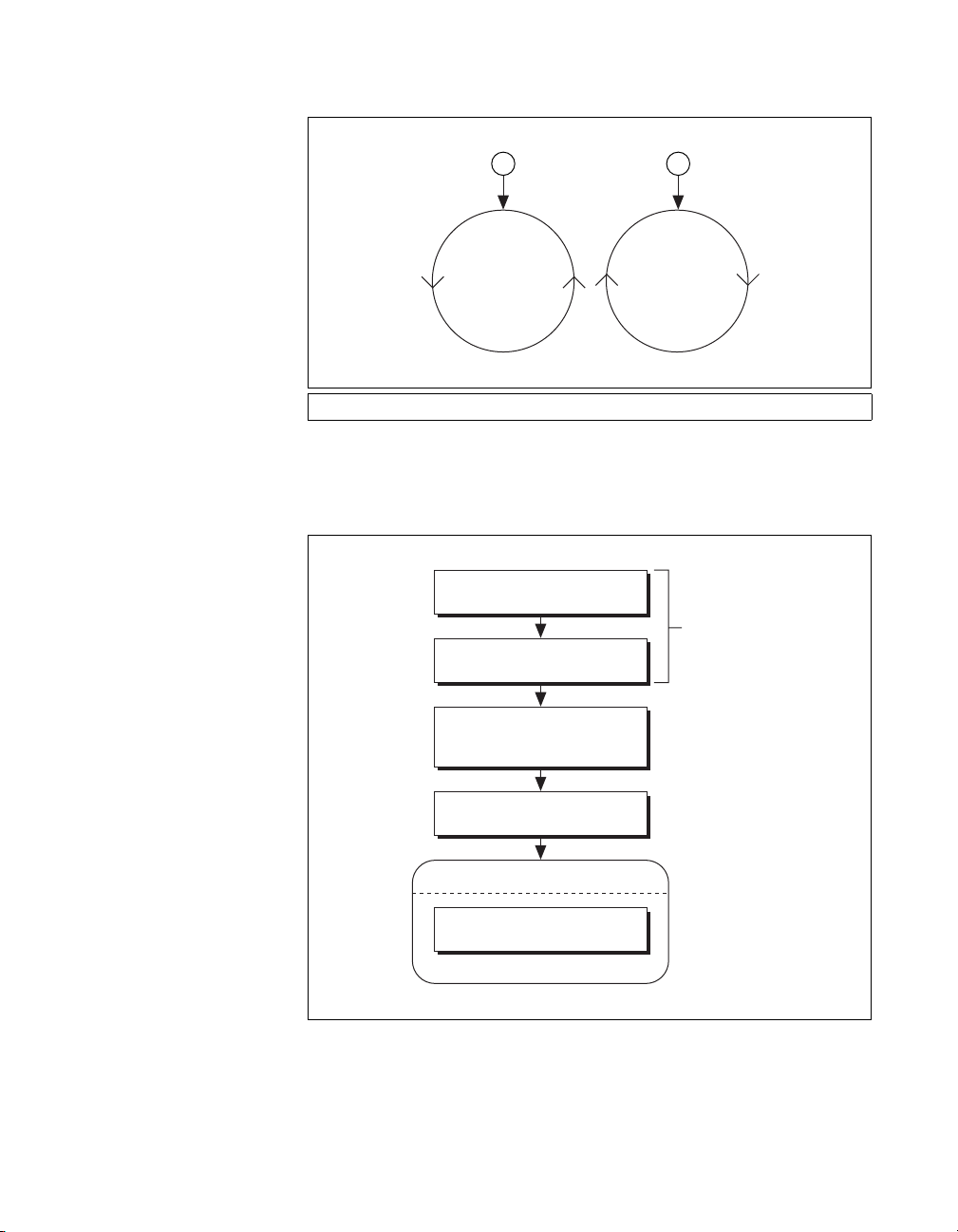
Arc Move Algorithm
Chapter 6 Arc Moves
1 2
1 Positive Travel Angle 2 Negative Travel Angle
Figure 6-3. Positive and Negative Travel Angles
Load Velocity
Move
Load Acceleration/
Deceleration
Load Circular Arc
Radius, Start Angle,
and Travel Angle
Start Motion
Loop Waiting for Move Complete
Perform Measurements
(Optional)
Constraints
Figure 6-4. Circular Arc Move Algorithm
© National Instruments Corporation 6-3 NI-Motion User Manual
Page 82

Chapter 6 Arc Moves
LabVIEW Code
5 6
4
1
1 Configure Vector Space
2 Load Velocity
3 Load Acceleration/Deceleration
4 Load Acceleration/Deceleration
C/C++ Code
The following example code is not necessarily complete, and may
not compile if copied exactly. Refer to the
NI-Motion CD for files that are complete and compile as is.
// Main Function
void main(void)
{
32
5 Load Circular Arc
6 Start Motion
7 Check Move Complete Status
7
98
8 Read per Axis Status
9 Read per Axis Status
10 Motion Error Handler
Figure 6-5. Circular Arc Move in LabVIEW
examples folder on the
u8 boardID;// Board identification number
u8 vectorSpace;// Vector space number
u16 csr = 0;// Communication status register
u16 axisStatus;// Axis status
u16 status;
u16 moveComplete;
//Variables for modal error handling
10
NI-Motion User Manual 6-4 ni.com
Page 83

Chapter 6 Arc Moves
u16 commandID;// The commandID of the function
u16 resourceID;// The resource ID
i32 errorCode;// Error code
///////////////////////////////
// Set the board ID
boardID = 1;
// Set the vector space number
vectorSpace = NIMC_VECTOR_SPACE1;
////////////////////////////////
// Configure a 2D vector space comprising of axes 1
and 2
err = flex_config_vect_spc(boardID, vectorSpace,
NIMC_AXIS1, NIMC_AXIS2, 0);
CheckError;
// Set the velocity for the move (in counts/sec)
err = flex_load_velocity(boardID, vectorSpace,
10000, 0xFF);
CheckError;
// Set the acceleration for the move (in
counts/sec^2)
err = flex_load_acceleration(boardID, vectorSpace,
NIMC_ACCELERATION, 100000, 0xFF);
CheckError;
// Set the deceleration for the move (in
counts/sec^2)
err = flex_load_acceleration(boardID, vectorSpace,
NIMC_DECELERATION, 100000, 0xFF);
CheckError;
// Load Spherical Arc
err = flex_load_circular_arc (boardID, vectorSpace,
5000/*radius*/, 0.0/*startAngle*/,
180.0/*travelAngle*/, 0xFF);
CheckError;
//Start the move
err = flex_start(boardID, vectorSpace, 0);
CheckError;
do
{
axisStatus = 0;
//Check the move complete status
© National Instruments Corporation 6-5 NI-Motion User Manual
Page 84

Chapter 6 Arc Moves
err = flex_check_move_complete_status(boardID,
vectorSpace, 0, &moveComplete);
CheckError;
// Check the following error/axis off status for
axis 1
err = flex_read_axis_status_rtn(boardID,
NIMC_AXIS1, &status);
CheckError;
axisStatus |= status;
// Check the following error/axis off status for
axis 2
err = flex_read_axis_status_rtn(boardID,
NIMC_AXIS2, &status);
CheckError;
axisStatus |= status;
// Read the communication status register and
check the modal // errors
err = flex_read_csr_rtn(boardID, &csr);
CheckError;
//Check the modal errors
if (csr & NIMC_MODAL_ERROR_MSG)
{
err = csr & NIMC_MODAL_ERROR_MSG;
CheckError;
}
}while (!moveComplete && !(axisStatus &
NIMC_FOLLOWING_ERROR_BIT) && !(axisStatus &
NIMC_AXIS_OFF_BIT));
//Exit on move complete/following error/axis off
return;// Exit the Application
//////////////////////
// Error Handling
//
nimcHandleError; //NIMCCATCHTHIS:
// Check to see if there were any Modal Errors
if (csr & NIMC_MODAL_ERROR_MSG){
do{
//Get the command ID, resource ID and the
error code of the //modal error from the
error stack on the device
NI-Motion User Manual 6-6 ni.com
Page 85

Spherical Arcs
Chapter 6 Arc Moves
flex_read_error_msg_rtn(boardID,&commandI
D,&resourceID, &errorCode);
nimcDisplayError(errorCode,commandID,res
ourceID);
//Read the communication status register
flex_read_csr_rtn(boardID,&csr);
}while(csr & NIMC_MODAL_ERROR_MSG);
}
else// Display regular error
nimcDisplayError(err,0,0);
return;// Exit the Application
}
A 3D spherical arc defines a 2D circular arc in the X'Y' plane of a
coordinate system that is transformed by rotation in pitch and yaw from the
normal 3D coordinate space (XYZ), as shown in Figures 6-6 and 6-7.
Z
Y
X
Figure 6-6. Changing Pitch by Rotating the X Axis
© National Instruments Corporation 6-7 NI-Motion User Manual
Page 86

Chapter 6 Arc Moves
Z
Y
X
Figure 6-7. Changing Yaw by Rotating the Z Axis
In the transformed X'Y'Z' space, the 3D arc is reduced to a simpler 2D arc.
The 3D arc is defined as a 2D circular arc in the X'Y' plane of a transformed
vector space X'Y'Z'. This transformed vector space, X'Y'Z', is defined in
orientation only, with no absolute position offset. Its orientation is relative
to the XYZ vector space, and is defined in terms of pitch and yaw angles.
When rotating through the pitch angle, the Y and Y' axes stay aligned with
each other while the X'Z' plane rotates around them. When rotating through
the yaw angle, the Y' axis never leaves the original XY plane, as the
newly-defined X'Y'Z' vector space rotates around the original Z-axis.
The radius, start angle, and travel angle parameters also apply to a spherical
arc that defines the arc in two dimensions.
NI-Motion User Manual 6-8 ni.com
Page 87

Algorithm
Load Velocity
Load Acceleration/
Deceleration
Load Spherical Arc
Radius, Start Angle,
Travel Angle, Yaw, and Pitch
Start Motion
Loop Waiting for Move Complete
Perform Measurements
(Optional)
Chapter 6 Arc Moves
Move
Constraints
Figure 6-8. Spherical Arc Algorithm
© National Instruments Corporation 6-9 NI-Motion User Manual
Page 88

Chapter 6 Arc Moves
LabVIEW Code
6
5
2
1
1 Configure Vector Space
2 Load Velocity
3 Load Acceleration/Deceleration
4 Load Acceleration/Deceleration
C/C++ Code
The following example code is not necessarily complete, and may
not compile if copied exactly. Refer to the
NI-Motion CD for files that are complete and compile as is.
// Main Function
void main(void)
{
4
3
7
5 Load Spherical Arc
6 Start Motion
7 Check Move Complete Status
8 Read per Axis Status
8
9
10
9 Read per Axis Status
10 Read per Axis Status
11 Motion Error Handler
Figure 6-9. Spherical Arc Move in LabVIEW
examples folder on the
u8 boardID;// Board identification number
u8 vectorSpace;// Vector space number
u16 csr = 0;// Communication status register
u16 axisStatus;// Axis status
u16 status;
u16 moveComplete;
//Variables for modal error handling
u16 commandID;// The commandID of the function
u16 resourceID;// The resource ID
i32 errorCode;// Error code
11
NI-Motion User Manual 6-10 ni.com
Page 89

Chapter 6 Arc Moves
///////////////////////////////
// Set the board ID
boardID = 1;
// Set the vector space number
vectorSpace = NIMC_VECTOR_SPACE1;
////////////////////////////////
// Configure a 3D vector space comprising of axes 1,
2 and 3
err = flex_config_vect_spc(boardID, vectorSpace,
NIMC_AXIS1, NIMC_AXIS2, NIMC_AXIS3);
CheckError;
// Set the velocity for the move (in counts/sec)
err = flex_load_velocity(boardID, vectorSpace,
10000, 0xFF);
CheckError;
// Set the acceleration for the move (in
counts/sec^2)
err = flex_load_acceleration(boardID, vectorSpace,
NIMC_ACCELERATION, 100000, 0xFF);
CheckError;
// Set the deceleration for the move (in
counts/sec^2)
err = flex_load_acceleration(boardID, vectorSpace,
NIMC_DECELERATION, 100000, 0xFF);
CheckError;
// Load Spherical Arc
err = flex_load_spherical_arc (boardID, vectorSpace,
5000/*radius*/, 45.0/*planePitch*/,
45.0/*planeYaw*/, 0.0/*startAngle*/,
180.0/*travelAngle*/, 0xFF);
CheckError;
//Start the move
err = flex_start(boardID, vectorSpace, 0);
CheckError;
do
{
axisStatus = 0;
//Check the move complete status
err = flex_check_move_complete_status(boardID,
vectorSpace, 0, &moveComplete);
CheckError;
© National Instruments Corporation 6-11 NI-Motion User Manual
Page 90

Chapter 6 Arc Moves
// Check the following error/axis off status for
axis 1
err = flex_read_axis_status_rtn(boardID,
NIMC_AXIS1, &status);
CheckError;
axisStatus |= status;
// Check the following error/axis off status for
axis 2
err = flex_read_axis_status_rtn(boardID,
NIMC_AXIS2, &status);
CheckError;
axisStatus |= status;
// Check the following error/axis off status for
axis 3
err = flex_read_axis_status_rtn(boardID,
NIMC_AXIS3, &status);
CheckError;
axisStatus |= status;
//Read the communication status register and
check the modal //errors
err = flex_read_csr_rtn(boardID, &csr);
CheckError;
//Check the modal errors
if (csr & NIMC_MODAL_ERROR_MSG)
{
err = csr & NIMC_MODAL_ERROR_MSG;
CheckError;
}
}while (!moveComplete && !(axisStatus &
NIMC_FOLLOWING_ERROR_BIT) && !(axisStatus &
NIMC_AXIS_OFF_BIT));
//Exit on move complete/following error/axis off
return;// Exit the Application
//////////////////////
// Error Handling
nimcHandleError; //NIMCCATCHTHIS:
// Check to see if there were any Modal Errors
if (csr & NIMC_MODAL_ERROR_MSG){
do{
NI-Motion User Manual 6-12 ni.com
Page 91

Helical Arcs
Chapter 6 Arc Moves
//Get the command ID, resource ID, and the
error code of the //modal error from the
error stack on the device
flex_read_error_msg_rtn(boardID,&commandI
D,&resourceID, &errorCode);
nimcDisplayError(errorCode,commandID,res
ourceID);
//Read the communication status register
flex_read_csr_rtn(boardID,&csr);
}while(csr & NIMC_MODAL_ERROR_MSG);
}
else// Display regular error
nimcDisplayError(err,0,0);
return;// Exit the Application
}
A helical arc defines an arc in a 3D coordinate space that consists of a circle
in the XY plane and synchronized linear travel in the Z-axis. The arc is
specified by a radius, start angle, travel angle, and Z-axis linear travel.
Linear travel is the linear distance traversed by the helical arc on the Z-axis,
as shown in Figure 6-10.
X
Z
4
Y
X
1 2 3
1 Side View of Helix 2 Top View of Helix 3 Isometric View of Helix 4 Linear Travel
Figure 6-10. Helical Arc
© National Instruments Corporation 6-13 NI-Motion User Manual
Z
X
Y
Page 92

Chapter 6 Arc Moves
Algorithm
Load Velocity
Move
Constraints
Load Acceleration/
Deceleration
Load Helical Arc
Radius, Start Angle,
Travel Angle, Linear Travel
Start Motion
Loop Waiting for Move Complete
Perform Measurements
(Optional)
Figure 6-11. Helical Arc Algorithm
NI-Motion User Manual 6-14 ni.com
Page 93

LabVIEW Code
Chapter 6 Arc Moves
6
5
1
2
1 Configure Vector Space
2 Load Velocity
3 Load Acceleration/Deceleration
4 Load Acceleration/Deceleration
C/C++ Code
The following example code is not necessarily complete, and may
not compile if copied exactly. Refer to the
NI-Motion CD for files that are complete and compile as is.
// Main Function
void main(void){
3 4
5 Load Helical Arc
6 Start Motion
7 Check Move Complete Status
8 Read per Axis Status
7
8
9
10
9 Read per Axis Status
10 Read per Axis Status
11 Motion Error Handler
Figure 6-12. Helical Arc Move in LabVIEW
examples folder on the
u8 boardID;// Board identification number
u8 vectorSpace;// Vector space number
u16 csr = 0;// Communication status register
u16 axisStatus;// Axis status
u16 status;
u16 moveComplete;
//Variables for modal error handling
u16 commandID;// The commandID of the function
u16 resourceID;// The resource ID
i32 errorCode;// Error code
///////////////////////////////
11
© National Instruments Corporation 6-15 NI-Motion User Manual
Page 94

Chapter 6 Arc Moves
// Set the board ID
boardID = 1;
// Set the vector space number
vectorSpace = NIMC_VECTOR_SPACE1;
////////////////////////////////
// Configure a 3D vector space comprising of axes 1,
2 and 3
err = flex_config_vect_spc(boardID, vectorSpace,
NIMC_AXIS1, NIMC_AXIS2, NIMC_AXIS3);
CheckError;
// Set the velocity for the move (in counts/sec)
err = flex_load_velocity(boardID, vectorSpace,
10000, 0xFF);
CheckError;
// Set the acceleration for the move (in
counts/sec^2)
err = flex_load_acceleration(boardID, vectorSpace,
NIMC_ACCELERATION, 100000, 0xFF);
CheckError;
// Set the deceleration for the move (in
counts/sec^2)
err = flex_load_acceleration(boardID, vectorSpace,
NIMC_DECELERATION, 100000, 0xFF);
CheckError;
// Load Helical Arc
err = flex_load_helical_arc (boardID, vectorSpace,
5000/*radius*/, 0.0/*startAngle*/,
720.0/*travelAngle*/, 5000 /*linear travel*/, 0xFF);
CheckError;
//Start the move
err = flex_start(boardID, vectorSpace, 0);
CheckError;
do
{
axisStatus = 0;
//Check the move complete status
err = flex_check_move_complete_status(boardID,
vectorSpace, 0, &moveComplete);
CheckError;
// Check the following error/axis off status for
axis 1
NI-Motion User Manual 6-16 ni.com
Page 95

Chapter 6 Arc Moves
err = flex_read_axis_status_rtn(boardID,
NIMC_AXIS1, &status);
CheckError;
axisStatus |= status;
// Check the following error/axis off status for
axis 2
err = flex_read_axis_status_rtn(boardID,
NIMC_AXIS2, &status);
CheckError;
axisStatus |= status;
// Check the following error/axis off status for
axis 3
err = flex_read_axis_status_rtn(boardID,
NIMC_AXIS3, &status);
CheckError;
axisStatus |= status;
//Read the communication status register and
check the modal //errors
err = flex_read_csr_rtn(boardID, &csr);
CheckError;
//Check the modal errors
if (csr & NIMC_MODAL_ERROR_MSG)
{
err = csr & NIMC_MODAL_ERROR_MSG;
CheckError;
}
}while (!moveComplete && !(axisStatus &
NIMC_FOLLOWING_ERROR_BIT) && !(axisStatus &
NIMC_AXIS_OFF_BIT));
//Exit on move complete/following error/axis off
return;// Exit the Application
//////////////////////
// Error Handling
//
nimcHandleError; //NIMCCATCHTHIS:
// Check to see if there were any Modal Errors
if (csr & NIMC_MODAL_ERROR_MSG){
do{
//Get the command ID, resource ID, and the
error code of the //modal error from the
error stack on the device
© National Instruments Corporation 6-17 NI-Motion User Manual
Page 96

Chapter 6 Arc Moves
flex_read_error_msg_rtn(boardID,&commandI
D,&resourceID, &errorCode);
nimcDisplayError(errorCode,commandID,res
ourceID);
//Read the communication status register
flex_read_csr_rtn(boardID,&csr);
}while(csr & NIMC_MODAL_ERROR_MSG);
}
else// Display regular error
nimcDisplayError(err,0,0);
return;// Exit the Application
}
NI-Motion User Manual 6-18 ni.com
Page 97

Contoured Moves
A contoured move moves an axis or a coordinate space of axes in a pattern
that you define. The trajectory generator on the motion controller is not
used during a contoured move. The controller takes position data in the
form of an array, and splines the data before outputting it to the DACs or
stepper outputs, as shown in Figure 7-1.
7
Overview
User-Defined
Points
Figure 7-1. Contoured Move Data Path
All positions in a contouring buffer are relative to the current position when
starting. There is an assumed 0 point that the firmware adds to the front of
the buffer of points. For example, if the contour buffer is [10, 20, 30, 40],
the positions are [0, 10, 20, 30, 40] in the firmware.
When a contour move starts it takes a snap shot of the current position
according to the following equation:
StartPosition = currentPosition.
The start position is added to each point in the buffer to get the actual
position to move through according to the following equation:
Point = StartPosition + bufferPosition[n].
If the current position is 100, and the buffer is [10, 20, 30, 40], the contour
move follows these points: [100, 110, 120, 130, 140].
Cubic Spine
Output to DACs or
Stepper Output
© National Instruments Corporation 7-1 NI-Motion User Manual
Page 98

Chapter 7 Contoured Moves
The difference between absolute contouring and relative contouring is how
the points in the buffer are treated. The previous example was of an absolute
contour move. A relative contour move treats the points as deltas according
to the following formula:
Point[n] = Point[n-1] + bufferPosition[n]
For a relative contour move that starts at position 100 and includes a buffer
with the following values: [10, 20, 30, 40], the points the contour move
follows are [100, 110, 130, 160, 200].
For contoured moves, no two consecutive points can differ by more than
15
2
– 1. For absolute position mode, the first position in the array passed to
the controller must be less than 2
must be less than 2
15
controller can be greater than 2
Arbitrary Contoured Moves
Contoured moves are useful when you want to generate a trajectory that
cannot be constructed from straight lines and arcs. To ensure that the
motion is smooth with minimum jerk, the motion controller creates
intermediate points using a cubic spline algorithm.
15
– 1, and any two consecutive points
– 1. For relative position mode, no point passed to the
15
– 1.
The move constraints commonly used to limit other types of moves, such
as maximum velocity, maximum acceleration, maximum deceleration,
and maximum jerk, have no effect on contoured moves. However, the
NI Motion Assistant prototyping tool can remap a user-defined trajectory
based on specified move constraints, preserving move characteristics and
move geometry.
NI-Motion User Manual 7-2 ni.com
Page 99

Contoured Move Algorithm
Set Operation Mode
Specify absolute or
relative contouring
Configure the buffer
on the device
Write Buffer
Write the array of points and the
number of points you are writing
Start Motion
Loop Waiting for Move Complete
Update Contoured Data (Optional)
Chapter 7 Contoured Moves
• Set the Buffer Type as Position
• Total Points is the total number of
countoured points you want to load
• Buffer Size is the size of the buffer you
want to create on the device
• Set Old Data Stop to TRUE if you do
not want old data to be used
• Requested Interval is the time interval
between points
Check the buffer on the device
Number of points consumed
Write Buffer
Write remaining points
to onboard buffer
Perform Measurements
(Optional)
Clear the buffer that stores
contoured move points
Restore Operation Mode
Set operation mode back to absolute
position to clear contouring data
Figure 7-2. Contoured Move Algorithm
© National Instruments Corporation 7-3 NI-Motion User Manual
Page 100

Chapter 7 Contoured Moves
All contoured moves are relative, meaning motion starts from the position
of the axis or axes at the time the contouring move starts. This behavior is
similar to the way arc moves work. Depending on the operation mode you
use, you can load absolute positions in the array or relative positions, which
imply incremental position differences between contouring points.
Absolute versus Relative Contouring
If an axis starts at position 0 and uses either of the following sets of
contouring points, the axis ends up at position 28. If the axis starts at
position 10, it ends up at position 38 in both cases.
13610141822252728
Figure 7-3. Absolute Contouring Buffer Values
1234444321
Figure 7-4. Relative Contouring Buffer Values
NI-Motion User Manual 7-4 ni.com
 Loading...