National Instruments 370760B-01 User Manual

TM

MATRIXx

XmathTM Xµ Manual

MATRIXx Xmath Basics

The MATRIXx products and related items have been purchased from Wind
River Systems, Inc. (formerly Integrated Systems, Inc.). These reformatted user
materials may contain references to those entities. Any trademark or copyright
notices to those entities are no longer valid and any references to those entities
as the licensor to the MATRIXx products and related items should now be
considered as referring to National Instruments Corporation.

National Instruments did not acquire RealSim hardware (AC-1000, AC-104,
PCI Pro) and does not plan to further develop or support RealSim software.

NI is directing users who wish to continue to use RealSim software and hardware
to third parties. The list of NI Alliance Members (third parties) that can provide
RealSim support and the parts list for RealSim hardware are available in our
online KnowledgeBase. You can access the KnowledgeBase at

www.ni.com/support.

NI plans to make it easy for customers to target NI software and hardware,
including LabVIEW real-time and PXI, with MATRIXx in the future.
For information regarding NI real-time products, please visit

www.ni.com/realtime or contact us at [e-mail].

April 2004 Edition

Part Number 370760B-01

Support

Worldwide Technical Support and Product Information

ni.com

National Instruments Corporate Headquarters

11500 North Mopac Expressway Austin, Texas 78759-3504 USA Tel: [phone]

Worldwide Offices

Australia 1800 300 800, Austria 43 0 662 45 79 90 0, Belgium 32 0 2 757 00 20, Brazil 55 11 3262 3599,
Canada (Calgary) 403 274 9391, Canada (Ottawa) 613 233 5949, Canada (Québec) 450 510 3055,
Canada (Toronto) 905 785 0085, Canada (Vancouver) 514 685 7530, China 86 21 6555 7838,
Czech Republic 420 224 235 774, Denmark 45 45 76 26 00, Finland 385 0 9 725 725 11, France 33 0 1 48 14 24 24,
Germany 49 0 89 741 31 30, Greece 30 2 10 42 96 427, India 91 80 51190000, Israel 972 0 3 6393737,
Italy 39 02 413091, Japan 81 3 5472 2970, Korea 82 02 3451 3400, Malaysia 603 9131 0918, Mexico 001 800 010 0793,
Netherlands 31 0 348 433 466, New Zealand 0800 553 322, Norway 47 0 66 90 76 60, Poland 48 22 3390150,
Portugal 351 210 311 210, Russia 7 095 783 68 51, Singapore 65 6226 5886, Slovenia 386 3 425 4200,
South Africa 27 0 11 805 8197, Spain 34 91 640 0085, Sweden 46 0 8 587 895 00, Switzerland 41 56 200 51 51,
Taiwan 886 2 2528 7227, Thailand 662 992 7519, United Kingdom 44 0 1635 523545

For further support information, refer to the Technical Support Resources and Professional Services appendix. To comment
on the documentation, send email to [e-mail].

© 2000–2003 National Instruments Corporation. All rights reserved.

Important Information

Warranty

The media on which you receive National Instruments software are warranted not to fail to execute programming instructions, due to defects
in materials and workmanship, for a period of 90 days from date of shipment, as evidenced by receipts or other documentation. National
Instruments will, at its option, repair or replace software media that do not execute programming instructions if National Instruments receives
notice of such defects during the warranty period. National Instruments does not warrant that the operation of the software shall be
uninterrupted or error free.

A Return Material Authorization (RMA) number must be obtained from the factory and clearly marked on the outside of the package before
any equipment will be accepted for warranty work. National Instruments will pay the shipping costs of returning to the owner parts which are
covered by warranty.

National Instruments believes that the information in this document is accurate. The document has been carefully reviewed for technical
accuracy. In the event that technical or typographical errors exist, National Instruments reserves the right to make changes to subsequent
editions of this document without prior notice to holders of this edition. The reader should consult National Instruments if errors are suspected.
In no event shall National Instruments be liable for any damages arising out of or related to this document or the information contained in it.

E

XCEPT AS SPECIFIED HEREIN, NATIONAL INSTRUMENTS MAKES NO WARRANTIES, EXPRESS OR IMPLIED, AND SPECIFICALLY DISCLAIMS ANY WARRANTY OF

MERCHANTABILITY OR FITNESS FOR A PARTICULAR PURPOSE . CUSTOMER’S RIGHT TO RECOVER DAMAGES CAUSED BY FAULT OR NEGLIGENCE ON THE PART OF

N

ATIONAL INSTRUMENTS SHALL BE LIMITED TO THE AMOUNT THERETOFORE PAID BY THE CUSTOMER. NATIONAL INSTRUMENTS WILL NOT BE LIABLE FOR
DAMAGES RESULTING FROM LOSS OF DATA, PROFITS, USE OF PRODUCTS, OR INCIDENTAL OR CONSEQUENTIAL DAMAGES, EVEN IF ADVISED OF THE PO SSIBILITY
THEREOF. This limitation of the liability of National Instruments will apply regardless of the form of action, whether in contract or tort, including

negligence. Any action against National Instruments must be brought within one year after the cause of action accrues. National Instruments
shall not be liable for any delay in performance due to causes beyond its reasonable control. The warranty provided herein does not cover
damages, defects, malfunctions, or service failures caused by owner’s failure to follow the National Instruments installation, operation, or
maintenance instructions; owner’s modification of the product; owner’s abuse, misuse, or negligent acts; and power failure or surges, fire,
flood, accident, actions of third parties, or other events outside reasonable control.

Copyright

Under the copyright laws, this publication may not be reproduced or transmitted in any form, electronic or mechanical, including photocopying,
recording, storing in an information retrieval system, or translating, in whole or in part, without the prior written consent of National
Instruments Corporation.

Trademarks

LabVIEW™, MATRIXx™, National Instruments™, NI™, ni.com™, SystemBuild™, and Xmath™ are trademarks of National Instruments
Corporation.

Product and company names mentioned herein are trademarks or trade names of their respective companies.

Patents

For patents covering National Instruments products, refer to the appropriate location: Help»Patents in your software, the patents.txt file
on your CD, or

ni.com/patents.

WARNING REGARDING USE OF NATIONAL INSTRUMENTS PRODUCTS

(1) NATIONAL INSTRUMENTS PRODUCTS ARE NOT DESIGNED WITH COMPONENTS AND TESTING FOR A LEVEL OF
RELIABILITY SUITABLE FOR USE IN OR IN CONNECTION WITH SURGICAL IMPLANTS OR AS CRITICAL COMPONENTS IN
ANY LIFE SUPPORT SYSTEMS WHOSE FAILURE TO PERFORM CAN REASONABLY BE EXPECTED TO CAUSE SIGNIFICANT
INJURY TO A HUMAN.

(2) IN ANY APPLICATION, INCLUDING THE ABOVE, RELIABILITY OF OPERATION OF THE SOFTWARE PRODUCTS CAN BE
IMPAIRED BY ADVERSE FACTORS, INCLUDING BUT NOT LIMITED TO FLUCTUATIONS IN ELECTRICAL POWER SUPPLY,
COMPUTER HARDWARE MALFUNCTIONS, COMPUTER OPERATING SYSTEM SOFTWARE FITNESS, FITNESS OF COMPILERS
AND DEVELOPMENT SOFTWARE USED TO DEVELOP AN APPLICATION, INSTALLATION ERRORS, SOFTWARE AND
HARDWARE COMPATIBILITY PROBLEMS, MALFUNCTIONS OR FAILURES OF ELECTRONIC MONITORING OR CONTROL
DEVICES, TRANSIENT FAILURES OF ELECTRONIC SYSTEMS (HARDWARE AND/OR SOFTWARE), UNANTICIPATED USES OR
MISUSES, OR ERRORS ON THE PART OF THE USER OR APPLICATIONS DESIGNER (ADVERSE FACTORS SUCH AS THESE ARE
HEREAFTER COLLECTIVELY TERMED “SYSTEM FAILURES”). ANY APPLICATION WHERE A SYSTEM FAILURE WOULD
CREATE A RISK OF HARM TO PROPERTY OR PERSONS (INCLUDING THE RISK OF BODILY INJURY AND DEATH) SHOULD
NOT BE RELIANT SOLELY UPON ONE FORM OF ELECTRONIC SYSTEM DUE TO THE RISK OF SYSTEM FAILURE. TO AVOID
DAMAGE, INJURY, OR DEATH, THE USER OR APPLICATION DESIGNER MUST TAKE REASONABLY PRUDENT STEPS TO
PROTECT AGAINST SYSTEM FAILURES, INCLUDING BUT NOT LIMITED TO BACK-UP OR SHUT DOWN MECHANISMS.
BECAUSE EACH END-USER SYSTEM IS CUSTOMIZED AND DIFFERS FROM NATIONAL INSTRUMENTS' TESTING
PLATFORMS AND BECAUSE A USER OR APPLICATION DESIGNER MAY USE NATIONAL INSTRUMENTS PRODUCTS IN
COMBINATION WITH OTHER PRODUCTS IN A MANNER NOT EVALUATED OR CONTEMPLATED BY NATIONAL
INSTRUMENTS, THE USER OR APPLICATION DESIGNER IS ULTIMATELY RESPONSIBLE FOR VERIFYING AND VALIDATING
THE SUITABILITY OF NATIONAL INSTRUMENTS PRODUCTS WHENEVER NATIONAL INSTRUMENTS PRODUCTS ARE
INCORPORATED IN A SYSTEM OR APPLICATION, INCLUDING, WITHOUT LIMITATION, THE APPROPRIATE DESIGN,
PROCESS AND SAFETY LEVEL OF SUCH SYSTEM OR APPLICATION.

Contents

1 Introduction 1

1.1 Notation..................................... 1

1.2 Manual Outline . . . . . . . . . . . . . . . . . . . . . . . . . . . . . . . . . 2

1.3 How to avoid really reading this Manual . . . . . . . . . . . . . . . . . . . 3

2 Overview of the Underlying Theory 5

2.1 Introduction................................... 5

2.1.1 Notation................................. 6

2.1.2 AnIntroductiontoNorms....................... 8

2.2 Modeling Uncertain Systems . . . . . . . . . . . . . . . . . . . . . . . . . 13

2.2.1 Perturbation Models for Robust Control . . . . . . . . . . . . . . . 13

2.2.2 Linear Fractional Transformations . . . . . . . . . . . . . . . . . . 17

2.2.3 Assumptions on P ,∆,andtheunknownsignals .......... 22

2.2.4 Additional Perturbation Structures . . . . . . . . . . . . . . . . . . 23

iii

iv CONTENTS

2.2.5 Obtaining Robust Control Models for Physical Systems . . . . . . 28

2.3 H

and H2DesignMethodologies ...................... 29

∞

2.3.1 H

2.3.2 Assumptions for the H

DesignOverview ......................... 31

∞

DesignProblem .............. 32

∞

2.3.3 A Brief Review of the Algebraic Riccati Equation . . . . . . . . . . 33

2.3.4 Solving the H

2.3.5 Further Notes on the H

2.3.6 H

DesignOverview.......................... 40

2

2.3.7 Details of the H

Design Problem for a Special Case . . . . . . . . . 36

∞

Design Algorithm . . . . . . . . . . . . . 38

∞

DesignProcedure ................. 40

2

2.4 µ Analysis.................................... 42

2.4.1 MeasuresofPerformance ....................... 42

2.4.2 Robust Stability and µ ......................... 44

2.4.3 RobustPerformance .......................... 46

2.4.4 Properties of µ ............................. 47

2.4.5 TheMainLoopTheorem ....................... 49

2.4.6 State-spaceRobustnessAnalysisTests................ 51

2.4.7 Analysis with both Real and Complex Perturbations . . . . . . . . 58

2.5 µ Synthesis and D-K Iteration ........................ 58

2.5.1 µ-Synthesis ............................... 58

2.5.2 The D-K Iteration Algorithm . . . . . . . . . . . . . . . . . . . . . 60

CONTENTS v

2.6 ModelReduction................................ 64

2.6.1 Truncation and Residualization . . . . . . . . . . . . . . . . . . . . 65

2.6.2 BalancedTruncation.......................... 65

2.6.3 HankelNormApproximation ..................... 68

3 Functional Description of Xµ 71

3.1 Introduction................................... 71

3.2 DataObjects .................................. 71

3.2.1 Dynamic Systems .......................... 72

3.2.2 pdms................................... 74

3.2.3 Subblocks: selecting input & outputs . . . . . . . . . . . . . . . . . 77

3.2.4 BasicFunctions............................. 78

3.2.5 Continuous to Discrete Transformations . . . . . . . . . . . . . . . 81

3.3 MatrixInformation,DisplayandPlotting .................. 81

3.3.1 Information Functions for Data Objects . . . . . . . . . . . . . . . 81

3.3.2 FormattedDisplayFunctions ..................... 82

3.3.3 PlottingFunctions ........................... 82

3.4 SystemResponseFunctions .......................... 85

3.4.1 CreatingTimeDomainSignals .................... 85

3.4.2 Dynamic System TimeResponses ................. 85

3.4.3 FrequencyResponses.......................... 88

vi CONTENTS

3.5 SystemInterconnection ............................ 91

3.6 H

and H∞AnalysisandSynthesis...................... 95

2

3.6.1 ControllerSynthesis .......................... 95

3.6.2 SystemNormCalculations ...................... 105

3.7 Structured Singular Value (µ) Analysis and Synthesis . . . . . . . . . . . 107

3.7.1 Calculation of µ ............................ 107

3.7.2 The D-K Iteration........................... 110

3.7.3 Fitting D Scales ............................ 112

3.7.4 Constructing Rational Perturbations . . . . . . . . . . . . . . . . . 120

3.7.5 BlockStructuredNormCalculations................. 121

3.8 ModelReduction................................ 121

3.8.1 Truncation and Residualization . . . . . . . . . . . . . . . . . . . . 122

3.8.2 BalancedRealizations ......................... 123

3.8.3 Hankel Singular Value Approximation . . . . . . . . . . . . . . . . 125

4 Demonstration Examples 127

4.1 TheHimatExample .............................. 127

4.1.1 ProblemDescription.......................... 127

4.1.2 State-spaceModelofHimat...................... 128

4.1.3 Creating a Weighted Interconnection Structure for Design . . . . . 131

4.1.4 H

Design ............................... 133

∞

CONTENTS vii

4.1.5 µ Analysis of the H

Controller ................... 138

∞

4.1.6 Fitting D-scales for the D-K Iteration................ 140

4.1.7 DesignIteration#2 .......................... 143

4.1.8 Simulation Comparison with a Loopshaping Controller . . . . . . . 146

4.2 A Simple Flexible Structure Example . . . . . . . . . . . . . . . . . . . . 153

4.2.1 TheControlDesignProblem ..................... 153

4.2.2 Creating the Weighted Design Interconnection Structure . . . . . . 155

4.2.3 Design of an H

Controller...................... 162

∞

4.2.4 RobustnessAnalysis .......................... 165

4.2.5 D-K Iteration ............................. 168

4.2.6 ASimulationStudy .......................... 173

5 Bibliography 192

6 Function Reference 201

6.1 Xµ Functions .................................. 201

6.2 Xµ Subroutines and Utilities . . . . . . . . . . . . . . . . . . . . . . . . . 377

Appendices 391

A Translation Between Matlab µ-Tools and Xµ ............... 391

A.1 DataObjects .............................. 392

A.2 Matrix Information, Display and Plotting . . . . . . . . . . . . . . 397

viii CONTENTS

A.3 SystemResponseFunctions...................... 398

A.4 SystemInterconnection ........................ 399

A.5 ModelReduction............................ 399

A.6 H

and H∞AnalysisandSynthesis ................. 399

2

A.7 Structured Singular Value (µ) Analysis and Synthesis . . . . . . . 400

Chapter 1

Introduction

Xµ is a suite of Xmath functions for the modeling, analysis and synthesis of linear
robust control systems. Robust control theory has developed rapidly during the last
decade to the point where a useful set of computational tools can be used to solve a wide
range of control problems. This theory has already been applied to a wide range of
practical problems.

This manual describes the Xµ functions and presents a demonstration of their
application. The underlying theory is outlined here and further theoretical details can
be found in the many references provided.

It is assumed that the reader is familiar with the use of Xmath; the Xmath Basics
manual and the on-line demos are a good way of getting started with Xmath. A good
knowledge of control theory and application is also assumed. The more that is known
about robust control theory the better as the details are not all covered here.

1.1 Notation

Several font types or capitalization styles are used to distinguish between data objects.
The following table lists the various meanings.

1

2 CHAPTER 1. INTRODUCTION

Notation Meaning

pdm Xmath parameter dependent matrix data object
Dynamic System Xmath dynamic system data object

Code examples and function names are set in typewriter font to distinguish them from
narrative text.

1.2 Manual Outline

Chapter 2 outlines the applicable robust control theory. Perturbation models and linear
fractional transformations form the basis of the modeling framework. The discussion is
aimed at an introductory level and not all of the subtleties are covered. The theory
continues with an overview of the H
elsewhere for detail of the theory. The robust control methodology covered here is based
on the analysis of systems with perturbations. This is covered in some detail as such an
understanding is required for effective use of this software. Repeated analysis can be
used to improve upon the synthesis; this takes us from the standard H
to the more sophisticated µ-synthesis techniques.

design technique. Again the reader is referred

∞

design method

∞

The translation between the theoretical concepts and the use of the software is made in
Chapter 3. The means of performing typical robust control calculations are discussed in
some detail. This chapter also serves to introduce the Xµ functions. The discussion is
extended to include some of the relevant Xmath functions. A prior reading of Chapter 2
is helpful for putting this material in context.

The best means of getting an idea of the use of the software is to study completed design
examples, given in Chapter 4. These currently includes a design study for an aerospace
application. Typical modeling, analysis, synthesis, and simulation studies are illustrated.
These studies can be used as initial templates for the user’s application.

Chapter 6 is a function reference guide containing a formal description of each function.
This is similar to that given via the on-line help capability. Functions are listed in
relevant groupings at the start of the chapter. This gives an overview of some of the
software capabilities.

1.3. HOW TO AVOID REALLY READING THIS MANUAL 3

1.3 How to avoid really reading this Manual

The layout of the manual proceeds from introduction to background to syntax detail to
application descriptions. This may be tediously theoretical for some. If you are one of
those that considers reading the manual as the option of last resort
the applications (Chapter 4). If you have no prior Xmath experience then skimming
through Chapter 3 is essential. After running the demos and getting a feel for what the
software can do look briefly through the theory section.

1

then go directly to

1

And it seems that you are now exercising that option

Chapter 2

Overview of the Underlying
Theory

2.1 Introduction

The material covered here is taken from a variety of sources. The basic approach is
described by Doyle [1, 2], and further elaborated upon by Packard [3]. Summaries have
also appeared in work by Smith [4] and others.

Motivating background can be found in the early paper by Doyle and Stein [5]. An
overview of the robust control approach, particularly for process control systems, is
given by Morari and Zafiriou [6]. The reader can also find a description of the H
synthesis robust control approach in [7].

/µ

∞

There are a number of descriptions of this approach to practical problems. In the last
few years a significant number of these have been described in the proceedings of the
American Control Conference (ACC) and the IEEE Control and Decision Conference
(CDC). Only some of the early illustrative examples are cited here.

Application of µ synthesis to a shuttle control subsystem is given by Doyle et al. [8].
Examples of flexible structure control are described by Balas and
coworkers [9, 10, 11, 12] and Smith, Fanson and Chu [13, 14]. There have also been

5

6 CHAPTER 2. OVERVIEW OF THE UNDERLYING THEORY

several studies involving process control applications, particularly high purity distillation
columns. These are detailed by Skogestad and Morari in [15, 16, 17, 18]

Section 2.2 introduces robust control perturbation models and linear fractional
transformations. Weighted H

design is covered in Section 2.3. The analysis of closed

∞

loop systems with the structured singular value (µ) is overviewed in Section 2.4.
Section 2.5 discusses µ synthesis and the D-K iteration. Model reduction is often used
to reduce the controller order prior to implementation and this is covered in Section 2.6.

2.1.1 Notation

We will use some fairly standard notation and this is given here for reference.

R set of real numbers
C set of complex numbers

n

R

n

C

n×m

R

n×m

C

I

n

0 matrix (or vector or scalar) of zeros of appropriate dimension

set of real valued vectors of dimension n × 1
set of complex valued vectors of dimension n × 1
set of real valued matrices of dimension n × m
set of complex valued matrices of dimension n × m
identity matrix of dimension n × n

The following apply to a matrix, M ∈C

M
M

T

∗

transpose of M
complex conjugate transpose of M

n×m

.

|M| absolute value of each element of M (also applies if M is a vector or scalar)
Re{M} real part of M
Im{M} imaginary part of M
dim(M) dimensions of M

σ

(M) maximum singular value of M

max

(M) minimum singular value of M

σ

min

M

ij

element of M in row i, column j. (also used for the i,j partition of a previously defined

partition of M)

(M) an eigenvalue of M

λ

i

ρ(M) spectral radius (max

i|λi

(M)|)

kMk norm of M (see section 2.1.2 for more details)

2.1. INTRODUCTION 7

-

z v

 

y

P

P

11

21



P

P

12

22



u

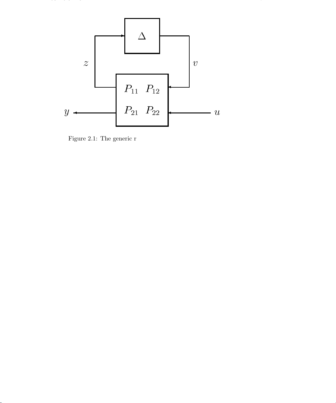
Figure 2.1: The generic robust control model structure

P

n

Trace(M) trace of M (

i=1

Mii)

Block diagrams will be used to represent interconnections of systems. Consider the
example feedback interconnection shown in Fig. 2.1. Notice that P has been partitioned
into four parts. This diagram represents the equations,

z = P
y = P

v + P12u

11

v + P22u

21

v =∆z.

This type of diagram (and the associated equations) will be used whenever the objects

P , z, y, etc., are well defined and compatible. For example P could be a matrix and z,
y, etc., would be vectors. If P represented a dynamic system then z, y, etc., would be

signals and

y = P

v + P22u,

21

8 CHAPTER 2. OVERVIEW OF THE UNDERLYING THEORY

is interpreted to mean that the signal y is the sum of the response of system P
input signal v and system P

to input signal u. In general, we will not be specific about

22

to

21

the representation of the system P . If we do need to be more specific about P ,then
P(s) is the Laplace representation and p(t) is the impulse response.

Note that Figure 2.1 is drawn from right to left. We use this form of diagram because it
more closely represents the order in which the systems are written in the corresponding
mathematical equations. We will later see that the particular block diagram shown in
Figure 2.1 is used as a generic description of a robust control system.

In the case where we are considering a state-space representation, the following notation
is also used. Given P(s), with state-space representation,

sx(s)=Ax(s)+Bu(s)

y(s)=Cx(s)+Du(s),

we associate this description with the notation,



P (s)=

A

B

C D



.

The motivation for this notation comes from the example presented in Section 2.2.4. We
will also use this notation to for state-space representation of discrete time systems
(where s in the above is replaced by z). The usage will be clear from the context of the
discussion.

2.1.2 An Introduction to Norms

A norm is simply a measure of the size of a vector, matrix, signal, or system. We will
define and concentrate on particular norms for each of these entities. This gives us a
formal way of assessing whether or not the size of a signal is large or small enough. It
allows us to quantify the performance of a system in terms of the size of the input and
output signals.

Unless stated otherwise, when talking of the size of a vector, we will be using the

2.1. INTRODUCTION 9

Euclidean norm. Given,





x

1





.

x =

.



,



.

x

n

the Euclidean (or 2-norm) of x, denoted by kxk, is defined by,

!

|xi|

1/2

.

n

kxk =

X

i=1

Many other norms are also options; more detail on the easily calculated norms can be
found in the on-line help for the norm function. The term spatial-norm is often applied
when we are looking at norms over the components of a vector.

Now consider a vector valued signal,

x(t)=






x

x

1

n

(t)
.

.
.

(t)






.

As well as the issue of the spatial norm, we now have the issue of a time norm. In the
theory given here, we concentrate on the 2-norm in the time domain. In otherwords,

kx

(t)k =

i



Z

∞

−∞

|xi(t)|2dt



1/2

.

This is simply the energy of the signal. This norm is sometimes denoted by a subscript
of two, i.e. kx

(t)k2. Parseval’s relationship means that we can also express this norm in

i

the Laplace domain as follows,

kx

(s)k =

i



Z

∞

1

2π

|xi(ω)|2dω

−∞



1/2

.

10 CHAPTER 2. OVERVIEW OF THE UNDERLYING THEORY

For persistent signals, where the above norm is unbounded, we can define a power norm,

!

1/2

. (2.1)

(t)k = lim

kx

i

T →∞

2T

Z

T

1

|xi(t)|2dt

−T

The above norms have been defined in terms of a single component, x

(t), of a vector

i

valued signal, x(t). The choice of spatial norm determines how we combine these
components to calculate kx(t)k. We can mix and match the spatial and time parts of the
norm of a signal. In practice it usually turns out that the choice of the time norm is
more important in terms of system analysis. Unless stated otherwise, kx(t)k implies the
Euclidean norm spatially and the 2-norm in the time direction.

Certain signal spaces can be defined in terms of their norms. For example, the set of
signals x(t), with kx(t)k




L

=x(t)

2



kx(t)k < ∞.



finite is denoted by L2. The formal definition is,

2

A similar approach can be taken in the discrete-time domain. Consider a sequence,

∞

{x(k)}

, with 2-norm given by,

k=0

∞

X

kx(k)k

=

2

|x(k)|

k=0

!

1/2

2

.

A lower case notation is used to indicate the discrete-time domain. All signals with finite
2-norm are therefore,




l

=x(k),k =0,...,∞

2

We can essentially split the space L
elements of L

which are analytic in the right-half plane. This can be thought of as

2



kx(k)k2<∞.



into two pieces, H2and H

2

⊥

. H2is the set of

2

those which have their poles strictly in the left half plane; i.e. all stable signals.

⊥

Similarly, H

are all signal with their poles in the left half plane; all strictly unstable

2

2.1. INTRODUCTION 11

signals. Strictly speaking, signals in H

2

or H

are not defined on the ω axis. However

2

⊥

we usually consider them to be by taking a limit as we approach the axis.

A slightly more specialized set is RL
strictly proper functions with no poles on the imaginary axis. Similarly we can consider

as strictly proper stable functions and RH

RH

2

poles in Re(s)< 0. The distinction between RL

, the set of real rational functions in L2. These are

2

⊥

as strictly proper functions with no

2

and L2is of little consequence for the

2

sorts of analysis we will do here.

The concept of a unit ball will also come up in the following sections. This is simply the
set of all signals (or vectors, matrices or systems) with norm less than or equal to one.
The unit ball of L

=x(t)

BL

2

, denoted by BL2, is therefore defined as,

2





kx(t)k2< 1.



Now let’s move onto norms of matrices and systems. As expected the norm of a matrix
gives a measure of its size. We will again emphasize only the norms which we will
consider in the following sections. Consider defining a norm in terms of the maximum
gain of a matrix or system. This is what is known as an induced norm. Consider a
matrix, M , and vectors, u and y,where

y=Mu.

Define, kM k,by

kyk

kMk=max

u,kuk<∞

kuk

.

Because M is obviously linear this is equivalent to,

kMk =max

u,kuk=1

kyk.

The properties of kMk will depend on how we define the norms for the vectors u and y.
If we choose our usual default of the Euclidean norm then kMk is given by,

kMk = σ

max

(M),

12 CHAPTER 2. OVERVIEW OF THE UNDERLYING THEORY

where σ

denotes the maximum singular value. Not all matrix norms are induced

max

from vector norms. The Froebenius norm (square root of the sum of the squares of all
matrix elements) is one such example.

Now consider the case where P(s) is a dynamic system and we define an induced norm
from L

to L2as follows. In this case, y(s) is the output of P (s)u(s)and

2

ky(s)k

kP(s)k=max

u(s)∈L

2

ku(s)k

2

.

2

Again, for a linear system, this is equivalent to,

kP (s)k =max

u(s)∈BL

This norm is called the ∞-norm, usually denoted by kP (s)k

ky(s)k2.

2

. In the single-input,

∞

single-output case, this is equivalent to,

kP (s)k

= ess supω|P (ω)|.

∞

This formal definition uses the term ess sup, meaning essential supremum. The
“essential” part means that we drop all isolated points from consideration. We will
always be considering continuous systems so this technical point makes no difference to
us here. The “supremum” is conceptually the same as a maximum. The difference is
that the supremum also includes the case where we need to use a limiting series to
approach the value of interest. The same is true of the terms “infimum” (abbreviated to
“inf”) and “minimum.” For practical purposes, the reader can think instead in terms of
maximum and minimum.

Actually we could restrict u(s) ∈H

in the above and the answer would be the same. In

2

other words, we can look over all stable input signals u(s) and measure the 2-norm of
the output signal, y(s). The subscript, ∞, comes from the fact that we are looking for
the supremum of the function on the ω axis. Mathematicians sometimes refer to this
norm as the “induced 2-norm.” Beware of the possible confusion when reading some of
the mathematical literature on this topic.

If we were using the power norm above (Equation 2.1) for the input and output norms,
the induced norm is still kP (s)k

.

∞

2.2. MODELING UNCERTAIN SYSTEMS 13

The set of all systems with bounded ∞-norm is denoted by L
into stable and unstable parts. H
finite for all Re(s)> 0. This is where the name “H
often call this norm the H
functions, so RL
Similary, RH

is the set of proper transfer functions with no poles on the ω axis.

∞

is the set of proper, stable transfer functions.

∞

-norm. Again we can restrict ourselves to real rational

∞

denotes the stable part; those systems with |P (s)|

∞

control theory” originates, and we

∞

. We can again split this

∞

Again, we are free to choose a spatial norm for the input and output signals u(s)and
y(s). In keeping with our above choices we will choose the Euclidean norm. So if P (s)is

a MIMO system, then,

kP (s)k

=supωσ

∞

max

[P(ω)].

There is another choice of system norm that will arise in the following sections. This is
the H

-norm for systems, defined as,

2

kP (s)k

where P (ω)



Z

∞

1

=

2

2π

∗

denotes the conjugate transpose of P (ω) and the trace of a matrix is the

Trace[P(ω)∗P (ω)]dω

−∞



1/2

,

sum of its diagonal elements. This norm will come up when we are considering linear
quadratic Gaussian (LQG) problems.

2.2 Modeling Uncertain Systems

2.2.1 Perturbation Models for Robust Control

A simple example will be used to illustrate the idea of a perturbation model. We are
interested in describing a system by a set of models, rather than just a nominal model.
Our uncertainty about the physical system will be represented in an unknown
component of the model. This unknown component is a perturbation, ∆, about which
we make as few assumptions as possible; maximum size, linearity, time-invariance, etc..

Every different perturbation, ∆, gives a slightly different system model. The complete

14 CHAPTER 2. OVERVIEW OF THE UNDERLYING THEORY

robust control model is therefore a set description and we hope that some members of
this set capture some of the uncertain or unmodeled aspects of our physical system.

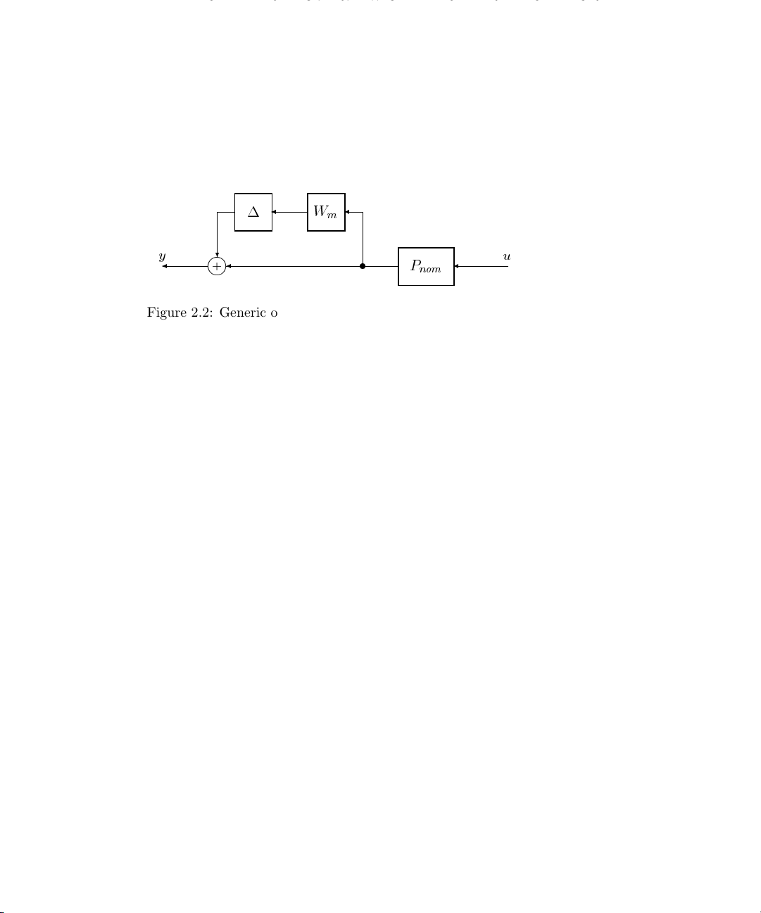
For example, consider the “uncertain” model illustrated in Figure 2.2. This picture is
equivalent to the input-output relationship,

y =[(I+∆W

y

  

m)Pnom

] u. (2.2)



W

m

s

P

nom

u

+

?

m



Figure 2.2: Generic output multiplicative perturbation model

In this figure, ∆, W

m

and P

theory can be stated with these blocks as elements of H

are dynamic systems. The most general form for the

nom

. For the purposes of

∞

calculation we will be dealing with Xmath Dynamic Systems, and in keeping with this
we will tend to restrict the theoretical discussion to RH

, stable, proper real rational

∞

transfer function matrices.

The only thing that we know about the perturbation, ∆, is that k∆k
with k∆k

≤ 1 gives a different transfer function between u and y. The set of all

∞

≤ 1. Each ∆,

∞

possible transfer functions, generated in this manner, is called P. More formally,





k∆k

P =(I +∆W

m)Pnom



≤ 1. (2.3)

∞

Now we are looking at a set of possible transfer functions,

y(s)=P(s)u(s),

where P (s) ∈P.

Equation 2.2 represents what is known as a multiplicative output perturbation
structure. This is perhaps one of the easiest to look at initially as W (s) can be viewed

2.2. MODELING UNCERTAIN SYSTEMS 15

as specifying a maximum percentage error between P
The system P

(s) is the element of P that comes from ∆ = 0 and is called the

nom

and every other element of P.

nom

nominal system. In otherwords, for ∆ = 0, the input-output relationship is
y(s)=P
nominal system is multiplied by (I +∆W

(s) u(s). As ∆ deviates from zero (but remains bounded in size), the

nom

(s)). Wm(s) is a frequency weighting function

m

which allows us the specify the maximum effect of the perturbation for each frequency.
Including W
normalization of ∆ is simply included in W

(s) allows us to model P with ∆ being bounded by one. Any

m

(s).

m

We often assume that ∆ is also linear and time-invariant. This means that ∆(ω)is
simply an unknown, complex valued matrix at each frequency, ω.Ifk∆k
each frequency, σ

(∆(ω)) ≤ 1. Section 2.2.3 gives a further discussion on the pros

max

≤1, then, at

∞

and cons of considering ∆ to be linear, time-invariant.

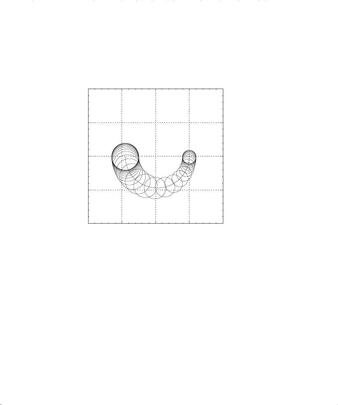
Now consider an example of this approach from a Nyquist point of view. A simple first
order SISO system with multiplicative output uncertainty is modeled as

y(s)=(I+W

(s)∆)P

m

nom

(s)u(s),

where

P

nom

(s)=

1+0.05s

1+s

and W

m

(s)=

0.1+0.2s
1+0.05s

.

Figure 2.3 illustrates the set of systems generated by a linear time-invariant ∆,

k∆k

≤ 1.

∞

At each frequency, ω, the transfer function of every element of P, lies within a circle,
centered at P

(ω), of radius |P

nom

(ω)Wm(ω)|. Note that for certain frequencies the

nom

disks enclose the origin. This allows us to consider perturbed systems that are
non-minimum phase even though the nominal system is not.

It is worth pointing out that P is still a model; in this case a set of regions in the
Nyquist plane. This is model set is now able to describe a larger set of system behaviors
than a single nominal model. There is still an inevitable mismatch between any model
(robust control model set or otherwise) and the behaviors of a physical system.

16 CHAPTER 2. OVERVIEW OF THE UNDERLYING THEORY

1

0.5

0

Imaginary

-0.5

-1
0 0.5 1-0.5 1.5

Real

Figure 2.3: Nyquist diagram of the set of systems, P

2.2. MODELING UNCERTAIN SYSTEMS 17





W

a

y



?

j

u u j



+

P

0

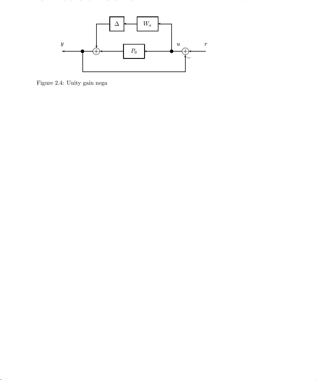
Figure 2.4: Unity gain negative feedback for the example system, P0+∆W

u r



+

,

6

a

2.2.2 Linear Fractional Transformations

A model is considered to be an interconnection of lumped components and perturbation
blocks. In this discussion we will denote the input to the model by u, which can be a
vector valued signal representing input signals such as control inputs, disturbances, and
noise. The outputs signal, denoted in this discussion by y, are also vector valued and can
represent system outputs and other variables of interest.

In order to treat large systems of interconnected components, it is necessary to use a
model formulation that is general enough to handle interconnections of systems. To
illustrate this point consider an affine model description:

y =(P

where u is the input and y is the output. ∆ again represents an unknown but bounded
perturbation. This form of perturbed model is known as an additive perturbation
description. While such a description could be applied to a large class of linear systems,
it is not general enough to describe the interconnection of models. More specifically, an
interconnection of affine models is not necessarily affine. To see this, consider unity gain
positive feedback around the above system. This is illustrated in Figure 2.4.

+∆Wa)u, k∆k∞≤ 1, (2.4)

0

The new input-output transfer function is

y =(P

+∆Wa)[I +(P0+∆Wa)]−1r. (2.5)

0

It is not possible to represent the new system with an affine model. Note that stability
questions arise from the consideration of the invertibility of [I +(P

+∆Wa)].

0

18 CHAPTER 2. OVERVIEW OF THE UNDERLYING THEORY



1

-

z v

.

.

.



m

P

11

 

y

P

21

P

P

12

22



u

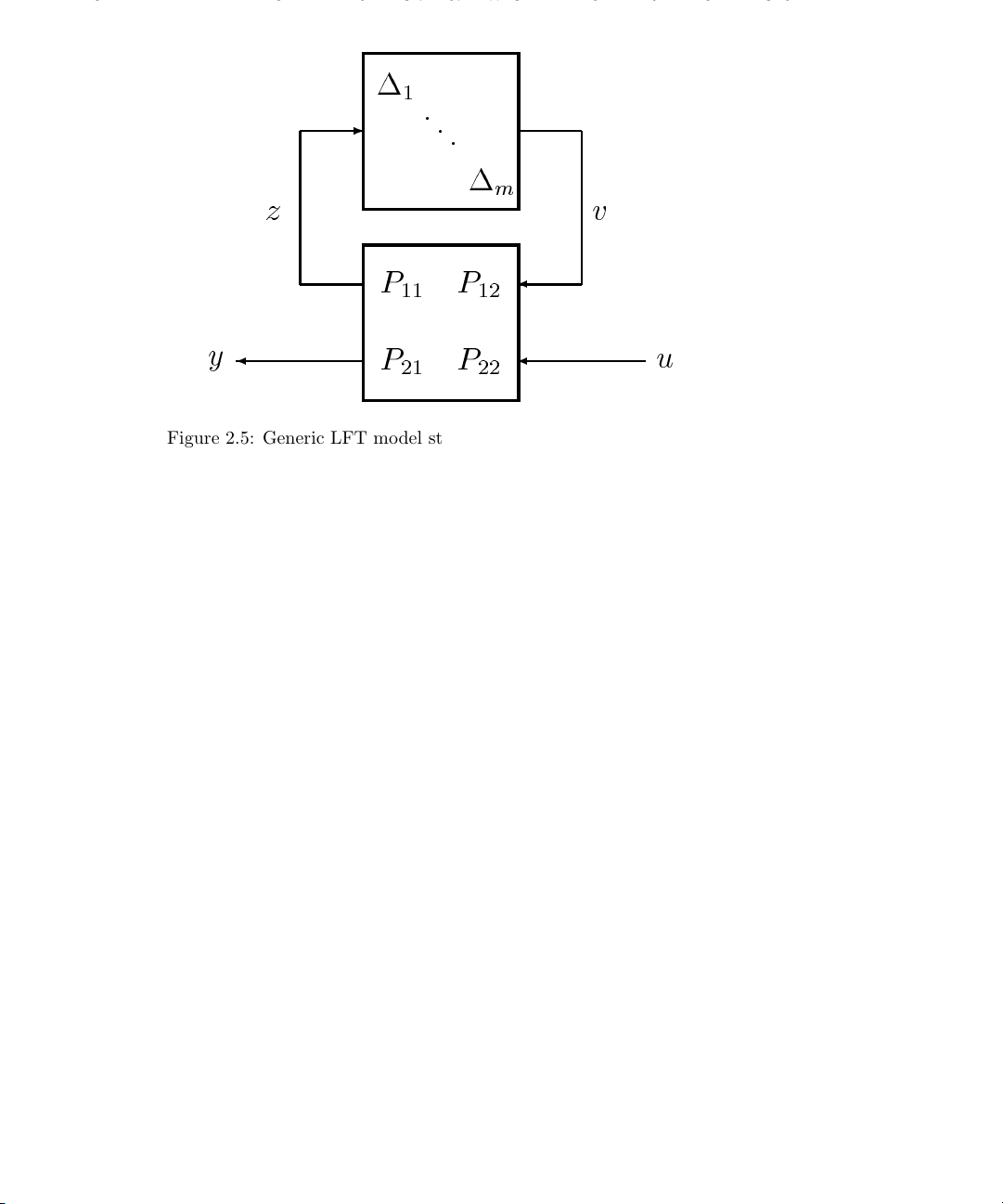
Figure 2.5: Generic LFT model structure including perturbations,∆

A generic model structure, referred to as a linear fractional transformation (LFT),
overcomes the difficulties outlined above. The LFT model is equivalent to the
relationship,



y =P

∆(I − P11∆)−1P12+ P

21

u, (2.6)

22

where the ∆ is the norm bounded perturbation. Figure 2.5 shows a block diagram
equivalent to the system described by Equation 2.6. Because this form of interconnection
is widely used, we will give it a specific notation. Equation 2.6 is abbreviated to,

y = F

(P, ∆)u.

u

The subscript, u, indicates that the ∆ is closed in the upper loop. We will also use

(., .) when the lower loop is closed.

F

l

In this figure, the signals, u, y, z and v can all be vector valued, meaning that the
partitioned parts of P ,(P

, etc.) can themselves be matrices of transfer functions.

11

To make this clear we will look at the perturbed system example, given in Equation 2.4,

2.2. MODELING UNCERTAIN SYSTEMS 19

in an LFT format. The open-loop system is described by,

u(Polp

, ∆)u,

y = F

where

0 W

IP

0



a

.



=

P

olp

The unity gain, negative feedback configuration, illustrated in Figure 2.4 (and given in
Equation 2.5) can be described by,

u(Gclp

, ∆)r,

y = F

where



(I + P0)−1Wa(I + P0)

−W

=

G

clp

a

(I + P0)

−1

P0(I + P0)

−1

−1



Figure 2.5 also shows the perturbation, ∆ as block structured. In otherwords,

∆ = diag(∆

,...,∆m). (2.7)

1

This allows us to consider different perturbation blocks in a complex interconnected
system. If we interconnect two systems, each with a ∆ perturbation, then the result can
always be expressed as an LFT with a single, structured perturbation. This is a very
general formulation as we can always rearrange the inputs and outputs of P to make ∆
block diagonal.

The distinction between perturbations and noise in the model can be seen from both
Equation 2.6 and Figure 2.5. Additive noise will enter the model as a component of u.
The ∆ block represents the unknown but bounded perturbations. It is possible that for
some ∆, (I − P

∆) is not invertible. This type of model can describe nominally stable

11

systems which can be destabilized by perturbations. Attributing unmodeled effects
purely to additive noise will not have this characteristic.

20 CHAPTER 2. OVERVIEW OF THE UNDERLYING THEORY

The issue of the invertibility of (I − P

∆) is fundamental to the study of the stability of

11

a system under perturbations. We will return to this question in much more detail in
Section 2.4. It forms the basis of the µ analysis approach.

Note that Equation 2.7 indicates that we have m blocks, ∆

, in our model. For

i

notational purposes we will assume that each of these blocks is square. This is actually
without loss of generality as in all of the analysis we will do here we can square up P by
adding rows or columns of zeros. This squaring up will not affect any of the analysis
results. The software actually deals with the non-square ∆ case; we must
specify the input and output dimensions of each block.

The block structure is a m-tuple of integers, (k

block. It is convenient to define a set, denoted here by ∆, with the appropriate block

∆

i

,...,km), giving the dimensions of each

1

structure representing all possible ∆ blocks, consistent with that described above. By
this it is meant that each member of the set of ∆ be of the appropriate type (complex
matrices, real matrices, or operators, for example) and have the appropriate dimensions.
In Figure 2.5 the elements P

. For consistency the sum of the column dimensions of the ∆imust equal the row

∆

i

dimension of P

∆ =ndiag (∆

. Now define ∆ as

11

,...,∆m)

1

It is assumed that each ∆
norm bound is one. If the input to ∆

and P12are not shown partitioned with respect to the

11




dim(∆i)=ki×k



is norm bounded. Scaling P allows the assumption that the

i

is ziand the output is vi,then

i

o

.

i

k = k∆izik≤kzik.

kv

i

It will be convenient to denote the unit ball of ∆, the subset of ∆ norm bounded by
one, by B∆. More formally



B∆ =n∆ ∈ ∆



k∆k≤1o.



Putting all of this together gives the following abbreviated representation of the
perturbed model,

y = F

(P,∆)u, ∆ ∈ B∆. (2.8)

u

2.2. MODELING UNCERTAIN SYSTEMS 21

w

?

W

n



W



u

y

+

?

j

?

j



+

u

P

nom

u



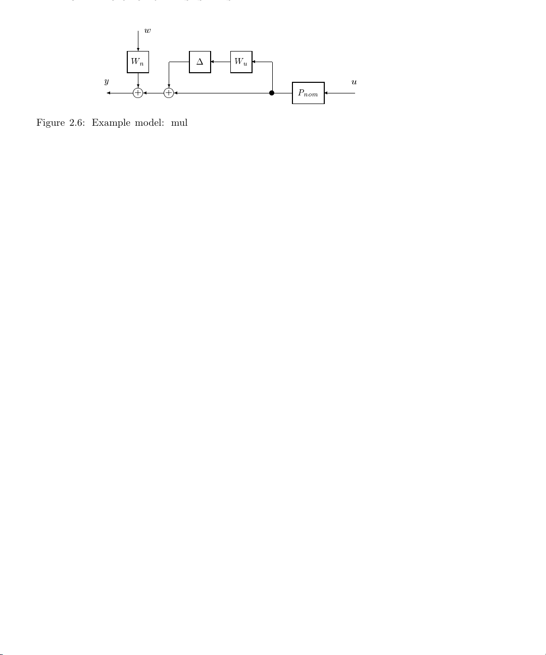
Figure 2.6: Example model: multiplicative output perturbation with weighted output
noise

References to a robust control model will imply a description of the form given in
Equation 2.8.

As a example, consider one of the most common perturbation model descriptions,
illustrated in Figure 2.6. This model represents a perturbed system with bounded noise
at the output.

The example model is given by,

y = W

n

The system W

w +(I+∆Wu)P

is a frequency dependent weight on the noise signal, w. This allows us

n

nom

u.

to use a normalized representation for w. In other words the model includes the
assumption that kwk

≤ 1. Similarly, we assume that k∆k∞≤ 1andWuis a frequency

∞

dependent weight which specifies the contribution of the perturbation at each frequency.
In a typical model W
nominal output) and W

will be small (assuming that the noise is small compared to the

n

will increase at high frequencies (to capture the likely case that

u

we know less about the model at higher frequencies). The LFT representation of this
model is,

where

y = F

P =

h

i

(P, ∆)

u

w

,

u

"

00W

IW

n

P

P

u

nom

nom

#

22 CHAPTER 2. OVERVIEW OF THE UNDERLYING THEORY

Robust control models are therefore set descriptions. In the analysis of such models it is
also assumed that the unknown inputs belong to some bounded set. Several choices of
set for the unknown signals can be made, leading to different mathematical problems for
the analysis. Unfortunately not all of them are tractable. The following section discusses
the assumptions typically applied to the robust control models.

2.2.3 Assumptions on P , ∆, and the unknown signals

It will be assumed that the elements of P are either real-rational transfer function
matrices or complex valued matrices. The second case arises in the frequency by
frequency analysis of systems.

In modeling a system, P

defines the nominal model. Input/output effects not

22

described by the nominal model can be attributed to either unknown signals which are
components of the model input (w in the previous example), or the perturbation ∆.
Unmodeled effects which can destabilize a system should be accounted for in ∆. The ∆
can loosely be considered as accounting for the following. This list is by no means
definitive and is only included to illustrate some of the physical effects better suited to
description with ∆.

• Unmodeled dynamics. Certain dynamics may be difficult to identify and there

comes a point when further identification does not yield significant design
performance improvement.

• Known dynamics which have been bounded and included in ∆ to simplify the

model. As the controller complexity depends on the order of the nominal model a
designer may not wish to explicitly include all of the known dynamics.

• Parameter variations in a differential equation model. For example linearization

constants which can vary over operating ranges.

• Nonlinear or inconsistent effects. At some point a linear model will no longer

account for the residual differences between the behaviors of the model and the
physical system.

Several assumptions on ∆ are possible. In the most general case ∆ is a bounded
operator. Alternatively ∆ can be considered as a linear time varying multiplier. This
assumption can be used to capture nonlinear effects which shift energy between
frequencies. Analysis and synthesis are possible with this assumption; Doyle and

2.2. MODELING UNCERTAIN SYSTEMS 23

Packard [19] discuss the implications of this assumption on robust control theory and we
briefly touch upon this in Section 2.4.6. The most common assumption is that ∆ is an
unknown, norm-bounded, linear time-invariant system.

Systems often do not fall neatly into one of the usual choices of ∆ discussed above.
Consider a nonlinear system linearized about an operating point. If a range of operation
is desired then the linearization constants can be considered to lie within an interval.
The model will have a ∆ block representing the variation in the linearization constants.
If this is considered to be a fixed function of frequency then the model can be considered
to be applicable for small changes about any operating point in the range. The precise
meaning of small will depend on the effect of the other ∆ blocks in the problem.

If the ∆ block is assumed to be time-varying then arbitrary variation is allowed in the
operating point. However this variation is now arbitrarily fast, and the model set now
contains elements which will not realistically correspond to any observed behavior in the
physical system.

The robust control synthesis theory gives controllers designed to minimize the maximum
error over all possible elements in the model set. Including non-physically motivated
signals or conditions can lead to a conservative design as it may be these signals or
conditions that determine the worst case error and consequently the controller.
Therefore the designer wants a model which describes all physical behaviors of the
system but does not include any extraneous elements.

The designer must select the assumptions on P and ∆. An inevitable tradeoff arises
between the ideal assumptions given the physical considerations of the system, and those
for which good synthesis techniques exist.

The most commonly used assumption is that ∆ is a linear time invariant system. This
allows us to consider the interconnection, F

(P, ∆), from a frequency domain point of

u

view. At each frequency ∆ can be taken as an unknown complex valued matrix of norm
less than or equal to one. This leads to analyses (covered in Section 2.4) involving the
complex structured singular value. The following section discusses more complicated
block structures and their use in modeling uncertain systems.

2.2.4 Additional Perturbation Structures

Equation 2.7 introduced a perturbation structure, ∆ containing m perturbation blocks,

. This form of perturbation is applicable to a wide range of models for uncertain

∆

i

24 CHAPTER 2. OVERVIEW OF THE UNDERLYING THEORY

systems. We will now look at other possible perturbation structures. For more detail on
these structures (in the complex case) refer to Packard and Doyle [20].

Consider a blocks which are of the form scalar × identity, where the scalar is unknown.
In the following we will include q of these blocks in ∆. The definition of ∆ is therefore
modified to be,

∆ =ndiag(δ

,...,δqIq,∆1,...,∆m)

1I1




dim(Ij)=lj×lj,dim(∆i)=ki×k



i

o

.(2.9)

The block structure now contains the dimension of the q scalar × identity blocks and the

m full blocks. The block structure is therefore, (l

,...,lq,k1,...,km). If

1

dim(∆) = n × n, then these dimensions must be consistent. In otherwords,

q

X

j=1

lj+

m

X

i=1

ki= n.

Note that this block structure collapses to the previously defined structure
(Equation 2.7) when q =0.

The most obvious application of a repeated scalar block structure occurs when we know
that perturbations occurring in several places in a system are identical (or perhaps just
correlated). For example, dynamic models of aircraft often have the altitude (or
dynamic pressure) occuring in several places in the model. Naturally the same value
should be used in each place and if we model the altitude as an LFT parameter then the
repeated scalar × identity approach is the most appropriate.

This structure also allows us to express uncertain state-space models as LFTs. To
illustrate this consider the following discrete time system.

x(k +1) = Ax(k)+Bu(k)

y(k)=Cx(k)+Du(k).

This digital system has transfer function,

P (z)=C(zI − A)

−1

B + D

2.2. MODELING UNCERTAIN SYSTEMS 25

−1

= Cz

= F

(I − z−1A)−1B + D

,z−1I),

u(Pss

where P

and the scalar × identity, z

is the real valued matrix,

ss



=

P

ss

AB
CD



,

−1

I, has dimension equal to the state dimension of P (z).

This is now in the form of an LFT model with a single scalar × identity element in the
upper loop.

One possible use of this is suggested by the following. Define,



∆ =δI

nx



δ ∈C,

where nx is the state dimension. The set of models,

F

, ∆), ∆ ∈ B∆,

u(Pss

is equivalent to P (z), |z|≥1. This hints at using this formulation for a stability analysis
of P(z). This is investigated further in Section 2.4.6.

In the analyses discussed in Section 2.4 we will concentrate on the assumption that ∆ is
complex valued at each frequency. For some models we may wish to restrict ∆ further.
The most obvious restriction is that some (or all) of the ∆ blocks are real valued. This is
applicable to the modeling of systems with uncertain, real-valued, parameters. Such
models can arise from mathematical system models with unknown parameters.

Consider, for example a very simplified model of the combustion characteristics of an
automotive engine. This is a simplified version of the model given by Hamburg and
Shulman [21]. The system input to be considered is the air/fuel ratio at the carburettor.
The output is equivalent to the air/fuel ratio after combustion. This is measured by an
oxygen sensor in the exhaust. Naturally, this model is a strong function of the engine
speed, v (rpm). We model the relationship as,

y =e

−Tds



0.9

1+Tcs

+

0.1

1+s



u,

26 CHAPTER 2. OVERVIEW OF THE UNDERLYING THEORY

where the transport delay, T

252

v

and T

T

=

d

, and the combustion lag, Tc, are approximately,

d

202

.

=

c

v

For the purposes of our example we want to design an air/fuel ratio controller that
works for all engine speeds in the range 2,000 to 6,000 rpm. We will use a first order
Pad´e approximation for the delay and express the T
form with a normalized speed deviation, δ

.

v

The dominant combustion lag can be expressed as an LFT on 1/T

0.9

1+Tcs

= F

u(Ptc

,T

−1

c

),

and Tcrelationships in an LFT

d

as follows,

c

where

P

=

tc

Note that T



−1



0.9

−1

is easily modeled in terms of δv,

c



1

s



.

0

s

4000 + 2000δ

1

=

T

c

202

v

,δ

∈R, |δv|≤1.

v

The Pad´e approximation (with delay time, T

−Tds

e

≈F



P

u

delay

,T

d

−1



,

where,

P

delay



−2

s



=

4

s

1

−1





.

)isgivenby

d

2.2. MODELING UNCERTAIN SYSTEMS 27

Putting all the pieces together gives an engine model in the following fractional form.

P (s)=F

u(Pmod

, ∆),

where

P

mod

=










−15.87

s

0

−27.75

s

7.14(s − 19.8)

2

s

−9.9

s

−0.9(s − 15.8)(s − 19.8)

3

s

141.5(1 + 1.006s)
s(s +1)

9.9

−17.82(s − 15.8)(1 + 1.006s)

s(s +1)

and ∆ ∈ B∆, with the structure defined as,



∆ =δ

vI2



δ

∈R.

v

To capture the effects of unmodeled high frequency dynamics we will also include an
output multiplicative perturbation. If the output multiplicative weight is W

(s)then

m

the complete open-loop model is,

P (s)=F

u(Pmod

, ∆), (2.10)










,

where,

P

mod



−15.87

s






0




=



−27.75



s





−27.75

s

7.14(s − 19.8)

2

s

−9.9

s

−0.9(s − 15.8)(s − 19.8)

3

s

−0.9(s − 15.8)(s − 19.8)

3

s

0

09.9

0

Wm(s)

141.5(1 + 1.006s)
s(s +1)

−17.82(s − 15.8)(1 + 1.006s)

s(s +1)

−17.82(s − 15.8)(1 + 1.006s)

s(s +1)















28 CHAPTER 2. OVERVIEW OF THE UNDERLYING THEORY

and ∆ ∈ B∆, with the structure defined as,





, ∆1)

∆ =diag(δ

vI2

δv∈R,∆1∈C.



Note that this is an LFT with a repeated real-valued parameter, δ
complex perturbation, ∆

Note that as R⊂C, assuming that ∆ ∈C
∆

(or δj) are more appropriately modeled as real-valued. However this may be

i

potentially conservative as the ∆ ∈C

(|∆1|≤1).

1

n×n

, always covers the case where some of the

n×n

, allows many more systems in the model set.

In this case it would be somewhat better to consider combining the effects of δ

(|δv|≤1), and a

v

v

and ∆

into a single complex valued ∆ with an appropriate weight.

In principle, if we have additional information about the system (some δ

∈R,for

j

example) then we should use this information. Performing analyses with real valued
perturbations is currently at the forefront of the structured singular value research. We
will return to this issue in more detail when we cover the analysis methods (Section 2.4).

2.2.5 Obtaining Robust Control Models for Physical Systems

Obtaining a model of the above form is where the real engineering comes in. A designer
must model and identify the physical system to arrive at such a model. This is usually
an iterative process whereby designs are performed and then tested on the system. In
this way the designer often obtains a feeling for the adequacy of the model.

The best way of studying the modeling problem is to look at the documented
experiences of others applying these approaches; particularly in similar applications. The
citations given in the Section 2.1 will be useful in this regard. There are also approaches
addressing the problem of obtaining LFT models from descriptions with variable
state-space matrix coefficients [22, 23]. In the area of SISO process control, Laughlin et
al. [24] describe the relationship between uncertainties in time constant, delay, and gain,
and a suitable ∆ weighting. Models of this form are often applicable to process control.

1

There is little formal theory addressing the robust control modeling problem although
this is an area of increasing interest. A recent workshop proceedings volume on the
subject is an excellent reference for those interested in this area [25]. Other references
can be found in the review article by Gevers [26].

2.3. H∞AND H2DESIGN METHODOLOGIES 29

An area of work, known as identification in H
techniques which minimize the worst case H

, looks at experimental identification

∞

error between the physical system and

∞

the model. The following works address this issue: [27, 28, 29, 30, 31, 32, 33, 34, 35].

Applying the more standard, probabilistically based, identification techniques to
uncertain systems is also receiving attention. Relevant work in this area is described
in: [36, 37, 38, 39]

Model validation is the experimental testing of a given robust control model. This can
be useful is assessing model quality. This work is covered in the
following: [4, 40, 41, 42, 43, 44, 45, 46]. An experimental example is described by
Smith [47].

The problems of identifying model parameters in an uncertain model is discussed further
in [48, 49, 50]. A nonlinear ad-hoc approach for obtaining suitable multiplicative
perturbation models for certain classes of systems is given in [51].

Several researchers are also formalizing the interplay between identification and design
in iterative approaches. In practical situations the designer usually ends up with ad-hoc
identification/design iterations. The work in this area is described in [52, 53, 54, 55, 56].

On reading the above works, one will get the impression that this area is the most
poorly developed of the current robust control theory. In obtaining these models
engineering judgement is of paramount importance. The users of this software are
encouraged to document their experiences and bring this work to the authors’ attention.

2.3 H∞and H2Design Methodologies

The generic synthesis configuration is illustrated in LFT form in Figure 2.7. Here P (s)
is referred to as the interconnection structure. The objective is to design K(s) such that
the closed loop interconnection is stable and the resulting transfer function from w to e
(denoted by G(s)),

e = F

satisfies a norm objective.

[P (s),K(s)]w,

l

= G(s)w,

30 CHAPTER 2. OVERVIEW OF THE UNDERLYING THEORY

e w

 

P(s

)



y

-

K(s

)

u

Figure 2.7: LFT configuration for controller synthesis, G(s)=Fl[P(s),K(s)]

Note that the interconnection structure, P (s), given here, differs from that discussed in
the previous section. Here we set up P (s) so that the input, w, is the unknown signals
entering our system. Typical examples would be sensor noise, plant disturbances or
tracking commands. The output, e, represent signals that we would like to make small.
In an engineering application these could include actuator signals and tracking errors.

The signal y is the measurement available to the controller, K(s). In any realistic
problem, some weighted component of w would be added to y to model sensor noise.
The output of the controller, u, is our actuation input to the system. Again, a
reasonable engineering problem would include a weighted u signal as a component of the
penalty output, e.

The interconnection structure, P(s), also contains any frequency weightings on the
signals e and w. Weightings on components of e are used to determine the relative
importance of the various error signals. Weight functions on w indicate the relative
expected size of the unknown inputs.

Xµ provides functions to calculate the controllers minimizing either the H

or H∞norm

2

of G(s). We will cover both of these approaches in the context of the design problem
illustrated in Figure 2.7.

Note that neither of these design approaches takes advantage of any information about
structured perturbations occuring within the model. The following discussion can be
considered as applying to a nominal design problem. Section 2.5 uses D-K iteration to

2.3. H∞AND H2DESIGN METHODOLOGIES 31

extend these approaches to the case where P (s) is replaced by F

(P (s), ∆), ∆ ∈ B∆.

u

2.3.1 H∞Design Overview

Again, recall from Section 2.1.2, the H∞is norm of G(s)is,

=supωσ

∞

norm is the induced L2to L2norm. Therefore minimizing the H∞norm of

The H

kG(s)k

∞

G(s) will have the effect of minimizing the worst-case energy of e over all bounded
energy inputs at w.

Consider γ(K ) to be the closed loop H
other words,

γ(K)=kF

(P, K)k∞.

l

There is a choice of controller, K, which minimizes γ(K ). This is often referred to as the
optimal value of γ and is denoted by γ
which satisfies,

max

[G(ω)].

norm achieved for a particular controller K.In

∞

. Furthermore, there is no stabilizing controller

opt

kG(s)k

∞<γopt

In a particular design problem, γ
calculating the H
to γ

.

opt

.

is not known a priori. Therefore the functions

opt

controller use some form of optimization to obtain a value of γ close

∞

The first approaches to the solution of this problem were described by Doyle [1]. The
book by Francis [57] gives a good overview of the early version of this theory. A
significant breakthrough was achieved with the development of state-space calculation
techniques for the problem. These are discussed in the paper colloquially known as
DGKF [58]. The algorithmic details are actually given by Glover and Doyle [59].

32 CHAPTER 2. OVERVIEW OF THE UNDERLYING THEORY

2.3.2 Assumptions for the H∞Design Problem

There are several assumptions required in order to achieve a well-posed design problem.
The DGKF paper gives a state-space solution to the H
a similar notation here.

Consider the open loop state-space representation of P (s), partitioned according to the
signals shown in Figure 2.7,

design problem and we will use

∞

P (s)=





A
C
C

1

2

B1B
D11D
D21D



2



. (2.11)

12

22

We will assume that P (s) is a minimal representation. The following assumptions are
required for a well-posed problem.

(i)(A, B

(ii) D

) is stabilizable and (C2,A) is detectable;

2

and D21are full rank;

12

(iii) The matrix,

D



2

,

12



A − ωI B

C

1

has full column rank for all ω ∈R;

(iv ) The matrix,

D



1

,

21



A − ωI B

C

2

has full row rank for all ω ∈R.

Item (i) is required so that input-output stability is equivalent to internal stability. If it
is not satisfied then there are unstable modes which cannot be stabilized by any K(s).

Items (ii)and(iii ) mean that, at every frequency, there is no component of the output
signal, e, that cannot be influenced by the controller. Similarly, items (ii)and(iv)mean

2.3. H∞AND H2DESIGN METHODOLOGIES 33

that the effect of all disturbances, w, at every frequency, can be measured by the
controller. If either of these conditions are not met then the problem could be ill-posed.

It is possible to violate these conditions by using pure integrators as design weights.
While this could still give a meaningful design problem, solution via the state-space H

∞

approach requires that an approximation be used for the integrator weight. If item (iii)
or (iv) is violated at ω = 0, then the integrator should be replaced with very low
frequency pole.

2.3.3 A Brief Review of the Algebraic Riccati Equation

Solution of the H∞design problem requires the solution of coupled Algebraic Riccati
Equations (AREs). This is illustrated in more detail in the next section. Here we give a
very brief review of the Riccati equation and the most common solution techniques.
Some knowledge of this area is helpful because the design software displays variables
related to the Riccati solutions and the user has the option of adjusting several software
tolerances relating to these solutions. The notation used here comes from DGKF [58].

The matrix equation,

T

A

X + XA +XRX − Q =0,

is an ARE. Given A, R and Q (with R and Q symmetric), we are interested in finding a

T

symmetric positive definite solution, X . In other words, X = X

≥ 0. With this ARE

we associate a Hamiltonian matrix, denoted by H,

H =



AR
Q−A

T



.

If dim(A)=n×n, then dim(H)=2n×2n. Assume that H has no ω axis eigenvalues.
The structure of H meansthatithasnstable (Re{s} < 0) and n unstable (Re{s} > 0)
eigenvalues.

Now consider finding a basis for the stable eigenvalues. Stacking the basis vectors
together will give a 2n × n matrix,

i

h

X

1

.

X

2

34 CHAPTER 2. OVERVIEW OF THE UNDERLYING THEORY

We have partitioned the matrix into two n × n blocks, X

and X2.IfX1is invertible,

1

then

−1

X

X = X

,

2

1

is the unique, stabilizing solution to the ARE. The ability to form X doesn’t depend on
the particular choice of X

and X2.

1

Given a Hamiltonian, H,wesaythatH∈dom(Ric) if H has no ω axis eigenvalues and
the associated X

matrix is invertible. Therefore, if H ∈ dom(Ric), we can obtain a

1

unique stabilizing solution, X. This mapping, from H to X , is often written as the
function, X = Ric(H).

To give an idea of the application of the ARE consider the following lemma (taken from
DGKF).

Lemma 1 Suppose H ∈ dom(Ric) and X = Ric(H). Then:

a) X is symmetric;

b) X satisfies the ARE,

T

A

X + XA +XRX − Q =0;

c) A + RX is stable.

This is of course the well know result relating AREs to the solution of stabilizing state
feedback controllers.

AREs can also be used in calculating the H

-norm of a state-space system. The

∞

approach outlined here is actually that used in the software for the calculation of
kP (s)k

. Consider a stable system,

∞



P (s)=

B

A
C 0



.

2.3. H∞AND H2DESIGN METHODOLOGIES 35

Choose γ>0 and form the following Hamiltonian matrix,



.

T

<γ.Aproofof

∞

H =



−CTC −A

−2BBT

Aγ

The following lemma gives a means of checking whether or not kP (s)k
this lemma is given in DGKF although it is based on the work of Anderson [60],
Willems [61] and Boyd et al.[62].

Lemma 2 The following conditions are equivalent:

a) kP (s)k

∞

<γ;

b) H has no eigenvalues on the ω axis;

c) H ∈ dom(Ric);

d) H ∈ dom(Ric) and Ric(H ) ≥ 0 (if (C,A) is observable then Ric(H) > 0).

As the above illustrates, AREs play a role in both stabilization and H
calculations for state-space systems. Before giving more detail on the H

-norm

∞

∞

design
problem (Section 2.3.4), we will discuss some of the issues that arise in the practical
calculation of ARE solutions.

We can summarize an ARE solution method as follows:

(i) Form the Hamiltonian, H.

(ii)CheckthatHhas no ω axis eigenvalues.

(iii) Find a basis for the stable subspace of H.

(iv)CheckthatX

(v) Form X = X

is invertible.

1

−1

X

.

2

1

The first issue to note is that it is difficult to numerically determine whether or not H
has ω axis eigenvalues. A numerical calculation of the eigenvalues is unlikely to give

36 CHAPTER 2. OVERVIEW OF THE UNDERLYING THEORY

any with a zero real part. In practice we must use a tolerance to determine what is
considered as a zero real part.

Finding a basis for the stable subspace of H involves either an eigenvalue or Schur
decomposition. Numerical errors will be introduced at this stage. In most cases using an
eigenvalue decomposition is faster and less accurate than using a Schur decomposition.
Similarly, forming X = X

−1

X

will also introduce numerical errors. The Schur solution

2

1

approach, developed by Laub et al. [63, 64, 65], is currently the best numerical approach
to solving the ARE and is used in the software as the default method. An overview of
invariant subspace methods for ARE solution is given by Laub [66]. Accurate solution of
the ARE is still very much an active area of research.

2.3.4 Solving the H∞Design Problem for a Special Case

We will now look at the H∞design problem for a simplifying set of assumptions. The
general problem (with assumptions given in Section 2.3.2) can be transformed into the
simplified one given here via scalings and other transformations. The simplified problem
illustrates the nature of the solution procedure and is actually the problem studied in
DGKF. The formulae for the general problem are given in Glover and Doyle [59]. The
software solves the general problem.

Consider the following assumptions, with reference to the system in Equation 2.11:

(i)(A,B

(ii)(A,B

(iii) D

(iv)

(v) D

) stabilizable and (C1,A) detectable;

1

) stabilizable and (C2,A) detectable;

2

T

[ C1D12]=[0 I];

12



D21D

= D22=0.

11



h

B

1

T

21

i

0

=

;

I

Assumption (i) is included in DGKF for technical reasons. The formulae are still correct
if it is violated. Note that, with these assumptions,

e = C

x + D12u,

1

2.3. H∞AND H2DESIGN METHODOLOGIES 37

and the components, C

x and D12u are orthogonal. D12is also assumed to be

1

normalized. This essentially means that there is no cross-weighting between the state
and input penalties. Assumption (iv) is the dual of this; the input and unknown input
(disturbance and noise) affect the measurement, y, orthogonally, with the weight on the
unknown input being unity.

To solve the H

=

H

∞

design problem we define two Hamiltonian matrices,

∞



−C

T

C

−2

1

Aγ

1

T

B1B

−B2B

1

T

−A



T

2

,

and



=

A

−B1B

T

1

J

∞

T

γ−2C

T

C1− C

1

−A



T

C

2

2

.

The following theorem gives the solution to the problem.

Theorem 3 There exists a stabilizing controller satisfying kG(s)k

<γ if and only if

∞

the following three conditions are satisfied:

a) H

b) J

c) ρ(X

∈ dom(Ric) and X∞= Ric(H∞) ≥ 0.

∞

∈ dom(Ric) and Y∞= Ric(J∞) ≥ 0.

∞

) <γ2.

∞Y∞

When these conditions are satisfied, one such controller is,



,

0

K

(s)=

∞



ˆ

A

∞−Z∞L∞

F

∞

where,

F

∞

= −B

T

X

∞

2

38 CHAPTER 2. OVERVIEW OF THE UNDERLYING THEORY

= −Y∞C

L

∞

Z∞=(I−γ−2Y∞X∞)

ˆ

=A+γ−2B1B

A

∞

T

2

−1

T

X∞+B2F∞+Z∞L∞C2.

1

Actually, the above formulation can be used to parametrize all stabilizing controllers
which satisfy, kG(s)k

<γ. This can be expressed as an LFT. All such controllers are

∞

given by,

= Fl(M∞,Q),

K

∞

where,



ˆ

A

∞

M



=

∞

F

−C

∞

2

and Q satisfies: Q ∈RH

−Z∞L∞Z∞B

0 I
I 0

,kQk∞<γ.NotethatifQ= 0 we get back the controller

∞



2



,

given in Theorem 3. This controller is referred to as the central controller and it is the
controller calculated by the software.

Note also that the controller given above satisfies kGk
controller that minimizes kGk

and is therefore referred to as a suboptimal H

∞

<γ. It is not necessarily the

∞

∞

controller. In practice this is not a problem, and may even be an advantage. The optimal

H

controller has properties which may not be desirable from an implementation point

∞

of view. One typical property is that the high frequency gain is often large. Suboptimal
central controllers seem to be less likely to exhibit this characteristic.

2.3.5 Further Notes on the H∞Design Algorithm

Now that we have covered the problem solution we can look at the areas that might give
potential numerical problems. The above results give a means of calculating a controller
(if one exists) for a specified γ value. As we mentioned earlier, the smallest such γ is
referred to as γ

. An iterative algorithm is used to find γ close to γ

opt

the resulting controller. The algorithm can be stated conceptually as follows:

and calculate

opt

2.3. H∞AND H2DESIGN METHODOLOGIES 39

a) Choose γ ≥ γ

b) Form H∞and J

opt

∞

c) Check that H∞∈ dom(Ric) and J∞∈ dom(Ric).

d) Calculate X

e) Check that X

f) Check that ρ(X

= Ric(H∞)andY∞= Ric(J∞)

∞

≥ 0andY∞≥0

∞

2

) <γ

∞Y∞

g) Reduce γ andgotostepb).

The value of γ can be reduced until one of the checks at steps c), e) or f) fails. In this
case, γ<γ

and we use the X∞and Y∞of the lowest successful γ calculation to

opt

generate the controller. In the Xµ software a bisection search over γ is used to find a γ
close to γ

. If step a) is not satisfied, the routine exits immediately and tells the user

opt

to select a higher initial choice for γ.

As part of the check that H

∈ dom(Ric), (and J∞∈ dom(Ric)) the real part of the

∞

eigenvalues is calculated. The software uses a tolerance to determine whether or not to
consider these zero. The default tolerance works well in most cases; the user can adjust
it if necessary.

In practice determining that X

(and Y∞) is positive definite involves checking that,

∞

Re{λi(X∞)}≥−.

min

i

Again,  is a preset tolerance which can be adjusted by the user if necessary.

The third check is that,

−2

X∞Y∞) < 1.

ρ(γ

Fortunately this is a relatively well conditioned test.

The software displays the critical variables relating to each of these tests. The minimum
real part of the eigenvalues of H

(and J∞) is displayed. Similarly the minimum

∞

40 CHAPTER 2. OVERVIEW OF THE UNDERLYING THEORY

eigenvalue of X

(and Y∞) is displayed. The ultimate test of the software is to form the

∞

closed loop system and check both its stability and norm. We strongly suggest that the
user always perform this step.

The numerical issues discussed above are very unlikely to arise in low order systems.
Experience has shown that systems with very lightly damped modes are more
susceptible to numerical problems than those with more heavily damped modes.
However, it has been found to be possible, with the software provided, to design
controllers using 60th order interconnection structures with very lightly damped modes.

2.3.6 H2Design Overview

Recall from Section 2.1.2 that the H2norm of a frequency domain transfer function,
G(s), is



Z

∞

kG(s)k

1

=

2

2π

Trace [G(ω)∗G(ω)] dω

−∞

Several characterizations of this norm are possible in terms of input/output signals. For
example, if the unknown signals are of bounded energy, kGk
magnitude of the outputs e. Alternatively, if impulses are applied to the inputs of G(s),
kG(s)k
which minimizes the H

gives the energy of the outputs e. H2synthesis involves finding the controller

2

norm of the closed loop system. This is the same the well

2

studied Linear Quadratic Gaussian problem.



1/2

.

gives the worst case

2

2.3.7 Details of the H2Design Procedure

The H2design procedure is best explained by contrasting it with the H∞procedure
explained in the previous sections. There are several differences, the most obvious being
that the H
difference is that (in addition to the four conditions given in Section 2.3.2) D
required to be zero, even in the general case. If this condition is violated no controller
will give a finite H
frequency goes to ∞.

We present the H

design problem always has a unique, minimizing, solution. The other

2

norm for the closed loop system as it will not roll off as the

2

solution in an LFT framework rather than the more well known LQG

2

is

11

2.3. H∞AND H2DESIGN METHODOLOGIES 41

framework. We again assume the simplifying assumptions used in Section 2.3.4 The H
design solution is obtained (at least conceptually) from the H∞design procedure by
setting γ = ∞ and using the resulting central controller. It is interesting to compare the

H

solution, given above, and the H2solution given below.

∞

Define two Hamiltonians, H



H

=

2

A −B

T

−C

C1−A

1

and J2,by,

2



T

B

2

2

,

T

and



T

−C

=

J

2

A

−B1B

T

1

The sign definiteness of the off-diagonal blocks guarantees that H

∈ dom(Ric) and X2= Ric(H2) ≥ 0andY2= Ric(J2) ≥ 0. The following theorem

J

2

T

2

−A



C

2

.

∈ dom(Ric),

2

gives the required result.

Theorem 4 The unique H



ˆ

A

K

(s)=

2

2−L2

F20

optimal controller is given by,

2



,

2

where,

= −B

F

2

L2= −Y2C

ˆ

= A + B2F2+ L2C2.

A

2

We commented above that the controller, K
γ = ∞ in the H
means that we can make no a priori prediction about kGk

T

X

2

2

T

2

, is (conceptually) obtained by choosing

2

design procedure. This does not mean that kGk∞= ∞; it simply

∞

for this controller. K

∞

2

minimizes kGk2and yields a finite kGk∞. As such, it is often useful for determining an

42 CHAPTER 2. OVERVIEW OF THE UNDERLYING THEORY

G(s

)

e w

 

P(s

-

)

K(s



)

Figure 2.8: Closed loop system, G(s), for performance analysis

initial choice of γ for the H
can also be used to initialize the D-K iteration procedure when an open-loop H

design procedure. We will see later (Section 2.5) that it

∞

∞

design

is poorly conditioned.

2.4 µ Analysis

2.4.1 Measures of Performance

Section 2.3 presented design performance objectives in terms of the norm (H2or H∞)of
a closed loop system. We will now expand on this idea of performance. Consider the
closed loop system illustrated in Figure 2.8. The interconnection structure, P (s), is
specified such that w represents unknown inputs; typically reference commands,
disturbances and noise. The outputs, e, represent signals that we would like to be small.
“Small” means in the sense of a selected norm. These signals might include actuator
effort, and tracking error. As Figure 2.8 suggests, this analysis is typically applied after
calculating a controller.

The inputs w are described only as members of a set. The performance question is then:
For al l w in this set, are all possible outputs e also in some set? The following set

2.4. µ ANALYSIS 43

descriptions are considered, where B again denotes the unit ball.

)

(2.12)

)

(2.13)

)

(2.14)

Power : BP =

Energy : BL

Magnitude : BL

=(w

2

=(w

∞

(





w

lim



T →∞





kwk







kwk∞= ess supt|w(t)|≤1



Z

T

1

2T

2

=

2

| w(t) |2dt ≤ 1

−T

Z

∞

| w(t) |2dt ≤ 1

−∞

These norms are defined for scalar signals for clarity. The choice of w and e as the above
sets defines the performance criterion. The performance can be considered as a test on
the corresponding induced norm of the system. More formally,

Lemma 5 (Nominal Performance)

For al l w in the input set, e is in the output set

if and only if kG(s)k≤1.

Only certain combinations of input and output sets lead to meaningful induced norms.
The H

/µ approach is based on the cases w, e ∈ BP and w, e ∈ BL2.Aswenotedin

∞

Section 2.1.2, both of these cases lead to the following induced norm.

kG(s)k

=supωσ

∞

max

[G(ω)] .

The choice of other input and output sets can lead to meaningful norms with
engineering significance. For example w, e ∈ BL
some problems and leads to kGk

Z

∞

=

kGk

1

|g(τ)| dτ.

0

as a performance measure where

1

is arguably a more suitable choice for

∞

and g(τ) is the convolution kernel (impulse response) of G(s). For a discussion on the
other possible selections of input and output sets, and the mathematical advantages of

44 CHAPTER 2. OVERVIEW OF THE UNDERLYING THEORY



1

-

z v

.

.

.



m

G

 

e w

G

11

21

G

G

12

22



Figure 2.9: Perturbed closed loop system for stability analysis

the induced norms, the reader is referred to Doyle [2]. The major advantage of choosing
BP or BL

is that the test for the performance can be considered in terms of the same

2

norm as stability. This has significant advantages when we are considering performance
and stability in the presence of perturbations, ∆.

2.4.2 Robust Stability and µ

Now we will consider the stability of a closed loop system under perturbations. In
Figure 2.9, G(s), is a perturbation model of a closed loop system. In the following
robust stability and robust performance analyses we will assume that ∆ is linear and
time-invariant.

We will also assume that the interconnection structure G(s) consists of stable transfer
function matrices, where stability is taken to mean that the system has no poles in the
closed right half plane. In practice this amounts to assuming that G
closed loop system model) is stable as the other elements, G

(s), G12(s), and G21(s),

11

are weighting functions and can be chosen to be stable. The nominal closed loop system,

(s), often arises from a standard design procedure (H2, H∞, or loopshaping for

G

22

example) and will be stable.

(s) (the nominal

22

2.4. µ ANALYSIS 45

Consider the case where the model has only one full ∆ block (m =1andq=0in
Equation 2.9). This is often referred to as unstructured, and the well known result (refer
to Zames [67] and Doyle and Stein [5]) is given in the following lemma.

Lemma 6 (Robust Stability, Unstructured)

(G(s),∆) is stable for all ∆, k∆k∞≤ 1,

F

u

if and only if kG

A generalization of the above is required in order to handle F

(s)k∞< 1.

11

(G(s), ∆) models with

u

more than one full ∆ block. The positive real valued function µ canbedefinedona
complex valued matrix M,by

det(I − M ∆) 6=0 forall∆∈B∆, if and only if µ(M) < 1.

Note that µ scales linearly. In other words, for all α ∈R,

µ(αM )=|α|µ(M).

In practice the test is normalized to one with the scaling being absorbed into the
interconnection structure. An alternative definition of µ is the following.




0ifno∆∈∆solves det(I + M ∆) = 0







µ(M)=

otherwise











∆∈∆

min



n



β

∃∆, k∆k≤β, such that det(I + M∆) = 0





−1

o

Note that µ is defined as the inverse of the size of the smallest destabilizing
perturbation. This immediately gives the following lemma.

Lemma 7 (Robust Stability, Structured)

46 CHAPTER 2. OVERVIEW OF THE UNDERLYING THEORY

(G(s), ∆) stable for all ∆ ∈ B∆

F

u

if and only if kµ(G

(s))k∞< 1.

11

where

kµ(G

(s))k∞=supωµ[G11(ω)].

11

The use of this notation masks the fact that µ is also a function of the perturbation
structure, ∆. The above definition of µ applies to the more general block structure given
in Section 2.2.4. We can even consider the some of the blocks to be real valued, rather
than complex valued. The robust stability lemma is still valid; however the calculation
of µ becomes significantly more difficult.

In applying the matrix definition of µ to a real-rational G

(s), it has been assumed that

11

∆ is a complex constant at each frequency. This arises from the assumption that ∆ is
linear and time-invariant. Under this assumption we can examine the combination of
system and perturbation independently at each frequency. The analysis then involves
looking for the worst case frequency. If ∆ is not time-invariant then the frequency by
frequency analysis does not apply; ∆ can be used to shift energy between frequencies
and cause instability not predicted by the above analysis.

In practice this µ test is applied by selecting a frequency grid and at each frequency
calculating µ(G

(ω)). The choice of range and resolution for this grid is a matter of

11

engineering judgement. If very lightly damped modes are present a fine grid may be
required in the region of those modes.

2.4.3 Robust Performance

The obvious extension to the above is to consider performance in the presence of
perturbations ∆. For e, w ∈ BP or BL
robust stability.

Lemma 8 (Robust Performance)

F

(G(s), ∆) is stable and kFu(G(s), ∆)k∞≤ 1 for all ∆ ∈ B∆

u

robust performance is a simple extension of

2

2.4. µ ANALYSIS 47

if and only if kµ(G(s))k

< 1,

∞

where µ is taken with respect to an augmented structureb∆,

b

∆ =ndiag(∆,ˆ∆)




∆ ∈ ∆,ˆ∆=C



dim(w)×dim(e)

o

.

The additional perturbation block,ˆ∆ can be thought of as a “performance block”
appended to the ∆ blocks used to model system uncertainty. This result is the major
benefit of the choice of input and output signal norms; the norm test for performance is
the same as that for stability. Robust performance is simply another µ test with one
additional full block.

The frequency domain robustness approach, outlined above, assumes that the
perturbations, ∆, are linear and time-invariant. This assumption is the most commonly
applied. Section 2.4.6 will consider a robustness analysis from a state-space point of
view. This form of analysis applies to norm bounded non-linear or time varying
perturbations. We will first look more closely at the properties of µ, particularly as they
relate to its calculation.

2.4.4 Properties of µ

The results presented here are due to Doyle [68]. Fan and Tits [69, 70] have done
extensive work on algorithms for tightening the bounds on the calculation of µ.
Packard [3] has also worked on improvement of the bounds and the extension of these
results to the repeated block cases. The most comprehensive article on the complex
singular value is that by Packard and Doyle [20]. More detail is contained in the
technical report by Doyle et al. [71].

We will look at simple bounds on µ. The upper bound results are particularly important
as they will form the basis of the design procedure provided in this software (D-K
iteration).

Defining a block structure made up of one repeated scalar, (∆ = {λI | λ ∈C})makes
the definition of µ the same as that of the spectral radius.



∆ =nλI



λ ∈Co⇒ µ(M)=ρ(M).



48 CHAPTER 2. OVERVIEW OF THE UNDERLYING THEORY

n×n

For the other extreme consider a single full block (∆ = {∆ | ∆ ∈C

}); the definition

of µ is now the same as that for the maximum singular value,

n×n

∆ = {∆ | ∆ ∈C

}⇒µ(M)=σ

max

(M).

Observe that every possible block structure, ∆, contains {λI | λ ∈C}as a perturbation;

n×n

and every possible block structure, ∆, is contained in C

. These particular block
structures are the boundary cases. This means that the resulting µ tests act as bounds
on µ for any block structure, ∆. This gives the following bounds.

ρ(M) ≤ µ(M) ≤ σ

max

(M).

The above bounds can be arbitrarily conservative but can be improved by using the
following transformations. Define the set



D =ndiag(D

,...,Dq,d1I1,...,dmIm,)

1



Dj=D



∗

>0,

j

dim(I

)=ki,di∈R,di>0o.(2.15)

i

This is actually the set of invertible matrices that commute with all ∆ ∈ ∆. This allows
us to say that for all D ∈Dand for all ∆ ∈ ∆,

−1

∆D =∆.

D

Packard [3] shows that the restriction that d

be positive real is without loss of

i

generality. We can actually take one of these blocks to be one (or the identity).

Now define Q as the set of unitary matrices contained in ∆:




∗

Q =nQ ∈ ∆

Q = Io. (2.16)

Q



The sets D and Q can be used to tighten the bounds on µ in the following way (refer to
Doyle [68]).

ρ(QM) ≤ µ(M) ≤ inf

max

Q∈Q

D∈D

σ

(DMD−1). (2.17)

max

2.4. µ ANALYSIS 49

Actually, the lower bound is always equal to µ but the implied optimization has local
maxima which are not global. For the upper bound Safonov and Doyle [72], have shown
that finding the infimum is a convex problem and hence more easily solved. However the
bound is equal to µ only in certain special cases. Here we use the infimum rather that
the miminum because D may have a element which goes to zero as the maximum
singular value decreases. So the limiting case (where an element of D is zero) is not a
member of the set D.

The cases where the upper bound is equal to µ are tabulated below.

q =0 q=1 q=2

m=0 equal less than or equal
m =1 equal equal less than or equal
m =2 equal less than or equal less than or equal
m =3 equal less than or equal less than or equal
m =4 less than or equal less than or equal less than or equal

Most practical applications of the µ theory involve models where q = 0. Here we see that
we have equality with the upper bound for three or fewer blocks. Computational
experience has yet to produce an example where the bound differs by more than
15 percent. In practically motivated problems the gap is usually much less.

2.4.5 The Main Loop Theorem

We will introduce a fundamental theorem in µ analysis: the main loop theorem. From
the previous discussion you will see that there are several matrix properties that can be
expressed as µ tests. The spectral radius and the maximum singular value are two such
quantities. The main loop theorem gives a way of testing such properties for perturbed
systems. The test is simply a larger µ problem. This is the theorem underlying the
extension from robust stability to robust performance.

Consider a partitioned matrix,

M =



M

11M12

M21M



,

22

50 CHAPTER 2. OVERVIEW OF THE UNDERLYING THEORY

and two block structures, ∆
There are two perturbed subsystems that we can study here: F
closed in a feedback loop around M
loop around M

.

22

(compatible with M11)and∆2(compatible with M22).

1

(M,∆1), where ∆1is

u

;andFl(M,∆2), where ∆2is closed in a feedback

11

We have already seen that in the case of a dynamic system, the robust stability of

(M,∆1) is analyzed by checking that µ1(M11) < 1. Here we have used µ1to indicate

F

u

that we are considering it with respect to the block structure ∆
matrix case, we say that the LFT, F
if µ
for all ∆

) < 1. This simply means that the inverse in the LFT equations is well defined

1(M11

∈ B∆1.

1

(M,∆1) is well posed for all ∆1∈ B∆1if and only

u

The well posedness discussion above applies equally well to F
denote the µ test for M
want to look at µ

2(Fu

by µ2(M22). However, instead of looking at µ2of M22,we

22

(M,∆1)). Note that Fu(M,∆1) has the same dimensions as M

. In the constant

1

(M,∆2) and we will

l

22

and in fact Fu(M,∆1)=M22when ∆1= 0. In otherwords, what happens when we
apply the µ

test to the whole set of matrices generated by Fu(M,∆1).

2

To answer this question we need to introduce a larger block structure, denoted here
simply by ∆. This is simply the diagonal combination of the previous two structures:

∆ = diag(∆

, ∆2).

1

Note that this has compatible dimensions with M itself and the associated µ test will be
denoted by µ(M). Now we can answer the question about what happens to

µ

(M,∆1)) for all ∆1∈ B∆1.

2(Fu

Theorem 9 (Main Loop Theorem)




µ(M) < 1 if and only if











µ

and

∆1∈B∆

) < 1

1(M11

max

µ2[Fu(M,∆1)] < 1

1

This theorem underlies the fact that robust performance is a simple extension of robust
stability. It has a much more significant role in developing connections between the µ
theory and other theoretical aspects of control. The example in the following section is
an illustration of this point.

2.4. µ ANALYSIS 51

2.4.6 State-space Robustness Analysis Tests

We will look at some more advanced state-space approaches to the analysis of robust
performance. Most users of the software will concentrate on the more common frequency
domain analysis methods covered in Section 2.4.3. The analysis tests given here can be
implemented with the Xµ functions and the more advanced user can use these to study
the robustness of systems with respect to time-varying and nonlinear perturbations.

To illustrate this approach, consider the state-space LFT model of a system introduced
in Section 2.2.4. A digital system is described by,

x(k +1) = Ax(k)+Bu(k)

y(k)=Cx(k)+Du(k).

This digital system has transfer function,

P (z)=F

where P

is the real valued matrix,

ss



=

P

ss

and the scalar × identity, z

u(Pss

AB
CD

,z−1I),



,

−1

I, has dimension nx, equal to the state dimension of P (z).

This is now in the form of an LFT model with a single scalar × identity element in the
upper loop.

Define,




∆

=δI

1

nx

δ ∈C,

and note that with this definition,

(A)=ρ(A).

µ

1

52 CHAPTER 2. OVERVIEW OF THE UNDERLYING THEORY

Therefore µ

(A) < 1 is equivalent to our system being stable. Furthermore, the

1

maximum modulus theorem for a stable system tells us that,

kP (z)k

=sup

∞

=sup

=sup

if ∆

is defined as a single full block of dimensions matching the input-output

2

|z|≥1

|z−1|≤1

∆1∈B∆

σ

(P(z))

max

σ

max(Fu(Pss

µ2(Fu(Pss, ∆1),

1

,z−1I)

dimensions of P (z). The main loop theorem (Theorem 9) immediately suggests the
following result.

Lemma 10




P(z) is stable



) < 1 if and only if

µ(P

ss





and

kP (z)k

< 1.

∞

Note that this tests whether or not the ∞ norm is less than one. It doesn’t actually
calculate the ∞ norm. To do this we have to set up a scaled system and search over the
scaling with makes µ(P

)=1.

ss

To apply this to a robust performance problem, consider the configuration shown in
Figure 2.10. This is a state-space representation of a perturbed system. It would
typically model an uncertain closed-loop system where the performance objective is
kek≤kwk, for all w ∈ BL

The real-valued matrix, G



AB



G

ss

C1D11D

=

C2D21D

and all ∆ ∈ B∆.

2

,is,

ss



B

1

2



12

22

.

2.4. µ ANALYSIS 53

-

x(k

+1)

 

e w

z v

-

z

,

G



1

ss

I

x(k

)





Figure 2.10: Perturbed system for state-space robustness tests

54 CHAPTER 2. OVERVIEW OF THE UNDERLYING THEORY

Note that the nominal system is given by,

G

nom

(z)=F



u

AB

C1D

1

11



−1

,z

I,

and the perturbed system is,

G(z)=F

(G, ∆),z−1I).

u(Fl

We assume that ∆ is an element of a unity norm bounded block structure, ∆ ∈ B∆.

For the µ analysis we will define a block structure corresponding to G




=diag(δ1Inx, ∆2, ∆)

∆

s



δ1∈C, ∆2∈C



Consider also a block structure corresponding to F



∆

=diag(∆2, ∆)

p

This is identical to the ∆




∆2∈C



structure except that the δ1Inxblock, corresponding to the

s

dim(w)×dim(e)

dim(w)×dim(e)

,z−1I),

u(Gss

, ∆ ∈ ∆.

, ∆ ∈ ∆.

,

ss

state equation, is not present. The following theorem gives the equivalence between the
standard frequency domain µ test and a state-space µ test for robust performance (first
introduced by Doyle and Packard [23]. The notation µ
respect to the structure ∆

,andµ

s

is a µ test with respect to the ∆pstructure.

∆

p

will denote a µ test with

∆

s

Theorem 11

The following conditions are equivalent.

i) µ

ii) ρ(A) < 1 and max

(Gss) < 1 (state-space µ test);

∆

s

µ

(Fu(Gss, eωI)) < 1 (frequency domain µ test);

∆

ω∈[0,2π]

p

2.4. µ ANALYSIS 55

iii) There exists a constant β ∈ [0, 1] such that for each fixed ∆ ∈ B∆, G(z) is stable

and for zero initial state response, e satisfies kek

≤ β kwk

2

2

(robust

performance).

The frequency domain µ test is implemented by searching for the maximum value of µ
over a user specified frequency grid. Theorem 11 shows that this is equivalent to a
single, larger, µ test. There are subtle distinctions between the two tests. As we would
expect, calculation of the larger µ test is more difficult. More importantly, the result
does not scale. In the frequency domain test, if

max

µ

[Fu(Gss, eωInx)] = β,

∆

ω∈[0,2π]

p

where β>1, then we are robust with respect to perturbations up to size 1/β.Inthe
state-space test, if µ

(Gss)=β, where β>1, then we cannot draw any conclusions

∆

s

about the robust performance characteristics of the system. We must scale the inputs or
outputs and repeat the calculation until the µ test gives a result less than one.

In practice we can only calculate upper and lower bounds for both of these µ tests.
Although the state-space and frequency domain µ tests are equivalent, their upper
bound tests have different meanings. We will see that this difference can be used to
study the difference between linear time-invariant perturbations and linear time-varying
(and some classes of non-linear) perturbations.

To clarify this issue, consider the D scales which correspond to ∆




T

D

=diag(D1,d2I2,D)

s

=diag(d2I2,D)

D

p



D

=D1>0,dim(D1)=nx × nx,

1



d

> 0,dim(I2) = dim(w) × dim(w),D∈D,

2





d2>0,dim(I2) = dim(w) × dim(w),D∈D.



and ∆p;

s

In the above D is the set of D-scales for the perturbation structure ∆, and, for
notational simplicity, we have assumed that dim(w) = dim(e). Now, the upper bound
tests are:

56 CHAPTER 2. OVERVIEW OF THE UNDERLYING THEORY

i) State-space upper bound:

inf

Ds∈D

σ

max[DsGss

s

D

−1

s

] < 1;

ii) Frequency domain, constant D, upper bound:

inf

Dp∈D

max

ω∈[0,2π]

p

σ

max[DpFu(Gss

, eωInx)D

−1

p

] < 1;

iii) Frequency domain upper bound:

max

ω∈[0,2π]

inf

Dp∈D

σ

max[DpFu(Gss

p

, eωInx)D

−1

p

] < 1.

In both the state-space and frequency domain, constant D, upper bound, a single D
scale is selected to guarantee robust performance over all frequencies. These two tests
(items i)andii) above) are equivalent. In the frequency domain upper bound test
(item iii)) a different D-scale is selected at each frequency.

The relationship between all of these tests is summarized by the following:

inf

Ds∈D

σ

max[DsGss

s

−1

D

] < 1 State-space upper bound

s

m

inf

Dp∈D

max

ω∈[0,2π]

p

σ

max[DpFu(Gss

, eωInx)D

−1

] < 1 Frequency domain, constant D,

p

upper bound

⇓

max

ω∈[0,2π]

inf

Dp∈D

σ

max[DpFu(Gss

p

, eωInx)D

−1

] < 1 Frequency domain upper bound

p

⇓

µ

max

ω∈[0,2π]

[Fu(Gss, eωInx)] < 1 Frequency domain µ test

∆

p

m

[Gss] < 1 State-space µ test

µ

∆

s

In the two cases where there are one way implications, there are real gaps. We have
already seen that there is a gap between the frequency domain µ test and its upper
bound for four or more full blocks. This is a computational issue.

2.4. µ ANALYSIS 57

The gap between the state-space (or constant D) upper bound and the frequency
domain upper bound is more significant. In the state-space upper bound, a single D
scale is selected. This gives robust performance for all ∆ satisfying, kvk≤kzkfor all

e ∈L

. This can be satisfied for linear time-varying perturbations or non-linear cone

2

bounded perturbations. The formal result is given in the following theorem (given in
Packard and Doyle [20]).

Theorem 12

If there exists D

σ

max[DsGss

then there exists constants, c
{∆(k)}

∞

k=0



x(k +1)

e(k)

is zero-input, exponentially stable, and furthermore if {w(k)}

c

(1 − β2) kxk

2

∈Dssuch that

s

−1

D

]=β<1,

s

with ∆(k) ∈ ∆, σ



=F

l(Gss

2
2

+ kek

2
2

≥ c2> 0 such that for all perturbation sequences,

1

[∆(k)] < 1/β, the time varying uncertain system,

max



, ∆(k))

≤ β2kwk



x(k)

,

w(k)

2

+ c1kx(0)k2.

2

∞

∈ l2,then

k=0

In particular,

kek

2

≤ β2kwk

2

2

+ c1kx(0)k2.

2

The user now has a choice of robust performance tests to apply. The most appropriate
depends on the assumed nature of the perturbations. If the state-space upper bound test
is used, the class of allowable perturbations is now very much larger and includes
perturbations with arbitrarily fast time variation. If the actual uncertainty were best
modeled by a linear time-invariant perturbation then the state-space µ test could be
conservative. The frequency domain upper bound is probably the most commonly used
test. Even though the uncertainties in a true physical system will not be linear, this
assumption gives suitable analysis results in a wide range of practical examples.

58 CHAPTER 2. OVERVIEW OF THE UNDERLYING THEORY

2.4.7 Analysis with both Real and Complex Perturbations

The above results only apply to the case where ∆ is considered as a constant complex
valued matrix at each frequency. In many engineering applications restricting certain of
the ∆ blocks to be real valued may result in a less conservative model. Analysis with
such restrictions is referred to as the “mixed” µ problem.

For example, consider the LFT form of the engine combustion model developed in
Section 2.2.4 (Equation 2.10). The block structure contains both real and complex
perturbations. A closed-loop model will also include these perturbations and the robust
stability and robust performance analyses will involve calculation of µ with respect to
both real and complex valued perturbations. We could simply assume that all
perturbations were complex; this would certainly cover the situation. However, such an
assumption may be too conservative to be useful. Calculation of mixed µ will give a
more accurate result in this case.

Efficient computation of µ in the mixed case is discussed by Doyle, Fan, Young, Dahleh
and others [73, 74, 75, 76]. Accurate mixed µ analysis software will be available in the
near future. Unlike the complex µ case, this will not directly lead to a compatible
synthesis procedure. Significantly more work is required in this direction.

2.5 µ Synthesis and D-K Iteration

2.5.1 µ-Synthesis

We now look at the problem of designing a controller to achieve a performance
specification for all plants, P(s), in a set of plants, P. The previous sections have dealt
with the questions of performance and robust stability in depth and the same framework
is considered for the synthesis problem. Figure 2.11 illustrates the generic synthesis
interconnection structure.

The lower half of this figure is the same as that for the H
The controller measurements are y, and the controller actuation inputs to the system are
u. The configuration differs from the standard H
(rather than the nominal plant, P

(s)) is used as the design interconnection structure.

22

or H2case in that Fu(P (s), ∆)

∞

The problem is to find K(s) such that for all ∆ ∈ B∆, K(s) stabilizes F

and H2design procedure.

∞

(P (s), ∆) and

u

2.5. µ SYNTHESIS AND D-K ITERATION 59

-

z v

 

e w

y

-



P(s

K(s



)



u

)

Figure 2.11: The generic interconnection structure for synthesis

(P (s),K(s)), ∆)k∞≤ 1. This is equivalent to K(s) satisfying

kF

u(Fl

µ[F

(P (s),K(s))] < 1. In other words, the closed loop system satisfies the robust

l

performance specification.

Unfortunately this problem has not yet been solved, except is a few special cases. The
current approach to this problem, known as D-K iteration, involves the iterative
application of the H

design technique and the upper bound µ calculation. We will give

∞

a brief conceptual overview here and give more algorithmic details in Section 2.5.2.

Consider applying H

synthesis to the full P(s) interconnection structure for this

∞

problem. Suppose that this gives a controller, K(s) such that K(s) stabilizes P (s)and

kF

(P(s),K(s))k∞≤ 1.

l

60 CHAPTER 2. OVERVIEW OF THE UNDERLYING THEORY

Recall that this is an upper bound for the µ problem of interest, implying that,

(P (s),K(s)] ≤ 1,

µ[F

l

as required. However the upper bound may be conservative, meaning that in order to
guarantee that µ[F

(P (s),K(s)] ≤ 1, we have had to back off on the performance and/or

l

the stability margins.

With the appropriate choice of D scalings the upper bound will be much closer to µ.In
otherwords there exists D such that, kDF
µ[F

(P (s),K(s)]. The µ-synthesis problem can be replaced with the following

l

(P(s),K(s))Dk∞is a close upper bound to

l

approximation (based on the upper bound):

inf

D∈D

K(s) stabiliz ing

kDFl(P(s),K(s))D−1k∞. (2.18)

The reader is referred to Doyle [1] for details of this problem.

If this is considered as an optimization of two variables, D and K(s), the problem is
convex in each of the variables separately, but not jointly convex. Doyle [2] gives an
example where this method reaches a local nonglobal minimum.

D-K iteration involves iterating between using D ∈Dand K(s) to solve Equation 2.18.
There are several practical issues to be addressed in doing this and we discuss those in
the next section.

2.5.2 The D-K Iteration Algorithm

The objective is to design a controller which minimizes the upper bound to µ for the
closed loop system;

inf

D∈D

K(s) stabiliz ing

kDFl(P(s),K(s))D−1k∞.

The major problem in doing this is that the D-scale that results from the µ calculation
is in the form of frequency by frequency data and the D-scale required above must be a

2.5. µ SYNTHESIS AND D-K ITERATION 61

dynamic system. This requires fitting an approximation to the upper bound D-scale in
the iteration. We will now look at this issue more closely.

The D-K iteration procedure is illustrated schematically in Figure 2.12. It can be
summarized as follows:

i) Initialize procedure with K

ii) Calculate resulting closed loop: F

(s): H∞(or other) controller for P(s).

0

(P (s),K(s)).

l

iii) Calculate D scales for µ upper bound:

inf

σ

[D(ω)Fl(P(s),K(s))D(ω)−1].

D(ω)∈D

iv) Approximate frequency data, D(ω), byˆD(s) ∈RH

v)DesignH

max

controller forˆD(s)P (s)ˆD−1(s).

∞

,withˆD(ω) ≈ D(ω).

∞

vi) Gotostepii).

We have used the notation D(ω) to emphasize that the D scale arises from frequency by
frequency µ analyses of G(ω)=F

(P(ω),K(ω)) and is therefore a function of ω.Note

l

that it is NOT the frequency response of some transfer function and therefore we do
NOT use the notation D(ω).

The µ analysis of the closed loop system is unaffected by the D-scales. However the H

∞

design problem is strongly affected by scaling. The procedure aims at finding at D such
that the upper bound for the closed loop system is a close approximation to µ for the
closed loop system. There are several details about this procedure that will now be
clarified.

At each frequency, a scaling matrix, D(ω), can be found such that

(D(ω)G(ω)D(ω)−1) is a close upper bound to µ(G(ω)) (Figure 2.12c). The D

σ

max

scale is block diagonal and the block corresponding to the e and w signals can be chosen
to be the identity. The part of D corresponding to the z signal commutes with ∆ and

−1

cancels out the part of D

corresponding to the v signal. To illustrate this, consider

the D scale that might result from a block structure with only m full blocks. At each

62 CHAPTER 2. OVERVIEW OF THE UNDERLYING THEORY

z





a)

b)

c)

   

e e w w





e e

d)

e

y

-

-

z v

 

e w

-

z v



D(!

^

D(s

)

)

y





G(|!

z

-

P(s

K



G(s



P(s

K





)



u

0



)

)

)







D(!

v

,

1

^

D

w

u

)

(s)

v

w



,

1





w

Figure 2.12: D-K iteration procedure: a) Design H∞(or other) controller: K0(s)[step
i)]. b) Closed loop perturbed system for µ analysis [step ii)]. c) Frequency by frequency
upper bound D(ω) scale approximation to µ analysis [step iii)]. d) Scaling of H

∞

design

problem byˆD(s)whereˆD(ω) ≈ D(ω)[stepsiv)&v)].

2.5. µ SYNTHESIS AND D-K ITERATION 63

frequency we would have,



d

1I1




D =




where the identity I

The calculation of a new H
each d

ˆ

d

in D(ω) we must fit a transfer function approximation, which we will denote by

i

(s). This is denoted byˆD(s) in the above discussion. The observant reader will notice

i

.

.

.

d

mIm

is of dimensions dim(e) × dim(e).

e

∞






,




I

e

controller requires a state-space realization of D(ω). For

that, as defined here,ˆD(s) is not of the correct input dimension to multiply P(s). We
must append another identity of dimension equal to the dimension of the signal y.The
final result is,

ˆ

D(s)=










ˆ

d

(s)I

1

1

.

.

.

ˆ

d

(s)I

m

m

I










e

I

y

and

D

ˆ

−1

(s)=










−1

ˆ

d

(s)I

1

1

.

.

.

−1

ˆ

d

(s)I

m

m

I

w







.





I

u

Throughout the theoretical discussion we have assumed that the perturbation blocks,
∆

, were square. The software handles the non-square case. This makes a difference to

i

ˆ

D(s)andˆD
forˆD(s)andˆD

and Iuidentities inˆD−1(s) are not necessarily the same size as Ieand IyinˆD(s).

I

w

−1

(s). The identity blocks (Im, etc.) shown above will be of different sizes

−1

(s) if the corresponding ∆iperturbation is non-square. Similarly, the

64 CHAPTER 2. OVERVIEW OF THE UNDERLYING THEORY

Several aspects of this procedure are worth noting. For the µ analysis and D scale
calculation, a frequency grid must be chosen. The range and resolution of this grid is a
matter of engineering judgement. The µ analysis can require a fine grid in the vicinity of
the lightly damped modes. The order of the initial controller, K

(s), is the same as the

0

interconnection structure, G(s). The order of K(s) is equal to the sum of the orders of

−1

G(s),ˆD(s)andˆD

(s). This leads to a trade-off between the accuracy of the fit

between D andˆD(s) and the order of the resulting controller, K(s).

Another aspect of this to consider is that as the iteration approaches the optimal µ
value, the resulting controllers often have more and more response at high frequencies.
This may not show up in the µ calculation, the D scale fitting, or a frequency response
of K(s), because the dynamics are occuring outside of the user specified frequency grid.
However these dynamics affect the next H

design step and may even lead to numerical

∞

instability.

The above discussion used an H

controller to initialize the iteration. Actually any

∞

stabilizing controller can be used. In high order, lightly damped, interconnection
structures, the H

design of K0(s) may be badly conditioned. In such a case the

∞

software may fail to generate a controller, or may give controller which doesn’t stabilize
the system. A different controller (the H

controller is often a good choice) can be used

2

to get a stable closed loop system, and thereby obtain D scales. Application of these D
scales (provided that they do not add significantly many extra states) often results in a
better conditioned H

The robust performance difference between the H
dramatic even after a single D-K iteration. The H

design problem and the iteration can proceed.

∞

controller, K0(s), and K(s), can be

∞

problem is sensitive to the relative

∞

scalings between v and w (and z and e). The D scale provides the significantly better
choice of relative scalings for closed loop robust performance. Even the application of a
constant D scale can have dramatic benefits.

2.6 Model Reduction

High order interconnection structures will result in high order controllers. Often a
controller of significantly lower order will perform almost as well. Approximating a
state-space system by one of lower order is referred to as model reduction. There are
several techniques available for this purpose in Xµ and the background to these
techniques is discussed here.

2.6. MODEL REDUCTION 65

2.6.1 Truncation and Residualization

The simplest form of model reduction is state truncation. Consider a system, P (s), with
a partitioned state matrix,

P (s)=



A

11A12B1



A21A22B





.

2

C1C2D

Truncating the states associated with A

P

trun

(s)=



A

C1D

11B1



.

results in,

22

In any practical application we would order the states so that those truncated do not
significantly affect the system response. For example, to truncate high frequency modes,
A is transformed to be diagonal (or with 2 × 2 blocks on the diagonal) and the
eigenvalues are ordered in increasing magnitude. This results in A

=0andA

21

22

corresponds to the high frequency modes.

Truncation also affects the zero frequency response of the system. Residualization
involves truncating the system and adding a matrix to the D matrix so that the zero
frequency gain is unchanged. This typically gives a closer approximation to the original
system at low frequency. If the original system rolls off with frequency, the low order
residualized approximation will usually not share this characteristic. Using the above

P (s), the result is,

P

resid

(s)=



A

11

C1− C2A

− A12A

−1

A21B1− A12A

22

−1

A

22

21

D − C2A

−1
22

−1
22



B

2

.

B

2

2.6.2 Balanced Truncation

Consider a stable state-space system,



P (s)=

B

A
C D



.

66 CHAPTER 2. OVERVIEW OF THE UNDERLYING THEORY

The controllability grammian, Y is defined as,

Z

Y =

∞

eAtBBTe

0

ATt

dt,

and the observability grammian, X, is defined as

Z

∞

ATtCTCeAt

X =

e

0

dt.

The grammians, X and Y , satisfy the Lyapunov equations,

T

AY + YA

T

X+XA + CTC =0,

A

+BBT=0

and this is typically how they are calculated. We can also see from the definitions that
X ≥ 0andY ≥0. Actually Y>0 if and only if (A,B) is controllable and X>0ifand
only if (C, A) is observable.

Now consider the effect of a state transformation on these grammians. Define a new
state, ˆx,byˆx=Tx,whereT is invertible, to give



P (s)=



=

The new grammians areˆY = TYT

ˆ

A

B

ˆ

D

C

TAT

CT

ˆ

−1

−1



TB

D



.

T

andˆX = T−TXT−1. The product of the

grammians,ˆYˆX is therefore given by,

ˆYˆ

X = TYXT

−1

.

This illustrates that the eigenvalues of the product of the grammians is invariant under
state similarity transformation.

2.6. MODEL REDUCTION 67

We will now look at a particular choice of transformation. For a minimal realization, we
can always find a transformation that gives,

ˆ

Y = TYT

T

=Σ,

and

X = T

where Σ = diag(σ

XT−1=Σ,

,...,σn)andσi≥0, i =1,...,n. This realization, where the

1

−T

ˆ

grammians are equal, is called a balanced realization. Each mode of the balanced system
can be thought of as equally controllable and observable. Balanced realization was first
introduced by Moore [77].

The σ

σ

are known as the Hankel singular values of the system and are ordered such that

i

is the largest and σnis the smallest. Because the eigenvalues of the product of the

1

grammians are invariant with respect to similarity transformations, the Hankel singular
values are system invariants. We will denote the Hankel norm of a system as kP(s)k

H

and this is given by,

kP (s)k

H

= σ1.

The input-output interpretation of the Hankel norm is the following,

=sup

kP k

H

u(t)∈L2(−∞,0)





y(t)

ku(t)k




(0,∞)





2

.

2



The notation, y(t)



, denotes the system output, considered only over the time

(0,∞)

interval zero to ∞. So we are looking at the system output, from time zero to ∞,in
response to input signals from −∞ to zero. The Hankel norm is the maximum gain from
past inputs to future outputs. Each signal, u(t) ∈L

(−∞, 0) drives the system state to

2

a particular location in the state-space, and the output (considered over (0, ∞)) is the
corresponding transient decay from that state.

Balanced truncation involves obtaining a balanced realization of P (s)andthen
truncating the states corresponding to the smallest Hankel singular values. Enns [78]

68 CHAPTER 2. OVERVIEW OF THE UNDERLYING THEORY

and Glover [79] independently obtained the following bound on the error induced by
balanced truncation.

Theorem 13

Given a stable, rational, P (s),andP

kP (s) − P

(s)k∞≤ 2

bal

i=k+1

and

kP (s) − P

(s)kH≤ 2

bal

i=k+1

(s), the balanced truncation of order k<n. Then,

bal

n

X

σ

i

n

X

σi.

Unobservable or uncontrollable modes have a corresponding Hankel singular value of
zero and we can see immediately from the above that their truncation does not affect
the ∞-norm of the system.

2.6.3 Hankel Norm Approximation

We can also consider the problem of finding the kth order controller which gives the
closest fit (in terms of the Hankel norm) to the original system. The results given here
are due to Glover [79]. The first thing to consider is a lower bound on the error, which is
specified in the following lemma.

Lemma 14

Given a stable, rational P (s),andakth order approximation, P

≤kP(s)−Pk(s)k∞.

σ

k+1

(s). Then

k

This tells us how well we can expect to do in terms of the ∞ norm. Actually, there
exists a P

(s) which achieves this bound. The only problem is that it can have unstable

k

(or anti-causal) parts to it.

2.6. MODEL REDUCTION 69

Consider the problem of finding the stable, order k realization which minimizes the
Hankel norm of the error. Define, P

(s) as the minimizing system. Then we have,

hankel

σ

≤kP(s)−P

k+1

hankel

(s)k

H

= inf

Pk(s) stable

kP (s) − Pk(s)kH.

This system also satisfies ∞-norm bounds on the error, as illustrated in the following
theorem.

Theorem 15

Given a stable, rational, P (s), and the optimal kth order Hankel norm approximation,
P

Furthermore, there exists a constant matrix, D

hankel

kP (s) − P

kP (s) − (P

(s). Then

(s)k∞≤ 2

hankel

(s)+D0)k∞≤

hankel

n

X

i=k+1

σi.

n

X

i=k+1

0

σi.

, such that

Careful examination of the previous section will indicate that the Hankel norm of a
system is independent of the D term. The optimal Hankel norm approximation given
above, P

(s), is considered to have a zero D term. It has the same error bounds as

hankel

the balanced truncation. Theorem 15 states that we can find a D matrix to add to
P

(s) to cut this bound in half.

hankel

The most common use of balanced truncations and Hankel norm approximations is to
reduce the order of a controller. Note that this will give a small ∞-norm error with
respect to the open-loop controller. It does not say anything about the preservation of
closed loop properties. These should always be checked after performing a controller
order reduction.

Chapter 3

Functional Description of Xµ

3.1 Introduction

This chapter describes the Xµ functions in the context of their intended usage.
Chapter 2 provides the reader with an idea of the theoretical basis behind the various
analysis and design calculations. Here we outline the software functions available for
doing those calculations.

Robust control design uses a subset of data objects provided within Xmath. We discuss
the details of the most heavily used objects: Dynamic Systemsandpdms. This
coverage overlaps that given in the Xmath Basics manual; only the emphasis is different.
There are several subtleties which arise when using these data objects in a robust
control context. These issues are discussed in Section 3.2.

3.2 Data Objects

Xmath provides a wide range of data objects. There are several which are of primary
interest in control design: matrices, pdmsandDynamic System. The transfer function
object is useful for specifying systems although all calculations will be done with state
space Dynamic Systems. The control uses of these objects is reviewed in this section.

71

72 CHAPTER 3. FUNCTIONAL DESCRIPTION OF Xµ

3.2.1 Dynamic Systems

Xmath has a dynamic system data object which specifies a dynamic system in terms of
A, B, C and D matrices. The dynamic equations of the system are,

˙x(t)=Ax(t)+Bu(t),

y(t)=Cx(t)+Du(t),

in the continuous case, and

x(kT + T)=Ax(kT )+Bu(kT ),

y(kT)=Cx(kT )+Du(kT),

in the discrete time case. The discrete time sample period, T , is stored as part of the
data object. The user can label the system inputs, u(t), outputs, y(t), and states, x(t).

Also residing within the Xmath state-space object is the initial state, x(0). This is used
primarily for time response calculations. It is debatable whether or not the initial state
is an intrinsic attribute of the system as one frequently changes it for simulation. It has
the advantage of reducing the time response calculation to a simple multiplication and it
can easily be changed without accessing all of the other system variables.

The Xmath core functions system and abcd are used to create state-space systems. The
system function is also used to specify the initial state (and, as discussed in the next
section, any other system attributes). The following example puts together a simple
two-state system.

# Specify the A, B,C&Dmatrices
a = [-.15,.5;-.5,-.15]
b = [.2,4;-.4,0]
c = [5,5]
d = [.1,-.1]
sys = system(a,b,c,d)
[a,b,c,d] = abcd(sys)

Simple systems are easily generated as transfer functions. To achieve this we simply
define the numerator and denominator polynomials and then divide one by the other.

3.2. DATA OBJECTS 73

As above, these polynomials can be specified by their roots or their coefficients. Note
that we can specify the variable, and for continuous systems we use “s”. To create a
discrete system “z” is used.

# Generate the system from the numerator and denominator
# coefficients.
numerator = makepoly([-.1,19.97,-7.02725],"s");
denominator = makepoly([1,0.3,0.2725],"s");
# We can also do this by specifying the roots of each
# polynomial
numerator = -0.1*polynomial([199.3475;0.3525],"s");
denominator = polynomial( ...

[-.15+0.5*jay;-.15-0.5*jay],"s");
# Note that multiplying the by -0.1 does the correct
# thing to the polynomial above. The final system is
# obtained with the command:
sys1 = numerator/denominator

Labeling and Comments

Xmath allows the user to label all the inputs, outputs and states in a state-space system.
Any Xmath variable can also have a comment string associated with it.

Keywords for the system function are used to label the system. In the following
example, the two-input, single-output system generated above is used as the starting
point. Comments can be attached to any variable in the workspace (or the workspace
itself) with the comment command.

# Set up vectors of strings for the labels
inputs = ["disturbance";"actuator"]
outputs = ["measurement"]
states = ["x1";"x2"]
# and attach them to sys
sys = system(sys,inputNames = inputs,...

outputNames = outputs,...

stateNames = states)
# We can also attach a comment to sys
comment sys "Example system for the manual"

74 CHAPTER 3. FUNCTIONAL DESCRIPTION OF Xµ

Because the dynamic system is a built-in data object, the label information will be
displayed by simply typing the object name (sys in the above) or appending a question
mark to the statement. The core function commentof is used to read the comment
attached to a specified variable.

3.2.2 pdms

A pdm can be thought of as a three-dimensional matrix. The typical control uses are
time or frequency responses, where the domain variable (the third dimension) is time or
frequency. The frequency response of a multiple-input, multiple-output (MIMO) system
is a complex valued matrix at each frequency. A time response of a multiple-output
system is a real valued vector at each time step.

As we would expect, there is a core function for constructing pdms from the raw data:
pdm. The data matrices can be either bottom or right concatenated. If there is an
ambiguity, Xmath assumes that the data was bottom concatenated. Keywords can be
used to specify the row and column dimensions of the data matrices.

To extract the data again, the function makematrix returns the matrix data in right
concatenated form. The domain of a pdm is obtained with the function domain.

# Make a pdm with 2 values in the domain
mat1 = random(2,2)
mat2 = -1*random(2,2)
dom = [1;1+pi]
pdm1 = pdm([mat1;mat2],dom)
# Extract back the data and the domain
dom = domain(pdm1)
data = makematrix(pdm1)

The pdm data object also contains row, column and domain labels. These can be
appended with the pdm command in exactly the same manner as the Dynamic System
labels illustrated above. Refer to the Xmath Basics manual for graphical illustration and
further details about pdms.

3.2. DATA OBJECTS 75

Appending and Merging Data

Time functions, for creating simulation inputs for example, can be created by combining
pdms. Xmath has two such core functions: concatseg and insertSeg The concatseg
appends the data of one pdm to another. The domain is recalculated such that it is
always regular. The user can specify a new beginning value for the domain and the
spacing is determined by a series of prioritized rules. insertSeg inserts the data from
one pdm into another. It can also “insert” before the beginning, or after the end, of the
first pdm and the resulting gap is filled with zeros. Again the domain of the result is
recalculated from a user specified beginning and is always regular. Both of these
functions are useful in creating time domain waveforms.

In the typical robust control cases where we want to merge pdm data, the result will not
have a regular domain. One example is merging experimental transfer function estimates
from multiple experiments, prior to performing a least squares transfer function fit or
error analysis. For this purpose, Xµ provides a mergeseg function. Keywords allow the
user to specify whether to sort in ascending or descending order or even whether to sort
at all. The following example illustrates the a typical use.

# pdm1 and pdm2 have identical row and column
# dimensions and at least some non matching
# independent variables
pdm3 = mergeseg(pdm1,pdm2,{ascending,!duplicates})

As an aside, note that the sort function in Xmath sorts each column of each matrix in a

pdm, rather than sorting the domain.

Extracting Data by Independent Variable/Domain

It is often useful to be able to extract a segment of matrix data from a pdm.The
function extractseg performs this function. The user has the option of resetting the
domain to a new starting value.

# sys1g is a freq. response from 0.1 to 100 rad/sec
# select data from 1 to 10 rad/sec as sys1g1
sys1g1 = extractseg(sys1g,1,10)

76 CHAPTER 3. FUNCTIONAL DESCRIPTION OF Xµ

Data can also be extracted by independent variable index number, by providing a scalar
argument to the pdm. In the following example the fifth through tenth and the
twentieth independent variables are specified for the smaller pdm, pdm2.

size(pdm1)
ans (a row vector) = 1 1 100
pdm2 = pdm1([5:10,20])
size(pdm2)
ans (a row vector) = 1 1 7

Indexing and Finding Data

The core function find returns the indices of the elements of a matrix which meet a user
defined criterion. By using a Boolean function of a matrix as the argument to find,the
an index to the entries satisfying the Boolean function can be generated. This function
works equally well for for pdms.

This is illustrated in the following example.

# sys3g is a MIMO frequency response.
# We want to find the frequencies where the
# SVD of this response exceeds 1.
idx = find(max(svd(sys3g))>1)
domain(sys3g(idx(:,1)))

There are several points to observe here. Both svd and max operate on pdmsaswellas
matrices. Refer to Section 3.2.4 for additional details. The variable idx isadataobject
known as an indexlist. In this case the indexlist has three columns: the domain index,
row index and column index. By selecting the domain index the appropriate sub-pdm
can be selected.

The indexlist command creates the indexlist data object from a given three column
matrix. The indexlist data type can also be used for assigning data to part of a pdm.
This is illustrated in the following example.

# Assign the row 2, column 1 element of the 4th domain

3.2. DATA OBJECTS 77

# index of the pdm the value 100.
idxlst = indexlist([4,1,2])
pdm1(idxlst) = 100

Operations on the Independent Variables/Domain

The domain of a pdm is readily changed via the pdm command. The following example
illustrates a common application; changing a frequency domain in Hertz to
radians/second.

# The following scales the domain of a pdm,
# pdm1, by a factor of 2*pi
newpdm = pdm(pdm1,2*pi*domain(pdm1))

Xmath provides a general purpose check which can be used to check whether two pdms
have the same domain. For more information on this function, refer to Section 3.3.1.
The following example illustrates this application.

# Check whether or not pdm1 & pdm2 have the
# same domains.
stat = check(pdm1,pdm2,{samedomain})
# stat = 1 if the domains are the same

3.2.3 Subblocks: selecting input & outputs

Because the Dynamic System is an Xmath data object, standard matrix referencing
can be used to select subsets of the inputs and outputs. This is illustrated in the
following.

# Select inputs 1, 3,4&5andoutputs 2 & 7 from the
# system: bigsys.
subsys = bigsys([1,3:5],[2,7])

The same format has exactly the same function for pdms.

78 CHAPTER 3. FUNCTIONAL DESCRIPTION OF Xµ

# Select columns 1, 3,4&5androws 2 & 7 from the
# pdm: bigpdm.
subpdm = bigpdm([1,3:5],[2,7])

This referencing format can also be used to assign data to parts of a larger pdm. This is
shown in the following example.

# Replace the 3,2 block of a pdm with its absolute value
pdm1(3,2) = abs(pdm1(3,2))

When selecting subblocks of a Dynamic System or pdm, the appropriate original labels
(input, output and state; row, column and domain) are appended to the subblock.

3.2.4 Basic Functions

In all Xµ functions which operator on Dynamic Systems a matrix input is interpreted
as a system with constant gain: the equivalent of system([],[],[],mat). This
interpretation also applies to binary operations between Dynamic Systemsand

matrices in both Xmath and Xµ. For example, +, *, daug,....

In binary operations between pdms and matrices, the matrix is assumed to have a
constant value at each element of the domain of the pdm. Again, this is consistent with
the interpretation of a matrix as a system with no dynamics.

Note that this interpretation works for Xµ and the basic Xmath operations; it will not
necessarily apply to other Xmath modules or more sophisticated Xmath functions.

Augmentation

Augmentation is the building of matrices from component pieces. Dynamic Systems
and pdms can be augmented with the same syntax as matrices. Data objects can be
augmented, side by side, with the command [A, B]. Similarly, [A; B], places A above B.
In Dynamic Systems [A, B] is analogous to summing the outputs of the systems A
and B. [A; B] is analogous to creating a larger system where the input goes to both A

3.2. DATA OBJECTS 79

and B. Augmentation for pdms simply performs the augmentation at each domain
variable. The domains must be the same.

Diagonal augmentation can be performed with the Xµ function daug. This is the
equivalent of the matrix augmentation: [A, 0; 0, B], except that up to 20 arguments
can be augmented in one function call.

Algebraic Operations

In binary operations (e.g. +, -, *) between a Dynamic System andamatrix,the
matrix is assumed to represent the D matrix of a system. In other words, a system with
constant gain (no dynamics).

The transpose operator (’) is well defined for constants, pdmsandDynamic Systems.
In the Dynamic System case it creates the equivalent of the following.

[A,B,C,D] = abcd(sys)
transsys = system(A’,C’,B’,D’)

The conjugate transpose operator (*’)ofaDynamic System creates the adjoint
operator. In other words.

[A,B,C,D] = abcd(sys)
adjsys = system(-A’,-C’,B’,D’)

Random pdms can be created in with the Xµ function randpdm. This is useful for
generating random time domain signals for use in simulations.

Dynamic System Functions

The poles and zeros of Dynamic System can be found with the Xmath core functions

poles and zeros.

Random systems can be created with the Xµ function randsys. The user can also
specify additional system properties; for example, stability, a frequency range for the

80 CHAPTER 3. FUNCTIONAL DESCRIPTION OF Xµ

poles, or a zero D term. Generating random systems is useful for simulating systems
with unknown subsystems.

Specialized Xµ functions are provided for useful manipulations of the state. For example
transforming the A matrix to a real valued, 2 × 2 block diagonal form; here referred to
as modal form. These state-space functions are tabulated below.

Description Xµ

function

state similarity transform simtransform
state reordering orderstate
transform to modal form modalstate

The simtransform function is can also be used on constant matrices and pdms. Xmath
has a transfer function data object which does not have a uniquely defined state.
Applying simtransform or orderstate to a transfer function data object returns a
warning and an unchanged transfer function. Applying modalstate to a transfer
function gives the appropriate state-space representation. With modalstate it is possible
to specify whether the resulting modes are in ascending or descending magnitude order
and whether or not the unstable modes are ordered separately from the stable ones.

pdm Functions

A wide range of matrix functions can also be applied to pdms. Xµ provides several
additional functions which are often of use in typical control applications.

The function spectrad calculates the spectral radius (maximum magnitude eigenvalue)
of a matrix or pdm.

Xmath provides an interpolation function (interpolate) which does only first order
interpolation. There is also a built-in function, spline, for higher order spline fitting.
Zero order interpolation is often required, particularly for looking at fine details in the
inputs of Dynamic System responses. An additional Xµ interpolation function
(interp) is used for this purpose. This command is also useful for mapping data on an
irregularly spaced domain (from experiments for example) to a regular domain.

Simple decimation is easily performed on pdms by direct indexing. The following
example illustrates this.

3.3. MATRIX INFORMATION, DISPLAY AND PLOTTING 81

# N is the decimation ratio.
smallpdm = bigpdm([1:N:length(bigpdm)])

3.2.5 Continuous to Discrete Transformations

Xmath has a single function, discretize, for calculating continuous to discrete
transformations. Several options are offered including forward and backward difference,
Z-transform equivalent, bilinear and pole-zero matching.

Xmath also has a makeContinuous function which performs the inverse of the
discretize function. Naturally, it is only an inverse if certain pole/zero location and
sampling period relations are assumed to hold.

3.3 Matrix Information, Display and Plotting

3.3.1 Information Functions for Data Objects

The data object information is available in Xmath via the variable window. This
displays the data object classification, row and column information and any associated
comment for each variable in the workspace. For pdmsorDynamic Systemsthe
domain or state dimension is also displayed. If open, this window is updated
continuously; closing it will speed up calculations.

The Xmath command who displays dimensional information in the command log
window. pdmsandDynamic Systems both appear as three dimensional objects and it
is not possible to distinguish between them using this command alone. The core
function whatis displys the data object type.

Within an Xmath function, data object attributes can be determined with the check or
is functions. These have similar formats, with check being the more powerful. The
function size is used to determine the actual dimensions.

82 CHAPTER 3. FUNCTIONAL DESCRIPTION OF Xµ

3.3.2 Formatted Display Functions

It is often useful to consider complex numbers in terms of frequency and damping. This
is particularly applicable when studying the poles or zeros of a system. The command
rifd provides a real-imaginary-frequency-damping formatted display for complex valued
input. The following example illustrates the most common usage.

# display the poles locations of system: sys1
rifd(poles(sys1))

Using the keyword {discrete} will give the display in terms of z-plane rather than the
s-plane. If the input to rifd is a Dynamic System then both the poles and zeros are

calculated and displayed.

3.3.3 Plotting Functions

As pdms are a native data object in Xmath, the standard Xmath plot function will
correctly plot a pdm. Multiple pdms over differing domains can be handled with
repeated calls to the plot function by using the graphical object created from the
previous plot call. The Xmath Basics manual describes this feature in detail.

The Xµ function ctrlplot provides more control system specific plotting capabilities.
Keywords allow the user to easily specify Bode, Nyquist, Nichols and other plots.
Because it handles graphic objects in a similar manner to plot, the resulting plots can
be modified by subsequent plot function calls. An example is given below.

sys1 = 1/makepoly([1,1],"s")
sys2 = 2*sys1*10/makepoly([1,1,10],"s")

w1 = logspace(0.01,10,50)’
w2 = sort([w1;[0.35:0.01:0.65]’])
sys1g = freq(sys1,w1)
sys2g = freq(sys2,w2)

# Bode plots

3.3. MATRIX INFORMATION, DISPLAY AND PLOTTING 83

g1 = ctrlplot(sys1g,{bode});
g1 = ctrlplot(sys2g,g1,{bode});
g1 = plot({keep=g1,title = "Bode plots",...

legend = ["sys1","sys2"]})?

10

0.1

0.01

Magnitude

0.001

0.0001

1e-05

-50

-100

Bode plots

1

sys1

sys2

0.1 10.01 10
Frequency

0

-150

Phase (degrees)

-200

-250

-300

0.1 10.01 10
Frequency

84 CHAPTER 3. FUNCTIONAL DESCRIPTION OF Xµ

# Nyquist plots

g2 = ctrlplot(sys1g,{nyquist});
g2 = ctrlplot(sys2g,g2,{nyquist});
g2 = ctrlplot(-1,g2,{nyquist,marker=1,line=0});
g2 = plot(g2,{projection="orthographic",...

legend=["sys1","sys3","critical point"],...
title="Nyquist plots"})?

0.5

0

-0.5

Imaginary

-1

-1.5

-2

Nyquist plots

sys1
sys3
critical point

-1 0 1-2 2

Real

3.4. SYSTEM RESPONSE FUNCTIONS 85

3.4 System Response Functions

3.4.1 Creating Time Domain Signals

The Signal Analysis Module contains several functions which are useful for building time
domain signals: gcos and gsin.Xµprovides gstep for the creation of stair-step signals.
The example below illustrates the generation of a sine wave and a step function.

# A unit step over 10 seconds
time = 0:10:.1
y1 = gstep(time)
# multiple steps over 10 seconds
sdata = [1;-2;4]
tdata = [3;5;7]
y2 = gstep(time,tdata,sdata)
# Freq: 2 Hz, Ampl: 0.5
y3 = 0.5*gsin(time,2)

Because of the native pdm data type, and the ease in which pdms can be augmented,
vector (or even matrix) valued signals are easily created. For example:

# A function depending on t
time = 0:10:.1
y1 = pdm(exp(0.1*time),time) - gsin(time,3/(2*pi))
# A function independent of t
y2 = uniform(time)
#A2x2pdm
pt = pdm(time,time)
y3 = [pt/max(time),2*Cos(3*pt+0.2));...

2+Sin(2*pt),sqrt(pt)+0.3*random(pt)]

3.4.2 Dynamic System Time Responses

In Xmath time responses can be calculated by simply multiplying a Dynamic System
by a pdm. A zero-order hold equivalent is used with the sampling interval set to the

86 CHAPTER 3. FUNCTIONAL DESCRIPTION OF Xµ

spacing in the input signal pdm. This means that the input pdm must be regularly
spaced. Stair-case input functions with relatively few data points will often give
erroneous results. The input signal should be interpolated (with interp) before being
multiplied with the Dynamic System. The function defTimeRange will calculate a
default integration step size and form the required time vector. This can be useful in
creating an input pdm or as an input to interp. Note that the initial state is specified
within the Xmath Dynamic System.

Discrete time Dynamic Systems do not require an additional command as the time
increment is contained within the Dynamic System data object. The time step in the
input pdm must of course match the discrete system sample time.

Xmath also provides several core functions for common time response calculations: step
calculates the unit step response; impulse calculates the impulse response; and initial
calculates the unforced response from initial conditions specified within the Dynamic
System or provided as input arguments. In each of these functions the user may specify
a time to override the default selected by defTimeRange.

Time response calculations are illustrated in the following example. Several of the
functions discussed in the previous sections are also used.

# Create a second order lightly damped system.

sys = 5/makepoly([1,1,5],"s")

# Create an input signal with a step to +1 at
# 1 second and a step to -1 at 5 seconds. A
# 10 second signal is created.

u = gstep([0:0.05:10],[0;1;5],[0;1;-1])

# Calculate the time response.

y0 = sys*u

# Repeat this calculation with an initial
# condition of [-1;0]. Note that this is
# only meaningful for a specified realization
# and Xmath forces us to choose one. Here we
# choose that returned as the abcd default

3.4. SYSTEM RESPONSE FUNCTIONS 87

[a,b,c,d] = abcd(sys)
sys = system(a,b,c,d)
y1 = system(sys,{X0=[-1;0]})*u

# Now plot the result

g1 = ctrlplot(u,{line
g1 = ctrlplot(y0,g1,{line
g1 = ctrlplot(y1,g1,{line

style=2});

style=1});
style=4});

g1 = plot(g1,{!grid})?

2

1

0

-1

-2

-3
24680 10

The native Xmath time domain simulation, using the * operation, has been
supplemented with an Xµ function: trsp. This provides automatic selection of the
integration time and, if necessary, interpolates the input signal appropriately. trsp also
gives the option of linear interpolation of the input vector and a triangle hold equivalent
discretization of the integration. This simulates the response of the system to signals
which are linearly interpolated between samples. The syntax of the function is
illustrated below.

y = trsp(sys,u,tfinal,{ord,intstep})

sys, u,andtfinal are the dynamic system, input signal and final time respectively. ord

88 CHAPTER 3. FUNCTIONAL DESCRIPTION OF Xµ

and intstep are the interpolation order and integration step size. The system must be
continuous. The integration order and sample time are prespecified for discrete time
systems making the * operator is suitable for such simulations.

Xµ provides a sampled data simulation function (sdtrsp) based on the interconnection
structure shown in Figure 3.1.

v w

 

M(s

)



y

-

N(z

)

u

Figure 3.1: Interconnection structure for sampled data simulation

The signals v and y are the continuous outputs of the continuous system, M (s). The
simulation assumes that y is sampled and used as the input to the discrete system,
N(z). The output of N(z), u(s) is assumed to be held with a zero order hold. All signals
are calculated with the sample spacing determined by the continuous time system
integration step size. The output of N(z) can be delayed by a fraction of the discrete
time system sample time. This is useful for simulating systems with a partial period
calculation delay; a situation which frequently occurs in practice.

3.4.3 Frequency Responses

The Xmath function freq is used for frequency response calculation. The input is a
Dynamic System and a vector of frequency points. The frequency points can
alternatively be specified by minimum and maximum variables and one of two other
choices: the total number of points or phase tracking. If the total number of points is
specified these are logarithmically spaced. If phase tracking is specified the points are
selected such that the phase difference between points is less than a prespecified

3.4. SYSTEM RESPONSE FUNCTIONS 89

maximum. This can be handy when first examining a high order system. An example is
given below.

# Create a single-input, two-output system.

sys = [1/makepoly([1,0.1,1],"s");...

makepoly([1,1],"s")/makepoly([1,10],"s")]

# The automatic point selection is used.

sysg = freq(sys,{Fmin=0.01,Fmax=100,track})

# Now plot the result

ctrlplot(sysg,{bode})?

90 CHAPTER 3. FUNCTIONAL DESCRIPTION OF Xµ

100

10

1

0.1

0.01

Magnitude

0.001

0.0001

1e-05

1e-06

100

50

0

-50

Phase (degrees)

-100

-150

-200

0.1 1 100.01 100
Frequency

0.1 1 100.01 100
Frequency

Note that the default frequency units in Xmath are Hertz. This applies generically to all
functions where the user specifies frequency information, although many functions allow
radians/second to be specified via a keyword.

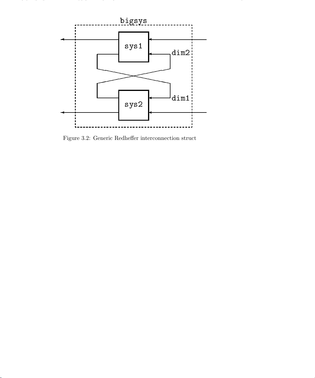
3.5. SYSTEM INTERCONNECTION 91

bigsys





`

`

`

sys1

`

sys2

`

`





`





`

dim2

`

dim1

Figure 3.2: Generic Redheffer interconnection structure

3.5 System Interconnection

Interconnections of systems are used extensively in the design, analysis and simulation
calculations. The most general form of interconnection, and the one used in forming
closed loop systems, is the Redheffer (or star) product. The Xµ function starp performs
this operation. This Redheffer product operation is illustrated in Figure 3.2. A MIMO
Dynamic System (or matrix) is created from two MIMO Dynamic Systems.

The syntax of the command to form this interconnection is,

bigsys = starp(sys1,sys2,dim1,dim2)

A more powerful, general, interconnection capability is given with the Xµ function
sysic. This can be used to interconnect subsystems (Dynamic Systems or constant
gain matrices) in an arbitrary manner. This is best illustrated by an example. Consider
the interconnection shown in Figure 3.3.

In each case it is assumed that the systems p, c,andwght, exist in the workspace prior
to calling sysic. The final four-input, three-output system is shown in Figure 3.4.

92 CHAPTER 3. FUNCTIONAL DESCRIPTION OF Xµ

act

6

7.5

6



t

c

1.6

6

tt



noise

noise

y



(1)

(2)

?

- -

l

+

-

?

wght

?

l

+

?

l

+

dist



p

Figure 3.3: Example interconnection of subsystems

act

err



y





clp









ref

dist

noise

noise

err

ref

l



+

,

6

(1)

(2)

Figure 3.4: Example interconnected system

3.5. SYSTEM INTERCONNECTION 93

Using sysic to form this interconnection can be considered as four distinct operations.

• Specify the individual subsystems.

• Name and dimension the input signals.

• Specify, algebraically in terms of subsystem outputs or input signals, the output of

the interconnected system.

• Specify, algebraically in terms of subsystem outputs or input signals, the input to

each of the subsystems.

• Name the closed loop system.

The Xµ script used to create the closed-loop system variable clp is shown below. A
single-input, two-output plant is considered. sysic is used to form the closed loop system
for a particular controller. Noise and disturbance signals, in addition to a command
reference, are considered as inputs. Tracking error and the control actuation are the
outputs of interest.

# form the subsystems

p1 = [1;1]*(1/makepoly([1,1,40],"s"));
p = daug(1,1/makepoly([1,1],"s"))*p1;
c = [50*makepoly([1,1],"s")/makepoly([1,10],"s"),-20];
wght = 0.01;

Name the subsystems - these must match with the workspace variables.

snames = ["p"; "c"; "wght"]

Name the final system inputs (names are arbitrary) Parenthesis are used to give a
dimension > 1.

inputs = ["ref"; "dist"; "noise(2)"]