National Instruments 370757C-01 User Manual

NI MATRIXx

XmathTM Robust Control Module

MATRIXx Xmath Robust Control Module

TM

April 2007
370757C-01

Support

Worldwide Technical Support and Product Information

ni.com

National Instruments Corporate Headquarters

11500 North Mopac Expressway Austin, Texas 78759-3504 USA Tel: [phone]

Worldwide Offices

Australia 1800 300 800, Austria 43 662 457990-0, Belgium 32 (0) 2 757 0020, Brazil 55 11 3262 3599,
Canada 800 433 3488, China 86 21 5050 9800, Czech Republic 420 224 235 774, Denmark 45 45 76 26 00,
Finland 385 (0) 9 725 72511, France 33 (0) 1 48 14 24 24, Germany 49 89 7413130, India 91 80 41190000,
Israel 972 3 6393737, Italy 39 02 413091, Japan 81 3 5472 2970, Korea 82 02 3451 3400,
Lebanon 961 (0) 1 33 28 28, Malaysia 1800 887710, Mexico 01 800 010 0793, Netherlands 31 (0) 348 433 466,
New Zealand 0800 553 322, Norway 47 (0) 66 90 76 60, Poland 48 22 3390150, Portugal 351 210 311 210,
Russia 7 495 783 6851, Singapore 1800 226 5886, Slovenia 386 3 425 42 00, South Africa 27 0 11 805 8197,
Spain 34 91 640 0085, Sweden 46 (0) 8 587 895 00, Switzerland 41 56 2005151, Taiwan 886 02 2377 2222,
Thailand 662 278 6777, Turkey 90 212 279 3031, United Kingdom 44 (0) 1635 523545

For further support information, refer to the Technical Support and Professional Services appendix. To comment
on National Instruments documentation, refer to the National Instruments Web site at ni.com/info and enter
the info code feedback.

© 2007 National Instruments Corporation. All rights reserved.

Important Information

Warranty

The media on which you receive National Instruments software are warranted not to fail to execute programming instructions, due to defects
in materials and workmanship, for a period of 90 days from date of shipment, as evidenced by receipts or other documentation. National
Instruments will, at its option, repair or replace software media that do not execute programming instructions if National Instruments receives
notice of such defects during the warranty period. National Instruments does not warrant that the operation of the software shall be
uninterrupted or error free.

A Return Material Authorization (RMA) number must be obtained from the factory and clearly marked on the outside of the package before any
equipment will be accepted for warranty work. National Instruments will pay the shipping costs of returning to the owner parts which are covered by
warranty.

National Instruments believes that the information in this document is accurate. The document has been carefully reviewed for technical accuracy. In
the event that technical or typographical errors exist, National Instruments reserves the right to make changes to subsequent editions of this document
without prior notice to holders of this edition. The reader should consult National Instruments if errors are suspected. In no event shall National
Instruments be liable for any damages arising out of or related to this document or the information contained in it.

XCEPT AS SPECIFIED HEREIN, NATIONAL INSTRUMENTS MAKES NO WARRANTIES, EXPRESS OR IMPLIED, AND SPECIFICALLY DISCLAIMS ANY WARRANTY OF

E

MERCHANTABILITY OR FITNESS FOR A PARTICULAR PURPOSE. C USTOMER’S RIGHT TO RECOVER DAMAGES CAUSED BY FAULT OR NEGLIGENCE ON THE PART OF NATIONAL

NSTRUMENTS SHALL BE LIMITED TO THE AMOUNT THERETOFORE PAID BY THE CUSTOMER. NATIONAL INSTRUMENTS WILL NOT BE LIABLE FOR DAMAGES RESULTING

I

FROM LOSS OF DATA, PROFITS, USE OF PRODUCTS, OR INCIDENTAL OR CONSEQUENTIAL DAMAGES, EVEN IF ADVISED OF THE POSSIBILITY THEREOF. This limitation of

the liability of National Instruments will apply regardless of the form of action, whether in contract or tort, including negligence. Any action against
National Instruments must be brought within one year after the cause of action accrues. National Instruments shall not be liable for any delay in
performance due to causes beyond its reasonable control. The warranty provided herein does not cover damages, defects, malfunctions, or service
failures caused by owner’s failure to follow the National Instruments installation, operation, or maintenance instructions; owner’s modification of the
product; owner’s abuse, misuse, or negligent acts; and power failure or surges, fire, flood, accident, actions of third parties, or other events outside
reasonable control.

Copyright

Under the copyright laws, this publication may not be reproduced or transmitted in any form, electronic or mechanical, including photocopying,
recording, storing in an information retrieval system, or translating, in whole or in part, without the prior written consent of National
Instruments Corporation.

National Instruments respects the intellectual property of others, and we ask our users to do the same. NI software is protected by copyright and other
intellectual property laws. Where NI software may be used to reproduce software or other materials belonging to others, you may use NI software only
to reproduce materials that you may reproduce in accordance with the terms of any applicable license or other legal restriction.

Trademarks

MATRIXx™, National Instruments™, NI™, ni.com™, and Xmath™ are trademarks of National Instruments Corporation. Refer to the Terms of
Use section on ni.com/legal for more information about National Instruments trademarks.

Other product and company names mentioned herein are trademarks or trade names of their respective companies.

Members of the National Instruments Alliance Partner Program are business entities independent from National Instruments and have no agency,
partnership, or joint-venture relationship with National Instruments.

Patents

For patents covering National Instruments products, refer to the appropriate location: Help»Patents in your software, the patents.txt file
on your CD, or

ni.com/patents.

WARNING REGARDING USE OF NATIONAL INSTRUMENTS PRODUCTS

(1) NATIONAL INSTRUMENTS PRODUCTS ARE NOT DESIGNED WITH COMPONENTS AND TESTING FOR A LEVEL OF
RELIABILITY SUITABLE FOR USE IN OR IN CONNECTION WITH SURGICAL IMPLANTS OR AS CRITICAL COMPONENTS IN
ANY LIFE SUPPORT SYSTEMS WHOSE FAILURE TO PERFORM CAN REASONABLY BE EXPECTED TO CAUSE SIGNIFICANT
INJURY TO A HUMAN.
(2) IN ANY APPLICATION, INCLUDING THE ABOVE, RELIABILITY OF OPERATION OF THE SOFTWARE PRODUCTS CAN BE
IMPAIRED BY ADVERSE FACTORS, INCLUDING BUT NOT LIMITED TO FLUCTUATIONS IN ELECTRICAL POWER SUPPLY,
COMPUTER HARDWARE MALFUNCTIONS, COMPUTER OPERATING SYSTEM SOFTWARE FITNESS, FITNESS OF COMPILERS
AND DEVELOPMENT SOFTWARE USED TO DEVELOP AN APPLICATION, INSTALLATION ERRORS, SOFTWARE AND HARDWARE
COMPATIBILITY PROBLEMS, MALFUNCTIONS OR FAILURES OF ELECTRONIC MONITORING OR CONTROL DEVICES,
TRANSIENT FAILURES OF ELECTRONIC SYSTEMS (HARDWARE AND/OR SOFTWARE), UNANTICIPATED USES OR MISUSES, OR
ERRORS ON THE PART OF THE USER OR APPLICATIONS DESIGNER (ADVERSE FACTORS SUCH AS THESE ARE HEREAFTER
COLLECTIVELY TERMED “SYSTEM FAILURES”). ANY APPLICATION WHERE A SYSTEM FAILURE WOULD CREATE A RISK OF
HARM TO PROPERTY OR PERSONS (INCLUDING THE RISK OF BODILY INJURY AND DEATH) SHOULD NOT BE RELIANT SOLELY
UPON ONE FORM OF ELECTRONIC SYSTEM DUE TO THE RISK OF SYSTEM FAILURE. TO AVOID DAMAGE, INJURY, OR DEATH,
THE USER OR APPLICATION DESIGNER MUST TAKE REASONABLY PRUDENT STEPS TO PROTECT AGAINST SYSTEM FAILURES,
INCLUDING BUT NOT LIMITED TO BACK-UP OR SHUT DOWN MECHANISMS. BECAUSE EACH END-USER SYSTEM IS
CUSTOMIZED AND DIFFERS FROM NATIONAL INSTRUMENTS' TESTING PLATFORMS AND BECAUSE A USER OR APPLICATION
DESIGNER MAY USE NATIONAL INSTRUMENTS PRODUCTS IN COMBINATION WITH OTHER PRODUCTS IN A MANNER NOT
EVALUATED OR CONTEMPLATED BY NATIONAL INSTRUMENTS, THE USER OR APPLICATION DESIGNER IS ULTIMATELY
RESPONSIBLE FOR VERIFYING AND VALIDATING THE SUITABILITY OF NATIONAL INSTRUMENTS PRODUCTS WHENEVER
NATIONAL INSTRUMENTS PRODUCTS ARE INCORPORATED IN A SYSTEM OR APPLICATION, INCLUDING, WITHOUT
LIMITATION, THE APPROPRIATE DESIGN, PROCESS AND SAFETY LEVEL OF SUCH SYSTEM OR APPLICATION.

Conventions

The following conventions are used in this manual:

[ ] Square brackets enclose optional items—for example, [

» The » symbol leads you through nested menu items and dialog box options

to a final action. The sequence File»Page Setup»Options directs you to
pull down the File menu, select the Page Setup item, and select Options
from the last dialog box.

This icon denotes a note, which alerts you to important information.

bold Bold text denotes items that you must select or click in the software, such

as menu items and dialog box options. Bold text also denotes parameter
names.

italic Italic text denotes variables, emphasis, a cross-reference, or an introduction

to a key concept. Italic text also denotes text that is a placeholder for a word
or value that you must supply.

monospace Text in this font denotes text or characters that you should enter from the

keyboard, sections of code, programming examples, and syntax examples.
This font is also used for the proper names of disk drives, paths, directories,
programs, subprograms, subroutines, device names, functions, operations,
variables, filenames, and extensions.

monospace bold Bold text in this font denotes the messages and responses that the computer

automatically prints to the screen. This font also emphasizes lines of code
that are different from the other examples.

response].

Contents

Chapter 1
Introduction

Using This Manual......................................................................................................... 1-1

Document Organization...................................................................................1-1

Bibliographic References ................................................................................1-2

Commonly-Used Nomenclature......................................................................1-2

Related Publications ........................................................................................ 1-2

MATRIXx Help...............................................................................................1-3

Overview........................................................................................................................1-3

Chapter 2
Robustness Analysis

Modeling Uncertain Systems.........................................................................................2-1

Stability Margin (smargin).............................................................................................2-3

smargin( ).........................................................................................................2-4

Worst-Case Performance Degradation (wcbode) ..........................................................2-8

wcbode( ).........................................................................................................2-9

Advanced Topics ...........................................................................................................2-10

Stability Margin...............................................................................................2-10

Stability Margin and Structured Singular

Stability Margin Bounds Using Singular Values..............................2-11

Approximation with Scaled Singular Values ....................................2-12

ssv( ) ................................................................................................................2-15

osscale( )..........................................................................................................2-16

pfscale( ) ..........................................................................................................2-16

optscale( ) ........................................................................................................2-17

Reducibility....................................................................................................................2-17

Worst-Case Performance Degradation (wcgain) ...........................................................2-18

Conversion to a Stability Margin Problem ...................................................... 2-18

wcgain( )..........................................................................................................2-19

Values (µ) .......................2-10

© National Instruments Corporation v MATRIXx Xmath Robust Control Module

Contents

Chapter 3
System Evaluation

Singular Value Bode Plots............................................................................................. 3-1

L Infinity Norm (linfnorm)............................................................................................ 3-3

linfnorm( ) ....................................................................................................... 3-4

Singular Value Bode Plots of Subsystems .................................................................... 3-7

perfplots( )....................................................................................................... 3-7

clsys( ) ............................................................................................................. 3-10

Chapter 4
Controller Synthesis

H-Infinity Control Synthesis ......................................................................................... 4-1

Problem Definition.......................................................................................... 4-1

Extended Transfer Matrix ............................................................................... 4-2

Building the Plant Model ................................................................................ 4-3

Weight Selection ............................................................................................. 4-5

Restrictions on the Extended Plant ................................................................. 4-7

hinfcontr( ) ...................................................................................................... 4-8

singriccati( ) .................................................................................................... 4-13

Linear-Quadratic-Gaussian Control Synthesis .............................................................. 4-14

LQG Frequency Shaping ................................................................................ 4-14

fsregu( ) ........................................................................................................... 4-14

fsesti( )............................................................................................................. 4-16

fslqgcomp( ) .................................................................................................... 4-17

Frequency-Shaped Control Design Commands.............................................. 4-17

Loop Transfer Recovery (lqgltr) ................................................................................... 4-22

lqgltr( ) ............................................................................................................ 4-23

Appendix A
Bibliography

Appendix B
Technical Support and Professional Services

Index

MATRIXx Xmath Robust Control Module vi ni.com

Introduction

The Xmath Robust Control Module (RCM) provides a collection of

analysis and synthesis tools that assist in the design of robust control

systems.

This chapter starts with an outline of the manual and some use notes. It

continues with an overview of the Xmath Robust Control Module (RCM)

functions.

Using This Manual

This manual provides complete documentation for all the RCM functions

along with their associated theoretical background, references, and

examples.

Document Organization

This manual includes the following chapters:

• Chapter 1, Introduction, describes the Robust Control Module (RCM)
and shows the RCM function structure.

• Chapter 2, Robustness Analysis, covers the robustness analysis
tools and introduces the concepts of uncertainty, robustness, and
performance degradation in the framework of closed-loop systems.
The Modeling Uncertain Systems section should be read by all those
interested in robustness analysis or performance degradation, which
are explained in the Stability Margin (smargin) section and the

Worst-Case Performance Degradation (wcbode) section. The
Advanced Topics section provides additional information but this

material is not prerequisite to the use of RCM functions.

• Chapter 3, System Evaluation, describes system analysis functions that
create singular value Bode plots, performance plots, and calculate the

L

users.

• Chapter 4, Controller Synthesis, discusses synthesis tools in two
categories, H
of the theory of H

1

norm of a linear system. This chapter should be of interest to all

∞

and H2. This manual does not attempt to explain all

∞

, LQG/LTR, and frequency shaped LQG design

∞

© National Instruments Corporation 1-1 MATRIXx Xmath Robust Control Module

Chapter 1 Introduction

techniques. The general problem setup is explained together with
known limitations; the rest is left to the references.

Bibliographic References

Throughout this document, bibliographic references are cited with
bracketed entries. For example, a reference to [DoS81] corresponds
to a document published by Doyle and Stein in 1981. For a table of
bibliographic references, refer to Appendix A, Bibliography.

Commonly-Used Nomenclature

This manual uses the following general nomenclature:

• Matrix variables are generally denoted with capital letters; vectors are
represented in lowercase.

• G(s) is used to denote a transfer function of a system where s is the
Laplace variable. G(q) is used when both continuous and discrete
systems are allowed.

• H(s) is used to denote the frequency response, over some range of
frequencies of a system where s is the Laplace variable. H(q) is used to
indicate that the system can be continuous or discrete.

• A single apostrophe following a matrix variable, for example, x
denotes the transpose of that variable. An asterisk following a matrix
variable (for example, A*) indicates the complex conjugate, or
Hermitian, transpose of that variable.

'

,

Related Publications

For a complete list of MATRIXx publications, refer to Chapter 2,

MATRIXx Publications, Help, and Online Support, of the MATRIXx
Getting Started Guide. The following documents are particularly useful

for topics covered in this manual:

• MATRIXx Getting Started Guide

• Xmath User Guide

• Xmath Control Design Module

• Xmath Interactive Control Design Module

• Xmath Interactive System Identification Module, Part 1

• Xmath Interactive System Identification Module, Part 2

• Xmath Model Reduction Module

MATRIXx Xmath Robust Control Module 1-2 ni.com

MATRIXx Help

Overview

Chapter 1 Introduction

• Xmath Optimization Module

• Xmath Robust Control Module

• Xmath X

Robust Control Module function reference information is available in the
MATRIXx Help. The MATRIXx Help includes all Robust Control functions.
Each topic explains a function’s inputs, outputs, and keywords in detail.
Refer to Chapter 2, MATRIXx Publications, Help, and Online Support, of
the MATRIXx Getting Started Guide for complete instructions on using the
Help feature.

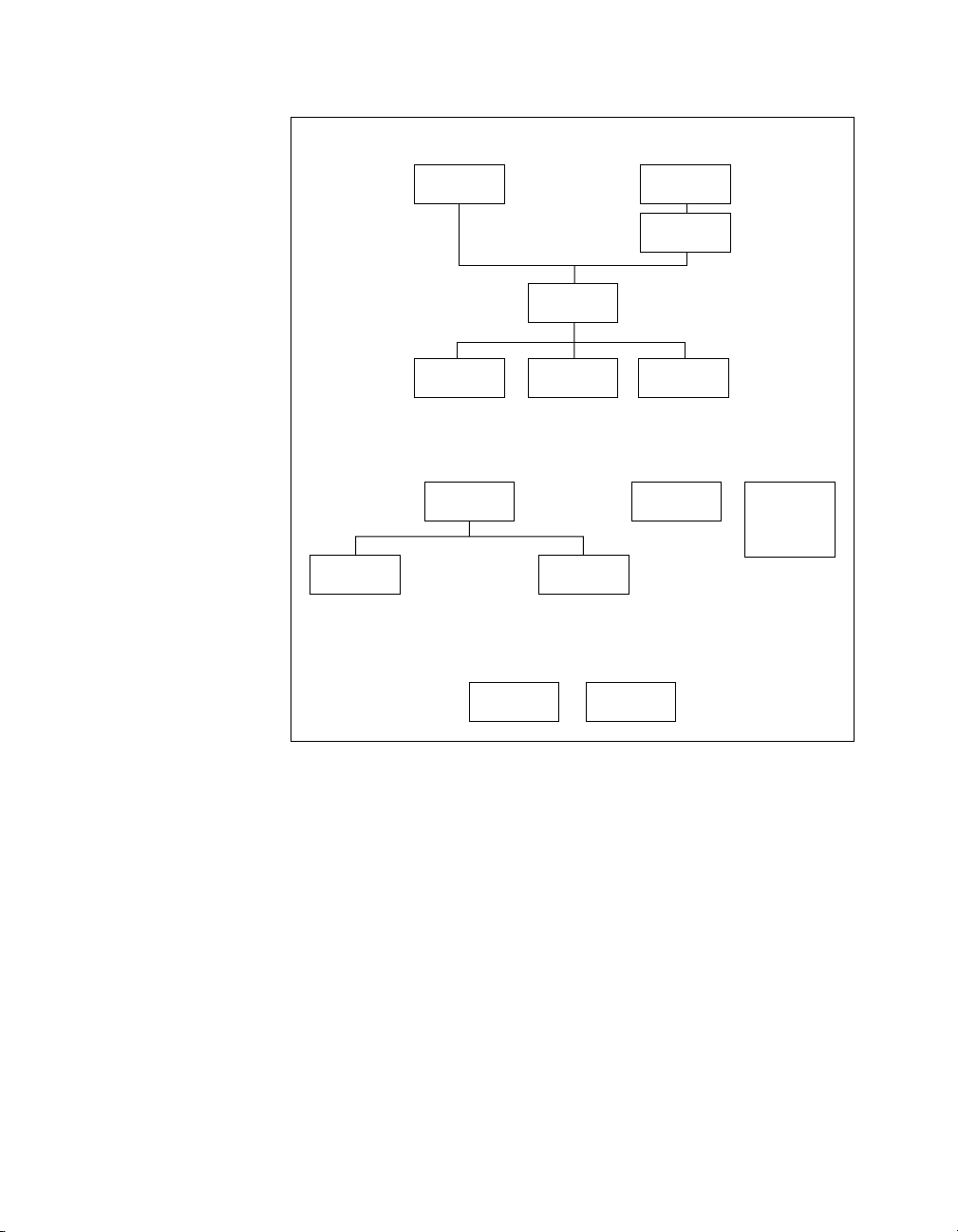
RCM functionality is structured as shown in Figure 1-1.

μ

Module

© National Instruments Corporation 1-3 MATRIXx Xmath Robust Control Module

Chapter 1 Introduction

Analysis Functions

smargin

ssv

pfscale optscale osscale

Synthesis Functions

hinfcontr

singriccati clsys

Utility Functions

wcbode

wcgain

lqgltr

perfplotslinfnorm

fslqgcomp

fsesti

fsregu

Figure 1-1. RCM Function Structure

Many RCM functions are based on state-of-the-art algorithms implemented
in cooperation with researchers at Stanford University. The robustness
analysis functions are based on structured singular value calculations.
The synthesis tools expand on existing LQG (H
and frequency shaping) while adding new H

MATRIXx Xmath Robust Control Module 1-4 ni.com

) techniques (LQG/LTR

2

design functions.

∞

Robustness Analysis

z

This chapter describes RCM tools used for analyzing the robustness
of a closed-loop system. The chapter assumes that a controller has been
designed for a nominal plant and that the closed-loop performance of
this nominal system is acceptable. The goal of robustness analysis is to
determine whether the performance will remain acceptable if the plant
differs from the nominal plant.

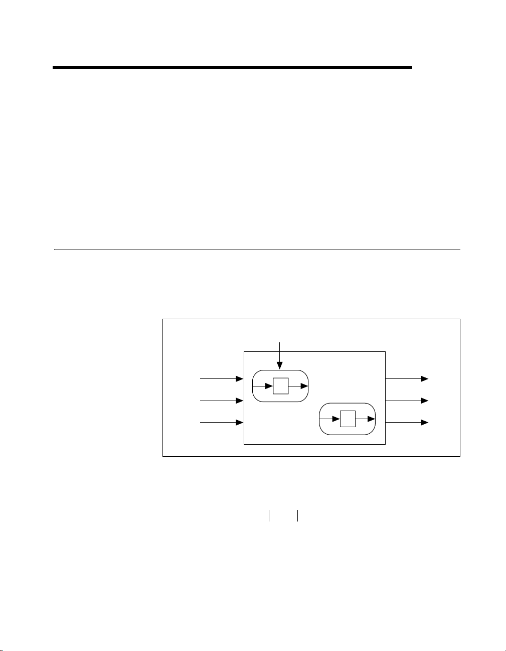
Modeling Uncertain Systems

This section describes the method RCM uses to model an uncertain system.
The closed-loop system is modeled as a known or nominal closed-loop
system with input w and output z, together with k unknown or uncertain
transfer functions δ

w

(jω), …, δk(jω), as shown in Figure 2-1.

1

Uncertain Transfer Function

2

Known Nominal

q

r

1

1

δ

1

System

q

r

2

2

δ

2

Figure 2-1. Model of an Uncertain System

The following transfer functions are assumed to be stable:

δijω()lijω()≤

where the l
uncertainty model is known as structured nonparametric uncertainties.
To describe this model, you also must describe the nominal closed-loop

© National Instruments Corporation 2-1 MATRIXx Xmath Robust Control Module

are given non-negative functions of frequency. This type of

i

(2-1)

Chapter 2 Robustness Analysis

system, including how the uncertain transfer functions are connected to the
system and the magnitude bound functions l

(w).

i

To do this, extract the uncertain transfer functions and collect them into a

k-input, k-output transfer matrix Δ, where:

Δ jω() diagonal δ

jω(),...,δkjω()()=

1

(2-2)

The resulting closed-loop system can be viewed as a feedback connection
of the nominal closed-loop system with transfer matrix H(jω) and the
uncertain transfer matrix Δ( jω). You describe your nominal closed-loop
system as a linear system with

w

input and output .

r

Note The signals r and q are not really inputs and outputs of the nominal system; r and q

z

q

show how the uncertain transfer functions connect to your nominal system. The signals r
and q each have k components.

You will partition H into the four submatrices,

H

H

so that H
transfer matrix from r to z, H
and H

is the nominal transfer matrix from w to z, Hzr is the nominal

zw

qw

is the nominal transfer matrix from r to q.

qr

The magnitude bound functions l
with the PDM

delb:

zwHzr

=

HqwH

qr

is the nominal transfer matrix from w to q,

(jω) from Equation 2-1 are described

i

ω

l1ω1()…lkω1()

1

DELB

Thus, a complete description of your system requires the system
to represent H

MATRIXx Xmath Robust Control Module 2-2 ni.com

and the response delb to represent the bounds.

jw

=

,

:

ω

m

::

()…lkωm()

l

1ωm

SysH

Stability Margin (smargin)

Assume that the nominal closed-loop system is stable. That belief raises a
question: Does the system remain stable for all possible uncertain transfer
functions that satisfy the magnitude bounds (Equation 2-1)? If so, the
system is said to be robustly stable. If the magnitude bounds are small
enough, the uncertainties will not destabilize the system; your system will
be robustly stable.

Roughly speaking, the stability margin of your system is defined as the
factor by which you can increase all the magnitude bounds l
maintain stability for all possible uncertain transfer functions δ
number is larger than one (0 dB), then you know that there are no uncertain
transfer functions that satisfy the magnitude bound and destabilize your
system. Moreover, the number tells you how much more uncertainty your
system could tolerate than the given bounds l
one, then there are uncertain transfer functions that satisfy the magnitude
bound (Equation 2-1) and result in an unstable system. In this case, the
margin tells you how much you must reduce the magnitude bounds before
you have robust stability.

More precisely, the stability margin at frequency ω is defined as the
smallest α such that the system can have a pole at jω, with the uncertain
transfer functions satisfying |δ

(jω)| ≤ αli(ω):

i

Chapter 2 Robustness Analysis

and still

i

. If this

i

(ω). If the margin is less than

i

margin(w) = min{ α| systems can have a pole at jω with magnitude bounds αl

(jω)}

i

The stability margin also can be expressed as:

margin(w) = min{ α| det I – H

Note The stability margin only depends on H

jωΔ ≠ 0 such that |Δii|≤αli(α)}

qr

.

qr

The margin often is expressed in dB. If the margin is greater than zero for
all frequencies, then your system is robustly stable. If the margin is less
than zero for some frequencies, then your system is not robustly stable.
In particular, there are uncertain transfer functions that satisfy the
magnitude bound (Equation 2-1) and cause the system to have a pole at
those frequencies where the margin is negative. This does not mean that any

values that satisfy the magnitude bound will destabilize the system: it

δ

i

means that there are some bad δ

values that satisfy the magnitude bounds

i

and destabilize the system.

© National Instruments Corporation 2-3 MATRIXx Xmath Robust Control Module

Chapter 2 Robustness Analysis

z

q

smargin( )

marg = smargin(SysH, delb {scaling, graph})

The smargin( ) function plots an approximation to the stability margin
of the system as a function of frequency. For a full discussion of

smargin( ) syntax, refer to the MATRIXx Help. The approximation is

exact if the number of uncertain transfer functions is less than four and

scaling="OPT" (optimum scaling).

In other cases, the approximation is generally considered to be extremely
good. Refer to the Approximation with Scaled Singular Values section. The
approximation is always conservative.

smargin( ) always will report a

margin that is less than or equal to the actual margin.

smargin( ) function counts the columns in delb to calculate the

The
number of uncertainties k. It then assumes that the last k inputs of

SysH are

signal r in Figure 2-2, and the last k outputs are signal q. To create a Nominal
System, refer to the Creating a Nominal System section.

w

Known Closed-Loop System

r

size

k

Figure 2-2. Nominal Closed-Loop System

H(s)

size

k

Creating a Nominal System

To better understand how to create H(s) in Figure 2-3, you will examine
a SISO tracking system with three uncertainties. δ
actuator uncertainty, while δ

and δ3 are multiplicative sensor uncertainties.

2

is a multiplicative

1

MATRIXx Xmath Robust Control Module 2-4 ni.com

Chapter 2 Robustness Analysis

reference

8

––

reference

+

1

+

1
s

+

= 4

K

1

x

1

1

+

+

K2 = 8

+

–

error

x

2

1
s

2

+

+

Figure 2-3. SISO Tracking System with Three Uncertainties

The H system will have the reference input as input1 and the error output
as output1 (w and z, respectively, in Figure 2-2). Removing the δ values will
create inputs 2 through 4 and outputs 2 through 4 (r and q, respectively, in
Figure 2-2).

1. The A, B, C, D matrices of the state-space system representing H are
as follows:

A=[-4,-8;1,0];

B=[8,1,-4,-8;zeros(1,4)];

C=[0,-1;-4,-8;1,0;0,1];

D=[1,0,0,0;8,0,-4,-8;zeros(2,4)];

H = system(A,B,C,D,{inputNames=["reference",

"r1","r2","r3"],outputNames=["error",

"q1","q2","q3"],stateNames=["x1","x2"]});

2. Specify the uncertainty bounds.

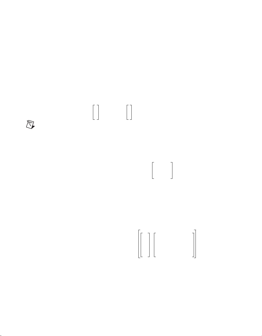
The sensor uncertainty δ
to Equation 2-1. Because the position x

is known to be bounded by l3(w), according

3

sensor model is known to be

2

accurate to 10% up to one radian per second, and very inaccurate at
high frequencies, the l

shown in Figure 2-4 is selected.

3

© National Instruments Corporation 2-5 MATRIXx Xmath Robust Control Module

Chapter 2 Robustness Analysis

dB

10

0

–20

0.1

1

Frequency, Radian/Second

30 100

Figure 2-4. Bound for Sensor Uncertainty

Note

A value of l3 at one radian per second of –20 dB indicates that modeling

uncertainties of up to 10% (–20 dB = 0.1) are allowed.

The actuator and sensor uncertainties δ

and δ2 are bounded by –20 dB

1

at all frequencies. You will use these values to interpolate to obtain l
First, create the bound for δ

L3 = pdm([-20,-20,10,10],[0.1,1,30,100]/2/pi);

in Hz.

3

3. Now interpolate to obtain 30 points:

L3 = interpolate(L3,logspace(0.01,10,30),{xlog});

4. Create L1 and L2 (bounds for and ):

δ

δ

1

2

L1=-20*ones(L3); L2 = L1;

delb = [L1,L2,L3];

5. Calculate the stability margin:

marg=smargin(H,delb);

smargin --> Scaling algorithm is type: PF

smargin --> Margin computation 10% complete

smargin --> Margin computation 50% complete

smargin --> Margin computation 90% complete

The output indicates that Perron-Frobenius scaling (the default) is
used. Refer to the Approximation with Scaled Singular Values section.

The stability margin plot is shown in Figure 2-5. The minimum margin
is about 8 dB at about 1/2 Hz. This implies that all three l
(uncertainty bounds) could be increased (relaxed) simultaneously
by 8 dB, and the system would still remain robustly stable.

values

1

.

3

MATRIXx Xmath Robust Control Module 2-6 ni.com

Chapter 2 Robustness Analysis

Figure 2-5. Stability Margin

Now examine the effect on the stability margin of discretizing H(s) at
100 Hz.

dt = 0.01;

Hd = discretize(H,dt);

margD = smargin(Hd,delb);

smargin --> Scaling algorithm is type: PF

smargin --> Margin computation 10% complete

smargin --> Margin computation 50% complete

smargin --> Margin computation 90% complete

100 Hz is a high discretization frequency for H, so the stability margin
is unchanged in the discrete-time case. The new plot is not much
different from Figure 2-6. Again, minimum margin is about 8 dB
at about 1/2 Hz.

© National Instruments Corporation 2-7 MATRIXx Xmath Robust Control Module

Chapter 2 Robustness Analysis

Worst-Case Performance Degradation (wcbode)

Even if a system is robustly stable, the uncertain transfer functions still can
have a great effect on performance. Consider the transfer function from the
qth input, w
nominal system, and this transfer function is the p,q entry of H
called the nominal transfer function.

, to the pth output, zp. With δ1 = ... = ...δk = 0, you have the

q

. This is

zw

When the δ values are not zero, the transfer function from w
entry of H

given by the formula:

pert

H

HzwHzrΔ IHqrΔ–()

pert

1–

+=

H

to zp is the p,q

q

qw

This is referred to as the perturbed transfer function. The perturbed transfer
function depends on the particular δ

, …, δk.

1

If the magnitude bounds are small enough, then you expect the perturbed
transfer function H

to be close to the nominal transfer function. Roughly

pert

speaking, small perturbations should not significantly alter the closed-loop
transfer function from w

to zp.

q

The worst-case gain is defined as the largest magnitude of the perturbed
transfer function, considering all δ values that satisfy the magnitude bound.
More precisely:

wcgain ω() max H

pert,pq

wcgain(ω) is always larger than the nominal gain, |H

Δ = diagonal δ1,...,δ

()δiliω()≤,{}=

k

(jω)|. This is not

zw,pq

because the uncertain transfer functions only can increase the magnitude of
the transfer function from w

to zq. In fact, it is possible that for a lucky

q

choice of the δ values, the perturbed transfer function actually can be
smaller than the nominal transfer function over all frequencies. But in the
worst-case gain, you consider only the worst possible δ values, and these
always increase the perturbed gain over the nominal gain.

(2-3)

Intuitively, if the stability margin is large, then the uncertain transfer
functions should not greatly effect the gain from w
should be not much larger than the nominal gain |H

to zp, so that wcgain(ω)

q

(jω)|. If the stability

zw,pq

margin is small, however, wcgain(ω) could be much larger than the nominal
gain. An extreme case occurs if the stability margin is negative (in dB) at
the frequency δ. Then you have wcgain(ω) = ∞, although

wcbode( ) clips

the worst-case gain curve so that it never exceeds (the maximum nominal
gain) * 100, or +20 dB. Of course, instability is an extreme form of
performance degradation.

MATRIXx Xmath Robust Control Module 2-8 ni.com

wcbode( )

Chapter 2 Robustness Analysis

[WCMAG, NOMMAG] = wcbode (SysH, delb, {input, output,

graph})

The wcbode( ) function computes and plots the worst-case gain of a
closed-loop transfer function.

This function is useful for checking a system that already has been verified
to be robustly stable using

smargin( ). For example, a system can have a

minimum stability margin of 4 dB, so it is robustly stable. If the worst-case
gain from a function input to the output it commands has a 20 dB peak, then
even though the system is robustly stable, the design is unacceptable. On
the other hand, if you verify that the perturbed closed-loop transfer function
increases only 2 dB over the nominal, then the design is probably
acceptable.

wcbode( ) function computes and plots an approximation to

The
wcgain(ω), the largest possible magnitude of a perturbed closed-loop
transfer function that can be caused by uncertain transfer functions that
satisfy the magnitude bound. The

wcbode( ) function is conservative:

it does not under-report the maximum of the perturbed transfer function.

A large value of

wcbode( ) returns a maximum value of ten times the maximum of

case,

wcbode( ) indicates instability: wcgain(ω) = ∞. In this

the nominal transfer function over all frequencies. Consequently, the
window is clipped at 20 dB above the maximum of the nominal transfer
function over all frequencies.

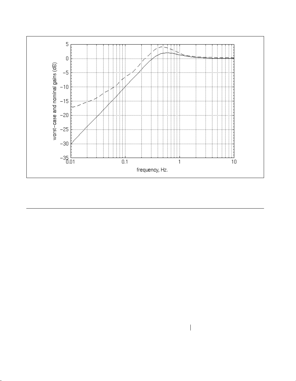
The wcbode( ) function also plots the

nominal transfer function for reference.

Using wcbode( ) to Analyze Performance Degradation

The wcbode( ) function can be used to analyze performance degradation
for the system you have been using (Figure 2-3). The transfer function,
which should be small, is from reference to error (input 1 to output 1).
Figure 2-6 shows the results of the following function call:

[NOMMAG,WCMAG]=wcbode(H,delb,{input=1,output=1});

The performance degradation due to the uncertainties is small but not
negligible.

© National Instruments Corporation 2-9 MATRIXx Xmath Robust Control Module

Chapter 2 Robustness Analysis

Figure 2-6. Performance Degradation of the SISO Tracking System

Advanced Topics

This section describes the theoretical background on robustness analysis
and performance degradation.

Stability Margin

This section discusses advanced aspects of computing the stability margin
and the related scaling algorithms.

Stability Margin and Structured Singular Values (μ)

The stability margin was first defined by Safonov in [Saf82]. If you let

MHqrdiagonal l1w()...,lkw(),()=

then you can express the margin at frequency d as

margin ω() max= α det I MΔ–()0≠{

MATRIXx Xmath Robust Control Module 2-10 ni.com

for all diagonal Δ such that

Chapter 2 Robustness Analysis

1

-------------=

μ M()

where μ(

Δiiα≤()}

.

) is the structured singular value, introduced by Doyle in

[Doy82]. Thus, the margin is the inverse of the structured singular value of

diagonally scaled by the magnitude bounds.

H

qr

There is no numerically efficient algorithm that is guaranteed to compute
μ(M), and hence the stability margin. However, it is possible to compute
various good approximations to μ(M). One of these approximations is often
exact.

Stability Margin Bounds Using Singular Values

A popular but conservative method uses singular values:

1

----------------------

margin ω()

Plotting the right side of Equation 2-4 gives a lower bound on the
actual stability margin. To get this plot, specify

scaling="SVD". This approximation can be very conservative, meaning

that the left side can be much larger than the right side. This fact spurred
the study of structured singular values and the other approximations
discussed in the following sections.

≥

σ

max

M()

smargin( ) with

(2-4)

Use of Scaling Example

For this example, you will use the system in Figure 2-3. This time

smargin( ) will be invoked with scaling="SVD", so smargin( )

will calculate Equation 2-4.

margSVD = smargin(H,delb,{scaling="SVD"});

smargin --> Scaling algorithm is type: SVD

smargin --> Margin computation 10% complete

smargin --> Margin computation 50% complete

smargin --> Margin computation 90% complete

© National Instruments Corporation 2-11 MATRIXx Xmath Robust Control Module

Chapter 2 Robustness Analysis

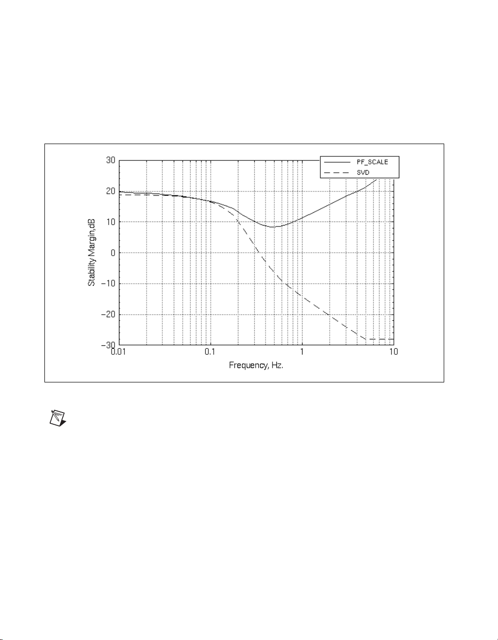
You can compare this margin to that of the example in the Creating a

Nominal System section; the following inputs produce Figure 2-7.

plot ([marg,margSVD],{xlog}

legend=["PF_SCALE","SVD"],

ylab="Stability Margin,dB",

xlab="Frequency, Hz."})

Figure 2-7. pfscale( ) versus svd Stability Margins

Note

The singular value approach gives results that are too conservative, suggesting that
the uncertainties can destabilize the system. Conversely, you know from the scaled singular
value calculations that the system is robustly stable.

Approximation with Scaled Singular Values

In [Saf82] and [Doy82], the inequality

min σ

D diagonal

()μM()≥

max

is noted. This optimization problem can be shown to be
unimodal—for D>0, an assumption that can be made without loss

MATRIXx Xmath Robust Control Module 2-12 ni.com

DMD

1–

(2-5)