

Page 1

TM
MATRIXx
XmathTM Model Reduction Module
Xmath Model Reduction Module
April 2004 Edition
Part Number 370755B-01
Page 2

Support
Worldwide Technical Support and Product Information
ni.com
National Instruments Corporate Headquarters
11500 North Mopac Expressway Austin, Texas 78759-3504 USA Tel: 512 683 0100
Worldwide Offices
Australia1800300800, Austria4306624579900, Belgium32027570020, Brazil551132623599,
Canada (Calgary) 403 274 9391, Canada (Ottawa) 613 233 5949, Canada (Québec) 450 510 3055,
Canada (Toronto) 905 785 0085, Canada (Vancouver) 514 685 7530, China 86 21 6555 7838,
Czech Republic 420 224 235 774, Denmark 45 45 76 26 00, Finland 3850972572511,
France330148142424, Germany490897413130, Greece302104296427, India918051190000,
Israel972036393737, Italy3902413091, Japan81354722970, Korea820234513400,
Malaysia 603 9131 0918, Mexico 001 800 010 0793, Netherlands 31 0 348 433 466,
New Zealand 0800 553 322, Norway 47 0 66 90 76 60, Poland 48 22 3390150, Portugal 351 210 311 210,
Russia 7 095 783 68 51, Singapore 65 6226 5886, Slovenia 386 3 425 4200, South Africa 27 0 11 805 8197,
Spain34916400085, Sweden460858789500, Switzerland41562005151, Taiwan886225287227,
Thailand 662 992 7519, United Kingdom 44 0 1635 523545
For further support information, refer to the Technical Support and Professional Services appendix. To comment
on the documentation, send email to techpubs@ni.com.
© 2000–2004 National Instruments Corporation. All rights reserved.
Page 3

Important Information
Warranty
The media on which you receive National Instruments software are warranted not to fail to execute programming instructions, due to defects
in materials and workmanship, for a period of 90 days from date of shipment, as evidenced by receipts or other documentation. National
Instruments will, at its option, repair or replace software media that do not execute programming instructions if National Instruments receives
notice of such defects during the warranty period. National Instruments does not warrant that the operation of the software shall be
uninterrupted or error free.
A Return Material Authorization (RMA) number must be obtained from the factory and clearly marked on the outside of the package before
any equipment will be accepted for warranty work. National Instruments will pay the shipping costs of returning to the owner parts which are
covered by warranty.
National Instruments believes that the information in this document is accurate. The document has been carefully reviewed for technical
accuracy. In the event that technical or typographical errors exist, National Instruments reserves the right to make changes to subsequent
editions of this document without prior notice to holders of this edition. The reader should consult National Instruments if errors are suspected.
In no event shall National Instruments be liable for any damages arising out of or related to this document or the information contained in it.
E
XCEPT AS SPECIFIED HEREIN, NATIONAL INSTRUMENTS MAKES NO WARRANTIES, EXPRESS OR IMPLIED, AND SPECIFICALLY DISCLAIMS ANY WARRANTY OF
MERCHANTABILITY OR FITNESS FOR A PARTICULAR PURPOSE. CUSTOMER’S RIGHT TO RECOVER DAMAGES CAUSED BY FAULT OR NEGLIGENCE ON THE PART OF
N
ATIONAL INSTRUMENTS SHALL BE LIMITED TO THE AMOUNT THERETOFORE PAID BY THE CUSTO MER. NATIONAL INSTRUMENTS WILL NOT BE LIA BLE FOR
DAMAGES RESULTIN G FROM LOSS OF DATA, PROFITS, USE OF PRODUCTS, OR INCIDENTAL OR CONSEQUENTIAL DAMAGES, EVEN IF ADVI SED OF THE POSSIB ILITY
THEREOF. This limitation of the liability of National Instruments will apply regardless of the form of action, whether in contract or tort, including
negligence. Any action against National Instruments must be brought within one year after the cause of action accrues. National Instruments
shall not be liable for any delay in performance due to causes beyond its reasonable control. The warranty provided herein does not cover
damages, defects, malfunctions, or service failures caused by owner’s failure to follow the National Instruments installation, operation, or
maintenance instructions; owner’s modification of the product; owner’s abuse, misuse, or negligent acts; and power failure or surges, fire,
flood, accident, actions of third parties, or other events outside reasonable control.
Copyright
Under the copyright laws, this publication may not be reproduced or transmitted in any form, electronic or mechanical, including photocopying,
recording, storing in an information retrieval system, or translating, in whole or in part, without the prior written consent of National
Instruments Corporation.
Trademarks
MATRIXx™, National Instruments™, NI™, ni.com™, and Xmath™ are trademarks of National Instruments Corporation.
Product and company names mentioned herein are trademarks or trade names of their respective companies.
Patents
For patents covering National Instruments products, refer to the appropriate location: Help»Patents in your software, the patents.txt file
on your CD, or ni.com/patents.
WARNING REGARDING USE OF NATIONAL INSTRUMENTS PRODUCTS
(1) NATIONAL INSTRUMENTS PRODUCTS ARE NOT DESIGNED WITH COMPONENTS AND TESTING FOR A LEVEL OF
RELIABILITY SUITABLE FOR USE IN OR IN CONNECTION WITH SURGICAL IMPLANTS OR AS CRITICAL COMPONENTS IN
ANY LIFE SUPPORT SYSTEMS WHOSE FAILURE TO PERFORM CAN REASONABLY BE EXPECTED TO CAUSE SIGNIFICANT
INJURY TO A HUMAN.
(2) IN ANY APPLICATION, INCLUDING THE ABOVE, RELIABILITY OF OPERATION OF THE SOFTWARE PRODUCTS CAN BE
IMPAIRED BY ADVERSE FACTORS, INCLUDING BUT NOT LIMITED TO FLUCTUATIONS IN ELECTRICAL POWER SUPPLY,
COMPUTER HARDWARE MALFUNCTIONS, COMPUTER OPERATING SYSTEM SOFTWARE FITNESS, FITNESS OF COMPILERS
AND DEVELOPMENT SOFTWARE USED TO DEVELOP AN APPLICATION, INSTALLATION ERRORS, SOFTWARE AND
HARDWARE COMPATIBILITY PROBLEMS, MALFUNCTIONS OR FAILURES OF ELECTRONIC MONITORING OR CONTROL
DEVICES, TRANSIENT FAILURES OF ELECTRONIC SYSTEMS (HARDWARE AND/OR SOFTWARE), UNANTICIPATED USES OR
MISUSES, OR ERRORS ON THE PART OF THE USER OR APPLICATIONS DESIGNER (ADVERSE FACTORS SUCH AS THESE ARE
HEREAFTER COLLECTIVELY TERMED “SYSTEM FAILURES”). ANY APPLICATION WHERE A SYSTEM FAILURE WOULD
CREATE A RISK OF HARM TO PROPERTY OR PERSONS (INCLUDING THE RISK OF BODILY INJURY AND DEATH) SHOULD
NOT BE RELIANT SOLELY UPON ONE FORM OF ELECTRONIC SYSTEM DUE TO THE RISK OF SYSTEM FAILURE. TO AVOID
DAMAGE, INJURY, OR DEATH, THE USER OR APPLICATION DESIGNER MUST TAKE REASONABLY PRUDENT STEPS TO
PROTECT AGAINST SYSTEM FAILURES, INCLUDING BUT NOT LIMITED TO BACK-UP OR SHUT DOWN MECHANISMS.
BECAUSE EACH END-USER SYSTEM IS CUSTOMIZED AND DIFFERS FROM NATIONAL INSTRUMENTS' TESTING
PLATFORMS AND BECAUSE A USER OR APPLICATION DESIGNER MAY USE NATIONAL INSTRUMENTS PRODUCTS IN
COMBINATION WITH OTHER PRODUCTS IN A MANNER NOT EVALUATED OR CONTEMPLATED BY NATIONAL
INSTRUMENTS, THE USER OR APPLICATION DESIGNER IS ULTIMATELY RESPONSIBLE FOR VERIFYING AND VALIDATING
THE SUITABILITY OF NATIONAL INSTRUMENTS PRODUCTS WHENEVER NATIONAL INSTRUMENTS PRODUCTS ARE
INCORPORATED IN A SYSTEM OR APPLICATION, INCLUDING, WITHOUT LIMITATION, THE APPROPRIATE DESIGN,
PROCESS AND SAFETY LEVEL OF SUCH SYSTEM OR APPLICATION.
Page 4

Conventions
The following conventions are used in this manual:
[ ] Square brackets enclose optional items—for example, [
brackets also cite bibliographic references.
» The » symbol leads you through nested menu items and dialog box options
to a final action. The sequence File»Page Setup»Options directs you to
pull down the File menu, select the Page Setup item, and select Options
from the last dialog box.
This icon denotes a note, which alerts you to important information.
bold Bold text denotes items that you must select or click in the software, such
as menu items and dialog box options. Bold text also denotes parameter
names.
italic Italic text denotes variables, emphasis, a cross reference, or an introduction
to a key concept. This font also denotes text that is a placeholder for a word
or value that you must supply.
monospace Text in this font denotes text or characters that you should enter from the
keyboard, sections of code, programming examples, and syntax examples.
This font is also used for the proper names of disk drives, paths, directories,
programs, subprograms, subroutines, device names, functions, operations,
variables, filenames, and extensions.
monospace bold Bold text in this font denotes the messages and responses that the computer
automatically prints to the screen. This font also emphasizes lines of code
that are different from the other examples.
response]. Square
monospace italic Italic text in this font denotes text that is a placeholder for a word or value
that you must supply.
Page 5

Contents
Chapter 1
Introduction
Using This Manual.........................................................................................................1-1
Document Organization...................................................................................1-1
Bibliographic References ................................................................................1-2
Commonly Used Nomenclature ......................................................................1-2
Conventions.....................................................................................................1-2
Related Publications ........................................................................................1-3
MATRIXx Help...............................................................................................1-3
Overview........................................................................................................................1-3
Functions .........................................................................................................1-4
Nomenclature .................................................................................................1-6
Commonly Used Concepts ............................................................................................1-7
Controllability and Observability Grammians ................................................1-7
Hankel Singular Values...................................................................................1-8
Internally Balanced Realizations.....................................................................1-10
Singular Perturbation.......................................................................................1-11
Spectral Factorization......................................................................................1-13
Low Order Controller Design Through Order Reduction .............................................1-15
Chapter 2
Additive Error Reduction
Introduction....................................................................................................................2-1
Truncation of Balanced Realizations.............................................................................2-2
Reduction Through Balanced Realization Truncation...................................................2-4
Singular Perturbation of Balanced Realization..............................................................2-5
Hankel Norm Approximation ........................................................................................2-6
balmoore( ).....................................................................................................................2-8
Related Functions ............................................................................................2-11
truncate( ).......................................................................................................................2-11
Related Functions ............................................................................................2-11
redschur( )......................................................................................................................2-12
Algorithm ........................................................................................................2-12
Related Functions ............................................................................................2-14
ophank( ) ........................................................................................................................2-14
Restriction........................................................................................................2-14
Algorithm ........................................................................................................2-15
Behaviors.........................................................................................................2-15
© National Instruments Corporation v Xmath Model Reduction Module
Page 6

Contents
Onepass Algorithm ......................................................................................... 2-18
Multipass Algorithm ...................................................................................... 2-20
Discrete-Time Systems ................................................................................... 2-21
Impulse Response Error.................................................................................. 2-22
Unstable System Approximation .................................................................... 2-23
Related Functions............................................................................................ 2-23
Chapter 3
Multiplicative Error Reduction
Selecting Multiplicative Error Reduction......................................................................3-1
Multiplicative Robustness Result.................................................................... 3-2
bst( )............................................................................................................................... 3-3
Restrictions...................................................................................................... 3-4
Algorithm ........................................................................................................ 3-4
Algorithm with the Keywords right and left................................................... 3-5
Securing Zero Error at DC.............................................................................. 3-8
Hankel Singular Values of Phase Matrix of G
Further Error Bounds ...................................................................................... 3-9
Reduction of Minimum Phase, Unstable G .................................................... 3-9
Imaginary Axis Zeros (Including Zeros at ∞)................................................. 3-10
Related Functions............................................................................................ 3-14
mulhank( ) ..................................................................................................................... 3-14
Restrictions...................................................................................................... 3-14
Algorithm ........................................................................................................ 3-14
right and left .................................................................................................... 3-15
Consequences of Step 5 and Justification of Step 6........................................ 3-18
Error Bounds................................................................................................... 3-20
Imaginary Axis Zeros (Including Zeros at ∞)................................................. 3-21
Related Functions............................................................................................ 3-24
............................................... 3-9
r
Chapter 4
Frequency-Weighted Error Reduction
Introduction ................................................................................................................... 4-1
Controller Reduction....................................................................................... 4-2
Controller Robustness Result.......................................................................... 4-2
Fractional Representations.............................................................................. 4-5
wtbalance( ) ................................................................................................................... 4-10
Algorithm ........................................................................................................ 4-12
Related Functions............................................................................................ 4-15
fracred( ) ........................................................................................................................ 4-15
Restrictions...................................................................................................... 4-15
Defining and Reducing a Controller............................................................... 4-16
Xmath Model Reduction Module vi ni.com
Page 7

Chapter 5
Utilities
hankelsv( )......................................................................................................................5-1
stable( ) ..........................................................................................................................5-2
compare( ) ......................................................................................................................5-4
Chapter 6
Tutorial
Plant and Full-Order Controller.....................................................................................6-1
Controller Reduction......................................................................................................6-5
Contents
Algorithm ........................................................................................................4-18
Additional Background ...................................................................................4-20
Related Functions ............................................................................................4-21
Related Functions ............................................................................................5-2
Algorithm ........................................................................................................5-2
Related Functions ............................................................................................5-4
ophank( )..........................................................................................................6-9
wtbalance.........................................................................................................6-12
fracred..............................................................................................................6-20
Appendix A
Bibliography
Appendix B
Technical Support and Professional Services
Index
© National Instruments Corporation vii Xmath Model Reduction Module
Page 8

Introduction
This chapter starts with an outline of the manual and some useful notes. It
also provides an overview of the Model Reduction Module, describes the
functions in this module, and introduces nomenclature and concepts used
throughout this manual.
Using This Manual
This manual describes the Model Reduction Module (MRM), which
provides a collection of tools for reducing the order of systems.
Readers who are not familiar with Parameter Dependent Matrices (PDMs)
should consult the Xmath User Guide before using MRM functions and
tools. Although several MRM functions accept both PDMs and matrices as
input parameters, PDMs are preferable because they can include additional
information that is useful for simulation, plotting, and signal labeling.
Document Organization
This manual includes the following chapters:
• Chapter 1, Introduction, starts with an outline of the manual and some
useful notes. It also provides an overview of the Model Reduction
Module, describes the functions in this module, and introduces
nomenclature and concepts used throughout this manual.
• Chapter 2, Additive Error Reduction, describes additive error
reduction including discussions of truncation of, reduction by,
and perturbation of balanced realizations.
• Chapter 3, Multiplicative Error Reduction, describes multiplicative
error reduction presenting considerations for using multiplicative
rather than additive error reduction.
• Chapter 4, Frequency-Weighted Error Reduction, describes
frequency-weighted error reduction problems, including controller
reduction and fractional representations.
1
© National Instruments Corporation 1-1 Xmath Model Reduction Module
Page 9

Chapter 1 Introduction
• Chapter 5, Utilities, describes three utility functions: hankelsv( ),
stable( ), and compare( ).
• Chapter 6, Tutorial, illustrates a number of the MRM functions and
their underlying ideas.
Bibliographic References
Throughout this document, bibliographic references are cited with
bracketed entries. For example, a reference to [VODM1] corresponds
to a paper published by Van Overschee and De Moor. For a table of
bibliographic references, refer to Appendix A, Bibliography.
Commonly Used Nomenclature
This manual uses the following general nomenclature:
• Matrix variables are generally denoted with capital letters; vectors are
represented in lowercase.
• G(s) is used to denote a transfer function of a system where s is the
Laplace variable. G(q) is used when both continuous and discrete
systems are allowed.
• H(s) is used to denote the frequency response, over some range of
frequencies of a system where s is the Laplace variable. H(q) is used
to indicate that the system can be continuous or discrete.
• A single apostrophe following a matrix variable, for example, x’,
denotes the transpose of that variable. An asterisk following a matrix
variable, for example, A*, indicates the complex conjugate, or
Hermitian, transpose of that variable.
Conventions
This publication makes use of the following types of conventions: font,
format, symbol, mouse, and note. These conventions are detailed in
Chapter 2, MATRIXx Publications, Online Help, and Customer Support,
of the MATRIXx Getting Started Guide.
Xmath Model Reduction Module 1-2 ni.com
Page 10

Related Publications
For a complete list of MATRIXx publications, refer to Chapter 2,
MATRIXx Publications, Online Help, and Customer Support, of the
MATRIXx Getting Started Guide. The following documents are particularly
useful for topics covered in this manual:
• MATRIXx Getting Started Guide
• Xmath User Guide
• Control Design Module
• Interactive Control Design Module
• Interactive System Identification Module, Part 1
• Interactive System Identification Module, Part 2
• Model Reduction Module
• Optimization Module
• Robust Control Module
•X
MATRIXx Help
Model Reduction Module function reference information is available in
the MATRIXx Help. The MATRIXx Help includes all Model Reduction
functions. Each topic explains a function’s inputs, outputs, and keywords
in detail. Refer to Chapter 2, MATRIXx Publications, Online Help, and
Customer Support, of the MATRIXx Getting Started Guide for complete
instructions on using the help feature.
µ
Module
Chapter 1 Introduction
Overview
The Xmath Model Reduction Module (MRM) provides a collection of tools
for reducing the order of systems. Many of the functions are based on
state-of-the-art algorithms in conjunction with researchers at the Australian
National University, who were responsible for the original development of
some of the algorithms. A common theme throughout the module is the use
of Hankel singular values and balanced realizations, although
considerations of numerical accuracy often dictates whether these tools are
used implicitly rather than explicitly. The tools are particularly suitable
when, as generally here, quality of approximation is measured by closeness
of frequency domain behavior.
© National Instruments Corporation 1-3 Xmath Model Reduction Module
Page 11

Chapter 1 Introduction
Functions
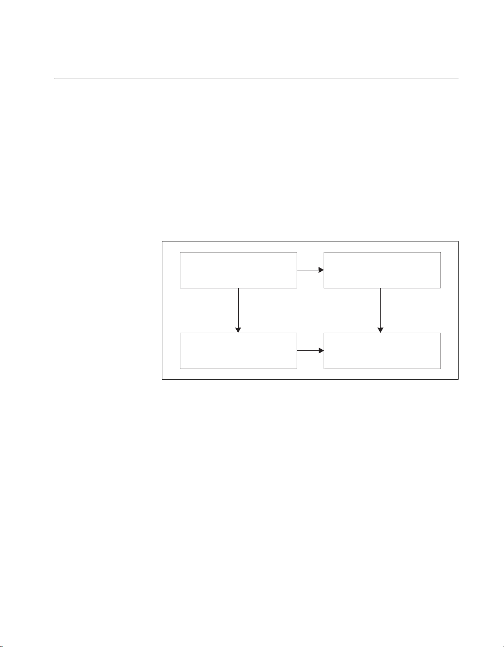
As shown in Figure 1-1, functions are provided to handle four broad tasks:
• Model reduction with additive errors
• Model reduction with multiplicative errors
• Model reduction with frequency weighting of an additive error,
including controller reduction
• Utility functions
Additive Error
Model Reduction
balmoore
redschur
ophank
truncate
balance
mreduce
Multiplicative
Model Reduction
bst
mulhank
Utility Functions
hankelsv
stable
compare
Figure 1-1. MRM Function
Frequency Weighted
Model Reduction
wtbalance
fracred
Xmath Model Reduction Module 1-4 ni.com
Page 12

Chapter 1 Introduction
Certain restrictions regarding minimality and stability are required of the
input data, and are summarized in Table 1-1.
Table 1-1. MRM Restrictions
balance( )
balmoore ( ) A state-space system must be stable and minimal,
A stable, minimal system
having at least one input, output, and state
bst( ) A state-space system must be linear,
continuous-time, and stable, with full rank along
the jω-axis, including infinity
compare( ) Must be a state-space system
fracred( )
hankelsv( ) A system must be linear and stable
mreduce( ) A submatrix of a matrix must be nonsingular
A state-space system must be linear and continuous
for continuous systems, and variant for discrete
systems
mulhank( )
A state-space system must be linear,
continuous-time, stable and square, with full
rank along the jω-axis, including infinity
ophank( )
A state-space system must be linear,
continuous-time and stable, but can be nonminimal
redschur( ) A state-space system must be stable and linear,
but can be nonminimal
stable ( ) No restriction
truncate( )
wtbalance( )
Any full-order state-space system
A state-space system must be linear and
continuous. Interconnection of controller and plant
must be stable, and/or weight must be stable.
Documentation of the individual functions sometimes indicates how the
restrictions can be circumvented. There are a number of model reduction
methods not covered here. These include:
• Padé Approximation
• Methods based on interpolating, or matching at discrete frequencies
© National Instruments Corporation 1-5 Xmath Model Reduction Module
Page 13

Chapter 1 Introduction
Nomenclature
• L2 approximation, in which the L2 norm of impulse response error (or,
by Parseval’s theorem, the L
norm of the transfer-function error along
2
the imaginary axis) serves as the error measure
• Markov parameter or impulse response matching, moment matching,
covariance matching, and combinations of these, for example,
q-COVER approximation
• Controller reduction using canonical interactions, balanced Riccati
equations, and certain balanced controller reduction algorithms
This manual uses standard nomenclature. The user should be familiar with
the following:
• sup denotes supremum, the least upper bound.
• The acute accent (´) denotes matrix transposition.
• A superscripted asterisk (*) denotes matrix transposition and complex
conjugation.
• λ
(A) for a square matrix A denotes the maximum eigenvalue,
max
presuming there are no complex eigenvalues.
•Reλ
(A) and |λi(A)| for a square matrix A denote an arbitrary real part
i
and an arbitrary magnitude of an eigenvalue of A.
Xjω()
• for a transfer function X(·) denotes:
∞
sup
∞– ω∞<<
λ
X*jω()Xjω()[][]
max
12/
• An all-pass transfer-function W(s) is one where for all ω;
Xjω() 1=
to each pole, there corresponds a zero which is the reflection through
the jω-axis of the pole, and there are no jω-axis poles.
• An all-pass transfer-function matrix W(s) is a square matrix where
W′ jω–()Wjω() I=
P >0 and P ≥ 0 for a symmetric or hermitian matrix denote positive
and nonnegative definiteness.
> P2 and P1≥ P2 for symmetric or hermitian P1 and P2 denote
• P
1
P
– P2 is positive definite and nonnegative definite.
1
•A superscripted number sign (#) for a square matrix A denotes the
Moore-Penrose pseudo-inverse of A.
Xmath Model Reduction Module 1-6 ni.com
Page 14

• An inequality or bound is tight if it can be met in practice, for example
1 xx– 0≤log+
is tight because the inequality becomes an equality for x =1. Again,
if F(jω) denotes the Fourier transform of some , the
Heisenberg inequality states,
ft()
-------------------------------------------------------------------------------------------
2
t
ft()2dt
∫
and the bound is tight since it is attained for f(t) = exp + (–kt
∫
12⁄
∫
Commonly Used Concepts
This section outlines some frequently used standard concepts.
Controllability and Observability Grammians
Suppose that G(s)=D + C(sI–A)–1B is a transfer-function matrix with
Reλ
(A)<0. Then there exist symmetric matrices P, Q defined by:
i
2
dt
2
ω
Fjω()2dω
Chapter 1 Introduction
ft() L
∈
2
4π≤
12⁄
2
).
PA′ +AP = –BB′
QA + A′Q = –C′C
These are termed the controllability and observability grammians of the
realization defined by {A,B,C,D}. (Sometimes in the code, WC is used for
P and WO for Q.) They have a number of properties:
• P ≥ 0, with P > 0 if and only if [A,B] is controllable, Q ≥ 0 with Q >0
if and only if [A,C] is observable.
∞
• and
PeAtBB′e
= Qe
∫
• With vec P denoting the column vector formed by stacking column 1
• The controllability grammian can be thought of as measuring the
© National Instruments Corporation 1-7 Xmath Model Reduction Module
0
of P on column 2 on column 3, and so on, and ⊗ denoting Kronecker
product
difficulty of controlling a system. More specifically, if the system is in
the zero state initially, the minimum energy (as measured by the L
norm of u) required to bring it to the state x
eigenvalues of P correspond to systems that are difficult to control,
while zero eigenvalues correspond to uncontrollable systems.
A′ t
dt
IAAI⊗+⊗[]vecP vec(– BB′)=
∞
A′ t
∫
0
C′CeAtdt
0
is x0P –1x0; so small
2
=
Page 15

Chapter 1 Introduction
• The controllability grammian is also E[x(t)x′(t)] when the system
x·Ax Bw+=
noise with .
has been excited from time –∞ by zero mean white
Ewt()w′ s()[]Iδ ts–()=
• The observability grammian can be thought of as measuring the
information contained in the output concerning an initial state.
x·Ax= y, Cx=
If with x(0) = x
∞
y′ t()yt()dt
∫
0
then:
0
=
x′0Qx
0
Systems that are easy to observe correspond to Q with large
eigenvalues, and thus large output energy (when unforced).
lyapunov(A,B*B') produces P and lyapunov(A',C'*C)
•
produces Q.
For a discrete-time G(z)=D + C(zI-A)
–1
B with |λi(A)|<1, P and Q are:
P – APA′ = BB′
Q – A′QA = C′C
The first dot point above remains valid. Also,
∞
k
• and
= QA
PA
∑
k 0=
BB′A ′
k
∞
=
k
∑
k 0=
C′CA′
k
with the sums being finite in case A is nilpotent (which is the case if
the transfer-function matrix has a finite impulse response).
•[I–A⊗ A] vec P = vec (BB′)
lyapunov( ) can be used to evaluate P and Q.
Hankel Singular Values
If P, Q are the controllability and observability grammians of a
transfer-function matrix (in continuous or discrete time), the Hankel
Singular Values are the quantities λ
• All eigenvalues of PQ are nonnegative, and so are the Hankel singular
values.
• The Hankel singular values are independent of the realization used to
calculate them: when A,B,C,D are replaced by TAT
then P and Q are replaced by TPT′ and (T
by TPQT
–1
and the eigenvalues are unaltered.
• The number of nonzero Hankel singular values is the order or
McMillan degree of the transfer-function matrix, or the state
dimension in a minimal realization.
Xmath Model Reduction Module 1-8 ni.com
1/2
(PQ). Notice the following:
i
–1
–1
)′QT–1; then PQ is replaced
, TB, CT
–1
and D,
Page 16

Chapter 1 Introduction
• Suppose the transfer-function matrix corresponds to a discrete-time
system, with state variable dimension n. Then the infinite Hankel
matrix,
2
B
2
B
H
CB CAB CA
CAB CA
=
2
CA
B
has for its singular values the n nonzero Hankel singular values,
together with an infinite number of zero singular values.
The Hankel singular values of a (stable) all pass system (or all pass matrix)
are all 1.
Slightly different procedures are used for calculating the Hankel singular
values (and so-called weighted Hankel singular values) in the various
functions. These procedures are summarized in Table 1-2.
Table 1-2. Calculating Hankel Singular Values
(balance( ))
balmoore( )
hankelsv( )
ophank( )
redschur( )
bst( )
mulhank( )
wtbalance( )
fracred( )
For a discussion of the balancing algorithm, refer to
the Internally Balanced Realizations section; the
Hankel singular values are given by
1/2
diag(R
)=HSV
For a discussion of the balancing algorithm, refer to
the Internally Balanced Realizations section; the
matrix S
diag(SH)
real(sqrt(eig(p*q)))
yields the Hankel singular values through
H
Calls hankelsv( )
Computes a Schur decomposition of P*Q and then
takes the square roots of the diagonal entries
Same as redschur( ) except either P or Q can be
a weighted grammian
© National Instruments Corporation 1-9 Xmath Model Reduction Module
Page 17

Chapter 1 Introduction
Internally Balanced Realizations
Suppose that a realization of a transfer-function matrix has the
controllability and observability grammian property that P = Q = Σ for
some diagonal Σ. Then the realization is termed internally balanced. Notice
that the diagonal entries σ
that is, they are the Hankel singular values. Often the entries of Σ are
assumed ordered with σ
As noted in the discussion of grammians, systems with small (eigenvalues
of) P are hard to control and those with small (eigenvalues of) Q are hard
to observe. Now a state transformation T = α I will cause P = Q to be
replaced by α
expense of difficulty of observation, and conversely. Balanced realizations
are those when ease of control has been balanced against ease of
observation.
Given an arbitrary realization, there are a number of ways of finding a
state-variable coordinate transformation bringing it to balanced form.
A good survey of the available algorithms for balancing is in [LHPW87].
One of these is implemented in the Xmath function
2
P, α–2Q, implying that ease of control can be obtained at the
of Σ are square roots of the eigenvalues of PQ,
i
≥ σ
.
i
i+1
balance( ).
The one implemented in
balmoore( ) as part of this module is more
sophisticated, but more time consuming. It proceeds as follows:
1. Singular value decompositions of P and Q are defined. Because P and
Q are symmetric, this is equivalent to diagonalizing P and Q by
orthogonal transformations.
P=U
Q=UoSo U′
cSc
U′
c
o
2. The matrix,
12⁄
=
HS
0
UHSHV
12⁄
H
is constructed, and from it, a singular value decomposition is obtained:
=
HU
′
HSHVH
3. The balancing transformation is given by:
=
TU
The balanced realization is T
Xmath Model Reduction Module 1-10 ni.com
12⁄–
0S0
–1
AT, T–1B, CT.
UHS
12⁄
H
Page 18

Chapter 1 Introduction
This is almost the algorithm set out in Section II of [LHPW87]. The one
difference (and it is minor) is that in [LHPW87], lower triangular Cholesky
factors of P and Q are used, in place of U
cSc
1/2
and UOS
1/2
in forming H
O
in step 2. The grammians themselves need never be formed, as these
Cholesky factors can be computed directly from A, B, and C in both
continuous and discrete time; this, however, is not done in
balmoore.
The algorithm has the property that:
Thus the diagonal entries of S
The algorithm implemented in
A lower triangular Cholesky factor L
Then the symmetric matrix L
value decomposition), thus L′
the coordinate basis transformation is given by T = L
T′QT = T
Singular Perturbation
A common procedure for approximating systems is the technique of
Singular Perturbation. The underlying heuristic reasoning is as follows.
Suppose there is a system with the property that the unforced responses of
the system contain some modes which decay to zero extremely fast. Then
an approximation to the system behavior may be attained by setting state
variable derivatives associated with these modes to zero, even in the forced
case. The phrase “associated with the modes” is loose: exactly what occurs
is shown below. The phrase “even in the forced case” captures a logical
flaw in the argument: smallness in the unforced case associated with initial
conditions is not identical with smallness in the forced case.
Suppose the system is defined by:
–1
P(T–1)′ = R
T′ QT′ T
1/2
.
1–
PT1–()′ S
==
are the Hankel singular values.
H
balance( ) is older, refer to [Lau80].
of P is found, so that LcLc′ = P.
c
′QLc is diagonalized (through a singular
c
= VRU′, with actually V = U. Finally,
cQLc
H
VR
c
–1/4
, resulting in
·
x
·
x
© National Instruments Corporation 1-11 Xmath Model Reduction Module
A11A
1
A21A
2
y
C
1C2
x
B
1
12
x
22
x
1
x
2
1
u+=
B
2
2
Du+=
(1-1)
Page 19

Chapter 1 Introduction
and also:
Reλ
)<0 and .
i(A22
Reλ
iA11A12A22
–()0<
1–
A
21
Usually, we expect that,
()ReλiA11A12A
Reλ
iA22
–()«
1–
A
22
21
in the sense that the intuitive argument hinges on this, but it is not necessary.
·
Then a singular perturbation is obtained by replacing by zero; this
x
2
means that:
A21x1A22x2B2u++ 0=
or
x
2
1–
A–
A21x1A
22
1–
B2u–=
22
Accordingly,
·
x
A11A12A
1
yC
–()x1DC2A
1C2A22
1–
=()x1B1A12A
A
22
21
1–
A
21
–()u+=
–()u+=
1–
B
22
2
1–
B
22
2
(1-2)
Equation 1-2 may be an approximation for Equation 1-1. This means that:
• The transfer-function matrices may be similar.
• If Equation 1-2 is excited by some u(·), with initial condition x
1(to
), and
if Equation 1-1 is excited by the same u(·) with initial condition given
by,
•x
1(to
then x
) and x2(to) = –A
(·) and y(·) computed from Equation 1-1 and from Equation 1-2
1
–1
A21x1(to)–A
22
–1
22
B2u(to),
should be similar.
• If Equation 1-1 and Equation 1-2 are excited with the same u(·), have
the same x
) and Equation 1-1 has arbitrary x2, then x1(·) and y(·)
1(to
computed from Equation 1-1 and Equation 1-2 should be similar after
a possible initial transient.
As far as the transfer-function matrices are concerned, it can be verified that
they are actually equal at DC.
Xmath Model Reduction Module 1-12 ni.com
Page 20

Chapter 1 Introduction
Similar considerations govern the discrete-time problem, where,
can be approximated by:
mreduce( ) can carry out singular perturbation. For further discussion,
refer to Chapter 2, Additive Error Reduction. If Equation 1-1 is balanced,
singular perturbation is provably attractive.
Spectral Factorization
Let W(s) be a stable transfer-function matrix, and suppose a system S with
transfer-function matrix W(s) is excited by zero mean unit intensity white
noise. Then the output of S is a stationary process with a spectrum Φ(s)
related to W(s) by:
x
k 1+()
1
k 1+()
x
2
A
11A12
A21A
22
x1k()
x
2
x1k()
yk()
x1k 1+()A11A12IA
y
k
C
1C2
x
k()
2
+[]x1k()+=
B
+[]uk()
1A12
C1C2IA
+[]x1k()+=
DC
+[]uk()
–()
IA
–()
–()
22
IA
–()
2
22
22
22
k()
1–
1–
B
1
uk()+=
B
2
Du k()+=
1–
A
21
1–
B
2
A
21
B
2
Φ s() Ws()W′ s–()=
(1-3)
Evidently,
Φ jω() Wjω()W
*
jω()=
so that Φ( jω) is nonnegative hermitian for all ω; when W( jω) is a scalar, so
is Φ( jω) with Φ( jω)=|W( jω)|
2
.
In the matrix case, Φ is singular for some ω only if W does not have full
rank there, and in the scalar case only if W has a zero there.
Spectral factorization, as shown in Example 1-1, seeks a W(jω), given
Φ(jω). In the rational case, a W(jω) exists if and only if Φ(jω) is
© National Instruments Corporation 1-13 Xmath Model Reduction Module
Page 21

Chapter 1 Introduction
nonnegative hermitian for all ω. If Φ is scalar, then Φ(jω)≥0 for all ω.
Normally one restricts attention to Φ(·) with lim
Φ(jω)<∞. A key result
ω→∞
is that, given a rational, nonnegative hermitian Φ(jω) with
lim
Φ(jω)<∞, there exists a rational W(s) where,
ω→∞
• W(∞)<∞.
• W(s) is stable.
• W(s) is minimum phase, that is, the rank of W(s) is constant in Re[s]>0.
In the scalar case, all zeros of W(s) lie in Re[s]≤0, or in Re[s]<0 if Φ(jω)>0
for all ω.
In the matrix case, and if Φ(jω) is nonsingular for some ω, it means that
W(s) is square and W
is nonsingular for all ω.
Moreover, the particular W(s) previously defined is unique, to within right
multiplication by a constant orthogonal matrix. In the scalar case, this
means that W(s) is determined to within a ±1 multiplier.
Example 1-1 Example of Spectral Factorization
Suppose:
Then Equation 1-3 is satisfied by , which is stable and
minimum phase.
Also, Equation 1-3 is satisfied by and , and , and
so forth, but none of these is minimum phase.
bst( ) and mulhank( ) both require execution within the program of
a spectral factorization; the actual algorithm for achieving the spectral
factorization depends on a Riccati equation. The concepts of a spectrum
and spectral factor also underpin aspects of
–1
(s) has all its poles in Re[s]≤ 0, or in Re[s]<0 if Φ(jω)
2
1+
Ws()
s 1–
----------s 2+
ω
---------------=
2
ω
4+
s 1+
-----------
±=
s 2+
s 3–
----------s 2+
wtbalance( ).
s 1–
-----------
s 2+
s 1+
sT–
-----------
e
s 2+
Φ jω()
Xmath Model Reduction Module 1-14 ni.com
Page 22
Chapter 1 Introduction
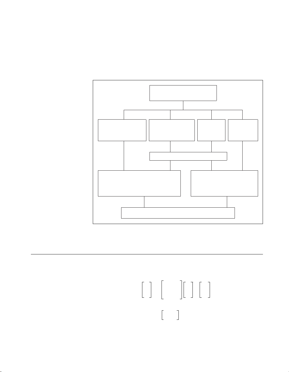
Low Order Controller Design Through Order Reduction
The Model Reduction Module is particularly suitable for achieving low
order controller design for a high order plant. This section explains some of
the broad issues involved.
Most modern controller design methods, for example, LQG and H
∞, yield
controllers of order roughly comparable with that of the plant. It follows
that, to obtain a low order controller using such methods, one must either
follow a high order controller design by a controller reduction step,
or reduce an initially given high order plant model, and then design a
controller using the resulting low order plant, with the understanding that
the controller will actually be used on the high order plant. Refer to
Figure 1-2.
High Order Plant
Plant
Reduction Reduction
Low Order Plant
Figure 1-2. Low Order Controller Design for a High Order Plant
High Order Controller
Controller
Low Order Controller
Generally speaking, in any design procedure, it is better to postpone
approximation to a late step of the procedure: if approximation is done
early, the subsequent steps of the design procedure may have unpredictable
effects on the approximation errors. Hence, the scheme based on high order
controller design followed by reduction is generally to be preferred.
Controller reduction should aim to preserve closed-loop properties as far
as possible. Hence the controller reduction procedures advocated in this
module reflect the plant in some way. This leads to the frequency weighted
reduction schemes of
wtbalance( ) and fracred( ), as described in
Chapter 4, Frequency-Weighted Error Reduction. Plant reduction logically
should also seek to preserve closed-loop properties, and thus should involve
the controller. With the controller unknown however, this is impossible.
Nevertheless, it can be argued, on the basis of the high loop gain property
within the closed-loop bandwidth that is typical of many systems, that
© National Instruments Corporation 1-15 Xmath Model Reduction Module
Page 23

Chapter 1 Introduction
multiplicative reduction, as described in Chapter 4, Frequency-Weighted
Error Reduction, is a sound approach. Chapter 3, Multiplicative Error
Reduction, and Chapter 4, Frequency-Weighted Error Reduction, develop
these arguments more fully.
Xmath Model Reduction Module 1-16 ni.com
Page 24

Additive Error Reduction
This chapter describes additive error reduction including discussions of
truncation of, reduction by, and perturbation of balanced realizations.
Introduction
Additive error reduction focuses on errors of the form,
2
Gjω()G
where G is the originally given transfer function, or model, and G
reduced one. Of course, in discrete-time, one works instead with:
Gejω()Grejω()–
As is argued in later chapters, if one is reducing a plant that will sit inside
a closed loop, or if one is reducing a controller, that again is sitting in a
closed loop, focus on additive error model reduction may not be
appropriate. It is, however, extremely appropriate in considering reducing
the transfer function of a filter. One pertinent application comes specifically
from digital filtering: a great many design algorithms lead to a finite
impulse response (FIR) filter which can have a very large number of
coefficients when poles are close to the unit circle. Model reduction
provides a means to replace an FIR design by a much lower order infinite
impulse response (IIR) design, with close matching of the transfer function
at all frequencies.
jω()–
r
∞
is the
r
∞
© National Instruments Corporation 2-1 Xmath Model Reduction Module
Page 25

Chapter 2 Additive Error Reduction
Truncation of Balanced Realizations
A group of functions can be used to achieve a reduction through truncation
of a balanced realization. This means that if the original system is
·
x
·
x
A11A
1
2
A21A
12
22
x
B
1
1
x
2
u+=
B
2
y
C
1C2
xD
+=
u
(2-1)
and the realization is internally balanced, then a truncation is provided by
·
x
A11x1B1u+=
1
1x1
Du+=
yC
The functions in question are:
• balmoore( )
• balance( ) (refer to the Xmath Help)
• truncate( )
• redschur( )
One only can speak of internally balanced realizations for systems which
are stable; if the aim is to reduce a transfer function matrix G(s) which
contains unstable poles, one must additively decompose it into a stable part
and unstable part, reduce the stable part, and then add the unstable part back
in. The function
stable( ), described in Chapter 5, Utilities, can be used
to decompose G(s). Thus:
G(s) = G
(s) + Gu(s)(Gs(s) stable, Gu(s) unstable)
s
Gsr(s) = found by algorithm (reduction of Gs(s))
(s) = Gsr(s) + Gu(s) (reduction of G(s))
G
r
Xmath Model Reduction Module 2-2 ni.com
Page 26

Chapter 2 Additive Error Reduction
A very attractive feature of the truncation procedure is the availability
of an error bound. More precisely, suppose that the controllability and
observability grammians for [Enn84] are
Σ
0
PQΣ
===
1
0 Σ
2
(2-2)
with the diagonal entries of Σ in decreasing order, that is, σ
≥ σ2 ≥ ···. Then
1
the key result is,
with G, G
Gjω()Grjω()–
the transfer function matrices of Equation 2-1 and Equation 2-2,
r
2trΣ
≤
∞
2
respectively. This formula shows that small singular values can, without
great cost, be thrown away. It also is valid in discrete time, and can be
improved upon if there are repeated Hankel singular values. Provided that
the smallest diagonal entry of Σ
of Σ
, the reduced order system is guaranteed to be stable.
2
strictly exceeds the largest diagonal entry
1
Several other points concerning the error can be made:
• The error G( jω)–G
( jω) as a function of frequency is not flat; it is zero
r
at ω = ∞, and may take its largest value at ω = 0, so that there is in
general no matching of DC gains of the original and reduced system.
• The actual error may be considerably less than the error bound at all
frequencies, so that the error bound formula can be no more than an
advance guide. However, the bound is tight when the dimension
reduction is 1 and the reduction is of a continuous-time
transfer-function matrix.
• With g(·) and g
responses of G and G
(·) denoting the impulse responses for impulse
r
and with Gr of degree k, the following L1 bound
r
holds [GCP88]
gg
–
This bound also will apply for the L
≤
r
1
42k 1+()trΣ
error on the step response.
∞
2
It is helpful to note one situation where reduction is likely to be difficult (so
that Σ will contain few diagonal entries which are, relatively, very small).
Suppose G(s), strictly proper, has degree n and has (n – 1) unstable zeros.
Then as ω runs from zero to infinity, the phase of G(s) will change by
(2n – 1)π/2. Much of this change may occur in the passband. Suppose G
r
(s)
has degree n–1; it can have no more than (n – 2) zeros, since it is strictly
© National Instruments Corporation 2-3 Xmath Model Reduction Module
Page 27

Chapter 2 Additive Error Reduction
proper. So, even if all zeros are unstable, the maximum phase shift when ω
moves from 0 to ∞ is (2n – 3)π/2. It follows that if G(jω) remains large in
magnitude at frequencies when the phase shift has moved past (2n – 3)π/2,
approximation of G by G
approximation may depend somehow on removing roughly cancelling
pole-zeros pairs; when there are no left half plane zeros, there can be no
rough cancellation, and so approximation is unsatisfactory.
As a working rule of thumb, if there are p right half plane zeros in the
passband of a strictly proper G(s), reduction to a G
p + 1 is likely to involve substantial errors. For non-strictly proper G(s),
having p right half plane zeros means that reduction to a G
than p is likely to involve substantial errors.
An all-pass function exemplifies the problem: there are n stable poles and
n unstable zeros. Since all singular values are 1, the error bound formula
indicates for a reduction to order n – 1 (when it is not just a bound, but
exact) a maximum error of 2.
Another situation where poor approximation can arise is when a highly
oscillatory system is to be replaced by a system with a real pole.
will necessarily be poor. Put another way, good
r
(s) of order less than
r
(s) of order less
r
Reduction Through Balanced Realization Truncation
This section briefly describes functions that reduce( ), balance( ),
and
truncate( ) to achieve reduction.
balmoore( )—Computes an internally balanced realization of a
•
system and optionally truncates the realization to form an
approximation.
•
balance( )—Computes an internally balanced realization of a
system.
•
truncate( )—This function truncates a system. It allows
examination of a sequence of different reduced order models formed
from the one balanced realization.
redschur( )—These functions in theory function almost the same
•
as the two features of
state-variable realization of a reduced order model, such that the
transfer function matrix of the model could have resulted by truncating
a balanced realization of the original full order transfer function
matrix. However, the initially given realization of the original transfer
function matrix is never actually balanced, which can be a numerically
hazardous step. Moreover, the state-variable realization of the reduced
Xmath Model Reduction Module 2-4 ni.com
balmoore( ). That is, they produce a
Page 28
Chapter 2 Additive Error Reduction
order model is not one in general obtainable by truncation of an
internally-balanced realization of the full order model.
Figure 2-1 sets out several routes to a reduced-order realization. In
continuous time, a truncation of a balanced realization is again balanced.
This is not the case for discrete time, but otherwise it looks the same.
Full Order Realization
balmoore
(with both steps)
Balanced Realization of
Reduced Order Model
(in continuous time)
Reduced Order Model Transfer Function
balmoore
(with first step)
truncate
balance redschur
Nonbalanced
Realization of
Reduced Order Model
Figure 2-1. Different Approaches for Obtaining the Same Reduced Order Model
Singular Perturbation of Balanced Realization
Singular perturbation of a balanced realization is an attractive way to
produce a reduced order model. Suppose G(s) is defined by,
·
x
·
x
A11A
1
A21A
2
x
B
1
12
x
22
1
u+=
B
2
2
y
© National Instruments Corporation 2-5 Xmath Model Reduction Module
C
1C2
xDu+=
Page 29

Chapter 2 Additive Error Reduction
with controllability and observability grammians given by,
in which the diagonal entries of Σ are in decreasing order, that is,
σ
1≥σ2
the first diagonal entry of Σ
Reλ
defined by:
Σ
0
PQΣ
===
≥ ···, and such that the last diagonal entry of Σ1 exceeds
. It turns out that Reλi( )<0 and
(A11–A
i
1–
A21)< 0, and a reduced order model Gr(s) can be
A
12
22
2
1
0 Σ
2
1–
A
22
x·A11A12A
yC
1C2A22
The attractive feature [LiA89] is that the same error bound holds as for
balanced truncation. For example,
Although the error bounds are the same, the actual frequency pattern of
the errors, and the actual maximum modulus, need not be the same for
reduction to the same order. One crucial difference is that balanced
truncation provides exact matching at ω = ∞, but does not match at DC,
while singular perturbation is exactly the other way round. Perfect
matching at DC can be a substantial advantage, especially if input signals
are known to be band-limited.
Singular perturbation can be achieved with
the two alternative approaches. For both continuous-time and discrete-time
reductions, the end result is a balanced realization.
Hankel Norm Approximation
1–
–()xB1A12– A
–()xDC2A
Gjω()G
A
22
21
1–
A
21
jω()–
r
+()u+=
1–
–()u+=
22
2trΣ
≤
∞
mreduce( ). Figure 2-1 shows
2
1–
B
22
2
B
2
In Hankel norm approximation, one relies on the fact that if one chooses an
approximation to exactly minimize one norm (the Hankel norm) then the
infinity norm will be approximately minimized. The Hankel norm is
defined in the following way. Let G(s) be a (rational) stable transfer
Xmath Model Reduction Module 2-6 ni.com
Page 30

Chapter 2 Additive Error Reduction
ˆ
ˆ
function matrix. Consider the way the associated impulse response maps
inputs defined over (–∞,0] in L
into outputs, and focus on the output over
2
[0,∞). Define the input as u(t) for t <0, and set v(t)=u(–t). Define the
output as y(t) for t > 0. Then the mapping is
∞
yt() CexpAt r+()Bv r()dr
=
∫
0
–1
if G(s)=C(sI-A)
G
norm of G. A key result is that if σ
H
values of G(s), then .
B. The norm of the associated operator is the Hankel
≥ ···, are the Hankel singular
G
σ1=
H
1≥σ2
To avoid minor confusion, suppose that all Hankel singular values of G are
distinct. Then consider approximating G by some stable of prescribed
degree k much that is minimized. It turns out that
ˆ
GG
–
H
G
inf
Gˆof degree k
and there is an algorithm available for obtaining . Further, the
optimum which is minimizing does a reasonable job
of minimizing , because it can be shown that
ˆ
G
ˆ
GG
–
∞
GG
–
where n =deg G, with this bound subject to the proviso that G and are
GG
–
GG
–
ˆ
≤
∞
ˆ
σ
k 1+
G()=
H
G
ˆ
H
σ
j
∑
jk1+=
ˆ
G
allowed to be nonzero and different at s = ∞.
The bound on is one half that applying for balanced truncation.
ˆ
GG
–
However,
• It is actual error that is important in practice (not bounds).
• The Hankel norm approximation does not give zero error at ω = ∞
or at ω = 0. Balanced realization truncation gives zero error at ω = ∞,
and singular perturbation of a balanced realization gives zero error
at ω =0.
There is one further connection between optimum Hankel norm
approximation and L
ˆ
with stable and of degree k and with F unstable, then:
G
error. If one seeks to approximate G by a sum + F,
∞
ˆ
G
ˆ
GG
inf
Gˆof degree k and F unstable
© National Instruments Corporation 2-7 Xmath Model Reduction Module
– F–
σ
k 1+
G()=
∞
Page 31

Chapter 2 Additive Error Reduction
Further, the which is optimal for Hankel norm approximation also is
optimal for this second type of approximation.
ˆ
G
balmoore( )
In Xmath Hankel norm approximation is achieved with
ophank( ).
The most comprehensive reference is [Glo84].
[SysR,HSV,T] = balmoore(Sys,{nsr,bound})
The balmoore( ) function computes an internally-balanced realization of
a continuous system and then optionally truncates it to provide a balance
reduced order system using B.C. Moore’s algorithm.
balmoore( ) is being used to reduce a system, its objective mirrors
When
that of
redschur( ), therefore, if the same Sys and nsr are used for both
algorithms, the reduced order system should have the same transfer
function (though in general the state-variable realizations will be different).
When
balmoore( ) is being used to balance a system, its objective, like
that of balance, is to generate an internally-balanced state-variable
realization. The implementations are not identical.
balmoore( ) only can be applied on systems that have a stable A matrix,
and are controllable and observable, (that is, minimal). Checks, which are
rather time-consuming, are included. The computation is intrinsically not
well-conditioned if
balmoore( ) serves to find a transformation matrix T such that the
Sys is nearly nonminimal. The first part of
controllability and observability grammians after transformation are equal,
and diagonal, with decreasing entries down the diagonal, that is, the system
representation is internally balanced. (The condition number of T is a
measure of the ill-conditioning of the algorithm. If there is a problem with
ill-conditioning,
redschur( ) can be used as an alternative.) If this
common grammian is Σ, then after transformation:
Σ A′
(continuous)
(discrete)
Σ diag σ
1σ2σ3
Singular Values of
Xmath Model Reduction Module 2-8 ni.com
... σns,,,[]= σiσ
Sys. In the second part of balmoore( ), a truncation
+ A Σ = –BB
Σ
– A Σ A
with with the the Hankel
= –BB
i 1+
′Σ
A + A′Σ = –C′C
′Σ
- A
′ Σ
A = –C′C
0>≤σ
i
Page 32

Chapter 2 Additive Error Reduction
s
of the balanced system occurs, (assuming nsr is less than the number of
states). Thus, if the state-space representation of the balanced system is
A
11A12
= B
A21A
22
=
with A
possessing dimension nsr × nsr, B1 possessing nsr rows and C1
11
possessing
A
nsr columns, the reduced order system SysR is:
(continuous) (discrete)
·
x
A11x1B1u+=
1
yC
xDu+=
1
x1k 1+()A11x1k() B1uk()+=
The following error formula is relevant:
(continuous)
CjωIA–()
[]C1jωIA
1–
(discrete)
CejωIA–()
B
1
B
2
yk() C
2 σ
1–
BD+[]C1ejωIA
nsr 1+
C
=
C
1C2
k() Du k()+=
1x1
1–
–()
1
σ
+++[]≤
nsr 2+
B1D+()[]–
–()
... σ
1
∞
ns
1–
B1D+[]–
∞
2 σ
nsr 1+
σ
+++[]≤
nsr 2+
... σ
ns
It is this error bound which is the basis of the determination of the order
of the reduced system when the keyword
bound sought is smaller than , then no reduction is possible which is
2σ
n
consistent with the error bound. If it is larger than , then the constant
bound is specified. If the error
2trΣ
transfer function matrix D achieves the bound.
For continuous systems, the actual approximation error depends on
frequency, but is always zero at ω = ∞. In practice it is often greatest at
ω = 0; if the reduction of state dimension is 1, the error bound is exact, with
the maximum error occurring at DC. The bound also is exact in the special
case of a single-input, single-output transfer function which has poles and
zero alternating along the negative real axis. It is far from exact when the
poles and zeros approximately alternate along the imaginary axis (with the
poles stable).
© National Instruments Corporation 2-9 Xmath Model Reduction Module
Page 33

Chapter 2 Additive Error Reduction
The actual approximation error for discrete systems also depends on
frequency, and can be large at ω = 0. The error bound is almost never tight,
that is, the actual error magnitude as a function of ω almost never attains
the error bound, so that the bound can only be a guide to the selection of the
reduced system dimension.
In principle, the error bound formula for both continuous and discrete
systems can be improved (that is, made tighter or less likely to overestimate
the actual maximum error magnitude) when singular values occur with
multiplicity greater than one. However, because of errors arising in
calculation, it is safer to proceed conservatively (that is, work with the error
bound above) when using the error bound to select
actual error achieved. If this is smaller than required, a smaller dimension
for the reduced order system can be selected.
mreduce( ) provides an alternative reduction procedure for a balanced
realization which achieves the same error bound, but which has zero error
at ω = 0. For continuous systems there is generally some error at ω = ∞,
because the D matrix is normally changed. (This means that normally the
approximation of a strictly proper system through
strictly proper, in contrast to the situation with
systems the D matrix is also normally changed so that, for example, a
system which was strictly causal, or guaranteed to contain a delay (that is,
D = 0), will be approximated by a system
nsr, and examine the
mreduce( ) will not be
balmoore( ).) For discrete
SysR without this property.
The presentation of the Hankel singular values may suggest a logical
σ
dimension for the reduced order system; thus if , it may be
»
kσk 1+
sensible to choose nsr = k.
With
mreduce( ) and a continuous system, the reduced order system
SysR is internally balanced, with the grammian , so
diag σ
...,σ
,,[]
1σ2
nsr
that its Hankel Singular Values are a subset of those of the original system
Sys. Provided , SysR also is controllable, observable, and
stable. This is not guaranteed if , so it is highly advisable to
σ
>
nsrσnsr 1+
σ
nsr
σ
=
nsr 1+
avoid this situation. Refer to the balmoore( ) section for more on the
balmoore( ) algorithm.
With
mreduce( ) and discrete systems, the reduced order system SysR is
not in general balanced (in contrast to
singular values are not in general a subset of those of
>
σ
nsrσsrn 1+
, the reduced order system
observable and stable. This is not guaranteed if , so it is
balmoore( )), and its Hankel
Sys. Provided
SysR also is controllable,
σ
nsr
σ
=
nsr 1+
highly advisable to avoid this situation. For additional information about
the
balmoore( ) function, refer to the Xmath Help.
Xmath Model Reduction Module 2-10 ni.com
Page 34

Related Functions
truncate( )
Chapter 2 Additive Error Reduction
balance(), truncate(), redschur(), mreduce()
SysR = truncate(Sys,nsr,{VD,VA})
The truncate( ) function reduces a system Sys by retaining the first
nsr states and throwing away the rest to form a system SysR.
If for
Sys one has,
Related Functions
A
A
11A12
= B
A21A
22
B
1
=
B
2
C
=
C
1C2
the reduced order system (in both continuous-time and discrete-time cases)
is defined by A
approximation of
well be used after an initial application of
, B1, C1, and D. If Sys is balanced, then SysR is an
11
Sys achieving a certain error bound. truncate( ) may
balmoore( ) to further reduce
a system should a larger approximation error be tolerable. Alternatively, it
may be used after an initial application of
If
Sys was calculated from redschur( ) and VA,VD were posed as
arguments, then
SysR is calculated as in redschur( ) (refer to the
balance( ) or redschur( ).
redschur( ) section).
truncate( ) should be contrasted with mreduce( ), which achieves a
reduction through a singular perturbation calculation. If
Sys is balanced,
the same error bound formulas apply (though not necessarily the same
errors),
truncate( ) always ensures exact matching at s = ∞ (in the
continuous-time case), or exacting matching of the first impulse response
coefficient D (in the discrete-time case), while
matching of DC gains for
Sys and SysR in both the continuous-time and
discrete-time case. For a additional information about the
mreduce( ) ensures
truncate( )
function, refer to the Xmath Help.
balance(), balmoore(), redschur(), mreduce()
© National Instruments Corporation 2-11 Xmath Model Reduction Module
Page 35

Chapter 2 Additive Error Reduction
redschur( )
[SysR,HSV,slbig,srbig,VD,VA] = redschur(Sys,{nsr,bound})
The redschur( ) function uses a Schur method (from Safonov and
Chiang) to calculate a reduced version of a continuous or discrete system
without balancing.
Algorithm
The objective of redschur( ) is the same as that of balmoore( ) when
the latter is being used to reduce a system; this means that if the same
and
the same transfer function matrix. However, in contrast to
redschur( ) do not initially transform Sys to an internally balanced
realization and then truncate it; nor is
there is no balancing offers numerical advantages, especially if
nearly nonminimal.
Sys should be stable, and this is checked by the algorithm. In contrast to
balmoore( ), minimality of Sys (that is, controllability and
observability) is not required.
Sys
nsr are used for both algorithms, the reduced order system should have
balmoore( ),
SysR in balanced form. The fact that
Sys is
If the Hankel singular values of
then those of
SysR in the continuous-time case are .
A restriction of the algorithm is that is required for both
Sys are ordered as ,
σ
>
nsrσnsr 1+
continuous-time and discrete-time cases. Under this restriction,
σ
σ
1σ2
1σ2
... σns0≥≥≥ ≥
... σ
nsr
SysR is
0>≥≥≥
guaranteed to be stable and minimal.
The algorithms depend on the same algorithm, apart from the calculation
of the controllability and observability grammians W
original system. These are obtained as follows:
(continuous)
(discrete)
WcA′ AW
+ BB′–= WoAA′W
c
W
AWcA′– BB′= WoA′WoA– C′C=
c
and Wo of the
c
+ C′C=
o
The maximum order permitted is the number of nonzero eigenvalues of
that are larger than ε.
W
cWo
Xmath Model Reduction Module 2-12 ni.com
Page 36

Chapter 2 Additive Error Reduction
Next, Schur decompositions of WcWo are formed with the eigenvalues of
W
in ascending and descending order. These eigenvalues are the square
cWo
of the Hankel singular values of
Sys, and if Sys is nonminimal, some can
be zero.
The matrices V
V′
AWcWoVA
V′
DWcWoVD
, VD are orthogonal and S
A
S
=
asc
S
=
des
, S
are upper triangular. Next,
asc
des
submatrices are obtained as follows:
V
= V
V
lbig
A
0
I
nsr
rbig
I
=
nsr
V
D
0
and then a singular value decomposition is found:
U
ebigSebigVebig
=
V′
lbigVrbig
From these quantities, the transformation matrices used for calculating
SysR are defined:
S
S
lbig
rbig
V
=
lbigUebigSebig
V
=
rbigVebigSebig
12⁄
12⁄
and the reduced order system is:
′
S
AS
=
A
R
lbig
rbig
B
′
S
lbig
B=
R
A
CS
=
R
rbig
D
An error bound is available. In the continuous-time case it is as follows. Let
G( jω) and G
( jω) be the transfer function matrices of Sys and SysR,
R
respectively.
For the continuous case:
Gjω()G
© National Instruments Corporation 2-13 Xmath Model Reduction Module
jω()–
R
2 σ
∞
nsr 1+
σ
+++()≤
nsr 2+
... σ
ns
Page 37

Chapter 2 Additive Error Reduction
For the discrete-time case:
Related Functions
ophank( )
Gejω()GRejω()–
{bound} is specified, the error bound just enunciated is used to
When
choose the number of states in
is as small as possible. If the desired error bound is smaller than 2σ
2 σ
∞
nsr 1+
SysR so that the bound is satisfied and nsr
σ
+++()≤
nsr 2+
... σ
ns
,
ns
no reduction is made.
In the continuous-time case, the error depends on frequency, but is always
zero at ω = ∞. If the reduction in dimension is 1, or the system
Sys is
single-input, single-output, with alternating poles and zeros on the real
axis, the bound is tight. It is far from tight when the poles and zeros
approximately alternate along the jω-axis. It is not normally tight in the
discrete-time case, and for both continuous-time and discrete-time cases,
it is not tight if there are repeated singular values.
The presentation of the Hankel singular values may suggest a logical
dimension for the reduced order system; thus if , it may be
σkσ
»
k 1+
sensible to choose nsr = k.
ophank(), balmoore()
[SysR,SysU,HSV] = ophank(Sys,{nsr,onepass})
The ophank( ) function calculates an optimal Hankel norm reduction
of
Sys.
Restriction
This function has the following restriction:
• Only continuous systems are accepted; for discrete systems use
makecontinuous( ) before calling bst( ), then discretize the
result.
Sys=ophank(makecontinuous(SysD));
SysD=discretize(Sys);
Xmath Model Reduction Module 2-14 ni.com
Page 38

Algorithm
Chapter 2 Additive Error Reduction
The algorithm does the following. The system Sys and the reduced order
system
SysR are stable; the system SysU has all its poles in Re[s] > 0. If
the transfer function matrices are G(s), G
• G
(s) is a stable approximation of G(s).
r
(s)+Gu(s) is a more accurate, but not stable, approximation of G(s),
• G
r
(s) and Gu(s) then:
r
and optimal in a certain sense.
Of course, the algorithm works with state-space descriptions; that of G(s)
can be minimal, while that of G
(s) cannot be.
r
Behaviors
These statements are explained in the Behaviors section. If
specified, reduction is calculated in one pass. If
set to 0
{onepass=0}, reduction is calculated in (number of states of
onepass is not called or is
onepass is
Sys - nsr) passes. There seems to be no general rule to suggest which
setting produces the more accurate approximation G
. Therefore, if
r
accuracy of approximation for a given order is critical, both should be tried.
As noted previously, if an approximation involving an unstable system is
desired, the default
{onepass=1} is specified.
The following explanation deals first with the keyword {onepass}.
Suppose that σ
, σ2,..., σns are the Hankel Singular values of S, which has
1
transfer function matrix G(s). Suppose that the singular values are ordered
so that:
σ
=== σ
1σ2
Thus, there are n
by n
3
The order
... σ
n
1
equal values, followed by n2– n1 equal values, followed
1
...>σ
n11+
σ
n
m 1–
– n2 equal values, and so forth.
nsr of G
(s) cannot be arbitrary when there are equal Hankel
r
n11+
1+
... σ
σ
n
m 1–
σ
n
2
2+
...>==
n21+
σ
=σns()0≥==>
n
m
singular values. In fact, the orders shown in Table 2-1 for the strictly stable
G
(all poles in Re[s]<0) and strictly unstable Gu (all poles Re[s]>0) are
r
possible (and there are no other possibilities).
© National Instruments Corporation 2-15 Xmath Model Reduction Module
Page 39

Chapter 2 Additive Error Reduction
Table 2-1. Orders of G
Order of
G
nsr
r
0 ns – n
n
1
n
2
Order of
G
nsu
u
1
ns – n
2
ns – n
3
Number of
Eliminated States
(Retaining G
n
n2– n
n3– n
)
u
1
1
2
Number of
Eliminated States
(Discarding G
)
u
ns
ns – n
1
ns – n
2
⇓ ⇓ ⇓ ⇓
n
m –1
0 ns – n
m –1
ns – n
m –1
By abuse of notation, when we say that G is reduced to a certain order, this
corresponds to the order of G
(s) alone; the unstable part of Gu(s) of the
r
approximation is most frequently thrown away. The number of eliminated
states (retaining G
(# of states in G) – (# of states in G
) refers to:
u
) – (# of states in Gu)
r
This number is always the multiplicity of a Hankel singular value. Thus,
is n
when the order of G
the multiplicity of σ
For each order n
i –1
r
n
the number of eliminated states is ni– n
i –1
+ 1 = σni
i – 1
.
of Gr(s), it is possible to find Gr and Gu so that:
i –1
or
Gjω()Grjω()– Gujω()–
(Choosing i = 1 causes G
to be of order zero; identify n0 = 0.) Actually,
r
σ
≤
n
∞
i
among all “approximations” of G(s) with stable part restricted to having
degree n
can never obtain a lower bound on the approximation error than σ
scalar or SISO G(s) case, the G
unique, while in the matrix or MIMO G(s) case, the G
and with no restriction on the degree of the unstable part, one
i –1
(s) which achieves the previous bound is
r
(s) which achieves
r
n
; in the
i
the previous bound may not be unique [Glo84]. The algorithm we use to
find G
(s) and Gu(s) however allows no user choice, and delivers a single
r
pair of transfer function matrices.
The transfer function matrix G
approximation of G( jω). If the D matrix in G
( jω) alone can be regarded as a stable
r
( jω) is approximately
r
chosen, (and the algorithm ensures that it is), then:
Gjω()Grjω()–
Xmath Model Reduction Module 2-16 ni.com
σ
σ
+++≤
n
∞
i
... σ
n
i 1+
ns
(2-3)
Page 40

Chapter 2 Additive Error Reduction
Thus, the penalty for not being allowed to include Gu in the approximation
is an increase in the error bound, by σ
+ ... + σns. A number of
ni + 1
theoretical developments hinge on bounding the Hankel singular values of
G
(s) and Gu(–s) in terms of those of G(s). With Gr(s) of order n
r
i –1
, there
holds:
σ
)σkG()k≤( 12… n
kGr
,, ,=
i 1–
The transfer function matrix G
singular values; however, G
(s), being unstable, does not have Hankel
u
(–s) (which is stable) does have Hankel
u
singular values. They satisfy:
σ
kGu
s–()[]σ
nik+
G()≤
In most cases, the Hankel singular values of G(s) are distinct. If,
accordingly,
GGr– G
then G
has degree (i –1), Gu has degree ns – i and
r
GG
–
σiσ
r
∞
–
+++=
i 1+
σi=
u
∞
... σ
ns
(2-4)
Observe that the bound (Equation 2-3 or Equation 2-4), which is not
necessarily obtained, is one half that applying for both balanced truncation
(as implemented by
also is one half that obtained when applying
realization. In general, the D matrices of G and G
G(∞) ≠ G
G(0) ≠ G
(∞) (in contrast to balmoore( ) and redschur( )). Similarly,
r
(0) in general (in contrast to the result when mreduce is applied
r
balmoore( ) or, effectively, by redschur( )); it
mreduce to a balanced
are different, that is,
r
to a balanced realization). The price paid for obtaining a smaller error
bound overall through Hankel norm reduction is that one no longer
(normally) secures zero error at ω = ∞ or ω = 0.
Two special cases should be noted. If
This constant can be added onto G
approximated by a totally unstable transfer function matrix, with error σ
nsr = 0 then G
(s), so that G(s) is then being
u
(s) is a constant only.
r
1
this type of approximation is known as Nehari approximation. The second
special case arises when
singular value has multiplicity 1). In this case, G
which can then be lumped in with G
© National Instruments Corporation 2-17 Xmath Model Reduction Module
nsr = n
(or NS – 1 if the smallest Hankel
m –1
(s), so that G(s), of degree NS, is then
r
(s) becomes a constant,
u
;
Page 41

Chapter 2 Additive Error Reduction
being approximated by a stable Gr(s) with the actual error (as opposed to
just the error bound) satisfying:
Note G
is optimal, that is, there is no other Gr achieving a lower bound.
r
Onepass Algorithm
Gs() G
s()–
r
σns=
∞
The first steps of the algorithm are to obtain the Hankel singular values of
G(s) (by using
G(s) is checked in this process.) If the user has specified
not coincide with one of 0,n
all the σ
The next step of the algorithm is to calculate the sum G(s)=G
following [SCL90]. (A separate function
hankelsv( )) and identify their multiplicities. (Stability of
nsr and this does
, ... an error message is obtained; generally,
are different, so the occurrence of error messages will be rare.
i
1,n2
(s)+Gu(s),
r
ophred( ) is called for this
purpose.) The controllability and observability grammians P and Q are
found in the usual way.
AP + PA′ = –BB′
QA + A′Q = –C′C
and then a singular value decomposition is obtained of the
matrix :
QP σ
2
I–
n
i
V
U
1U2
SB0
00
′
1
QP σ
′
V
2
2
I–=
n
i
There are precisely n
of σ
. Next, the following definitions are made:
n
i
Xmath Model Reduction Module 2-18 ni.com
– n
zero singular values, this being the multiplicity
i
i –1
12
= σ
22
U1′
U
U1′
U
′
2
′
2
QB=
[]=
A11A
A21A
B
1
B
2
C1C
[]CP V1V
2
2
A′ QAP+()V1V
n
i
2
()
2
Page 42

and finally:
Chapter 2 Additive Error Reduction
#
22
12–A22
12–A22
A
B
2
#
A
21
#
B
2
#
21
G˜s()
A˜S
B˜S
C˜C1C2A
D˜DC2A
1–
B
1–
B
–=
–=
A11A
–()=
B1A
–()=
#
22
These four matrices are the constituents of the system matrix of ,
where:
G˜s() G
s() Gus()+=
r
Digression:
This choice is related to the ideas of [Glo84] in the following way;
in [Glo84], the complete set is identified of satisfying
Gjω()G˜jω()–
˜
G
with having a stable part of order n
G˜s()
σ
=
∞
n
i
. The set is parameterized in
i –1
terms of a stable transfer function matrix K(s) which has to satisfy
2
2
′
Ks()B
+ 0=
C
IK′ jω–()Kjω()– 0forallω≤
with C
of [Glo84], and enjoying the property . The particular
, B2 being two matrices appearing in the course of the algorithm
2
′
C
C2B2B
2
′
=
2
choice
Ks() C
–=
()
2C′2C2
#
B
2
in the algorithm of [Glo84] and flagged in corollary 7.3 of [Glo84] is
equivalent to the previous construction, in the sense of yielding the
˜
same , though the actual formulas used here and in [Glo84] for the
G
s
construction procedure are quite different. In a number of situations,
including the case of scalar (SISO)G(s), this is the only choice.
The next step of the algorithm is to call
its stable and unstable parts, call them and ,
always assign the matrix to , and the final step of the algorithm is
© National Instruments Corporation 2-19 Xmath Model Reduction Module
D˜G
˜
stable( ), to separate into
˜
stable( ) will
s()
G˜s()
s()
r
G
u
G˜s()
Page 43

Chapter 2 Additive Error Reduction
to choose the D matrix of Gr(s), by splitting between Gr(s) and Gu(s).
This is done by using a separate function
the unstable output of
multipass Hankel reduction algorithm, described further below, K(s) is
reduced to the constant K
that is, if it is larger than,
then one chooses:
stable( ), and let K(s)=G
(the approximation), which satisfies,
0
Ks() K
–
G
u
σ1K() ... σσ
0
∞
σ≤
ni1+
s–()K0–
∞
GrG
G
G
u
G() ... σ
≤
˜
r
˜
u
˜
D
ophiter( ). Suppose G
(–s). By applying the
u
K()++≤
nsni–
G()++
n
s
n
s
σkG()
∑
kni1+=
K0+=
K0+=
(s) is
u
This ensures satisfaction of the error bound for G – G
given previously,
r
because:
˜
˜
GG
–
r
GG
=
∞
= KK
σ
r
˜
GG
G() σ
n
i
–– G
––
r
G
u
˜
G
u
ni1+
˜
K0–()+
u
–
+
∞
G() ... σ
∞
0
∞
G()+++≤
n
s
Multipass Algorithm
We now explain the multipass algorithm. For simplicity in first explaining
the idea, suppose that the Hankel singular values at every stage or pass are
distinct.
1. Find a stable order ns – 1 approximation G
Gjω()G
ns 1–
jω–
∞
(This can be achieved by the algorithm already given, and there is no
unstable part of the approximation.)
Xmath Model Reduction Module 2-20 ni.com
(s) of G(s) with:
n–1
σnsG()=
Page 44

Chapter 2 Additive Error Reduction
2. Find a stable order ns – 2 approximation G
G
ns 1–
jω()G
ns 2–
jω()–
∞
of G
ns –2
σ
()=
ns 1–Gns 1–
ns –1
(s), with
.
.
.
3. (Step ns–nr):
Find a stable order nsr approximation of G
with
G
Then, because for ,
isi–≤
for , ..., this being a property of the algorithm, there follows:
jω()G
nsr 1+
σiG
Gjω()G
jω()–
nsr
()σ
ns 1–
σ
iGns 2–
jω()– σ
nsr
∞
G()≤ ins<
i
()σiG
nsr 1+Gnsr 1+
ns
≤
∑
insr1+=
σ
nsr 1+Gnsr 1+
()≤
ns 1–
()... σ
σiG()
nsr +1
()=
++ G()≤
,
ns
The only difference that arises when singular values have multiplicity in
excess of 1 is that the degree reduction at a given step is greater. Thus, if
σ
(G) has multiplicity k, then G(s) is approximated by G
ns
(s) of degree
ns – k
ns – k.
No separate optimization of the D matrix of G
is required. The
nsr
approximation error bound is the same as for the first algorithm. The actual
approximation error may be different. Notice that this second algorithm
does not calculate an unstable G
Gjω()G
nsr
u
jω()– Gujω()–
(s) such that
σ
=
nsr 1+
∞
Discrete-Time Systems
No special algorithm is presented for discrete-time systems. Any stable
discrete-time transfer-function matrix G(z) can be used to define a stable
continuous-time transfer-function matrix by a bilinear transformation, thus
α s+
------------
=
Hs() G
when α is a positive constant.
© National Instruments Corporation 2-21 Xmath Model Reduction Module
α s–
Page 45

Chapter 2 Additive Error Reduction
We use sysZ to denote G(z) and define:
bilinsys=makepoly([-1,a]/makepoly([1,a])
as the mapping from the z-domain to the s-domain. The specification is
reversed because this function uses backward polynomial rotation. Hankel
norm reduction is then applied to H(s), to generate, a stable reduced order
approximation H
(s) and unstable Hu(s) such that:
r
HH
–– σi=
rHu
HH
– σiσ
r
+++=
ni1+
... σ
ns
Here, the s
the same:
We then implement the s-domain equivalent with:
sysS=subsys(sysZ,bilinsys)
There is no simple rule for choosing α; the choice α = 1 is probably as good
as any. The orders of G
respectively. The error formulas are as follows:
Impulse Response Error
If Gr is determined by the first (single-pass) algorithm, the impulse
response error (for t > 0) between the impulse responses of G and G
be bounded. As shown in Corollary 9.9 of [Glo84], if G
and the multiplicity of the ith larger singular value σ
are the Hankel singular values of both G(z) and H(s); they are
ni
z 1–
-----------
z 1+
z 1–
-----------
z 1+
σ
=
∞
n
i
++≤
∞σn
i
σ
of G is r, then:
i
...σ
ni1+
is of degree i –1
r
ns
r
jω
Ge
()Grejω()– Guejω()–
Grz() Hrα
=
=
z() Huα
G
u
and Gu are the same as those of Hr and Hu,
r
Gejω()Grejω()–
can
σjGG
–[]σ
σ
ji– 1+
Xmath Model Reduction Module 2-22 ni.com
r
G for j≤ 1 2 ... 2i 2 r+–,, ,=
i
G()for j≤ 2 i 1– r ..., ns i 1–+,+=
Page 46

Chapter 2 Additive Error Reduction
It follows by a result of [BoD87] that the impulse response error for t >0
satisfies:
ns
gt() grt()– 122i 2– r+()σ
Evidently, Hankel norm approximation ensures some form of
approximation of the impulse response too.
Unstable System Approximation
A transfer function G(s) with stable and unstable poles can be reduced by
applying
stable( ) to separate G(s) into a stable and unstable part. The
former is reduced and then the unstable part can be added back on. For
additional information about the
Help.
Related Functions
stable(), redschur(), balmoore()
G() σjG()
+≤
i
∑
ir+
ophank( ) function, refer to the Xmath
© National Instruments Corporation 2-23 Xmath Model Reduction Module
Page 47

Multiplicative Error Reduction
ˆ
This chapter describes multiplicative error reduction presenting
two reasons to consider multiplicative rather than additive error reduction,
one general and one specific.
Selecting Multiplicative Error Reduction
The general reason to use multiplicative error reduction is that many
specifications are given using decibels; ±1 db corresponds to a
multiplicative error of about 12%. Specifications regarding phase shift also
can be regarded as multiplicative error statements: ±0.05 radians of phase
shift is like 5% multiplicative error also.
The more specific reason arises in considering the problem of plant
approximation, with a high order (possibly very high order) plant being
initially prescribed, with no controller having been designed, and with a
requirement to provide a simpler model of the plant, possibly to allow
controller design. Consider the arrangement of Figure 3-1, controller C(s)
designed for G(s)j with G(s) = (I + ∆)G(s).
3
∆
CG
Figure 3-1. Controller C(s) Designed for Multiplicative Error Reduction
The full order plant is G = (I + ∆)G, and the reduced order model is .
Since , this means that ∆ is the multiplicative error.
Another way one could measure the multiplicative error would be as
GG
–()G
product gives two more possibilities again.
The following multiplicative robustness result can be found in [Vid85].
© National Instruments Corporation 3-1 Xmath Model Reduction Module
ˆ
GG
ˆ
ˆ
–()G
1–
ˆ
. In the matrix plant case, interchange of the order of the
ˆ
1–
∆=
G
Page 48

Chapter 3 Multiplicative Error Reduction
ˆ
ˆ
Multiplicative Robustness Result
Suppose C stabilizes , that has no jω-axis poles, and
that G has the same number of poles in Re[s] ≥ 0 as . If for all ω,
∆ jω()Gˆjω()Cjω()IGˆjω()Cjω()+[]
then C stabilizes G.
This result indicates that if a controller C is designed to stabilize a nominal
or reduced order model , satisfaction of Equation 3-1 ensures that the
controller also will stabilize the true plant G.
In reducing a model of the plant, there will be concern not just to have this
type of stability property, but also concern to have as little error as possible
between the designed system (based on ) and the true system (based
on G). Extrapolation of the stability result then suggests that the goal
should be not just to have Equation 3-1, but to minimize the quantity on the
left side of Equation 3-1, or its greatest value:
max ∆ jω()Gˆjω()Cjω()IGˆjω()Cjω()+[]
ω
However, there are difficulties. The principal one is that if we are reducing
the plant without knowledge of the controller, we cannot calculate the
measure because we do not know C(jω). Nevertheless, one could presume
that, for a well designed system, will be close to I over the
operating bandwidth of the system, and have smaller norm than 1 (tending
to zero as ω→∞ in fact) outside the operating bandwidth of the system.
This suggests that in the absence of knowledge of C, one should carry out
multiplicative approximation by seeking to minimize:
ˆ
G
∆ GG
–()G
=
1–
ˆ
ˆ
ˆ
G
1–
1<
(3-1)
G
G
{}
GˆCI GˆC+()
1–
1–
max ∆ jω() ∆jω()
ω
=
∞
This is the prime rationale for (unweighted) multiplicative reduction of a
plant.
Two other points should be noted. First, because frequencies well beyond
the closed-loop bandwidth, will be small, it is in a sense,
GˆCI GˆC+()
1–
wasteful to seek to have ∆(jω) small at very high frequencies. The choice
of as the index is convenient, because it removes a
maxω∆ jω()
requirement to make assumptions about the controller, but at the same time
it does not allow to be made even smaller in the closed-loop
Xmath Model Reduction Module 3-2 ni.com
∆ jω()
Page 49

Chapter 3 Multiplicative Error Reduction
bandwidth at the expense of being larger outside this bandwidth, which
would be preferable.
–()G
ˆ
Second, the previously used multiplicative error is . In the
algorithms that follow, the error appears. It is easy to
δ GG
=
ˆ
–()G
ˆ
GG
1–
1–
ˆ
check that:
∆ jω()
δ jω()
-------------------------------
≤
∞
1 ∆ jω()
–
∞
∞
and
δ jω()
∆ jω()
-------------------------------
≤
∞
1 δ j ω()
–
∞
∞
This means that if either bound is small, so is the other, with the bounds
approximately equal.
bst( )
Two algorithms for multiplicative reduction are presented:
a mnemonic for balanced stochastic truncation, and
Roughly, they relate to one another in the same way that
and
ophank( ) relate, that is, one focuses on balanced realization
bst( ),
mulhank( ).
redschur( )
truncation and the other on Hankel norm approximation. Some of the
similarities and differences are as follows:
• When the errors are small, the error bound formula for
about one half of that for
• With
bst( ), the actual multiplicative error as a function of frequency
bst( ).
bst( ) is
goes to zero as ω→∞ (or, after using an optional transformation given
in the algorithm description, to zero as ω→ 0); with
mulhank( ), the
error tends to be more uniform as a function of frequency.
bst( ) can handle nonsquare reduction, while mulhank( ) cannot.
•
• Both algorithms are restricted to stable G(s); both preserve right half
plane zeros, that is, these zeros are copied into the reduced order
object; both have difficulties with jω-axis zeros of G(s), but these
difficulties are not insuperable.
[SysR,HSV] = bst(Sys,{nsr,left,right,bound,method})
The bst( ) function calculates a balanced stochastic truncation of Sys for
the multiplicative case.
© National Instruments Corporation 3-3 Xmath Model Reduction Module
Page 50

Chapter 3 Multiplicative Error Reduction
∞
ω
The objective of the algorithm is to approximate a high-order stable transfer
function matrix G(s) by a lower-order G
(g-gr)inv(g) minimized, under the condition that G
prescribed order.
Restrictions
This function has the following restrictions:
• The user must ensure that the input system is stable and nonsingular at
s = infinity.
• The algorithm may be problematic if the input system has a zero on the
jω-axis.
• Only continuous systems are accepted; for discrete systems use
makecontinuous( ) before calling bst( ), then discretize the
result.
Sys=bst(makecontinuous(SysD));
SysD=discretize(Sys);
Algorithm
The modifications described in this section allow you to circumvent the
previous restrictions.
(s) with either inv(g)(g-gr) or
r
is stable and of the
r
The objective of the algorithm is to approximate a high order stable transfer
function matrix G(s) by a lower order G
either or
GG
–()G
under the constraint that G
1–
r
G1–GG
∞
is stable and of prescribed order nsr. In case
r
(s) with, in the square G(s) case,
r
–()
(approximately) minimized,
r
G is not square but has full row rank, the algorithm seeks to minimize:
GG
–()
GG*()1–GG
r
*
Recall that so that when ,
X*s() X′ s–()= sj
X
jω() X*jω()=
*
–()
r
∞
=
When G is not square but has full column rank, the algorithm seeks to
minimize:
–()G*G()1–GG
GG
r
Xmath Model Reduction Module 3-4 ni.com
–()
r
* ∞
Page 51

Chapter 3 Multiplicative Error Reduction
These cases are secured with the keywords right and left, respectively.
If the wrong option is requested for a nonsquare G(s), an error message will
result.
The algorithm has the property that right half plane zeros of G(s) remain as
right half plane zeros of G
zeros in Re[s] > 0, G
n
zeros in Re[s] > 0 it would not be proper, [Gre88].
+
(s). This means that if G(s) has order nsr with n+
r
(s) must have degree at least n+, else, given that it has
r
The conceptual basis of the algorithm can best be grasped by considering
the case of scalar G(s) of degree n. Then one can form a minimum phase,
stable W(s) with |W(jω)|
function) W
–1
(–s) G(s). This all pass function has a mixture of stable and
2
= |G(jω)|2 and then an all-pass function (the phase
unstable poles, and it encodes the phase of G(jω). Its stable part has n
Hankel singular values σ
with σi ≤ 1, and the number of σi equal to 1 is the
i
same as the number of zeros of G(s) in Re[s] > 0. State-variable realizations
of W,G and the stable part of W
and when the stable part of W
–1
(–s)G(s) can be connected in a nice way,
–1
(–s)G(s) has a balanced realization, we say
that the realization of G is stochastically balanced. Truncating the balanced
realization of the stable part of W
–1
(–s)G(s) induces a corresponding
truncation in the realization of G(s), and the truncated realization defines an
approximation of G. Further, a good approximation of a transfer function
encoding the phase of G somehow ensures a good approximation, albeit in
a multiplicative sense, of G itself.
Algorithm with the Keywords right and left
The following description of the algorithm with the keyword right is
based on ideas of [GrA86] developed in [SaC88]. The procedure is almost
the same when
algorithm finds an approximation in the same manner as for
transposes the approximation to yield the desired G
1. The algorithm checks
• That the system is state-space, continuous, and stable
• That a correct option has been specified if the plant is nonsquare
• That D is nonsingular; if the plant is nonsquare, DD´ must be
© National Instruments Corporation 3-5 Xmath Model Reduction Module
left is specified, except the transpose of G(s) is used; the
(s).
r
nonsingular
right, but
Page 52

Chapter 3 Multiplicative Error Reduction
2. With G(s)=D + C(sI – A)–1B and stable, with DD´ nonsingular and
G(jω) G'(–jω) nonsingular for all ω, part of a state variable realization
of a minimum phase stable W(s) is determined such that
W´(–s)W(s) = G(s)G´(–s) with
Ws() D
+=
WCW
sI Aw–()
1–
B
W
The state variable matrices in W(s) are obtained as follows. The
controllability grammian P associated with G(s) is first found from
AP + PA´ +BB´=0 then A
=A, BW=PC´+BD´.
W
When G(s) is square, the algorithm checks to see if there is a zero or
singularity of G(s) close to the jω-axis (the zeros are given by the
eigenvalues of A – BD
schur( )). If one is found, you are warned that results may be
–1
C and are computed reliably with the aid of
unreliable. Next, a stabilizing solution Q is found for the following
Riccati equation:
′
QA A
The
singriccati( ) function is used; failure of the nonsingularity
QCB′WQ–()′DD′()1–CB
′
W
Q–()++ 0=
condition on G(jω)G´(–jω) will normally result in an error message
that no stabilizing solution exists. To obtain the best numerical results,
singriccati( ) is invoked with the keyword {method="schur"}.
Although D
, CW are not needed for the remainder of the algorithm,
W
they are simply determined in the square case by
D′C
D
W
D1–CB
W
′
Q–()==
W
with minor modification in the nonsquare case. The real point of the
algorithm is to compute P and Q; the matrix Q satisfies (square or
nonsquare case).
QA A
QC
C
++ 0=
W
W
′
′
P, Q are the controllability and observability grammians of the transfer
function C
the strictly proper, stable part of θ(s)=W
(sI – A)–1B. This transfer function matrix, it turns out, is
W
–T
(–s)G(s), which obeys the
matrix all-pass property θ(s)θ´(–s)=I, and is the phase matrix
associated with G(s).
3. Compute ordered Schur decompositions of PQ, with the eigenvalues
of PQ is ascending and descending order. Obtain the phase matrix
Hankel singular values, that is, the Hankel singular values of the
Xmath Model Reduction Module 3-6 ni.com
Page 53

Chapter 3 Multiplicative Error Reduction
strictly proper stable part of θ(s), as the square roots of the eigenvalues
of PQ. Call these quantities ν
. The Schur decompositions are,
i
where V
′
V
PQVAS
A
, VD are orthogonal and S
A
= V
asc
′
PQVDS
D
, S
asc
=
are upper triangular.
des
des
4. Define submatrices as follows, assuming the dimension of the reduced
order system
nsr is known:
V
V
= V
lbig
A
0
I
nsr
rbig
I
=
nsr
V
D
0
Determine a singular value decomposition,
U
ebigSebigVebig
′
V
V
=
lbig
rbig
and then define transformation matrices:
S
=
lbig
S
rbig
The reduced order system G
A
′
S
AS
=
R
lbig
rbig
V
lbigUebigSebig
V
=
rbigVebigSebig
is:
r
12⁄–
12⁄–
′
S
B
R
lbig
B=
A
CS
=
CS
=
R
R
rbig
rbig
where step 4 is identical with that used in
the matrices P, Q which determine V
controllability and observability grammians of C
than of C(sI – A)
–1
B, the controllability grammian of G(s) and the
D
D=A
R
redschur( ), except
, VD and so forth, are the
A
(sI – A)–1B rather
W
observability grammian of W(s).
The error formula [WaS90] is:
1–
GG
–()∞2
G
obey νi ≤ 1. One can only eliminate νi where νi < 1. Hence, if nsr is
All ν
i
chosen so that ν
algorithm also checks that
© National Instruments Corporation 3-7 Xmath Model Reduction Module
= 1, the algorithm produces an error message. The
nsr + 1
nsr does not exceed the dimension of a minimal
≤
r
∑
v
i
-------------
1 vi–
(3-2)
Page 54

Chapter 3 Multiplicative Error Reduction
state-variable representation of G. In this case, the user is effectively asking
for G
= G. When the phase matrix has repeated Hankel singular values,
r
they must all be included or all excluded from the model, that is,
ν
= ν
nsr
is not permitted; the algorithm checks for this.
nsr + 1
The number of ν
as mentioned already, these zeros remain as zeros of G
If
error is specified, then the error bound formula (Equation 3-2) in
conjunction with the ν
For nonsquare G with more columns than rows, the error formula is:
If the user is presented with the ν
intelligently choosing
be tight, except when nsr = ns –1.
Securing Zero Error at DC
The error G–1(G – Gr) as a function of frequency is always zero at ω = ∞.
When the algorithm is being used to approximate a high order plant by a
low order plant, it may be preferable to secure zero error at ω = 0. A method
for doing this is discussed in [GrA90]; for our purposes:
1. We need a bilinear transformation of sys = 1/z. Given G(s) we generate
H(s) through:
bilinsys=makepoly([b3,b4]/makepoly([b1,b2])
sys=subsys(sys,bilinsys)
2. Reduce with the previous algorithm:
[sr,nsr,hsv] = bst(sys)
3. Use the bilinear transformation s = 1/z again:
[sr1,nsr1] = bilinear(sr,nsr,[0,1,1,0])
equal to 1 is the number of zeros in Re[s]>0 of G(s), and
i
(s).
r
values from step 3 is used to define nsr for step 4.
i
ns
v
2
≤
∑
insr1+=
i
-------------
1 vi–
GG
–()
r
*
nsr. However, the error bound is not guaranteed to
G*G()1–GG
–()
r
, the error formula provides a basis for
i
12⁄
∞
The νi are the same for G(s) and H(s)=G(s–1). The error bound formula is
the same; H is stable and H( jω)H'(–jω) of full rank for all ω including
ω = ∞ if and only if G has the same property; right half plane zeros of G are
still preserved by the algorithm. The error G
–1
(G – Gr), though now zero at
ω = 0, is in general nonzero at ω = ∞.
Xmath Model Reduction Module 3-8 ni.com
Page 55

Chapter 3 Multiplicative Error Reduction
∞
∞
Hankel Singular Values of Phase Matrix of G
The νi, i = 1,2,...,ns have been termed above the Hankel singular values of
the phase matrix associated with G. The corresponding quantities for G
ν
, i = 1,..., nsr.
i
Further Error Bounds
The introduction to this chapter emphasized the importance of the error
measures
GG
–()G
1–
r
r
for plant reduction, as opposed to or
The BST algorithm ensures that in addition to (Equation 3-2), there holds
[WaS90a].
which also means that for a scalar system,
1–
or
G
GG
–()
G
20log
r
r
1–
GG
–()∞2
G
r
------
10
G
r
r
8.69≤ 2
r
1–
G1–GG
GG
–()G
r
ns
v
i
ns
∑
∑
-------------
1 vi–
v
i
-------------
1 vi–
≤
insr1+=
insr1+=
–()
dB
are
r
r
∞
and, if the bound is small:
ns
v
i
phase G() phase Gr()–
insr1+=
∑
-------------
1 vi–
radians≤
Reduction of Minimum Phase, Unstable G
For square minimum phase but not necessarily stable G, it also is possible
to use this algorithm (with minor modification) to try to minimize (for G
of a certain order) the error bound
GG
–()G
r
r1–∞
© National Instruments Corporation 3-9 Xmath Model Reduction Module
r
Page 56

Chapter 3 Multiplicative Error Reduction
which also can be relevant in finding a reduced order model of a plant.
The procedure requires G again to be nonsingular at ω = ∞, and to have no
jω-axis poles. It is as follows:
1. Form H = G
then H is described by A – BD
stable, and of full rank on the jω-axis.
2. Form H
3. Set G
Observe that
–1
. If G is described by state-variable matrices A, B, C, D,
of the desired order to minimize approximately:
r
–1
= H
.
r
r
H1–HH
–1
C, BD–1, –D–1C, D–1. H is square,
1–
H
HH
–()
r
∞
–()IH1–H
r
IGG
=
G
–=
–=
r
G–()G
r
r
1–
1–
r
The reduced order G
will have the same poles in Re[s]>0 as G, and
r
be minimum phase.
Imaginary Axis Zeros (Including Zeros at ∞)
We shall now explain how to handle the reduction of G(s) which has a rank
drop at s = ∞ or on the jω-axis. The key is to use a bilinear transformation,
[Saf87]. Consider the bilinear map defined by
s
-------------------=
z
---------------=
bs 1+
–1
where 0 < a < b
and mapping G(s) into through:
G˜s() G
=
Gs() G
=
za–
bz– 1+
sa+
G˜s()
sa–
-------------------
bs– 1+
sa+
˜
---------------
bs 1+
Xmath Model Reduction Module 3-10 ni.com
Page 57

Chapter 3 Multiplicative Error Reduction
The values of G(s), as shown in Figure 3-2, along the jω-axis are
the same as the values of around a circle with diameter defined by
[a – j0, b
–1
+ j0] on the positive real axis.
G˜s()
a
1–
b
Gs()
G˜s()
valuesvalues
Figure 3-2. Bilinear Mapping from G(s) to (Case 1)
Also, the values of , as shown in Figure 3-3, along the jω-axis are
G˜s()
G˜s()
the same as the values of G(s) around a circle with diameter defined by
–1
[–b
+ j0, –a + j0].
1–
b
Gs()
-a
G˜s()
valuesvalues
Figure 3-3. Bilinear Mapping from G(s) to (Case 2)
G˜s()
We can implement an arbitrary bilinear transform using the subsys( )
function, which substitutes a given transfer function for the s- or z-domain
operator.
sa–
-------------------
To implement use:
gtildesys=subsys(gsys,makep([-b,1]/makep([1,-a])
To implement use:
gsys=subsys(gtildesys,makep([b,1]/makep([1,a])
=
G˜s() G
=
Gs() G
bs– 1+
sa+
˜
-----------
s 1+
Note
The systems substituted in the previous calls to subsys invert the function
specification because these functions use backward polynomial rotation.
© National Instruments Corporation 3-11 Xmath Model Reduction Module
Page 58

Chapter 3 Multiplicative Error Reduction
Any zero (or rank reduction) on the jω-axis of G(s) becomes a zero (or rank
reduction) in Re[s] > 0 of , and if G(s) has a zero (or rank reduction)
at infinity, this is shifted to a zero (or rank reduction) of at the point
–1
b
, (in Re[s] > 0). If all poles of G(s) are inside the circle of diameter
–1
[–b
+ j0, a + j0], all poles of will be in Re[s] < 0, and if G(s) has no
zero (or rank reduction) on this circle, will have no zero (or rank
reduction) on the jω-axis, including ω = ∞.
G˜s()
G˜s()
G˜s()
G˜s()
If G(s) is nonsingular for almost all values of s, it will be nonsingular or
have no zero or rank reduction on the circle of diameter [–b
–1
+ j0, –a + j 0]
for almost all choices of a,b. If a and b are chosen small enough, G(s) will
have all its poles inside this circle and no zero or rank reduction on it, while
G˜s()
then will have all poles in Re[s] < 0 and no zero or rank reduction on
the jω-axis, including s = ∞. The steps of the algorithm, when G(s) has a
zero on the jω-axis or at s = ∞, are as follows:
1. For small a,b with 0 < a < b
gtildesys.
2. Reduce to , this being possible because is stable and
G˜s() G
˜
r
–1
s() G˜s()
G˜s() G
, form as shown for
=
sa–
-------------------
bs– 1+
has full rank on s = jω, including ω = ∞.
G
3. Form as shown for
The error will be overbounded by the error
1–
˜
G
G˜G
s() G
r
1–
G
GG
r
, and G
∞
–()
˜
–()
r
bs 1+
r
∞
will contain the same zeros in Re[s] ≥ 0 as G.
r
gsys.
sa+
˜
---------------
=
If there is no zero (or rank reduction) of G(s) at the origin, one can take
–1
a =0 and b
needed, and at the very least b
lie in the circle of diameter [–b
= bandwidth over which a good approximation of G(s) is
–1
sufficiently large that the poles of G(s)
–1
+ j0, –a + j 0]. If there is a zero or rank
reduction at the origin, one can replace a =0 by a = b. It is possible to take
b too small, or, if there is a zero at the origin, to take a too small. The user
will be presented with an error message that there is a jω-axis zero and/or
that the Riccati equation solution may be in error. The basic explanation is
that as b → 0, and thus a → 0, the zeros of approach those of G(s).
Thus, for sufficiently small b, one or more zeros of may be identified
G˜s()
˜
s()
G
as lying on the imaginary axis. The remedy is to increase a and/or b above
the desirable values.
The procedure for handling jω-axis zeros or zeros at infinity will be
deficient if the number of such zeros is the same as the order of G(s)—for
example, if G(s) = 1/d(s), for some stable d(s). In this case, it is possible
Xmath Model Reduction Module 3-12 ni.com
Page 59

Chapter 3 Multiplicative Error Reduction
again with a bilinear transformation to secure multiplicative
approximations over a limited frequency band. Suppose that
s
G˜s() G
--------------
=
εs 1+
Create a system that corresponds to with:
gtildesys=subs(gsys,(makep([-eps,1])/makep([1,-]))
bilinsys=makep([eps,1])/makep([1,0])
sys=subsys(sys,bilinsys)
G˜s()
Under this transformation:
•Values of G(s) along the jω-axis correspond to values of around
a circle in the left half plane on diameter (–ε
• Values of along the jω-axis correspond to values of G(s) around
G˜s()
a circle in the right half plane on diameter (0, ε
Multiplicative approximation of (along the jω-axis) corresponds to
G˜s()
–1
+ j0, 0).
–1
G˜s()
+ j0).
multiplicative approximation of G(s) around a circle in the right half plane,
touching the jω-axis at the origin. For those points on the jω-axis near the
circle, there will be good multiplicative approximation of G( jω). If it is
desired to have a good approximation of G(s) over an interval [–jΩ, jΩ],
then a choice such as ε
–1
= 5 Ω or 10 Ω needs to be made. Reduction then
proceeds as follows:
1. Form .
2. Reduce through
3. Form with:
G˜s()
G˜s()
G
s() G
r
gsys=subsys(gtildesys(gtildesys,
makep([-eps,-1])/makep[-1,-0]))
˜
r
bst( ).
s 1 εs–()⁄()–=
Notice that the number of zeros of G(s) in the circle of diameter
1–
, j0+()s
0 ε
sets a lower bound on the degree of G
plane zeros of , and must be preserved by
G˜s()
(s)—for such zeros become right half
r
bst( ). Obviously, zeros at
s = ∞ are never in this circle, so a procedure for reducing G(s) = 1/d(s) is
available.
© National Instruments Corporation 3-13 Xmath Model Reduction Module
Page 60

Chapter 3 Multiplicative Error Reduction
There is one potential source of failure of the algorithm. Because G(s) is
stable, certainly will be, as its poles will be in the left half plane circle
on diameter . If acquires a pole outside this circle
(but still in the left half plane of course)—and this appears possible in
principle—G
be encountered, a smaller value of ε should be used.
Related Functions
redschur(), mulhank()
mulhank( )
[SysR,HSV] = mulhank(Sys,{nsr,left,right,bound,method})
The mulhank( ) function calculates an optimal Hankel norm reduction of
Sys for the multiplicative case.
Restrictions
This function has the following restrictions:
• The user must ensure that the input system is stable and nonsingular at
s = infinity.
• The algorithm may be problematic if the input system has a zero on the
jω-axis.
• Only continuous systems are accepted; for discrete systems use
makecontinuous( ) before calling mulhank( ), then discretize
the result.
Sys=mulhank(makecontinuous(SysD));
SysD=discretize(Sys);
G˜s()
ε– j00,=()G
(s) will then acquire a pole in Re [s] > 0. Should this difficulty
r
˜
s()
r
Algorithm
The objective of the algorithm, like bst( ), is to approximate a high order
square stable transfer function matrix G(s) by a lower order G
either or (approximately) minimized,
–()G
GG
under the constraint that G
1–
r
G1–GG
–()
r
∞
is stable and of prescribed order.
r
∞
The algorithm has the property that right half plane zeros of G(s) are
retained as zeros of G
zeros in Re[s] > 0, G
has N
zeros in Re[s] > 0 it would not be proper, [GrA89].
+
Xmath Model Reduction Module 3-14 ni.com
(s). This means that if G(s) has order NS with N+
r
(s) must have degree at least N+—else, given that it
r
(s) with
r
Page 61

right and left
Chapter 3 Multiplicative Error Reduction
The conceptual basis of the algorithm can best be grasped by considering
the case of scalar G(s) of degree n. Then one can form a minimum phase,
stable W(s) with |W(jω)|
function) W
–1
(–s) G(s). This all-pass function has a mixture of stable and
2
= |G(jω)|2 and then an all-pass function (the phase
unstable poles, and it encodes the phase of G(jω). Its stable part has
n Hankel singular values σ
with σi ≤ 1, and the number of σi equal to 1
i
is the same as the number of zeros of G(s) in Re[s]>0. State-variable
realizations of W,G and the stable part of W
–1
(–s)G(s) can be connected in
a nice way. The algorithm computes an additive Hankel norm reduction of
–1
the stable part of W
multiplicity of the smallest σ
(–s)G(s) to cause a degree reduction equal to the
. The matrices defining the reduced order
i
object are then combined in a new way to define a multiplicative
approximation to G(s); as it turns out, there is a close connection between
additive reduction of the stable part of W
–1
(–s)G(s) and multiplicative
reduction of G(s). The reduction procedure then can be repeated on the new
phase function of the just found approximation to obtain a further reduction
again in G(s).
A description of the algorithm for the keyword right follows. It is based
on ideas of [Glo86] in part developed in [GrA86] and further developed
in [SaC88]. The procedure is almost the same when
{left} is specified,
except the transpose of G(s) is used; the following algorithm finds an
approximation, then transposes it to yield the desired G
(s).
r
1. The algorithm checks that G(s) is square, stable, and that the transfer
function is nonsingular at infinity.
2. With G(s) = D + C(sI–A)
[
rank(d) must equal number of rows in d] and G( jω) nonsingular for
–1
B square and stable, with D nonsingular
all finite ω, this step determines a state variable realization of a
minimum phase stable W(s) such that,
W´(–s)W(s) = G(s)G´(–s)
with:
W(s) = D
w+Cw
(sI–Aw)–1B
w
The various state variable matrices in W(s) are obtained as follows. The
controllability grammian P associated with G(s) is first found from
AP + PA´ + BB´ = 0, then:
A
=ABw=PC´+BD´Dw=D´
w
The algorithm checks to see if there is a zero or singularity of G(s)
close to the jω-axis. The zeros are determined by calculating the
© National Instruments Corporation 3-15 Xmath Model Reduction Module
Page 62

Chapter 3 Multiplicative Error Reduction
eigenvalues of A – B/D * C with the aid of schur( ). If any real part
of the
Next, a stabilizing solution Q is found for the following Riccati
equation:
eigenvalues is less than eps, a warning is displayed.
QA A′QCB′
The function
Q–()′DD′()1–CB
w
singriccati( ) is used; failure of the nonsingularity
′
Q–()++ 0=
w
condition of G(jω) will normally result in an error message. To obtain
the best numerical results,
keyword
The matrix C
method="schur".
is given by .
w
Notice that Q satisfies , so that P and Q are
singriccati( ) is invoked with the
D1–CB′wQ–()=
C
w
++ 0=
QA A′QC′
wCw
the controllability and observability grammians of
Fs() C
sI A–()1–B=
w
This strictly proper, stable transfer function matrix is the strictly
proper, stable part (under additive decomposition) of
θ(s)=W
–T
(–s)G(s), which obeys the matrix all pass property
θ(s)θ'(–s)=I. It is the phase matrix associated with G(s).
3. The Hankel singular values ν
computed, by calling
hankelsv( ). The value of nsr is obtained if
Fs() C
of are
i
sI A–()1–B=
w
not prespecified, either by prompting the user or by the error bound
formula ([GrA89], [Gre88], [Glo86]).
ns
G1–GG
≤≤
v
nsr 1+
–()
r
∞
jnsr1+=
∏
1 vj+()1–
(3-3)
(with ν
i≥νi +1
k, (that is, ν
≥ ⋅⋅⋅ being assumed). If ν
has multiplicity greater than unity), then νk appears once
k
k
= ν
k +1
=...=ν
for some
k + r
only in the previous error bound formula. In other words, the number
of terms in the product is equal to the number of distinct ν
ν
. There are restrictions on nsr. nsr cannot exceed the dimension
nsr
of a minimal realization of G(s); although ν
n
> n
nsr
number of ν
They must be retained in G
be equal to the number of ν
; and while 1 ≥ νi for all i, it is necessary that 1>
nsr+1
equal to 1 is the number of right half plane zeros of G(s).
i
(s), so the order of Gr(s), nsr, must at least
r
equal to 1.) The software checks all these
i
⋅⋅⋅, nsr must obey
i≥i +1
less than
i
ν
. (The
nsr +1
conditions. The minimum order permitted is the number of Hankel
Xmath Model Reduction Module 3-16 ni.com
Page 63

Chapter 3 Multiplicative Error Reduction
singular values of F(s) larger than 1– ε (refer to steps 1 through 3 of the
Restrictions section). The maximum order permitted is the number of
nonzero eigenvalues of W
4. Let r be the multiplicity of ν
larger than ε.
cWo
. The algorithm approximates
ns
Fs() C
by a transfer function matrix of order ns – r, using Hankel norm
w
Fˆs()
sI A–()1–B=
approximation. The procedure is slightly different from that used in
ophank( ).
2
Construct an SVD of :
2
QP v
NS
of dimension (ns – r) × (ns – r) and nonsingular. Also, obtain
with Σ
1
QP v
I– U
Σ
= V′ U
00
I–
ns
′
0
1
[]
=
1U2
Σ
1
00
V
0
1
′
V
2
an orthogonal matrix T, satisfying:
B2C′w2T+ 0=
where and are the last r rows of and , the state variable
B
C′
2
w2
B C
matrices appearing in a balanced realization of . It is
possible to calculate T without evaluating , as it turns out (refer
B
′
w
C′wsI A–()1–B
B C
w
to [AnJ]), and the algorithm does this. Now with
Fˆs() D
ˆ
F
s() C
p
ˆ
ˆ
C
sI A
+=
F
F
ˆ
=
F
sI A
–()B
ˆ
F
1–
ˆ
–()
ˆ
ˆ
B
F
F
F
there holds:
1–
′
ˆ
Σ
=
A
F
ˆ
Σ
B
F
ˆ
C
D
© National Instruments Corporation 3-17 Xmath Model Reduction Module
CwPvnsTB′+()V′=
F
ˆ
F
U
1
1–
U
1
v–nsT=
2
v
A′ QAP vnsC
1
ns
′
QB vnsC
+[]=
1
′T
w
′
TB′–+[]V
w
1
Page 64

Chapter 3 Multiplicative Error Reduction
Note The expression is the strictly proper part of . The matrix
1–
Fs() Fˆs()–[]
v
ns
when
ophank( ) is used to find a Hankel norm approximation of F(s).
5. The algorithm constructs and , which satisfy,
ˆ
F
s() Fˆs()
p
is all pass; this property is not always secured in the multivariable case
ˆ
W
ˆ
G
Gˆs() Gs() W′ s–()Fs() Fˆs()–[]–=
and,
=
Wˆs() Iv
ns
T′–()IvnsT–()
1–
Ws() Fs() Fˆs()–[]G′– s–()+{}
through the state variable formulas
Gˆs() DI v
=()
ns
T–()()DC
ˆ
B
UΣ
+[]sI A
F
W
1
ˆ
–()
F
′
and:
T′–()D′ IvnsT′–()IvnsT–()
Wˆs() Iv
ˆ
C
sI A
F
ns
–()1–B
+=
ˆ
ˆ
F
F
D′ V
′
C′+[]
1
1–
ˆ
B
F
1–
Continue the reduction procedure, starting with , , and
repeating the process till G
For example, in the second iteration, is given by:
^^
Gˆs() Gˆs() Wˆ′– s–()F
of the desired degree nsr is obtained.
r
^
ˆ
s()
G
ˆ
s() Fˆs()–[]+=
p
GˆWˆF
ˆ
(3-4)
Consequences of Step 5 and Justification of Step 6
A number of properties are true:
Gˆs()
• is of order ns – r, with:
1–
ˆ
GG
–()∞vns=
G
Xmath Model Reduction Module 3-18 ni.com
(3-5)
Page 65

Chapter 3 Multiplicative Error Reduction
• and stand in the same relation as W(s) and G(s), that is:
Wˆs() Gˆs
–
Wˆ′ s–()Wˆs() Gˆs()Gˆ′ s–()=
ˆ
ˆ
– With , there holds
PˆAˆ′
F
+ B
F
A
ˆ
P
Bˆ′
–=
F
F
ˆ
W
ˆ
G
′
PˆC
B
′
B
D
+=
ˆ
ˆ
G
G
or
ˆ
D′ V1C′+ PˆDC
B
F
ˆ
– With there holds
ˆ
QˆA
A
+ Cˆ′–FC
F
ˆ
B′WU1Σ
+()′B
F
′
ˆ
Q
=
F
C
ˆ
W
ˆ
F
1–
D
C
–()=
ˆ
ˆ
G
G
B′
ˆ
IvnsT′–()D′+=
F
1
ˆ
Q
ˆ
W
or
1–
Iv
T′–()IvnsT–()
ns
DC
D
D′
–
– is the stable strictly proper part of .
=
ˆ
W
ˆ
F
ˆ
G
• The Hankel singular values of (and ) are the first as – r Hankel
ˆ
C
F
ˆ
B′WU1Σ1B
F
DI vnsT–()[]
=
ˆ
–()+{}
ˆ
F
ˆ
F
p
1–
D′ V1C′+[]′Q
F
1–
ˆ
W
s–()()Gˆs()
ˆ
singular values of F,
1–
′
U
==
PˆΣ
QˆV
==
Gˆs
• has the same zeros in Re[s]>0 as G(s).
QV1V
1
1
′
PU1Σ1Σ1U
1
′
QU1Σ
1
′
1
PV
1–
1
1
These properties mean that one is immediately positioned to repeat the
reduction procedure on , with almost all needed quantities being on
Gˆs
hand.
© National Instruments Corporation 3-19 Xmath Model Reduction Module
Page 66

Chapter 3 Multiplicative Error Reduction
Error Bounds
The error bound formula (Equation 3-3) is a simple consequence of
iterating (Equation 3-5). To illustrate, suppose there are three reductions
→→ → , each by degree one. Then,
GGˆG
ˆ
ˆ
G
2
3
G1–GG
ˆ
–()G1–GG
3
G
1–
G
GˆG
ˆ
1–
GˆG
1–
ˆ
ˆ
G
1–
G
2
–()=
GˆG
1–
ˆ
2
ˆ
ˆ
–()+
2
ˆ
ˆ
G
G
–()+
2
3
Also,
1–
ˆ
G
G
1–
ˆ
G
GˆG–()I+=
1 vns+≤
Similarly,
1–
ˆ
ˆ
G
1 v
2
+≤ G
ns 1–
G
1–
ˆ
ˆ
G
1 v
2
+≤,
3
ns 2–
Then:
G1–GG
ˆ
–()v
3
1 vns+()v
ns
1 vns+()1 v
1 v
+()v
++≤
ns 1–
+()1 v
ns 1–
+()= 1–
ns 2–
ns 1–
ns 2–
The error bound (Equation 3-3) is only exact when there is a single
reduction step. Normally, this algorithm has a lower error bound than
bst( ); in particular, if the ν
are all distinct and , the error
i
v
nsr 1+
1«
bounds are approximately
ns
v
for mulhank( ) for bst(
i
∑
insr1+=
Xmath Model Reduction Module 3-20 ni.com
insr1+=
ns
∑
v
i
2
Page 67

Chapter 3 Multiplicative Error Reduction
For mulhank( ), this translates for a scalar system into
ns
86.9 v
–
∑
insr1+=
dB 20log
< G
i
< dB
ˆ
G⁄
nsr
10
ns
8.69 v
∑
insr1+=
and
ns
i
phase error v
The bounds are double for
<
bst( ).
The error as a function of frequency is always zero at ω = ∞ for
(or at ω = 0 if a transformation s → s
property of the error holds for
mulhank( ).
Imaginary Axis Zeros (Including Zeros at ∞)
When G(jω) is singular (or zero) on the jω axis or at ∞, reduction can be
handled in the same manner as explained for
The key is to use a bilinear transformation [Saf87]. Consider the bilinear
map defined by
s
-------------------=
z
---------------=
bs 1+
where 0 < a < b
–1
and mapping G(s) into through
radians
i
∑
insr1+=
–1
is used), whereas no such particular
bst( ).
bst( )
za–
bz– 1+
sa+
G˜s()
sa–
G˜s() G
Gs() G
© National Instruments Corporation 3-21 Xmath Model Reduction Module
-------------------
=
bs– 1+
sa+
˜
---------------
=
bs 1+
Page 68

Chapter 3 Multiplicative Error Reduction
The values of G(s) along the jω-axis are the same as the values of
around a circle with diameter defined by [a – j0, b
real axis (refer to Figure 3-2). Also, the values of along the jω-axis
–1
+ j0] on the positive
G˜s()
are the same as the values of G(s) around a circle with diameter defined by
–1
[–b
+ j0, –a + j0].
We can implement an arbitrary bilinear transform using the
function, which substitutes a given transfer function for the s- or z-domain
operator, as previously shown.
=
=
-------------------
˜
---------------
bs 1+
bs– 1+
sa+
To implement use:
gtildesys=subsys(gsys,makep([-b,1]/makep([1,-a])
To implement use:
gsys=subsys(gtildesys,makep([b,1]/makep([1,a])
Note
The systems substituted in the previous calls to subsys invert the function
G˜s() G
Gs() G
sa–
specification because these functions use backward polynomial rotation.
Any zero (or rank reduction) on the jω-axis of G(s) becomes a zero (or rank
reduction) in Re[s] > 0 of , and if G(s) has a zero (or rank reduction)
G˜s()
at infinity, this is shifted to a zero (or rank reduction) of at the point
–1
b
, again in Re[s] > 0. If all poles of G(s) are inside the circle of diameter
–1
[–b
+ j0, a + j0], all poles of will be in Re[s] < 0, and if G(s) has no
zero (or rank reduction) on this circle, will have no zero (or rank
G˜s()
G˜s()
reduction) on the jω-axis, including ω = ∞.
G˜s()
subsys( )
G˜s()
If G(s) is nonsingular for almost all values of s, it will be nonsingular or
have no zero or rank reduction on the circle of diameter [–b
–1
+ j0, –a + j0]
for almost all choices of a,b. If a and b are chosen small enough, G(s) will
have all its poles inside this circle and no zero or rank reduction on it, while
then will have all poles in Re[s] < 0 and no zero or rank reduction on
G˜s()
the jω-axis, including s = ∞.
The steps of the algorithm, when G(s) has a zero on the jω-axis or at s = ∞,
are as follows:
1. For small a,b with 0 < a < b
gtildesys.
2. Reduce to , this being possible because is stable and
G˜s() G
˜
r
–1
, form as shown for
G˜s() G
s() G˜s()
=
-------------------
bs– 1+
sa–
has full rank on s = jω, including ω = ∞.
sa+
˜
3. Form as shown for
Xmath Model Reduction Module 3-22 ni.com
G
r
s() G
---------------
=
r
bs 1+
gsys.
Page 69

Chapter 3 Multiplicative Error Reduction
1–
G
GG
r
, and G
∞
–()
r
∞
will contain the same zeros in Re[s] ≥ 0 as G.
r
The error will be overbounded by the error
1–
˜
G
˜
G˜G
–()
If there is no zero (or rank reduction) of G(s) at the origin, one can take
–1
a =0 and b
needed, and at the very least b
lie in the circle of diameter [–b
= bandwidth over which a good approximation of G(s) is
–1
sufficiently large that the poles of G(s)
–1
+ j0, –a + j 0]. If there is a zero or rank
reduction at the origin, one can replace a =0 by a = b. It is possible to take
b too small, or, if there is a zero at the origin, to take a too small. In these
cases an error message results, saying that there is a jω-axis zero and/or that
the Riccati equation solution may be in error. The basic explanation is that
as b → 0, and thus a → 0, the zeros of approach those of G(s). Thus,
for sufficiently small b, one or more zeros of may be identified as
G˜s()
G˜s()
lying on the imaginary axis. The remedy is to increase a and/or b above the
desirable values.
The previous procedure for handling jω-axis zeros or zeros at infinity will
be deficient if the number of such zeros is the same as the order of G(s); for
example, if G(s) = 1/d(s), for some stable d(s). In this case, it is possible
again with a bilinear transformation to secure multiplicative
approximations over a limited frequency band. Suppose that
s
G˜s() G
Create a system that corresponds to with:
gtildesys=subs(gsys,(makep([-eps,1])/makep([1,-]))
bilinsys=makep([eps,1])/makep([1,0])
sys=subsys(sys,bilinsys)
--------------
=
εs 1+
G˜s()
Under this transformation:
•Values of G(s) along the jω-axis correspond to values of around
a circle in the left half plane on diameter (–ε
• Values of along the jω-axis correspond to values of G(s) around
G˜s()
a circle in the right half plane on diameter (0, ε
© National Instruments Corporation 3-23 Xmath Model Reduction Module
–1
+ j0, 0).
–1
G˜s()
+ j0).
Page 70

Chapter 3 Multiplicative Error Reduction
˜
Multiplicative approximation of (along the jω-axis) corresponds to
G˜s()
multiplicative approximation of G(s) around a circle in the right half plane,
touching the jω-axis at the origin. For those points on the jω-axis near the
circle, there will be good multiplicative approximation of G(jω). If a good
approximation of G(s) over an interval [–jΩ, jΩ] it is desired, then
–1
ε
= 5 Ω or 10 Ω are good choices. Reduction then proceeds as follows:
1. Form .
2. Reduce through
3. Form with:
G˜s()
G˜s()
s() G
G
r
gsys=subsys(gtildesys(gtildesys,
makep([-eps,-1])/makep[-1,-0]))
bst( ).
s 1 εs–()⁄()–=
r
Notice that the number of zeros of G(s) in the circle of diameter (0, ε–1 + j 0)
sets a lower bound on the degree of G
plane zeros of , and must be preserved by
G˜s()
(s)—for such zeros become right half
r
bst( ). Zeros at s = ∞ are
never in this circle, so a procedure for reducing G(s)=1/d(s) is available.
There is one potential source of failure of the algorithm. Because G(s) is
stable, certainly will be, as its poles will be in the left half plane circle
G˜s()
on diameter . If acquires a pole outside this circle
1–
j00,=()
ε–
˜
s()
G
r
(but still in the left half plane of course)—and this appears possible in
principle—G
(s) will then acquire a pole in Re [s] > 0. Should this difficulty
r
be encountered, a smaller value of ε should be used.
Related Functions
singriccati(), ophank(), bst(), hankelsv()
Xmath Model Reduction Module 3-24 ni.com
Page 71

Frequency-Weighted Error
Reduction
This chapter describes frequency-weighted error reduction problems. This
includes a discussion of controller reduction and fractional representations.
Introduction
Frequency-weighted error reduction means that the error is measured not,
as previously, by
E
Gjω()Grjω()–
=
0
but rather by
E
Gjω()Grjω()Vjω()–
=
1
or
4
∞
∞
(4-1)
E
Wjω()Gjω()G–rjω()[]
=
2
or
E
Wjω()Gjω()G–rjω()[]Vjω()
=
3
where W,V are certain weighting matrices. Their presence reflects a desire
that the approximation process be more accurate at certain frequencies
(where V or W have large singular values) than at others (where they
have small singular values). For scalar G(jω), all the indices above are
effectively the same, with the effective weight just |V(jω)|, |W(jω)|,
or |W( jω)V( jω)|.
When the system G is processing signals which do not have a flat spectrum,
and is to be approximated, there is considerable logic in using a weight. If
the signal spectrum is Φ(jω), then taking V( jω) as a stable spectral factor
© National Instruments Corporation 4-1 Xmath Model Reduction Module
∞
∞
(4-2)
(4-3)
Page 72

Chapter 4 Frequency-Weighted Error Reduction
*
(so that ) is logical. However, a major use of weighting is in
VV
controller reduction, which is now described.
Controller Reduction
Frequency weighted error reduction becomes particularly important in
reducing controller dimension. The LQG and design procedures lead to
controllers which have order equal to, or roughly equal to, the order of the
plant. Very often, controllers of much lower order will result in acceptable
performance, and will be desired on account of their greater simplicity.
It is almost immediately evident that (unweighted) additive approximation
of a controller will not necessarily ensure closeness of the behavior of the
two closed-loop systems formed from the original and reduced order
controller together with the plant. This behavior is dependent in part on the
plant, and so one would expect that a procedure for approximating
controllers ought in some way to reflect the plant. This can be done several
ways as described in the Controller Robustness Result section. The
following result is a trivial variant of one in [Vid85] dealing with robustness
in the face of plant variations.
Controller Robustness Result
Suppose that a controller C stabilizes a plant P, and that C
order) approximation to C with the same number of unstable poles. Then
C
stabilizes P also provided
r
Φ=
H
∞
is a (reduced
r
Cjω()Crjω()–[]Pjω()ICjω()Pjω()+[]
1–
1<
∞
or
IP+ jω()Cjω()[]
An extrapolation to this thinking [AnM89] suggests that C
1–
Pjω()Cjω()Crjω()[]()
1<
∞
will be a good
r
approximation to C (from the viewpoint of some form of stability
robustness) if
E
CC
–()PI CP+()
=
IS
r
1–
∞
or
E
Xmath Model Reduction Module 4-2 ni.com
CC
–()PI CP+()
=
IS
r
1–
∞
Page 73

Chapter 4 Frequency-Weighted Error Reduction
is minimized (and of course is less than 1). Notice that these two error
measures are like those of Equation 4-1 and Equation 4-2. The fact that the
plant ought to show up in a good formulation of a controller reduction
problem is evidenced by the appearance of P in the two weights.
It is instructive to consider the shape of the weighting matrix or function
P(
Ι
+ CP)–1. Consider the scalar plant case. In the pass band, |PC| is likely
to be large, and if this is achieved by having |C| large, then |P(
Ι
+ CP)–1|
will be (approximately) small. Also outside the plant bandwidth,
|P(
Ι
+ CP)–1| will be small. This means that it will be most likely to take its
biggest values at frequencies near the unity gain cross-over frequency. This
means that the approximation C
is being forced to be more accurate near
r
this frequency than well away from it—a fact very much in accord with
classical control, where one learns the importance of good loop shaping
round this frequency.
The above measures E
stability, and the need for its preservation in approximating C by C
and EOS are advanced after a consideration of
IS
. If one
r
takes the viewpoint that the important thing to preserve is the closed-loop
transfer function matrix, a different error measure arises. With T, T
r
denoting the closed-loop transfer function matrices,
TT
– PC I PC+()PCrIPC
r
–=
Then, to a first order approximation in C – C
– IPC+()
≈
TT
r
1–
PC Cr–()IPC+()
+()
, there holds
r
1–
r
1–
The natural error measure is then
IPC+()
=
E
M
1–
and this error measure parallels E
PC Cr–()IPC+()
in Equation 4-3. Further refinement
3
1–
∞
(4-4)
again is possible. It may well be that closed-loop transfer function matrices
should be better matched at some frequencies than others; if this weighting
on the error in the closed-loop transfer function matrices is determined by
the input spectrum , then one really wants (T – T
VV*Φ=
)V to be small,
r
so that Equation 4-4 is replaced by
IPC+()
=
E
MS
1–
PC Cr–()IPC+()
1–
V
∞
© National Instruments Corporation 4-3 Xmath Model Reduction Module
Page 74

Chapter 4 Frequency-Weighted Error Reduction
∞
Most of these ideas are discussed in [Enn84], [AnL89], and [AnM89].
The function
choices of error measure, namely E
V(jω). The first four are specifically for controller reduction, whereas the
last is not aimed specifically at this situation.
Several features of the algorithms are:
• Only the stable part of C is really reduced; the unstable part is copied
exactly into C
• A modification of balanced realization truncation underpins the
algorithms, namely (frequency) weighted balanced truncation,
although to avoid numerical problems, the actual construction of
a frequency weighted balanced realization of C is avoided.
• Frequency weighted Hankel singular values can be computed,
and although no error bound formula is available (in contrast to the
unweighted problem), generally speaking there is little damage done in
reducing by a number of states equal to the number of (relatively) small
Hankel singular values.
The error measures themselves deserve certain comments:
• The two stability based measures E
sufficiency condition for stability, rather than a necessity and
sufficiency condition, and so capture stability a little crudely.
• For any constant nonsingular N, the error measure E
by and the robustness result remains
NC C
valid. Use of an N may improve or worsen the quality of the
approximation.
•Having T – T
impulse and step responses.
• In classical control especially, constraints on the loop gain can be
imposed (Minimum value of gain in one band, maximum value of gain
in another band, for example). None of the methods presented directly
addresses the task of retaining satisfaction of these constraints after
reduction of a high order acceptable controller. However, judicious use
of a weight V can assist. Suppose that above the closed-loop bandwidth
there is an overbound constraint on the loop gain, which is violated
when a controller reduction is performed (but not with the original
controller). At these frequencies, roughly PC and PC
TT
– PC Cr–()=
r
frequencies in the region in question will evidently encourage PC
better track PC.
wtbalance( ) implements weighted reduction, with five
, EOS, EM, EMS, and E1 with arbitrary
IS
.
r
and EOS are derived from a
IS
can be replaced
–()PI CP+()
r
small normally ensures closeness of the closed-loop
r
1–N1–
. Introduction of a weight V in E
IS
are small, so that
r
penalizing
MS
r
to
Xmath Model Reduction Module 4-4 ni.com
Page 75

Fractional Representations
The treatment of jω-axis or right half plane poles in the above schemes is
crude: they are simply copied into the reduced order controller. A different
approach comes when one uses a so-called matrix fraction description
(MFD) to represent the controller, and controller reduction procedures
based on these representations (only for continuous-time) are found in
fracred( ). Consider first a scalar controller . One
can take a stable polynomial of the same degree as d, and then
represent the controller as a ratio of two stable transfer functions, namely
Chapter 4 Frequency-Weighted Error Reduction
Cs() ns() ds()⁄=
ds()
ns()
----------
ds()
Now is the numerator, and the denominator. Write as
nd⁄ dd⁄ dd⁄
1 ed⁄+
. Then we have the equivalence shown in Figure 4-1.
e
---
ds()
----------
ds()
1–
d
n
--d
Figure 4-1. Controller Representation Through Stable Fractions
Cs()
Evidently, C(s) can be formed by completing the following steps:
1. Construction of the one-input, two-output stable transfer function
matrix
nd⁄
G
=
ed⁄
(which has order equal to that of or ).
d d
2. Interconnection through negative feedback of the second output to the
single input.
These observations motivate the reduction procedure:
• Reduce G to G
; notice that G is stable. Let Gr be
r
dr⁄
n
r
=
G
e
dr⁄
r
© National Instruments Corporation 4-5 Xmath Model Reduction Module
Page 76

Chapter 4 Frequency-Weighted Error Reduction
• Form the reduced controller by interconnecting using negative
feedback the second output of G
to the input, that is, set
r
n
C
s()
r
---------------=
drer+
r
Nothing has been said as to how should be chosen—and the end result
of the reduction, C
(s), depends on . Nor has the reduction procedure
r
d
d
r
been specified.
When C(s) has been designed to combine a state estimator with a
stabilizing feedback law, it turns out that there is a natural choice for .
ds()
As for the reduction procedure, one possibility is to use a weight based
on the spectrum of the input signals to G—and in case C(s) has been
determined by an LQG optimal design, this spectrum turns out to be white,
that is, independent of frequency, so that no weight (apart perhaps from
scaling) is needed. A second possibility is to use a weight based on a
stability robustness measure. These points are now discussed in more
detail.
To understand the construction of a natural fractional representation for
C(s), suppose that and let K
that A – BK
generates an estimate of the feedback control . The controller
Ps() CsI A–()1–B=
and A – KEC are stable. The controller
R
·
ˆ
x
AxˆBu K
ˆ
x
–=
uK
R
ˆ
K
x
– KRx–
R
Cxˆy–()–+=
E
, KE be matrices such
R
can be represented as a series compensator
·
ˆ
x
AxˆBK
–=
uK
xˆKECxˆKEy+–+=
R
ˆ
x
R
(with compensator input y and output u). Allowing for connection with
negative feedback, the compensator transfer function matrix is:
Cs() K
Xmath Model Reduction Module 4-6 ni.com
sI A BKRK
=
R
++–()
EC
1–
K
E
Page 77

Chapter 4 Frequency-Weighted Error Reduction
Matrix algebra shows that C(s) can be described through a left or right
matrix fraction description
with D
Cs() D
, and related values, all stable transfer function matrices.
L
1–
s()NLs() NRs()D
L
1–
s()==
R
In particular:
IKRsI A– KEC+()
D
L
sI A– KEC+()
=
N
LKR
sI A– BK
=
N
RKR
ICsIA– BK
+=
D
R
+()
+()
1–
B+=
1–
K
E
1–
K
R
E
1–
K
R
E
For matrix C(s), the left and right matrix fraction descriptions are distinct
entities. It is the right MFD which corresponds to Figure 4-1; refer to
Figure 4-2.
C
-
+
-
+
K
E
++
1
---
s
K
R
Ps()
ABK
–
R
+
-
Figure 4-2. C(s) Implemented to Display Right MFD Representation
© National Instruments Corporation 4-7 Xmath Model Reduction Module
Cs() Ps()
Page 78

Chapter 4 Frequency-Weighted Error Reduction
The left MFD corresponds to the setup of Figure 4-3.
+
Ps()
-
KrsI A KEC+–()
Figure 4-3. C(s) Implemented to Display Left MFD Representation
1–
B
K
E
The setup of Figure 4-2 suggests approximation of:
K
Gs()
r
= sI A– BK
C
+()
1–
K
r
E
whereas that of Figure 4-3 suggests approximation of:
Hs() KRsI A– KEC+()
=
In the LQG optimal case, the signal driving K
1–
BK
E
in Figure 4-2 is white noise
E
(the innovations process); this motivates the possibility of using no
frequency dependent weighting in approximating G(s) [but observe that
after approximating, the signal will no longer be white noise, so that
argument is questionable]. Simple appeal to duality motivates using no
frequency dependent weighting for H(s). These are two of the options
offered by
fracred( ).
Two mor e
fracred( ) options depend on examining stability robustness
(the options are duals of one another). From the stability point of view, the
set-up of Figure 4-3 is identical to that of Figure 4-4, with .
Xmath Model Reduction Module 4-8 ni.com
ˆ
P
=
PI
Page 79

-
+
-
K
R
+
sI A BK
C
+
Figure 4-4. Redrawn; Individual Signal Paths as Vector Paths
It is possible to verify that
Chapter 4 Frequency-Weighted Error Reduction
+–()
R
-
Cs() Pˆs()
1–
K
E
Ps()I
1–
IPˆG+()
ˆ
P
CsI A KEC+–
ICsI AK
and accordingly the output weight can be used in an
error measure . It turns out that the calculations for frequency
WG G
–()
r
IPˆG+()
weighted balanced truncation of G and subsequent construction of C
1–
B[=
1–
C+()
–()– ]
1–
PˆW=
K
E
E
(s) are
r
exceptionally easy using this weight.
The second
HH
–()V
fracred( ) option is the dual of this. The error measure is
where:
r
IK
sI A BK
V
=
R
CsI A BK
+–()
+–()
1–
B–
R
1–
B
R
It is possible to argue heuristically the relevance of these error measures
from a second point of view. It turns out that:
DLN
W1– W
V1NR–
L
V
2
2Dr
I 0
=
0 I
© National Instruments Corporation 4-9 Xmath Model Reduction Module
Page 80

Chapter 4 Frequency-Weighted Error Reduction
(Here, the Wi and Vi are submatrices of W,V.) Evidently,
Some manipulation shows that trying to preserve these identities after
approximation of D
WG G
–()
r
[LAL90].
N
D
and . For further details, refer to
∞
VI=
LNL
, NL or NR, DR suggests use of the error measures
L
HH
–()V
r
and
∞
W
R
D
R
I=
[AnM89]
and
wtbalance( )
In all four
fracred( ) options, it is possible to construct (weighted)
Hankel singular values, and to use them as a guide to the likely quality of
approximation. The patterns tend to be different for the four options.
The
fracred( ) options are normally different in outcome from the
wtbalance( ) options. However, if the controller has been designed
by the loop transfer recovery method and is stable, then one of the
fracred( ) options is essentially the same as one of the wtbalance( )
options, refer to [LiA90].
More precisely, if the LTR design is performed with input noise or process
noise weighting tending to infinity, reduction with
type="left stab", which uses the error measure , leads to
effectively the same reduction as
stab"
. If the LTR design is performed with state or output weighting
wtbalance () with the type="input
fracred( ) and
HH
–()V
r
tending to infinity (in the index determining the state feedback law),
reduction with
measure leads to effectively the same reduction as
wtbalance( ) with type="output stab".
[SysCR,SysCLR,HSV] = wtbalance(Sys,SysC,type,{nscr,SysV})
fracred( ) and type="right stab" using the error
WG Gr–()
∞
The wtbalance( ) function calculates a frequency weighted balanced
truncation of a system.
wtbalance( ) has two separate uses:
• Reduce the order of a controller C(s) located in a stable closed-loop,
with the plant P(s) known. Frequency-weighted balanced truncation is
used, with the weights involving P(s) and being calculated in a
predominantly standard way.
Xmath Model Reduction Module 4-10 ni.com
Page 81

Chapter 4 Frequency-Weighted Error Reduction
• Reduce the order of a transfer function matrix C(s) through
frequency-weighted balanced truncation, a stable frequency weight
V(s) being prescribed.
The syntax is more accented towards the first use. For the second use,
the user should set S =0, NS = 0. This results in (automatically)
SCLR = NSCLR = 0. The user will also select the
spec".
Let C
(s) be the reduced order approximation of C(s) which is being
r
type="input
sought. Its order is either specified in advance, or the user responds to
a prompt after presentation of the weighted Hankel singular values.
Then the different types concentrate on (approximately) minimizing
certain error measures, through frequency weighted balanced
truncation. These are shown in Table 4-1.
Table 4-1. Types versus Error Measures
Typ e Error Measure
"input stab"
"output stab"
"match"
"match spec"
"input spec"
CC
–[]PI CP+[]
r
–[]V
r
1–
PC Cr–[]
1–
PC Cr–[]IPC+[]
1–
PC Cr–[]IPC+[]
∞
IPC+[]
IPC+[]
IPC+[]
CC
1–
∞
∞
1–
∞
1–
V
∞
These error measures have certain interpretations, as shown in Table 4-2.
In case C(s) is not a compensator in a closed-loop and the error measure
Vjω()Cjω()Crjω()–[]
is of interest, you can work with
type="input spec" and C', V' in lieu
∞
of C and V.
There is no restriction on the stability of C(s) [or indeed of P(s)] in the
algorithm, though if C(s) is a controller the closed-loop must be stabilizing.
Also, V(s) must be stable. Hence all weights (on the left or right of
C(jω)–C
(jω) in the error measures) will be stable. The algorithm,
r
however, treats unstable C(s) in a special way, by reducing only the stable
part of C(s) (under additive decomposition) and copying the unstable part
into C
(s).
r
© National Instruments Corporation 4-11 Xmath Model Reduction Module
Page 82

Chapter 4 Frequency-Weighted Error Reduction
This rather crude approach to the handling of the unstable part of a
controller is avoided in
wtbalance( ) for controller reduction, at least for an important family
of controllers.
Table 4-2. Error Measure Interpretation for wtbalance
Type Error Measure Interpretations
fracred( ), which provides an alternative to
"input stab"
"output stab"
"match"
"match spec"
"input spec"
Algorithm
A stability robustness argument, based on breaking the loop at the controller
output, indicates that if C is stabilizing for P and the error measure is less
than 1, then Cr is stabilizing for P. The smaller the error measure is, the
greater the stability robustness.
A similar stability robustness argument, but based on breaking the loop
at the controller input, indicates that if C is stabilizing for P and the error
measure is less that 1, then C
is stabilizing for P. The smaller the error
r
measure is, the greater the stability robustness.
If T = PC(I + PC)–1 and Tr = PCr(I + PCr)–1 are the two closed-loop transfer
function matrices, then T – T
(I + PC)
–1
P[Cr– C][I + PC]–1, so that the error measure looks at matching
to first order in C – Cr is given by
r
of the closed-loop transfer function matrix.
It may be important to match closed-loop transfer function matrices more
at certain frequencies than others; frequency weighting is achieved by
introducing V(s). Frequencies corresponding to larger values of |V(jω)| or
V(jω)V*(jω) will be the frequencies at which T(jω) and T
(jω) should have
r
smaller error.
This is the one error measure that is not associated with a plant, or
closed-loop of some kind. It simply allows the user to emphasize certain
frequencies in the reduction procedures.
The major steps of the algorithm are as follows:
1. Check dimension, syntax, stability of
SysV, closed-loop stability, and
decomposition of C(s) into the sum of a stable part (poles in Re[s]<0)
and unstable part (poles in Re[s] ≥ 0);
stable( ) is used for this
purpose.
2. Compute input (right) weight and/or output (left) weight as appropriate
for the specified type.
Xmath Model Reduction Module 4-12 ni.com
Page 83

Chapter 4 Frequency-Weighted Error Reduction
3. Compute weighted Hankel Singular Values σi (described in more
detail later). If the order of C
(s) is not specified a priori, it must be
r
input at this time. Certain values may be flagged as unacceptable for
various reasons. In particular nscr cannot be chosen so that
σ
nscr
= σ
nscr +1
.
4. Execute reduction step on stable part of C(s), based on a modification
redschur( ) to accommodate frequency weighting, and yielding
of
stable part of C
5. Compute C
6. Check closed-loop stability with C
(s).
r
(s) by adding unstable part of C(s) to stable part of Cr(s).
r
(s) introduced in place of C(s),
r
at least in case C(s) is a compensator.
More details of steps 3 and 4, will be given for the case when there is an
input weight only. The case when there is an output weight only is almost
the same, and the case when both weights are present is very similar, refer
to [Enn84a] for a treatment. Let
Cs() D
S
s() DwCwsI Aw–()
W
+=
cCc
+=
sI Ac–()
1–
B
c
1–
B
w
be a stable transfer function matrix to be reduced and its stable weight.
Thus, W(s) may be P(I + CP)
–1
, corresponding to "input stab", and will
thus have been calculated in step 2; or it maybe an independently specified
stable V(s). Then
1–
BcD
w
w
B
w
C
s()Ws() DcD
s
+=
w
CcDcC
sI Ac– BcC
w
0 sI Aw–
The controllability grammian P satisfying
′
A
c
P
′
′
B
C
w
C
AcBcC
0
′
0 A
A
w
w
B
w
cDw
P
++ 0=
B
′
D
B
w
w
′
′
B
c
w
is written as
P
P
ccPcw
=
′
P
P
cw
ww
© National Instruments Corporation 4-13 Xmath Model Reduction Module
Page 84

Chapter 4 Frequency-Weighted Error Reduction
and the observability grammian Q, defined in the obvious way, is written as
Q
Q
ccQcw
=
′
Q
Q
cw
ww
It is trivial to verify that so that Q
observability gramian of C
QccAcA
s
′
Q
+ C
c
cc
(s) alone, as well as a submatrix of Q.
The weighted Hankel singular values of C
eigenvalues of P
singular values because P
rather a weighted controllability gramian. The usual controllability
gramian can be regarded as when C
. They differ from the usual or unweighted Hankel
ccQcc
is not the controllability gramian of Cs(s) but
cc
′
[]
Ex
cxc
The weighted controllability gramian is still , but now C
′
– C
=
c
c
(s) are the square roots of the
s
(s) is excited by white noise.
s
′
[]
Ex
cxc
is the
cc
(s) is
s
excited by colored noise, that is, the output of the shaping filter W(s), which
is excited by white noise.
Small weighted Hankel singular values are a pointer to the possibility
of eliminating states from C
Cjω()C
jω()–[]Wjω()
r
(s) without incurring a large error in
s
. No error bound formula is known, however.
∞
The actual reduction procedure is virtually the same as that of
redschur( ), except that P
P
are formed with the eigenvalues in ascending and descending order
ccQcc
is used. Thus Schur decompositions of
cc
′
V
PccQccV
A
′
V
PccQccV
D
S
=
A
asc
S
=
D
des
The maximum order permitted is the number of nonzero eigenvalues of
that are larger than ε.
P
ccQcc
The matrices V
, VD are orthogonal and S
A
asc
and S
are upper triangular.
des
Next, submatrices are obtained as follows:
V
= V
V
lbig
A
I
0
nscr
rbig
I
=
nscr
V
D
0
and then a singular value decomposition is formed:
U
ebigSebigVebig
Xmath Model Reduction Module 4-14 ni.com
′
V
V
=
lbig
rbig
Page 85

Chapter 4 Frequency-Weighted Error Reduction
From these quantities the transformation matrices used for calculating
C
(s), the stable part of Cr(s), are defined
sr
Related Functions
fracred( )
12⁄–
12⁄–
S
S
lbig
rbig
V
=
lbigVebigSebig
V
=
rbigVebigSebig
and then
′
= B
AC
RSlbig
= B
AC
RCCSrbig
ACS
rbig
′
=
CRSlbig
=
CRDC
B
C
Just as in unweighted balanced truncation, the reduced order transfer
function matrix is guaranteed stable, the same is guaranteed to be true in
weighted balanced truncation when either a left (output) weight or a right
(input) weight is used. It is suspected to be true when both input and output
weights are present. The overall algorithm is not, however, at risk in this
case, since it is stability of the closed-loop system which is the key issue of
concern, (except for
type="input spec", but here there is only a single
weight, and so the theory guarantees preservation of stability).
balance(), redschur(), stable(), fracred()
[SysCR,HSV] = fracred(Sys,Kr,Ke,type,{nscr,Qyy})
The fracred( ) function uses fractional representations to calculate a
reduction of a continuous-time compensator comprising a state estimator
with state feedback law.
Restrictions
1. The closed-loop system (SCLR,NSCLR) is calculated from
sysol=scr*sys # open loop system
syscl=feedback(sysol) # closed loop system
2. Initial state values, state names, and input and output names are not
considered by
© National Instruments Corporation 4-15 Xmath Model Reduction Module
fracred( ).
Page 86

Chapter 4 Frequency-Weighted Error Reduction
3. Only continuous systems are accepted; for discrete systems use
makecontinuous( ) before calling bst( ), then discretize the
result.
Sys=fracred(makecontinuous(SysD));
SysD=discretize(Sys);
Defining and Reducing a Controller
Suppose P(s) = C(sI – A)–1B and A – BKR and A – KEC are stable (where
K
is a stabilizing state feedback gain and KE a stabilizing observer gain).
R
A controller for the plant P(s) can be defined by
(with u the plant input and y the plant output). The associated series
compensator under unity negative feedback is
·
ˆ
x
AxˆBu K
ˆ
x
–=
uK
R
Cxˆy–()–+=
E
=
Cs() K
sI A BKRKEC++–()
R
1–
K
E
and this may be written as a left or right MFD as follows:
=
Cs() IK
Cs() K
=
sI A BK
R
The reduction procedures
sI A KEC+–()
R
+–()
R
"right perf" and "left perf" have similar
rationales. We shall describe
1–
B+[]
KRsI A KEC+–()
1–
KEICsIABK
+[]
"right perf", refer to [AnM89] and
+–()
R
1–
K
(4-5)
E
1–
1–
K
E
(4-6)
1–
[LiA86]. The first rationale involves observing that to reduce C(s), one
might as well reduce its numerator and denominator simultaneously, and
then form a new fraction C
(s) of lower order than C(s).
r
This amounts to reducing
Es()
K
R
=
+–()
sI A BK
C
1–
K
R
E
(4-7)
Xmath Model Reduction Module 4-16 ni.com
Page 87

Chapter 4 Frequency-Weighted Error Reduction
to, for example,
K
E
s()
r
R
=
sI Aˆ–()K
E
C
through, for example, balanced truncation, and then defining:
Cs() KRsI Aˆ–()1–KEIC+ sI Aˆ–()1–K
=
KRsI Aˆ– KEC+()
=
[]
1–
K
E
1–
E
For the second rationale, consider Figure 4-5.
C
+
-
-
+
K
E
++
1
---
s
K
R
Ps()
X
ABK
–
R
Figure 4-5. Internal Structure of Controller
Recognize that the controller C(s) (shown within the hazy rectangle in
Figure 4-5) can be constructed by implementing
KRsI A BK
+–()
1–
K
R
E
and
CsI A BK
+–()
1–
K
R
E
and then applying an interconnection rule (connect the output of the second
transfer function matrix back to the input at point X in Figure 4-5).
© National Instruments Corporation 4-17 Xmath Model Reduction Module
Page 88

Chapter 4 Frequency-Weighted Error Reduction
Controller reduction proceeds by implementing the same connection rule
but on reduced versions of the two transfer function matrices.
Algorithm
When K
spectrum of the signal driving K
has been defined through Kalman filtering considerations, the
E
in Figure 4-5 is white, with intensity Qyy.
E
It follows that to reflect in the multiple input case the different intensities
on the different scalar inputs, it is advisable to introduce at some stage a
12⁄
weight into the reduction process.
Q
yy
After preliminary checks, the algorithm steps are:
1. Form the observability and weighted (through Q
) controllability
yy
grammians of E(s) in Equation 4-7 by
PA BK
–()′ABK
R
QA BK
–()ABK
R
–()P+ K–EQyyK
–()′Q+ K
=
R
′
R
KRC′C––=
R
′
E
(4-8)
(4-9)
2. Compute the square roots of the eigenvalues of PQ (Hankel singular
values of the fractional representation of Equation 4-5). The maximum
order permitted is the number of nonzero eigenvalues of PQ that are
larger than ε.
3. Introduce the order of the reduced-order controller, possibly by
displaying the Hankel singular values (HSVs) to the user. Broadly
speaking, one can throw away small HSVs but not large ones.
4. Using
redschur( )-type calculations, find a state-variable
description of E
(s). This means that Er(s) is the transfer function
r
matrix of a truncation of a balanced realization of E(s), but the
redschur( ) type calculations avoid the possibly numerically
difficult step of balancing the initially known realization of E(s).
Suppose that:
′
ABK
lbig
–()S
R
rbig
==
AˆS
5. Define the reduced order controller C
A
CR
′
S
ABK
=
– KEC–()S
lbig
R
KE, S
(s) by
r
rbig
′
lbig
K
E
(4-10)
so that
s() CCRsI ACR–()
=
C
r
Xmath Model Reduction Module 4-18 ni.com
1–
B
CR
Page 89

Chapter 4 Frequency-Weighted Error Reduction
6. Check the stability of the closed-loop system with Cr(s). When the
type="left perf" is specified, one works with
=
Es() K
sI A KEC+–()
R
1–
BK
E
(4-11)
which is formed from the numerator and denominator of the MFD
in Equation 4-5. The grammian equations (Equation 4-8 and
Equation 4-9) are replaced by
PA KEC–()′AKEC–()P+ BB′– KEK
QA K
C–()AKEC–()′Q+ K
E
redschur( )-type calculations are used to reduce E(s) and Equation 4-10
′
K
–=
R
′
–=
E
R
again yields the reduced-order controller. Notice that the HSVs obtained
from Equation 4-10 or the left MFD (Equation 4-5) of C(s) will in general
be quite different from those coming from the right MFD (Equation 4-6). It
may be possible to reduce much more with the left MFD than with the right
MFD (or vice-versa) before closed-loop stability is lost.
As noted in the
"right stab" focus on a stability robustness measure, in conjunction
fracred( ) input listing, type="left stab" and
with Equation 4-5 and Equation 4-6, respectively. Leaving aside for the
moment the explanation, the key differences in the algorithm computations
lie solely in the calculation of the grammians P and Q. For
stab"
, these are given by
type="left
–()′ABK
PA BK
QA K
and for
"right stab",
PA BK
–()′ABK
QA K
© National Instruments Corporation 4-19 Xmath Model Reduction Module
R
C–()AKEC–()′Q+ K
E
R
C–()AKEC–()′Q+ C– ′C=
E
–()P+ BB′–=
R
–()P+ KEKE′–=
R
′
K
–=
R
R
(4-12)
(4-13)
Page 90

Chapter 4 Frequency-Weighted Error Reduction
Additional Background
A discussion of the stability robustness measure can be found in [AnM89]
and [LAL90]. The idea can be understood with reference to the transfer
functions E(s) and E
possible to argue (through block diagram manipulation) that
• C(s) stabilizes P(s) when E(s) stabilizes (as a series compensator) with
unity negative feedback .
• E
(s) also will stabilize [P(s)I], and then Cr(s) will stabilize P(s),
r
provided
(s) used in discussing type="right perf". It is
r
Pˆs()
=
Ps()I
CjωIA– KEC+()
1–
BICjωIA– KEC+()
–
Ejω()E
jω()–[]
e
1–
K
E
1<
(4-14)
∞
Accordingly, it makes sense to try to reduce E by frequency-weighted
balanced truncation. When this is done, the controllability grammian for
E(s) remains unaltered, while the observability grammian is altered. (Hence
Equation 4-5, at least with Q
= I, and Equation 4-12 are the same while
yy
Equation 4-6 and Equation 4-13 are quite different.) The calculations
leading to Equation 4-13 are set out in [LAL90].
The argument for
type="left perf" is dual. Another insight into
Equation 4-14 is provided by relations set out in [NJB84]. There, it is
established (in a somewhat broader context) that
CjωIA– KEC+()
× I=
1–
BICjωIA– KEC+()
K
sI A BK
r
ICjωIA– BK
+
–{}
+–()
R
+()
1–
K
E
1–
K
R
E
1–
K
E
The left matrix is the weighting matrix in Equation 4-14; the right matrix is
the numerator of C(jω) stacked on the denominator, or alternatively
E(jω) +
0
I
This formula then suggests the desirability of retaining the weight in the
approximation of E(jω) by E
Xmath Model Reduction Module 4-20 ni.com
(jω) .
r
Page 91

Chapter 4 Frequency-Weighted Error Reduction
The four schemes all produce different HSVs; it follows that it may be
prudent to try all four schemes for a particular controller reduction. Recall
again that their relative sizes are only a guide as to what can be thrown away
without incurring much error. There is no simple rule to indicate which of
the four schemes will be the most effective at controller reduction.
Two rough rules can, however, be formulated.
• Problems with instability through reduction to too low a controller
order are more likely with
"left stab" or "right stab".
"left perf" and "right perf" than
• If the controller has been designed using the loop transfer recovery
"left stab" will probably be attractive if the input noise
idea,
covariance is very large, and
"right stab" will probably be
attractive if the output weighting in the performance index is very
large, [LiA90]. The reduced controllers will then actually be very
similar to those obtained using
"input stab" in the first case and "output stab" in the second
wtbalance( ) with the option
case.
One example gives the HSVs summarized in Table 4-3 for an eighth order
controller.
Table 4-3. HSVs for an Eighth Order Controller
1 2 3 4 5 6 7 8
right perf
left perf
right stab
left stab
.0339 .0164 .0128 .0102 .0040 .0037 .0000 .0000
4.9075 4.8742 3.8457 3.7813 1.2255 1.1750 .5055 .0413
3.3081 .7278 .1123 .0783 .0242 .0181 .0107 .0099
1.3914 1.317 1.1269 1.0862 .9638 .5846 .5646 .3144
The most attractive candidate for reducing to second order is
right stab.
This is because the HSVs being discarded (columns 3 to 8) are smaller
relative to those being retained (columns 1 and 2) for
right stab than for
the other three candidates.
Note The relative values count, not the absolute values.
Related Functions
redschur(), wtbalance()
© National Instruments Corporation 4-21 Xmath Model Reduction Module
Page 92

Utilities
5
This chapter describes three utility functions: hankelsv( ), stable( ),
and
compare( ).
hankelsv( )
The background to
values, was presented in Chapter 1, Introduction. Hankel singular values
are also calculated in other functions, sometimes by other procedures.
A comparison of the procedures is given in the Hankel Singular Values
section. The function
of an unreduced and a reduced system, from various points of views.
The function
stable and unstable parts, that is, given G(s), the function determines G
and G
(s), the first with all poles in Re[s] < 0, the second with all poles in
u
Re[s] ≥ 0, such that
The function is used within some of the other functions of the Model
Reduction Module. It should also be used when reduction of an unstable
G(s) is contemplated. The normal reduction functions, for example,
balmoore( ) or redschur( ), require stability of the transfer function
matrix G(s) being reduced. If G(s) is unstable,
to generate G
then G
(s) added to the outcome using the + operator, to yield the desired
u
reduction of G
hankelsv( ), which calculates Hankel singular
compare( ) serves to facilitate the comparisons
stable( ) is used to separate (additively) a system into its
(s)
s
Gs() G
(s) and Gu(s); reduction of Gs(s) should be performed, and
s
(s).
s
s() Gus()+=
s
stable( ) should be used
[HSV,Wc,Wo] = hankelsv(Sys,{noplot})
The hankelsv( ) function computes the Hankel Singular Values of a
stable system (continuous or discrete) and displays them in a bar plot.
© National Instruments Corporation 5-1 Xmath Model Reduction Module
Page 93

Chapter 5 Utilities
The gramian matrices are defined by solving the equations (in continuous
time)
Related Functions
stable( )
AW
W
o
cWc
AA′W
+ C′C–=
A′+ BB′–=
0
and, in discrete time
AWcA′– BB′=
W
c
W
A′WoA– C ′C=
o
The computations are effected with
lyapunov( ) and stability is checked,
which is time-consuming. The Hankel singular values are the square roots
of the eigenvalues of the product.
lyapunov(), dlyapunov()
[SysS,SysU] = stable(Sys,{tol})
The stable( ) function decomposes Sys into its stable (SysS) and
unstable(
Continuous systems have unstable poles if real parts >
SysU) parts, such that Sys=SysS+SysU.
–tol.
Discrete systems have unstable poles if magnitudes >
• The direct term (D matrix) is included in
Sys has poles clustered near -tol (or 1-tol), then SysS and SysU
•If
SysS.
might be ill-conditioned. To avoid this problem choose
1-tol.
tol to a value
that is not close to the majority of poles.
Algorithm
The algorithm begins by transforming the A matrix to Schur form, and
counting the number of stable and unstable eigenvalues, together with
those for which classification is doubtful. Stable eigenvalues are those
in either of the following:
• Re[s] < 0 (continuous time)
•|z| < 1 (discrete time)
Xmath Model Reduction Module 5-2 ni.com
Page 94

Chapter 5 Utilities
Doubtful ones are those for which the real part of the eigenvalue has
magnitude less than or equal to
tol for continuous-time, or eigenvalue
magnitude within the following range for discrete time:
1 tol– 1 tol+,
A warning is given if doubtful eigenvalues exist.
The algorithm then computes a real ordered Schur decomposition of A
so that after transformation
A
A
SASU
=
0 A
U
where the eigenvalues of A
A matrix X satisfying –A
the algorithm
sylvester( ). The eigenvalue properties of A
and AU are respectively stable and unstable.
S
+ XAU+ ASU= 0 is then determined by calling
SX
and AU
S
guarantee that X exists. If doubtful eigenvalues are present, they are
assigned to the unstable part of
Sys. In this circumstance you get the
message,
The system has poles near, or upon, the jw-axis
for continuous systems, and the following for discrete systems:
The system has poles near the unit circle.
Note
If A has eigenvalues clustered near -tol (1–tol in discrete-time), then X is likely
to be ill-conditioned and consequently
example, the B matrix of
SysS could contain very small values, while the C matrix could
contain large values. In this case,
SysS and SysU will also be ill-conditioned. (For
SysS would be very weakly controllable and very
strongly observable. This will cause problems when gramians and Hankel singular values
are calculated.) To avoid this problem, change
tol to a value that is not close to the
majority of eigenvalues.
A further transformation of A is constructed using X:
IX
A
→ A
0 I
IX–
0 I
AS0
=
0 A
U
© National Instruments Corporation 5-3 Xmath Model Reduction Module
Page 95

Chapter 5 Utilities
After this last transformation, and with
B
B
S
= CCSC
B
U
[]=
U
it follows that
SysS ASASCSD;[, ]=
and
SysU AUBUCU0;[, ]=
By combining the transformation yielding the real ordered Schur form for
A with the transformation defined using X, the overall transformation T is
readily identified. In case all eigenvalues of A are stable or all are unstable,
this is flagged, and T = I.
stable( ) can be combined with a reduction algorithm such as
redschur( ) or balmoore( ) to reduce the order of a system with some
unstable and some stable poles. One uses
stable( ) to separate the stable
and unstable parts, and then, for example, reduces the stable part with
redschur( ); the reduced stable part is added to the original unstable part
to provide the desired system reduction.
Related Functions
sylvester(), schur(), redschur(), balmoore()
compare( )
[respdiff] = compare(Sys,SysRed,FTvec,{Fmin,Fmax,npts,radians,type})
The compare( ) function provides a number of different graphical tests
which can be used to compare two state-space system implementations.
compare( ) can be used as a tool for evaluating a reduced-order system
by comparing it with the original full-order system from which it was
obtained. However, it can be used for more general comparisons as well,
such as examining the results of different discretization or identification
techniques.
Xmath Model Reduction Module 5-4 ni.com
Page 96

Tutorial
This chapter illustrates a number of the MRM functions and their
underlying ideas. A plant and full-order controller are defined, and then
the effects of various reduction algorithms are examined. The data for this
example is stored in the file
To follow the example, start Xmath, and then select File»Load from the
Xmath Commands menu, or enter the
specification appropriate to your operating system from the Xmath
Commands area. For example:
load "$XMATH/demos/mr_disc"
Plant and Full-Order Controller
The plant in question comprises four spinning disks, connected by a
flexible shaft. A motor applies torque to the third disk, and the output
variable of interest is the angular displacement of the first disk. The plant
transfer function, which is nonminimum phase and has a double pole at the
origin, is as follows:
6
mr_disc.xmd in the Xmath demos directory.
load command with the file
Gs()
2
s
2ζ0ω0s ω
------------------------------------
1
--------
---------------------------------------------------------------------------------------------------------------------
=
2
2
s
4s
2ζ2ω2s ω
------------------------------------
ω
+
2
ω
2
2
+
2
0
2
2
⋅⋅
2
ζ1ω1s ω
s
0
--------------------------------
2
2ζ3ω3s ω
s
------------------------------------
+
2
ω
3
+
2
ω
1
2
2
s
3
------------------------------------
2
sa+
1
-----------
⋅⋅
a
2ζ4ω4s ω
+
2
ω
4
2
4
with:
ζ0=0.02 ω0=1
ζ1=-0.4 ω1=5.65
ζ2=0.02 ω2=0.765
ζ3=0.02 ω3=1.41
ζ4=0.02 ω4=1.85
a=4.84
© National Instruments Corporation 6-1 Xmath Model Reduction Module
Page 97

Chapter 6 Tutorial
Adiag
A minimal realization in modal coordinates is C(sI – A)–1B where:
=
01000.015– 0.765
,,,
0.765– 0.015–
0.028– 1.410
1.410– 0.028–
0.04– 1.85
1.85– 0.04–
0.026
0.251–
0.033
B
C′
0.886–
=
4.017–
0.145
3.604
0.280
0.996–
0.105–
0.261
0.009
=
0.001–
0.043–
0.002
0.026–
The specifications seek high loop gain at low frequencies (for performance)
and low loop gain at high frequencies (to guarantee stability in the presence
of unstructured uncertainty). More specifically, the loop gain has to lie
outside the shaded region shown in Figure 6-1.
40 dB/decade
Loop Gain (dB)
0.3
Frequency (rad/sec)
0.07
40 dB/decade
Figure 6-1. Loop Gain Constraints
Xmath Model Reduction Module 6-2 ni.com
Page 98

Chapter 6 Tutorial
With a state weighting matrix,
Q = 1e-3*diag([2,2,80,80,8,8,3,3]);
R = 1;
(and unity control weighting), a state-feedback control-gain is determined
through a linear-quadratic performance index minimization as:
[Kr,ev] = regulator(sys,Q,R);
A – B × Kr is stable. Next, with an input noise variance matrix Q = WtBBWt
where,
W
DIAG 0.346 0.346 0.024 0.0240.042 0.042, 0.042 0.042,,,,[]()=
t
ˆ
and measurement noise covariance matrix =1, an estimation gain K
(so that A – K
Qhat = Wt*b*b'*Wt;
Rhat = 1;
[Ke,ev] = estimator(sys,Qhat,Rhat,{skipChks});
C is stable) is determined:
e
R
e
The keyword skipChks circumvents syntax checking in most functions.
It is used here because we know that
Qhat does not fulfill positive
semidefiniteness due to numerics).
sysc=lqgcomp(sys,Kr,Ke);
poles(sysc)
ans (a column vector) =
-0.296674 + 0.292246 j
-0.296674 - 0.292246 j
-0.15095 + 0.765357 j
-0.15095 - 0.765357 j
-0.239151 + 1.415 j
-0.239151 - 1.415 j
-0.129808 + 1.84093 j
-0.129808 - 1.84093 j
The compensator itself is open-loop stable. A brief explanation of how Q
Wt are chosen is as follows. First, Q is chosen to ensure that the loop
and
gain (which would be relevant were the state measurable)
jωIA–()
K
r
1–
B
meets the constraints as far as possible. However, it is not possible to obtain
a 40 dB per decade roll-off at high frequencies, as LQ design virtually
always yields a 20 dB per decade roll-off. Second, a loop transfer recovery
ˆ
approach to the choice of as for some large ρ is modified through
the introduction of the diagonal matrix
Q
ρBB′
Wt. The larger entries of Wt, because
of the modal coordinate system, in effect promote better loop transfer
© National Instruments Corporation 6-3 Xmath Model Reduction Module
Page 99

Chapter 6 Tutorial
recovery at low frequencies; there is consequently a faster roll-off of the
loop gain at high frequencies than for , and this is desired.
KrjωIA–()
1–
B
Figure 6-2 displays the (magnitudes of the) plant transfer function, the
compensator transfer function and the loop gain, as well as the constraints;
evidently the compensated plant meets the constraints.
You can enter the following commands to create a plot equivalent to
Figure 6-2:
sysol=sys*sysc;
svals=svplot(sys,w,{radians});
svalsc=svplot(sysc,w,{radians});
svalsol=svplot(sysol,w,{radians});
plot(svals,{x_log,!grid,!ylab,
line_width=2,hold})
plot(svalsc,{keep})
plot(svalsol,{keep})
f2=plot(wc,constr,{keep,
legend=["plant","compensator",
"compensated plant","constraint"]})
plot({!hold})
Figure 6-2. Frequency Response for Plant, Compensator, and Compensated Plant
Xmath Model Reduction Module 6-4 ni.com
Page 100

Controller Reduction
This section contrasts the effect of unweighted and weighted controller
reduction. Unweighted reduction is at first examined, through
redschur( ) (using balance( ) or balmoore( ) will give similar
results). The Hankel singular values of the controller transfer function are
6.264×10
1.545×10⁻² 1.335×10⁻² 9.467×10⁻³ 9.466×10
A reduction to order 2 is attempted. The ending Hankel singular values, that
, σ4, ..., σ8, have a sum that is not particularly small with respect to σ1
is, σ
3
; this is an indication that problems may arise in the reduction.
and σ
2
[syscr,hsv] = redschur(sysc,2);
svalsRol = svplot(sys*syscr,w,{radians});
plot(svalsol, {keep})
f3=plot(wc, constr,{keep,!grid,
legend=["reduced","original","constrained"],
title="Open-Loop Gain Using redschur()"})
–2
4.901×10⁻² 2.581×10⁻² 2.474×10
Chapter 6 Tutorial
–2
–3
Figure 6-3. Open-Loop Gain Using redschur
© National Instruments Corporation 6-5 Xmath Model Reduction Module
 Loading...