National Instruments 370753C-01 User Manual

Download

NI MATRIXx

Xmath™ Control Design Module

Xmath Control Design Module

April 2007 370753C-01

Support

Worldwide Technical Support and Product Information

ni.com

National Instruments Corporate Headquarters

11500 North Mopac Expressway Austin, Texas 78759-3504 USA Tel: 512 683 0100

Worldwide Offices

Australia 1800 300 800, Austria 43 662 457990-0, Belgium 32 (0) 2 757 0020, Brazil 55 11 3262 3599, Canada 800 433 3488, China 86 21 5050 9800, Czech Republic 420 224 235 774, Denmark 45 45 76 26 00, Finland 385 (0) 9 725 72511, France 33 (0) 1 48 14 24 24, Germany 49 89 7413130, India 91 80 41190000, Israel 972 3 6393737, Italy 39 02 413091, Japan 81 3 5472 2970, Korea 82 02 3451 3400, Lebanon 961 (0) 1 33 28 28, Malaysia 1800 887710, Mexico 01 800 010 0793, Netherlands 31 (0) 348 433 466, New Zealand 0800 553 322, Norway 47 (0) 66 90 76 60, Poland 48 22 3390150, Portugal 351 210 311 210, Russia 7 495 783 6851, Singapore 1800 226 5886, Slovenia 386 3 425 42 00, South Africa 27 0 11 805 8197, Spain 34 91 640 0085, Sweden 46 (0) 8 587 895 00, Switzerland 41 56 2005151, Taiwan 886 02 2377 2222, Thailand 662 278 6777, Turkey 90 212 279 3031, United Kingdom 44 (0) 1635 523545

For further support information, refer to the Technical Support and Professional Services appendix. To comment on National Instruments documentation, refer to the National Instruments Web site at ni.com/info and enter the info code feedback.

Important Information

Warranty

TThe media on which you receive National Instruments software are warranted not to fail to execute programming instructions, due to defects in materials and workmanship, for a period of 90 days from date of shipment, as evidenced by receipts or other documentation. National Instruments will, at its option, repair or replace software media that do not execute programming instructions if National Instruments receives notice of such defects during the warranty period. National Instruments does not warrant that the operation of the software shall be uninterrupted or error free.

A Return Material Authorization (RMA) number must be obtained from the factory and clearly marked on the outside of the package before any equipment will be accepted for warranty work. National Instruments will pay the shipping costs of returning to the owner parts which are covered by warranty.

National Instruments believes that the information in this document is accurate. The document has been carefully reviewed for technical accuracy. In the event that technical or typographical errors exist, National Instruments reserves the right to make changes to subsequent editions of this document without prior notice to holders of this edition. The reader should consult National Instruments if errors are suspected. In no event shall National Instruments be liable for any damages arising out of or related to this document or the information contained in it.

XCEPT AS SPECIFIED HEREIN, NATIONAL INSTRUMENTS MAKES NO WARRANTIES, EXPRESS OR IMPLIED, AND SPECIFICALLY DISCLAIMS ANY WARRANTY OF

MERCHANTABILITY OR FITNESS FOR A PARTICULAR PURPOSE. CUSTOMER’S RIGHT TO RECOVER DAMAGES CAUSED BY FAULT OR NEGLIGENCE ON THE PART OF NATIONAL

NSTRUMENTS SHALL BE LIMITED TO THE AMOUNT THERETOFORE PAID BY THE CUSTOMER. NATIONAL INSTRUMENTS WILL NOT BE LIABLE FOR DAMAGES RESULTING

FROM LOSS OF DATA, PROFITS, USE OF PRODUCTS, OR INCIDENTAL OR CONSEQUENTIAL DAMAGES, EVEN IF ADVISED OF THE POSSIBILITY THEREOF. This limitation of

the liability of National Instruments will apply regardless of the form of action, whether in contract or tort, including negligence. Any action against National Instruments must be brought within one year after the cause of action accrues. National Instruments shall not be liable for any delay in performance due to causes beyond its reasonable control. The warranty provided herein does not cover damages, defects, malfunctions, or service failures caused by owner’s failure to follow the National Instruments installation, operation, or maintenance instructions; owner’s modification of the product; owner’s abuse, misuse, or negligent acts; and power failure or surges, fire, flood, accident, actions of third parties, or other events outside reasonable control.

Copyright

Under the copyright laws, this publication may not be reproduced or transmitted in any form, electronic or mechanical, including photocopying, recording, storing in an information retrieval system, or translating, in whole or in part, without the prior written consent of National Instruments Corporation.

National Instruments respects the intellectual property of others, and we ask our users to do the same. NI software is protected by copyright and other intellectual property laws. Where NI software may be used to reproduce software or other materials belonging to others, you may use NI software only to reproduce materials that you may reproduce in accordance with the terms of any applicable license or other legal restriction.

Trademarks

MATRIXx™, National Instruments™, NI™, ni.com™, and Xmath™ are trademarks of National Instruments Corporation.

Other product and company names mentioned herein are trademarks or trade names of their respective companies.

Members of the National Instruments Alliance Partner Program are business entities independent from National Instruments and have no agency, partnership, or joint-venture relationship with National Instruments.

Patents

For patents covering National Instruments products, refer to the appropriate location: Help»Patents in your software, the patents.txt file on your CD, or

ni.com/patents.

WARNING REGARDING USE OF NATIONAL INSTRUMENTS PRODUCTS

(1) NATIONAL INSTRUMENTS PRODUCTS ARE NOT DESIGNED WITH COMPONENTS AND TESTING FOR A LEVEL OF RELIABILITY SUITABLE FOR USE IN OR IN CONNECTION WITH SURGICAL IMPLANTS OR AS CRITICAL COMPONENTS IN ANY LIFE SUPPORT SYSTEMS WHOSE FAILURE TO PERFORM CAN REASONABLY BE EXPECTED TO CAUSE SIGNIFICANT INJURY TO A HUMAN.

(2) IN ANY APPLICATION, INCLUDING THE ABOVE, RELIABILITY OF OPERATION OF THE SOFTWARE PRODUCTS CAN BE IMPAIRED BY ADVERSE FACTORS, INCLUDING BUT NOT LIMITED TO FLUCTUATIONS IN ELECTRICAL POWER SUPPLY, COMPUTER HARDWARE MALFUNCTIONS, COMPUTER OPERATING SYSTEM SOFTWARE FITNESS, FITNESS OF COMPILERS AND DEVELOPMENT SOFTWARE USED TO DEVELOP AN APPLICATION, INSTALLATION ERRORS, SOFTWARE AND HARDWARE COMPATIBILITY PROBLEMS, MALFUNCTIONS OR FAILURES OF ELECTRONIC MONITORING OR CONTROL DEVICES, TRANSIENT FAILURES OF ELECTRONIC SYSTEMS (HARDWARE AND/OR SOFTWARE), UNANTICIPATED USES OR MISUSES, OR ERRORS ON THE PART OF THE USER OR APPLICATIONS DESIGNER (ADVERSE FACTORS SUCH AS THESE ARE HEREAFTER COLLECTIVELY TERMED “SYSTEM FAILURES”). ANY APPLICATION WHERE A SYSTEM FAILURE WOULD CREATE A RISK OF HARM TO PROPERTY OR PERSONS (INCLUDING THE RISK OF BODILY INJURY AND DEATH) SHOULD NOT BE RELIANT SOLELY UPON ONE FORM OF ELECTRONIC SYSTEM DUE TO THE RISK OF SYSTEM FAILURE. TO AVOID DAMAGE, INJURY, OR DEATH, THE USER OR APPLICATION DESIGNER MUST TAKE REASONABLY PRUDENT STEPS TO PROTECT AGAINST SYSTEM FAILURES, INCLUDING BUT NOT LIMITED TO BACK-UP OR SHUT DOWN MECHANISMS. BECAUSE EACH END-USER SYSTEM IS CUSTOMIZED AND DIFFERS FROM NATIONAL INSTRUMENTS' TESTING PLATFORMS AND BECAUSE A USER OR APPLICATION DESIGNER MAY USE NATIONAL INSTRUMENTS PRODUCTS IN COMBINATION WITH OTHER PRODUCTS IN A MANNER NOT EVALUATED OR CONTEMPLATED BY NATIONAL INSTRUMENTS, THE USER OR APPLICATION DESIGNER IS ULTIMATELY RESPONSIBLE FOR VERIFYING AND VALIDATING THE SUITABILITY OF NATIONAL INSTRUMENTS PRODUCTS WHENEVER NATIONAL INSTRUMENTS PRODUCTS ARE INCORPORATED IN A SYSTEM OR APPLICATION, INCLUDING, WITHOUT LIMITATION, THE APPROPRIATE DESIGN, PROCESS AND SAFETY LEVEL OF SUCH SYSTEM OR APPLICATION.

Conventions

The following conventions are used in this manual:

<> Angle brackets that contain numbers separated by an ellipsis represent a

range of values associated with a bit or signal name—for example, DIO<3..0>.

[ ] Square brackets enclose optional items—for example, [

» The » symbol leads you through nested menu items and dialog box options

to a final action. The sequence File»Page Setup»Options directs you to pull down the File menu, select the Page Setup item, and select Options from the last dialog box.

This icon denotes a note, which alerts you to important information.

bold Bold text denotes items that you must select or click in the software, such

as menu items and dialog box options. Bold text also denotes parameter names.

italic Italic text denotes variables, emphasis, a cross-reference, or an introduction

to a key concept. Italic text also denotes text that is a placeholder for a word or value that you must supply.

monospace Text in this font denotes text or characters that you should enter from the

keyboard, sections of code, programming examples, and syntax examples. This font is also used for the proper names of disk drives, paths, directories, programs, subprograms, subroutines, device names, functions, operations, variables, filenames, and extensions.

monospace italic

Italic text in this font denotes text that is a placeholder for a word or value that you must supply.

response].

Chapter 1 Introduction

Using This Manual.........................................................................................................1-1

Document Organization...................................................................................1-1

Bibliographic References ................................................................................1-2

Commonly Used Nomenclature ......................................................................1-2

Related Publications ........................................................................................1-3

MATRIXx Help...............................................................................................1-3

Control Design Tutorial .................................................................................................1-4

Helicopter Hover Problem: An Ad Hoc Approach .........................................1-4

Helicopter Hover Problem: State Feedback and Observer Design .................1-13

Helicopter Hover Problem: Discrete Formulation ..........................................1-18

Inverted Wedge-Balancing Problem: LQG Control........................................1-20

Chapter 2 Linear System Representation

Linear Systems Represented in Xmath..........................................................................2-1

Transfer Function System Models.................................................................................2-2

State-Space System Models...........................................................................................2-5

Basic System Building Functions....................................................................2-6

system( ) ..........................................................................................................2-6

abcd( )..............................................................................................................2-8

numden( ).........................................................................................................2-10

period( ) ...........................................................................................................2-10

names( ) ...........................................................................................................2-11

Size and Indexing of Dynamic Systems ........................................................................2-12

Using check( ) with System Objects..............................................................................2-12

Discretizing a System ....................................................................................................2-13

discretize( ) ......................................................................................................2-13

Numerical Integration Methods: forward, backward, tustins ........... 2-14

Pole-Zero Matching: polezero ..........................................................2-15

Z-Transform: ztransform...................................................................2-15

Hold Equivalence Methods: exponential and firstorder ...................2-15

makecontinuous( ) ...........................................................................................2-17

Contents

Chapter 3 Building System Connections

Linear System Interconnection Operators ..................................................................... 3-1

Linear System Interconnection Functions ..................................................................... 3-4

afeedback( )..................................................................................................... 3-4

Algorithm.......................................................................................... 3-5

append( ) ......................................................................................................... 3-6

connect( ).........................................................................................................3-8

Algorithm.......................................................................................... 3-10

feedback( )....................................................................................................... 3-11

Algorithm.......................................................................................... 3-12

Chapter 4 System Analysis

Time-Domain Solution of System Equations................................................................ 4-1

System Stability: Poles and Zeros ................................................................................. 4-2

poles( )............................................................................................................. 4-3

zeros( )............................................................................................................. 4-3

Algorithm.......................................................................................... 4-5

Partial Fraction Expansion ............................................................................................4-5

residue( ) ......................................................................................................... 4-8

combinepf( ).................................................................................................... 4-9

General Time-Domain Simulation ................................................................................ 4-10

Impulse Response of a System ...................................................................................... 4-13

impulse( ) ........................................................................................................ 4-13

deftimerange( )................................................................................................ 4-15

System Response to Initial Conditions.......................................................................... 4-16

initial( )............................................................................................................ 4-16

Step Response................................................................................................................ 4-18

step( )............................................................................................................... 4-18

Chapter 5 Classical Feedback Analysis

Feedback Control of a Plant Model............................................................................... 5-1

Root Locus..................................................................................................................... 5-2

rlocus( ) ...........................................................................................................5-3

Frequency Response and Dynamic Response ............................................................... 5-5

freq( )............................................................................................................... 5-5

Algorithm.......................................................................................... 5-6

Xmath Control Design Module vi ni.com

Bode Frequency Analysis ..............................................................................................5-7

bode( )..............................................................................................................5-10

margin( ) ..........................................................................................................5-12

nichols( )..........................................................................................................5-14

Nyquist Stability Analysis .............................................................................................5-15

nyquist( )..........................................................................................................5-16

Linear Systems and Power Spectral Density .................................................................5-20

psd( )................................................................................................................5-20

Chapter 6 State-Space Design

Controllability................................................................................................................6-1

controllable( ) ..................................................................................................6-3

Observability and Estimation.........................................................................................6-4

observable( ) ....................................................................................................6-6

Minimal Realizations.....................................................................................................6-7

minimal( ) ........................................................................................................6-8

stair( )...............................................................................................................6-9

Duality and Pole Placement...........................................................................................6-10

poleplace( ) ......................................................................................................6-10

Linear Quadratic Regulator ...........................................................................................6-12

regulator( ).......................................................................................................6-14

Linear Quadratic Estimator............................................................................................6-16

estimator( ).......................................................................................................6-20

Linear Quadratic Gaussian Compensation ....................................................................6-21

lqgcomp( ) .......................................................................................................6-23

Riccati Equation.............................................................................................................6-25

riccati( ) ...........................................................................................................6-26

Steady-State System Response Using Lyapunov Equations .........................................6-28

lyapunov( ).......................................................................................................6-30

rms( ) ...............................................................................................................6-32

Balancing a Linear System ............................................................................................6-33

balance( ) .........................................................................................................6-35

Modal Form of a System ...............................................................................................6-37

modal( ) ...........................................................................................................6-37

mreduce( )........................................................................................................6-38

Contents

Algorithm ..........................................................................................6-30

Contents

Appendix A Technical References

Appendix B Technical Support and Professional Services

Index

Xmath Control Design Module viii ni.com

Introduction

The Control Design Module (CDM) is a complete library of classical and modern control design functions that provides a flexible, intuitive control design framework.

This chapter starts with an outline of the manual and some user notes. It also contains a tutorial that presents several problems and uses a variety of approaches to obtain solutions. The tutorial is designed to familiarize you with many of the functions in this module.

Using This Manual

This manual provides an overview of different aspects of linear systems analysis, describes the Xmath Control Design function library, and gives examples of how you can use Xmath to solve problems rapidly. It also explains how you can represent and analyze linear systems in Xmath and provides a brief syntax listing and supplementary algorithm information for each CDM function. Detailed descriptions of function inputs, outputs, and behavior are provided in the Xmath Help.

Document Organization

This manual includes the following chapters:

• Chapter 1, Introduction, starts with an outline of the manual and some user notes. It also contains a tutorial that presents several problems and uses a variety of approaches to obtain solutions. The tutorial is designed to familiarize you with many of the functions in this module.

• Chapter 2, Linear System Representation, describes the types of linear systems that can be represented within Xmath. In addition, it discusses the implementation of systems as objects–data structures encompassing different information fields. The Xmath functions for creating a system or extracting its components are part of the general Xmath package and not exclusive to the Control Design Module, but they are used so extensively that they warrant a detailed treatment here. This chapter also discusses the functions you can use to check for

Chapter 1 Introduction

particular system properties or to change the format of a system. These topics include continuous/discrete system conversion, as well as finding equivalent transfer function state-space representations.

• Chapter 3, Building System Connections, details Xmath functions that perform different types of linear system interconnections. It also discusses a number of simpler connections that have been implemented as overloaded operators on system objects.

• Chapter 4, System Analysis, describes the Xmath functions relating to system stability and time-domain analysis. These include poles, zeros, and residue. The chapter moves from the discussion of time-domain stability to time-domain system simulation. Xmath provides built-in functions for obtaining impulse and step responses, as well as examining system response to arbitrary initial conditions. In addition, the General Time-Domain Simulation section discusses a mathematically natural syntax for time-domain system simulation with any input.

• Chapter 5, Classical Feedback Analysis, discusses topics pertaining to classical feedback-based control design. These include root locus techniques and functions for frequency-domain analysis of closed-loop systems, given open-loop system descriptions.

• Chapter 6, State-Space Design, focuses on modern control. Beginning with the topics of system controllability and observability, it covers general pole placement, linear quadratic control, and system balancing.

Bibliographic References

Throughout this document, bibliographic references are cited with bracketed entries. For example, a reference to [DeS74] corresponds to a document published by Desoer and Schulman in 1974. For a table of bibliographic references, refer to Appendix A, Technical References.

Commonly Used Nomenclature

This manual uses the following general nomenclature:

• Matrix variables are generally denoted with capital letters; vectors are represented in lowercase.

• G(s) is used to denote a transfer function of a system where s is the Laplace variable. G(q) is used when both continuous and discrete systems are allowed.

Xmath Control Design Module 1-2 ni.com

• H(s) is used to denote the frequency response, over some range of

• A single apostrophe following a matrix variable, for example, x',

Related Publications

For a complete list of MATRIXx publications, refer to Chapter 2,

MATRIXx Publications, Online Help, and Customer Support, of the MATRIXx Getting Started Guide. The following documents are particularly

useful for topics covered in this manual:

• MATRIXx Getting Started Guide

• Xmath User Guide

• Control Design Module

• Interactive Control Desing Module

• Interactive System Identification Module, Part 1

• Interactive System Identification Module, Part 2

• Model Reduction Module

• Optimization Module

• Robust Control Module

• Xμ Module

Chapter 1 Introduction

frequencies of a system where s is the Laplace variable. H(q) is used to indicate that the system can be continuous or discrete.

denotes the transpose of that variable. An asterisk following a matrix variable (for example, A*) indicates the complex conjugate, or Hermitian, transpose of that variable.

MATRIXx Help

Control Design Module function reference information is available in the MATRIXx Help. The MATRIXx Help includes all Control Design functions. Each topic explains a function’s inputs, outputs, and keywords in detail. Refer to Chapter 2, MATRIXx Publications, Online Help, and Customer Support, of the MATRIXx Getting Started Guide for complete instructions on using the Help feature.

Chapter 1 Introduction

Control Design Tutorial

This tutorial illustrates the use of functions and commands provided in Xmath and the Xmath Control Design Module to solve control problems. The emphasis of the tutorial is on using a number of different approaches, not on any one “correct” way to solve a problem. It demonstrates the flexibility of Xmath’s tools and scripting language to customize your analysis in a way that is as straightforward and mathematically intuitive as possible.

The models in this tutorial are adapted from the studies in [ShH92], of the equations presented in [FPE87], for the longitudinal motion of a helicopter near hover, and in [HW91], for the inverted-wedge-balancing problem.

Helicopter Hover Problem: An Ad Hoc Approach

[FPE87] gives this state-space model for the longitudinal motion of the helicopter:

0.4– 00.01–

10 0

1.4– 9.8 0.02–

6.3

9.8

δ+=

001qθ

letting the state variables q, θ, and v represent the helicopter’s pitch rate, pitch angle, and horizontal velocity, respectively. The input control to the system is the rotor tilt angle, δ.

You can store the information that this model provides in an Xmath state-space system object:

A = [-0.4,0,-0.01;1,0,0;-1.4,9.8,-0.02]; B = [6.3;0;9.8]; C = [0,0,1]; D = 0;

ssys = system(A,B,C,D,

{inputNames ="Rotor Angle", outputNames="Horizontal v", stateNames =["Pitch Rate", "Pitch Angle", "Horizontal v"]})

Xmath Control Design Module 1-4 ni.com

Chapter 1 Introduction

ssys (a state space system) =

-0.4 0 -0.01 1 0 0

-1.4 9.8 -0.02

6.3

9.8

C 0 0 1

D 0

X0 0 0 0

State Names

-----------

Pitch Rate Pitch Angle Horizontal v

Input Names

-----------

Rotor Angle

Output Names

------------

Horizontal v System is continuous

Use check( ) to convert the model to transfer-function form:

[,Gs] = check(ssys,{tf,convert})

Gs (a transfer function) =

9.8(s - 0.5s + 6.3)

-----------------------------------------

(s + 0.656513)(s - 0.236513s + 0.149274)

initial integrator outputs 0 0 0

Chapter 1 Introduction

Input Names

----------Rotor Angle

Output Names

-----------Horizontal v

System is continuous

The system has poles and zeros in the right half of the complex plane and therefore is open-loop unstable. Checking the pole and zero locations confirms this:

ol_poles=poles(ssys)

ol_poles (a column vector) =

0.118256 - 0.367817 j

0.118256 + 0.367817 j

-0.656513

ol_zeros=zeros(ssys)

ol_zeros (a column vector) =

0.25 + 2.4975 j

0.25 - 2.4975 j

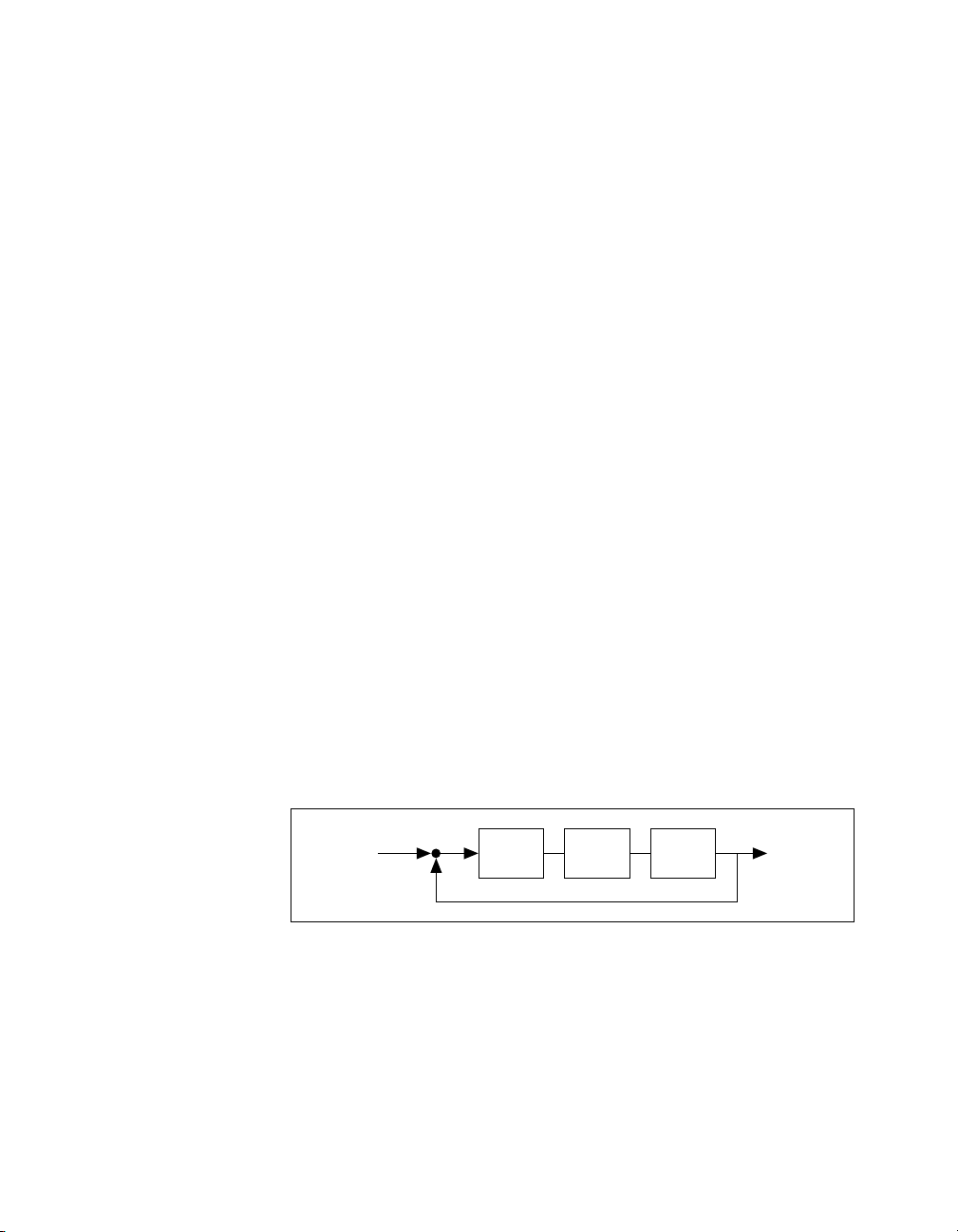
Try to stabilize the system using feedback compensation. You have two major performance goals to achieve through your controller design: first, the system must be closed-loop stable, and second, you want the system output to track a unit step input. To begin, put two compensators in the feedforward path of the closed-loop system. Figure 1-1 is a closed-loop block diagram of helicopter system H(s) with compensators K

(s) and K2(s)

in the feedforward path.

U(s) Y(s)

–

Figure 1-1. Block Diagram of Helicopter System H(s) with Compensators K1(s) and

Xmath Control Design Module 1-6 ni.com

G(s) K1(s) K2(s)

(s) in the Feedforward Path

Chapter 1 Introduction

One approach to stabilizing this system is to try to cancel the pole at –0.656513 by adding a compensator, K

Note It is important to understand that this is primarily an academic exercise. Accurate

(s), with a zero at –0.656513.

pole-zero cancellations are impracticable in the real world, and the mode corresponding to that pole still exists internally.

This compensator must have a pole for realizability, so you add one at –10, which is far enough away that its effect on dynamic response will be small compared to that of the system’s other modes. In addition, you need to add a zero to the left of the positive (and unstable) poles to pull the closed-loop system roots into the left half plane. Choose s = 0 for the zero location and, again, select a corresponding pole at –10. Call this second compensator

(s). To create these two compensators:

K1s=polynomial(ol_poles(3),"s")/...

polynomial(-10,"s");

K2s=polynomial(0,"s")/polynomial(-10,"s");

You then can cascade them in series with the original system Gs (or ssys) and examine the locus of closed-loop roots for varying total compensator gain K

. The poles out at –10 have a smaller effect on the system dynamics

than do the poles closer to the origin, so you can use the optional

rlocus( ) keywords to zoom in on the part of the locus nearer the origin.

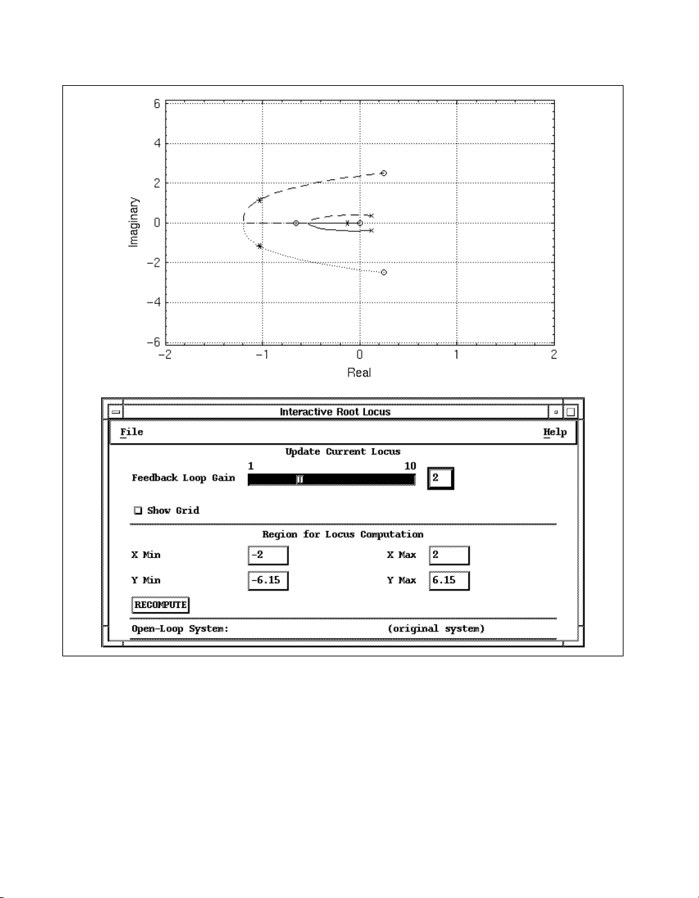
rlocus(K2s*K1s*Gs, {xmin = -2, xmax = 2})

The single input syntax activates interactive mode. A user interface lets you change the gain through the Feedback Loop Gain slider and button. The graphics window shows the closed-loop locus as a solid line, with the open-loop poles shown as large Increase the gain by moving the slider; notice the asterisks (

xs and the open-loop zeros shown as Os.

*) denoting

closed-loop pole location moving along the locus. The system is maximally stable with total compensator gain K figure, small

xs denote the pole location for K

= 2 as shown in Figure 1-2. In this

= 2, and the root locus gain

window shows settings.

Chapter 1 Introduction

Figure 1-2. Locus of all Open-Loop and Closed-Loop Roots of Gs

If you cannot move the slider so that the gain is exactly 2, click the box to the right of the slider and enter

2. To close the interactive root locus dialog

box, select File»Exit.

Xmath Control Design Module 1-8 ni.com

Chapter 1 Introduction

Close the loop using the single-input syntax of feedback( ), which implements direct unity-gain negative feedback, and obtain the system’s step response using

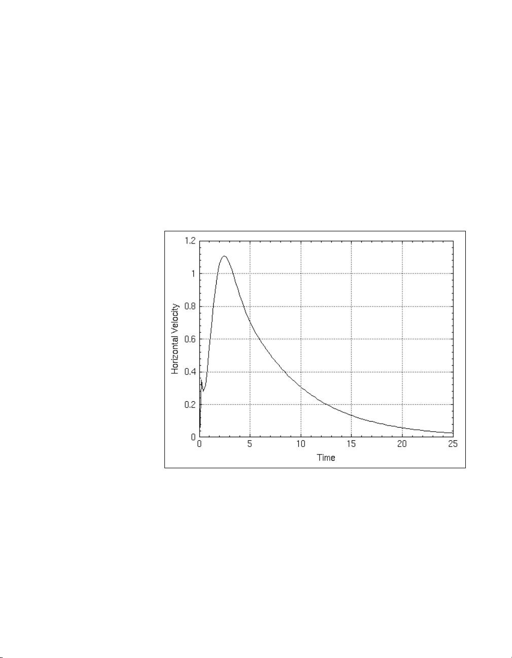
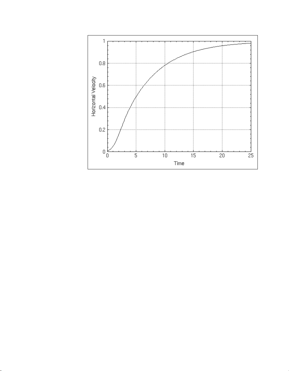
Kc = 2; cl_syscomp1 = feedback(Kc*K1s*K2s*Gs); v = step(cl_syscomp1, 0:.2:25); plot(v,{xlab="Time", ylab="Horizontal Velocity"})

step( ):

The resulting plot is shown in Figure 1-3. This result is not desirable. You want the output (the helicopter velocity) to track the step input provided as the rotor tilt angle, not zero out its effects over time (which would be an appropriate response if the input corresponded to a disturbance). This results from the compensator zero at s = 0 in the forward path of the feedback loop.

Figure 1-3. Helicopter Velocity Response to a Step Input at the Rotor

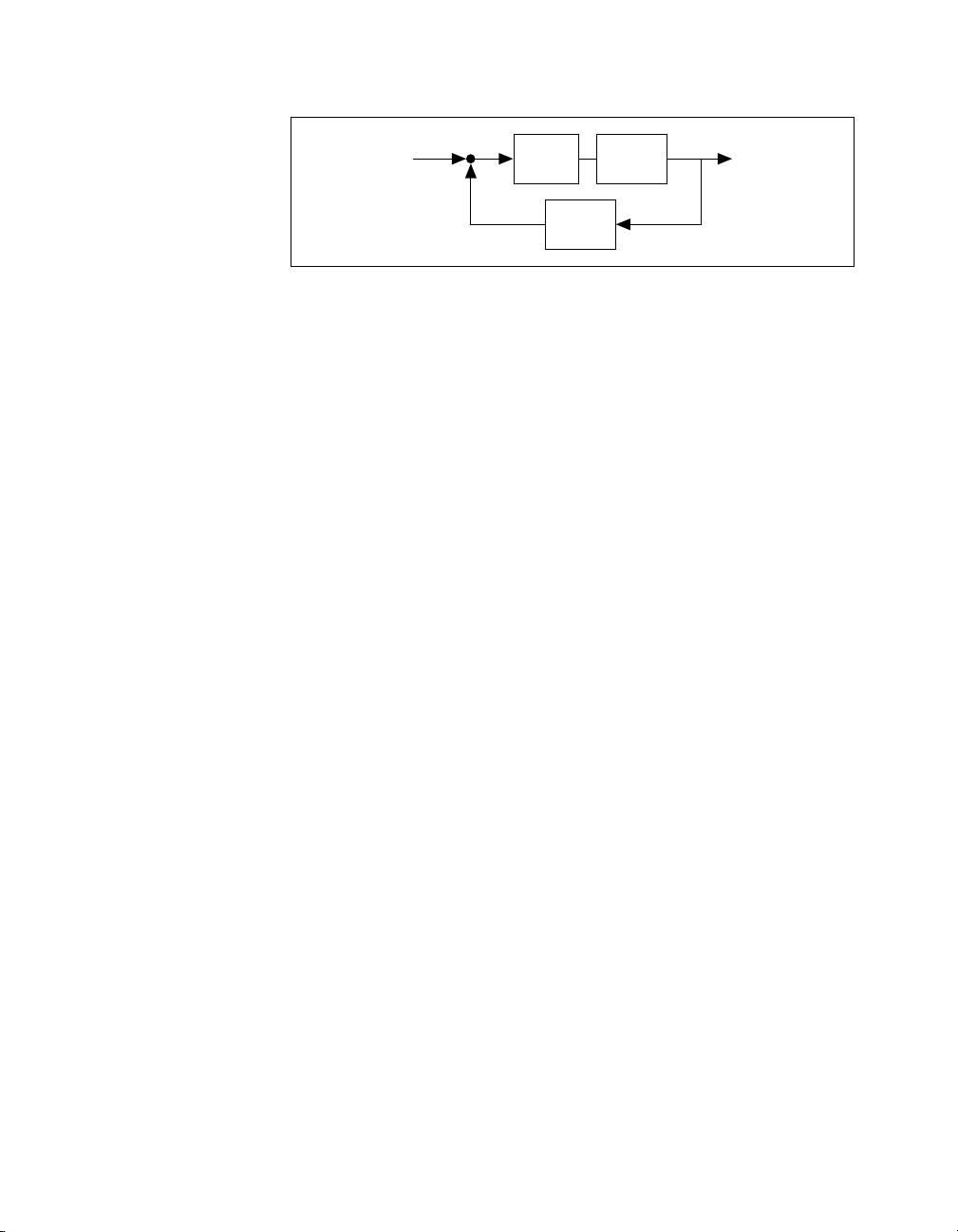
Instead, you now place K1(s) in the forward path and K2(s) in the feedback path, so that the closed-loop system now has the configuration shown in Figure 1-4.

Chapter 1 Introduction

U(s) Y(s)

–

Figure 1-4. Block Diagram of the Closed-Loop Controller

G(s)

Kc1K1(s)

Kc2K2(s)

This is a block diagram of the closed-loop controller with compensator

(s) in the feedforward path and Kc2K2(s) in the feedback path.

c1K1

This time, instead of having all your gain K

in the forward path of the

closed-loop system, the system gain is split between the two compensators. The gains K closed-loop transfer function T

and Kc2 are defined such that Kc=2=Kc1Kc2 and the

(s) is unity at s =0(DC).

The closed-loop transfer function is represented by:

s()Gs()

Tcls()

-------------------------------------------------------------------=

1 K

c1K1

c1Kc2K1

s()K2s()Gs()+

You can find the values of the individual transfer functions at s =0 using

freq( ), and then substitute to solve the previous equation:

a = makematrix(freq(K1s*Gs,0)); b = makematrix(freq(K1s*K2s*Gs,0));

Solving:

Kc1 = (1+2*b)/a

Kc1 (a scalar) = 0.0241778

Kc2 = 2/Kc1

Kc2 (a scalar) = 82.7206

You now call feedback( ) again, this time using its second input argument to indicate that the outputs of the first input system (forward path) are fed back as the inputs to the second system (feedback path) in a negative-feedback loop.

cl_syscomp2 = feedback(Kc1*K1s*Gs, Kc2*K2s);

Xmath Control Design Module 1-10 ni.com

Chapter 1 Introduction

Because cl_syscomp2 contains an internal pole-zero cancellation, you can rewrite it in minimal form and then check the closed-loop pole and zero locations:

cl_syscomp2m = minimal(cl_syscomp2);

The system has 1 uncontrollable state

cl_poles = poles(cl_syscomp2m)

cl_poles (a column vector) =

-0.166518

-1.0325 + 1.16109 j

-1.0325 - 1.16109 j

-37.132

cl_zeros = zeros(cl_syscomp2m)

cl_zeros (a column vector) =

0.25 - 2.4975 j

0.25 + 2.4975 j

-10

Now, examine the step response as shown in Figure 1-5.

vcomp = step(cl_syscomp2m, 0:.1:25); plot (vcomp, {xlab = "Time",

ylab = "Horizontal Velocity"})

Chapter 1 Introduction

Figure 1-5. Helicopter Velocity Tracking Step Input at the Rotor

You also can look at the gain and phase margins of the system.

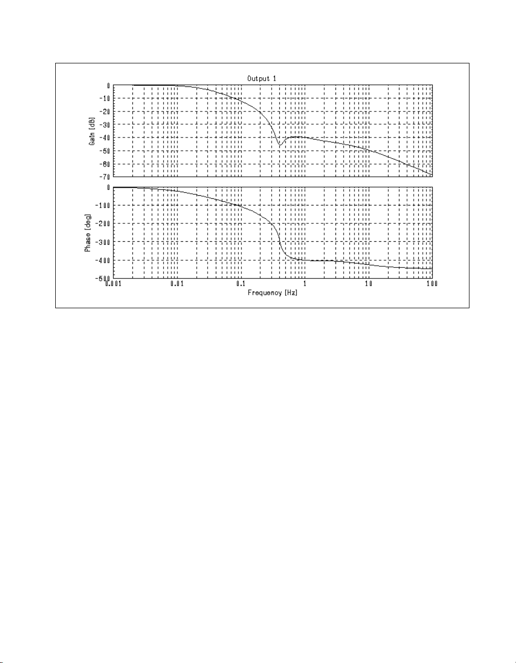
H = bode(cl_syscomp2m, {npts = 200, !wrap}); [gm,pm] = margin(H)

There are no 0 dB gain crossings. gm (a pdm) =

domain |

---------+----------

0.250101 | 26.1694

---------+----------

pm is null

The bode plot of the closed-loop system is shown in Figure 1-6.

Xmath Control Design Module 1-12 ni.com

Chapter 1 Introduction

Figure 1-6. Closed-Loop System Bode Plot

The domain of the gain and phase margin PDMs indicates the frequency (in hertz) at which the margin occurs. So the gain can be increased by about

26.1 dB before the system becomes unstable.

Helicopter Hover Problem: State Feedback and Observer Design

The approach taken in the Helicopter Hover Problem: An Ad Hoc

Approach section, although producing a desirable response, often cannot

be used in practice because uncertainty in modeling generally precludes exact knowledge of the location of the pole one plans to cancel.

Another approach is to feed the information obtained from the states back to the inputs through gains calculated to relocate the closed-loop poles. Refer to the Controllability section of Chapter 6, State-Space Design, for more information. For this approach, you first need to verify that your system is controllable and observable. When you have confirmed that it is—that there are no hidden modes—you can design a full-state feedback control law that will place the system eigenvalues at values that will yield a stable system. Because the system is observable, you then can design an estimator to yield estimates for the missing states. Again, you will require that your system track a step input.

Chapter 1 Introduction

You can verify that your system is controllable, then define the closed-loop poles you want and use

poleplace( ) to find the feedback gains required

given the system A and B matrices.

[,,nuc] = controllable(Gs)

nuc (a scalar) = 0

Because the number of uncontrollable states is zero, Gs is controllable. This means that you can use feedback through appropriately-sized gains to position the system’s closed-loop poles anywhere you want. If you choose the three poles to be moved to –1 ±j and –2, you get the following set of gains:

clp = [-1+jay, -2]; Kfsb = poleplace(A,B,clp)

Kfsb (a row vector) = 0.470648 1.00004 0.062747

Note poleplace( )

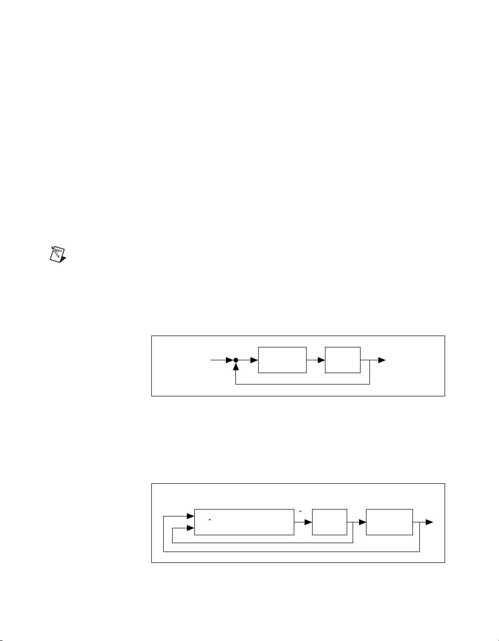
If you assume that the outputs of the system are just the values of all the states, you can draw the open-loop system block diagram as shown in Figure 1-7. In this figure, the feedback path is shown in dotted lines and the open-loop system in solid lines.

Because you do not have access to all three states—only one, the horizontal velocity, is returned as an output—you need to estimate the other states, thus implementing an observer-based controller. The block diagram for the observer and controller together is shown in Figure 1-8.

does not require you to list both poles in a conjugate pair.

ru x

–

Figure 1-7. Full-State Feedback Regulator

Estimator Control Plant

x = (A

– LC)

⋅

x = Ax + Bu

x + Bu

fsb

⋅

fsb

x = Ax + Bu y = Cx + Du

Figure 1-8. Complete Controller and Estimator

Xmath Control Design Module 1-14 ni.com

Chapter 1 Introduction

Specify the observer poles at [–3 + 3j, –4] and call poleplace( ) again:

op = [-3+3*jay, -4];

L = poleplace(A',C',op)

L (a row vector) = 5.46645 4.67623 9.58

You connect the controller to the observer using lqgcomp( ). L needs to be a column vector, so you transpose it.

sys_obc = lqgcomp(ssys, Kfsb, L');

You can use names( ) to modify the names of the state estimates to be more descriptive. To distinguish the estimated states from the “true” states, you can use the

+ operator to append the string est to the estimated state

names, as shown in this example.

[,,osNames] = names(sys_obc); estNames = osNames + [" (est)"," (est)"," (est)"]; estNames'?

ans (a column vector of strings) = Pitch Rate (est) Pitch Angle (est) Horizontal v (est)

You can append these modified names to sys_obc:

sys_obc = system(sys_obc,{stateNames=estNames});

Then you close the loop and verify that the closed-loop poles are all in the left-half plane.

sys_cl = feedback(ssys, sys_obc);

poles(sys_cl)

ans (a column vector) =

-1 + 1 j

-1 - 1 j

-2

-4

-3 + 3 j

-3 - 3 j

Chapter 1 Introduction

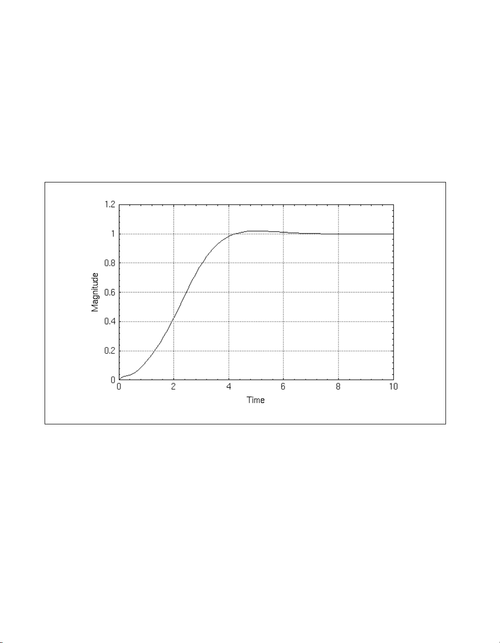
You can choose to scale the system output here for zero steady-state error in the step response. This is accomplished in an intuitive manner, dividing the system

sys_cl = sys_cl/51.76; v_obc = step(sys_cl, 0:.1:10);

plot (v_obc, {xlab = "Time", ylab = "Magnitude"})

sys_cl by the desired scaling factor.

In Figure 1-9 the step response shows zero-steady-state error, little overshoot, and a response time of less than seven seconds.

Figure 1-9. Step Response for Observer-Based Design

The system response is quite good, implying that your state estimates were satisfactory. You can do some further simulation, this time returning all the states directly from the original plant, and get a graphical picture of how the estimates track the actual states. First, you need to create the closed-loop system with all states available.

The

abcd( ) function extracts the A, B, C, and D matrices from a system

object. When you call it here, all you are interested in is the closed-loop A matrix, so you do not need to extract the other state-space matrices.

A_cl = abcd(sys_cl);

Xmath Control Design Module 1-16 ni.com

Chapter 1 Introduction

When you create the estimator system sys_est, you use the original A matrix for the state-update equation, but you provide a zero external input (a B matrix of zero). The output matrix is an identity matrix passing back the three real state values and the three estimated state values as output, again with no external input values affecting the output. Here you use the optional

system( ) keyword X0 to set the real state values to

[1,2,3] and the estimated state values to [–1,–2,–3].

By simulating with a general input over two seconds, you can see how long it takes for the state values provided by the estimator to correct the incorrect initial conditions and track the real state values.

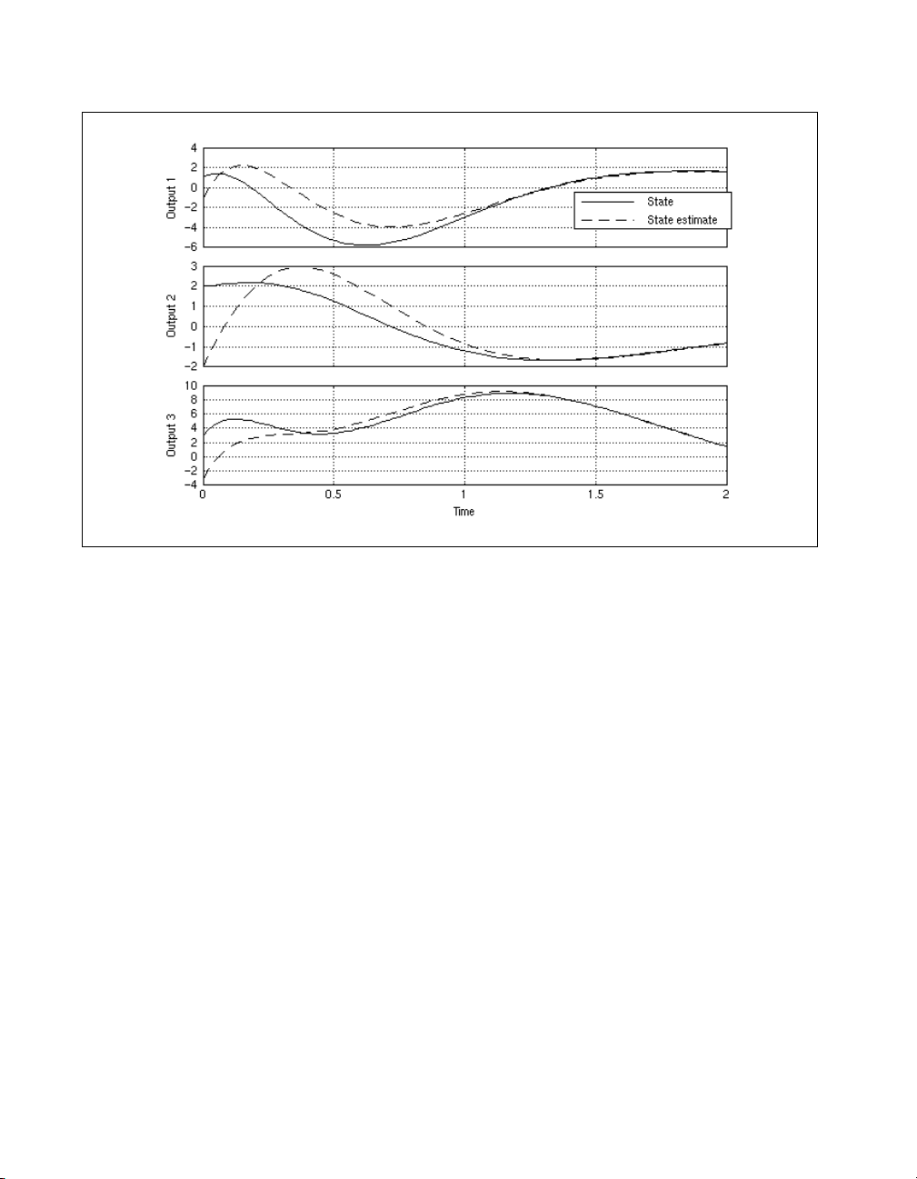
[,,allStates]=names(sys_cl); sys_est = system(A_cl, zeros(6,1), eye(6,6), ...

zeros(6,1),{x0 = [1,2,3,-1,-2,-3], ... stateNames = allStates});

state_resp = sys_est*pdm(ones(100,1), 0:(2/99):2);

Plot the results, referring to Figure 1-10:

plot(state_resp,{strip=2,xlab="Time",

legend=["State","State estimate"]})

Even in the relatively short time span of this simulation, the estimates and the real states quickly converge.

Chapter 1 Introduction

Figure 1-10. Multiple Plots Showing Time Needed for States to be Correctly Tracked

by Estimator, Given Incorrect Initial Values

Helicopter Hover Problem: Discrete Formulation

Discrete-time control systems are most frequently designed in one of two ways: either directly implemented in the discrete domain, or first solved as continuous problems—often deriving directly from differential equations of motion—and then discretized. Here you take the second approach with the problem solved in the Helicopter Hover Problem: State

Feedback and Observer Design section.

A guideline for choosing a sample rate for a system to be discretized is that it be significantly less than the smallest time constant of the continuous system divided by π.

Look at the open-loop pole magnitudes of your original open-loop continuous-time system

max(abs(ol_poles))

ans (a scalar) = 0.656513

Xmath Control Design Module 1-18 ni.com

ssys:

Chapter 1 Introduction

You can use the default exponential discretization method with dt =0.01 and compare frequency responses between the original system and the discretized system:

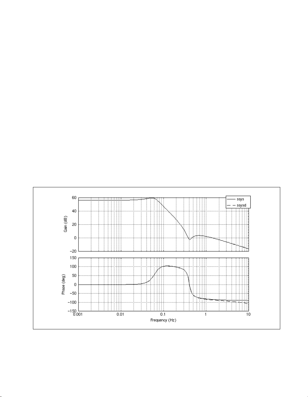
ssysd = discretize(ssys, 0.01); f = freq(ssys,logspace(.001,10,200)); fd = freq(ssysd,logspace(.001,10,200));

In the following statements you compute the gain and phase of both systems and then plot them.

db = 20*log10(abs(f)); ph = (180/pi)*atan2(f); dbd = 20*log10(abs(fd)); phd = (180/pi)*atan2(fd);

plot([db;ph;dbd;phd],{strip=2,xlog,

ylab = ["Gain (dB)";"Phase (deg)"], x_lab = "Frequency (Hz)", legend = ["ssys";"ssysd"]})

In Figure 1-11 you can see the frequency responses match closely, indicating that this discretization method captures the continuous system’s dynamics accurately.

Figure 1-11. Frequency Response of ssys and Its Discrete Equivalent ssysd

Chapter 1 Introduction

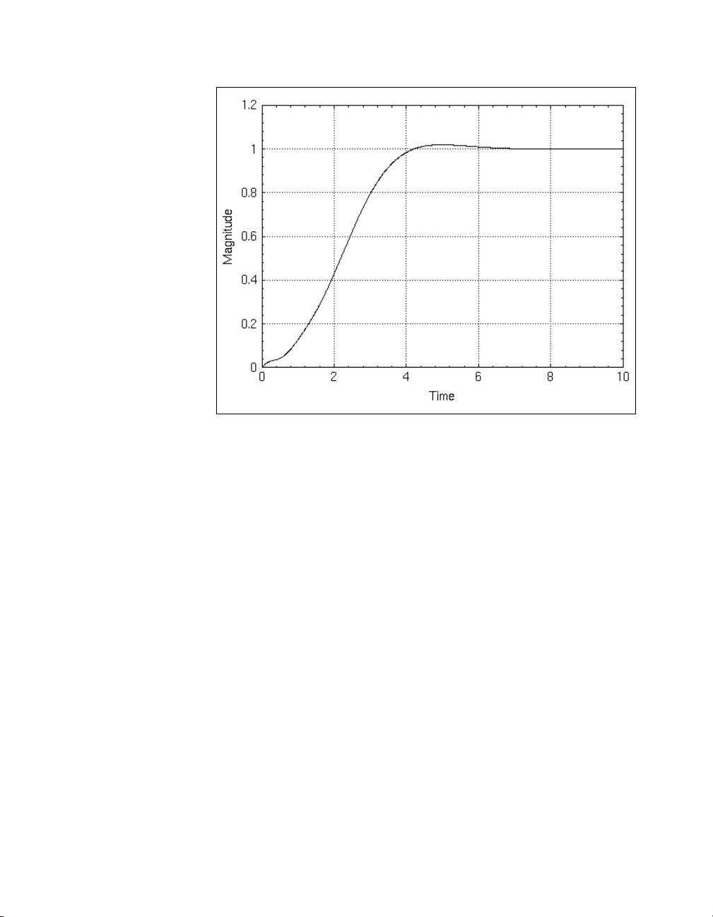
Figure 1-12. Step Response of a Discrete System Using Discretized

Observer-Based Controller

As you discretize the compensator, form the closed-loop, scaled system, and simulate its response to a step input, you must ensure that the sampling interval is the same (

sys_obcd = discretize(sys_obc, 0.01);

sys_cld = feedback(ssysd,sys_obcd)/51.76; v_cld = step(sys_cld, 0:0.01:10); plot (v_cld, {xlab = "Time", ylab = "Magnitude"})

dt = 0.01).

The resulting response is shown in Figure 1-12.

Inverted Wedge-Balancing Problem: LQG Control

[HW91] discusses an approach to balancing an inverted wedge by controlling the location of a sliding mass along the inside of the wedge. This example illustrates use of optimal control with a multi-input, multi-output (MIMO) system. This approach is based on minimizing a quadratic performance index with weight values based on the natural constraints of the system.

Xmath Control Design Module 1-20 ni.com

Chapter 1 Introduction

The linearized state-space equations, including the actuator and sensor dynamics, are as follows:

··

0010

0001

15.54 10.93– 00

5.31– 0 0 16.24–

u+=

1.96

57.29000

0 29.9 0 0

θ is the angle (in radians) the wedge makes with the vertical axis, x is the position of the sliding mass, and u is the control input voltage. The outputs are scaled to give the measured angle in degrees and the measured position in meters.

A = [0,0,1,0;0,0,0,1;

15.54,-10.93,0,0;

-5.31,0,0,-16.24]; B = [0,0,0,1.96]'; C = [57.29,0,0,0;0,29.9,0,0]; D = [0;0];

states = ["Angle", "Mass Position", "Angular Velocity","Mass Velocity"]; wsys = system(A,B,C,D,

{inputNames= "Voltage", stateNames = states, outputNames=["Measured Angle","Measured Position"]});

You need to ensure that you have no uncontrollable or unobservable modes of the system:

[,,nuco] = minimal(wsys)

nuco (a scalar) = 0

Because there are no uncontrollable or unobservable states, you can proceed with the design of a regulator and estimator. The weighting matrix used here in designing the regulator reflects the desire to bring the value of the first state, the angle with the vertical, to zero as quickly as possible.

Chapter 1 Introduction

Because this system is open-loop unstable and has fairly fast poles in both halves of the s-plane, you want to make sure it can bring the effect of an external disturbance (such as a sharp push to the cart) to zero as quickly as possible.

[Kr,EVr,Pr] = regulator(wsys,diag([1e8,1,1,1]),1);

You then can verify that the regulator gain Kr can be used with full-state feedback to control this system by using an identity matrix for C to feed back the states:

[no, ni, ns] = size(wsys); augwsys = system(A,B,eye(ns, ns),[]);

creating the compensator (which is a system object, though it has no states and thus has

comp = system([],[],[],Kr);

NULL A, B, and C matrices) with the gains Kr:

and feeding back the states:

wsysreg = feedback(augwsys, comp);

You then can observe the system response to a sustained disturbance by simulating a five-second step response:

stepreg = step(wsysreg, 0:0.01:5); plot (stepreg, {legend=states,

xlab="Time",ylab="Magnitude", title="System Step Response with "+...

"Full State Availability",!grid})

The resulting plot is shown in Figure 1-13.

Xmath Control Design Module 1-22 ni.com

Chapter 1 Introduction

Figure 1-13. Response of Full-State Feedback Controller to a Unit Step Disturbance

Having established your regulator design, you build the estimator and simulate performance of the closed-loop system feeding back state estimates. You select the weights for the estimator based on the assumption that the state noise intensities corresponding to the wedge angle are smaller than those corresponding to the wedge position. The output weight matrix reflects your higher priority on the wedge angle than position.

The following steps generate the plot shown in Figure 1-14:

[Ke,EVe,Pe] = estimator(wsys,

diag([1e-3,1,1e-3,10]), diag([14,0.01])); wcomp = lqgcomp(wsys,Kr,Ke); wlqg = feedback(wsys,wcomp); resp = step(wlqg,0:0.01:3); plot (resp, {legend = names(wlqg),

xlab = "Time",ylab = "Magnitude",

title = "Observer-Controller System "+...

"Step Response",!grid})

Chapter 1 Introduction

Figure 1-14. Response of Observer-Based Controller to a Unit Step Disturbance

Xmath Control Design Module 1-24 ni.com

Linear System Representation

Xmath provides a structure for system representation called a system object. This object includes system parameters in a data structure designed

to reflect the way these systems are analyzed mathematically. Operations on these systems are likewise defined using operators that mirror as closely as possible the notation control engineers use. This chapter outlines the types of linear systems the system object represents and then discusses the implementation of a system within Xmath. The functions used to create a system object and to extract data from this object are an intrinsic part of the object and are also described. Finally, this chapter discusses the functions

check( ), discretize( ), and makecontinuous( ), which use

information stored in the system object to convert systems from one representation to another.

Linear Systems Represented in Xmath

Xmath handles finite-dimensional, linear, and time-invariant linear systems in both discrete and continuous time. These systems take one of the forms shown in Table 2-1.

Table 2-1. Summary of Linear Systems

System Type Continuous Time Discrete Time

State-spec

Transfer function

The transfer function representation can be used to describe single-input, single output (SISO) systems only; there are no restrictions on the number of input and outputs that can be specified for a state-space system. All of these systems can be created using the Xmath

x·Ax Bu+=

yCxDu+=

Hs() CsI A–()

1–

BD+= Hz() CzI A–()1–BD+=

k 1+

AxkBu

CxkDu

system( ) function.

Chapter 2 Linear System Representation

Transfer Function System Models

One way of representing continuous-time finite-dimensional linear time-invariant systems is with the transfer function:

Hs()

num s()

------------------=

den s()

with num(s) and den(s) being polynomials in s. They can be specified either by their roots or their coefficients. Transfer functions are defined using the Laplace transform operators for continuous time and the forward shift operator z for discrete time. Both forms of transfer functions are written with positive coefficients, each higher order terms having successively larger coefficients.

Discrete systems are defined analogously, using the z variable instead of s. Xmath does not automatically perform cancellations of polynomial roots appearing in both the numerator and the denominator of a transfer function. If you want to cancel common roots in a transfer function, use the function

cancel( ). For state-space systems, refer to the minimal( ) function.

For more information, refer to the Minimal Realizations section of Chapter 6, State-Space Design.

To illustrate how you arrive at a particular transfer function, if you have a system differential equation that takes the form:

y··6y·8y++ 2u·u–=

(2-1)

Laplace-transforming equation (assuming zero initial conditions) yields:

Ys() 6sY s() 8 Ys()++ 2sU s() Us()–=

(2-2)

Collecting terms, you can find the transfer function from U(s) to Y(s), H(s):

Ys()

----------- Hs() Us()

2s 1–

--------------------------==

(2-3)

6s 8++

The roots of the numerator polynomial are the zeros of the transfer function, and the roots of the denominator are its poles. In some circumstances, you might want to construct a transfer function based on where you know the pole and zero locations to be. For example, you can

Xmath Control Design Module 2-2 ni.com

Chapter 2 Linear System Representation

form the same transfer function as that derived in the preceding transfer function equation using known pole, zero, and gain values:

The systems represented in Equations 2-3 and 2-4 can be represented using Xmath’s system objects, as shown in Example 2-1.

The Xmath transfer function system object currently can be used to represent single-input, single-output systems only. State-space form can be used to describe systems with multiple inputs or outputs. For more information, refer to the State-Space System Models section.

Example 2-1 Creating Transfer Functions

The polynomials in the numerator and denominator of the transfer function in Equation 2-3 are both in coefficients form, (described using just coefficients, not roots). them to the

num3 = makepoly([2,-1],"s"); den3 = makepoly([1,6,8],"s"); H3 = system(num3,den3)

system( ) function:

This displays as:

H3 (a transfer function) =

2s - 1

----------

+ 6s + 8 initial integrator outputs 0 0 Input Names

----------Input 1 Output Names

-----------Output 1 System is continuous

Hs()

makepoly( ) creates two polynomials and passes

2 s 0.5–()

---------------------------------=

s 2+()s 4+()

(2-4)

The three statements used to create the transfer function could be more compactly combined as one. The use of s as the variable in which to express the transfer function is optional. Any variable, including the default x, can

Chapter 2 Linear System Representation

be used so long as a consistent choice of variable is used for both numerator and denominator polynomials.

The transfer function in pole-zero-gain form from the preceding equation can be similarly implemented using the specify the numerator and denominator by their roots.

Note The / operator also can be used to create systems in transfer function form, as an

alternative to using

system( ).

H4 = 2*polynomial(0.5,"s")/polynomial([-2,-4],"s")

which displays as:

H4 (a transfer function) =

2(s - 0.5)

--------------

(s + 2)(s + 4)

initial integrator outputs

Input Names

-----------

Input 1

Output Names

------------

Output 1

System is continuous

polynomial( ) function to

In both of these cases you have created a continuous system. Systems created in Xmath contain sample rate information as well as the numbers representing system dynamics. However, unless a sample rate is explicitly given as a keyword to

system( ), it defaults to zero and the system is

continuous. For an illustration of how to create a discrete system, refer to Example 2-2. The full discussion of the

system( ) function in the

system( ) section contains a listing of all the keywords associated with

system( ).

Xmath Control Design Module 2-4 ni.com

State-Space System Models

State-space models comprise the second category of linear system representations in Xmath. In state-space form, first-order differential (continuous-time) and difference (discrete-time) equations are represented as a set of state and output updates. The states are represented by a vector x; u and y are vectors with as many elements as there are inputs and outputs, respectively. This system model is useful for representing multi-input, multi-output (MIMO) systems.

continuous time:

discrete time:

Chapter 2 Linear System Representation

x·Ax Bu+=

yCxDu+=

A straightforward mathematical transformation from the state-space form to the transfer function form is as follows:

Hq() CqI A–()

All of the forms represented in these equations can be represented using Xmath’s system objects, as shown in Example 2-2.

Example 2-2 Creating a Discrete State-Space System

Suppose you have a system which you describe in state-space form as:

and you know that the sample period of the system is 0.5 seconds between samples—that is, the states and outputs are updated at every discrete interval k, consisting in this case of 0.5 seconds.

k 1+

AxkBu

CxkDu

0.75– 0

1–

BD+=

Chapter 2 Linear System Representation

Again, you create the system using the system( ) function. This time you use the optional

A = [0,1;-0.75,0]; B = [1,0]'; C = [0,1]; D = 0; sys4 = system(A,B,C,D, {dt = 0.5})

sys4 (a state space system) =

System is discrete, sampling at 0.5 seconds.

dt keyword to indicate that this system is discrete.

0 1

-0.75 0

0 1

Although five lines of MathScript were used to be as explicit as possible in creating this system, the call to

Note When you create a system object, its inputs (A, B, C, D) are no longer needed.

system( ) can encompass all of them.

Basic System Building Functions

The functions discussed in the following sections are available with the general Xmath package. However, Control Design Module users will find these functions an intrinsic part of their work, warranting this discussion. The Xmath Help provides additional details about these functions and examples of their use.

system( )

Sysd=system(A,B,C,D,{dt,inputNames,

outputNames,stateNames,X0}) Sys = system(num,den,{dt,inputNames,outputNames}) Sys = system(Sys,{keywords})

Xmath Control Design Module 2-6 ni.com

Chapter 2 Linear System Representation

The system( ) function can create both the transfer-function and state-space forms of the system object. It requires four compatibly-sized matrices to create a state-space system, or a pair of polynomials to create a transfer function.

You can use optional keywords to store additional information about your system. Assigning discrete, with a sampling period equal to that value. If

dt to a positive scalar value indicates that the system is

dt is not specified,

the system is continuous, with a sampling period defaulting to zero. Because information indicating whether the system is continuous or discrete is encapsulated within the system object itself, Xmath does not have separate functions for discrete- and continuous-time system analysis. Systems can be recognized by Xmath’s functions as discrete or continuous using the

check( ) function and handled accordingly. For more

information, refer to the Using check( ) with System Objects section. The capability to assign a discrete sample rate does not actually discretize a continuous-time system, however. For information on discretizing a system, refer to the Discretizing a System section.

A shortcut for creating state-space systems with an all-zero D matrix is to use a null-matrix specifier

([]) for the D matrix instead of entering an

appropriately sized zero matrix. This will automatically set the D matrix to be a zero matrix with row size equal to the row size of C, and column size equal to the column size of B.

In addition, descriptive names for the inputs and outputs of a system can be specified as vectors of string names and assigned to the

outputNames, and stateNames keywords. stateNames is valid only

when used in conjunction with a state-space system, as is the keyword

inputNames,

X0,

which can be used to set a vector of initial values for the states.

When you have created a system, you can modify it by changing the values of any of the keywords discussed in this section by calling

system( ) with

the appropriate keyword setting.

Examples 2-1 and 2-2 illustrate how transfer function and state-space system, respectively.

system( ) can be called to create a

system( ) also can

be used to change the attributes of an existing system.

Note In Example 2-3, the [] notation indicates that the D matrix should be an

appropriately sized (in this case, scalar) zero matrix.

Chapter 2 Linear System Representation

Example 2-3 Using system( ) to Change the Attributes of an Existing System

sys4=system([0,1;-0.75,0],[1,0]',[0,1],[],

{dt=0.5});

sys4 = system(sys4, {inputNames = "Current",

outputNames = "Velocity",

stateNames = ["Torque","Angle"]})

sys4 (a state space system) =

0 1

-0.75 0

0 1

0 0

State Names

----------Torque Angle

Input Names

----------Current

Output Names

-----------Velocity

System is discrete, sampling at 0.5 seconds.

abcd( )

[A,B,C,D,X0] = abcd(Sys)

The abcd( ) function extracts the component A, B, C, and D matrices described in equations from a state-space system object as shown in the

State-Space System Models section. In addition, it returns the initial

conditions on the states if a fifth output argument is requested.

abcd( ) can be called on systems in either state-space or transfer function

form. If the system is a transfer function, the conversion to state-space is

Xmath Control Design Module 2-8 ni.com

done internally to return A, B, C, and D, though the format of the variable

Sys itself remains unchanged. The transfer function must be proper.

Using the systems defined in Examples 2-1 and 2-2, Example 2-4 illustrates the use of

Example 2-4 Using abcd( ) to Extract the State-Space Matrices

H3=makepoly([2,-1],"s")/makepoly([1,6,8],"s");

sys4=system([0,1;-0.75,0],[1,0]',[0,1],0,

{dt=0.5});

abcd( ).

You can extract the state-space matrices from each.

Note For the transfer function H3, an internal conversion is performed.

[A3,B3,C3,D3] = abcd(H3)?

A3 (a square matrix) =

-2 1.58114 0 -4

B3 (a column vector) =

0 2

C3 (a row vector) = -1.58114 1 D3 (a scalar) = 0

[A4,B4,C4,D4,X0] = abcd(sys4)

A4 (a square matrix) =

0 1

-0.75 0

B4 (a column vector) =

1 0

C4 (a row vector) = 0 1 D4 (a scalar) = 0 X0 (a column vector) =

0 0

Chapter 2 Linear System Representation

numden( )

[num,den] = numden(Sys)

The numden( ) function returns the numerator and denominator polynomials comprising a single-input, single-output system in transfer function form. If the system is in state-space form, an internal conversion is performed to find the transfer function equivalent, but the format of the system variable itself remains unchanged. State-space systems used in conjunction with

As noted in the Transfer Function System Models section, common roots in the numerator and denominator polynomials are not canceled.

Example 2-5 uses the state-space system from Example 2-2 to illustrate the use of

numden( ).

Example 2-5 Using numden( ) to Extract the Transfer Function Polynomials

sys4=system([0,1;-0.75,0],[1,0]',[0,1],0,

{dt=0.5});

[num,den] = numden(sys4)?

num (a polynomial) =

-0.75

den (a polynomial) =

+ 0.75)

numden( ) must be single-input, single-output.

Because num and den are polynomial objects and not a complete system, the discrete sampling time is not explicitly saved. You can use with the

convert keyword to map the two internal representations to each

check( )

other, as described in the Using check( ) with System Objects section. However, notice that z was used as the polynomial variable, indicating that these numerator and denominator polynomials were obtained from a discrete-time system. Had the system been continuous, s would have been used instead of z.

period( )

dt = period(Sys)

The period( ) function extracts the sample period (in seconds) of a system. If the system is continuous,

In Example 2-5, you found the numerator and denominator polynomials corresponding to the discrete state-space system. Example 2-6 combines

Xmath Control Design Module 2-10 ni.com

period( ) will return zero.

these polynomials into a transfer-function and uses period( ) to set the sampling interval to match that of

Example 2-6 Using period( ) to Extract the Sampling Period

[num,den]=numden(sys4);

H4 = system(num,den,{dt = period(sys4)})

H4 (a transfer function) =

-0.75

-----------

+ 0.75)

System is discrete, sampling at 0.5 seconds.

Chapter 2 Linear System Representation

sys4.

check( )

provides a more concise means of converting between

state-space and transfer function form, as described in the Using check( )

with System Objects section, but this example illustrates how the output of

one function can be specified directly as keyword input to another.

names( )

[outputNames,inputNames,stateNames] = names(Sys)

The names( ) function extracts matrices of strings representing the input, output, and (if the system is in state space form) state names of a system.

names( ) also can be used to extract information from the PDM and

polynomial objects. More information on these functions can be found in the MATRIXx Help.

When you create a system without specifying any names, a default set of names are assigned to it. Unlike user-specified names, these default names are not displayed in the Xmath Commands subset of the names you select to store with the system still can be extracted using

names( ) as shown in Example 2-7.

Example 2-7 Using names( ) to Extract the Variable Names Associated with a System

H3 = system(makepoly([2,-1],"s"),

makepoly([1,6,8],"s"));

[outputNames, inputNames] = names(H3)

outputNames (a string) = Output 1 inputNames (a string) = Input 1

sys5=system([0,1;-0.75,0],[1,0]',[0,1],0,{dt=0.5,

inputNames = "Current",

window. However, all, or any

Chapter 2 Linear System Representation

outputNames = "Velocity", stateNames = ["Torque","Angle"]});

[,,stateNames] = names(sys5)?

statenames (a row vector of strings)=Torque Angle

Size and Indexing of Dynamic Systems

The size of a system object is defined by how many outputs, inputs, and (in the case of a state-space system) states it has. You can use the function to find these dimensions.

You can index into a dynamic system to create a new dynamic system which has a subset of the original inputs and outputs:

Sys = Sys1(i,j) is defined to be a system such that y = y1(i) and u = u1(j). i and j can both be vectors as well, in which case multiple inputs and

outputs will be extracted.

The previous definition of indexing was designed with the traditional definition of a transfer function in mind.

size( )

yq() Sys q() uq()×=

Using check( ) with System Objects

Several common attributes of systems can be easily determined using Xmath’s ability to distinguish between object types and characteristics. You can use the Example 2-8, to determine whether a system is in transfer function or state-space form, discrete, continuous, or stable. In addition, you can use

check( ) with the convert keyword to change a system’s representation

between SISO state-space and transfer-function forms.

Example 2-8 Using check( ) with a System

a = [1.875,0;0,-0.26]; b = [1;0]; c = [0.5,1]; d = 0; sys = system(a,b,c,d, {dt = 0.001});

Because this system is discrete and has a pole where magnitude exceeds 1, it is not stable.

check( ) function with systems, as shown in

Xmath Control Design Module 2-12 ni.com

check(sys, {stable})

ans (a scalar) = 0

check(sys, {discrete, ss})

ans (a scalar) = 1

[, tfsys] = check(sys, {tf, convert})

tfsys (a transfer function) =

(z + 0.26)

--------------------(z + 0.26)(z - 1.875)

initial delay outputs 0 0

System is discrete, sampling at 0.001 seconds.

Discretizing a System

Many systems where behavior derives from physical equations of motion can be modeled most naturally as continuous processes, using differential equations. Therefore, you often choose to discretize these models for use with a digital controller. A number of mathematical methods have been developed to approximate the behavior of a continuous system in a discrete-time representation with an appropriately fast sampling rate. Xmath provides two functions,

makecontinuous( ), which encompass a range of these techniques. discretize( ) converts a system from its representation as a continuous

function in the s-domain to a discrete-time z-domain function.

makecontinuous( ) does the reverse, transforming a discrete system to

its continuous form.

Chapter 2 Linear System Representation

discretize( ) and

discretize( )

SysD = discretize(Sys,{dt,exponential,forward,backward,

tustins,ztransform,polezero,firstorder})

The discretize( ) function has a number of keywords that correspond to the different methods of continuous-to-discrete conversion that are implemented within Xmath. The sampling interval (in seconds) for the discrete system should be set equal to the keyword is specified, a default of 0.5 seconds is used. The default discretization method used is the exponential (step-invariant) transform. The different

dt. If no value for dt

Chapter 2 Linear System Representation

discretization methods used based on the specification of each keyword are discussed in the following sections.

Numerical Integration Methods: forward, backward, tustins

Xmath provides three methods of numerical integration of a differential transfer function: the forward and backward rectangular rules, and Tustin’s rule (also called the bilinear or trapezoidal transform).

To convert the system description from a continuous differential equation to a discrete difference equation, you approximate the value of the derivative in the continuous equation over each find the area of the geometric region having width the derivative. You can do this in a number of ways, as discussed in [FPW90].

For the forward rectangular method, you assume the incremental area term between sampling times k * dt and (k +1)*dt to be a rectangle having width dt and height equal to the integral form of the differential equation at time (k +1)*dt. In essence, you get your amplitude estimate for each rectangle by looking forward, hence the name. The backward rectangular method arises similarly, except that you get the rectangle’s height by looking backward and taking the value of the integral at k * dt. The forward rectangular approach tends to overestimate the incremental area somewhat and the backward approach tends to underestimate it (though with a sufficiently small sampling interval, this may not pose a large problem). The trapezoid rule strikes a balance between these two methods by taking the average of the rectangles defined by the forward and backward methods and using that value as the incremental area in approximating the difference equation.

dt seconds of time, then

dt and height equal to

These approaches can be summarized as substitutions between the continuous-time Laplace-transform operators and the discrete z-transform operator z as shown in Table 2-1.

Table 2-2. Mapping Methods for discretize( )

Method of Approximation Continuous to Discrete

Forward rectangular rule: Keyword:

Xmath Control Design Module 2-14 ni.com

forward

z 1–

-----------

→

Chapter 2 Linear System Representation

Table 2-2. Mapping Methods for discretize( ) (Continued)

Method of Approximation Continuous to Discrete

Backward rectangular rule: Keyword:

Tustin’s rule: Keyword:

backward

tustins

z 1–

-----------

→

zdt

2 z 1–()

---------------------

→

dt z 1+()

Pole-Zero Matching: polezero

The pole-zero matching method of discretizing a continuous system follows from the relation between the continuous s and discrete z frequency domains:

where T is the sampling interval to be used for the discrete system. Continuous-time poles and finite zeros are mapped to the z-plane using this relation. Zeros at infinity are mapped into z = 0, where they do not affect the frequency response.

After the poles and zeros have been mapped, the algorithm tries to make sure the system gains are equivalent at some critical frequency. If the systems have no poles or zeros at DC(s =0,z = 1), the discrete-time gain is selected such that the system gains match at DC. Alternatively, if the systems have no poles or zeros at the Nyquist frequency (s = p *j/T, z = –1), the gains are equalized at that frequency. In the event that neither of these gains can be matched, no gain is chosen.

Z-Transform: ztransform

This method is a direct Z-transform of the continuous-time transfer function, which corresponds to the Z-transform of the impulse response of the system. If of the continuous and discrete systems. The responses may differ slightly due to round off error.

ztransform is used, you will match the impulse responses

Hold Equivalence Methods: exponential and firstorder

The discretization methods for exponential and firstorder both rely on the approximation that the discrete-time response can be represented as a hold on the sampled values of the continuous-time response.

Chapter 2 Linear System Representation

The exponential keyword assumes that the response value between samples is constant and can, therefore, be represented by a zero-order hold polynomial. When response is discretized using th e Z-transform, then the result is divided by the Z-transform of a step z/(z – 1) to produce the desired transfer function.

The

firstorder keyword assumes extrapolation between samples

(connecting sample to sample in a straight line). If specified, the continuous-time ramp response is discretized using the Z-transform and then the result is divided by the Z-transform of a ramp z * dt/(z – 1)2 to produce the desired transfer function.

In each of these cases, the appropriate response (impulse, step, or ramp) will match the continuous response very closely, with the only error being round off error.

While no one method of discretization will always perform best for all systems and all sampling times, it is often a good idea to compare the frequency response resulting from different discretized models to the continuous response. Example 2-9 applies the forward, backward, tustins, exponential, and matched pole-zero discretization methods.

exponential is specified, the continuous-time step

firstorder is

Example 2-9 A Comparison of Several Discretization Methods

H = system(0.5*polynomial([-0.36]),

makepoly([1,2.79,2.74,1.11,0.16]));

Create a logspaced vector for the frequency range of the response:

F = logspace(.001,5,200);

Perform the discretization using the different algorithms:

Hd_f = discretize(H,0.1,{forward}); Hd_b = discretize(H,0.1,{backward}); Hd_t = discretize(H,0.1,{tustins}); Hd_z = discretize(H,0.1,{polezero}); Hd_e = discretize(H,0.1,{exponential});

Now you can calculate the magnitude response as a function of frequency,

gainc = 20*log10(abs(freq(H,F)));

gain_f = 20*log10(abs(freq(Hd_f,F)));

gain_b = 20*log10(abs(freq(Hd_b,F)));

gain_t = 20*log10(abs(freq(Hd_t,F)));

Xmath Control Design Module 2-16 ni.com

Chapter 2 Linear System Representation

gain_z = 20*log10(abs(freq(Hd_z,F)));

gain_e = 20*log10(abs(freq(Hd_e,F)));

and plot it (as shown in Figure 2-1).

plot ([gainc,gain_f,gain_b,gain_t,gain_z,gain_e],

{legend = ["Continuous", "Forward",

"Backward", "Tustins", "Pole Zero", "Exponential"], x_log,

xlab="Frequency (Hz)",ylab="Magnitude (dB)"})

Figure 2-1. Comparison of Different Frequency Response Techniques

Although most of the discretizations used would give acceptable approximations to the continuous-time response, notice that most of them diverge greatly at higher frequencies. You may find it illustrative to run this example with larger and smaller sampling intervals to see how the choice of sampling rate, as well as the choice of method, affects the accuracy of the discretized frequency response.

makecontinuous( )

Sys=makecontinuous(SysD,{exponential, forward,

backward,tustins, ztransform})

Chapter 2 Linear System Representation

Many of the discretization techniques discussed in the Hold Equivalence

Methods: exponential and firstorder section can be easily reversed to

obtain a continuous equivalent to a discrete system. The

makecontinuous( ) function implements these reverse algorithms

based on the keyword you specify as shown in Example 2-10. Although

makecontinuous( ) accepts an input system in any form, it returns the

continuous-time system as a state-space system.

The forward, backward, and Tustin methods for mapping from the s-plane to the z-plane can be easily reversed using the equivalencies shown in Tabl e 2-3.

Method of Approximation Discrete to Continuous

Table 2-3. Mapping Methods for makecontinuous( )

Forward rectangular rule: Keyword:

forward

Backward rectangular rule: Keyword:

backward

Tustin’s rule: Keyword:

tustins

Discrete-to-continuous algorithms using matrix logarithms (to reverse the exponential operations involved in doing the z-transform for the impulse invariant zero-order hold) are available for the (step-invariant) transformation and the methods. A limitation of these methods, however, is that they will not return a meaningful continuous equivalent to a discrete system that has pure delays (1/z terms), because the logarithm of zero is infinite.

Example 2-10 Verifying a Discretization Using makecontinuous( )

Create a system:

H = 0.5*polynomial([-0.36])/...

polynomial([-1,-1,-0.395+0.06305*jay,

-0.395-0.06305*jay]);

Form the discrete equivalent using the forward approximation:

Hd_f = discretize(H,0.1, {forward});

z 1 sdt()+→

---------------------

→

1 sdt()–

1 sdt()+ 2⁄

----------------------------

→

1 sdt()– 2⁄

exponential

ztransform (impulse-invariant)

Xmath Control Design Module 2-18 ni.com

Chapter 2 Linear System Representation

Now convert back to the continuous form:

Hc = makecontinuous(Hd_f, {forward}); [num,den] = numden(Hc)

num (a polynomial) =

(s + 0.36)

den (a polynomial) =

(s + 0.999998)(s + 1)(s + 0.79s + 0.16)

Although makecontinuous( ) restores the continuous-time poles and zeros, it cannot match gains precisely.

Building System Connections

Large system models are frequently built by connecting smaller models together. You can perform different types of linear system interconnections using the Xmath functions discussed in this chapter.

MathScript allows operators ( different behaviors when used with different objects. A number of simple types of connections have been implemented as overloaded operators on systems, while more complex connections are available through specialized functions.

*,+, and so on) to be overloaded—given

Linear System Interconnection Operators

Overloaded operators provide a quick way to perform different types of basic connections between systems. Table 3-1 illustrates these operations

Diagram Description

Sys = Sys1 + Sys2

Sys1

Sys2

on a pair of systems and

, respectively.

Table 3-1. Summary of Interconnection Operators

Sys

and Sys2 with outputs y1 and y2 and inputs u1

Parallel connection where y = y tied together where

u=u1=u

+ y

. The inputs are

Sys = Sys1 – Sys2

Sys1

Sys2

–

Parallel connection where y = y case

, Sys = –Sys

together where

where y=–y1. The inputs are tied

u=u1=u

+ y

. In the unary

Chapter 3 Building System Connections

Table 3-1. Summary of Interconnection Operators (Continued)

Diagram Description

Sys = Sys2 * Sys1

u1 u2y1 y2

Sys1

Sys = Sys1/Sys2

u2 u1y2 y1

inv(Sys2)

Sys = Sys1\Sys2

u2 u1y2 y1

Sys2

Sys = [Sys1;Sys2

Sys1

Sys2

Sys1

inv(Sys1)

Cascade connection of Sys1 and Sys2 where the output of

Sys is y

and the input is u1.

Cascade connection of Sys1 and inverted Sys2 where

Sys = Sys1* inv(Sys2), u=u

, and y = y1.

Cascade connection of inverted Sys1 and Sys2 where

Sys = inv(Sys1) * Sys2, u = u

Parallel connection where y = [y tied together where

u=u1=u.

, and y = y1.

]. The inputs are

1;y2

Sys = [Sys1,Sys2

Parallel connection where y = y

+ y

and

u =[u1;u2].

Sys = Sys1'

Sys1

Sys2

If Sys1 is in state-space form and comprises the matrices (

A1,B1,C1,D

Sys

), Sys comprises (A

is a transfer function, it is converted internally

',C1',B1',D1').

to state-space form.

Xmath Control Design Module 3-2 ni.com

Chapter 3 Building System Connections

Table 3-1. Summary of Interconnection Operators (Continued)

Diagram Description

Sys = adj[Sys1]

p1/p2

Sys = inv(Sys1)

If Sys1 is in state-space form and comprises the matrices (

A1,B1,C1,D

(

–A1',C1',B1',D1'). If Sys

), Sys is the adjoint system and comprises

is a transfer function, it is

converted internally to state-space form.

Alternate method to create a system, where p1 and p2 are the numerator and denominator polynomials, respectively; does not allow the use of keywords.

The inverse (pseudoinverse) of a system can be found using

inv(Sys1). If Sys

inv(Sys1) is the reciprocal of the transfer function.

Sys

is a state-space system (A1,B1,C1,D1), then

Sys = system(A,B,C,D) where A,B,C,D are defined

is a transfer function,

as follows:

D = pinv(D1) A = A1-B1*D*C1 B = B1*D C = -D*C1

Dynamic systems also can be flexibly combined with scalars and compatibly sized matrices using the operators in Table 3-1. A compatibly sized matrix is one having the same dimensions as the dynamic system’s D matrix (row size equal to the number of outputs and column size equal to the number of inputs).

Operations performed with a dynamic system and a matrix M as the operands internally handle M as a pure-gain system implemented as

system([],[],[],M).

The

* operator can be used with a system and a PDM to find the time

response of the system to the general input data stored in the PDM. For a detailed description of time simulation in Xmath, refer to the General

Time-Domain Simulation section of Chapter 4, System Analysis.

Chapter 3 Building System Connections

Linear System Interconnection Functions

afeedback( ), append( ), connect( ), and feedback( ) connect

dynamic systems in state–space or transfer–function form to produce a larger system in state-space form. The following restrictions apply to all of these functions:

• Both systems must have the same sample rate.

• Improper dynamic systems (systems with more zeros than poles) are not allowed.

• If the systems to be connected are in transfer-function form, they must be expressed in the same dependent variable.

In describing the algorithms used in these connection functions, we will often refer to the component matrices of a state-space system

, C1, and D1.

afeedback( )

Sys = afeedback(Sys1,{Sys2})

The afeedback( ) function connects two dynamic systems in a feedback loop, and obtains a single system representation for the complex loop.

Sys is organized as shown in Figure 3-1. Additional external inputs to the

feedback path are included with outputs from the feedforward path. Figure 3-1 illustrates that outputs of the feedback path system are included with forward path outputs refer to Example 3-1.

. For an example of how to use afeedback( ),

Sys

as A1,

Sys

–

Sys

Figure 3-1. afeedback System Configuration

Xmath Control Design Module 3-4 ni.com

• By default, feedback is defined to be negative.

• The number of outputs from the first system must equal the number of inputs to the second system.

• The number of outputs from the second system must equal the number of inputs in the first.

• Both systems must have the same sample rate.

• Improper dynamic systems (systems with more zeros than poles) are not allowed.

• When only one system is specified, it must be square (it must have an equal number of inputs and outputs).

Example 3-1 Using afeedback( ) to Connect Two Systems

Sys1 = system([.5,1;0,2],[1,0]',[0,1],0);

Sys2 = system([1,-.2;1,0],[1,0]',[1,1],0);

saf = afeedback(Sys1,Sys2);

Algorithm

If only one system input (Sys1) is provided to afeedback( ), the second input (

Sys

) defaults to a zero-state system with unity gain. This is

analogous to a state-space system with matrices, and with an identity matrix for D. Notice that you use the Xmath definition of a non-square identity matrix. In this case, the row dimension of D equals the number of inputs to the number of outputs of Sys state-space matrices of convention for

Sys

Chapter 3 Building System Connections

NULL values for the A, B, and C

Sys

, and the column dimension equals

. In the following discussion, you denote the

by A1, B1, C1, and D1, and you follow the same

The two systems are first internally converted to a state-space form, if necessary, and subdivided into the A, B, C, and D state-space matrices. Scaling matrices S1

and S2 are computed for Sys1 and Sys

= I + D1D

S2 = I + D2D

as follows:

Additionally, you define:

= B1/S2 and D1s = D1/S

B2s = B2/S1 and D2s = D2/S

Matrix right-division problems must be well-posed, with the scaling matrices S

and S2 nonsingular. afeedback( ) displays an error message

Chapter 3 Building System Connections

if the condition estimate for either matrix is less than eps. For more information on this condition estimate, refer to the MATRIXx Help for the Xmath function

Using feedback loop, you can express its component matrices A, B, C, and D as combinations of the component matrices you obtained from

Sys

. The full matrices used with two input systems are shown in the next

example. In the case of a constant-gain feedback, A, B, C, and D are computed using only the matrix partitions shown in bold type.

The initial conditions for the systems are appended to each other columnwise.

rcond( ).

Sys to denote the state-space representation for the complete

Sys

2sC1

2sD1B2s

B1sD

–

– B1sC

1B1sD2C1

–

A2B2sD1C

–

and

⁄ D1sC

–

1C1

2sC1S2C2

2D1s

afeedback( ) cannot be used with improper transfer functions—systems

D1D

–

having more zeros than poles—because this algorithm is strictly state-space.

append( )

Sys = append(Sys1,Sys2)

The append( ) function appends two dynamic systems in a form suitable for use with the

Xmath Control Design Module 3-6 ni.com

connect( ) function (refer to the connect( ) section). Sys

Chapter 3 Building System Connections

is created by appending the inputs, outputs, and states of Sys1 and Sys2. A larger number of systems can be appended by appending two at a time.

• Both systems must have the same sample rate.

• Improper dynamic systems—systems with more zeros than poles—are not allowed, because

Sys is represented in state-space form.

The output is a dynamic system in block form as shown in Figure 3-2.

For an example of how to use append( ), refer to Example 3-2.

Example 3-2 Using append( )

s3 = system(makepoly([1,2]), makepoly([1,3,5,0])); s4 = system(makepoly([1]), makepoly([1,4,4])); sap = append(s3,s4);

In the following discussion, the component state-space matrices of Sys1 are denoted by

The algorithm for representations of be improper transfer functions (transfer functions having more zeros than poles). The component A, B, C, and D matrices of extracted using the comprising zero matrix elements span as many rows and columns as necessary.

Sys

Figure 3-2. Output of a Dynamic System

, B1, C1, and D1, and you follow the same convention for Sys2.

append( ) is done strictly using the state-space Sys

and Sys2. For this reason, Sys1 and Sys2 cannot

Sys

and Sys2 are

abcd( ) function. The A, B, C, and D matrices

Sys are obtained as shown in the following example, where the

Chapter 3 Building System Connections

connect( )

= B

0 A

= D

0 C

append( ) performs a check to make sure both Sys

0 B

0 D

and Sys2 have the

same sample rate, and adopts this rate for the appended system. Any initial conditions on the states are also appended columnwise.

Sys = connect(Sys1,{K,M,N})

The connect( ) function performs a general interconnection around a system. This provides two basic capabilities:

• constant gain feedback

• general input–output interconnection

In its simplest form, feedback around a system. The keyword

connect( ) can be used to wrap constant gain

K, used to specify feedback gain,

also can be used to specify which outputs are fed back to the input of the system. By specifying the optional keywords

M and N, you also can specify

input and output gains.

General input–output interconnection is applicable to the block form system provided by Parameters used in the

append( ), as described in the append( ) section.

connect command are illustrated in Figure 3-3.

Notice that feedback is defined with a positive sign.

uyy

Figure 3-3. Parameters Used with the connect Command

Xmath Control Design Module 3-8 ni.com

Sys

Chapter 3 Building System Connections

• By default, feedback is defined to be positive. To enforce negative feedback, specify

connect(Sys,-K).

• A “selection matrix” has a single 1 in each row; the rest of the row contains zeros. This is useful for indicating the subset of system inputs and outputs to be used. In many cases, however, it is simpler to extract desired inputs and outputs through indexing.

• Both systems must have the same sample rate.

• Improper dynamic systems—systems with more zeros than poles—are not allowed.

The number of outputs in the combined system is the sum of the number of outputs from the two systems you are appending. For an example of how to use gains for the input, the output, and the fed-back data, refer to Example 3-3.

Example 3-3 Using connect( ) to Perform a General Output-Input Connection

tfsys=system(makepoly([1,2]),makepoly([1,3,0]))

tfsys (a transfer function) =

x + 2

-------

x + 3x

initial integrator outputs 0 0

Input Names

-----------

Input 1 Output Names

------------

Output 1

System is continuous

connect(tfsys,0.12,2,1.5)

ans (a state space system) =

-3 1

-0.12 0.12

B 0

Chapter 3 Building System Connections

-1.5 1.5

D 0

X0 0 0

Algorithm

For the feedback system shown in Example 3-3, you can write the following system equations:

x·A

xB1u

+= y

C1xD1u

Combining these equations with the equation for the positive feedback input term:

Ky1Mu+=

and multiplying by the input and output gains M and N, you obtain the following state-space equations describing the entire system between input

u and output y. If you do not specify any values for the gain matrices, K defaults to zero (no feedback) and M and N default to appropriately-sized

identity matrices (unity gain on the input and output).

x·A

yNIKD

IKD

–()

+()xB1IKD

1B1

–()

1–

C1xND1IKD

–()

1–

Mu+=

This algorithm assumes that the closed-loop system is well posed to ensure that

Sys will be proper. The (I – KD

warning appears if the condition estimate of the term (refer to less than

eps.

) term must be invertible, and a

rcond) is

Xmath Control Design Module 3-10 ni.com

feedback( )

Chapter 3 Building System Connections

Sys = feedback(Sys1,{Sys2})

The feedback( ) function connects two dynamic systems together in a feedback loop as shown in Figure 3-4.

• By default, feedback is defined to be negative.

• Both systems must have the same sample rate.

• Improper dynamic systems (systems with more zeros than poles) are not allowed.

• When only one system is specified, it must be square (it must have an equal number of inputs and outputs).

Sys

–

Sys

Figure 3-4. Feedback System Configuration

For an example of how to implement unity gain feedback using the

feedback( ) function, refer to Example 3-4.

Example 3-4 Implementing Unity Gain Feedback Using feedback( )

tfsys2 = polynomial(-1)/polynomial([-2,-3]); feedback(tfsys2) # Note that this implements

# negative unity gain feedback

ans (a state space system) =

-2 1

1 -4

B 0 1

Chapter 3 Building System Connections

-1 1

D 0

X0 0 0

State Names

-----------

Input Names

----------Input 1

Output Names

-----------Output 1

System is continuous

Algorithm

The system used for the feedback loop, Sys2, is optional. If it is not specified, a default state-space system is used with

, and C2 and an identity matrix for D2 so that unity gain feedback is

implemented.

NULL matrices for A

From Figure 3-4 and the state-space definitions of the systems, you derive the following equations:

= A1x1Be1+

= C1x1D1e

= A2x2B2y

= C2x2D2y

= u1y2–

Xmath Control Design Module 3-12 ni.com

Chapter 3 Building System Connections

The single system resulting from the feedback combination of Sys1 and

Sys2 has u

appended states of

as its input, y1 as its output, and a state vector consisting of the

Sys1 and Sys2. Using these five equations to find the

state-space dynamics of the complete system results in the overall system description.

= •

B1ID2D

B2ID1D

= +

D1ID2D

ID2D

+()

– B–1ID2D

1B1

B2ID1D

+()

ID1D

+()

1–

D2C

1–

C1D1ID2D

–

1–

+()

A2B2ID1D

–

+()

1–

D1C

•

1–

This algorithm assumes that the closed-loop system is well constructed (the (I + D ensures that the output system

) and (I + D1D2) terms must be invertible). This condition

2D1

Sys will be proper.

System Analysis

This chapter discusses time-domain solutions of the equations underlying transfer functions and state-space system models, and what these solutions tell us about the stability of the system. Xmath provides a number of functions for performing this system analysis and computing the time-domain system response to both general and specific “standard” inputs.

Time-Domain Solution of System Equations

Given the state-space equations:

x·Ax Bu+=

yCxDu+=

you obtain:

xt() e

eAτBu t τ–()d τ

∫

letting x term in the preceding equation defines a convolution integral. Using represent the convolution operator, the time-domain system output for all time t ≥ 0 is:

The response Y(s) of the system (with zero initial conditions) to a unit impulse input δ(t) is H(s), the transfer function representation from the

Transfer Function System Models section of Chapter 2, Linear System Representation. You accordingly term h(t), the inverse Laplace transform

of H(s), the impulse response.

denote any initial conditions on the system states. The integral

yt() ce

ht() Ce

x0ht()*ut()()+=

BDδ t()+=

* to

(4-1)

Chapter 4 System Analysis

The time-response of discrete systems is found directly as a summation of the information from preceding time points in the state and input histories. Using

* to indicate discrete convolution, you can express the time domain

output as a function of the discrete impulse response:

= CAkx0h

= CA

System Stability: Poles and Zeros

After you have general expressions for the response of a system over time, according to Equations 4-1 and 4-2, you can assess the stability of the system. For the purposes of system analysis within Xmath, you define a stable system as one where output does not grow without bound for any bounded input or initial condition. A necessary and sufficient condition for this type of bounded-input bounded-output (BIBO) stability is:

∞

ht() M ∞<<

∫

Continuous systems are BIBO stable if and only if all poles of the system are in the left half of the complex plane; discrete systems are BIBO stable if and only if all poles are within the unit circle in the complex plane.

For a coprime transfer function H(q) (one having no root cancellations between the numerator and the denominator), the poles are the roots of the denominator of H(q). H(q) is infinite at these values. Values of q for which the numerator of H(q) is zero are termed the zeros of the system.

()+

k 1–

Bk0>()

Dk0=()

(4-2)

The poles of a system in transfer-function form are identical to the eigenvalues of the A matrix in that system’s equivalent state-space representation.

For systems in transfer-function form, zeros are easily defined as the polynomial roots of the numerator. You define the system matrix for a state-space system as

λIA– B

S λ()

C– D

Xmath Control Design Module 4-2 ni.com

poles( )

Chapter 4 System Analysis

and define the zeros of S(λ) as any values of λ for which the system matrix drops rank. For single-input single-output systems this is equivalent to the polynomial zeros of the transfer-function numerator. This definition is somewhat more complex for MIMO systems.

In terms of the dynamic response associated with the poles and zeros of a system, a pole is said to be stable if the response it contributes decays over time. If the response becomes larger over time, the pole is said to be unstable. If the response remains unchanged over time, you describe the pole that causes it as neutrally stable. All the closed-loop poles of a system must be stable to describe the system as stable.

p = poles(Sys)

The poles( ) function returns a vector listing all the poles of a system. If the input system

Sys is in transfer-function form, poles( ) obtains the

poles from the roots of the transfer function’s denominator (which are automatically stored if the system is in zero-pole format or if the roots have been previously calculated). If computed as the eigenvalues of the A matrix. To see how to use

Sys is in state-space form, the poles are

poles( )

with a system in transfer function form, refer to Example 4-1.

Example 4-1 Using poles( ) with a System in Transfer Function Form

H = 0.5*polynomial([-0.36])/...

makepoly([1,2.79,2.74,1.11,0.16]);

poles(H)

ans (a column vector) =

-0.395 + 0.0630476 j

-0.395 - 0.0630476 j

-1

zeros( )

[z,k] = zeros(Sys)

The zeros( ) function finds the invariant zeros, the values of λ at which R(λ) = 0 and S(λ) lose rank, and gain is returned only for SISO systems

(of a system

Sys). If Sys is in transfer function form, the zeros are obtained

Chapter 4 System Analysis

directly from the roots of the transfer function numerator. If Sys is in state-space form, the definition of its zeros arises from the system matrix,

S λ()

λIA– B

(4-3)

C– D

and its MIMO transfer function:

R λ() C λIA–()1–BD+=

(4-4)

Defining n as the number of states in the system, p as the number of outputs, and m as the number of inputs, the normal rank of S(λ) is n + min(m,p). If the rank of S(λ) equals the normal rank, the system is nondegenerate. The values of λ, where R(λ) = 0 and S(λ) loses rank, are the invariant zeros of the system. For degenerate cases in which the normal rank of S(λ) is less than n + r, the zeros are defined analogously.

If a system is minimal (that is, no other system with lower order and the same R(λ) exists), these invariant zeros are termed transmission zeros. When the matrix in Equation 4-4 loses rank for some value λ = λ exists a vector [x

Thus, there exists an initial state x values of the input function defined over time t as u

' u0']' of initial states and inputs such that:

IA– B

C– D

such that the output y is zero for all

eλt. Such zeros (λ0)

, there

derive the name transmission zero, because their effect is to block transmission of the system input to the output.

Note zeros = system zeros = {invariant zeros} ∩ {transmission zeros}.

For an example using

zeros( ) with a state-space system, refer to

Example 4-2. For more details on this topic, refer to [Kai80] and [DeS74].

Example 4-2 Using zeros( ) with a State-Space System

Sys=system([-2.3,0.01,5.1;0,-0.35,-2;0,2,-.35],

[1,.25,.25]',[1.34,0,0],0);

[z,k] = zeros(Sys)

Xmath Control Design Module 4-4 ni.com

ans (a column vector) =

-0.98875 + 2.4773 j

-0.98875 - 2.4773 j

k (a scalar) = 1.34P

Algorithm

The algorithm used for state-space zero computation creates a reduced-order S(λ), using Householder reflections to do the necessary orthogonal row and column compressions of the state-space matrices. The eigenvalues of this reduced matrix are then found using QZ. This method handles the degenerate case and systems with zeros at infinity [EmV82].

Note zeros( ) also can be used as a matrix building function when used with scalar or

matrix input. For more details on this usage, refer to the MATRIXx Help.

Partial Fraction Expansion

By inverse Laplace or z-transforming a transfer function, you can identify the impulse response based on knowledge of the system pole and zero locations. The most convenient form to use in doing this is the partial fraction expansion of the transfer function. Each term of the partial fraction expansion has a constant numerator—the residue—and a pole term denominator, as shown in the following equation, where p pole, and p

and p5 are a conjugate pair:

Chapter 4 System Analysis

is a repeated

Hq() C

Each p

--------------

represents a pole of the system, and the corresponding rk is the

residue at that pole. If p

---------------------

+()

--------------

is a repeated pole, it has M residues, where M is

q α5+

--------------------------------------- … +()qp

+()

--------------++ ++ ++=

the multiplicity of the pole. Complex pole pairs have complex residue pairs. If the transfer function contains a constant (or feedthrough) term, this term is represented by the scalar value C in the preceding equation. The values of the residues give the magnitude of the response from the inverse transform of the respective partial fraction terms. For an example of dynamic response with partial fraction expansion, refer to Example 4-3. [Oga70] provides a good reference on partial-fraction expansion for different orders of complex and real poles. [ChB84] contains a thorough mathematical treatment of residues.

Chapter 4 System Analysis

Example 4-3 Dynamic Response through Partial Fraction Expansion

To illustrate how you can examine the stability and dynamic response of a system using Xmath, start with the open-loop transfer function system

Gs()

-----------------------------------------=

s 2+()s 10+()

You close a unity feedback loop around this system, as shown in Figure 4-1.

V(s)u(s) Y(s)

G(s)

–

Figure 4-1. Constructing the Closed-Loop System Gcl(s) from the Open-Loop System

G(s), with Input U(s) and Output Y(s)

You can derive the expression for the closed-loop transfer function Gcl(s):

s 0.5+()

(s)

Vs() Us() Ys()–=

Ys() Gs()Vs()= G

⎛⎞ ⎝⎠

Ys()

s()

-----------

Us()

Gs()

---------------------== 1 Gs()+

Calculate the closed-loop transfer function.

Note You convert the state-space system returned by feedback( ) to a transfer function

using

check( ).

sys = polynomial(-0.5)/polynomial([0,0,-2,-10]); syscl=feedback(sys); [,syscl] = check(syscl,{tf, convert})

syscl (a transfer function) =

(s + 0.5)

------------------------------------------------ 2

(s + 1.95266)(s + 10.0118)(s + 0.0354992s + 0.02...

initial integrator outputs 0 0

Xmath Control Design Module 4-6 ni.com

Chapter 4 System Analysis

0 0 Input Names

----------Input 1

Output Names

-----------Output 1

System is continuous

You can examine the stability of Gcl(s) by representing it as a sum of partial fractions, using the

residue(syscl)

ans (a pdm) =

-------------------------+-----------------------

-0.0177496 - 0.158936 j | Order 1 0.0180045 + ...

-0.0177496 + 0.158936 j | Order 1 0.0180045 -...

-1.95266 | Order 1 -0.0478224

-10.0118 | Order 1 0.0118134

residue( ) function.

Poles |

residue( )

returns a PDM with the poles as the domain elements, and the associated dependent matrices being the residue at each pole. It also can be expressed in the following form:

s()

0.0478–

------------------------

s 1.95+()

0.0118

------------------------------++=

s 10.012+()

0.036 s 0.01775+()0.16065 0.1589()+

----------------------------------------------------------------------------------------------

s 0.01775+()

0.1589()

Using a table of inverse Laplace transforms to convert this expression to the transient time response rather than a complex frequency response, you can rewrite the time response G(t) as:

Gt() 0.0478e–

1.95t–

0.0118e

+=+

0.018t–

10.012t–

0.036 cos(0.1589t) 0.160 sin(0.1589t)+()

Notice from this example that because all the poles are in the left half plane, the response each contributes is an exponential which decays with time, so this closed-loop system is stable.

Chapter 4 System Analysis

Figure 4-2. Transient Response of the Closed-Loop System as a Function of Time

You also can calculate the impulse response directly with

t = [0 : 0.1 : 350 ]; hi = impulse(syscl,t); plot(hi, { xlab = "Time (sec)", ylab = "Transient Response"})

Calculating the impulse response gives you the transient response shown in Figure 4-2.

Notice that this response actually takes quite a while to die out because of the small time constants, which correspond to small pole values, in the exponential terms. This is why poles with a small magnitude are frequently called “slow” poles, whereas poles with a large magnitude contribute a response which decays quickly and thus are called “fast” poles.

residue( )

[rp,C] = residue(sys,pls,ordr,{isVector,tol})

The residue( ) function calculates the nth-order residue of a transfer-function form system at any of its poles, including Infinity. It returns a PDM dependent matrices contain the residues corresponding to each pole.

pls and ordr are optional inputs allowing you to specify the pole values

Xmath Control Design Module 4-8 ni.com

rp where domain contains the pole locations and where

and orders for which the residue(s) should be found. If a user-specified value for

pls is not actually a pole of the system or if the order requested

is greater than the multiplicity of the pole, the corresponding residue is returned as zero.

C contains the value of the constant term.

Example 4-4 uses the transfer function from Example 2-10, Verifying a

Discretization Using makecontinuous( ).

Example 4-4 Calculating the Residues of a System

G= system(0.5*polynomial([-0.36]),

polynomial([-1,-1,-0.395+0.06305*jay,

-0.395-0.06305*jay]));

Rp=residue(G)

Rp (a pdm) =

Poles |

-------------------+-----------------------------

-0.395 - 0.06305 j | Order 1 0.738493 - 0.2277 j

-------------------+-----------------------------

-0.395 + 0.06305 j | Order 1 0.738493 + 0.2277 j

-------------------+-----------------------------

-1 | Order 1 -1.47699

-------------------+-----------------------------

Chapter 4 System Analysis

| 2 0

| 2 -0.864864

combinepf( )

Sys = combinepf(Rp,C,{var})

combinepf( )

combining partial fractions into a single transfer function. It expects a PDM of the form shown in Example 4-4 as input.

Use

combinepf( ) to convert partial fractions to a transfer function.

Using the variable

G2=combinepf(Rp, {var = "s"})

G2 (a transfer function) =

---------------------------

2 2

reverses the operation performed by residue( ),

Rp you obtained in Example 4-4:

0.5s + 0.18

Chapter 4 System Analysis

(s + 1) (s + 0.79s + 0.16)

initial integrator outputs 0 0 0 0 Input Names

----------Input 1

Output Names

-----------Output 1

System is continuous

Note G2

matches the system G where residues were computed in Example 4-4.

General Time-Domain Simulation

When modeling a dynamic system and trying to determine its response to the input values it is likely to receive in use, you generally will want to simulate system behavior with more general input signals than the zero or step inputs used in use the

* operator between a dynamic system object and a PDM containing

the input data you want to use in the simulation.

Borrowing from the standard frequency response notation for a system where:

Xmath defines the operation system*PDM as a time domain simulation. Thus for any dynamic system

u representing the external stimulus as a function of time, the operation y =

Sys × u creates a PDM y which contains the outputs of the system as

a function of time.

For a dynamic system with n defined to be n u should be m × 1 × p, where p is the number of time points in u.

initial( ), impulse( ), and step( ). To do this,

ys() Hs() us()×=

Sys (continuous or discrete) and for a PDM

outputs and nu inputs, the input vector is

× 1 and the output vector is ny× 1. Thus the input PDM

Xmath Control Design Module 4-10 ni.com

Often it is desirable to run several simulations with different inputs. In this case, you can define a PDM whose columns contain the input vectors for the different simulations. Then u will be n number of different simulations to be run. The resulting y will be

× q × N

, with each column of the PDM corresponding to a different

samp

simulation.

The input PDM must have a regular domain—that is, the interval between each domain value and the one succeeding it must be the same over all points in the domain. If the system is discrete, the domain intervals must be equal to the system’s sampling period. If the system is continuous, it is discretized using the exponential (zero-order hold) method, with the sampling interval set equal to the input domain interval spacing.

Note For accurate results, you need to make sure this sampling interval is small enough

that discretization effects are negligible.

The next step is to create a general signal and store it as a PDM where domain is time as shown in Example 4-5. Because you are using a SISO system, this input is a single-channel PDM.

Example 4-5 Performing a General Time-Domain Simulation

t = 0:0.1:15; osig = ones(1,30); sig = [0*osig,0.5*osig,osig,0.5*osig,0*ones(1,31)]; U = pdm(sig,t);

× q × N

Chapter 4 System Analysis

, where q is the

samp

Create the system:

Sys = system([-2.3,0.01,5.1;0,-0.35,-2;0,2,-.35],

[1,.25,.25]',[1.34,0,0],0);

and perform the simulation:

Y = Sys*U;

To see how well the system tracks the input signal, plot the input, as follows, and the system’s response, shown in Figure 4-3.

plot ([U,Y], {legend = ["Input Signal",

"System Response"],line_color = "black", xlab = "Time (sec)", ylab = "Amplitude"})

Chapter 4 System Analysis

Figure 4-3. System Time Response to a Series of Step Signals

The (system)*(PDM) construct for performing time-domain simulation is used analogously no matter how many inputs the system has. For a multi-input, multi-output system, the number of rows of the input PDM must match the number of inputs of the system. For an example of general time-domain simulation for a MIMO system, refer to Example 4-6.

Example 4-6 General Time-Domain Simulation for a MIMO System

sys = system([0,1,0;0,0,1;-2,-4,-3],

[0,1;1,0;-1,1],[0,1,-1;1,2,1],[]);

u = pdm([sin(-3*pi:0.01:3*pi);

cos(-3*pi:0.01:3*pi)],{rows=2,columns=1});

y = sys*u;

Xmath Control Design Module 4-12 ni.com

Impulse Response of a System

An impulse input to a system is defined somewhat differently depending on whether the system is discrete or continuous. For a continuous-time system, an impulse is a unit-area signal of infinite amplitude and infinitely small duration occurring at time t = 0, and having value zero at all other times. For a discrete system, an impulse can be thought of as a physical pulse which has unit amplitude at the first sample period and zero amplitude for all other times.

The Laplace transform of the continuous-time impulse—often referred to as δ(t)—is 1. Thus, the Laplace transform of a output of a system to a unit impulse is merely its transfer function H(s), as discussed in the

Time-Domain Solution of System Equations section.

A similar definition, using the z-transform, can be made for the discrete-time impulse response. However, the values of the impulse response of a discrete system also have the property that they define the Markov parameters for that system. Based on the state-space representation of the system, these parameters are defined as the values

Chapter 4 System Analysis

impulse( )

i 1–

Bi, 12, …},={=

These parameters are uniquely determined by the transfer function of the system [Kai80]:

∞

Hz() CzI A–()

1–

i 1=

∑

i–

and they also are the terms of the discrete impulse response.

y = impulse(Sys,t)

The impulse( ) function computes the impulse response of a dynamic system. The time vector, t, is an optional input. If not specified, a default time range will be computed using

deftimerange( ). Refer to the

deftimerange( ) section. For a continuous-time system, the impulse

response is calculated at each point in the time vector. For a discrete system, the first n Markov parameters are returned, where n is the length of the time vector (which must be regularly spaced).

Chapter 4 System Analysis

Note A continuous system and its discrete-time equivalent (computed using the

impulse-invariant z-transform) have impulse responses differing only by a factor of 1/dt.

impulse( ) computes the impulse response by using the B matrix from

the system’s state-space representation as the initial conditions. A system with n

inputs has ni initial conditions, each of which is set up as a column

of the B matrix. The impulse response is then a time-domain simulation of the system using an appropriately-sized zero input.

The output matrix in columns as there are inputs of impulse response at output

is a PDM where domain is the time vector t. Each dependent

has as many rows as there are outputs of Sys, and as many

Sys. Thus the (

from input j at time k. In Figure 4-4, where all the poles of this continuous system are stable (in the left half of the complex plane), the impulse response eventually dies out to zero. For an example of a 15-second impulse response of a stable state-space system, refer to Example 4-7.

Example 4-7 15-second Impulse Response of a Stable State-Space System

Sys = system([-2.3,0.01,5.1;0,-0.35,-2;0,2,-.35],

[1,.25,.25]',[1.34,0,0],0);

Yt = impulse(Sys,0:0.1:15);

plot (Yt, {xlab = "Time (sec)",

ylab = "Amplitude"})

i,j,k

) element of y is the

Xmath Control Design Module 4-14 ni.com

Chapter 4 System Analysis

Figure 4-4. 15-Second Impulse Response

deftimerange( )

tvec = deftimerange(Sys)

deftimerange( ) computes a regular time vector (in units of seconds)

that can be used in time-domain simulations to observe the effects of all or most of the input system’s dynamics, as indicated by pole and zero location.

Within

poles( ). For continuous-time systems, the poles are scaled by a factor

deftimerange( ), the poles of the system are obtained using

of 1/2π (to convert from radians) and the time constant (in seconds) is obtained as the reciprocal of four times the value of the pole with the maximum absolute value (the “fastest” pole). For discrete-time systems, the logarithm of the poles is taken and scaled by the sampling interval. The sampling interval is automatically used as the step size for the

tvec time

vector. If all system poles are integrators, the step size defaults to 0.01.

Chapter 4 System Analysis

The maximum time, Tmax, is computed as follows, with vP denoting the vector of scaled poles and

Tmax=abs(log(.05)/...

max(real(vP(find(real(vP)<>0)))))

If Tmax == null # all poles purely imaginary

Tmax=100*dt

endIf

Tmax=max(Tmax,10*dt)

tvec=0:dt:Tmax

dt the period:

Though deftimerange( ) calls minimal( ) to remove any pole-zero cancellations, it does not consider the location of the system zeros in computing the time vector. As a result, if a decade beyond its maximum or minimum poles, the effects of these zeros may not be apparent in a time response calculated using supply your own time vector to

impulse( ), initial( ), and step( )

in these cases.

System Response to Initial Conditions

Sys has zeros that are more than

tvec. You should

It is often assumed that the states of a system have zero initial conditions, and the

X0 field of a state-space system object correspondingly defaults to

zero. In many cases, however, you need to examine the system response to a given set of nonzero initial conditions; a common system design goal is that this response become zero (or negligibly small) as quickly as possible. The Xmath function

initial( ) allows you to do this. You also can use

superposition to calculate forced initial condition response.

initial( )

Y = initial(Sys,T,{X0})

The initial( ) function computes the unforced response of a system from its initial conditions. By default it uses the initial conditions stored with the input system itself, but an alternate set of initial conditions can be specified as the keyword sampling period of the system if it is discrete) also can be specified, or

initial( ) can compute a default time vector internally using deftimerange( ).

Xmath Control Design Module 4-16 ni.com

X0. A time vector (with spacing equal to the

The simulation performed in initial( ) uses an input of zero for each point in the time vector. The output

Y is a PDM where domain is the time

vector.

By varying the initial values of the states individually, you can determine which is the most sensitive. For an example using determine the sensitivity of the states, refer to Example 4-8.

Example 4-8 Using initial( ) to Determine the Sensitivity of the States

Sys = system([-2.3,0.01,5.1;0,-0.35,-2;0,2,-.35],

[1,.25,.25]',[1.34,0,0],0);

ic1 = initial(Sys, 0:.1:15, {X0 = [1,0,0]});

ic2 = initial(Sys, 0:.1:15, {X0 = [0,1,0]});

ic3 = initial(Sys, 0:.1:15, {X0 = [0,0,1]});

plot ([ic1,ic2,ic3], {xlab = "Time (sec)",

legend = ["State 1", "State 2", "State 3"], ylab = "Amplitude"})

Chapter 4 System Analysis

initial( ) to

Figure 4-5. 15-Second System Response to Unity Nonzero Conditions

at Each of the States

In Figure 4-5, notice that the value of the second state has the highest maximum value and takes the longest to “zero out.”

Chapter 4 System Analysis

Step Response

The response of a system to a unit step input is one of the most commonly used measures of how well a given control system’s output tracks the system input. A unit step is a time signal which is zero up until the beginning of the time period of interest, and one thereafter. This indicator is popular because it is easy to compute and interpret. It also is mathematically possible to calculate the response to any input if the response to a unit step is known. The performance measures associated with the step response are as follows:

• Delay time (t

)—The time required for the response to reach half its

final value.

• Rise time (t

)—The time required for the response to rise from 10%

of its final value to 90% of its final value.

• Peak time (t

)—The time required for the response to reach the peak

value of its first overshoot.

• Maximum overshoot (M

)—The response value which most exceeds

unity, expressed as a percent.

• Settling time (t

)—The time required for the response to reach 5% of

its final value.

These performance measures are obtained easily with a few lines of MathScript, as demonstrated in Example 4-9. For a plot of these performance measures, refer to Figure 4-6.

step( )

Y = step(Sys,T)

The step( ) function computes the unit step response of a dynamic system over a time period which can be specified with the optional time vector

T. If T is not specified, step( ) computes a default time vector

using

deftimerange( ).

The output, matrices have row size equal to the number of inputs and column size equal to the number of outputs.

Example 4-9 Performance Measurements for a Step Response

Y = step(Sys, 0:.1:15);

plot (Y,{x_lab = "Time (sec)",

ylab = "Amplitude", xinc=1, yinc=.1})

Xmath Control Design Module 4-18 ni.com

Y, is a PDM where domain is the time vector and dependent

Chapter 4 System Analysis

From Figure 4-6 you see that the delay time (td) is about 0.5 seconds, the rise time (t settling time (t

) is 0.8 seconds, the peak time (tp) is 1.6 seconds, the

) is about 5.5 seconds, and the maximum overshoot (Mp)

is about 24%.

Figure 4-6. 15-Second Step Response, Showing Performance Measures

You can compute these values from the 151-point step response data vector

Y and substantiate your estimates.

First, you find the final value of the response:

Yf = makematrix(Y(151));

Get indices of all values > half the final value:

gt_half = find(Y > 0.5*Yf);

Time corresponding to first index in gt_half:

td = domain(Y(gt_half(1,1)))

td (a scalar) = 0.5

Get indices of all values > 0.1 * final value:

gt_1_10 = find(Y > 0.1*Yf);

Chapter 4 System Analysis

Get indices of all values > 0.9 * final value:

gt_9_10 = find(Y > 0.9*Yf);

Subtract domain values to get time duration:

tr = domain(Y(gt_9_10(1,1)))-...

domain(Y(gt_1_10(1,1)))

tr (a scalar) = 0.8

Get peak value of response:

maxY = max(Y, {channels});

Index and time corresponding to peak value:

maxtp = find(Y == maxY); tp = domain(Y(maxtp(1)))

tp (a scalar) = 1.6

Convert peak value to a percentage > 1:

Mp = round(10000*(maxY-1))/100

Mp (a scalar) = 23.21

Reformat the step response in reverse time:

Yrev = Y(151:-1:1);

Response values within 0.05 * final value:

gt_05 = find(Yrev <= 0.95*Yf | Yrev >= 1.05*Yf);

Time value of first point within bound:

ts = domain(Yrev(gt_05(1,1)))

ts (a scalar) = 5.1

Xmath Control Design Module 4-20 ni.com

Classical Feedback Analysis

The open-loop systems analyzed in Chapter 4, System Analysis, generally perform in a satisfactory manner only if the system model is very accurate and there are no external disturbances. These conditions usually are not met. Feedback presents an effective way to control the output of a system. The functions in this chapter address the problem of suitably controlling an open-loop plant through output feedback. They are most often applied to single-input, single-output (SISO) systems. With the exception of

rlocus( )

multi-input, multi-output (MIMO) systems.

Feedback Control of a Plant Model

The key principle of feedback is that the output of a system be fed back, compared to a reference or “desired” output value, and then the error between the two terms used to correct the system’s output so that it matches the reference. The basic diagram of a feedback control system is shown in Figure 5-1.

and bode( ), these functions also can be used with

G(s)

–

(s)

Figure 5-1. Feedback Control System Block Diagram

The output of the open-loop system is KH(s); the output of the closed-loop system shown in Figure 5-1 is given by:

Ys()

-----------

Rs()

U(s) Y(s)R(s)

KH s()

-------------------------= 1 KH s()+

H(s)

Chapter 5 Classical Feedback Analysis

Because open-loop systems are generally easier to study and model than closed-loop systems, you want to design closed-loop systems based on information obtainable from the open-loop system.

Root Locus

In Chapter 4, System Analysis, you learned how the location of the system poles and zeros affects the stability of the system, so an effective feedback control design should take into account the closed-loop pole and zero locations. If you represent the open-loop transfer function H(s) as the quotient of the numerator and denominator as follows:

you can rewrite the characteristic equation of the closed-loop system as follows:

This restates the fact that the open-loop system poles (which correspond to K = 0) are the roots of the transfer function denominator, D(s). As K becomes large, the roots of the previous characteristic equation approach the roots of N(s)—the zeros of the open-loop system—or infinity. For a closed-loop system with a nonzero, finite gain K, the solutions to the preceding equation are given by the values of s where both of the following are true:

Hs() Ns()Ds()⁄=

1 KH s()+ Ds() KN s()+ 0==

KH s() 1=

The root locus is a plot in the real-imaginary axis showing the values of s that correspond to pole locations for all gains K, starting at K = 0 (the open-loop poles) and ending at K = ∞.

Root locus plots provide an important indication of what gain ranges can be used while keeping the closed-loop system stable. As discussed in the

System Stability: Poles and Zeros section of Chapter 4, System Analysis,

continuous-time systems are stable as long as their poles are in the left half of the s-plane (have a negative real part) and discrete-time systems are stable as long as their poles remain within the z-plane unit circle.

The Xmath root locus-plotting utility exists for SISO systems only, though either state-space or transfer function models can be specified.

Xmath Control Design Module 5-2 ni.com

∠ Hs() 2k 1+()π±= k 01…,,=()

Chapter 5 Classical Feedback Analysis

rlocus( )

rlroots=rlocus(sys,K,{xmin,xmax,ymin,ymax,pattern,graph}) rlocus(sys,{xmin,xmax,ymin,ymax,pattern})# (interactive)

The rlocus( ) function computes and draws root locus diagrams for continuous-time and discrete-time SISO systems. The first syntax, in which a vector of gain values is specified, generates a plot showing the closed-loop pole locations for each gain. In the Graphics window, the complete locus is drawn as a solid line, with zeros and

xs delineating open-loop pole locations. The second syntax

brings up a window through which you can interactively modify the closed-loop gain and see the corresponding pole locations change on the locus.

os marking the location of

A grid showing pole stability range can be invoked with the keyword. The optional keywords specifying maximum and minimum x and y values can be used to restrict the range of the selected s- or z-plane. These can be changed interactively if the interactive syntax is used. Click RECOMPUTE to activate rate changes.

Example 5-1 shows how to plot the rool locus created in Example 2-9,

A Comparison of Several Discretization Methods.

Example 5-1 Plotting a Root Locus

H = system(0.5*polynomial([-0.36]),

makepoly([1,2.79,2.74,1.11,0.16]));

You can create and graph a root locus, scaling the range of the real-imaginary plane as follows:

rlocus(H, {xmin=-2, xmax=0, ymax=0.5, ymin=-0.5})

These functions give the results shown in Figure 5-3. The large xs on the plot correspond to the open-loop pole locations you found for this system in Example 4-1, Using poles( ) with a System in Transfer Function Form, and the zeros correspond to the single zero at –0.36.

pattern

Chapter 5 Classical Feedback Analysis

Figure 5-2. Root Locus of H for Gain K = 0.07

This syntax allows you to vary the root locus gain through an interactive form. Within this form, you can change the gain value through either a slider or an editable label where value corresponds to the current slider position. The slider range is automatically updated when the slider is moved to its maximum or minimum value, or when a gain value outside the current slider limits is entered into the editable label.

Xmath Control Design Module 5-4 ni.com

Chapter 5 Classical Feedback Analysis

As the gain varies, small ✱’s appear on the locus indicating the closed-loop pole location for that choice of gain. The locus shown in Figure 5-2 shows that for small gain values the closed-loop system is stable, with all of its roots in the left half of the complex plane.

Frequency Response and Dynamic Response

The frequency response of a dynamic system is the output, or response, of a system given unit-amplitude, zero-phase sinusoidal input. A sinusoidal input with unit amplitude and zero phase, and frequency ω produces the following sinusoidal output:

freq( )

Hjω() A ω()e

jφω()

where A is the magnitude of the response as a function of ω, and φ is the phase. The magnitude and phase of the system output will vary depending on the values of the system poles, zeros, and gain. In many practical engineering applications, the system poles and zeros are not precisely known. Because the frequency response can be determined experimentally, undesirable parts of the system’s frequency response then can be improved by adding known compensation to the system.

H=freq(Sys,F,{Fmin,Fmax,npts,track,delta})

The freq( ) function calculates the frequency response of a system in several different ways, depending on the system representation. For continuous-time transfer functions, the frequency response H(ω) at a given frequency ω is obtained by substituting the complex frequency value jω for

qin the following equation. For discrete-time transfer functions, the value

jwT

, with T the system sampling interval, is substituted for q instead.

Sys q()

+()…qz

---------------------------------------------=

+()…qp

+()

For continuous-time state-space systems, the basic method for finding frequency response is to substitute different frequency values, represented by ω, into the following equation:

1–

Hjw() CjwI A–()

BD+=

Chapter 5 Classical Feedback Analysis

For discrete-time state-space systems with a sampling interval of T, the frequency response for each frequency point ω is shown in the following equation:

Hjw() Ce

jwT

1–

IA–()

BD+=

Algorithm

The algorithm, based on [Lau86], uses a Hessenberg decomposition to simplify the previous equations and is quite robust. It finds matrices P and H such that A = PHP', where PP' = P'P = I and H is a Hessenberg matrix, and substitutes for A. Because H is zero only below the first subdiagonal, the number of operations needed to evaluate the response expression is proportional to the square of the size of A.

freq( ) allows you to prespecify frequency ranges of interest, or it can

generate a representative frequency range from minimum and maximum frequencies you specify. It then evaluates the complex frequency response over those frequencies, using specialized algorithms to do this efficiently.

You can specify either a complete set of frequency points (the optional input

F) or a range of frequency points (the keyword pair Fmin and Fmax)

at which to evaluate the response. The tracking will be used to determine the values of the frequencies between

Fmin and Fmax. The number of intermediate frequency points produced

using

track varies depending on the system and the Fmin and Fmax you

choose. Alternately, you can use the number of logarithmically-spaced frequency points you want computed. Specifying

track invokes an algorithm which tracks the phase of the

frequency response to make sure that all peaks and valleys are included in the computed response. The

delta keyword indicates the amount of phase

change (measured in degrees) to which the response evaluation should be sensitive. If phase change between two adjacent frequency points exceeds this delta, closer frequencies are used until either the phase change is less than

delta or a maximum number of iterations is reached. Evaluation is

forced at key frequency points which include the poles and the points lying halfway between adjacent poles.

track keyword indicates that phase

npts keyword to specify the exact

freq( ) returns a PDM having the frequency range as its domain. The

dependent matrices of the frequency response PDM have as many rows as the system has outputs, and as many columns as the system has inputs. For MIMO systems, the (i,j) element of a dependent matrix is thus interpreted as the frequency response from input j to output i. This frequency response forms the core of the classical control design tools discussed in this chapter.

Xmath Control Design Module 5-6 ni.com

Chapter 5 Classical Feedback Analysis

For an example of frequency response of a simple system, refer to Example 5-2.

Given the single-input, single-output open-loop plant in Figure 5-3, where U(s) and Y(s) are the frequency domain input and output, respectively, you can examine its response characteristics and see how you can improve them using the frequency-response based control design functions in this chapter.

U(s) Y(s)

Figure 5-3. Representation of the Open-Loop System

Example 5-2 Frequency Response of a Simple System

You can create the system directly in transfer function form:

sys = system(polynomial(-0.5),

polynomial([0,0,-2,-10]));

and then obtain the frequency response directly:

H = freq(sys,{Fmin = 0.01,Fmax = 10,npts = 150});

freq( ) also can be called with a predefined vector of frequency points,

or you can specify that phase tracking be used to compute frequency points between the minimum and maximum frequencies. The number of frequency points used with tracking will vary. To illustrate:

H = freq(sys,{Fmin=0.01,Fmax=10,track,delta=.5});

size(H)

ans (a row vector) = 1 1 335

The dynamics of this system are adequately reflected in both frequency responses. However, systems having more closely-placed pole and zero locations are good candidates to use with the

(s + 0.5)

(s + 2)(s + 10)

track keyword.

Bode Frequency Analysis

While freq( ) provides you directly with the frequency response, other tools in the Control Design module can give you more insight into what the open- and closed-loop frequency responses of a system imply about the system behavior. Bode plots of system frequency response are useful

Chapter 5 Classical Feedback Analysis

because they can be used to assess the relative stability of a closed-loop system given the frequency response of the open-loop system. It should be noted that the open-loop system should be stable and minimum phase, having no right-half plane poles or zeros, for this type of analysis [Oga70].

The following complex frequency response:

H ω() A ω()e

jφω()

can be separated into two parts, which are both functions of the frequency:

• ω: the magnitude, A(ω)

• the phase, φ

The magnitude can be obtained as the absolute value of the response, whereas the phase is obtained from the four-quadrant arctangent of the response.

The standard Bode format comprises two subplots:

• The upper plot shows the decibel gain (the common logarithm of

the magnitude, multiplied by 20) plotted against the logarithm of the frequency. Logarithmic (decibel) plots are a particularly useful tool for indicating magnitude response because the multiplication of magnitudes is shown as the sum of their logarithms, thus allowing you to determine the system response with varying gains quickly.

• The lower plot shows the phase, in degrees, as a function of the

logarithm of the frequency. For both the gain and phase plots, logarithmic frequency scaling is used because it allows a wide range of frequency-dependent behavior to be displayed simultaneously.

Because the gain and phase plots are additive for systems cascaded in series, Bode plots of an open-loop plant and potential compensators can be added to determine the frequency-response characteristics of the complete system. The plots also illustrate system bandwidth, as the frequency at which the output magnitude is reduced by three decibels, or attenuated to approximately 70.7% (a factor of of its original value.

22⁄()

Bode plots also provide an important aid to evaluate how stable—or, more specifically, how close to instability—a closed-loop system is. As discussed in the System Stability: Poles and Zeros section of Chapter 4,

System Analysis, for the continuous case, the closed-loop poles of a stable

system lie in the left half of the complex plane.

Xmath Control Design Module 5-8 ni.com

Chapter 5 Classical Feedback Analysis

Referring to the entire closed-loop system in Figure 5-1 as Gcl, the poles of G

are the roots of its denominator—that is, the values of s such that either

of the following is true:

1 Gs() 0=+

Gs() 1–=

The magnitude (absolute value) of G(s) is 1 at each pole of G

(s), and the

phase (given by the four-quadrant arctangent) of G(s) is –180° at each pole of G

(s). For any neutrally stable system, the frequency response

magnitude will be equal to 1 (or 0 dB) and the phase will be –180° at the frequency at which the closed-loop roots fall on the imaginary axis.

This analysis is often applied to systems where G(s) consists of a gain, K, and a dynamic model, H(s), in series (as shown in Figure 5-1). For cases in which increasing the gain leads to system instability, the system will be stable for a given value of K if the magnitude of KH(s) is less than 1 at any frequency at which the phase of KH(s) is 180° [FPE87]. You can measure how close a system is to instability by examining the value of the magnitude and phase at these critical values. These measures are termed the gain margin and the phase margin. These are important because real-life models are prone to uncertainties and changes in gain or phase. Typically, systems become unstable with gains that are too high or have too much phase lag. Refer to Example 5-4.

The gain margin indicates by how much the gain can be raised before the closed-loop system becomes unstable. This critical gain value at which instability results can be thought of in several ways. As described previously, this gain value results in the closed-loop poles of the system being located on the imaginary axis. In terms of the Nyquist stability criterion, discussed in more detail under

nyquist( ), this is the gain value

at which the Nyquist plot crosses the negative real axis, where the phase is –180 degrees. The gain margin itself is the reciprocal of this value, expressed in decibels.

The Bode plot provides a clear visual interpretation of the gain margin as the number of decibels by which the gain exceeds zero when the phase equals –180 degrees. The phase margin is the difference between the phase at the point where the response crosses the unit circle (has unit magnitude, or a gain of 0 decibels) and –180 degrees. These margins provide a measure of how near the closed-loop system roots are to instability. Depending on the complexity of the system, there may be multiple gain and/or phase margins.

Chapter 5 Classical Feedback Analysis

Referring to Figure 5-4, notice the additional lines drawn on the plots at the frequencies where the gain crosses the 0 dB line and where the phase crosses the 180° line. When the gain crosses the 0 dB line, the phase is about –168°, 12° away from –180°. So the phase margin is approximately 12°. Similarly, when the phase crosses the –180° line, the gain is about –44 dB (44 dB from the 0 dB line), and thus the gain margin is 44 dB.

bode( )

[H,dB,Phase] = bode(Sys,{F,keywords})

The bode( ) function uses freq( ) to compute the frequency response of a system. By default, the overridden. Refer to the freq( ) section for more details. When the frequency response in degrees are computed as follows:

dB=20*log10(abs(H); phase=(180/pi)*atan(H)

bode( ) then produces the standard Bode format plots showing response

magnitude and phase as functions of frequency. Unlike does not require a frequency range or a pair of maximum and minimum frequencies; if no range is specified, it uses calculate a default frequency range.

freq( ) keyword track is on, but it can be

H is found the decibel magnitude and the phase angle

freq( ), bode( )

deffreqrange( ) to

bode( ) often generates more than one set of plots. For MIMO systems, a

plot is made for each output with multiple curves, one per input. If there are multiple outputs, a menu will appear which allows you to select an input to view.

If you want to see the response of the system from Example 5-2 to input frequencies ranging from 0.01 Hz to 10 Hz, you can analyze a frequency response using

Example 5-3 Analyzing a Frequency Response Using bode( )

sys = polynomial(-0.5)/polynomial([0,0,-2,-10]);

[H,dB,phase]=bode(sys,

{Fmin = 0.01,Fmax=10,npts = 300,!wrap})

bode( ), as shown in Example 5-3.

You obtain the gain and phase plots as shown in Figure 5-4.

Xmath Control Design Module 5-10 ni.com

Chapter 5 Classical Feedback Analysis

gain margin

phase margin

Figure 5-4. Bode Plot Showing System Gain and Phase Margins

These plots illustrate how the location of the system poles and zeros shapes the gain and phase curves. Each pole contributes a factor of –20 dB per decade (frequency interval from ω to 2ω). The two poles at zero cause the magnitude response of the system to start with a slope of –40 dB/decade. The zero at 0.5 radians/sec (about 0.08 Hz) contributes a factor of approximately 20 dB. These gain magnitude factors add, so the slope of the gain plot changes from –40 dB/decade to about –20 dB/decade until you begin to see the influence of the poles at 2 radians/sec. (0.318 Hz) and 10 radians/sec (1.59 Hz), each of which contribute another –20 dB/decade to the slope of the magnitude plot.

The phase is a function only of the pole and zero locations. Notice that in creating the phase plot with

bode( ), you specified the !wrap keyword.

This created a phase plot where range goes down to the full angle value of the phase, rather than wrapping the phase between +

180°. Each pole at zero

contributes –90° of phase.

The remaining poles are called first-order poles because they are of the following form:

Chapter 5 Classical Feedback Analysis

Each of these contributes a phase angle φ defined by:

margin( )

with ω and p

φωp

expressed in the same units, either radians per second or Hz,

⁄()atan=

and using a four-quadrant arctangent function similar to that provided by

atan2( ) in Xmath. Thus the amount of phase contributed by a first order

pole at the frequency

ω p

(generally termed the corner frequency, because the asymptotes used to draw different portions of the response intersect and form a corner) is –45°. At frequencies beyond the corner frequency, the phase angle contributed by that pole comes closer and closer to –90°. First-order zeros contribute phase angle in the same manner except that the sign of the angle is positive.

[gnMargin,phMargin,dPdF,dGdF] = margin(H)

The margin( ) function is a useful tool for evaluating the stability margin of a given system based on its frequency response. It returns PDMs indicating the gain margin and the phase margin, as well as the rate of change of gain and phase.

margin( ) is defined for SISO systems only. It takes as input either a

single PDM representing frequency response or a pair of PDMs containing gain information in decibels and phase information in degrees. In either case, the domain of the input is the set of frequency points, ω.

Within

margin( ), as within bode( ), the frequency response is

converted to decibel magnitude and degree phase. All angles are converted to four-quadrant angles between 0° and 360°. Use the following notation for each point i in the frequency range:

Δxxi1+()xi()–=

Xmath Control Design Module 5-12 ni.com

Chapter 5 Classical Feedback Analysis

margin( ) loops over all the frequency points in the response and

performs the following computation for phase and gain margins at each, denoting gain margin as Mg and phase margin as Mp:

Mp i() phase i()

gain i() Δgain+()

Mg i()

---------------------------------------------

–=

Δphase

Δpha se

-------------------

⎛⎞

Δω gain i 1+()

–

⎝⎠

Δω

⎛⎞

Δω phase i 1+()

–

⎝⎠

Δω

---------------

Δgain

Δω

-------------------

Δphase

This loop finds all the frequency intervals within the response which contain –180° phase crossings and 0 decibel gain crossings.

margin( )

then interpolates to find more exact frequency values for the crossings. A gain margin value is returned for every pair of phases between which a –180° phase value must occur, and a phase margin is returned for each pair of gains between which a zero-decibel gain value must occur.

margin( ) also computes the frequency-rate of change for both the phase

and the gain of the response.

–180° and 0 dB crossings are difficult to detect accurately if the points in the frequency response are too widely spaced.

You can examine the gain and phase margins of your open-loop system quickly using response plots first. Input to margin is the frequency response

margin( ), without having to draw the bode gain and phase

H of the

system. Referring to the system defined in Example 5-3, you can see that you already have explicitly using

H as the output from bode( ), but you can calculate it

freq( ) as shown in Example 5-4.

Example 5-4 Obtaining Gain and Phase Margin Using margin( )

H = freq(sys,{Fmin=0.01,Fmax=10,npts=300});

[Gm,Pm] = margin(H)

Gm (a pdm) =

- domain |

----------+----------

0.595514 | 44.5062

Pm (a pdm) =

domain |

----------+----------

0.0257558 | 12.3814

Chapter 5 Classical Feedback Analysis

Note margin( ) also returns the frequencies at which the phase crosses the –180° line

and the gain crosses the 0 dB line. These results match the gain and phase margins shown graphically in Figure 5-4.

nichols( )

[H,dB,Phase] = nichols(Sys,{F,keywords})

The nichols( ) function is another useful frequency domain tool for examining system performance in dynamic systems. The open-loop frequency response is calculated and plotted against the gain in the standard Nichols format (gain in decibels versus phase in degrees). Different points on the plot thus correspond to different values of ω.

nichols( ) plots are particularly useful as a means of obtaining the

closed-loop frequency response of a system from the open-loop response. Nichols plots are frequently augmented with curves, or loci, of constant magnitude or phase. These curves are drawn when the is specified. Notice that each point on the open-loop response curve corresponds to the response of the system at a given frequency, and the closed-loop magnitude response at that frequency can be read off the Nichols plot by noting the value of the magnitude locus which the point on the curve intersects. The closed-loop phase can be determined in a similar manner by noting the phase locus which the open-loop curve crosses. [Oga70]

pattern keyword

nichols( ) is implemented in a manner very similar to that used for bode( ). It generates a frequency range if none is explicitly entered,

calls

freq( ) internally, and converts the complex frequency response

to magnitude gain in decibels and phase in degrees.

nichols( ) differ only in the plots they produce. For MIMO systems, nichols( ) will produce plots with as many curves as there are system

bode( ) and

inputs. A menu presents a selection of output responses. To generate a Nichols plot, use the syntax shown in Example 5-5.

Example 5-5 nichols( ) Plot

A = [2, 0, -0.01; 2,-2,0; -1.4, 3, 0]; B = [3; 5; -1]; C = [1, 0, 4]; nsys = system(A,B,C,1); H=nichols(nsys,

{Fmin=.01,Fmax=5,npts=300, pattern,!wrap})

Xmath Control Design Module 5-14 ni.com

The result is shown in Figure 5-5.

Figure 5-5. nichols( ) Gain-Phase Plot

Chapter 5 Classical Feedback Analysis

Nyquist Stability Analysis

Nyquist analysis is a frequency domain method for examining system performance of dynamic systems. Nyquist plots typically consist of the real part of the frequency response plotted against the imaginary part of the response. Nyquist plots are particularly useful in that they indicate the stability of a closed-loop system, given an open-loop system which includes a gain, K (it may be unity).

Nyquist’s stability criterion derives from Cauchy’s principle, which states that a contour integral of a complex function will evaluate to zero as long as the contour does not contain a singularity of that function [ChB84]. The frequency response is the complex function in this case, and the contour over which it is evaluated and plotted is determined by the frequency range of the response.

Nyquist’s stability criterion states that the number of clockwise encirclements of the –1 point on the real axis by the plot is equal to the number of unstable closed-loop poles minus the number of unstable open-loop poles. This criterion can be used to determine how many encirclements are required for closed-loop stability. For example, if the

Chapter 5 Classical Feedback Analysis

plant is open-loop stable, then there should be no encirclements. If the plant has one open-loop unstable pole, there should be one negative (counter-clockwise) encirclement.

The stability criterion is most easily derived from the SISO transfer-function representation of a system. The Nyquist plot for a MIMO system consists of a set of plots, one for each output, each containing as many input frequency response curves as there are system inputs. You can derive any plot from a context menu. If you close a feedback loop around a SISO system in transfer function format, you obtain a closed-loop system as shown in Figure 5-6.

You obtain the following closed-loop transfer function from Y(s) to U(s):

U(s) Y(s)

–

Figure 5-6. Closed-Loop System Containing a Variable Gain K

H(s) =

num(s)

den(s)

nyquist( )

Ys()

-----------

Us()

KH s()

-------------------------= 1 KH s()+

Thus, the closed-loop roots are the roots of the equation 1 + KH(s) = 0. The complex frequency response of KH(s), evaluated for s = jω in continuous time and e

jωT

for discrete systems, will encircle (–1,0) in the complex plane if 1 + KH(s) encircles (0,0). If you are examining the Nyquist plot of H(s), you will notice that an encirclement of (–1/K,0) by H(s) is the same as an encirclement of (–1,0) by KH(s). This fact allows you to use one Nyquist plot to determine the stability of a system for any and all values of K.

H = nyquist(Sys,{F,keywords})

The nyquist( ) function is structured very similarly to bode( ) and

nichols( ) in that it is largely a wrapper on the freq( ) function to

obtain the system’s frequency response. The output the call to that

freq( ). The main difference from the other two functions is

nyquist( ) does not calculate the decibel gain and the phase of the

H is just the output from

system’s response. It generates the Nyquist plot by plotting the real part of each point of the response against the imaginary part.

Xmath Control Design Module 5-16 ni.com

National Instruments 370753C-01 User Manual

Specifications and Main Features

Frequently Asked Questions

User Manual

Xmath Control Design Module

Important Information

Warranty

Copyright

Trademarks

Patents

WARNING REGARDING USE OF NATIONAL INSTRUMENTS PRODUCTS

Conventions

Contents

Using This Manual

Document Organization

Bibliographic References

Commonly Used Nomenclature

Related Publications

MATRIXx Help

Control Design Tutorial

Helicopter Hover Problem: An Ad Hoc Approach

Figure 1-2. Locus of all Open-Loop and Closed-Loop Roots of Gs

Figure 1-3. Helicopter Velocity Response to a Step Input at the Rotor

Figure 1-4. Block Diagram of the Closed-Loop Controller

Figure 1-5. Helicopter Velocity Tracking Step Input at the Rotor

Figure 1-6. Closed-Loop System Bode Plot

Helicopter Hover Problem: State Feedback and Observer Design

Figure 1-7. Full-State Feedback Regulator

Figure 1-8. Complete Controller and Estimator

Figure 1-9. Step Response for Observer-Based Design

Helicopter Hover Problem: Discrete Formulation

Figure 1-11. Frequency Response of ssys and Its Discrete Equivalent ssysd

Inverted Wedge-Balancing Problem: LQG Control

Figure 1-13. Response of Full-State Feedback Controller to a Unit Step Disturbance

Figure 1-14. Response of Observer-Based Controller to a Unit Step Disturbance

Linear Systems Represented in Xmath

Table 2-1. Summary of Linear Systems

Transfer Function System Models

State-Space System Models

Basic System Building Functions

system( )

abcd( )

numden( )

period( )

names( )

Size and Indexing of Dynamic Systems

Using check( ) with System Objects

Discretizing a System

discretize( )

Numerical Integration Methods: forward, backward, tustins

Table 2-2. Mapping Methods for discretize( )

Pole-Zero Matching: polezero

Z-Transform: ztransform

Hold Equivalence Methods: exponential and firstorder

Figure 2-1. Comparison of Different Frequency Response Techniques

makecontinuous( )

Table 2-3. Mapping Methods for makecontinuous( )

Linear System Interconnection Operators

Table 3-1. Summary of Interconnection Operators

Linear System Interconnection Functions

afeedback( )

Figure 3-1. afeedback System Configuration

Algorithm

append( )

Figure 3-2. Output of a Dynamic System

connect( )

Figure 3-3. Parameters Used with the connect Command

Algorithm

feedback( )

Figure 3-4. Feedback System Configuration

Algorithm

Time-Domain Solution of System Equations

System Stability: Poles and Zeros

poles( )

zeros( )

Algorithm

Partial Fraction Expansion

Figure 4-2. Transient Response of the Closed-Loop System as a Function of Time

residue( )

combinepf( )