Multichannel Systems NeuroExplorer User Manual

Download

NeuroExplorer Manual

Revision: 4.095. Date: 9/23/2011.

Table of Contents

1. Getting Started 7

1.1. Getting Started with NeuroExplorer 8

1.2. Working with Sentinel Keys 9

1.3. NeuroExplorer Screen Elements 12

1.4. Opening Files and Importing Data 16

1.5. Importing Files Created by Data Acquisition Systems 17

1.6. Importing Data from Text Files 19

1.7. Importing Data from Spreadsheets 20

1.8. Importing Data from Matlab 22

1.9. Reading and Writing NeuroExplorer Data Files 23

1.10. 1D Data Viewer 24

1.11. Analyzing Data 25

1.12. Selecting Variables for Analysis 26

1.13. How to Select Variables for Existing Window 27

1.14. How to Select Variables in Variables Panel 29

1.15. Adjusting Analysis Properties 30

1.16. Analysis Templates 31

1.17. Numerical Results 32

1.18. Post-processing 33

1.19. Saving Results as Power Point Slides 33

1.20. Working with Matlab 35

1.21. Working with Excel 36

1.22. Saving Graphics 37

2. Analysis Reference 38

2.1. Data Types 39

2.1.1. Spike Trains 39

2.1.2. Events 40

2.1.3. Intervals 40

2.1.4. Markers 42

2.1.5. Population Vectors 43

2.1.6. Waveforms 44

2.1.7. Continuously Recorded Data 44

2.2. Data Selection Options 46

2.3. Post-Processing Options 47

2.4. Matlab Options 48

2.5. Excel Options 48

2.6. Confidence Limits for Perievent Histograms 49

2.7. Cumulative Sum Graphs 50

2.8. Rate Histograms 51

2.9. Interspike Interval Histograms 53

2.10. Autocorrelograms 56

2.11. Perievent Histograms 59

2.12. Crosscorrelograms 64

2.13. Shift-Predictor for Crosscorrelograms 69

2.14. Rasters 71

2.15. Perievent Rasters 72

2.16. Joint PSTH 75

2.17. Cumulative Activity Graphs 77

2.18. Instant Frequency 78

2.19. Interspike Intervals vs. Time 79

2.20. Poincare Maps 80

Page 1

2.21. Synchrony vs. Time 81

2.22. Trial Bin Counts 83

2.23. Power Spectral Densities 85

2.24. Burst Analysis 88

2.25. Principal Component Analysis 91

2.26. PSTH Versus Time 93

2.27. Correlations with Continuous Variable 95

2.28. Regularity Analysis 97

2.29. Place Cell Analysis 99

2.30. Reverse Correlation 103

2.31. Epoch Counts 106

2.32. Coherence Analysis 108

2.33. Spectrogram Analysis 111

2.34. Perievent Spectrograms 113

2.35. Joint ISI Distribution 115

2.36. Autocorrelograms Versus Time 117

3. Working with Graphics 119

3.1. NeuroExplorer Graphics 119

3.2. Graphics Modes 119

3.3. Positioning the Graphics Objects 121

3.4. Text Labels 122

3.5. Lines 123

3.6. Rectangles 124

4. Working with 3D Graphics 125

4.1. Viewing Multiple Histograms in 3D 126

4.2. 3D Graphics Parameters 127

4.3. Viewing the Neuronal Activity "Movie" 128

4.4. Activity Animation Parameters 130

5. Programming with NexScript 131

5.1. Script Variables 133

5.2. File Variables 134

5.3. Expressions 136

5.4. Flow Control 137

5.5. Functions 139

5.5.1. File Read and Write Functions 140

5.5.1.1. GetFileCount Function 141

5.5.1.2. GetFileName Function 142

5.5.1.3. OpenFile Function 143

5.5.1.4. CloseFile Function 144

5.5.1.5. ReadLine Function 145

5.5.1.6. WriteLine Function 146

5.5.1.7. OpenDocument Function 147

5.5.1.8. NewDocument Function 148

5.5.1.9. CloseDocument Function 149

5.5.1.10. SaveDocument Function 150

5.5.1.11. SaveDocumentAs Function 151

5.5.1.12. SaveNumResults Function 152

5.5.1.13. SaveNumSummary Function 153

5.5.1.14. SaveAsTextFile Function 154

5.5.1.15. MergeFiles Function 155

5.5.1.16. ReadBinary Function 156

5.5.1.17. FileSeek Function 157

5.5.1.18. SelectFile Function 158

5.5.2. Document Properties Functions 159

Page 2

5.5.2.1. GetDocPath Function 160

5.5.2.2. GetDocTitle Function 161

5.5.2.3. GetTimestampFrequency Function 162

5.5.2.4. GetDocEndTime Function 163

5.5.2.5. SetDocEndTime Function 164

5.5.2.6. GetDocComment Function 165

5.5.3. Document Variables Functions 166

5.5.3.1. GetVarCount Function 167

5.5.3.2. GetVarName Function 168

5.5.3.3. GetVarSpikeCount Function 169

5.5.3.4. GetVar Function 170

5.5.3.5. DeleteVar Function 171

5.5.3.6. Delete Function 172

5.5.3.7. GetVarByName Function 173

5.5.3.8. NewEvent Function 174

5.5.3.9. NewIntEvent Function 175

5.5.3.10. NewPopVector Function 176

5.5.3.11. GetContNumDataPoints Function 177

5.5.3.12. NewContVar Function 178

5.5.3.13. CopySelectedVarsToAnotherFile Function 179

5.5.4. Variable Selection Functions 180

5.5.4.1. IsSelected Function 181

5.5.4.2. Select Function 182

5.5.4.3. Deselect Function 183

5.5.4.4. SelectVar Function 184

5.5.4.5. DeselectVar Function 185

5.5.4.6. Select Function 186

5.5.4.7. Deselect Function 187

5.5.4.8. SelectAll Function 188

5.5.4.9. DeselectAll Function 189

5.5.4.10. SelectAllNeurons Function 190

5.5.4.11. SelectAllEvents Function 191

5.5.4.12. EnableRecalcOnSelChange Function 192

5.5.4.13. DisableRecalcOnSelChange Function 193

5.5.5. Properties of Variables Functions 194

5.5.5.1. GetName Function 195

5.5.5.2. GetSpikeCount Function 196

5.5.5.3. AddTimestamp Function 197

5.5.5.4. SetNeuronType Function 198

5.5.5.5. AddContValue Function 199

5.5.5.6. AddInterval Function 200

5.5.6. Analysis Functions 201

5.5.6.1. ApplyTemplate Function 202

5.5.6.2. ApplyTemplateToWindow Function 203

5.5.6.3. PrintGraphics Function 204

5.5.6.4. Dialog Function 205

5.5.6.5. ModifyTemplate Function 207

5.5.6.6. RecalculateAnalysisInWindow Function 209

5.5.6.7. EnableRecalcOnSelChange Function 210

5.5.6.8. DisableRecalcOnSelChange Function 211

5.5.6.9. SendGraphicsToPowerPoint Function 212

5.5.6.10. SaveGraphics Function 213

5.5.7. Numerical Results Functions 214

5.5.7.1. GetNumRes Function 215

5.5.7.2. GetNumResNCols Function 216

5.5.7.3. GetNumResNRows Function 217

5.5.7.4. GetNumResColumnName Function 218

5.5.7.5. SendResultsToExcel Function 219

5.5.7.6. GetNumResSummaryNCols Function 220

Page 3

5.5.7.7. GetNumResSummaryNRows Function 221

5.5.7.8. GetNumResSummaryColumnName Function 222

5.5.7.9. GetNumResSummaryData Function 223

5.5.7.10. SendResultsSummaryToExcel Function 224

5.5.7.11. SaveNumResults Function 225

5.5.7.12. SaveNumSummary Function 226

5.5.8. Operations on Variables Functions 227

5.5.8.1. Rename Function 229

5.5.8.2. Join Function 230

5.5.8.3. Sync Function 231

5.5.8.4. NotSync Function 232

5.5.8.5. FirstAfter Function 233

5.5.8.6. FirstNAfter Function 234

5.5.8.7. LastBefore Function 235

5.5.8.8. IntervalFilter Function 236

5.5.8.9. SelectTrials Function 237

5.5.8.10. SelectRandom Function 238

5.5.8.11. SelectEven Function 239

5.5.8.12. SelectOdd Function 240

5.5.8.13. ISIFilter Function 241

5.5.8.14. FirstInInterval Function 242

5.5.8.15. LastInInterval Function 243

5.5.8.16. StartOfInterval Function 244

5.5.8.17. EndOfInterval Function 245

5.5.8.18. MakeIntervals Function 246

5.5.8.19. MakeIntFromStart Function 247

5.5.8.20. MakeIntFromEnd Function 248

5.5.8.21. IntOpposite Function 249

5.5.8.22. IntOr Function 250

5.5.8.23. IntAnd Function 251

5.5.8.24. IntSize Function 252

5.5.8.25. IntFind Function 253

5.5.8.26. MarkerExtract Function 254

5.5.8.27. Shift Function 255

5.5.8.28. NthAfter Function 256

5.5.8.29. PositionSpeed Function 257

5.5.8.30. FilterContinuousVariable Function 258

5.5.8.31. LinearCombinationOfContVars Function 259

5.5.8.32. DecimateContVar Function 260

5.5.9. Matlab Functions 261

5.5.9.1. SendSelectedVarsToMatlab Function 262

5.5.9.2. ExecuteMatlabCommand Function 263

5.5.9.3. GetVarFromMatlab Function 264

5.5.9.4. GetContVarFromMatlab Function 265

5.5.9.5. GetContVarWithTimestampsFromMatlab Function 266

5.5.9.6. GetIntervalVarFromMatlab Function 267

5.5.10. Excel Functions 268

5.5.10.1. SetExcelCell Function 269

5.5.10.2. CloseExcelFile Function 270

5.5.11. Power Point Functions 271

5.5.11.1. SendGraphicsToPowerPoint Function 272

5.5.11.2. ClosePowerPointFile Function 273

5.5.12. Running Script Functions 274

5.5.12.1. RunScript Function 275

5.5.12.2. Sleep Function 276

5.5.13. Math Functions 277

5.5.13.1. seed Function 279

5.5.13.2. expo Function 280

5.5.13.3. floor Function 281

Page 4

5.5.13.4. ceil Function 282

5.5.13.5. round Function 283

5.5.13.6. abs Function 284

5.5.13.7. sqrt Function 285

5.5.13.8. pow Function 286

5.5.13.9. exp Function 287

5.5.13.10. min Function 288

5.5.13.11. max Function 289

5.5.13.12. log Function 290

5.5.13.13. sin Function 291

5.5.13.14. cos Function 292

5.5.13.15. tan Function 293

5.5.13.16. acos Function 294

5.5.13.17. asin Function 295

5.5.13.18. atan Function 296

5.5.13.19. RoundToTS Function 297

5.5.13.20. GetFirstGE Function 298

5.5.13.21. GetFirstGT Function 299

5.5.13.22. GetBinCount Function 300

5.5.13.23. BitwiseAnd Function 301

5.5.13.24. BitwiseOr Function 302

5.5.13.25. GetBit Function 303

5.5.14. String Functions 304

5.5.14.1. Left Function 305

5.5.14.2. Mid Function 306

5.5.14.3. Right Function 307

5.5.14.4. Find Function 308

5.5.14.5. StrLength Function 309

5.5.14.6. NumToStr Function 310

5.5.14.7. StrToNum Function 311

5.5.14.8. GetNumFields Function 312

5.5.14.9. GetField Function 313

5.5.14.10. CharToNum Function 314

5.5.14.11. NumToChar Function 315

5.5.15. Debug Functions 316

5.5.15.1. Trace Function 317

5.5.15.2. MsgBox Function 318

6. COM/ActiveX Interfaces 319

6.1. Application 320

6.1.1. ActiveDocument Property 321

6.1.2. DocumentCount Property 322

6.1.3. Version Property 323

6.1.4. Visible Property 324

6.1.5. OpenDocument Method 325

6.1.6. Document Medhod 326

6.1.7. Sleep Method 327

6.1.8. RunNexScript Method 328

6.1.9. RunNexScriptCommands Method 329

6.2. Document 330

6.2.1. Path Property 332

6.2.2. FileName Property 333

6.2.3. Comment Property 334

6.2.4. TimestampFrequency Property 335

6.2.5. StartTime Property 336

6.2.6. EndTime Property 337

6.2.7. VariableCount Property 338

6.2.8. NeuronCount Property 339

Page 5

6.2.9. EventCount Property 340

6.2.10. IntervalCount Property 341

6.2.11. MarkerCount Property 342

6.2.12. WaveCount Property 343

6.2.13. ContinuousCount Property 344

6.2.14. Variable Method 345

6.2.15. Neuron Method 346

6.2.16. Event Method 347

6.2.17. Interval Method 348

6.2.18. Marker Method 349

6.2.19. Wave Method 350

6.2.20. Continuous Method 351

6.2.21. DeselectAll Method 352

6.2.22. SelectAllNeurons Method 353

6.2.23. SelectAllContinuous Method 354

6.2.24. ApplyTemplate Method 355

6.2.25. GetNumericalResults Method 356

6.2.26. Close Method 357

6.3. Variable 358

6.3.1. Name Property 359

6.3.2. TimestampCount Property 360

6.3.3. Timestamps Method 361

6.3.4. IntervalStarts Method 362

6.3.5. IntervalEnds Method 363

6.3.6. FragmentTimestamps Method 364

6.3.7. FragmentCounts Method 365

6.3.8. ContinuousValues Method 366

6.3.9. MarkerValues Method 367

6.3.10. WaveformValues Method 368

6.3.11. Select Method 369

6.3.12. Deselect Method 370

Page 6

1. Getting Started

Installation

Before you can use NeuroExplorer, you must install NeuroExplorer program files, Sentinel system drivers and install the Sentinel hardware key.

Running NeuroExplorer Setup

Before you begin installing NeuroExplorer and its components, please exit all currently running applications. Please follow the following steps to install NeuroExplorer:

•

Insert NeuroExplorer Setup USB flash drive into your computer USB port

•

Navigate to NeuroExplorer4Setup.exe file on the flash drive and double-click on the file. NeuroExplorer Version 4 setup screen appears

•

Follow the prompts of the setup dialogs and complete the installation

•

At the end of the installation process, Sentinel System Driver Setup will start automatically

•

Follow Sentinel Driver Setup prompts and complete the installation of Sentinel Drivers

•

Reboot your computer

NeuroExplorer Setup will create the following directory structure:

•

The main NeuroExplorer directory: C:\Program Files\Nex Technologies\NeuroExplorer

•

SentinelDrivers subdirectory: C:\Program Files\Nex Technologies\NeuroExplorer\SentinelDrivers. If you need to reinstall Sentinel Drivers, you can run SentinelSetup.7.4.0.exe program in this directory.

•

Additional NeuroExplorer files are copied to Windows Application Data directory ( C:\Documents and Settings\All Users\Application Data\Nex Technologies\NeuroExplorer under Windows XP, or C:\Application Data\Nex Technologies\NeuroExplorer under Vista or Windows 7). This directory

also contains Scripts and Templates folders where NeuroExplorer scripts and analysis templates are stored.

Installing Hardware Key

Before you can use NeuroExplorer, you need to install provided Sentinel Hardware Key on your computer.

To install the USB key:

•

Make sure to run the NeuroExplorer setup and reboot the computer after installing NeuroExplorer

•

Attach the key to the available USB port

•

If the New Hardware Found wizard is shown, accept the defaults in the wizard

Page 7

1.1. Getting Started with NeuroExplorer

This section, Getting Started with NeuroExplorer, describes the basics of using NeuroExplorer:

•

Working with Sentinel keys

•

NeuroExplorer Screen Elements

•

Opening Files and Importing Data

•

Importing Data from Text Files

•

Importing Data from the Spreadsheets

•

Analyzing Data

•

Selecting Variables for Analysis

•

Adjusting Analysis Properties

•

Analysis Templates

•

Numerical Results

•

Post-processing

•

Working with Matlab

•

Working with Excel

•

Saving Graphics

Additional information is available in the following sections:

•

Working with Graphics

•

NeuroExplorer Analysis Reference

•

Programming with NexScript

NeuroExplorer Technical Support

NeuroExplorer users can get help via e-mail: support@neuroexplorer.com. Please visit NeuroExplorer Web site http://www.neuroexplorer.com for program updates and latest information about NeuroExplorer.

NeuroExplorer Updates

To get the latest version of NeuroExplorer, download the file

http://www.neuroexplorer.com/downloads/NeuroExplorer4Setup.exe.

This file is a standard NeuroExplorer setup executable that is included in the NeuroExplorer CD. This setup file will execute the complete install – it will create folders, menu items in Start\Programs and create a desktop icon for NeuroExplorer.

Page 8

1.2. Working with Sentinel Keys

General

NeuroExplorer requires a Sentinel key to operate. Sentinel drivers need to be installed so that NeuroExplorer can communicate with the Sentinel keys. These drivers are installed when you run NeuroExplorer setup (NeuroExplorer4Setup.exe).

Running NeuroExplorer via Remote Desktop

If you would like to run NeuroExplorer via remote desktop, you will need to use Sentinel Protection Server on the server (the computer that runs NeuroExplorer). - Install NeuroExplorer on the server Open Safenet downloads page: http://www.safenetinc.com/support_and_downloads/download_drivers/ - Download Sentinel Protection Installer - Run Sentinel Protection Installer on the server and choose Complete option - Reboot the server

Error Messages and Troubleshooting

Error Message Description and Probable

Unable to initialize Sentinel library

Cause

Sentinel drivers are not installed or driver version is not supported.

Troubleshooting

Make sure that Sentinel drivers version

7.4.0 or later are installed:

- Open Control Panel | Add or Remove Programs and verify that Sentinel System Driver Installer 7.4.0 is listed in Currently Installed Programs.

- If an older version (prior to 7.4.0) of Sentinel Driver installer is listed, remove this version and reboot the computer.

- To install the 7.4.0 drivers, run the driver installer:

C:\Program Files\Nex Technologies\NeuroExplorer\SentinelD rivers\SentinelSetup.7.4.0.exe

- Reboot the computer after installing the drivers.

Unable to find Sentinel key NeuroExplorer Sentinel key

is not attached to the computer or there is a problem communicating with the key.

Page 9

1) Verify that you are using a NeuroExplorer key. The code SRB10491 should be printed on the key. The newer keys also have Neuroexplorer printed on them.

2) Make sure that Sentinel drivers version 7.4.0 or later are installed.

- Open Control Panel | Add or Remove Programs and verify that Sentinel System Driver Installer 7.4.0 is listed in Currently Installed Programs.

- If an older version (prior to 7.4.0) of Sentinel Driver installer is listed,

remove this version and reboot the computer.

- To install the 7.4.0 drivers, run the driver installer:

C:\Program Files\Nex Technologies\NeuroExplorer\SentinelD rivers\SentinelSetup.7.4.0.exe

- Reboot the computer after installing the drivers.

3) If the problem persists, you may need to use the Cleanup utility.

- Uninstall NeuroExplorer and all the Sentinel software items listed in Control Panel | Add or Remove Programs

- Download Sentinel cleanup utility (SSD Cleanup) from this page:

http://www.safenetinc.com/Support_and_Downloads/Dow nload_Drivers/Sentinel_Drivers.aspx

- Unzip and run the utility. Make sure you let the utility to finish running. It may take several minutes.

- Reboot the computer

- Run NeuroExplorer4Setup.exe. Make sure not to cancel Sentinel Driver Setup. Accept defaults in Sentinel Driver Setup.

- Reboot the computer Please contact NeuroExplorer

technical support (

mailto:support@neuroexplorer.com ) if

you still have problems with the Sentinel key.

Unable to read Sentinel key data

Sentinel key does not have version 4 license

Malfunctioning or damaged Sentinel key.

You are using NeuroExplorer version 3 Sentinel key.

Page 10

Please contact NeuroExplorer technical support (

mailto:support@neuroexplorer.com )

If you purchased NeuroExplorer version 4, please contact NeuroExplorer technical support (

mailto:support@neuroexplorer.com )

If you would like to upgrade to NeuroExplorer version 4, please contact NeuroExplorer support (support@neuroexplorer.com) or one

of the NeuroExplorer resellers listed in the Purchase page of the NeuroExplorer web site:

http://www.neuroexplorer.com/purchas e.htm

Page 11

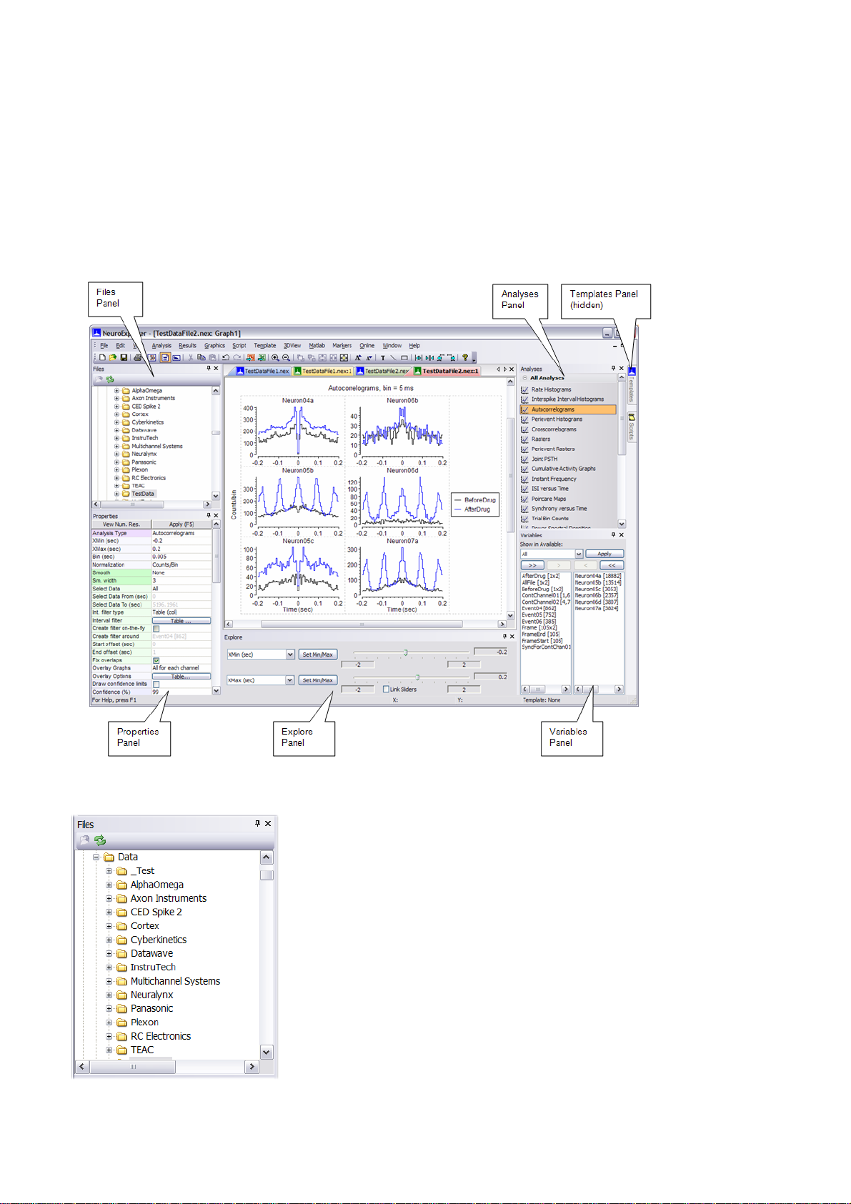
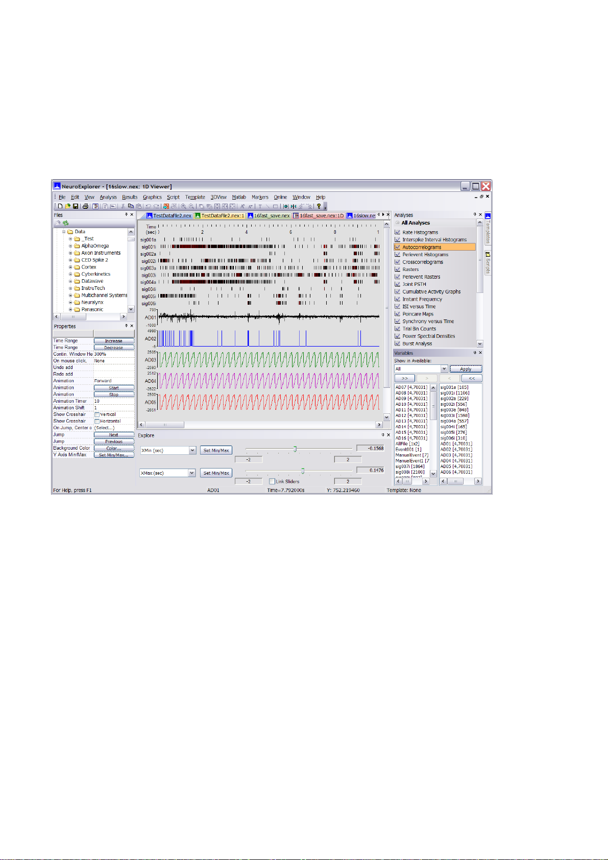
1.3. NeuroExplorer Screen Elements

NeuroExplorer user interface consists of the main window surrounded by several panels. These panels allow you to select files, select analyses and specify analysis properties. The figure below shows the default layout of NeuroExplorer window. Files, Properties, Analyses, Variables and Explore panels are visible and Templates and Scripts panels are hidden. To view a hidden panel, click at the panel tab or use View menu command.

You can reposition panels by dragging them with your mouse and you can save and restore window layouts using Window menu commands.

Files Panel

This view allows you to quickly browse through your data files. When you select (single-click) one of the data files, NeuroExplorer displays the file header information in the Properties panel. To open the

Page 12

data file, simply double-click the file name.

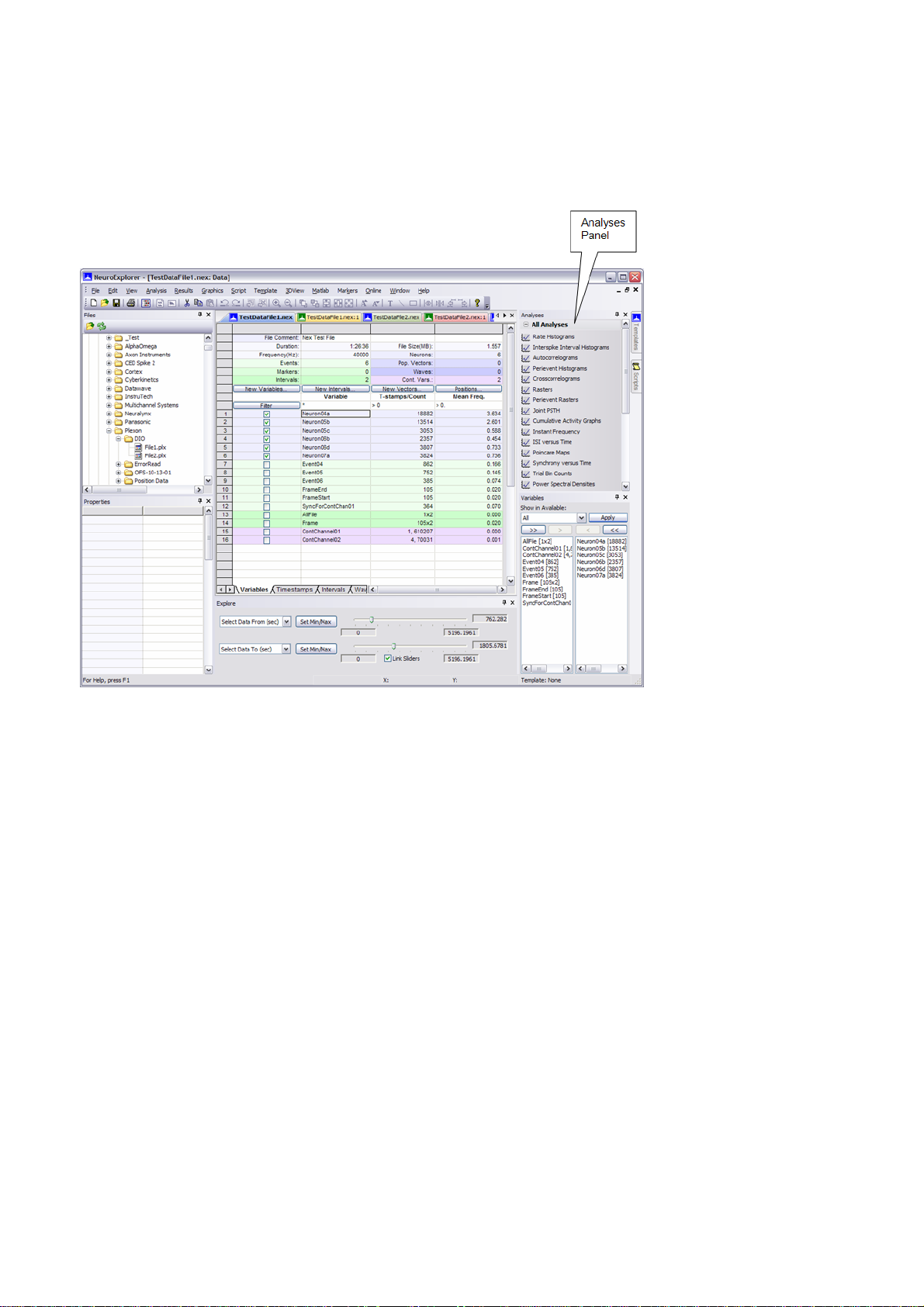
Analyses Panel

This view allows you to quickly select one of the analyses available in NeuroExplorer. To apply analysis to the active data file, click at the analysis name.

Properties Panel

The left column of the Properties Panel lists the names of adjustable parameters for the selected object. The right column contains various controls that can be used to change the parameter values. To apply the changes, press the Apply button or hit the F5 key.

Templates Panel

The Templates View can be used to quickly execute an Analysis Template. Double-click the template name and the corresponding template will be immediately executed.

You can create subfolders in your template directory and then NeuroExplorer will allow you to navigate through the templates tree within the Templates View.

Page 13

Variables Panel

You can analyze all the variables in your data file, a subset of the variables, or may be just one variable. Variables Panel allows you to quickly select and deselect the variables used for analysis:

The left column shows the variables that are not currently selected; the right column shows the selected variables. To move variables from column to column, first select them, then press ">" (Select) or "<" (Deselect) buttons.

Scripts Panel

This panel can be used to select a script to be executed. Double-click the script name to run the selected script.

You can create subfolders in your script directory and then NeuroExplorer will allow you to navigate through the scripts tree within the Scripts View.

Explore Panel

Page 14

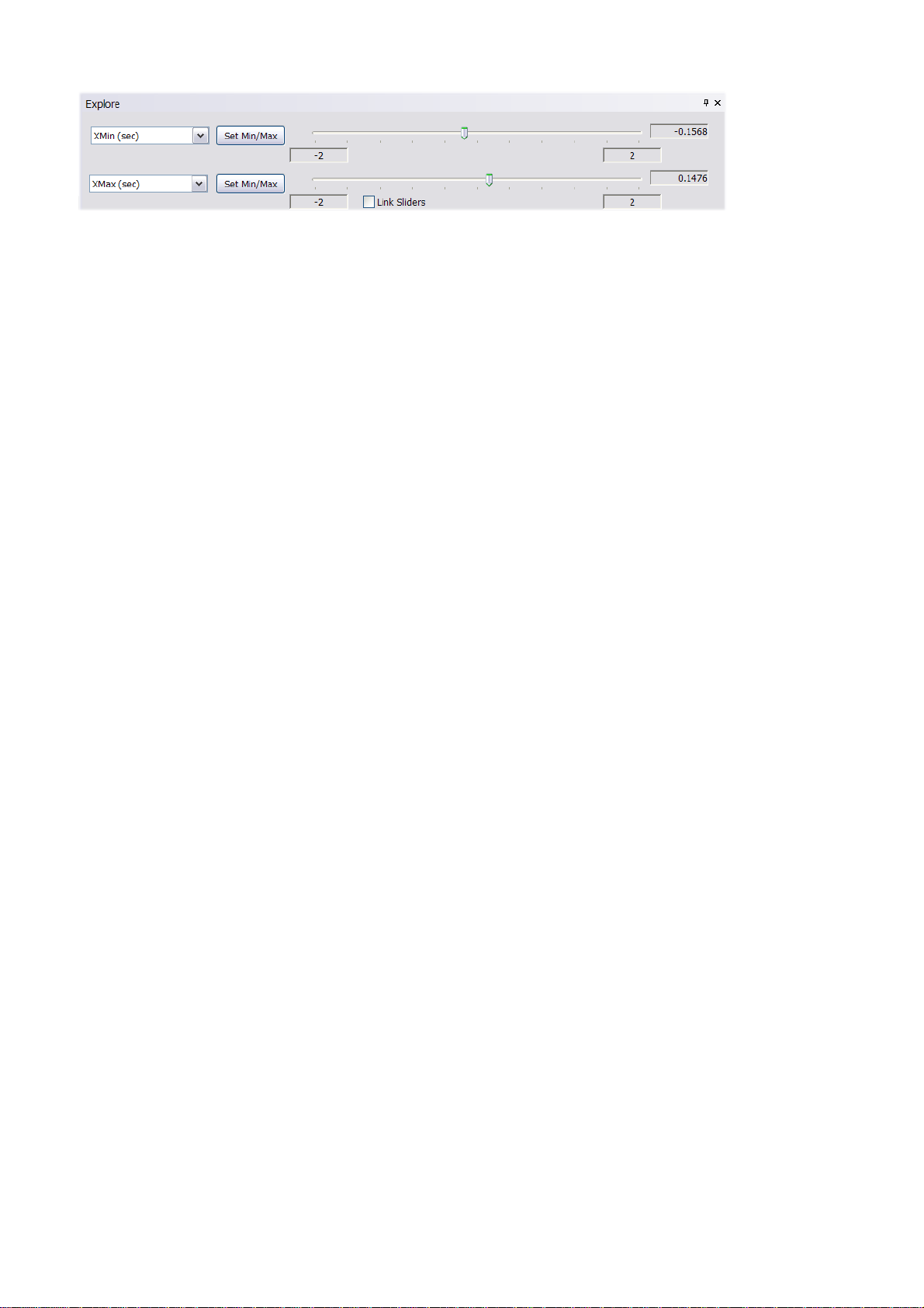
Explore panel allows you to quickly explore analysis parameter ranges. Select a parameter you want to explore from a list and drag a slider. NeuroExplorer will keep recalculating analysis with the new parameter values while you drag the slider, thus creating an “analysis animation”.

One of the best uses for this panel is to explore analysis properties over a sliding window within your file:

•

Specify Use Time Range using Analysis | Edit menu command, then Data Selection tab

•

Select ‘Select Data From’ and ‘Select Data To’ parameters in the list boxes of the Explore panel

•

Click on Link Sliders check box

Now, when you drag one of the sliders, the other one will follow allowing you to visualize analysis results over a sliding window in time.

Page 15

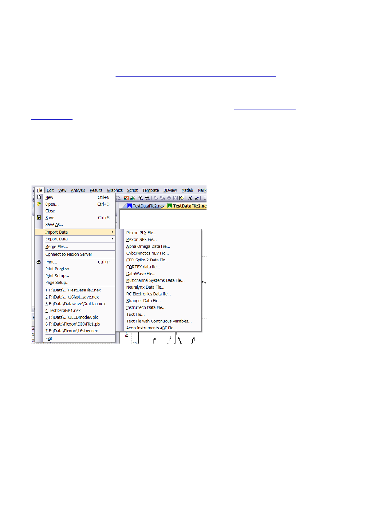
1.4. Opening Files and Importing Data

NeuroExplorer can read native data files created by popular data acquisition systems (Alpha Omega, CED Spike-2, Cortex, Blackrock Microsystems, DataWave, Multi Channel Systems, Neuralynx, Plexon, RC Electronics. See Importing Files Created By Data Acquisition Systems for more

information). NeuroExplorer can also import data from text files (see Importing Data from Text Files ). You can import the data from spreadsheets using the clipboard (see Importing Data from

Spreadsheets ).

NeuroExplorer has its own data format and by default saves the data in the binary file with the extension.nex.

To open a NeuroExplorer data file,

•

press File Open toolbar button , or

•

select File | Open... menu command.

To import data in any of the supported file formats, select the corresponding File | Import command:

You can also paste data directly into Data View. See Importing Data from the Text Files and

Importing Data from Spreadsheets for more information.

Page 16

1.5. Importing Files Created by Data Acquisition Systems

NeuroExplorer can read native data files created by popular data acquisition systems (Alpha Omega, CED Spike-2, Cortex, DataWave, Blackrock Microsystems, Multi Channel Systems, Neuralynx, Plexon, RC Electronics).

Since NeuroExplorer does not provide spike sorting capabilities yet, it is assumed that you have already sorted (clustered) the waveforms.

Alpha Omega Files

NeuroExplorer can import Alpha Omega MAP, ISI, NDA, MAT and LSM files. All the spike trains, DIO events and continuous variables are imported. The waveforms can be imported as an option (see File

Import Options below).

Blackrock Microsystems Files

NeuroExplorer can import Blackrock Microsystems NEV files. All the spike trains and DIO events Analog channels can be imported as an option. The waveforms are imported when using Neuroshare DLL to import NEV files.

DataWave Files

NeuroExplorer can import both Discovery and Workbench files. In general, all the sorted spike trains, DIO events and trial descriptors are imported. The waveforms are not imported. Analog channels can be imported as an option (see Options below).

The following UFF types are imported from the Discovery files:

S, E and U UFF types are imported as spike trains B UFF type records are imported as events T UFF type records are imported as markers P (position) UFF type records are imported as 4 continuous variables.

The following record types are imported from the Workbench files: Analysis records (with appropriate subtypes) are imported as spike trains Event records are imported as events Trial records are imported as markers

CED Spike-2 Files

NeuroExplorer can import Spike-2 *.smr files. All the sorted spike trains, events and markers are imported. The waveforms are not imported. Analog (Adc) channels can be imported as an option (see

File Import Options below).

Plexon Files

NeuroExplorer can read *.plx and *.ddt Plexon files. All the sorted spike trains and external events are imported. The waveforms are not imported. Analog (slow) channels can be imported as an option (see File Import Options below).

RC Electronics Files

NeuroExplorer can import both 12-bit RC Electronics files and 16-bit DATAMAX files. Since the current version of NeuroExplorer stores all the data in RAM, NeuroExplorer can import only relatively small (about the size of RAM on your PC) RC Electronics files.

Page 17

Multi Channel Systems Files

NeuroExplorer can import standard MCS data files. All the sorted spike trains and external events are imported. The waveforms are not imported. Analog channels can be imported as an option (see File

Import Options below).

Neuralynx Files

NeuroExplorer can import Neuralynx data files (tt*.dat, se*.dat, etc.) as well as the files created by MClust spike sorter (*.t files). All the sorted spike trains are imported. External events are imported as markers. Analog channels and waveforms can be imported as an option (see File Import Options

below).

File Import Options

The file import options can be set in the Data Import dialog (use View | Data Import Options menu command to invoke the dialog).

Page 18

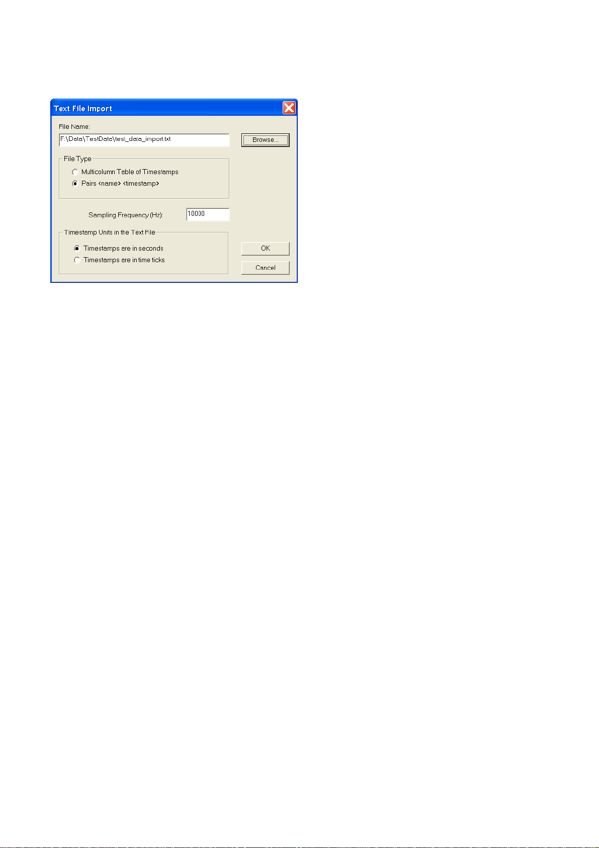
1.6. Importing Data from Text Files

You can specify text import options in the Text Import dialog:

Sampling Frequency - this parameter defines the internal representation of the timestamps that NeuroExplorer will use for this file. Internally, the timestamps are stored as integers representing the number of time ticks from the start of the experiment. The time tick is equal to

1./ Sampling_Frequency

Timestamp Units - this parameter defines how the numbers representing the timestamps are treated by NeuroExplorer. If the timestamps are in time ticks, they are stored internally exactly as they are in the text file. If the timestamps are in seconds, NeuroExplorer converts them to time ticks:

Internal_Timestamp = Timestamp_In_Seconds * Sampling_Frequency

NeuroExplorer can import timestamped data stored in the following text formats:

1. Multicolumn table of timestamps

In this format, each column in the text file contains the timestamps of a neuron. The first element in each column is a neuron name, that is the first line of the file contains names of all the variables.

Each name should be less than 64 characters long and should contain only letters, digits or the underscore sign. The first character of the name should be a letter. The timestamps are numbers representing the neuron firing time (or event time) in seconds or in time ticks. NeuroExplorer assumes that the columns are separated by tabs.

Here is an example of a text file with the timestamps represented in seconds:

Neuron01 Neuron02

0.01 0.001

0.3 0.05

0.5 0.1

0.4

0.6

NeuroExplorer can also export data in this format (use File | Save Data | As a Text File menu command).

2. Pairs <name> <timestamp>

The text file in this format should contain the pairs of the type <name><timestamp> where <name> is a character string that is less that 64 characters long and contains only letters, digits and

the underscore sign. The first character of the name should be a letter. If the number is used for the

Page 19

name, NeuroExplorer will add "event" at the beginning of the name. <timestamp> is a number representing the neuron firing time (or event time) in seconds or in time

ticks. Here is an example of a text file with the timestamps represented in seconds:

Neuron01 0.01 Neuron01 0.3 Neuron02 0.001 Neuron02 0.05 Neuron01 0.5 Neuron02 0.1 Neuron02 0.4

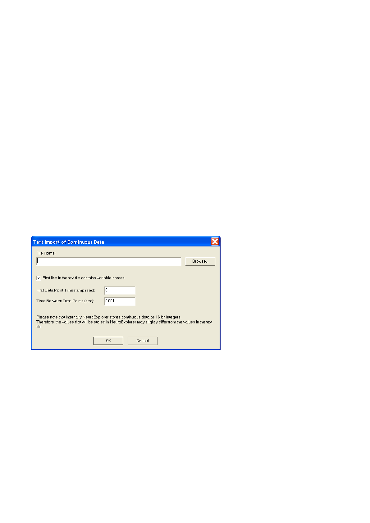
3. Multicolumn text files with continuous data

NeuroExplorer can also import continuous data from a multicolumn text file where each column corresponds to a continuous variable:

ContChannel1 ContChannel2

114.74609 -63.47656

56.15234 -358.88672

-187.98828 -63.47656

-48.82813 388.18359

-26.85547 285.64453

The columns may be separated by any number of spaces, tabs or commas. When you import continuous data from text files, the following dialog is shown:

First line contains variable names – if this option is selected, the fields of the first line of the text file are used as variable names. The second line in the file is the first row of data.

First Data Point Timestamp specifies the timestamp of the first data point in each continuous variable.

Time Between Data Points specifies the time step used in calculation of the timestamp for each row of data. For data row N (N = 1, 2, …) in the text file, the timestamp is calculated using the following formula:

DataRowTimestamp = FirstDataPoint + (N-1)*TimeBetweenDataPoints

1.7. Importing Data from Spreadsheets

Page 20

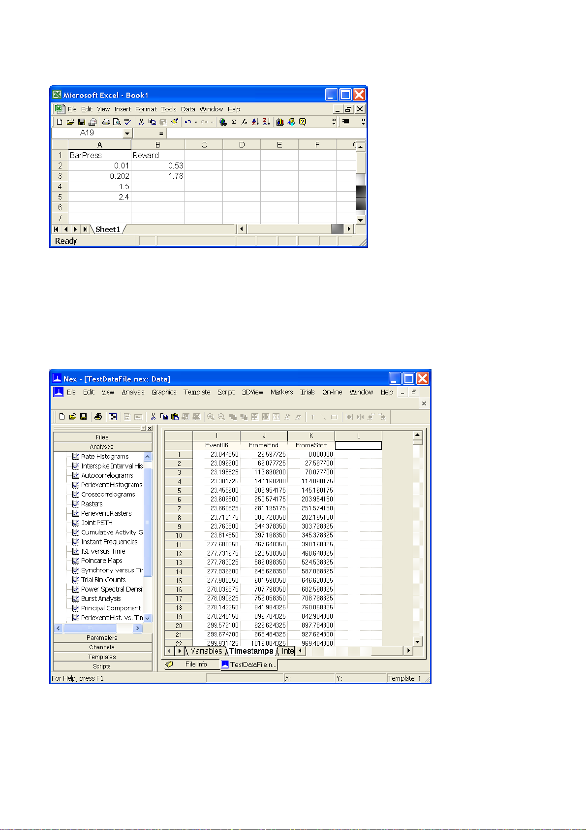
Timestamped data can be pasted directly into the NeuroExplorer data table. To paste the following two timestamped variables (BarPress and Reward) from a spreadsheet to NeuroExplorer:

In Excel:

•

Using the mouse, select the cell range with both variables (A1 to B5)

•

Select Edit | Copy menu command

In NeuroExplorer:

•

Select Data view of the file in NeuroExplorer

•

Select the Timestamps tab of the Data view

•

Scroll the timestamps window to the right and select the topmost cell of the empty column:

Select Edit | Paste menu command. NeuroExplorer will create two new Event variables and add them to the file. You need to save the file (use File | Save or File | SaveAs menu command) to make this change permanent.

Page 21

1.8. Importing Data from Matlab

You can create spike trains (1xN or Nx1 matrices with timestamps in seconds) or continuous variables in Matlab and transfer them to NeuroExplorer on the fly. Here is how to do this:

•

Select File | New menu command.

•

Select Matlab | Get Data From Matlab... | Open Matlab As Engine menu command. NeuroExplorer will open Matlab as engine.

•

In opened Matlab, run your Matlab scripts and create (or load from file) spike train variables or continuous variables.

•

To import timestamp variables, in NeuroExplorer, select Matlab | Get Data From Matlab... | Get Timestamp Variables... menu command. NeuroExplorer will open a dialog with the list of

available Matlab variables.

•

In the dialog, select the variables you want to transfer to NeuroExplorer and press OK.

•

To import continuous variables, in NeuroExplorer, select Matlab | Get Data From Matlab... | Get Continuous Variables... menu command. NeuroExplorer will open a dialog with the list of

available Matlab variables.

•

In the dialog, select one of the variables you want to transfer to NeuroExplorer and press OK. NeuroExplorer will open a dialog where you will specify the variable options.

Page 22

1.9. Reading and Writing NeuroExplorer Data Files

NeuroExplorer Data file has the following structure: file header variable header 1 variable header 2 ... data for variable i data for variable j ... Each variable header contains the size of the array that stores the variable data as well as the

location of this array in the file. The pseudo-code for reading NeuroExplorer data file looks like this:

open file in binary mode

read file header

for each variable read variable header end for

for each variable header seek to the file offset specified in the variable header read variable data end for  

The C++ source code of the program that reads and writes NeuroExplorer data files is available at NeuroExplorer web site:

http://www.neuroexplorer.com/updates/HowToReadAndWriteNexFiles.zip

There is also a Matlab script that reads NeuroExplorer data files:

http://www.neuroexplorer.com/updates/HowToReadNexFilesInMatlab.zip

Page 23

1.10. 1D Data Viewer

NeuroExplorer provides a window that displays graphically all the selected variables. To open this window, use View | 1D Data Viewer Window menu command.

You can also use 1D view to manually add events to the data file. Simply press the left mouse button when the pointer is in the 1D view and NeuroExplorer will add a new timestamp to the variable ManualEvent. You can also specify to what Event variable NeuroExplorer will add timestamps when you click in 1D view (use On mouse click parameter in the Properties Panel).

Mouse wheel can be used to quickly navigate in 1D View:

•

Click in 1D View so set 1D View as an active window in NeuroExplorer

•

Press Shift and rotate mouse wheel to shift 1D View horizontally

•

Press Ctrl and rotate mouse wheel to increase time range (zoom out) and decrease time range (zoom in)

Page 24

1.11. Analyzing Data

NeuroExplorer provides a variety of spike train analysis methods. Each method has a number of parameters and options. You can apply any available analysis by clicking at the corresponding analysis in the Analyses Panel (you can also use Analysis | Select Analysis menu commands):

After you click at one of the analysis items, NeuroExplorer will open a dialog that will allow you to edit the analysis parameters. When you click OK in this dialog, NeuroExplorer will apply the specified analysis to all the selected variables.

Any combination of analysis parameters and options (together with all the graphics options) can be saved as a template. To save the current configuration as a template, right-click in the Graph Window and select Save As New Template menu command. The template names are shown in the Templates view of the control panel.

When you open a new data file, you can simply double-click on the template name to apply the specific analysis with the selected parameter values.

Page 25

1.12. Selecting Variables for Analysis

NeuroExplorer can analyze at once any group of variables in the file. To select the variables to be analyzed, use one of the following methods:

•

Select the variables using the Variable Panel (see How to select variables using Variables Panel )

•

Select the variables using Analysis | Select Variables menu command. This command will invoke the Variable Selection dialog similar to Variables Panel.

•

Select the variables directly in the Variables Window by using the check boxes located next to the variable names. Please note that variable selection in Variables Window is applied only

when a new Graph Window or 1D View is created. To change the list of selected variables in existing Graph Window, use Variables Panel or Analysis | Select Variables menu command. See How to Select Variables for Existing Analysis Window for details.

Page 26

1.13. How to Select Variables for Existing Window

Variables selected in the Variables spreadsheet of data window are used to populate variables lists of new analysis windows.

If you would like to change the list of variables for existing analysis window, please follow these steps:

•

Click anywhere in analysis window to activate it

•

If Variables panel is visible, make changes in selected variables list ( how? ) and press Apply button:

•

If Variables panel is hidden, click at panel tab to open it:

Page 27

•

Make changes in selected variables list ( how to make changes? ) and press Apply button

•

If Variables panel or its tab is not visible, use View | Variables Panel menu command

Page 28

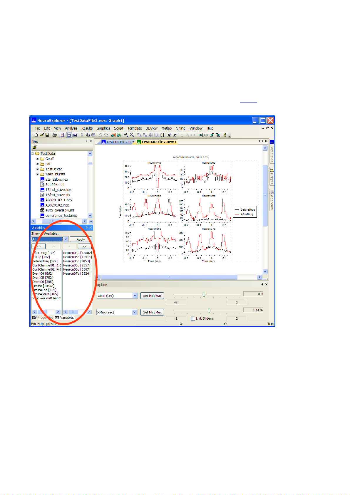
1.14. How to Select Variables in Variables Panel

Select variables for analysis by moving them from the left (available) to the right (selected) list box. In the figure below, 6 variables (Neuron04a, Neuron05b, ..., Neuron07a) are selected for analysis:

To move variables from one listbox to another:

Select variables using the mouse (in the figure above two variables in Available listbox are

•

selected -- ContChannel01 and ContChannel02) Press one of four buttons just above the listboxes

•

The drop-down box above the buttons can be used to specify what kind of variables are shown in the available window:

Page 29

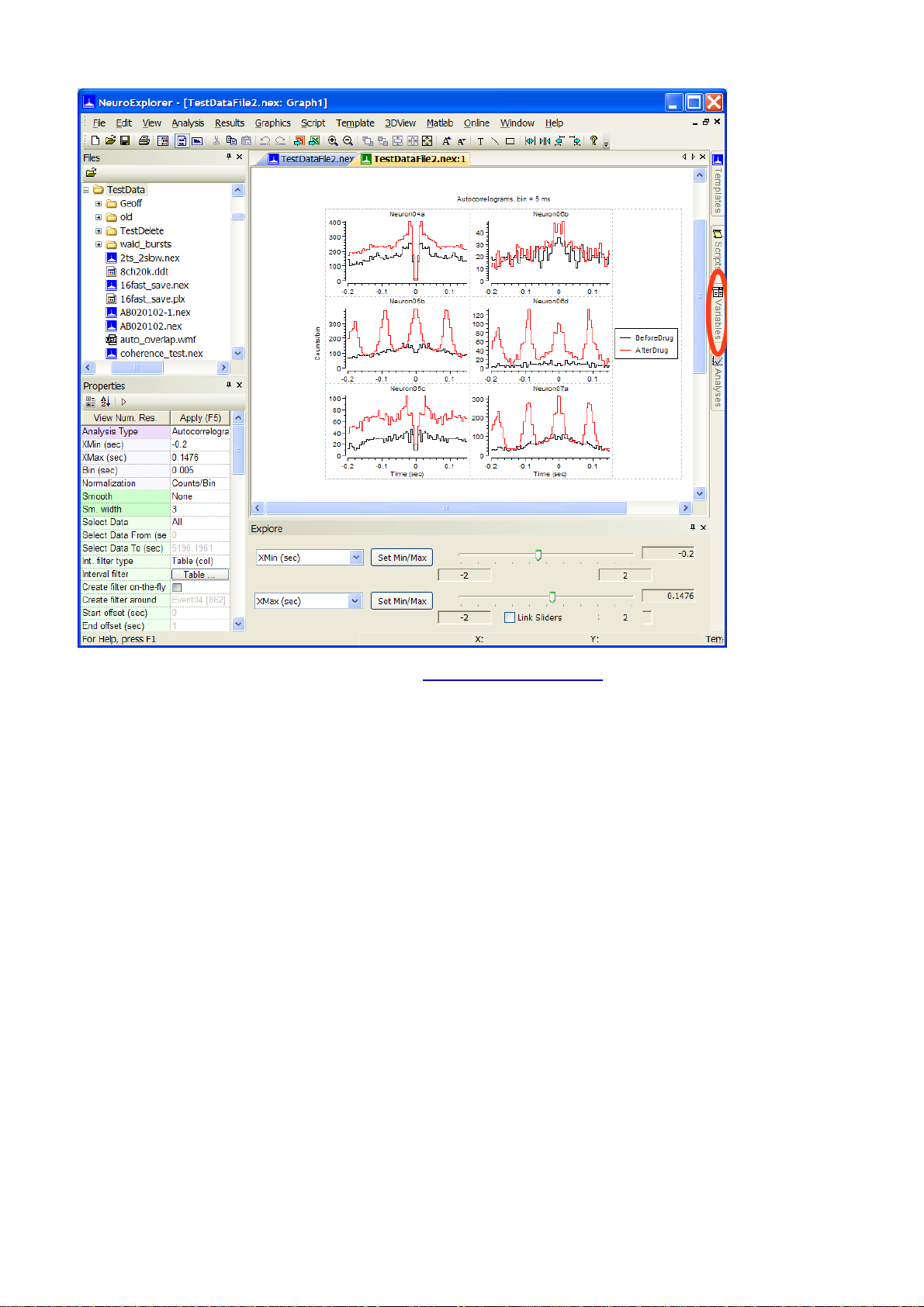
1.15. Adjusting Analysis Properties

There are several methods to adjust the analysis parameters:

•

Use Analysis | Edit Parameters menu command to invoke the Analysis Parameters dialog

•

Right-click in the Graph Window and choose Analysis Parameters item in the floating menu

The floating menu is the fastest way to adjust any analysis or graphics parameters. Double-click (or right-click) anywhere in the Graph Window to invoke this menu:

This menu allows you to go directly to analysis properties, graph properties, axes properties, etc. You can also use it to save the current template and save the current analysis configuration as a new template.

•

Single-click in the graph area of the Graph Window and adjust parameters in the Properties Panel:

Page 30

1.16. Analysis Templates

In any analysis in NeuroExplorer, you can adjust a large number of parameters:

•

Analysis type (Rate Histograms, IIH, etc)

•

Analysis parameters (Bin, XMin, XMax, etc.)

•

Graph parameters (graph type, graph color, grid lines, etc)

•

Parameters of X and Y axes (labels, numerics, lines, colors, etc.)

•

Graph and page labels and other elements

NeuroExplorer allows you to save all these parameters so that when you open another data file, you can easily reproduce exactly the same analysis with the same axes, labels and so on.

The set of all the analysis parameters is called the Template. To save the current analysis as a template:

•

Select the menu command Template | Save As New Template, or

•

Right-click in the graph and choose the Save As New Template command in the floating menu.

After you saved the template, the name of the template appears in the Templates Window (see

NeuroExplorer Screen Elements ). You can apply the template to the currently opened file by double-

clicking the template name in the Templates Window. NeuroExplorer stores template files in Windows Application Data directory:

C:\Documents and Settings\All Users\Application Data\Nex Technologies\NeuroExplorer\Templates

under Windows XP, or C:\Application Data\Nex Technologies\NeuroExplorer\Templates under Vista or Windows 7.

Page 31

1.17. Numerical Results

To view the analysis numerical results, select View | Numerical Results menu command. You can also press the "View. Num. Res." button in the upper-left corner of the Properties Panel:

NeuroExplorer will open Numerical Results Window:

Note that the window has two Excel-style sheets -- the Results sheet and the Summary sheet. The Results sheet usually contains the bin counts or other histogram values. The Summary sheet contains summary statistics of the analyses such as the mean firing rate, the number of spikes used in the analysis, etc.

Page 32

1.18. Post-processing

For the histogram-style analyses, NeuroExplorer has an optional Post-Processing analysis step. You can select post-processing options using Post-processing tab in the Analysis Parameters dialog (double-click in Graph window and select Analysis Parameters menu item):

You can smooth the resulting histogram with Gaussian or Boxcar filters. You can also add bin information to the matrix of results. See Post-processing Options for details.

See Saving Results as Power Point Slides, Working with Matlab and Working with Excel for more information on NeuroExplorer post-processing options.

1.19. Saving Results as Power Point Slides

NeuroExplorer version 3 provides a powerful new option that allows you to save graphics, analysis parameters and your annotations as slides in a Power Point Presentation.

To save your results to Power Point, press a toolbar button , or select Graphics | Export Graphics | Export to Power Point menu command. NeuroExplorer will start Power Point if Power Point is not running, and will add a new slide to the specified presentation file. The slide will contain:

Copy of the graphics

•

Analysis parameters

•

Your comment

•

Data file name

•

Current date and time

•

Page 33

Power point presentation then becomes your lab notebook where you can save your NeuroExplorer analysis results:

Page 34

1.20. Working with Matlab

NeuroExplorer can interact with Matlab via COM interface using Matlab as a powerful postprocessing engine. Matlab can also control NeuroExplorer and exchange data with NeuroExplorer via NeuroExplorer COM interfaces. See COM/ActiveX Interfaces for details.

Immediately after calculating the histograms, NeuroExplorer can send the resulting matrix of histograms to Matlab and then ask Matlab to execute any series of Matlab commands.

Use the Matlab tab in the Analysis parameters dialog to specify the matrix name and the Matlab command string.

NeuroExplorer can also send its data variables to Matlab. To transfer the variables to Matlab, use Matlab | Send Selected Variables to Matlab menu command.

In general, a continuous variable may contain several fragments of data. Each fragment may be of a different length. NeuroExplorer does not store the timestamps for all the A/D values since they would use too much space. Instead, for each fragment, it stores the timestamp of the first A/D value in the fragment and the index of the first data point in the fragment. Therefore, for a continuous variable (named ContVar1), the following 3 vectors will be created in Matlab:

•

ContVar1 - vector (or matrix with 2 columns) of all A/D values in milliVolts. If "Optimize transfer

for small amounts of data" is selected in View | Options | Matlab, Contvar1 is a matrix with 2 columns: the first column contains A/D values in millivolts, the second column contains timestamps in seconds.

•

ContVar1_ts - vector of fragment timestamps in seconds. Each timestamp is for the first A/D

value of the fragment.

•

ContVar1_ind - array of indexes. Each index is the position of the first data point of the

fragment in the A/D array. If ContVar1_ind (2) = 201, it means that the second fragment is ContVar1 [201], ContVar1 [202], etc.

•

ContVar1_ts_step - digitizing step in seconds.

You can generate all the timestamps for continuous variable using this Matlab script:

function [ ts ] = MakeTs( fragmentInd, fragmentTs, numValues, step ) % MakeTs: makes timestamps for continuous variable based on the fragment % information % INPUT: fragmentInd - vector of fragment indexes % fragmentTs - vector of fragment timestamps % numValues - total number of values in all fragments % step - digitizing step of continuous variable % % Example: NeuroExplorer sent continuous variable FP01 via file transfer % The following values were sent: % FP01 - vector of continuous values % FP01_ind - fragment indexes % FP01_ts - fragment timestamps % FP01_ts_step - digitizing step % % to generate all timestamps for FP01, use: % % ts = MakeTs(FP01_ind, FP01_ts, size(FP01,1), FP01_ts_step); % ts = []; numFr = size(fragmentTs); % add fake index for the last fragment fragmetInd = [fragmentInd; numValues+1]; for i=1:numFr valuesInFragment = fragmetInd(i+1)-fragmentInd(i);

Page 35

ts = [ts; (fragmentTs(i) + (0:(valuesInFragment-1))*step)']; end end

You can also import timestamped and continuous variables directly from Matlab. See Importing Data

From Matlab for details.

1.21. Working with Excel

The easiest way to transfer data and numerical results from NeuroExplorer to Excel is by using the clipboard:

•

select a range of cells in NeuroExplorer and choose Edit| Copy

•

switch to Excel and use the Paste command (select a cell and choose Edit | Paste ).

NeuroExplorer can also send numerical results directly to Excel. There two ways to send the results to Excel:

•

Use Send to Excel button on the toolbar or menu command File | Save Numerical Results | Send Results to Excel

•

Use Excel tab in the Analysis Parameters dialog to specify what to transfer to Excel and the location of the top-left cell for the data from NeuroExplorer.

Page 36

1.22. Saving Graphics

NeuroExplorer can save the contents of the Graph window in a file using the Windows Metafile format. The file can then be opened in any program that can use the.wmf format files (a word processor, graphics editor, etc.).

To save the graphics in a metafile, use File | Save Graphics menu command. You can also copy the graphics to the clipboard and then paste in another application. To copy the

graphics, single-click in the graph area and then select Edit | Copy menu command. See also Saving Results as Power Point Slides.

Page 37

2. Analysis Reference

This section, NeuroExplorer Analysis Reference, describes general pre-processing and postprocessing analysis options, analysis parameters and computational algorithms used in analyses.

•

Data Types

•

Data Selection Options

•

Post-Processing Options

•

Matlab Options

•

Excel Options

•

Confidence Limits for Perievent Histograms

•

Rate Histograms

•

Interspike Interval Histograms

•

Autocorrelograms

•

Perievent Histograms

•

Crosscorrelograms

•

Rasters

•

Perievent Rasters

•

Joint PSTH

•

Cumulative Activity Graphs

•

Instant Frequency Graphs

•

Interspike Intervals vs Time

•

Poincare Maps

•

Spike Distance vs Time

•

Trial Bin Counts

•

Power Spectral Densities

•

Burst Analysis

•

Principal Component Analysis

•

Perievent Histograms vs. Time

•

Correlations with Continuous Variables

•

Regularity Analysis

•

Place Cell Analysis

•

Reverse Correlation

•

Epoch Counts

•

Coherence Analysis

Page 38

2.1. Data Types

NeuroExplorer supports several data types -- spike trains, behavioral events, time intervals, continuously recorded data and other data types. The topics in this section describe the data types used in NeuroExplorer, list the properties of data types, and show how to view and modify various data types in NeuroExplorer.

2.1.1. Spike Trains

In NeuroExplorer, the most commonly used data type is a spike train. A spike train in NeuroExplorer does not contain the spike waveforms, it represents only the spike timestamps (the times when the spikes occurred). A special Waveform data type is used to store the spike waveform values.

Events are very similar to spike trains. The only difference between spike trains and events is that

spike trains may contain additional information about recording sites, electrode numbers, etc. (for example, spike trains contain positions of neurons used in the 3D activity "movie" ).

Internally, the timestamps are stored as 32-bit signed integers. These integers are usually the timestamps recorded by the data acquisition system and they represent time in the so-called time ticks. For example, the typical time tick for the Plexon system is 25 microseconds, so an event recorded at 1 sec will have the timestamp equal to 40000.

Limitations

The maximum number of timestamps (in each spike train) in NeuroExplorer is 2,147,483,647. In reality, the limiting factor is the amount of virtual memory on your machine, since the timestamps of all the variables of a data file should fit into memory. NeuroExplorer requires that in each spike train all the timestamps are in ascending order, that is

timestamp[i+1] > timestamp[i] for all i. NeuroExplorer also requires that timestamp[i] >= 0 and timestamp[i] < 2,147,483,647 for all i. The upper timestamp limit defines the maximum experiment length that can be safely analyzed in

NeuroExplorer. Thus, for the standard Plexon setup, the maximum duration of the experiment is 2147483647/40000 seconds, or 14 hours and 54 minutes.

Timestamped Variables in NexScript

You can get access to any timestamp in the current file. For example, to assign the value 0.5 (sec) to the third timestamp of the variable DSP01a, you simply write:

doc = GetActiveDocument() doc.DSP01a[3] = 0.5

Viewers

You can view the timestamps of the selected variables in graphical display ( View | 1D Data Viewer menu command):

Page 39

Numerical values of the timestamps (in seconds) are shown in the Timestamps sheet of the Data view:

2.1.2. Events

Event data type in NeuroExplorer is used to represent the series of timestamps recorded from external devices (for example, stimulation times recorded as pulses produced by the stimulus generator). Event data type stores only the times when the external events occurred. A special

Marker data type is used to store the timestamps together with other stimulus or trial information.

Events are very similar to spike trains. The only difference between spike trains and events is that spike trains may contain additional information about recording sites, electrode numbers, etc.

Internally, event timestamps are represented exactly as Spike Train timestamps. See Spike Trains for more information about the timestamps in NeuroExplorer.

Creating Event Variables

You can add events to the data file using Copy | Paste command in the Timestamps view (see

Importing Data from Spreadsheets for details).

You can also create additional events based on the events in the data file. Use Edit | Operations on

Data Variables menu command and then select one of the operations in the Operations dialog.

2.1.3. Intervals

Intervals are usually used in NeuroExplorer to select the data from a specified time periods (see Data

Selection Options for details).

Each interval variable can contain multiple time intervals. For example, the Frame variable in the following figure has two intervals:

Page 40

Creating Interval Variables

You can create intervals in NeuroExplorer using Edit | Add Interval Variable menu command. You can also create intervals based on existing Event or Interval variables. Use Edit | Operations on

Data Variables menu command and then select one of the following operations: MakeIntervals MakeIntFromStart MakeIntFromEnd IntOpposite IntAnd IntOr IntSize IntFind

Burst analysis creates interval variables (one for each neuron) that contain all the detected bursts as

time intervals.

Interval Variables in NexScript

IntVar[i,1] gives you the access to the start of the i-th interval, IntVar[i,2] gives you the access to the end of the i-th interval.

For example, the following script creates a new interval variable that has two intervals: from 0 to 100 seconds and from 200 to 300 seconds:

doc = GetActiveDocument() doc.MyInterval = NewIntEvent(doc, 2)

doc.MyInterval[1,1] = 0. doc.MyInterval[1,2] = 100.

doc.MyInterval[2,1] = 200. doc.MyInterval[2,2] = 300.

Limitations

Internally, NeuroExplorer stores the beginning and the end of each interval as a timestamp (see

Spike Trains for more information about timestamps in NeuroExplorer).

Viewers

You can view the intervals of the selected variables in graphical display ( View | 1D Data Viewer menu command, see figure above).

The intervals (in seconds) are shown in the Intervals sheet of the Data view:

Page 41

2.1.4. Markers

Marker data type in NeuroExplorer is used to represent the series of timestamps recorded from external devices (for example, stimulation times recorded as pulses produced by the stimulus generator) together with other stimulus or trial information. Event data type stores only the times

when the external events occurred. NeuroExplorer creates Marker variables when it imports strobed events from Plexon data files, when

it imports Trial Descriptor Records from the Datawave files and when DIO events with flags are loaded from Alpha Omega files.

Viewers

You can view both the marker timestamps and additional marker information in the Markers tab of the Data window:

Extracting Events

Usually you will need to extract events with specific trial information from the marker variables. To do this, use Marker | Split... and Marker | Extract... menu commands.

For example, you may want to extract from the marker variable shown in the figure above only the markers with DIOValue 131 or 132. Marker | Extract... menu command will open the Extract dialog box in which you can specify multiple criteria for extracting events from the marker variable:

Page 42

2.1.5. Population Vectors

Population vectors in NeuroExplorer can be used to display the linear combinations of histograms in some of the analyses. For example, you can calculate perievent histograms for each individual neuron recorded in a data file. If you want to calculate the response of the whole population of neurons (that is, create an average PST histogram) you need to use a population vector.

Population vector assigns a weight to each spike train or event variable in the file. You can then use population vectors in the following analyses:

Rate Histograms

•

Perievent Histograms

•

Trial Counts

•

If you select the population vector for analysis and then run one of the three analyses listed above, the histogram corresponding to the population vector will be calculated as:

histogram_of_neuron_1 * weight_1 + histogram_of_neuron_2 * weight_2...

where the weights are defined in the population vector. For example, to calculate an average histogram for 6 neurons, the following population vector should be used:

Creating Population Vectors

You can create new population vectors in NeuroExplorer using Edit | Add Population Vector menu command.

Page 43

Principal Component Analysis creates a set of population vectors based on correlations between

activities of individual neurons.

2.1.6. Waveforms

The waveform data type is used in NeuroExplorer to store the spike waveform values together with the spike timestamps. The following figure shows the waveform variable sig006a_wf together with the corresponding spike train sig006a:

The waveform data may not be imported by default from the data files created by the data acquisition systems. Use View | Data Import Options menu command to specify which data types NeuroExplorer will import from the data files.

The waveform variables can be used in the following analyses:

•

Rate Histograms

•

Rasters

•

Perievent Histograms (instead of PST, NeuroExplorer calculates spike-triggered average for a waveform variable)

Viewers You can view the waveforms of the selected variables in the graphical display ( View | 1D Data

Viewer menu command, see figure above).

Numerical values of the waveforms and their timestamps are shown in the Waveforms sheet of the Data view.

To select a different waveform variable, click in the cell located in the row 1 of the Variable column (the cell shows sig001i_wf in the figure above).

Waveform values are shown in columns labeled 1, 2, etc.

Page 44

2.1.7. Continuously Recorded Data

The continuous data type is used in NeuroExplorer to store the data that has been continuously recorded (digitized).

The following figure shows continuous variable AD01 together with the spike train sig001a:

Continuous data may not be imported by default from the data files created by the data acquisition systems. Use View | Data Import Options menu command to specify which data types NeuroExplorer will import from the data files.

Continuous variables can be used in the following analyses:

•

Rate Histograms

•

Rasters

•

Perievent Histograms (instead of PST, NeuroExplorer calculates the spike-triggered average for a continuous variable)

•

Perievent Rasters (NeuroExplorer shows the values of continuous variable using color)

•

Spectral Densities

•

Correlations with Continuous Variable

•

Coherence Analysis

Limitations

Internally, each data point of the continuous variable is stored as a 2-byte integer. The maximum number of values (in each continuous variable) in NeuroExplorer is 2,147,483,647. In reality, the limiting factor is the amount of virtual memory on your machine, since all the values should fit into virtual memory.

Viewers

You can view continuous variables in the graphical display ( View | 1D Data Viewer menu command, see figure above).

Numerical values of the continuous variables are shown in the Continuous sheet of the Data view.

Page 45

2.2. Data Selection Options

Before performing the analysis, NeuroExplorer can select the timestamped events that are inside the specified time intervals:

For example, you may want to analyze only the first 10 minutes of the recording session. To do this, choose the Data Selection tab in the Analysis Parameters dialog, click Use only the data from the following time range and specify From and To parameters in seconds:

You can also choose an interval variable (at the bottom of the Data Selection page) as an additional data filter. NeuroExplorer then will select data from one or more time intervals as specified by the interval variable.

Some analyses (Perievent Histograms, Perievent Rasters and Crosscorrelograms) allow you to specify several interval filters, so that a different filter will be used for a column or for a row of graphs.

Page 46

2.3. Post-Processing Options

For the histogram-style analyses, NeuroExplorer has an optional Post-processing analysis step. You can select post-processing options using Post-processing tab in the Analysis Parameters dialog.

(double-click in the Graph window and select Analysis Parameters menu item):

You can smooth the resulting histogram with Gaussian or Boxcar filters. The boxcar filter is a filter with equal coefficients. If f[i] is i-th filter coefficient and w is the filter width,

then

f[i] = 1/w for all i

Thus for the filter of width 3, the boxcar filter is

f[-1] = 0.33333, f[0] = 0.33333, f[1] = 0.33333.

and the smoothed histogram sh[i] is calculated as

sh[i] = f[-1]*h[i-1] + f[0]*h[i] + f[1]*h[i+1]

where h[i] is the original histogram. The Gaussian filter is calculated using the following formula:

f[i] = exp(-i*i/sigma)/norm, i from -2*d to 2*d

where

d = ( (int)w + 1 )/2 sigma = -w * w * 0.25 / log(0.5) norm = sum of exp( -i * i / sigma), i from -2*d to 2*d

The parameters of the filter are such that the width of the Gaussian curve at half the height equals to the specified filter width. Please note that for the Gaussian filter, width of the filter (w) can be a noninteger. For example, w can be 3.5.

See Matlab Options and Excel Options for more information on NeuroExplorer post-processing capabilities.

Page 47

2.4. Matlab Options

NeuroExplorer can interact with Matlab via COM interface using Matlab as a powerful postprocessing engine. Immediately after calculating histograms, NeuroExplorer can send the resulting matrix of histograms to Matlab and then ask Matlab to execute any series of Matlab commands.

Use the Matlab tab in the Analysis parameters dialog to specify the matrix name and the Matlab command string.

2.5. Excel Options

NeuroExplorer can send numerical results directly to Excel. There are two ways to send the results to Excel:

•

Use Send to Excel button on the toolbar or menu command File | Save Numerical Results | Send Results to Excel

•

Use Excel tab in the Analysis Parameters dialog to specify what to transfer to Excel and the location of the top-left cell for the data from NeuroExplorer.

Page 48

2.6. Confidence Limits for Perievent Histograms

If the total time interval (experimental session) is T (seconds) and we have N spikes in the interval, then the neuron frequency is:

F = N/T Several options how to calculate neuron frequency F are available. See Options below. Then if the spike train is a Poisson train, the probability of the neuron to fire in the small bin of the size

b (seconds) is P = F*b The expected bin count for the perievent histogram is then: C = P*NRef, where NRef is the number of the reference events. The value C is used for drawing the Mean Frequency in the Perievent Histograms and Cross- and

Autocorrelograms. The confidence limits for C are calculated using the assumption that C has a Poisson distribution.

Assume that a random variable S has a Poisson distribution with parameter C. Then the 99% confidence limits are calculated as follows:

Low Conf. = x such that Prob(S < x) = 0.005 High Conf. = y such that Prob(S > y) = 0.005 If C < 30, NeuroExplorer uses the actual Poisson distribution Prob(S = K) = exp(-C) * (C^K) / K!, where C^K is C to the power of K, to calculate the confidence limits. If C>= 30., the Gaussian approximation is used. For example, for 99% confidence limits: Low Conf. = C - 2.58*sqrt(C); High Conf.= C + 2.58*sqrt(C);

Reference

Abeles M. Quantification, smoothing, and confidence limits for single-units histograms. Journal of Neuroscience Methods. 5(4):317-25, 1982

Options

The following options to calculate neuron frequency F are available:

•

Use all file data. Here T is the total length of experimental session, N is the total number of spikes for a given neuron.

•

Use selected time range and interval filter. T is the length of all the time intervals used in analysis, N is the number of spikes within these intervals.

•

Use time intervals corresponding to prereference bins. This option only works for a stimulationtype data. For example, if you stimulate every second and calculate PSTH with XMin=-0.2, XMax=0.2, NeuroExplorer can easily distinguish the spikes before and after the stimulus. However, if you stimulate every 200 ms, the spikes before the second stimulus are also the spikes after the first stimulus, so you cannot distinguish the spikes that should be used to calculate the mean firing rate. The algorithm: for each reference event timestamp r, a time interval (r+XMin, r) is created (where XMin is PSTH or crosscorrelogram time axis minimum parameter; XMin should be negative). T is the length of all (r+XMin, r) intervals that do not overlap, N is the number of spikes in these intervals. If more than 5% of intervals overlap, F is set to zero.

Page 49

2.7. Cumulative Sum Graphs

Here is the algorithm that is used to draw optional cumulative sum graphs above the histograms. Suppose we have a histogram with bin counts bc[i], i=1,...,N. Cumulative Sum Graph displays the

following values cs[i]: for bin 1: cs[1] = bc[1] - A for bin 2: cs[2] = bc[1]+bc[2] - A*2 for bin 3: cs[3] = bc[1]+bc[2]+bc[3] - A*3, etc. The value of A depends on the selected Cumulative Sum option: A equals to average of all bc[i] if you select "Use all histogram" option A equals to average of all bc[i] for bins that are before zero on time scale if you select "Use preref as

base" option. If you use "Use all histogram" option, the value of the cumulative sum for the last bin is always zero:

sc[N] = bc[1]+bc[2]+...bc[N] - A*N, where A = (bc[1]+bc[2]+...bc[N])/N. NeuroExplorer displays 99% confidence limits for Cumulative Sum Graphs. Confidence limits for "Use

preref as base" option are proportional to square root of bin number. Calculations of confidence limits for "Use all histogram" option are not trivial. These calculations are

based on the formulas developed by the author of NeuroExplorer, Alexander Kirillov.

Page 50

2.8. Rate Histograms

Rate histogram displays firing rate versus time.

Parameters

Parameter Description XMin/XMax type An option on how XMin and XMax values are specified. XMin Time axis minimum in seconds. XMax Time axis maximum in seconds Bin Histogram bin size in seconds. Normalization Histogram units (Counts/Bin, Probability or Spikes/Second). See Algorithm

below.

Select Data If Select Data is From Time Range, only the data from the specified (by

Select Data From and Select Data To parameters) time range will be used

in analysis. See also Data Selection Options. Select Data From Start of the time range in seconds. Select Data To End of the time range in seconds. Smooth histogram An option to smooth the histogram after the calculation. See Post-

Processing Options for details.

Smooth Filter Width The width of the smooth filter. See Post-Processing Options for details. Add to Results / Bin left An option to add an additional vector (containing a left edge of each bin) to

the matrix of numerical results. Add to Results / Bin

middle Add to Results / Bin

right Send to Matlab An option to send the matrix of numerical results to Matlab. See also

Matrix Name Specifies the name of the results matrix in Matlab workspace. Matlab command Specifies a Matlab command that is executed after the numerical results

Send to Excel An option to send numerical results or summary of numerical results to

Sheet Name The name of the worksheet in Excel where to copy the numerical results.

An option to add an additional vector (containing a middle point of each

bin) to the matrix of numerical results.

An option to add an additional vector (containing a right edge of each bin)

to the matrix of numerical results.

Matlab Options.

are sent to Matlab.

Excel. See also Excel Options.

TopLeft Specifies the Excel cell where the results are copied. Should be in the form

CR where C is Excel column name, R is the row number. For example, A1

is the top-left cell in the worksheet.

Summary of Numerical Results

The following information is available in the Summary of Numerical Results

Column Description

Page 51

Variable Variable name. YMin Histogram minimum. YMax Histogram maximum. Spikes The number of spikes used in calculation. Filter Length The length of all the intervals of the interval filter (if a filter was used) or the

Algorithm

The time axis is divided into bins. The first bin is [XMin, XMin+Bin). The second bin is [XMin+Bin, Xmin+Bin*2), etc. The left end is included in each bin, the right end is excluded from the bin.

For each bin, the number of events in this bin is calculated. For example, for the first bin

bin_count = number of timestamps (ts) such that ts >= XMin and ts < XMin + Bin

If Normalization is Counts/Bin, no further calculations are performed. If Normalization is Spikes/Sec, bin counts are divided by Bin.

Page 52

2.9. Interspike Interval Histograms

Interspike interval histogram shows the conditional probability of a first spike at time t0+t after a spike at time t0.

Parameters

Parameter Description Min Interval Minimum interspike interval in seconds. Max Interval Maximum interspike interval in seconds. Bin Bin size in seconds. Normalization Histogram units (Counts/Bin, Probability or Spikes/Second). See Algorithm

below. Log Bins and X Axis An option to use Log10 interval scale (see Algorithm below for details). Bins per decade A bin size option if Log option is selected (see Algorithm below for details). Y Axis Limit (%) An option to "zoom in" small histogram values. This parameter specifies

the maximum of Y axis. If it is 100%, the Y axis maximum equals to the

maximum bin value. If it is, for example, 10%, Y axis maximum is set to

10% of the bin max and the small bin values have better visibility. Select Data If Select Data is From Time Range, only the data from the specified (by

Select Data From and Select Data To parameters) time range will be used

in analysis. See also Data Selection Options. Select Data From Start of the time range in seconds. Select Data To End of the time range in seconds. Int. filter type Specifies if the analysis will use a single or multiple interval filters. Interval filter Specifies the interval filter(s) that will be used to preselect data before

analysis. See also Data Selection Options. Create filter on-the-fly Specifies if a temporary interval filter needs to be created (and used to

preselect data). Create filter around Specifies an event that will be used to create a temporary filter. Start offset Offset (in seconds, relative to the event specified in Create filter around

parameter) for the start of interval for the temporary filter. End offset Offset (in seconds, relative to the event specified in Create filter around

parameter) for the end of interval for the temporary filter. Fix overlaps An option to automatically merge the overlapping intervals in the temporary

filter. Overlay Graphs An option to draw several histograms in each graph. This option requires

that Int. filter type specifies that multiple interval filters will be used (either

Table (row) or Table (col)). Smooth Option to smooth the histogram after the calculation. See Post-Processing

Options for details.

Smooth Filter Width The width of the smooth filter. See Post-Processing Options for details. Add to Results / Bin left An option to add an additional vector (containing a left edge of each bin) to

the matrix of numerical results.

Page 53

Add to Results / Bin middle

An option to add an additional vector (containing a middle point of each

bin) to the matrix of numerical results. Add to Results / Bin

right Send to Matlab An option to send the matrix of numerical results to Matlab. See also

Matrix Name Specifies the name of the results matrix in Matlab workspace. Matlab command Specifies a Matlab command that is executed after the numerical results

Send to Excel An option to send numerical results or summary of numerical results to

Sheet Name The name of the worksheet in Excel where to copy the numerical results. TopLeft Specifies the Excel cell where the results are copied. Should be in the form

An option to add an additional vector (containing a right edge of each bin)

to the matrix of numerical results.

Matlab Options.

are sent to Matlab.

Excel. See also Excel Options.

CR where C is Excel column name, R is the row number. For example, A1

is the top-left cell in the worksheet.

Summary of Numerical Results

The following information is available in the Summary of Numerical Results

Column Description Variable Variable name. YMin Histogram minimum. YMax Histogram maximum. Spikes The number of spikes used in calculation. Filter Length The length of all the intervals of the interval filter (if a filter was used) or the

length or the recording session (in seconds). Mean Freq. Mean firing rate (Spikes/Filter_Length). Mean Hist. The mean of the histogram bin values. St. Dev. Hist. The standard deviation of the histogram bin values. St. Err. Mean. Hist. The standard error of mean of the histogram bin values. Mean ISI The mean of the interspike intervals. St. Dev. ISI The standard deviation of the interspike intervals. Coeff. Var. ISI Coefficient of variation of the interspike intervals. Median ISI Median of the interspike intervals. Mode ISI Mode of the interspike intervals.

Algorithm

If Use Log Bins and X Axis option is not selected: The time axis is divided into bins. The first bin is [IntMin, IntMin+Bin). The second bin is

[IntMin+Bin, Intmin+Bin*2), etc. The left end is included in each bin, the right end is excluded from

the bin. For each bin, the number of interspike intervals within this bin is calculated.

Page 54

For example, for the first bin

bin_count = number of interspike intervals (isi) such that isi >= IntMin and isi < IntMin + Bin

If Normalization is Counts/Bin, no further calculations are performed. If Normalization is Probability, bin counts are divided by the number of interspike intervals in the

spike train. If Normalization is Spikes/Sec, bin counts are divided by NumInt*Bin, where NumInt is the number

of interspike intervals in the spike train.

If Use Log Bins and X Axis option is selected: The i-th bin (i=1,2,...) is [IntMin * 10 ^ ((i -1)/D), IntMin * 10 ^ (i/D)), where D is the Number of Bins

Per Decade. For each bin, the number of interspike intervals within this bin is calculated. For

discussion on using logarithm of interspike intervals, see: Alan D. Dorval, Probability distributions of the logarithm of inter-spike intervals yield accurate entropy

estimates from small datasets. Journal of Neuroscience Methods 173 (2008) 129–139

Page 55

2.10. Autocorrelograms

Autocorrelogram shows the conditional probability of a spike at time t0+t on the condition that there is a spike at time t0.

Parameters

Parameter Description XMin Time axis minimum in seconds. XMax Time axis maximum in seconds. Bin Bin size in seconds. Normalization Histogram units (Counts/Bin, Probability or Spikes/Second). See Algorithm