MRC Spectro-97 Operation Manual

Download

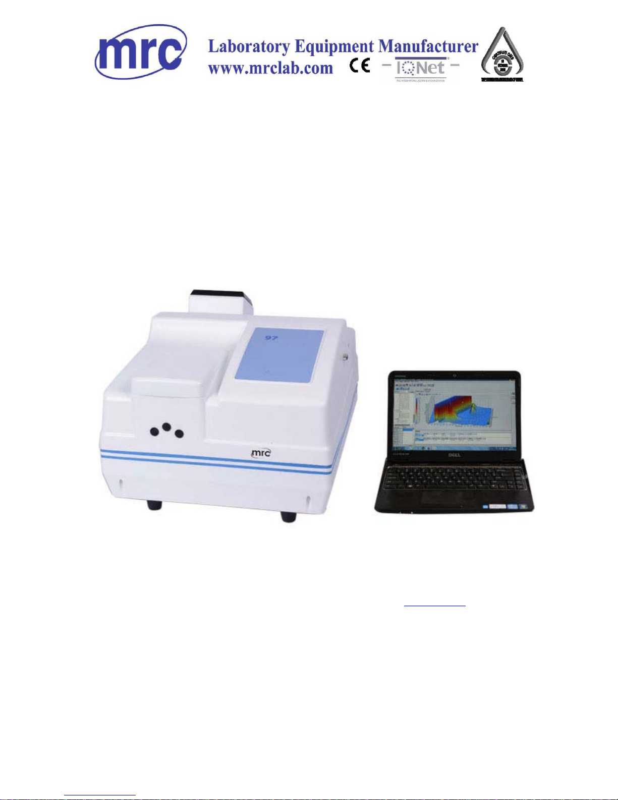
Fluorescent Spectrophotometers

SPECTRO-97 SERIES

Operation Manual

PLEAS

E READ THIS MANUAL CAREFULLY BEFORE OPERATION

Hagavish st. Israel 58817

Tel: 972 3 5595252, Fax: 972 3 5594529 mrc@mrclab.com

MRC.4.18

Preface

Thank you for purchasing the Fluorospectrophotometer of MRC Ltd. Please read this manual carefully before installation or first time using SPECTRO-97 series Fluorospectrophotometer. Fluorometry i

s a high sensitive, high selective and modern analysis method. Fluorometry provides excitation spectrum, emission spectrum, including luminous intensity, luminous life, fluorescence polarization and other information. It’s linear range of working curve is wide enough to become an important analysis method in Measure analysis. For proper use of SPECTRO-97 series Fluorospectrophtometer, basic knowledge of optical instruments and Molecular Fluorometry is needed. Computer operation skills are needed as well.

SPECTRO-97 series includes SPECTRO-97, SPECTRO-97 Pro and SPECTRO-97XP 3 kinds of

Fluorospectrophtometers. For more detail of parameter differences, please check manual chap.

1.4.

SPECTRO-97 series Fluorospectrophtometer

is a dual-monochromator fluorospec

trophtometer with fluorescence excitation wavelength scan, emission wavelength scan, 3D scan, Synchronous scan, time scan, quantitative analysis and other functions. The Fluorospectrophtometer should be operated with computer. This manual includes instrument instruction, software instruction and appendix. Chap. 6.3.5 is a value-added part. If you need this part, please contact us.

Special Statement

Pleas

e read this manual carefully before installation or operation. The company will not take responsible for any trouble or damage due to unproper use. The company has the final interpretation of this manual. Modifications of the manual due to improvements of the instrument will not be announced. The company will conduct 12 months free repair from the date of delivery if the instrument is in strict accordance withthe instructions and the transport safety specification. (Vulnerability and consumable parts are not included) Please useouroriginal packaging when returning the instrumentfor service with accessories and the warranty card. This manual is for SPECTRO-97series Fluorospectrophtometer. The company will post updates of all the information on our website.

Check out our website for more information. For more service, please dial our marketing department 972-3-5595252, or fax 972-3-5594529. Any chapter or images of this manual are not allowed to borrow, copy and translate to other languages without permission of the company.

Safety Signs

This sign indicates important part of the

instrument. Please follow instructions.

Please read and operate according to

the instructions following.

This sign indicates possible electric

harm.

Required by a professionally

qualified personnel according to the

appropriate procedures. (This label is

attached on the power switch and

trigger.)

This sign indicates heat o

n surface.

Precautions

1. The instrument is suitable for analysis in laboratory. If

the instrument is needed outside the lab, please make the field work environment meets the environmental requirements of the laboratory.

2. Please use our original packaging when moving

the

instrument.

Please boot the instrument in sequence. First, t

urn

the Xenon lamp power supply. Then turn on the main power. When shutting down, turn off the main power first, then turn off the Xenon lamp power supply. There will be 30 min before Xenon lamp becomes steady. Please wait 60 sec to retrigger the Xenon lamp if the Xenon lamp power shut down.

4. If the Xenon lamp power is not triggered and making noise, shut down the Xenon lamp power immediately and retrigger after 60 sec. Due to the fact that Xenon lamp life is closely related to the switching times, please minimize unnecessary Xenon lamp trigger times.

5. When the instrument is on, the temperature of th

vents

on top left corner is high. Please keep the air circulating and away from the vents surface. DO NOT observed Xenon light directly with naked eye.

6. Please make sure the fans on the left side and t

left

corner operate normally. If the fans are not functioning, please turn off the instrument for repairs.

7. As to protect PMT, DO NOT let light into the

sample

cell

when the gain is higher than 6. When using unknown sample in the test, set the gain from low to high gradually from 1 to 17.

8. Please check the Fluorescent zero and adjust

zero

after setting gain.

When an error occurred by wrong operation or o

ther

machine or instrument error, shut down the instrument immediately. When the software is not operating properly, Start Task Manager to end the "NeoLG.exe" process, then restart the software and the instrument.

10. DO NOT loose the screws in the monochromator. Keep the environment clean.

11.Cut the power before opening the instrument. Pay attention to the high-voltage electrical components on the left rear of the instrument.

12. Cover the instrument with dustproof if

the

instrument is not used for a long time.

Preface ............................................................................................................................................... 1

Special Statement .............................................................................................................................. 2

Safety Signs ...................................................................................................................................... 3

Precautions ........................................................................................................................................ 4

PART I：U s e r ’ s G u i d e ........................................................................ 9

1 Appearance & Performance ......................................................................................................... 10

1.1 Appearance ........................................................................................................................ 10

1.1.1 Body ....................................................................................................................... 10

1.1.2 Interface ................................................................................................................. 11

1.1.3 Power & Switches .................................................................................................. 12

1.1.4 Sample Compartment ............................................................................................. 13

1.2 Mode of Operation ............................................................................................................ 14

1.2.1 Signal Processing & Control System ..................................................................... 14

1.2.2 Light Path ............................................................................................................... 15

1.3 Functions ........................................................................................................................... 15

1.3.1 Modes For Measurement ........................................................................................ 16

1.3.2 Self Tests & Adjustments ....................................................................................... 16

1.4Performance ....................................................................................................................... 16

2 Booting & Shutting Down ........................................................................................................... 18

2.1 Booting Status ................................................................................................................... 18

2.1.1 Booting ................................................................................................................... 18

2.1.2 Fans Condition ....................................................................................................... 18

2.1.3 Multi-instruments Booting ..................................................................................... 19

2.1.4 Initialization ........................................................................................................... 19

2.2 Power Off .......................................................................................................................... 19

3 Installation .................................................................................................................................... 20

3.1Environment ....................................................................................................................... 20

3.1.1 Laboratory Environment ........................................................................................ 20

3.1.2 Work Bench ............................................................................................................ 20

3.1.3 Power ..................................................................................................................... 20

3.1.4Environment Change ............................................................................................... 20

3.2 Package ............................................................................................................................. 20

3.2.1 Check the Package ................................................................................................. 20

3.2.2 Unpack ................................................................................................................... 20

3.3 Installation ......................................................................................................................... 22

3.3.1 Cleaning ................................................................................................................. 22

3.3.2 Check the Power Source ........................................................................................ 22

3.3.3 Plug In .................................................................................................................... 22

3.4 Testing ............................................................................................................................... 22

3.4.1 Signal to Noise Ratio Test ..............................

........................................................ 22

3.4.2

Wavelength Test ..................................................................................................... 23

4 Maintenance ................................................................................................................................. 24

4.1Routine maintenance .......................................................................................................... 24

4.2 Light Source Maintenance & Replacement ....................................................................... 24

4.2.1 Maintenance ........................................................................................................... 24

4.2.2 Light Source Replacement ..................................................................................... 24

Part II：Software Manual ............................................................................................................... 25

5 Software Installation .................................................................................................................... 26

5.1 Requirements .................................................................................................................... 26

5.1.1 Hardware Requirements ......................................................................................... 26

5.1.2 System Requirements ............................................................................................. 26

.2 Install SPECTRO-97 Software ......................................................................................... 26

6 How To Use The Software ........................................................................................................... 31

6.1 Before Use ......................................................................................................................... 31

6.1.1 Connect to PC ........................................................................................................ 31

6.1.2 Link Procedure ....................................................................................................... 31

6.2 Functions ........................................................................................................................... 32

6.2.1 Measurement Modes .............................................................................................. 32

6.2.2 Interface ................................................................................................................. 33

6.3Software Operation ............................................................................................................ 38

6.3.1 Wavelength Scan .................................................................................................... 38

6.3.2 Time Scan ............................................................................................................... 47

6.3.3 Quantitative Analysis ............................................................................................. 54

6.3.4 3D-Scan .................................................................................................................. 65

6.3.5 Synchronous Scan .................................................................................................. 75

6.3.6 MORE CONVENIENT OPERATING METHODS .............................................. 83

PART III：APPENDIX .................................................................................................................. 95

Appendix I: Fluorescence & Phosphorescence ....................................................................... 96

F1.1 Theory ..................................................................................................................... 96

F1.2 Fluorescence analysis .............................................................................................. 99

Appendix II： MEASUREMENT OF INSTRUMENTAL RESPONSE ............................ 100

F2.1 Theory ................................................................................................................... 100

F2.2 Measurement of Instrumental Response on Excitation Side ................................. 100

F2.3 Measurement of Instrumental Response on Emission Side .................................. 102

Appendix III： Raman Scattering of Water & Detection Limit of Quinine Sulfate ............ 103

F3.1 Raman Scattering of Water ................................................................................... 103

F3.2 Water Raman Scattering S/N Ratio ...................................................................... 103

F3.3 Detection Limit of Quinine Sulfate ....................................................................... 104

Appendix IV： Quantitative analysis wavelength method .................................................. 105

F4.1 Single Wavelength ................................................................................................ 105

F4.2 Double Wavelengths ............................................................................................. 105

F4.3 Triple Wavelengths................................................................................................ 106

Appendix V： DETAILS ON QUANTITATIVE ............................................................... 107

F5.1 Linear Working Curve (1st order) ........................................................................ 107

F5.2 Quadratic Working Curve (2nd order) .................................................................. 107

F5.3 The correlation coefficient .................................................................................... 108

Appendix VI： Synchronous Scan ...................................................................................... 109

F6.1 Constant Wavelength Difference .......................................................................... 109

F6.2 Constant Energy Difference .................................................................................. 109

Appendix VII： Derivative Operation on Spectrum............................................................ 110

Appendix VIII： Smoothing ................................................................................................ 112

F8.1 Savitzky–Golay ..................................................................................................... 112

F8.2 Mean ..................................................................................................................... 112

F8.3 Median .................................................................................................................. 1 1 2

Appendix IX： Phosphorescence ........................................................................................ 113

F9.1 Theory ................................................................................................................... 113

F9.2 Phosphorescence Wavelength Scan ...................................................................... 113

F9.3 Phosphorescence Time Scan ................................................................................. 114

F9.4 Applications .......................................................................................................... 114

Appendix X： Chemiluminescence ..................................................................................... 115

Appendix XI： Multiple Excitation Scattering ................................................................... 116

Appendix XII： Accessories ............................................................................................... 117

PART I：User’s

Guide

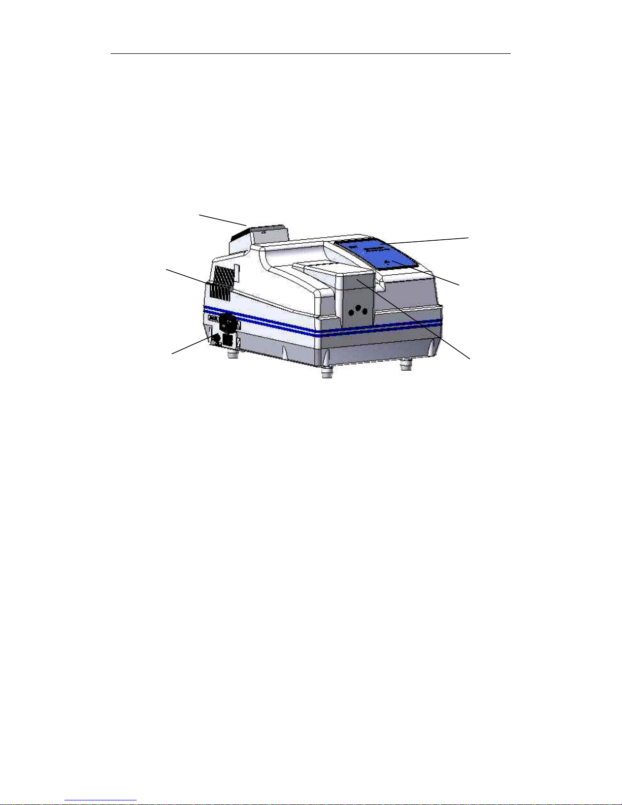
1 Appearance & Performance

1.1 Appearance

1.1.1 Body

Top Air-vent

Left Air-vent

Power Switch

Sample Compartment

Cover

Pilot Light

Panel

Fig.1-1 Body

Top Air-vent：Vent above the xenom light for air circulating. Please don’t touch. Left Air-vent：Vent beside the xenom light for air circulating. Power Switch：Please turn to chap. 1.1.3 for more information. Sample Compartment Cover：The cover can be opened up to less than 90 degrees. Pilot Light：Power light.

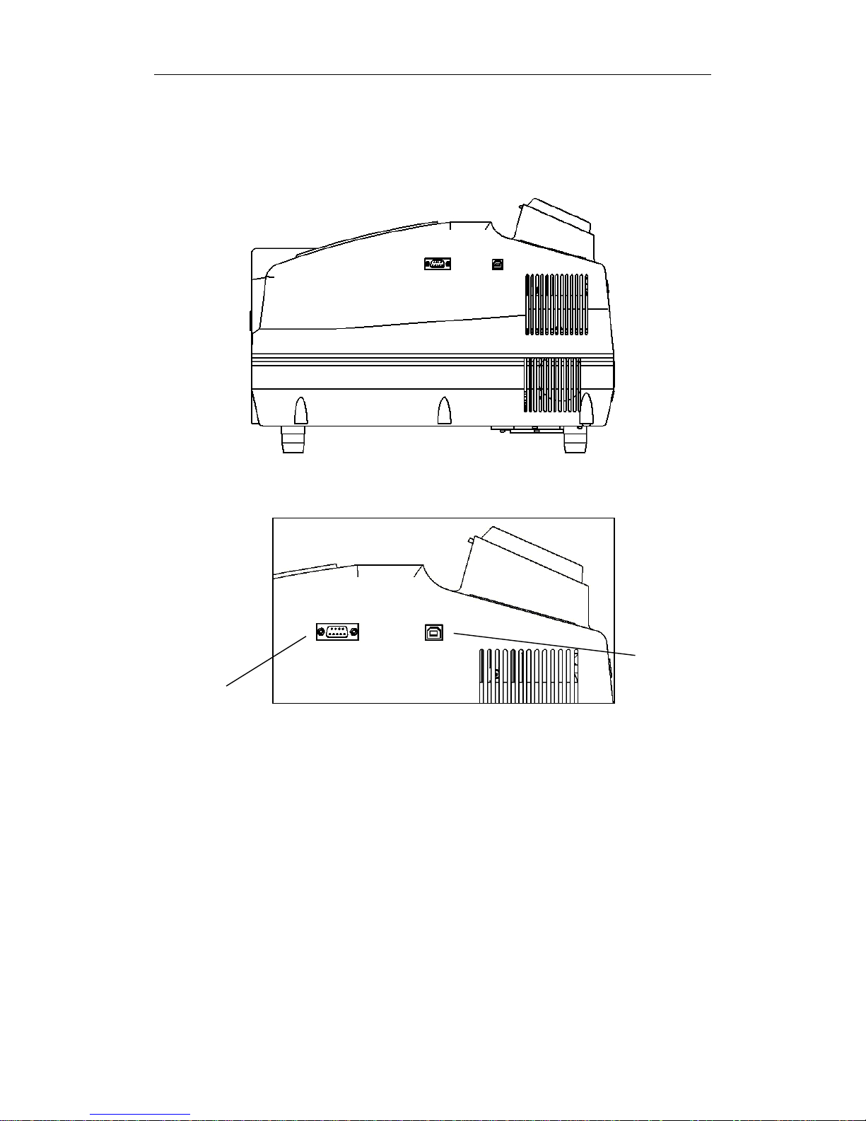
1.1.2 Interface

Fig.1-2 Side

View

Fig.1-3 Interface

RS232 Serial

Port

USB Port

USB Port：Link to PC with a USB cable. RS232 Serial Port：For debugging.

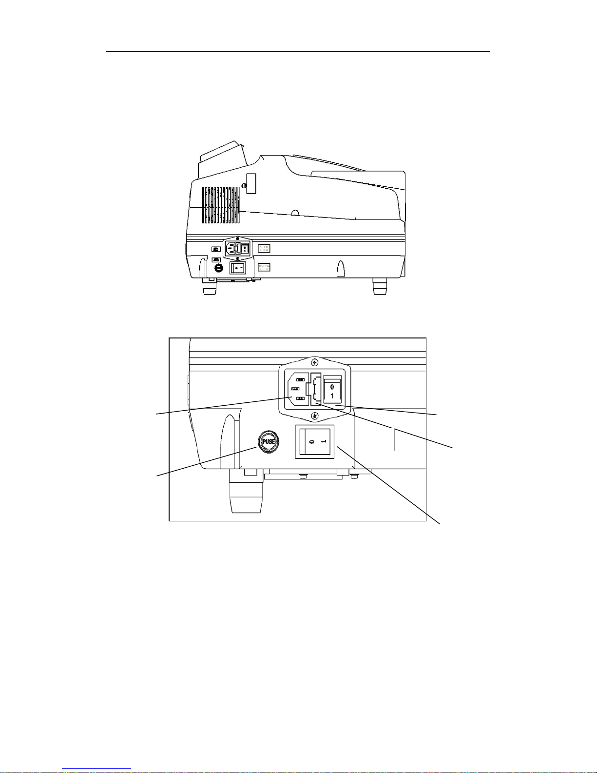
1.1.3 Power & Switches

Fig.1-4 Side

View

Fig.1-5 Power & Switches

Power

Plug-in

Xenom

Light

Main Power

Switch

Main Power

Fuse

Xenom Light

Switch

Power Plug-in：For connecting power cable. Xenom Light Fuse：For xenom light fuse. Xenom Light Switch：Turn on/off the xenom light. Main Power Fuse：For main power fuse. Main Power Switch：Turn on/off the instrument.

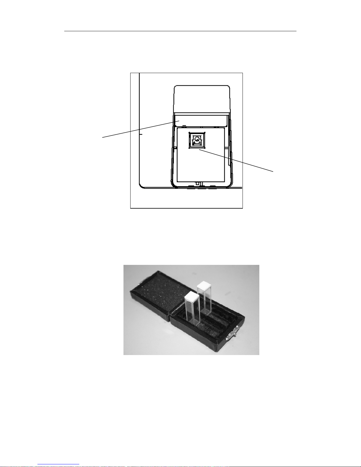
1.1.4 Sample Compartment

图 1-4F97XP 荧光分光光度计主机侧图

Fig.1-6 Sample Compartment

Compartment

Cover

Sample

Hold

Fig.1-7 Quartz Fluorescence Sample Pool

Sample Compartment：Sample hold inside. Sample Hold：For fixing sample pool.

1.2 Mode of Operation

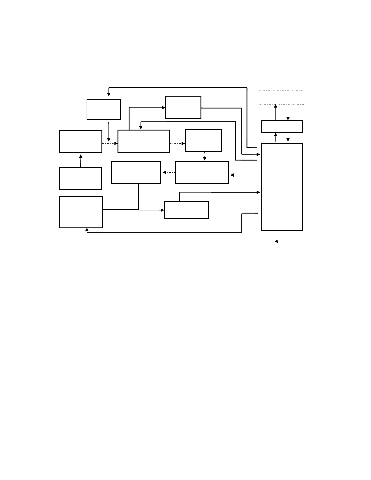
1.2.1 Signal Processing & Control System

Fig.1-8 Signal Processing & Control System

Controlled

Wavelengt

Xenon Light

Excitation

monochromator

Sample

Emission

monochromator

Photomultiplier

Pre-amplifier

Processor

USB

Negative

High

Voltage

Xenon Light

Power

Excitation

Monitor

Opitcal

Gate

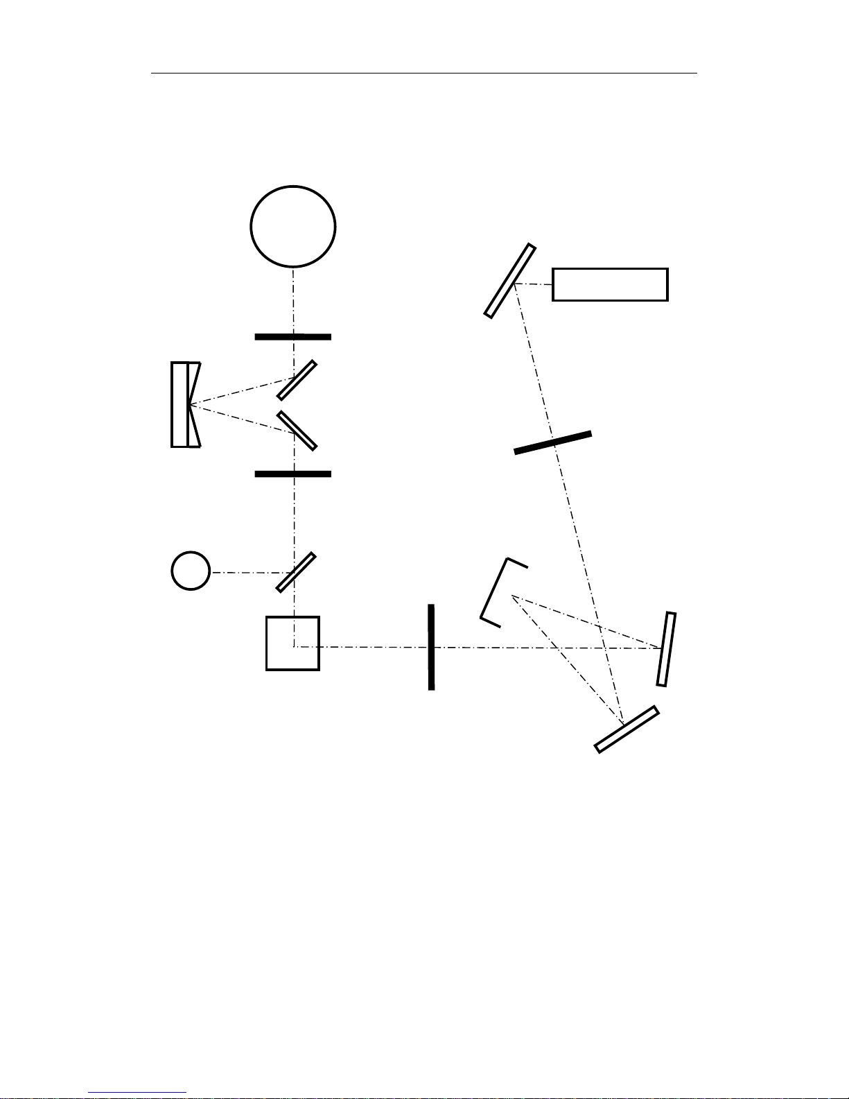
1.2.2 Light Path

Fig.1-9 Light Path

Lens

Len

Aspherical Mirror

Slit

Gratin

Sampl

Mirror2

Slit

Transflective

Mirror

Mirror3

Mirror4

Concav

Slit

Photomultiplier

Xenon

Light

Photocell

1.3 Functions

1.3.1 Modes For Measurement

1. Wavelength scan. Excitation wavelength scan provides spectrums of

fluorescence intensity which changes along with excitation wavelength under

fixed emission wavelength. Emission wavelength scan provides spectrums of

fluorescence intensity which changes along with emission wavelength under

fixed excitation wavelength.

2. Time scan. Time scan provides spectrums which changes along with time under

fixed emission wavelength and excitation wavelength.

3. Quantitative Analysis. According to the fluorescent spectra photometry, the

fluorescence intensity(F) is proportional to the concentration of the test sample(C)

under given conditions (the test group is dilute solution). Use fluorescent power F

and known sample concentration C to get standard curve. Then measure the

fluorescence of unknown sample to get the sample concentration.

4. 3D Scan. 3D scan includes excitation wavelength, emission wavelength and

fluorescence information.

5. Synchronous scan. The excitation side and the emission side scan at the same

time.

1.3.2 Self Tests & Adjustments

1. Self Tests & Adjustments

The instrument will initialize and self test while booting, including connection

detection, database detection, AD module detection, signal gain detection,

motion parts detection etc. Test result will be displayed on the screen and easy

for users to find problems.

1.4Performance

Tab.1-1 Performance of SPECTRO-97 series

Item Content

Excitation Source

150W xenon lamp（Hamamatsu）

Excitation

Wavelength

200nm~900nm

Emission Wavelength 200nm~900nm

Excitation Slit

SPECTRO-97XP/SPECTRO-97Pro：2nm、5nm、10nm、20nm

SPECTRO-97：10nm

Emission Slit

SPECTRO-97XP/SPECTRO-97Pro：2nm、5nm、10nm、20nm

SPECTRO-97：10nm

Wavelength Accuracy

SPECTRO-97XP：±0.4nm

SPECTRO-97/Pro SPECTRO-97：±1.0nm

Wavelength

Repeatability

SPECTRO-97XP：≤0.2nm

SPECTRO-97/SPECTRO-97Pro：≤0.5nm

Signal-to-Noise Ratio

SPECTRO-97XP:Raman peak of water(P-P):S/N≥200(10nm Slit）

SPECTRO-97/97Pro:Raman peak of water(P-P):S/N≥150(

10nm Slit）

Limit

SPECTRO-97XP：≤5×10

-11

g/ml（Quinine Sulfate Solution）

SPECTRO-97/97Pro：≤1×10

-10

g/ml（Quinine Sulfate Solution）

Linearity γ≥0.995

Peak Repeatability ≤1.5%

Stability(10min)

Zero Drift：±0.3

Value Limit：±1.5%

Wavelength Scan

Speed

Multi-speed Level, Maximum at 48000nm/min

Photometric

Quantity Range

0.00-10000.00

Data Transportation USB2.0

Power 200W

Power Source

AC 220V/50Hz； 110V/60Hz

Demension

380×445×310（mm）

Weight

Net Weight：12kg Gross Weight：14kg

2 Booting & Shutting Down

2.1 Booting Status

2.1.1 Booting

Put the instrument on steady platform. Make sure the main power and light power

switch are off(switch on 0). Plug in the power line.

There is a certain probability that the high voltage trigger of the Xenon light power

will affect other electrical equipment around. We highly recommend you check the

following status before turning on the Xenon light power:

1） Unplug the USB cable connecting PC and the instrument. 2） Make sure the grounding of power source is reliable. 3） If other instruments in the same platform were affected by the high trigger

voltage before, please shut down those instruments and turn on after the xenon

light is triggered.

4） Turn on the xenon light power, then turn on main power after the xenon light is

triggered.

Connect PC and the instrument with the USB cable, then run the PC software.

ATTENTION：

①If the xenon light is not triggered properly and making high noise,

shut down the xenon light power immediately. Please turn on the xenon

light after a few seconds.(It happens only when the power is not stable

or the xenon light is reaching its limit)

②As xenon lamp life and the switching times are closely related,

Please reduce unnecessary trigger.

③Xenon light needs 30 minutes to stable.

④Don’t turn on Xenon light without turning on the main power after.

2.1.2 Fans Condition

Please make sure the fans on the left side and on the top left are functioning every

time startup. If the fans are not working, shut it down and check.

！

2.1.3 Multi-instruments Booting

When using multiple instruments, please turn on all the xenon lights first, then turn

on all the main power to reduce the influence of the high trigger voltage.

2.1.4 Initialization

Initialization status will be displayed on computer software as Fig.1.3.2-1.

2.2 Power Off

When connecting to PC, close the software first; then turn off the main power; at

last turn off the xenon light power.

ATTENTION: To restart the Xenon light power, please wait for 60

seconds after power off.

！

3 Installation

3.1Environment

The instrument is suitable for analysis in laboratory environment. For its work with

computers, so need to meet the following working condition.

3.1.1 Laboratory Environment

Temperature 10～30 ℃, humidity under 85%. Avoid corrosive gas and the organic

and inorganic gases which are absorptive within the range of ultraviolet.

3.1.2 Work Bench

The work bench should be smooth and solid. Avoid vibration, dust, direct sunlight.

3.1.3 Power

AC 220V±22V，50Hz±1Hz or 110V±11V，60Hz±1Hz.

3.1.4Environment Change

If the instrument is needed in the field, please make sure the environment meets the

requirements above. Please use the original package moving instrument. If there are

special requirements please inform us when ordering.

3.2 Package

The instrument adopts carton packaging. Long-distance transport may require

additional outside wooden box.

3.2.1 Check the Package

Before unpacking, make sure the packaging is intact. If the package is damaged,

please contact with the transportation insurance.

3.2.2 Unpack

Open the case and carefully take out the instrument (Please keep the package for

transportation). Make sure the instrument and all accessories are correct according to

the package list. Please contact us if there is any mistake.

Table.3-1 Fluorescence spectrophotometer package list

Standard

fittings

SPECTRO-97 series instrument One piece

Fluorescence spectrophotometer

software

One set

Power Cable One piece

USB Cable One piece

Quartz fluorescence cell 10mm One piece

Fuse（2A/5A） two pieces

Instruction Manual for SPECTRO-97

series

Fluorospectrophotometer

One copy

Applications References Manual

One copy

Certification of products One copy

Packing list One copy

Guarantee repair list One copy

Dust proof One piece

Optional

spare

parts

Quartz fluore

scence cell 10mm

Glass fluorescence cell 10mm

Fuse（2A/5A）

USB cable

Power cable

Optional

accesso

ries

Cut-of

f filter

Membrane kind sample accessories

Powder kind sample accessories

Micro scale capillary sample accessories

Jacket sample pool accessories

200μL centrifuge tube accessories

Note: Optional spare parts and accessories will be delivered according to your

shipping contract.

3.3 Installation

3.3.1 Cleaning

Remove the tape and clean the surface.

3.3.2 Check the Power Source

Make sure the instrument power supply voltage and area voltage are correct.

3.3.3 Plug In

Put the instrument on a stable work table about 10 cm away from wall. Plug in the

power cable to the lab power.

3.4 Testing

3.4.1 Signal to Noise Ratio Test

1. Turn on the instrument and preheat. Light source and electronic components require to reach heat balance after startup.

Start operation after 30 minutes preheating.

2. Put in sample Choose a clean quartz fluorescence cell. Fill the quartz fluorescence cell with sample

(double distilled water). Then put it in the sample cell.

ATTENTION: Dirty quartz fluorescence cell will affect the accuracy

of the test.

3. Run emission wavelength scan

Choose “Wavelength Scan” –“Emission wavelength scan”. Set the excitation wavelength at 350nm, the emission wavelength at 300nm to 500nm. Set slit to 10nm. Set scan speed at 60nm/min. Response: auto. Gain: high. Run wavelength scan, then check the peak around emission wavelength 397nm. This peak is signal S.

4. Run time scan.

Choose “Time scan”. Set the excitation wavelength at 350nm. Set the emission wavelength at 397nm. Scan time 120 seconds. Slit 10nm. Response time 2 seconds. When the signal is stable(Let doubly distilled water expose more than three minutes above conditions), run time scan.

5. Calculate

Note the peak signal S and the Peak-valley value N. S/N is the Raman signal to noise ratio.

！

Attention：

①The energy of Raman is weak, so the measurement is easy to be

interfered. If the result looks bad, please test again.

②In order to protect the PMT tube, when the gain is high(above 6), please

don’t put high energy light source into the sample cell.

③Setting the gain will affect the fluorescent zero. Please reset zero after

changing gain.

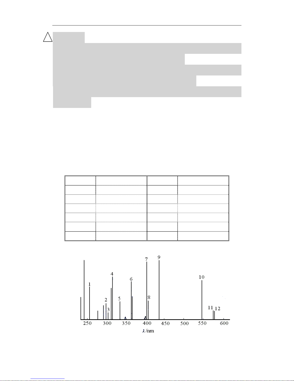
3.4.2 Wavelength Test

 The instrument will automatically adjust wavelength. If there is any wavelength mistake,

trained professionals are allowed to test wavelength with mercury-arc lamp or

fluorescent lamp. Learn the test method through training.

Mercury-arc lamp spectral line wavelength and figure below.

Table.3-2Emission spectra of low pressure mercury lamp in UV and visible region

NO. Wavelength/nm NO. Wavelength/nm

1 253.65 7 404.66

2 296.73 8 407.78

3 302.15 9 435.84

4 313.16 10 546.07

5 334.15 11 576.96

6 365.01 12 579.07

Fig.3-1Spectra of mercury-arc lamp

！

Power

4 Maintenance

4.1Routine maintenance

1. Always check whether it meets the requirements of the work environment in daily use.

2. Keep the vents functioning while the instrument is on.

ATTENTION: High temperature vents. Keep distance.

3. Keep the instrument clean. Add a dust cover when not in use. Use water to clean the instrument appearance. DO NOT use alcohol, ether, acetone and other organic solvents. Do not clean when the instrument is working.

4. Keep the quartz fluorescence cell clean.

4.2 Light Source Maintenance & Replacement

4.2.1 Maintenance

1. Keep the light source clean.

2. Strictly in accordance with the order of operations when turn on/off xenon light.

ATTENTION: When power on, turn on the xenon light power first,

then the main power. When power off, turn off the main power first, then

the xenon light power.

3. Xenon light will be hard to trigger when the power is not stable or the xenon

light is reaching its limit.

ATTENTION: If the xenon light is not triggered properly and making

high noise, shut down the xenon light power immediately. Please turn on

the xenon light after a few seconds.

4. Avoid repeated triggering xenon lamp.

As xenon lamp life and the switching times are closely related,

Please reduce unnecessary trigger.

5. Make sure that the instrument cooling fan is working properly. Make sure the

surface of the instrument top vents maintain good ventilation.

4.2.2 Light Source Replacement

Professionals are allowed to replace the light source. Specific methods and

calibration procedures will be introduced through training.

！

Part II：Software

Manual

5 Software Installation

Before reading this section, please read Part I carefully. Windows

XP system is recommended.

In order to run the software properly in Windows 7, please run the

．．．．．．．．．．．．．．．．．．．．．．．．．．．．．．．．．．．．．．．．．．．．．．．．．．．．．．

software in administrator account.

．．．．．．．．．．．．．．．．．．．．．．．．．．．．．．．

5.1 Requirements

5.1.1 Hardware Requirements

Hardware Minimum requirements

CPU Intel P4 2.0GHz or same level CPU

Memories 512M

Hard disk No less than 200M disk space

USB USB2.0

CD drive CD-ROM

Monitor resolution 1024*768

16-bit color

Table.5-1 Hardware requirements

5.1.2 System Requirements

Windows XP or higher version is recommended. Please turn off the screen saver

and

power management program while SPECTRO-97 Fluorescence Spectrophotometer

data processing software is running.

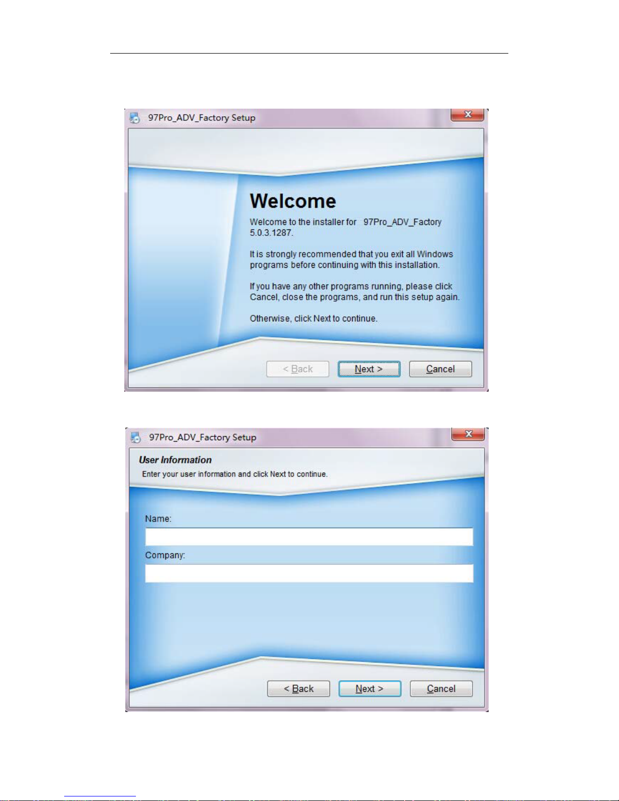
5.2 Install SPECTRO-97 Software

Put the software CD into the drive, the application will automatically start.

If the installation does not start, open X:\SETUP.EXE(X is the CD drive)

as Fig.5-1.This manual is based on SPECTRO-97 Pro.

Fig.5-1 Installation

Click “Next” in Fig.5-1, input user name and company name.

Fig.5-2 Information

Click “Next” in Fig.5-2 to set install path. Default path is as in Fig.5-3: C:\Program

File\MRC\SPECTRO-97Pro Fluorescence spectrophotometer. Click “Change”

to change the path. Click “Back” to go back, click “Cancel” to cancel.

Fig.5-3 Install path

Click “Next” to set account limit and shortcut path in fig.5-4.

Fig.5-4 Shortcut path & account limit

Fig.5-5 Installation information

Click “Next” if all the information is correct to start installation.

Fig.5-6 Installing

Wait for the installation. When the installation is complete, a notice will pop out as

fig.5-7. Then it is time to connect the instrument.

Fig.5-7 Installation complete

ATTENTION: CD serial number should be the same as the serial

number of the instrument. Otherwise, the software does not work

properly.

6 How to Use the Software

6.1 Before Use

6.1.1 Connect to PC

The instrument connects to the computer via USB cable, the computer will

automatically install the driver the first time connected, and please run software after the

driver is successfully installed.

6.1.2 Link Procedure

1. Link via USB cable

Connect the instrument to PC with USB cable. Start the PC.

2. Turn on the instrument

First turn on the xenon light power, then turn on main power when the xenon light is

lit. The instrument will enter online mode.

3. Initialization

Run SPECTRO-97 software. The s

oftware will start initializing and self tests.

Please turn to 1.3.2 for details.

4. Work mode

Click the very first button pointed out in red on tool bar in fig.6-1 to create a new

measurement. Choose a work mode in “Wavelength Scan”, “Time Scan”, “Quantitative

Analysis”, “3D Scan” and “Synchronous Scan”.

5. Power Off

Close the software, and then shut down main power and xenon light power.

If you shut down main power first, there will be a communicate error

on the software. Use task manager to close the NeoLG.exe.

！

Fig.6-1 Tool bar

6.2 Functions

6.2.1 Measurement Modes

There are 5 measurement modes:

1. Wavelength Scan:

（1） Shows the excitation spectra of the sample. （2） Shows the emission spectra of the sample. （3） Phosphorescence wavelength scan is available. （4） Supports automatic repeat scan. （5） Supports data printout.

2. Time Scan:

（1） Shows the sample fluorescence spectra change with time. （2） Phosphor Kinetics scan is available. （3） Supports automatic repeat scan. （4） Supports spectrum data processing. （5） Supports data printout.

3. Quantitative:

（1） Supports single-wavelength, dual wavelength and three-wavelength

quantitative analysis.

（2） Supports 1 to 3 times curve fitting. （3） Data decimal can be changed. （4） Programmable optical gate control. （5） Supports data printout.

4. 3D Scan:

（1） Shows 3D spectrum of excitation wavelength, emission wavelength and

fluorescence data.

（2） Supports 3D view of the spectrum. （3） Supports cross-sectional view of the spectrum. （4） Supports 3D contour map of the spectrum. （5） Supports data printout.

Synchronous Scan:

（1） Shows synchronous fluorescence spectroscopy spectrum. （2） Supports automatic repeat scan. （3） Supports data printout.

Docu

ments

6.2.2 Interface

6.2.2.1 Interface Modules

Info.

Fig.6-2 Interface modules

Status

Spectrum Information

Tool bar

6.2.2.2 Modules & Functions

1. Menu & Tools

1) Provides instrument controls and settings.

2) Tool bar are shortcuts for common features.

2. Document Browser

Document Brower shows files saved in Wavelength Scan, Time Scan and

Quantitative Analysis mode. Double click to open a file.

Fig.6-5 Document Browser

1) To reset the file saving path, click menu “Settings”->“Instrument Settings”.

Set a new saving path in the pop out window as Fig.6-6.

Fig.6-6 Set file path

2) Double click a spectrum file will show the spectrum and refresh.

3) Right click a file to open, rename or delete.

Fig.6-3 Menu & Upper Tool bar

Fig.6-4 Right Tool bar

4) Way of sorted files can be changed.

Fig.6-7 File menu

3. Information Window

Information window shows current data and info of the instrument.Including current

fluorescence value, excitation wavelength, emission wavelength, excitation and emission

slit, gain, the response time and optical gate condition. Double click to modify instrument

parameters.

Fig.6-8 Information Window

Any changes made here will not affect the parameters in Method

Settings. Information window is usually for status check.

4. Spectrum Window

1) Shows spectrum information.

2) Use mouse to zoom in and out. Press the left mouse button, drag the mouse

from top left to bottom right to draw a square, then release the button.

Spectrum in that square will be zoomed in. Drag the mouse the opposite

way to zoom out.

3) Click “Peaks” to show the peaks in the spectrum.

5. Status Window

1) Status window shows the current status of the instrument.

！

6.2.2.3 Tool Bar

Icon

Function

New Measurement

Open Spectrum

Save Spectrum

Print Spectrum

Show/Hide Status

Show/Hide Spectrum Information

Activate 2D Window

Activate 3D Window

Activate Quantitative

Analysis Window

Back to original coordinate

Auto coordinate

Y-axis enlarge 2 times

-axis reduce 2 times

Get/Cancel A

xis Data

Zoom In/Out

Show/Hide P

eaks

Show/Hide

Grid

Start/Stop

Open/Close

Optical Gate

Set W

avelength

Run/Ca

ncel Zero Adj.

Spectrum Properties

Print Data

Peak Threshold Setting

Spectrum Smoothing

Spectrum derivation

Spectrums C

alculation

Spectrums C

omparison

Table.6-1 Tool Bar Icons

6.3 Software Operation

6.3.1 Wavelength Scan

Wavelength Scan Flow chart

Fig.6-9 Wavelength Scan Flow chart

Power On

Run Software

New Measurement

Online

Set Parameters

Start Scan

Input File Name

Scan Complete

Choose“Wavelength Scan”

Confirm Parameters

Confirm Scan

Print Data

6.3.1.1 New Measurement

Create a new measurement.

Select “Files”->“Create Method” or click to enter Create Method Window.

1. Measurement Summary:

Fig.6-10 Measurement Summary

1） Measure Mode: Choose “Wavelength Scan”. 2） Operator: Input operator’s name. 3） Instrument:

The model of the connected instrument is indicated.

4） Comment:

Enter a description or notes on measuring conditions.

2. Instrument:

Fig.6-11 Scan Settings

1） Scan Mode: Excitation & Emission.

A. In excitation mode, X axis is excitation wavelength, Y axis is fluorescence

value. The instrument will do an excitation wavelength scan under a fixed

emission wavelength.

B. In emission mode, X axis is emission wavelength, Y axis is fluorescence

value. The instrument will do an emission wavelength scan under a fixed

excitation wavelength.

2） Data Mode: Fluorescence and phosphorescence mode available.*

1) The instrument will do Fluorescence scan in Fluorescence mode.

2) The instrument will do phosphorescence scan in phosphorescence mode. A

phosphorescence excitation time input window will be activate before the scan.*

3） Phosphorescence excitation time: Set the excitation time in phosphorescence

mode.*

4） Emission wavelength, excitation start wavelength, excitation end wavelength

are available in excitation mode.

Emission Wavelength: Input emission wavelength(200nm-900nm).

Excitation Start Wavelength: Input excitation start wavelength (200nm-900nm).

Excitation End Wavelength: Input excitation end wavelength (200nm-900nm).

5） Excitation wavelength, emission start wavelength, emission end wavelength

are available in excitation mode.

Excitation Wavelength: Input excitation wavelength(200nm-900nm).

Emission Start Wavelength: Input emission start wavelength (200nm-900nm).

Emission End Wavelength: Input emission end wavelength (200nm-900nm).

6） Scan Speed: Choose scan speed. The faster the noise get higher. 7） Scan Interval: Shows data sampling interval according to the scan speed. 8） Delay:

After pressing the Measure button, measurement is started following

the delay time set here. It is used for temperature stabilization, etc. In repeat

measurement, it is the time until the start of the first measurement.

9）

Excitation Slit: Set excitation slit.(SPECTRO-97 is fixed to 10nm)

10） Emission Slit: Set emission slit.(SPECTRO-97 is fixed to 10nm) 11） Gain(PMT): Set gain level by changing the PMT negative high voltage. 12） More Gain: Enlarge the gain range.

There will be a negative high voltage value besides each gain. This value is for

reference only. There will be some deviation from the actual value.

13） Response： Set the signal’s response time. Usually automatically set. 14） Spectral Correction： The instrument will use the last correction result to adjust

the wavelength parameter to correct sample spectrum when the Spectral

Correction is selected.(Please turn to Appendix II for more detail)

15） Shutter: To control the excitation time or condition of the sample.

A. When Shutter is selected, the instrument will open optical gate only when it’s

scanning to excite sample. When the scan stops, the optical gate will

automatically close. This function is for samples which are not stable when excite

by light.

B. When Shutter is NOT selected, the optical gate will be open. Sample will

always be excite.

C. Shutter will be on in phosphorescence mode.*

16）

Replicates: Set the number of repeat measurements. The instrument will only

scan once when it’s 1.

17）

Cycle time: Set a repetition interval.

3. Monitor：

Fig.6-12 Data Display

1） Y Axis: Enter the max and min point of Y axis. The max point should be larger. 2） Auto Adjust Y Axis: Y axis will automatically set by spectrum data.

4. Processing：

Fig.6-13 Spectrum Processing

1）

Processing choices: A list of data processing (Savitsky-Golay smooth, Mean smooth, Median smooth, Derivative) is shown. Select a data processing item, and click the rightward pointing arrow key between the Processing choices and Processing steps display fields. Then, the selected method appears in the Processing steps field.

2）

Processing steps: The processing sequence is displayed. To delete a processing method, first select the method, and then click the leftward-pointing arrow key between the Processing choices and processing steps display fields. Then, the selected method disappears from the Processing steps field.

3） Parameters: Click the “+” in Methods Chosen box to modify the parameters.

Click “OK” to confirm.

4）

Peak Finding: Automatically find peaks by giving threshold when the scan is

complete.

5. Report：

Fig.6-14 Data Printout

1） Output: Print Report or Save as Microsoft（R）Excel file. 2）

Output options: Choose the printout data. Check the content in “Properties”

button on the left after the scan.

3） Add Data: When “Spectrum Data” is checked, you can choose data section to

printout. Set the start wavelength, end wavelength and interval in the pop out

window, then click OK. Click the “+”to see the data section.

Fig.6-15 Set data section

Fig.6-16 Data section

4）

Clear Data: Clear current data section.

5） Click “Defaults” to reset the settings to default.

6） Click “Open” to open a saved method. It’s a *.FMTD file. 7） Click “Save” to save current settings.

6.3.1.2 Run Wavelength Scan

Wavelength scan procedure: Standby->Ready->Start Wavelength Scan ->Move to

Excitation(Emission) Wavelength -> Standby.

1. F

ile Name

Click

button to start a measurement. Input a file name or use system time as

file name.

2. S

top Scan

Click

to stop the scan.

6.3.1.3 Spectrum

The instrument will do wavelength scan with all the parameters. Spectrum will be

displayed in the spectrum window. The spectrum file will be automatically saved in the file

browser window.

Click to see details of the spectrum.

Icons Function

Reset Original Coordinate.

Auto Adjust Coordinate.

Enlarge Y Axis 2 Times

Reduce

Y Axis 2 Times

Get/Cancel A

xis Data

Zoom In / Out

Show/Hide P

eaks

Show/Hide

Grid

Peak Finding Details

Start/Stop

Open/Close

Optical Gate

Set W

avelength

Run/Ca

ncel Zero Adj.

Spectrum Smoothing

Spectrum derivation

Spectrums C

alculation

Spectrums C

omparison

Table.6-2 Functions for Spectrums

6.3.1.4 Printout

Icon Functions

Spectrum Properties

Print Data

Table.6-3 Functions for Printout

6.3.2 Time Scan

Time Scan Flow Chart

Fig.6-18 Time Scan Flow Chart

Power On

Open software

Create a measurement

Initialization

Set Parameters

Start Scanning

Input file name

Scan Complete

Select “Time Scan”

Confirm Parameters

Printout

Confirm Scan

6.3.2.1 Create a Measurement

Click “Files”->“Create Measurement” or click to create a new measurement.

1. General:

Fig.6-19 General

1) Measurement: Choose “Time Scan”.

2) Operator: Input operator’s name.

Instrument: The model of the connected instrument is indicated.

4) Comment: Enter a description or notes on measuring conditions.

2. Instrument

Fig.6-20 Scan Settings

1) Scan Mode: Fluorescence and phosphorescence mode available*

A. The instrument will do Fluorescence scan in Fluorescence mode.

B. The instrument will do phosphorescence scan in phosphorescence mode. A

phosphorescence excitation time input window will be activate before the scan.*

2) Phosphorescence excitation time: Set the excitation time in phosphorescence

mode.*

3) Emission Wavelength: Input emission wavelength (200nm-900nm).

4) Excitation Wavelength: Input excitation wavelength (200nm-900nm).

5) Scan Interval: This is a fixed value as 0.1s (100ms).

Scan time: Set the scan time.

Delay: After pressing the Measure button, measurement is started following the delay time set here. It is used for temperature stabilization, etc. In repeat measurement, it is the time until the start of the first measurement.

8) Excitation Slit: Set excitation s

lit. (SPECTRO-97 is fixed to 10nm)

9) Emission Slit: Set emission slit. (SPECTRO-97 is fixed to 10nm)

10) Gain (PMT): Set gain level by changing the PMT negative high voltage.

11) More Gain: Enlarge the gain range. There will be a negative high voltage value

besides each gain. This value is for reference only. There will be some

deviation from the actual value.

12) Response: Set the signal’s response time from “0.1”,“0.5”,“1”,“2”,“4”.The shorter

time, the more noise.

13) Replicates:

Set the number of repeat measurements. The instrument will only

scan once when it’s 1.

14) Cycle time: It’s available when Replicates is more than 1.

Set a repetition

interval.

3. Monitor:

Fig.6-21 Data Display

1、 Y Axis: Input the min point and max point of Y axis. 2、 Auto Adjust Y Axis: Y axis will automatically set by spectrum data.

4. Processing：

Fig.6-22 Spectrum Processing

2）

appears in the Processing steps field.

3）

4） Parameters: Click the “+” in Methods Chosen box to modify the parameters.

Click “OK” to confirm.

5） Peak Finding: Automatically find peaks by giving threshold when the scan is

complete.

5. Report:

Fig.6-23 Data Printout

1、 Output: Print Data or Save as Microsoft（R）Excel file. 2、

Output options: Choose the printout data. Check the content in “Properties”

button on the left after the scan.

3、 Add Data: When “Spectrum Data” is checked, you can choose data section to

printout. Set the start wavelength, end wavelength and interval in the pop out

window, then click OK. Click the “+”to see the data section.

4、 Clear Data: Clear current data section. 5、 Click “Defaults” to reset the settings to default. 6、 Click “Open” to open a saved method. It’s a *.FMTD file. 7、 Click “Save” to save current settings.

6.3.2.2 Run Time Scan

Time scan procedure: Standby->Ready->Start Time Scan -> Standby.

1. S

ave File:

Click

to start scan.Input file name in the pop out window or use system time as

file name.

2. S

top Scan:

Click

to stop the scan.

6.3.2.3 Spectrum Processing

The instrument will do Time Scan with all the parameters. Spectrum will be displayed

in the spectrum window. The spectrum file will be automatically saved in the file browser

window.

Click to see details of the spectrum.

Icon Functions

Reset Original Coordinate.

Auto Adjust Coordinate.

Enlarge Y Axis 2 Times

Reduce

Y Axis 2 Times

Get/Cancel A

xis Data

Zoom In / Out

Show/Hide P

eaks

Show/Hide

Grid

Peak Finding Details

Start/Stop

Open/Close

Optical Gate

Set W

avelength

Run/Ca

ncel Zero Adj.

Spectrum Smoothing

Spectrum derivation

Spectrums C

alculation

Spectrums C

omparison

Table.6-4 Functions for Spectrum

6.3.2.4 Printout Data

Icon Functions

Spectrum Properties

Print Data

Table.6-5 Functions for Printout

6.3.3 Quantitative Analysis

Quantitative Analysis flow chart

Fig.6-24 Quantitative-Analysis Flow Chart

Power On

Open Software

Create a measurement

Initialization

Set Parameters

Get fluorescence

values of standard

sample

Build regression curve

Get unknown sample value

Choose Quanti-Analysis

Confirm Parameters

Printout Data

Complete

Input file name

6.3.3.1 Create a Measurement

Click “Files”->“Create Measurement” or click to create a new measurement.

1. General:

Fig.6-25 General

easurement: Choose “Time Scan”.

2) Operator: Input operator’s name.

Instrument: The model of the connected instrument is indicated.

4) Comment: Enter a description or notes on measuring conditions.

2. Quantitative analysis

Fig.6-26 Quantitative analysis

1、

QA Options:

Type: Select the method of creating a calibration curve. Wavelength

only.

B. Number of wavelengths: the number of wavelengths used in Quantitative

analysis. Available from 1 to 3.(Details in appendix 4)

C. Significant Figures: Set Significant figures of the calculated value. Available

from 2 to 6.

D. Conc. Unit: Set Conc. Unit.

2、 Equation Parameters: Set equation type or curve fitting equation parameters

A. Equation Type: Choose from “

1st order”, “2nd order” and “3rd order”.

B. Custom Parameters: Choose to input your own parameters A0,A1,A2,A3.

The equation will be ConcA0A1∗X



A2∗XA3∗X



.(Details in

Appendix 5)

Force curve through zero: By putting a check mark in this box, a

calibration curve is created so that its factor A

0 passes through “0”

automatically.

3. Instrument

Fig.6-27 Instrument

1) Data Mode: Fluorescence mode.

2) Wavelength Mode: “Fixed Excitation Wavelength” and “Fixed Emission

Wavelength”. The Wavelength 1, 2, 3 are related to the number of wavelengths

in tab “Quantitative Parameters”.

A. When the number of wavelengths is 1, it would be the same whether in

“Fixed Excitation Wavelength” or “Fixed Emission Wavelength” mode. B. When the number of wavelengths is 2, Wavelengths 1 & 2 are available. ①

If you choose “Fixed Excitation Wavelength”, then the Excitation Wavelength is

fixed. When the instrument is doing measurement, it will go to emission wavelength 1,then go to emission wavelength 2. ② If you choose “Fixed

Emission Wavelength”, then the Emission Wavelength is fixed. When the

instrument is doing measurement, it will go to excitation wavelength 1, and then

go to excitation wavelength 2. C. When the number of wavelengths is 3, Wavelength 1, 2 & 3 are available.①

If you choose “Fixed Excitation Wavelength”, then the Excitation Wavelength is

fixed. When the instrument is doing measurement, it will go from emission wavelength 1 to emission wavelength 3.② If you choose “Fixed Emission

Wavelength”, then the Emission Wavelength is fixed. When the instrument is

doing measurement, it will go from excitation wavelength 1 to excitation

wavelength 3.

ATTENTION: When the number of wavelengths is 3, the value of wavelength 1, 2,

3 should be increasing or decreasing.

3) Wavelength 1: Input Excitation Wavelength 1 and Emission Wavelength

1(200-900nm).

4) Wavelength 2: Input Excitation Wavelength 2 and Emission Wavelength

！

2(200-900nm).

5) Wavelength 3: Input Excitation Wavelength 3 and Emission Wavelength

3(200-900nm).

6) Pre-Excitation Time: The instrument allows light to illuminate the sample

pre-excitation time before measurement. During this time the instrument will not

do fluorescence measurement. The time of this part is to stabilize the excitation

light and the sample.

7) Integration time:

A function for obtaining data averaged over the specified

time for the purpose of acquiring stabilized data.

8) Excitation slit: Set excitation slit.(SPECTRO-97 is fixed to 10nm)

9) Emission slit: Set emission s

lit.(SPECTRO-97 is fixed to 10nm)

10) Gain (PMT): Set gain level by changing the PMT negative high voltage.

11) More Gain: Enlarge the gain range. There will be a negative high voltage value

besides each gain. This value is for reference only. There will be some deviation

from the actual value.

12) Response： Set the signal’s response time from “0.1”,“0.5”,“1”,“2”,“4”.The shorter

the more noise.

13) Shutter: To control the excitation time or condition of the sample.

A. When Shutter is selected, the instrument will only open the shutter when

measuring samples. The shutter will automatically close when the

measurement is complete. This function is for samples which are not stable

when excited by light.

B. When Shutter is NOT selected, the shutter will be open. Sample will always

be excited.

4. Standards

Fig.6-28 Standards

Sample table: Sample table gives a list of standards for sample measurement or calibration curve preparation. This table contains the items listed below.

2. Lines: Number of Standard Samples.

1) “Update”:

By clicking this button, sample numbers are set by the entered

number

of samples. The displayed sample names, comments, etc. are

all cleared.

2) “Insert”:

When the initial screen is opened, the Insert button becomes

active. Click this button t

o insert data at the end of the sample list.

“Delete”: Click the column of the sample No. to be deleted, and it becomes active. Now click the Delet

e button and the item is deleted.

5. Report

Fig.6-29 Report tab

Output: Print Data or Save as Microsoft（R）Excel file.

2. Output options: Choose the printout data. Check the content in “Properties”

button on the left after the scan.

3. Clear Data: Clear current data section.

4. Click “Defaults” to reset the settings to default.

5. Click “Open” to open a saved method. It’s a *.FMTD file.

6. Click “Save” to save current settings.

6.3.3.2 Quantitative-Analysis Interface

Click ”OK” in the last step to enter Quantitative-Analysis interface.

Fig.6-30 Quantitative-Analysis Interface

1. Menu, Toolbar, File Browser, Information and Status are the same as

Chap.6.2.2.2.

2. Property: Check all the parameters of Quantitative-Analysis.

ATTENTION: The parameters cannot be modified in the window.

Please create a new measurement to modify the parameters.

Fig.6-31 Propert

y Window

！

Menu & Toolbar Standard

Sample

Curve

Unknown Sample

Property

Status

File Browser

Information

6.3.3.3 Conducting Measurement

1. In the Standards window, you can modify sample name, description and

concentration; add or delete sample; check the fluorescence value of samples.

1) Modify sample name, description and concentration: Click “Edit”, then double

click in the table to modify the content you want. Then click “OK” to confirm.

2) Measure a fluorescence value: Click to select a sample in the table, then click

“Start” button. The instrument will start measurement. The Status Window will

goes as “Standby”->“Remaining time **sec”->“Standby”.

3) Add Sample: Click “Edit”, then click “Insert”. There will be another line in the

standards window. Click “OK” to finish.

4) Delete Sample: Click “Edit” and click a line you want to delete, then click

“Delete”. Click “OK” to finish.

5) Choose the sample data needed in curve calculation: Click “Edit”, then click the

check mark in “Calculate” row if you want to use this data for calculation.

ATTENTION: Pay attention to the Zero adjustment. Click to do

Zero adjustment, click again to reset the Zero point.

Click “Build Equation” to build the curve of standard sample when finishing

measurement as Fig.6-33. The abscissa is fluorescence value, the ordinate is

the concentration value. The equation is under the figure.(Check the

mathematical algorithms of the regression curve in Appendix V)

Fig.6-32 Standards Window

！

6.3.3.4 Measurement of the sample

When the regression curve is created, you can start measuring the sample. Operate

the test sample in samples window as Fig.6-34. There are functions in the sample

window: Measure, Modify, Delete and Clear.

1、 Change sample name & note: Click “Edit” button, then double click the frame

you want to modify. Click “OK” to confirm the modification and back to test

sample window.

2、 Measure sample fluorescence value & concentration value: Click a sample

fluorescence value or concentration value frame, then click “Measure” button to

measure the sample. The fluorescence value and concentration value of the

sample will be in “Fluorescence” and “Concentration” column. When measuring

sample, the Status window will show current status as “Standby”“Seconds

Counting: ** sec”“Standby”.

Fig.6-33 Regression Curve

Fig.6-34 Sample Window

3、 Delete sample: Click “Edit” button, then click the line you want to delete and

click “delete” button to delete the sample. Click “OK” to confirm the modification

and back to test sample window.

4、 Clear sample list: Click “Edit” button, then click “Clear” button. Click “OK” to

confirm the modification and back to test sample window.

6.3.3.5 Printout Data

Icon Function

iew spectrum information & choose printout content

and format.

Printout Data.

ab.6-6 Toolbar icon functions

6.3.4 3D-Scan

3D fluorescence spectrum has a characteristic of the "fingerprint". We can get all

kinds of information on the sample map through the analysis of three-dimensional

fluorescence spectrum, Including the excitation wavelength of Rayleigh scattering and

secondary scattering, Raman shift samples, the optimal excitation wavelength, the best

fluorescence peak wavelength.

3D Scan Procedure

Power On

Open Software

Create a method

Online Initialization

Set Parameters

Start Scan

Input Spectrum Name

Scan done

Choose“3D Scan”

Confirm Parameters

Confirm Scan

View 3D Spectrum

Printout Data

Fig.6-35 3D Scan Procedure

6.3.4.1 Create a method

First of all, create a method.

Click “File”“New Method” or click to enter the window below in Fig.6-36 to

create a method.

1. General:

Fig.6-36 General tab

1) Measure Mode: Choose “3D Scan”.

2) Operator: Input operator’s name.

Instrument: The model of the connected instrument is indicated.

4) Comment: Enter a description or notes on measuring conditions.

2. Instrument:

Fig.6-37 Instru

ment tab

1） Scan Mode: Fluorescence mode. 2） Excitation Start Wavelength: Input excitation wavelength (200nm-900nm). 3）

Excitation End Wavelength: Input excitation wavelength (200nm-900nm). 4） Excitation Sampling Interval：In the 3-dimensional measurement mode,

emission spectrum measurement is repeated while shifting the excitation

wavelength. Therefore, a shorter sampling interval on the excitation side will

result in a longer measurement time.

5） Emission Start Wavelength: Input emission wavelength (200nm-900nm). 6） Emission End Wavelength: Input emission wavelength (200nm-900nm). End

wavelength should be longer than start wavelength. 7） Scan Speed: Set scan speed. The faster the speed is, the shorter the scan

takes, and with more noise. 8） Scan Interval: set the interval of the data point in the spectra according to the

scan speed. 9） Excitation Slit: Set a slit width for the excitation side.(SPECTRO-97 is fixed in

10nm) 10） Emission Slit: Set a slit width for the emission side.(SPECTRO-97 is fixed in

10nm) 11） Gain (PMT): Set the voltage level of the photomultiplier tube to change the gain. 12） More Gain: More Gain levels to choose. 13） Corrected spectra: A function for determining the spectrum inherent to a

sample by correcting the photometer wavelength characteristic using the saved

instrument parameters, following measurement with the instrument parameters

for photometer control. When this setting is at ON, the instrument will use the last

correct result to correct the spectra. (Turn to Appendix for detail) The suitable

wavelength range of Rhodamine B solution for spectral calibration is

250nm-600nm. 14） Response Time: Set a response time. Set auto usually. 15） Shutter Control: The shutter can be automatically closed in other than

measurement for suppressing sample deterioration due to the energy of

excitation beam and opened when measurement starts. When you put a check

mark at the head, the shutter will close and open at start of measurement. The

shutter will close again when measuring wavelength begins returning to the

start wavelength after measurement in the wavelength scan mode.

16） Replicates: Set the repeat times of scans. 17） Cycle time: Set the waiting time between two scans.

3. Monitor：

Fig.6-38 Monitor Tab

1、 Y Axis: Input start point and end point of the Y Axis. 2、 Auto set Y Axis: Y axis will automatically set according to Y axis data.

4. Spectra Processing：

Fig.6-39 Processing Tab

1、 Available Methods: There are 4 methods of data processing."Polynomial

smooth", "smooth mean", "median Smooth" and "derivative" are available.

1) Select a method in “available” window, then press to move the

method to “selected” window.

2) Select a method in “selected” window, then press to move the

method to “available” window.

2、 Selected: the selected methods are in this window. When the scan is done, the

software will use selected methods to process scan data.

3、 Modify Parameters: Click the “+” in front of a method in Selected window to

show the parameters. Click to modify, then press OK to confirm.

4、 Peak Finding: Set the threshold and sensitivity to find peak after the scan.

5. Report：

Fig.6-40 Report Tab

1、 Output: Transfer data into Microsoft Excel format. 2、 Output Options: Put a check mark to select the output data.

6.3.4.2 Run Wavelength Scan

The status will be: “Standby” “Ready to scan” “Moving excitation wavelength”

“Moving emission wavelength” “Start wavelength scan” “Move emission wavelength”

“Standby”.

A. File Name

Click the start measurement button , there will be a popout window to input a file

name. Press OK to start 3D scan. Keep it blank if you want to use the current system time

as file name.

B. Scan Stop

Click to stop the scan.

6.3.4.3 3D Spectrum Processing

A. Spectrum Display

When the scan is running, spectrum data will be displayed in the spectrum window as

2D figure. The spectrum will be displayed in the spectrum window as 3D figure after

scan.The spectrum file will be automatically saved.

B. 3D Scan Toolbar

Icon Function

Click

to show the front view

Click to sho

w the rear view

Click

to show the left view

Click

to show the right view

Tab.6-7 3D Functions

3D window

Tool bar

Fig.6-41 3D Scan Interface

C. Spectrum Window

1. 3D Spectrum Tab: 3-D Scan data can be displayed in 3D view. The

spectrum is a composition of emission wavelength axis, the excitation

wavelength axis fluorescence value axis, contour and color notification.

Fig.6-42 3D Spectrum Tab

Click these tabs to show

3D view, Contour view and 3D contour view. Click buttons in tab 6-8 for more

functions.

Icon Function

Click

to zoom and move the spectrum. Left key

operations are the same as 6.2.2.2. Hold right key to

move the spectrum.

Click

to rotate the spectrum. Hold left key to rotate with

mouse moving. Hold right key to move the spectrum.

Click to move the spectrum.

Click

to zoom the spectrum. Hold left key and move the

mouse down to zoom out. Hold left key and move the

mouse up to zoom in. Hold right key to move the

Tabs

Buttons

spectrum.

Click

to change the depth. Hold left key and move the

mouse to adjust the depth of the spectrum. Hold right

key to move the spectrum.

Tab.6-8 Spectrum Controls

2. Contour Tab: Shows the contour line in 2D view as Fig.6-43.

Fig.6-43 Contour Tab

Contour tab includes contour wind

ow, emission window and excitation window.

（1） Contour lines: X axis is emission wavelength. Y axis is excitation

wavelength.

From these contour lines, excitation and emission spectra can be read out. As the cursor is moved, the cursor-specified excitation and emission spectra are displayed in side window.

（2） Excitation Spectrum:

An excitation spectrum at the cursor position in contour lines window is displayed. Wavelength and photometric value can be read in the window.

（3）

An emission spectrum at the cursor position in contour lines window is displayed. Wavelength and photometric value can be read in the window.

Contour lines

Emission spectrum

Excitation spectrum

3. 3D Contour Tab: Shows all the 2D spectrums in 3D view as Fig.6-44.

Fig.6-44 3D Contour Tab

6.3.4.4 Printout

Icon Function

Shows

the spectrum information. Select printout format

and content.

Click to printout data.

ab.6-9 Printout Functions

Tabs

Buttons

6.3.5 Synchronous Scan

Synchronous Scan flow chart

Fig.6-45 Synchronous Scan flow chart

Boot

Run software

Create a measurement

Initialization

Set parameters

Start scanning

Input file name

Scan complete

Choose Synchronous scan

Confirm parameters

Confirm file name

Printout

6.3.5.1 Create a measurement

Click “File”“Create measurement” or click icon to create a measurement.

A. General

Fig.6-46 General

1、 Measurement: Choose “Synchronous scan” 2、 Operator: Input operator name. 3、 Instrument: The model of the connected instrument. 4、 Comments: Enter a description or notes on measuring conditions.

B. Instrument

Fig.6-47 Instrument Tab

1、 Scan mode: Constant Wavelength Synchronous Fluorescence (CWSF) &

Constant Energy Synchronous Fluorescence (CESF). Constant Wavelength

Synchronous Fluorescence: Excitation and emission sides scan at the same

time in a fixed wavelength difference. Constant Energy Synchronous

Fluorescence: Excitation and emission sides scan at the same time in a fixed

energy difference.

2、 Data mode: Fluorescence mode 3、 Scan mode: If the scan mode is “WL Adaption”, “CWSF” is available. If the scan

mode is “Difference Adaption”, “Emission wavelength” is not available. Click

“Refresh” to see the emission wavelength.

1) If the scanning style is “WL Adaption”, emission wavelength is not available.

Edit excitation start wavelength or CWSF then click “Refresh”, emission

wavelength will be available.

2) If the scanning style is “Difference Adaption”, CWSF is not available. Edit

emission wavelength and excitation start wavelength then click “Refresh”, CWSF

will be available.

1、

This is the start wavelength for wavelength scan on the emission side.( 200

to 900 nm

)

2、

This is the start wavelength for wavelength scan on the excitation side.( 200

to 900 nm

)

3、

This is the end wavelength for wavelength scan on the excitation side. ( 200

to 900 nm

)

4、 Constant Wavelength Difference & Constant Energy Difference: Constant

wavelength difference is the difference between excitation start wavelength and

emission start wavelength. Constant energy difference is the difference

between energy of excitation start wavelength and emission start wavelength.

5、 Scan Speed:

Set a wavelength scan speed.

6、 Scan Interval: Shows data sampling interval according to the scan speed. 7、 Delay: After pressing the Measure button, measurement is started following

the delay time set here. It is used for temperature stabilization, etc.

8、 Excitation Slit：Select a slit width for the excitation side.（SPECTRO-97 is fixed to 10nm） 9、 Emission Slit：Select a slit width for the emission side.（SPECTRO-97 is fixed to 10nm） 10、 PMT Voltage: A function for controlling the voltage of the photomultiplier

tube. It will change the gain.

11、 More Gain: More gain level available. This negative high value is for reference only, and the actual negative high voltage value will have a bias. 12、 Response: Response time of wavelength scan. Select Auto usually. 13、 Corrected spectra: A function for determining the spectrum inherent to a

sample by correcting the photometer wavelength characteristic using the saved instrument parameters, following measurement with the instrument parameters for photometer control. Rhodamine B solution suitable for spectral calibration wavelength range is 250 to 600nm.

14、 Shutter control: The shutter can be automatically closed in other than

measurement for suppressing sample deterioration due to the energy of excitation beam and opened when measurement starts.

When you put a check mark at the head, the shutter will close and open

at start of measurement. The shutter will close again when measuring wavelength begins returning to the start wavelength after measurement in the wavelength scan mode.

2) If it’s not chosen, the shutter is open constantly.

15、

Replicates: Set the number of repeat measurements.

16、

Cycle time: Set a repetition interval.

C. Monitor

Fig.6-48 Monitor Tab

1、 Y Axis: Enter the start point and end point of Y axis. 2、 Auto Y Axis: Automatically adjust Y axis when a check mark on.

D. Processing

Fig.6-49 Processing Tab

1、

Processing choices: Used for obtaining an average spectrum in repeat measurement. A list of data processing (Savitsky-Golay, Mean smooth, Median smooth, Derivative) is shown.

Select a data processing item, and click the rightward-pointing arrow key

between

the Processing choices and Processing steps display fields .

Then, the selected method appears in the Processing steps field.

The processing sequence is displayed. To delete a processing method,

first

select the method, and then click the leftward-pointing arrow key

between the Processing choices and Processing steps display fields. Then, the selected method disappears from the Processing steps field.

2、

Processing steps:

3、 Change Parameters：

If you want to carry out any smoothing in Processing steps, click the + in front of the relevant item and the smoothing parameters can be changed.

4、

Peak Finding: Select a peak detection method indicated in the data processing window. Set a detection limit for the photometric value axis of peak and valley.

E. Report

Fig.6-50 Report Tab

1、

Output: Print Report and Use Microsoft® Excel are available.

2、

Output options: Check these items to add into printout report. Click to

check out the chosen items.

3、 Add Data: When “Spectrum Data” is checked, you can choose data section to

printout. Set the start wavelength, end wavelength and interval in the pop out

window, then click OK. Click the “+”to see the data section.

6.3.5.2 Run Synchronous Scan

There is a changing process running synchronous scan: “Standby”“Ready”“Start

wavelength scan”“Moving excitation and emission wavelength”“Standby”

一、 File Name

Click to enter a file name. Click OK to start the scan. Keep it blank to use the

current system time as file name.

二、 Stop Scan

Click to stop the scan.

6.3.5.3 Spectrum Processing

Spectrum will be displayed in the spectrum window. The spectrum file will be

automatically saved in the file browser window.

Click to see details of the spectrum.

Icon Functions

Reset Original Coordinate.

Auto Adjust Coordinate.

Enlarge Y Axis 2 Times

Reduce

Y Axis 2 Times

Get/Cancel A

xis Data

Zoom In / Out

Show/Hide P

eaks

Show/Hide

Grid

Peak Finding Details

Start/Stop

Open/Close

Optical Gate

Set W

avelength

Run/Ca

ncel Zero Adj.

Spectrum Smoothing

Spectrum derivation

Spectrums C

alculation

Spectrums C

omparison

Tab.6-10 Toolbar

6.3.5.4 Printout Data

Icon Functions

Spectrum Properties

Print Data

Tab.6-11 Toolbar

6.3.6 MORE CONVENIENT OPERATING METHODS

6.3.6.1

Arithmetic Operation between Spectra

Arithmetic Operation Procedures

Fig.6-51 Flowchart

Boot

Run software

Scan to get a spectrum

Initialization

Enter calculation interface

Choose spectrum type

Choose target

Choose calculate method

Calculate

Save & printout

Arithmetic Operation includes addition, subtraction, multiplication and division

among the same type of spectrum. Click on the right to enter the spectrum

compare window as Fig.6-52.

Fig.6-52Arithmetic Operation

Arithmetic Operation Interface:

Functions: Calculations and data processing as Tab.6-12

Buttons Function

Click

to choose Add, Minus, Plus and

Division

Click

to calculate

Click to save the spectru

Click to printout

Tab.6-12 Arithmetic Functions

2. Target spectrum 1 & Spectrum files section 1: Double click the spectrum

file in section 1, then the spectrum will be displayed in spectrum 1.

3. Target spectrum 2 & Spectrum files section 2: Double click the spectrum

file in section 2, then the spectrum will be displayed in spectrum 2.

4. Spectrum type: Click tag to change spectrum.

5. Result: Shows the result spectrum.

Result

Function Target spectrum

Target spectrum 2

Spectrum files 2

Spectrum type

Spectrum

files 1

Spectrum

type

6.3.6.2Overlaid Display of Spectra

Overlaid Display of Spectra

Fig.6-53 Flowchart

Boot

Run software

Scan to get spectrum

Initialization

Enter spectrum interface

Choose spectrum type

Choose target spectrum

Enter overlaid interface

View results

Save & Printout

This function is convenient for comparison of two or more spectra of the same type. Click

to enter the overlaid interface as in Fig.6-54.

Fig.6-54Overlaid Display Interface

Interface:

1. Type: Choose the spectrum type. Excitation spectrum, emission spectrum,

time scan spectrum and synchronization scan spectrum are available.

2. Files: Shows the spectrum files of the type above. Hold “Ctrl” to select

multiple spectrums.

CHOOSE NO MORE THAN 9 SPECTRUMS.

B. Click “OK” to enter interface as Fig.6-55.

Fig.6-55 Overlaid Viewer

The selected spectrums are in the overlaid viewer in different color.

2. Spectrum Select: Choose the spectrums to compare.

3. Functions: To save, print the spectrum. Click “Return” to go back Fig.6-55.

Click “Cancel” to exit overlaid.

！

Files

Typ e

Spectrum

Spectrum Select Function

6.3.6.3 Detection of Spectral Peaks

Detection of Spectral Peaks Procedure

Fig.6-56 Flowchart

The spectral peaks and valleys are detectable

automatically. Select the Find Peaks command from the Data

menu or click button, and a window as in Fig. 6-57

appears. Set threshold of Y axis and X axis. If the peak is

high, the Y axis threshold could be larger; if the peak is wide,

the X axis threshold could be larger.

Click / to show/hide information of the peak coordinates.

Boot

Run software

Scan to get spectrum

Initialization

Enter Peak finding

Set threshold

Show/Hide peak Coordinates

Save & Printout

Fig.6-57 Peaks

6.3.6.4 Smoothing of Spectrum

Smoothing of Spectrum Procedure

Fig.6-58 Flowchart

Smoothing is to reduce the noise of spectrum. Click

to set smoothing parameters in Fig.6-59. Select function type,

Smoothing order, Number of points and Number of times then

click “OK” to see the effect.

Boot

Run software

Scan to get spectrum

Initialization

Enter Smoothing

Set function type & parameters

View results

Save & printout

Fig.6-59 Smoothing

parameters

Type Smoothing order Number of points Number of times

Savitsky-Go

lay

The highest power

of the polynomial

Set the number of points

to be used in

calculation.(odd number)

Set the number of

smoothing operations.

Mean --------------- Set the number of points

to be used in calculation.

Set the number of

smoothing operations.

Median --------------- Set the number of points

to be used in calculation.

Set the number of

smoothing operations.

Tab.6-13 Smoothing Parameters

6.3.6.5 Derivative Operation on Spectrum

Derivative Operation Procedure

Fig.6-60 Flowchart

Derivative Operation on Spectrum is to enhance

the resolution of peaks. Derivation can distinguish

various disturbances affecting the shape of the

spectrum peaks. Usually combining the smoothing

operation.

Click to open Derivative parameters

window. Set Derivative order and click “OK” to see the

result.

Boot

Run software

Scan to get spectrum

Initialization

Derivative Operation

Set order

View result

Save & printout

Fig.6-61 Derivative parameters

6.3.6.6 Instrument Settings

This is to change the save path, file name and spectrum type. Click “Settings”

“Options” to open settings window in Fig.6-62.

A. General tab：

Fig.6-62 General tab

1. Default Method: Instrument use default parameters.

2. Specified method: Instrument uses specified parameters.

3. Default Directory: Instrument uses default path.

4. New Default Directory: Instrument uses specified path.

B. Storage Tab：Fig.6-63

Fig.6-63 Save Tab

1. Add Subhead when repeated scan: Automatically add a number suffix to file

names.

2. From: Set the start number.

3. Places: Set number digits.

4. Reset after rename: Auto reset number when using another name.

C. Spectrum Tab

Fig.6-64 Spectrum Tab (Curve & Coordinates)

Fig.6-65 Spectrum Tab (Background Setup)

1. Curve & Coordinates Tab: Sets color and width of curves, and color, width, height

and shape of dots.

1) Curve color: Sets curve color.

2) Serie width: Sets curve width.

3) Punctuation color: Sets dot color.

4) Point width: Sets dot width.

5) Point height: Sets dot height.

6) Punctuation style: Sets dot shape as rectangle, circle, triangle, down triangle,

cross, diagcross, star and diamond.

2. Background Setup: Sets the background color, table color, table style and curve

width in “Spectrum information” window.

1) Grid color: Sets the table color in “Spectrum information” window.

2) Grid width: Sets the curve width in “Spectrum information” window.

3) Grid style: Sets table style as solid, dash, dot, dashdot, dashdotdot and clear

in “Spectrum” tab.

4) Panel color: Sets the background color in “Spectrum information” window.

5) Wall color: Sets the coordinate board color.

6) Wall Transparent: Check it to make the board transparent.

3. Click “Default” to restore the parameters to default.

6.3.6.7 Rename & Delete Spectrum Files

Right click on a file in file browser. You can delete or rename in the pop-out menu in

Fig.6-66.

Fig.6-66

Edit File

MAKE SURE YOU WANT TO DELETE THE FILE BEFORE YOU

DELETE IT.

6.3.6.7 Reorder Files

Sort by menu: There are 4 ways to sort files: “Name in ASC order”, “Name in DESC order”,

“Time in ASC order” and “Time in DESC order” in Fig.6-67. Click “Refresh” to see new

order.

！

Fig.6-67 Orders

PART III：APPENDIX

Appendix I: Fluorescence & Phosphorescence

F1.1 Theory

Schematic diagram of luminous

F1-1 Schematic diagram of luminous

F1-2 Typical Organic Molecular Energy Level

1- Vibrational relaxation；2- Fluorescence emission；3- Internal conversion；4- Intersystem crossing；5- Phosphorescence

emission；6- External conversion；

S- Singlet；T- Triplet；V- Vibrational level

Figure F1-2 illustrates the energy level transitions in an organic molecule in processes of light absorption and emission. When light strikes an organic molecule in the ground state, it absorbs radiation of certain specific wavelengths to jump to an

Stable stage

Excitation

Excited stage

Absorb

Lowest energ excited state

Triplet

Stable stage

Fluorescence

Stable stage

Phosphorescence

Nonradiative transition

excited state. A part of the excitation (absorbed) energy is lost on vibration relaxation, i.e., radiationless transition to the lowest vibrational level takes place in t

he excited

state.

And, eventually the molecule returns to the ground state while emitting fluorescent radiation. Also, if radiationless transition to the triplet state takes place, then phosphorescence is emitted during triplet-to-singlet transition (from the excited triplet state to the ground singlet state). Generally phosphorescence persists for 10

-4

sec or longer due to the selection rule imposed on the triplet-to-singlet transition. In contrast, fluorescence persists for a period of 10

-8 to 10-9 sec in most cases.

As mentioned above, part of the radiation absorbed by the substance is lost as vibration energy, etc.; therefore, the fluorescence wavelength emitted from it is longer than the excitation wavelength (Stokes’ law).

Molecule in the excited state is very unstable, it can return to the ground state by a

variety of ways like radiative transitions and non-radiative transitions, etc.

（1）Vibrational energy relaxation. Vibrational energy relaxation is a process in which

the population distribution of

molecules in quantum states of high energy level

caused by an external perturbation returns to the

Maxwell–Boltzmann distribution.

solution, the process proceeds with intra- and intermolecular energy transfer.

The excess energy of the excited vibrational mode is transferred to the kinetic modes in

the same molecule or to the surrounding molecules. Through this process, the initially

excited vibrational mode moves to a vibrational state of a lower energy. The relaxation is

called the longitudinal relaxation, and the time constant of the relaxation is called the

longitudinal relaxation time, or T1.

（2）Internal conversion. Internal conversion is a radioactive decay process where

an excited nucleus interacts electromagnetically with an electron in one of the lower

atomic orbitals, causing the electron to be emitted (ejected) from the atom. Thus, in an

internal conversion process, a high-energy electron is emitted from the radioactive atom,

but not from a nucleon in the nucleus. Instead, the electron is ejected as a result of an

interaction between the entire nucleus and an outside electron that interacts with it. For

this reason, the high-speed electrons from internal conversion are not beta particles,

since the latter come from beta decay, where they are newly created in the process.

Since no beta decay takes place during internal conversion, the element atomic number

does not change, and thus (as is the case with gamma decay) no transmutation of one

element to another is seen. However, since an electron is lost, an otherwise neutral atom

becomes ionized. Also, no neutrino is emitted during internal conversion.

（3）Fluorescence emission. When the non-radiative excited state of molecules

cross to singlet through the vibration relaxation, internal conversion and intersystem

crossing, and then from singlet back to the ground state by emitting radiation (photons),

the emitted photon is phosphorescence, a process known as "fluorescence emission ".

（ 4 ） Intersystem crossing. Intersystem crossing is a radiationless process

involving a transition between two electronic states with different spin multiplicity.

When an electron in a molecule with a singlet ground state is excited (via

absorption of radiation) to a higher energy level, either an excited singlet state or an

excited triplet state will form. A singlet state is a molecular electronic state such that all

electron spins are paired. That is, the spin of the excited electron is still paired with the

ground state electron (a pair of electrons in the same energy level must have opposite

spins, per the Pauli exclusion principle). In a triplet state the excited electron is no longer

paired with the ground state electron; that is, they are parallel (same spin). Since

excitation to a triplet state involves an additional "forbidden" spin transition, it is less

probable that a triplet state will form when the molecule absorbs radiation.

When a singlet state nonradiatively passes to a triplet state, or conversely a triplet

transitions to a singlet, that process is known as intersystem crossing. In essence, the

spin of the excited electron is reversed. The probability of this process occurring is more

favorable when the vibrational levels of the two excited states overlap, since little or no

energy must be gained or lost in the transition. As the spin/orbital interactions in such

molecules are substantial and a change in spin is thus more favourable, intersystem

crossing is most common in heavy-atom molecules (e.g. those containing iodine or

bromine). This process is called "spin-orbit coupling". Simply-stated, it involves coupling

of the electron spin with the orbital angular momentum of non-circular orbits. In addition,

the presence of paramagnetic species in solution enhances intersystem crossing.

The radiative decay from an excited triplet state back to a singlet state is known as

phosphorescence. Since a transition in spin multiplicity is observed, phosphorescence is

another manifestation of intersystem crossing. The time scale of intersystem crossing is

on the order of 10

−8

to 10−3 s, one of the slowest forms of relaxation.

（5）Phosphorescent emitter. When the non-radiative excited state of molecules

cross to triplet through the vibration relaxation, internal conversion and intersystem

crossing, and then from triplet-excited back to the ground state by emitting radiation

(photons), the emitted photon is phosphorescence, a process known as

"phosphorescent emitter".

（6）External conversion. Excited molecules go back to the ground state by

interaction with the solvent or other solutes.

As there is energy loss before the fluorescent or phosphorescent emission, the

fluorescence and phosphorescence emission wavelengths are greater than the

excitation wavelengths.

F1.2 Fluorescence analysis

The ratio of the number of photons emitted during fluorescence to the number of photons absorbed is called the quantum efficiency of fluorescence. The larger the quantum efficiency a substance has, the more fluorescence it emits. Also, the intensity of florescence emitted from a substance is proportional to the quantity of light absorbed by it. When a dilute solution sample is measured, the intensity of fluorescence is expressed by

F = KI

0clεφ

Where, F: Intensity of fluorescence K: Instrumental constant I

0: Intensity of exciting radiation

c: Concentration of substance l: Cell path length (distance in the cell through which the radiation travels) ε : Absorptivity of substance φ : Quantum efficiency of substance

MRC Spectro-97 Operation Manual

Specifications and Main Features

Frequently Asked Questions

User Manual