Mohr CT100B Operator's Manual

Operator’s Manual:

CT100B Series

TDR Cable Analyzers

For Software Version 2.15

Part No.: CT100B-M-OM-008

CAGE Code: 4JEE1

Revision Date: 2018.12.10

Copyright Notice

Copyright © 2008-2018 MOHR Test and Measurement LLC (MOHR). All rights reserved.

Reproduction of this manual in print and electronic form is authorized for U.S. Government
purposes only. This manual may not be reproduced, distributed, transmitted, displayed,
published, or broadcast in any form or medium by any other party without written permission
from MOHR.

MOHR products are covered by U.S. and foreign patents, issued and pending. Information in
this publication supersedes all previously published material. MOHR reserves the right to
change product specifications or pricing at any time without notice.

This manual contains trademarks and material copyrighted or patented by MOHR and other
third parties. All marks, copyrights, trade secrets, and patents should be considered to be the
property of their respective owners and all rights are reserved. Nothing contained herein shall be
construed by implication, estoppels, or otherwise as granting to the user a license under any
copyright, trademark, patent, or other intellectual property right of MOHR or any third party.
Statutory notice contained herein represents trademark status in the United States.

MOHR Test and Measurement LLC, 2105 Henderson Loop, Richland, WA 99354 USA

CT100B TDR Cable Analyzers Operator’s Manual i

Manual Updates

We at MOHR are always working to improve the written materials we offer to our valued
customers. Since our last printing, there may have been minor updates to this manual.

To view our most recent manual revision, open the accompanying CT Viewer 2 DVD, or visit us
online at www.mohrtm.com. (Please click on Products, CT100, Downloads.)

Date and Time Generated 10th Dec, 2018 2:21pm

CT100B TDR Cable Analyzers Operator’s Manual iii

Warranty

Purchase and/or use of this product signifies your agreement to the terms of this Warranty.
MOHR Test and Measurement LLC (MOHR) warrants that this product will be free from
defects in materials and workmanship for a period of one (1) year from the date of shipment
unless otherwise stated in writing by MOHR. If any such product proves defective during this
warranty period, MOHR, at its option, will either repair the defective product without charge
for parts and labor, or will provide a replacement in exchange for the defective product.
MOHR’s liability and Buyer’s remedies under this Warranty shall be limited solely to repair,
replacement, or credit.

In order to obtain service under this Warranty, customers must notify MOHR of the defect
before the expiration of the warranty period and make suitable arrangements for the
performance of service. Customers shall be responsible for packaging and shipping the defective
product to MOHR with shipping charges prepaid. Customers shall be responsible for paying all
return shipping charges, duties, taxes, and other charges for units returned to any location.
Customers shall be responsible for removing and reinstalling the equipment and for any
decontamination procedures that may be necessary in preparation for shipment.

THIS WARRANTY IS EXCLUSIVE AND IN LIEU OF ANY OTHER WARRANTIES,
EXPRESSED OR IMPLIED, INCLUDING BUT NOT LIMITED TO, ANY IMPLIED
WARRANTY OF MERCHANTABILITY OR FITNESS FOR A PARTICULAR PURPOSE.
MOHR SHALL NOT BE LIABLE UNDER ANY CIRCUMSTANCES FOR
CONSEQUENTIAL OR INCIDENTAL DAMAGES, INCLUDING BUT NOT LIMITED TO
LABOR COSTS OR LOSS OF PROFITS, DAMAGE TO PERSONS OR PROPERTY
ARISING IN CONNECTION WITH THE USE OF OR INABILITY TO USED PRODUCTS
PURCHASED FROM MOHR.

Specific limitations of this Warranty:

This Warranty only applies to normal and reasonable use of this product. Damage
to this product resulting from improper use, the determination of which is solely at
the discretion of MOHR, is specifically excluded from this Warranty.

Any electrical damage to this product resulting from connection of a cable or
device carrying a static electrical charge to the front panel BNC connector or SMA
connector without first properly grounding the conducting elements of the cable or
device is specifically excluded from this Warranty.

Any Electrical damage to this product resulting from connection of a cable or
device carrying an electrical signal or other non-zero electrical potential relative to
earth ground to the front panel BNC connector or SMA connector is specifically
excluded from this Warranty.

CT100B TDR Cable Analyzers Operator’s Manual v

Contacting MOHR

Phone

[phone]

Mail

MOHR Test and Measurement LLC
2105 Henderson Loop
Richland, WA 99354
USA

E-mail

Sales: [e-mail]

Technical Support: [e-mail]

Web

www.mohrtm.com

CT100B TDR Cable Analyzers Operator’s Manual vii

Table of Contents

Copyright Notice i

Manual Updates iii

Warranty v

Contacting MOHR vii

Table of Contents ix

List of Figures xiii

List of Tables xv

1. General Information 1

1.1. Product Description . . . . . . . 1

1.2. Power Requirements . . . . . . . 1

1.3. Options and Accessories . . . . . 1

1.4. Unpacking and Initial Inspection 2

1.5. Repacking for Shipment . . . . . 2

2. Safety Summary 3

2.1. Terms in the Manual . . . . . . . 3

2.2. Terms on the CT100B . . . . . . 3

2.2.1. DANGER . . . . . . . . . 3

2.2.2. WARNING . . . . . . . . 3

2.2.3. CAUTION . . . . . . . . 3

2.3. Symbols in the Manual . . . . . . 4

2.4. Symbols on the CT100B . . . . . 4

2.5. Static Charge . . . . . . . . . . . 4

2.6. Fuses . . . . . . . . . . . . . . . . 5

2.7. AC Power Source . . . . . . . . . 5

2.8. Grounding the CT100B . . . . . 6

2.9. Danger Arising From Loss of

Ground . . . . . . . . . . . . . . 6

2.10. Explosive Atmospheres . . . . . . 6

2.11. Do Not Remove Covers or Panels 7

2.12. Connecting Cables to the Test Port 7

2.13. Battery Replacement and Disposal 7

3. Operating Instructions 9

3.1. Overview . . . . . . . . . . . . . 9

3.1.1. Handling . . . . . . . . . 9

3.1.2. Powering the CT100B . . 9

3.1.3. Caring for the Battery . . 10

3.1.4. Charging and Power Status 10

3.1.5. Batteries and Long-Term

Storage . . . . . . . . . . 10

3.1.6. Low Battery . . . . . . . 10

3.1.7. Nameplate . . . . . . . . 11

3.1.8. Discharge Warning Label 11

3.2. License Codes . . . . . . . . . . . 11

3.3. Preparing to Use the CT100B . . 11

3.4. Front Panel Controls and Con-

nectors . . . . . . . . . . . . . . . 12

3.5. Rear Panel Connectors and

Switches . . . . . . . . . . . . . . 13

3.6. Keyboard Alternate Controls . . 14

3.7. Setting up the CT100B . . . . . 14

3.7.1. Setting Date and Time . . 14

3.7.2. Navigating Dialog Boxes . 15

3.8. Display Features . . . . . . . . . 15

3.9. Menu Selections and Function

Buttons . . . . . . . . . . . . . . 16

3.9.1. M-FUNC Button . . . . . 16

3.9.2. SCAN Button Menu . . . 16

3.9.3. SELECT Button . . . . . 19

3.9.4. AUTOFIT/HELP Button 19

3.9.5. CURSOR Button . . . . . 19

3.9.6. FILE Button and Menu . 19

3.9.7. “Blue” MENU Button

and Top-Level Menu . . . 20

3.10. Test Preparations . . . . . . . . . 27

3.10.1. Connecting to the Ca-

ble or Device-Under-Test

(DUT) . . . . . . . . . . . 27

3.10.2. Change Velocity of Prop-

agation (Vp) . . . . . . . 28

3.10.3. Find an Unknown Veloc-

ity of Propagation (Vp) . 29

3.10.4. Smooth Settings . . . . . 29

3.10.5. Sample Resolution . . . . 30

3.10.6. Temperature Correction . 32

3.11. Test Procedures . . . . . . . . . . 32

3.11.1. Measure Distance-to-

Fault (DTF) . . . . . . . 32

CT100B TDR Cable Analyzers Operator’s Manual ix

Table of Contents

3.11.2. Relative Distance and
DTF Measurements . . . 33

3.11.3. Multi-Segment Cable
DTF Measurements . . . 34

3.11.4. Ohms-at-Cursor Mea-

surements . . . . . . . . . 35

3.11.5. Scan a Cable . . . . . . . 36

3.11.6. Select a Trace . . . . . . . 37

3.11.7. Store a Trace . . . . . . . 38

3.11.8. Load a Trace (Cable

Records) . . . . . . . . . . 39

3.11.9. Storing, Transferring,
and Deleting Traces . . . 41

3.11.10.Mask Testing . . . . . . . 42

3.11.11.Envelope Plot (Tran­sient/Intermittent Fault

Detection) . . . . . . . . . 44

3.11.12.Difference (Subtraction)

Traces . . . . . . . . . . . 45

3.11.13.First Derivative (Slope)

Traces . . . . . . . . . . . 47

3.11.14.Second and Higher Order

Derivative Traces . . . . . 47

3.11.15.Vertical Reference (Vert.

Ref.) Calibration . . . . . 47

3.11.16.Cable Resistive Loss Cor-

rection . . . . . . . . . . . 48

3.11.17.Return Loss (S11) Traces 49

3.11.18.Return Loss (S11)Options 50

3.11.19.Improving S-Parameter

Measurements . . . . . . 54

3.11.20.Smith Charts . . . . . . . 54

3.11.21.Normalized TDR Traces . 56

3.11.22.Vertical Units . . . . . . . 57

3.11.23.Layer Peeling (Dynamic
Deconvolution) Traces . . 58

3.11.24.Fast Fourier Transform

(FFT) Traces . . . . . . . 59

3.11.25.Web Export . . . . . . . . 59

3.11.26.Remote Control . . . . . . 60

3.11.27.Cable Type Library . . . 60

3.11.28.Other Measurement Set-

tings . . . . . . . . . . . . 60

3.11.29.User Configurations . . . 61

3.11.30.Take a Screenshot . . . . 62

4.1.2. Send Saved Traces over

USB . . . . . . . . . . . . 64

4.1.3. Send Saved Traces Using

Ethernet . . . . . . . . . . 64

4.1.4. Using Remote Control . . 66

4.1.5. Record and Playback
Real-Time TDR Trace

Movies . . . . . . . . . . . 66

5. TDR Measurement Theory 67

5.1. Time-Domain Reflectometry

(TDR) . . . . . . . . . . . . . . . 67

5.2. Reflection Coefficients . . . . . . 67

5.3. Common Types of TDR Cable

Faults . . . . . . . . . . . . . . . 68

5.4. Velocity of Propagation (VoP, Vp) 70

5.5. Distance-to-Fault (DTF) and

Cable Length . . . . . . . . . . . 71

5.6. Impedance . . . . . . . . . . . . . 71

5.7. Return Loss . . . . . . . . . . . . 72

5.8. VSWR . . . . . . . . . . . . . . . 73

5.9. Rise Time and Spatial Resolution 74

5.10. Timebase/Cursor/Horizontal

Resolution . . . . . . . . . . . . . 75

5.11. Frequency-Domain Measurements 76

5.11.1. Scattering Parameters . . 76

5.11.2. Return Loss (S11) . . . . 77

5.11.3. Insertion Loss (S21) . . . 77

5.11.4. Cable Loss (S21) . . . . . 77

5.12. Smith Charts . . . . . . . . . . . 78

5.13. Normalized TDR Traces . . . . . 78

5.14. Layer Peeling/Dynamic Decon-

volution . . . . . . . . . . . . . . 79

6. Options and Accessories 81

6.1. Options . . . . . . . . . . . . . . 81

6.2. Accessories . . . . . . . . . . . . 81

6.2.1. Service accessories

(CT100B / CT100HF) . . 81

6.2.2. Standard BNC Acces-

sories – CT100B (BNC) . 81

6.2.3. Standard SMA Acces-

sories – CT100B (SMA),

CT100HF . . . . . . . . . 82

6.2.4. Optional accessories . . . 82

4. CT Viewer 63

4.1. Sending Saved Traces to a Com-

puter . . . . . . . . . . . . . . . . 63

4.1.1. Send Saved Traces with a

Thumb Drive . . . . . . . 63

x CT100B TDR Cable Analyzers Operator’s Manual

A. Specifications 83

A.1. Electrical Specifications . . . . . 83

A.2. Environmental Specifications . . 84

A.3. Mechanical Specifications . . . . 84

A.4. Certifications and Compliances . 85

Table of Contents

B. Operating Performance Checks 87

B.1. General Information . . . . . . . 87

B.2. Required Equipment . . . . . . . 87

B.3. Getting Ready . . . . . . . . . . 88

B.4. Operator Performance Checks . . 88

C. Operator Troubleshooting 93

C.1. General Information . . . . . . . 93

C.2. Power On Test . . . . . . . . . . 93

C.3. Functional Block Diagram and

Troubleshooting Flowcharts . . . 93

C.4. Parts List . . . . . . . . . . . . . 104

D. Maintenance and Service Instructions 105

D.1. Cleaning and Lubrication . . . . 105

D.2. Cleaning and Lubrication Interval 105
D.3. Battery Removal/Replacement . 105

D.4. Calibration and Calibration In-

terval . . . . . . . . . . . . . . . 105

D.5. Install CT100B License . . . . . 106

D.6. Clean Storage . . . . . . . . . . . 106

E. Vpof Common Cables 107

E.1. Cable Types . . . . . . . . . . . . 107

E.2. Dielectric Material . . . . . . . . 107

E.3. RG Standards . . . . . . . . . . . 108

E.4. MIL-C-17 Standards . . . . . . . 108

E.5. Commercial Designations . . . . 109

E.6. Twisted Pair . . . . . . . . . . . 109

Glossary 111

Index 117

CT100B TDR Cable Analyzers Operator’s Manual xi

List of Figures

3.1. Example nameplate label found on back of a CT100B. . . . . . . . . . . . . . . . . 11

3.2. Diagram of the CT100B front panel. . . . . . . . . . . . . . . . . . . . . . . . . . . 12

3.3. Diagram of the rear panel of the CT100B/CT100HF. . . . . . . . . . . . . . . . . . 14

3.4. Screenshot showing typical features of the CT100B. . . . . . . . . . . . . . . . . . 16

3.5. Clip lead adapter and controlled impedance adapter . . . . . . . . . . . . . . . . . 28

3.6. Screenshot showing AUTOFIT result. . . . . . . . . . . . . . . . . . . . . . . . . . 29

3.7. Use of the HORIZONTAL SCALE knob to improve Vp accuracy. . . . . . . . . . . 30

3.8. Final Vp of the cable. . . . . . . . . . . . . . . . . . . . . . . . . . . . . . . . . . . 30

3.9. Smoothed vs. unsmoothed traces at very small vertical scales . . . . . . . . . . . . 31

3.10. A small fault in a long cable. . . . . . . . . . . . . . . . . . . . . . . . . . . . . . . 32

3.11. AUTOFIT cable. The cable termination is a short. . . . . . . . . . . . . . . . . . . 33

3.12. Vertical scale used to emphasize cable fault. . . . . . . . . . . . . . . . . . . . . . . 33

3.13. A zoomed in view of the cable fault . . . . . . . . . . . . . . . . . . . . . . . . . . . 34

3.14. Relative distance measurement between two small impedance “faults” caused by

BNC connectors. . . . . . . . . . . . . . . . . . . . . . . . . . . . . . . . . . . . . . 34

3.15. Multi-segment cable segment with Vp of 0.400 . . . . . . . . . . . . . . . . . . . . . 35

3.16. Multi-segment cable segment with Vp of 0.850 . . . . . . . . . . . . . . . . . . . . . 36

3.17. Scan progress display with Cancel button. . . . . . . . . . . . . . . . . . . . . . . . 36

3.18. Scan of a portion of a cable, zoomed-in vertically. . . . . . . . . . . . . . . . . . . . 37

3.19. Selecting the live trace. . . . . . . . . . . . . . . . . . . . . . . . . . . . . . . . . . 38

3.20. Selecting a scanned trace. . . . . . . . . . . . . . . . . . . . . . . . . . . . . . . . . 38

3.21. Selecting a difference trace. . . . . . . . . . . . . . . . . . . . . . . . . . . . . . . . 39

3.22. Using the on-screen keyboard. . . . . . . . . . . . . . . . . . . . . . . . . . . . . . . 40

3.23. Loading a trace. . . . . . . . . . . . . . . . . . . . . . . . . . . . . . . . . . . . . . 40

3.24. A trace that passes the mask test . . . . . . . . . . . . . . . . . . . . . . . . . . . . 42

3.25. A trace that fails the mask test . . . . . . . . . . . . . . . . . . . . . . . . . . . . . 42

3.26. Envelope Plot with Fill Mode . . . . . . . . . . . . . . . . . . . . . . . . . . . . . . 45

3.27. Envelope Plot with Probability Density display. . . . . . . . . . . . . . . . . . . . . 45

3.28. Envelope Plot with Fill Mode, showing the range of impedance values . . . . . . . 46

3.29. Difference trace . . . . . . . . . . . . . . . . . . . . . . . . . . . . . . . . . . . . . . 46

3.30. First-derivative trace . . . . . . . . . . . . . . . . . . . . . . . . . . . . . . . . . . . 47

3.31. Resistive cable loss correction, before. . . . . . . . . . . . . . . . . . . . . . . . . . 49

3.32. Resistive cable loss correction, after. . . . . . . . . . . . . . . . . . . . . . . . . . . 49

3.33. S11return loss plot. . . . . . . . . . . . . . . . . . . . . . . . . . . . . . . . . . . . 51

3.34. S11between cursors bracketing an SMA barrel adapter on the TDR trace. . . . . . 53

3.35. S11between cursors with tightened connector . . . . . . . . . . . . . . . . . . . . . 53

3.36. S11between cursors with loosened connector . . . . . . . . . . . . . . . . . . . . . . 54

3.37. Using a phase stable cable to improve S-parameter measurements . . . . . . . . . . 55

3.38. Smith chart representation of open fault . . . . . . . . . . . . . . . . . . . . . . . . 55

3.39. Smith chart representation of short fault . . . . . . . . . . . . . . . . . . . . . . . . 56

3.40. Smith chart representation of a 50 ohm resistive load . . . . . . . . . . . . . . . . . 56

3.41. Smith chart of reactive 200 ohm load . . . . . . . . . . . . . . . . . . . . . . . . . . 57

3.42. Normalized trace showing short fault in a 50 ohm cable. . . . . . . . . . . . . . . . 57

CT100B TDR Cable Analyzers Operator’s Manual xiii

List of Figures

3.43. TDR trace with impedance vertical units demonstrating vertical scale in ohms . . 58

3.44. Example layer peeling trace . . . . . . . . . . . . . . . . . . . . . . . . . . . . . . . 59

4.1. Options under the Connect to CT Viewer menu. . . . . . . . . . . . . . . . . . . . 65

4.2. Selecting Manual Connect in the Connect to CT Viewer menu will bring up a server

menu. . . . . . . . . . . . . . . . . . . . . . . . . . . . . . . . . . . . . . . . . . . . 65

5.1. An open cable fault shows an upward step edge at the location of the fault. . . . . 68

5.2. A short cable fault shows a downward step edge at the location of the fault. . . . . 69

5.3. An open cable fault at 824 ft. . . . . . . . . . . . . . . . . . . . . . . . . . . . . . . 69

5.4. Normal SMA female barrel interconnect measuring 52.1 ohms. . . . . . . . . . . . 70

5.5. Comparison of typical SMA and BNC coaxial cable interconnects. . . . . . . . . . 70

5.6. Relationship of impedance to reflection coefficient . . . . . . . . . . . . . . . . . . . 72

5.7. Relationship of return loss to reflection coefficient. . . . . . . . . . . . . . . . . . . 73

5.8. Relationship of voltage standing wave ratio to reflection coefficient. . . . . . . . . . 74

5.9. Simulated comparison of a 90 ps rise time TDR and an 800 ps TDR . . . . . . . . 75

5.10. Comparison of S11return loss of a 2.4 GHz WiFi patch antenna. . . . . . . . . . . 77

5.11. Impedance Smith chart relationships. . . . . . . . . . . . . . . . . . . . . . . . . . . 78

5.12. Layer peeling scattering diagram . . . . . . . . . . . . . . . . . . . . . . . . . . . . 79

xiv CT100B TDR Cable Analyzers Operator’s Manual

List of Tables

3.1. SCAN Button and Menu. . . . . . . . . . . . . . . . . . . . . . . . . . . . . . . . . 16

3.2. Math Menu . . . . . . . . . . . . . . . . . . . . . . . . . . . . . . . . . . . . . . . . 17

3.3. FILE Button and Menu . . . . . . . . . . . . . . . . . . . . . . . . . . . . . . . . . 19

3.4. MENU Button and Menus . . . . . . . . . . . . . . . . . . . . . . . . . . . . . . . . 20

B.1. Required Performance Check Equipment for CT100B . . . . . . . . . . . . . . . . . 87

B.2. Required Performance Check Equipment for CT100HF and CT100B with SMA

Option . . . . . . . . . . . . . . . . . . . . . . . . . . . . . . . . . . . . . . . . . . . 87

C.1. Parts List . . . . . . . . . . . . . . . . . . . . . . . . . . . . . . . . . . . . . . . . . 104

E.1. Vp of Common Dielectric Materials . . . . . . . . . . . . . . . . . . . . . . . . . . . 107

E.2. Vp of RG Standards . . . . . . . . . . . . . . . . . . . . . . . . . . . . . . . . . . . 108

E.3. Vp of MIL-C-17 Standards . . . . . . . . . . . . . . . . . . . . . . . . . . . . . . . . 108

E.4. Vp of Commercial Designations . . . . . . . . . . . . . . . . . . . . . . . . . . . . . 109

E.5. Vp of Twisted Pairs . . . . . . . . . . . . . . . . . . . . . . . . . . . . . . . . . . . 109

CT100B TDR Cable Analyzers Operator’s Manual xv

1. General Information

1.1. Product Description

The MOHR CT100B TDR Metallic Cable Analyzer uses a form of closed-circuit radar known as
time-domain reflectometry (TDR) to test cables for defects or “faults”. The instrument applies a
fast rise time broadband step signal to the cable under test and then measures the reflected
voltage at very short time intervals. The resultant TDR trace allows the operator to identify
changes in impedance along the length of the cable indicating the presence of faults such as
opens, shorts, kinks, defects in the shield or conductor, foreign substances such as water,
thermal damage, among others. The CT100B provides sophisticated signal processing software
that lets users analyze the frequency-domain characteristics of the TDR trace, replacing a
handheld vector network analyzer (VNA) or frequency domain reflectometer (FDR) for many
applications. With the CT100B TDR Cable Analyzer a user can detect, localize, and
characterize almost any cable fault in both the time and frequency domains.

Please note that with the release of the CT100B, the CT100HF instrument has been updated
with the CT100B hardware, firmware, and software improvements. Any reference to the
CT100B in this manual also applies to the CT100HF unless specifically stated.

1.2. Power Requirements

The CT100B may be operated using either the supplied AC adapter or internal NiMH batteries
(for a minimum six hours operating time, typical use). The internal NiMH battery charges
under AC during normal operation.

The external AC power adapter (pn CT100-AC-PS) operates on 100-240V AC at 50-60 Hz and
draws a maximum current of 1.5A. Use of a grounded AC socket (US 3-prong or EU 3-prong) is
essential for safe operation of the CT100B with the included AC power adapter. Review the
Safety Summary section before operating the CT100B.

1.3. Options and Accessories

Options and accessories available for the CT100B are described in Section 6, Options and
Accessories.

CT100B TDR Cable Analyzers Operator’s Manual 1

1. General Information

1.4. Unpacking and Initial Inspection

Before opening the shipping package containing the CT100B, first inspect it for signs of damage.
If there is evidence of damage to the shipping package, notify both the shipping carrier and
MOHR.

The shipping container should contain the CT100B and standard accessories, including this
Operator’s Manual, front panel cover, external AC adapter and power cord, soft transit case,
and calibration fixture(s). If the shipping container is intact but there are missing items or if the
CT100B is damaged, defective, or does not meet operational requirements, contact a
MOHR-authorized sales representative.

1.5. Repacking for Shipment

In the event that the CT100B needs to be shipped to a MOHR-authorized service center for
repair, calibration, or other service, contact MOHR for an RMA number. Affix a label to the
outside of the shipping container indicating:

• RMA number

• name, address, phone, and email of the owner

• name of the MOHR service representative who was contacted regarding the shipment

• serial number of the instrument

• description of the problem with the instrument and/or the desired service or maintenance

Optimally, the original shipping carton and packing material should be used to repack the
CT100B for shipment. Otherwise, the following steps should be taken:

1. Place CT100B in ESD-safe (Electro Static Discharge) Bag.

2. Wrap with 3 in. of anti-static bubble wrap or non-movable foam cushioning. DO NOT
USE packaging peanuts.

3. Place in a sturdy cardboard box and fill any additional void with packaging material. DO
NOT USE packaging peanuts.

4. Include any Purchase Orders, Work Orders, or special instructions with shipment.

5. Write the RMA number on outside packaging.

2 CT100B TDR Cable Analyzers Operator’s Manual

2. Safety Summary

The safety information presented in this brief summary is only intended for operators of the
CT100B. Safety information relating to specific circumstances is present throughout this manual
and is not necessarily present in this summary. Please read this manual in its entirety before
using the CT100B and take note of safety information not included in this summary.

2.1. Terms in the Manual

WARNING: Refers to conditions or practices that could result in personal
injury or loss of life.

CAUTION: Refers to conditions or practices that could result in dam­age to this product or other products and in some cases could void the
Warranty.

2.2. Terms on the CT100B

2.2.1. DANGER

Indicates an injury hazard immediately accessible.

2.2.2. WARNING

Indicates an injury hazard not immediately accessible.

2.2.3. CAUTION

Indicates a hazard to property including the product.

CT100B TDR Cable Analyzers Operator’s Manual 3

2. Safety Summary

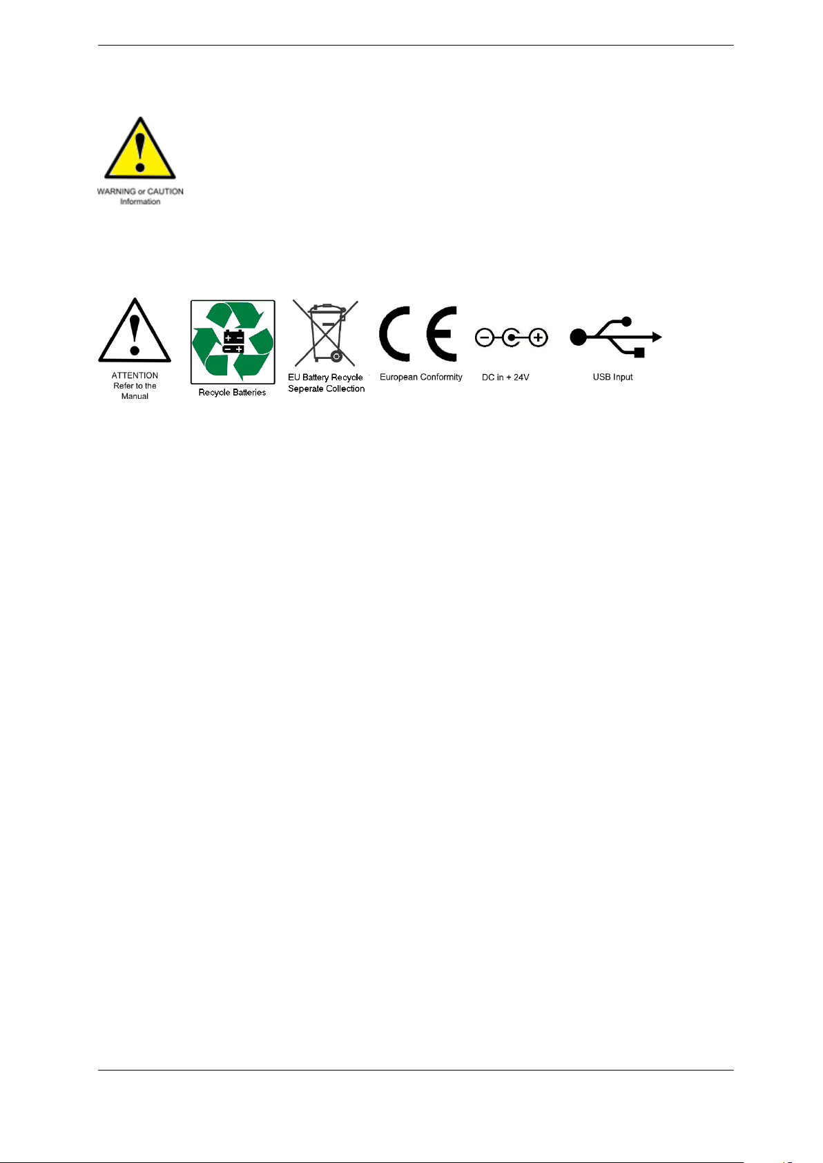
2.3. Symbols in the Manual

2.4. Symbols on the CT100B

2.5. Static Charge

Any cable or wire can carry a significant static electric charge that could damage the sensitive
internal electronics of the CT100B. For this reason, it is essential to discharge the electrical
conductors of any cable or device-under-test (DUT) by shorting them to each other or to earth
ground before connection is made to the CT100B’s sampling circuitry.

CT100B instruments supplied with a front panel BNC test port are equipped with a built-in
internal self-grounding connection that briefly shorts the conductors of the DUT to each other,
dissipating stored charge, before completing the connection to the CT100B’s sensitive internal
sampling circuitry. For this reason, the last cable connection should always be made to the
CT100B test port. For example, if the DUT is a cable assembly, all internal connections within
the cable assembly should be made before connection is made to the CT100B BNC test port.
This ensures that all stored charge in the DUT is discharged during the connection to the
CT100B BNC test port.

Sometimes it is convenient to insert a patch cable between the CT100B BNC test port and the
DUT. In this case, it is recommended that all cable connections, including the connection of the
patch cable to the DUT, be made before connecting the patch cable to the CT100B BNC test
port. Otherwise, the BNC test port self-grounding safety feature is circumvented.

If for some reason the last connection cannot be made at the CT100B test port, then the
conductors of the DUT should be discharged (shorted) manually using an industry-standard
shorting cap termination or equivalent direct electrical connection.

Note that CT100B instruments equipped with SMA or other front panel test ports do not have
internal self-grounding protection. Therefore, when using these instruments, the conductors of
the cable under test/DUT should always be shorted to each other or to earth ground prior to
connection to the CT100B’s test port.

4 CT100B TDR Cable Analyzers Operator’s Manual

2. Safety Summary

CAUTION: Failure to properly ground the cable/device under test prior
to connecting it to the front panel connector, either directly or indirectly,
could result in damage to the sampling electronics and will void the War­ranty.

2.6. Fuses

There are no external fuses or breakers accessible to the user. However, there are two internal
automatic thermal breakers that disconnect the power from the charger and battery to the rest
of the system. These thermal breakers make an audible click when they actuate, and the
CT100B turns off. One of the circuit breakers automatically resets after time. When this
breaker cools, the CT100B can be restarted, but the CT100B should be serviced by qualified
personnel. There is also an internal breaker on the power board. If tripped, this breaker must
be reset manually and the instrument should be serviced by qualified personnel.

CAUTION: If the thermal breakers trip, the instrument should be evalu­ated by qualified service personnel for maintenance.

2.7. AC Power Source

The CT100B is intended to operate only from a 120 VAC or 240 VAC RMS power source using
the CE- and UL-approved 24 VDC external power supply/adapter (pn: CT100-AC-PS)
provided with the instrument.

WARNING: Only use the power cord supplied with the instrument, and
then only if the cord is in good condition. Refer all maintenance regarding
the power supply or power cord to qualified service personnel.

CAUTION: Use of any power source other than the supplied external
power adapter(s) could damage the instrument and may void the War­ranty. Use only MOHR-approved accessories.

WARNING: To reduce the risk of electric shock, disconnect all external
cables before connecting the 24 VDC external power supply.

CT100B TDR Cable Analyzers Operator’s Manual 5

2. Safety Summary

2.8. Grounding the CT100B

When the CT100B is connected to the external AC adapter, the CT100B chassis, front panel
USB, screen, and controls are grounded through the grounding conductor of the power cord. To
avoid electrical shock, it is essential that the protective ground connection is present when
operating the unit under AC power. When disconnected from external power, the CT100B is
floating relative to earth ground, unless one of the USB ports is connected to a grounded device.
In this case, the ground of the USB device is common with the CT100B chassis, screen, and
electronic controls. An isolated ground power supply is an optional accessory available upon
request.

At all times, the front panel BNC or SMA connector is floating and is isolated by at least 500
VDC from the remainder of the CT100B. This eliminates measurement errors caused by
common-mode noise and slight ground-potential differences in the cable/device under test.
However, care should be taken with respect to electrical safety, as the front panel BNC or SMA
shield is never safely grounded unless connected to a safely grounded cable or device and can be
considered a second live conductor if connected to a cable or device carrying a non-zero
electrical potential relative to earth ground. This situation carries the risk of electric shock.

WARNING: The BNC or SMA connector shield represents a floating
ground and is never safely grounded even with the use of a properly
grounded AC adapter. Never use the CT100B to test any cable or de­vice carrying a non-zero electrical potential relative to earth ground, as
this could render an electric shock.

2.9. Danger Arising From Loss of Ground

When disconnected from the AC power adapter, the CT100B is no longer grounded unless
connected to a grounded USB device at the front panel host USB port. Because the test port
connector shield is floating relative to the remainder of the instrument, the test port connector
may be operating at an elevated voltage even when the AC adapter is connected. Therefore, the
test port connector should never be used to test any cable or device with an electrical potential
relative to earth.

WARNING: Upon loss of the protective-ground connection, all accessible
parts, including the screen, knobs, and connectors, can render an electric
shock.

2.10. Explosive Atmospheres

Do not operate the CT100B in an explosive atmosphere unless your unit has been specifically
certified for that condition. Explosive Atmospheres: MIL-STD 810G, Method 511.5, Procedure I
(+55◦C, sea level to 4600 m).

6 CT100B TDR Cable Analyzers Operator’s Manual

2. Safety Summary

2.11. Do Not Remove Covers or Panels

To avoid personal injury and risk of electric shock, do not open the CT100B case unless
replacing the battery and do not operate unless the case is fully intact.

WARNING: Disconnect power, USB, Ethernet, and test cables prior to
opening the CT100B case to replace the battery. Failure to do so can
render an electric shock.

2.12. Connecting Cables to the Test Port

To avoid damage to the CT100B and the very sensitive sampling electronics associated with the
front panel BNC or SMA connector, do not connect it to any cable or device that can be driven
by active circuitry or is subject to transient voltage spikes.

WARNING and CAUTION: The instrument should never be used to test
any cable or device carrying live electrical signals, as this carries a risk of
electric shock. This could also damage the sampling electronics and will
void the Warranty.

CAUTION: Always properly ground the conductor(s) of any cable or
wiring to remove any static charge prior to connecting it, either directly
or indirectly through attachment to another cable, to the CT100B’s front
panel test port connector. Failure to do so can damage the instrument’s
sensitive sampling electronics and will void the Warranty.

2.13. Battery Replacement and Disposal

The CT100B contains an internal battery pack. The internal battery pack is 2700 mAh, NiMH,
12 AA cells, 14.40 volts, 38.88 Wh. There is also a 120 mAh lithium button cell of 2.8 volts and

0.336 Wh. Depending on the state or local jurisdiction, these batteries may require special
disposal and/or recycling. Contact your local authorities for safe disposal in your area, or you
may return them to MOHR for recycling.

WARNING: The battery pack must be replaced with MOHR pn: CT100­AC-B2700. Use of any other battery pack will damage the instrument and
pose a danger of fire.

CAUTION: User replacement of components is limited. Multiple war­ranty seals are installed on components within the CT100B. Removal or
damage of these seals voids warranty.

CT100B TDR Cable Analyzers Operator’s Manual 7

3. Operating Instructions

3.1. Overview

If you would like a detailed explanation of TDR measurement theory and applications before
using the CT100B, please read Section 5, TDR Measurement Theory.

3.1.1. Handling

The CT100B is designed to meet the rigors associated with normal instrument use both in the
field and on the benchtop. Care should be taken to protect it from excessive mechanical shock,
vibration, static electrical charges, and water hazards.

The CT100B front panel is protected from impact by a snap-on front cover. The carrying
handle rotates 360° and can be used to support the instrument for bench-top use.

The CT100B is not watertight and must be protected against water spray. If the unit is
subjected to water spray, first turn off the unit with the battery-disconnect power switch on the
rear panel and then drain all of the excess water from the case and allow it to dry completely.

As noted in the Safety Summary and elsewhere, the CT100B is sensitive to damage introduced
by electrostatic discharge. Always properly ground the conductors of a cable to each other or to
earth ground before attaching it, either directly or indirectly, to the front panel BNC, SMA, or
other test port. Failure to do so could damage the sampling electronics and void the Warranty.

The CT100B can be stored in temperatures of between -20°C to +60°C with or without a
battery installed and can be operated from 0°C to +50°C.

3.1.2. Powering the CT100B

The CT100B can be powered through the included 120/240 VAC (RMS) to 24 VDC external
power adapter. This adapter has sufficient capacity to charge the internal battery from a dead
battery state while the unit is under operation. The internal battery will allow the unit to
operate using power conservation techniques for periods of at least 6 hours under typical use.
Automatic power-down occurs after a variable amount of time of inactivity, selectable in
software by the user. The screen also can be set to turn off after a set amount of inactivity. A
heavily discharged battery will require 4 hours to reach full charge.

Fusing is internal and based on thermal reset switches and a manual-reset breaker. If one of
these fuses trips, it may indicate that a hardware malfunction has occurred and the instrument
should be evaluated by qualified personnel.

CT100B TDR Cable Analyzers Operator’s Manual 9

3. Operating Instructions

3.1.3. Caring for the Battery

The CT100B has an intelligent battery-charging circuit that dynamically determines the
optimum charge rate and reverts to low-level trickle charge when the battery is fully charged.
Charging is automatic and there are no charge-length restrictions.

The battery should be charged between 0◦C and +45◦C. Battery operation should be limited to
between 0◦C and +50◦C. Batteries should be stored between -20◦C and +60◦C. If the battery
pack is older, it may not show a 100% charge capacity even when the maximum battery charge
is obtained.

CAUTION: Do not attempt to charge the battery pack below 0◦C or above
+45◦C. Batteries should not be stored below -20◦C or above +60◦C.

3.1.4. Charging and Power Status

The CT100B operates from a 24 volt power adapter or the internal battery pack.

In the Power menu, a submenu of the Settings menu, the user can set power save and shutdown
timers. Different timeout values can be set for when the CT100B is using the AC/DC converter
or batteries. In power save mode, the screen goes blank and only enough power is used to
monitor for user input. When input is received, the CT100B resumes normal operation. When
the shutdown timer expires, the CT100B will turn off.

A battery indicator can be toggled on or off with the Power Display menu option in the Power
menu. The indicator will show the level of charge in the battery. It will also show if the 24 volt
adapter is attached and providing power.

3.1.5. Batteries and Long-Term Storage

The CT100B has NiMH internal batteries. These batteries will drain if the CT100B is left in
storage over long periods. To preserve battery charge for as long as possible during storage,
make sure the power switch on the back of the CT100B is set to the OFF position. After several
months of storage, the internal batteries may be completely drained. Allow up to 4 hours for the
first recharge of the CT100B after coming out of long-term storage.

3.1.6. Low Battery

When a low battery condition is first encountered, the CT100B alerts the user. Internal
Battery Low text appears on-screen in red when the battery percentage left drops below 20

percent.

10 CT100B TDR Cable Analyzers Operator’s Manual

3. Operating Instructions

3.1.7. Nameplate

The CT100B has a nameplate label affixed on the back of the case. See Figure 3.3 for
positioning. The nameplate includes Cage Code, Model Number, Serial Number, NSN, a
warranty expiration date, electrical input information, and a 2D barcode containing the
identifying information. See Figure 3.1 for an example nameplate label.

Figure 3.1. Example nameplate label found on back of a CT100B.

3.1.8. Discharge Warning Label

The CT100B has a warning label above the test port on the front of the instrument. This label
warns the user to discharge any cable or device before connecting it to the test port.
See Figure 3.2 for location and contents of the label.

3.2. License Codes

Each CT100B requires a unique license code to operate. Without the correct code, menus and
buttons still function, but there will be no live trace displayed on the screen. The correct code
for a particular device can be requested from MOHR. Installation instructions will be included
with the license code.

Depending on how it was purchased, the instrument may be supplied with either a 30-day
demonstration license or permanent license. Current license information can be found by
pushing the blue MENU button and navigating to Settings → Info → License → License Info.
A dialog showing license date and active features will appear. When the CT100B has a
permanent license installed, appropriate options will be active. When the instrument has a
demonstration license, the dialog will show a future license date and the instrument will provide
appropriate warnings to the user as the expiration date gets closer. If your CT100B has a
license with pending expiration and you are unsure how to upgrade to a permanent license,
please contact MOHR.

3.3. Preparing to Use the CT100B

Before using the CT100B, make sure you have read and understand the Safety Summary section
and power requirements described in Section 3.1.2 through Section 3.1.6. If you would like a
detailed explanation of TDR measurement theory and applications before using the CT100B to
test cables, please read Section 5, TDR Measurement Theory.

CT100B TDR Cable Analyzers Operator’s Manual 11

3. Operating Instructions

Otherwise, remove the front cover and turn on the power. You are ready to test cables using the
most versatile and sophisticated portable TDR instrument on the market.

3.4. Front Panel Controls and Connectors

The following numbered items describe the controls and connectors identified in the front panel
diagram (Figure 3.2) and described in the text below.

Figure 3.2. Diagram of the CT100B front panel.

1. POWER (red) button. Pressing this button turns the instrument on when the main
power switch on the rear panel is in the ON position. Pressing the POWER button when
the unit is on will turn the unit off after verification that you really wish to power down. If
the POWER button is held in for several seconds, the unit will turn off regardless.

2. H1 function button. Function depends on menu.

3. H2 function button. Function depends on menu.

4. H3 function button. Function depends on menu.

5. H4 function button. Function depends on menu.

6. MENU (blue) button. Push to display the top-level menu screen. If a menu is already on
the screen, this button will clear the menu. The previous menu will be displayed. This
button also activates on-screen help when held down while pressing other buttons.

7. VERTICAL POSITION knob. Controls the vertical position of the currently selected
trace. Trace selection is controlled by the SELECT button (14).

8. VERTICAL SCALE knob. Controls the vertical scale, which is displayed on the bottom of
the screen. This control modifies the appearance of the currently selected trace. The scale
is expanded about the vertical center of the screen.

9. HORIZONTAL POSITION knob. Controls the horizontal position of the active cursor.
Displayed trace positions are moved horizontally if the cursor is moved toward the edge of
the screen to keep the cursor on-screen.

10. HORIZONTAL SCALE knob. Controls the horizontal scale of displayed traces. The scale
is expanded about the active cursor.

12 CT100B TDR Cable Analyzers Operator’s Manual

3. Operating Instructions

11. BNC or SMA test port. This connects to the cable to be tested. Be sure to properly
ground the cable before connecting it to test port in order to prevent electrostatic damage
to the CT100B’s sensitive sampling circuitry.

CAUTION: All static charge must be drained from the cable to be tested
prior to connecting to the test port (11). This is done by shorting the cable
center conductor to the cable sheath/ground return. If this procedure is
not fol lowed, the sampling electronics can be damaged and will void the
Warranty.

12. Host USB port. This USB (V1.1) connection can be used to interface to a client USB
device such as a barcode reader, keyboard, or flash drive.

13. FILE button. Opens the File menu, which contains a database of user configurations,
saved cable records (scans), and a Vp database for known cable types.

14. SELECT button. Used to select between traces on the screen. It has no effect if there are
no other traces. Note: When the SELECT button is held down, press the M-FUNC
button. The CT100B will generate a screenshot that can be saved to a USB drive.

15. CURSOR button. This button is used to toggle between the two available cursors.
Pressing and holding the CURSOR button for one second and then releasing the button
will bring both cursors onto the screen.

16. SCAN button. Displays a specialized soft-menu that brings up the Scan menu.

17. AUTOFIT/HELP (orange) button. Opens the on-screen help library along with Autofit
soft-menu options.

18. M-FUNC (multifunction) button. The function of the M-FUNCTION knob (19) is set by
this button. The current operation is displayed on the screen (top-center).

19. M-FUNCTION (multifunction) knob. This knob adopts the function selected through the
use of the M-FUNC button (18). It also allows users to scroll through dialog box options.

20. V1 function button. Function depends on menu.

21. V2 function button. Function depends on menu.

22. V3 function button. Function depends on menu.

23. V4 function button. Function depends on menu.

3.5. Rear Panel Connectors and Switches

The following numbered items describe the connectors and switches identified in the rear panel
diagram (Figure 3.3) and described in the text below.

24. 24 VDC power adapter plug. The provided 24 VDC AC adapter plugs into this port. Only
MOHR-approved positive center tip, 24V adapters may be used.

25. Client USB connection. Allows the CT100B to be connected to a host computer for data
transfer and PC control.

26. RJ-45 Ethernet port. This is a 10/100 Mb Ethernet port that can be used for data
transfer and remote PC control.

27. Power switch. This is a manual ON/OFF power switch that turns the device off and
disconnects the power from the internal electronics so the unit can be stored and/or
shipped safely.

CT100B TDR Cable Analyzers Operator’s Manual 13

3. Operating Instructions

Figure 3.3. Diagram of the rear panel of the CT100B/CT100HF.

3.6. Keyboard Alternate Controls

If a keyboard is plugged into the front panel USB port, alternate hotkey controls are available
for all front panel buttons and knobs.

1. F1-F4 map to H1-H4.

2. F5-F8 map to V1-V4.

3. F9 maps to the blue MENU button.

4. F10-F12 map to the M-FUNC, SCAN, and SELECT buttons.

5. Shift F10-F12 map to AUTOFIT/HELP, CURSOR, and FILE.

6. Vertical arrow keys adjust the VERTICAL POSITION knob.

7. Horizontal arrow keys adjust the HORIZONTAL POSITION knob.

8. Shift vertical arrow keys adjust the VERTICAL SCALE knob.

9. Shift horizontal arrow keys adjust the HORIZONTAL SCALE knob.

10. Shift F7 rotates the M-FUNCTION knob counter-clockwise.

11. Shift F8 rotates the M-FUNCTION knob clockwise.

Note: Some functions may require multiple button pushes to take effect.

3.7. Setting up the CT100B

3.7.1. Setting Date and Time

The date, time, and time zone must be accurately set for saved data in the CT100B to be
correctly time-stamped.

1. Change the date and time by pressing the MENU button. This calls up the Main menu.

2. Select the Settings soft-menu option and then select the Info menu.

3. Select the Time menu option. The Time menu appears.

4. Select the Set Time Zone menu option. A dialog box listing all time zones appears on the
screen.

5. Use the M-FUNCTION knob to scroll through the list of time zones. Highlight the correct
time zone.

14 CT100B TDR Cable Analyzers Operator’s Manual

3. Operating Instructions

6. Choose the Select menu option. The CT100B may prompt you to restart. If so, restart the
unit and return to the Time menu. The CT100B is now set to the correct time zone.

7. Ensure the menu option for daylight savings reads Daylight Savings On, indicating that
this setting is on. If the option reads Daylight Savings Off, then press the menu button to
toggle it. The CT100B may prompt you to restart. If so, restart the unit and return to
the Time menu. The CT100B will automatically adjust for daylight savings on the correct
dates.

8. Select the Time/Date menu option. A dialog box used to set the date and time appears.
See Section 3.7.2 for methods of navigating and entering data into a dialog box.

9. Press the OK menu option when the correct time and date have been entered.

3.7.2. Navigating Dialog Boxes

For an example of a dialog box with multiple entries, press the blue MENU button, then
Settings, then Info, then Time, and then Time/Date. Scroll through the different entry boxes

with the M-FUNCTION knob. With an entry box selected, press the Show Keyboard menu
option to call up an on-screen keyboard.

With the on-screen keyboard chosen, select the desired characters with the M-FUNCTION
knob, pressing the Select Highlighted menu option for each one. Get more character options by
selecting the Shift menu option. Delete the character before the cursor with the Backspace menu
option.

With the keyboard open, accept the current entry with the Hide Keyboard menu option or
revert to the original entry with the Cancel menu option. Both options remove the on-screen
keyboard from the screen.

With the keyboard off the screen, select the OK menu option to accept all changes to the
current dialog box and close the dialog box. Select the Cancel menu option to close the dialog
box while canceling all changes.

With a USB keyboard attached, entries can be changed directly. Use the Tab key to scroll down
through entry boxes and hold down Shift and press Tab to scroll up through entry boxes. Use
Backspace to delete the character before the cursor and use the arrow keys to move the cursor
left or right. Press Enter for OK or Escape for Cancel.

3.7.2.1. Scrolling Dialog Boxes

Some dialog boxes present a list of items to be selected. For an example of this type of dialog
box, press the FILE button, and then press Cable Scan Records (see 3.11.8 and Figure 3.23).
Use the M-FUNCTION knob to highlight individual items for selection, and then use the Select
option to choose the highlighted item. Where appropriate, multiple items can be marked for
selection using the options on the right-side menu: Toggle Selected, Clear All, and Mark All.
When an individual item is marked, it will appear in a different color.

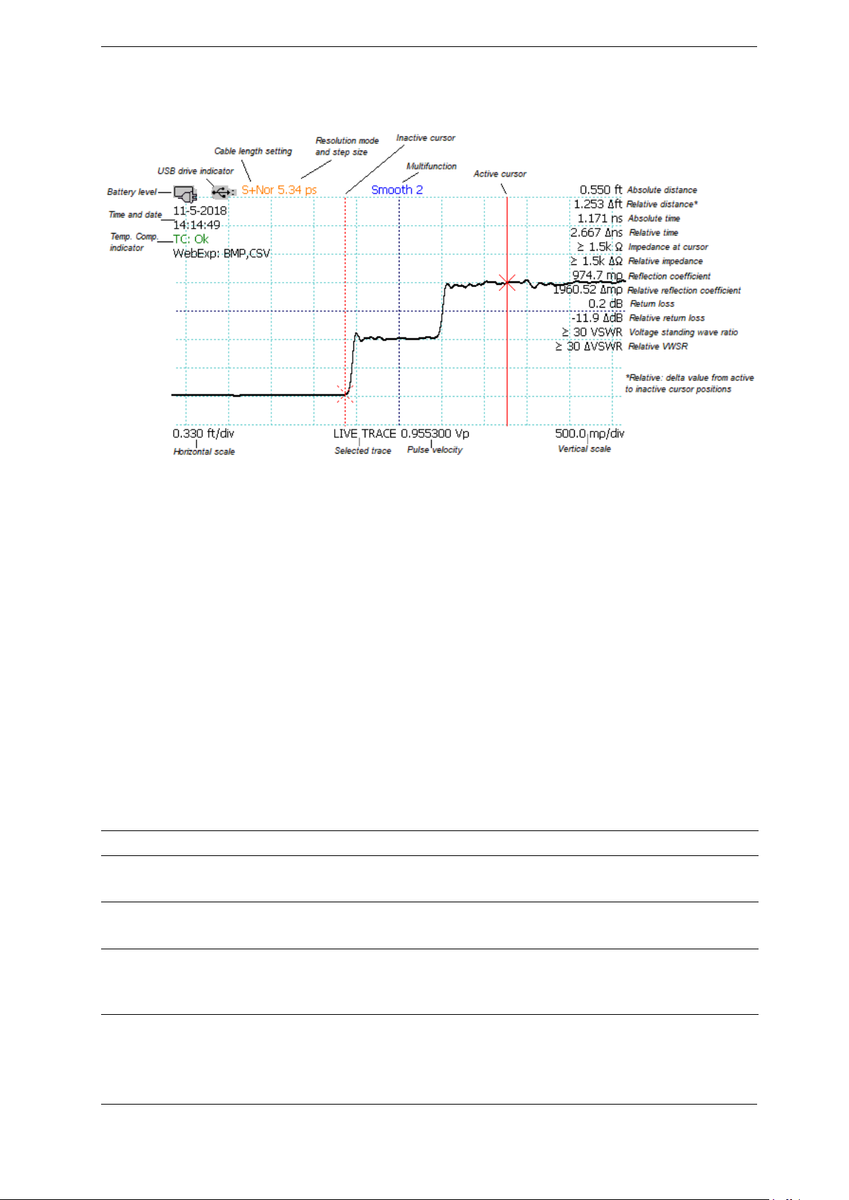
3.8. Display Features

The CT100B screen provides the operator with numerous features that may be useful in
different cable testing situations. Figure 3.4 shows some of the typical features you will

CT100B TDR Cable Analyzers Operator’s Manual 15

3. Operating Instructions

encounter during use. Many other features are available, however, and most of them are
configurable by the user. These features are described in detail in the following sections.

Figure 3.4. Screenshot showing typical features of the CT100B.

3.9. Menu Selections and Function Buttons

3.9.1. M-FUNC Button

The M-FUNC button is used to switch between functions Shift, Smooth, and Vp (and
Fine/Coarse Vp) shown in the Multifunction indicator at the top of the display screen.

3.9.2. SCAN Button Menu

The SCAN button displays menu selections associated with saving and managing TDR traces
and cable scan records. SCAN menu selections are shown in Table 3.1.

Table 3.1. SCAN Button and Menu.

Menu Selection Purpose/Action

Save/Rename Saves selected trace to internal storage. Renames

previously saved traces.

Show Sel. Trace Only Turns all traces invisible except the currently

selected trace. Select again to set all traces visible.

Hide All Traces Hides all traces except the live trace. (If traces were

previously saved, they can be recalled from the FILE
menu; see Section 3.9.6)

16 CT100B TDR Cable Analyzers Operator’s Manual

3. Operating Instructions

Table 3.1 (Continued) SCAN Button and Menu.

Menu Selection Purpose/Action

Hide Selected Trace Hides the selected trace. (If trace was previously

saved, it can be recalled from the FILE menu; see
Section 3.9.6)

Start Scan Initiates cable scan.

Cursor/Snapshot Switches between scan modes:

Cursor ........................... Creates a new scan of the portion of trace between

cursors using the current resolution and smooth
settings.

Snapshot ......................... Saves trace as currently displayed on screen.

Math See Table 3.2: Math Menu.

Table 3.2. Math Menu

Menu Selection Purpose/Action

FFT Tools

FFT Settings

Window Sets window type (Hann, Hamming, etc.).

size FFT buffer size.

Frequency Cut-Off Range FFT display frequency cut-off.

Hide Selected Trace Hides the selected trace.

Apply FFT Creates FFT trace from selected trace data.

View Live FFT Creates live FFT trace from live TDR trace.

Apply VSWR Creates VSWR (voltage standing wave ratio) trace

from a selected complex division or S11trace.

Set Base Sets base trace for complex FFT trace division.

Complex Division Creates complex division FFT: Divides selected FFT

by base FFT. Equivalent to uncalibrated S11trace
when base FFT is of a shorted test port.

Phase Creates phase angle trace from selected FFT trace.

Smith Chart Toggle Smith Chart display for selected complex

division FFT or S11trace.

SParam & Normalize Tools

S11Calibration Performs Open-Short-Load S11calibration and

creates S11trace.

Normalize Pulse Rise Time Sets the rise time to apply to the selected normalized

trace.

S11Options

CT100B TDR Cable Analyzers Operator’s Manual 17

3. Operating Instructions

Table 3.2 (Continued) Math Menu

Menu Selection Purpose/Action

Pre-Filter Options Changes the filter options that smooth the

aberrations of the base traces.

Post-Filter Options Changes the filter options that limit the noise of the

base traces.

Other S11Options

OSL Bases Visible When enabled, causes the Open, Short, and Load

traces to not appear on-screen. Helps eliminate
excess on-screen clutter.

Align Base Traces When enabled, the Open, Short, Load, and DUT

traces may be aligned to each other based on the
common part of the beginning of the trace.

Calibration Standards Brings up a table of Calibration Standard Kits

Coefficients. There is the option to change and apply
the standards.

S11→ USB (.csv) Creates a CSV (Comma Separated Value) file of the

selected S11trace and outputs that file to a
connected USB drive.

Phase Corr. Off/On Toggles the Phase Correction On/Off.

Phase Corr. Start Using the active time-domain cursor, sets a new

start point for the Phase Correction.

Between Cursor Off/On /Hold Toggle S11Between Cursors mode:

Off............................ Between Cursors Off.

On............................. Between Cursors On – the active section will adjust

with time-domain cursor movement.

Hold .......................... Between Cursors Hold – the active section will

remain regardless of cursor movement.

Hide Selected Trace Hides the selected trace.

Reapply S

11

Adjusts the time-domain settings to match those
used for the selected live S11trace.

Apply Normalization Create normalized TDR trace based on the selected

S11trace.

Cable Loss Changes selected S11trace to Cable Loss

(S21/insertion loss) trace. Terminate cable with
precision short adapter for meaningful results.

Smith Chart Toggle Smith Chart display for selected complex

division FFT or S11trace.

Layer Peeling Create layer peeling trace from selected trace.

Assumes active cursor (layer peel start) is set at 50
ohms.

Hide Selected Trace Hides the selected trace.

18 CT100B TDR Cable Analyzers Operator’s Manual

3. Operating Instructions

Table 3.2 (Continued) Math Menu

Menu Selection Purpose/Action

Set Base Sets selected trace as the base (denominator) trace

for math operations.

Difference Creates subtraction trace from selected trace and

base trace (Difference = Selected – Base).

1st Derivative Creates first derivative trace from selected trace.

Der. Smooth Off/On Toggles first derivative trace smoothing.

3.9.3. SELECT Button

The SELECT button switches which trace on-screen is the active trace. See Section 3.11.6 for
more information on selected traces.

3.9.4. AUTOFIT/HELP Button

The AUTOFIT/HELP button calls up the online help library and AUTOFIT soft-menu
options. Use the M-FUNCTION knob and Select menu option to scroll through and select the
help library content. When you select the AUTOFIT menu option, the CT100B looks for the
TDR signature of an open or short-terminated cable and selects appropriate horizontal and
vertical scale values to display the entire cable on the screen. By default the cursors are
positioned approximately to the beginning and end of the cable.

If Vertical Recenter is selected then only vertical scale and position are affected.

3.9.5. CURSOR Button

Toggles between cursors, making the active cursor inactive and the inactive cursor active.
Pressing and holding the CURSOR button for one second then releasing will reposition any
cursors not visible on the screen to the screen.

3.9.6. FILE Button and Menu

Use this menu to access the user library of configurations, cable types, and cable records. FILE
button menu selections are shown in Table 3.3.

Table 3.3. FILE Button and Menu

Menu Selection Purpose/Action

Custom Cable Types Use to add, select, or delete an entry from the

custom cable type library:

Add New .......................... Enter in new cable type information.

Delete............................ Delete selected cable type from the library.

Select............................ Select the highlighted custom cable type. Instrument

settings change to reflect the cable Vp setting.

CT100B TDR Cable Analyzers Operator’s Manual 19

3. Operating Instructions

Table 3.3 (Continued) File Menu

Menu Selection Purpose/Action

Reference Cable Types Use to select a built-in cable type from the standard

cable type library. Instrument settings change to
reflect the cable Vp setting.

Cable Scan Records Use to select, delete, or USB save a previously saved

TDR trace. (See Section 3.11.8 for more.)

Config Entries Use to add, select, or delete an entry from the user

configuration library.

Export CSV → USB Export selected TDR trace as a CSV file to USB

drive.

Save Scan Saves selected trace to internal storage.

Masks

Create Mask From Trace Generates mask or test limit based on the selected

trace.

Change Vertical Margin Adjusts vertical pass/fail criteria of the mask.

Change Horizontal Margin Adjusts the horizontal pass/fail criteria of the mask.

Clear Mask Removes the current mask from the display.

Masks Use to add, select, or delete a mask from the mask

library.

Print Screen Prints directly to a PCL3 compatible printer via

USB.

3.9.7. “Blue” MENU Button and Top-Level Menu

If no menu is displayed, the blue MENU button loads the main top-level menu. If the top-level
menu is displayed, it closes the menu. If a submenu is displayed, it displays the parent menu.
Top-level menu selections are listed below in Table 3.4. Holding down the MENU button while
pressing any button (or the M-FUNCTION knob) will display a help dialog for that button’s
current menu selection (known as “blue button help”).

Table 3.4. MENU Button and Menus

Menu Selection Purpose/Action

Cable Len Adjust the pulse timing for different length cables:

Short............................. For cables of up to approximately* 300 ft. (90 m)

long.

Medium............................ For cables up to 1500 ft. (450 m) long.

Long.............................. For cables up to 6,000 ft. (1,800 m) long.

[Note: Access Extra Long mode in the
Measurement submenu. Use Extra Long mode for
cables over a mile (2 km) in length.]

*The exact length will depend on the Vp setting.

20 CT100B TDR Cable Analyzers Operator’s Manual

3. Operating Instructions

Table 3.4 (Continued) MENU Button and Menus

Menu Selection Purpose/Action

Resolution Sets TDR trace horizontal sampling resolution (in

picoseconds):

Normal............................ A setting suitable for connector level detail for each

of the cable length modes. Short is nominally 5.32 ps
(< 1 mm). Medium is nominally 17.5 ps (~2 mm).
Long is nominally 49.6 ps (~1/2 inch). Extra Long is
nominally 381 ps (~2 inches). The actual setting is
dependent on horizontal scale, but will be at least as
good as the nominal value. If the user adjusts the
Horizontal Scale to zoom in to a very short section of
cable, the resolution setting will automatically adjust
to a finer scale. Multiple measurements may map to
a single horizontal offset on the display. This allows
you to easily see flaws in the cable or connectors
even when looking at long sections (see Figure 3.10).

Screen............................ Screen resolution (1 sample/pixel) varies

dynamically with the current horizontal scale.

Fixed............................. Allows user to set a specific value no matter the

cable length setting.

File (Load/Save) Calls up the FILE button menu. Use it to add,

select, or delete an entry from the cable type, user
configuration, and/or cable record libraries.

Connect to CT Viewer

Find CT Viewer Search the local area network looking for running

CT Viewer 2 programs. If successful, it establishes a
connection.

Manual Connect A dialog with a list of PCs that have previously been

added is displayed.

Add PC.......................... Enter in new server IP information.

Edit............................ If connected to CT Viewer 2, allows user to edit PC

name.

Delete.......................... Delete selected server from the library.

Select.......................... Connect to the highlighted server.

Cancel.......................... Cancel out of the connection menu.

See Section 4: CT Viewer for instructions on
connecting the CT100B to CT Viewer 2.

Use USB Go to the PC on which you are running CT Viewer

2 and use that program to connect to the CT100B.

SParam Tools Tools for creating S-parameter traces and normalized

traces. See Return Loss (S11) Traces in
Section 3.11.17 on page 49.

Measurement

Vert. Ref.

CT100B TDR Cable Analyzers Operator’s Manual 21

3. Operating Instructions

Table 3.4 (Continued) MENU Button and Menus

Menu Selection Purpose/Action

Vert. Ref Off/On Toggles VR (Vertical Reference) mode on/off.

Set Vert. Ref. Performs VR calibration using short/open

terminators. When setup is complete, a green
vertical line indicates start of VR measurements.

Vert. Ref. Center Imp. Adjusts VR calibration to use impedance matching

adapters and baluns.

Vert. Ref. Start Sets start of VR at the position of the active cursor.

Vert. Ref. End Sets end of VR at the position of the active cursor.

Cable Segments

Add New Segment Create a new segment boundary at the active cursor.

The selected segment will be split in two, each with
the same initial Vp.

Delete Segment Delete the currently selected segment. The segment

will be merged with the segment to the left.

Delete All Segments Delete all segments. The CT100B will return to

normal operation. A single Vp now applies to the
entire trace.

Prev Segment Select the segment to the left of the currently

selected segment.

Next Segment Select the segment to the right of the currently

selected segment.

Reset All Vp Reset the Vp of all segments to 1.000.

Restore All Vp Restore Vp of all segments to the previous values.

Extra Long Mode Extra Long Mode allows the CT100B to obtain

traces out to 40,000 ft. (12,000 m) (assumes
Vp=0.66). Extra Long Mode is slower than other
cable lengths and some instrument features are not
available. When in Extra Long Mode, the Cable
Length menu option will indicate Extra Long Mode
On. Selecting the cable length menu item will switch
off Extra Long Mode.

Vert. Units Select vertical units for a time-domain trace from

reflection coefficient (mρ), impedance (Ω) or voltage
standing wave ratio (VSWR). A few features of the
CT100B only work with the reflection coefficient
setting.

Envelope Plot Captures transient cable and connector faults.

Envelope Plot Off/On Enable/disable envelope plot mode. When turned on

the CT100B begins capturing trace data and
displaying envelope plot information.

22 CT100B TDR Cable Analyzers Operator’s Manual

3. Operating Instructions

Table 3.4 (Continued) MENU Button and Menus

Menu Selection Purpose/Action

Reset Deletes/restarts captured TDR trace envelope data.

Fill Mode Off/On Toggles between fill and probability density plot

mode. Use fill mode to find magnitude of impedance
change and highlighting fault location. Use
probability density plot mode to find infrequent
transient faults.

Hold Off/On When Hold is on, trace controls are locked for an

envelope plot. When Hold is off, trace controls work
normally.

Clear Historic As trace controls are used to change an envelope

plot, the envelope plot preserves a record of the trace
from previous positions. Clear Historic erases this
history, leaving only the plot from the current
position.

(Horizontal Units) Toggles through horizontal units (meters, inches,

feet, yards, centimeters)

Meas. Settings

Horiz. Units Toggles through horizontal units (meters, inches,

feet, yards, centimeters)

RRC Classic/1502C Mode Classic: Referenced to amplitude at inactive cursor.

1502C: Referenced to amplitude at test port.

Vp 3/6 Sig Figs Toggle Vp significant digits from 3 to 6 digits.

Vertical Correction

Adjust mρ Offset Allows manual vertical measurement offset

adjustments. This allows advanced users to
manually calibrate impedance measurements at a
particular location to a known value.
When activated the M-FUNCTION knob adjusts
the vertical offset. The blue M-FUNC indicator
shows the offset in mρ (millirho).

Cancel mρ Offset Use this option to cancel a manual mρ (millirho)

correction. Automatic temperature adjustment will
resume auto-correction of the vertical measurements.

Adjust Ω/(unit) Use the M-FUNCTION knob to change the ohms

per unit distance resistive loss setting until the cable
shows no upward or downward trend across its
length.

Ω/(unit) Correct. On/Off Toggle resistive cable loss correction on/off, as

described above. If the end point of the correction
has not been set, then it will be set to the position of
the active cursor.

CT100B TDR Cable Analyzers Operator’s Manual 23

3. Operating Instructions

Table 3.4 (Continued) MENU Button and Menus

Menu Selection Purpose/Action

Set Ω/(unit) Pos. Set the position of the ohms/(unit distance) position

to that of the active cursor.

Clear Reset all Ω/(unit) settings.

Math See Table 3.2: Math Menu.

Settings

Meas. Settings See Meas. Settings under Measurement menu above.

Network Settings

Static Network Settings Modify static network settings (if DHCP inactive):

IP Address . . . . . . . . . . . . . . . . . . . . . IP address (xxx.xxx.xxx.xxx)

Netmask . . . . . . . . . . . . . . . . . . . . . . . . Subnet for CT100B

Gateway (optional) . . . . . . . . . . . Gateway server setting

Nameserver 1 and 2

(optional) . . . . . . . . . . . . . . . . . . . . . . . . . .

Nameserver settings

DHCP on/off Toggles DHCP on/off.

Show IP Config. Displays current Ethernet configuration.

Web Export On/Fast/Off Activates and toggles function of web server into

three states: On, Fast Mode, and Off. The web
server provides .csv format files as well as screen
capture bitmaps. See Section 3.11.25 for more
details on accessing data using web export.

On............................. Normal operation (~2 frames/sec).

Fast Mode..................... Fast refresh (~7 frames/sec).

Off............................ Web server not active.

[Note: See Section 4 for more information on using
CT Viewer 2 to acquire TDR traces. See
www. mohrtm. com for information on the CT100B
Python programming library and binary programming
protocol for Ethernet CT100B interface.]

Selected .csv Options Opens a dialog for adding additional data columns

in the .csv trace export file.

Set Listen Ports This dialog box allows you to define a different RPC

port # and a different Remote Control Port # for
use with the CT Viewer 2 application (default 12347)

SP232 Protocol On / Off Toggles SP232 emulation on/off. A USB to serial

adapter is required for SP232 emulation. Press this
button while emulation is on to switch the baud rate.

Power

DC Power Save Sets the inactivity timeout for power save mode

while the device is running on external DC supply.

DC Shutdowns Sets the inactivity timeout for shutdown while the

device is running on external DC supply.

24 CT100B TDR Cable Analyzers Operator’s Manual

3. Operating Instructions

Table 3.4 (Continued) MENU Button and Menus

Menu Selection Purpose/Action

Battery Power Save Sets the inactivity timeout for power save mode

while the device is running on batteries.

Battery Shutdown Sets the inactivity timeout for shutdown while the

device is running on battery.

Battery Icon Toggles battery icon display on/off.

Power Display Toggles the on-screen power status display on/off.

Diagnostics

Analog Run automated diagnostics on the analog trace

acquisition circuit board. Results are displayed
on-screen in a message box.

Database Clean Database: CAUTION! Not for routine

use. This option defragments the database, freeing
up unused space, then turns off the CT100B. Use
this option only when the CT100B is plugged into an
external power supply. Do not shutdown the
CT100B while the Clean Database command is in
progress.

Front Panel Check This item opens the front panel button and knob

check screen. Hit each button once and turn every
knob in each direction. Press the red power button
to exit when finished.

Jitter Jitter measures signal noise, jitter, rise time, and

sampling efficiency of the trace. These values are
used as part of the calibration checkout for the
CT100B, and results of interest are explained in
Appendix B: Operating Performance Checks.

Calibration Performs vertical and horizontal calibration.

Info

License

License Info This option gives information about the license

installed on the CT100B.

License from USB Use this option to load a license code from a USB

flash drive.

Enter License Manually load a license code. This is useful for

operators who are unable to connect to CT Viewer 2
or use a flash drive.

Web Update When a CT100B is connected to the Internet, this

item will automatically update the CT100B if newer
software is available.

Update From USB Drive Will run an update from the connected USB drive.

CT100B TDR Cable Analyzers Operator’s Manual 25

3. Operating Instructions

Table 3.4 (Continued) MENU Button and Menus

Menu Selection Purpose/Action

Web Update Address View/set the web address to query for updated

software. Normally this setting should not be
changed.

Processor Displays CPU information.

Contact Contact information for MOHR.

Auto Update On/Off Toggles Auto-Update on/off. With Auto-Update on,

the CT100B will automatically check to see if it is
running the current software version and notify the
user if a new version exists.

Software Version Display software and firmware version information.

This also serves to verify the communications links
between the micro-controllers.

Hardware Info Display hardware information.

Usage Display instrument usage in hours.

Time Time and date settings:

Time Date Set the current date and time.

Set Time Zone Change the time zone.

Daylight Savings On Off Sets adjustment for daylight savings time on/off.

Display

Change Screen Profile Toggles screen background (black, gray, white).

Ohms/Rho Toggles display of impedance (ohms) and reflection

coefficient (millirho) at cursor and between cursors.

VSWR Toggles display of VSWR (voltage standing wave

ratio) at cursor.

Trace Labels On/Off Toggles display of the trace labels directly below the

traces.

Time/Date Toggles time/date display.

Distance/ns Toggles display of distance and time (ns) at cursor.

Temp Comp Toggles display of Temp Comp autocalibration

status.

Min/Max Display Toggles display of min/max values for high

resolution sampling.

Horiz. Vert. Ruler Toggles display of horizontal and vertical rulers.

Noise Value Toggles display of noise value at cursor for diagnostic

purposes.

Vert. Shift Correction Toggles the Vertical Shift Correction option. When

on, corrects the vertical shift that can happen when
changing the DUT.

26 CT100B TDR Cable Analyzers Operator’s Manual

3. Operating Instructions

Table 3.4 (Continued) MENU Button and Menus

Menu Selection Purpose/Action

Time of Flight Show Time of Flight time measurements. The

standard nanoseconds display shows electrical time
for a pulse to reach a point and then return to the
CT100B.
Time of Flight is exactly half that value. It is the
one-way transmission time.

Vert Centering On/Off When on, changes to vertical scale will center on the

point where the cursor intersects the selected trace.
When off, changes to vertical scale will center on the
center of the screen.

Draw Internal Cable Bkgrnd Changes the background of the trace beginning from

the start of the trace to the end of the internal cable.

Auto Smooth Reset On Off When on the CT100B will automatically reset

smoothing when a change in load is detected by the
device.

Scale Toggles display of horizontal, vertical scales, and Vp.

Intersection Toggles display of cursor-trace intersection.

Decibels Toggles display of decibel (dB) values at cursor.

Temperature Toggles display of instrument internal temperatures.

AutoSmooth On Off When on, the CT100B will automatically pick a

smoothing value based on the observed noise.
When off, the CT100B will use the user-entered
smoothed value.

3.10. Test Preparations

If you would like a detailed explanation of TDR measurement theory and applications before
using the CT100B to test cables, please read Section 5, TDR Measurement Theory, or go to
www.mohrtm.com.

3.10.1. Connecting to the Cable or Device-Under-Test (DUT)

The first and most important decision to make when testing a cable or device-under-test (DUT)
is how to connect to the DUT. Because the connection to the DUT acts as a filter for the test
signal into and out of the DUT, it is very important that the connection have the highest
bandwidth and least aberration possible.

Controlled impedance connections are recommended whenever possible. Controlled impedance
connections have conductors with uniform geometry and dielectric properties that do not change
significantly during a test session or between test sessions. Examples of controlled impedance
connections include coaxial-coaxial adapters, coaxial-twisted pair adapters, and fixed-pitch TDR
probes.

CT100B TDR Cable Analyzers Operator’s Manual 27

3. Operating Instructions

Alligator clip and clip lead adapters with flexible wire test leads should be used only as a last
resort. Alligator clip and clip lead adapters are not made for high frequency operation, are
severely bandwidth limiting, and introduce severe aberration and measurement uncertainty into
the TDR trace. Figure 3.5 shows a comparison test of a coaxial cable using clip lead adapters
(red, top) and a controlled-impedance adapter (black, bottom). The clip lead adapter TDR
trace is severely degraded.

MOHR is able to supply controlled-impedance adapters for almost every type of cable and
connector.

Figure 3.5. Clip lead adapter (red, top) and controlled-impedance adapter (black,
bottom) testing of 3 ft. coaxial cable with short termination. Active cursor is at the test
port. Clip lead adapters introduce severe TDR trace distortion.

3.10.2. Change Velocity of Propagation (Vp)

Vp is expressed as a fraction of the speed of light. The current setting for Vp appears on the
lower center of the screen. Press the M-FUNC button until the top-center information indicator
reads “Vp”. If Vp 6 Sig. Figs is enabled from the Settings → Meas. Settings menu, two separate
“Vp” indicators can be chosen using the M-FUNC button. Coarse Adj. Vp allows for the
modification of the first 3 significant digits and Fine Adj. Vp allows for the modification of the
last 3 significant digits. See Section 5.4 Velocity of Propagation (VoP, Vp) for a detailed
description of Vp.

Turn the M-FUNCTION knob and the Vp value will change accordingly. Measurements and
traces are automatically updated on the display to reflect the new Vp.

All measurements done by the CT100B are based on time, and then converted to distance for
display. An accurate Vp is necessary for accurate cable length and Distance-to-Fault
calculations. For cables of a known type, the Vp can be approximated by using the nominal Vp
for that cable type. The CT100B has a built-in library of cable types and their Vp values
(see Section 3.11.27). You can also measure the Vp by testing a known length of cable that is of
the same type as the one you want to test. The method is described in the following section.

28 CT100B TDR Cable Analyzers Operator’s Manual

3. Operating Instructions

3.10.3. Find an Unknown Velocity of Propagation (Vp)

This method is used to find the Vp for cables under test where the Vp is unknown. It requires a
sample cable that is of the same type that can be measured physically.

1. Measure the physical length of the test cable. Make sure the test cable is of the same type
for which you need to find Vp. If there are any adapters used while connecting the cable,
include their length in the measurement, or set one of the cursors at the end of the
adapter before attaching the cable.

2. Attach the test cable to the CT100B. In this example, the test cable is 3.0 feet long.

3. Press the AUTOFIT/HELP button, then press the AUTOFIT menu item. The CT100B
will now show the beginning and the end of the test cable (Figure 3.6). The cable end, in
this case an open termination, has been found at 3.023 feet and the whole cable trace is
displayed on the screen.

Figure 3.6. Screenshot showing AUTOFIT result.

4. Use the HORIZONTAL SCALE knob to zoom in on the end of the cable and get a more
accurate placement (Figure 3.7) of the active cursor at the beginning or “toe” of the open
fault at the end of the cable.

5. Press the M-FUNC button to set the M-FUNCTION to Vp, and Adjust Vp using the
M-FUNCTION knob until the CT100B distance measurement to the active cursor equals
the physical measurement. The final Vp value is the true Vp value of the cable
(Figure 3.8). Note that in the Measurement → Meas. Settings menu there is an option to
set Vp to six significant digits.

3.10.4. Smooth Settings

The CT100B smoothing feature performs temporal averaging to decrease visible noise on the
live TDR trace and improve signal-to-noise ratio (SNR) for first derivative, S11return loss, and
other mathematical operations. When you acquire baseline TDR scans of cable assemblies
meant for archiving and future comparison use, it is recommended that at least a moderate level
of smoothing be used so that the vertical resolution of the instrument be used to the fullest
extent possible. The effect of smoothing is most apparent at very small vertical scale settings
(that is, when the trace is zoomed-in vertically). To change TDR trace smoothing:

CT100B TDR Cable Analyzers Operator’s Manual 29

3. Operating Instructions

Figure 3.7. Use of the HORIZONTAL SCALE knob to improve Vp accuracy.

Figure 3.8. Final Vp of the cable.

1. Press the M-FUNC button until “Smooth” shows up in the upper middle of the screen.

2. Rotate the M-FUNCTION knob until the desired level of trace smoothing is obtained.

A comparison of a smoothed (1,024 trace average) TDR trace to an unsmoothed TDR trace at

0.7mρ (millirho) per vertical division is shown in Figure 3.9.

3.10.5. Sample Resolution

The sample resolution setting establishes the number of sample points per unit time or distance
in the live TDR trace. In general, higher sample resolution sharpens traces at larger horizontal
scales by increasing the effective sampling efficiency of the TDR trace (the ratio of sampled vs
actual change in voltage from sample to sample). For larger horizontal scales it also helps ensure
that all cable faults are sampled adequately enough to be detected and displayed on the
instrument screen. Note that the sample resolution of cable scans can be set separately (see

30 CT100B TDR Cable Analyzers Operator’s Manual

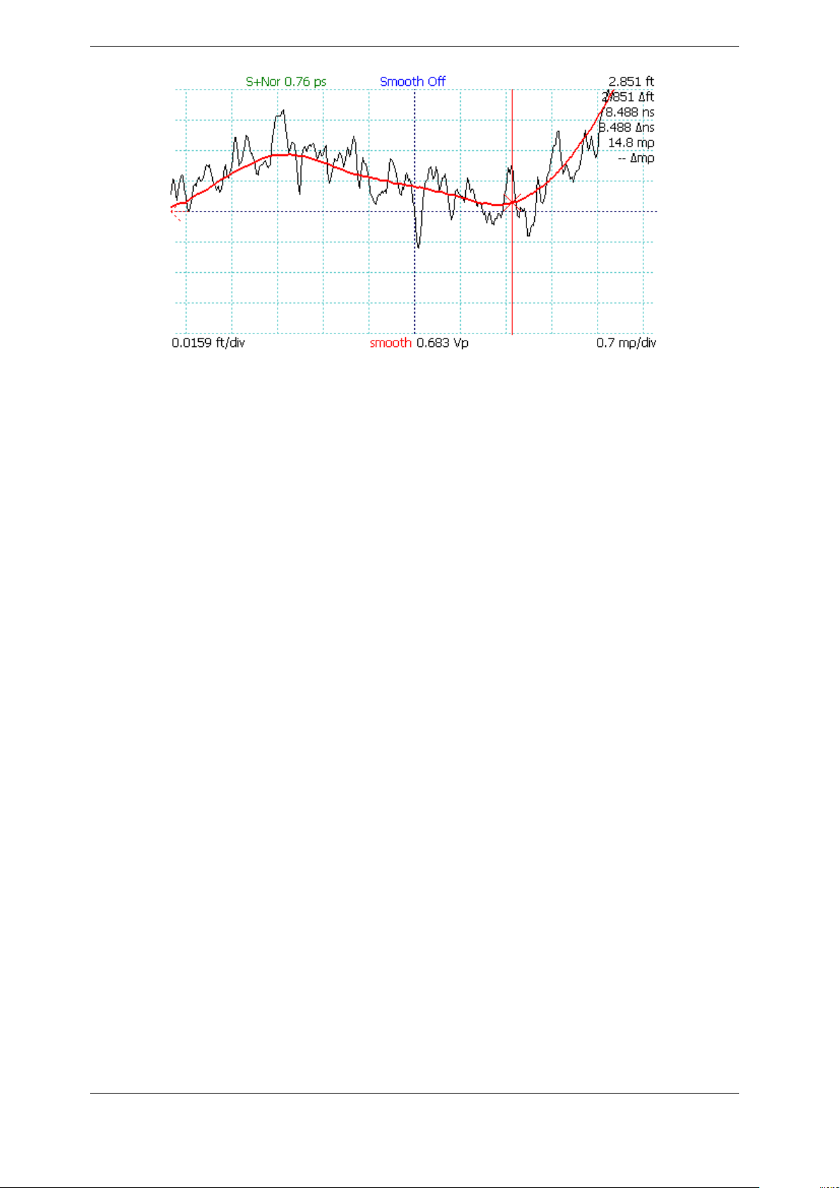
3. Operating Instructions

Figure 3.9. Smoothed vs. unsmoothed traces at very small vertical scales (0.7mρ per
vertical division).

Section 3.11.5). The following TDR trace sample resolution settings are available in the MENU
→ Resolution menu option:

1. Screen: Screen resolution (1 sample/pixel). Fastest trace, adequate for many routine
cable testing tasks. At large horizontal scales, the resolution is low and small faults may
be undetectable, or at least underestimated. This is because there may be too few samples
in the region of the fault for the fault to be reliably identified on the trace. For example, if
a thousand foot cable is displayed on the screen, there is only one measurement about
every two feet.

2. Normal: Sample resolution setting is chosen to match the cable length setting for good
compromise of detail and speed. For SHORT length cable settings, the maximum
resolution is 5.34 ps (less than a millimeter). For MEDIUM length, the maximum
resolution is 17.5 ps (about 2 mm). For LONG length, the maximum resolution is 49.6 ps
(about 5 mm). As you zoom in, the CT100B will adjust resolution.

3. Fixed: Set a sample resolution manually using M-FUNCTION knob; it stays fixed
regardless of screen horizontal scale. Useful for enhancing frequency resolution of S

11

return loss and cable loss traces which may require sampling at resolutions higher than
Normal mode.

Using fine resolution may result in the CT100B buffering. The CT100B will show a green circle
buffering symbol on-screen until buffering is completed.

For larger horizontal scales, the Normal or Fixed sample resolutions provide high resolution
sampling. The trace display at each pixel is a vertical bar that shows the maximum and
minimum values sampled within the pixel. This feature ensures that any detectable TDR

cable fault is displayed at least 1 pixel wide regardless of horizontal scale.

A Normal sample resolution trace of an 800 ft. (250 m) cable is shown in Figure 3.10. In this
case the high resolution sampling of the Normal setting ensures that the small fault from a 50
ohm BNC barrel connector is displayed despite the large horizontal scale. To see this flaw using
only the older Screen sample resolution mode would require the user to “zoom-in” to show the
detail of a short section of cable, and then to manually scroll the length of the cable using the
HORIZONTAL POSITION knob.

CT100B TDR Cable Analyzers Operator’s Manual 31

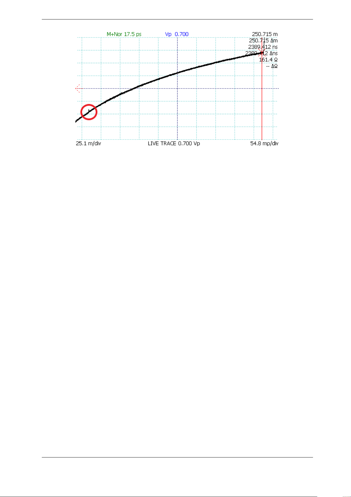
3. Operating Instructions

Figure 3.10. A small fault in a long cable. This fault (red circle) in an approximately 800
ft (250 m) cable is from a 3 cm barrel connector (0.01% of cable length). The sampling
of the Normal sample resolution setting ensures that the cable fault is displayed at this
large horizontal scale (~50 cm/pixel).

3.10.6. Temperature Correction

The CT100B automatically adjusts for changes in ambient temperature. When temperature is
displayed on the screen with Temp Comp toggled on, a message is shown giving the status of
temperature correction. When the CT100B is fully adjusted, the message reads “TC: OK” in
green text.

3.11. Test Procedures

3.11.1. Measure Distance-to-Fault (DTF)

1. Attach the cable to the test port.

2. Set Vp to match the Vp of the attached cable or select an appropriate cable from the cable
type library. See Section 3.11.27 Cable Type Library for instructions on using the cable
type library.

3. Press the AUTOFIT/HELP → AUTOFIT menu option. The CT100B trace is now scaled
to show the entire cable from beginning to end. See Figure 3.11.

4. Note the “bump” in the middle of the cable. This is where two short test cables are
connected with a BNC barrel connector. Position the active cursor on the reflection caused
by this cable fault. Adjusting the vertical scale helps make cable faults more obvious, as
in Figure 3.12 which is at the same horizontal scale as Figure 3.11 but zoomed-in
vertically. By positioning the inactive cursor just before the connector, we can see the
delta value of ~4.4Ω impedance change in the connector vs. the impedance of the cable.

5. Use the HORIZONTAL SCALE and VERTICAL SCALE knobs to further zoom in on the
fault to get a more accurate measurement of Distance-to-Fault (DTF). Position the cursor
at the “toe” or early rising edge of the fault. The distance measurement shown on the
screen for the active cursor is then the Distance-to-Fault. See Figure 3.13.

32 CT100B TDR Cable Analyzers Operator’s Manual

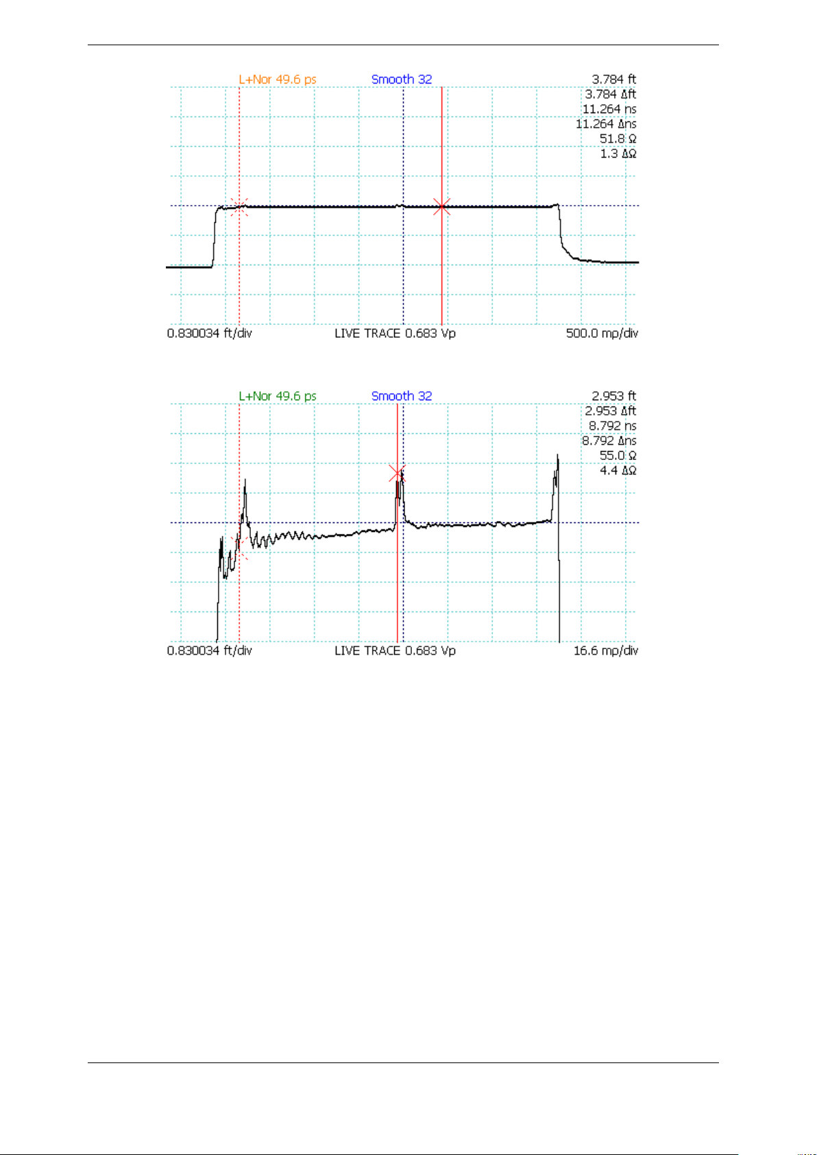
3. Operating Instructions

Figure 3.11. AUTOFIT cable. The cable termination is a short.

Figure 3.12. Vertical scale used to emphasize cable fault.

3.11.2. Relative Distance and DTF Measurements

The CT100B displays the absolute distance from cable start and also the relative distance from
the inactive cursor to the active cursor. Note that Vp must be set accurately for the section of
cable between the cursors for the CT100B to measure relative Distance-to-Fault accurately. The
pulse velocity of any part of the cable that is not between the cursors will not affect the relative
distance measurement. To measure the relative distance between two points in a cable, do the
following:

1. Move the active cursor to the beginning of the section to be measured.

2. Press the CURSOR button to switch cursors.

3. Move the newly active cursor to the end of the section to be measured.

4. The CT100B displays the distance measured between the two cursors as a “∆” value
below the absolute distance measurement. Figure 3.14 is a 3 ft. segment of 50 ohm cable
marked by small impedance “faults” caused by BNC connectors on both ends.

In general for the most accurate relative distance or time measurements between two faults,

CT100B TDR Cable Analyzers Operator’s Manual 33

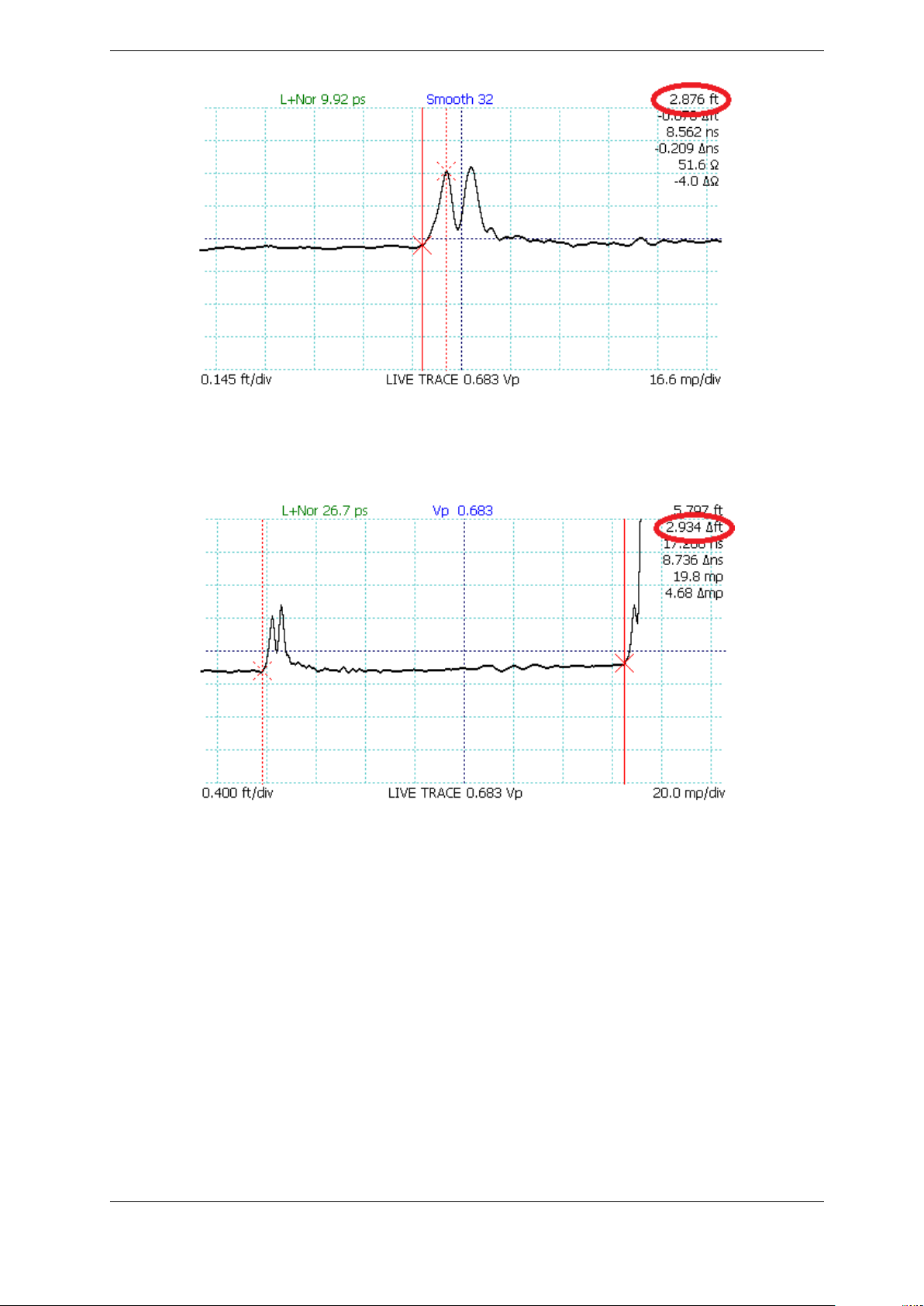
3. Operating Instructions

Figure 3.13. A horizontally zoomed-in view of the cable fault with active (solid) cursor
at the start of the fault (“toe” region) and inactive (dashed) cursor at the peak of the
fault. The DTF measurement is highlighted (red circle).

Figure 3.14. Relative distance measurement between two small impedance “faults”
caused by BNC connectors.

place the cursors on the “toe” region of the faults where the TDR trace is just beginning to rise
above or fall below the cable characteristic impedance.

3.11.3. Multi-Segment Cable DTF Measurements

Cable assemblies are sometimes made up from different types of cables in series, each of which
may be chosen for unique characteristics such as high-temperature operation or radiation
resistance. Such cables frequently have different velocities of propagation (Vp), making
Distance-to-Fault (DTF) measurements difficult. If the average Vp of the assembly or the Vp of
any one cable assembly is used, it will result in inaccurate distance measurements along the
length of the compound cable.

34 CT100B TDR Cable Analyzers Operator’s Manual

3. Operating Instructions

The CT100B includes multi-segment cable measurement capability designed to improve cable
measurement accuracy in the setting of compound, multi-segment cables with differing Vp
values. The CT100B allows the operator to break a TDR trace into cable segments, each of
which can have its own Vp. The distance-to-fault calculated from the compound trace shows
improved accuracy. The following procedure can be used to perform multi-segment cable
measurements:

1. Select MENU → Measurement menu.

2. Select Cable Segments submenu.

3. Place the cursor at the position of the cable segment, marked by a connector impedance
signature or other demarcation, such as physical distance as calculated using known Vp for
a given cable segment.

4. Select Add New Segment.

5. Repeat steps 3 and 4 for each cable segment.

6. Use the Prev Segment and Next Segment selections to select each cable segment and use
the M-FUNC Vp option to set the given segment’s velocity of propagation.

7. The Distance-to-Fault measured by the cursor reflects multi-segment Vp as shown
in Figure 3.15 and Figure 3.16.

Figure 3.15. Multi-segment cable segment with Vp of 0.400 (red circle).

3.11.4. Ohms-at-Cursor Measurements

The CT100B also displays the impedance in ohms (Ω) at the cursor position. A reading before
and after a reflection from a fault shows the impedance mismatch that could cause such a
reflection. Impedance measurements at the first fault in a cable are more accurate than
impedance measurements at more distant faults.

CT100B TDR Cable Analyzers Operator’s Manual 35

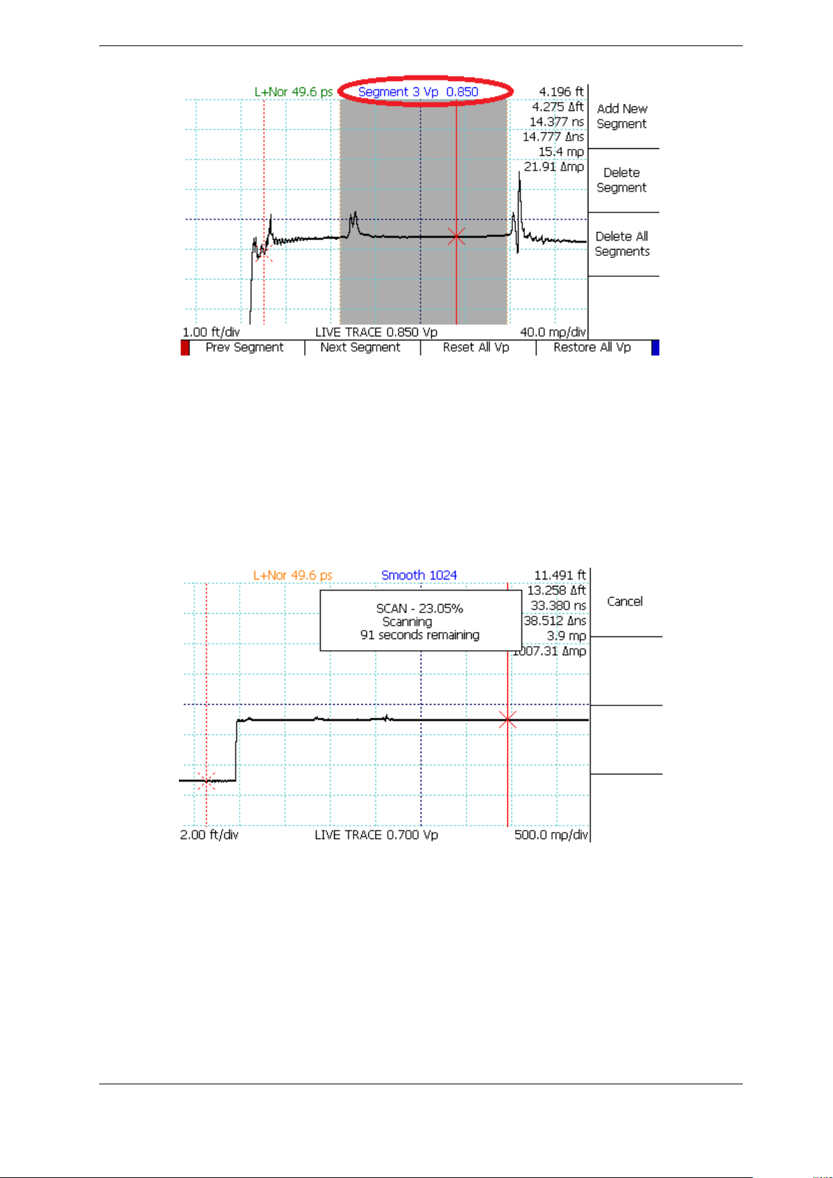
3. Operating Instructions

Figure 3.16. Multi-segment cable segment with Vp of 0.850 (red circle).

3.11.5. Scan a Cable

The CT100B can scan and save a trace into memory. CT100B scans differ from traditional TDR
traces because they can be used to save detail at a much higher resolution than displayed on the
screen. Cable scans can subsequently be reviewed at different levels of detail and compared to
prior scans to identify subtle changes in cable or connector performance. See Figure 3.17 and
Figure 3.18. Scans may also be referred to as traces in this manual.

Figure 3.17. Scan progress display with Cancel button.

Saved scans can appear on the screen in addition to the live trace. Pressing the SELECT
button switches between traces. Vertical position and scale are adjusted for individual traces.
Changing these values for one trace won’t affect other traces.

To scan a cable or cable segment:

1. Press the SCAN button to bring up the Scan menu.

2. Select Snapshot or Cursor.

36 CT100B TDR Cable Analyzers Operator’s Manual

3. Operating Instructions

Figure 3.18. Scan of a portion of a cable (red), zoomed-in vertically to show additional
detail relative to the live trace (black).

3. Choose the Start Scan option from the menu to begin a cable scan.

4. Select the cable scan (see Section 3.11.6 below) and manipulate as needed.

There are two types of scans:

1. Snapshot scan - Capture the live trace as it appears on the screen. This can work well if
using Normal or Fixed resolution mode. If using Screen resolution, the result may be less
detailed.

2. Cursor scan - Captures the entire trace between the two cursors using the current sample
resolution (see Section 3.10.5). This works even if one or both cursors are off-screen when
you begin the scan.

A scanned trace is created using the smoothing factor that is set at the time of the scan.
Because of this, high resolution or highly smoothed scans may take a long time. During a scan,
a menu will appear with a Cancel option. Select Cancel to abort the scan.

3.11.6. Select a Trace

The CT100B always shows one trace on the screen in bold. This is the selected trace. If it is a
live trace, the VERTICAL POSITION and VERTICAL SCALE knobs can be used on the
selected trace, leaving other traces on the screen unchanged. If the selected trace is not a live
trace, you can also use the Save, Rename, and Hide Selected Trace options on the Scan menu
without affecting other on-screen traces. Vertical measurements such as reflection coefficient,
return loss, and impedance are always based off of the selected trace and may disappear if the
cursor scrolls beyond a scanned boundary or is off screen.

Press the SELECT button to change which trace is active. Figure 3.19 shows a screen with
three traces and the LIVE TRACE is selected.

Figure 3.20 shows the same three traces with a saved scan selected. The saved trace has been
moved vertically using the VERTICAL POSITION knob so that it is easier to see.

Figure 3.21 shows the same three traces but now the trace representing the difference between
the two is selected.

CT100B TDR Cable Analyzers Operator’s Manual 37

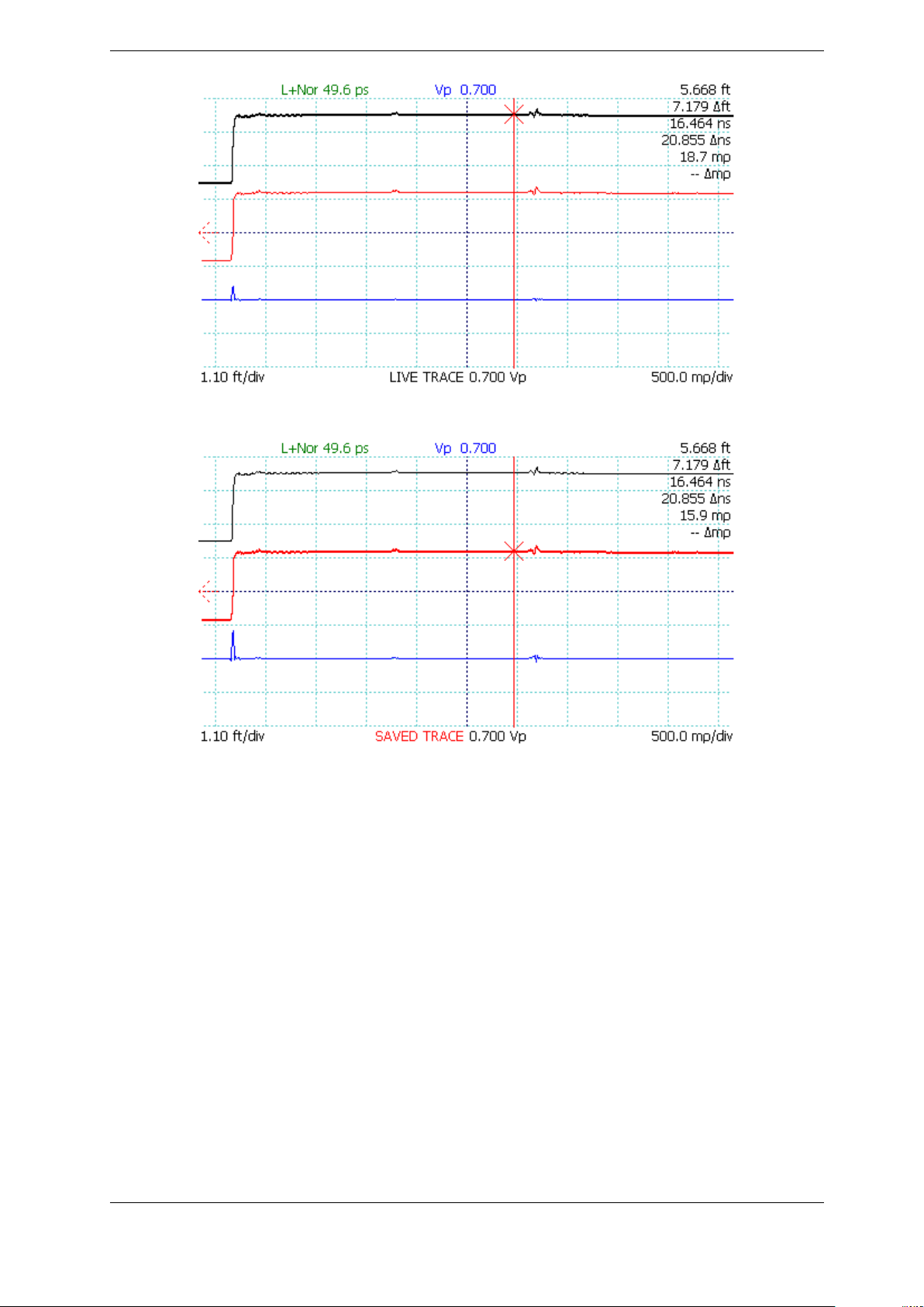
3. Operating Instructions

Figure 3.19. Selecting the live trace.

Figure 3.20. Selecting a scanned trace.

3.11.7. Store a Trace

A scanned trace can be stored for later recall:

1. Press the SCAN button. The Scan menu appears.

2. Press the SELECT button until the scanned trace to be stored is selected.

3. Select the Save option from the menu.

4. The CT100B requires a name for storage and will prompt for one with a dialog box.

5. A dialog menu appears. Press the Show Keyboard menu option to display the on-screen
keyboard or use a USB keyboard.

6. When using the on-screen keyboard use the M-FUNCTION knob to highlight characters.
See Figure 3.22. Review Section 3.7.2 for more information on using the Keyboard menu.
Press the Select Highlighted option to enter the highlighted letter into the name.

7. Press the OK option from the menu when finished.

The trace is now stored, and can be recalled later by name under FILE → Cable Scan Records.
Other trace types, such as difference traces, derivative traces, and frequency domain traces (such

38 CT100B TDR Cable Analyzers Operator’s Manual

Figure 3.21. Selecting a difference trace.

3. Operating Instructions

as FFTs) can also be stored with the same process.

3.11.8. Load a Trace (Cable Records)

A stored trace can be loaded back to the screen:

1. Press the FILE button. The File menu appears.

2. Select the Cable Scan Records option. A scrolling dialog box (see 3.7.2.1) appears for the
selection of a stored trace.

3. Use the M-FUNCTION knob to highlight the trace you wish to load.

4. Press the Select menu option to load the trace.

The stored trace now appears on the screen. It can be selected and manipulated the same as
any scanned trace. See Figure 3.23 in which the loaded trace (red, top) has been translated
slightly upward using the VERTICAL POSITION knob in order to improve visualization. Some
stored traces, such as FFT traces, require some re-calculation to fully load. This calculation is
done automatically, but it may take several seconds.

CT100B TDR Cable Analyzers Operator’s Manual 39

3. Operating Instructions

Figure 3.22. Using the on-screen keyboard. Choose Hide Keyboard when finished. Then
choose OK to save the trace with the name you entered.

Figure 3.23. Loading a trace.

40 CT100B TDR Cable Analyzers Operator’s Manual

3. Operating Instructions

3.11.9. Storing, Transferring, and Deleting Traces

The CT100B has a large storage space, capable of holding thousands of trace scans. However,
with continued use, CT100B storage will eventually fill up. Periodically, an effort should be
made to clear stored traces from the device and free up storage space.

3.11.9.1. Transferring Traces

The CT100B ships with an installation DVD for the CT Viewer™ (Version 2) software for
Windows. Using either a USB or an Ethernet connection, the CT100B can transfer stored scans
to CT Viewer 2. These scans are then stored in the Windows computer for later retrieval,
review, email, and analysis. See Section 4: CT Viewer™ and/or the CT Viewer™ 2 Quick User
Guide for details on transferring traces to a computer using CT Viewer 2.

3.11.9.1.1. Export Trace to File Traces can also be exported to a USB drive for storage, or to
transfer to CT Viewer 2 or to another CT100B. To export one or more traces to USB:

1. Insert a USB drive into the front panel of the CT100B.

2. Press the FILE button, and then press the Cable Scan Records menu option.

3. Mark specific traces for transfer using the Toggle Selected option or select them all with
the Mark All option.

4. Press the Export → USB menu option. A message should appear after a short time
confirming that the traces were transferred.

3.11.9.1.2. Export Trace to CSV The active trace can be exported to a .csv file on an
attached thumb drive. To do this:

1. Select the desired trace to export using the SELECT button.

2. Press the FILE button to open the file menu.

3. Press the Export → CSV menu option. A dialog box will appear displaying the name of
the file to be used.

4. Change the file name to the desired name using a USB keyboard or the on-screen
keyboard by pressing the Keyboard menu option.

5. Press the OK menu option. A message should appear after a short time that confirms the
trace was exported.

3.11.9.2. Deleting Traces

Once scans are backed up to a computer, they can be deleted from the CT100B either through
the CT Viewer 2 software or directly as follows:

1. Press the FILE button to open the File menu.

2. Select Cable Scan Records. A scroll dialog appears, showing all saved trace scans.

3. Mark specific traces for deletion using the Toggle Selected option or select them all with
the Mark All option.

4. Select the Delete option. You will have to confirm the deletion.

CT100B TDR Cable Analyzers Operator’s Manual 41

3. Operating Instructions

3.11.10. Mask Testing

The CT100B is capable of performing mask testing on the currently displayed live TDR trace.
The mask creates an area around the scanned trace that functions as a test limit for the live
TDR trace. Any point of the trace that extends into the masked area will cause the background
to turn red. This can be used for creating acceptance criteria for cable segments and connectors.
See Figure 3.24 and Figure 3.25 for examples of traces passing and failing a mask test.

Figure 3.24. A trace that passes the mask test

Figure 3.25. A trace that fails the mask test

To create a Mask, use the following procedure:

1. Create a cable scan or load a scan from memory that will be used to generate a mask.

2. Select File → Masks menu.

3. With the desired cable scan selected, select Create Mask from Trace.

4. The CT100B will generate a mask using the selected cable scan and display it on the
screen. If the live TDR trace fits within the mask, it will appear with a green background.

42 CT100B TDR Cable Analyzers Operator’s Manual

3. Operating Instructions

5. Use Change Vertical Margin and Change Horizontal Margin to adjust the mask
boundaries around the trace.

3.11.10.1. Storing a Mask

The CT100B is capable of storing thousands of masks. To do this:

1. With a mask already displayed select File → Masks menu.

2. Select Masks. This will open a dialog for saving, exporting, loading, and deleting masks.

3. Select Add New.

4. The CT100B requires a name for storage and will prompt for one with a dialog box.

5. A dialog menu appears. Press the Keyboard menu option to display the on-screen
keyboard, or use a USB keyboard.

6. When using the on-screen keyboard, use the M-FUNCTION knob to highlight characters.
See Figure 3.22 for more information on using the Keyboard menu. Press the Select
Highlighted option to enter the highlighted letter into the name. Press Hide Keyboard to
accept the name.

7. Press the OK menu option when finished.

The mask is now stored and can be recalled later by name under FILE → Masks → Masks.

3.11.10.2. Loading a Mask

To load a saved mask from storage, use the following process:

1. Press the FILE button. The File menu appears.

2. Press the Masks option to enter into the Masks menu.

3. Press the Masks option again to enter into the mask storage dialog.

4. Use the M-FUNCTION knob to highlight the mask you wish to load.

5. Press the Select menu option to load the mask.

The stored mask will now appear on-screen after a brief loading time.

3.11.10.3. Exporting/Importing a Mask

Masks can be exported to and imported from a USB drive in order to replicate mask testing on
multiple CT100Bs. Exporting can be done by:

1. Press the FILE button. The File menu appears.

2. Press the Masks option to enter into the Masks menu.

3. Select Masks option again. A scroll dialog appears, showing all saved masks.

4. Use the M-FUNCTION knob to highlight the trace you wish to export.

5. Press the Export → USB option.

6. The mask will be copied to the USB drive.

To import a mask to the CT100B, do the following:

1. Press the FILE button. The File menu appears.

2. Press the Masks option to enter into the Masks menu.

3. Select Masks option again. A scroll dialog appears, showing all saved masks.

4. Use the M-FUNCTION knob to highlight BROWSE USB.

5. Press the Select option. This will navigate to the attached USB drive.

CT100B TDR Cable Analyzers Operator’s Manual 43

3. Operating Instructions

6. Use the M-FUNCTION knob to highlight the mask to be imported.

7. Press the Import → Internal option.

8. The mask will be copied to internal storage of the CT100B.

3.11.10.4. Deleting a Mask

Once masks are backed up to a computer, they can be deleted from the CT100B as follows:

1. Press the FILE button to open the File menu.

2. Press the Masks option to enter into the Masks menu.

3. Select Masks option again. A scroll dialog appears, showing all saved masks.

4. Mark specific masks for deletion using the Toggle Selected option or select them all with
the Mark All option.

5. Select the Delete option. You will have to confirm the deletion.

3.11.11. Envelope Plot (Transient/Intermittent Fault Detection)

Cable system troubleshooting frequently involves detecting and localizing transient or
intermittent faults, such as a twisted pair cable with frayed insulation that briefly shorts its
conductors when mechanically disturbed, or a coaxial connector that reflects an open when
shaken. The CT100B’s Envelope Plot mode simplifies characterization of these types of
intermittent faults. To create an Envelope Plot, use the following procedure:

1. Position the TDR trace such that the area of interest is located on the screen at a
satisfactory horizontal and vertical scale. Resolution from previous measurement will be
preserved.

2. Select MENU →Measurement menu.

3. Select Envelope Plot submenu.

4. Select Envelope Plot Off to turn Envelope Plot mode on.

5. Use the Fill Mode On/Off option to toggle between Fill Mode and Probability Density
display mode.

6. The CT100B can monitor a trace for extended periods of time with appropriate power
management settings are enabled.

7. Sometimes manipulation of the cable and/or connectors of interest during Envelope Plot
monitoring will provoke an intermittent TDR fault.

Fill Mode fills in an area plot between the maximum and minimum impedance values. This is
useful to highlight the location of the fault because the fault typically creates an “arrow” that
points to the location of the fault as shown in Figure 3.26.

Probability Density mode shows the underlying TDR traces which can be useful to determine
the fault mechanism and likelihood of occurrence as shown in Figure 3.27. Both modes provide
the range of impedance values at cursor, as shown in Figure 3.28.

44 CT100B TDR Cable Analyzers Operator’s Manual

3. Operating Instructions

Figure 3.26. Envelope Plot with Fill Mode, with the active cursor positioned at the fault
location (red circle). Note that the black lines shown here to emphasize the “virtual
arrow” do not actually appear on the instrument screen.

Figure 3.27. Envelope Plot with Probability Density display.

3.11.12. Difference (Subtraction) Traces

Difference traces are traces calculated from the subtraction of one trace from another trace. A
difference trace can allow the operator to identify subtle changes in cable or connector
performance. It is recommended that for any important cable and connector assembly, the
as-manufactured or known-good configuration of the assembly be scanned and archived on the
CT100B and/or a host PC running CT Viewer 2. Later, these archived traces can be used to
create difference traces from current data to highlight changes in cable assembly impedance. To
create a difference trace, use the following procedure:

1. Press the SCAN button. The Scan menu appears.

2. Press the SELECT button until the first trace of interest is selected.

CT100B TDR Cable Analyzers Operator’s Manual 45

3. Operating Instructions

Figure 3.28. Envelope Plot with Fill Mode, showing the range of impedance values at
the cursor position (51.5–185.4 ohms, red circle)

3. Select the Math option from the Scan menu and choose Set Base. The selected trace will
turn purple and is now a base trace for further Math functions.

4. Press the SELECT button again until the second trace is selected.

5. Select Difference from the Math menu. A new trace is created that displays the difference
between the base trace and the selected trace. See Figure 3.29, which shows 3.43 ohm
excess impedance due to a slightly loosened BNC barrel adapter. The bottom bold trace is
created by subtracting the top (live) trace from the middle (scanned) trace and adjusting
the vertical scale to emphasize trace detail.

Figure 3.29. Difference trace. Live (base trace, purple, top), comparison scan (red,
middle), difference (blue, bottom) traces show 3.43 ohm excess impedance (red circle) on
the live trace due to a loosened BNC connector.

46 CT100B TDR Cable Analyzers Operator’s Manual

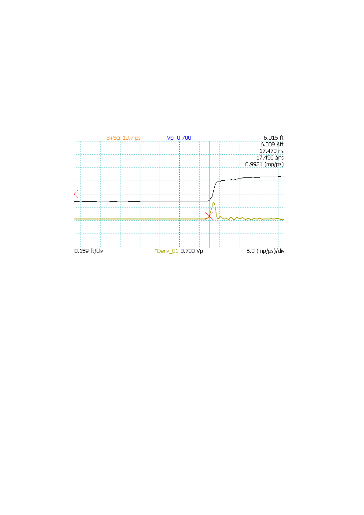
3. Operating Instructions

3.11.13. First Derivative (Slope) Traces

The first derivative trace can be used for two main purposes. First, the first derivative trace can
be used to emulate the trace of a pulse-type TDR. Second, it may be used to remove the
baseline deviation of long or lossy cables caused by resistive loss, so that vertical gain can be
used to emphasize cable faults. To create a first derivative trace, use the following procedure.

1. Press the SCAN button. The Scan menu appears.

2. Press the SELECT button until the trace of interest is selected.

3. Select the Math option from the Scan menu. The Math menu will appear.

4. Select 1st Derivative from the menu.

5. A new trace is created that displays the first derivative of the base trace. See Figure 3.30.

Figure 3.30. First-derivative trace (yellow, bottom).

3.11.14. Second and Higher Order Derivative Traces

The 1st Derivative function can be applied to First Derivative traces to create second (and
higher) order derivatives.

3.11.15. Vertical Reference (Vert. Ref.) Calibration

Use the vertical reference (Vert. Ref.) system to increase the accuracy of vertical measurements,
including impedance, reflection coefficient, and return loss. The Vert. Ref. feature can be used
with a direct connection, through impedance matching adapters, and using baluns. To calibrate
with the Vert. Ref. feature, use the following procedure:

1. Go to the MENU → Measurement menu.

2. Select the option for Vert. Ref. to display the Vert. Ref. menu.

3. Position the active cursor at the leftmost position where the Vert. Ref. should apply.
Typically, this will be the position where you will apply the open and short attachments in
step five. This position can be changed after the setup.

4. Select the Set Vert. Ref option.

CT100B TDR Cable Analyzers Operator’s Manual 47

3. Operating Instructions

5. A set of terminators, both open and short, are included with the CT100B for calibration
purposes. Attach these terminators to the CT100B when prompted to do so (pn:
CT100-AC-ISS, CT100-AC-ISMM, CT100-AC-IBS, CT100-AC-IBMM).

When the reference measurement is finished, cursor measurements will now appear in blue at
the right hand of the screen, and the notification using vert. ref. will appear underneath.

A green line will appear at the position of the active cursor (see step 3 above). Vertical reference
is applied to all points to the right of the green line. Standard vertical measurements are used
for all points to the left of the green line. The position of this line can be changed with the Vert.
Ref Start menu option.

By default, the impedance value at 0 mρ (millirho) is taken to be 50 Ω. This value can be
changed with the Vert. Ref. Center Imp. menu option. If you are using an impedance matcher
or balun adapter, the center impedance should be changed to the value of impedance of the
adapter. For instance, if you are using a 100 ohm differential pulse splitter balun to measure
differential impedance of twisted pair cable, then the center impedance should be changed to
100 Ω.

The CT100B is now configured for enhanced accuracy impedance measurements across a wide
range of impedances.

The Vert. Ref. On/Off menu option can be used to toggle the vertical reference on and off as
needed for a given cable length setting.

3.11.16. Cable Resistive Loss Correction

The CT100B has a system for correcting for resistive loss (“dribble up”) in cables. This allows
the operator to measure impedance more accurately through long and/or lossy cables.

Under the Measurement menu, there is an item to set ohms per unit length and another item to
toggle the correction on and off. The calculations of this feature assume a linear serial resistance
to an attached cable and no other loss. The procedure for performing resistive cable loss
correction is as follows:

1. Select the MENU → Measurement menu.

2. Select Vertical Correction submenu.

3. Adjust the trace of interest so that it fits on the screen and position the active cursor to
the right of the trace you wish to correct.

4. Select Adjust Ω/ft. (Note: This menu option will show the horizontal units set in MENU
→ Settings → Meas. Settings → Horiz. Units [see Section 3.11.28.1]; i.e., if set to meters,
the menu option will read Adjust Ω/m instead. This is true for all steps in this section.)

5. Select Ω/ft Correct. Off to turn on the correction then press Set Ω/ft Pos. to set the
correction endpoint. The endpoint will appear as a dotted orange vertical line.

6. Rotate the M-FUNCTION knob to change the ohms per unit distance correction setting.
Use the Ω/ft Correct On toggle menu option to turn the correction on or off.

Changing the Ohms/m setting will change the slope of the cable’s trace as the resistive loss is
subtracted, and consequently the impedance readings for all points on the cable’s trace and
beyond. The effect and accuracy of the ohms per unit length value is dependent on the value for
pulse velocity. The effect of resistive cable loss correction on a relatively lossy 72 ohm RG-59
cable is shown in Figure 3.31 and Figure 3.32.

48 CT100B TDR Cable Analyzers Operator’s Manual

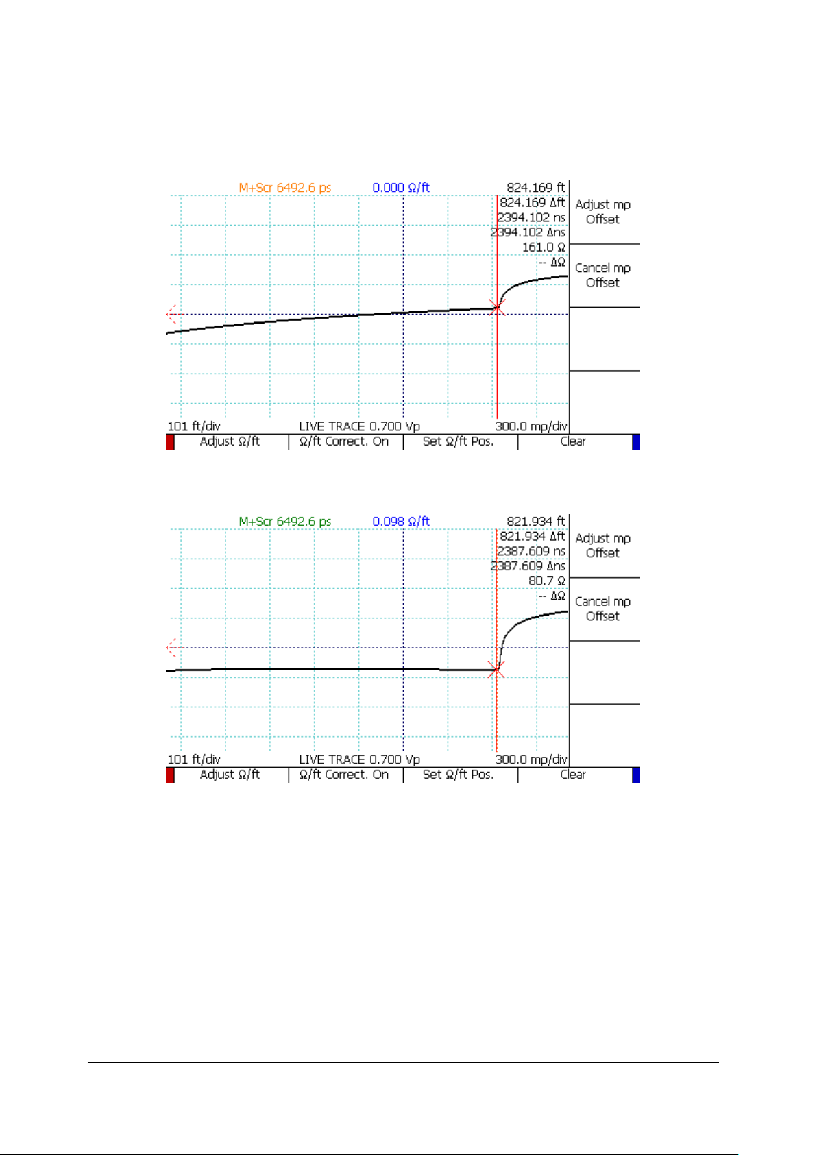
3. Operating Instructions

Use this correction to make more accurate impedance measurements on a length of cable. Since
uniform cables tend to have a characteristic resistive loss per unit length or “dribble up”, one
technique is to adjust the correction until the cable is as flat as possible. Another technique is to
attach a known impedance reference, such as a resistive terminator, to the cable and adjust the
ohms per unit length correction until the measured impedance reads the correct value.

Figure 3.31. Resistive cable loss correction, before. Note that the trace slowly rises.

Figure 3.32. Resistive cable loss correction, after. Note that the trace is nearly

horizontal.

3.11.17. Return Loss (S11) Traces

This feature uses precision open, short, and 50 ohm load (OSL) calibration standard
measurements to correct for systematic errors in the pulsing and sampling electronics, producing
a more accurate S11result on the Device Under Test (DUT). The procedure for creating an S
return loss plot is as follows:

CT100B TDR Cable Analyzers Operator’s Manual 49

11

3. Operating Instructions

1. Prepare the CT100B by setting the trace resolution as desired by going to Resolution →
Fixed and using the M-FUNCTION knob. In general, a resolution of 1-2 ps is adequate to

take advantage of the full bandwidth and frequency resolution of the instrument. Larger
sample intervals can result in lower bandwidth resolution. Smaller sample intervals have
higher frequency resolution but increase sampling time.

2. Use the M-FUNCTION knob to set the smoothing factor to an acceptable level, usually in
the range of 64 to 256 depending on the application. Use higher smoothing factors for
higher bandwidth, lower noise measurements. Higher levels of smoothing improve the
signal to noise ratio (SNR).

3. With the DUT detached, place the leftmost cursor just to the left of the test plane
(the location where the calibration standards will be applied). This is usually just to the
left of the open at the test port or alternatively at the end of the phase stable cable.

4. Attach the DUT to determine the region of interest and place the rightmost cursor
just to the right of the region of interest. This is usually where steady state TDR trace
amplitude has been restored. Detach the DUT to continue calibration.

5. Select the SCAN → Math menu option to open the Math menu.

6. Select SParam & Normalize Tools. This will open the SParam & Normalize Tools menu.

7. Select S11Calibration. After going through an informational message box, the S

11

Calibration menu will appear and the CT100B will ask for the open terminator. Attach
the open terminator and press Scan Open, or alternatively press Use Selected to use the
currently selected trace as the open calibration standard. For the best results when using
type SMA terminators, use a calibrated 3.5 in-lbs (0.4 Nm) torque wrench (pn:
CT100-TL-TORX7) to tighten the test standards as well as the DUT.

8. Follow the same process as instructed to scan or use the selected trace for the short and 50
ohm load calibration standards.

9. The instrument will now ask for the Measured “Device Under Test” (DUT). Press Use
Live to create a live S11trace, Use Selected to create a static S11trace from the currently
selected trace, or Scan Measured to scan the current live TDR trace.

10. Select the S11return loss trace. Use the cursors to measure return loss at cursor and
average return loss between cursors.

Figure 3.33 shows an S11return loss plot and TDR trace for a 2.4 GHz WiFi antenna. The
return loss at 2.4 GHz (2400 MHz) is 20.9 dB.

3.11.18. Return Loss (S11)Options

There are several mathematical transforms to apply to the S11trace and its input traces that
can, in some cases, help reduce irregularities in the final Return Loss plot. These options can be
found under SCAN → Math → SParam & Normalize Tools → S11Options. If the options are
changed when no S11traces exist, then they will be applied to the next S11trace created.
Otherwise, they are applied to the last S11trace that was selected using the SELECT button.
The options can be combined as necessary, and will change the last selected S11trace in real
time.

3.11.18.1. Return Loss (S11) Pre-Filter

The Pre-Filter can reduce aberrations in the S11trace. This can be combined with a Common
Mode Subtraction (CMS) transform on the input traces. To enable or disable these settings, do
the following:

50 CT100B TDR Cable Analyzers Operator’s Manual

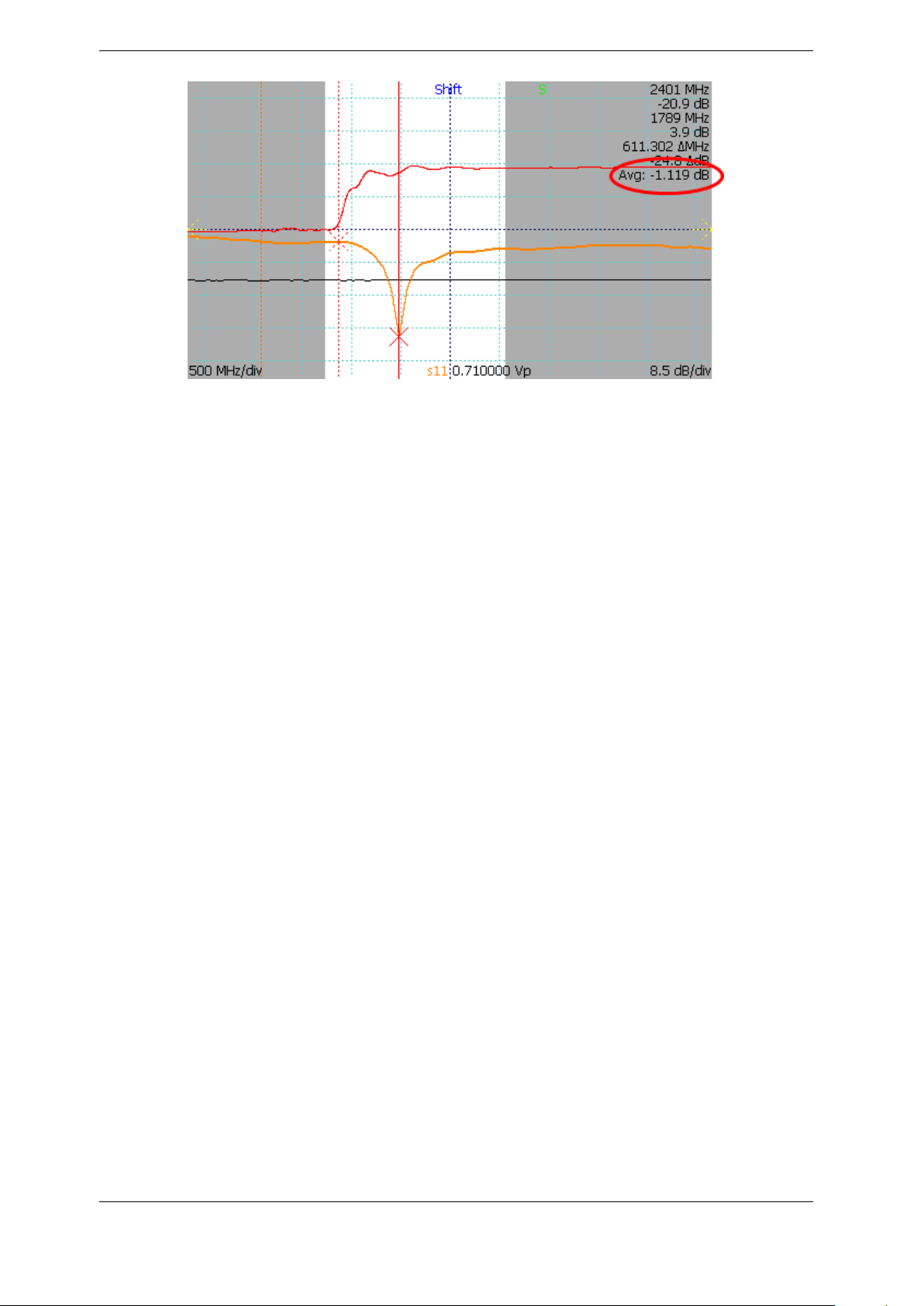
3. Operating Instructions

Figure 3.33. S11return loss plot (orange) and TDR trace (red) of a 2.4 GHz WiFi
antenna. The return loss is calculated on the portion of the TDR trace between the
cursors

1. Create an S11return loss plot using the procedure as described on page 49.

2. Select the S11Options menu, then Pre-Filter Options.

3. Toggle Use this filter to apply filter to the S11trace.

4. Toggle Common Mode Subtraction (CMS) to apply this option to the S11trace.

5. Filter/CMS Offset Ratio is the start of the Aberration Filter and/or Common Mode
Subtraction relative to the S11trace test plane. The default value is 1.66, and is ideal in
most cases.

6. Frequency (MHz) is the aberration filter frequency. The default value is 200, and is ideal in
most cases.

7. Press OK to change the settings to those set above. The S11trace will update using the
new settings.

3.11.18.2. Return Loss (S11) Post-Filter

The Post-Filter can reduce excess noise in the S11trace. To enable or disable the setting, do the
following:

1. Create an S11return loss plot using the procedure as described on page 49.

2. Select the S11Options menu, then Post-Filter Options.

3. Toggle Use this filter to apply filter to the S11trace.

4. Frequency (MHz) is the noise filter frequency. The default value is 20,000 (20 GHz), and is
ideal in most cases.

5. Toggle Apply Hanning to apply a Hanning Window to the filter.

6. Press OK to change the settings to those set above. The S11trace will update, although it
might not look visually different, depending on the settings.

3.11.18.3. Return Loss (S11) Phase Correction

Phase Corrections reduces phase error oscillation in the S11trace. To enable or disable the
setting, do the following:

CT100B TDR Cable Analyzers Operator’s Manual 51

3. Operating Instructions

1. Create an S11return loss plot using the procedure as described on page 49.

2. Select the S11Options menu, then Phase Corr. Off menu option to toggle to Phase Corr.
On. The S11trace will update, although it might not look visually different, depending on
the settings.

Phase Correction typically works best when started at the S11trace test plane. To choose a
different starting point:

3 Use the SELECT button to select a TDR trace, position the active cursor where desired,

then press Phase Corr. Start. The Phase Correction starting point will go to the active
cursor position, and the S11trace will update, although it might not look visually
different, depending on the settings.

3.11.18.4. Time-Domain Gating, or Return Loss (S11) Between Cursors

The CT100B is able to use time-domain gating (also called time windowing) to de-embed
features in the time-domain trace for analysis in the frequency domain using the S11Between
Cursors feature. All other time-domain features are excluded from the analysis so that only the
feature of interest is analyzed. To perform Between Cursors return loss, use the following
procedure:

1. Create an S11return loss plot using the procedure as described on page 49.

2. Use the SELECT button to select a TDR trace.

3. Position the cursors around the feature of interest (e.g., a fault or connector).

4. Select the S11Options menu, then Between Cursors Off menu option to toggle the S

11

Between Cursors feature on. The S11trace may change to reflect just the features in the
highlighted time-domain cursor interval.

5. Pressing the Between Cursors On menu option again will change it to Between Cursors
Hold, which will keep the time-domain region fixed while moving the time-domain cursors.
Otherwise, you may select the S11trace to make frequency-domain measurements using
the cursors without changing the time-domain windowing.

See Figure 3.34 through Figure 3.36 for an example of an S11return loss plot between cursors.
The cursors bracket an SMA barrel adapter between two 3 ft. segments of coaxial cable. The
S11return loss plot shows average 34.46 dB loss across the connector. A loosened connector
shows average loss of 26.7 dB across the connector, compatible with 7.7 dB excess return loss
compared with the tightened connector.

3.11.18.5. Return Loss (S11) Calibration Standards

Many precision Open, Short, and Load standards have unique offset and coefficient values
included with them. By correcting the S11trace with these values, the error introduced by these
terminators can be reduced. To apply or change these standards, do the following:

1. Create an S11return loss plot using the procedure as described on page 49.

2. Select the S11Options menu, then Calibration Standards.

3. Toggle Use Calibration Kit Standards to apply offsets and coefficients to the S11trace.

4. Set the Characteristic Impedance in Ohms. This is defaulted to 50.

5. Enter the offsets and coefficient values provided with the Open-Short-Load Calibration
Standards. If none are provided, or they are unknown, set these values to 0.

52 CT100B TDR Cable Analyzers Operator’s Manual

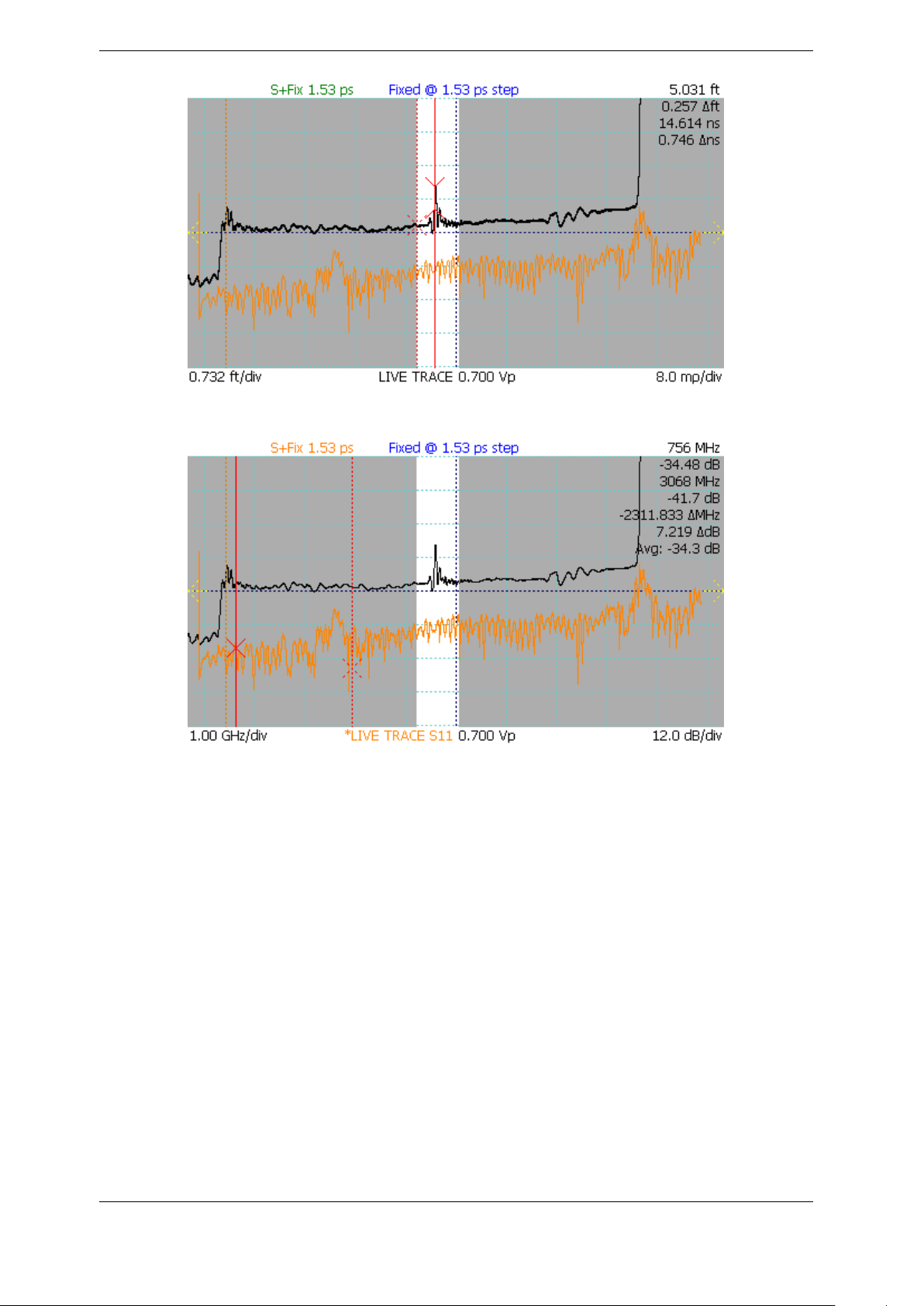
3. Operating Instructions

Figure 3.34. S11between cursors bracketing an SMA barrel adapter on the TDR trace.

Figure 3.35. S11between cursors with tightened connector showing average return loss

of -34.46 dB from 756 MHz to 3 GHz.

6. Toggle Restore Defaults to disregard the values set in the table, and to use those loaded
from the CT100B internal storage. If this is checked when OK is pressed, all former values
will be overwritten.

7. Press OK to change the settings to those set above. The S11trace will update, although it
might not look visually different, depending on the settings.

3.11.18.6. Return Loss (S11) Other S11Options

Additional miscellaneous options can be found under SCAN → Math → SParam & Normalize
Tools → S11Options → Other S11Options, and then toggle the options desired.

• OSL Bases Visible: If not checked, the Open, Short, and Load traces will be hidden after
the S11trace is created. This is to help reduce the visual clutter of the display.

• Align Base Traces: If checked, and if the input traces to the S11trace all include the
internal cabling, the input traces are aligned to the common first rise of the internal cable.

CT100B TDR Cable Analyzers Operator’s Manual 53

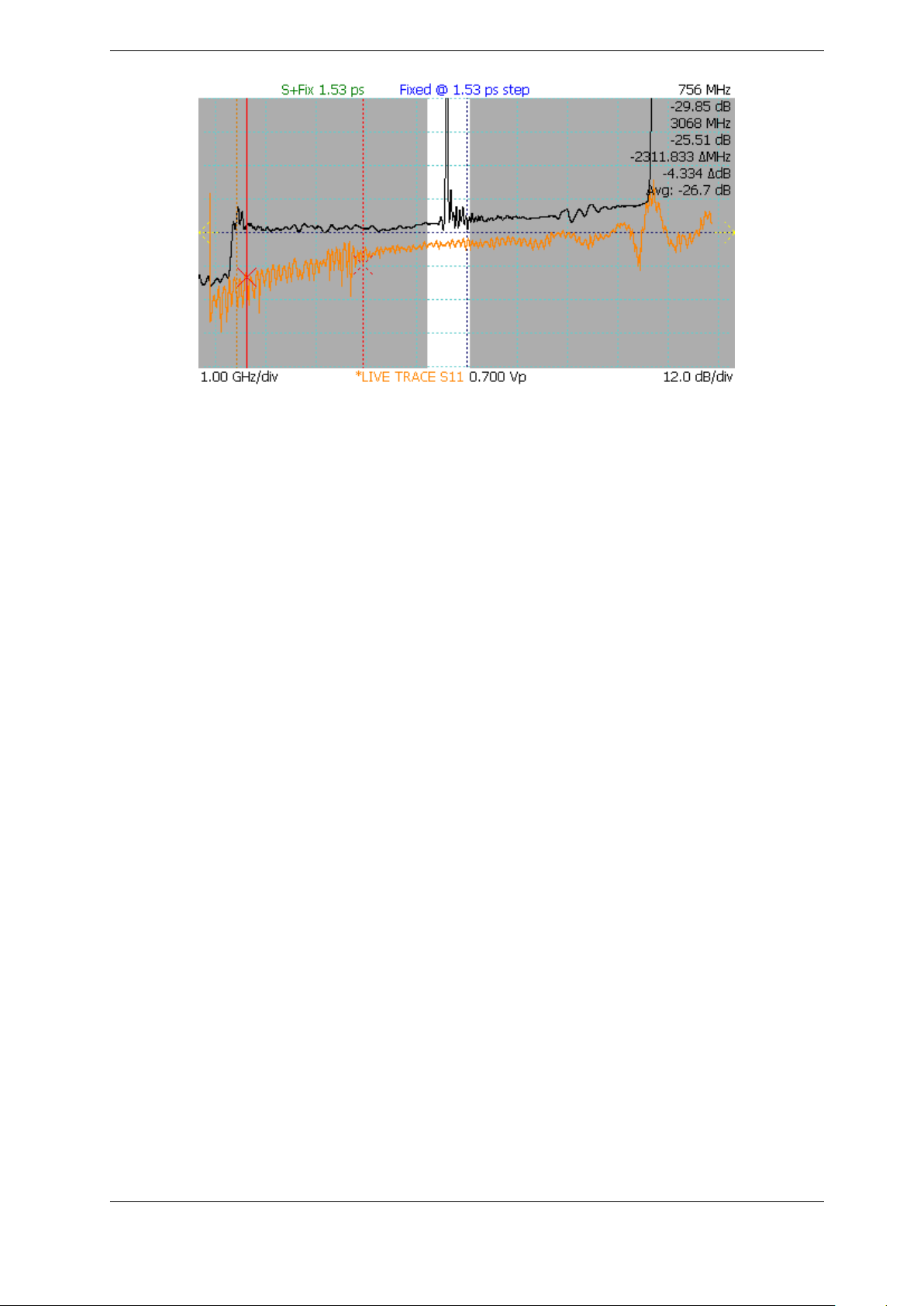
3. Operating Instructions

Figure 3.36. S11between cursors with loosened connector showing average return loss of

-26.7 dB from 756 MHz to 3 GHz (7.7 dB excess return loss compared with the tightened
connector in Figure 3.35).

3.11.19. Improving S-Parameter Measurements

Note that testing short microwave cables directly from the test port may cause unacceptable
noise due to the presence of secondary reflections in the TDR trace. In general, this shows up as
excessive spectral noise. In this case, time windowing can be used to restore measurement
accuracy:

1. Attach a 2 ft. phase stable cable to the test port of the instrument.

2. Place the leftmost cursor just to the left of the end of the phase stable cable.

3. Identify the start of the multiple reflections on the cable under test and exclude this region
with the cursors (see Figure 3.37).

4. Perform SParam calibration as described in Section 3.11.17.

The time-windowed trace will have substantially reduced noise due to exclusion of the secondary
reflections.

3.11.20. Smith Charts

The Smith chart is a useful graphical tool for plotting reflection coefficients and complex
impedance values and can be used to simplify impedance matching. For a very brief
introduction to Smith charts see Section 5.12. The CT100B allows the operator to display
S-parameter return loss and cable loss traces on a Smith chart. To create a Smith chart, use the
following procedure:

1. Create an S11return loss plot using the procedure as described on page 49.

2. With the S11trace selected, adjust the cursors to minimum and maximum frequency
desired on the Smith chart.

3. Go to SParam Tools and select the Smith Chart option to toggle Smith chart display.

4. Use the HORIZONTAL POSITION knob to move the cursor along the complex
impedance curve.

54 CT100B TDR Cable Analyzers Operator’s Manual

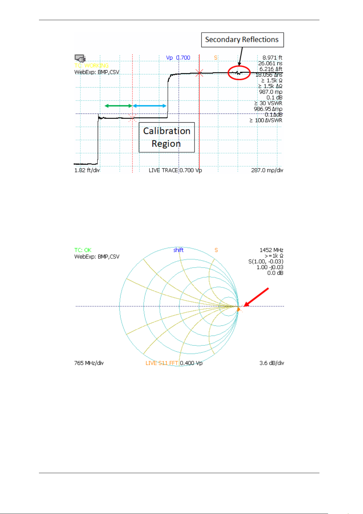
3. Operating Instructions

Figure 3.37. Using a phase stable cable to improve S-parameter measurements on short
microwave cables. Use the phase stable cable (green arrow) and position the rightmost
cursor to the left of the secondary reflections (red circle) occurring after the open or short
at the end of cable under test (blue arrow) so that they are excluded.

Figures 3.38 - 3.41 show Smith chart representations of an open, short, resistive 50 ohm load,
and a reactive 200 ohm load.

Figure 3.38. Smith chart representation of open fault (red arrow).

CT100B TDR Cable Analyzers Operator’s Manual 55

3. Operating Instructions

Figure 3.39. Smith chart representation of short fault (red arrow).

Figure 3.40. Smith chart representation of a 50 ohm resistive load (red arrow).

3.11.21. Normalized TDR Traces

This process creates a normalized TDR trace based on a calibrated S11return loss trace. A
normalized TDR trace appears as another trace in the region of S11calibration. The normalized
trace should be cleaner than the Measured DUT trace, with fewer aberrations. The normalized
trace also has an adjustable rise time to help the operator determine what effect a particular
cable fault will have on signals with differing rise times. The following procedure creates a
normalized TDR trace:

1. Create an S11return loss plot using the procedure as described on page 49.

2. From the SParam & Normalize Tools menu, select Apply Normalization.

3. Select Normalize Pulse Rise Time and use the M-FUNCTION knob to select a suitable
rise time for the cable system as applicable. Note that selecting a rise significantly shorter
than the native rise time of the TDR instrument will result in a degraded trace.

4. Note that the S11Options, such as the Between Cursors On/Off setting is used by the
TDR normalization process. If Between Cursors mode is turned on, the normalized trace

56 CT100B TDR Cable Analyzers Operator’s Manual

3. Operating Instructions

Figure 3.41. Smith chart of reactive 200 ohm load showing effect of reactive impedance
at higher frequencies. Cursor (red arrow) shows impedance value calculated at DC (0
MHz).

information will be taken from the time-windowed S11trace.

Figure 3.42 shows a normalized TDR trace (blue) with a short fault in a 50 ohm cable. The
normalized trace shows reduced aberrations and more accurate relative reflection coefficient and
impedance after the fault compared with the live TDR trace.

Figure 3.42. Normalized trace (blue, bottom) showing short fault in a 50 ohm cable.

3.11.22. Vertical Units

The CT100B is able to change vertical units of the live TDR trace so that it is displayed in
units of reflection coefficient (millirho), impedance (ohms) or voltage standing wave ratio
(VSWR). To change vertical units, use the following procedure:

1. Select MENU → Measurement menu.

CT100B TDR Cable Analyzers Operator’s Manual 57

3. Operating Instructions

2. Select Vert. Units to toggle through the different options.

Example trace with impedance (ohms) as the vertical unit is shown in Figure 3.43. Note that
the vertical scale is in ohms and the open fault at the end of the cable on the red (Impedance)
trace shows nonlinear relationship between the reflection coefficient and the impedance
described in Section 5.6.

Figure 3.43. TDR trace with impedance vertical units (red, top) demonstrating vertical
scale in ohms and emphasis of the open fault at the end of the cable. The black trace
uses reflection coefficient (millirho) as its vertical units.

3.11.23. Layer Peeling (Dynamic Deconvolution) Traces

The CT100B includes the capability to perform layer peeling/dynamic deconvolution. This is a
useful technique for improving impedance accuracy by removing the effects of multiple
reflections caused by impedance discontinuities along the length of the cable. In general, any
impedance discontinuity creates both forward (transmission) and backward (reflection) waves. If
reflected off other impedance discontinuities, these reflected waves will constructively or
destructively interfere along the length of the TDR trace, leading to impedance measurement
errors. The CT100B Layer Peeling feature iteratively extracts the underlying reflection
coefficients as described in Section 5.14. For a more detailed description of layer peeling, see
Section 5.14. To create a layer peeling trace, use the following procedure:

1. Position the TDR trace on the screen so that the region of interest is visible with a portion
of 50 ohm cable visible at the left hand of the screen (use the CT100B’s internal 50 ohm
cable if needed).

2. Use the HORIZONTAL POSITION knob to place the active cursor on the 50 ohm cable
at the left side of the screen. The location of this cursor will define the start of the left
side of the layer peeling trace.

3. Select Math menu.

4. Select Layer Peeling menu option.

An example of a layer peeling trace is shown in Figure 3.44. This figure depicts a multi-segment
cable of varying impedance (50-125-75-63 ohms) with an open fault at the end. The corrected
impedance of the final segment is within 2-3 ohms of the actual value, which represents an ~80%
reduction in impedance error when compared with the uncorrected live TDR trace.

58 CT100B TDR Cable Analyzers Operator’s Manual

3. Operating Instructions

Figure 3.44. Example layer peeling trace (yellow, bottom) versus live TDR trace (white,
top). The layer peeled trace reduces the impedance error in the final cable segment
(green arrows) by ~80%.

3.11.24. Fast Fourier Transform (FFT) Traces

The CT100B can calculate FFT frequency domain information from live and scanned TDR
traces. FFT traces can be used to show the frequency domain content of a trace or portion of a
trace between cursors, and comparisons of FFT traces can be used to demonstrate differences
and/or changes in frequency content, such as between different types of connectors or cable
faults. To create an FFT trace, use the following procedure:

1. Select the live trace with the SELECT button.

2. Use the CURSOR button and the HORIZONTAL POSITION knob to set the boundaries
for the FFT with a cursor at either end.

3. Press the SCAN button, and then select Math → FFT Tools.

4. Select Apply FFT. The CT100B will now take a high resolution scan of the live trace
between the cursors, and then convert the scan into an FFT plot.

FFT traces can be stored, reloaded, and transferred to CT Viewer 2 just like normal scanned
traces.

3.11.25. Web Export

The CT100B is able to export raw data and images in real time over Ethernet. To enable this
feature, follow this procedure:

1. Select MENU → Settings → Network Settings.

2. Toggle Web Export to On or Fast.

3. Using a web browser, navigate to one of the following address:

a) Live trace data is found at http://<<IP_addr>>/www/trace.csv and is stored as

comma seperated values.

b) Selected trace data is stored in as a CSV at

http://<<IP_addr>>/www/selected.csv.

c) A screenshot of the CT100B is available as a bitmap at

http://<IP_addr>/www/screenshot.bmp.

CT100B TDR Cable Analyzers Operator’s Manual 59

3. Operating Instructions

3.11.26. Remote Control

Using the accompanying CT Viewer™ 2 software, the CT100B can be operated by remote
control. The remote control system allows the operator to manipulate traces and store movies of
traces over time. Remote control only functions over Ethernet connections. It does not work
when the CT100B is connected by USB only.

Refer to Section 4.1.3 Send Saved Traces Using Ethernet and Section 4.1.4 Using Remote
Control for instructions on connecting CT Viewer 2 to the CT100B and enabling remote control.
Please consult the CT Viewer 2 Quick User Guide for more information about using remote
control and manipulating a remote TDR trace.

3.11.27. Cable Type Library

The CT100B has a library of common cable types and associated velocities of propagation. Vp
for these cable types can be loaded from the library. The user can add custom cable types to the
CT100B as well. The user-added cable types are stored and accessed separately from the
standard cable types.

3.11.27.1. Load a Cable Type’s Vp

To load a cable type, follow this procedure:

1. Press the FILE button. The File menu appears.

2. Select Reference Cable Types or Custom Cable Types from the menu. An interface appears
that allows you to scroll through the cable types with the M-FUNCTION knob.

3. Highlight the desired cable type and press Select. Vp is now set to the value for that cable
type.

3.11.27.2. Custom Cable Types

The CT100B is able to save custom cable types. Use the following procedure to save a custom
cable type:

1. Press the FILE button. The File menu appears.

2. Select the Custom Cable Types menu option to access user-editable cable types with menu
options Add New and Select.

3. When Add New is chosen, a window appears for entering a cable type name, a Vp for
velocity of propagation, and an expected characteristic impedance for the cable. When the
window first appears, Vp will be set to the current system Vp, while impedance defaults to
50 ohms.

3.11.28. Other Measurement Settings

3.11.28.1. Change Horizontal Units

Horizontal distance measurements can be displayed in meters, inches, feet, yards, or
centimeters.

1. Select the MENU → Settings → Meas. Settings menu.

60 CT100B TDR Cable Analyzers Operator’s Manual

3. Operating Instructions

2. Select the Horiz. Units menu item to switch between the different unit options.

All measurements and all traces are immediately updated to reflect the unit change. Time in
nanoseconds (ns) is displayed separately.

3.11.28.2. Fine Vp Control

By default, the CT100B displays three decimal places for Vp; however, the CT100B can display
six decimal places for Vp when very precise distance measurements are needed.

1. Select the MENU → Settings → Meas. Settings menu.

2. Select Vp 3 Sig Figs from the menu to toggle the option to Vp 6 Sig Figs. The CT100B
will display six decimal places for the Vp readout on the screen when Vp 6 Sig Figs is
shown on the menu.

3. When the CT100B is in Vp 6 Sig Figs mode, a new function, Fine Adj. Vp, is added to
the M-FUNC button. When the M-FUNC button is set to Fine Adj. Vp, turning the
M-FUNCTION knob will change the Vp value by the 6th significant digit. The Vp value
can be changed by thousandths by setting the M-FUNC button to the Coarse Adj. Vp
function.

3.11.28.3. Relative Reflection Coefficient (RRC) Method

The CT100B measures the relative reflection coefficient between cursors. When the two cursors
of the CT100B are positioned on either side of a change in impedance, this measurement is the
reflection coefficient for that change. The relative reflection coefficient is displayed on-screen
with a prefix of ∆mρ. To view the relative reflection coefficient values, go to MENU → Settings
→ Display and make sure Rho is toggled on. By default, the value is displayed in Classic mode,
displaying the true reflection coefficient relative to the signal at the input of the reflection. The
CT100B can also measure in 1502C mode, which displays a reflection coefficient relative to the
signal at the input of the cable.

1. Select the MENU → Settings → Meas. Settings menu.

2. Select RRC Classic Mode from the menu. This will toggle the CT100B between the
Classic RRC calculation and the 1502C calculation as displayed on the screen.

3.11.29. User Configurations

The CT100B allows the user to save individually named instrument configurations. A saved
configuration stores the values of all instrument settings that can influence trace measurements.
A configuration can be called up by its name, restoring all settings to the values saved in that
configuration.

User Configurations can reduce operator error when configuring the TDR to make important
measurements. For this reason it is recommended that User Configurations be used when
setting up the CT100B for important measurements, such as quality-control checks on a cable
manufacturing line.

If a configuration named DEFAULT is saved, that configuration will be initially employed
whenever the CT100B is powered on.

CT100B TDR Cable Analyzers Operator’s Manual 61

3. Operating Instructions

3.11.29.1. Save Configurations

1. Press the FILE button. The File menu appears.

2. Select the Config Entries menu item. The User Configurations library is displayed.

3. Select Add New to add a new User Configuration. The CT100B will prompt you for a
configuration name and will save the current instrument configuration when you press OK.
See Navigating Dialog Boxes on page 15 for information on using the Keyboard menu.

3.11.29.2. Load Configurations

1. Press the FILE button. The File menu appears.

2. Select the Config Entries menu item. The User Configurations library is displayed.

3. Scroll through saved configurations with the M-FUNCTION knob.

4. Press Select to load the highlighted configuration. All settings saved in that configuration
are automatically restored. Measurements and traces are updated to reflect the new Vp,
cursor position, and other applicable settings.

3.11.30. Take a Screenshot

To save a screenshot, first insert a USB drive into the CT100B. Then hold down the SELECT
button and press the M-FUNC button to trigger the screenshot.

A dialog will appear asking for a name for the screenshot. When OK is pressed on the dialog,
the screenshot will be saved to the root directory of the USB drive.

Alternatively, pressing the Print Screen button on an attached USB keyboard will also trigger a
screenshot.

62 CT100B TDR Cable Analyzers Operator’s Manual

4. CT Viewer

The CT Viewer™ 2 host computer software allows users of the MOHR CT100B TDR Cable
Analyzer to transfer, view, and manipulate cable scans that have been saved on their
instruments. This software package allows the user to select scans from a stored database that
can contain thousands of scans and compare, subtract, or find the first derivative of any of the
traces.

This software package will also allow the user to create reports and print plots that can be
imported into Microsoft® Word® or other word processing or report creation software to create
files of traces suitable for transfer to others and to load trace files created by others.

This section covers how to transfer saved TDR traces to CT Viewer 2. For more detailed
information on installing and using CT Viewer 2, please see the CT Viewer 2 Quick User
Guide.

4.1. Sending Saved Traces to a Computer

When a scanned trace is saved to the CT100B, it can be sent to a computer that has CT Viewer
2 installed.

4.1.1. Send Saved Traces with a Thumb Drive

1. Insert a USB drive into a USB port on the front of the CT100B. Wait until the USB drive
icon appears on screen.

2. Press the FILE button to bring up the File menu.

3. Choose the Cable Scan Records menu option. A window listing all of the traces saved to
the CT100B appears.

4. Use the M-FUNCTION knob to select a trace to send to the USB drive. Alternatively use
Toggle Selected and Mark All to select multiple or all traces, respectively.

5. Choose Export → USB from the menu. The select trace(s) will now be written to the USB
drive.

6. Remove the USB drive for the CT100B and insert the drive into a USB port on the
computer.

7. Start CT Viewer 2, and from the File menu in CT Viewer 2, select Open Trace.

8. Select the scan file name(s) of interest from the thumb drive. The trace(s) will be loaded
into CT Viewer 2 and shown on the screen.

CT100B TDR Cable Analyzers Operator’s Manual 63

4. CT Viewer

4.1.2. Send Saved Traces over USB

4.1.2.1. Setup USB Drivers on the Host Computer

The USB drivers need to be set up only once for each computer. The USB drivers for the
CT100B should have been installed with CT Viewer 2. It is possible to skip this step during the
installation. If the drivers aren’t installed, Windows will inform the user when the CT100B is
connected over USB.

4.1.2.2. Send the Traces

1. Start CT Viewer 2 and connect the computer to the CT100B with a standard USB type A
to USB type B cable. Connect to the USB type B port on the back of the CT100B.

2. Go to the File menu in CT Viewer 2 and select Open Tester. A screen will appear that
will show the serial number of the connected CT100B and a list of all traces saved on the
CT100B.

3. Select a trace to transfer by clicking with the mouse. Select multiple traces by holding
down the Shift or Ctrl key while clicking with the mouse.

4. Select the Transfer To button to send the traces to CT Viewer 2. The traces will also be
shown on the screen.

4.1.3. Send Saved Traces Using Ethernet

4.1.3.1. Setup Ethernet

In order to send traces over Ethernet to a computer, both the computer and the CT100B need
to be setup for the network. Depending on the how your network is configured, the default
settings for the CT100B may work. If not, have your network administrator setup the network
settings for the CT100B and the computer.

The CT100B network settings are located at MENU → Settings → Network Settings. The
CT100B can get a configuration through DHCP, or it can be setup with Static Network Settings
(see Network Settings in Table 3.4: MENU Button and Menus).

4.1.3.2. Connect to CT Viewer 2 – First Steps

1. Make sure both the computer and the CT100B are plugged into the network. The
CT100B Ethernet plug is found on the back of the CT100B. The light on the CT100B
Ethernet port should illuminate.

2. Start CT Viewer 2 on the computer.

3. On the CT100B, navigate to MENU → Connect to CT Viewer. See Figure 4.1. The Find
CT Viewer menu button will scan the local network looking for a PC running the CT
Viewer 2 program.

4. Or you can use the Manual Connect option to reconnect to a server you have used in the
past or one that is not on your local network. See Figure 4.2.

64 CT100B TDR Cable Analyzers Operator’s Manual

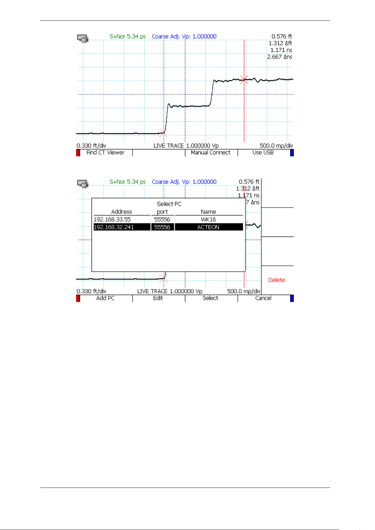
Figure 4.1. Options under the Connect to CT Viewer menu.

4. CT Viewer

Figure 4.2. Selecting Manual Connect in the Connect to CT Viewer menu will bring up a
server menu.

4.1.3.3. Manual Connection the First Time

1. From the server menu, Select Add PC . A window with various server settings appears.

2. Use the M-FUNCTION knob to move up and down in the window. Use the on-screen
keyboard or a USB keyboard to enter values. In PC Name, enter a user friendly name for
the computer.

3. In PC Address, enter either a network name or an IP address for the computer.

4. Do not change the default port number.

5. Press OK to save the server entry, then press Select to connect. If the connection is
successful, a message will appear in CT Viewer 2.

4.1.3.4. Connecting After the First Time

1. Navigate to the MENU → Connect to CT Viewer → Manual Connect menu. A window
showing all the stored server connections will appear.

CT100B TDR Cable Analyzers Operator’s Manual 65

4. CT Viewer

2. Use the M-FUNCTION knob to highlight the connection for the computer.

3. Press Select. The CT100B will try to connect to the server. On success, a message appears
in CT Viewer 2.

4.1.3.5. After Connecting

1. Go to the File menu in CT Viewer 2 and select Open Tester. A screen then appears that
shows the serial number of the connected CT100B and a list of all traces saved on the
CT100B.

2. Select a trace to transfer by clicking with the mouse. Select multiple traces by holding
down the Shift or Ctrl key while clicking with the mouse.

3. Select the Transfer To button to send the traces to CT Viewer 2. A dialog box will
appear. Verify that the destination folder is correct and choose Start Transfer. The traces
will appear on the screen.

4.1.4. Using Remote Control

After the CT100B has connected to a computer over Ethernet using the steps in Section 4.1.3,
go to CT Viewer 2 and select Remote Control → Enable Remote Control.

Once Remote Control has been established, a new, live trace will appear in CT Viewer 2. This
trace will be identical to the trace on the CT100B screen. It can be moved around or scaled just
like any other trace in CT Viewer 2.

Normally the CT100B screen goes blank during remote control. To turn on the CT100B screen
at the same time as Remote Control, select Remote Control → Assistant Mode in CT Viewer

2.

4.1.5. Record and Playback Real-Time TDR Trace Movies

CT Viewer 2 can record a real-time movie of the TDR trace, useful for detecting and
characterizing transient/intermittent faults. To record a real-time movie of the CT100B trace,
connect to the CT100B as described in the previous section, and then select Remote Control →

Record to Movie File. You will be prompted to enter a filename for the recording. Select Remote
Control → Stop to stop the recording. To view the individual TDR traces saved in the movie,

go to File → Open Other Files and locate and select the desired movie (CTM) file. Use the >
and < keys to step forward and backward in the file. The time stamp of the trace is shown as
part of the trace label.

66 CT100B TDR Cable Analyzers Operator’s Manual

5. TDR Measurement Theory

The purpose of this section is to familiarize the operator with the basic theory of time-domain
reflectometry measurement theory in preparation for using the CT100B instrument.

5.1. Time-Domain Reflectometry (TDR)

TDR is a form of closed-circuit radar in which a transient test signal is injected into a
device-under-test (DUT) such as a cable, and reflected voltages are measured over time to
construct a TDR waveform or “trace”. Assuming a transmission line such as a cable with
uniform geometry, the test signal propagates with a characteristic velocity such that the time
can be related to distance. The changes in reflected voltage in a TDR trace with respect to time
correspond to distance from the test port to impedance changes.

Cable or connector faults are regions where the measured reflection coefficient and associated
impedance are outside of manufactured specification. Cable faults are almost always broadband
with preferential attenuation of higher frequencies, and indicate one or more of the following
problems:

1. Change in the geometry of the conductors with respect to one another,

2. Change in the dielectric properties of the insulator, and/or

3. Partial or complete interruption in one or both of the signal conductors.

Cable faults are important because they degrade signal quality. Short or open faults completely
disrupt signal transmission. In many ways such “hard” faults are helpful because they are easy
to diagnose. However, more subtle partial or “soft” faults cause portions of the signal energy to
be reflected and/or delayed, contributing to noise. This can show up as reduced bandwidth in
microwave/RF cable systems and increased bit error rates in digital cable systems.

Multiple small faults that are individually insignificant with respect to noise may contribute in
an additive fashion to exceed the overall “noise budget” of the cable assembly. Because TDR
typically measures the transmission line with sensitivity well below the bit error threshold of
most communications systems, it is useful to find these “insignificant” faults and deviations
from manufactured specification that may contribute to signal integrity problems.

5.2. Reflection Coefficients

The amplitude of reflected voltage at a particular location in a TDR waveform is determined by
the reflection coefficient at that location. The CT100B displays reflection coefficient on the right
hand side of the screen with units of millirho (mρ) and relative reflection coefficient with prefix
of ∆mρ.

CT100B TDR Cable Analyzers Operator’s Manual 67

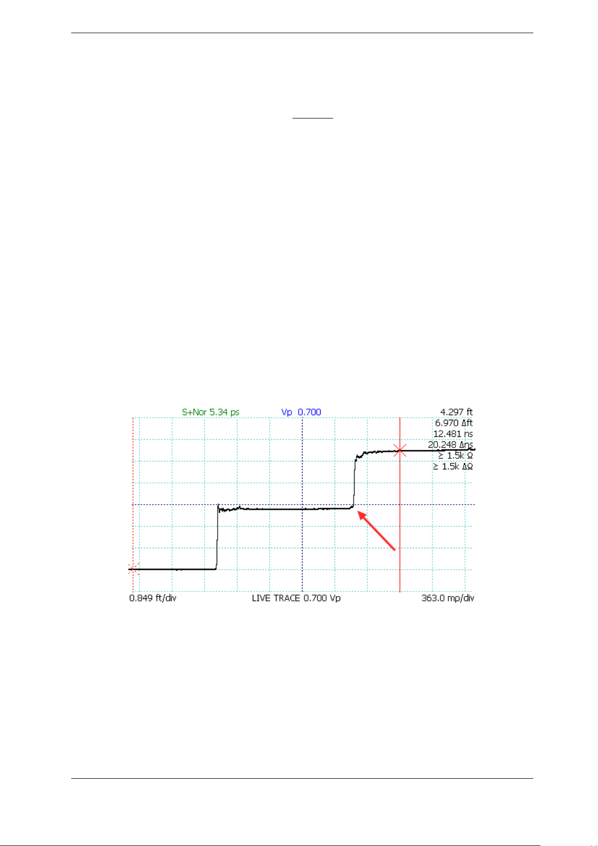
5. TDR Measurement Theory

The reflection coefficient is the ratio of the amplitude of the reflected portion of the test signal
to the amplitude of the incident test signal. The reflection coefficient (Gamma, Γ) is related to
the impedance change (Z) at a given point in a cable according to:

Γ =

ZL− Z
ZL+ Z

S

S

Where ZLis the impedance of the load (e.g., the device under test [DUT]) and ZSis the source
impedance of the TDR, typically 50 ohms but potentially other values if an impedance matching
adapter is being used. The reflection coefficient uses units of rho (ρ) or millirho (mρ).

Note that the reflection coefficient (Γ) is a complex variable with unique amplitude and phase
for each frequency. However, when measuring reflection coefficient directly from a TDR trace,
the measured value is the average reflection coefficient over all frequencies in the incident and
reflected test signal.

The CT100B is also able to measure and display frequency-domain complex reflection coefficient
values in the context of S11return loss and cable loss plots such as those produced with Vector
Network Analyzer (VNA) and Frequency Domain Reflectometer (FDR) equipment. This is
discussed further on page 76.

5.3. Common Types of TDR Cable Faults

Open faults appear as a pulse upward in the TDR trace (Figure 5.1) because the fault reflects
all of the incident step energy in-phase with the test signal.

Figure 5.1. An open cable fault shows an upward step edge at the location of the fault.

Short faults appear as a pulse downward in the TDR trace because the fault reflects all of the
incident step energy 180◦out-of-phase with the test signal (Figure 5.2).

Short or open faults measured through long lengths of cable (hundreds of feet) will show long,
shallow reflections on the TDR trace because the cable preferentially attenuates higher
frequencies in the test signal, degrading the rise or fall time of the reflected fault. Figure 5.3
demonstrates a TDR trace with an open fault at the end of an 824 ft. RG-6 coaxial cable with

68 CT100B TDR Cable Analyzers Operator’s Manual

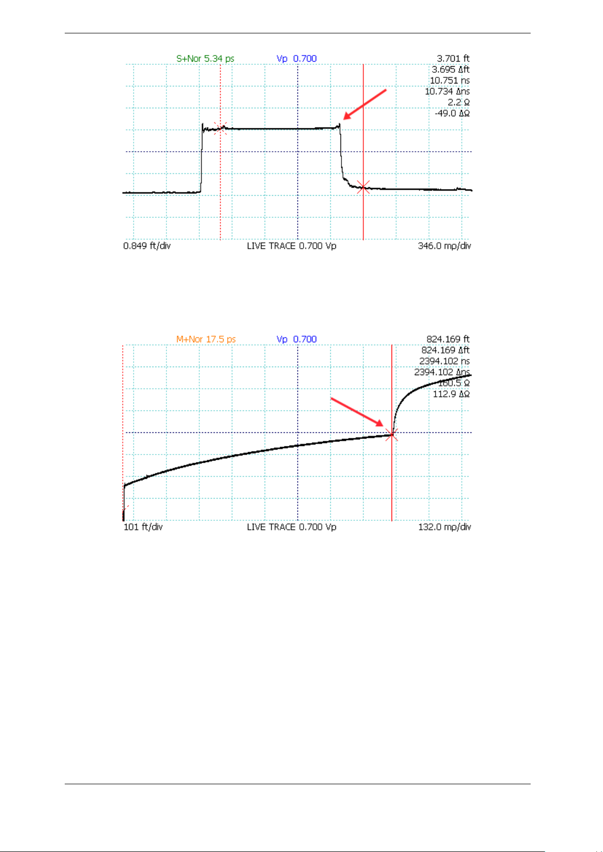
5. TDR Measurement Theory

Figure 5.2. A short cable fault shows a downward step edge at the location of the fault.

long, shallow reflected rise caused by cable attenuation of high frequency components of the step
pulse.

Figure 5.3. An open cable fault at 824 ft.

Faults with reactive components such as capacitance and inductance appear as either dips below
or bumps above the characteristic impedance of the cable, depending on whether they are in
series with the conductor or represent a fault to ground.

Normal connectors will show up as an impedance discontinuity simulating a small fault.
Depending on the type and quality of the connectors, the expected impedance variation will
differ, as shown in Figure 5.4 and Figure 5.5 for SMA and BNC type connections. Connector
damage and corrosion can change the impedance profile of a connector over time, typically
increasing the excess impedance of the connector. Periodic surveillance with TDR can be used
to confirm connector performance.

Soft/partial faults can appear anywhere along the cable’s length. Any fault has the potential to
reduce the incident pulse strength for subsequent cable faults and may change the apparent

CT100B TDR Cable Analyzers Operator’s Manual 69

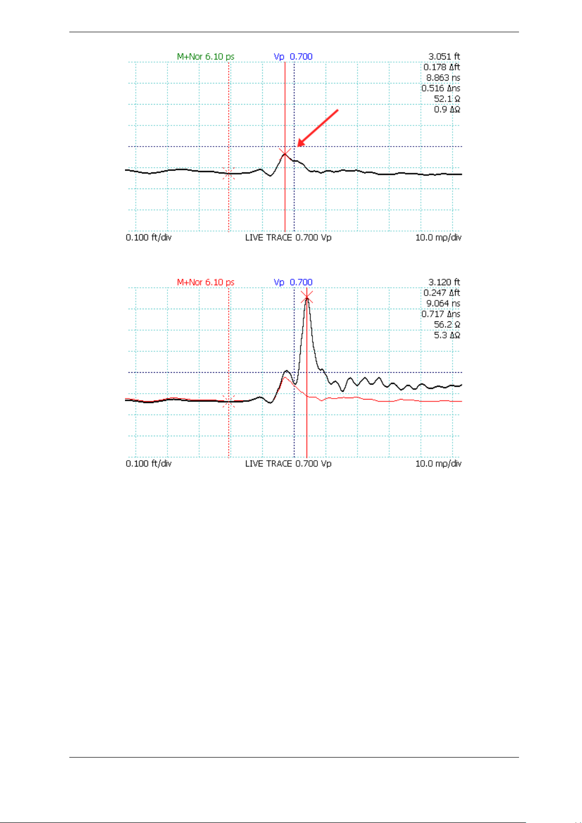
5. TDR Measurement Theory

Figure 5.4. Normal SMA female barrel interconnect measuring 52.1 ohms.

Figure 5.5. Comparison of typical SMA (red trace, bottom) and BNC (black trace, top)

coaxial cable interconnects.

velocity of propagation. The accuracy of the Distance-to-Fault measurement of a fault that
appears beyond another fault is reduced.

5.4. Velocity of Propagation (VoP, Vp)

As mentioned in previous sections, a transmission line, such as a cable, has uniform geometry
with a characteristic signal propagation velocity. This velocity of propagation (Vp, VoP, or VP),
sometimes also called the velocity factor (VF) or wave propagation speed, is the measure of the
velocity of an electrical signal within a cable expressed as a fraction of the speed of light in a
vacuum. With the CT100B, Vp can be set between 0.250000 and 1.000000.

Nominal Vp values for most types of cable can be found in the manufacturer’s data sheet, and
Appendix E: Vpof Common Cables contains nominal values for a variety of commonly used cable
types. These values can be a good start for basic cable Distance-to-Fault measurements, however

70 CT100B TDR Cable Analyzers Operator’s Manual

5. TDR Measurement Theory

it is important to be aware that Vp values for a given cable type may vary from manufacturer to
manufacturer and from one manufacturing lot to the next even from the same manufacturer. In
addition, cable aging due to temperature, radiation, or other environmental parameters may
alter the original characteristic velocity of propagation for a given cable. For this reason, if
accuracy is particularly important for a particular cable Distance-to-Fault measurement, it is
generally a good idea to establish a known Vp for a sample of the specific cable under test.

The velocity of propagation (V p) is related to the dielectric constant (relative permittivity, εr)
of the dielectric medium according to:

V p ≈

Velocity of propagation is also related to the distributed inductance (L) and shunt capacitance
(C) of a lossless transmission line according to:

√

1

ε

r

V p =

1

c√LC

5.5. Distance-to-Fault (DTF) and Cable Length

Once the operator identifies an impedance discontinuity such as a cable fault or open or short
cable termination, the distance to the fault (D) is related to the velocity of propagation (V p),
the speed of light (c), and the measured round-trip time (t) to the fault, according to:

V p · c · t

D =

The product is divided by 2 because the CT100B measures the time for the pulse to travel to
and from the point of interest.

2

5.6. Impedance

As mentioned previously, TDR instruments measure reflection coefficient essentially but must
calculate impedance according to:

Z(t) = −Z

Where Z (t) is the impedance at time t, ZSis the source impedance, and Γ(t) is the reflection
coefficient at t. This is the basis for the CT100B ohms-at-cursor measurements and ZTrace
impedance traces. It is important to note that impedance is nonlinear with respect to reflection
coefficient, as shown in Figure 5.6.

Because TDRs measure reflection coefficient, noise and uncertainty on a TDR trace is in units of
millirho, not ohms. Given a fixed amount of uncertainty in reflection coefficient, the
corresponding impedance uncertainty will be low at impedances less than the TDR source
impedance (typically 50 ohms) and increasingly larger and nonlinear for impedance values
greater than the TDR source impedance.

The CT100B factory calibration provides typical vertical accuracy of approximately 0.1 ohm
near 50 ohms and approximately 10-20 ohms near 1000 ohms for most cable testing applications.

CT100B TDR Cable Analyzers Operator’s Manual 71

Γ(t) + 1

S

Γ(t) −1

5. TDR Measurement Theory

Figure 5.6. Relationship of impedance (ohms) to reflection coefficient (rho) for 50 ohm
source impedance (marked by red circle).

When impedance measurements are very important, accuracy can be improved using Vert. Ref.
(page 47) and normalized TDR traces (page 56).

5.7. Return Loss

Return loss is another way of measuring impedance change in a cable. Return loss is given in
decibels (db) and is always calculated using the relative reflection coefficient. Return loss is
related to the reflection coefficient Γ by the formula:

Return Loss = −20 ·log10|Γ|db

The larger the fraction of energy in the reflected signal, the lower the numerical return loss value,
so that an open or a short that returns 100% of the signal has a return loss of 0 dB. A very low
loss cable will have a large return loss in dB. Likewise a 50 ohm cable terminated with a perfect
50 ohm load will have very large return loss in dB. This relationship is shown in Figure 5.7.

Return loss measured directly from a CT100B TDR trace represents the average return loss over
all frequencies in the step-rise test signal. The CT100B can measure TDR return loss at cursor
and relative return loss between cursors and optionally displays these values at the right hand of
the screen in units of dB, with ∆dB used for the relative return loss measurement.

72 CT100B TDR Cable Analyzers Operator’s Manual

5. TDR Measurement Theory

The CT100B is also able to measure complex frequency-specific S11return loss and cable loss
values such as those produced with Vector Network Analyzer (VNA) and Frequency Domain
Reflectometer (FDR) equipment. This is discussed in further detail on page 76.

Figure 5.7. Relationship of return loss (dB) to reflection coefficient (rho).

5.8. VSWR

Voltage standing wave ratio (VSWR) is a way of displaying reflection coefficient in a nonlinear
way that emphasizes changes in cable impedance. VSWR is the voltage standing wave ratio and
is related to the reflection coefficient Γ according to:

VSWR =

VSWR measures the ratio of the maximum-over-time amplitude of the nodes and anti-nodes of
the standing wave off of a reflection. If there’s no reflection (e.g., 50 ohm termination), VSWR
will be 1. If all energy is reflected (e.g., short or open fault), VSWR goes to infinity. This
relationship is shown in Figure 5.8. VSWR is a unitless, scalar value.

The CT100B displays two different VSWR values at cursor. The first, VSWR, is calculated
from the total reflection relative to the CT100B test port source impedance (50 ohms). The
second, ∆VSWR, is calculated from the reflection between the two cursors. In other words,
VSWR is based on the millirho reflection coefficient, while ∆VSWR is based on the ∆mρ,

1 + |Γ|
1 −|Γ|

CT100B TDR Cable Analyzers Operator’s Manual 73

5. TDR Measurement Theory

Figure 5.8. Relationship of voltage standing wave ratio (VSWR) to reflection coefficient
(rho). VSWR for 50 ohm load is shown by the red circle.

relative reflection coefficient calculation. There are menu options in the Display menu to toggle
the display of VSWR and ∆VSWR.

VSWR can also be selected as the vertical scale for a trace. From the Main menu, go to the
Measurement menu and select Vertical Units.

5.9. Rise Time and Spatial Resolution

Spatial resolution is defined by the ability of the operator to distinguish the presence of two
closely spaced faults on a TDR waveform. An accepted rule of thumb is that the limiting spatial
resolution of a TDR instrument is approximately1⁄2 of the system rise time (10-90%). This is
the time required for the step signal reflected from an open or short termination to transition
from 10% to 90% of the final step amplitude. The estimated spatial resolution R is calculated
by the following equation:

where c is the speed of light and tris the system rise time. If the velocity of propagation Vpis
taken to be 0.66 and the TDR has a 100 ps system rise time, the calculated resolution is ~10
mm.

R

∼

=

1

· c · Vp· t

2

r

Faster system rise times allow a given TDR instrument to more faithfully represent partial cable
faults such as shield nicks or kinks, as shown in Figure 5.9. This figure depicts a simulation of

74 CT100B TDR Cable Analyzers Operator’s Manual

5. TDR Measurement Theory

the difference between a 90 ps rise time TDR and an 800 ps rise time TDR (typical of low-cost
TDR instruments) for characterizing two 1 cm long, 75 ohm faults spaced 1 cm apart on a 50
ohm cable. The 800 ps rise time TDR detects only a single fault and grossly underestimates the
severity of the fault.

Figure 5.9. Simulated comparison of a 90 ps rise time TDR (green) and an 800 ps TDR
(red) with respect to the ability to depict two 1 cm long, 75 ohm faults spaced 1 cm apart
on a 50 ohm cable. Notice how the faster TDR (90 ps) resolves each fault individually.
The blue lines represent a theoretically perfect response.

5.10. Timebase/Cursor/Horizontal Resolution

Timebase, cursor, or horizontal resolution refers to the horizontal spacing of samples along the
TDR trace. In order to faithfully depict the TDR profile of a connector or cable fault, the cursor
resolution should be at least 5 to 10 times higher than the spatial resolution. For the example
just shown in Figure 5.9, it is unlikely that the cursor resolution for the slower rise time
instrument would be adequate to reliably depict the fault in the first case.

Cursor resolution also comes into play when precise length or phase matching of cables is being
carried out, in which the cursor resolution must be sufficient to adequately depict the difference
in length between cables. Typically the cursor resolution should be 10 times higher than the
intended length accuracy.

With respect to frequency-domain measurements, very high cursor resolution ensures adequate
frequency bandwidth because the number of sampled data points in the time domain translates
into frequency resolution in the frequency domain.

CT100B TDR Cable Analyzers Operator’s Manual 75

5. TDR Measurement Theory

5.11. Frequency-Domain Measurements

5.11.1. Scattering Parameters

The scattering parameter or S-parameter approach to describing a device under test (DUT)
assumes that a DUT is a black box network with N ports. The S-parameter matrix contains the
complex reflection and transmission coefficients of the network, describing the amplitude and
phase of reflected and transmitted values from each port in response to excitation of one or
more of the ports.

According to convention, the scattering parameter Sxyrepresents the response of the network in
terms of reflected and/or transmitted voltages at port x in response to excitation of port y. S
and S22are the complex reflection coefficient matrices of port 1 and 2, respectively. S21and S
are the forward and reverse complex voltage gain matrices for port 1 and port 2, respectively.

Considering a 2-port network with incident voltage waves a1= V
waves being b1= V

−

and b2= V

1

−

, the 2-port S-parameter matrix is described by:

2

b

1

b

2

!=

S11S
S21S

12

22

!

!

a

1

a

2

+

and a2= V

1

+

and reflected

2

11

12

Solving for S11gives:

Solving for S21gives:

S11=

S21=

b

1

a

1

b

2

a

1

=

=

−

V

1

+

V

1

−

V

2

+

V

1

Passive networks like cables, splitters, attenuators, and combiners can be considered reciprocal
networks such that S11= S22and S21= S12. One-port measurements can be used to
characterize the return loss (S11/S22) and insertion loss (S21/S12) of a variety of 2-port passive
networks such as cables. This will be discussed in the Cable Loss (S21) section on page 77.

You can measure S-parameters directly in the frequency domain using a VNA instrument and
indirectly in the time domain using a TDR instrument. The TDR instrument performs a discrete
Fourier transform (DFT) operation to decompose a TDR trace into the frequency domain.

When calibration is performed at the test plane using open, short, and 50 ohm load (OSL)
terminations, the CT100B is able to mathematically subtract systemic errors in the pulser and
sampler electronics from the measured trace, improving S-parameter accuracy.

S-parameters measured with TDR instruments are accurate with sufficient dynamic range for
most applications. Figure 5.10 shows a comparison of return loss for a 2.4 GHz WiFi patch
antenna measured using a handheld VNA and CT100HF TDR. The TDR-derived return loss
measurements show good accuracy from DC to approximately 8.3 GHz. Both spectra clearly
show the 2.4 GHz bandpass region expected for a 2.4 GHz WiFi antenna.

76 CT100B TDR Cable Analyzers Operator’s Manual

5. TDR Measurement Theory

Figure 5.10. Comparison of S11return loss of a 2.4 GHz WiFi patch antenna measured
using a handheld VNA (Agilent® FieldFox N9927A, green) and TDR (CT100HF, blue),
showing good agreement from DC to ~8.3 GHz. Note bandpass in the 2.4 GHz region.

5.11.2. Return Loss (S11)

The complex return loss S11is expressed as:

Return Loss RL = −20 · log10|S11|dB

5.11.3. Insertion Loss (S21)

The complex insertion loss S21is expressed as:

Insertion Loss IL = −20 · log10|S21|dB

True 2-port insertion loss measurements require a 2-port instrument; however the cable loss
measurement described below uses the reciprocity feature of passive networks to determine
insertion loss from cables and other suitable 2-port networks using a 1-port test instrument.

5.11.4. Cable Loss (S21)

Cable insertion loss in dB is additive per unit length. Assuming that port 2 of a 2-port DUT
(e.g., a coaxial cable) is terminated with a short (or open) adapter such that all (or nearly all) of
the incident voltage trace is reflected back to the TDR instrument, insertion loss (S21) is half of
the corresponding S11return loss measurement in dB:

Cable Loss CL =

CT100B TDR Cable Analyzers Operator’s Manual 77

RL

2

dB

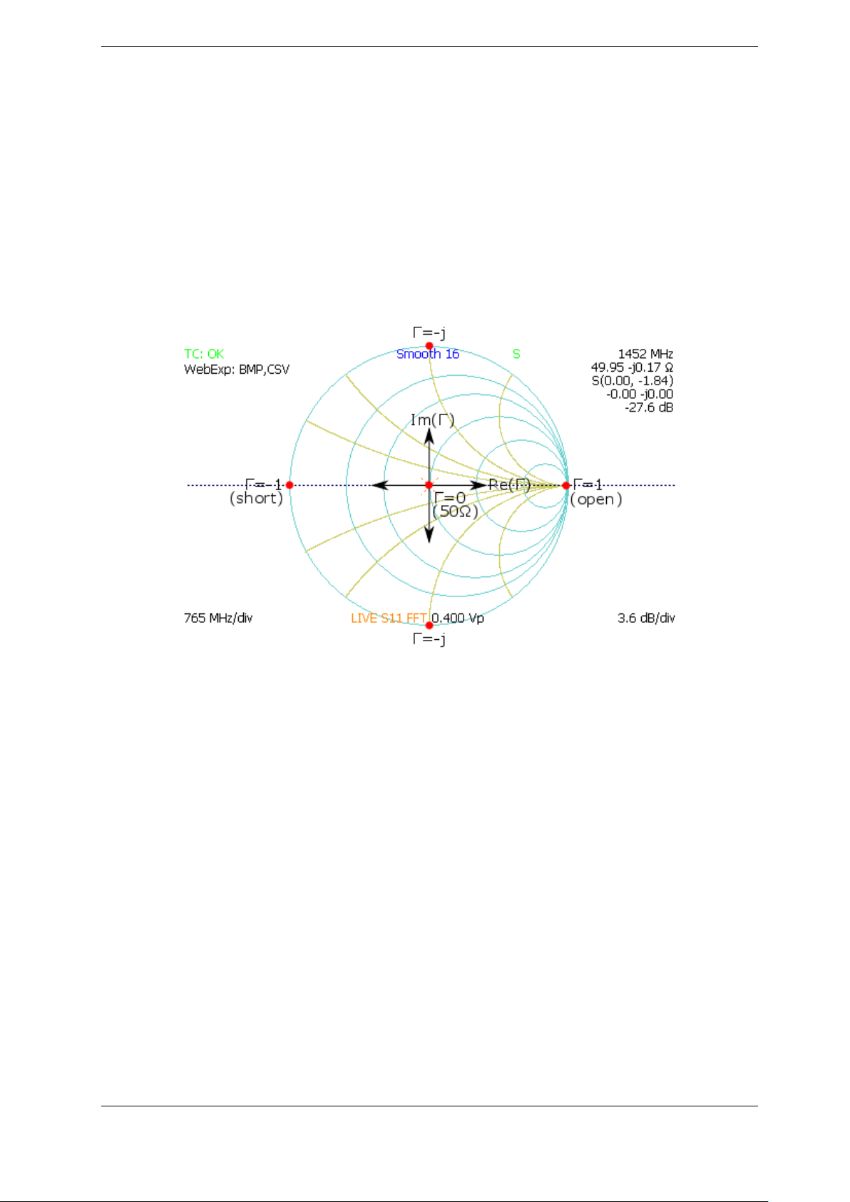
5. TDR Measurement Theory

Again, this relationship is valid if the cable is terminated with a short or open. One drawback to
this technique is that the round-trip insertion loss reduces the length of cable that can be tested
over a given bandwidth relative to a 2-port measurement because the attenuation of the test
signal is doubled. However, for many applications it is adequate.

5.12. Smith Charts

The impedance Smith chart is a useful graphical tool for visualizing complex impedances and
scattering parameters as shown by Figure 5.11. The CT100B includes Smith chart functionality
that can be used to simplify transmission line troubleshooting and impedance matching as
described in Section 3.11.20.

Figure 5.11. Impedance Smith chart relationships.

5.13. Normalized TDR Traces

The S-parameter OSL calibration process mathematically models the TDR pulser-sampler
system as a two-port error network and subtracts systematic pulser-sampler errors from the S
matrix. Convolution of the S11matrix with an idealized Gaussian step or other idealized
excitation signal allows the CT100B to create and display a normalized TDR trace. The
normalized TDR trace has lower aberration and improved impedance accuracy compared with
the original TDR trace.

Although cable fault detection is the most sensitive when using an excitation signal with the
fastest rise time possible, by changing the rise time of the Gaussian step, the importance of a
given cable or connector fault can be estimated at different signal rise times and bandwidths.
For instance if the cable under test is typically used with 1 ns rise time signals, the severity of a
cable fault can be determined by using a 1 ns rise time normalized TDR trace. Localized cable
faults will always appear less severe when examined using slower rise time excitation signals.

11

78 CT100B TDR Cable Analyzers Operator’s Manual

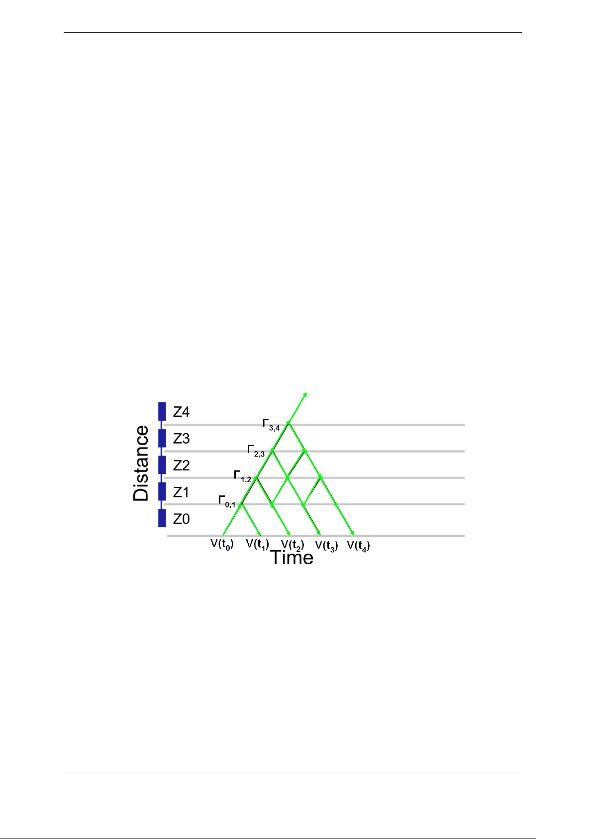
5. TDR Measurement Theory

5.14. Layer Peeling/Dynamic Deconvolution

Layer peeling (or dynamic deconvolution) is a general method to solve the inverse scattering
problem in partially reflective transmission lines such as cables. When applied to TDR traces,
this method attempts to extract the underlying real reflection coefficients and impedance in the
presence of multiple reflections caused by the presence of impedance discontinuities in the cable
assembly under test.

As implemented in the CT100B (see Section 3.11.23), the layer peeling method iteratively
examines the TDR trace at each time step and attempts to correct for forward and backward
signal propagation to extract impedance values at each time step. This is diagrammed in
Figure 5.12 showing measured voltages V (t) taken from the TDR trace and their relationship to
actual reflection coefficients (Γ) at time (t) and impedance values (Zx) at different physical
distances. The diagram shows that for each time step forward in the TDR trace, there are
increasingly complex contributions from forward and backward reflections as they interact with
each new impedance boundary.

For instance, the test signal moving forward from the Z0/Z1impedance boundary is reduced by
the energy reflected by the Z0/Z1boundary. Likewise the Z1/Z2impedance boundary is
“tested” by the original TDR test signal at time t1but also interacts with reflected signals at
every subsequent time point due to internal reflections in the cable. The layer-peeled TDR trace
partially corrects for the presence of these multiple reflections and provides more accurate
impedance values. This effect is most pronounced when there are multiple large impedance
transitions in a cable assembly and at short and open faults.

Figure 5.12. Layer peeling scattering diagram relating measured TDR trace (V [t]) to
actual impedance changes (Z [x]) and their associated actual reflection coefficients
(Γ[x, t]).

CT100B TDR Cable Analyzers Operator’s Manual 79

6. Options and Accessories

6.1. Options

Model CT100B (BNC) – self-grounding BNC test port
Model CT100B (SMA) – stainless-steel SMA test port
Model CT100HF – high-frequency sampler, stainless-steel SMA-type test port

6.2. Accessories

6.2.1. Service accessories (CT100B / CT100HF)

Technical Manual, Printed CT100B-M-TSM-xxx*
Technical Manual, Digital w/ CT Viewer™ 2 Installation CT100-S-CTVTSM-xxx*

* xxx applies to revision number. Accessory part number is incremented per revision.

6.2.2. Standard BNC Accessories – CT100B (BNC)

BNC 50 ohm 36 in. Reference Cable CT100-AC-W536
SMA 50 ohm Terminator CT100-AC-ER50-S
Connector, SMA female to BNC male CT100-AC-ISFBM
BNC Female to Female Adapter CT100-AC-IBFF
BNC Male to Male Adapter CT100-AC-IBMM
BNC Shorting Cap CT100-AC-IBS
24 VDC External Charger/Power Supply CT100-AC-PS
Operator’s Manual, Printed CT100B-M-OM-xxx*
CT Viewer™ 2 Quick User Guide, Printed CT100B-M-CTVM-xxx*
CT Viewer™ 2 Installation DVD, w/ Digital Operators
and CT Viewer™ 2 Manuals CT100-S-CTV2-xxx*
Soft Carrying Case CT100-AC-CS
NIST-Traceable Calibration with Certificate CT100-AC-NISTCC

CT100B TDR Cable Analyzers Operator’s Manual 81

6. Options and Accessories

6.2.3. Standard SMA Accessories – CT100B (SMA), CT100HF

SMA 50 ohm 36 in. Reference Cable CT100-AC-W536-S
SMA 50 ohm Terminator CT100-AC-ER50-S
SMA Male to Male Adapter CT100-AC-ISMM
Connector, SMA female to BNC male CT100-AC-ISFBM
Connector, SMA male to BNC female CT100-AC-ISMBF
Connector, SMA Female Short CT100-AC-ISSF
SMA Shorting Cap CT100-AC-ISS
24 VDC External Power Supply CT100-AC-PS
Operator’s Manual, Printed CT100B-M-OM-xxx*
CT Viewer™ 2 Quick User Guide, Printed CT100B-M-CTVM-xxx*
CT Viewer™ 2 Installation DVD, w/ Digital Operators
and CT Viewer™ 2 Manuals CT100-S-CTV2-xxx*
Soft Carrying Case CT100-AC-CS
NIST-Traceable Calibration with Certificate CT100-AC-NISTCC

6.2.4. Optional accessories

Hard Carrying Case (Pelican) CT100-AC-CH
MIL-STD-1553B/TRB Adapter Kit CT100-AK-TRB
OSL S-Parameter Calibration Kit SMA CT100-AK-CALSMA

3.5 ft-lbs (0.4 Nm) Torque Wrench CT100-TL-TORX7
Phase-Stable Cable 3 ft. SMA(M-M) CT100-AC-PSCSMSM36
Phase-Stable Cable 3 ft. SMA(M-F) CT100-AC-PSCSMSF36
25 ft. (300”) 50 ohm test cable CT100-AC-W5300
Small Form Factor Keyboard CT100-AC-KBD
Clear Screen Protector Pack CT100-AC-SPC
BNC Adapter Kit CT100-AK-BNC
SMA Adapter Kit CT100-AK-SMA
Impedance Matching Kit 75, 93, 125 ohm (BNC) CT100-IK-BNC
Impedance Matching Adapter, 50 to 75 ohm (BNC) CT100-AC-I5075-BNC
Impedance Matching Adapter, 50 to 93 ohm (BNC) CT100-AC-I5093-BNC
Impedance Matching Adapter, 50 to 125 ohm (BNC) CT100-AC-I50125-BNC
Internal Battery (2700 mAh NiMH, 12 AA cells, 14.40 V,

38.88 Wh)
Differential Adapter Dual BNC CT100-DA-DBNC
Differential Adapter TRB CT100-DA-TRB
Differential Switcher Firewire CT100-SW-1394

CT100-AC-B2700

82 CT100B TDR Cable Analyzers Operator’s Manual