

Page 1
DNA Engine Opticon® System
For Continuous Fluorescence Detection
PTC-200 DNA Engine® Cycler
™
CFD-3200 Opticon
Operations Manual
Supports Software Version 1.08
Detector
06678 revC.A
Page 2

Page 3

DNA Engine Opticon® System
For Continuous Fluorescence Detection
PTC-200 DNA Engine® Cycler
CFD-3200 Opticon
™
Detector
Operations Manual
Supports Software Version 1.08
Page 4

ii Tech Support: (888) 652-9253 • Sales: (888) 735-8437 • tech@mjr.com • www.mjr.com
Copyright ©2004, Bio-Rad Laboratories, Incorporated. All rights reserved. Reproduction in any form, either print or
electronic, is prohibited without written permission of Bio-Rad Laboratories, Inc.
Chill-out, DNA Engine, DNA Engine Opticon, Hard-Shell, Microseal, MiniCycler, MJ Research and the helix logo,
Multiplate, Opticon, Opticon Monitor and PTC-100 are trademarks belonging to Bio-Rad Laboratories, Inc.
Amplifluor is a trademark of Intergen Company. DyNAzyme is a trademark of Finnzymes Oy. Scorpions is a trademark of DXS Ltd. SYBR is a trademark of Molecular Probes, Inc. TaqMan is a trademark of Roche Molecular Systems,
Inc. Windows is a trademark of Microsoft Corporation.
Practice of the patented polymerase chain reaction (PCR) process requires a license. The DNA Engine Opticon system
includes an Authorized Thermal Cycler and may be used with PCR licenses available from Applied Biosystems. Its use
with Authorized Reagents also provides a limited PCR license in accordance with the label rights accompanying such
reagents .Some applications may also require licenses from other third parties.
This instrument includes an Authorized Thermal Cycler, Serial No __________________. Its purchase price includes the
up-front fee component of a license under United States Patent Nos. 4,683,195, 4,683,202 and 4,965,188, owned by
Roche Molecular Systems, Inc., and under corresponding claims in patents outside the United States, owned by F.
Hoffmann-LaRoche Ltd, covering the Polymerase Chain Reaction ("PCR") process, to practice the PCR process for internal
research and development using this instrument. The running royalty component of that license may be purchased from
Applied Biosystems or obtained by purchasing Authorized Reagents. This instrument is also an Authorized Thermal
Cycler for use with applications licenses available from Applied Biosystems. Its use with Authorized Reagents also
provides a limited PCR license in accordance with the label rights accompanying such reagents. Purchase of this
product does not itself convey to the purchaser a complete license or right to perform the PCR process. Further
information on purchasing licenses to practice the PCR process may be obtained by contacting the Director of Licensing, Applied Biosystems, 850 Lincoln Centre Drive, Foster City, California, 94404, USA.
No rights are conveyed expressly, by implication or estoppel to any patents on real-time PCR.
Applied Biosystems does not guarantee the performance of this instrument.
06678 revCA
Page 5

Tech Support: (888) 652-9253 • Sales: (888) 735-8437 • tech@mjr.com • www.mjr.com iii
Table of Contents
Explanation of Symbols .......................................................................................... iv
Safety Warnings .................................................................................................... iv
Safe Use Guidelines................................................................................................. v
Electromagnetic Interference .................................................................................... v
FCC Warning .......................................................................................................... v
1. Introduction ..................................................................................................... 1-1
2. Layout and Specifications ................................................................................. 2-1
3. Installation and Operation ................................................................................ 3-1
4. Compatible Chemistries, Sample Vessels, and Sealing Options ........................... 4-1
5. Introduction to Opticon Monitor™ Software ...................................................... 5-1
6. Experimental Setup and Programming .............................................................. 6-1
7. Run Initiation and Status ................................................................................... 7-1
8. Data Analysis................................................................................................... 8-1
9. Maintenance ....................................................................................................9-1
10. Troubleshooting ............................................................................................ 10-1
Appendix A .........................................................................................................A-1
Appendix B .......................................................................................................... B-1
Appendix C.......................................................................................................... C-1
Appendix D ......................................................................................................... D-1
Appendix E .......................................................................................................... E-1
Index ..................................................................................................................In-1
Declarations of Conformity ...............................................................................
DoC
-1
Page 6
iv Tech Support: (888) 652-9253 • Sales: (888) 735-8437 • tech@mjr.com • www.mjr.com
Explanation of Symbols
CAUTION: Risk of Danger! Wherever this symbol appears, always consult note
in this manual for further information before proceeding. This symbol identifies components that pose a risk of personal injury or damage to the instrument if improperly
handled.
CAUTION: Risk of Electrical Shock! This symbol identifies components that pose
a risk of electrical shock if improperly handled.
CAUTION: Hot Surface! This symbol identifies components that pose a risk of personal injury due to excessive heat if improperly handled.
Safety Warnings
Warning:Warning:
Warning:Warning:
Warning: Operating the DNA Engine Opticon system before reading this manual can
constitute a personal injury hazard. Only qualified laboratory personnel trained
in the safe use of electrical equipment should operate this instrument.
Warning:Warning:
Warning:Warning:
Warning: Do not open or attempt to repair the Opticon tower or base. Doing so will
void your warranties and can put you at risk for electrical shock. Return the
DNA Engine Opticon system to the factory (US customers) or an authorized
distributor (all other customers) if repairs are needed.
Warning:Warning:
Warning:Warning:
Warning: The sample block can become hot enough during the course of normal opera-
tion to cause burns or cause liquids to boil explosively. Wear safety goggles
or other eye protection at all times during operation.
Warning:Warning:
Warning:Warning:
Warning: The DNA Engine Opticon system incorporates neutral fusing, which means that
live power may still be available inside the machines even when a fuse has
blown or been removed. Never open the Opticon base; you could receive a
serious electrical shock. Opening the base will also void your warranties.
Page 7

Tech Support: (888) 652-9253 • Sales: (888) 735-8437 • tech@mjr.com • www.mjr.com v
Safe Use Guidelines
The DNA Engine Opticon system is designed to operate safely under the following conditions:
• Indoor use
• Altitude up to 2000m
• Ambient temperature 15˚–25˚C
• Maximum relative humidity 80%, noncondensing
• Transient overvoltage per Installation Category II, IEC 664
• Pollution degree 2, in accordance with IEC 664
Electromagnetic Interference
This device complies with Part 15 of the FCC Rules. Operation is subject to the following
two conditions: (1) this device may not cause harmful interference, and (2) this device
must accept any interference received, including interference that may cause undesired
operation.
This device has been tested and found to comply with the EMC standards for emissions
and susceptibility established by the European Union at time of manufacture.
This digital apparatus does not exceed the Class A limits for radio noise emissions from
digital apparatus set out in the Radio Interference Regulations of the Canadian Department of Communications.
LE PRESENT APPAREIL NUMERIQUE N'EMET PAS DE BRUITS RADIOELECTRIQUES
DEPASSANT LES LIMITES APPLICABLES AUX APPAREILS NUMERIQUES DE CLASS A
PRESCRITES DANS LE REGLEMENT SUR LE BROUILLAGE RADIOELECTRIQUE EDICTE PAR
LE MINISTERE DES COMMUNICATIONS DU CANADA.
FCC Warning
Warning: Changes or modifications to this unit not expressly approved by the party
responsible for compliance could void the user’s authority to operate the equipment.
Note: This equipment has been tested and found to comply with the limits for a Class A
digital device, pursuant to Part 15 of the FCC Rules. These limits are designed to provide
reasonable protection against harmful interference when the equipment is operated in a
commercial environment. This equipment generates, uses, and can radiate radiofrequency
energy and, if not installed and used in accordance with the instruction manual, may
cause harmful interference to radio communications. Operation of this equipment in a
residential area is likely to cause harmful interference in which case the user will be required to correct the interference at his own expense.
Page 8

Page 9

1-1
1. Introduction
Meet the DNA Engine Opticon System, 1-2
Using This Manual, 1-2
Important Safety Information, 1-3
Page 10

1-2 Tech Support: (888) 652-9253 • Sales: (888) 735-8437 • tech@mjr.com • www.mjr.com
Opticon System Operations Manual
Meet the DNA Engine Opticon® System
Thank you for purchasing a DNA Engine Opticon continuous fluorescence detection system from MJ Research, Incorporated. Designed by a team of molecular biologists and
engineers, the Opticon™ system will meet your needs for a sensitive, easy-to-use, and compact continuous fluorescence detection system. Some of the DNA Engine Opticon system’s
many features include:
• A DNA Engine
®
Peltier thermal cycler delivers superior thermal accuracy and well-to-
well thermal uniformity.
• A 96-well sample block accepts standard consumables (96-well, low-profile microplates and low-profile 0.2ml strip tubes).
• An integrated heated lid permits oil-free cycling.
• Long-lived LEDs excite fluorescent dyes in the 450-495nm range.
• Sensitive optics detect fluorophores with emission spectra in the 515-545nm range
(SYBR Green, FAM).
• Intuitive Opticon Monitor
™
software facilitates experimental setup, run initiation, run
status, and data analysis.
• Dual modes of temperature control include calculated control for maximum speed
and accuracy, or block control for adapting protocols optimized in other cyclers.
• Compact footprint measuring 47cm deep x 34cm wide x 60cm high, allows the
Opticon unit to fit comfortably on any lab bench.
• The Opticon detector is available separately as an upgrade for existing DNA Engine
thermal cyclers.
Using This Manual
This manual contains instructions for operating your DNA Engine Opticon system safely
and productively:
• Chapter 2 acquaints you with the physical characteristics of the Opticon system.
• Chapter 3 presents the basics of installing and operating the Opticon system.
• Chapter 4 discusses the chemistry and sample vessel compatibilities of the
Opticon system.
• Chapters 5-8 step you through the use of the Opticon Monitor software includ-
ing how to enter and run protocols, and analyze collected data.
• Chapter 9 explains the proper maintenance of the Opticon system.
• Chapter 10 offers troubleshooting information for the Opticon system.
Page 11

Tech Support: (888) 652-9253 • Sales: (888) 735-8437 • tech@mjr.com • www.mjr.com 1-3
Introduction
Important Safety Information
Safe operation of the DNA Engine Opticon system begins with a complete understanding of how the instrument works. Please read this entire manual before attempting to operate the DNA Engine Opticon system. Do not allow anyone who has not read this manual
to operate the instrument.
Warning: The DNA Engine Opticon system can generate enough heat to inflict
serious burns and could deliver strong electrical shocks if not used according to the instructions in this manual. Please read the safety warnings
and guidelines at the beginning of this manual on pages iv and v, and
exercise all precautions outlined in them.
Page 12

Page 13

2-1
2. Layout and Specifications
Front View, 2-2
Back View, 2-2
Specifications, 2-3
Gradient Specifications, 2-4
Computer Specifications, 2-4
Page 14
2-2 Tech Support: (888) 652-9253 • Sales: (888) 735-8437 • tech@mjr.com • www.mjr.com
Opticon System Operations Manual
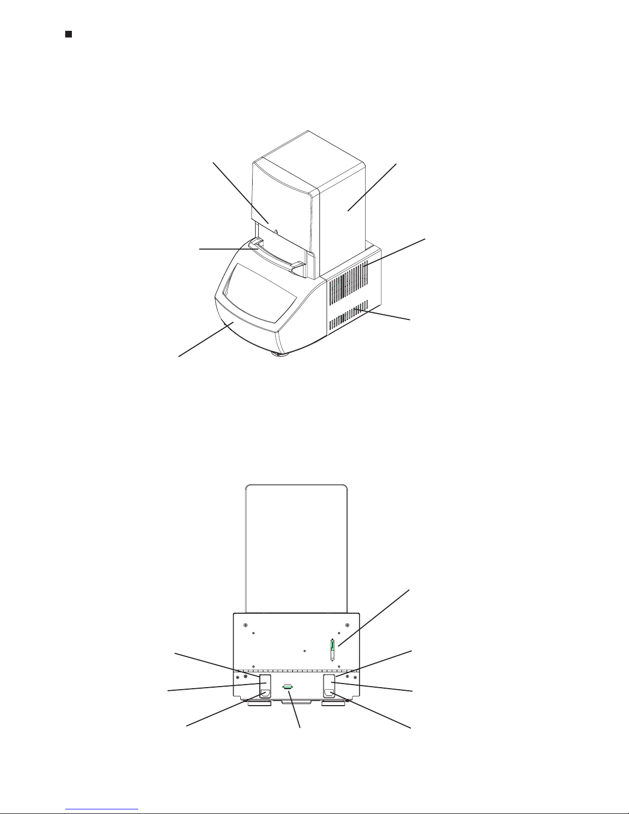
Back View
(Figure 2-2)
Front View
(Figure 2-1)
Power cord jack
(some models)
Power switch
(fuses, some
models)
DAQ (data acquisition)
cable port
Serial cable port
Power module,
left configuration
(standard)
Power cord jack
Power switch
(fuses)
Power module,
right configuration
(some models)
Optical tower
Cycler drawer
Air exhaust vents
(also on other side)
Air intake vents
(also on other side)
Blue protocolindicator light
Blue trigger handle
(door mechanism)
Page 15

Tech Support: (888) 652-9253 • Sales: (888) 735-8437 • tech@mjr.com • www.mjr.com 2-3
Layout and Specifications
Specifications
Thermal range: 0˚ to 105˚C, but not more than 30˚C
below ambient temperature
Accuracy: ±0.3˚C of programmed target @ 90˚C,
NIST-traceable
Thermal homogeneity: ±0.4˚C well-to-well within 30 seconds of
arrival at 90˚C
Ramping speed: Up to 3.0˚C/sec
Sample capacity: 96-well microplate (low-profile) or
96 x 0.2ml strip tubes (low-profile)
Line voltage: 100-240VAC
Frequency: 50-60Hz
Power: 850W maximum
Fuses: Two 6.3A, 250V Type S505, fast acting
(user changeable)
Two 8.0A, 250V Type S505, fast acting
(inaccessible)
Weight: 27kg (excluding computer and
monitor)
Size: 47cm deep x 34cm wide x 60cm high
(excluding computer and monitor)
Fluorescence Excitation Range: 450-495nm
Fluorescence Detection Range: 515-545nm
Page 16

2-4 Tech Support: (888) 652-9253 • Sales: (888) 735-8437 • tech@mjr.com • www.mjr.com
Opticon System Operations Manual
Gradient Specifications
Accuracy: +0.3°C of target at end columns within
30 seconds (NIST-traceable)
Column uniformity:
+0.4°C, in column, well–to–well, within
30 seconds of target attainment
Calculator accuracy:
+0.4°C of actual column temperature
(NIST-traceable)
Lowest programmable 30°C
temperature:
Highest programmable 105°C
temperature:
Gradient range: from 1°C up to 24°C
(temperature differential)
Computer Specifications
(minimum specifications for the computer provided with the Opticon system)
Processor: 2.4GHz processor
Operating System: Windows XP Pro
Display: 15 inch flat-screen monitor
Memory: 256 MB RAM
Storage: 40GB hard drive
Data Acquisition Board: National Instruments PCI-6036E
200kS/s (samples per second)
Page 17

3-1
3. Installation and Operation
Unpacking the Opticon Unit, 3-2
Packing Checklist, 3-2
Setting Up the DNA Engine Opticon System, 3-3
Environmental Requirements, 3-3
Power Supply Requirements, 3-4
Air Supply Requirements, 3-4
Ensuring an Adequate Air Supply, 3-4
Ensuring That Air Is Cool Enough, 3-4
Troubleshooting Air Supply Problems, 3-5
Turning the Opticon Unit and Computer On and Off, 3-5
Opening and Closing the Cycler Drawer, 3-6
Loading Sample Vessels into the Block, 3-6
Page 18

3-2 Tech Support: (888) 652-9253 • Sales: (888) 735-8437 • tech@mjr.com • www.mjr.com
Opticon System Operations Manual
Unpacking the Opticon™ Unit
Please follow these instructions for unpacking the Opticon unit to reduce the risk of personal injury or damage to the instrument.
Important: DO NOT lift the instrument out through the top of the box.
Important: DO NOT use the blue handle to lift the instrument at any time.
• Cut the band securing the cardboard cover to the support base.
• Open the top of the cardboard cover.
• Remove the top foam insert.
• Remove the accessory box (contents listed below).
• Lift the cardboard cover up and off of the instrument.
• Firmly grasp the sides of the instrument from beneath to support the weight of the
cycler and the optical tower. Carefully lift the instrument off of the shipping support. Do not lift the instrument by the blue handle or the cycler drawer.
Packing Checklist
After unpacking the DNA Engine Opticon® continuous fluorescence detection system, check
to see that you have received the following:
1. One DNA Engine Opticon unit (Opticon detector with DNA Engine
®
thermal cycler)
2. One computer with keyboard, mouse, monitor, cables, & installed software (Opticon
Monitor and Windows XP pro)
• One serial cable for connecting the Opticon unit’s serial port (figure 2-2) to the
computer serial port
• One data acquisition cable for connecting the Opticon unit’s DAQ port (figure 2-
2) to the data acquisition card in the computer
3. One Opticon accessory pack including:
• One power cord for the Opticon unit
• Two spare fuses
•
DNA Engine Opticon® Continuous Fluorescence Detection System Operations
Manual
(this document)
• Opticon Monitor
™
software CD ROM
• Consumables samples including 0.2ml low-profile strip tubes in opaque white
(MJ Research catalog no. TLS-0851), optical flat caps for 0.2ml tubes and plates
(MJ Research catalog no. TCS-0803), and low-profile Multiplate
™
96-well micro-
plates in opaque white (MJ Research catalog no. MLL-9651)
Page 19

Tech Support: (888) 652-9253 • Sales: (888) 735-8437 • tech@mjr.com • www.mjr.com 3-3
Installation and Operation
If any of these components are missing or damaged, contact MJ Research, Incorporated or
the authorized distributor from whom you purchased the DNA Engine Opticon system to
obtain a replacement. Please save the original packing materials in case you need to return
the DNA Engine Opticon system for service. See Appendix C for shipping instructions.
Setting Up the DNA Engine Opticon System
The Opticon system requires a location with three power outlets to accommodate the
Opticon unit, the computer, and the monitor. A location with network access (Ethernet
10/100BaseT) is recommended if you wish to transfer setup and analysis files between
the computer running the Opticon unit and other computers.
The DNA Engine Opticon system requires only minimal assembly. Insert the power cord
plug into its jack at the back of the instrument, just below the power switch (see figure 22 for the location of the jack). Then, plug the power cord into a standard 110V or 220V
electrical outlet. The Opticon unit will accept 220V automatically, as does the monitor.
However, you must set the voltage on the computer. See the “Power Supply Requirements”
section below for more information.
Before launching the Opticon Monitor software (see Chapter 5), be sure that the Opticon
unit is connected to the computer. There are two cables that connect the Opticon unit to
the computer. Connect the serial cable to the serial cable port on the Opticon unit (see
figure 2-2) and serial port #2 on the computer. Connect the data acquisition cable to the
DAQ port on the Opticon unit (see figure 2-2) and the data port on the computer.
Note: The DAQ cable has high-density connectors; take care not to bend any of the pins.
Environmental Requirements
For reasons of safety and performance, ensure that the area where the DNA Engine
Opticon system is installed meets the following conditions:
• Nonexplosive environment
• Normal air pressure (altitude below 2000m)
• Ambient temperature 15˚–31˚C
• Relative humidity above 10% and up to 80%
• Unobstructed access to air that is 31˚C or cooler (see below)
• Protection from excessive heat and accidental spills. (Do not place the DNA Engine
Opticon system near such heat sources as radiators, and protect it from danger of
having water or other fluids splashed on it, which can cause electrical short circuits.)
Page 20

3-4 Tech Support: (888) 652-9253 • Sales: (888) 735-8437 • tech@mjr.com • www.mjr.com
Opticon System Operations Manual
Power Supply Requirements
The DNA Engine Opticon unit requires 100-240VAC, 50-60Hz and a grounded outlet.
The DNA Engine Opticon unit can use current in the specified range without adjustment,
so there is no voltage-setting switch. The monitor can also accept either 110 or 220V
power without adjustment.
Important! For 220V operation of the computer, the red voltage-setting
switch located on the back of the computer, near the power cord
jack, must display 230V rather than 115V.
The Opticon unit is equipped with a power-entry module that accepts cordsets with an
IEC 60320-1 type C13 connector (this is the same standard configuration used by many
computer manufacturers for their equipment). All cordsets used with the Opticon unit must
be rated to carry at least 10A at 125V or 250V, the latter specification depending upon
the supply voltage used. Additionally, the cordset must meet all other applicable national
standards—thus at a minimum, the cordset should carry the mark of a nationally recognized testing agency appropriate to your nation.
Note: Do not cut the supplied 120V power cord and attach a different connector. Use a one-
piece molded connector of the type specified above.
Air Supply Requirements
The DNA Engine Opticon unit requires a constant supply of air that is 31˚C or cooler in
order to remove heat from the heat sink. Air is taken in from the lower vents located on
the sides of the instrument and exhausted from the upper vents on both sides (see figure
2-1). If the air supply is inadequate or too hot, the instrument can overheat, causing performance problems and even automatic shutdowns.
Ensuring an Adequate Air Supply
• Do not block air intake vents (see figure 2-1).
Position the DNA Engine Opticon unit at least 10cm from vertical surfaces and other thermal
cyclers or heat-generating equipment (greater distances may be required; see below).
• Do not allow dust or debris to collect in the air intake vents.
Ensuring That Air Is Cool Enough
• Do not position two or more DNA Engine Opticon units (or other instruments) so that hot
exhaust air blows directly into the air intake vents.
• Confirm that the DNA Engine Opticon unit receives air that is 31˚C or cooler by measuring the temperature of air entering the machine through its air intake vents.
Page 21

Tech Support: (888) 652-9253 • Sales: (888) 735-8437 • tech@mjr.com • www.mjr.com 3-5
Installation and Operation
Place the DNA Engine Opticon unit where you plan to use it, and turn it on. Try to
reproduce what will be typical operating conditions for the machine in that location,
particularly any heat-producing factors (e.g., nearby equipment running, window blinds
open, lights on). Run a typical protocol for 30 minutes to warm up the DNA Engine
Opticon unit, then measure the air temperature at the air intake vents. If more than one
machine is involved, measure the air temperature for each.
If the air intake temperature of any machine is warmer than 31˚C, consult Table 3-1 for
possible remedies. After implementing possible remedies, verify that the temperature of
the air entering the air intake vents has been lowered, using the procedure outlined above.
Table 3-1 Troubleshooting Air Supply Problems
Cause Possible Remedies
Air circulation is poor. Provide more space around instrument or adjust room
ventilation.
Ambient air temperature Adjust air conditioning to lower ambient air
is high. temperature.
Instrument is in warm part Move instrument away from, or protect instrument from,
of room. such heat sources as radiators, heaters, other equip-
ment, or bright sunlight.
Instruments are crowded. Arrange machines so that warm exhaust air does not
enter intake vents.
Turning the Opticon Unit and Computer On and Off
Locate the power switch on the back, left-side of the Opticon unit (back, right-side on
some models) just above the power cord (see figure 2-2). To turn the Opticon unit on,
press the switch so that the side marked “1” is depressed. The thermal cycler requires
several minutes to warm up after the Opticon unit is powered up. To turn the Opticon unit
off, depress the “0” side of the power switch.
Be sure that the Opticon unit is connected to the computer and turned on prior to launching the Opticon Monitor software. The blue protocol-indicator light on the front of the
Opticon unit (see figure 2-1) is illuminated only during a protocol run.
Press the power button on the front of the computer once to turn the computer on. Select
Shutdown
from the
Start
menu to turn the computer off. Press the power button on the
front of the monitor once to turn it on, and press it again to turn the monitor off.
Page 22
3-6 Tech Support: (888) 652-9253 • Sales: (888) 735-8437 • tech@mjr.com • www.mjr.com
Opticon System Operations Manual
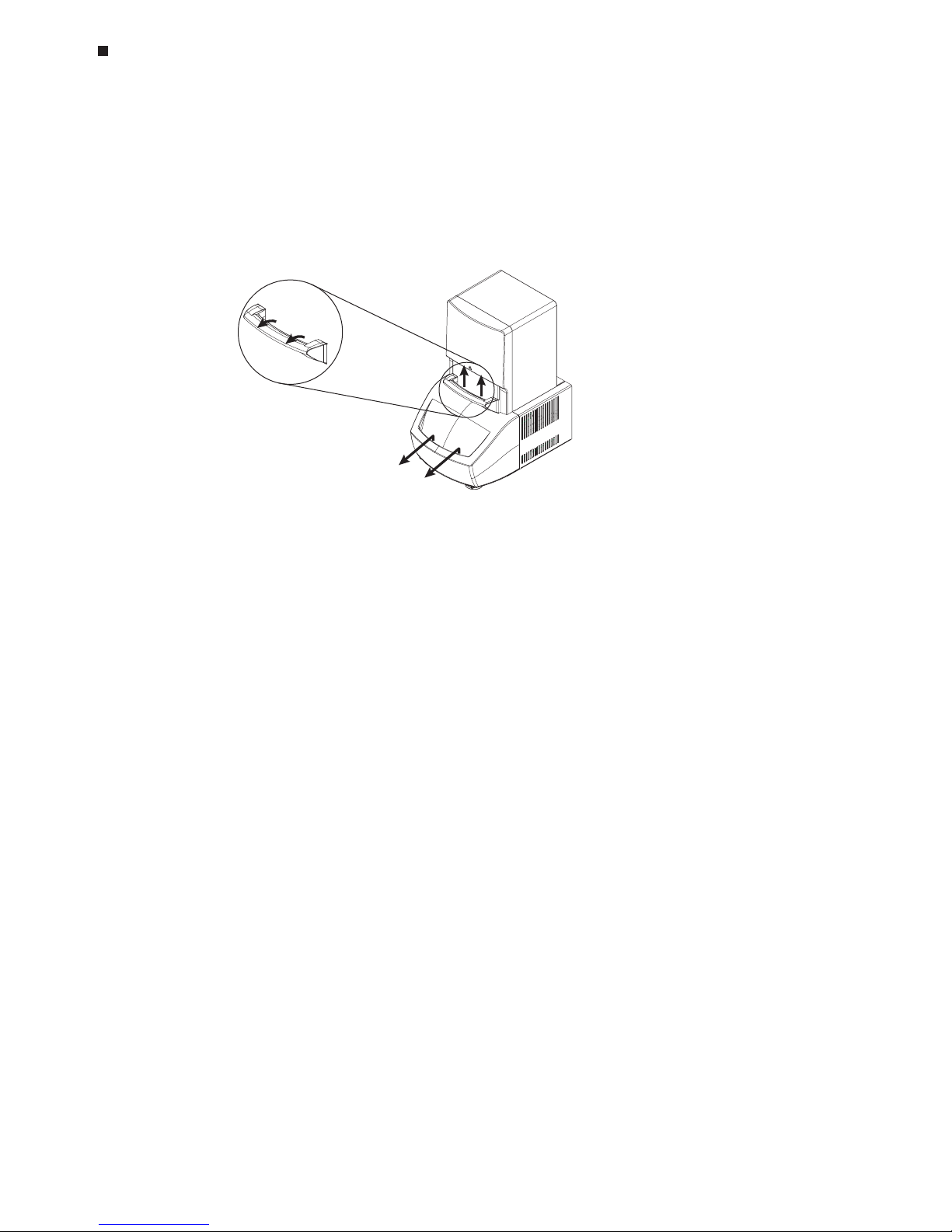
Opening and Closing the Cycler Drawer
To gain access to the Opticon unit’s thermal cycling block, first squeeze the blue trigger
handle (1) and allow the spring-loaded door to lift up (2). Then, use the hand hold on the
drawer front to slide the cycler drawer out toward you exposing the 96-well thermal cycler block (3).
To return the Opticon unit to the closed position, slide the cycler drawer back into the
instrument and lower the blue handle to secure the cycler drawer. It is not necessary to
squeeze the trigger handle.
Note: Do not open the cycler drawer while the blue protocol-indicator light is illuminated.
Opening the door, particularly during a scan of the plate, may interrupt the software’s
control of the protocol.
Loading Sample Vessels into the Block
Important! Do not use full height 0.2ml tubes or full height unskirted
microplates. Refer to the “Selecting the Correct Sample Vessel” section
in Chapter 4 for tube and microplate recommendations.
To ensure uniform heating and cooling of samples, sample vessels must be in complete
contact with the block. Adequate contact is ensured by doing the following:
• Ensure that the block is clean before loading samples (see Chapter 9 for cleaning
instructions).
• Firmly press strips of 0.2ml low-profile tubes, or a 96-well, low-profile microplate into
the block wells (see the “Selecting the Correct Sample Vessel” section in Chapter 4).
• MJR strongly recommends that oil not be used to thermally couple sample vessels to
the block.
Tip: Spin down reactions in tubes or microplates prior to loading into the thermal-cycler
block. Air bubbles in samples or liquid on the plate deck can adversely affect results.
1.
2.
3.
Page 23

4-1
4. Compatible Chemistries,
Sample Vessels, and Sealing
Options
Optical System, 4-2
Compatible Chemistries, 4-2
SYBR Green I, 4-2
Molecular Beacons, 4-3
Hydrolysis Probes (TaqMan Probes), 4-3
Scorpions Probes, 4-4
Amplifluor Universal Detection System, 4-4
Selecting the Correct Sample Vessel, 4-5
Vessels Optimized for Fluorescence Detection and Thermal Cycling, 4-5
Sealing Sample Vessels, 4-5
Sealing with Optical Caps and the Heated Lid, 4-6
Sealing with Chill-out™ 14 Liquid Wax, 4-6
Sample Vessel and Sealing Selection Chart for Optical Assays, 4-7
Reaction Volume Recommendations, 4-8
Page 24

4-2 Tech Support: (888) 652-9253 • Sales: (888) 735-8437 • tech@mjr.com • www.mjr.com
Opticon System Operations Manual
Optical System
The Opticon™ detector uses an array of 96 blue LEDs to sequentially illuminate each of
the 96 wells in the cycler block. The LEDs efficiently excite fluorescent dyes with excitation spectra in the 450 to 495nm range. The Opticon detector is optimized to detect dyes
with emission spectra in the 515 to 545nm range, such as SYBR Green and FAM.
The Opticon detector is calibrated at the factory and requires no calibration before use.
See Chapter 10, “Troubleshooting” for instructions on testing detector calibration and
recalibrating.
Compatible Chemistries
The Opticon detector is compatible with popular dye chemistries including SYBR Green
I, molecular beacons, hydrolysis probes (TaqMan probes), Scorpions probes, and the
Amplifluor system. In addition to performing real-time quantification and DNA melting
profiles, the Opticon system is also useful as a temperature-controlled fluorimeter for a
number of applications including ligand binding and protein structure studies. If you have
questions regarding the compatibility of a particular chemistry with the Opticon detector,
contact MJ Research technical support at 888-652-9253.
SYBR Green I
SYBR Green I (available from Molecular Probes, Inc. of Eugene, Oregon) is a dsDNA
binding dye thought to bind in the minor groove. The fluorescence of SYBR Green I is
greatly enhanced upon binding dsDNA. This characteristic makes it ideal for detection
of amplification products. The maximum absorbance of SYBR Green I is ~497nm and
the emission maximum is ~520nm*.
SYBR Green I has several advantages for detection of nucleic acids in real time. Because
SYBR Green I binds to all dsDNA, it does not have to be customized for individual templates thereby providing the advantages of quick protocol adaptation and relatively low
cost. Further, SYBR Green I is very sensitive because multiple dye molecules bind to a
single amplification product. However, because SYBR Green I binds to all dsDNA, false
positive signals from primer-dimers, secondary structure, or spurious priming can interfere with accurate quantification. Measuring fluorescence at elevated temperatures may
help reduce the detection of nonspecific products
1
. Performing a melting curve to analyze product homogeneity can also aid in analyzing quantification results obtained with
SYBR Green I.
MJR recommends using buffers containing 5% dimethyl sulfoxide (DMSO) with a concentration of 1X or less SYBR Green I with the Opticon detector. For additional information
on optimizing protocols using SYBR Green I with thermostable enzymes available from
MJ Research, contact MJ Research technical support at 888-652-9253.
1
Morrison, T.B., J.J. Weis and C.T. Wittwer. 1998. Biotechniques 24:954-962.
*Molecular Probes, Inc.
Page 25

Tech Support: (888) 652-9253 • Sales: (888) 735-8437 • tech@mjr.com • www.mjr.com 4-3
Compatible Chemistries, Sample Vessels, and Sealing Options
Molecular Beacons
Molecular beacons are dual-labeled oligonucleotide probes designed to form stem-loop
structures in the absence of target. In the hairpin configuration, the fluorophore at one
end of the molecule is brought into close proximity with a quenching moiety at the other
end of the molecule. When the fluorophore is excited in this configuration, it transfers
energy to the quencher rather than emitting that energy as light, in a process known as
fluorescence resonance energy transfer (FRET). A “dark” quencher is often used, so the
energy transferred from the fluorophore is emitted in the infrared as opposed to the visible range. If a second fluorophore is used as a quencher, the transferred energy is emitted as light at the quenching fluorophore’s characteristic wavelength.
Molecular beacons are designed such that the loop, which is usually 15-30 nucleotides in
length, is complimentary to the target sequence. The arms flanking the loop, which are
usually 5–7 nucleotides in length, are designed such that they are complementary and
favor formation of a stem structure. A fluorophore is attached to the end of one arm, and a
quencher is attached to the other. Molecular beacons must be carefully designed such that
at the annealing temperature of the reaction hairpins form in the absence of template, but
that in the presence of template, the annealing of the loop sequence to the target is energetically favorable. When the loop of a molecular beacon hybridizes to the target sequence,
the conformational change of the probe separates the fluorophore and the quencher.
When the fluorophore is excited, it now emits light at its characteristic wavelength.
One advantage of molecular beacons is that unlike SYBR Green, molecular beacons specifically detect the target of interest. Great sensitivity, including detection of single
nucleotide polymorphisms (SNPs), is possible with carefully designed molecular beacons
and optimized reaction conditions (temperature, buffer). However, each probe must be
carefully and uniquely designed for the detection of a specific target.
Molecular beacons are a technology patented by the Public Health Research Institute of
New York, NY and are available from a number of licensed suppliers. When designing
molecular beacons for use with the Opticon detector, fluorophores with excitation and
emission spectra falling within the Opticon detector’s excitation (450-490nm) and detection (515-545nm) ranges, such as FAM, can be used. Either dark quenchers or a quenching fluorophore may be used with the Opticon detector. However, because the Opticon
detector is a single-color detection system, light from a quenching fluorophore can not be
separately monitored. Dark quenchers tend to give cleaner signal because there is no
overlapping signal from light emitted by the quenching fluorophore.
Hydrolysis Probes (TaqMan Probes)
TaqMan probes are a patented technology available from a number of licensed suppliers. They are oligonucleotide probes whose fluorescence is dependent on the amplification of a target sequence. TaqMan probes are designed to anneal to the target sequence
between the forward and reverse primers. A reporter fluorophore is attached to the 5’
end of the probe and a quencher to the 3’ end.
Page 26

4-4 Tech Support: (888) 652-9253 • Sales: (888) 735-8437 • tech@mjr.com • www.mjr.com
Opticon System Operations Manual
When the intact probe anneals to the target sequence, excitation of the reporter is quenched
because of its proximity to the 3’ quencher. However, as extension proceeds, the 5’ exonuclease activity of the polymerase cleaves the probe, separating the reporter from the
quencher. TaqMan probes work well with enzymes derived from Thermus species, such
as DyNAzyme™ II DNA polymerase from Thermus brockianus, available from MJ Research,
Inc. Liberated reporter molecules accumulate as the number of cycles increases, such that
the increase in fluorescence is proportional to the amount of amplified product.
One advantage of TaqMan probes, particularly for quantification, is that fluorescence is
dependent not only on the presence of a specific target, but also on amplification of that
target. However, like molecular beacons, TaqMan probes must be individually designed
for specific targets. See the “Molecular Beacons” section above for recommendations on
the use of specific fluorophores and quenchers with the Opticon detection system.
Scorpions Probes
Scorpions probes (available from licensed suppliers) contain both an amplification primer
and a target-specific probe separated by an amplification blocker. The probe portion is
flanked by complementary sequences favoring formation of a stem structure which brings
a fluorophore and a quencher into close proximity.
During amplification, extension of the target sequence proceeds from the primer portion
of the Scorpions probe. As the reaction cools following denaturation, a uni-molecular
rearrangement occurs such that the Scorpions probe sequence binds to the amplified target sequence, separating the complementary stem sequences and thus the fluorophore
and quencher. Since the Scorpions probe is integrated into the product, there is a direct
relationship between the number of targets generated and the amount of fluorescence.
See the “Molecular Beacons” section above for recommendations on the use of specific
fluorophores and quenchers with the Opticon detection system.
Amplifluor Universal Detection System
The Amplifluor system (available from Intergen Company of Purchase, NY) makes use of
a universal primer that emits a fluorescence signal only following incorporation of the
primer into an amplification product. The universal primer consists of a 18 base primer
tail ("Z sequence") coupled to a hairpin sequence labeled with a fluorophore and a
quencher. First, the target is amplified using target-specific primers, one of which has the
Z sequence added to its 5' end. In the following round of amplification, the complement
to the Z sequence is incorporated into the product. The universal primer then anneals to
the complement of the Z sequence and extension proceeds. In the next cycle, extension
proceeds through the universal primer incorporating it into the amplification product. In
the process, the hairpin is unfolded separating the fluorophore and quencher and emitting a fluorescence signal that is proportional to the amount of amplified product.
See the “Molecular Beacons” section above for recommendations on the use of specific
fluorophores and quenchers with the Opticon detection system.
Page 27

Tech Support: (888) 652-9253 • Sales: (888) 735-8437 • tech@mjr.com • www.mjr.com 4-5
Compatible Chemistries, Sample Vessels, and Sealing Options
Selecting the Correct Sample Vessel
Important! Do not use full height 0.2ml tubes or full height unskirted
microplates. Full height 0.2ml tubes and most unskirted microplates do
not provide sufficient clearance between the sample block and lid-heater
assembly. Do not force the cycler drawer closed.
For proper clearance in the Opticon unit, the distance from the bottom of a tube/plate to
the cap rim can not exceed 17.5mm. In general, fully-skirted 96-well microplates, such
as MJ Research Microseal
®
and Hard-Shell® microplates, provide sufficient clearance when
sealed with either domed or flat optical caps (see the "Sample Vessel and Sealing Selection Chart for Optical Assays" below). If unskirted microplates are used, low-profile plates,
such as the MJ Research MLL-series Multiplate
™
microplates, are required.
Low-profile 0.2ml strip tubes, such as MJ Research TLS-series tubes, are recommended
for small numbers of samples. Full-height 0.2ml tubes do not provide sufficient clearance.
Vessels Optimized for Fluorescence Detection and Thermal
Cycling
For optimal sensitivity in fluorescence-detection assays, we recommend thin-walled 0.2ml
tube strips and microplates with opaque-white wells. MJ Research, Inc. offers microplates
and tubes with opaque white or clear wells designed for fluorescence detection assays
and optimized to ensure a precise fit in the cycler block (see the "Sample Vessel and
Sealing Selection Chart for Optical Assays" below).
Microplates and tubes with black wells may be useful in applications requiring very low
levels of background. However, signal strength is significantly reduced when plates and
tubes with black wells are used.
Note: In-factory calibration of the Opticon detector is performed with opaque-white plates.
If you are using natural (clear) or black plates, refer to Chapter 10 for instructions on
performing a calibration test and recalibrating.
Sealing Sample Vessels
Steps must be taken to prevent the evaporation of water from reaction mixtures during thermal cycling so as to avoid changing the concentration of reactants. Only a layer of oil or
wax, such as Chill-out liquid wax, will completely prevent evaporation from sample vessels. However, an adequate degree of protection can be achieved by sealing with optical
caps, then cycling the samples using the heated lid to prevent condensation/refluxing.
Page 28

4-6 Tech Support: (888) 652-9253 • Sales: (888) 735-8437 • tech@mjr.com • www.mjr.com
Opticon System Operations Manual
Sealing with Optical Caps and the Heated Lid
The heated inner lid maintains the upper part of sample vessels at a higher temperature
than the reaction mixture. This prevents condensation of evaporated water vapor onto
the vessel walls, so that solution concentrations are unchanged by thermal cycling. The
heated lid also exerts pressure on the tops of vessels loaded into the block, helping to
maintain a vapor-tight seal and to firmly seat tubes or microplates in the block for the
most efficient transfer of heat to and from the samples.
Optical caps must be used along with the heated lid to prevent evaporative losses. Ultraclear, optical cap strips (available from MJ Research, Inc.) provide high light transmission for fluorescence detection and vapor-tight sealing. Tight-fitting caps do the best job
of preventing vapor loss.
Note: When tubes are cooled to below-ambient temperatures, a ring of condensation may
form in tubes above the liquid level but below the top of the sample block. This is not a
cause for concern since it occurs only at the final cool-down step when thermal cycling is
finished.
Sealing with Chill-out™ Liquid Wax
Clear Chill-out liquid wax (available from MJ Research, Inc.) may be used to seal sample
vessels for optical assays. Clear Chill-out liquid wax is the same easy-to-use alternative to
oil as the standard, red-colored Chill-out wax. However, clear Chill-out wax provides excellent light transmission for optimal performance in optical assays. Chill-out liquid wax
provides 100% prevention of condensation and vapor loss. At room temperature and
above, this overlay is transparent and can be applied by pipet. Chill-out liquid wax solidifies below 14°C. Use only a small amount of Chill-out liquid wax; 1-3 drops (15-50µl)
are usually sufficient. (Include this volume in the total volume when setting up a calculated-control protocol.) Be sure to use the same amount of wax in all samples vessels to
ensure a uniform thermal profile.
Page 29

Tech Support: (888) 652-9253 • Sales: (888) 735-8437 • tech@mjr.com • www.mjr.com 4-7
Compatible Chemistries, Sample Vessels, and Sealing Options
Sample Vessel and Sealing Selection Chart for Optical Assays
The following sample vessels and sealing options are recommended for use with the DNA
Engine Opticon® system and are available from MJ Research, Inc. To place an order, call
888-729-2165 or fax 888-729-2166.
tcudorP
golataChcraeseRJM
rebmuN
sthgilhgihtcudorP
slesseV
eliforP-woL
sebutlm2.0
8fospirts
)etihweuqapo(1580-SLT
)raelc(1080-SLT
fosrebmunllamsroflaedI•
selpmas
mumixamofsllewetihwesU•
langis
mrofinurofsllewraelcesU•
gniweivelpmasdnalangis
™etalpitluMeliforP-woL
detriksnu
llew-69
setalporcim
)etihweuqapo(1569-LLM
)raelc(1069-LLM
selpmas69nahtrewefroflaedI•
ezisottucebnacsetalporcim---
mumixamofsllewetihwesU•
langis
mrofinurofsllewraelcesU•
gniweivelpmasdnalangis
llew-69®laesorciM
s
etalporcimdetriks
)etihweuqapo(1569-PSM
)raelc(1069-PSM
mumixamofsllewetihwesU•
langis
mrofinurofsllewraelcesU•
gniweivelpmasdnalangis
llew-69®llehS-draH
setalporcimdetriks
sllewetihw/llehsetihw5569-PSH
sllewetih
w/llehskcalb5669-PSH
sllewetihw/llehsder5169-PSH
sllewetihw/llehswolley5269-PSH
sllewetihw/llehseulb5369
-PSH
sllewetihw/llehsneerg5469-PSH
sllewraelc/llehsetihw1069-PSH
sllewraelc/llehskcalb1669-PSH
sllewraelc
/llehsder1169-PSH
sllewraelc/llehswolley1269-PSH
sllewraelc/llehseulb1369-PSH
sllewraelc/llehsneerg1469-
PSH
selpmas69roflaedI•
talfyletulosbasniameretalP•
rof,gnilcyclamrehtgnirud
noitcellocthgilmrofinu
rofdoog
erasllehsderoloC•
gnidoc-roloc
snoitpOgnilaeS
.spactalflacitpO
8fospirts
3080-SCT
thgilhgihrofraelc-artlU•
noissimsnart
lµ5>semulovgnilcyclamrehT•
diuqiL
™tuO-llihC
edarg-lacitpo,xaW
1141-OHC
yalrevoliolarenimsecalpeR•
noissimsnartthgilhgiH•
lµ2>semulovgnilcyc
-lamrehT•
Page 30

4-8 Tech Support: (888) 652-9253 • Sales: (888) 735-8437 • tech@mjr.com • www.mjr.com
Opticon System Operations Manual
Reaction Volume Recommendations
Reaction volumes of 20-100µl are recommended for most applications. However, it is
beneficial to empirically optimize reagent concentrations and sample volumes with the
Opticon detector as the sensitivity of the optical system often allows a cost-saving reduction in reagent concentrations. Volumes as low as 10µl can be used, though sensitivity is
slightly reduced.
The maximum recommended sample volume is 100µl. Volumes exceeding 100µl do not
maintain adequate contact with the wells of the sample block resulting in nonuniform
heating and cooling within the sample.
The reaction volume is used to calculate the temperature of the samples during a calculated-control run (see the “Temperature Control Method” section in Chapter 6). Therefore,
thermal accuracy is optimized when all samples contain identical volumes.
Page 31

5-1
5. Introduction to Opticon
Monitor™ Software
How Opticon Monitor Software Works, 5-2
Launching and Navigating Opticon Monitor Software, 5-3
Exiting Opticon Monitor Software, 5-5
Opticon Monitor File Extensions, 5-6
Which Version of Opticon Monitor Software Are You Running?, 5-6
Viewing Usage and Message Logs, 5-6
Page 32

5-2 Tech Support: (888) 652-9253 • Sales: (888) 735-8437 • tech@mjr.com • www.mjr.com
Opticon System Operations Manual
Opticon Monitor software controls all operations on the DNA Engine Opticon® continuous fluorescence detection system. This chapter will introduce you to the Opticon Monitor software and discuss the basics of launching and navigating the software. Chapter 6
describes experimental setup and programming. Chapter 7 discusses run initiation and
status, and Chapter 8 focuses on data analysis. This manual documents version
1.08 of the Opticon Monitor software.
How Opticon Monitor Software Works
The intuitive Opticon Monitor software is structured such that there are just three phases
from protocol creation to analyzed results.
1. Experimental setup and programming. All setup and programming operations are accessed from the master file window. The master file orchestrates the run by
specifying which combination of plate and protocol files to apply to a particular run.
Users can create new files or apply existing files, in their current form or after editing.
2. Run initiation and status. After creating a plate and a protocol setup, or select-
ing a plate and a protocol file, a run can be initiated. The user has the option to stop the
run at any time and to skip protocol steps. The status screen can be used to monitor the
progress and thermal profile of the run. Data collection can be monitored during the run
by plotting fluorescence intensity vs. cycle number.
3. Data analysis. Starting copy number can be quantified by using the software to set
the c(t) (cycle threshold) line, view and adjust an automatically-generated standard curve,
and apply unknowns to the curve. Products can be identified by melting profile using the
software to plot fluorescence vs temperature, and/or the negative first derivative (-dI/dt)
of that graph.
Page 33

Tech Support: (888) 652-9253 • Sales: (888) 735-8437 • tech@mjr.com • www.mjr.com 5-3
Introduction to Opticon Monitor Software
Launching and Navigating Opticon Monitor Software
Opticon Monitor software is pre-installed on the computer provided with the Opticon
™
unit. The Opticon Monitor software is compatible with Windows 2000 and Windows XP
operating systems. Opticon Monitor software can control the Opticon unit only when running on the computer supplied with the system, which has special hardware required for
data acquisition. Nonetheless, Opticon Monitor software can be installed on any computer running Windows 2000 or Windows XP for the purposes of setting up protocols or
analyzing data.
To launch the Opticon Monitor software, choose
Programs
from the Windows
Start
menu,
and then
Opticon Monitor
. Upon launching the Opticon Monitor software, the Opticon
Monitor window will appear displaying a new master file template. Alternatively, double
click on an existing Opticon Monitor master, plate, protocol, or data file to launch Opticon Monitor and display the chosen file.
4. Log box
1. Toolbar 2. Pull-down menus
3. Setup/analysis display window
(master file)
Page 34
5-4 Tech Support: (888) 652-9253 • Sales: (888) 735-8437 • tech@mjr.com • www.mjr.com
Opticon System Operations Manual
Opticon Monitor window features include:
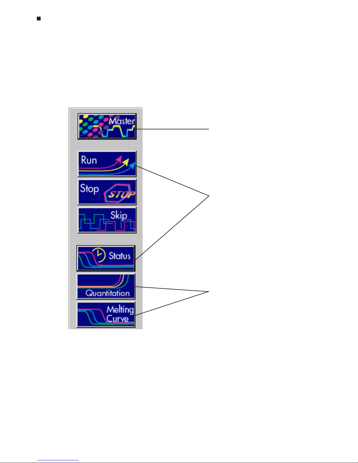
1. Toolbar: The toolbar contains both menu buttons and run status information. The
menu buttons located on the toolbar are the primary means of navigation between
the setup/programming, run/status and analysis windows:
Experimental setup & programming
Run initiation and monitoring
Data analysis
Page 35

Tech Support: (888) 652-9253 • Sales: (888) 735-8437 • tech@mjr.com • www.mjr.com 5-5
Introduction to Opticon Monitor Software
The run status box on the toolbar indicates if a protocol or infinite incubation step is
running. It lists the time remaining in the run, the current step and cycle counts, and
the current temperatures.
2. Pull-down menus: The pull-down menus provide access to numerous functions
including the ability to print and export data as well as set the default options for
data analysis.
3. Setup/analysis display window: The window displays the selected setup, sta-
tus, or analysis screen.
4. Log box: The log box lists the instrument operation log including any errors encoun-
tered.
Exiting Opticon Monitor Software
Exit Opticon Monitor software by selecting
Exit
from the
File
menu, or by clicking the
close button in the upper-right corner of the title bar. If a protocol is running, it must be
stopped prior to exiting Opticon Monitor software.
Page 36

5-6 Tech Support: (888) 652-9253 • Sales: (888) 735-8437 • tech@mjr.com • www.mjr.com
Opticon System Operations Manual
Opticon Monitor File Extensions
When saving files, the Opticon Monitor software automatically adds one of the following file
extensions:
.mast Master file: Controls a run by specifying which plate and protocol
files to apply during the run.
.plate Plate file: Specifies the contents of the 96 wells, any descriptive well labels that
were assigned, and the amounts of any quantitation standards for use in generating a standard curve.
.prot Protocol file: Specifies the order and parameters of protocol steps including
temperature incubations, plate reads, temperature gradients, goto steps, and
melting curves.
.tad Data file: Contains the fluorescence and temperature data collected during the
run, and any selected options and analysis parameters.
Which Version of Opticon Monitor Software Are You
Running?
To determine which version of Opticon Monitor software is currently installed on your
computer, choose
About
from the
Help
menu. The About window will appear displaying
the Opticon Monitor version number. This manual documents Opticon Monitor software,
version 1.08.
Select
Close
to return to the current setup or analysis screen, or click the X in the upper-
right corner.
Viewing Usage and Message Logs
To view a record consisting of the dates and times that runs were initiated and successfully completed, as well as a record of the master, plate, and protocol files applied during those runs, select
Logs
from the
View
pull-down menu and click the
Usage Log
toggle
tab. The dates and times that the software was launched and quit will also be displayed.
To view a record of operations performed by the Opticon Monitor software, including
any error messages, select
Logs
from the
View
pull-down menu and click the
Message
Log
toggle tab.
Page 37

6-1
6. Experimental Setup and
Programming
Creating a Master File, 6-2
Specifying a User, 6-3
Adding New Users, 6-3
User Password Protection, 6-4
Removing Users, 6-4
Assigning New Plate and Protocol Files to a Master File, 6-4
Creating a Plate File, 6-4
Assigning Well Contents, 6-5
Selecting Wells Using the Plate Diagram, 6-5
Selecting Wells Using the Plate Information Table, 6-6
Specifying Quantitation Standards, 6-7
Assigning Well Descriptions, 6-8
Saving a Plate File, 6-8
Creating a Protocol File, 6-9
Choosing a Temperature and a Lid Control Mode, 6-10
Temperature Control Method, 6-10
Lid Control, 6-11
Saving Temperature and Lid Control Settings, 6-12
Designing and Entering a Protocol, 6-12
Entering a New Protocol, 6-13
Temperature Step, 6-13
Gradient Step, 6-15
Gradient Calculator, 6-17
Plate Read Step, 6-17
Adding Multiple Temperature Steps, Gradient Steps, or Plate Reads, 6-17
Goto Step, 6-18
Melting Curve Step, 6-19
Editing a Protocol Step, 6-20
Deleting a Protocol Step, 6-20
Inserting a Protocol Step Between Existing Steps, 6-20
Melting Curve Analysis, 6-21
Saving a Protocol File, 6-23
Saving a Master File, 6-23
Assigning Existing Plate and Protocol Files to a Master File, 6-23
Reusing Master Files, 6-24
Using the Quick Load Feature, 6-25
Page 38

6-2 Tech Support: (888) 652-9253 • Sales: (888) 735-8437 • tech@mjr.com • www.mjr.com
Opticon System Operations Manual
All setup and programming operations can be accessed from the master file window.
Before running a protocol on the DNA Engine Opticon® system, a master file specifying
all of the parameters for the run can be created. The master file orchestrates the run by
specifying which plate and protocol files to apply to a run. The first section of this chapter
will describe how to create and assign new plate and protocol files to a master file. The
second section will describe how to assign existing plate and protocol files, with or without modifications, to a master file. Finally, instructions for reusing and editing existing
master files will be discussed.
Creating a Master File
Upon launching the Opticon Monitor™ software (see Chapter 5), the Opticon Monitor
window will appear displaying a new master file template.
New master file
Page 39
Experimental Setup and Programming
Tech Support: (888) 652-9253 • Sales: (888) 735-8437 • tech@mjr.com • www.mjr.com 6-3
A master file consists of two component files:
1. Plate file: specifies the contents of the 96 wells, any descriptive well labels that were
assigned, and the amounts of any quantitation standards for use in generating a
standard curve.
2. Protocol file: specifies the order and parameters of temperature incubations, plate
reads, temperature gradients, goto steps, and melting curves.
The
New, Edit, Open
, and
Save
buttons located in the Plate Setup and Protocol Setup
sections of the master file can be used to assign new or existing files to the master file as
described below. The Quick Load feature can be used to quickly assign existing plate
and protocol files to the master file (see the "Using the Quick Load Feature" section at the
end of this chapter).
Specifying a User
The user feature allows users to organize master, plate, protocol and data files by placing them in a
Shared
folder to which all users have read/write access, or into personal
folders which can be password protected. Files in a password-protected folder cannot be
edited or deleted through Opticon Monitor, nor can files be placed in the folder without
the password. However, password-protected files can be read by all users. These files
can be edited by any user if a Save as is first performed and the file is assigned to the
shared folder or that user's folder. This provides all users access to all files, but ensures
that the files in an individual user's password-protected folder are only altered by that
user.
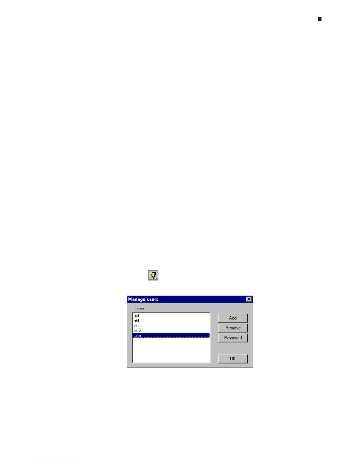
Adding New Users
To add a new user, click the icon in the master file window.
Page 40

6-4 Tech Support: (888) 652-9253 • Sales: (888) 735-8437 • tech@mjr.com • www.mjr.com
Opticon System Operations Manual
In the Manage users window that appears, select
Add
. Enter the new user's name in the
New User window that appears and select
OK
.
User Password Protection
To password protect a user's files, select the name from the Users list in the Manage users
window and then select
Password
. To assign a password, enter the password in the
New
Password
field and again in the
Confirm New Password
field. To change an existing
password, first enter the existing password in the
Old Password
field, and then enter and
confirm the new password. The user will be prompted to enter their password when their
name is selected from the drop-down
User
list in the master file window.
Removing Users
To remove a user from the Opticon Monitor software, select the user's name in the Manage users window and then select
Remove
. You will be asked to confirm deletion of the
user as all data associated with the user will also be deleted.
Assigning New Plate and Protocol Files to a Master
File
Creating a Plate File
A plate file functions to identify the contents of the 96 wells as empty (ignored), blank (for
background subtraction), quantitation standard (for standard-curve generation), or sample
(for unknown and control reactions). A plate file may also contain user-specified well
descriptions, and the amounts and units of any quantitation standards.
Click the
New
button in the Plate Setup section of the master file to create a new plate
file.
In the plate file window, begin by entering the volume of your reactions (in µl) in the
Reac-
tion Volume
field. See the "Reaction Volume Recommendations" section in Chapter 4 for
additional information.
Page 41
Experimental Setup and Programming
Tech Support: (888) 652-9253 • Sales: (888) 735-8437 • tech@mjr.com • www.mjr.com 6-5
Assigning Well Contents
Follow these steps to characterize the contents of wells as empty, blank, quantitation standard, or sample:
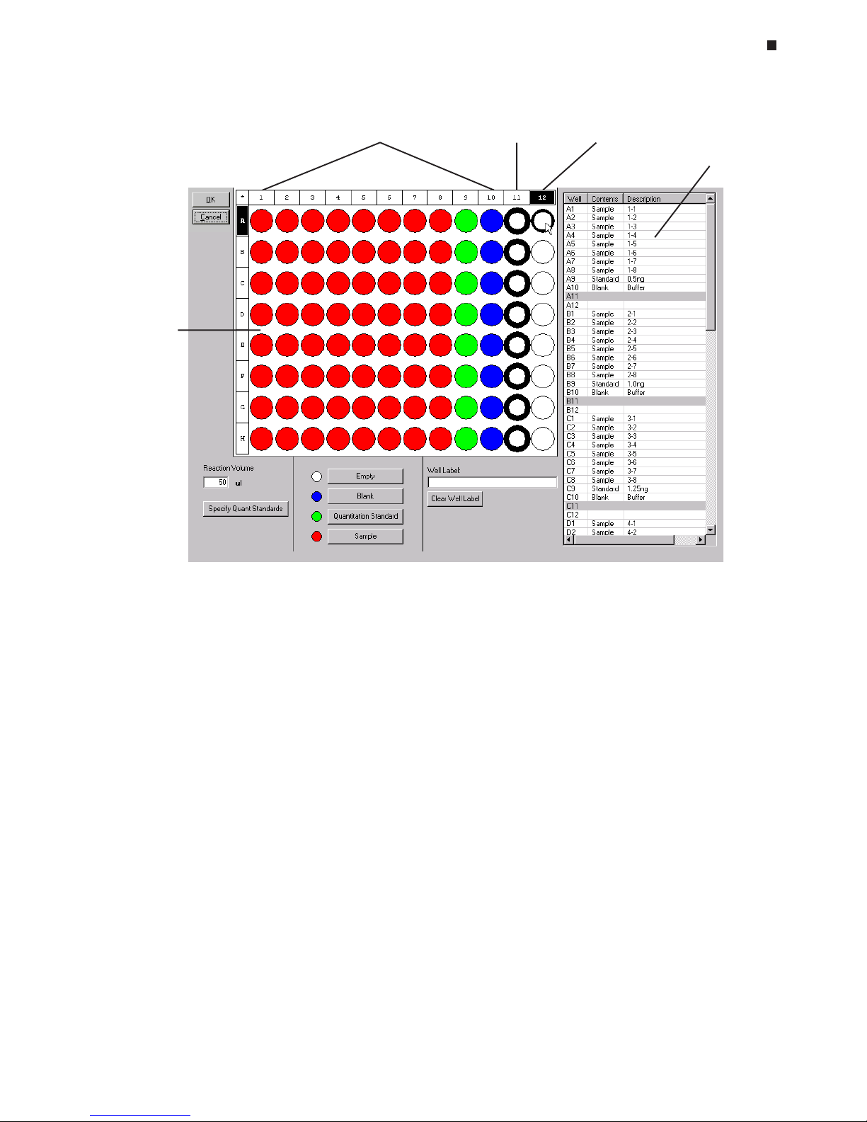
1. Select the well or grouping of wells to which a specific content is to be assigned. You
can select wells by using either the plate diagram or the plate information
table to the right of the diagram.
Selecting Wells Using the Plate Diagram
Move the cursor over an individual well, row letter, or column number to highlight the
well or wells with a thin outline and darken the corresponding well coordinates (see
well A12 in the diagram above). Clicking on highlighted wells will select them. Selected wells appear heavily outlined, and the fields of the corresponding wells are
highlighted in the plate information table (see wells in column 11 in the diagram above).
• Select all wells in the plate by clicking on the * in the upper-left corner of the plate
diagram.
• Select all wells in a column by clicking on the numbered box at the top of the
column. To select multiple columns, hold down the control key and click on the
numbered box at the top of each column to be selected.
Plate
diagram
Wells with assigned
contents
Selected
wells
Highlighted
well
Plate
information
table
Plate file window
Page 42
6-6 Tech Support: (888) 652-9253 • Sales: (888) 735-8437 • tech@mjr.com • www.mjr.com
Opticon System Operations Manual
• Select all wells in a row by clicking on the lettered box at the start of the row. To
select multiple rows, hold down the control key and click on the lettered box at
the start of each row to be selected.
• Select an individual well by clicking on the well.
• Select multiple wells in an arbitrary pattern by holding down the left mouse button and dragging the cursor over the wells to be selected, or hold down the
control key and click on the individual wells you wish to select.
To deselect all wells, click on any blank space in the plate diagram or on another
well. To deselect a well, click on the well again.
Selecting Wells Using the Plate Information Table
• Select an individual well by clicking on the well’s coordinates (e.g., A1) in the table.
• Select multiple adjacent wells by left clicking on the coordinates of the first well to
be included, holding down the shift key, and left clicking on the coordinates of
the last well to be included in the group.
• Select multiple, non-adjacent wells by holding down the control key and left
clicking on each well’s coordinates to select it.
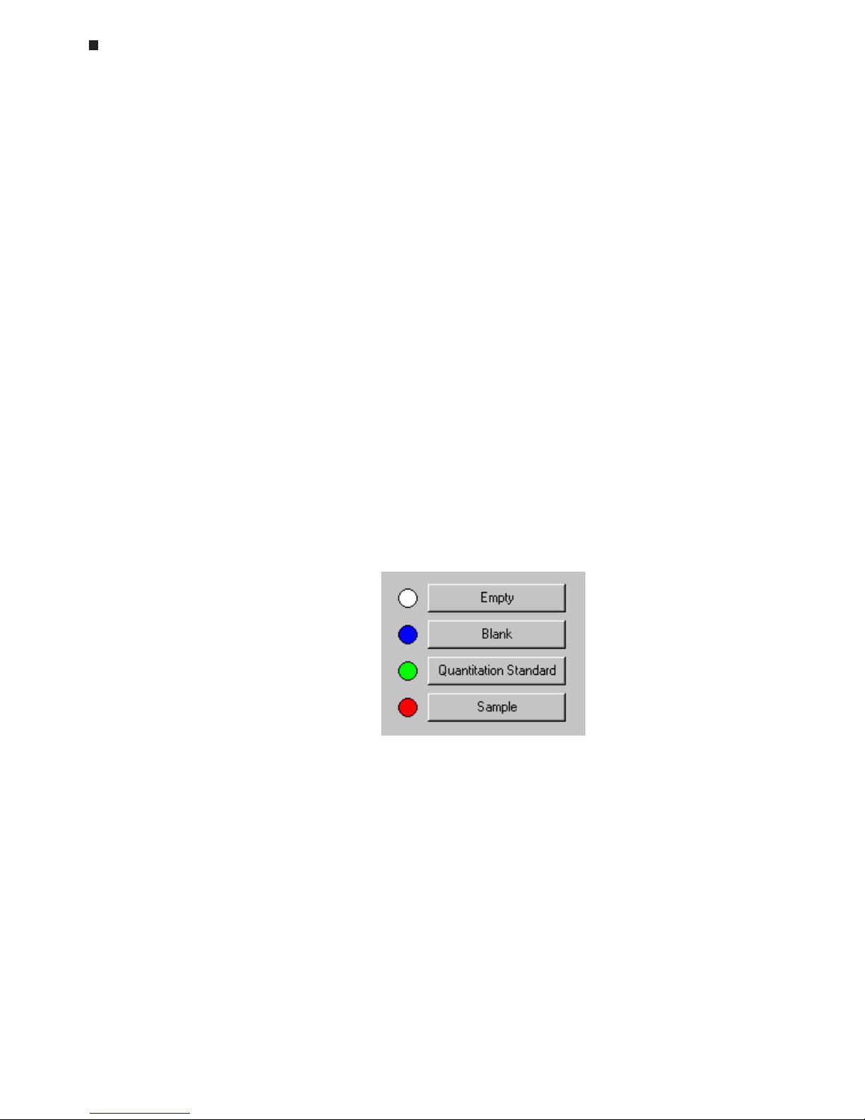
2. Assign the appropriate contents to selected wells by clicking on one of the four
contents buttons:
• Empty (white) – The well is empty. The Opticon™ detector will not measure the
fluorescence in the well. Unspecified wells are considered empty.
• Blank (blue) – The well contains a blank reaction (e.g., buffer only). Fluorescence
intensity measurements from blank wells can be used in background subtraction
calculations.
• Quantitation Standard (green)- The well contains a user-specified standard of
known quantity (see the “Specifying Quantitation Standards” section below).
Fluorescence intensity readings from quantitation standards are used to plot a
standard curve.
• Sample (red) –The well contains an experimental sample (unknown or control).
Page 43

Experimental Setup and Programming
Tech Support: (888) 652-9253 • Sales: (888) 735-8437 • tech@mjr.com • www.mjr.com 6-7
The color of assigned wells in the plate diagram should correspond to the color of the
content specified, and each content assignment should appear in the corresponding
Contents
column of the plate information table.
3. To change the content assignment of a well, select the well as described in step 1,
and click on the desired content button. The well’s color and corresponding content
information in the plate information table will reflect the content change. If a well is
not designated as empty prior to the run, the content assignment for the well can be
changed post run. Changing a "non-empty" well to "empty" post-run will
result in the irreversible loss of fluorescence data for that well.
Specifying Quantitation Standards
If you are using quantitation standards, click the
Specify Quant Standards
button
after you have designated which wells contain standards. A pop-up window will
appear listing all of the wells to which quantitation standards have been assigned.
The scroll bar will become active if the number of standards assigned is greater than
the number that can be displayed in the window.
Enter the quantity of each standard in the
Value
box. Then, specify the
Units
of the
standard by choosing either ng, moles, molecules, ge (genome equivalents), or copies from the pull-down menu, or define your own units by selecting the
Manage
but-
ton. Select
Add
in the Manage Standards window that appears, and type the desired unit designation in the Add Item window that appears. To remove unit designations from the
Units
menu, highlight the designation and click the
Remove
button.
Select
Save
to save the standard specifications, or click
Cancel
to undo any changes
to the standard specifications.
Page 44
6-8 Tech Support: (888) 652-9253 • Sales: (888) 735-8437 • tech@mjr.com • www.mjr.com
Opticon System Operations Manual
A standard curve will be automatically generated using the values supplied during
analysis of the data. You will have the option to adjust the standard curve by deselecting points (see Chapter 8).
Assigning Well Descriptions
To aid in sample identification, you can enter descriptive well labels for individual wells
or groups of wells. Begin by selecting the well(s) using the plate diagram or plate information table as specified in the “Assigning Well Contents” section above. Then, type a
description in the
Well Label
field. The well label will be applied to the selected well or
wells and appear in the Description column in the plate information table. Alternatively,
double click on an individual row in the plate information table and type a well label
directly into the well’s Description field. You can also copy and paste a well label from
one Description field in the table to a second Description field by first double-clicking on
the field and then using either (control c) to copy or (control v) to paste. To simultaneously
paste a well label into the Description fields of multiple wells, select the wells as described
above and use (control v) to paste into the
Well Label
field.
Use the
Clear Well Label
button to delete the well labels for selected wells from the
Description column.
Once you have finished entering plate file parameters, click the
OK
button in the upperleft corner of the plate file window to return to the master file window. A picture and
summary of the assigned plate contents will appear in the Plate Setup section of the master
file window.
Alternatively, if you wish to discard the plate file information and return to the master file,
click
Cancel
.
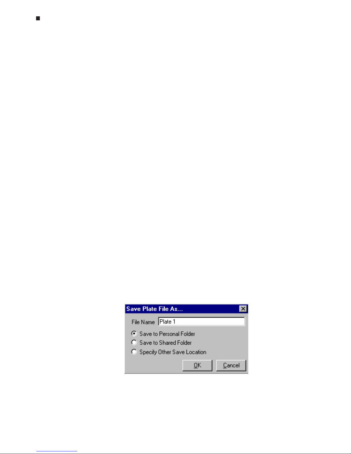
Saving a Plate File
To save the newly created plate file, select the
Save
button from the Plate Setup section in
the master file window. Enter an appropriate name in the
File Name
field of the Save
Plate File As window.
Then, specify the location to which the plate file should be saved. If a specific user has
been designated in the master file window, the plate file may be saved to that user's
personal folder
(Save to Personal Folder)
, to the shared folder (
Save to Shared Folder)
,
or to an alternate location (S
pecify Other Save Location)
. If the designated user is
Shared
,
Page 45

Experimental Setup and Programming
Tech Support: (888) 652-9253 • Sales: (888) 735-8437 • tech@mjr.com • www.mjr.com 6-9
only the last two options are available. If the
Specify Other Save Location
option is cho-
sen, select the
Browse
button to access a standard Windows browse screen, and select
the location to which you wish to save the file.
Creating a Protocol File
A protocol file contains a program that controls the thermal-cycling parameters of a run
and specifies when during the run the Opticon detector will measure the fluorescence in
the wells designated as samples, quantitation standards, and blanks. Protocol steps can
be entered and edited in the protocol file window and a listing and graphical representation of the protocol is displayed for easy review.
Click the
New
button in the
Protocol Setup
section of the master file to create a new pro-
tocol file.
Protocol file window
Insert
protocol
steps
Select methods
of temperature
and lid control
Protocol
listing
Protocol
graphical
representation
Edit
protocol
steps
Page 46

6-10 Tech Support: (888) 652-9253 • Sales: (888) 735-8437 • tech@mjr.com • www.mjr.com
Opticon System Operations Manual
Choosing a Temperature and a Lid Control Mode
Click the
Edit
button in the Temperature and Lid Mode panel to specify the temperature
Control Method and the Lid Control method to be used in the run. The Protocol Options
window will be displayed.
Temperature Control Method
The DNA Engine Opticon system can control block temperature in two different ways,
each of which has implications for the speed and accuracy of sample heating.
1. Calculated Control is the default method of temperature control. Calculated
control is the method of choice for most protocols, yielding consistent, reliable,
and fast programs. When using calculated control, the DNA Engine Opticon
system maintains a running estimate of sample temperatures based on the block’s
thermal profile, the rate of heat transfer through the sample tube, and the sample
volume. Since this estimate is based on known quantities and the laws of thermodynamics, sample temperatures are controlled much more accurately than with
block temperature control.
Hold times can be shortened significantly when protocols are run under calculated control. In addition to the simple convenience of spending less time running
reactions, shorter protocols also help preserve enzyme activity and minimize
false priming. Cycling denaturations run under calculated control are usually
optimal at five to 30 seconds, though optimization of denaturation time may be
beneficial for quantitative protocols. Annealing/extension steps can also be shortened—but the periods for these will be reaction specific.
Calculated control provides for shorter protocols in three ways:
Page 47

Experimental Setup and Programming
Tech Support: (888) 652-9253 • Sales: (888) 735-8437 • tech@mjr.com • www.mjr.com 6-11
• Brief and precise block-temperature overshoots are used to bring samples
to temperature rapidly.
• Incubation periods are timed according to how long the samples, not the
block, reside at the target temperature.
• The instrument automatically compensates for vessel type and reaction
volume.
2. When using Block Control, the DNA Engine Opticon system adjusts the block’s
temperature to maintain the block at programmed temperatures independent of
sample temperature. Block control provides less precision in control of actual
sample temperature than calculated control provides. Under block control, the
temperature of samples always lags behind the temperature of the block. The
length of the time lag depends on the vessel type and sample volume but is
typically between 10 and 30 seconds. Block control is used chiefly to run protocols developed for other thermal cyclers that use block control including the PTC100
®
cycler and the MiniCycler® personal cycler from MJ Research.
Lid Control
When a sample is heated, condensation on the tube cap or the plate cover can occur. This changes the volume of the sample, the concentration of components and thus
the kinetics of the enzymatic reaction. Use of a heated lid minimizes condensation by
keeping the upper surface of the reaction vessel at a temperature slightly greater than
that of the sample itself.
The DNA Engine Opticon system can control lid temperature in three possible ways:
Constant, Tracking
, or
Off
.
• Constant: Keeps the inner lid at a specified temperature (˚C). This is the default
method of control. To use constant lid-temperature control, select
Constant
and
enter a
Lid Temperature
between 30°C and 110°C or use the arrows to scroll to
the desired temperature. A temperature of 5°C to 15°C above the highest temperature in a protocol is recommended. You can also specify a sample-block
temperature below which the heated lid will turn off. Enter a
Lid Shutoff Tempera-
ture
between 1°C and 50°C or use the arrows to scroll to the desired tempera-
ture.
• Tracking: Offsets the temperature of the heated inner lid a minimum specified
number of degrees Celsius in comparison to the temperature of the sample block.
Tracking is useful for protocols with long incubations in the range of 30-70°C,
where it may be undesirable to keep the lid at a very high temperature. An offset
of 5°C above block temperature is adequate for most protocols. To use tracking
lid-temperature control, select
Tracking
and enter the number of degrees, from
1°C to 45°C, the lid temperature should be maintained above the block temperature, using the format
Lid Temperature = Block Temperature +
. You can also use
the arrows to scroll to the desired temperature. To specify a sample-block temperature below which the heated lid will turn off, enter a
Lid Shutoff Temperature
between 1°C and 50°C or use the arrows to scroll to the desired temperature.
Page 48

6-12 Tech Support: (888) 652-9253 • Sales: (888) 735-8437 • tech@mjr.com • www.mjr.com
Opticon System Operations Manual
Note: Because there is no active cooling of the lid, a decrease in the lid temperature may not be observed during rapid cycling. In addition, the lid heats more
slowly than the sample block as a result of its additional thermal mass.
• Off: No power is applied to the heated lid. In this mode, condensation will occur
at a rate consistent with the incubation temperature and the type of tube or plate
sealant being used. This option is recommended only when using an oil or wax
overlay.
Saving Temperature and Lid Control Settings
Click the OK button to apply your temperature and lid control settings to the protocol,
or choose
Cancel
to close the window without changing the settings applied to the
protocol. The settings should appear in the Temperature Control and Lid Settings fields
above the protocol listing and graphical display.
Designing and Entering a Protocol
Programming the DNA Engine Opticon system consists of entering a series of steps encoding a protocol. This section will present a sample protocol and describe how to enter
the protocol steps. Additional protocol options will also be described.
Consider the following example protocol:
1. Incubate at 94°C for 30 seconds
2. Optimize annealing temperature by incubating at a range of 55°C to 65°C across
the 12 columns of the sample block
3. Read the fluorescence intensity of the Blank, Quantitation Standard, and Sample
wells
4. Incubate at 72°C for 1 minute
5. Sequentially repeat steps 1-4, 24 more times, then proceed to step 6
6. Identify and determine the purity of reaction products by melting profile—raise the
temperature from 55°C to 90°C, and read the fluorescence 10 seconds after every
1°C increase in temperature
7. End program
Page 49

Experimental Setup and Programming
Tech Support: (888) 652-9253 • Sales: (888) 735-8437 • tech@mjr.com • www.mjr.com 6-13
Entering a New Protocol
As you insert steps into a protocol, descriptions of the steps will appear in the upper protocol display window and a graphical representation of each step’s temperature and time
period (in minutes) will appear in the lower protocol display window. Use the
Horizontal
Zoom
slider and the scroll bar to clearly view the graphical representation of the protocol.
Before beginning to enter a new protocol, note that the END step is highlighted in the
upper display window. Opticon Monitor software adds new steps before the step that is
highlighted. Protocols are limited to a maximum of 99 steps.
Temperature Step
A temperature step specifies incubation temperature and duration. The DNA Engine
Opticon system ramps the sample to this temperature at its maximum rate—unless
ramp modifying instructions are added to the program (see the “Manual Ramp Rate”
description near the end of this section).
Click the
Temperature
button to enter a temperature incubation step (e.g., step 1 or
step 4 from our example) into a protocol.
Plate read
Melting curve
Page 50

6-14 Tech Support: (888) 652-9253 • Sales: (888) 735-8437 • tech@mjr.com • www.mjr.com
Opticon System Operations Manual
Enter the desired temperature, from 0°C to 105°C, into the
Set Temperature to
field
or use the arrows to scroll to the desired temperature—which is 94°C in step 1 of our
example.
Enter the desired incubation time, to a maximum of 18 hours, in the
Maintain Temp
For
field. Click in the hour: minute: or second field and enter a time period, or use the
arrows to scroll to the desired time—00:00:30 in step 1 of our example. Alternatively, you can select
Forever
to maintain the desired temperature for an infinite period of time. A forever incubation step at the end of a protocol can be useful for holding reaction products at a sub-ambient temperature (we recommend 10°C) until they
can be processed. In the graphical representation of the protocol, a forever incubation is indicated with an .
Click the
Insert
button to add the temperature step to the protocol without further modifications. The temperature step should appear as step 1 in the upper protocol display
window, and a graphical representation of the temperature and duration should appear in the lower window. Note that the END step is again highlighted indicating
that the next step will be added above the END step and therefore after step 1.
You can also choose to modify a temperature step before inserting it into the protocol
by adding options. Available options include:
1. Manual Ramp Rate: Set a slower-than-maximum rate of heating or cooling.
A slower-than-maximum ramp rate ranging from 0.1°C to 2.5°C per second can
be specified. Fast thermal ramping between incubation steps can often help reduce overall reaction times by 10% to 30% and may help reduce production of
non-specific products.
Page 51

Experimental Setup and Programming
Tech Support: (888) 652-9253 • Sales: (888) 735-8437 • tech@mjr.com • www.mjr.com 6-15
2. Increment Temperature: Modifies a temperature step to allow a “per cycle”
increase or decrease of temperature (0.1°C to 10.0°C per cycle) each time the
step is executed. This feature is useful when annealing stringency is a consideration such as in a touchdown program.
In a touchdown program, the annealing temperature begins higher than the calculated temperature, and incrementally decreases each cycle, first reaching, and
eventually falling below the calculated annealing temperature. With the reaction
beginning at a temperature favoring high stringency in hybridization and
incrementing to lower stringency, the higher stringency favors the desired product by creating a high proportion of signal relative to noise in the early amplification cycles.
3. Extend Time: Modifies a temperature step to allow a “per cycle” lengthening
or shortening of a temperature step hold (by 1–60 sec/cycle) each time a step is
executed.
This capability is useful for slowly increasing (typically by 2 to 5 seconds per
cycle) the hold time during an extension step. The number of bases that a polymerase must synthesize during the extension step increases in later cycles because there are more template molecules, because there are fewer active polymerase molecules, or both. The extra time can allow synthesis to be completed.
4. Beep When Completed: Modifies a temperature step so the instrument will
beep when the target temperature is reached.
Gradient Step
The temperature gradient feature allows you to optimize denaturing or annealing
conditions by incubating at several different temperatures simultaneously. For example,
determining the best denaturation temperature may be especially important in optimizing the efficiency of amplification reactions used for quantification. With the MJ
gradient feature, such optimization can be performed in a single experiment. The
range of temperatures that can be achieved from left to right across the 96-well sample
block can be as small as 1°C or as great as 24°C. The maximum programmable
temperature is 105°C; the minimum programmable temperature is 30°C.
Click the
Gradient
button to insert a gradient step into a protocol.
Page 52

6-16 Tech Support: (888) 652-9253 • Sales: (888) 735-8437 • tech@mjr.com • www.mjr.com
Opticon System Operations Manual
The minimum gradient temperature is assigned to the far left column (column #1) of
the sample block and can range from 30°C to 104°C. In the
Set Temperature To
field
in our example, L=55. The maximum gradient temperature is assigned to the far right
column (column #12) and can range from 31°C to 105°C. In the
Set Temperature To
field in our example, R=65. The minimum temperature differential between the far
left and far right columns is 1°C and the maximum differential is 24°C.
After entering the range of temperatures for the gradient, enter the desired incubation time in the
Maintain temperature For
field by clicking in the hour: minute: or second field and entering a time period, or use the arrows to scroll to the desired time—
00:00:30 in step 2 of our example. Alternatively, you can select
Forever
to maintain
the desired temperature for an infinite period of time.
Click
Insert
to add the gradient step to the protocol. The gradient step should appear as step 2 in the protocol display window. Note that the END step is again
highlighted indicating that the next step will be added above the END step and
therefore after step 2.
Page 53

Experimental Setup and Programming
Tech Support: (888) 652-9253 • Sales: (888) 735-8437 • tech@mjr.com • www.mjr.com 6-17
Gradient Calculator
To accurately predict the temperature of each of the twelve columns across the
block during a gradient incubation, select
Gradient Calculator
from the
Tools
menu.
Use the arrows to scroll to the desired left and right column temperatures. Please
note that the gradient temperature distribution is not linear, with a broader spread
in temperature between the center columns of wells. This is a consequence of the
geometry of the Peltier-Joule heaters that underlie the block and is normal. Rest
assured that the temperatures displayed are quite accurate for each well in that
column (± 0.4°C of actual column temperature). The predicted temperature for
the column that yields the best results can then be accurately transferred to a temperature step in a non-gradient protocol.
Plate Read Step
Insertion of a plate read step directs the Opticon detector to measure the fluorescence
of the wells designated as samples, quantitation standards, and blanks. The plate
read begins immediately after the programmed end of the previous incubation step,
step 2 in our example. The Opticon detector performs the plate read at the current
incubation temperature, and then initiates the next step, step 4 in our example.
To insert a plate read step, click the
Plate Read
button. A plate read step will be inserted into the protocol. The plate read step should appear as step 3 in the upper
protocol display window in our example. A plate read appears as an eye icon in the
graphical protocol display. Protocols cannot contain a plate read as a first step.
Adding Multiple Temperature Steps, Gradient Steps, or Plate
Reads
To add additional temperature steps, gradient steps, or plate reads to your protocol, click the appropriate button and follow the directions for the specific step as
outlined above.
Following our example, step 4 is a temperature incubation step of 72°C for a duration of 00:01:00 with no additional options.
Page 54

6-18 Tech Support: (888) 652-9253 • Sales: (888) 735-8437 • tech@mjr.com • www.mjr.com
Opticon System Operations Manual
Goto Step
The goto step allows a protocol of many repeating steps to be shortened. When the
protocol encounters a goto step, it returns to a user-specified step, repeats that step
and all steps that follow back to the goto step. When the protocol has cycled back to
the goto step a specified number of times, the protocol moves on to the step that follows the goto step. Keep in mind that the maximum length of a protocol is 99 steps; a
goto step (regardless of the number of times that a protocol loop will be performed)
counts as only one step.
Step 5 of our example protocol indicates that the protocol should return to step 1,
repeat steps 1-4 24 additional times, for a total of 25 cycles, and then proceed to
step 6. This can be accomplished by including a single goto step.
Click the
Goto
button, and enter the line number of the step to which the protocol
should return. In our example, enter 1 in the
Goto Line
field, and 24 in the
How Many
More Times?
field. Step 5 of our protocol will then direct the protocol to repeat steps
1,2,3, and 4 a total of 24 times before continuing on to step 6.
Click the
Insert
button to add the goto step to the protocol.
Page 55
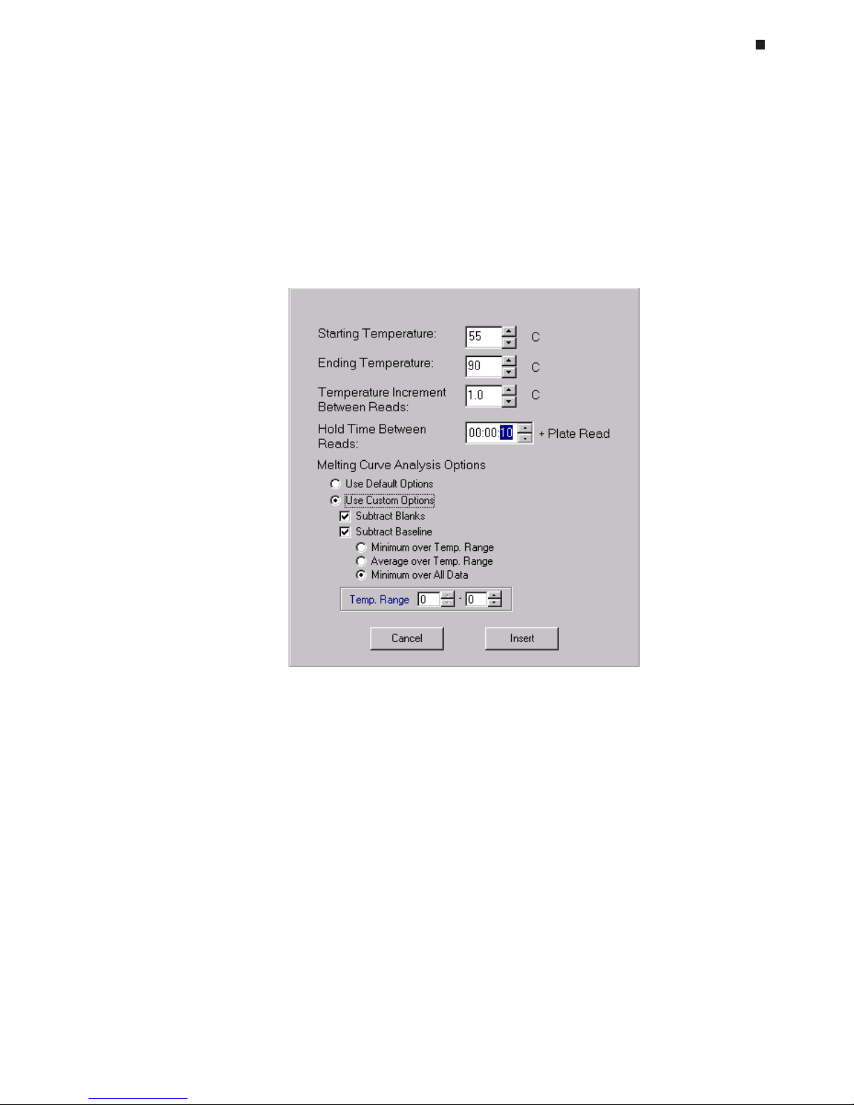
Experimental Setup and Programming
Tech Support: (888) 652-9253 • Sales: (888) 735-8437 • tech@mjr.com • www.mjr.com 6-19
Melting Curve Step
In some instances, such as to verify product identity, you may want to perform a melting curve following a cycling protocol. Melting curve profiles are influenced by several factors including the number and concentration of discreet fragments produced,
the length and G+C content of each fragment, and other factors that influence the
melting temperature of nucleic acids such as buffer conditions.
To add a melting curve step following a cycling protocol, click the
Melting Curve
button.
Enter a
Starting Temperature
(0.0°C to 99.0°C), and an
Ending Temperature
(1.0°C
to 100.0°C).
Next, specify when during the melting curve step the Opticon detector should measure fluorescence. Designate a
Temperature Increment Between Reads
of 0.1°C to
10°C and a
Hold Time Between Reads
(1 second to 1 hour) corresponding to the
duration for which the temperature increment should be maintained before the fluorescence is read. A temperature Increment of 0.2°C and a hold time of 1 second is
recommended for many protocols.
Page 56

6-20 Tech Support: (888) 652-9253 • Sales: (888) 735-8437 • tech@mjr.com • www.mjr.com
Opticon System Operations Manual
Melting Curve Analysis Options can be specified at the time the melting curve step is
created, or analysis options can be altered during analysis of the melting curve data.
See the "Defining Default Data Analysis Options" and "Display" sections in Chapter
8 for an explanation of the available analysis options and information on specifying
default analysis options and altering options during data analysis.
Click the
Insert
button to add a melting curve step to the protocol. Data from only one
melting curve step per protocol can be analyzed.
Editing a Protocol Step
To edit a protocol step, first click on the step to highlight it in the protocol display window.
Then, click the
Edit Step
button. The parameters for the step as it is currently entered will
appear. After making the desired changes, click the
Replace
button to enter the edited
step into the protocol, or click
Cancel
to leave the step unedited.
Deleting a Protocol Step
To delete a protocol step, click on the step to highlight it in the protocol display window.
Then, click the
Delete Step
button to remove the step from the protocol. The remaining
protocol steps will automatically renumber.
Inserting a Protocol Step Between Existing Steps
To insert a protocol step between existing steps, highlight the step in the protocol display
window that will follow immediately after the newly inserted step. All protocol steps are
added immediately before the step that is highlighted in the protocol display window.
Then, click the button corresponding to the type of step you would like to add.
Once you have finished entering protocol file parameters, click the
OK
button in the upper-left corner of the protocol file window to return to the master file window. A graphical
representation of the protocol and a summary of the total number of plate reads, melting
curves, and the estimated run duration will appear in the Protocol Setup section of the
master file window.
Alternatively, if you wish to discard the protocol file information and return to the master
file, click
Cancel
.
Page 57
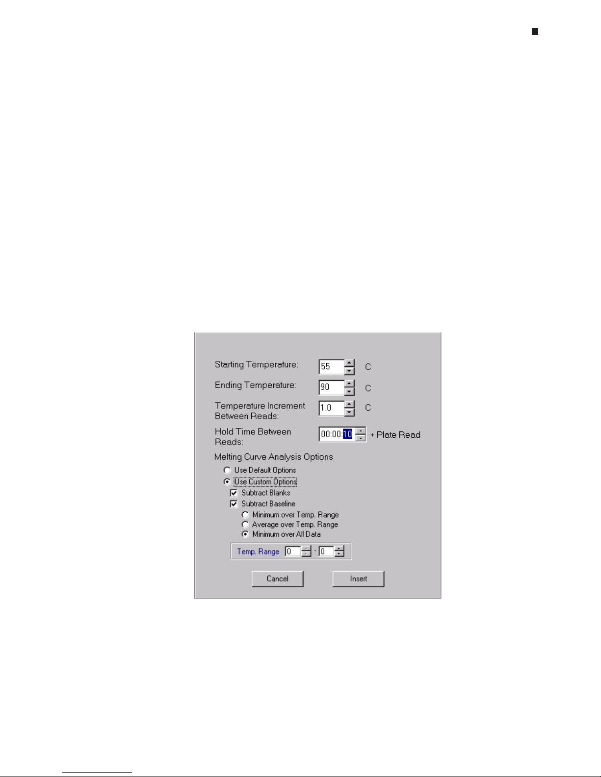
Experimental Setup and Programming
Tech Support: (888) 652-9253 • Sales: (888) 735-8437 • tech@mjr.com • www.mjr.com 6-21
Melting Curve Analysis
A melting curve can be performed to identify specific fragments and/or assess the homogeneity of a sample. Melting curve profiles are influenced by several factors including
the number and concentration of discreet fragments produced, the length and G+C content of each fragment, and other factors that influence the melting temperature of nucleic
acids such as buffer conditions.
The Opticon apparatus can be programmed to run a melting curve independent of a
cycling protocol. This analysis can be useful in a variety of applications including homothermic assays, sizing fragments relative to ladders, and utilizing the 96-well capacity of
the Opticon apparatus to perform endpoint assays to increase throughput.
Melting curves are often useful in verifying the identity of amplification products, as well
as distinguishing positive internal controls from amplified products. In these cases, simply
specify a melting curve after a cycling run, and the instrument will perform both procedures automatically.
To program a melting curve independent of cycling, click the
Melting Curve
button.
Page 58
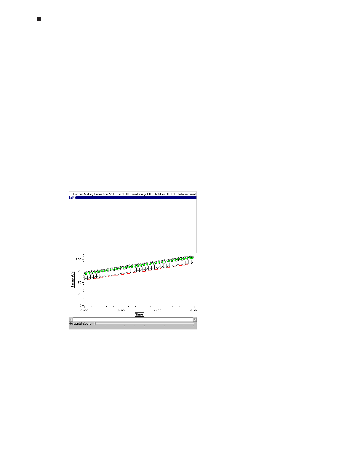
6-22 Tech Support: (888) 652-9253 • Sales: (888) 735-8437 • tech@mjr.com • www.mjr.com
Opticon System Operations Manual
Enter a
Starting Temperature
(0.0°C to 99.0°C), and an
Ending Temperature
(1.0°C to
100.0°C).
Next, specify when during the melting curve step the Opticon detector should measure fluorescence. Designate a
Temperature Increment Between Reads
of 0.1°C to 10°C and a
Hold
Time Between Reads
(1 second to 1 hour) corresponding to the duration for which the temperature increment should be maintained before the fluorescence is read. A temperature
Increment of 0.2°C and a hold time of 1 second is recommended for many protocols.
Melting Curve Analysis Options can be specified at the time the melting curve step is
created, or analysis options can be altered during analysis of the melting curve data. See
the "Defining Default Data Analysis Options" and "Display" sections in Chapter 8 for an
explanation of the available analysis options and information on specifying default analysis
options and altering options during data analysis.
Click the
Insert
button to add a melting curve step to the protocol. Data from only one
melting curve step per protocol can be analyzed.
Page 59

Experimental Setup and Programming
Tech Support: (888) 652-9253 • Sales: (888) 735-8437 • tech@mjr.com • www.mjr.com 6-23
Saving a Protocol File
To save the newly created protocol file, select the
Save
button from the Protocol Setup
section in the master file window. Enter an appropriate name in the
File Name
field of the
Save Protocol File As window. Then, specify the location to which the protocol file should
be saved. If a specific user has been designated in the master file window, the protocol
file may be saved to that user's personal folder
(Save to Personal Folder)
, to the shared
folder (
Save to Shared Folder)
, or to an alternate location (
Specify Other Save Location)
.
If the designated user is
Shared
, only the last two options are available. If the
Specify
Other Save Location
option is chosen, select the
Browse
button to access a standard
Windows browse screen, and select the location to which you wish to save the file.
Saving a Master File
To save a master file, click the
Save
button under Master File. Enter an appropriate name
in the
File Name
field of the Save Master File As window. Then, specify the location to
which the master file should be saved (see the "Saving a Protocol file" section above for
an explanation of location options).
You can also choose to not save this collection of component files and proceed directly to
the run (see Chapter 7 for information on initiating a run).
Assigning Existing Plate and Protocol Files to a Master File
To assign existing plate and protocol files to a new or existing master file, either click the
Open
button in the section of the master file corresponding to the type of file you wish to
assign, or use the Quick Load feature to rapidly assign existing plate/protocol files to a
master file (see the "Using the Quick Load Feature" section below).
Selecting
Open
will display all of the plate/protocol files in either the Shared folder or a
specific user's folder, if a user has been assigned to the master file. Select the desired file
or use the Windows browse screen to locate the file if it has been saved to an alternate
location, and then click
Open
. The plate/protocol file will be applied to the master file
and a corresponding summary will appear in the master file window.
To view the newly assigned plate or protocol file and/or make any necessary modifications, click the
Edit
button in the appropriate section of the master file window. The plate
or protocol file window will open allowing you to modify the file parameters. Select
OK
to retain any modifications and return to the master file window, or select
Cancel
to re-
turn to the master file without modifying the plate/protocol file. Select
Save
to save any
changes to the plate/protocol file under the same or a newly assigned file name. See the
"Saving a Plate/Protocol File" sections in this chapter for additional information on saving plate/protocol files.
Click the
Save
button in the master file section to save any changes to the master file.
Page 60

6-24 Tech Support: (888) 652-9253 • Sales: (888) 735-8437 • tech@mjr.com • www.mjr.com
Opticon System Operations Manual
Reusing Master Files
A new master file need not be created for every run. Existing master files may be reused
without modifying the plate or protocol files, or the master file may be edited to accommodate changes such as a different arrangement of samples in the plate.
If a run has just completed, or a data file for a previously completed run has just been
displayed, and you wish to use the same master file, select the
Repeat This Run
button. To
access a new master file template, select the
Prepare New Run
button. To display an ex-
isting master file, click the
Open
button near the top of the master file window, or use the
Quick Load feature to rapidly assign an existing master file to a master file template (see
the "Using the Quick Load Feature" section below).
Selecting Open will display all of the master files in either the Shared folder, or a specific
user's folder, if a user has been assigned to the master file template. Select the desired
file or use the Windows browse screen to locate the file if it has been saved to an alternate location, and then click
Open
. The master file will be applied to the master file template and the corresponding plate and protocol file summaries will appear in the master
file window.
To use the master file without any changes, proceed to Chapter 7,
Run Initiation and Status
.
You can also modify the master file before initiating a run, by editing the assigned plate
or protocol files (
Edit
button), by substituting files (
Open
button or
Quick Load
), or by
creating new component files (
New
button).
Note: If a component plate or protocol file is edited and saved under the same name,
the edited file will replace the original file in all master files to which that file has been
assigned. Therefore, if you save a master file to your password-protected folder, be sure
that the component plate and protocol files are also saved in your folder. If the component plate and protocol files are not password protected, another user could modify these
files and inadvertently modify your password-protected master file.
Click the
Save
button to save any changes to the master file.
Page 61
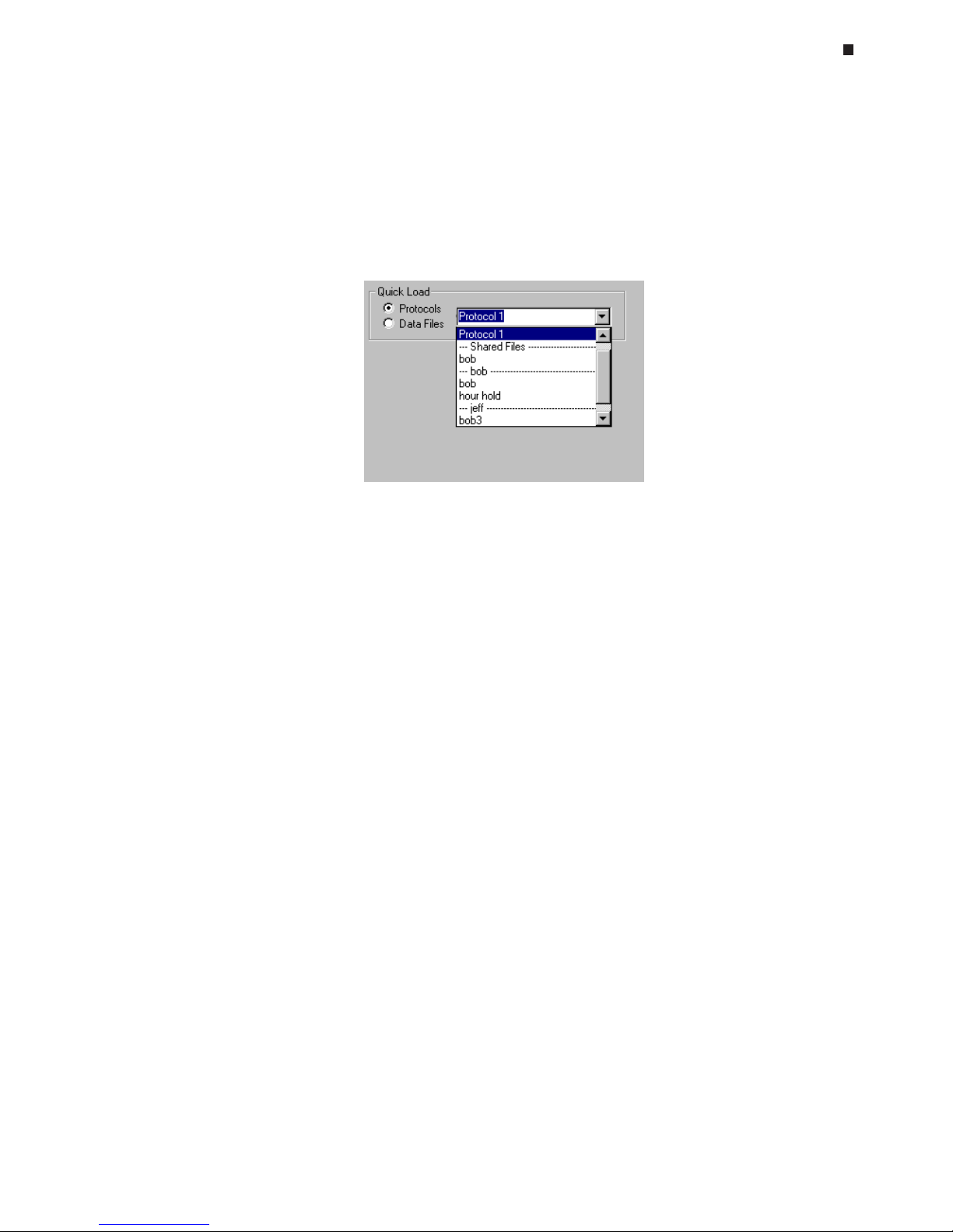
Experimental Setup and Programming
Tech Support: (888) 652-9253 • Sales: (888) 735-8437 • tech@mjr.com • www.mjr.com 6-25
Using the Quick Load Feature
The Quick Load feature can be employed to rapidly access any existing plate, protocol,
master, or data files. If the
Plates/Protocols/Masters
option is selected, all of the available plate, protocol, or master files that have been saved to the Shared folder or individual user folders are displayed in the drop-down menu. The files are listed along with
their associated user as shown below.
Scroll to locate the desired file in the drop-down menu, and select the file. If the
Data Files
option is selected, all of the data files are listed in the drop-down menu. Selecting a data
file will apply the plate, protocol, or master file that was used to generate that data file to
the current master file template.
Page 62

Page 63

7-1
7. Run Initiation and Status
Running a Protocol, 7-2
Monitoring Run Status, 7-2
Protocol Information On the Toolbar, 7-2
The Status Window, 7-3
Thermal Cycler Status, 7-3
Optical Read Status, 7-4
Page 64

7-2 Tech Support: (888) 652-9253 • Sales: (888) 735-8437 • tech@mjr.com • www.mjr.com
Opticon System Operations Manual
Running a Protocol
Before initiating a run, check that the appropriate master file is displayed (see Chapter 6
for instructions on how to create and edit master files).
Initiate the run by clicking the
Run
button on the toolbar. A windows browse screen will
appear asking you to name the file to which the data will be saved. Click
Save
to accept
the default filename consisting of the year, month, day, and six-digit run identification
number (e.g., 20010618_110812), or enter an appropriate filename and then click the
Save
button. The data file will be saved as a .tad (acquired data) file.
Click the
Stop
button on the toolbar to halt the run at any time. The
Skip
button can be
used to skip to the next step in the protocol file.
Monitoring Run Status
Protocol Information On the Toolbar
A summary of run information is displayed at the bottom of the toolbar. This run summary
includes:
• Protocol information: indicates if a protocol or a forever incubation is currently
running.
• Time Remaining: displays an estimate of the time remaining for the run.
• Program Counter: displays the current step and cycle number.
• Temperature: displays the current sample, block, and lid temperatures.
Page 65

Run Initiation and Status
Tech Support: (888) 652-9253 • Sales: (888) 735-8437 • tech@mjr.com • www.mjr.com 7-3
The Status Window
Use the status window to monitor run progress using the thermal cycler status screen, or
monitor real-time data collection using the optical read status screen. The status window
displaying the thermal cycler status screen is automatically displayed when the run is initiated. To access the status window after the run has completed, click the
Status
button on
the toolbar. The tabs in the lower-left corner of the status window toggle the display between
Thermal Cycler Status
and
Optical Read Status
.
Thermal Cycler Status
The run status is graphically displayed in the top portion of the thermal cycler status window. Select the appropriate boxes to display a graph of the sample, block, and/or lid
temperatures over time. The protocol is listed in the bottom portion of the window with
the current step highlighted. The END step is highlighted if the run has finished.
Time slider
Graph selection
bar
Protocol
window
Toggle tabs
Thermal cycler status window
Page 66
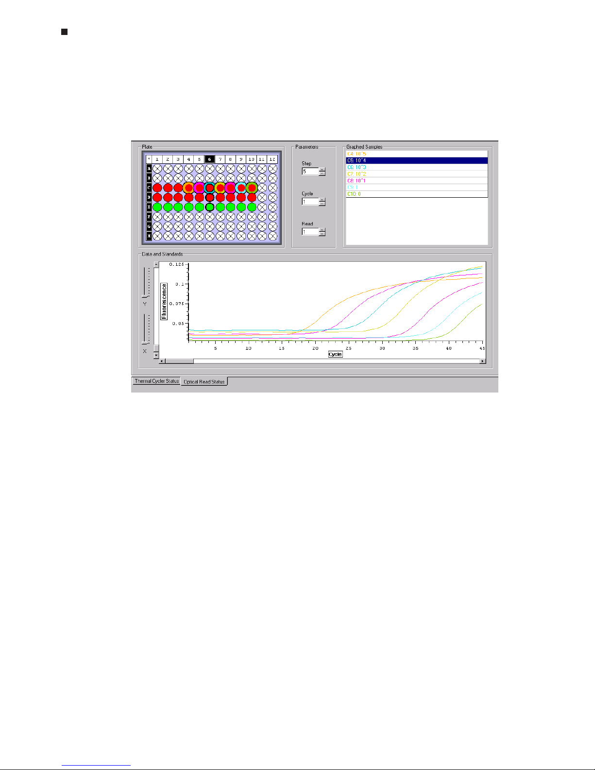
7-4 Tech Support: (888) 652-9253 • Sales: (888) 735-8437 • tech@mjr.com • www.mjr.com
Opticon System Operations Manual
Optical Read Status
Click the
Optical Read Status
tab to monitor real-time data collection.
A graph of Fluorescence versus Cycle number can be displayed for selected wells. Either
raw or normalized data can be displayed depending on the data processing options
specified in the options file. Use the Plate diagram to select the wells to be included in the
Data and Standards graph. See the “Selecting Wells Using the Plate Diagram” section in
Chapter 6 for additional information.
Selected wells will appear outlined in color. The color outlining the well corresponds to
the color of the well coordinates in the Graphed Samples list and to the color of the fluorescence intensity trace in the Data and Standards Graph. The interior color of the well
corresponds to the contents (empty-white, blank-blue, quantitation standard-green, samplered) assigned to the well in the plate file.
Deselect all wells by clicking on any blank area between the wells. To deselect a well or
subset of wells, hold down the control key, and click on the well(s) you wish to deselect.
The well(s) will no longer appear outlined in color, and the corresponding fluorescence
intensity trace will be removed form the graph.
Optical read status window
Page 67

Run Initiation and Status
Tech Support: (888) 652-9253 • Sales: (888) 735-8437 • tech@mjr.com • www.mjr.com 7-5
To highlight the results for a particular sample in the Plate diagram, Data and Standards
graph, and the Graphed Samples list:
• Move the cursor over a well on the Plate diagram. The column number and row letter
coordinates of the well will be highlighted in the Plate diagram, and a well label will
appear displaying the assigned contents and well description. The well will also be
highlighted in the Graphed Samples list, and the trace corresponding to the well will
be thickened in the graph.
• Move the cursor over a particular trace on the graph to thicken the trace and high-
light the corresponding well coordinates in both the Plate diagram and Graphed
Samples list. The x and y coordinates, cycle number and fluorescence intensity, corresponding to the position of the cursor on the trace will also be displayed.
• Select a well from the Graphed Samples list to highlight the well coordinates in the
Plate diagram and thicken the corresponding trace in the graph.
Use the Parameters box to display the signal intensity data for a particular Step, if a plate
read is included in more than one step of the protocol. Use the
Cycle
and
Read
boxes to
highlight the trace for a particular cycle or read number in the Data and Standards graph
with a dotted-vertical line.
Page 68

Page 69

8-1
8. Data Analysis
Quantitation, 8-2
Graphs, 8-3
Using the Plate Diagram to View Fluorescence Intensity, 8-3
Data Graph, 8-4
Adjusting Data Analysis Options, 8-6
Adjusting the Cycle Threshold Line, 8-6
Standards Graph, 8-7
Adjusting the Standard Curve, 8-8
Changing the Values of Quantitation Standards, 8-8
Quantity Calculations, 8-9
Printing and Exporting Quantitation Data, 8-10
Saving the Quantitation Analysis, 8-10
Melting Curve, 8-10
Display, 8-11
Calculations, 8-14
Printing and Exporting Melting Curve Data, 8-15
Saving the Melting Curve Analysis, 8-15
Exporting and Printing Data, 8-15
Exporting Data, 8-15
Copying Data to the Clipboard, 8-16
Printing Data, 8-16
Saving a Data File, 8-17
Defining Default Data Analysis Options, 8-18
Page 70

8-2 Tech Support: (888) 652-9253 • Sales: (888) 735-8437 • tech@mjr.com • www.mjr.com
Opticon System Operations Manual
Quantitation
Continuous, real-time, fluorescence detection of amplification products allows you to accurately calculate the quantity of template initially present in a sample. During the exponential phase of amplification, there is a highly reproducible relationship between the
initial amount of template present in the reaction, and the number of cycles required before a significant increase in fluorescence signal is observed. The larger the initial template number, the fewer cycles required before significant fluorescence signal is detected.
This relationship between starting copy number and the number of cycles preceding detection can be used to calculate the initial quantity of template in a sample. First, the position of the cycle threshold or C(t) line must be defined on a graph of Fluorescence vs.
Cycle number. The C(t) line is often positioned on a graph of baseline-subtracted data
(see the “Defining Default Data Analysis Options” section in this chapter) at a point where
the signals surpass background noise and begin to increase. The threshold cycle for an
individual sample is then defined as the cycle at which the sample’s fluorescence trace
crosses the C(t) line. By including quantitation standards with varying initial amounts of
template in the run, a standard curve of Log Quantity vs. C(T) Cycle can be plotted. The
quantity of initial template in unknown samples can then be calculated by applying the
sample’s threshold cycle to the standard curve. Initially, or for applications requiring a
high degree of precision, including replicate quantitation standards in the run can aid in
positioning the C(t) line. The use of replicates allows you to determine which options for
setting the C(t) line parameters, described below, provide the tightest fit of the replicates
onto the standard curve.
If a run has just completed, or a previously generated data file has been opened by selecting
Open data file
from the
File
menu, click the
Quantitation
button on the toolbar to analyze Data and Standards graphs, adjust the data analysis options, position the cycle-threshold line, adjust the automatically generated standard curve, and calculate the quantity of
sample initially present in a reaction. The Graphs screen is the default quantitation screen.
Page 71

Data Analysis
Tech Support: (888) 652-9253 • Sales: (888) 735-8437 • tech@mjr.com • www.mjr.com 8-3
Graphs
A
Data
graph of Fluorescence (or Log Fluorescence) versus Cycle number, a
Standards
graph of Log Quantity versus C(T) Cycle, or
Both
can be displayed by clicking on the
appropriate tab at the bottom-left side of the quantitation window.
Using the Plate Diagram to View Fluorescence Intensity
The Plate diagram can be useful for selecting wells to include in the Data graph and for
analyzing end-point fluorescence intensity. The interior color of a well in the Plate diagram correlates with the signal intensity measured in the well for the specified
Step, Cycle,
and
Read
number. Dark grey or black wells indicate no or weak signal while white or
light grey wells indicate strong signal.
Page 72
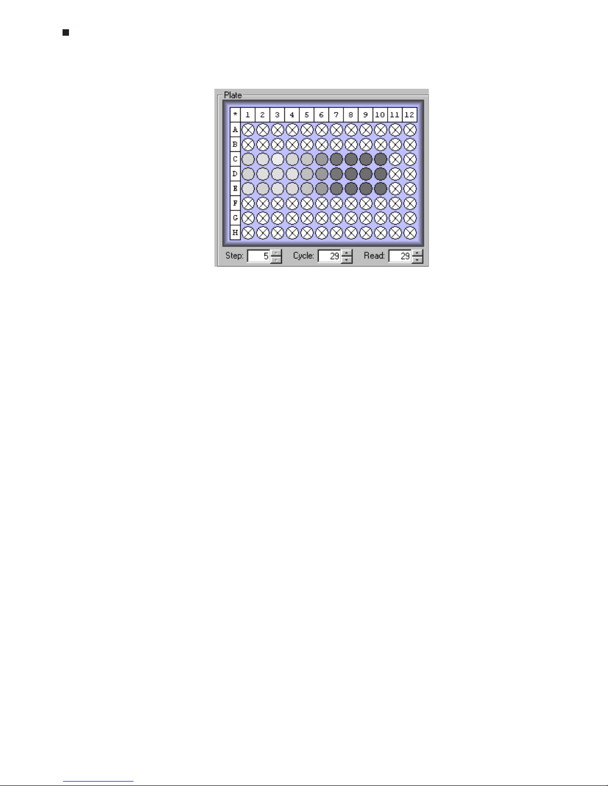
8-4 Tech Support: (888) 652-9253 • Sales: (888) 735-8437 • tech@mjr.com • www.mjr.com
Opticon System Operations Manual
To display the fluorescence data for a particular step, if a plate read is included in more
than one step of the protocol, enter the step number in the
Step
field or use the arrows to
scroll to the desired step. Use the
Cycle
and
Read
boxes to view the signal intensity measured during a specific cycle, or a specific plate read if more than one plate read is included per cycle. You can also use the
Cycle
and
Read
boxes to highlight a particular
cycle or read number in the graph display with a dotted-vertical line.
Data Graph
Use the Plate diagram to select the wells to be included in the Data graph. See the “Selecting Wells Using the Plate Diagram” section in Chapter 6 for additional information.
Selected wells will appear outlined in color. The color outlining the well corresponds to
the color of the well coordinates in the Graphed Samples list and to the color of the fluorescence intensity trace in the Data graph.
Deselect all wells by clicking on any blank area between the wells. To deselect a well or
subset of wells, hold down the control key, and click on the well(s) you wish to deselect.
The well(s) will no longer appear outlined in color, and the corresponding fluorescence
trace will be removed form the graph.
Click the
Data
tab to display a large graph of Fluorescence versus Cycle number. The default data analysis options are used to generate the initial data graph (see the “Defining
Default Data Analysis Options” section for information on setting default analysis options).
Page 73

Data Analysis
Tech Support: (888) 652-9253 • Sales: (888) 735-8437 • tech@mjr.com • www.mjr.com 8-5
To display the log of fluorescence vs. cycle number, select the
Log
option in the lower-left
corner of the graph.
To clearly view regions of the graph, use the X and Y sliders to zoom along the x and y
axes of the graph. The scroll bar can be used to position the region of interest in the
display window. Alternatively, right click and drag the box that appears around the area
of the graph that you wish to magnify.
C(t) line
Page 74

8-6 Tech Support: (888) 652-9253 • Sales: (888) 735-8437 • tech@mjr.com • www.mjr.com
Opticon System Operations Manual
Moving the cursor over the data trace for a well will thicken the trace and display the C(t)
value, along with the x and y coordinates corresponding to the current position of the
cursor over the trace. Moving the cursor over a well in the Plate diagram or selecting a
well in the Graphed Samples list will thicken the trace.
Adjusting Data Analysis Options
After viewing a graph of the fluorescence data versus cycle number, you may wish to
adjust some of the data analysis options. You can adjust the following data analysis options in the quantitation window without altering the default analysis options (see the
“Defining Default Data Analysis Options” section near the end of this chapter for a description of the analysis options and information on altering the default analysis options):
•
Subtract Blanks
•
Subtract Baseline
•
Threshold Cycle
(see “Adjusting the Cycle Threshold Line” immediately below)
Adjusting the Cycle Threshold Line
The C(t) (cycle threshold) line appears as a dotted horizontal line on the Data graph at a
position specified in the default data analysis options. To readjust the position of the C(t)
line, select one of the
Threshold
options, or click and drag the C(t) line on the graph to
the desired position. The C(t) line is often positioned such that the C(t) line intersects the
fluorescence traces, on a graph of baseline-subtracted data, at a point where the signals
surpass background noise and begin to increase. If no C(t) line appears on the Data
graph, select
Manual
from the
Threshold
options and enter a value for the C(t) line less
than the maximum fluorescence value displayed on the y-axis of the graph. Then, click
and drag the C(t) line to the desired position.
Options for setting the C(t) line include:
• Manual: The C(t) line can be set manually by entering a threshold value for fluores-
cence intensity between 0-10, or by dragging the C(t) line to the desired position on
the graph.
C(t) line
Page 75

Data Analysis
Tech Support: (888) 652-9253 • Sales: (888) 735-8437 • tech@mjr.com • www.mjr.com 8-7
• Standard Deviation over Cycle Range: The C(t) line can be automatically set to
a multiple of standard deviations above the mean where the multiple and the cycle
range are specified by the user. Enter the desired cycle range in the
Cycle Range
boxes, and enter the multiple in the
Standard Deviation over Cycle Range X
box. The
Cycle Range
settings are applied to both the Threshold and Subtract Baseline func-
tions.
It is often useful to display both the Data and the Standards graphs when establishing the
position of the C(t) line. The best option for setting the C(t) line can often be determined
by observing the effects of each option on the fit of the quantitation standards to a linear
standard curve. The effect of the position of the C(t) line on the standard curve can easily
be visualized by displaying both graphs and dragging the C(t) line up and down.
In establishing the position of the C(t) line, it may also be helpful to display the log of
fluorescence vs. cycle number by selecting the
Log
option in the lower-left corner of the
graph window. Often, the C(t) line can be set at a lower position upon examination of
the log graph.
Standards Graph
Click the
Standards
tab to display a large Standards graph.
Page 76

8-8 Tech Support: (888) 652-9253 • Sales: (888) 735-8437 • tech@mjr.com • www.mjr.com
Opticon System Operations Manual
A standard curve is automatically generated using the information that was provided in
the Specify Quantitation Standards window during creation of the plate file. The Standards Graph displays the base-10 logarithm of initial quantity (ng, moles, molecules,
genome equivalents, copies, or user-defined units) versus the C(T) Cycle, the cycle number at which the intensity trace intersects the C(t) line. The equation describing the linear
standard curve is displayed in the form y = mx + b where m = the slope of the line and b
= the y-intercept. The R-square (R^2) value indicates how well the fit of the standard curve
describes the variation in the data. The value of R-square can vary between 0 and 1,
with values closer to 1 signifying a good fit. An R-square value of 0.999 indicates that
the fit of the linear standard curve explains 99.9% of the variation in the data.
Select the
Show selected wells
option to apply the Graphed Samples to the standard curve.
The samples will appear as gray dots while the standards appear as black dots.
If a Standards graph is not automatically displayed, check that the C(t) line has been
appropriately set on the Data graph, and that the quantitation standards have been defined in the Specify Quant Standards window (see the “Changing the Values of Quantitation
Standards” section below).
Adjusting the Standard Curve
If desired, you can adjust the standard curve by deselecting outlying points. Moving the
cursor over a data point will increase the size of the point and highlight the corresponding well in the plate diagram, Graphed Samples list, and Data graph. To exclude a point
from the standard curve, click on the point and it will turn red indicating that it is no longer
being used in the calculation of the curve. The standard curve will be automatically replotted to exclude the deselected point.
If multiple sets of standards have been included in a single run, points may be excluded
such that the standard curves of interest are serially displayed. Recall that only the black
(selected) standards are used in quantity calculations and only these standards will appear when the graph is printed.
Changing the Values of Quantitation Standards
If, during creation of the plate file, a mistake was made in entering the values of quantitation standards, or quantitation standards were not specified, it is possible to change or
add quantitation standards during the data analysis phase. To access the Specify Quant
Standards window, select
Plate Setup
from the
View
menu, and then click the
Specify
Quant Standards
button. Enter the value and units of each standard and then click the
OK
button. Save the changes to the plate file, and then click the
Quantitation
button on
the toolbar to continue analyzing data with the modified standards.
Page 77
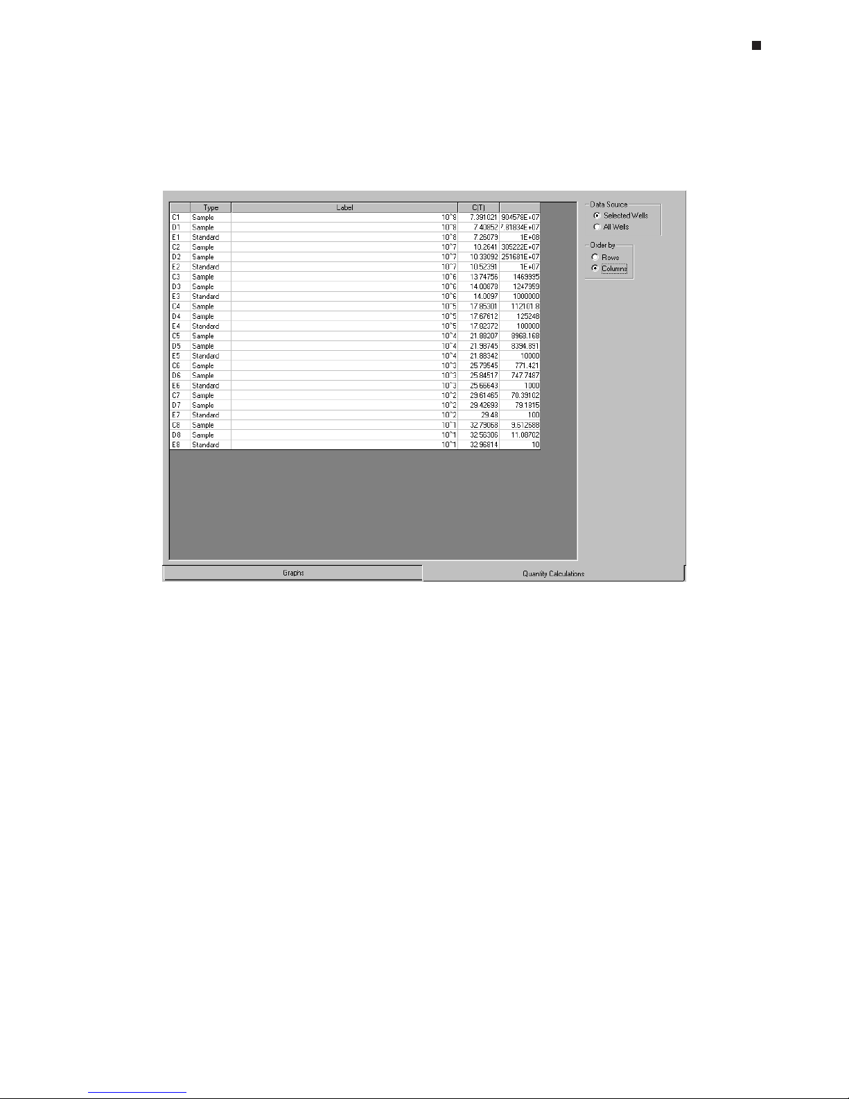
Data Analysis
Tech Support: (888) 652-9253 • Sales: (888) 735-8437 • tech@mjr.com • www.mjr.com 8-9
Quantity Calculations
Click the
Quantity Calculations
tab to display the quantity calculations window.
The Quantity Calculations table lists:
•
Well
coordinates
• The
Type
of well contents
• A descriptive well
Label
(if specified)
• The
C(T)
value, the cycle number at which the fluorescence intensity trace for a well
intersects the C(t) line on the Data graph.
• The initial quantity of template calculated to be present in the reaction. This can be
expressed in several different units including ng, ge (genome equivalents), moles,
molecules, copies, or user-defined units.
To view the quantity calculations for only those wells selected in the plate diagram, choose
the
Selected Wells
option in the Data Source box. To view the quantity calculations for all
non-empty wells, choose the
All Wells
option in the Data Source box.
To display the quantity calculations in order by rows (A1-A12, B1-B12, etc.), choose the
Rows
option in the Order by box. To display the quantity calculations in order by col-
umns (A1, B1, C1, D1, etc.), choose the
Columns
option in the Order by box.
Page 78

8-10 Tech Support: (888) 652-9253 • Sales: (888) 735-8437 • tech@mjr.com • www.mjr.com
Opticon System Operations Manual
Printing and Exporting Quantitation Data
For information on printing and exporting quantitation data, refer to the “Printing and
Exporting Data” section near the end of this chapter.
Saving the Quantitation Analysis
See the “Saving a Data File” section below for information on saving a data file with the
applied analysis options.
Melting Curve
Performing a melting curve analysis following amplification can aid in product identification and determination of product homogeneity, often eliminating the need for timeconsuming electrophoresis. If a chemistry’s fluorescence is dependent on annealing, a
decrease in fluorescence is observed as melting progresses. Because the melting temperature of nucleic acids is affected by length, G+C content and the presence of base
mismatches among other factors, products can often be distinguished by their melting
characteristics.
If a run has just completed, or a previously generated data file has been opened by selecting
Open data file
from the
File
menu, click the
Melting Curve
button on the toolbar
to analyze melting curve data.
Page 79

Data Analysis
Tech Support: (888) 652-9253 • Sales: (888) 735-8437 • tech@mjr.com • www.mjr.com 8-11
Display
The Display screen is the default screen in the melting curve analysis window.
A graph of Fluorescence versus Temperature, -dI/dT versus Temperature, or both can be
displayed for selected wells.
1. Use the Plate diagram to select the wells to be included in the graph. See the “Selecting
Wells Using the Plate Diagram” section in Chapter 6 for additional information.
Deselect all wells by clicking on any blank area between the wells. To deselect a well or
subset of wells, hold down the control key, and click on the well(s) you wish to deselect.
The well(s) will no longer appear outlined in color, and the corresponding trace(s) will be
removed form the graph.
Selected wells appear outlined in color. The color outlining the well corresponds to the
color of the well coordinates in the Graphed Samples list and to the color of the trace in
the melting curve graph.
Tm (-dI/dT max)
dI/dT
FWHM
Intensity
-dI/dT
Page 80

8-12 Tech Support: (888) 652-9253 • Sales: (888) 735-8437 • tech@mjr.com • www.mjr.com
Opticon System Operations Manual
2. Use the
Display
panel to choose how the melting curve data is graphed.
• Select
Intensity
to graph Fluorescence intensity versus Temperature.
• Select
-dI/dT
to graph the negative first derivative of the fluorescence intensity versus
Temperature. The dotted vertical line, drawn in the same color as the corresponding
trace, marks the maximum -dI/dT value, the temperature at which the rate of change
in fluorescence is the greatest. This corresponds to the melting temperature (Tm) of
the product. The dotted horizontal line indicates the sharpness of the -dI/dT curve as
the number of degrees Celsius over which the curve spans (i.e., the curve width) at
half of the maximum -dI/dT value calculated for the well.
• Select both
Intensity
and
-dI/dT
to simultaneously display the Intensity and the -dI/dT
graphs.
• Select
Show Relative Intensities
to display the relative intensities of the signals for the
selected wells. Deselect this option to autoscale each trace on the graph.
3. After viewing a graph of the Fluorescence data versus Temperature, you may wish to
adjust some of the data analysis options initially specified in the creation of the melting
curve step or in the default analysis options. You can adjust the following data analysis
options in the melting curve window without altering the default analysis options (see the
“Defining Default Data Analysis Options” section for a description of the analysis options
and information on altering the default analysis options):
•
Subtract Blanks
•
Subtract Baseline
Page 81

Data Analysis
Tech Support: (888) 652-9253 • Sales: (888) 735-8437 • tech@mjr.com • www.mjr.com 8-13
Note: If
Minimum over Temp. Range
or
Average over Temp. Range
is selected
as the
Subtract Baseline
option, and the
Temp. Range
values are altered, select
the reload button to redraw the melting curve graph applying the new baseline
temperatures.
4. The Temperature Cursor controls can be used to highlight the results associated with
a particular temperature by drawing a dotted vertical line on the graph at the designated
temperature. Either use the scroll bar to scroll to the desired temperature, or enter the
desired temperature in the box located to the right of the scroll bar.
5. The Peak Location Boundaries box allows you to limit the area in which -dI/dT
peaks are found and used to calculate melting temperatures. This can be particularly
useful for excluding unwanted peaks, or determining the melting temperature, Tm (-dI/dT
maximum), for a second, smaller peak (e.g., genotyping heterozygotes). You can set left
and right peak location boundaries by entering the temperature or by using the arrows to
scroll to the desired temperature. Alternatively, drag the peak location boundary guides
to the desired location on the graph.
6. The Point Smooth slider allows you to change the number of points that are included
in calculating the smoothing of the melting curve graph. This can be particularly useful
for resolving peaks when many reads have been collected over small intervals in temperature resulting in a choppy graph. The default for well-resolved data is a setting of 3.
Without peak location boundaries
Note that the Tm
(-dI/dT max)
is now calculated for
the smaller peak
With peak location boundaries
reload
Page 82

8-14 Tech Support: (888) 652-9253 • Sales: (888) 735-8437 • tech@mjr.com • www.mjr.com
Opticon System Operations Manual
Calculations
Click on the
Calculations
tab at the bottom of the melting curve window to display the
melting curve calculations screen.
The Calculations table lists:
•
Well
coordinates.
• The
Type
of well contents.
• A descriptive well
Label,
if entered during creation of the plate file.
•
Tm (-dI/dT Max)
: The melting temperature (Tm), the temperature at which -dI/dT is at
the maximum value calculated for the well.
•
dI/dT FWHM (Full Width Half Maximum)
: Describes the sharpness of the -dI/dT
curve as the number of degrees Celsius over which the curve spans, i.e., the curve
width, at half of the maximum -dI/dT value calculated for the well.
To view the melting curve calculations for only those wells selected in the plate diagram,
choose the
Selected Wells
option in the Data Source box. To view the calculations for all
non-empty wells, choose the
All Wells
option in the Data Source box.
Page 83

Data Analysis
Tech Support: (888) 652-9253 • Sales: (888) 735-8437 • tech@mjr.com • www.mjr.com 8-15
To display the calculations in order by rows (A1-A12, B1-B12, etc.), choose the
Rows
option in the Order by box. To display the calculations in order by columns (A1,B1, C1,
D1, etc.), choose the
Columns
option in the Order by box.
Printing and Exporting Melting Curve Data
For information on printing and exporting melting curve data, refer to the “Printing and
Exporting Data” section below.
Saving the Melting Curve Analysis
See the “Saving a Data File” section below for information on saving a data file with the
applied analysis options.
Exporting and Printing Data
Exporting Data
For customized data analysis, Opticon Monitor™ software provides the option to write
the fluorescence data collected during the run, along with the protocol and run parameters, to either an Excel or CSV (comma separated values) file. Select
Export
from either
the
Quantitation
or
Melting Curve
pull-down menu, and select
Excel
or
CSV
.
If the Excel option is chosen, the processed
Data
, either quantitation or melting curve
data, for the currently displayed step, along with the
Analysis Options, Protocol
and
Plate
summaries will be written to the Excel compatible file. The Excel export options can not
be customized. In the
Export Options
window, select OK and type an appropriate file
name in the Windows browse screen that appears, if the default name, data file
name_platereads is not acceptable. The Excel compatible file will be saved as an .xls file
in the Opticon Monitor data folder unless an alternate file location is specified.
Note: Excel 2000 must be installed on the computer in order to use the Export Excel
option.
If the CSV option is chosen, the export options can be customized. Select
Data
to export
the fluorescence values measured in either all steps of the protocol (
All Run Data
), or the
values from the
Currently Displayed Step Only
. Then, specify if the
Raw, Normalized,
or
Processed
fluorescence values should be exported. The Raw option will export the fluorescence values measured by the Opticon™ detector with no data processing. The Normalized option will export fluorescence values normalized to account for any variation in
signal measurement between wells by applying a normalization constant to the data collected in each well. These constants are calculated by subtracting the signals obtained
when no plate is present in the instrument from signals obtained with a plate of uniform
fluorescence. The Processed option exports fluorescence values from which blanks and/
or a baseline value have been subtracted from the normalized data.
Page 84

8-16 Tech Support: (888) 652-9253 • Sales: (888) 735-8437 • tech@mjr.com • www.mjr.com
Opticon System Operations Manual
Select
Analysis Options
to include a summary of the analysis options applied to the data
including whether blanks were subtracted and the method of baseline subtraction, if any.
Select
Protocol
to include a summary of the protocol used to generate the data. Select
Plate
to include a summary of the plate file information including the well contents and
any well descriptions.
After choosing the desired export options for the CSV file, click
OK
to display a Windows browse screen allowing you to enter a file name and specify a location in which to
save the file.
Copying Data to the Clipboard
From the quantitation window, you have the option to copy the Data Graph, Standards
Graph, and Quantity Calculations to the clipboard for pasting into word processing or spread
sheet programs. From the melting curve window, the Data Graph and Calculations can be
copied to the clipboard. Select
Copy to Clipboard
from either the
Quantitation
or
Melting
Curve
pull-down menu, and then select the desired graph or calculations option.
Printing Data
To print quantitation or melting curve analysis graphs and calculations, select
Print
from
the
File
menu while in the appropriate data analysis window. Select
Print Preview
from
the
File
menu to view the data in the form in which it will be printed.
Page 85

Data Analysis
Tech Support: (888) 652-9253 • Sales: (888) 735-8437 • tech@mjr.com • www.mjr.com 8-17
Saving a Data File
To save analyzed data, which could include the samples graphed, the analysis option
settings, the position of the C(t) line, a standards graph including any deselected points,
and/or a melting curve graph including peak location boundaries and display options,
select
Save data file
or
Save data file as
from the
File
pull-down menu.
Page 86
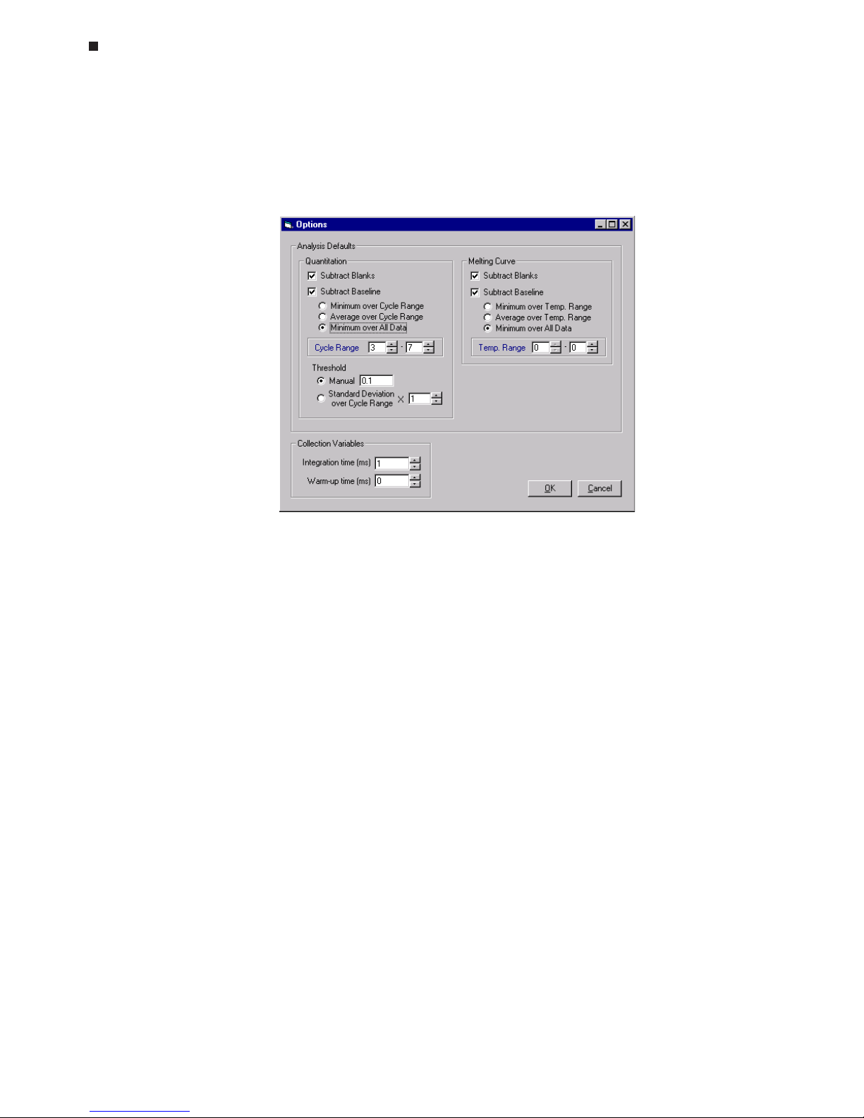
8-18 Tech Support: (888) 652-9253 • Sales: (888) 735-8437 • tech@mjr.com • www.mjr.com
Opticon System Operations Manual
Defining Default Data Analysis Options
To define the default options for data analysis, select
Options
from the
Tools
pull-down
menu.
The
Analysis Defaults
are set separately for
Quantitation
and
Melting Curve
data. Data
analysis options include:
• Subtract Blanks: If this option is selected, the fluorescence measured in all wells
designated as blanks (blue) will be averaged and subtracted, as background, from
the fluorescence measured in all wells designated as samples (red) or quantitation
standards (green).
• Subtract Baseline: If this option is selected, the baseline signal, an absolute fluo-
rescence value, will be subtracted from the fluorescence data collected in each well.
This value is calculated based on the signals measured in each well and thus will
vary from well to well.
There are three options for defining the baseline signal value for a well:
•
Minimum over all Data
: The baseline signal is defined as the weakest fluores-
cence signal measured in the well. This value will be set to zero.
•
Average over Cycle Range (Temp Range)
: The baseline signal value is defined as
the average of the measured fluorescence calculated from a specified range of
cycles (quantitation data) or temperatures (melting curve data).
•
Minimum over Cycle Range (Temp Range)
: The baseline signal value is defined
as the minimum fluorescence value measured in a specified range of cycles (quantitation data) or temperatures (melting curve data).
Page 87

Data Analysis
Tech Support: (888) 652-9253 • Sales: (888) 735-8437 • tech@mjr.com • www.mjr.com 8-19
• Threshold Cycle (Quantitation only): This quantitation option positions the
C(t) (cycle threshold) line for use in quantitation of starting copy number. The C(t)
line is often positioned on a graph of baseline-subtracted data at a point where
the signals surpass background noise and begin to increase (see the “Quantitation” theory on page 8-2).
There are two options for setting the cycle threshold line:
•
Manual
: The C(t) (cycle threshold) line can be set manually by entering a
threshold value for fluorescence intensity between 0-10 on the y-axis.
•
Standard Deviation over Cycle Range:
The C(t) line can be automatically
set to a multiple of standard deviations above the mean where the multiple and the cycle range are specified by the user. Enter the desired cycle
range in the
Cycle Range
boxes, and enter the multiple in the
Standard
Deviation over Cycle Range X
box. The
Cycle Range
settings are applied
to both the Threshold and Subtract Baseline functions.
Setting the C(t) position in the default options prior to a run is particularly useful
when using an established set of reaction conditions. When using new chemistries or changing reaction conditions, it is often desirable to reposition the C(t)
line in the Quantitation window by clicking and dragging the C(t) line on the
Data and Standards graph or by using the Threshold options in the quantitation
window (see the “Adjusting the Cycle Threshold Line” section in this chapter).
Note: Refer to the “Running a Protocol” section in Chapter 7 for information on
setting the
Collection Variables
.
After you have completed defining the Analysis Defaults, select
OK
to save your
changes and return to the previously displayed setup or analysis screen.
Page 88

Page 89

9-1
9. Maintenance
Cleaning the DNA Engine Opticon, 9-2
Cleaning the Chassis and Block, 9-2
Cleaning the Air Vents, 9-2
Cleaning the Optics, 9-2
Changing the Fuses, 9-3
Page 90

9-2 Tech Support: (888) 652-9253 • Sales: (888) 735-8437 • tech@mjr.com • www.mjr.com
Opticon System Operations Manual
Cleaning the DNA Engine Opticon® Unit
Cleaning the Chassis and Block
Clean the outside of the DNA Engine Opticon unit with a damp, soft cloth or tissue whenever something has been spilled on it, or when the chassis is dusty. A mild soap solution
may be used if needed.
Clean block wells with swabs moistened with water, 95% ethanol, or a 1:100 dilution of
bleach in water. If using bleach, swab wells with water afterward to remove all traces of
bleach. Clean spilled liquids out of the block as soon as possible; dried fluids can be difficult to remove. Do not clean the block with caustic or strongly alkaline solutions (e.g., strong
soaps, ammonia, or bleach at a higher concentration than specified above). These will
damage the block’s protective anodized coating, and possibly lead to electrical shorting.
Caution: Do not pour any cleaning solution into the block’s wells and then
heat the block, in an attempt to clean it. Severe damage to the
block, the heated lid, and the chassis can result.
Cleaning the Air Vents
With the Opticon™ unit turned off, clean the air intake and exhaust vents with a soft-bristle
brush, a damp cloth, or a vacuum cleaner whenever dust is visible (see figure 2-1). If
these vents become clogged with dust and debris, airflow to the heat sink is hampered,
causing performance problems related to overheating.
Tip: To prevent problems with overheating, check regularly for dust buildup.
Cleaning the Optics
The optical components of the detector should not be cleaned by the user. Disassembly of
the optical tower will void your warranty.
Should you suspect difficulty with the optics, please contact the customer service staff of
MJ Research, Inc. or one of its distributors.
Page 91

Maintenance
Tech Support: (888) 652-9253 • Sales: (888) 735-8437 • tech@mjr.com • www.mjr.com 9-3
Changing the Fuses
The circuits in the DNA Engine Opticon unit are protected by four fuses, two external,
user-changeable 6.3A, 250V Type S505, fast acting, 5 x 20mm fuses and two user-inaccessible 8A fuses. When a fuse blows, an error message will appear in the Opticon
Monitor™ software indicating that it can not communicate with the instrument.
Warning: The DNA Engine Opticon unit incorporates neutral fusing, which
means that live power may still be available inside the unit even
when a fuse has blown or been removed. Never disassemble the
thermal cycler base. You could receive a serious electrical shock.
Disassembling the base will also void your warranty.
To change the 6.3A fuses:
1. Disconnect the power cord from the back of the instrument. Move the power switch to
the “0” (off) position.
2. Turn the computer off, and disconnect the serial and DAQ cables from the Opticon
unit. The Opticon unit also draws power from the computer.
3. Insert one corner of a small flat-head screwdriver just under the fuse plug, located
immediately below the power switch and just above the power cord jack, and gently
pry the plug loose. Pull the plug straight out as far as it will go, then push it downward to expose the 6.3A fuses.
4. Remove both fuses and replace with new ones (it is impossible to visually determine
which fuse is blown). You may also test the fuses with an ohmmeter to determine
which is defective and replace just that one.
5. Gently press the fuse cover back in place, and reconnect the power cord and the
computer.
6. Once the fuse has been replaced and the power restored, the DNA Engine Opticon
unit will resume the run, but will not communicate with the Opticon Monitor software.
Restart the software to halt the run as no data will be collected.
Page 92

Page 93

10-1
10. Troubleshooting
Calibration, 10-2
Testing Calibration, 10-2
Recalibrating, 10-2
Software Error Messages, 10-3
Page 94

10-2 Tech Support: (888) 652-9253 • Sales: (888) 735-8437 • info@mjr.com • www.mjr.com
Opticon System Operations Manual
Calibration
The Opticon™ detector is calibrated at the factory and this calibration will accommodate
most applications. If you wish to reload the factory default calibration after manually
recalibrating the instrument, select
Restore Factory Calibration
from the
Tools
menu.
Testing Calibration
An accurately calibrated instrument will detect the same fluorescence intensity in every
well when reading samples of uniform composition.
To determine if the Opticon detector is accurately calibrated:
1. Prepare a test plate by accurately pipetting 50µl of a carefully-prepared 500nM
fluorescein solution into each of the 96 wells of a microplate.
2. Program the following protocol:
• Temperature step of 30°C for 30 seconds
• Plate Read step
• Goto line 1 for a total of 2 more times
• End.
3. Analyze the fluorescence data for all 96 wells using the Optical Read Status screen.
If the instrument is accurately calibrated, the fluorescence data should appear as
relatively straight lines that are tightly clustered—within the accuracy of pipetting.
Several test plates should be measured to determine the error resulting from pipetting.
4. If the fluorescence data do not appear as tightly-clustered straight lines, follow the
instructions below for recalibrating the instrument.
Recalibrating
1. Select
Calibrate Instrument
from the
Tools
menu.
2. Remove the plate from the cycler block, if present, when instructed by the software to
do so.
3. Insert a calibration plate when instructed. (Prepare a calibration plate by accurately
pipetting 50µl of a carefully-prepared 500nM fluorescein solution into each of the
96 wells of a microplate.)
4. Rotate the plate 180° when instructed.
The instrument is now calibrated.
Page 95

Troubleshooting
Tech Support: (888) 652-9253 • Sales: (888) 735-8437 • tech@mjr.com • www.mjr.com 10-3
Software Error Messages
The following tables list software error messages along with their probable causes and
suggested resolutions. For help resolving software problems or for additional information, contact MJ Research technical support at 888-652-9253 (in the US or Canada) or
contact your local distributor (outside the US or Canada).
egasseMrorrEesuaCnoituloseR
atanurtsumrotinoMnocitpO
tsaeltafonoituloserneercs
tsujdaesaelP.867x4201
tratserdnanoituloserruoy
.rotino
MnocitpO
retupmocehtfonoituloserehT
.woloottessirotinom
dnanoituloserehtesaercnI
rotinoMnocitpOehttratser
.erawtfos
dnift'ndluocrotinoMnocitpO
/smron(selifatadtnatropmi
JMruoytcatnocesaelP.)seorez
uoY.plehrofevi
tatneserpeR
dnasnurputesotelbaeblliw
tontubsnurdetelpmocweiv
.devlosersisihtlitnusnurtrats
tondluocelifno
itazilamronehT
ehtgnidaoldnadesseccaeb
.deliafsrotcafnoitazilamron
ybtnemurtsniehtetarbilaceR
gnisoohc
tnemurtsnIetarbilaC
ehtmorf
slooT
ehtfI.unem
JMtcatnoc,stsisrepmelborp
.cnI,hcraeseR
dnift'ndluocrotinoMnocitpO
.)niag(selifatadtnatropmi
JM
ruoytcatnocesaelP
uoY.plehrofevitatneserpeR
dnasnurputesotelbaeblliw
tontubsnurdetelpmocweiv
.devlosersis
ihtlitnusnurtrats
erawtfosrotinoMnocitpO
,elifniagehtdaoltondluoc
nocitpo\selifmargorp\:c
.xdi.niag\rotin
om
.cnI,hcraeseRJMtcatnoC
nigninnursirotinoMnocitpO
!edoMylnOnoitazilausiV
nocitpOfoypocrehtonA
dnagninnur
sierawtfosrotinoM
sseccaevisulcxesahypoctaht
.secafretnitnemurtsniehtot
nocitpOfoypocsihttixE)1
ehtesudna
erawtfosrotinoM
ypocrehtonafI)2.ypocrehto
tih,gninnurt'nsi
,>ETELED<>TLA<>LRTC<
,reganamksatehtesoohc
,bat
sessecorpehtesoohc
,emanegamikcilc
,exe.rotinomnocitpootog
dneesoohcdna,kcilcthgir
detsilllarofsihtoD.sse
corp
egamiexe.rotinoMnocitpO
.seman
Page 96

10-4 Tech Support: (888) 652-9253 • Sales: (888) 735-8437 • info@mjr.com • www.mjr.com
Opticon System Operations Manual
egasseMrorrEesuaCnoituloseR
.tneserptnemurtsnionsierehT.ffositnemurtsniehT.1
dnanotnemurtsniehtnruT
rotinoMnocitpOehttratser
.erawtfos
t'nsitnemurtsniehT.2
.retupmocehtotdetcennoc
ehtottnemurtsniehttcennoC
QADdnalaires(retupmoc
nocitpOtratserdna)selbac
.erawtfosrotinoM
detcennocsielbaclairesehT.3
ehtnotropgnorwehtot
.retupmoc
ehtotelbaclairesehttcennoC
ehtnotroplaires2moC
nocitpOtratserdna,retupmoc
.erawtfosrotinoM
.neposiroodehT.4
tratserdnaroode
htesolC
.erawtfosrotinoMnocitpO
rotinoMnocitpOehT.5
erofebdehcnualsawerawtfos
.dezilaitinisawtnemurtsnieh
t
ottnemurtsniehtroftiaW
tratsernehtdna,ezilaitini
.erawtfosrotinoMnocitpO
gnizilaitinirorrenasawerehT
otelbaebt'nowuoy;tropeht
.tnemurtsniehtssecca
erawtfosrotinoMnocitpO
.troplairesehtezilaitinit'ndluoc
rotinoMnocitpOtratseR
.erawtfos,stsisreprorreehtfI
rtratserdnaretupmocehttratse
.erawtfosrotinoMnocitpOehtfI
,devlosernusniamermelborp
ccnI,hcraeseRJMtcatno.
t'nowuoy;dellatsnit'nsi3WC
.tnemurtsniehtsseccaotelbaeb
noitisiuqcaatadehT
gnitratst'nsitnenopmoc
.ylreporp
nocitpOllatsnierdnallatsninU
.erawtfosrotinoMmelborpehtfI
c,stsisrep,hcraeseRJMtcatno
.cnI
.edomtsettesylreporpotdeliaF
otysubootsawtnemurtsniehT
rotinoMnocitpOotklat
.erawtfos
rotinoMnocitpOtratseR
.erawtfos,stsisrepmelborpehtfI
c.cnI,hcraeseRJMtcatno
nepootdeliaftroPlaireS
.ylreporp
t'ndluoctnemurtsniehT
lairesehtrevoetacinummoc
.trop
,erawtfosrotinoMnocitpOtixE
,tinunocitpOehtelcycrewop
tratserneht,etunim1tiaw
.erawtfosrotinoMnocitpOehtfI
p,stsisrepmelborpelcycrewo
tratsernehtretupmoceht
.erawtfosrotinoMnocitpOehtfI
,devlosernusniamermelborp
c.cnI,hcraeseRJMtcatno
.gnizilaitinisitnemurtsniehT
.tiawesaelP
nehwysubsawtnemurtsniehT
erawtfosrotinoMnocitpO
netfosihT.tiotklatotdetpmetta
ehtretfathgirsneppah
.nodenrutsitnemurtsni
.sllifrabssergorpehtlitnutiaW
tratser,stsisrepmelborpehtfI
.erawtfosrotinoMnocitpO
Page 97

Troubleshooting
Tech Support: (888) 652-9253 • Sales: (888) 735-8437 • tech@mjr.com • www.mjr.com 10-5
egasseMrorrEesuaCnoituloseR
evahotsmeesrotinoMnocitpO
.nurlocotorpagniruddehsarc
ottpmettaottnawuoyoD
,onyasuoyfI?atadehtrevocer
.det
eledeblliwti
erawtfosrotinoMnocitpO
.nuragniruddehsarc
seyesoohCatadynarevocerot
detcellocatadeteledotonro
.
nuretelpmocniehtmorf
yrotcerideteledotelbanU
nocitpo\selifmargorp\:c
;\yrevoceR\ataD\rotinom
dnadnahybtie
teledesaelp
.rotinoMnocitpOtratser
erawtfosrotinoMnocitpO
detpmettadnahsarcadetceted
.elifatadehterotsero
t
eteledotdedeenti,revewoH
dnayrotceridevobaeht
.t'ndluoc
margorp\:cehteteledyllaunaM
nocitpo\selif\ \ataD\ro
tinom
\yrevoceR.yrotcerid
agninnursirelcycomrehtehT
potsottnawuoyoD.locotorp
nocitpO,onyasuoyfI?ti
otuoywol
latonlliwrotinoM
.tnemurtsniehtssecca
erawtfosrotinoMnocitpO
dnanurtsalehtgniruddehsarc
.gninnurtnemurtsniehttfel
.relycehtpotsotseYkcilC
nuratratst'nacuoY:nuR
.tnemurtsnidehcattanatuohtiw
nuratratsotdetpmettar
esuehT
erawtfosrotinoMnocitpOdna
.tnemurtsniehttcetedt'ndid
dnanotnemurtsniehtnruT
rotinoMnocitpOtratser
.
erawtfos
erawtfosehtetarbilact'nacuoY
.tneserptnemurtsninatuohtiw
etarbilacotdetpmettaresuehT
natuohtiwtn
emurtsnieht
.tnemurtsnidehcatta
dnanotnemurtsniehtnruT
rotinoMnocitpOtratser
.erawtfos
tituhsesaelp;neposi
roodehT
.niagayrtdna
resuehtdnaneposiroodehT
nuraronuratratsotdetpmetta
.daeretalpaodotdetpmetta
ehttuhSs'tnemurtsniybrood
.eldnaheulbehtgnirewol
tnerrucehtweiveresaelP
otnurtihdnaputestnemirepxe
.etucexe
ehttihres
uehT
nuR
elihwnottub
.neercselifretsamehtnoton
rdnanepOweivea ,elifretsam
nehttiheht
nuR
.nottub
Ynurtnerrucehtpotstsumuo
nocitpOtixenacuoyerofeb
rotinoM
aelihwtixeotdetpmettauoY
.ssergorpnisawnur
ro,nurehteunitnocrehtiEkcilc
eht
potS
,nottub.tixeneht
agnissimerauoY
.elif]noitpo/etalp/locotorp[
ehtotnruteresaelP
neercs]noitpo/etalp/locotor
p[
.elifetairporppanatcelesdna
erauoyelifretsamehT
t'nseodesuotgnitpmetta
tnenopmocehtfollayficeps
.selif
n
eht,elifyrassecenehtngissA
ehtkcilc
nuR
.niaganottub
.selifgolehtetadpuotelbanU
fosecnatsnillatahterusekaM
,desolcerarotinoMnocitpO
ni'gol.kcol'e
lifehteteleddna
.yrotceridgoleht
erawtfosrotinoMnocitpO.1
.selifgolehtetirwt'nac
niylekiltsom,gol.kcolete
leD
nocitpo\selifmargorp\:c
gol\rotinom
sawyrotceridgolehT.2
.deteled
margorp\:cetaerceR
gol\rotinomnocitpo
\selif
Page 98

Page 99
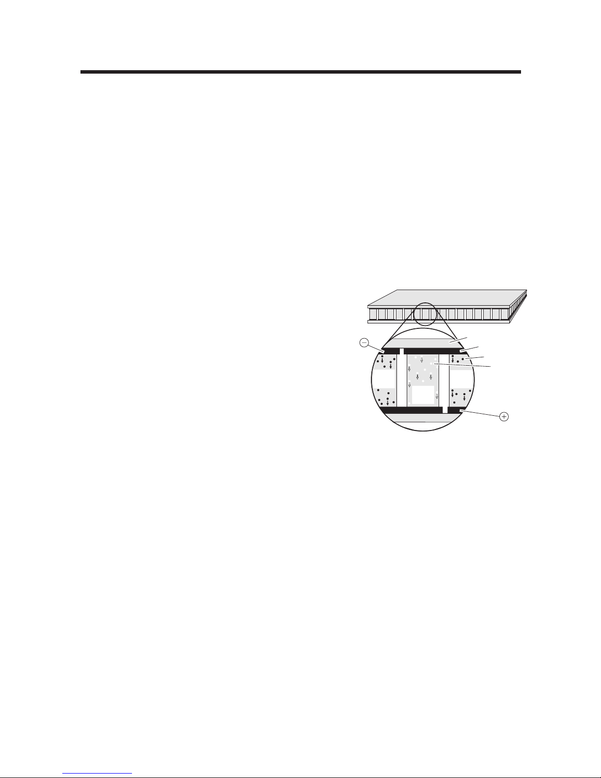
Tech Support: (888) 652-9253 • Sales: (888) 735-8437 • tech@mjr.com • www.mjr.com A-1
The functional heart of every DNA Engine® thermal cycler is a high-performance Peltier-effect heat
pump (also known as a “thermoelectric module”). The “MJ” module version is a solid-state device
manufactured to withstand the thermal stresses associated with rapidly cycling temperatures.
A thermoelectric module consists of numerous pairs of
crystalline semiconductor blocks precisely sandwiched
between two layers of ceramic substrate (fig. A-1). The
blocks are of two varieties: “N-type,” which has a surplus of electrons in its crystalline structure, and “P-type,”
which has a deficit of electrons. The two types are positioned in alternating pairs within the innermost layer of
the sandwich.
The two types of blocks are wired together in alternating pairs. When electrical current is passed through the
blocks, electrons in the N-type blocks and the “holes,”
or empty electron spaces, in the P-type blocks are excited
at one conductor-semiconductor interface, which absorbs
a small amount of heat. The electrons and holes flow
through the crystalline blocks and return to a low-energy
state at the other conductor-semiconductor interface, with the release of the previously absorbed
heat. A thermal gradient of up to 70°C can be generated across the blocks in this manner.
The direction of heat pumping is reversed by reversing the polarity of current flow through the
thermoelectric module, and the amount of heat pumped is changed by changing the amount of
current passed. Both direction and amount of current flow are dictated by a microprocessor, allowing precise control of thermal cycling in the Alpha
™
unit block.
How a Peltier Heat Pump Works
Appendix A
Electron
Hole
N-type
bismuth
telluride
N-type
bismuth
telluride
Metal conductor
P-type
bismuth
telluride
Ceramic substrate
Power input
Power input
Figure A-1 A thermoelectric module.
Page 100

 Loading...