

Page 1

MITECH ULTRASONIC
FLAW DETECTOR
MFD500B
User’s Manual
MITECH CO.,LTD.
www.mitech-ndt.com
Page 2

mvip@mitech-ndt.com
1
CONTENTS
1 Introduction...........................................................................................................................................................3
1.1 Features of the Instrument...........................................................................................................................3
1.2 Specifications................................................................................................................................................. 4
1.3 Instrument Standard Configuration............................................................................................................ 5
2 Understanding the Keypad, Menu System and Display...........................................................................5
2.1 Structure Feature...........................................................................................................................................5
2.2 Screen Display...............................................................................................................................................6
2.3 Keys and Rotary Knob Features.................................................................................................................8
2.4 Menus and Functions....................................................................................................................................9
2.5 Alarm Lights.................................................................................................................................................... 9
3 Initial Start-up.......................................................................................................................................................9
3.1 Power Supply................................................................................................................................................. 9
3.2 Connecting a Probe.................................................................................................................................... 10
3.3 Starting the Instrument............................................................................................................................... 10
4.0 Operation......................................................................................................................................................... 10
4.1 Adjusting the Display Range..................................................................................................................... 10
4.2 Setting the Material Velocity...................................................................................................................... 10
4.3 Setting the Display Delay...........................................................................................................................10
4.4 Selecting the Probe Test Mode................................................................................................................. 11
4.5 Selecting a Rectification Mode..................................................................................................................11
4.6 Setting the A-Scan Reject Level............................................................................................................... 11
4.7 Setting the Gain...........................................................................................................................................12
4.8 Changing the Gain-Adjustment Increment (DB STEP).........................................................................13
4.9 Auto Gain Feature.......................................................................................................................................13
4.10 Configuring the Gates.............................................................................................................................. 13
4.11 Setting the Damping Level.......................................................................................................................14
4.12 Setting the Pulse Energy Level.............................................................................................................. 14
4.13 Setting the Pulse Width............................................................................................................................17
4.14 Adjusting the Pulse Repetition Frequency (PRF)................................................................................17
4.15 Specifying the Probe Frequency............................................................................................................ 17
4.16 Specifying the Piezo Crystal Size.......................................................................................................... 17
4.17 Setting the Probe X-Value....................................................................................................................... 17
4.18 Probe Delay Calibration...........................................................................................................................17
4.19 Setting the Angle of Incidence................................................................................................................ 17
4.20 Magnifying the Contents of a Gate........................................................................................................ 18
4.21 Freezing the A-Scan Display...................................................................................................................18
4.22 Setting the Display Grid........................................................................................................................... 18
4.23 Selecting Units...........................................................................................................................................18
Page 3

mvip@mitech-ndt.com
2
4.24 Scale Setting..............................................................................................................................................18
4.25 Fill function................................................................................................................................................. 19
4.26 Setting the Display Brightness................................................................................................................19
4.27 Setting the Display Color......................................................................................................................... 19
4.28 Setting the A-Scan Color......................................................................................................................... 19
4.29 Setting the Menu Color............................................................................................................................ 20
4.30 Key Sound..................................................................................................................................................20
4.31 Date and Time Setting..............................................................................................................................20
4.32 Display the System Information..............................................................................................................21
4.33 Resetting the Instrument..........................................................................................................................21
4.34 Connecting to a Computer.......................................................................................................................21
5 Calibration and Measurement....................................................................................................................... 21
5.1 Calibration with Straight-and Angle-Beam Probes................................................................................ 21
5.2 Calibration with Dual-Element (TR) Probes............................................................................................23
5.3 Distance Amplitude Curve......................................................................................................................... 23
5.4 Measuring with DGS/AVG..........................................................................................................................26
5.5 Curved Surface Correction........................................................................................................................28
5.6 AWS D1.1 Weld Rating Feature............................................................................................................... 28
5.7 Crack Height Measuring Feature..............................................................................................................28
5.8 Envelope Function...................................................................................................................................... 29
5.9 Peak Hold Feature...................................................................................................................................... 29
5.10 B-Scan Feature......................................................................................................................................... 30
5.11 Weld Figure Feature................................................................................................................................. 30
5.12 Coded Echo color......................................................................................................................................30
5.13 Data Storage..............................................................................................................................................32
6 Maintenance and Care..................................................................................................................................... 33
6.1 Care of the Instrument................................................................................................................................33
6.2 Care of the Batteries................................................................................................................................... 34
6.3 Maintenance.................................................................................................................................................34
6.4 Warranty........................................................................................................................................................34
6.5 Tips on Safety.............................................................................................................................................. 34
Appendix.................................................................................................................................................................35
Appendix A: Charging the Batteries................................................................................................................35
Appendix B: Menu Structure............................................................................................................................36
User's Note: ..........................................................................................................................................................36
Page 4

mvip@mitech-ndt.com
3
1 Introduction
The MFD500B is an advanced digital ultrasonic flaw detector featuring full digital TFT LCD and a host of
new features to meet challenging inspection requirements. Combined with powerful flaw detection and
measurement capabilities, extensive data storage, it is capable for transfer detailed inspection data to
the PC via its high-speed USB port.
The instrument incorporates many advanced signal processing features including a 10MHz RF
bandwidth to permit testing of thin materials, narrow band filters to improve signal to noise in high gain
applications, a spike pulse for applications required higher frequencies and a adjustable square wave
pulse to optimize penetration on thick or highly attenuating materials.
The instrument can be widely used in locating and sizing hidden cracks, voids, disbands and similar
discontinuities in welds, forgings, billets, axles, shafts, tanks, pressure vessels, turbines and structural
components.
1.1 Features of the Instrument
The instrument extends the performance and range of applications that are capable of being satisfied by
a portable instrument. The quality, portability, durability, and dependability that you have come to expect
from the popular Mitech MFD Series instruments remain.
1 Leading Technology including full English menu, master-slave, shortcut key and rotary key
design, it is easy for operation.
2 Adopted with full digital TFT LCD, clear screen brightness, capable for choosing the
background color, waveform color and menu color. Adjustable brightness freely, suitable for operating
under different environments.
3 High performance security battery module is easy to assemble and disassemble, the instrument
can work continuously more than eight hours.
Display
Hi-resolution (320×240 pixels) full digital TFT LCD with adjustable brightness, it is capable of providing
high contrast viewing of the waveform from bright, direct sunlight to complete darkness.
The hi-resolution TFT LCD display with fast 60 Hz update gives an “analog look” to the waveform
providing detailed information that is critical in many applications including nuclear power plant
inspections.
Range
Up to 6000 mm in steel; range selectable in fixed steps or continuously variable, suitable for use on large
work pieces and in high-resolution measurements.
Pulse
Pulse Energy selectable among Low (300V), Medium (500V) and High (700V)
Pulse Repetition Frequency adjustable from 10 Hz to 1 KHz in 1 Hz increments
Damping selectable among 100Ω, 200Ω and 400Ω for optimum probe performance
Test Modes including Straight, Angle, Dual and Thru-transmission
Receiver
Sampling:10 digits AD Converter at the sampling speed of 160 MHz
Rectification:Positive Halfwave, Negative Halfwave, Fullwave and RF
Analog Bandwidth: 0.5MHz to 15MHz capability with selectable frequency ranges (automatically set by
the instrument) to match probe for optimum performance.
Gain:0 dB to 110 dB adjustable in selectable steps 0.1 dB, 2 dB, 6 dB, and locked
Gates
Two fully independent gates offer a range of measurement options for signal height or distance using
peak triggering.
The echo-to-echo mode allows accurate gate positioning for signals which are extremely close together.
Gate Start: Variable over entire displayed range
Gate Width: Variable from Gate Start to end of displayed range
Gate Height: Variable from 0 to 99% Full Screen Height
Alarms: Threshold positive/negative
Page 5

mvip@mitech-ndt.com
4
Memory
Memory of 100 channel files to store calibration set-ups
Memory of 1000 wave files to store A-Scan patterns and instrument settings.
All the files can be stored, recalled and cleared.
Video Recorder
Screen scenes can be captured as movie files. About 2 minutes movie can be saved to the inside
memory. They can be re-played using the instrument or the PC software delivered with the instrument.
Video Recorder is useful in many situations, convenient for those who want to analyze the probing
activities later.
Functions
Semiautomatic two point calibration: Automated calibration of transducer zero offset and/or material
velocity
Flaw Locating:Live display Sound-path, Projection (surface distance), Depth, Amplitude,
Flaw sizing: Automatic flaw sizing using AVG/AVG or DAC, speeds reporting of defect acceptance
or rejection.
Digital Readout and Trig. Function: Thickness/Depth can be displayed in digital readout when using
a normal probe. Sound-path, Surface Distance and Depth are directly displayed when using angle
probe.
Both the DAC and the AVG method of amplitude evaluation are available.
Curved Surface Correction Feature
Crack Height Measure Function
Weld Figure Feature
Magnify Gate:spreading of the gate range over the entire screen width
Video Recording and Play
Auto-gain Function
Envelope: Simultaneous display of live A-scan at 60 Hz update rate and envelope of A-scan display
Peak Hold: Compare frozen peak waveform to live A-Scans to easily interpret test results.
A Scan Freeze:Display freeze holds waveform and sound path data
B Scan display feature
AWS D1.1 Feature
Real Time Clock
The instrument clock keeps running tracking the time.
Communication
High Speed USB2.0 Port
The DataPro software helps manage and format stored inspection data for high-speed transfer to the PC.
Data can be printed or easily copied and pasted into word processing files and spreadsheets for further
reporting needs. New features include live screen capture mode and database tracking.
Battery
Internal rechargeable Li-ion battery pack rated 7.2V at 8800 mAh
8 hours nominal operating time depending on display brightness
8-10 hours typical recharge time
Knob
Operating adjustments are easily and quickly made using the rotary knob.
1.2 Specifications
Range: 0 to 9999mm, at steel velocity
Material Velocity: 300 to 15000m/s
Display Delay: -20 to 3400 µs
Probe Delay/Zero Offset : 0 to 99.99µs
Sensitivity Leavings:>60dB (flat-bottomed deep hole 200mmФ2)
resolution :>40dB (5P14)
Noise Level: ≤ 8%
Test Modes: straight ,angle, dual element and thru-transmission
Page 6

mvip@mitech-ndt.com
5
Pulse Repetition Frequency ranges from 10 Hz to 1000 Hz
Pulse Energy: Low (300V), Medium (500V) and High (700V) spike pulse.
Damping: 100Ω, 200Ω and 400Ω
Bandwidth (amplifier bandpass ): 0.5 to 15MHz
Gate Monitors: Two independent gates controllable over entire sweep range
Rectification: Positive half wave, negative half wave, full wave, RF
System Linear Error: Horizontal: +/-0.1% FSW, Vertical: 0.25% FSH, Amplifier Accuracy +/-1 dB.
Reject (suppression): 0 to 80% full screen height
Units: Inch or millimeter
Transducer Connections: BNC or LEMO
Power Requirements: AC Mains 100-240 VAC, 50-60 Hz
Overall Dimensions:263H×170W×61D mm
Relative Humidity:(20 ~ 95)% RH
Power Supply:DC 9V
Operating Temperature: -10℃ to 50℃
Storage Temperature: -30℃ to 50℃
1.3 Instrument Standard Configuration
No.
Item
Qty
Remarks
Standard
config.
1
Main unit
1
with full digital TFT LCD Display
2
Straight Beam Probe
1
4 MHz, Φ10
3
Angle Beam Probe
1
4 MHz, 8 mm×9 mm, 60°
4
Probe Cable
1
Q9-C5,or optional C9- C5
5
Battery Module
1
8.8 amp hour (MB-02)
6
Power Adapter
17Supporting pillar
1
8
Attached files
1
9
Datapro Software
1
10
USB Cable
1
11
Power Cable
1
12
ABS Case
1
Optional
config.
1
Protective Cover for Main Unit
2
Dual-crystal Straight Probe
2 Understanding the Keypad, Menu System and Display
2.1 Structure Feature
The right figure gives an overview
of the instrument system.
1、The Main Unit
2、Probe (Transducer)
Page 7
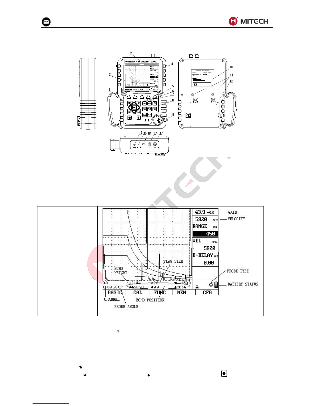
mvip@mitech-ndt.com
6
The Main Unit
1.Belt 2.LCD Display 3.LOGO 4. Hooks 5. Menu Keys
6. Alarm LED 7. Power LED 8. Keypad 9. Rotary Knob
10. Product Label 11.Support Pillar Screw 12. Battery Case
13. Power adapter port 14. Battery Switch 15. USB Socket
16., Probe Cable Port (Transmit) 17. Probe Cable Port (Receive)
2.2 Screen Display
The instrument displays are designed to be easy to interpret.
The Instrument has a
digital screen for the
display of A-Scan.
The status line below
the wave display shows
values of range settings
and measured values.
On the first status line
Echo height is displayed as: 24.5%. It means that the peak echo height inside the current selected
gate is 24.5% FSH (Full Screen Height of the wave area).
Flaw size value means ERS (Equivalent Reflector Size) of the reflector signal inside the current
selected gate. It is displayed after the AVG curve is switched on. When the DAC curve is on, this
value will be displayed as the dB offset of the peak echo inside the current selected gate to the
reference DAC curve (DAC→OFFSET→SIZE REF).
The icon ‘ ’ indicates that the horizontal scale is displayed as sound path (S-PATH). It can be
changed to ‘ ’ (Projection value) or ‘ ’ (Depth) by simply pressing repeatedly.
Page 8
mvip@mitech-ndt.com
7
On the second status line, it shows the channel file name, the beam angle and the measured value of
the peak echo ( : Sound path. : Projection. :Depth) inside the current selected gate.
“A 61.3” means gate mode is single; current selected gate is gate A; and peak echo position: sound
path 61.3 mm.
“AB 24.0” means Echo-Echo mode of the gates; selected gate is gate A; sound path: 24.0 mm.
The names of the menus or submenus
are displayed at the bottom of the screen.
The selected menu or submenu is
highlighted.
Indicated at the right of the display, next
to the A-Scan, are the functions of the
corresponding menu.
The status area at the bottom-right corner
shows the system status. The following
status will be showed:
: Indicates the battery capacity
: Straight beam probe
: Angle beam probe
: Dual element probe
: Through-transmit mode
: Envelope function on
: Peak hold function on
: USB online; : A-Scan freezed
Page 9

mvip@mitech-ndt.com
8
The status area at the top-right corner
indicated shows the system gain and the
sound velocity.
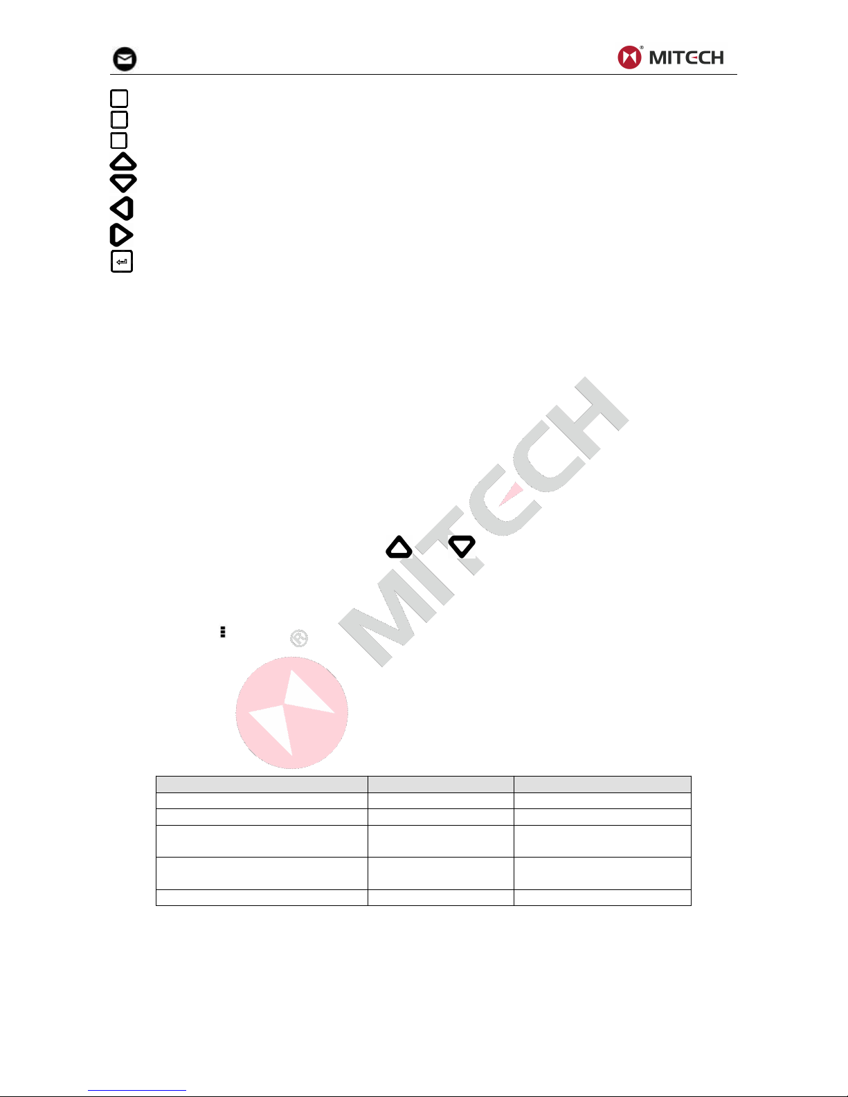
2.3 Keys and Rotary Knob Features
To access any function:
Press one of the five menu keys (F1~F5) to select a menu. The menus across the
bottom of the display will immediately be replaced with the submenus contained in the
selected menu
Press a menu key (F1~F5) again to select the submenu containing the desired function.
Press and to move the cursor to select the desired function.
Change the value listed in the function box with the rotary knob. Some values can also
be adjusted with repeatedly pressing the knob.
Special keys such as Gain, Gate, Range, Probe Zero-Offset Calibration, Angle Calibration,
Freeze, Save Waveform, Auto-Gain, Envelop, Peak Hold and etc. are grouped together for
easy thumb control. This design allows direct access to important instrument set-up
parameters and provides easy and fast operating in difficult inspection environments
Functions of the keys:
Home key immediately returns the instrument to the main screen (full screen)
Freeze key freezes the A-Scan
Magnify key expands the gate range to full screen
For turning the instrument On/Off
Db-Step key selects the gain submenus or switch the db step
A
/
B
Gate key - Gate functions selecting gate functions and Gate A/B switch
Range key - Range function selecting
Probe-Delay key – Probe Delay calibration
Probe-Angle key selects the angle calibration functions
Save key performs a data-storage of the A-Scan pattern
G
A
I
N
A
U
T
O
Auto-Gain key starts or stops the Auto-Gain function
L
O
P
E
E
N
V
E
Envelope key turns the Envelope function on and off
The instrument is designed to
give the user quick access to all
of the instrument’s functions.
Its easy-to-use menu system
allows any function to be
accessed with no more than
three key presses.
The instrument is designed to
give the user quick access to all
of the instrument’s functions.
Its easy-to-use menu system
allows any function to be
accessed with no more than
three key presses.
Page 10
mvip@mitech-ndt.com
9
P
E
A
K
H
O
L
D
Peak-Hold key turns the Peak-Hold function on and off.
V
I
D
E
O
Video key starts or stops recording a segment of the display
D
A
C
A
V
G
DAC-AVG key selects the menus of DAC/AVG
Up Arrow key – Move the cursor up to select the desired function
Down Arrow key – Move the cursor down to the desired function
searches next echo towards left, or move the cursor to left when inputting digit numbers.
searches next echo towards right, or move the cursor to right when inputting digit numbers.
confirms or switches current selection
Rotary knob makes it convenient for handling device parameters and functions. It supports three
operations: turn clockwise, turn counter-clockwise and single press.
Turn clockwise: increase the selected parameter, or change the selection.
Turn counter-clockwise: decrease the selected parameter, or change the item selection.
Single press: changes mode between coarse and fine parameter adjustments or changes item selection.
2.4 Menus and Functions
The instrument menu system consists of several menus, submenus, and functions. It allows the operator
to select and adjust various features and instrument settings.
Available menus are accessed via the Home Menu. Note that the menus visible on your particular
instrument depend on which options are installed.
Each menu contains several submenus.
Menus and submenus are selected by pressing the key below the desired item (F1 to F5).
When a submenu is selected, the functions contained in that submenu are listed in the Function Bar
down the right-hand side of the display screen.
Functions are then selected by pressing and .
Turning the Function Knob will change the value shown in the selected function’s box.
Note that some functions, like RANGE, have both coarse and fine adjustment modes. There are three
steps in the fine adjustment mode. Coarse and fine modes are selected by pressing the knob more than
once. An icon of “ ” will appear on the left of the function name when the function is in fine adjustment
mode. When the function is in coarse adjustment mode, turning the function knob will produce large
changes in the selected function’s value. When the function is in fine adjustment mode, rotating the
function knob will change the value by smaller amounts.
2.5 Alarm Lights
Two alarm lights appear at the top-right corner front of the instrument’s keypad. One alarm light is
marked as ALRM, which is assigned to the gate alarm. When a gate alarm is triggered, this light will
illuminate. The other light is marked as PWR indicating power and battery status.
Status
ALRM LED
PWR LED
Gate alarm
Red on
×
Battery charging
×
Flash red/green
Battery charge completed with
external power connected
×
Green on
External power connected
No battery installed
×
Green on
No external power
×
off
3 Initial Start-up
3.1 Power Supply
The instrument can be operated with an external power adapter or with batteries.
You can connect the instrument to the mains supply system even if it carries batteries. A discharged
battery is charged in this case, viz. parallel to the instrument operation.
Operation Using the Power Supply Unit
Page 11
mvip@mitech-ndt.com
10
Connect the instrument to the mains socket-outlet using the power supply unit. The plug receptacle is at
the top left of the instrument. Push the plug of the power supply unit into the plug receptacle until it snaps
into place with a clearly audible click. The PWR LED on the keypad of the instrument will light in green
color if the connection is properly aligned
Operation Using Batteries
Use a lithium-ion battery pack provided with the instrument for the battery operation.
The battery compartment is situated at the instrument back. The cover is fastened with 4 screws To
insert the battery pack
Loosen the four screws of the battery cover.
Lift the cover off upward.
Insert the battery into the battery compartment.
Close the battery compartment and fasten the screws.
Turn on the instrument to make sure the battery is installed correctly and firmly.
Note:
The battery switch on the top of the instrument must be set to ON when operating with the battery
pack or charging it.
When not using the instrument, set the switch to OFF to save power.
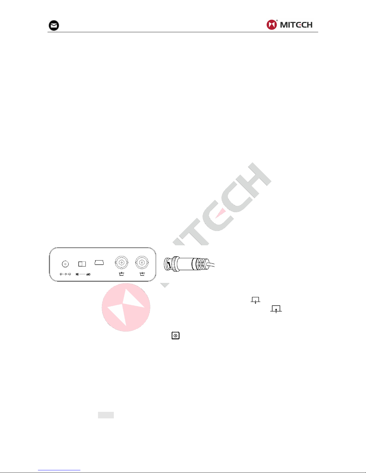
3.2 Connecting a Probe
To prepare the instrument for operation, you have to connect a probe to it. The instrument is available
with the probe connectors BNC (LEMO connectors are optional).
When connecting a probe to the instrument, it’s not only important that the probe’s physical connection
be properly made. It’s also important that the instrument is properly configured to work with the installed
probe. The Instrument will operate with one or two single-element probes or with a dual-element probe.
To install a single-element probe, connect the probe cable to either of the two ports on the front of the
instrument. When two probes or a dual-element probe is connected to the instrument, the “Receive”
probe connector should be installed in the right port and the ‘Transmit’ probe connector in the left port.
3.3 Starting the Instrument
To start the instrument, press the switch-on key . If it operates on the internal battery pack, make sure
to set the battery switch to ON position before starting.
The start display of the instrument appears; here you will also see the current software version and the
serial number of the instrument. The instrument carries out a self-check and then switches over to
stand-by mode.
The settings of all function values are the same as before switching-off of the instrument.
The instrument will shut off automatically when the battery capacity level is too low.
4 Operation
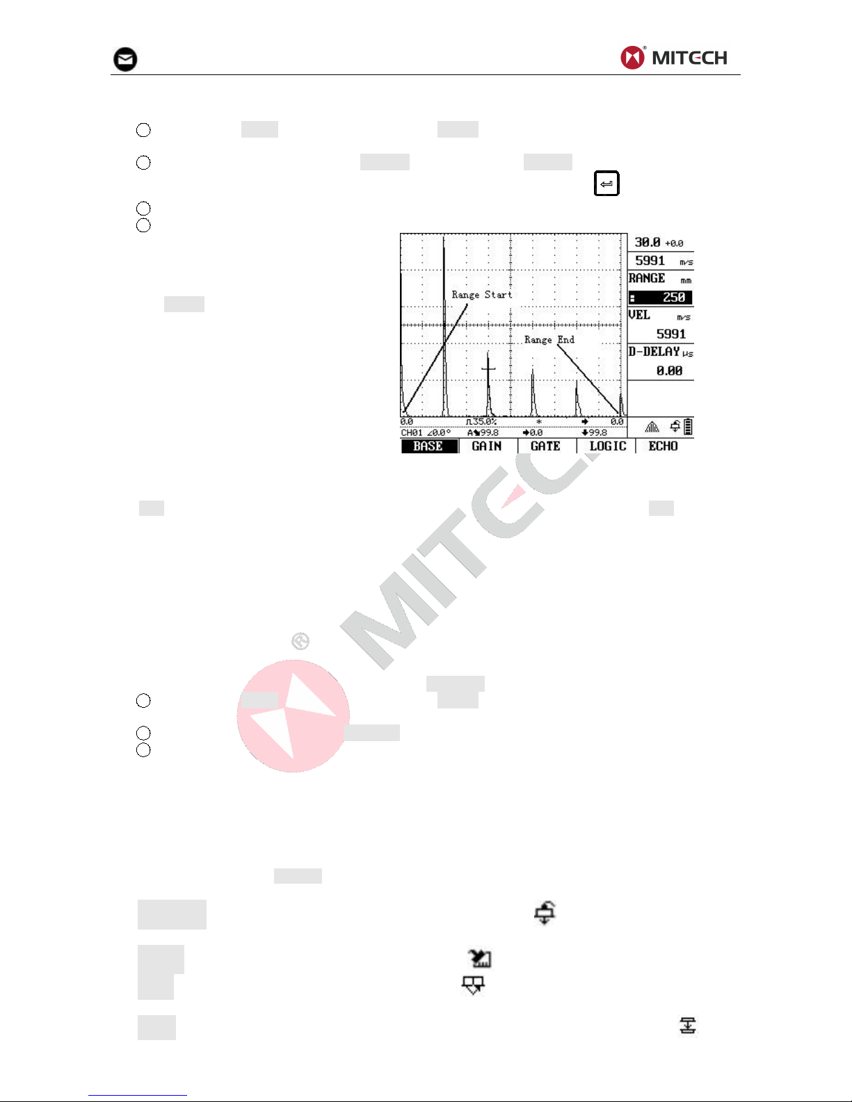
4.1 Adjusting the Display Range
The function group BASE enables you to make the basic adjustment of the display range. The display on
the screen must be adjusted for the material to be tested and for the probe used.
Calibration requires the use of calibrated standard made of the same material as the test piece. Prior to
calibrating the instrument/probe combination, the A-Scan display-screen range (the material thickness
Connect one single element
probe to either port.
Connect leads from a Dual
Element Probe to both ports.
For through-transmission,
connect two single element
probes to the transmit (left,
labeled as ) and receive
(right, labeled as ) ports.
Page 12
mvip@mitech-ndt.com
11
value represented by the full horizontal width of the screen) will normally be set to a value equal to or
slightly larger than the calibrated standard.
1 Activate the BASE submenu (located in the BASIC menu) by pressing the menu key below it.
Three functions will appear down the right side of the display screen.
2 Select the function item titled RANGE. You’ll note that RANGE has both coarse and fine
adjustment modes. Coarse and fine modes are selected by repeatedly pressing .
3 To change the range, turn the knob.
4 The display’s horizontal range will remain as set.
Range is adjustable in fixed steps or
continuously variable.
4.2 Setting the Material Velocity
Use VEL to set the sound velocity within the test object. Always ensure that the function VEL is correctly
set. The instrument calculates all range and distance indications on the basis of the value adjusted here.
Velocity range:300m/s~15000m/s
Coarse adjustment, in steps as follow
2260m/s 2730m/s 3080m/s 3230m/s
4700m/s 5920m/s 6300m/s
4.3 Setting the Display Delay
Here you can choose whether to display the adjusted range (for example 300 mm) starting from the
surface of the test object, or in a section of the test object starting at a later point. This allows you to shift
the complete screen display and consequently also the display zero. If the display should for example
start from the surface of the test object, the value in D-DELAY must be set to 0. To set the display delay
1 Activate the BASE submenu (located in the BASIC menu) by pressing the menu key below it.
Three functions will appear down the right side of the display screen.
2 Select the function item titled D-DELAY.
3 To change the display delay, turn the knob. You’ll note that the displayed echoes shift to the left
or right.
D-DELAY range: -20~3400 µs
Coarse adjustment: 12 pixel space (in µs)
Fine adjustment: 1 pixel space (in µs)
4.4 Selecting the Probe Test Mode
You can use the function PROBE to activate the pulse-receiver separation. The following modes are
available:
STRAIGHT- For single straight beam transducer operation ( will be displayed).The probe
connection sockets are connected in parallel.
ANGLE- For single angle beam transducer operation ( will be displayed)
DUAL – For the use with dual-element (TR) probes ( will be displayed); the right-hand socket is
connected with the amplifier input whereas the initial pulse is available at the left-hand socket.
THRU – Through-transmission mode for the use with two single-element probes ( will be
Page 13

mvip@mitech-ndt.com
12
displayed); the receiver is connected with right, the pulse is connected with left.
Select the probe model step:
1 Activate the PROBE submenu (located in the CAL menu) by pressing the menu key below it.
2 Select the function item titled PROBE.
3 To change the probe mode, turn the knob. Each available probe mode is represented by an icon
on screen display whenever that probe mode is indicated.
4 The probe mode will be set to the last one displayed.
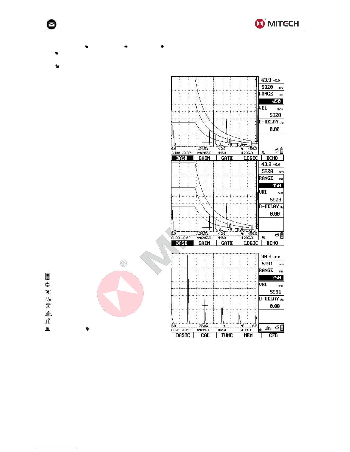
4.5 Selecting a Rectification Mode
You can select the rectification mode of the echo pulses according to your application in the function
RECTIFY (BASIC→ECHO→RECTIFY).
Rectification affects the orientation of the A-Scan on the display screen. The A-Scan represents the
pulse (echo) that’s returned from the material being tested to the instrument. The series of echoes looks
like the Radio Frequency (RF) signal.
Note that the RF signal has a negative
component below the axis, and a positive
component above the axis.
RF rectification is useful when evaluating a
probe.
RF rectification is forbidden when displaying
the DAC/AVG curves.
Positive Half Rectification means that only
the upper (positive) half of the RF signal is
displayed.
Negative Half Rectification means that only
the bottom (negative) half of the RF signal is
displayed. In the figure above, note that
even though it’s the negative half of the RF
signal, it’s displayed in the same orientation
as a positive component. This is only to
simplify viewing. The signal displayed in the
view identified as Negative Rectification is
the negative component of the RF signal.
Full-Wave Rectification combines the
positive and negative rectified signals
together, and displays both of them in a
positive orientation. Full-wave rectification is
recommended for most inspections.
Use the following procedure to select a rectification mode
1 Activate the ECHO submenu (located in the BASIC menu) by pressing the menu key below it.
Page 14

mvip@mitech-ndt.com
13
Three functions will appear down the right side of the display screen.
2 Select the function item titled RECTIFY. You’ll note that there are four options:
POS- Shows the positive component of the RF signal
NEG- Shows the negative component of the RF signal but displays it in a positive orientation
FULL-Shows the positive and negative halves of the RF wave, but both are oriented in the positive
direction.
RF- Shows the echo with no rectification
3 Select the rectification method.
4.6 Setting the A-Scan Reject Level
The function REJECT allows you to suppress unwanted echo indications, for example structural noise
from your test object. To omit a portion of the A-Scan, you must define the percentage of full-screen
height you wish to omit. You may omit A-Scan up to 80% of the screen height. To set a reject percentage
1 Activate the ECHO submenu (located in the BASIC Menu) by pressing the menu key below it.
2 Select the function item titled REJECT.
3 Set the required percentage value by turning the knob.
You should handle this function with great caution, as it may of course happen that you suppress echoes
from flaws as well. Many test specifications expressly forbid using the reject function.
4.7 Setting the Gain
Instrument gain, which increases and decreases the height of a displayed A-Scan, is adjusted with the
gain functions.
The gain includes the basic gain, the
offset gain and the correction gain. The
basic gain and the correction gain are
also displayed on the top-right corner of
the screen.
The maximum of the total gain (the basic
gain plus the offset gain plus the
correction gain) is 110 dB.
The offset gain is for the purpose of flaw evaluation. The DAC/AVG curves remain unchanged when
adjusting the offset gain.
Sensitivity correction gain: Compensate for the transfer losses in the material under test. This correction
gain is necessary if test object and reference block have different surface qualities. You have to find out
the adjustment value for the compensation of transfer losses by experiments. The gain is varied
accordingly in this correction, while the curve line remains unchanged. To set the sensitivity correction
gain, select the function T-CORR and then adjust its value according to the experiment.
When DAC is active, adjusting the basic gain setting will result in an equal adjustment of the DAC curve
position. To increase the instrument gain without changing the DAC curve position, please use the
T-CORR function to compensate for varying coupling/surface conditions.
4.8 Changing the Gain-Adjustment Increment (DB STEP)
When adjusting the A-Scan Gain, each click of the adjustment knob increases or decreases the gain
level by a dB increment equal to the DB STEP. Several values can be specified for DB STEP. Available
increments include: 0.1dB, 1dB, 2dB, 6dB and 0dB. Note that setting the DB STEP to 0dB prevents
adjustment of the instrument gain and prevents any changes using the knob.
To select one of the existing DB STEP values:
1 Activate the GAIN submenu (located in the BASIC menu) by pressing the menu key below it.
2 Select the function item titled DB STEP.
Page 15

mvip@mitech-ndt.com
14
3 Change the DB STEP value by repeatedly pressing key or by turning the knob.
Note that DB STEP value can be quickly changed by repeatedly pressing the key .
4.9 Auto Gain Feature
Use the Auto Gain function to automatically set the basic gain, so as to adjust the peak echo inside the
currently selected gate to a target height.
1 Set the target echo height using the AUTO function located in the FUNC submenu.
2 Press
GAIN
AUTO
to start the Auto Gain function. “AUTO-XX%” will be shown on the screen.
3 The Auto Gain function will end when the echo height reaches the target value. Or you can stop
the function by pressing
G
A
I
N
A
U
T
O
again.
4.10 Configuring the Gates
The gates monitor the range of the test object where you expect to detect a flaw. If an echo exceeds or
falls below the gate, an alarm signal is shown via the ALRM LED. The gate chooses the echo for the
digital time-of-flight or amplitude measurement.
The instrument has two gates: gate A and B. Gate A and B are independent of one another. Setting the
position and characteristics of the A- and B-Gates is the first step to configuring the instrument for flaw
detecting or material-thickness measurement. The GATE functions controls not only the location of the A
and B-Gates, but also the alarms and other features activated when an A-Scan signal crosses a specific
gate.
A-Scan signals crossing the A or B-Gate are evaluated for the purposes of flaw detection and
material-thickness evaluation. When the signal crosses the A or B-Gate, the maximum point (peak) of
the signal (in the specific gate) is used for evaluation purposes. The measured value is indicated on the
status line.
Selecting a Gate
Selecting a gate by using the GATE SEL
function in the GATE submenu.
You can also repeatedly press
A
/
B
to
switch the selected gate between Gate A
and Gate B.
The selected gate will be shown in solid
line. The unselected gate will be shown in
dashed line.
Positioning Gates
Use the following procedures to set the vertical and horizontal position of the A and B-Gates. Remember
that gate position has the following effects on instrument performance:
A-Scan echoes on the right side of the display screen represent features that occur at a greater
depth from the test-material surface than those on the left of the display screen. Therefore, moving a
gate to the right means that the gate is evaluating a deeper portion of the test material.
A wider gate will simply span the equivalent of more test-material depth
Increasing the vertical height (called threshold) of a gate means that only reflected signals of
sufficiently large amplitude will cross the gate.
Setting a Gate’s Starting Point
You can fix the starting point of the gates A or B within the display range.
1 Activate the GATE submenu (located in the BASIC menu).
2 Select the gate to be positioned using the GATE SEL function.
3 Select the gate START function and adjust the starting point by turning the knob. Increasing and
decreasing the value of the starting point moves the gate to the right and left, respectively.
Page 16

mvip@mitech-ndt.com
15
4 The gate starting point will remain as set, even when width adjustment is made.
Coarse adjustment: half of a lattice
Fine adjustment: 1 pixel space
When the gate exceeds the display range,
as shown in right figure, the measured
value will be shown as “*” on the status
line.
You can also set the selected gate’s starting point using the Quick Search Function. Quick Search
Function is achieved by simply pressing the and . Note that the instrument will only search the
echo whose peak crosses the selected gate in this function.
Adjusting a Gate’s Width
You can determine the threshold value of the gates within the range of 0 to 99% FSH (Full Screen Height)
for triggering the LED alarm if this value is exceeded or not reached, depending on the setting of the
LOGIC function.
1 Activate the GATE submenu (located in the BASIC menu).
2 Select the gate to be positioned using the GATE SEL function.
3 Select the gate WIDTH function and adjust its value by turning the knob.
Setting a Gate’s Threshold (Vertical Position)
You can determine the threshold value of the gates within the range of 0 to 99% FSH (Full Screen Height)
for triggering the LED alarm if this value is exceeded or not reached, depending on the setting of the
LOGIC function.
1 Activate the GATE submenu (located in the BASIC menu).
2 Select the gate to be positioned using the GATE SEL function.
3 Select the THRESH function and adjust the vertical height by turning the knob. Increasing and
decreasing the value of the threshold moves the gate up and down, respectively.
Defining B-Gate Alarm Logic
This function allows you to choose the method for triggering the B-Gate alarm.
Gate alarms can be set to trigger when an A-Scan echo crosses the gate (POSITIVE logic) or when no
echo crosses the gate (NEGATIVE logic) within the displayed range.
A-Gate is locked to POSITIVE logic. And
B-Gate can be set to either POSITIVE or
NEGATIVE.
The appearance is different between the
POSITIVE gate and the NEGATIVE gate when
displayed, as is shown in right figures.
Note that the alarm and measurement function
of the gates is only active within the display
range.
Use the following procedure to specify B-Gate
logic:
Page 17

mvip@mitech-ndt.com
16
1 Activate the LOGIC submenu (located
in the BASIC menu) by pressing the menu key
below it.
2 Select the B-LOGIC function and
choose the gate-alarm triggering logic.
Turning the Audible Alarm On or Off
When a gate alarm is activated, one or more of the following will occur:
An alarm indication light on the front of the instrument will illuminate
An audible alarm (HORN) will sound
Use the following procedure to turn the horn off or on:
1 Activate the LOGIC submenu (located in the BASIC menu) by pressing the menu key below it.
2 Select the ALARM function and turn the audible alarm ON or OFF.
Setting the Gate Work Mode
Two options for the gate work mode: SINGLE and E-E.
SINGLE: measures the distance from the work piece surface to the peak echo inside the selected gate.
E-E (Echo-Echo mode): measures the distance between two peak echoes (the two peak echoes should
be selected by two gates). It is useful in thickness measuring.
Use the GATE MODE function in the LOGIC submenu to select the gate work mode.
Page 18

mvip@mitech-ndt.com
17
Gate Mode: Single
Gate Mode: E-E
4.11 Setting the Damping Level
Note: For this model, the parameter is fixed.
This function serves for matching the probe. You can use it to adjust the damping of the probe’s
oscillating circuit and to consequently change the height, width and resolution of the echo display.
1 Activate the PULSER submenu (located in the CAL menu) by pressing the menu key below it.
2 Move the cursor to the selection titled DAMPING.
3 To change the specified damping level and optimize the A-Scan signal appearance, turn the
knob. You’ll note that the following damping levels are available: 100Ω、 200Ω、400Ω.
4 The damping level will be set to the one last displayed.
4.12 Setting the Pulse Energy Level
Use the function ENERGY to set the pulse voltage. The relative energy with which the pulse fires can be
selectable set to LOW, MEDIUM or HIGH.
The setting MEDIUM is recommended for most inspections. HIGH is used for inspections in which
maximum sensitivity is import, e.g. for the detection of small flaws. Choose the setting LOW for
broadband probes or if narrow echoes are required (better lateral resolution).
To set the pulse energy
1 Activate the PULSER submenu (located in the CAL menu) by pressing the menu key below it.
2 Select the function item titled ENERGY.
3 Select the energy level by turning the knob or continuing to press the key.
4.13 Setting the Pulse Width
The function is no available in this model.
4.14 Adjusting the Pulse Repetition Frequency (PRF)
The pulse repetition frequency indicates the number of times an initial pulse is triggered per second. You
can determine whether you need the highest possible PRF value, or whether you are satisfied with a low
value.
The PRF value ranges from 10 Hz to 1000 KHz. The larger your work piece, the smaller PRF values are
needed in order to avoid phantom echoes. In the case of smaller PRF values, however, the A-Scan
update rate becomes lower, for this reason, high values are required if a work piece should be scanned
fast.
The best way to determine the suitable PRF value is by experimenting: start from the highest step and
reduce the value until there are no more phantom echoes.
To set the PRF level
1 Activate the PULSER submenu (located in the CAL menu) by pressing the menu key below it.
2 Select the function item titled PRF.
3 Change the PRF value by turning the knob.
4.15 Specifying the Probe Frequency
In this function, you can specify the probe frequency according to the frequency of your probe. The
instrument will automatically utilize a built-in filter to match the probe frequency.
1 Activate the PROBE submenu (located in the CAL menu) by pressing the menu key below it.
2 Select the function item titled FREQ.
3 To change the specified frequency, turn the knob.
4 The probe frequency will be set to the last one displayed.
4.16 Specifying the Piezo Crystal Size
Use DIAMETR function to set the Piezo Crystal Size of your probe. This value is required when
programming the AVG.
4.17 Setting the Probe X-Value
Page 19

mvip@mitech-ndt.com
18
The function X-VALUE enables you to set
the X-Value (distance between the probe’s
leading face and probe index/sound exit
point) of the probe used. This value is
required for the automatic calculation of the
reduced projection distance in angle beam
transducer operation.
Adjustment range: 0~50 mm
4.18 Probe Delay Calibration
Each probe has a delay line between the transducer element and the coupling face. This means that the
initial pulse must first pass through this delay line before the sound wave can enter the test object. You
can compensate for this influence of the delay line in the function P-DELAY.
If the value for P-DELAY is not known, read Chapter 5 in order to determine this value.
4.19 Setting the Angle of Incidence
The ANGLE function enables you to adjust the angle of incidence of your probe for the material used.
This value is required for the automatic calculation of the flaw position. The angle of incidence for the
straight-beam probe is fixed to 0°.
Adjustment range: 0°~80°.
4.20 Magnifying the Contents of a Gate
Whenever an A-Scan is active, pressing the key enlarges the displayed portion of the A-Scan
contained in the selected gate. Any of the available gates may be specified as the selected gate. The
width of the magnified gate determines the level of magnification since the display is magnified until the
gate width equals the full-screen width. The display will contain the magnified view until pressing
again.
Before Magnifying
After Magnifying
4.21 Freezing the A-Scan Display
Whenever an A-Scan is active, pressing freezes the A-Scan display. The active A-Scan will remain
as it appeared when was pressed and the display will remain frozen until is pressed again.
4.22 Setting the Display Grid
1 Activate the SYS submenu (located in the CFG menu) by pressing the menu key below it. Four
functions will appear down the right side of the display screen.
2 Select the function item titled GRID.
3 To change the grid type, Press key or turn the knob. Each grid style is shown in the
Page 20

mvip@mitech-ndt.com
19
display screen’s A-Scan window as it is selected. You’ll note that the following styles are available:
G1-Ten major horizontal and five vertical divisions, with two major horizontal and vertical divisions.
G2-Two major horizontal and vertical divisions.
G3-No on-screen grid. Only display-edge marks are visible.
G4- Ten major horizontal and five vertical divisions.
4 The grid style will be set to the last one displayed.
4.23 Selecting Units
In the function UNITS you can choose your favorite unit system between METRIC and IMPERIAL unit
systems.
1 Activate the SYS submenu (located in the CFG menu) by pressing the menu key below it.
2 Select the function item titled UNITS. You’ll note that the following options are available:
METRIC-metric unit system.
IMPERIAL-Imperial unit system
3 To change the units of measurements, Press key or by means of the knob.
4 The unit of measurement will be set to the choice last displayed.
4.24 Scale Setting
As an alternative to the measured values, the instrument enables to display a scale on the first status
line. The scale gives you an overview of the position of echoes.
The following settings are possible:
S-PATH: Display of sound path scale
P-VALUE: Display of projection distance
scale
DEPTH: Display of depth distance scale
Select the function SCALE. Then use the knob to set the required display mode.
As an alternative, you can repeatedly press to switch the scale.
4.25 Fill function
The function FILL toggles between the filled and the normal echo display mode. The filled echo display
mode improves the echo perception due to the strong contrast, especially in cases where workpieces
are scanned more quickly.
4.26 Setting the Display Brightness
Use the function BRIGHT to set the display brightness. You can choose between four brightness options:
25%, 50%, 75% and 100%.
1 Activate the LCD submenu (located in the CFG menu) by pressing the menu key below it. Four
functions will appear down the right side of the display screen.
Page 21

mvip@mitech-ndt.com
20
2 Select the function item titled BRIGHT.
3 To change the brightness level, Press key or turn the knob.
4 The display brightness will remain at the level last displayed.
Note: For the 25% option, the instrument consumes less current and consequently increases the
operating time in battery operation.
4.27 Setting the Display Color
The SYS COLOR value determines the color of the background, the gate and the DAC/AVG curves. All
color schemes are recommended for indoor operation while S0 and S3 are best suited for outdoor
operation.
1 Activate the LCD submenu (located in the CFG menu) by pressing the menu key below it. Four
functions will appear down the right side of the display screen.
2 Select the function titled SYS COLOR. There are nine preset color schemes.
3 To change the display’s color scheme, turn the knob.
4 The display color will remain at the scheme last displayed.
4.28 Setting the A-scan Color
1 Activate the LCD submenu (located in the CFG menu) by pressing the menu key below it.
2 Select the function titled WAV COLOR. There are seven A-Scan color options.
3 To change the A-Scan’s color, turn the knob.
4 The A-Scan echo will remain the color last displayed.
4.29 Setting the Menu Color
1 Activate the LCD submenu (located in the CFG menu) by pressing the menu key below it.
2 Select the function titled MNU COLOR. There are ten color options.
3 To change the menu’s color, turn the knob.
4 The menu will remain the color last displayed.
4.30 Key Sound
The key sound can be turned on/off using the KEY SOUND function located in the HORN submenu
(CFG→HORN→KEY SOUND).
4.31 Date and Time Setting
For a correct documentation you should always make sure that you are using the correct date and time
setting.
1 Activate the INFO submenu (located in the CFG menu) by pressing the menu key below it. Four
items will appear down the right side of the display screen.
2 Select the function Y-M-D. The
date is displayed in Year-Month-Day format.
Note that the first time you press the knob,
the year item is highlighted. The next time
you press the knob, the month item is
highlighted. Finally, pressing the knob will
cause the day item to be highlighted.
3 To change the year, month or days, turn the knob while the desired item is highlighted.
4 When complete, press the one more time. The current date will be set to the date
displayed.
Time is displayed in Hour-Minute format. And the time setting procedure is similar to that of the date.
Page 22

mvip@mitech-ndt.com
21
Once set, the internal clock of the instrument will maintain the current date and time.
4.32 Display the System Information
You can enter the INFO submenu to see the software version and the serial number of the instrument.
The VERSION and the S/N values are read-only. They cannot be modified by the user.
4.33 Resetting the Instrument
In case the instrument can no longer be operated, or you need to make a basic initialization (factory
setting), you can reset the instrument to original.
The instrument can be reset by the SYS RESET function. All the memory data, including the wave files,
the channel files and the video files, will be cleared during system reset. And the instrument settings will
be reset to default.
To reset the instrument
1 Activate the RESET submenu (in the MEM menu) by pressing the menu key below it.
2 Press the and key to select the SYS RESET function.
3 Press key or turn the knob to trigger the reset action. It will prompt out “Reset to
original?”. Press the menu key below YES to confirm the reset operation. Or press the menu key below
NO to cancel the reset operation.
NOTE:
The effects of resetting the instrument may not be reversed.
No key action should be performed during resetting process.
4.34 Connecting to a Computer
The instrument is equipped with a USB port at the upper left of the instrument. The PC can be connected
with the instrument via the USB port. A-Scan display, instrument settings, and videos stored in the
memory of the instrument can be transferred to the computer through the USB port. Detailed information
of the communication software and its usage refer to the DataPro software manual.
5 Calibration and Measurement
Before working with the instrument, you have to calibrate the instrument: you have to adjust the material
velocity and display range and allow for the probe delay depending on the material and dimensions of
the test object.
To ensure a safe and proper operation of the instrument, it is necessary that the operator be adequately
trained in the field of ultrasonic testing technology.
Below you will find some examples of common calibration methods for certain test tasks.
5.1 Calibration with Straight- and Angle-Beam Probes
Case A: With Known Material Velocity
Calibration process
1 Set the known material velocity in VEL function.
2 Couple the probe to the calibration block.
3 Set the required display range in RANGE. The calibration echo must be displayed on the
screen.
4 Position the gate on one of the calibration echoes until the sound path of the echo is indicated in
the measurement line.
5 After this, change the adjustment of the function P-DELAY until the correct sound path for the
selected calibration echo is indicated in the measurement line.
Example:
You are carrying out the calibration with a straight probe for the calibration range of 300 mm via the
function group BASE using the calibration block DB-P (thickness 225 mm) which is laid flat-wise.
Page 23

mvip@mitech-ndt.com
22
1 Select a new channel and clear that channel
(MEM→CHANNEL→FILE).
2 Set PROBE type to STRAIGHT.
3 Set RANGE TO 300 mm.
4 Set the known material velocity of 5920 m/s in VEL.
5 Set the gate so that it is positioned on the first
calibration echo (from 225 mm).
6 Read the sound path on the status line. If this value is
not equal to 225 mm, change the adjustment for the function
P-DELAY until it is at 225 mm.
7 Save the calibration result to current channel file.
225
This completes the calibration of the instrument to the material velocity of 5920 m/s with a calibration
range of 300 mm for the straight-beam probe used.
Case B: With Unknown Material Velocity
Use the semiautomatic calibration function of the instrument via the function group CAL for this
calibration case.
The distances between two calibration echoes must be entered. The instrument will then carry out a
plausibility check, calculate the material velocity and the probe delay, and automatically set the
parameters using the calculation result.
Calibration Process
1 Set the required display range in RANGE. The two calibration echoes selected must be
displayed on the screen. Set the range so that the second calibration echo is located on the right edge of
the screen.
2 Select the function group PDELAY(CAL→PDELAY).
3 Enter the distances of the two calibration echoes in S-REF1 and S-REF2.
4 Position one gate on the first calibration echo.
5 Position the other gate on the second calibration echo.
6 Press key when CAL is selected to trigger the calibration.
The calibration is confirmed by the message “Calibration is finished”. The instrument will now
automatically determine the sound velocity and the probe delay and set the corresponding functions
accordingly. The value of the function P-DELAY will be set to the correct value.
If the instrument is not able to carry out any valid calibration on the basis of the input values and the
echoes recorded, a corresponding error message is displayed. In that case, please check the values of
your calibration lines and repeat the process of recording the calibration echoes.
Example:
You are carrying out the calibration with a straight probe for the calibration range of 300 mm
1 Select a new channel and clear that
channel (MEM→CHANNEL→FILE).
2 Set PROBE type to STRAIGHT.
3 Enter the distances (thicknesses) of
the two calibration lines S-REF1 (225 mm) and
S-REF2 (450 mm).
4 Position one gate on the first
calibration echo.
5 Position the other gate on the second
calibration echo.
Page 24

mvip@mitech-ndt.com
23
6 Press key when CAL is selected
to carry out the calibration. The valid calibration
is briefly confirmed and carried out.
7 Save the calibration result to current
channel file.
5.2 Calibration with Dual-Element (TR) Probes
Dual-element (TR) probes are especially used for wall thickness measurement. The following
peculiarities must be taken into account when using these probes:
Echo Flank. Most dual-element (TR) probes have a roof angle (transducer elements with inclined
orientation toward the test surface). This causes mode conversions both at beam index (sound entry into
the material) and at the reflection from the backwall, which can result in very jagged echoes.
V-Path Error .Dual-element (TR) probes produce a v-shaped sound path from the pulse via the
reflection from the backwall to the receiver element. This so-called “V-path error” affects the measuring
accuracy. You should therefore choose two wall thicknesses that cover the expected thickness
measurement range for the calibration. In this way, the V-path error can be corrected to the greatest
possible extend.
Higher Material Velocity Due to the V-path error, a higher material velocity than that of the test material
is given during calibration, especially with small thicknesses. This is typical of dual-element (TR) probes
and serves for compensation of V-path error.
With small wall thicknesses, the above-described effect leads to an echo amplitude drop which has to be
especially taken into account with thicknesses less than 2 mm.
A stepped reference block having different wall thicknesses is required for calibration. The wall
thicknesses must be selected so that they cover the expected readings.
Calibration Process
We recommend to use the semiautomatic calibration function for the calibration with T/R probes.
1 Set the required test RANGE
2 Increase the probe delay until the two calibration echoes selected are displayed within the
range
3 Set the pulse and receiver functions according to the probe used and the test application.
4 Select the function group PDELAY.
5 Enter the distances of the two calibration echoes in S-REF1 and S-REF2.
6 Position one gate on the first calibration echo.
7 Position the other gate on the second calibration echo.
8 Press key when CAL is selected to trigger the calibration.
The correct calibration is confirmed by the message “Calibration is finished”. The instrument will now
automatically determine the sound velocity and the probe delay and set the corresponding functions
accordingly. The value of the function P-DELAY will be set to the correct value.
If necessary, check the calibration on one or several known calibration lines, e.g. using the stepped
reference block.
5.3 Distance Amplitude Curve
The instrument is available with Distance Amplitude Curve (DAC) function. Functions for the
distance-amplitude curve are accessed through the DAC Menu, which is located by pressing
D
A
C
A
V
G
.
Page 25

mvip@mitech-ndt.com
24
When displayed, the DAC curve visually represents a line of constant reflector peaks over a range of
material depths. A new feature of the instrument is a multiple-curve option that displays three dB offset
DAC curves simultaneously. Each curve represents constant reflector size at varying material depth.
Remember that in DAC mode, the only deviation from traditional display and operation is the
appearance of the DAC curve. All A-Scan echoes are displayed at their non-compensated height.
A DAC curve is programmed using a series of same-reflector echoes at various depths covering the
range of depths to be inspected in the test material. Because near field and beam spread vary according
to transducer size and frequency, and materials vary in attenuation and velocity, DAC must be
programmed differently for different applications. A DAC curve can be based on up to 16 data points
(material depths).These points are recorded from the DAC menu as described below.
Recording the DAC Curve
DAC Curve points are typically taken from a standard with equally sized reflectors (holes) located at
various material depths. The primary echo from each of these points (for up to a total of 16 echoes) are
recorded. When DAC is active, the instrument displays a curve that represents echo peaks for constant
reflectors at varying material depth.
Before starting to record a reference curve, the instrument must be correctly calibrated. To program the
DAC Curve:
1 Access the DAC menu by pressing
D
A
C
A
V
G
, then select the DAC submenu by pressing the menu key
below it.
2 Press and to select the PROGRAM item. Press the key or turn the knob to
Trigger the DAC program. When DAC program is triggered, “DAC” and a digit number indicating the
point index appears on the top right corner of the display.
3 Couple the probe to the first reference point and adjust the gate so that it is broken by the
primary echo. If necessary, adjust the gain so that the echo crosses the gate and the highest peak in the
gate is at approximately 80% of full-screen height. The highest peak must not be higher than 100%
full-screen height. Note that you can press or to search the next echo very quickly.
4 While the gate is lined up over the first reference echo, Press and to select the
RECORD function press the key to record the first DAC Curve point. Note that the largest echo to
cross the A-Gate will be treated as the reference echo. The gain value at which this point is recorded
becomes the “baseline” gain value.
5 Continue to record additional curve points up to a maximum of 16 points (note that at least one
DAC Curve points are required). As soon as you have recorded at least one curve reference points, your
DAC is already active.
6 When complete press and to select the FINISH and press key, then follow
the on-screen prompts to exit the DAC program.
Note that you can change the DAC curve line type between CURVE and DIRECT.
The stored DAC curve points can be edited as described in next section.
Editing DAC Curve
After reference points are recorded, their values may be manually adjusted, or some points may be
manually deleted. To edit or delete points:
1 With the DAC menu accessed, select EDIT submenu.
2 Select EDIT function. Continue to press key or turn the knob to start the EDIT process.
When DAC EDIT process is triggered, “DAC” and a digit number appear indicating the point index on the
top right corner of the display.
3 Press or to select the point to edit.
4 To adjust a point’s height-Select ADJUST function. Turn the knob clockwise or anticlockwise to
adjust the point’s echo height.
5 To delete a point – Select DELETE function. Continue to press key or turn the knob to
delete that point from the DAC records.
Page 26

mvip@mitech-ndt.com
25
6 When complete select FINISH and press key and follow the on-screen prompts to finish
the editing.
Creating DAC Offset Curves
When operating with DAC turned on, three DAC curves including RL, SL and EL are typically displayed.
The three curves can be offset from the original DAC curve (ML) by a user-inputted amount.
1 Select the function DAC-RL (or
DAC-SL, DAC-EL) located in the OFFSET
submenu.
2 Change the offset value by means of
the knob.
The offset range from -50dB to 50dB.
Specifying the DAC Reference Curve
Once the DAC curve is recorded and displayed (if not displayed, switch on by turning DAC DISP on),
echoes are automatically compared to the size reference curve, which can be specified in the SIZE REF
selection. The options include RL, SL, EL, and ML.
The dB equivalent height of the signal above or below the corresponding DAC Reference Curve
amplitude is displayed as a comparison result.
The comparison result is shown as right
figure.
Note that the result is like: RL-1.2. It means
that the peak echo height inside selected
gate is -1.2 dB offset to the DAC-RL line.
Deleting a DAC Curve
To delete a stored DAC curve
1 With the DAC menu activated, select the DEL submenu.
2 Select the DEL DAC function.
3 Press key or turn the knob. Then confirm your operation.
Turning On/Off the DAC display
Turning DAC DISP On and Off causes the DAC curves to be displayed or removed.
1 With the DAC menu activated, select the DISPLAY submenu.
2 Select the DISP DAC function.
3 Press key or turn the knob to turn On/Off the DAC display.
Note that if the DAC curve is not created, it will prompt out “No DAC curve found” and DAC DISP will be
set to OFF.
Page 27

mvip@mitech-ndt.com
26
Echo Evaluation with DAC
In order to be able to evaluate a flaw indication by means of the DAC, certain conditions must be met.
The DAC curve must already be recorded.
It only applies to the same probe that was used when recording the curve. Not even another probe
of the same type must be used.
The DAC only apply to the material corresponding to the material of the reference block.
All functions affecting the echo amplitude must be set the same way as they were when the curve
was recorded.
5.4 Measuring with DGS/AVG
Using the AVG (the same as DGS) function, you can compare the reflecting power of a natural flaw in the
test object with that of a theoretical flaw (circular disk-shaped equivalent reflector) at the same depth.
Note: You are comparing the reflecting power of a natural flaw with that of a theoretical flaw. No definite
conclusions may be drawn on the natural flaw (roughness, inclined position, etc.).
The so-called AVG diagram forms the basis for this comparison of the reflecting power. This diagram
consists of a set of curves showing the correlation of three influencing variables:
Distance between the probe and circular disk-shaped equivalent reflector
Difference in gain between various large circular disk-shaped equivalent reflectors and an infinitely
large backwall
Size of the circular disk-shaped equivalent reflector. The influencing variable always remains
constant for one curve of the set of curves.
The advantage of the AVG method lies in the fact that you can carry out reproducible evaluations of
small discontinuities. The reproducibility is most of all important, for example, whenever you aim to carry
out an acceptance test.
Apart from the influencing variables already mentioned, there are other factors determining the curve
shape: sound attenuation, transfer losses, amplitude correction value, probe and etc.
The following probe parameters affect the curve shape:
Element or crystal diameter
Frequency
Delay length
Delay velocity
You can adjust these parameters on the instrument in such a way that you can use the AVG method with
many different probes and on different materials.
Note: Before setting the AVG function, the instrument must first be calibrated because all functions
affecting the AVG evaluation mode (VEL, P-DELAY, DAMPING, ENERGY, P-WIDTH, FREQ, DIAMETER,
RECTIFY) can no longer be changed after the reference echo has been recorded.
Settings for the AVG measurement
Before using the AVG feature to evaluate reflectors in test pieces, the characteristics of the attached
probe must be specified, certain characteristics of the reference standard must be input, and a reference
echo must be stored. You must select the REF submenu (AVG→REF) and input the characteristics for
the probe you’ve connected including:
FREQ- The probe’s frequency rating
DIAMETER – The probe element’s effective diameter rating
Record the Reference Echo that Defines the AVG Curve
Prior to generating the AVG curve, a test standard with a known reflector must be used to define a
reference point. Acceptable test standards include these reference types:
BW – Backwall echo with reference defect size defined as infinity
SDH – Side Drilled Hole with a reference defect size defined as the hole’s diameter.
FBH – Flat Bottom Hole with a reference defect size equal to the hole’s facial diameter.
Follow these steps to record a reference echo:
1 Select the PARA submenu, then the REF TYPE function. This function allows you to select one
of the three reference types described above.
2 Select the REF SIZE function, and specify the size of the known standard’s reference flaw.
Page 28

mvip@mitech-ndt.com
27
3 Select the AVG submenu, then the PROGRAM function. Turn the knob to start the AVG
program. When AVG program is triggered, “AVG” appears indicating the point index on the top right
corner of the display.
4 Couple the probe to the known standard, capture the reference flaw so that its reflected echo is
displayed on the instrument’s A-Scan, and adjust selected Gate’s starting point to ensure that the
resulting echo triggers the gate.
5 Adjust the gain until the reference flaw’s A-Scan peak measures 80% of FSH (Full Screen
Height).
6 With the probe coupled to the standard, and the reference flaw’s echo captured by selected
Gate, press key to record an AVG reference echo.
7 After the AVG reference echo is recorded, its value may be manually adjusted using the
ADJUST function.
8 When complete press key after FINISH is selected and follow the on-screen prompts to
exit the AVG program.
Note that only one AVG reference echo can be stored at a time. To delete the currently stored reference
1 Access the DEL submenu
2 Select DEL AVG, and then follow the on-screen prompts.
Once a reference echo has been recorded, the AVG curves (the AVG-UL, the AVG-ML and the AVG-DL)
are automatically displayed using default settings.
Creating AVG Offset Curves
When operating with AVG turned on, three AVG curves including the AVG-UL, the AVG-ML and the
AVG-DL are typically displayed. The three curves can be offset by user-inputted equivalent flaw size
values in the AVG-UL, AVG-ML and AVG-DL selection. The offset values will usually depend on the
largest acceptable flaw size.
Deleting AVG Curve
To delete stored AVG curve
1 With the AVG menu activated, select the DEL submenu.
2 Select DEL AVG function.
3 Press key DEL AVG function a second time or turn the knob. Then follow the on-screen
prompts to confirm the deleting.
Turning On/Off the AVG display
Turning the AVG DISP On and Off causes the AVG curve to be displayed or removed.
1 With the AVG menu activated, select the DISPLAY submenu.
2 Select the AVG DISP function.
3 Press key a second time or turn the knob to turn On/Off the AVG display.
Note that if the AVG curve is not created, it will prompt out “No AVG curve found” and AVG DISP value
will be OFF. Also note that switching this value to OFF does not delete the curve - it simply removes the
curve from the display and disables the AVG mode.
Evaluating Test Samples in AVG Mode
Once the AVG curve is recorded and displayed, echoes are automatically compared to the AVG curve
and evaluated based on the recorded reference. The result is shown as ERS (Equivalent Reflector Size),
which evaluates the reflected echo and calculates the equivalent reflector size.
Page 29

mvip@mitech-ndt.com
28
This is shown in right figure.
Note that the ERS is Φ2.0mm.
5.5 Curved Surface Correction
When using angle beam transducers on a
curved surface the instrument will calculate
the surface distance and depth of defect,
taking into account the internal or external
radius.
Inside
THICKNESS
Distance
Outside
Flaw Depth
THICK: Use the THICK function to set the material’s wall thickness. This value is required for the
automatic calculation of the real depth.
Adjustment range: 0~5000 mm
O-DIAM (Outside diameter of the test object): You will need the CSC function for tests on circular curved
surfaces, for example when testing longitudinally welded tubes. In order to make the instrument carry out
the corresponding correction of (reduced) projection distance and depth, you should enter the outside
diameter of your test object in this function.
Adjustment range: 0~5000 mm
CSC: If you plan to carry out the flaw position calculation for the curved surface workpieces, the CSC
function should be turned on. Otherwise turn off the CSC function.
5.6 AWS D1.1 Weld Rating Feature
This feature allows analysis of welds according to AWS specification D1.1 and provides a D1.1 rating.
The AWS D1.1 feature utilizes four AWS-specified variables including:
INDICAT – Gain (in dB) required to position an A-Scan echo’s peak (from the measured reflector) at
50% of full screen height (FSH).
REFRNCE – Gain (in dB) required to position an A-Scan echo’s peak (from the reference reflector)
at 50% of FSH.
ATTEN – Determined by subtracting 1 inch from the sound path distance to the discontinuity, using
the equation: ATTEN=(SA-1)×2. This compensates for sound loss from material attenuation along
the sound path to the discontinuity.
RATING – Calculated based on the AWS formula: .RATING=INDICAT-REFRNCE-ATTEN
Before activating the AWS D1.1 weld rating feature, be sure that all instrument settings are properly
adjusted for the specific measurement application. Then access the AWS D1.1 submenu and follow this
procedure:
Page 30

mvip@mitech-ndt.com
29
1 Apply couplant and couple the probe to a suitable reference test standard.
2 Ensure that the A-Gate is positioned over the desired echo. Then adjust the gain until the peak
of the desired reference echo reaches 50% of full screen height (FSH). Note that if the echo’s peak
amplitude does not fall between 47.5% and 52.5%, the inputted point will not be accepted.
3 Step 3: Select the REFRNCE function and then press to define the reference dB level.
4 Step 4: To evaluate a reflector in a test piece, couple the probe to the test piece and adjust the
gate position so that it is over the desired echo.
5 Step 5: Adjust the gain until the peak of the test-piece’s echo reaches 50% of full screen height
(FSH). Note that if the echo’s peak amplitude does not fall between 47.5% and 52.5%, the inputted point
will not be accepted.
6 Step 6: Return to the AWS D1.1 submenu and select the INDICAT function (then press again to
confirm). Then press . This will record the current dB setting and will automatically calculate and
display values for the AWS variables ATTEN and RATING. RATING can then be applied to the
appropriate acceptance criteria fond in AWS D1.1.
To evaluate additional reflectors against the recorded reference, simply repeat steps ④ to ⑥.
5.7 Crack Height Measuring Feature
This feature allows measuring the height of a crack found inside the workpiece.
Before starting to use the Crack Height Measure function, the instrument and the probe must be
correctly calibrated.
1 Activate the CRACK submenu locating
in the FUNC menu by pressing the
corresponding key below it.
2 Position the selected gate over the
echo from the first point of the crack. Then
record its position using the A-POINT function.
3 Position the selected gate over the
echo from the second point of the crack. Then
record its position in the B-POINT function.
4 The instrument will automatically
calculate the crack height using the recorded
parameters and displays the result in the
HEIGHT bar.
Crack Height
5.8 Envelope Function
When the ENVELOPE function is activated, the echoes with the highest amplitude within selected gate
will be recorded and displayed statically on the screen additionally to the live A-Scan. And the icon
will in the wave window.
To activate the ENVELOPE function
1 Activate the FUNC submenu
(located in the FUNC menu) by pressing the
menu key below it.
2 Select the function item titled
ENVELOPE.
3 To turn on/off the ENVELOPE
function, continue pressing the key or
turn the knob.
Also you can repeatedly press
L
O
P
E
E
N
V
E
to turn on/off the ENVELOPE function.
Note that PEAK HOLD and ENVELOPE can not function simultaneously.
Page 31

mvip@mitech-ndt.com
30
5.9 Peak Hold Feature
When PEAK HOLD is activated, the echo
with the highest amplitude in the selected
gate becomes the reference echo displayed
statically on the screen additionally to the
live A-Scan. And the icon will appear on
the top-left of the display. You can use this
function to record and document the peaked,
maximum echo display.
To activate the Peak Hold Feature
1 Activate the FUNC submenu (located in the FUNC menu) by pressing the menu key below it.
2 Select the function item titled PEAK HOLD.
3 To turn on/off the Peak Hold function, continue pressing the key or turn the knob.
Also you can repeatedly press
P
E
A
K
H
O
L
D
to turn on/off the PEAK HOLD function.
Note that PEAK HOLD and ENVELOPE can not function simultaneously.
5.10 B-Scan Feature
In B-SCAN mode, the instrument displays a
graphical cross-section of the workpiece.
Use the following procedure to switch to B-SCAN
mode.
1 Select the BSCAN function
(CFG→B-SCAN→BSCAN).
2 Switch BSCAN to ON by means of
turning the knob.
5.11 Weld Figure Feature
Weld Figure feature can be enabled when
detecting the weld parts using angle transducer.
Weld parameters should be set before using this
feature. Refer to right figure.
Page 32

mvip@mitech-ndt.com
31
After the weld parameters have been correctly
set, the weld figure will appear on the screen.
Apply the setting parameters and return to the
main screen when the setting completed.
Find out the peak echo from the flaw and position
the gate over the peak echo.
Then press to trigger the weld figure
function. It will prompt out to input the distance
from the weld center to the probe front.
Measure and input that value. Finally press the
key below OK.
Weld figure is displaying and a ‘+’ icon indicates
the position of the flaw.
Press any key to exit from the weld figure display.
Note:
The weld figure feature apply only to angle beam transducers
Probe parameters should be calibrated correctly before using this feature.
Weld parameters should be set correctly
Page 33

mvip@mitech-ndt.com
32
5.12 Coded Echo color
This feature helps to locate the flaw position.
To use this function,
1 Input the THICK value according to the
thickness of the part.
2 Switch ECHO COLR to ON by means of
turning the knob.
5.13 Data Storage
The instrument is equipped with a data-storage system. A-Scans patterns, instrument settings, and
video can be stored in data files for later retrieval. File data can be saved, recalled and deleted by using
the MEM menu.
Wave Files
Wave files are used to store A-Scan pattern, along with the instrument settings. Data in the wave files
can be stored, recalled and erased.
Wave SAVE
You can save the A-Scan pattern to a wave file using the STORE function.
1 Select the function FILE.
2 Use the knob to set the file name where you would want to store the current A-Scan pattern
(F0000~F9999).
3 Select the function STORE
4 Use the knob or repeatedly press the corresponding function key to trigger the STORE
operation.
Note:
The asterisk (*) before a selected file name indicates that this file is already occupied. It is not possible to
overwrite an occupied file. Users should select another file name which is still empty, or clear the
occupied file to save to. To avoid loss of data e.g. in case of a software update you should save the file to
a PC.
Wave RECALL
You can recall a stored wave file; your instrument will then display all the test-relevant technical features
that existed at the moment of the setup. A frozen display of the stored A-Scan appears.
Wave CLEAR
An occupied file is marked with an asterisk (*) before the file name. You can clear the file if you no longer
need them. Wave Files are cleared using the CLEAR function.
1 Select the function FILE.
2 Use the knob to set the file name to clear (F000~F9999).
3 Select the function CLEAR.
4 Use the knob or repeatedly press the corresponding function key to trigger the CLEAR
operation. It will then prompt: Clear wave file?
5 Confirm by pressing the corresponding key one more time.
The file is now cleared; the asterisk preceding the file name is no longer there.
Channel Files
Channel files (CH00~CH99) are used to store a specific instrument setup configuration. This means that
whenever you recall a stored channel file, your instrument is again set up exactly the same as it was at
Page 34

mvip@mitech-ndt.com
33
the moment when the file was stored. This makes each one of your tests reproducible. You will find the
following functions:
Channel STORE
To store instrument settings in a channel file follow this procedure
1 Activate the CHANNEL submenu (located in the MEM menu) by pressing the menu key below
it.
2 Select the function item titled FILE. Then change the file name to the one you desire by turning
the knob. Note that if the file is no empty, an icon of “*” will appear before the file name and the
instrument will automatically load the file. If the file is empty, the instrument will load the default settings.
3 Select the function item titled STORE. Perform the save operation by pressing key or
turning the knob. If the save operation is successful, it will prompt out: “SUCCESS”.
Note that if the channel file is not empty, it will prompt out to ask if you want to overwrite the channel file.
Channel COPY
To copy instrument settings from another channel file to this channel,
1 Activate the CHANNEL submenu (located in the MEM menu) by pressing the menu key below
it.
2 Select the function item titled COPY. Perform the copy operation by pressing key.
3 Input the channel file to copy from. Then press the key below OK.
The settings in the source file will then be copied to current channel file. If you want to save these
settings to current channel file, you can carry out the channel STORE operation.
Channel CLEAR:
Channel files are cleared using this procedure:
1 Activate the CHANNEL submenu (located in the MEM menu) by pressing the menu key below
it.
2 Select the function item titled FILE. Turn the knob until the desired file name appears.
3 Select the function item titled CLEAR. Press key or turn the knob to perform the file
CLEAR function. It will prompt out :“Clear current channel?. Press the menu key below YES to confirm
the operation, or press the menu key below NO to cancel the operation.
Note:
The cleared file may not be retrieved.
The current settings of the instrument will be reset to default settings after the channel clear
operation.
Video Files
Video file (DV01) is used to store a segment of video. To record a segment of video
1 Activate the video recording operation by pressing
V
I
D
E
O
. An icon will appear in the window
when recording the video.
2 To stop the recording, simply press
V
I
D
E
O
once more.
Note that the recording process will automatically end when the video file is full.
Use RECALL function to RECALL a video file. The recalled video file will be shown at a fixed refresh rate.
Press
V
I
D
E
O
to stop the show. Or press to pause or restart the show.
RESET Function
You can clear all channels, all waves and all videos using the functions in the RESET submenu.
6 Maintenance and Care
6.1 Care of the Instrument
Clean the instrument and its accessories using a moist cloth. Only use the following recommended
Page 35

mvip@mitech-ndt.com
34
instrument cleaners: water, a mild household cleaner or alcohol (no methyl alcohol).
Attention:
Do not use any methyl alcohol, solvents, or dye penetrated cleaners!
The plastic parts can be damaged or embrittled by these.
6.2 Care of the Batteries
Capacity and life of batteries mainly depend on the correct handling. Please therefore observe the tips
below.
You should charge the batteries in the following cases:
Before the initial startup
After a storage time of 3 months or longer
After frequent partial discharge
6.3 Maintenance
The instrument requires basically no maintenance.
Attention:
Repair work may only be carried out by authorized Service staff of us.
6.4 Warranty
When used in accordance with the manufacturer’s written instructions and under normal operating
conditions, the instrument is conditionally guaranteed to be free from defects in material and
workmanship for a period of two years from date of shipment.
This warranty shall not apply to equipment subjected to misuse or abuse, improper installation, alteration,
neglect, or accident. Excluded from this warranty are expendable items such as transducers,
interconnecting cables, and batteries.
This warranty is limited to the original purchaser and is not transferable. No other warranty, expressed or
implied, is made.
6.5 Tips on Safety
The design of the instrument meets safety standard. During the operation, it shall meet the specified
external ambient condition, and the operator shall be furnished with concerned technology background,
so as to guarantee safe operation.
Note:
This instrument is a non-destructive inspection instrument for inspecting material, it is not
allowed to use as a medical instrument.
The instrument is limited to be used in lab and industrial environment.
Page 36

mvip@mitech-ndt.com
35
Appendix
Appendix A: Charging the Batteries
The approximate level of remaining battery life is visually displayed by the battery indicator. When fresh
batteries with full capacity are installed, the icon will appear as . As the battery life is consumed,
the icon will begin to “empty”. When the battery indicator is almost empty as indicated by the
symbol , charge the batteries as soon as possible. You may take a second battery pack or
replacement battery pack with you if you cannot connect the instrument to mains.
The instrument automatically shuts off when batteries are too weak for reliable operation. Settings are
saved and restored when the instrument is turned on again.
You can charge the lithium-ion battery pack either directly in the instrument or by means of an external
battery charger provided with the instrument.
Attention:
You should only use the batteries provided by us and the corresponding battery charger. An improper
handing of the batteries and of the battery charger may cause explosion hazard.
Internal Charging
If a battery pack is located in the instrument, the charging process is started automatically when you
connect the plug-in power supply unit. You can carry out ultrasonic inspections and charge a battery at
the same time.
The charging time is about 10 hours with a simultaneous ultrasonic inspection. If the instrument is not
being used for ultrasonic inspections, the charging time is about 8 hours. This charging time applies to
ambient temperatures from 25 to 30℃. Please take into consideration that the batteries are not charged
to their full capacity at higher temperatures.
The POWER LED display at the top-right corner of the keypad indicates the status of the charging
process. It will flash red/green during the charging process. And the flash will stop when the charging
process stops.
External Charging
Lithium-ion batteries can be charged by means of an external battery charger.
1 Take out the battery pack from the battery compartment of the instrument.
2 Plug the charger’s power cord into a 100-240 VAC power source. Its Green indication lamp will
illuminate when the charger is supplied with power.
3 Push the adapter of the charger into the plug receptacle of the battery pack until it snaps into
place. The green LED of the battery pack will light if the connection is properly aligned.
4 When charging the battery pack, the battery pack’s RED indication lamp will light steadily.
5 When charging is complete (typically after six to eight hours) the RED indication lamp will shut
off. You may remove the charger adapter from the battery pack.
6 Reinstall the battery pack to the compartment of the instrument.
Note:
The battery pack should be charged over a period of time, even not used.
The instrument can only work with the specially designed battery pack and power adapter (charger)
supplied by us. Working with others may result in damage of the instrument, battery leakage, fire or
even explosion.
Page 37

36
mvip@mitech-ndt.com
Appendix B: Menu Structure
BASIC
CAL
FUNC
MEM
CFG
DAC
AVG
BASE
RANGE
PROBE
PROBE
FUNC
AUTO
W
A
V
E
FILE
S
Y
S
GRID
D
A
C
PROGRAM
AVG
PROGRAM
VEL
FREQ
ENVELOPE
STORE
FILL
RECORD
RECORD
D-DELAY
DIAMETER
PEAK HOLD
RECALL
UNITS
FINISH
ADJUST
X-VALUE
CLEAR
SCALE
LINE TYPE
FINISH
GAIN
GAIN
PDELAY
P-DELAY
WELD
EDIT
C
H
A
N
N
L
FILE
L
C
D
BRIGHT
E
D
I
T
EDIT
REF
FREQ
DB STEP
S-REF1
STORE
SYS
COLOR
ADJUST
DIAMETER
OFFSET
S-REF2
COPY
WAV
COLOR
DELETE
REF TYPE
T-CORR
CAL
CLEAR
MNU
COLOR
FINISH
REF SIZE
GATE
GATE SEL
ANGLE
ANGLE
AWS
INDICAT
V
I
D
E
O
FILE
H
O
R
N
KEY
SOUND
O
F
F
S
E
T
DAC-RL
OFFSET
AVG-UL
START
HL-DIAM
REFRNCE
DAC-SL
AVG-ML
WIDTH
HL-DEPTH
ATTEN
RECALL
DAC-EL
AVG-DL
THRESH
CAL
RATING
CLEAR
SIZE REF
LOGIC
GATE
MODE
PULSER
DAMPING
CRACK
HEIGHT
BS
C
A
N
B-SCAN
D
E
L
DEL DAC
DEL
DEL AVG
B-LOGIC
ENERGY
A-POINT
BSCAN
DIR
DETECT
P-WIDTH
B-POINT
ALARM
PRF
ECHO
RECTIFY
PART
THICK
CSC
THICK
R
E
S
E
T
CHANNELS
I
N
F
O
Y-M-D
D
I
S
P
DAC DISP
DISP
AVG DISP
REJECT
ECHO
COLR
O-DIAM
WAVES
H:M
CSC
VIDEOS
VERSION
SYS RESET
S/N
Page 38

37
mvip@mitech-ndt.com
User Notes
Warranty:
The product is guaranteed for two year since purchased. Log www.mitech-ndt.com or follow our
company official public platform to register for maintenance. Please fill the blanks as required, if the
product is not registered for maintenance, it will follow the date of manufacturer.
When applying for maintenance, please visit our official website, www.mitech-ndt.com or official
accounts, submit “online reporting to repair” sheet.
In accordance with the international relevant regulations, the following are not within the scope of free
warranty,
Damage caused by man-made or improper keeping
Self-dismantle or non-special repair shop dismantle
Do not follow the requirement of service registration or warranty expired
Consumable parts.
Service Promise
MITECH users have lifelong maintenance service
Free maintenance, inspection, software upgrade and etc.
Add:Room E506B, YingChuangDongLi Park, 1# of ShangDi East Road,
Haidian District, Beijing, China
Post code:100094
Website:www.mitech-ndt.com
Email:mvip@mitech-ndt.com
Tel:0086-10-58858658
 Loading...