Microsim PSPICE OPTIMIZER User Manual

Download

MicroSim PSpice Optimizer

Analog Performance Optimization Software

User’s Guide

MicroSim Corporation 20 Fairbanks Irvine, California 92618 (714) 770-3022

Printed in the United States of America.

TradeMarks

Referenced herein are the trademarks used by MicroSim Corporation to identify its products. MicroSim Corporation is the exclusive owners of “MicroSim,” “PSpice,” “PLogic,” “PLSyn.”

Additional marks of MicroSim include: “StmEd,” “Stimulus Editor,” “Probe,” “Parts,” “Monte Carlo,” “Analog Behavioral Modeling,” “Device Equations,” “Digital Simulation,” “Digital Files,” “Filter Designer,” “Schematics,” “PLogic,” ”PCBoards,” “PSpice Optimizer,” and “PLSyn” and variations theron (collectively the “Trademarks”) are used in connection with computer programs. MicroSim owns various trademark registrations for these marks in the United States and other countries.

SPECCTRA is a registered trademark of Cooper & Chyan Technology, Inc. Microsoft, MS-DOS, Windows, Windows NT and the Windows logo are either registered trademarks or trademarks

of Microsoft Corporation. Adobe, the Adobe logo, Acrobat, the Acrobat logo, Exchange and PostScript are trademarks of Adobe Systems

Incorporated or its subsidiaries and may be registered in certain jurisdictions. EENET is a trademark of Eckert Enterprises. All other company/product names are trademarks/registered trademarks of their respective holders.

Except as permitted under the United States Copyright Act of 1976, no part of this publication may be reproduced or distributed in any form or by any means, or stored in a data base or retrieval system, without the prior written permission of MicroSim Corporation.

As described in the license agreement, you are permitted to run one copy of the MicroSim software on one computer at a time. Unauthorized duplication of the software or documentation is prohibited by law. Corporate Program Licensing and multiple copy discounts are available.

Technical Support

Internet Tech.Support@microsim.com Phone (714) 837-0790

FAX (714) 455-0554 WWW http://www.microsim.com

Customer Service

Internet Sales@MicroSim.com Phone (714) 770-3022

Before You Begin

Welcome to MicroSim . . . . . . . . . . . . . . . . . . . . . . . . . . . . . . xiii

MicroSim PSpice Optimizer Overview . . . . . . . . . . . . . . . . . . . . . xiv

How to Use this Guide . . . . . . . . . . . . . . . . . . . . . . . . . . . . . . . xv

Typographical Conventions . . . . . . . . . . . . . . . . . . . . . . . . . . xv

Related Documentation . . . . . . . . . . . . . . . . . . . . . . . . . . . . . xvi

If You Have the Evaluation Version . . . . . . . . . . . . . . . . . . . . . . xvii

Things You Need to KnowChapter 1

Chapter Overview . . . . . . . . . . . . . . . . . . . . . . . . . . . . . . . . 1-1

What is the PSpice Optimizer? . . . . . . . . . . . . . . . . . . . . . . . . . 1-2

Designs that You Can Optimize . . . . . . . . . . . . . . . . . . . . . . . 1-3

Designs that You Cannot Optimize . . . . . . . . . . . . . . . . . . . . . 1-3

Using the PSpice Optimizer with Other MicroSim Programs . . . . . . . . . . 1-4

Terms You Need to Understand . . . . . . . . . . . . . . . . . . . . . . . . . 1-5

Primer: How to Optimize a DesignChapter 2

Chapter Overview . . . . . . . . . . . . . . . . . . . . . . . . . . . . . . . . 2-1

Optimizing a Diode Biasing Circuit—the Objective . . . . . . . . . . . . . . 2-2

Why Use Optimization? . . . . . . . . . . . . . . . . . . . . . . . . . . . . . 2-3

Phase One: Developing the Design . . . . . . . . . . . . . . . . . . . . . . . 2-4

The PSpice Optimizer Advantage . . . . . . . . . . . . . . . . . . . . . . 2-5

Phase Two: Setting Up the Optimization . . . . . . . . . . . . . . . . . . . . 2-6

Defining Design Parameters . . . . . . . . . . . . . . . . . . . . . . . . 2-7

Setting Up Goals and Constraints . . . . . . . . . . . . . . . . . . . . . . 2-8

Setting up analyses for each goal and constraint . . . . . . . . . . . . 2-8

Developing performance measures . . . . . . . . . . . . . . . . . . . 2-9

Defining specifications: goals and constraints . . . . . . . . . . . . . 2-10

Phase Three: Running an Optimization . . . . . . . . . . . . . . . . . . . . . 2-11

Running the PSpice Optimizer . . . . . . . . . . . . . . . . . . . . . . . 2-12

Adding a Constraint and Rerunning the PSpice Optimizer . . . . . . . . . 2-14

iv Contents

Changing the Constraint and Rerunning the PSpice Optimizer . . . . . . 2-16

Using Standard Component Values . . . . . . . . . . . . . . . . . . . . 2-18

Producing Reports . . . . . . . . . . . . . . . . . . . . . . . . . . . . . 2-18

Saving Results . . . . . . . . . . . . . . . . . . . . . . . . . . . . . . . 2-19

Updating the Schematic . . . . . . . . . . . . . . . . . . . . . . . . . . 2-19

Using the PSpice OptimizerChapter 3

Chapter Overview . . . . . . . . . . . . . . . . . . . . . . . . . . . . . . . . 3-1

Activating and Loading the PSpice Optimizer . . . . . . . . . . . . . . . . . . 3-2

Activating the PSpice Optimizer . . . . . . . . . . . . . . . . . . . . . . . 3-2

From Schematics . . . . . . . . . . . . . . . . . . . . . . . . . . . . 3-2

From the Windows 95 Start Menu . . . . . . . . . . . . . . . . . . . 3-3

Changing Activation Options . . . . . . . . . . . . . . . . . . . . . . . . 3-3

Loading a Different Optimization File . . . . . . . . . . . . . . . . . . . . 3-4

The PSpice Optimizer Window . . . . . . . . . . . . . . . . . . . . . . . . . 3-5

Specifications Area . . . . . . . . . . . . . . . . . . . . . . . . . . . . . 3-6

Internal specifications . . . . . . . . . . . . . . . . . . . . . . . . . . 3-6

External specifications . . . . . . . . . . . . . . . . . . . . . . . . . . 3-7

Parameters Area . . . . . . . . . . . . . . . . . . . . . . . . . . . . . . . 3-8

Error Gauge Area . . . . . . . . . . . . . . . . . . . . . . . . . . . . . . 3-9

Adding and Editing Parameters . . . . . . . . . . . . . . . . . . . . . . . . 3-10

Adding a Parameter . . . . . . . . . . . . . . . . . . . . . . . . . . . . 3-10

Selecting a Parameter to Edit . . . . . . . . . . . . . . . . . . . . . . . 3-12

Adding and Editing Specifications . . . . . . . . . . . . . . . . . . . . . . . 3-13

Adding a Specification . . . . . . . . . . . . . . . . . . . . . . . . . . . 3-13

Defining an Evaluation for an External Specification . . . . . . . . . . . 3-17

Selecting a Specification to Edit . . . . . . . . . . . . . . . . . . . . . . 3-18

Measuring and Optimizing Performance . . . . . . . . . . . . . . . . . . . . 3-18

Optimizing Your Design . . . . . . . . . . . . . . . . . . . . . . . . . . 3-18

Graphically Monitoring Progress . . . . . . . . . . . . . . . . . . . . . 3-19

Exploring the Effect of Parameter and Specification Changes . . . . . . . . 3-20

Testing Performance when Changing Current Values . . . . . . . . . . . 3-21

Automatically recalculating performance . . . . . . . . . . . . . . . 3-22

Manually recalculating performance . . . . . . . . . . . . . . . . . 3-23

Ensuring reliable results when tweaking values . . . . . . . . . . . . 3-24

Excluding Parameters and Specifications from Optimization . . . . . . . 3-24

Testing Performance when Adding or Changing Parameters or Specifications .

3-25

Saving Intermediate Values . . . . . . . . . . . . . . . . . . . . . . . . 3-26

Viewing Result Summaries . . . . . . . . . . . . . . . . . . . . . . . . . . 3-26

Producing Optimization Reports . . . . . . . . . . . . . . . . . . . . . . 3-26

Contents v

Viewing the Optimization Log . . . . . . . . . . . . . . . . . . . . . . . 3-28

Viewing Derivatives . . . . . . . . . . . . . . . . . . . . . . . . . . . . . 3-28

Finalizing the Design . . . . . . . . . . . . . . . . . . . . . . . . . . . . . . 3-29

Using Standard Component Values . . . . . . . . . . . . . . . . . . . . . 3-29

Saving Results . . . . . . . . . . . . . . . . . . . . . . . . . . . . . . . . 3-30

Updating the Schematic . . . . . . . . . . . . . . . . . . . . . . . . . . . 3-31

Understanding Optimization Principles and OptionsChapter 4

Chapter Overview . . . . . . . . . . . . . . . . . . . . . . . . . . . . . . . . 4-1

Goals versus Constraints . . . . . . . . . . . . . . . . . . . . . . . . . . . . . 4-2

Constrained Optimization . . . . . . . . . . . . . . . . . . . . . . . . . . . . 4-3

Types of Constraints . . . . . . . . . . . . . . . . . . . . . . . . . . . . 4-4

Feasible and Infeasible Points . . . . . . . . . . . . . . . . . . . . . . . . 4-5

Active and Inactive Constraints . . . . . . . . . . . . . . . . . . . . . . . 4-6

Lagrange Multipliers . . . . . . . . . . . . . . . . . . . . . . . . . . . . 4-6

Characteristics of Functions . . . . . . . . . . . . . . . . . . . . . . . . . . . 4-7

Global and Local Minima . . . . . . . . . . . . . . . . . . . . . . . . . . . . 4-8

Starting Points . . . . . . . . . . . . . . . . . . . . . . . . . . . . . . . . . . 4-8

Convergence . . . . . . . . . . . . . . . . . . . . . . . . . . . . . . . . . . . 4-9

Parameter Bounds . . . . . . . . . . . . . . . . . . . . . . . . . . . . . . . . 4-9

Derivatives . . . . . . . . . . . . . . . . . . . . . . . . . . . . . . . . . . . . 4-10

How the PSpice Optimizer Estimates Derivatives . . . . . . . . . . . . . 4-10

Limitations of Derivative Data . . . . . . . . . . . . . . . . . . . . . . . 4-11

Target Value Scaling . . . . . . . . . . . . . . . . . . . . . . . . . . . . . . 4-12

Default Options . . . . . . . . . . . . . . . . . . . . . . . . . . . . . . . . . 4-13

Controlling Finite Differencing when Calculating

Derivatives (Delta Option) . . . . . . . . . . . . . . . . . . . . . 4-13

Limiting Simulation Iterations (Max. Iterations Option) . . . . . . . . . . 4-15

Specifying a Probe Display (Probe File and Display Options) . . . . . . . 4-16

Advanced Options . . . . . . . . . . . . . . . . . . . . . . . . . . . . . . . . 4-17

Controlling Cutback (Cutback Option) . . . . . . . . . . . . . . . . . . . 4-17

Controlling Parameter Value Changes Between

Iterations (Threshold Option) . . . . . . . . . . . . . . . . . . . . 4-17

Choosing an Optimization Method for Single Goal

Problems (Least Squares/Minimization Options) . . . . . . . . . 4-19

Tutorial: Optimizing a Design (Passive Terminator)Chapter 5

Tutorial Overview . . . . . . . . . . . . . . . . . . . . . . . . . . . . . . . . 5-1

The Passive Terminator Design . . . . . . . . . . . . . . . . . . . . . . . . . 5-2

Loading the Design into Schematics . . . . . . . . . . . . . . . . . . . . . . 5-3

Setting Component Values to Expressions . . . . . . . . . . . . . . . . . . . 5-4

vi Contents

Defining Optimization Parameters . . . . . . . . . . . . . . . . . . . . . . . . 5-5

Defining the Analysis Type . . . . . . . . . . . . . . . . . . . . . . . . . . . 5-6

Running an Initial Circuit Analysis . . . . . . . . . . . . . . . . . . . . . . . 5-6

Activating the PSpice Optimizer . . . . . . . . . . . . . . . . . . . . . . . . . 5-7

Viewing the Parameter Description . . . . . . . . . . . . . . . . . . . . . . . 5-8

Defining the Goals and Constraints . . . . . . . . . . . . . . . . . . . . . . . 5-9

Checking that the Design Will Simulate . . . . . . . . . . . . . . . . . . . . 5-11

Starting the Optimization . . . . . . . . . . . . . . . . . . . . . . . . . . . . 5-11

Changing a Goal to a Constraint . . . . . . . . . . . . . . . . . . . . . . . . 5-13

Saving Results . . . . . . . . . . . . . . . . . . . . . . . . . . . . . . . . . 5-13

Tutorial: Exploring Design Tradeoffs (Active Filter)Chapter 6

Tutorial Overview . . . . . . . . . . . . . . . . . . . . . . . . . . . . . . . . 6-1

The Active Filter Design . . . . . . . . . . . . . . . . . . . . . . . . . . . . . 6-2

The Parameters . . . . . . . . . . . . . . . . . . . . . . . . . . . . . . . . 6-3

The Goals . . . . . . . . . . . . . . . . . . . . . . . . . . . . . . . . . . 6-3

Testing Performance . . . . . . . . . . . . . . . . . . . . . . . . . . . . . . . 6-5

Calculating Derivatives . . . . . . . . . . . . . . . . . . . . . . . . . . . 6-5

Tweaking Parameters . . . . . . . . . . . . . . . . . . . . . . . . . . . . 6-6

Tweaking Goals and Constraints . . . . . . . . . . . . . . . . . . . . . . 6-7

Completing Optimization . . . . . . . . . . . . . . . . . . . . . . . . . . . . 6-8

Tutorial: Using Constrained Optimization (MOS Amplifier)Chapter 7

Tutorial Overview . . . . . . . . . . . . . . . . . . . . . . . . . . . . . . . . 7-1

The CMOS Amplifier Design . . . . . . . . . . . . . . . . . . . . . . . . . . 7-2

The Parameters . . . . . . . . . . . . . . . . . . . . . . . . . . . . . . . . 7-3

The Evaluations . . . . . . . . . . . . . . . . . . . . . . . . . . . . . . . 7-4

The Goals and Constraints . . . . . . . . . . . . . . . . . . . . . . . . . . 7-6

Setting the Method for a

Single-Goal Optimization . . . . . . . . . . . . . . . . . . . . . . . . 7-7

Performing the Optimization . . . . . . . . . . . . . . . . . . . . . . . . . . . 7-8

Tutorial: Fitting Model Data (Bipolar Transistor)Chapter 8

Tutorial Overview . . . . . . . . . . . . . . . . . . . . . . . . . . . . . . . . 8-1

Using the PSpice Optimizer to Fit Data to Model Parameters . . . . . . . . . . 8-2

The Bipolar Transistor Test Case . . . . . . . . . . . . . . . . . . . . . . . . 8-3

The Parameters . . . . . . . . . . . . . . . . . . . . . . . . . . . . . . . . 8-4

The Analysis . . . . . . . . . . . . . . . . . . . . . . . . . . . . . . . . . 8-5

The External File of Measured Data . . . . . . . . . . . . . . . . . . . . . 8-5

The Goals and Constraints . . . . . . . . . . . . . . . . . . . . . . . . . . 8-6

Monitoring Progress with Probe . . . . . . . . . . . . . . . . . . . . . . . . . 8-8

Contents vii

Fitting the Data . . . . . . . . . . . . . . . . . . . . . . . . . . . . . . . . . 8-10

Error MessagesAppendix A

Appendix Overview . . . . . . . . . . . . . . . . . . . . . . . . . . . . . . . A-1

Error Message Descriptions . . . . . . . . . . . . . . . . . . . . . . . . . . . A-2

File Types Used by the PSpice OptimizerAppendix B

Appendix Overview . . . . . . . . . . . . . . . . . . . . . . . . . . . . . . . B-1

File and Program Relationships . . . . . . . . . . . . . . . . . . . . . . . . . B-2

Measuring Performance Using Information in the Circuit File and .prb File B-4

Defining Specification Criteria in the External Data File . . . . . . . . . . B-5

File Type Summary . . . . . . . . . . . . . . . . . . . . . . . . . . . . . . . B-6

Optimizing a Netlist-Based Desi

Appendix Overview . . . . . . . . . . . . . . . . . . . . . . . . . . . . . . . C-1

Optimizing without a Schematic . . . . . . . . . . . . . . . . . . . . . . . . C-2

Setting Up the Circuit File . . . . . . . . . . . . . . . . . . . . . . . . . . . . C-3

Setting Up and Running the PSpice Optimizer . . . . . . . . . . . . . . . . . C-4

Example: Parameterizing the Circuit File . . . . . . . . . . . . . . . . . . . . C-6

nAppendix C

Index

Figures

Figure 1-1 Optimization Design Flow . . . . . . . . . . . . . . . . . . . . . . . . . . . . 1-4

Figure 2-1 Diode Biasing Design Example . . . . . . . . . . . . . . . . . . . . . . . . . 2-2

Figure 2-2 “Phase One: Developing the Design” Design Flow . . . . . . . . . . . . . . . 2-4

Figure 2-3 “Phase Two: Setting Up the Optimization” Design Flow . . . . . . . . . . . . 2-6

Figure 2-4 “Phase Three: Running an Optimization” Design Phase . . . . . . . . . . . . 2-11

Figure 2-5 PSpice Optimizer Automatic Optimization Process . . . . . . . . . . . . . . . 2-13

Figure 2-6 Optimization Results for the Diode Design Example . . . . . . . . . . . . . . 2-14

Figure 2-7 Results after Adding the Power Constraint . . . . . . . . . . . . . . . . . . . 2-16

Figure 2-8 Results after Changing the Constraint Type . . . . . . . . . . . . . . . . . . . 2-17

Figure 2-9 Report Summary for the Diode Optimization . . . . . . . . . . . . . . . . . . 2-19

Figure 2-10 Updated Diode Schematic . . . . . . . . . . . . . . . . . . . . . . . . . . . . 2-20

Figure 3-1 The PSpice Optimizer Window . . . . . . . . . . . . . . . . . . . . . . . . . 3-5

Figure 3-2 Example of a Specification Box . . . . . . . . . . . . . . . . . . . . . . . . . 3-6

Figure 3-3 Example of a Parameter Box . . . . . . . . . . . . . . . . . . . . . . . . . . 3-8

Figure 3-4 Sample Format for an External Specification . . . . . . . . . . . . . . . . . . 3-14

Figure 3-5 Sample Excerpt from a Report . . . . . . . . . . . . . . . . . . . . . . . . . 3-27

Figure 3-6 Sample Excerpt from a Log File . . . . . . . . . . . . . . . . . . . . . . . . . 3-28

Figure 3-7 Sample Derivative Data . . . . . . . . . . . . . . . . . . . . . . . . . . . . . 3-28

Figure 4-1 Resistive Terminator Circuit . . . . . . . . . . . . . . . . . . . . . . . . . . . 4-2

Figure 4-2 Global and Local Minima of a Function . . . . . . . . . . . . . . . . . . . . . 4-8

Figure 4-3 Hypothetical Function . . . . . . . . . . . . . . . . . . . . . . . . . . . . . . 4-11

Figure 4-4 Hypothetical Data Glitch . . . . . . . . . . . . . . . . . . . . . . . . . . . . 4-18

Figure 5-1 Resistive Terminator Circuit . . . . . . . . . . . . . . . . . . . . . . . . . . . 5-2

Figure 5-2 Schematic for the Terminator Example, term.sch . . . . . . . . . . . . . . . . 5-3

Figure 5-3 Optimization Results for the Passive Terminator Example . . . . . . . . . . . 5-12

Figure 6-1 Schematic for the Active Filter Example, bpf.sch . . . . . . . . . . . . . . . . 6-2

Figure 6-2 Optimized Values for the Active Filter Example . . . . . . . . . . . . . . . . 6-8

Figure 7-1 Schematic for CMOS Amplifier Example, m2.sch . . . . . . . . . . . . . . . 7-2

Figure 7-2 Updated Performance Values for the Amplifier Example . . . . . . . . . . . . 7-8

Figure 7-3 Optimized Values for the Amplifier Example . . . . . . . . . . . . . . . . . . 7-9

Figure 8-1 Schematic for the BJT Model Fitting Example . . . . . . . . . . . . . . . . . 8-3

Figure 8-2 Initial Traces for the Ic and Ib Parameters . . . . . . . . . . . . . . . . . . . . 8-9

x Fi

Figure 8-3 Optimization Results for the BJT Model Fitting Example . . . . . . . . . . . 8-11

Figure 8-4 Probe Display after Optimization is Complete . . . . . . . . . . . . . . . . . 8-11

Figure 8-5 MicroSim Program and File Interactions Important to Optimization . . . . . . B-2

Figure B-1 Sample External Data File . . . . . . . . . . . . . . . . . . . . . . . . . . . . B-5

ures

Tables

Table 1-1 Optimization Problems . . . . . . . . . . . . . . . . . . . . . . . . . . . . . 1-5

Table 1-2 Valid Operators and Functions for PSpice Optimizer Expressions . . . . . . . 1-11

Table 3-1 Edit Parameter Dialog Box Controls . . . . . . . . . . . . . . . . . . . . . . 3-11

Table 3-2 Edit Specification Dialog Box Controls . . . . . . . . . . . . . . . . . . . . . 3-14

Table 8-1 Error Message Descriptions . . . . . . . . . . . . . . . . . . . . . . . . . . . A-2

Table 8-2 Summary of PSpice Optimizer-Related File Types . . . . . . . . . . . . . . . B-6

Before You Begin

Welcome to MicroSim

Welcome to the MicroSim family of products. Whichever programs you have purchased, we are confident that you will find that they meet your circuit design needs. They provide an easy-to-use, integrated environment for creating, simulating, and analyzing your circuit designs from start to finish.

xiv Before You Begin

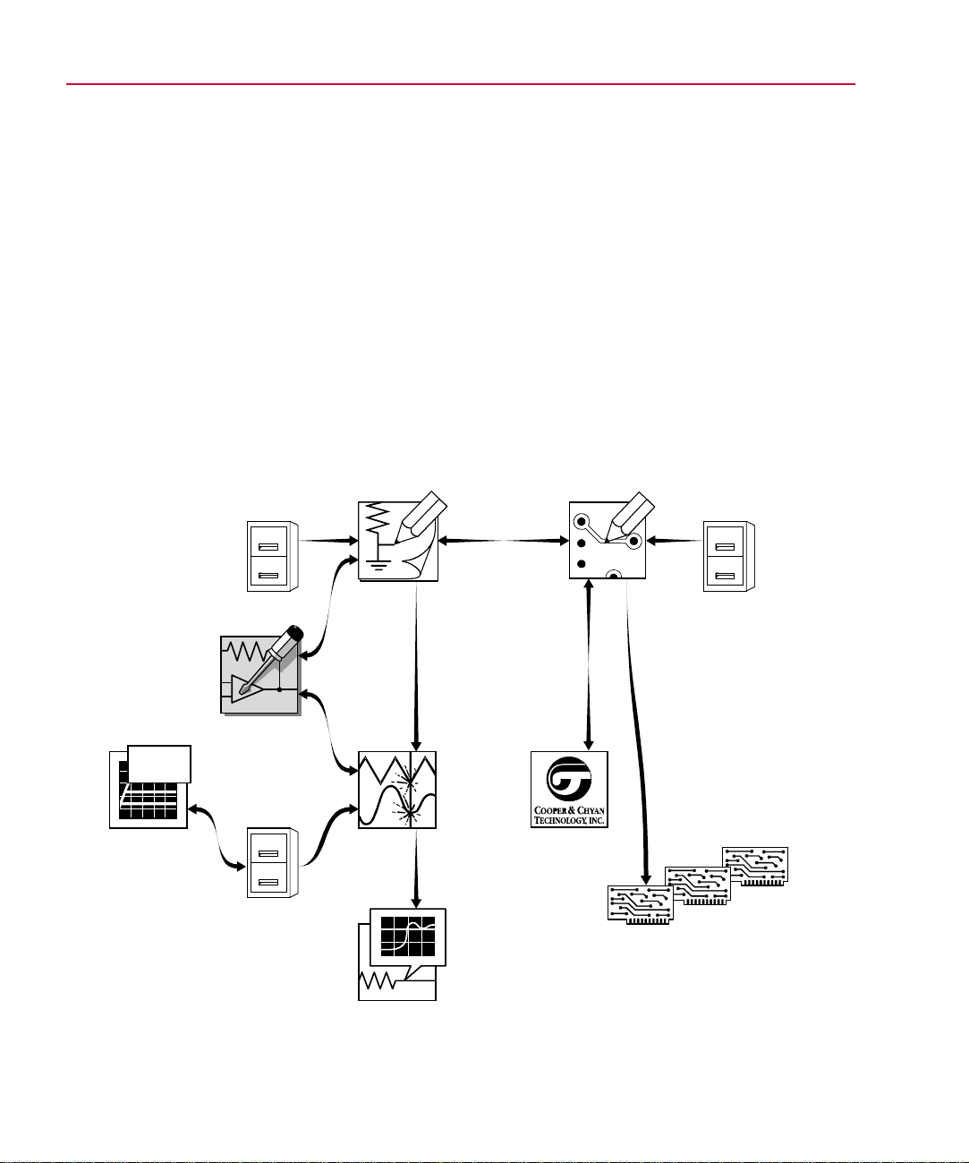
MicroSim PSpice Optimizer Overview

The MicroSim PSpice Optimizer is a circuit optimization program that improves the performance of analog and mixed analog/digital circuits. The PSpice Optimizer is fully integrated with other MicroSim programs. This means you can design your circuit with MicroSim Schematics, simulate with MicroSim PSpice A/D (or MicroSim PSpice), analyze results with MicroSim Probe and optimize performance within the same environment.

MicroSim PSpice Optimizer

MicroSim Parts

MODEL

+ BF =

symbols packages

models

MicroSim Schematics

MicroSim PSpice A/D

MicroSim Probe

MicroSim PCBoards

SPECCTRA Autorouter

packages footprints padstacks



reports

drill

Gerber

files

How to Use this Guide

This guide is designed so you can quickly find the information you need to use the PSpice Optimizer.

How to Use this Guide xv

This guide assumes that you are familiar with Microsoft Windows (NT or 95), including how to use icons, menus, and dialog boxes. It also assumes you have a basic understanding about how Windows manages applications and files to perform routine tasks, such as starting applications and opening, and saving your work. If you are new to Windows, please review your Microsoft Windows User’s Guide.

Typographical Conventions

Before using the PSpice Optimizer, it is important to understand the terms and typographical conventions used in this documentation.

This guide generally follows the conventions used in the Microsoft Windows 95 User’s Guide. Procedures for performing an operation are generally numbered with the following typographical conventions.

Notation Examples Description

ALL CAPS ANALOG.SLB or

CLIPPER.SCH

Library files and file names.

For UNIX users: All screen captures in this

manual are of Windows 95

boxes and windows.

dialo Most options in these dialo boxes and windows are available in your operatin environment. When certain options are not available to you, or you must do somethin differently than what is primarily outlined, information specific to your platform is provided.

Press C+

Type

... Commands/text entered from

VAC

C+r

monospace font

Notation Examples Description

A specific key or key stroke on the keyboard.

the keyboard.

xvi Before You Begin

If You Have the Evaluation Version

The evaluation version of the PSpice Optimizer has the following requirements and limitations:

• Requires the MicroSim PSpice A/D with Schematics

evaluation package.

• Is limited to one goal, one parameter, and one constraint.

Things You Need to Know

Chapter Overview

This chapter introduces the purpose and function of the PSpice Optimizer, the optimization process, and related terms.

What is the PSpice Optimizer?

capabilities and the criteria designs must meet for successful optimization.

Using the PSpice Optimizer with Other MicroSim Programs page 1-4 presents the high-level design flow for optimization

and how other MicroSim programs are integrated into each design phase.

Terms You Need to Understand

that are important for optimizing designs successfully.

on page 1-2 describes optimizer

on page 1-5 defines the terms

1-2 Things You Need to Know

What is the PSpice Optimizer?

The MicroSim PSpice Optimizer is a circuit optimization program that improves the performance of analog and mixed analog/digital circuits.

Run optimizations

iterative simulations, while adjusting the values of design parameters until performance goals, subject to specified constraints, are nearly or exactly met. Constraints can include simple bounds on parameter values and nonlinear functions. The PSpice Optimizer also computes Lagrange multipliers that provide information on the cost of each constraint on the solution.

Explore performance tradeoffs

values for design parameters, the PSpice Optimizer provides graphical feedback showing performance. You can also tweak goal and constraint values to examine changes to parameter values.

Fit model parameters

set of measured data points, and a good starting point for the parameter values, the PSpice Optimizer fits a more accurate model.

The PSpice Optimizer performs

When you enter new

Given a parameterized model, a

Designs that You Can Optimize

What is the PSpice Optimizer? 1

-3

A design that you can optimize must meet the following criteria:

• It works; that is, it simulates with PSpice to completion and

behaves as intended.

• One or more of its components have a variable value, and

each value that is varied relates to an intended performance goal.

• An algorithm exists to measure its performance as a

function of the variable value.

If you can visualize what factors should be adjusted to improve performance, and how you would manually step through the optimization process (even though the computations might seem unwieldy), then the design is a good candidate for the PSpice Optimizer.

Designs that You Cannot Optimize

You cannot use the PSpice Optimizer to:

Optimization problems are not always solvable by a particular

orithm.

• Create a working design. This especially applies when you

begin with a design that is far from meeting specifications.

• Optimize a design in which the circuit has several states

where a small change in a parameter value causes a change of state.

Example: A flip-flop is on for some parameter value, and off for a slightly different value.

1-4 Things You Need to Know

Using the PSpice Optimizer with Other

Because you can use Schematics, PSpice, and Probe to desi system, subcircuit, or component level, use the PSpice Optimizer to optimize at whatever level is most appropriate.

n and simulate at the

MicroSim Pro

rams

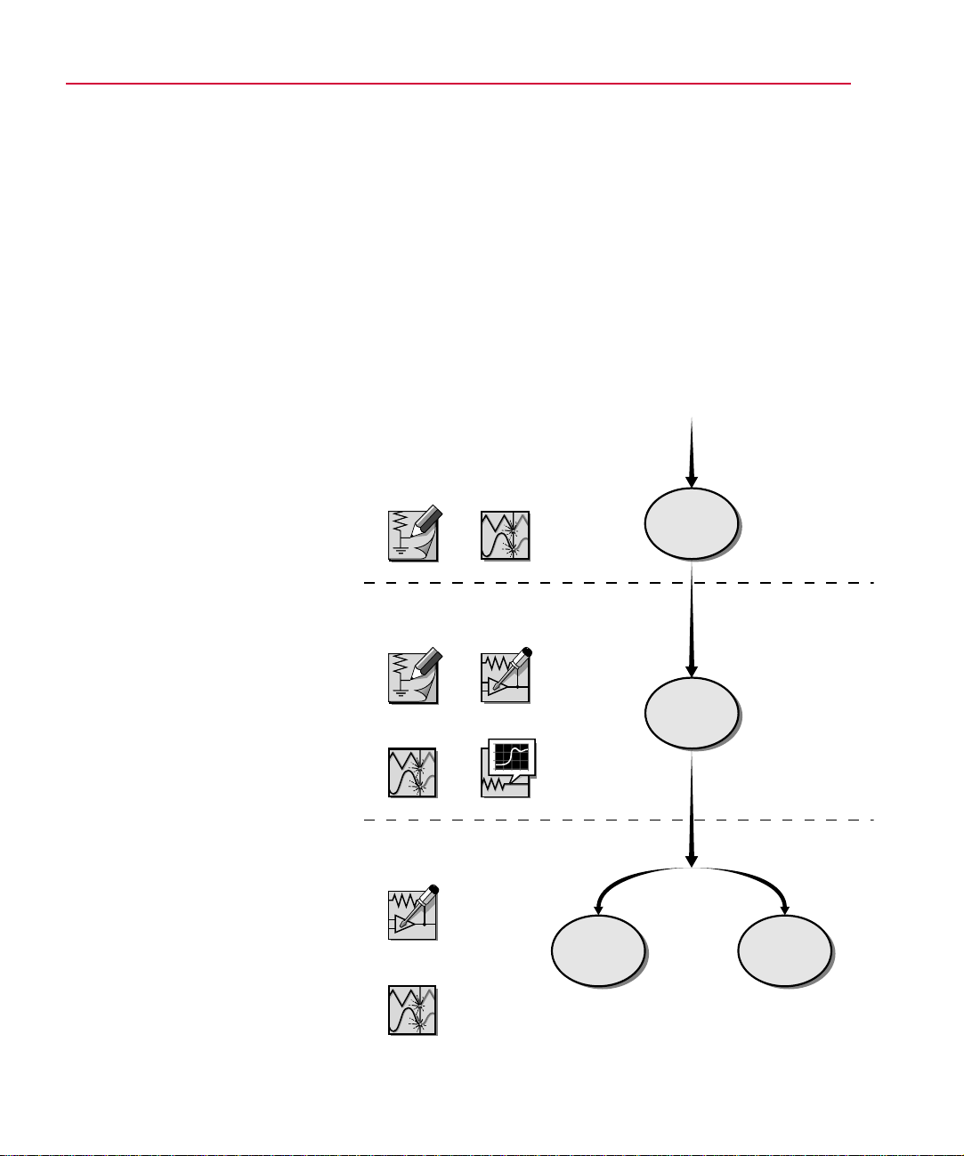
The PSpice Optimizer is fully integrated with other MicroSim programs. This means you can design your circuit with MicroSim Schematics, simulate with MicroSim PSpice A/D (or MicroSim PSpice), analyze results with MicroSim Probe and optimize performance within the same environment. Figure 1-1 illustrates the typical design flow for circuit optimization.

Phase One

MicroSim Schematics

MicroSim PSpice A/D

MicroSim PSpice Optimizer

MicroSim Probe

Develop

the

Design

Phase Two

Set Up

the

Optimization

See Chapter 2, “Primer: How to

Optimize a Design

description of each desi phase.

” for a detailed

ure 1-1

MicroSim PSpice Optimizer

MicroSim PSpice A/D

Run

the

Optimization

Optimization Design Flow

Phase Three

Fit

Model

Parameters

Terms You Need to Understand

Terms You Need to Understand 1

-5

Optimization

Optimization is the process of fine-tuning a design by varying design parameters between successive simulations until performance comes close to (or exactly meets) the ideal performance.

The PSpice Optimizer solves four types of optimization problems as described in Table 1-1.

Table 1-1

Problem Type PSpice Optimizer Action Example

unconstrained minimization reduces the value of a single goal minimize the propagation delay

constrained minimization reduces the value of a single goal while

unconstrained least squares

constrained least squares reduces the sum of squares of the

Optimization Problems

satisfying one or more constraints

reduces the sum of the squares of the individual errors (difference between the ideal and the measured value) for a set of goals

individual errors for a set of goals while satisfying one or more constraints

through a logic cell minimize the propagation delay

through a logic cell while keeping the power consumption of the cell less than a specified value

given a terminator design, minimize the sum of squares of the errors in output voltage and equivalent resistance

minimize the sum of squares of the figures of merit for an amplifier design while keeping the open loop gain equal to a specified value

*. All four cases allow simple bound constraints; that is, lower and upper bounds on all of the parameters. The PSpice Optimizer also handles nonlinear goals and constraints. **. Use unconstrained least squares when fitting model parameters to a set of measurements, or when minimizing more than one goal.

1-6 Things You Need to Know

See Chapter 6,Tutorial:

Exploring Design Tradeoffs (Active Filter) startin

6-1 for a workin

showin values.

For more information, see and

parameterized slider

Constraint on page 1-8.

on page

example

Goal

Parameter

A parameter defines a property of the design for which the PSpice Optimizer attempts to determine the best value within specified limits. A parameter can:

• Represent component values (such as resistance, R, for

a resistor).

• Represent other component attribute values (such as

slider settings in a potentiometer).

• Participate in expressions used to define component

values or other component attribute values.

The PSpice Optimizer can optimize designs with up to eight variable parameters.

Example: A potentiometer symbol in a schematic uses the SET attribute to represent the slider position. You can assign a parameterized expression to this attribute to represent variable slider positions between 1 and 0. During optimization, the PSpice Optimizer varies the parameterized value of the SET attribute.

Specification

A specification describes the ideal behavior

of a design in terms of goals and constraints. Examples: For a given design, the gain shall be 20 dB ±1 dB; for

a given design, the 3 dB bandwidth shall be 1 kHz; for a given design, the rise time must be less than 1 usec.

A design can have up to eight goals and constraints in any combination, but there must always be at least one goal. You can easily change a goal to a constraint and vice-versa.

The PSpice Optimizer accepts specifications in two formats: internal and external.

Internal specifications

An internal specification is composed of goals and constraints defined in terms of target values and ranges, which are entered into the PSpice Optimizer through dialog boxes.

External specifications

An external specification is composed of measurement data, which are defined in an external data file that is read by the PSpice Optimizer.

Terms You Need to Understand 1

-7

Target value

A target value is the ideal operating value for a characteristic of the design as defined by a goal or constraint specification.

Goal

A goal defines the performance level that the design should attempt to meet (e.g., minimum power consumption). A goal specification includes:

• The name of the goal.

• A target value and an acceptable range.

• A circuit file to simulate.

• An evaluation for measuring performance.

• An analysis type used for simulation-based evaluations.

The goal specification can also include:

• The name of the file containing Probe goal function

definitions (.prb file).

• When using an external specification, the name of the file

containing measured data and the columns of data to be used as reference.

Typically, the PSpice

Note

Optimizer measures performance usin

an evaluation that requires a simulation, and therefore, you must specify the circuit file for the simulation. However, when measurin

PSpice Optimizer

usin

performance

expressions which do not require a simulation, you do not need to specify a circuit file.

1-8 Things You Need to Know

Constraint

A constraint defines the performance level that the design must fulfill in which the target value exceeds, falls below, or equals a specified value (e.g., an output voltage that must be greater than a specific level). The constraint specification includes:

• The name of the constraint.

• A target value and an acceptable range.

• A circuit file to simulate. (See note on previous page.)

• An evaluation for measuring performance.

• An analysis type used for simulation-based evaluations.

• An allowed relationship between measured values and the

target value, which can be one of the following: <= measured value must be less than or equal

to the target value = measured value must equal the target value >= measured value must be greater than or

equal to the target value

The constraint specification can also include the name of the file containing Probe goal function definitions (.prb file).

See Optimization on page 1-5 for more on least-squares and minimization al

orithms.

Constraints are often nonlinear functions of the parameters in the design.

Example: Bandwidth can vary as the square root of a bias current and as the reciprocal of a transistor dimension.

Performance

The performance of a design is a measure of how closely its specifications’ calculated values approach their target values for a given set of parameter values. When there are multiple specifications (at least one of which is a goal), the PSpice Optimizer uses the sum of the squares of their deviations from target to measure closeness. For a single specification (goal), the PSpice Optimizer uses either the goal’s value, or the square of its deviation from target.

Each aspect of a design’s performance is found by either:

• first performing the appropriate simulation, then running

Probe to measure characteristics of the resulting waveform(s), or

• evaluating PSpice Optimizer expressions.

In many cases (particularly if there are multiple conflicting specifications), it is possible that the PSpice Optimizer will not meet all of the goals and constraints. In these cases, optimum performance is the best compromise solution—that is, the solution that comes closest to satisfying each of the goals and constraints, even though it may not completely satisfy any single one.

Terms You Need to Understand 1

-9

Evaluation

An evaluation is an algorithm that computes a single numerical value, which is used as the measure of performance with respect to a design specification.

The PSpice Optimizer accepts evaluations in one of these three forms:

• single-point Probe trace function

• Probe goal function

• PSpice Optimizer expression

Given evaluation results, the PSpice Optimizer determines whether or not the changes in parameter values are improving performance, and determines how to select the parameters for the next iteration.

Trace function

A trace function defines how to evaluate a design characteristic when running a single-point analysis (such as a DC sweep with a fixed voltage input of 5 V).

Examples: V(out) to measure the output voltage; I(d1) to measure the current through a component.

Refer to the online MicroSim

PSpice A/D Reference Manual

for the variable formats and mathematical functions you can use to specify a trace function.

1-10 Things You Need to Know

Refer to the Goal Function wizard in Probe user’s how to develop and specify functions.

Here are some quick tips. In Probe:

• To test the value returned by

• To see the waveforms and

See Gain on page 7-5 for an example of the YatX function definition.

uide for information on

a specified select Eval Goal Function from the Trace menu.

marked points used to evaluate a select Display Evaluation in the Probe Options dialo (from the Tools menu, select Options to display this dialo box).

and your PSpice

oal

oal function,

box

oal

Probe goal function

A Probe goal function defines how to evaluate a design characteristic when running any kind of analysis other than a single-point sweep analysis. A goal function computes a single number from a Probe waveform. This can be done by finding a characteristic point (e.g., time of a zero-crossing) or by some other operation (e.g., RMS value of the waveform).

For example, you can use Probe goal functions to:

• Find maxima and minima in a trace.

• Find distance between two characteristic points (such as

peaks).

• Measure slope of a line segment.

• Derive aspects of the circuit’s performance which are

mathematically described (such as 3 dB bandwidth, power consumption, and gain and phase margin).

To write effective goal functions, determine what you are attempting to measure, then define what is mathematically special about that point (or set of points).

Note

Be sure that the goal functions accurately measure what they are intended to measure. Optimization results hi functions behave. Discontinuities in

hly depend on how well the goal

oal functions (i.e., sudden jumps for small parameter chan can cause the optimization process to fail.

es)

PSpice Optimizer expression

A PSpice Optimizer expression defines a design characteristic. The expression is composed of optimizer parameter values, constants, and the operators and functions shown in Table 1-2.

Example: To measure the sum of resistor values for two resistors with parameterized values named R1val and R2val, respectively, use the PSpice Optimizer expression R1val + R2val.

Terms You Need to Understand 1

-11

Table 1-2

Valid Operators and Functions for PSpice

Optimizer Expressions

Operator Meanin

+ addition

- subtraction * multiplication / division ** exponentiation exp e log ln(x) log10 log sin sine cos cosine tan tangent atan arctangent

Note

Unlike trace functions and Probe goal functions,

(x)

PSpice Optimizer expressions are evaluated without usin

a simulation or Probe.

Derivative

A derivative defines mathematically how a specification value changes with a small change in parameter value.

For a given design, the PSpice Optimizer calculates derivatives for each specification with respect to each parameter. Within an applicable range, the optimizer uses the derivatives to estimate new values for the goals and constraints.

See Derivatives on page 4-10 for a detailed discussion.

Primer: How to Optimize a

Desi

Chapter Overview

This chapter guides you through the basic steps needed to setup and run an optimization using a simple diode biasing design.

Optimizing a Diode Biasing Circuit—the Objective

describes the sample circuit and its ideal operating characteristics.

on page 2-2

Why Use Optimization?

your design using the PSpice Optimizer saves time.

Phase One: Developing the Design

through the steps needed to create a working design.

Phase Two: Setting Up the Optimization

through the steps needed to define the parameters, goals, and constraints that describe the optimization.

Phase Three: Running an Optimization

through the steps needed to optimize and finalize the design.

on page 2-3 explains why fine-tuning

on page 2-4 walks you

on page 2-6 walks you

on page 2-11 walks you

2-2 Primer: How to Optimize a Design

Optimizing a Diode Biasin Ob

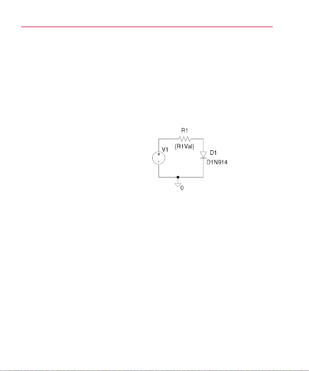
Assume that you want to design a circuit that drives a current of 1 mA (±5 µA) through a diode (D1N914) using a 5 Vvoltage source and a series resistor to control the current through the diode. A circuit such as this is shown in Figure 2-1.

Your objective is to find a value for resistor R1 so that current through diode D1 falls in the range 0.995 mA to 1.005 mA.

ective

ure 2-1

Circuit—the

Diode Biasing Design Example

Why Use Optimization?

Why Use Optimization? 2

-3

To solve the problem manually, you could assign an arbitrary value to R1, manually calculate the current, then make an educated guess to adjust the values until a satisfactory solution is found. Or, you might use a simulation to sweep the value for R1 with a DC Sweep analysis, carefully analyzing the results to find the best solution.

These manual methods have two major disadvantages:

• Because the diode is a non-linear device, manual

calculations can be time-consuming.

• Sweeping a parameterized value can take a large number of

simulations, depending on the range and increment selected.

The PSpice Optimizer automates these processes by handling calculations for you and intelligently directing the series of simulations. Given results of the previous simulations, the optimizer automatically adjusts the parameterized value of R1 for the next run, thus eliminating unnecessary iterations, which in turn, provides a solution more quickly and with less effort.

Once the PSpice Optimizer settles on the best solution, you can still explore available tradeoffs. When done manually, this iterative process can be difficult and frustrating. With the optimizer, you can tweak the parameter(s) and immediately determine whether the design still meets specifications. You can also change the value of the specification(s) and immediately determine how parameter values change. If you are dissatisfied with the result after any change, you can always return to the last set of values.

When solving complex problems, the manual approach can be too unwieldy to consider. For example:

• When your desi

multiple parameters or complicated parameter interactions, you may find it’s nearly impossible to know which parameters to chan and how best to chan them.

• When solvin

specifications, the solution often depends on the order in which are optimized. This sequential approach can miss possible solutions since it is impractical to repeat the process startin different each time.

oals and constraints

oal or constraint

n has

for multiple

with a

2-4 Primer: How to Optimize a Design

Phase One: Developing

Phase 1 is also the time to investi

• The effects of individual

• Usin

ate:

components by replacin component values with parameters or parameterized expressions.

PSpice to perform a DC, AC, or parametric sweep of each parameterized value.

the Desi

Before optimizing, you must have a working circuit. This means first drawing the schematic, then iteratively simulating with PSpice and adjusting the design until the circuit operates with the intended behavior.

MicroSim Schematics

MicroSim PSpice A/D

Design

Schematic

Simulate

Note

resistor R1, its value is 1k. Later, when you set up the optimization, you will parameterize R1’s value as shown in Fi

When you initially place

ure 2-1.

Flow

ure 2-2

“Phase One: Developing the Design” Design

To draw the schematic for the diode biasing desi

In Schematics, from the Draw menu, use Get New Part to select and place the following symbols on the schematic:

R resistor R1 D1N914 diode D1 VSRC voltage source V1 AGND analog ground 0

Phase One: Developing the Design 2

From the Draw menu, use Wire to connect the symbols as

shown in Figure 2-1. From the Edit menu, use Attributes to set V1’s DC attribute

5v.

to From the File menu, select Save As and enter

mydiode.sch in the File Name text box.

The PSpice Optimizer Advantage

To determine a value for R1 manually, you can set up a parametric analysis of a DC sweep where:

• the value of R1 steps from 4 k to 5 k in increments of 0.1 k,

and

• the DC sweep analysis is a single-point voltage analysis at 5

Such an analysis requires eleven PSpice simulations. Using Probe, the resistor value giving rise to 1 mA current through D1 is 4.14 k.

-5

The remainder of this chapter shows how to use the PSpice Optimizer to determine the same solution automatically using fewer simulations.

2-6 Primer: How to Optimize a Design

Phase Two: Setting Up the Optimization

Now that preliminary design development is complete, you are ready to define the optimization parameters, goals, and constraints.

MicroSim Schematics

Define Design

Parameters

Set Up

Analyses

MicroSim PSpice A/D

MicroSim PSpice Optimizer

ure 2-3

Flow

MicroSim Probe

Develop

Performance

Measures

Define

Goals &

Constraints

Simulate

“Phase Two: Setting Up the Optimization” Design

Phase Two: Setting Up the Optimization 2

Defining Design Parameters

To define parameters for optimization, you must:

• Identify the parameters to adjust for optimization and assign

a unique name to each one.

-7

• Set up each parameter as a global optimization parameter

using the Schematic Editor and the OPTPARAM symbol.

• Select which components in the design are affected by the

parameter and, for each component, replace its value (e.g., the value of its VALUE attribute) with an expression that includes the parameter name.

To prepare the diode design example for optimization, you need to parameterize the value of R1 and specify its optimization properties.

To set up the value of R1 as a parameter named R1Val

In Schematics, from the Draw menu, use Get New Part to

place an instance of the OPTPARAM symbol (from

special.slb).

Double-click on the OPTPARAM symbol, then set R1val

properties as shown in the Optimizer Parameters dialog box.

You can also define optimization parameters in the PSpice Optimizer by selectin Parameters from the Edit Menu.

Adding and Editing

See

Parameters on page 3-10 for

more information.

The parameter settings are: Name = R1Val Initial Value= 5k Current Value= 5k Lower Limit= 100 Upper Limit= 10K

Click OK.

Double-click the 1k label for R1 and enter

parameterize the value of R1. Click OK.

Tolerance= 10% Later, in Schematics, when you

select Run Optimizer from the Tune menu, the parameters specified with the OPTPARAM symbol are loaded into the PSpice Optimizer and displayed in its main window.

{R1val} to

2-8 Primer: How to Optimize a Design

Setting Up Goals and Constraints

Before you can evaluate and improve the circuit’s performance, you must answer these questions:

• What operating characteristics do I want to measure?

• How do the parameters affect the operating characteristics?

Once you’ve answered these questions, you are ready to:

• Set up the analyses needed to evaluate the performance

• Develop the performance measure algorithms.

• Fully define the goals and constraints in terms of these

Setting up analyses for each goal and constraint

For each specification, you must define an analysis type: AC, DC, or transient. This is the analysis that PSpice will run to generate results used by the PSpice Optimizer to measure performance.

measures.

performance measures and analyses.

For the diode design example, you want to monitor the value of I(D1) at a fixed input voltage of 5 V while the optimization parameter, R1val, is varied. This means setting up a single-point voltage sweep.

To set up a single-point voltage sweep analysis at 5 volts

In Schematics, from the Analysis menu, select Setup.

In the Analysis Setup dialog box, select the DC Sweep

check box.

To fix the voltage of V1, fill in the DC Sweep dialog

box as shown.

Click OK to return to the Setup Analysis dialog box.

Select the DC Sweep check box to enable it.

Clear all other analysis check boxes.

Click OK.

Phase Two: Setting Up the Optimization 2

The DC Sweep settings are: Swept Var Type = Volta

Source Sweep Type= Value List Name = V1 Values = 5v

-9

Developing performance measures

To measure performance you must define an evaluation algorithm for each specification. There are three alternatives:

• trace function (for single-point simulations)

• Probe goal function

• PSpice Optimizer expression

When the evaluation is anything other than a single-point simulation or PSpice Optimizer expression, you must develop Probe goal functions to derive values from the simulation results. Developing goal functions is an iterative process that involves writing the goal function, simulating the design, and testing the goal functions against actual results to make sure you are measuring the waveform characteristics you intended.

A Probe goal function is not required for the diode design example. You are examining the trace of R1Val versus I(D1) which shows the relationship between the value of R1 and the diode forward current. Because only a single point on the curve is of interest, the trace function, I(D1), is the appropriate evaluation.

See Evaluation on page 1-9 and the sections that follow for a definitions of trace function, Probe Optimizer expression.

MicroSim supplies standard goal functions for AC, DC, and transient analyses in the file msim.prb. This file resides in the MicroSim root directory. You can add create a local .prb file for use with a specific desi

See

oal function, and PSpice

oal functions to this file, or

Chapter 7,Tutorial: Using

Constrained Optimization (MOS Amplifier) for examples of

Probe evaluate performance.

Refer to your PSpice user’s

description of the local .prb files.

oal functions used to

uide for instructions on creating oal functions, and for a

lobal and

2-10 Primer: How to Optimize a Design

Defining specifications: goals and constraints

Now that you’ve completed the preliminary groundwork, you are ready to define the properties for goals and constraints. So far, you have performed all steps in Schematics. To finalize setup, you must specify the goal for the diode design example using the PSpice Optimizer.

To define the design goal, Id1, for the diode desi

3 4

n example

In Schematics, from the Tools menu, select Run Optimizer to activate the PSpice Optimizer.

The PSpice Optimizer window appears showing the parameter R1val that you defined using the OPTPARAM symbol in the schematic.

In PSpice Optimizer, from the Edit menu, select Specifications.

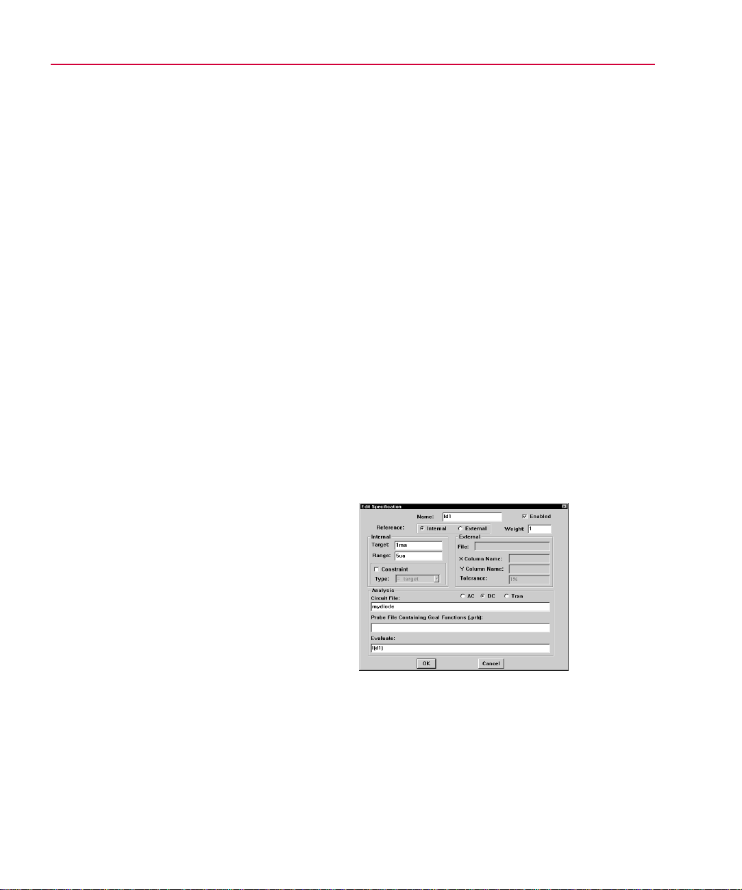
In the Specifications dialog box, click Add. Enter Id1 properties as shown in the following Edit

Specification dialog box.

The goal specification settings are:

Name = Id1

et = 1ma

Tar

e= 5ua

Ran Analysis= DC Circuit File= mydiode Evaluate= I(d1) The PSpice Optimizer

appropriately defaults to the internal specification settin shown in the Reference control.

Phase Three: Running an Optimization 2

Phase Three: Running an Optimization

Now that you have defined the parameters, specifications, and evaluations for the design, you are ready to optimize, adjust, and finalize your design.

MicroSim PSpice Optimizer

Optimize Simulate

ust

Specifications

-11

MicroSim PSpice A/D

MicroSim Probe

Standardize

Component

Values

Save

Results

Generate

Reports

Update

the

Schematic

Improved

Design

ure 2-4

“Phase Three: Running an Optimization” Design

Phase

2-12 Primer: How to Optimize a Design

Running the PSpice Optimizer

You can use the PSpice Optimizer to:

• Optimize the circuit to completion (from the Tune menu,

select Auto).

This is useful when initially validatin restartin adjustin specifications.

This is useful when exploring desi parameter and specification values.

the circuit or when

optimization after

parameters or

n tradeoffs by tweaking

• Evaluate performance for a single set of parameter values

(from the Tune menu, select Update Performance).

• Compute derivatives of each specification with respect to

each parameter (from the Tune menu, select Update Derivatives).

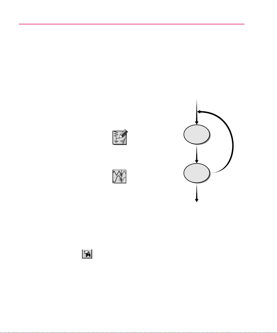
When you select Auto from the Tune menu, the PSpice Optimizer automatically computes the derivatives for each specification with respect to each parameter (Figure 2-5). Using the derivatives, the optimizer determines the direction in which to vary the parameters, and changes parameter values accordingly until it achieves a reduction in the overall error. After updating the parameters, the optimizer computes new derivatives and repeats the process until one of the following occurs:

• Specifications are met (success).

• No more progress can be made (failure).

• You manually interrupt the process.

Startin

Parameter

Values

Evaluate

Performance

Phase Three: Running an Optimization 2

-13

Compare to

Specifications

Evaluate

Derivatives

Compute

New

Parameter

Values

Satisfied?

Iteration Limit

Reached?

ence

Conver

Fails?

Yes

Done

ure 2-5

PSpice Optimizer Automatic Optimization Process

2-14 Primer: How to Optimize a Design

To start optimizing the diode design

In the diode example, the derivative at R1=5 k is –1.62 x 10

-7

, or

∂

Id() 1.62

R1∂

This indicates that a 1 ohm increase in R1 will produce a decrease of 0.162 uA in Id1. To verify this, try reducin of R1 by 100 ohms (to 4.9 kohm) and simulate. This increases the diode current by 16.2 uA and

rees with the derivative

a information.

See The PSpice Optimizer

7–

×10–=

the value

Window on page 3-5 for a

complete description of the window elements and how you can interact with them.

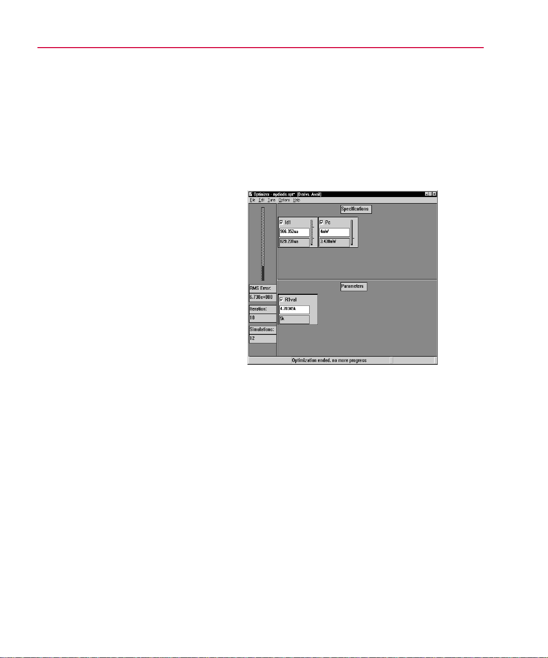
From the Tune menu, select Auto and click Start.

The PSpice Optimizer performs several simulations. For each iteration of the parameter values, the optimizer calculates overall performance and graphically displays the results. The optimizer also calculates the value of the trace function, I(d1), and displays the new value in the specifications area of the PSpice Optimizer window. After three iterations, the optimizer should converge on a solution of 4.131 K, as shown in Figure 2-6.

ure 2-6

Optimization Results for the Diode Design

Example

Adding a Constraint and Rerunning the PSpice Optimizer

So far, you have optimized for a single goal, Id1. Now suppose you want to add a condition, or constraint, on the power dissipated in resistor R1.

Constraints are defined like goals (using the Edit Specification dialog box) with two additions. In the Internal frame, you must:

• Select the Constraint check box.

• Choose the constraint type (>= target, = target, or, <=

target).

Phase Three: Running an Optimization 2

The constraint type specifies the required relation between what is evaluated (as defined in the Evaluate text box) and the target value (defined in the Target text box).

To define the constraint for power dissipation in R1

The power dissipated in R1 must be less than or equal to 4 mW±400 uW. Define the constraint by doing the following:

In PSpice Optimizer, from the Edit menu, select

Specifications. In the Specifications dialog box, click Add.

Enter the power (Pc) constraint properties as shown in the

following Edit Specification dialog box.

The constraint specification settin

s are:

Name = Pc

et = 4mW

Tar

e = 400uW

Ran Constraintselected

-15

Type = <=tar Analysis= DC Circuit File= mydiode Evaluate= i(r1)*v(r1:1,r1:2)

The Evaluate text box contains the expression for measuring dissipated power. For each iteration, Probe will compute dissipated power by taking the product of the voltage across the resistance and the current through it.

To calculate the performance of the design for initial

parameter and specification values only (one iteration):

From the Edit menu, select Reset Values.

From the Tune menu, select Update Performance.

Note the appearance of the progress indicator in the Pc box. Since Pc is a less than or equal to constraint, the

See Progress indicator on

page 3-7 for more on the

different kinds of pro indicators and how to interpret them.

progress indicator

ress

2-16 Primer: How to Optimize a Design

progress indicator has a tick mark 1/4 of the way up. The vertical bar within the indicator is below the tick mark; this means that the constraint is currently satisfied.

From the Tune menu, select Auto and click Start to start optimization.

After a number of iterations, the optimization ends without satisfying the goal.

ure 2-7

Note that the power dissipated in R1 is exactly equal to the target value of the constraint (4 mW). In this example there is no feasible solution to the problem. However, the PSpice Optimizer found the lowest value for Id1 which does not violate the constraint.

Results after Adding the Power Constraint

Changing the Constraint and Rerunning the PSpice Optimizer

You can examine the effect the Pc constraint has on performance by changing its constraint type so the power dissipation in the resistor must be greater than or equal to 4mW.

Phase Three: Running an Optimization 2

To change the Pc constraint type to “greater than or equal”

In PSpice Optimizer, double-click the lower right-hand

corner of the Pc box. In the Edit Specifications dialog box, change Type to >=

target. Click OK.

To run the optimization with the modified constraint

Test performance with the updated constraint:

From the Edit menu, select Reset Values.

From the Tune menu, select Update Performance.

The Pc constraint is initially violated because the power dissipation is less than 4 mW.

From the Tune menu, select Auto and click Start to start

optimization.

-17

double-click here

The PSpice Optimizer finds a solution which satisfies both the goal (current of 1 mA) and the constraint (power dissipated in the resistor greater than 4 mW). Figure 2-8 shows the results.

ure 2-8

Results after Changing the Constraint Type

2-18 Primer: How to Optimize a Design

Using Standard Component

See Using Standard Component

Values on page 3-29 for more

information, includin PSpice Optimizer uses tolerances and limits when standardizin

values.

rounded resistor value

how the

Values

When an optimization completes successfully, the optimizer displays the new parameter values in the PSpice Optimizer window. However, each calculated value might not correspond to an actual value that is available with off-the-shelf components. For example, resistors are not readily available in all possible values.

You can use the PSpice Optimizer to select standard component values. The optimizer either:

• rounds to the nearest value, or

• computes values based on the most recent optimization run.

To round to the nearest standard component value

From the Edit menu, select Round Nearest.

R1val’s current value changes to 3.9 k in accordance with the specified 10% tolerance.

Producing Reports

You can use the PSpice Optimizer to generate a report summarizing:

• current settings for parameter, specification, and program

options.

• calculated derivatives and Lagrange multipliers.

To generate a summary report

From the File menu, select Report.

The PSpice Optimizer writes the final results to

mydiode.oot as shown in Figure 2-9.

Phase Three: Running an Optimization 2

-19

ure 2-9

Report Summary for the Diode Optimization

Saving Results

When you have finished optimizing, you can save all of the optimizer data, including the current values for all parameters and specifications.

To save the optimizer data for the diode design

From the File menu, select Save.

The PSpice Optimizer updates the of the options settings are also saved.

mydiode.opt file. All

Updating the Schematic

Having completed the optimization, you can update the data in the schematic file to include the optimized parameter values.

2-20 Primer: How to Optimize a Design

To update the diode schematic with the current parameter values

From the Edit menu, select Update Schematic. Recall that R1Val was initially set at 5.0 k in the schematic

file. When you select Update Schematic, the PSpice Optimizer sends a message to Schematics to update the schematic file. Schematics writes the new parameter value of 3.9 k to the OPTPARAM symbol on the schematic (as the current value).

Figure 2-10 shows the updated schematic for the diode design.

ure 2-10

Updated Diode Schematic

Using the PSpice Optimizer

Chapter Overview

This chapter describes in general terms how to complete any task using the PSpice Optimizer, including:

• How to activate the PSpice Optimizer and load a design,

page 3-2

• How to interact with the PSpice Optimizer window,

page 3-5

• How to add and edit optimization parameters, page 3-10.

• How to add and edit goals and constraints, page 3-13.

• How to measure and optimize performance, page 3-18.

• How to explore design tradeoffs, page 3-20.

• How to generate result summaries including Lagrange

multipliers and derivative values, page 3-26

• How to finalize the design: standardize component values,

save results, and back-annotate the schematic, page 3-26

3-2 Using the PSpice Optimizer

Activating and Loading the PSpice Optimizer

This section describes how to:

• Start the PSpice Optimizer.

• Set special startup options.

• Load a design.

Activating the PSpice Optimizer

Start the PSpice Optimizer program either from:

• Schematics, or

• the Windows 95 Start menu.

Tools menu

From Schematics To activate the PSpice Optimizer from

Schematics

In Schematics, from the Tools menu, select Run Optimizer.

If you have an active schematic loaded into the Schematic Editor when you select Run Optimizer, any optimization parameters defined with the OPTPARAM symbol and any existing setup information contained in the corresponding optimization file ( PSpice Optimizer.

If no schematic is active, the PSpice Optimizer activates without an optimization setup. Instead, you must load an optimization file directly into the optimizer as described in

Loading a Different Optimization File

.opt) are automatically loaded into the

on page 3-4.

Activating and Loading the PSpice Optimizer 3

From the Windows 95 Start Menu

From the Windows 95 Start menu, there is a program folder which contains Windows 95 shortcuts for all installed MicroSim programs, including the PSpice Optimizer.

-3

To activate the PSpice Optimizer from the Windows 95 Start menu

From the Windows 95 Start menu, select the MicroSim

program folder and then the PSpice Optimizer shortcut to start optimizer.

The optimizer activates without an optimization setup. See

Loading a Different Optimization File

on page 3-4 for

further instructions.

Changing Activation Options

The PSpice Optimizer supports two command line options, which are used to:

• Activate the optimizer with an initialization file other than

the default (

• Automatically load an optimization file (.opt) after startup.

You can add one or both options to the command line.

To change the initialization file used by the PSpice Optimizer

In the optimizer command line, use the -i option as follows:

OPTIMIZE -i

msim.ini).

initialization_file_name

For UNIX users: To activate the PSpice Optimizer

on UNIX platforms, either double-click on the optimization file (.opt) in the File Mana window, or type “optimize” within a Shelltool window.

Because you can activate the PSpice Optimizer from either Schematics or from the Windows 95 Start menu, we recommend

that you chan occurrences of the command line definitions as follows:

• Use a text editor to open the

msim.ini file and, in the [MICROSIM OPTIONS] section, chan OPTIMIZECMD line.

• In the Windows Explorer,

e the Target text box in

chan the optimizer’s Properties

box (click once on the

dialo PSpice Optimizer shortcut, then, from the File menu, select Properties and click the Shortcut tab).

both

e the

3-4 Using the PSpice Optimizer

To automatically load an optimization file after startup

In the PSpice Optimizer command line, add the name of the

optimization file as follows:

OPTIMIZE

The following command line example shows how to start the optimizer at all times with an initialization file named

myinit.ini and an optimization file named mydesign.opt:

OPTIMIZE mydesign.opt -i myinit.ini

optimization_file_name

Loading a Different Optimization File

Once you have activated the PSpice Optimizer, you can change to a new or different optimization file at any time.

To start a new optimization

From the File menu, select New.

To load an existing optimization setup

From the File menu, select Open.

Locate and select the appropriate optimization file.

The PSpice Optimizer

Window

The PSpice Optimizer window contains three areas:

• specifications area

• parameters area

• error gauge area

Figure 3-1 illustrates their position in the window.

The PSpice Optimizer Window 3

-5

error gauge area

ure 3-1

specifications area

parameters area

The PSpice Optimizer Window

3-6 Using the PSpice Optimizer

Specifications Area

The specifications area can show up to eight specification boxes where each box represents either a goal or a constraint. Figure 3-2 illustrates the fields contained in each box.

enable/disable check box

progress indicator

current value

edit specification hot spot

initial value

For more information on the enable/disable check box, see

Excluding Parameters and Specifications from Optimization on page 3-24. For

more information on the edit hot spot, see

Selecting a

Specification to Edit on page 3-18.

If derivative data is available, you can chan to explore how parameter values mi

e the value in this field

ht change. See Testing

Performance when Changing Current Values on page 3-21 for

more information.

ure 3-2

Example of a Specification Box

The contents of the box varies depending on the source for the specifications—either internal or external. The following sections describe the differences in the initial and current value fields, and the progress indicator.

Internal specifications

Initial value

performance measure that the PSpice Optimizer sets when you start an optimization. The optimizer derives this value from the initial optimization parameter values you defined in the schematic (or the optimizer).

Current value

performance measure that corresponds to the current parameter values. Current values are updated each time an optimization iteration makes progress. When the current value satisfies the specification (that is, the current value is within the allowed range of the target) then the progress indicator turns from red to green, and the PSpice Optimizer considers the specification satisfied.

The initial value field displays a single

The current value field displays the

The PSpice Optimizer Window 3

-7

Progress indicator

As mentioned above, the progress indicator shows red while the specification is violated, and changes to green when the specification is satisfied.

You can monitor progress as the optimization runs by watching the progress indicator and observing the height of the vertical black bar relative to the tick mark(s) to the right. The number and relative position of the tick mark(s) varies depending on the type of specification:

• Two tick marks for a goal or equality constraint denote the

acceptable range around the target value.

• A single tick mark one-quarter of the way up denotes a less

than or equal to constraint.

• A single mark three-quarters of the way up denotes a

greater than or equal to constraint.

External specifications

Initial value

way from an internal specification: the field contains a pair of numbers separated by a ‘/’ character. The first number is the number of subgoals in the external specification that are satisfied. The second number is the total number of subgoals in the external specification.

The initial value field is used in a different

oal or equalit

constraint

less than or equal to constraint

reater than or

equal to constraint

Current value

The current value field is used in a different way from an internal specification: the field contains a pair of numbers as described above for initial value.

Progress indicator

The progress indicator shows the fraction of subgoals that are satisfied. The indicator turns from red to green when all of the subgoals are satisfied.

Example: If an external specification has 20 subgoals and five are satisfied, the current value field reads

5/20 and the bar in the

progress indicator rises to the one-quarter mark.

3-8 Using the PSpice Optimizer

Parameters Area

The parameters area can show up to eight parameter boxes. Figure 3-2 illustrates the fields contained in each box.

enable/disable check box

current value

edit parameter hot spot

initial value

For more information on the enable/disable check box, see

Excluding Parameters and Specifications from Optimization on page 3-24. For

more information on the edit hot spot, see

Selecting a Parameter

to Edit on page 3-12.

If derivative data is available, you can chan to explore how specification values mi

e the value in this field

ht change. See

Testing Performance when Changing Current Values on page 3-21 for more information.

ure 3-3

Example of a Parameter Box

The following sections explain the initial and current value fields in the parameter box.

Initial value

The initial value field displays a single value taken from the parameter specification that you set up either in Schematics (using the OPTPARAM symbol) or in the PSpice Optimizer (from the Edit menu, select Parameters).

Current value

Initially, the current value is taken from the parameter specification you set up in either the schematic or the PSpice Optimizer. With each iteration of an optimization, the optimizer updates the current value field with the new set of parameter values.

Error Gauge Area

The error gauge area has an error indicator and shows information reflecting the overall condition of the optimization.

The error gauge shows how far the goals are from their target values. Initially, the indicator displays 100%. As the optimization proceeds, the error falls as the goals approach their target values. The PSpice Optimizer displays the RMS of the normalized value of the goals in the RMS Error field.

If all of the specifications meet the target values exactly, the error is zero. If the optimization succeeds by finding a solution that works within the set ranges, but does not meet the target values exactly, the error represents the combined error of all of the specifications.

The PSpice Optimizer Window 3

See Target Value Scaling on

page 4-12 for a discussion of

normalization and scalin

-9

Note

The RMS error reflects only those goals that are enabled. The error does not include contributions from constraints, nor does it reflect any specifications that are disabled.

3-10 Using the PSpice Optimizer

Adding and Editing Parameters

This section describes how to create and change optimization parameters using the PSpice Optimizer. This means you can also edit the properties of parameters that you defined in a schematic.

You can also define parameters in Schematics usin OPTPARAM symbol. See

Defining Design Parameters on page 2-7 for an example.

the

Note

You are limited to eight parameters per optimization file. This limit includes parameters that you have defined but disabled for a

iven run.

Adding a Parameter

There are two ways to add a parameter using the PSpice Optimizer:

• Create the parameter from scratch.

• Copy an existing parameter and change its name.

To create a parameter from scratch

In the PSpice Optimizer, from the Edit menu, select

Parameters. Any optimization parameters that you have already

established in the schematic appear in the selection list. In the Parameters dialog box, either:

• click Add, or

• double-click the blank line following the parameter list.

In the Edit Parameter dialog box, set the controls as

described in Table 3-1

Adding and Editing Parameters 3

-11

Table 3-1

Control Name Meanin

Name Parameter name; for a new parameter, double-

Current Value Latest parameter value; for a new parameter,

Initial Value Starting value for the parameter. Upper Limit Highest allowable value for the parameter. Lower Limit Lowest allowable value for the parameter. Tolerance Tolerance level (1%, 5%, etc.) to use when

Enabled When selected, includes the parameter in the

Edit Parameter Dialog Box Controls

click <<new>> and enter a text string that is unique to the current optimization file.

set Current Value equal to Initial Value.

standardizing component values.

next optimization run. If cleared, excludes the parameter.

To create a parameter based on an existing parameter

In the PSpice Optimizer, from the Edit menu, select

Parameters. Select the parameter that you want to copy and click Copy.

Notice that the Insert button is now enabled (no longer grayed out)

Click Insert to add a copy of the selected parameter to the

parameter list. The optimizer inserts the new parameter immediately above

the highlighted parameter. Select the new parameter in the list and click Change.

Change the Name text box to a unique name, and change

any other controls as needed.

3-12 Using the PSpice Optimizer

When finished, click OK to return to the Parameters dialog

box.

double-click here

Edit menu

Note

You cannot copy a parameter description from one optimization file to another. Instead, save an entire optimization file under a new name, then edit the new version as needed.

Selecting a Parameter to Edit

You can change the properties of an existing parameter at any time using the Edit Parameter dialog box.

To display the Edit Parameter dialog box for a parameter

Do one of the following:

• In the parameters area of the PSpice Optimizer window,

double-click the lower right-hand corner of the box for the parameter you want to edit.

• Select Parameters from the Edit menu, select the

parameter you want to edit, and click Change.

Adding and Editing Specifications 3

Adding and Editing Specifications

This section describes how to create and change specifications—that is, goals and constraints—using the PSpice Optimizer.

-13

Note

You are limited to eight specifications per optimization file. This limit includes specifications that you have defined but disabled for a

iven run.

Adding a Specification

There are two ways to add a specification using the PSpice Optimizer:

• Create the specification from scratch.

• Copy an existing specification and change its name.

To create a specification from scratch

In the PSpice Optimizer, from the Edit menu, select

Specifications.

In the Specifications dialog box, either:

• click Add, or

• double-click the blank line following the specification

list.

3-14 Using the PSpice Optimizer

In the Edit Specification dialog box, set the controls as

described in Table 3-2

Table 3-2

Control Name Meanin

Name Specification name; for a new

Reference • Select Internal when defining the

Weight Relative weight of the specification. To

Enabled When enabled, includes the specification in

Internal Specification

Edit Specification Dialog Box Controls

specification, double-click <<new>> and enter a text string that is unique to the current optimization file.

specification’s target value and range in this dialog box.

• Select External when defining the

specification’s measurement data using a file (e.g., for curve fitting).

give a specification more weight, assign a number that is higher than that for the other specifications.

the next run. If cleared, excludes the specification.

X column name

Vbe Ic

4.0E-01 6.05E-06

4.1E-01 8.90E-06

4.2E-02 1.31E-05

Figure 3-4

Y column name

Sample Format for

an External Specification

Target Range Delta applied to Target, defining the

Constraint

Type Defines whether constraint values must

External Specification

Ideal value for the specification.

acceptable range of values; i.e., Target ± Range.

Example: If Target=10 and Range=2, then the PSpice Optimizer accepts values from 9 to 11.

When enabled, defines the specification as a constraint (not a goal).

equal the target value, be less than or equal to the target value, or be greater than or equal to the target value.

Adding and Editing Specifications 3

-15

Table 3-2

Edit Specification Dialog Box Controls

Control Name Meanin

File Name of the file that contains the measured

data.

X Column Name Heading for the data column in File

containing the independent (X) values.

Y Column Name Heading for the data column in File

containing the dependent (Y) values

Tolerance Tolerance value used when standardizing

component values.

≤ 100 >%

Analysis Settin

Syntax: < 0

≤ integer value

(Analysis Type) Kind of analysis used for simulation-based

evaluations.

Select AC for AC sweep analysis.

•

Select DC for a DC sweep analysis.

•

Select Tran for a transient analysis.

•

Circuit File Set to either:

the name of the circuit file PSpice uses

•

for simulation, or leave blank if the Evaluate text box

•

contains a PSpice Optimizer expression.

Evaluate

Trace function, Probe goal function, or PSpice Optimizer expression used to measure performance.

Defining an Evaluation for an External

*. See

Specification on page 3-17

symbol in the Evaluate edit control.

for the purpose and use of the ‘!’

3-16 Using the PSpice Optimizer

To create a specification based on an existing specification

In the PSpice Optimizer, from the Edit menu, select

Specifications. Select the specification that you want to copy and click

Copy. Notice that the Insert button is now enabled (no longer

grayed out) Click Insert to add a copy of the selected specification to the

parameter list. The optimizer inserts the new specifications immediately

above the highlighted specification. Select the new specification in the list and click Change.

Change the Name text box to a unique name, and change

any other controls as needed. When finished, click OK to return to the Specifications

dialog box.

Note

You cannot copy a specification description from one optimization file to another. Instead, save an entire optimization file under a new name, then edit the new version as needed.

Adding and Editing Specifications 3

Defining an Evaluation for an External Specification

When defining evaluations for external specifications, use the

‘!’ symbol within the evaluation as a placeholder for data in the external file. For each of the subgoals in the external file, the PSpice Optimizer first replaces the ‘!’ character with the X column data value (defined in the X Column Name text box in the Edit Specification dialog box), and then proceeds with evaluation. This approach allows a Probe goal function or PSpice Optimizer expression to track the independent data value.

To set up an evaluation for an external specification

Create the Probe goal function or PSpice Optimizer

expression. In the Edit Specification dialog box, enter the evaluation in

the Evaluate text box as follows:

After substitution, the PSpice Optimizer does one of the followin of evaluation:

• For a Probe

• For a PSpice Optimizer

depending on the kind

oal function, the optimizer sends the substituted Probe for evaluation.

expression, the optimizer evaluates the expression directly.

oal function to

-17

Substitute the ‘!’ character for every X value argument; i.e., wherever a measured subgoal value should appear.

Example: Suppose that you want to fit a set of data measured at different values of Vtest (2.0, 2.5, and 3.0 volts), using the Probe goal function:

YatX(V(out),

x_value

)

to measure the output of the design. To use this with an external specification, replace x_value with the ‘!’ character and enter the evaluation:

YatX(V(out), !)

into the Evaluate text box for the specification. As the fitting process proceeds, the PSpice Optimizer passes

the following goal functions (one for each measured data point) to Probe:

YatX(V(out), 2.0) YatX(V(out), 2.5) YatX(V(out), 3.0)

See Chapter 8,Tutorial: Fitting

Model Data (Bipolar Transistor)

for another example usin technique.

this

3-18 Using the PSpice Optimizer

double-click here

Selecting a Specification to Edit

You can change the properties of an existing specification at any time using the Edit Specification dialog box.

To display the Edit Specification dialog box for a

oal or constraint

Do one of the following:

• In the specifications area of the PSpice Optimizer

window, double-click the lower right-hand corner of the box for the specification you want to edit.

Edit menu

• Select Specifications from the Edit menu, then select

the specification you want to edit, and click Change.

Measuring and Optimizin

This section describes how to:

• Optimize your design once all of the parameters and

specifications are defined.

• Monitor progress using Probe.

Optimizing Your Design

Optimization is a two-stage process:

Run one evaluation to ensure that the circuit is valid and that

it simulates.

Performance

Start the optimization process.

Measuring and Optimizing Performance 3

To optimize your design

From the Tune menu, select Update Performance.

The PSpice Optimizer measures the design’s performance using both the initial and current values for each of the parameters. The optimizer updates the initial and current fields, respectively, for each specification, and sets the progress indicators showing how closely these initial measures match each of the target values.

From the Tune menu, select Auto and click Start.

The PSpice Optimizer computes the derivatives for each specification with respect to each parameter, and uses this information to determine the direction in which to vary the parameters. With each iteration, the optimizer tries parameter changes along the chosen direction and measures performance until it achieves a reduction in the overall error. The optimizer then updates the parameters, calculates new derivatives, and repeats the process until one of the following occurs:

-19

Tune menu

See Viewing the Optimization

Log on page 3-28 for information

on the audit trail the PSpice Optimizer runnin

enerates when

an optimization.

• Specifications are met (success).

• No more progress can be made (failure).

• You manually interrupt the process.

To abort the optimization run

From the Tune menu, select Auto and click Terminate.

Graphically Monitoring Progress

To see how well specifications are approaching the optimization requirements, use Probe to monitor the simulation results from each of the iterations.

To monitor optimization progress

In Schematics, from the Analysis menu, select Simulate to

simulate the circuit.

3-20 Using the PSpice Optimizer

Create a Probe display configuration.

In Probe, add the traces (from the Trace menu, select

Add) and modify the axes (from the Plot menu, select X Axis Settings or Y Axis Settings) to appear as you want them to when monitoring intermediate results.

From the Tools menu, select Display Control.

In the New Name text box, enter a name for the Probe

display and click Save. Click Close.

Define the Probe display to use when optimizing.

In the PSpice Optimizer, from the Options menu, select

Defaults. In the Display text box, enter the name of the Probe

display. Select the analysis type corresponding to the Probe

display. Click OK.

Exploring the Effect of Parameter and Specification Chan

The PSpice Optimizer provides three easy ways to examine tradeoffs between goals, constraints, and parameters. You can:

• Tweak parameter values to explore performance effects, or

change specification values to see how parameters change, by entering new current values directly into the PSpice Optimizer window.

• Exclude specifications and/or parameters that you

previously defined.

Exploring the Effect of Parameter and Specification Changes 3

• Add new or edit existing parameter definitions and

specification descriptions.

Testing Performance when Changing Current Values

In the PSpice Optimizer window, you can quickly examine the effects of a small change to either a parameter’s current value or a specification’s current value.

-21

Recalculation modes

you can choose between automatic and manual recalculation of performance.

• With automatic recalculation selected, you can change the

current value (upper text box) for one parameter or a specification value, and see the impact on other values almost immediately.

• With manual recalculation selected, you can change the

current value for several parameters or specifications, and initiate recalculation when you are ready.

Derivative calculations

PSpice Optimizer does not perform any simulations. Instead, the optimizer requires derivative data and uses this to estimate what will happen when you change a parameter or specification.

The PSpice Optimizer calculates derivatives either:

• once, when you select Update Derivatives from the Tune

menu, or

• for each iteration of an optimization run, when you select

Auto from the Tune menu.

When changing current values,

When tweaking values, the

See Derivatives on page 4-10 for more information on how the PSpice Optimizer computes derivative data. See

Derivatives on page 3-28 for

instructions on how to display the latest derivative data.

Viewing

Use the first method (Update Derivatives) when you are exploring design tradeoffs.

3-22 Using the PSpice Optimizer

When frame in the Recalculate dialog box

Note

Because the performance of the design usually depends on the parameters in a hi

hly nonlinear

way, the results are typically reliable only for small

es in values. See “

chan

when tweaking values

Ensuring reliable results

” on page

3-24

for the steps

you can take for best results.

Automatically recalculating performance

The PSpice Optimizer automatically recalculates performance after each change provided that:

• Automatic recalculation is selected (the default).

• Derivatives are available.

To test performance using automatic recalculation

Do the following to enable automatic recalculation:

From the Options menu, select Recalculate.

In the When frame, select Auto.

Click Close.

From the Tune menu, select Update Derivatives.

Tune menu

When derivative calculations are complete, the message

Derivs. Avail appears in the title bar.

The PSpice Optimizer accepts numerical entries in any format supported by PSpice. Refer to the online

MicroSim PSpice A/D

eference Manual for a

complete list of supported numeric forms.

Change the current value for the parameter or specification

you want to investigate.

Double-click in the current value (upper) field for a

parameter or specification. Enter the new value.

Press J.

The PSpice Optimizer immediately recalculates the values. When you change parameter values, a small “e” appears next to the progress indicator for each recalculated specification to show that the value is an estimate based on derivative data.

Exploring the Effect of Parameter and Specification Changes 3

Manually recalculating performance

When you want to change multiple values before recalculating performance, disable recalculation. As with automatic recalculation, derivative data is required.

To test performance using manual recalculation

Disable automatic recalculation.

From the Options menu, select Recalculate.

In the When frame, select Manual.

Click Close.

From the Tune menu, select Update Derivatives.

-23

When frame in the Recalculate dialog box

Tune menu

When derivative data is calculated, the message

Avail

appears in the title bar.

Change the current value for the parameter or specification

Derivs.

you want to investigate.

Double-click in the current value (upper) field for a

parameter or specification. Enter the new value.

Press J.

From the Options menu, select Recalculate to

recalculate performance. Select the kind of recalculation as follows:

• If you entered a new parameter value, click Results.

The PSpice Optimizer recalculates performance. A

e’ appears next to the progress indicator for each

small ‘ recalculated specification to show that the value is an estimate based on derivative data.

• If you entered a new specification value, click

Parameters. The PSpice Optimizer recalculates values for all of the

parameters based on the current specification values.

The PSpice Optimizer accepts numerical entries in any format supported by PSpice. Refer to the online

MicroSim PSpice A/D

eference Manual for a

complete list of supported numeric forms.

click here to recalculate specifications

click here to recalculate parameters

3-24 Using the PSpice Optimizer

Ensuring reliable results when tweaking values

Because the PSpice Optimizer uses derivative data to estimate what will happen when a parameter or a specification is changed, and because the design usually depends on the parameters in a highly nonlinear way, results are typically reliable only for small changes in values. Once you have significantly changed values, resimulate and recompute the derivatives before adjusting values any further.

To ensure that results are reliable after significant tweakin

From the Tune menu, select Update Performance.

The PSpice Optimizer will run the appropriate simulations and update the specifications.

From the Tune menu, select Update Derivatives.

You are now ready to continue exploring the design.

enable/disable check box

double-click here

Excluding Parameters and Specifications from Optimization

Every specification and parameter has a check box that you can select to exclude that specification or parameter from the next optimization run.

To exclude a parameter or specification from an optimization

Do one of the following:

• In the PSpice Optimizer window, clear the check box

(check box should be empty) to the left of the parameter or specification name.

• Double-click the lower right-hand corner of the box for

the parameter or specification you want to exclude, clear the Enabled check box (check box should be empty) in the dialog box, and click OK.

Exploring the Effect of Parameter and Specification Changes 3

-25

Note

When you exclude a specification from optimization, the PSpice Optimizer still reevaluates its performance when you update the parameters or derivatives. It is also included in the matrix of partial derivatives.

Testing Performance when Adding or Changing Parameters or Specifications

Even after running an optimization, you can add new parameters and specifications, or change the properties of existing definitions to see their effect on performance.

To test performance after changing the parameters or specifications

From the Edit menu, select Reset Values.

From the Tune menu, select Update Performance.

3-26 Using the PSpice Optimizer

Edit menu

If you want to run a complete optimization:

From the Tune menu, select Auto.

Click Start.

Saving Intermediate Values

You can save a set of parameter and specification values, and then continue to investigate performance.

To save intermediate values

From the Edit menu, select Store Values.

The PSpice Optimizer copies the current values to the initial values for all specifications and parameters.

To restore the previous settings

From the Edit menu, select Reset Values.

The PSpice Optimizer copies the initial values to the current value fields.

Viewing Result Summaries

This section describes how to:

• Generate a report that summarizes the latest run.

• View the current derivative calculations.

Producing Optimization Reports

You can produce a report containing:

• settings for each of the parameters, specifications, and

options

• performance results

• partial derivatives

• Lagrange multipliers

Viewing Result Summaries 3

-27

To generate an optimization report

From the File menu, select Report.

The PSpice Optimizer generates the report and saves it to an ASCII file named

design_name

also displays the report in the text editor configured for your installation (Notepad, by default).

.oot. The optimizer

File menu

For UNIX users:

n UNIX platforms, the PSpice ptimizer displays the report

usin

TextEdit, by default.

ure 3-5

To print an optimization report

Do one of the following:

• If you are using MicroSim TextEdit (the default), from

Sample Excerpt from a Report

the File menu, select Print.

You can change the default text editor used by MicroSim

rams by changing the path

pro specified in the TEXTEDITCMD line in the [MICROSIM] section of the msim.ini file.

3-28 Using the PSpice Optimizer

•

If you are not using MicroSim TextEdit, use the Print command for the text editor showing the report.

Viewing the Optimization Lo

The PSpice Optimizer automatically creates an audit trail of optimization progress and saves the information to a file named

design_name

when an optimization fails to converge.

To view the optimization log file

Activate Notepad or another text editor.

Open the log file for browsing.

.olg. You can use this file as a debugging tool

Figure 3-6

from a Lo

Figure 3-7

Data

Sample Excerpt

File

Sample Derivative

Viewing Derivatives

You can display a matrix showing the most recent derivative data the PSpice Optimizer uses to calculate performance.

To display the derivative data

From the Tune menu, select Show Derivatives.

Each entry in the matrix represents the partial derivative of one specification (the row label) with respect to one active parameter (the column heading). If a specification is completely independent of a parameter, the derivative is zero.

When finished, click Close.

Finalizing the Design

This section describes how to use the PSpice Optimizer to:

• Standardize component values once the optimization is

complete.

• Save results.

• Back-annotate the schematic with the final component and

parameter values.

Using Standard Component Values

When optimization parameters directly correspond to component values, you can use the PSpice Optimizer to select standard component values by either:

• rounding to the nearest values, or

Finalizing the Design 3

-29

• computing values based on the most recent optimization

run.

The PSpice Optimizer considers the tolerance specified for the parameters using tables of preferred values for 1%, 5% and 10% tolerance components. Other tolerance values cause the optimizer to use the nearest calculated value for that tolerance. Parameters with zero tolerance are not changed.

To round component values to the nearest standard values

From the Edit menu, select Round Nearest.

Edit menu

3-30 Using the PSpice Optimizer

Edit menu

To compute standard component values based on the most recent optimization

From the Edit menu, select Round Calculated.

The PSpice Optimizer replaces the parameter values with the standardized values only if the new values remain within the specified limits. If so, the optimizer automatically calculates new performance values (based on derivative data) using the new parameter values, and displays an ‘ the upper right-hand corner of each specifications area to indicate that the performance measure is an estimate.

e’ in

Saving Results

Performance results are not written to the optimization file until you deliberately initiate a save operation.

To save optimization results to the current optimization file

From the File menu, select Save.

By default, the PSpice Optimizer writes the results and the latest optimization settings to a file named

design_name

schematic, this file already exists. If not, the optimizer displays the Save As dialog box and you must enter the name of a new file.

.opt. If you started your design from a

To save optimization results to a new or different file

From the File menu, select Save As.

Enter a new file name.

Click OK.

If an optimization file with this name already exists, the PSpice Optimizer requests confirmation to overwrite the file.

Updating the Schematic

Once the optimization is complete and you have optionally standardized component values, you can update the underlying schematic with the final parameter values.

To back-annotate the schematic with the latest parameter values

In the PSpice Optimizer, from the Edit menu, select Update

Schematic. The optimizer writes the optimized parameter values to the

schematic file. On the schematic, the new values appear in the Current column of the OPTPARAM symbol.

To use the new parameter values in subsequent simulations run from Schematics

In Schematics, from the Tools menu, select Use Optimized

Params.

Finalizing the Design 3

Edit menu

-31

Understanding Optimization Principles and Options

Chapter Overview

This chapter explains optimization concepts and how you can influence the outcome of an optimization.

The concepts covered in this chapter include: constrained optimization, function characteristics, convergence and the effect of starting points, and how the PSpice Optimizer computes derivatives and scales target values.

Default Options

to control derivative calculations, maximum simulation iterations, and the Probe display.

Advanced Options

set to control cutback, threshold, and the method (least squares/ minimization) that the PSpice Optimizer uses.

on page 4-13 describes the options you can set

on page 4-17 describes the options you can

4-2 Understanding Optimization Principles and Options

Goals versus Constraints

Goals and constraints represent the ideal behavior of a design. In practice, this behavior is often unattainable.

If there is more than one goal, the PSpice Optimizer combines the errors by summin squares of the normalized values.

the

Example: A gate cannot achieve zero propagation delay, but the goal of the optimization process might be to come as close as possible to that target value (that is, to reduce the error as much as possible).

When solving problems involving both goals and constraints, the PSpice Optimizer trades off meeting the target values for the goals against violation of the constraints. This means that the error indicator does not always reduce in value for a given iteration.

When setting up an optimization, you must decide which specifications are goals and which are constraints. In many cases, there are several legitimate ways to describe the design.

Example: Assume you want to design a resistive terminator that produces an output voltage of 3.75 V (± 0.1 V) at the junction of the two resistors, and the Thevenin equivalent resistance of the resistor combination must equal 100 Ω (±1 Ω).

Your objective is to find the best resistor values to meet these two specifications:

•

output voltage of 3.75 V (Ve)

•

equivalent resistance of 100 Ω (Re)

Figure 4-1

Terminator Circuit

Resistive

You can manually solve this problem using the following simultaneous equations:

------------------ 3.7 5= +

R1R

and

⋅

1R2

------------------ 100= +

1R2

These equations solve to R1 = 133.3 Ω and R2 = 400 Ω, an exact solution.

When using the PSpice Optimizer, you can set up this problem in one of three ways:

Constrained Optimization 4

-3

• Consider V

goals.

• Consider V

even at the expense of R as a goal.

• Consider R

even at the expense of V as a goal.

Note

Because at least one optimization goal is necessary, the case where both V

and Re as equally important; set up both as

as the most important requirement to meet,

; set up Ve as a constraint and Re

as the most important requirement to meet,

; set up Re as a constraint and Ve

and Re are

constraints is excluded.

If the problem, like this one, has a solution, the PSpice Optimizer might arrive at the same answer for all three methods. However, most problems do not have a single, exact solution as this one does. For most designs, the result is a compromise that minimizes the goals while not violating the constraints.

Constrained Optimization

Many problems in analog circuit optimization are naturally expressed as the minimization of a function representing a goal (e.g., power consumption) which is subject to one or more constraints (e.g., bandwidth). Constraints are typically complicated nonlinear functions of the parameters of the problem, so manual optimization is a difficult task.

Most other analog circuit optimizers implement only unconstrained optimization of a single goal or a sum-of-squares of several goals. To tackle a problem like the problem outlined above, other optimizers must combine the functions for the goals and constraints and then optimize the combination. Unfortunately, this scheme does not differentiate between reduction of the goals and violation of the constraints. In

4-4 Understanding Optimization Principles and Options

general, constraints are given much greater weight than the goals.

This approach has a number of pitfalls. In particular:

• If a very large value is used for the weight of the constraints,

numerical problems occur.

• If a more reasonable value is used, the result is not a true

solution of the original problem.

• Using a sequence of weights, and performing a series of

minimizations can lead to the true solution, but at the expense of a large increase in optimization time (because of all of the extra evaluations required to solve the intermediate problems).

The PSpice Optimizer implements both constrained and unconstrained minimization algorithms. This means that the optimizer:

• Tackles constrained problems directly and efficiently.

• Calculates Lagrange multipliers for the solution, which

provide valuable insight to design tradeoffs.

Types of Constraints

Constraints are restrictions placed on potential solutions to optimization problems. The simplest constraints are bound constraints—simple limits on the ranges of the parameters (e.g., a resistor whose value has to be at least 100 Ω).

More challenging constraints that frequently arise in analog circuit optimization have dependencies on other characteristics of the design.

Example: Consider optimizing a MOS amplifier cell which must satisfy these specifications:

• Reduce power consumption.

• Make sure gain-bandwidth product of the cell is greater than

or equal to some minimum value.

Constrained Optimization 4

-5

The power consumption of the cell is the goal (the characteristic to be minimized) and the gain-bandwidth product is the inequality constraint.

To continue the example, consider the dependence of power consumption and gain-bandwidth product on bias current in one of the amplifier stages. Power consumption is proportional to the bias current, while the gain-bandwidth product is proportional to the square root of the bias current. Bias current must be reduced in order to reduce power consumption. Below some critical bias current the minimum gain-bandwidth requirement will be violated. This critical value is the constrained minimum for this problem.

Feasible and Infeasible Points

The starting point for an optimization can satisfy all the constraints (a feasible point) or it can violate one or more of the constraints (an infeasible point). Depending on the feasibility of the starting point, the PSpice Optimizer does the following:

• From an infeasible point, it attempts to reduce the goals and

to reduce the amount by which the constraints are violated.

The PSpice Optimizer can also handle where a performance measure is required to be equal to some defined value.

equality constraints

• From a feasible point, it attempts to reduce the goals while

keeping the constraints satisfied.

Note

Because the PSpice Optimizer sometimes trades off reduction of the constraints to make pro produce an infeasible point even thou startin

point was feasible.

oals against violation of the

ress, an iteration can

h the initial

4-6 Understanding Optimization Principles and Options

Active and Inactive Constraints

An active constraint is one which affects the solution of the optimization problem—that is, the solution would probably be different if the constraint were removed. Equality constraints are always active (e.g., a constraint of the form V always active). Inequality constraints are considered active if the solution violates the constraint or if it is equal to the constraint (e.g., a constraint of the form R

is less than or equal to 100 at the solution).

Lagrange Multipliers

= 3.75 V is

out

>= 100 is active if

To view Lagrange multipliers for your desi selectin menu and browse the

design_name

See

n, generate a report by

Reports from the File

.oot report file.

Producing Optimization

Reports on page 3-26 for

instructions.

The result of a constrained optimization is typically a compromise between further reduction of the goals and violation of one or more constraints. A set of numbers—the Lagrange multipliers—provide valuable information about the tradeoffs between the goals and the constraints.

The PSpice Optimizer calculates Lagrange multipliers only for those constraints which are active at the solution. A constraint which is inactive can be removed from the problem without affecting the solution, which means there is no tradeoff between the goals and the constraint.

Think of Lagrange multipliers as the incremental cost of each active constraint on the solution.

Example: Consider optimizing propagation delay through a gate subject to a constraint on gate width and a constraint on bias current. Suppose that at the optimum, both constraints are active. There are two Lagrange multipliers for this problem:

• Incremental cost of propagation delay versus gate width.

• Incremental cost of propagation delay versus bias current.

For this problem, the units of the Lagrange multipliers are seconds/meter and seconds/ampere, respectively.

In a problem with several goals which have been combined as a sum-of-squares, the target value is dimensionless. In this case,

the units of the Lagrange multipliers are the reciprocal of the

units of their associated constraint.

Characteristics of Functions 4

-7

Example: A multiplier associated with a width constraint has

-1

units of meter

Characteristics of Functions

The success of an optimization depends highly on the behavior of the functions related to each specification.

Generally, the PSpice Optimizer obtains values (measures performance) for each of the specifications by evaluating a trace which results from a simulation with varying parameter values. The optimizer can experience difficulties if the accuracy of the measurement is decreased by:

• Discontinuities in the simulation results.

• An error in the Probe goal function definition.

• Inaccuracies in the simulation results on which the

evaluation is based.

Generally, simulations and measurements using AC and DC analyses behave better than simulations using transient analyses. This is particularly true if the evaluations are set up to measure the value of a single point (e.g., the time when a trace crosses a specified level). This kind of measurement tends to behave discontinuously as the parameters change, creating difficulties for the optimizer.

To review, the PSpice Optimizer measures performance in one of three ways: by takin of the sin function) in Probe, by applyin Probe or by evaluatin Optimizer expression. Trace functions and Probe functions require a simulation; PSpice Optimizer expressions do not.

le-point trace (trace

oal function to the trace,

the value

a PSpice

oal

To improve measurement accuracy, consider any of the following techniques:

• Use several points rather than a single point for the Probe

goal function. That is, specify several points on a waveform instead of a single point.

• Reduce the step ceiling in Transient analysis to produce a

more finely sampled set of data.

4-8 Understanding Optimization Principles and Options

•

Increase simulator accuracy (e.g., reduce RELTOL).

The first proposed technique is preferred because it does not affect the time required to run each simulation (usually the determining factor in how long an optimization run takes).

Global and Local Minima

The curve in Figure 4-2 shows a 1-dimensional function with 2 minima. Point M1 is a local minimum; it satisfies the conditions for a minimum, but there is another minimum which is smaller. Point M2 is the global minimum for the function. There are no points within the range of the function which are smaller.

All practical optimization techniques find local minima, including the algorithms used by the PSpice Optimizer. This

Figure 4-2

Minima of a Function

Global and Local

may or may not present a problem. The application may not have any local minima within the domain of interest. If local minima do exist, the global minimum may be the nearest solution to the starting point. This is discussed further in Starting

Points on page 4-8.

Starting Points

It is important to begin with a good estimate of the starting point. There are two reasons for this:

• The process may converge to the wrong solution (a local

minimum) rather than to the right solution (the global minimum).

Example: Consider Figure 4-2. If point A is chosen, the PSpice Optimizer will most likely find local minimum M1. If point B is chosen, the optimizer will most likely find the global minimum M2.

• The PSpice Optimizer may require a large number of

simulations to find a region close to a solution. It is usually

more efficient to find the approximate location of the desired solution (perhaps by performing a number of analyses sweeping out ranges of the parameters) before starting the optimization process.

Convergence

When running an optimization, the PSpice Optimizer varies the parameter values and measures the resulting performance. For each subsequent iteration, the optimizer chooses each parameter step to reduce the error between the design’s measured and specified target performance.

If the optimizer finds a solution where all of the specifications are met, then the process has converged. There are several common reasons why the process may fail to converge:

• There is no solution to the problem as specified.

Convergence 4

-9

• The simulation and/or evaluations are not accurate enough

to allow the solution to be found.

• A limit on the number of simulations or elapsed time is

encountered.

• The optimizer finds a spurious numerical minimum which is

not the desired solution.

To improve convergence, consider the following techniques:

• In the second case, use more accurate measurement

techniques (possibly with the aid of help circuitry).

• In the last case, restart from a different starting point which

might lead to a different solution.

Parameter Bounds

The PSpice Optimizer performs bound-constrained minimization. This means it will solve problems where one or

4-10 Understanding Optimization Principles and Options

more of the parameters are limited by the specified upper or lower bound for that parameter. In other words, the optimizer finds a solution (if one exists) even if one or more parameters are at their limit.

However, solving this kind of problem is intrinsically more difficult than performing unconstrained minimization.

If one or more parameters appear to be limited during the optimization run, and you don’t expect the final solution to have limited parameters, you could save time by using one or both of the following techniques:

• Use a starting point that is further from the parameter limits.

• Loosen the limits on the parameter(s) in question.

Derivatives

The PSpice Optimizer calculates derivatives either:

• once when you select Update

Derivatives from the Tune menu, or

• automatically for each

iteration when you start optimization by selectin Auto from the Tune menu.

Exploring the Effect of

See

Parameter and Specification Changes on page 3-20 for more

information.

To perform optimization, the PSpice Optimizer computes the matrix of partial derivatives—the Jacobian.

How the PSpice Optimizer Estimates Derivatives

The PSpice Optimizer approximates derivatives using a finite difference approach. In one-dimensional terms, this method computes an approximation to the first derivative of a function

f(x) by:

fx h

–

()fx()

f′x

where h is a small perturbation. The optimizer organizes the simulations and evaluations to

compute the Jacobian in the most efficient way possible.

----------------------------------

()

≅

Example: If there are two specifications, each of which requires

a DC analysis of the same circuit file, the optimizer will run a single simulation for each parameter, then load the data file

.dat) into Probe and evaluate the perturbed values of f. If

( there are M specifications (all using the same analysis type and the same circuit file) and N parameters, then forming the Jacobian takes:

• N simulations, and

• M Probe goal function evaluations per simulation.

Derivatives 4

-11

Note

The time needed to simulate is usually much

reater than the time needed to evaluate the Probe oal functions. This means that the time taken to

optimize a desi

n depends heavily on the number

of variable parameters.

Limitations of Derivative Data

A derivative analysis calculates a linear relationship between a parameter and a specification. It assumes that the function is linear near the initial value within a region defined by the value set for the Delta option. If the data is well-behaved in this region, then this is a valid assumption; the PSpice Optimizer can use the derivative to approximate specification values based on the linear relationship.

However, when the function is not well behaved in the region around the initial value, the approximation may not be valid.

Example: Assume that the function shown in Figure 4-3 is the plot of a specification’s behavior vs. a parameter value. Note that the function is approximately linear between the dashed lines, but not necessarily linear outside of that region.

See Controlling Finite

Differencing when Calculating Derivatives (Delta Option) on page 4-13 for more information

on Delta.

If you pick an initial value for the parameter which is between the two dashed lines, then subsequently compute the derivatives, the derivative data provides a reasonable approximation for any other parameter value between those lines. However, if you try to use the same derivative data to estimate new specification values for parameter values outside of those lines, the estimates are not reliable.

Figure 4-3

Function

Hypothetical

4-12 Understanding Optimization Principles and Options

When, for a given parameter, the difference between its initial value and the value of interest is large (that is, the relative difference is much bigger than Delta), modify its initial value and restart the simulation.

Note

When you modify the current value for a parameter to recalculate specification values (by editin value appearin

in the PSpice Optimizer window),

the

the PSpice Optimizer uses the derivative data rather than a resimulation to determine the new values. Therefore, you should periodically verify the results with another simulation (see “

reliable results when tweaking values

” on page

Ensuring

3-24

Target Value Scaling

When there is more than one goal, or a combination of goals and constraints, the PSpice Optimizer needs to scale the raw measurements before combining them.

Example: Consider a least-squares optimization with two specifications:

• collector-base capacitance

• collector resistance

The first of these can have values of several picofarads; the second of tens of kohms. Clearly, adding the squares of the errors for these specifications will lose the significance of the capacitance term. Instead, the optimizer scales the values as follows:

measuredTtetarg

Scaled

Suppose the specified target and measured values are as shown below.

------------------------------------------------------

–

Range

Default Options 4

-13

Specification

collector-base capacitance

collector resistance 10 k ±1 k 12 k

Tar Value

10 pF ±1 pF 8 pF

Allowed Ran

Measured Value

Then the scaled values are:

8pF 10pF–

()

--------------------------------- 2–= 1pF

and ,

25k 10k–

------------------------ 15= 1k

respectively. Since these numbers are close enough in magnitude, the PSpice

Optimizer can combine them without losing numerical significance.

Default Options

This section describes the basic configuration options for the PSpice Optimizer.

To display the Options dialog box

From the Options menu, select Defaults.

The PSpice Optimizer saves option settin

Controlling Finite Differencing when Calculatin Derivatives (Delta Option)

The Delta option specifies the relative amount (as a percentage of current parameter value) by which the PSpice Optimizer

that they remain with the optimization’s parameter and specification settin

enerate a summary of the

To option settin

n, select Report from the

desi File menu.

perturbs each parameter from its initial value when calculating the derivatives.

s to the .opt file so

s for a given

4-14 Understanding Optimization Principles and Options

The optimizer uses gradient-based optimization algorithms that use a finite difference method to approximate the gradients (gradients are not known analytically). To implement finite differencing, the optimizer:

Perturbs each parameter in turn from its current value by an

amount h. Evaluates the function at the perturbed value.

Subtracts the old function value from the new.

Divides the result by h.

4 Note

There is a tradeoff. If h is too small, the difference in function values is unreliable due to numerical inaccuracies. However if h is too lar a poor approximation to the true

e, the result is

radient.

To control parameter perturbation when

calculatin

Enter a value in the Delta text box that defines a fraction of

the parameter’s total range. Example: If a parameter has a current value of 10

Delta is set to 1% (the default), then the PSpice Optimizer perturbs the parameter by 10

The 1% default value is suitable for the accuracy of typical simulations.

If the accuracy of your simulation is very different from

typical (perhaps because of the use of a non-default value for either RELTOL or the time step ceiling for a Transient analysis), then change the value of Delta as follows:

• If simulation accuracy is better, decrease Delta by an

• If simulation accuracy is worse, increase Delta by an

derivatives

appropriate amount.

–10

–8

, and

Default Options 4

-15

Note

The optimum value of Delta varies as the square root of the relative accuracy of the simulation. For example, if your simulation is 100 times more accurate than typical, you should reduce Delta by a factor of 10.

Limiting Simulation Iterations (Max. Iterations Option)

The Max. Iterations option defines how many attempts, at most, the PSpice Optimizer can make before giving up on the solution, even if the optimizer is making progress.

To limit the simulation iterations

In the Max. Iterations text box, enter an integer value that

defines the maximum number of attempts you will allow the PSpice Optimizer to make.

4-16 Understanding Optimization Principles and Options

Specifying a Probe Display (Probe File and Display Options)

The Display option defines the name of the Probe display the PSpice Optimizer uses to display simulation results. The Probe File option specifies a nondefault .prb file in which the Probe display information has been stored.

To use a specific Probe display when optimizin

Refer to online Help in Probe for information on usin Display Control options.

Probe

In Probe, configure the plots as you want to view them.

Save and name the display:

From the Tools menu, select Display Control.

Enter the name for the display.

Click Save.

In the PSpice Optimizer, specify the Probe display.

From the Options menu, select Defaults to display the

Defaults dialog box. In the Display frame, type the Probe display name in the

text box. Choose the appropriate analysis type (AC, DC, or

Tran). If you saved the Probe display to a nondefault .prb file,

enter the name of the file in the Probe File text box.

Advanced Options

This section describes the advanced configuration options for the PSpice Optimizer.

To display the Advanced Options dialog box

From the Options menu, select Defaults.

Click the Advanced Options button.

Controlling Cutback (Cutback Option)

The Cutback option defines the minimum fraction by which an internal step is reduced while the PSpice Optimizer searches for a reduction in the goal’s target value.

Advanced Options 4

The PSpice Optimizer saves option settin that they remain with the optimization’s parameter and specification settin

enerate a summary of the

To option settin

n, select Report from the

desi File menu.

s to the .opt file so

s for a given

-17

To set cutback

In the Cutback text box, enter a decimal fraction that defines

the minimal percent reduction in internal step size. If the data is noisy, consider increasing the Cutback value

from its default of 0.25.

Controlling Parameter Value Changes Between Iterations (Threshold Option)

The Threshold option defines the minimum step size the PSpice Optimizer uses to adjust the optimization parameters during the optimization process.

The optimizer assumes that the values measured for the specifications change continuously as the parameters are varied. In practice, this assumption is not justified. For some analyses, especially transient analyses, the Probe goal function values

4-18 Understanding Optimization Principles and Options

show discontinuous behavior for small parameter changes. This can be caused by accumulation of errors in iterative simulation algorithms.

Goal Function

Figure 4-4

Glitch

Parameter

Hypothetical Data

Figure 4-4 demonstrates a typical case. The effect of the glitch is serious—the optimizer can get stuck in the spurious local minimum represented by the glitch.

The optimizer’s threshold mechanism limits the effect of unreliable data.

To control parameter perturbation between iterations

In the Threshold text box, enter a value that defines a

fraction of the current parameter value. Example: A Threshold value of 0.01 means that when the

PSpice Optimizer changes a parameter value, the value will change by at least 1% of its current value.

By default, Threshold is set to 0 so that small changes in parameter values are not arbitrarily rejected. To obtain good results, however, you may need to adjust the Threshold values. When making adjustments, consider the following:

• If data quality is good, and Threshold is greater than

zero, reduce the Threshold value to find more accurate parameter values.

• If data quality is suspect (has potential for spurious

peaks or glitches), increase the Threshold value to ensure that the optimizer will not get stuck during the run.

Choosing an Optimization Method for Single Goal Problems (Least Squares/ Minimization Options)

The PSpice Optimizer implements two general classes of algorithm to measure design performance: least squares and minimization. These algorithms are applicable to both unconstrained and constrained problems.

Advanced Options 4

-19

Least squares

design with multiple targets is to take the deviation of each output from its target, square all deviations (so each term is positive) and sum all of the squares. The PSpice Optimizer then tries to reduce this sum to zero.

This technique is known as least squares. Note that the sum of the squares of the deviations becomes zero only if all of the goals are met.

Minimization

considers a single output and reduces it to the smallest value possible.

Example: Power or propagation delay, each of which is a positive number with ideal performance corresponding to zero.

Choosing the algorithm

than one goal, the PSpice Optimizer always uses the leastsquares algorithm. For a single goal, however, you must specify the algorithm for the optimizer.

A reliable measure of performance for a

Another measure of design performance

When optimizing for more

4-20 Understanding Optimization Principles and Options

To set the optimization method for a single goal

Do one of the following:

• Click the Least Squares button to minimize the square

of the deviation between measured and target value.

• Click Minimize to reduce a value to the smallest

possible value.

If your optimization problem is to maximize a single goal, then set up the specification to minimize the negative of the value.

Example: To maximize gain, set up the problem to minimize –gain.

T utorial: Optimizing a Design (Passive Terminator)

Tutorial Overview

The following tutorial takes you through the steps needed to setup and run an optimization starting with the simple terminator example provided with your MicroSim programs.

In this tutorial, you will:

• Verify the schematic setup:

• Check that component values are parameterized.

• Check that optimization parameters are defined.

• Check the analysis settings.

• Check the goal specification settings.

• Run the optimization.

For a complete hands-on tutorial in which you draw the schematic and set up the optimization from scratch, see

How to Optimize a Design.

Chapter 2,Primer:

5-2 Tutorial: Optimizing a Design (Passive Terminator)

The Passive Terminator

Figure 5-1

Terminator Circuit

Resistive

Desi

Figure 5-1 shows a simple terminator that you could use, for example, for one line of a backplane. The top end of R1 connects to a +5 v DC supply; the lower end of R2 connects to ground. The center point of the two resistors provides the line termination.

This design must meet two specifications:

• Voltage at the junction of the two resistors (V

within a specified range.

• Thevenin equivalent resistance of the combination (R

must equal a specified value.

Assume that the DC supply has negligible internal resistance, and that:

• V

center

• R

equiv

Your objective is to find the best values for R1 and R2 that meet the stated specifications. You can manually solve this problem using the following simultaneous equations:

must be 3.75±0.1 V.

must be 100±1 Ω.

center

) must lie

equiv

)

------------------ 3.7 5= +

R1R

These equations solve to R1 = 133.3 Ω and R2 = 400 Ω, an exact solution. As you complete this tutorial, compare this solution to that produced by the PSpice Optimizer.

and

⋅

1R2

------------------ 100= +

1R2

Loading the Design into Schematics 5

Loading the Design into Schematics

To begin, set up a schematic with:

• parameters for the resistor values, and

• a way to measure the performance of the two specifications.

Your MicroSim installation includes a schematic for the passive terminator design.

To load the passive terminator schematic

From the Windows 95 Start menu, select the MicroSim

program folder and then the Schematics shortcut to start Schematics.

From the File menu, select Open.

-3

Move to the directory containing

(\MicroSim_root\examples\optimize\term) and, in the File Name list, select the schematic file.

This schematic contains two sections. The first section connects an instance of the terminator to a DC source and to ground. The output is connected to a bubble port labeled Vc. The second section connects the top and bottom ends of an instance of the terminator to ground, and a 1 A current source to its output. This output is connected to a bubble port labeled Vr. The voltage at Vc gives the value of the

specification. The voltage at Vr gives the equivalent

center

resistance of the network, the R

term.sch

specification.

equiv

Figure 5-2

Terminator Example, term.sch

Schematic for the

Microsim PSPICE OPTIMIZER User Manual

Specifications and Main Features

Frequently Asked Questions

User Manual

Contents

Figures

Tables

Before You Begin

Welcome to MicroSim

MicroSim PSpice Optimizer Overview

How to Use this Guide

Typographical Conventions

Related Documentation

If You Have the Evaluation Version

Things You Need to Know

Chapter Overview

What is the PSpice Optimizer?

Designs that You Can Optimize

Designs that You Cannot Optimize

Terms You Need to Understand

Chapter Overview

Why Use Optimization?

The PSpice Optimizer Advantage

Phase Two: Setting Up the Optimization

Defining Design Parameters

Setting Up Goals and Constraints

Phase Three: Running an Optimization

Running the PSpice Optimizer

Producing Reports

Saving Results

Updating the Schematic

Using the PSpice Optimizer

Chapter Overview

Activating and Loading the PSpice Optimizer

Activating the PSpice Optimizer

Changing Activation Options

Loading a Different Optimization File

The PSpice Optimizer Window

Specifications Area

Parameters Area

Error Gauge Area

Adding and Editing Parameters

Adding a Parameter

Selecting a Parameter to Edit

Adding and Editing Specifications

Adding a Specification

Selecting a Specification to Edit

Optimizing Your Design

Graphically Monitoring Progress

Testing Performance when Changing Current Values

Saving Intermediate Values

Viewing Result Summaries

Producing Optimization Reports

Viewing Derivatives

Finalizing the Design

Using Standard Component Values

Saving Results

Updating the Schematic

Understanding Optimization Principles and Options

Chapter Overview

Goals versus Constraints

Constrained Optimization

Types of Constraints

Feasible and Infeasible Points

Active and Inactive Constraints

Lagrange Multipliers

Characteristics of Functions

Global and Local Minima

Starting Points

Convergence

Parameter Bounds

Derivatives

How the PSpice Optimizer Estimates Derivatives

Limitations of Derivative Data

Target Value Scaling

Default Options

Advanced Options

Controlling Cutback (Cutback Option)

Tutorial Overview

Loading the Design into Schematics