Measurement WBK11A User Manual

*

WavePort/312P



User’s Manual

Power Measurement, Display, Storage, & Analysis Instrument

with EasyPower



Measure



Software

IOtech, Inc.

25971 Cannon Road

Cleveland, OH 44146-1833

Phone: [phone]

Fax: [phone]

E-mail: [e-mail]

Internet: http://www.iotech.com

WavePort/312P



User’s Manual

1006-0901 Rev 1.0

p/n

Original release 8/98 per EO# 2081R3

*WavePort/312P was formerly known as PowerVista/312. PowerVista® is a registered trademark of PowerVista

Software. With exception of this cover page, the WavePort/312P product name has not yet been incorporated into this
document.

© 1998 by IOtech, Inc.

December 1999

Printed in the United States of America

Warranty

PowerVista/312’s warranty is as stated on the enclosed warranty card. No other warranty is expressed or
implied. The warranty is void if the product is operated in excess of specified limits for electrical and
environmental conditions or if handled carelessly or in disregard of standard Electro-Static Discharge
precautions. We do not guarantee product suitability for all applications.

Limitation of Liability

IOtech, Inc. cannot be held liable for any damages resulting from the use or misuse of this product.

Copyright, Trademark, and Licensing Notice

All IOtech documentation, software, and hardware are copyright with all rights reserved. No part of this product
may be copied, reproduced or transmitted by any mechanical, photographic, electronic, or other method without
IOtech’s prior written consent. IOtech product names are trademarked; other product names, as applicable, are
trademarks of their respective holders. All supplied IOtech software (including miscellaneous support files,
drivers, and sample programs) may only be used on one installation. You may make archival backup copies.

FCC Statement

IOtech devices emit radio frequency energy in levels compliant with Federal Communications Commission
rules (Part 15) for Class A devices. If necessary, refer to the FCC booklet How To Identify and Resolve
Radio-TV Interference Problems (stock # 004-000-00345-4) which is available from the U.S. Government
Printing Office, Washington, D.C. 20402.

CE Notice

Many IOtech products carry the CE marker indicating they comply with the safety and emissions standards of
the European Community. As applicable, we ship these products with a Declaration of Conformity stating
which specifications and operating conditions apply.

Warnings and Cautions

Refer all service to qualified personnel. This caution symbol warns of possible personal injury or equipment
damage under noted conditions. Follow all safety standards of professional practice and the recommendations
in this manual. Using this equipment in ways other than described in this manual can present serious safety
hazards or cause equipment damage.

This warning symbol is used in this manual or on the equipment to warn of possible injury or death from
electrical shock under noted conditions.

This ESD caution symbol urges proper handling of equipment or components sensitive to damage from
electrostatic discharge. Proper handling guidelines include the use of grounded anti-static mats and wrist
straps, ESD-protective bags and cartons, and related procedures.

Specifications and Calibration

Specifications are subject to change without notice. Significant changes will be addressed in an addendum or
revision to the manual. As applicable, IOtech calibrates its hardware to published specifications. Periodic
hardware calibration is not covered under the warranty and must be performed by qualified personnel as
specified in this manual. Improper calibration procedures may void the warranty.

Quality Notice

IOtech has maintained ISO 9001 certification since 1996. Prior to shipment, we thoroughly test our products
and review our documentation to assure the highest quality in all aspects. In a spirit of continuous
improvement, IOtech welcomes your suggestions.

PowerVista/312 User’s Manual

i

Table of Contents

1 Introduction and Hardware Setup

1.1 What is PowerVista/312 ……1-1

1.1.1 What Makes Up the Hardware ……1-1

1.1.2 What Is EasyPower Measure ……1-2

1.2 Understanding the Hardware ……1-2

1.1.3 Frequently Asked Questions ……1-4

1.1.4 Mounting the Laptop ……1-5

1.1.5 Connecting the PC ……1-6

2 Install Software & Change PC Settings

2.1 Introduction to EasyPower Measure
Viewer ……2-1

2.2 Install EasyPower Measure ……2-1

2.3 Disable Power Management ……2-1

2.4 Disable CD ROM Auto Insert
Notification ……2-2

2.5 Disable Win95 Screen Savers and
Energy Management Functions ……2-2

2.6 Disable Virtual Memory Management [if
necessary] ……2-3

2.7 Disable Additional Process Time
Stealers [if necessary] ……2-4

3.7.5 Cycle Harmonics Backward …… 3-8

3.7.6 Take Snapshot …… 3-8

3.8 Window Management …… 3-9

3.8.1 Determining Focus …… 3-9

3.8.2 Cascade …… 3-10

3.8.3 Tile Horizontal …… 3-10

3.8.4 Tile Vertical …… 3-10

3.8.5 Arrange Icons …… 3-11

3.8.6 Autosize Result Windows …… 3-11

3.9 Toolbar and Status Bar Visibility 3-11

3.9.1 Main Toolbar …… 3-12

3.9.2 Phasing Toolbar …… 3-12

3.9.3 Status Bar …… 3-13

3.10 Database View …… 3-14

3.10.1 Database Viewing and Selection
……3-14

3.10.2 Column Descriptions …… 3-15

3.10.3 Shot Configuration Loading - “Critical

Configuration” …… 3-15

3.10.4 Printing - Copying Shot List …… 3-15

3.11 Graphical Result Window Features
…… 3-16

3.12 Input Level Meter…… 3-17

3.13 Help …… 3-18

4 Device Configuration

3 Software Framework

3.1 Overview …… 3-1

3.2 File Access …… 3-2

3.2.1 File New …… 3-2

3.2.2 File Open …… 3-2

3.2.3 File Save As …… 3-2

3.2.4 File Close …… 3-3

3.2.5 File Clear …… 3-3

3.2.6 Write ASCII …… 3-3

3.2.7 File Exit …… 3-3

3.3 User Configuration …… 3-3

3.3.1 Load User Config …… 3-4

3.3.2 Save User Config …… 3-4

3.3.3 Update Default Config …… 3-4

3.4 Printing …… 3-4

3.4.1 Print …… 3-5

3.4.2 Print Preview …… 3-5

3.4.3 Print Setup …… 3-5

3.5 Copy - Paste Shots …… 3-5

3.5.1 Copy Shots …… 3-5

3.5.2 Paste Shots …… 3-6

3.5.3 Change Shot Titles …… 3-6

3.6 Copy to Clipboard …… 3-6

3.6.1 Copy Graphics or Text …… 3-6

3.6.2 Copy Delimited Data …… 3-6

3.7 Tools …… 3-7

3.7.1 Engineering vs. Percent Toggle … 3-7

3.7.2 Cycle Graph Forward …… 3-7

3.7.3 Cycle Graph Backward …… 3-8

3.7.4 Cycle Harmonics Forward …… 3-8

4.1 Signal Connections ……4-1

4.1.1 Differential Inputs ……4-2

4.1.2 Connection Procedure ……4-3

4.1.3 Three Phase Grounded Wye ……4-4

4.1.4 Three Phase UnGrounded Wye ……4-5

4.1.5 Three Phase Delta ……4-6

4.1.6 Three Phase Open Delta System …4-7

4.1.7 Single Phase ……4-7

4.1.8 120/240V Service ……4-8

4.2 System Configuration ……4-8

4.3 Site Information ……4-10

4.4 Preferences ……4-11

4.5 Communication ……4-12

4.6 Calibration ……4-12

5 Phasor Diagram

5.1 Phasor Diagram Overview ……5-1

5.2 Phasor Diagram Configuration ……5-1

5.3 Phasor Diagram Application ……5-2

5.3.1 Phasing ……5-2

5.3.2 Total vs. Displacement Power Factor

……5-4

5.3.3 Harmonics Tabulation ……5-4

5.3.4 Demand Tabulation ……5-5

ii

PowerVista/312 User’s Manual

6 Detailed Harmonics

6.1 Detailed Harmonics Overview ….. 6-1

6.2 Detailed Harmonics Configuration
……6-1

6.3 Detailed Harmonics Application ….. 6-3

6.3.1 Average Harmonics ….. 6-3

6.3.2 Non-Integer Frequencies ….. 6-3

6.3.3 Maximized Spectra ….. 6-4

6.3.4 IEEE 519 ….. 6-4

6.3.5 Harmonics Tabulation …..6-5

7 Spectrum Analyzer

7.1 Spectrum Analyzer Overview …… 7-1

7.2 Spectrum Analyzer Configuration 7-1

7.3 Spectrum Analyzer Application …… 7-2

7.3.1 Hamming Window …… 7-2

7.3.2 The Fast Fourier Transform …… 7-4

8 Cycle-by-Cycle Capture

8.1 Cycle-by-Cycle Overview …… 8-1

8.2 Cycle-by-Cycle Configuration …… 8-1

8.3 Cycle-by-Cycle Application …… 8-2

8.3.1 Scrolling Data and Auto Snap to

Database …… 8-2

8.3.2 Power Grid Dynamic Response …… 8-3

8.3.3 Static Var Compensator Response ……

…… 8-3

8.3.4 Flicker …… 8-4

8.3.5 Exciter, Generator and Governor

Response Tests …… 8-4

9 Event Capture

9.1 Event Capture Overview ….. 9-1

9.2 Event Capture Configuration ….. 9-1

9.3 Event Capture Application ….. 9-4

9.3.1 Trigger Table and Event Extremes …..

…… 9-4

9.3.2 Demand Log and Event Links ….. 9-4

9.3.3 Demand Log Data Recovery ….. 9-6

9.4 Demand Viewing Configuration … 9-6

10 Frequency Following

10.1 Frequency Following Overview
…… 10-1

10.2 Frequency Following Application
…… 10-1

10.2.1 Frequency Following Process Time

…… 10-2

10.2.2 Behavior Without Frequency Following

…… 10-2

10.2.3 Frequency Following Limitations ……

…… 10-2

11 Glossary

PowerVista/312 User’s Manual

iii

iv

PowerVista/312 User’s Manual

1 Introduction and Hardware Setup

1.1 What is PowerVista/312 ?

PowerVista/312 is a power measurement and analysis system that consists primarily of a data acquisition device,
laptop PC, and EasyPower
a user-friendly Windows environment while having immediate access to collected data via an integrated
database. Note that EasyPower Measure is a departure from hardware based measurement systems where
processor speed and data capture features are fixed or have minimal upgrade capability. With the ever
increasing speed and scope of microprocessors, it is a natural step in the evolution of instrumentation to make
this ever increasing resource available to power system measurement engineers and technicians.



Measure software. Users of PowerVista/312 can perform power measurements in

1.1.1 What Makes Up the Hardware ?

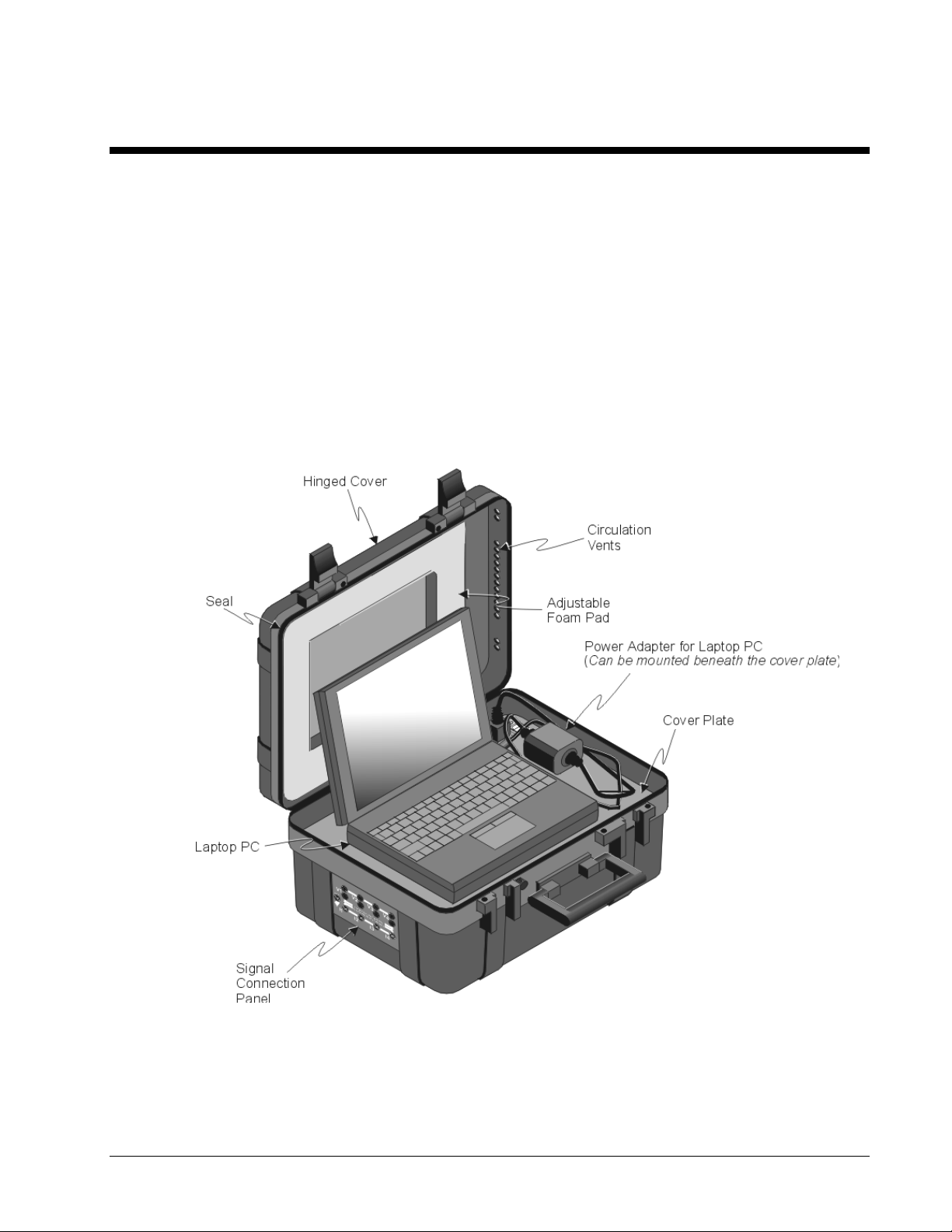
PowerVista/312’s rugged case includes a signal connection panel, AC inlet connection, and cooling fan. A
laptop PC is located on a cover plate, while the data acquisition device is located beneath the plate. An
uninterruptable power supply option is available for the acquisition device. Section 1.2, Understanding the
Hardware, provides more detail.

Figure 1-1. PowerVista/312

PowerVista/312 User’s Manual Introduction and Hardware Setup 1-1

1.1.2 What Is EasyPower Measure ?

EasyPower Measure is a single software application that uses C++ object oriented programming to
accomplish the most critical needs of power system measurement. Each measurement feature represents a piece
of specialty hardware, and in most cases exceeds the scope of that hardware. All features are integrated into a
single fast access database so that any measurement can be retrieved with simple click and drag functionality.

1.1 Understanding the Hardware

Figure 1-1 (previous page) shows the basic hardware arrangement of PowerVista/312. Figure 1-2 provides more
information regarding hardware aspects of the PowerVista/312. Main points from the figure are as follows:

The left side of the case supports the signal connection panel. This panel is where voltage and current signal
inputs are made, as well as a safety ground connection. Various types of connections are illustrated and
discussed in Chapter 4.

The cover plate covers the data acquisition device and the uninterruptable power supply option (if part of your
unit). The laptop’s power adapter can also be mounted beneath the cover plate. A slot at the rear of the plate
permits cable passage. The left side of the cover plate contains circulation vents for forced-air cooling.

The communication cable (or optional WBK20 enhanced parallel port PC-card) links the acquisition device to
the PC via parallel (or enhanced parallel) port.

The 110 VAC outlet (on the cover plate) can be used to supply power to Laptop’s power adapter.

The power switch and LED (on the cover plate). The power switch turns power on or off for the UPS option

and the PowerVista/312 acquisition device. The LED lights when the switch is closed and power is available to
the unit. Note that power to the laptop is not related to the switch or LED.

Dual-lock tabs can be used to secure the Laptop and its power adapter to the cover plate. The dual-lock tabs are
similar to Velcro

A thru-hole (located on the case portion of the latch, just right of the case handle) can be used to attach a seal,
small padlock, or tag, or small chain.

110 VAC power-inlet (on the right side of the unit’s case) connects to a 110 VAC supply via a power cord.
Power through this inlet supplies the data acquisition device, optional uninterruptable power supply (UPS), and
unit receptacles, including the cover plate receptacle (for powering the Laptop).

Fan. The right side of the unit contains a fan for forced-air cooling.

Acquisition Device [Not Shown] – The data acquisition portion of the PowerVista/312 is located beneath the

cover plate and consists of a modified WaveBook. Separate documentation is provided for this portion of the
PowerVista/312.

Uninterruptable Power Supply option (UPS) [Not Shown]. This optional power supply (if ordered) is located
beneath the cover plate. The UPS option provides power to the acquisition device in instances of faltering or no
AC; and can be used as a battery to supply power for up to three hours. Note that the UPS is intended for use by
the acquisition device only. It is not connected to the receptacles that supply power to the laptop PC.

TM

.

1-2 Introduction and Hardware Setup PowerVista/312 User’s Manual

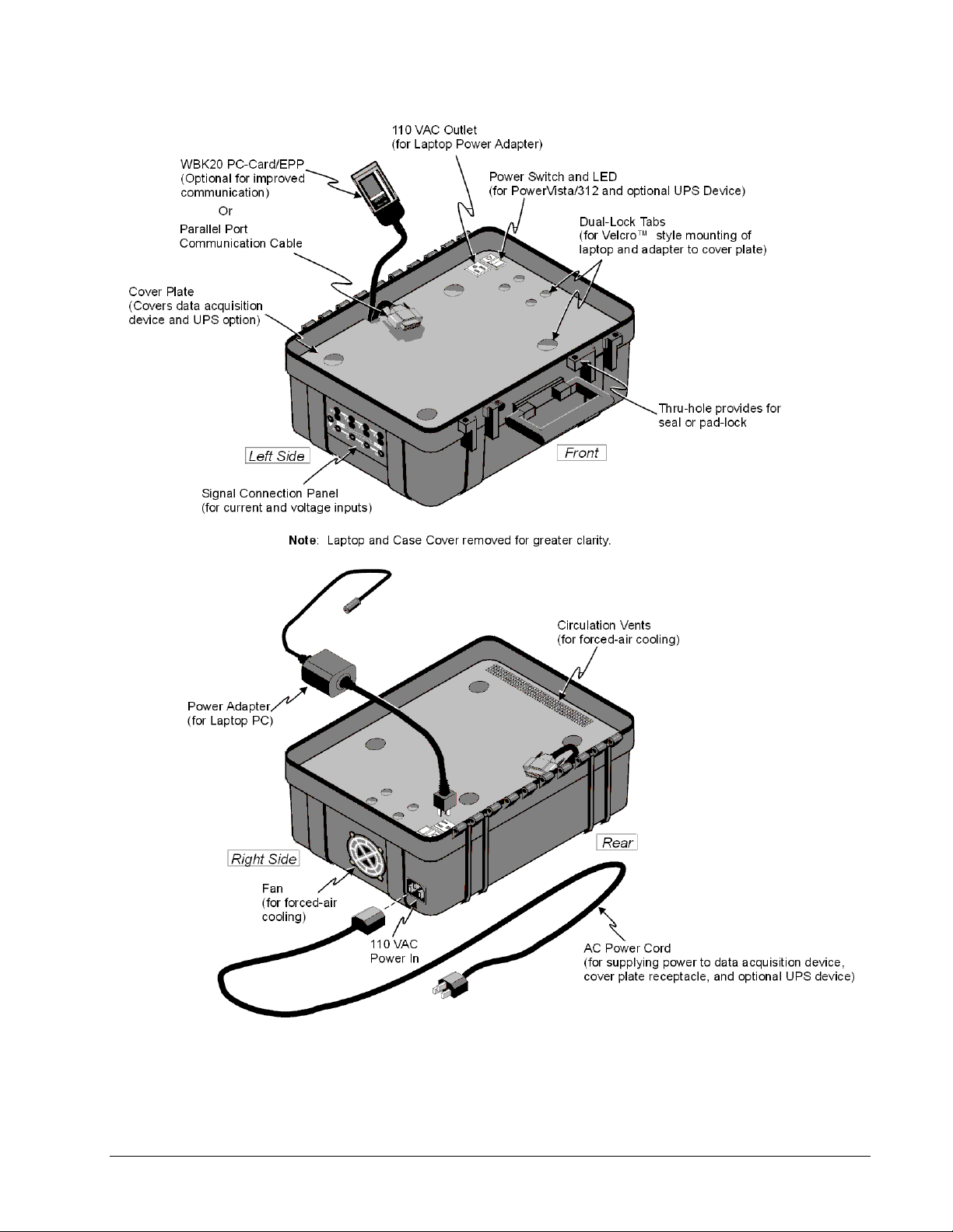
Figure 1-2. PowerVista/312, Hardware Identification

PowerVista/312 User’s Manual Introduction and Hardware Setup 1-3

1.1.3 Frequently Asked Questions

Can I Operate PowerVista/312 with the Unit Closed ?

Yes. As long as your unit is configured for your acquisition, has the signal connections correctly made, and has
been properly powered-up, you can close the unit, lock it, and allow the acquisition to take place automatically.

Note: It is important to keep PowerVista/312’s openings free of obstruction to ensure adequate airflow. Also

see the following question, How Do I Keep the System Cool?

How Do I Keep the System Cool ?

The unit is self-cooled by its own fan, providing the flow-holes for air circulation are not obstructed. The fan
draws air into the right-side of the lower casing. Air flows beneath the cover plate, then up through holes in the
right-side of the plate. When the case cover is closed, air then flows across the laptop and back out through the
flow-holes in right side of the upper casing.

Note: It is important that you keep PowerVista/312’s openings free of obstruction to ensure adequate airflow.

Also keep the fan intake away from dirt and dust to avoid the intake of foreign material.

What Does the UPS Option Do?

The UPS (uninterruptable power supply) is a system option. The UPS is a power distributor and a rechargeable
power source. When fully charged, the UPS option ensures the PowerVista/312 acquisition device will receive
power for up to three hours when there is no AC available, or when there are periods of bad AC. In the first
case the UPS device is functioning simply as a battery.

Note: PowerVista/312’s UPS option is intended only for use with the acquisition device. It is not intended

for use with the laptop and the system receptacles do not have UPS protection.

Where Should I Plug In the Laptop’s Adapter ?

PowerVista/312 contains two 110 VAC outlets that are intended for use by your laptop’s power adapter. If the
power adapter is mounted on the cover plate, you can use the cover plate’s outlet. If you mount the adapter
beneath the cover plate, you can use the internal outlet that is clearly visible near the right side of the device,
once the cover plate is removed.

Note that the system’s 110 VAC power outlets will have power available as long as the PowerVista/312 is
plugged into a live power source. The cover plate switch and LED do not pertain to PowerVista/312’s AC
outlets.

1-4 Introduction and Hardware Setup PowerVista/312 User’s Manual

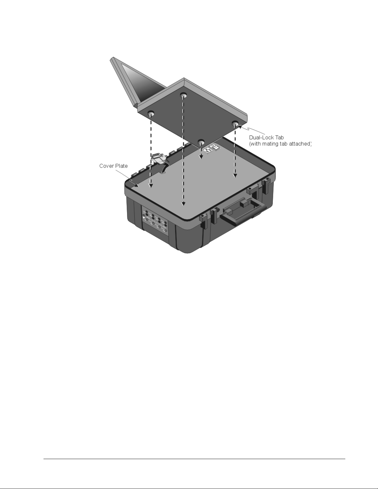
1.1.4 Mounting the Laptop

Figure 1-3. Attaching a Laptop to the Cover Plate

It is a simple task to mount the Laptop to PowerVista/312’s cover plate. When mounting the laptop, remember
to allow room for your laptop’s power adapter; unless you plan to locate the adapter beneath the cover plate as
discussed in section 1.2.3, Connecting the PC). Also, be sure that the laptop will not cover the circulation vents
on the left side of the cover plate.

Mount the laptop as follows:

1. Verify that PowerVista/312’s cover plate and bottom surface of the laptop are clean. This will provide for
optimum adhesion of the dual-lock tabs.

2. Attach a dual-lock tab (with its mating tab still attached) near each corner of the laptop’s bottom surface.
Note that there are two sets of dual-lock tabs. The smaller tabs are for use with the PC’s power adapter.

3. Expose the adhesive of the lower tabs.

4. Carefully place the laptop into position and press firmly.

Note: Use the smaller dual-lock tabs and similar method if you desire to mount the PC’s power adapter to the

cover plate.

PowerVista/312 User’s Manual Introduction and Hardware Setup 1-5

1.1.5 Connecting the PC

This section involves connecting your laptop to the acquisition device via parallel communications cable, and
connecting your laptop to power.

Note: To run the EasyPower Measure program, the following notebook PC requirements are essential:

• Pentium 150 MHz or better.

• At least 32 Mbytes of memory.

• Windows 95 operating system.

• At least a 1 Gigabyte hard drive (data storage).

• 256 kByte or greater disk cache.

• 800x600 display minimum.

• PCMCIA card slot (optional)*

*The PCMCIA card slot is needed if the optional WBK20 PC card will be used for your system. The WBK20
provides enhanced parallel port communications. Refer to WBK20 documentation if applicable to your
application. To connect your laptop computer:

1. Connect your laptop to the data acquisition device using the parallel port connector or the optional WBK20
PC-card. If using the WBK20 option, please refer to the WBK20 documentation received with your card.

2. If you want to locate your PC power adapter beneath the cover plate, complete this step. If not, proceed
with step 3. Remove the cover plate screws and the cover plate. Position the adapter in the normally
hidden compartment and secure with zip ties (tie wraps). Plug the adapter’s AC cord into the lower
compartment 110 VAC receptacle. Position the PC-end of the adapter cord through the cover plate’s cord
grove and remount the cover plate.

3. If you want to locate your PC power adapter on the cover plate, position the adapter on the plate and plug
the AC end of the cord into the plate’s receptacle.

4. Plug the small end of the adapter cable into your laptop’s adapter jack.

Note: For the cover plate receptacle to have power you must first supply power through PowerVista/312’s

110 VAC power in connector (located on the right side of the unit).

1-6 Introduction and Hardware Setup PowerVista/312 User’s Manual

2 Install Software and Change PC Settings

2.1 Introduction to EasyPower Measure Viewer

EasyPower Measure includes two versions of software with its installation. The main version is em.exe and is
the full-featured version of EasyPower Measure. This version is supplied to you under the legal software
licensing agreement, and cannot be supplied to any other third party. A second version, emview.exe, is a
viewer only version that has all measurement functions disabled. The viewer version is also a "read only"
version of EasyPower Measure. Thus, it can be included on CD ROM as a browser for a well organized archive
backup of collected data. The viewer version may be freely distributed to any third party along with any
EasyPower Measure database files. Make sure that all files in the viewer directory are included with any
archive or transmittal of data, or the viewer will not function.

With the use of EasyPower Measure software, PowerVista/312 measurement capabilities include:

• Phasor Diagram.

• Detailed Harmonics.

• Spectrum Analyzer.

• Cycle-by-Cycle Capture.

• Event Capture with Demand Recording.

Each of these features has a complete section dedicated to their use and proper application.

2.2 Install EasyPower Measure

Complete the following steps to install EasyPower Measure onto your laptop PC. At the time of installation, all
files necessary to run the program will be installed.
Once the software has been installed, several modifications must be made to the PC to allow real-time capturing
and recording of data. These setting modifications are absolutely necessary, and without these you can expect
significant interruptions during data collection. The required changes, such as disabling power management, are
sections 2.3 through 2.7.

Note: Early in the installation process you will need to enter your product’s serial. The serial number consists

of eight digits preceded by the letters EPM.

1. Power up your laptop.

2. Insert Disk1 and follow the Installation Wizard on-screen prompts.

3. Make required changes to PC settings as described in sections 2.3 through 2.7.

2.3 Disable Power Management

The power management features of notebook PCs are the culprits for the majority of their lost performance.
Unfortunately, turning off the feature is most often a two step operation. All power management features of the
notebook PC must be disabled. This will keep vital equipment from timing out (hard drive, PC card, display)
and will allow the processor to run at rated speed.

• System BIOS: The first location to turn off power management features is within the system BIOS. To

modify the settings there, during boot up of the machine, press the function key noted in the display to access
BIOS settings (typically F1 or F2). Find the power management section and disable all of the power
management features.

• Control Panel: The second location to turn off power management is within Windows 95 itself. To modify

settings within Win95, access the system Control Panel, and start up the Power icon.

PowerVista/312 User’s Manual Install Software and Change PC Settings 2-1

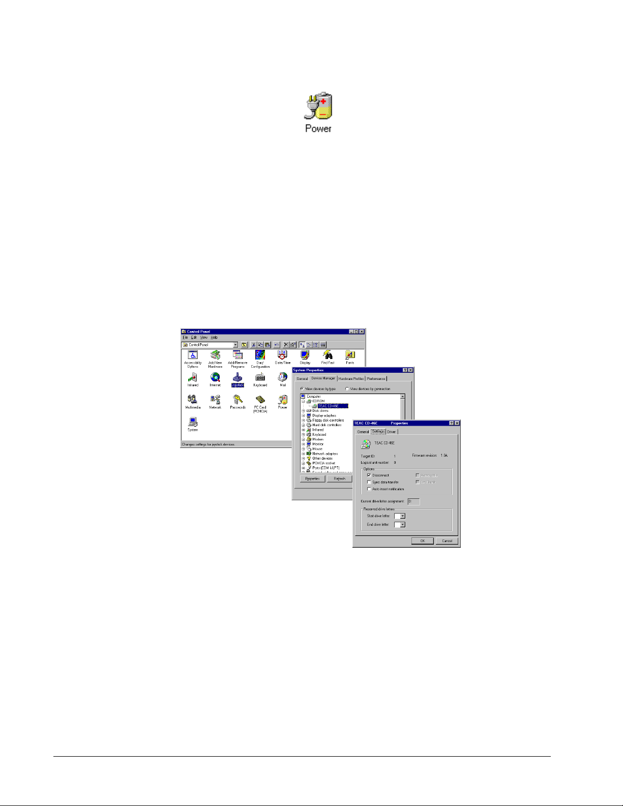
Figure 2-1. The Control Panel Power Management ICON.

Once activated, go through each of the tabbed folders and disable all power management features. In most cases
this includes: Power, Disk Drives, and PC-Cards. Make sure that none of these have power management options
checked and operational. You will have to re-boot your machine to make these changes take effect.

2.4 Disable CD ROM Auto Insert Notification

One of the unseen and often overlooked process time stealers is the Auto Insert Notification for CD ROMS.
This feature auto starts a CD ROM software installation as soon as a CD ROM is inserted in the drive. In the
Control Panel, under System icon, then Device Manager tab, the CD ROM device is located among a list of all
equipment presently allocated for the PC. The Auto Insert Notification selection is located under the CDROM
device, then installed model, then device Settings Tab. This selection should be unchecked to keep Win95 from
taking process time by auto-polling the CD ROM to see if an installation disk has been loaded.

Figure 2-2. CD ROM Auto Insert Notification.

2.5 Disable Win95 Screen Savers and Energy Management Functions

Screen savers and energy management functions are additional process time stealers. These functions also need
to be completely disabled to be able to run EasyPower Measure as a real time un-interrupted application. The
energy management functions are also the most customized setup configuration for the PC, where vendors apply
all types of specialty functions as well as non-standard Win95 interfaces. With such variations, suffice it to say,
any energy management function or screen saver utility (Win95 or other installed program) must be disabled.

2-2 Install Software and Change PC Settings PowerVista/312 User’s Manual

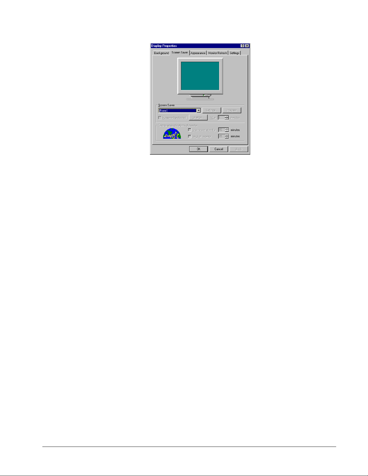
Figure 2-6. Default Screen Saver and Energy Management in Win95.

2.6 Disable Virtual Memory Management [if necessary]

The virtual memory settings within Win95 are almost always defaulted such that Windows is managing your
virtual memory. There really is no real problem with this, and there are added benefits such as an increased
virtual disk cache (using PC memory). This increases performance when writing events to disk so that there is
(for burst type events) no waiting on the hard drive to write events. Event throughput thus in this mode is not
limited by the write speed of the drive. In most systems, there is adequate drive throughput to continuously
capture events with no loss of data for 50 and 60 Hz systems.
If your particular system however is running into the Windows background processing dilemma, there is a
solution. On occasion, Windows will decide to clean up its virtual memory on disk and unload a few dynamic
link libraries. When this happens, process time is taken away from the application.

This has not seemed to be an issue with Version 1.0 of EasyPower Measure, but if it is a problem there is
clearly one simple solution. Disable virtual memory management. This will require the PC to have at least
32 M of system RAM so that the operating system and EasyPower Measure can reside together. This has been
used successfully to run the application within such a dedicated environment for real-time data acquisition.
When the user desires to review measurements and also use other Windows applications, it is recommended that
virtual memory management be re-instated. For any changes in virtual memory management, the system will
have to be re-booted.

PowerVista/312 User’s Manual Install Software and Change PC Settings 2-3

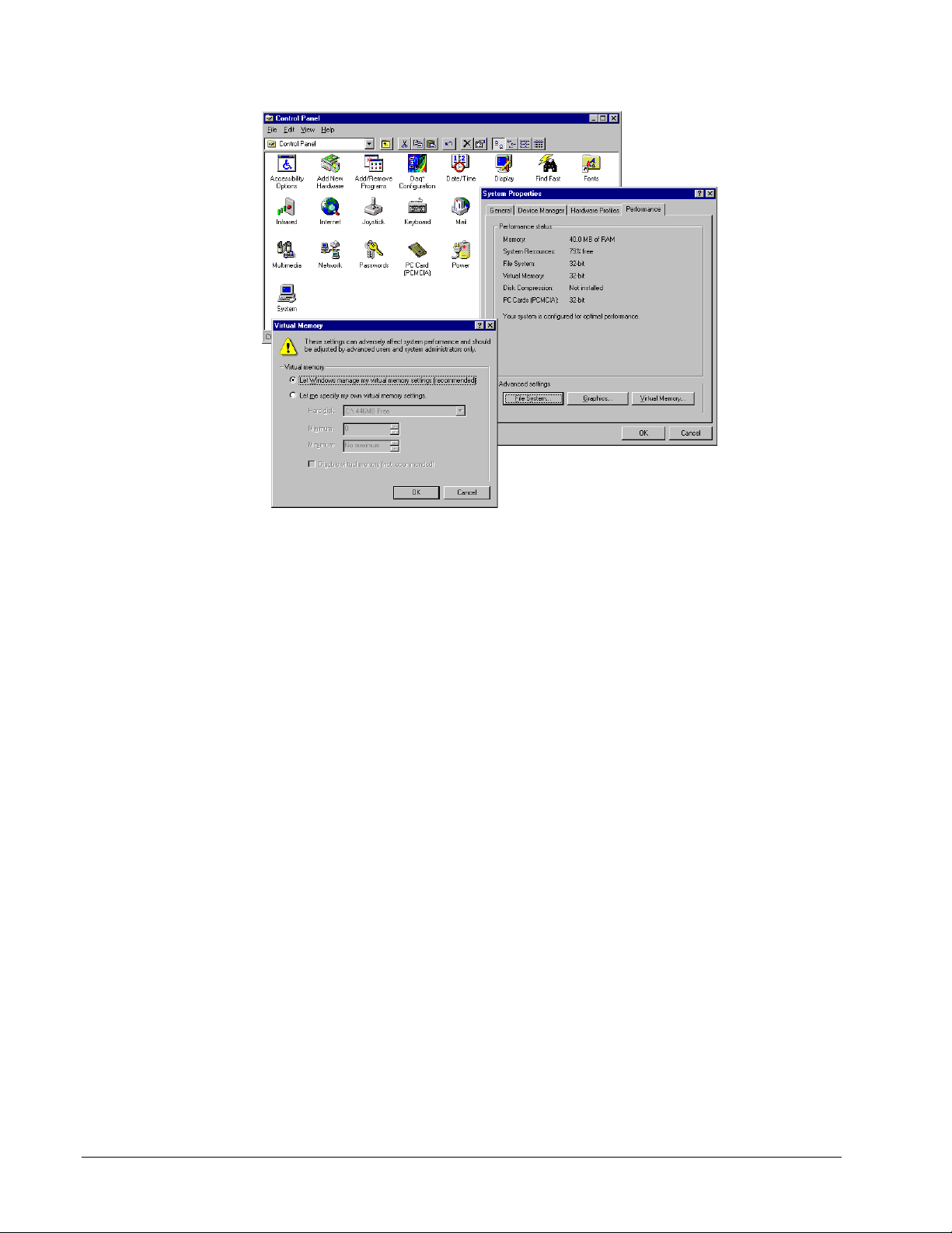
Figure 2-4. Virtual Memory Management.

2.7 Disable Additional Process Time Stealers [if necessary]

A few other process time stealers that may have to be disabled include:

• Auto EMail Answer.

• Any background Network Communication.

• Sounds (with this enabled, Windows will load and play a wave file for system responses).

• Auto Answer Modems.

2-4 Install Software and Change PC Settings PowerVista/312 User’s Manual

3 Software Framework

3.1 Overview

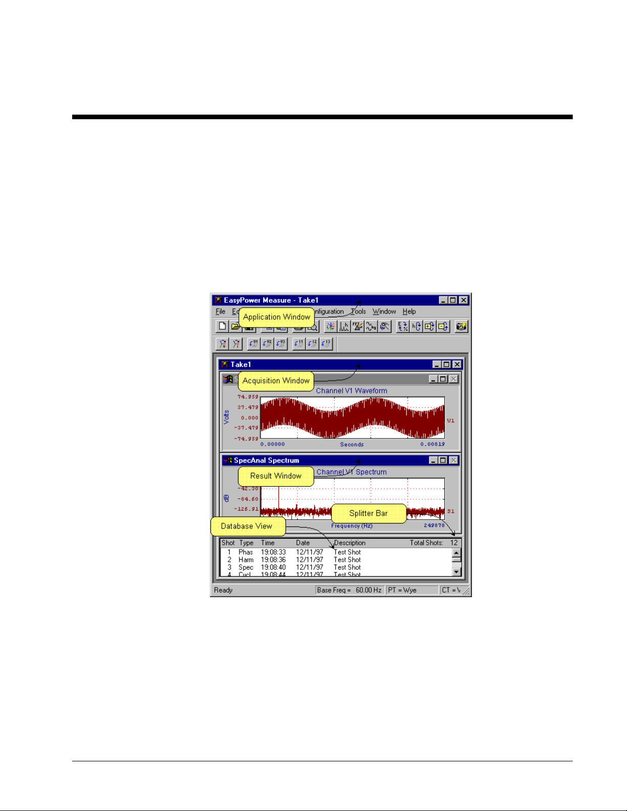
EasyPower Measure is a Windows multiple document interface (MDI) application. The software uses the same
style of interface seen in typical Windows applications such as Microsoft Word or Excel. The application runs
within an MDI frame window that has a menu bar and tool bar attached to the top. Upon initiating EasyPower
Measure, it automatically maximizes itself so that it fills the entire screen of your PC. You are free to resize the
Application Window, but will find that on 800x600 displays, a maximized screen is best to capture and view
data.

Within the Application Window are Acquisition Windows. Each of the Acquisition Windows contains several
Result Windows that display measurement results, and an integrated Database View in the lower pane. A
splitter bar (moved to view more or less of the database shot list) separates the Result Windows from the
Database View. A sample EasyPower Measure interface screen is shown in Figure 3-1.

Figure 3-1. EasyPower Measure MDI Interface.

When you start EasyPower Measure for the first time, there will be only one Acquisition Window, and its Result
Windows will be set for Phasor Diagram measurements.

PowerVista/312 User’s Manual Software Framework 3-1

3.2 File Access

File access for EasyPower Measure follows standard Windows convention for a multiple document interface
(MDI) application with only one significant exception. Since data collection is considered mission critical, and
loss of data is to be avoided at all costs, once a database has been saved with a supplied name using File Save
As, no additional saving is necessary.

With this method, if collected data appears in the shot list, then it has already been written to the database file on
disk. This is true even if additional data captures have been snapped into the database. When terminating the
application or an acquisition window under this condition, the user will not be prompted to save a database file.
Thus, if the database file is in tact and not corrupted, then data has been archived successfully.

3.2.1 File New

File New opens a new Acquisition Window with an associated EasyPower Measure database file assuming
default parameters for all configuration settings. The user can now collect data into this temporary database. To
save collected data permanently on the hard drive, the user must save the database using File Save As. It is
recommended that as soon as a new database is created with File New that the database be saved. If Win95
were to crash with a temporary file in use, the data collected in that temporary file will be lost. If the database
has already been saved and named, then collected data will always be written directly to the database file on
disk. No additional saving is necessary, and the user is not prompted to save when terminating the application
or an Acquisition Window.

3.2.2 File Open

File Open opens an existing database file and associates it with an Acquisition Window. Collected shots will be
displayed in the Database View. All data collected from this point will be appended to the opened file.

3.2.3 File Save As

File Save As is used to supply a registered disk file name to the database associated with the presently selected
Acquisition Window. When using File New, File Save As should be executed next. Without this action,
captured data is snapped and stored into temporary files. Upon exiting the application or Acquisition Window,
the user will be prompted to supply a registered disk file name through the File Save As dialog window.

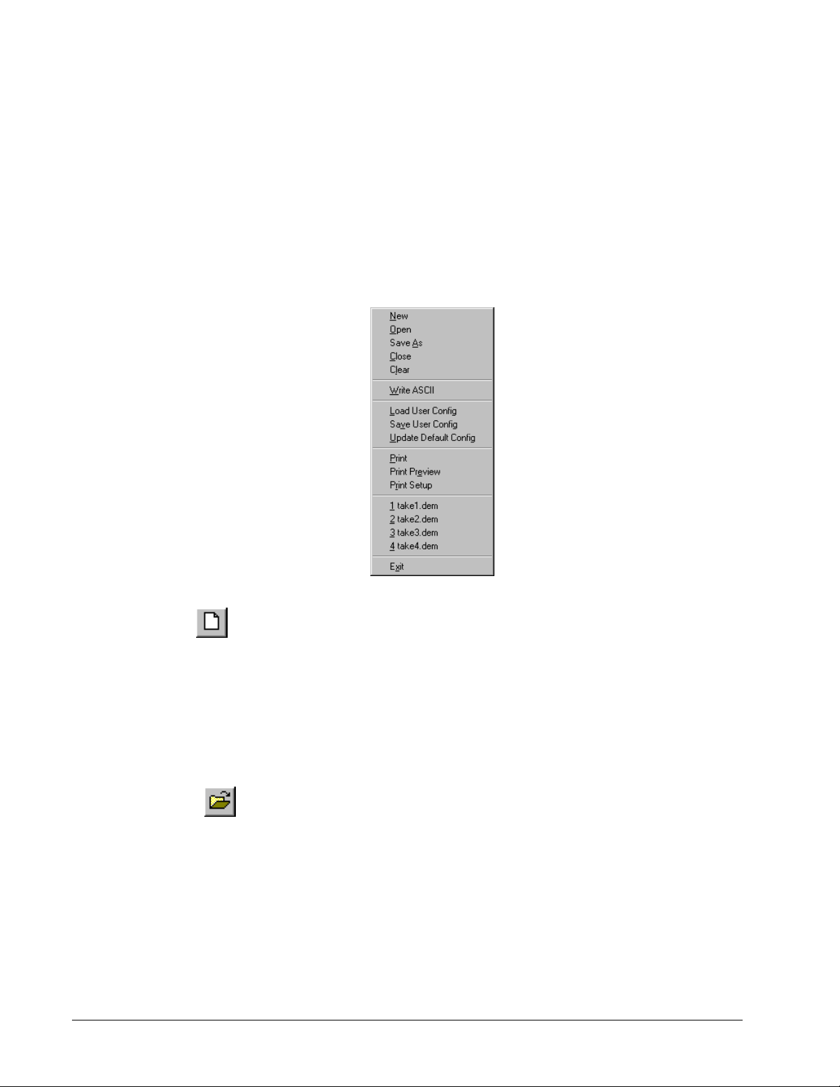
Figure 3-2. File pull down menu.

3-2 Software Framework PowerVista/312 User’s Manual

3.2.4 File Close

File Close terminates the presently selected Acquisition Widow. This is similar to a left mouse click on in
the upper right corner of the Acquisition Window. If shots have been saved in a temporary database file, the
user will be prompted automatically to save the captured data with a registered file name.

3.2.5 File Clear

File Clear deletes all shots from the presently viewed database. The user is prompted with:

Delete all entries in database?

before the database is cleared. Clicking on OK will destroy all captured shots and is non-recoverable. Care
should be taken before clearing all shots from a database.

3.2.6 Write ASCII

Write ASCII outputs ASCII text files of collected digitized data, the shot list, and the system setup. The data
output is determined by which measurement feature is presently selected (has focus). The user is prompted for
an output filename. EasyPower Measure will automatically choose filename extensions for the data being
saved. For some Result Windows, more than one text file could be written to disk. Table 2 lists the filename
extensions used with each measurement feature.

Measurement Feature Extensions Comment

Phasor Diagram .phs All data in one file.

Detailed Harmonics .hrm .hra .hrw Magnitudes, angles, waveshapes respectively

Spectrum Analyzer .spm .spw Magnitudes and waveshapes respectively

Cycle-by-Cycle Capture .cyc All data in one file

Event Capture .evt All data in one file

Demand Logging .dm1 to .dm8 In order of demand shots in database.

Harmonics Logging .dh1 to .dh9 In order of demand harmonic shots in database.

System Setup .stp All critical configuration information.

Shot List .sht All items listed in shot list.

Table 2. ASCII filename extensions.

3.2.7 File Exit

File Exit terminates the application. If any Acquisition Windows need to be saved, the user will be prompted.
The default configuration file is also updated. This is similar to a left mouse click on
corner of the Application Window.

3.3 User Configuration

The complete configuration of each Acquisition Window in the application workspace can be saved as a user
configuration to disk. This configuration file allows the user to set up a customized data collection work space
and save it for later use. With simple file loading, each previously saved user configuration can be loaded to
minimize instrumentation setup time and create a consistent measurement procedure. In addition to the user
configuration, EasyPower Measure will always remember the configuration setup when the application was last
terminated. Configuration files store the complete application configuration including:

• All configuration parameters for each Application Window as seen in the configuration dialogs.

• All Acquisition Window sizes and positions.

• Up to eight (8) acquisition windows.

•

Result Window size and position.

A directory of typical user configurations has been supplied with this program. Table 3 below lists the
configuration file names and notes particular applications.

in the upper right

PowerVista/312 User’s Manual Software Framework 3-3

Table 3. Supplied User Configuration Files.

Configuration File Comment

120VdemY.cfg 120 V, Wye connected PTs, gains set for maximum demand accuracy.

120VevtY.cfg 120 V, Wye connected PTs, gains set for event capture.

208VdemD.cfg 208 V, Delta connected PTs, gains set for maximum demand accuracy.

208VevtD.cfg 208 V, Delta connected PTs, gains set for event capture.

277VdemY.cfg 277 V, Wye connected PTs, gains set for maximum demand accuracy.

277VevtY.cfg 277 V, Wye connected PTs, gains set for event capture.

480VdemD.cfg 480 V, Delta connected PTs, gains set for maximum demand accuracy.

480VevtD.cfg 480 V, Delta connected PTs, gains set for event capture.

3.3.1 Load User Config

Load User Config allows the user to load previously stored configuration files. This command prompts the user
to: “Close all acquisition windows?” since it will close all presently opened Acquisition Windows and load a
completely new setup. If OK is selected and if there were any Acquisition Windows using temp files to save
shots, the user will be prompted to save each previously unsaved database.

Note: A loaded User Configuration does not reload any associated databases. The User Configuration is a

template of the entire configuration without collected data. Once the User Configuration is loaded, the
File Save As command should be used to save any collected shots as well as to make that database able
to permanently archive automatically.

3.3.2 Save User Config

Save User Config saves the user configuration to disk in a selected or entered filename and directory location.

Note: A saved User Configuration will not contain the filenames for any associated databases presently

displayed in the application. The User Configuration saves a template of the entire configuration
without collected data. Once the User Configuration is reloaded, the File Save As command should be
used to save any collected shots as well as to make that database able to archive permanently
automatically.

3.3.3 Update Default Config

The default configuration is saved to the disk file default.cfg during the closing procedure of the application.
However, if the user wishes to update the default configuration file at any time, this command may be invoked to
do so. The default configuration file is stored in the EasyPower Measure installation directory.

Program Failure: If EasyPower Measure does not load properly, or if it appears to have extreme erratic
behavior, there is the possibility that the default configuration file has been corrupted. This file can be deleted at
any time and it will not harm operation of the program. Any settings previously saved in the file will of course
be lost, and the user will have to redefine the system configuration. User Configurations however can be loaded,
assuming they have integrity and have not been corrupted.

3.4 Printing

Printing of result windows for each acquisition measurement feature can be accomplished through Windows
standard file printing. Printing is performed in two possible ways, which is governed by the Print Summary
Pages setting in the Configuration / Preferences dialog. If this setting is checked, summary printouts for result
windows are accumulated into one or more condensed reports. If this setting is not checked, then a single
graphic is printed for the presently selected result window.

3-4 Software Framework PowerVista/312 User’s Manual

3.4.1 Print

Print either a result summary or a single result window to the output device selected in Print Setup. The result
summary option is selected in the Configuration / Preferences dialog.

Note: This command operates on the Result Window with focus.

3.4.2 Print Preview

Perform a Print Preview to screen of either a Result Summary or a single Result Window as it would appear on
the output device selected in Print Setup. The Result Summary option is selected in the
Configuration/Preferences dialog. If no printer has been installed via Win95 standard print device selection,
then Print Preview will not function. To run Print Preview, a printer must be installed even if printing will never
be performed from the measurement PC.

Note: This command operates on the Result Window with focus if Result Summaries are not selected.

3.4.3 Print Setup

Print Setup selects the printer for Print and Print Preview, and specifies Windows standard parameters for
printing on an output device.

3.5 Copy - Paste Shots

The copy and paste shots feature built into EasyPower Measure makes the application a flexible data gathering
and organizing tool. Copy Shots and Paste Shots is supplied to copy shots from one database to another, thus
allowing the user to construct databases with only desired measurements.

The EasyPower Measure database has been designed for speed, and thus contains two files for each database.
The first file with extension .dem is the main data holding file. The second file is the pointer file with a .kem
extension. The pointer file contains pointers for fast random access reads of the main data file, and the
description seen in the database view for each shot. The size of the .dem file will always be much larger than its
companion file since it holds the actual snapped data.

Note: Both the .dem and .kem files are essential to define a database. If either one of the pair is deleted,

renamed or modified, then access to the database is impossible.

The database has been designed for speed writing during event capture. For this reason, the database files
cannot have individual shots deleted from within the database. The entire contents of the file can be removed
(see File / Clear) however this is no help in saving only a small portion of data out of a large file. To solve this
problem, shot copy and paste between Acquisition Windows (and thus respective databases) was integrated into
the application.

3.5.1 Copy Shots

Contrary to its command name, Copy Shots does not actually copy data, but retains a list of desired shots that
the user wants to transfer to an alternate database.

The user utilizes the Database View multiple selection list box feature (similar to the file lists in Win95
Explorer) to select shots in an Acquisition Window. Once the shots are selected (highlighted), the user should
issue the Copy Shots command. This command copies the selected list of shots and the source of the shots to
memory for future access.

After selecting (gaining focus by a left click on title bar) the paste acquisition window for the copied shots, the
Paste Shots command should be issued.

Note: There is a 5000 shot maximum limit on the number of shots that can be copied at one time.

PowerVista/312 User’s Manual Software Framework 3-5

3.5.2 Paste Shots

The Paste Shots command accesses the list of shots to copy stored in memory (put in memory by Copy Shots).
This list also contains the desired source database. Paste Shots performs all of the read and write commands
necessary to transfer a copy of the shots to the newly selected Acquisition Window. As each shot is read into
memory, the source Acquisition Window can be seen drawing each shot. This is an update monitor as well a
visual verification of the shots copied.

Note: There is a 5000 shot maximum limit on the number of shots that can be copied at one time.

3.5.3 Change Shot Titles

The Change Shot Titles command allows the user to edit and modify the site description and shot description
titles. Once data has been collected in the field, invariably, documentation changes and adjustments will be
necessary to properly describe the collected data. These are the only modifications that can be made to
previously collected data. To maintain the integrity of the data, and the parameters under which it was collected,
no other items in the Critical Configuration can be modified for an archived shot. Title changes have been
allowed here to facilitate proper documentation and editorial enhancements.

3.6 Copy to Clipboard

The copy to clipboard features within EasyPower Measure give the user graphical, text and delimited text
access to all results reported within any Result Window. Graphics are copied as Windows metafiles and
bitmaps, text is copied as straight non-proportional font column oriented results, and delimited data is copied
with tab delimiters for direct porting into spreadsheets. The delimited data feature gives users click and paste
access to all digitized data captured within the application for post processing.

3.6.1 Copy Graphics or Text

Copy Graphics or Text is used to copy report quality output onto the system clipboard. Graphics are copied in
both a Windows metafile format as well as a bitmap format. Text is copied as non-proportional spaced, column
oriented report. Both graphics and text reports will match the data presented identically in the result view
copied.

Note: This command operates on the Result Window with focus.

The text report may have to be slightly modified once pasted into the document that is presently being edited.
Typically, users will be creating a document with a proportional spaced font. Proportional spaced fonts cannot
be used to align space oriented columns (the technique used in the EasyPower Measure reports). It is suggested
that the pasted report text be modified to incorporate the Courier or Courier New font. Both are non­proportionally spaced fonts.

Once a graphic metafile has been pasted into a document, it may be scaled (click and drag on corners) to fit the
page according to the users taste. The metafile may also be edited. Editing of a metafile in a word processor
should be tested, as these editors have been known to effect permanent undesired modifications to the graphic
content without any user modifications.

3.6.2 Copy Delimited Data

Copy Delimited Data allows the user to have full access to actual digitized and calculated values. This function
copies the internally held data to the system clipboard for paste within any Windows application that offers
clipboard paste functionality. In most cases, this data will be imported into a spreadsheet for post processing.
Delimited data copying is supplied for both the graphic result windows as well as the tabulated text result
windows.

Note: This command operates on the Result Window with focus.

3-6 Software Framework PowerVista/312 User’s Manual

3.7 Tools

Several tools have been supplied to make accessing results simple and convenient. With a single click of these
toolbar buttons the user can access all recorded data quickly with several view formats so that measurements can
be assessed and verified before continuing additional collection.

3.7.1 Engineering vs. Percent Toggle

Engineering vs. Percent toggles harmonic results from percent on fundamental base to physical units, i.e. volts
and amps. This will apply to the Phasor Diagram and the Detailed Harmonics in both their tabulated and
graphical results. These two acquisition features have separate selections in their configuration for toggling this
option, but the toolbar will modify the setting appropriate to the measurement feature in view.

3.7.2 Cycle Graph Forward

Cycle Graph Forward causes the graphical and tabulated text results to be scrolled to the next view choice. In
each acquisition configuration dialog there are display choices for what collected data item is to be displayed
(via drop down lists). This method of displaying data has been adopted since:

•

it is impossible to display all of the data collected for a given acquisition.

• there is a need to see the acquired data.

• collected data falls within an acquisition type.

There are three methods for moving to a particular data display,

1. Access the acquisition configuration dialog (for example, Configuration / Phasor Diagram), and

select a display choice.

2. Press the

Cycle Graph Forward

button to select the next data item(s) to display as ordered in the drop

down list choices in each acquisition configuration dialog.

3. Press the Cycle Graph Backward button to select the previous data item(s) to display as ordered in the

drop down list choices in each acquisition configuration dialog.

When Cycle Graph Forward has reached the end of the display list, it cycles to the top of the list in a circular
fashion. Likewise, when Cycle Graph Backward has reached the beginning of the display list, it cycles to the
bottom of the list in a circular fashion. Thus, all data views can be displayed very quickly using repeated clicks
on the Cycle Graph Forward and Cycle Graph Backward buttons. Table 4 lists the acquisition views and how
they are affected by Cycle Graph Forward and Cycle Graph Backward.

Table 4. Cycle Graph Forward and Backward Effects.

Acquisition Type Effect

Phasor Diagram Cycles Phasor Graphics and Phasor Demand result windows.

Detailed Harmonics Cycles all result windows.

Spectrum Analyzer Toggles from dB to Linear.

Cycle by Cycle Cycles all result widows.

Event Capture Cycles all result windows.

Demand Logging Not cycled.

Demand Harmonic Logging Not cycled.

PowerVista/312 User’s Manual Software Framework 3-7

3.7.3 Cycle Graph Backward

Cycle Graph Backward causes the graphical and tabulated text results to be scrolled to the previous view choice.
In each acquisition configuration dialog there are display choices for what collected data item is to be displayed
(via drop down lists). This method of displaying data has been adopted since:

•

it is impossible to display all of the data collected for a given acquisition.

• there is a need to see the acquired data.

• collected data falls within an acquisition type.

There are three methods for moving to a particular data display,

1. Access the acquisition configuration dialog (for example, Configuration / Phasor Diagram), and

select a display choice.

2. Press the Cycle Graph Forward button to select the next data item(s) to display as ordered in the drop

down list choices in each acquisition configuration dialog.

3. Press the

drop down list choices in each acquisition configuration dialog.

When Cycle Graph Forward has reached the end of the display list, it cycles to the top of the list in a circular
fashion. Likewise, when Cycle Graph Backward has reached the beginning of the display list, it cycles to the
bottom of the list in a circular fashion. Thus, all data views can be displayed very quickly using repeated clicks
on the Cycle Graph Forward and Cycle Graph Backward buttons.

Table 4 (see Cycle Graph Forward) lists the acquisition views and how they are affected by Cycle Graph
Forward and Cycle Graph Backward.

Cycle Graph Backward

3.7.4 Cycle Harmonics Forward

Cycle Harmonics Forward causes the harmonics tabulation in the Phasor Diagram to be scrolled to the next view
choice. The harmonics tabulated data view can also be selected through the Configuration / Phasor Diagram
dialog, Harmonics View list box. When Cycle Harmonics Forward has reached the end of the display list, it
cycles to the top of the list in a circular fashion.

3.7.5 Cycle Harmonics Backward

Cycle Harmonics Backward causes the harmonics tabulation in the Phasor Diagram to be scrolled to the next
previous choice. The harmonics tabulated data view can also be selected through the Configuration / Phasor
Diagram dialog, Harmonics View list box. When Cycle Harmonics Backward has reached the top of the display
list, it cycles to the end of the list in a circular fashion.

button to select the previous data item(s) to display as ordered in the

3.7.6 Take Snapshot

Take Snapshot will copy the acquisition data presently in view to the integrated database, appending it to the
end. If the database file was opened from a previous session using File Open, or if after File New it has already
been saved using File Save As, then data will be saved directly to the file on the hard disk and archived
permanently. If the present acquisition is a new window and has not been previously saved, results are stored in
a temporary hard disk file (transparent from the user) until saved via the File Save As command.

Take Snapshot will take database shots for all but one acquisition feature and two database entry types. Table 5
lists each shot type with its four letter pneumonic as seen in the Database View.

3-8 Software Framework PowerVista/312 User’s Manual

Table 5. Shot Four Letter Pneumonics for Database View.

Shot Type Shot Type Pneumonic

Phasor Diagram Phas

Detailed Harmonics Harm

Spectrum Analyzer Spec

Cycle-by-Cycle Cycl

Event Capture Evnt - Not Snapped

Demand Logging Demd - Not Snapped

Demand Harmonics
Logging

Demd - Not Snapped

3.8 Window Management

EasyPower Measure is a multiple document interface (MDI) application. This means that movement and
resizing of any windows follows standard Windows graphical user interface conventions. EasyPower Measure
has been developed under the Microsoft C++ SDK and uses C++ object oriented coding for all window
management.

3.8.1 Determining Focus

As with any MDI application, Focus determines what window is selected so that the application can respond
appropriately to a users commands. The title bar for each Result Window will highlight in the system focus
color (which can be configured via Display under the Win 95 Control Panel) when any part of the window is
selected.

Also, the Database View can achieve focus by clicking within its top column label area. Database View focus
will not activate a highlighted title bar (there is no title bar to conserve space), but will display the
binoculars within its top column label area.

focusing

Once a window has focus, commands like

Copy Graphics or Text

will perform their action on the window that has focus.

Clicking on the title and border of any window will give that window focus. But in addition to giving focus, the
same mouse actions can be used to:

• Move the window: The title bar of each window can be grabbed (left mouse click and hold) while

repositioning it to another location within its parent window.

• Resize the window: Moving the mouse over the borders of any window will change the mouse cursor

to a symbol for resizing the window from top, bottom, sides, or corners. With the mouse cursor in its
modified state, left mouse click and hold to resize the window within the parent window.

The Parent-Child relationship of windows within EasyPower Measure is as follows:

Parent Child

Win95 EasyPower Measure Application Window
Application Window Acquisition Windows
Acquisition Window Result W indows, Database View

PowerVista/312 User’s Manual Software Framework 3-9

3.8.2 Cascade

Cascade will auto-arrange all Acquisition Windows in a folder arrangement where windows are overlaid with
title bars showing.

3.8.3 Tile Horizontal

Figure 3-3. Acquisition Windows Cascaded.

Tile Horizontal will auto-arrange all Acquisition Windows so that each is seen fully and all occupy the entire
visible application space. Acquisition Windows share the space in a horizontal mode where the vertical
dimension is divided evenly between each window.

3.8.4 Tile Vertical

Tile Vertical will auto-arrange all Acquisition Windows so that each is seen fully and all occupy the entire
visible application space. Acquisition Windows share the space in a vertical mode where the horizontal
dimension is divided evenly between each window.

Figure 3-4. Acquisition Windows Tiled Horizontally.

3-10 Software Framework PowerVista/312 User’s Manual

Figure 3-5. Acquisition Windows Tiled Vertically.

3.8.5 Arrange Icons

If any of the Application Windows have been minimized, Arrange Icons will reposition and line up the
minimized windows at the lower left corner of the application space.

3.8.6 Autosize Result Windows

Autosize Result Windows uses a default window arrangement to determine Result Window locations so that the
maximum amount of measurement data is visible. When this is enabled, any resizing of the application view
space will result in an automatic resizing of all Result Windows. If this feature has been disabled (via the
Window / Auto Size Result Windows menu item) the Result Windows can be moved and sized to meet the
specific view needs of a user. Once re-enabled, Result Windows will automatically snap back into place and
user modifications will be lost.

Note: The most common method of automatically resizing Result Windows is by moving the Splitter Bar that
separates the Result View area from the Database View area.

3.9 Toolbar and Status Bar Visibility

The toolbars and status bar are used to give the user quicker access to vital functions and information while
measurement taking. Each can be shown or hidden based upon the status selected within the View menu. The
present status and location of each toolbar will be remembered next time the application is run.

The toolbars are docking enabled, which means that they can either float at any location within the application
workspace, or can be docked to any of the four sides of the application workspace. This gives the user full
Win95 toolbar functionality, and a customized location similar to the Win95 startup menu bar.

The status bar always remains at the bottom of the Application Window. It is updated on a regular basis
depending upon the present acquisition being performed.

PowerVista/312 User’s Manual Software Framework 3-11

3.9.1 Main Toolbar

As of Version 1.0, the Main Toolbar incorporates the following direct access functionality:

File New Cycle-by-Cycle

File Open Event Capture

Copy Graphics or Text Toggle Engineering vs. Percent

Copy Delimited Data Cycle Harm Tabulation Forward

Copy Shot Cycle Harm Tabulation Backward

Paste Shot Cycle Graph Forward

Print Cycle Graph Backward

Print Preview Take Snapshot

Phasor Diagram Input Level Meter

Detailed Harmonics Context Sensitive Help

Spectrum Analyzer

Each of the toolbar buttons is discussed in else where in this manual.

3.9.2 Phasing Toolbar

As of Version 1.0 the Phasing Toolbar incorporates the following direct access functionality:

Cycle Voltage Phasing Invert V3

Cycle Current Phasing Invert I1

Invert V1 Invert I2

Invert V2 Invert I3

The Phasing Toolbar is used to correctly phase input voltages and currents so that proper watts and vars are
calculated on a three phase basis. By viewing the Phasor Diagram, the voltage leads and current transducers can
be connected one time, and then have phase rotation and CT inversion corrections performed via software. In
this way, exposure is limited when making dangerous connections in tight locations where the system voltage
level exceeds 120/208 volts.

3-12 Software Framework PowerVista/312 User’s Manual

Each of the toolbar buttons can also be set in the Configuration / System dialog.

See the Phasing Application note in Phasor Diagram Application.

3.9.3 Status Bar

The Status Bar is used to display detailed tool tips and measurement status on the left, as well as several
important configuration items that give a quick glance reaffirmation of settings.

Figure 3-6. Status Bar.

Items in the Status Bar include:

• Application Status: is on the far left, and alerts the user to the present condition of the program. It will show one

of the following messages:

⇒ Ready The program is ready for input.

⇒

Capturing Data The program is presently capturing data.

⇒ (Tool Tip Info) A slightly longer description for toolbar buttons.

• Base Freq: is the base frequency as set in the Configuration / System dialog.

• PT: is the PT Connection item as set in the Configuration / System dialog.

• CT: is not presently used. In a future revision of

EasyPower Measure

, CT winding connections will be

incorporated.

• FIFO: displays the number of FIFO (first-in-first-out) buffer overruns the hardware has experienced since data

acquisition was initiated. This number should be zero in all cases where the notebook PC processing power and
system configuration settings allow all computations and display to be completed without loss of data.

Note: This status item is the one indication available to alert the user of either an under-powered

notebook PC or configuration settings that are unreasonable (asking for too much data
collection and display too fast).

EasyPower Measure has been designed to recover from any FIFO buffer overrun. This means that data
collection will continue, but data has been lost or missed. This gives the user flexibility to use under-powered
notebooks and still gather meaningful information for non-continuous acquiring functions, i.e. Phasor Diagram,
Detailed Harmonics, and Spectrum Analyzer. Continuous functions (Cycle-by-Cycle and Event/Demand
Capture) on the other hand will misrepresent collected data if a FIFO overrun has occurred. Details for the three
continuous functions are described below.

⇒

Phasor Diagram FIFO Overruns: will show when the system is being taxed, however in the most part can
be ignored since real-time collection of data is not occurring. Each cycle displayed on the phasor diagram
will be correct, even with significant FIFO overruns. The phasor diagram performs all demand calculations,
a complete harmonic decomposition to the 50

th

harmonic on all signals, and updates the display as often as

the Update Rate specifies in the Configuration / Phasor Diagram. At a 0.1sec (10 times per second)
update rate, to perform all of these calculations at 60 Hz for most notebooks is no problem. At a 400 Hz
system frequency however, in can not be done with computing power as of the writing of this manual.

⇒

Cycle-by-Cycle FIFO Overruns: should not be allowed. If during data capture a FIFO occurs because data
cannot be saved quickly enough due to improper disk caching, disk write speed, or processor speed, or if
display updates are excessive, then a moment in time was missed.

Note: FIFO overruns occurring during Cycle-by-Cycle data capture invalidate the collected data.

PowerVista/312 User’s Manual Software Framework 3-13

⇒ Event/Demand Capture FIFO Overruns: should not be allowed. As noted above in Cycle-by-Cycle, a

moment in time will be missed for each FIFO overrun. This will cause demand logging to skip cycles and
event capture to miss events that could have occurred while the instrumentation was resetting.

Note: FIFO overruns occurring during Event/Demand Capture invalidate a portion of the collected data.

Demand logging should be mostly accurate, but will have missed several cycles within demand
intervals. Events captured during a FIFO overrun will exhibit a discontinuity across all captured
waveforms at the same moment. Events could also have been missed. If an event had a FIFO overrun
during its capture, it will have an additional label, "- FIFO", appended to its shot description.

3.10 Database View

The EasyPower Measure integrated database resides in the Database View at the bottom of the Acquisition
Window. The splitter bar allows more or less of the database to be viewed. As noted in Copy - Paste Shots, the
database has been designed for speed of writing data, and thus is time chronological with shots always being
appended to the end of the database. Shot numbers increment as they are appended.

There is virtually no limit (except Windows memory limitations) to the number of shots that a database can hold.
Event/Demand Capture however does have a 5000 event maximum limit for a given capture session. It is
recommended that database files be kept of reasonable length since the size of the files can become excessive.
Size of the file on disk is obviously determined by which type of shot was captured since each acquisition
feature saves a different amount of data. A table of disk memory allocations for each acquisition type within the
.dem file is supplied in Table 6.

Note: It is recommended that databases with less than 2000 events per database be created.

Table 6. Shot disk memory allocation for .dem file.

Shot Type kBytes

Phasor Diagram 15

Detailed Harmonics 109

Spectrum Analyzer 33

Cycle-by-Cycle (3600 cycles) 226

Event Capture (1 cycle) 4.5

Event Capture (225 cycles) 1,014

Demand Logging (3600 pts) 140

Demand Harmonics Logging (3600 pts) 120

3.10.1 Database Viewing and Selection

To view shots in the database the user may elect to:

• Scroll: using the scroll bar on the right of the Database View.

• Move and Display: using the up and down arrow keys (after at least one Display).

• Display: using a single left mouse click on any line.

The Database View list is a multiple selection list where (using standard Windows convention) the user can
select one, a series, or several intermittent shots for Shot Copy. The convention for performing these multiple
and single selections are:

• Single Left Mouse Click: selects, highlights and displays the shot clicked on.

• Single Left Mouse Click with Shift Key: selects and highlights a list of shots from the first single left

mouse click performed before this, to the shot clicked on, and displays the shot clicked on.

• Single Left Mouse Click with Ctrl Key: adds the shot clicked on to a list of other shots already

highlighted by any other method, and displays the shot clicked on.

3-14 Software Framework PowerVista/312 User’s Manual

• Left Click and Drag of Mouse Over Shot List: selects and highlights a list of shots from the first shot

clicked down on to the last shot dragged over when the button is released, and displays the last shot
dragged over when the button is released.

3.10.2 Column Descriptions

The information in the Database View is supplied to allow the user quick and easy access to all shots taken as
well as to see critical information concerning each shot. Columns are described as follows:

• Shot: this is the shot number in the database. It is included for indexing and user reference.

• Type: this is the type of acquisition results saved. Table 5 describes the four letter pneumonics

associated with each acquisition type.

• Time: this is the time that the shot was taken. For events (Evnt), this is the event time tag.

• Date: this the date that the shot was taken. For events (Evnt), this is the event date tag.

• Description: this is a description of the shot. For Phasor Diagram, Detailed Harmonics, Spectrum

Analyzer and Cycle-by-Cycle acquisitions, this description is user entered via either the Configuration /
Site Information
Preferences dialog. The title is asked for when a Snapshot is taken. For Event Capture and Demand

Logging, titles are automatically generated. Events create a title that includes the Peak, Minimum RMS,
and Maximum RMS voltages (three phase quantities only) as well as the number of cycles in the event.
Demand Logging titles describe the item that has been monitored, i.e. “Demand Log V1 and I1” for a
demand log that includes minimum, average and maximum recorded values for both V1 and I1.

dialog or by an auto-ask-for-title feature that is enabled within the

3.10.3 Shot Configuration Loading - “Critical Configuration”

Configuration /

When a shot has been selected for display, several setup data items are required to adequately represent the
collected data as it was taken. For EasyPower Measure, this critical amount of setup information has been
termed the “Critical Configuration”, and is saved with every shot.

Under View / System Setup this information can be viewed and later printed for reference. Only the Critical
Configuration presently defined will be printed. Note that there are many more configuration items in the
Configuration dialogs than Critical Configuration printed. This is because the Configuration dialogs contain
display controls used for each of the acquisition views. These items are not necessary to completely describe
how the data was collected. Also, in most cases, a user will not necessarily want to change how data is being
viewed, but desires to see it displayed with the present display controls.

Note: A list of the setup items included in the critical configuration can be seen using View / System Setup.

When a user is browsing and viewing previously taken data, the Critical Configuration is loaded in a temporary
mode for display purposes only. No Configuration items presently defined are modified. If the user however
desires to know exactly what the Configuration was at the time data was collected, it can be loaded (overwriting
all Critical Configuration settings) and printed. Or, loaded to use for additional data collection if the present
settings are suspect. Under Configuration / Preferences, this mode can be selected. Once enabled, any time a
shot is selected for display from the Database View, its Critical Configuration is loaded writing over present
settings.

Note: If “Load Configuration When Shot Selected” is enabled, all present Critical Configuration settings will

be lost when a shot is selected.

3.10.4 Printing - Copying Shot List

The shot list can be printed or copied by first giving the Database View focus (click on title bar to activate
the
or Text, and Copy Delimited can be used to transfer the list to another Windows application.

focusing binoculars). Print and Print Preview can now be used to output the list, while Copy Graphics

PowerVista/312 User’s Manual Software Framework 3-15

3.11 Graphical Result Window Features

Graphical results presented in the graphical Result Windows all have a set of common features to enhance both data
capture as well as review. All of the graphical windows behave the same with exception to the Phasor Graphics window
when in the phasor diagram mode. When in waveshape plotting mode, the standard features are again enabled. Several
graphical features are accessed with a right mouse button click, which displays a Plot Context Menu (see Figure 3-7) with
the graphical features listed ready for use.

Figure 3-7. Plot Context Menu, accessed via right mouse click.

Zoom feature and Plot Context Menu features include:

• Click and Drag Zoom: Simply by left mouse clicking and dragging the mouse across the graphical area of a plot

window, zooming is accomplished. While dragging, a rectangular rubber-band is displayed to alert the user of the
area being zoomed in on. To undo or return to the overall view, right mouse click, and select Undo Zoom or
Zoom Out Full respectively.

• Range: Via the Plot Context Menu, Range allows the user to enter desired X and Y axis scales. Note that

entering values will have no effect if the Autoscale feature is enabled. To use this feature effectively, disable the
Autoscale feature in the Plot Context Menu.

• Zoom Out Full: Via the Plot Context Menu, Zoom Out Full allows the user to quickly recover from any series of

click drag and zooms. When in Autoscale mode, the plot is zoomed out so that the entire range of data is visible.

• Zoom +10%: Via the Plot Context Menu, Zoom +10% zooms in both X and Y axes by 10%.

• Zoom -10%: Via the Plot Context Menu, Zoom -10% zooms out both X and Y axes by 10%.

• Undo Zoom: Via the Plot Context Menu, Undo Zoom takes the user to the previous graphic zoom or out full

condition. There are 10 levels of zoom undo.

• Cursor: Via the Plot Context Menu, Cursor toggles on and off the digital data cursor at the bottom of the

window. This cursor does not display interpolated X and Y values according to scales and mouse position in the
window, but displays the actual digital values of data being plotted. For this reason, plots that have a large number
of points may have to be zoomed in a little first before a true data reading can be seen due to the pixel resolution
of the computer screen.

3-16 Software Framework PowerVista/312 User’s Manual

• Autoscale: Via the Plot Context Menu, Autoscale toggles on and off the autoscaling feature of the window. It is

recommended that Autoscale be left on so that when a curve is plotted, there is no confusion about the existence of
data. At times when disabled, a shot can be selected, and no data appear because the plot Y axis scales are set
outside the data range.

• Scroll Bars: Via the Plot Context Menu, Scroll Bars toggles on and off the horizontal and vertical scroll bars.

These scroll bars can be used to perform quick panning and zooming of the wave data being displayed. Note that
the arrow buttons at each end of the bar have zoom in and out capability instead of single step scrolling of the plot.
This is one of the few features in EasyPower Measure that does not follow standard windows convention.

• Plot Options: Via the Plot Context Menu, Plot Options (see Figure 3-8) are used to customize the plot for data

viewing and plotting. Access the plot context menu with a right mouse click in the plot area and then select Plot
Options. The customizing options include:

⇒

Dash-Dot Curves: When a plot is printed, this feature causes the plotted curves to be dashed or dotted
depending upon the curve so that black and white plot labeling is understandable. This should be disabled for
color plots, as it is unnecessary.

⇒

Grid: This turns the red grid on and off.

⇒ Tic Marks: This turns plot tic marks next to the horizontal and vertical axis on and off.

⇒ Tic Labels: This turns plot tic labels on and off. If off, only maximum and minimum labels for each axis are

displayed. Note that for display efficiency during data capture and also physical space, X axis labeling on
screen only includes the minimum and maximum values. When plots are copied to the clipboard or printed,
they will include the additional labels at every tic.

⇒

Horizontal Tics: This allows the user to specify the number of horizontal tics (vertical grid lines) used on the
plot. This also affects the number of labels displayed with the tics.

⇒

Vertical Tics: This allows the user to specify the number of vertical tics (horizontal grid lines) used on the
plot. This also affects the number of labels displayed with the tics.

Figure 3-8. Plot Options Dialog.

• Configuration: Via the Plot Context Menu, the user also has access to the same pull down menu under the

Configuration menu item in the Main Menu. This is supplied as a matter of convenience and offers another
method to access configuration dialogs.

3.12 Input Level Meter

The input level meter has been include with EasyPower Measure so that an immediate indication of input signal
peaks vs. input range can be seen. The software has been designed to make full use of the hardware
programmable gain amplifiers, which allow us to maximize data accuracy. The Input Level Meter is most
effective when setting up the instrument, and while running the Phasor Diagram. The continuous update nature
of the Phasor Diagram causes the Input Level Meter to also update at the same rate of display.

PowerVista/312 User’s Manual Software Framework 3-17

Note: The Input Level Meter is displayed and hidden by successive clicks on its toolbar button.

The programmable gain settings are accessed via the input range selection for the channels. As seen in the
Configuration / System dialog, Voltage Range has a full list of available input ranges. As the input range is
decreased, the amount of gain is increased. The current input range will automatically adjust for the selected
current probe. Thus, all input ranges of the device are simple and easy to understand as the input peak limits at
the voltage and current probes. The only exception to this is the E1 input range selection which is listed as the
direct low voltage input to the hardware.

The Input Level Meter has one additional important feature. If at any time during data collection, any signal
input saturates, i.e. exceeds the maximum peak input range selected, the Input Level Meter will automatically
display and remain visible until the user hides it by pressing its toolbar button. Thus, the user can immediately
tell if the instrument saturated while collecting.

Figure 3-9. Input Level Meter.

3.13 Help

There are several modes of Online Help available to the user. Each links back to a common block of help
information, but gives the user several ways to access the information. All information in the printed manual is
available on-line with exception only to several figures that are included in the manual to illustrate dialogs and
windows that the user has immediate access to while in the program. The modes of Help available are:

• Menu Help / Help Topics: This mode of help pops up the Windows Standard Help dialog that includes tabs with

EasyPower Measure Contents, an Index with search capability, and a Find engine that includes all words in the
online help.

• Context Help: is activated by pressing Shift / F1 or by clicking on the question icon on the toolbar. When

activated, the mouse changes into a context help cursor, where the user can click on any item presently within view
and be transferred directly to Help information on that item.

• Standard Help: is activated by pressing F1 while focused on a particular window, or from within a dialog where

data changes are being made. When F1 is pressed, the user is transferred directly to Help information that is
within the context of the present program status.

• Help Button in Dialogs: will act identically to pressing the F1 key while in the dialog (Standard Help). Users
that use the mouse extensively, will find this more effective than pressing F1.

• Hypertext Links: can be used when already within Help to move quickly to alternate topics that may add clarity
to the present help window. Hypertext links are displayed in green and have a solid underline.

3-18 Software Framework PowerVista/312 User’s Manual

4 Device Configuration

4.1 Signal Connections

ELECTRIC SHOCK HAZARD! Use proper electrical safety precautions when operating
this equipment. Ensure the Safety Ground is connected firmly to a good earth ground. The
safety ground connection must always be made FIRST (before leads and clamp-ons are
attached) and must always be the LAST connection removed (after all leads and clamp-ons
are removed).

Place protective shorts in V1, V2, V3, and V4 when the applicable input jack is not in use.
Use only those connectors that are approved for this device. Failure to observe safe
electrical practices could result in death or serious injury from electric shock.

3 Phase V ( 1250V Peak)

V2 V3

Safety

4-Plug MiniDIN/Alligator Clip
Cable (Green)

GND

3 Phase I ( 5V Peak)

I1 I2

WARNING !

1250V Peak Differential Input usin g
Sheathed Banana Safety Connector
(shown f or red connector V1)

(1250V Pea k)

V4

Extra

(5V Peak)

I3

E1

Protective Short. Place short in
voltage input connectors that
are not receiving input.
(For clarity of figure, the short is
shown only in V4)

1250V Peak Differential Input usin g
Sheathed Banana Safety Connector
(shown f or black connecto r V1)

Connect to earth g round,
See above Warning!

5-Plug Mi niDIN/BNC
Cable (for 3 phase current,
5V peak measurements)

Note: Items are not drawn to scale.

Clamp-on ammeter for 3 phase current.
Equipped with BNC cable for connecting
directly to BNC en d of 5-Plug MiniDIN/BNC
cable.

Figure 4-1. Signal Connection Panel and Connection Types

Safety GND – Use the green MiniDIN/Alligator Clip Connection to connect PowerVista/312 firmly to a good
earth ground. As noted in the previous Warning, the safety ground must always be the FIRST connection

made and must always be the LAST connection removed.

3 Phase V (1250V Peak Differential Input) – For V1, V2, V3, and V4. Use Sheathed Banana Safety

Connectors. Do not attempt to measure voltage differentials that exceed the specified limit of 1250V peak.
Place “C” shaped protective shorts in each voltage input jack that will not be receiving an input line.

Protective Short - For V1, V2, V3, and V4. Use Protective Shorts in each voltage input jack that will not be
receiving an input line.

3 Phase Current (5V Peak) – For I1, I2, I3, and E1. Connect the ammeter’s MiniBNC cable to the
MiniDIN/BNC cable, then connect to I1, I2, I3, or E4 as applicable.

PowerVista/312 User’s Manual Device Configuration 4-1

Power system measurements always begin with a connection of external voltages to hardware inputs. The
connection points, voltage levels, and arrangements can vary depending upon equipment installation.
EasyPower Measure has been designed to allow easy and safe connection to three phase power systems as well
as other miscellaneous connections. Six of the most common power system connection arrangements are
described below.

ELECTRIC SHOCK HAZARD! The need for proper and safe connection procedures cannot
be stressed enough. All power system voltages from 120V and higher are lethal and can
severely damage instrumentation equipment when applied incorrectly. In all cases, external
connections should never be rushed or performed in a hurry. The connection procedure
described below should be followed to minimize accidents and equipment damage. Failure to
observe safe electrical practices could result in death or serious injury from electric shock.

It should be noted that the “PT Connection” item in the System Configuration is appropriately labeled when the
hardware is connected to potential transformer secondaries. For external connections where access to the
system being measured is direct, i.e. a 480V load center bus, “PT Connection” defines the electrical connection
arrangement of the system, even though no potential transformers are involved. The system arrangement can be
defined by equipment connections near the measurement location, or a long distance away via cable or busway.

4.1.1 Differential Inputs

The EasyPower Measure hardware utilizes differential inputs for all channels. Because of this, there are
tremendous advantages and flexibility in monitoring capabilities. Differential inputs offer the following
advantages:

WARNING !

• Ability to measure drive DC bus voltages.

• Ability to measure AC System and drive DC bus voltages simultaneously.

• Ability to perform a true measure of line-to-line voltages.

• Ability to measure four unrelated high voltage and four unrelated low voltage signals.

• Able to connect low voltage differential signals utilizing common mode rejection capability.

Along with these strengths however, there are some instrumentation compromises that must be considered. The
following compromises are a result of differential inputs:

• Unused channels will float, and under higher gain conditions, will drift to the rail (the minimum or

maximum level of the input).

• Drifting means that unused, unshorted channels will not deliver a near zero measurement.

• Drifting creates a need for shorting out unused input channels. Shorting plugs are supplied with the

hardware.

• Single ended signals (like clamp-on CTs) need to use an input adapter (supplied with hardware) that

includes an additional connection from the negative input to Safety Ground, which is also the analog
system ground. This aids in shielding and helps to eliminate noise pickup by clamp-ons that have
poor shielding.

Note: For all connection procedures discussed, if the extra inputs V4 and E1 are not being used, their inputs

should be shorted with the supplied shorting jumpers to supply a clean, near zero measurement.

4-2 Device Configuration PowerVista/312 User’s Manual

4.1.2 Connection Procedure

It is recommended that the following connection procedure always be followed when making external
connections. This procedure ensures that the instrumentation is always referenced so that step-and-touch
potential differences between the instrumentation and a user are minimized.

• Locate instrumentation in dry, well ventilated area.

• Determine location for connections in power equipment.

• Connect instrumentation safety ground, this must be done first.

• Connect voltage leads and clamp-on current transducers.

• Perform system setup and take measurements.

• Remove voltage leads and clamp-on current transducers.

• Remove safety ground, only after all other connections are removed.

ELECTRIC SHOCK HAZARD! Use proper electrical safety precautions when operating
this equipment. Ensure the Safety Ground is connected firmly to a good earth ground. The
safety ground connection must always be made FIRST (before leads and clamp-ons are
attached) and must always be the LAST connection removed (after all leads and clamp-ons
are removed).

Place protective shorts in V1, V2, V3, and V4 when the applicable input jack is not in use.
Use only those connectors that are approved for this device. Failure to observe safe
electrical practices could result in death or serious injury from electric shock.

WARNING !

Table 7. System external connection arrangements.

External Connection Setup PT Connection

Three Phase Grounded Wye Wye

Three Phase UnGrounded Wye Wye or Delta

Three Phase Delta Delta

Three Phase Open Delta Open Delta

Single Phase Wye

120/240 Service Wye

PowerVista/312 User’s Manual Device Configuration 4-3

4.1.3 Three Phase Grounded Wye

System Configuration PT Connection: Wye

To accurately measure a three phase Grounded Wye system, connections need to be made so that per phase
power calculations can be performed. This insures inclusion of any ground effects in calculated power.
External voltage and current connections should be made as shown in Figure 4-2. In the System Configuration,
the PT connection should be set as Wye.

A Delta PT connection can alternately be specified if the user desires to calculate line-to-line voltages and use
the Two Wattmeter Method for power calculations. By definition however, the Two Wattmeter Method is out
of scope for systems that have ground currents flowing. For this reason, the Delta PT connection should be used
for observational purposes only and not for critical power measurements.

Note: The user can expect incorrect power measurements if a Delta PT connection is used on a Grounded Wye

system with ground currents flowing.

Figure 4-2. Connection Arrangement for Three Phase Grounded System.

The safety ground connection must be made to a solid ground connection so that the instrumentation is
referenced. If there is a possibility of a loose ground connection, make sure that the safety ground is on the
“ground” and not the neutral side of the suspect lead. To be safe, avoid connecting the safety ground to the
neutral, and seek to locate a bonafied system ground.

For this system arrangement, note that EasyPower Measure will automatically calculate the neutral return
current as the sum of the phase currents. Though the extra channel E1 could be used to explicitly measure this
current, it is recommended to use E1 for an additional signal such as a ground current instead.

4-4 Device Configuration PowerVista/312 User’s Manual

4.1.4 Three Phase UnGrounded Wye

System Configuration PT Connection: Wye or Delta

The three phase Ungrounded Wye system can be measured using two methods which will yield identical three
phase answers. Since there is a neutral connection available, per phase measurements similar to the Grounded
Wye can be made, and supply valuable per phase information. However, since no ground currents are able to
flow in this system, a Delta connection can be made as well. Note that using a Delta PT connection will result in
no per phase information. By definition, the Two Wattmeter Method only calculates a total three phase power
value. For a Delta connected PT specified in EasyPower Measure, the per phase values are calculated simply as
the total three phase value from the Two Wattmeter Method, divided by three. Figures 4-3 and 4-4 illustrate
proper external connections for both Wye and Delta PT selections for an Ungrounded Wye system.

Figure 4-3. Connection Arrangement for Delta or Wye PT Selection for Ungrounded Wye System.

Figure 4-4. Connection Arrangement for Delta PT Selection Only for Ungrounded Wye.

Safety ground should be connected to the nearest bonafied system ground point.

PowerVista/312 User’s Manual Device Configuration 4-5

4.1.5 Three Phase Delta

System Configuration PT Connection: Delta

A three phase Delta connection is measured so that only a Two Wattmeter method is used to calculate power. It
is practically impossible to perform a single-line-to-ground measurement on a Delta system and determine a
correct three phase measurement. Only under ideal balanced conditions when parasitic and stray capacitance
perfectly center the artificial neutral point at the ground voltage can this be accomplished. As noted above, each
per phase power value will be determined as the Two Wattmeter Method total three phase power value divided
by three.

Notice that connections in Figure 4-5 show each V- lead connected to system ground. To keep users from
potentially dangerous connections on the hardware, EasyPower Measure performs all differential calculations
internally in software. Thus, no line to line connections are needed. If line-to-line connections were used, and
the user employed jumpers at the sheathed banana inputs to the hardware to limit leads going to the point of
connection to three, there would be a potential of causing a line-to-line fault with the jumpers. We reduce the
chance of an accidental short during lead connections greatly using the method described here.

Figure 4-5. Connection Arrangement for a Delta System.

Note that even though EasyPower Measure performs differential calculations internally, all inputs to the
hardware are truly differential. If the user desires to connect up leads line-to-line, this can be done. Also,
differential inputs allow the user to simultaneously monitor (via channel V4) the DC bus voltage on a drive
system for example.Safety ground and the V1, V2 and V3 negative inputs should be connected to the nearest
bonafied system ground point.

4-6 Device Configuration PowerVista/312 User’s Manual

4.1.6 Three Phase Open Delta System

System Configuration PT Connection: Open Delta

A three phase Open Delta connection has power calculations performed identically to the Delta connection. In
fact, the additional Open Delta PT Connection selection in the System Configuration is only for record keeping
purposes. All calculations are performed identical to the Three Phase Delta System. Figure 4-6 illustrates the
connection arrangement.

Figure 4-6. Connection Arrangement for Open Delta System.

Safety ground and the V1, V2 and V3 negative inputs should be connected to the nearest bonafied system
ground point.

4.1.7 Single Phase

System Configuration PT Connection: Wye

EasyPower Measure does not have a dedicated Single Phase connection arrangement specified in the System
Configuration. However, Single Phase measurements can easily be accomplished via a Wye connected PT
selection, and only using one phase of the instrument. In addition, it is recommended that shorting jumpers
(supplied with the hardware) be used to short unused inputs so that a near zero measurement is captured for
those channels. As noted above under Differential Inputs, shorting the inputs will keep them from drifting and
supplying collected data that is later questioned. Figure 4-7 illustrates the connection arrangement.

Figure 4-7. Connection Arrangement for Single Phase System.

Safety ground should be connected to the nearest bonafied system ground point.

PowerVista/312 User’s Manual Device Configuration 4-7

4.1.8 120/240V Service

System Configuration PT Connection: Wye

A 120/240V Service connection arrangement is found in residential and small commercial power supplies. As
noted for Single Phase connections, EasyPower Measure does not have a dedicated 120/240V Service
connection arrangement specified in the System Configuration. As for Single Phase, the Wye PT connection
selection is used to perform measurements on this type of system. Two phases of the instrument are needed
while, if not being used for other test points, all other channels should be shorted. Figure 4-8 illustrates the
connection arrangement.

Figure 4-8. Connection Arrangement for 120/240V Service.

Safety ground and the V1 and V2 negative inputs should be connected to the nearest bonafied system ground
point.

4.2 System Configuration

The system configuration dialog contains all setup to define how the hardware is connected to the external
system.

Items in Critical Configuration:

• All Items

Figure 4-9. System Configuration Dialog.

4-8 Device Configuration PowerVista/312 User’s Manual

Items in the System Configuration Dialog include:

• Voltage Range (V1,2,3): is the voltage input range for three phase voltages. This setting allows the user to

maximize accuracy of measurement by utilizing programmable gain within the hardware.

• Ext. PT Ratio (V1,2,3): is the external Potential Transformer (PT) ratio for three phase voltages. For example, if

the instrument is connected to PT secondaries to measure a 13.8 kV bus voltage, where line-to-ground PTs are
used, the ratio could be 8400:120 or 70:1. Attenuation of voltages from sheathed banana inputs to
instrumentation signal levels is already included in software as a 1250:5 ratio.

• PT Connection (V1,2,3): is the external system connection arrangement for three phase voltages. Proper

selection is defined in the section on External Connections for the following system arrangements.

• Three Phase Grounded Wye Wye

• Three Phase UnGrounded Wye Wye or Delta

• Three Phase Delta Delta

• Three Phase Open Delta Open Delta

• Single Phase Wye

• 120/240 Service Wye

• Current Range (I1,2,3): is the current input range for three phase currents. This setting allows the user to

maximize accuracy of measurement by utilizing programmable gain within the hardware.

• Ext CT Ratio (I1,2,3): is the external Current Transformer (CT) ratio for three phase currents. For example, if

the instrument is connected to CT secondaries to measure a primary current on a 2000 A bus, the ratio could be
2000:5 or 400:1. Clamp on turns ratios are not included here, but are built into the software as defined below.

• Current Probe Manufacturer: is the manufacturer of clamp-on current transducers being used to measure

currents.

• Current Probe Model: is the model of clamp-on current transducers being used to measure currents.

• Current Probe Range Select: for clamp-on current transducers with switch selectable input ranges, matches the

setting on the probe so that current measurements are scaled appropriately.

• Voltage Phasing/Invert: is used to select a phase rotation via the drop down list box and invert voltages via each

of the check boxes. If checked, voltage is inverted. All possible phasing combinations are supplied in the drop
down list. See the Phasing Application for more details.

• Current Phasing/Invert: is used to select a phase rotation via the drop down list box and invert currents via each

of the check boxes. If checked, current is inverted. All possible phasing combinations are supplied in the drop
down list. See the Phasing Application for more details.

• Follow Frequency: when selected tells the Phasor Diagram, Cycle-by-Cycle and Event/Demand Capture

acquisition functions to follow input frequency. See the Frequency Following section for details.

• Base Frequency: should be set to the system base frequency of the measured system. For 60 Hz systems, set

Base Frequency at 60 Hz. For 400 Hz systems, set Base Frequency at 400 Hz for fully detailed 1

st

to 50

th

harmonic measurements within Detailed Harmonics. However, as of the writing of this manual, notebook PCs do
not have the processing speed to perform Phasor Diagram, Cycle-by-Cycle and Event/Demand Capture at this rate.
A Base Frequency of 200 Hz has been well tested for this application and is recommended.

Note: For 400 Hz systems, set Base Frequency to 200 Hz to perform Phasor Diagram, Cycle-by-Cycle and

Event/Demand Capture since PC processing speed is not presently adequate.

PowerVista/312 User’s Manual Device Configuration 4-9

• V4 Voltage Range: is the voltage input range for channel V4. This setting allows the user to maximize accuracy
of measurement by utilizing programmable gain within the hardware.

• V4 Polarity: allows the user to choose either a bipolar (AC) or a unipolar (DC) input. Bipolar causes the input
range to double, but does not allow signals below zero to be captured.

• V4 Channel Label: is a two character label used in all displays and output where V4 is presented. This allows the
user to select a label more appropriate for the input being measured.

• E1 Voltage Range: is the voltage input range for channel E1. This setting allows the user to maximize accuracy
of measurement by utilizing programmable gain within the hardware. To convert E1 to engineering units, use a
multiplier for E1 in the Calibration dialog.

• E1 Polarity: allows the user to choose either a bipolar (AC) or a unipolar (DC) input. Bipolar causes the input
range to double, but does not allow signals below zero to be captured.

• E1 Channel Label: is a two character label used in all displays and output where E1 is presented. This allows the
user to select a label more appropriate for the input being measured, especially if the extra item measured is a
current.

• E1 Channel Units: is a five character label used to describe the units for E1 in all displays and output where E1
is presented. This allows the user select a label more appropriate for the input being measured, especially if the
extra item measured is a current, i.e. units would be A or Amps instead of volts.

4.3 Site Information

Site Information is provided for proper documentation of measurements.

Items in Critical Configuration:

• All Items

Figure 4-10. Site Information Dialog.

4-10 Device Configuration PowerVista/312 User’s Manual

Items in the Site Information Dialog include:

• Site: is a 60 character text string that may be specified in any way the user desires.

• Location: is a 60 character text string that may be specified in any way the user desires.

• Description 1: is a 60 character text string that may be specified in any way the user desires.

• Description 2: is a 60 character text string that may be specified in any way the user desires.

• Database Shot: is a 60 character text string that is used as the default shot description when a snapshot is taken

for Phasor Diagram, Detailed Harmonics, Spectrum Analyzer and Cycle-by-Cycle.

4.4 Preferences

Preferences are supplied for several features in EasyPower Measure in regards to output and ease of data
collection.

Items in Critical Configuration:

• None

Figure 4-11. Preferences Dialog.

Items in the Preferences Dialog include:

• Print Summary Pages: changes the overall print mode of EasyPower Measure. If checked, overall (and

often multi-page) summaries are printed for the acquisition feature in view. If not checked, the Result Window
with focus is printed.

• Ask for Description with Snapshot: when checked, causes the software to prompt the user for a shot description

when a snapshot is taken.

• Load Configuration When Shot Selected: when checked, causes the software to load the Critical Configuration

stored in a shot each time it is selected from the Database View. Care should be taken when activating this feature
since previously set configuration data is overwritten every time a shot is loaded. This allows the user to review
the system configuration at the time the measurement was taken. After a shot is loaded with this setting checked,
use View / System Setup to view the system configuration for that shot.

• Include Time Stamp and Detailed Titles: when checked, this causes title and time stamp information to be

included on any graphic that is copied to the clipboard.

PowerVista/312 User’s Manual Device Configuration 4-11

4.5 Communication

Communication settings define which hardware device EasyPower Measure is accessing, as well as whether the
application is running off-line.

Items in Critical Configuration:

• None

Figure 4-12. Wavebook Configuration Dialog.

Items in the Wavebook Configuration Dialog include:

• Operation Mode: determines whether EasyPower Measure is running on-line, “This device selection” or off-
line “Simulated Wavebook”. When the application is running off-line, the user can access all previously captured
data and use all browsing and printing features to analyze data. No actual data collection can be performed, but
generated data is supplied if the user activates an acquisition feature.

• Device Selection: is the hardware unit being accessed. The devices Wavebook0, Wavebook1, etc. are defined in
the Windows Control Panel where Daq Configuration (must have been previously installed) allows the user to add
a hardware unit to the Windows system configuration. The name selected to define a hardware unit in the Daq
Configuration must be Wavebook0, Wavebook1, Wavebook2 or Wavebook3 corresponding to the device names
in this drop down list. This selection is remembered but not used if running off-line.

4.6 Calibration

The calibration settings are used to apply calibration and other user desired adjustments to collected data. These
multipliers and phase corrections are applied directly to incoming data and affect presented results. These
adjustments have been supplied for convenience so that users have easy access to magnitude and phase
adjustments.

Re-calibration of the actual hardware can either be performed through the Wavebook calibration routine (see
supplied Wavebook User’s Manual), or the unit can be sent back to IOTech for a factory certified calibration.

Items in Critical Configuration:

• All Items

4-12 Device Configuration PowerVista/312 User’s Manual

Figure 4-13. Calibration Configuration Dialog.

Items in the Calibration Configuration Dialog include:

• Gain Multiplier: is a number between -1,000,000 and 1,000,000, which is multiplied directly into all voltage and

current magnitudes. Care should be taken to appropriately specify this number since it will have a direct impact
on all measurements involving the given channel.

• Phase Adder: is a phase angle between -360 and 360 degrees, which modifies phasor currents as well as phasor

and RMS power calculations. This correction is used mostly to compensate for phase angle error in clamp-on
current transducers. Note that for real and reactive RMS power calculations, an assumption has been made
regarding phase correction. By applying this fundamental frequency phase correction to total RMS powers, we are
assuming that the fundamental frequency is the dominant contributor to the calculated RMS power, i.e. other
harmonic power components are insignificant. For even severe penetration of harmonic currents this assumption
will hold true since harmonic currents are generally a pure reactive current (penalizing total power factor). As
seen in Table 8 below, even 30% penetration of harmonic reactive power results in low errors when there are up to
20 degrees gross harmonic phase error in a current transducer.

PowerVista/312 User’s Manual Device Configuration 4-13

Modifications to power calculations are performed as follows:

⇒ Fundamental Phasor Power: has phasor currents modified before power calculations. Phase shift thus

automatically affects real and reactive power.

⇒ RMS Per Phase Wye Power: has no phasor currents, but calculates average real and reactive power per

phase point by point on the wave. Phase corrections are applied on a per phase bases to the real and
reactive power.

⇒ RMS Delta Power: uses the Two Wattmeter Method point by point on wave for both real and reactive

power. This generates only a total three-phase power. Phase correction is made to the total three phase
power using an average phase correction calculated from the three current phase corrections. The three
phase value of power is then divided by three to display per phase values.

Table 8. Effect of Harmonic Current Phase Error

on RMS Reactive Power.

Harmonic Q

(in percent of

total Q)

10% 10 0.152
10% 15 0.341
10% 20 0.603

20% 10 0.304
20% 15 0.681
20% 20 1.206

30% 10 0.456
30% 15 1.022
30% 20 1.809

Gross Harmonic

Phase Error (deg) Error in Q(%)

4-14 Device Configuration PowerVista/312 User’s Manual

5 Phasor Diagram

5.1 Phasor Diagram Overview

The Phasor Diagram is a full featured measurement function that allows users to quickly view and determine the
status of their power system. This feature includes a single cycle measurement with real time update of all
fundamental and RMS demand quantities. Single cycle waveshapes are plotted on screen for quick viewing of
wave data on all channels, and a harmonic decomposition to the 50
calculated neutral current. The phasor diagram should always be the starting point of data collection, since the
phase and orientation of all connected leads can easily be determined graphically. Data analysis includes:

• Fundamental volts, amps, watts, vars, displacement pf, (with angles for vectors).

• RMS volts, amps, watts, vars, total pf.

• Frequency (if frequency following is enabled).

• Voltage and current RMS imbalance in percent for three phase voltages and currents.

• Fundamental phasor diagram.

• Sequence phasor diagram.

• Single harmonic phasor diagram (user selected harmonic).

• Waveshapes for all channels and calculated neutral.

• Integer harmonic decomposition for all signals to the 50th harmonic.

5.2 Phasor Diagram Configuration

th

harmonic is included for all channels and a

The phasor diagram configuration gives the user access to several display and capture features. All critical
information for defining Phasor Diagram capture is accessed here.

Items in Critical Configuration

• Phasor Harmonic

Figure 5-1. Phasor Diagram Configuration Dialog.

Items in the Phasor Diagram Configuration include:

• Graph View: determines which graphic will be displayed in the Phasor Graphics Window. Note that

for Sequence Phasors and Harmonic Phasors, the demand tabulations in the Phasor Demand Window
will be modified to show the appropriate tabular phasor results.

PowerVista/312 User’s Manual Phaser Diagram 5-1

• Harmonics View: determines which tabulation will be displayed in the Phasor Harmonics Window.

• Update Rate: specifies the time between successive updates of the phasor diagram. Minimum update

time is 0.1 seconds and maximum is 5 seconds.

• Harmonics In Percent: chooses harmonic results in the Phasor Harmonics Window to be tabulated in

percent. If unchecked, values are displayed in Volts and Amps.

• Phasor Harmonic: is the harmonic for which a harmonic phasor diagram is displayed as one of the

graphic options. Values range from 1 to 50.

5.3 Phasor Diagram Application

The phasor diagram should be the first acquisition feature used when first connecting to an electrical system.
With this tool, one can gain the “pulse” of the power system and quickly spot potential problems. Several topics
are discussed below to aid the user in the application of the Phasor Diagram.

5.3.1 Phasing

With the Phasor Graphics Window set on Fundamental Phasors, the Phasor Diagram can be used to check
proper phase rotation and polarity of voltage and current connections. While Phasor Diagram acquisition is
active (updating in real time) there are several actions that can be performed directly via the software to make
connection changes. EasyPower Measure has been designed with a Phasing Toolbar so that once connections
have been made externally, all connection corrections can be made in software. In this way, physical
connections only need to be made once, thus limiting exposure to accidental shorts and direct contact. The
following procedure is suggested to correct any initial connections that are not producing a satisfactory phasor
diagram. If the Phasing Toolbar is not presently visible, use View / Phasing Toolbar to display it.

Three Phase Phasing Procedure:

1. Check voltages for a clean three phase arrangement, i.e. no phase inverted, and a clear 120 degree or near 120
degree displacement between vectors.

2. Correct voltage phase inversions by a toggling click on
There is a button for each phase.

3. Check voltages for proper phase rotation, i.e. a V1, V2, V3 (or your desired rotation) order counter clockwise.

4. Correct voltage phase rotation using repeated clicks on
Configuration / System / Voltage Phasing/Inverting drop down list box to make a direct selection.

5. Check currents for a clean three phase arrangement, i.e. no phase inverted, and a clear 120 degree or near 120
degree (could vary a bit for single phase loads) displacement between vectors.

6. Correct current phase inversions by a toggling click on
There is a button for each phase.

7. Check currents for proper phase rotation and alignment with their partner phase voltage, i.e. an I1, I2, I3 (or your
desired rotation) order counter clockwise.

8. Correct current phase rotation using repeated clicks on
Configuration / System / Voltage Phasing/Inverting drop down list box to make a direct selection.

Once the phasor diagram is acceptable, the watt and var results in the Phasor Demand Window should be
checked for reasonableness, i.e. proper sign for watts and vars and an appropriate power factor. Figures 5-2

thru 5-6 are phasor diagrams for several system power factors. These are guides only and represent typical

balanced three phase systems.

(this button for V1) the voltage phase invert button.

which cycles through all phasing options, or use the

(this button for I1) the current phase invert button.

which cycles through all phasing options, or use the

5-2 Phaser Diagram PowerVista/312 User’s Manual

Figure 5-2. 0.95 pf Lagging Wye Connection. Figure 5-3. 0.95 pf Lagging Delta
Connection.

Figure 5-4. 0.95 pf Leading Wye Connection. Figure 5-5. 0.95 pf Leading Delta
Connection.

Figure 5-6. 0.95 pf Leading Delta Connection.

PowerVista/312 User’s Manual Phaser Diagram 5-3

5.3.2 Total vs. Displacement Power Factor

The Phasor Demand Window displays all fundamental phasor and total RMS demand quantities. Of interest for
this application note is the viewing of power factors and understanding their use.

The power factor listed beneath RMS results is the Total Power Factor. This power factor is defined as the
cosine of the arc-tangent of the RMS Vars divided by the RMS Watts. Since both RMS power quantities by
definition are point-by-point on wave, they include all higher frequency energy, as high as the system has
adequately digitized. For EasyPower Measure, this includes the fundamental frequency to the 50

The power factor listed beneath Fundamental results is the Displacement Power Factor. This power factor is
defined as the cosine of the angle of displacement between voltage and current vectors. Thus, Displacement
Power Factor by definition only includes the fundamental energy in the system.

From the above definitions, the magnitude of the Total Power Factor will thus always be less than or equal to the
Displacement Power Factor. If there is no harmonic energy, they are equal. For all other conditions, Total
Power Factor is less than Displacement Power Factor. Harmonic currents are highly reactive in nature and will
almost always cause a reduction Total Power Factor.

5.3.3 Harmonics Tabulation

The integer harmonic result tabulation in the Phasor Harmonics Window is a complete 1st to 50th harmonic
decomposition plus THD of a single cycle (the one displayed) for all signals measured. All magnitudes and
angles for all signals of course will not fit within the display area, so the user is allowed to choose columns as
defined in the Phasor Diagram Configuration. Several toolbar buttons can be used to move quickly through all
display options.

th

harmonic.

Toggle Engineering vs. Percent in Harmonic Tabulation

Cycle Forward Through Harmonics Tabulation Column Options.

Cycle Backward Through Harmonics Tabulation Column Options.

Since we are decomposing a 128 point single cycle, only integer harmonics can be calculated. For display of
non-integer frequencies refer to Detailed Harmonics.

As a verification to the accuracy of calculation, two quick checks can be used. The Phasor Demand Window
displays phasors for fundamental frequencies as well as any harmonic phasors. The calculation used in the
demand calculations is a single frequency Fourier multiplication technique, different from the FFT routine used
in the harmonic decomposition. The decomposed fundamental in the harmonics tabulation should (and will)
match the fundamental phasor magnitude in the demand tabulation. This will also hold for the decomposed
harmonic voltage and the harmonic phasor tabulated in the demand data when harmonic phasors are being
viewed. The harmonic display selection in the Phasor Diagram Configuration should not be set for percent, but
for viewing Volts and Amps, to make these comparisons.

5-4 Phaser Diagram PowerVista/312 User’s Manual

5.3.4 Demand Tabulation

The Demand Tabulation Window is labeled to be self-descriptive. Several items are discussed here to help
define any unclear labeling.

• T,A: stands for Total or Average. For voltages and currents, average values are presented on this line,

and for power, three phase totals are supplied.

• Phase: when noting 12, 23, or 31 means that a delta or open delta connection has been specified. Even

though the label states phase 12 (for phase1 to phase2 line-to-line voltage), phase 1 current is being
displayed.

• Imbalance: calculations determine the maximum deviation from the average and determine a percent

based on average.

• RMS Results: are calculated point-by-point on wave and include all harmonic energy.

• Fundamental Phasors: are calculated via a single frequency Fourier Multiplication and contain only

fundamental energy.

• Harmonic Phasors: are calculated via a single frequency Fourier Multiplication and contain only that

single harmonic energy.

• Sequence Phasors: are calculated by applying the sequence transformation to the phase voltages and

currents.

PowerVista/312 User’s Manual Phaser Diagram 5-5

Notes:

5-6 Phaser Diagram PowerVista/312 User’s Manual

6 Detailed Harmonics

6.1 Detailed Harmonics Overview

Detailed Harmonics captures 10 cycles of wave data and then performs a harmonic decomposition of the data
for all signals. A 10 cycle capture over 1024 points delivers increments in frequency of 0.1 per unit Hz, or for
example, 6 Hz for a 60 Hz base frequency. This allows the user to see frequencies that are “non-integer”
multiples of the base frequency (especially useful for arc furnace measurements). Integers can also be
displayed. The 10 cycle measurement gives an average value of distortion over the measurement, and not a
worst case single cycle result. Data analysis includes:

• Wave data and harmonics for all channels and calculated neutral current.

• Harmonics to 51.1 x base frequency (3066 Hz for 60 Hz base) with THD.

• Option of integers displayed to 50

• Option to maximize spectra over time.

• Option of continuous update to screen (as fast as the PC can go).

• Option to save each capture in the database automatically.

• IEEE 519-1992 tabulation and entry of PCC maximum demand, short circuit ratio and bus defined kV.

6.2 Detailed Harmonics Configuration

The Detailed Harmonics configuration gives the user access to several display and capture features.
All critical information for defining Detailed Harmonics data capture is accessed here.

th

harmonic.

Items in Critical Configuration

• 519 - Voltage

• 519 - SCR

• 519 - Maximum Demand

• Capture Control

PowerVista/312 User’s Manual Detailed Harmonics 6-1

Figure 6-1. Detailed Harmonics Configuration Dialog.

Items in the Detailed Harmonics Configuration include:

• View: is a drop down list of all Detailed Harmonic view possibilities. Each item in the list is self explanatory and
allows the user to view all collected data.

• Table Results in Percent: gives the user the option to view harmonic results in percent. This affects both plots
and tabulations. If checked, results are displayed in percent. If unchecked, results are displayed in Volts and
Amps. This can also be toggled from the Engineering vs. Percent Toggle toolbar button.

• Display Integers Only: gives the user the ability to display integer harmonic results only. When checked
tabulations only show integers and plots change from line plots to bar charts.

• Link Plot Horizontal Scales: when checked will link the top and bottom plots (Harm Wave1 to Harm Wave2
and Harm Spec1 to Harm Spec2) so that when any panning or zooming is performed, the alternate partner plot will
follow the scaling. This is a horizontal axis link only.

• Capture Control: allows the user to select from four modes of capturing data. These are:

⇒ Continuous Capture to Database: In this mode, as quick as a capture is processed and displayed, it will be

snapped in the database and another capture will begin. This process is repeated indefinitely until the hard
disk is filled or the user terminates the session. As each capture is automatically archived, an additional text
descriptor "- Auto X" is appended to the end of the shot description. X will begin at 1 at the start of the
session and will automatically increment by one until the end of the session. Thus, an auto snap sequence is
clearly recognized.

⇒ Maximize Harmonic Spectrum: In this mode, as quick as a capture is processed and used to generate a

maximum spectra for each signal, another capture will begin. This method of data capture is used to
determine a maximum harmonic spectrum over the capture period. This is most useful when monitoring arc
furnaces and any quickly changing load where it is difficult to determine spectral content. This mode
generates a worst case spectrum which can be used in design to guarantee conservative specifications.

6-2 Detailed Harmonics PowerVista/312 User’s Manual

⇒ Continuous Refresh: In this mode, as quick as a capture is processed and displayed, another capture will

begin. This will continue indefinitely. This gives a spectrum analyzer feel to the output and allows the user
to observe fluctuations in spectral content as they occur.

⇒ Single Trigger: In this mode, a single capture is processed and displayed.

• IEEE 519 Settings: are used to map harmonic currents and voltages onto demand base for display in the

Harmonics 519 Window. Refer to IEEE Standard 519-1992 for additional description of the following items.

⇒ Voltage Base: is the base line-to-line voltage at the PCC (point of common coupling).

⇒ Short Circuit Ratio: is the short circuit ratio at the PCC. This is defined as maximum symmetrical short

circuit current divided by the Max Demand current.

⇒ Max Demand: is the maximum facility demand current at the PCC. This represents maximum demand of a

facility based on measurements or billing records.

6.3 Detailed Harmonics Application

Detailed Harmonics should be used when desiring harmonic measurements that include both integer and non­integer frequencies. This function works similar to a spectrum analyzer in that it allows the user to take
snapshots of a given capture as well as to update the display continuously. However, a major difference is that it
centers its attention and sampling rates around the defined base frequency, while capturing and analyzing data
for all signals input. A spectrum analyzer is typically a one or two channel device. To spectrum analyze a
single signal at a much higher sampling rate, refer to the Spectrum Analyzer acquisition feature. Several topics
are discussed below to aid the user in the application of Detailed Harmonic measurements.

6.3.1 Average Harmonics

Since this harmonic analysis uses 10 cycles for each input signal, an average spectrum over 10 cycles is
determined. For measurements on widely fluctuating loads, this is a significantly more realistic measurement
than single cycle harmonics. For a single cycle with severe waveform distortion, integer harmonics will show
severe harmonic distortion levels. If a single cycle with severe distortion resides within a waveshape of 10
cycles where all other cycles are of a much more moderate distortion level, then harmonics will tend toward the
moderate level. Average levels of harmonic current will also give a better measure of spectra that can be used to
determine harmonic heating.

6.3.2 Non-Integer Frequencies

Of equal significance to average harmonics, is the ability to see non-integer frequencies. For example, if there is
a resonance occurring at a mill at a non-integer frequency, an integer harmonic decomposition will falsely note
increased levels of integer harmonic distortion as the energy of the non-integer frequency is spread over nearby
integer frequencies. EasyPower Measure supplies results in steps of 0.1 per unit Hz of the Base Frequency.
That means there are 9 frequency steps between each integer harmonic. For 60 Hz and its 120 Hz 2
this would correspond to additional frequency information at 66, 72, 78, 84, 90, 96, 102, 108 and 114 Hz. This
will allow the user to either verify that frequencies captured are truly integer, or measure distortion problems
that might have earlier been attributed to integer harmonics, and thus analyzed incorrectly.

nd

harmonic,

PowerVista/312 User’s Manual Detailed Harmonics 6-3

6.3.3 Maximized Spectra

The maximizing feature of Detailed Harmonics is clearly useful when measuring loads such as arc furnaces
where load if fluctuating wildly. Note however, that the maximized spectra is created through a routine that
repeatedly maximizes after a capture is processed as fast as the PC can process information and display it. Thus,
there will certainly be moments in time that are missed. Sampling theorems tell us that as we sample more
frequently and take more points, we generate a more accurate picture of what we desire. Thus, when measuring
loads such as an arc furnace it is recommended that data be taken through an entire load cycle, and that the
process be repeated several times.

Though the spectra will be maximized, generating a worst case and conservative measurement, note that
averaging (discussed above) is still occurring over a 10 cycle capture. Thus, we are generating a maximized
spectra with 10 cycle average harmonics. This has been found to be a good conservative starting point when
designing and properly rating harmonic mitigation equipment.

The maximizing is performed on spectral values in Volts and Amps. This is the only effective method for
determining a maximized spectrum. This insures that captures with severe distortion (as seen in percent) but
low total RMS value, do not impact the maximized spectrum falsely.

6.3.4 IEEE 519

The IEEE 519-1992 Standard discusses the Recommended Practices and Requirements for Harmonic Control in
Electrical Power Systems. It provides limits for both suppliers and consumers of electrical power. EasyPower
Measure automatically includes the tables of limits within the 519, for both voltage and current distortion.
Thus, the user only needs to connect the instrument, define the 519 data items in Configuration / Detailed
Harmonics, and capture data.

The Harmonics 519 Window is (under normal operation) minimized in the left hand bottom corner of the

harmonics view. To see the tabulated results for a data capture, simply restore the window by clicking on

To return the window to the corner, click on

A lengthy discussion on the application of the 519 will not be supplied here. That topic would require several
pages as well as significant reference to the limit tables and text within the 519. We would recommend
acquiring a copy of the Standard and reading sections 10 to 13. One critical element of the standard however
should be made clear. The standard is not an equipment standard, but a system standard. Voltage distortion
limits are supplied for suppliers of electrical power (utilities, etc.), and current distortion limits are supplied for
consumers of electrical power. The standard however can be used as a guide within a facility, and users are
encouraged to apply the standard in this way to maintain safe and reliable load centers, substations, and feeders
within facilities.

For voltage distortion, the result table supplies THD and the worst case (highest) harmonic voltage measured.
Voltage limits are supplied in the row above the results.

For current distortion, the result table supplies THD and the worst case (highest) harmonic currents measured
within integer harmonic categories as specified in the 519. Current limits for even and odd harmonics are
supplied in the row above the results.

Note: The 519 tabulation only includes integer harmonic results.

.

.

6-4 Detailed Harmonics PowerVista/312 User’s Manual

6.3.5 Harmonics Tabulation

The harmonics result tabulation in the Harmonics Table supplies both integer and non-integer multiples of the
Base Frequency. When integer display is selected in the Harmonics Configuration, it is a complete 0 to 50
harmonic decomposition including THD. When integer display is not selected, it is a decomposition from 0.0 to

51.1 times Base Frequency in steps of 0.1 per unit Hz, with THD.

Note that different from the Phasor Diagram integer harmonic tabulation, this Harmonics Table will not falsely
spread non-integer frequency energy to nearby integer harmonics. The integer harmonic bar chart and tabulated
results are extracted from a fully decomposed spectrum where non-integer frequencies are simply ignored. This
gives a more accurate picture of true "harmonic" components.

Each decomposition is performed on a 10 cycle, 1024 point capture of input wave data. The 0 harmonic is the
DC component. All magnitudes and angles for all signals cannot fit within the display area, so the user is
allowed to choose columns as defined in the Harmonics Configuration. Several toolbar buttons can be used to
move quickly through all display options.

th

Toggle Engineering vs. Percent in Harmonics Tabulation

Cycle Forward Through Display and Harmonics Tabulation Column Options

Cycle Backward Through Display and Harmonics Tabulation Column Options

PowerVista/312 User’s Manual Detailed Harmonics 6-5

Notes:

6-6 Detailed Harmonics PowerVista/312 User’s Manual

7 Spectrum Analyzer

7.1 Spectrum Analyzer Overview

The Spectrum Analyzer performs spectral decomposition on a single waveform captured from a selected input
channel. The analyzer can run in a continuous update mode (simulating the feel of updating spectrum analyzer
hardware) or can take single shots. Data analysis includes:

• Channel selection from all available inputs.

• Selection of sampling rate to 500 kHz.

• Selection of points captured from 128 to 4096.

• Spectrum output displayed in dB or engineering units.

• Option of continuous update to screen (as fast as the PC can go).

• Option to apply Hamming window on input waveform.

7.2 Spectrum Analyzer Configuration

The Detailed Harmonics configuration gives the user access to several display and capture features. All
critical information for defining Spectrum Analyzer capture is accessed here.

Items in Critical Configuration:

• Sample Frequency (Hz)

• Number of Samples

• Input Channel

• Apply Hamming Window

Figure 7-1. Spectrum Analyzer Configuration Dialog.

Items in the Spectrum Analyzer Configuration include:

• Sample Frequency(Hz): is the sample rate of the analog to digital converter. This value can be any real

number from 10 to 500000 Hz. The hardware will use the closest sampling interval to the number
specified within its 50 nanosecond precision.

• Number of Samples: is the number of samples to be taken in any given capture. Since this routine uses

a power of 2 Fast Fourier Transform (FFT) to perform analysis, by definition, the number of samples
must be a power of 2. Six power of 2 choices from 128 points to 4096 points are supplied.

PowerVista/312 User’s Manual Spectrum Analyzer 7-1

• Input Channel: is the actual input channel (V1, V2, … I3, E1) to the hardware. This routine only uses

results from a single channel, and performs no differential calculations for a line-to-line voltage. If line­to-line voltage is desired, it is recommended that all other inputs be disconnected and the single line-to­line connection be made to a differential input.

• Apply Hamming Window: when checked, multiplies the input wave data by a Hamming Window.

This reduces excessive spectrum energy leakage when the Sampling Frequency and Number of Samples
have not been defined to generate an integer multiple of cycles of the input waveshape within the
number of points. See the Hamming Window application discussion for additional information.

• Spectrum Output Units: is either dB or Actual Values. If Actual Values, results are presented on a

linear scale in Volts or Amps according to the Input Channel. If dB, the results are presented on a log
scale where the results are in dB relative to the total input range for the given channel.

For example, if the input voltage fundamental (1
dB value is 20log( (sqrt(2)*480) / 1250 ) = -5.303. And of course, if the input signal occupies the total
input range, its dB value is 0, as log of 1 is zero.

• Continuous Update: activates the Spectrum Analyzer continuous update feature. When checked, the

routine will capture, process, display and then repeat as fast as the PC will go.

7.3 Spectrum Analyzer Application

The Spectrum Analyzer should be used when higher frequency waveshape and spectral information is desired.
With the added frequency range capability supplied in the Spectrum Analyzer, the routine can be used for both
spectral decomposition as well as a high speed single channel digital scope. Two clarifying application notes
are discussed below.

st

harmonic) is 480V for a 1250V peak input range. Its

7.3.1 Hamming Window

The application of the Spectrum Analyzer is fairly straight forward. Wave data information is captured,
processed through a Fast Fourier Transform (FFT), and displayed. This is a simple and elegant process. One
item in the Spectrum Analyzer Dialog that adds a feature which may not be well understood is the Hamming
Window.

The Hamming Window is one of several windowing pre-processes that aids in reducing “leakage” of spectral
energy into adjacent frequencies. This “leakage” or spreading of spectral energy over a broad range of
frequencies is noticed most when the captured data does not have an integer number of cycles within the data
window. Since the FFT generates results that are discrete (results at frequency points determined by the sample
rate and number of sample points), if the signal has frequencies not occurring at these defined frequency points,
then their energy has to be distributed among available frequencies.

For most harmonics capturing devices, only integer harmonics are supplied. This can be done accurately and
simply because, for a 128 point wave of one cycle, exactly one cycle is captured within the power two data
window. This meets the criteria of the FFT where only integer multiples of the base frequency are produced. If
however, 1.23 cycles were processed within the 128 point window, leakage would reign, and resultant peak
magnitudes would not represent the input signals well. The result would generally indicate where frequencies
are located, but energy for each of those frequencies would spread and make accurate magnitudes very difficult
to obtain.

The effect of the Hamming Window is to take energy leakage spread over many frequencies and compress that
energy to be mostly within 3 to 4 frequencies. This is illustrated in Figures 7-2 and 7-3. Figure 7-2 shows the
results of a 250 V RMS wave input at 700 Hz. Sampling is set at 1024 points and 50 kHz. Notice that the peak
in the resultant spectrum is 204.34 V and occurs at 695.8 Hz (using the Graphical Result Window digital
cursor). A list of 10 values around this point are also displayed in Table 8, where the root sum square of the
points only yields a total value of 246.10 V, a very poor estimate of the actual input waveform magnitude of 250

7-2 Spectrum Analyzer PowerVista/312 User’s Manual

V. We could include more frequencies left and right of the signal, but in real life those frequencies will contain
information unrelated to our signal in addition to our spread signal.

After a Hamming Window is applied, the resultant spectrum appears as shown in Figure 7-3. Notice here that
the peak value is 194.64 V at 695.8 Hz. The peak magnitude is reduced slightly. The total RMS energy
however, has been concentrated around this center frequency instead of spread left and right and tapering off as
in Figure 7-2. For this case, there are four values that contain this concentration, and they are listed in Table 9.
The root sum square of these values is 249.79 V, which is an excellent approximation to our applied signal of
250 V RMS. The resultant error is less than 0.1%.

Table 8. 700 Hz Spectral Results with no Hamming.

Frequency Value Value Squared

634.7656 13.44 180.88

646.9727 16.45 270.61

659.1797 21.27 452.56

671.3867 30.24 914.82

683.5938 52.84 2792.93

695.8008 204.34 41755.66

708.0078 106.84 11415.61

720.2148 41.81 1748.09

732.4219 26.05 679.06

744.6289 18.88 356.66

Total: 60566.93
Square Root of Total: 246.10

Table 9. 700 Hz Spectral Results with Hamming.

Frequency Value Value Squared

683.5938 40.30 1624.09

695.8008 194.64 37884.34

708.0078 150.74 22723.75

720.2148 12.67 160.50

Total: 62392.68
Square Root of

Total:

249.78

PowerVista/312 User’s Manual Spectrum Analyzer 7-3

204.34

153.26

102.17

Volts

51.09

Channel V1 Spectrum

0.00

194.64

145.98

97.32

Volts

48.66

0.00

73.242 1623.5 383.3 693.4 1003.4 1313.5

Frequency (Hz)

Figure 7-2. Spectrum for 700 Hz without Hamming.

Channel V1 Spectrum

73.242 1623.5 383.3 693.4 1003.4 1313.5

Frequency (Hz)

S1

S1

Figure 7-3. Spectrum for 700 Hz with Hamming.

7.3.2 The Fast Fourier Transform

The Fast Fourier Transform (FFT) is a mathematical algorithm used to calculate the Discrete Fourier Transform
(DFT) of a time series of points. The DFT’s main weakness is that it necessitates N squared complex
multiplications and N squared complex additions, where N is the number of points in the series. Thus, for large
values of N, a DFT is computationally excessive. From this, it is clear that computational procedures that
reduce the number of additions and multiplications are greatly needed.

In 1965, the first major contribution to this need was presented in a paper by Cooley and Tukey. That
publication led to the development of a variety of efficient algorithms which are collectively referred to as the
FFT. The efficient algorithm used in EasyPower Measure is one based on a commonly used FFT where N by
definition needs to be a power of two.

7-4 Spectrum Analyzer PowerVista/312 User’s Manual

8 Cycle-by-Cycle Capture

8.1 Cycle-by-Cycle Overview

Cycle-by-Cycle Capture utilizes the same calculation engine used in the Phasor Diagram. Instead of updating
the screen with a single cycle value, each cycle of RMS demand information is saved in a user specified capture
window. Thus, cycle-by-cycle detailed trending of all RMS demand quantities can be captured and plotted.
Results from this feature can be used to evaluate flicker, motor starts, dynamic response of power systems and
associated equipment, and ride system power profiles.

Data analysis includes:

• RMS volts, amps, watts, vars.

• Frequency (if frequency following is enabled).

• Definable capture window size in cycles to 28800 cycles (8 minutes at 60 Hz).

• Automatic snapshot to data base on a full window (not one cycle missed).

• Continuous update of results displayed while measuring.

8.2 Cycle-by-Cycle Configuration

The Cycle-by-Cycle configuration gives the user access to several display and capture features. All critical
information for defining Cycle-by-Cycle capture is accessed here.

Items in the Critical Configuration:

• None

Figure 8-1. Cycle-by-Cycle Configuration Dialog.

Items in the Cycle-by-Cycle Configuration include:

• Plot 1 View: is a drop down list of all Cycle-by-Cycle view possibilities for Plot 1. Each item in the
list is self explanatory and allows the user to view all collected data via Plot 1 and Plot 2 choices.

• Plot 2 View: is a drop down list of all Cycle-by-Cycle view possibilities for Plot 2. Each item in the
list is self explanatory and allows the user to view all collected data via Plot 1 and Plot 2 choices.

PowerVista/312 User’s Manual Cycle-by-Cycle Capture 8-1

• Update Rate: is the rate at which the Cycle-by-Cycle graphic windows are updated. Note that as data
is updated, the entire curve is plotted. Thus, the Window Size and Update Rate are key factors in the
processing performance. If FIFO overruns are generated, slow the update rate by setting the Update
Rate time higher, say to 2 or 3 seconds. If overruns continue, consider minimizing one or both of the
Result Windows, or resizing them smaller so that less window area is needed for plotting.

• Link Time Scale on Plots: when checked will link Plot 1 and Plot 2 so that when any panning or
zooming is performed, the alternate partner plot will follow the scaling. This is a horizontal axis link
only.

• Auto Snap to Database on Full Window: allows a full window of captured data to be automatically
snapped to the database before beginning a subsequent capture. This feature is accomplished with no
loss of data. At 226 kBytes per 3600 point window and 400 Megabytes of disk space, Cycle-by-Cycle
capture could continuously capture data at 60 Hz for about 30 hours. See the Scrolling Data and Auto
Snap to Database application for more information.

• Window Size: is the size of the scrolling window in cycles. While data is collected, if the total number
of points collected at any time is less than the Window Size, then only those points are plotted. As the
number of points grows to the Window Size, the plotted curves will appear to compress as more and
more data is plotted within the Result Window. When the Window Size is reached, the data plotted will
scroll from right to left. Data scrolled off the left end is lost, unless the Auto Snap to Database on Full
Window option is checked.. See the Scrolling Data and Auto Snap to Database application for more
information.

8.3 Cycle-by-Cycle Application

Cycle-by-Cycle acquisition is used to measure the detailed, but not sub-cycle, response of power equipment.
Each cycle measured is processed into RMS volts, amps, watts, vars, and frequency (if Frequency Following is
enabled). The results are plotted for users during data capture for immediate feedback and decision making.

The efficiency and speed of data saving within EasyPower Measure make the need for specialty triggering
during Cycle-by-Cycle data capture unnecessary. The user can simply start the acquisition, record continuously,
and wait for all desired disturbance or tests to occur. As noted in the Cycle-by-Cycle Configuration, 400
Mbytes of disk space for 60 Hz will result in 30 hours of continuous cycle-by-cycle data recording of all signals.

Several application examples are discussed below.

8.3.1 Scrolling Data and Auto Snap to Database

As noted in the Window Size description under Cycle-by-Cycle Configuration, as more points are gathered, the
Result Window plot appears to compress as more and more points are plotted. When the Window Size is
reached, the Result Window scrolls from right to left. Data scrolled off the left end is lost unless the Auto Snap
to Database feature in checked.

If the Auto Snap to Database feature is checked, then when the Window size is reached, EasyPower Measure
automatically snaps the full Window Size of data into the database. A description line is added to the shot list,
and the number of events will increment by one. The description line will include an additional "- AutoX" text
note at the end, where X is a number beginning at 1 and incrementing by one upward for each shot until the
Auto Snap session is terminated. In this way, an Auto Snap session is clearly marked in the database.

As data is continuing to be collected, the Result Window will scroll left. Note that the Result Window is not
cleared and restarted each time an automatic snap of data is performed. The acquisition has been designed this
way so that the user always has the latest minute of information within view. This gives the display complete
continuity as data is collected.

8-2 Cycle-by-Cycle Capture PowerVista/312 User’s Manual

This method of display however can be confusing in terms of what data has actually been collected and stored.
When the user sees the last event within the window, or feels data acquisition is complete, that data may not
actually be captured into the database. Remember, immediately after an auto snap, the view will contain a mix
of old, already snapped data, and newly captured data. Thus, it is recommended that when the user determines
that the viewed data in the Result Window is complete, wait for one more auto snap to the database to occur,
and then terminate the acquisition.

Note: When collecting data with Auto Snap to Database, and collecting is thought to be complete, wait for

one additional auto snap to the database to occur to guarantee that all data has truly been archived in
the database.

8.3.2 Power Grid Dynamic Response

One of the major uses for Cycle-by-Cycle acquisition is the capture of staged dynamic events on the power grid.
EasyPower Measure has been used for monitoring both voltage and power to determine dynamic oscillations
as well sudden voltage excursions after switching events. In almost all cases when such analysis is performed,
there is a significant amount of post processing desired. The Copy Delimited feature allows quick access to all
digitized data for import into any application that uses Windows Standard Clipboard functionality.

There is no specialty setup needed for dynamic measurements. Simply use the unit to monitor demand
quantities on any feeder, motor, generator, transformer or transmission line. The only significant concern would
be regarding the digitizing sensitivity. If dynamic voltage excursions on the power grid are very small, then
some preliminary analysis should be performed to guarantee results are worth measuring.

EasyPower Measure can be purchased with either a 12 bit or a 16 bit converter. To illustrate the sensitivity
issue, lets assume a typical substation potential transformer (PT) with a 120 V RMS secondary, and that we are
using a 12 bit converter. This input voltage is 169.7 V peak on the voltage wave. For this condition, a voltage
input range setting of 250 V Peak should be selected in the System Configuration to maximize accuracy.

With a 250 V peak input range, the best sensitivity we can achieve is 250 / ( 2
that our signal is bipolar, and that only half of the digitizing dynamic range capability is available. At 69 kV, on
the other side of the PT, the theoretical sensitivity is (assuming 69kV : 120 V) 70.2 V or 0.1% of 69 kV. Thus,
if the voltage excursions on the 69 kV are 1% or 702 V, we can expect only 10 decimation intervals to represent
the excursion from 0 up to 1% or 702 V.

12

/ 2 ) = 0.122 volts, remembering

With a 16 bit converter, sensitivity is of course greatly enhanced. For the above example at 69 kV, the
theoretical sensitivity for a 16 bit converter is 4.4 V or 0.006%. This gives us 160 decimation intervals from 0
to 1% or 702 V.

8.3.3 Static Var Compensator Response

Static Var Compensators (SVC) have historically been used in two major modes, Open Loop Control and
Closed Loop Control. The response of an SVC in closed loop mode is slow, in the .1 to 2 second range, since
the unit is being used to control voltage and possibly stability in a utility network. In open loop mode however,
an SVC is being used to respond within cycles to suddenly changing load conditions. The most common
application of the open loop control mode is on an Arc Furnace. For such an application, the SVC has been
installed for the purpose of controlling voltage, and thus reducing flicker.

For closed loop mode SVC applications, Cycle-by-Cycle acquisition can be used as described in the Power Grid
Dynamic Response application note.

For open loop mode SVC applications, Cycle-by-Cycle acquisition can be used to determine the response of the
SVC for sudden load changes. Of critical importance in these applications is the response time of the SVC
(typically below 3 cycles), and the amount of compensation applied. If the SVC is improperly tuned or has
questionable response, a software modification to the SVC control may be necessary to improve response.

PowerVista/312 User’s Manual Cycle-by-Cycle Capture 8-3

For arc furnace applications, poor SVC response can manifest itself through increased flicker, longer melt times,
lower quality melts, and overall higher cost of energy per melt.

8.3.4 Flicker

Flicker is in essence Cycle-by-Cycle captured voltage data post processed to determine magnitude and
frequency components of voltage excursion. This analysis is not presently available in Version 1.0 of
EasyPower Measure but will be included in Version 2.0 as a separate acquisition feature.

Nonetheless, Cycle-by-Cycle data can still be used for flicker analysis in any post processing tool that
accommodates delimited data from the Window's Clipboard (using Copy Delimited). The most common
analysis that can be performed is a distribution or pdf (probability density function) where (like a Gaussian bell
curve) voltages are grouped into bins of a given voltage excursion.

In addition, post processing tools that contain Fourier frequency analysis or an FFT function, will allow voltage
variations with associated frequency of occurrence to be determined. Note that this method assumes that
variations in voltage at a given frequency are by definition sinusoidal variations. Thus it is not a valid
comparison to plot such answers on a flicker curve where thresholds of sensitivity are determined by square
wave or on-off like voltage variations.

8.3.5 Exciter, Generator and Governor Response Tests

Step response tests of rotating electrical equipment can also be performed using EasyPower Measure. Since
two additional inputs are supplied, most additional data for a performance test can be accommodated. As noted
in Power Grid Dynamic Response, post processing of data will be essential for these tests as well. All digitized
information is readily accessible via the Windows Standard Copy Delimited Data to Clipboard feature.

Several possible tests are listed below with input options.

• Generator V Curves

⇒ Terminal Voltage: Three phase voltage inputs.

⇒ Power: Supplied three phase power calculation.

⇒ I Field: Channel E1 - and Hall Effect current transducer.

⇒ V Field: Channel V4 - direct input.

• Exciter Step Test

⇒ Terminal Voltage: Three phase voltage inputs.

⇒ V Ref: Channel E1 - direct low voltage input.

⇒ V Field: Channel V4 - direct input.

• Governor Step Test

⇒ Machine Speed: From monitored voltage frequency.

⇒ Machine Power: Supplied three phase power calculation.

⇒ Governor Position: Channel E1 - low voltage input from external position sensor.

⇒ Speed Ref: Channel V4 - direct input.

8-4 Cycle-by-Cycle Capture PowerVista/312 User’s Manual

9 Event Capture

9.1 Event Capture Overview

Event Capture continuously monitors all hardware channels and captures sub-cycle events while continuously
logging demand information. Events are triggered via user specified trigger thresholds, and demand information
is logged at a user supplied demand interval. During the demand interval, all cycles are analyzed so that the min,
max and average values are saved over the interval. Event Capture is a full-function, power quality meter in
software.

Data analysis includes:

• Events captured on all channels and calculated neutral current for a trigger on any other.

• Sampling of 128 points per cycle.

• Maximum event length of 28800 points (3.75 seconds at 60 Hz).

• Capture of all events to database file on hard drive.

• Triggers: Peak.

RMS minimum excursion.
RMS maximum excursion.
RMS delt or change.
Slope.
THD.
Extra voltage zero crosses.

• Specified number of maximum events logged.

• User definable number of post trig cycles.

• A monitor and no capture mode to verify proper trigger settings.

• Demand interval specified in hours, minutes and seconds.

• User definable demand window size.

• Four definable monitored harmonics plus THD.

9.2 Event Capture Configuration

The Event Capture configuration gives the user access to several display and capture features. All critical
information necessary for proper Event Capture and Demand Logging is accessed here.

Items in Critical Configuration:

• Peak Triggers and Status

• RMS Max Triggers and Status

• RMS Min Triggers and Status

• RMS Delt Triggers and Status

• Slope Triggers and Status

• THD Triggers and Status

• Zero Cross Triggers and Status

• Max Events

• Post Trig Cycles

• Demd Interval

• Demd Buffer

• Demd Harm 1

• Demd Harm 2

• Demd Harm 3

• Demd Harm 4

PowerVista/312 User’s Manual Event Capture 9-1

Figure 9-1. Event Capture Configuration Dialog.

Items in the Cycle-by-Cycle Configuration include:

• Peak Trigger: is an event trigger setting that is compared against the absolute signal peak value on

wave. When the peak value exceeds the Peak Trigger, event capture is initiated. This value is specified
in Volts or Amps as appropriate.

Note: This trigger will continuously capture data if it is set such that the Peak Trigger is continuously

exceeded. Care must be taken when setting this value as unnecessary and excessive collection of
data can occur.

• RMS Max Trigger: is an event trigger that starts event capture when it is transitioned. If the steady

state RMS voltage exceeds this value, it will only trigger an event as it moves through the trigger. This
value is specified in Volts or Amps as appropriate.

• RMS Min Trigger: is an event trigger that starts event capture when it is transitioned. If the steady

state RMS voltage is less than this value, it will only trigger an event as it moves through the trigger.
This value is specified in Volts or Amps as appropriate.

• RMS Delt Trigger: is an event trigger that is compared against the RMS voltage difference between

two successive cycles. When the difference exceeds the trigger value, event capture is initiated. This
value is specified in Volts or Amps as appropriate.

• Slope Trigger: is an event trigger that is compared against the worst case difference in a signal between

two successive data points. The method of supplying a voltage here for the trigger level is easier than
actual slope since users can think easily of a sample to sample voltage excursion. Actual slope (volts per
second) would have to be calculated before entry and users would have to be familiar with time between
samples. This value is specified in Volts or Amps as appropriate.

9-2 Event Capture PowerVista/312 User’s Manual

• THD Trigger: is an event trigger that is compared against the voltage and current THD in percent as

appropriate. If the trigger value is exceeded, event capture will only be initiated if the RMS voltage is
above the RMS Min Trigger. Thus, loss of signal that generates an excessive THD because there is no
fundamental voltage will not trigger events. Note also that this trigger is presently only available for
power systems with Base Frequency less than 75 Hz. For Base Frequencies above 75 Hz, only RMS
quantities are calculated every cycle so THD cannot be determined. This was done so that Event
Capture was possible for 400 Hz systems which necessitate greater computational throughput.

• Zero Cross Trigger: is an event trigger that counts the number of zero crosses that occur within a

voltage signal. If that number of zero crosses exceeds three while the total RMS voltage is greater than
the RMS Min Trigger, then an event is triggered. Loss of voltage that generates multiple zero crosses
per cycle due to noise, will not trigger excessive events.

• Max Events: is the maximum number of events that will be captured in any single event capture

session. This is not the shot limit on the database, which is virtually unlimited.

• Post Trig Cycles: is the minimum number of post trig cycles that will be captured when an event is

triggered. If the triggering continues from cycle to cycle during and after the Post Trig Cycles, then the
event will continue to accumulate cycles until triggering stops.

• Monitor Only, No Capture to Disk: is a mode of event capture where no events are logged to disk,

but all other features are operating. If checked, monitor only mode is activated. This allows the user to
monitor for a brief period to determine if trigger settings are appropriate or set incorrectly. While
monitoring, if a trigger is occurring continuously (due to a bad trigger value), then the Trigger Table will
display a † character in the column and row for the appropriate trigger and input.

• Recording Active: is checked to activate Demand Logging.

• Demand Interval: is specified in hours : minutes : seconds, and defines the interval over which demand

information is captured. Over the interval, every cycle is processed and used to determine the
maximum, minimum and average value over the interval. No cycle will be missed (unless there are
FIFO overruns). If the demand interval is set to say 15 minutes, then the maximum, minimum and
average demand will be recorded on a 15 minute demand interval.

• Demand Window: is the size of the demand log to be captured, up to 28800 points. When the end of

this window is reached, EasyPower Measure will automatically scroll the window so that the last
window size of data is recorded. This allows users to specify a reasonable length of data for capture,
and to always have for example, the last weeks worth of information. Several Demand Window sizes
and Demand Intervals are listed below in Table 10 for reference.

Table 10. Total Window Time for Several Demand Intervals and Window Sizes.

Demand Demand Window Size in Points

Interval 3600 5760 8640 11520 17280 23040 28800

1 second 1 hr 1.6 hrs 2.4 hrs 3.2 hrs 4.8 hrs 6.4 hrs 8 hrs

10 second 10 hrs 16 hrs 24 hrs 32 hrs 48 hrs 64 hrs 80 hrs

15 second 15 hrs 24 hrs 36 hrs 48 hrs 3 days 4 days 5 days

30 second 30 hrs 48 hrs 72 hrs 4 days 6 days 8 days 10 days

1 minute 60 hrs 4 days 6 days 8 days 12 days 16 days 20 days

5 minute 12.5 days 20 days 30 days 40 days 60 days 80 days 100 days

10 minute 25 days 40 days 60 days 80 days 120 days 160 days 200 days

15 minute 37.5 days 60 days 90 days 120 days 180 days 240 days 300 days

PowerVista/312 User’s Manual Event Capture 9-3

• Monitored Harmonics: are the four user defined harmonics (from 1 to 50) that will be logged at the

same interval the Demand Logging is occurring at. Harmonics are calculated every half second and
maximized over the Demand Interval. These are 128 point single cycle harmonic decompositions.

• Link Plot Time Scales: when checked will link the Event Volt Plot and the Event Current Plot

windows so that when any panning or zooming is performed, the alternate partner plot will follow the
scaling. This is a horizontal axis link only.

• Update Rate: is the rate at which the Event Capture graphic windows are updated while monitoring.

During monitoring, only single cycles are plotted.

• Text View: allows the user to choose one of two views for the Event Trigger Data window. Either

trigger information or event extremes can be displayed.

• Plot View: allows the user to choose one of two views for the Event Capture graphic windows. Either

three phase quantities, or the extra input channels (V4 and E1) and neutral current can be displayed.

9.3 Event Capture Application

Capturing events is one aspect of determining the quality of power at a location. Total quality of power includes
harmonics, overall voltage regulation, and of course events as they are mapped into the categories of sags, swells,
transients, outages and interruptions. The Event / Demand Capture feature of EasyPower Measure delivers
monitoring for all of these areas with exception only to fast transients or impulses.

If the instrument is connected to PT and/or CT secondaries, then fast transients and impulses are not within the
bandwidth of the PTs and CTs and are thus not an issue. Transients on medium and high voltage systems also
have a frequency range that is dependent on the network impedances and mostly fall within the 128 point per
cycle resolution.

9.3.1 Trigger Table and Event Extremes

The Trigger Table and Event Extremes are supplied to the user for a complete indication of event trigger cause
and what the extreme peak and RMS conditions were for the event. For any event that is being browsed after
data collection, the trigger tabulation shows every trigger threshold that was activated for the event. This
information is essential in evaluating present trigger settings so that future data collection is effective and
efficient.

The Event Extremes supply three columns of information, where each column is for a single extreme. The
extremes supplied are:

• Peak: This is the absolute peak voltage or current for the captured event over the event duration. Both

positive and negative half cycles are evaluated. This value is always supplied as a positive number even
though the peak may have occurred on a negative half cycle.

• Min RMS: This is the minimum RMS voltage or current on a single cycle within the event over its

duration. For a sag, this will be the floor voltage.

• Max RMS: This is the maximum RMS voltage or current on a single cycle within the event over its

duration. For a swell, this will be the ceiling voltage.

9.3.2 Demand Log and Event Links

Each Demand Log includes time and date stamps for each data item. When the plot cursor is displayed (and in
Curve Values mode in the Demand Viewing Configuration), instead of a normal X Axis type value, the entire
date and time is displayed for each curve's digitized value.

Also, the demand log includes the first and last event that occurred during its interval. If Event Numbers with
Event Markers is selected in the Demand Viewing Configuration, vertical bars will be displayed to mark the

9-4 Event Capture PowerVista/312 User’s Manual

location of events at the bottom of the plot. When the cursor moves over a marker location, the cursor display
will show the first and last event for that marker (see Figure 9-2). When the shot number is displayed, a simple
double click will transfer the user to the first event recorded at that location via the shot number.

After transfer to the event, a two push button return window (see Figure 9-3) will be displayed to allow the user
to return to the demand data presently being viewed. Click on Return to Demand Log View to return. Click on
Cancel Event Link to terminate the link.

Figure 9-2. Demand View with Event Markers On.

Figure 9-3. Demand Log Return Push Buttons.

For this feature to operate properly, the user will only be allowed to access shots that are events within the link
range of the database. While the Demand Log Return window is visible, the user has the freedom to access other
events via the Database View around the linked event. However, if the user clicks on a shot that is outside the
event link range for the linked demand log plot, a message window will be displayed to alert the user to cancel
the event link to view that shot.

If the user desires to copy events using Copy Shot and Paste Shot, then there is a good chance that links will be
lost. The only way links can be maintained is if the shot numbers of the events and logged demand information
are kept intact. Links are saved as absolute shot numbers. This means that the user must start at the beginning of
the database, and copy through to the last demand shot for that capture session. This type of copy defeats the
purpose of copying only selected events to an alternate database, so that file size can be reduced.

PowerVista/312 User’s Manual Event Capture 9-5

9.3.3 Demand Log Data Recovery

If the PC crashes from within Win95, or if there is a loss of power such that the PC powers down while an Event
Capture session is in progress, demand data that has been logged in the temporary demand files can be recovered.
To recover the data, start up EasyPower Measure normally from Windows, and then execute Event Capture as
if to begin a capture session. Since log files were not post processed, the user will be prompted to recover the
data.

Figure 9-4. Demand Log Data Recovery Prompt.

Click on OK to recover the collected demand information. EasyPower Measure will automatically process the
temporary demand files, and will return to the application without starting an Event Capture session.

9.4 Demand Viewing Configuration

The Demand Viewing configuration gives the user access to several display features. These items are for post
data collection viewing only, as Demand Logging needs to occur first, and add shots to the database.

Items in Critical Configuration:

• None

Figure 9-5. Demand View Configuration Dialog.

Items in the Demand Viewing Configuration include:

• Link Time Scale on Plots: when checked will link Demand Plot 1 and Demand Plot 2 windows so that

when any panning or zooming is performed, the alternate partner plot will follow the scaling. This is a
horizontal axis link only.

• Cursor Display: determines what values are displayed in the data cursor at the bottom of each plot

window when activated. If "Curve Values" is selected, then the actual Y Axis values of each curve are
displayed. If "Event Numbers with Event Markers" is selected, then the cursor value displays a shot
number that is associated with an event at the location of the cursor in the window. See application on
Demand Log and Event Links.

9-6 Event Capture PowerVista/312 User’s Manual

10 Frequency Following

10.1 Frequency Following Overview

Frequency Following is an EasyPower Measure expert algorithm used to convert samples occurring at a fixed
sample rate to a set of samples that always contain a fixed number of points within a single fundamental cycle.
This operation has historically, and still is on most power system instrumentation, been performed via a
hardware phase locked loop. The hardware senses the frequency of the synchronizing phase (normally Phase 1)
and outputs a clock signal to sampling hardware so that a fixed number of samples is always captured on a given
cycle. This method, though very successful, does have certain limitations in response time to sudden changes in
frequency, and limited ranges for frequency excursion. Specialty hardware is needed to facilitate a phase locked
loop for frequency following. Such hardware is not found on generic sampling hardware within the present
market.

EasyPower Measure Frequency Following was by nature designed to remove the need for specialty hardware
so that power system measurements can now simply be a matter of appropriately applied algorithms in software.
Dedicated specialty hardware is no longer needed. As long as a hardware platform has adequate fixed sampling
speeds, throughput, and accuracy, frequency following can be implemented. As a side benefit, software
frequency following opens the constraints within present frequency following techniques. Since following
occurs in software, setting a base system frequency is merely a matter of an input data change. The EasyPower
Measure definition of Base Frequency in the System Configuration is that data item. It is the only input data
item needed as the algorithm is self contained and performs following on any input frequency from
10 to 500 Hz.

10.2 Frequency Following Application

Applying Frequency Following is simply a matter of enabling it within the software and supplying a properly
specified Base Frequency. Once enabled, all RMS and phasor calculations will be performed after their input
waveforms have been modified according to input frequency. Frequency Following is simply a front end
algorithm that pre-processes wave data before it is used to perform calculations. A simplified flow chart has
been supplied in Figure 10-1.

Figure 10-1. Application of Frequency Following.

PowerVista/312 User’s Manual Frequency Following 10-1

10.2.1 Frequency Following Process Time

Frequency Following is an additional algorithm, and will take additional process time. The algorithms have
been optimized to minimize floating point calculations and excess looping and function call overhead. If
Frequency Following is enabled, and processing of information cannot be performed adequately without FIFO
overruns, try disabling Frequency Following. This should not be necessary unless an under powered PC is being
utilized. Tests performed using a P150 notebook PC show adequate response when monitoring a 400 Hz system
with a 200 Hz base frequency.

10.2.2 Behavior Without Frequency Following

Without Frequency Following, wave data sampled at a fixed rate is sent directly to demand processing.
EasyPower Measure will set the fixed sample rate at 128 times the Base Frequency. Thus, for a 60 Hz
system, the fixed sample rate will be 7680 Hz. As long as the input wave data has a frequency very near 60 Hz
(which is typical for the U.S. power grid), there will be no noticeable differences in demand quantities from
those calculated with Frequency Following. In fact, fixed sample rate calculation is completely acceptable for
most measurements. However, if the input frequency begins to drift significantly from the Base Frequency, then
the calculated demand results will begin to exhibit a beating modulation. The modulation will have a frequency
equal to the slip or difference between the two frequencies.

There will be some data purists who will choose to disable Frequency Following so that wave data is processed
directly via demand calculations. Others might disable following to minimize computations on an under
powered PC. For most systems however, Frequency Following will give additional data (frequency), and allow
demand information to be calculated correctly under frequency excursions. For isolated power grids or systems
with poor frequency regulation, Frequency Following should always be employed.

10.2.3 Frequency Following Limitations

The only significant limitation in EasyPower Measure's Frequency Following, is the need for cleanliness of
the synchronizing phase. If Phase1 Voltage (the synchronizing phase) has excessive noise or distortion, errors
in frequency and thus demand quantities could result. Version 2.0 of EasyPower Measure will include an
additional digitally filtered front end for the synchronizing phase.

10-2 Frequency Following PowerVista/312 User’s Manual

Glossary

CBEMA Curve

A set of curves developed by the Computer Business Equipment Manufacturers Association (CBEMA), that
represent the withstand capability of computers to voltage variations. CBEMA curves are defined by voltage
change and by the duration of the voltage excursion.

Characteristic Harmonic

Harmonics that are produced by semiconductor converter equipment in the course of normal operation. In a six­pulse converter, the characteristic harmonics are the non-triplen odd harmonics, for example, the 5th, 7th, 11th,
13th, etc., or

h = kq ±±±± 1

k = any integer

q = pulse number of converter

Demand Information

Information captured on a single cycle basis and analyzed to give fundamental and RMS results of volts, amps,
watts, vars and pf. Demand can include frequency if being monitored.

Displacement Power Factor

The displacement power factor is the ratio of the active power of the fundamental component, in watts, to the
apparent power of the fundamental component, in volt-amperes.

Flicker

Variations of voltage over time that bring notice or uncomfortable sensation via human perception, when
affecting the luminescence of a light source. For older flicker curves, lights were mostly incandescent.

Filter

A passive tuned circuit that presents a low impedance "sink" to currents at a given frequency.

PowerVista User’s Manual Glossary 11-1

Glossary

Fourier Transform

The continuous Form of the Fourier Series is shown below in equation form.

∞∞∞∞

X(ωωωω) = ⌠⌠⌠⌠ [ x(t)e

⌡⌡⌡⌡ -∞∞∞∞

This equation shows that as a time wave is multiplied by another sinusoidal time wave at a given frequency, the
frequency component can be determined. For example, at a fixed frequency of say ω = 377 (60 Hz), the
equation could be stated:

∞∞∞∞

X(377) = ⌠⌠⌠⌠ [ x(t)e

⌡⌡⌡⌡ -∞∞∞∞

Fundamental Frequency

The driving frequency of an electrical power system. In the U.S. the fundamental frequency of choice on the
major interconnected power grid is 60 Hz. Military systems often use a mix of 60 and 400 Hz base fundamental
frequency systems. These systems are not typically interconnected. Systems of different fundamental frequency
can be interconnected via frequency converters, DC links, and DC lines.

-j

ωωωω

t

]dt

-j377t

]dt

Harmonic

A frequency that is an integer multiple of a base fundamental frequency. For example, 300 Hz is the 5
harmonic of 60 Hz since it is 5 times 60 Hz.

Interruption

An interruption is a complete loss of supply voltage on one or more phases for an interval of time. Depending
on the time interval, interruptions can be grouped into three main categories:

IT Product

IT Product is the inductive influence of currents on a telephone system expressed in terms of the product of a
currents root-mean-square magnitude (I), in amperes, times its telephone influence weighting factor (TIF).
Currents are in amps.

th

Momentary: A duration up to 2 to 3 seconds.

Temporary: A duration from 2 to 3 seconds to about 1 minute.

Sustained: Any duration greater than 1 minute.

H

IT Product = ( ∑∑∑∑ [ IH •••• weighting factor ]

2 )1/2

h=1

11-2 Glossary PowerVista/312 User’s Manual

K-Factor

A component of the ANSI Standard C57.110-1986 transformer derating equation, and more commonly used to
classify the harmonic carrying capability of a transformer. This factor is not explicitly described in C57.110 but
is the main component used in the derating equation. The K-Factor is not a derating factor, but is used in the
derating equation. Be careful not to confuse K-Factor with the constant K on page 11 of C57.110. All currents
are in per unit.

Glossary

K-Fact =

Line Voltage Notch

The dip in the supply voltage to a converter due to the momentary short-circuit of the ac lines during a
commutation interval. Alternatively, the momentary dip in supply voltage caused by the reactive drops in the
supply circuit during the high rates of change in currents occurring in the ac lines during commutation.

Non-Characteristic Harmonic

Harmonics that are not produced by semiconductor converter equipment in the course of normal operation.
These may be a result of beat frequencies; a demodulation of characteristic harmonics and the fundamental; or
an imbalance in the ac power system, asymmetrical delay angle, or cycloconverter operation.

Non-Linear Load

H
∑∑∑∑ Ipu
h=1

____________

H
∑∑∑∑ Ipu
h=1

2

2

h

h

2

h

A load that draws a non-sinusoidal current wave when supplied by a sinusoidal voltage source.

Point of Common Coupling (PCC)

Is defined by this direct quote from IEEE Standard 519-1992,

"The recommendation described in this document attempts to reduce the harmonic effects at any point in the
entire system by establishing limits on certain harmonic indices (currents and voltages) at the point of common
coupling (PCC), a point of metering, or any point as long as both the utility and the consumer can either access
the point for direct measurement of the harmonic indices meaningful to both or can estimate the harmonic
indices at point of interference (POI) through mutually agreeable methods. Within an industrial plant, the PCC
is the point between the non-linear load and other loads."

Pulse Number

The total number of successive non-simultaneous commutations occurring within a converter circuit during each
cycle when operating without phase control. It is also equal to the order of the principal harmonic in the direct
voltage, that is, the number of pulses present in the dc output voltage in one cycle of the supply voltage.

PowerVista User’s Manual Glossary 11-3

Glossary

Resonance

A condition where elements of a circuit match impedance to form a total high impedance that resists current
flow at a given frequency, causes amplification of injected harmonic currents, and typically results in above
normal voltage distortion.

Sag

A sag is a short duration (0.5 to 60 cycles) reduction in RMS voltage caused by a fault on a portion of the power
system, or the energizing of large loads (i.e. induction motors). A sag will dip in voltage and then return without
interruption.

Swell

A swell is a short duration (0.5 to 60 cycles) increase in RMS voltage caused by sudden decrease in load or
other power system events. A swell will increase in voltage and then return without interruption.

Short-Circuit Ratio

The ratio of the symmetrical short-circuit current a selected point (typically the Point of Common Coupling
(PCC)), to the total plant or bus load current.

Telephone Influence Factor (TIF)

For a voltage or current wave in an electric supply circuit, the ratio of the square root of the sum of the squares
of the weighted root-mean-square values of all the sine-wave components (including alternating current waves
both fundamental and harmonic) to the root-mean-square value (unweighted) of the entire wave.

Telephone Interference

Interference on telephone circuits caused by magnetic and/or electrostatic (capacitive) coupling of a telephone
circuit with a power distribution circuit.

Total Demand Distortion (TDD)

The total root-sum-square harmonic current distortion, in percent of the maximum demand load current (15 or
30 min demand). Harmonic currents in amps are divided by a specified maximum demand load current before
processing via root-sum-square.

11-4 Glossary PowerVista/312 User’s Manual

Total Harmonic Distortion (THD)

The total "root sum square" harmonic distortion in percent of fundamental.

Glossary

2

2

V

SQRT[V

=

THD

________________________________

V

Total Power Factor

The ratio of the total RMS power input, in watts, to the total RMS volt-ampere input. This definition includes
the effect of harmonic components of current and voltage (distortion power factor), and the effect of phase
displacement between current and voltage. Volt-amperes are the product of RMS voltage and RMS current.

Transient

A disturbance that is temporary or "transient" involving voltage or current or both. This term covers a large
number of power system disturbance types including: impulses, damped oscillatory transients, lightning
transients, switching transients, and many more fast power system disturbances.

Transformer Derating Factor

This derating factor is applied to transformers according to ANSI Standard C57.110-1986 when supplying
harmonic currents. The derating factor is the maximum fundamental current in per unit (1.0 pu being
transformer full load capability) that a unit can safely withstand with the additional harmonic currents. Pecr is
defined as the eddy current loss factor.

+ V

fund

2

3

+ V

2

+ ...]

4

•••• 100%

V-SUM

The linear sum of RMS voltages to generate an estimate of peak voltage. This is normally used in the design of
harmonic filters and, in particular, the specification of properly voltage rated capacitor units. Capacitor
dielectrics have limits in the peak voltage stress they can withstand.

D-Factor = Pecr/( 1 + Pecr (K-factor) )

H

V-Sum = ∑∑∑∑ V

h

h=1

PowerVista User’s Manual Glossary 11-5

Glossary

Watts and Vars

Fundamental Watts and Vars are defined from pre-calculated voltage and current vectors via the power
equation. In the equation below, S, V and I are complex vectors while P and Q are scalars.

S60 = P60 + jQ60 = V

60

••••

I60*

RMS Watts and Vars are defined from the power equation as well. Vrms and Irms below are pre-calculated
magnitudes, and magnitude of complex power is on the left. S is termed volt-amperes, VA or KVA or MVA.

S

= V

RMS

To determine RMS Watts and Vars, we need either P

RMS

••••

I

RMS

rms

or Q

. It is known that average power is also RMS

rms

power or:

P

= P

Given that P

Q

AVE

ave

RMS

RMS

is pre-calculated, RMS vars can be determined from:

= SQRT[ S

RMS



2

- P

AVE

2

]

11-6 Glossary PowerVista/312 User’s Manual