

Page 1

Medallion Rotate User’s Manual
the smart approach to instrumentation ™
IOtech, Inc.
25971 Cannon Road
Cleveland, OH 44146-1833
Phone: (440) 439-4091
Fax: (440) 439-4093
E-mail (sales): sales@iotech.com
E-mail (post-sales): productsupport@iotech.com
Internet: www.iotech.com
Medallion Rotate User’s Manual
p/n 1086-0926, rev 2.3
© 2001 by IOtech, Inc August 2001 Printed in the United States of America
Page 2

Page 3
Warranty Information
Your IOtech warranty is as stated on the product warranty card. You may contact IOtech by phone,
fax machine, or e-mail in regard to warranty-related issues.
Phone: (440) 439-4091, fax: (440) 439-4093, e-mail: sales@iotech.com
Limitation of Liability
IOtech, Inc. cannot be held liable for any damages resulting from the use or misuse of this product.
Copyright, Trademark, and Licensing Notice
All IOtech documentation, software, and hardware are copyright with all rights reserved. No part of this product may be
copied, reproduced or transmitted by any mechanical, photographic, electronic, or other method without IOtech’s prior written
consent. IOtech product names are trademarked; other product names, as applicable, are trademarks of their respective
holders. All supplied IOtech software (including miscellaneous support files, drivers, and sample programs) may only be used
on one installation. You may make archival backup copies.
VSI Rotate®, VSI Rotate Plus®, and VSI DSPLibs®, are owned and registered by Vold Solutions Incorporated. Vold Solutions
Incorporated maintains the copyright to the material presented in this user’s guide, unless otherwise noted or implied.
FCC Statement
IOtech devices emit radio frequency energy in levels compliant with Federal Communications Commission rules (Part 15)
for Class A devices. If necessary, refer to the FCC booklet How To Identify and Resolve Radio-TV Interference Problems
(stock # 004-000-00345-4) which is available from the U.S. Government Printing Office, Washington, D.C. 20402.
CE Notice
Many IOtech products carry the CE marker indicating they comply with the safety and emissions standards of the
European Community. As applicable, we ship these products with a Declaration of Conformity stating which
specifications and operating conditions apply.
Warnings, Cautions, Notes, and Tips
Refer all service to qualified personnel. This warns of possible personal injury or equipment damage under noted
conditions. Follow all safety standards of professional practice and the recommendations in this manual. Using this
equipment in ways other than described in this manual can present serious safety hazards or cause equipment damage.
This warning symbol is used in this manual or on the equipment to warn of possible injury or death from electrical
shock under noted conditions.
Use proper ESD handling guidelines when handling equipment or components sensitive to damage from electrostatic
discharge. Proper handling guidelines include the use of grounded anti-static mats and wrist straps, ESD-protective bags
and cartons, and related procedures.
Specifications and Calibration
Specifications are subject to change without notice. Significant changes will be addressed in an addendum or revision to the
manual. As applicable, IOtech calibrates its hardware to published specifications. Periodic hardware calibration is not covered
under the warranty and must be performed by qualified personnel as specified in this manual. Improper calibration procedures
may void the warranty.
Quality Notice
IOtech has maintained ISO 9001 certification since 1996. Prior to shipment, we thoroughly test our products and review
our documentation to assure the highest quality in all aspects. In a spirit of continuous improvement, IOtech welcomes
your suggestions.
Page 4

Page 5

October 2000 Medallion Rotate Manual
TABLE OF CONTENTS
CHAPTER ONE
INTRODUCTION TO MEDALLION ROTATE ..................................7
OVERVIEW OF MEDALLION ROTATE ............................................................8
OVERVIEW OF THIS USER’S GUIDE ............................................................9
O
RGANIZATION ...................................................................................9
DOCUMENT CONVENTIONS ....................................................................9
TERMS USED IN THIS GUIDE .................................................................9
CUSTOMER SUPPORT ...........................................................................9
FEATURES AVAILABLE ONLY IN MEDALLION ROTATE PLUS ............................10
BEARING, GEARBOX, AND SIDEBAND CURSORS ......................................10
ORDER NORMALIZING ........................................................................10
MILLSTRUM ANALYSIS ........................................................................10
RPM FROM WATERFALL ANALYSIS ......................................................11
CHAPTER TWO
MEDALLION ROTATE GUIDED TOUR ....................................12
USING MEDALLION ROTATE.....................................................................13
STARTING THE SOFTWARE ..................................................................13
THE MEDALLION ROTATE USER INTERFACE .............................................13
SETTING YOUR PREFERENCES ............................................................14
STARTING MEDALLION ROTATE AND DISPLAYING CHANNELS ..........................15
DISPLAYING DATA AND PROCESSING A SIGNAL...........................................17
EXPORTING A CHANNEL AND FILE MANAGEMENT ........................................19
CHAPTER THREE
MEDALLION ROTATE APPLICATIONS ....................................21
NOTES ON COLLECTING DATA ..................................................................21
SAMPLE RATE ...................................................................................21
ALIASING .........................................................................................22
PROCESSING A TACHOMETER SIGNAL .......................................................22
APPLICATIONS ..................................................................................23
INPUT SIGNAL REQUIREMENTS .............................................................23
EXAMPLE .........................................................................................24
THEORY ..........................................................................................24
WATERFALL ANALYSIS ...........................................................................25
APPLICATIONS ..................................................................................26
INPUT SIGNAL REQUIREMENTS .............................................................26
EXAMPLE .........................................................................................27
THEORY ..........................................................................................28
RPM FROM WATERFALL .......................................................................29
APPLICATIONS ..................................................................................29
INPUT .............................................................................................29
Page 6

Medallion Rotate Manual October 2000
EXAMPLE .........................................................................................29
THEORY ..........................................................................................30
COMPUTED ORDER TRACKING ................................................................31
APPLICATIONS ..................................................................................31
INPUT SIGNAL REQUIREMENTS .............................................................31
EXAMPLE .........................................................................................32
THEORY ..........................................................................................32
TORSIONAL ANALYSIS ...........................................................................33
APPLICATIONS ..................................................................................33
INPUT SIGNAL REQUIREMENTS .............................................................33
EXAMPLE .........................................................................................34
THEORY ..........................................................................................36
ORDER NORMALIZATION .........................................................................37
APPLICATIONS ..................................................................................37
INPUT SIGNAL REQUIREMENTS .............................................................37
EXAMPLE .........................................................................................38
THEORY ..........................................................................................38
MILLSTRUM ANALYSIS ...........................................................................39
APPLICATIONS ..................................................................................39
INPUT SIGNAL REQUIREMENTS .............................................................39
EXAMPLE .........................................................................................40
THEORY ..........................................................................................40
EXPORTING CALCULATED ORDERS DATA TO ME’SCOPE ...............................41
APPLICATIONS ..................................................................................41
INPUT SIGNAL REQUIREMENTS .............................................................42
EXAMPLE .........................................................................................42
CHAPTER FOUR
MEDALLION ROTATE PLOTTING FEATURES ...........................43
GENERAL PLOT FEATURES .....................................................................44
RIGHT-CLICK MENU ..........................................................................44
SELECTING THE ACTIVE TRACE ............................................................44
SELECTING THE ACTIVE CURSOR .........................................................44
MOVING A CURSOR ...........................................................................44
SAVING THE PLOT APPEARANCE AS THE DEFAULT ....................................45
TIME WAVEFORM PLOT ..........................................................................45
RPM (MACHINE SPEED) PLOTS .............................................................46
WATERFALL PLOT .................................................................................46
CONTOUR PLOT ...................................................................................47
ORDER TRACKING PLOT ........................................................................47
Index ..............................................................................................49
Page 7

October 2000 Medallion Rotate Manual
CHAPTER ONE
INTRODUCTION TO MEDALLION ROTATE
This chapter introduces you to Medallion Rotate™. It describes Medallion
Rotate in broad terms, including how it can assist you in diagnosing machine
problems. It also describes the differences between Medallion Rotate and
Medallion Rotate Plus™. Medallion Rotate Plus is an enhanced version of the
product, including powerful features that increase your capability to diagnose
problems.
7
Page 8

Medallion Rotate Manual October 2000
OVERVIEW OF MEDALLION ROTATE
Medallion Rotate is a powerful software package for analyzing noise and
vibration in mechanical equipment. It includes a set of analytical functions that
process machine speed (tachometer) and time waveform (data) signals from
almost any type of sensor.
Medallion Rotate is designed for Engineers and advanced machinery
analysts who diagnose vibration, acoustic, and other problems. Medallion
Rotate takes raw time waveform data as the input, and lets you analyze the data
in many different ways to support the clearest diagnosis. However, you must
understand the machinery and be able to identify the frequencies originating
from the different components.
One of the many advantages is that you can collect hours of time
waveform data, then pick out only the few minutes of interest. Medallion Rotate
is fast, and provides the following analysis functions.
• Tachometer analysis processes a machine speed signal (pulsed or DC
voltage) to create the instantaneous machine speed curve in RPM.
• Waterfall analysis computes and displays multiple spectra over time in a
traditional 3-dimensional Waterfall plot or Color Contour plot.
• RPM from Waterfall analysis allows you to compute an instantaneous
speed curve from a time waveform (data) when you do not have or
cannot use a tachometer on a machine.This allows you to accurately
determine the machine speed in many cases without a tachometer.
• Computed Order Tracking shows you the magnitude and phase change
for multiple orders over time in a Bode plot.
• Order normalization order normalizes the data when performing a
Waterfall analysis.
• Torsional vibration analysis creates an accurate kinematic description
of torsional vibrations from a single tachometer or other machine speed
signal.
• Millstrum analysis in Medallion Rotate Plus simplifies the process of
identifying families of harmonics and sidebands.
• Advanced plotting features such as sophisticated cursors simplify
identifying the spectral peaks in Waterfall and Contour plots.
• Medallion Rotate can import time waveform data from many sources,
including Teac, Sony, HP-SDF, Zonic Medallion, Vibe-Tech, ASCII,
WAV, MATLAB, Dactron, SDRC-UFF, MEGADAC, Nicolet Prism,
Nicolet NRF, STAC Rex, and SoMat Ease.
• If you have the ME’Scope™ program from Vibrant Technology, you can
export computed order tracking data to ME’scope for operating
deflection shape analysis.
8
Page 9

October 2000 Medallion Rotate Manual
OVERVIEW OF THIS USER’S GUIDE
ORGANIZATION
This User’s Guide contains the following chapters.
Chapter 1 “Introduction to Medallion Rotate”, introduces the Medallion
Rotate program. It provides an overview of this User’s Guide, and also
describes the additional analysis features available in Medallion Rotate Plus.
Chapter 2 “Medallion Rotate Guided Tour”, describes the Medallion Rotate
program. It guides you through the user interface. It then explains how to
operate the software by leading you through a tour of the basic features.
Chapter 3 “Medallion Rotate Applications”, describes the powerful
analysis tools available in Medallion Rotate and Medallion Rotate Plus. It
begins with some general notes on collecting data. Then each section includes
a description of the analysis tool, some possible applications, conditions for
the input data, and a brief explanation of the theory behind the analysis tool.
Chapter 4 “Medallion Rotate Plotting Features”, describes the various
plotting tools available in Medallion Rotate and Medallion Rotate Plus. It
covers both the plotting features and the different types of plots.
DOCUMENT CONVENTIONS
This User’s Guide uses the following conventions.
Menu names, commands, and controls in dialog boxes are in boldface type.
Keys on the computer keyboard are in boldface type.
Caution: Cautions warn you about actions that could delete data.
Hint: Hints point out additional useful information, such as alternative
ways to do certain tasks.
TERMS USED IN THIS GUIDE
Medallion Rotate and Rotate are used interchangeably throughout this
User’s Guide and in the online help. In general, they refer to both Medallion
Rotate and Medallion Rotate Plus. Some features are available only in
Medallion Rotate Plus—see “Features Available Only in Medallion Rotate
Plus.”
Time waveform is used for any time domain data that you can process in
Medallion Rotate. This includes, but is not limited to, signals from tachometers,
accelerometers, non-contact eddy current probes, encoders, and microphones.
Order normalization is used in describing the process of resampling a time
waveform using a constant angular rotational interval, as opposed to
conventional sampling using a constant time interval. Medallion Rotate Plus
uses resampling to order normalize the data.
9
Page 10

Medallion Rotate Manual October 2000
FEATURES AVAILABLE ONLY IN MEDALLION ROTATE PLUS
The following features are available only in Medallion Rotate Plus, and not
in the standard Medallion Rotate. You can upgrade your copy of Medallion
Rotate to Medallion Rotate Plus to get these additional features. Contact Zonic
Corporation for more information.
BEARING, GEARBOX, AND SIDEBAND CURSORS
Medallion Rotate Plus includes three new cursors. For more information on
plotting features, refer to Chapter 4, “Medallion Rotate Plotting Features”.
• The Rolling Element Bearing cursor displays up to 6 cursors to help
you identify peaks caused by individual components of a bearing.
• The Gearbox cursor displays up to 8 cursors based on the number of
input and output gear teeth to help you identify peaks caused by gears.
• The Planetary Gearbox cursor displays up to 11 cursors based on the
number of gear teeth to help you identify peaks caused by planetary
gears.
• The Sideband cursor displays a user-defined number of sideband
cursors to help you identify sideband frequencies around a primary
frequency.
ORDER NORMALIZING
Medallion Rotate Plus can resample a time waveform to order normalize the
data when performing a Waterfall analysis. Order normalization cancels the
effect of frequency smearing across spectral bins when the shaft speed is
changing rapidly (high slew rate). It ensures that order-related peaks are aligned
with the orders when plotted against the orders.
MILLSTRUM ANALYSIS
Millstrum analysis in Medallion Rotate Plus simplifies the process of
identifying families of harmonics and sidebands. Millstrum analysis does this
by removing non-repetitive events and presenting the results in an easilyunderstood format. It is similar to using the cepstrum, but goes further in
simplifying the results so that you do not have to perform any additional
calculations.
10
Page 11

October 2000 Medallion Rotate Manual
RPM FROM WATERFALL ANALYSIS
The RPM from Waterfall analysis in Medallion Rotate Plus allows you to
determine the machine speed from a Waterfall analysis. Even though you do
not have a tachometer signal, you can create the smoothed machine speed
curve that describes the instantaneous speed of the machine over time.
11
Page 12

Medallion Rotate Manual October 2000
CHAPTER TWO
MEDALLION ROTATE GUIDED TOUR
This chapter provides a brief overview of the Medallion Rotate program. It
then leads you through a short tutorial to introduce you to the basic functions
of Medallion Rotate. After you have completed this chapter, you will be able to
perform the steps to import and begin to analyze data in Medallion Rotate.
This tutorial uses the demonstration data that is automatically installed
with Medallion Rotate.
12
Page 13
October 2000 Medallion Rotate Manual
USING MEDALLION ROTATE
STARTING THE SOFTWARE
To start Medallion Rotate, click Start, point to Programs, then to
Medallion Rotate, then click Medallion Rotate.
The Medallion Rotate program window appears.
To stop Medallion Rotate, simply choose Exit from the File menu.
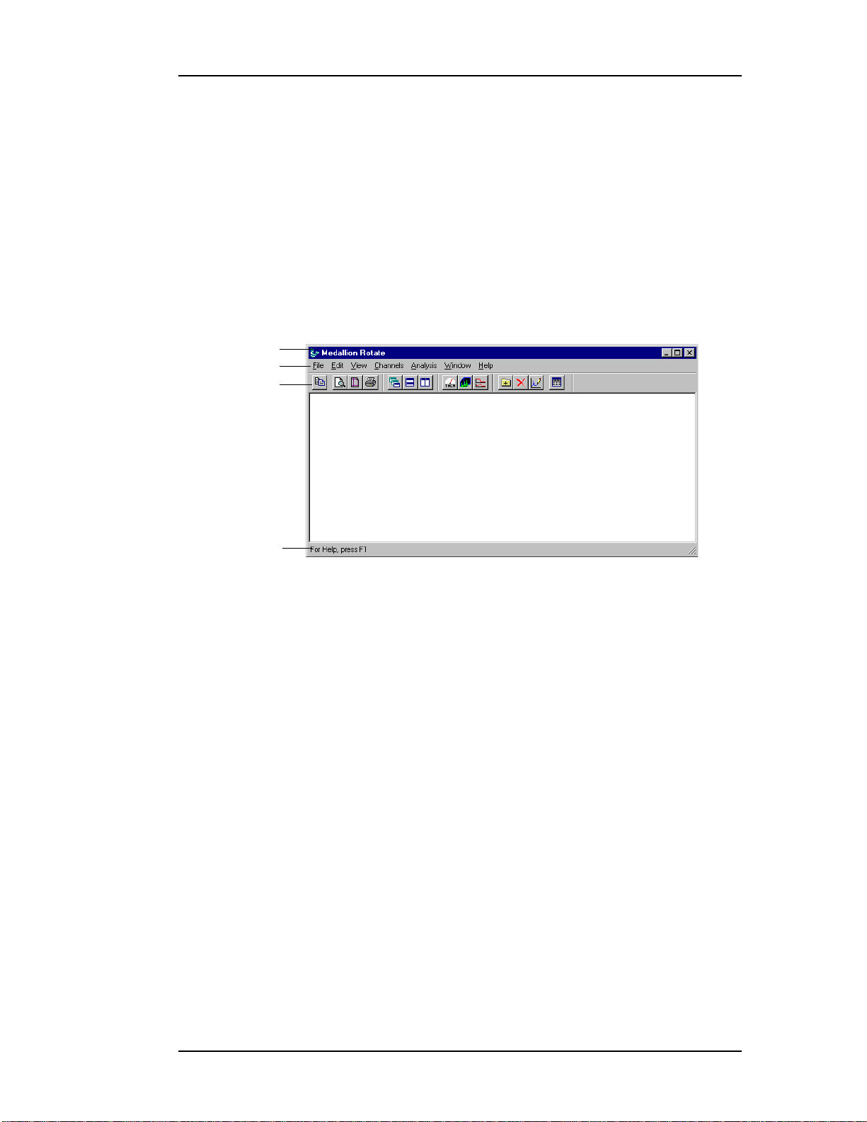
THE MEDALLION ROTATE USER INTERFACE
Medallion Rotate follows the standard Windows¨ user interface standards,
and consists of the usual windows, menus, and toolbars. A picture of the
Medallion Rotate window appears below.
Title bar
Menu bar
Toolbar
Status bar
• The title bar displays the program name.
• The menu bar appears directly below the title bar. It contains the menus
of commands for the program.
• The toolbar appears directly below the menu bar. It contains the tool
buttons that are shortcuts to the most often used functions of the
program. A short ToolTip describing the button function appears when
you move the mouse pointer over a button. You can click and drag a
toolbar to any position within the program window, and “dock” it to
any side of the window. You can also show or hide any toolbar with the
commands on the View menu.
• The status bar shows a brief description of the current command or
button under the mouse pointer.
• Many parts of the program have right-click menus. For example, you
can right-click on a plot window to display a menu of functions for that
plot.
13
Page 14
Medallion Rotate Manual October 2000
• The Channel List window shows the channels (tachometer and data)
that you have imported into, or created in, Medallion Rotate. To display
the Channel List window, right-click anywhere in the Medallion Rotate
program window (except on the menu bar).
• The online help describes each command, dialog box, and plot. To
display the online help, do one of the following:
• Highlight a command on a menu and press F1. This displays an
explanation of the command.
• Open a dialog box and press F1. This displays an explanation of the
controls in the dialog box.
• Make a plot window active by clicking on the plot and press F1.
This displays a description of the functions available for that plot.
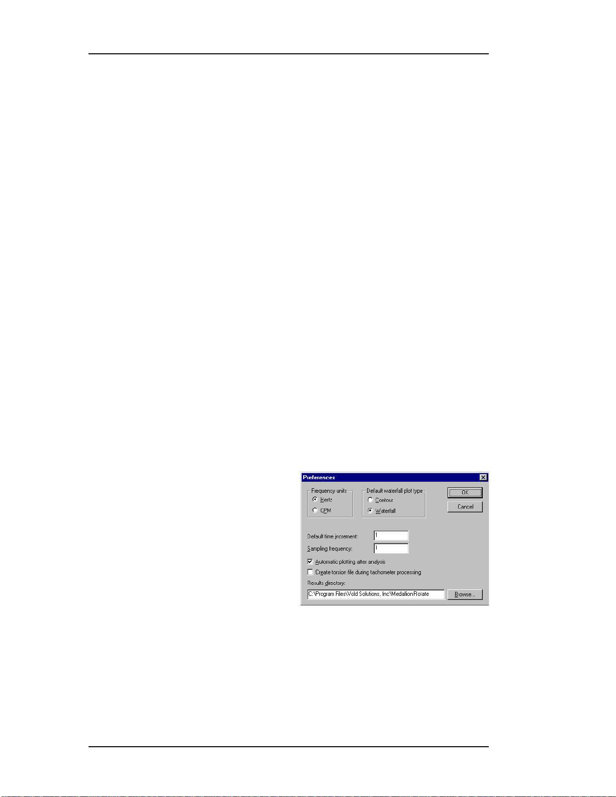
SETTING YOUR PREFERENCES
The preferences settings control the default Medallion Rotate appearance
and functions. These include the following defaults.
• Frequency units in plots
• Waterfall plot type (waterfall or contour)
• Default time increment and sampling frequency
• Automatic plot display after analysis
• Creation of a Torsional analysis file when processing a tachometer
signal
• The directory for the files created by the Medallion Rotate analysis
functions
To set your preferences, follow these steps.
1. Start Medallion Rotate. See “Starting the Software.”
2. From the Edit menu choose
Preferences.
3. In the Preferences dialog box,
select or enter the desired
defaults. Press F1 for a
description of the options.
4. Choose OK when finished.
14
Page 15

October 2000 Medallion Rotate Manual
STARTING MEDALLION ROTATE AND DISPLAYING CHANNELS
The first section of the Tutorial leads you through starting Medallion
Rotate, as well as opening a data file and displaying data channels in the file.
START MEDALLION ROTATE
1. To start Medallion Rotate, click Start, point to Programs, then to
Medallion Rotate, then click Medallion Rotate. The Medallion Rotate
program window appears.
VIEW THE CHANNEL LIST
Medallion Rotate displays the
Channel List window when it starts.
Initially the Channel List shows the 2
channels of data from the demonstration
data file.
Hint: Don’t worry if the Channels
List window is empty, or contains different files than the ones shown in
the picture. Adding files to the Channel List window is described below.
2. You can hide the Channel List window by clicking anywhere on the
Medallion Rotate window or by pressing Esc.
3. You can restore the Channel List window by doing one of the following:
• Right-click on the Medallion Rotate window.
• Press Ctrl+L.
• Click the Channel List
button .
• From the Channels menu
choose Channel List
Window.
REMOVE CHANNELS FROM THE CHANNEL LIST
Removing “channels from the Channel List window does not delete any
data, and you can add the channels back in at any time.
4. Select the 2 channels in the Channel List by holding down the Ctrl key
and clicking the two channels. You can also hold down the Shift key
and select a range of channels.
5. Press Del.
Hint: You can also right-click a
channel and choose Remove.
Note that this removes all
selected channels, not just the
one you right-clicked.
15
Page 16
Medallion Rotate Manual October 2000
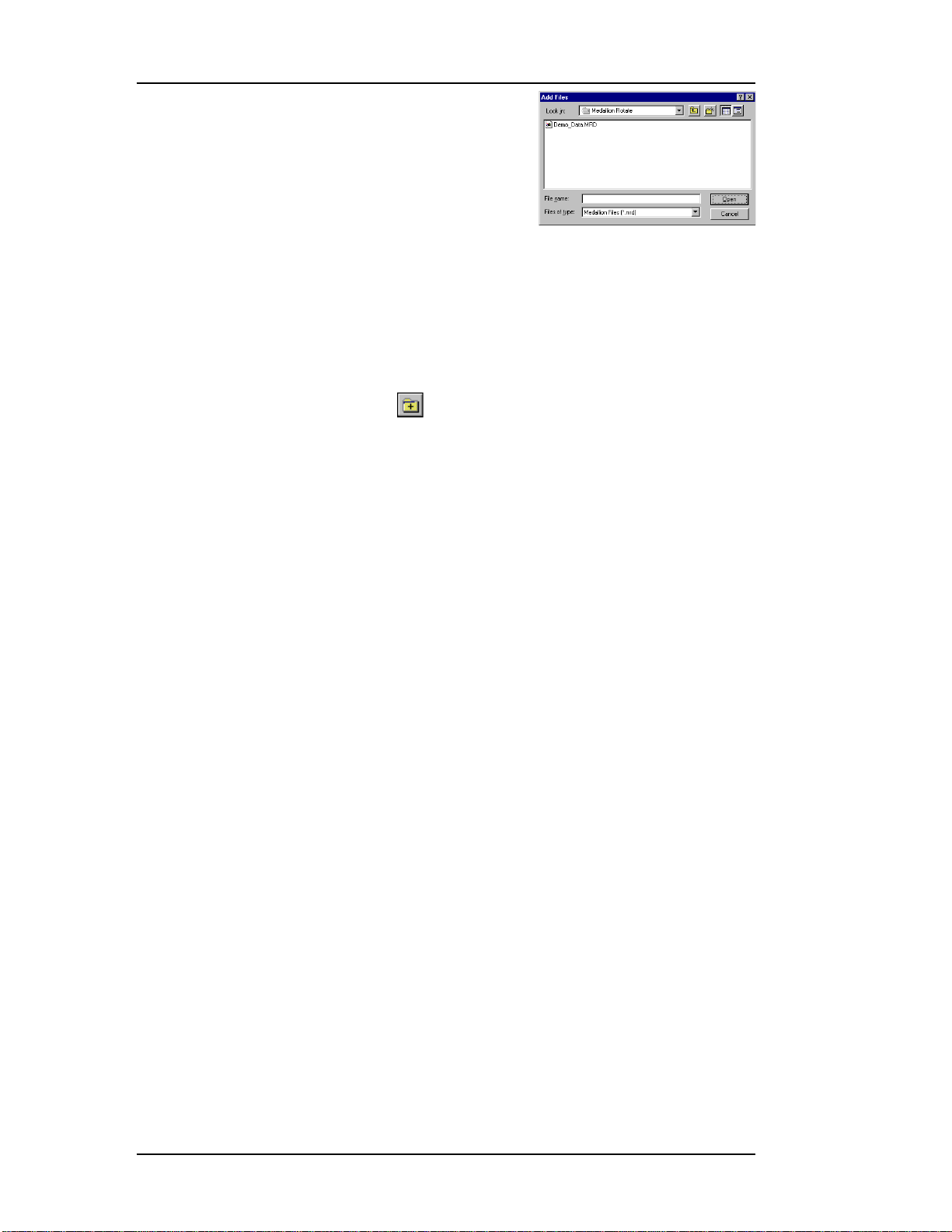
ADD A DAT A FILE
Adding a data “file displays all the channels
of data from that file. Medallion Rotate can display
the channels from a number of different file
formats.
6. Right-click on the Channel List and choose
Add File.
7. Select the correct Files of type. If you don’t know the file type, select
All Files (*.*). For this example, select Medallion File (*.mrd).
8. Select the Demo_Data.MRD file and choose Open. The data channels
from the data file appear in the Channel List (Channel 1, Channel 2).
Hint: You can also do one of the following to add a file:
• Click the Add File button
• From the Channels menu choose Add File.
.
16
Page 17

October 2000 Medallion Rotate Manual
DISPLAYING DATA AND PROCESSING A SIGNAL
The second section of the Tutorial leads you through displaying a time
waveform plot. It then describes the steps to process a tachometer signal to get
the instantaneous machine speed in RPM (revolutions per minute).
The Demo_Data.MRD file contains two channels.
• Channel 1 is a time waveform of a pulse tachometer signal varying
between 0 and 4 Volts.
• Channel 2 is a time waveform from a vibration sensor.
PLOT A TIME WAVEFORM
1. Make sure that Channel 1 is the
only selected channel in the
Channel List window. Then
right-click Channel 1 and
choose Plot. You can also do
one of the following:
• Select the channel and click the Plot button .
• Double-click the channel.
• Select the channel and choose Plot from the Channels menu.
Medallion Rotate displays a plot of the time waveform.
ZOOM IN ON THE TIME WAVEFORM
2. Right-click the plot and choose
Zoom.
3. Click and drag the mouse over a
part of the plot to enlarge that
part of the plot.
The plot redraws the zoomed part
when you release the mouse button.
Note the signal amplitude is from -0.5 to
4 Volts.
4. Right-click the plot and choose
Auto-scale to show the whole signal again.
17
Page 18

Medallion Rotate Manual October 2000
PROCESS A TACHOMETER SIGNAL
Channel 1 should still be selected in the Channel List window. Channel 1 is
a tachometer signal; you can process it to get the instantaneous RPM. You do
not have to display the Channel List window again.
5. Click the Tachometer Processing button
Tachometer Processing command from the Analysis menu.
6. Make sure the Trigger Level is
between 1 and 4 Volts. In general,
the trigger level should be in the
middle of the amplitude of the
tachometer signal for a pulse
tachometer. Choose OK to process
the tachometer signal.
Medallion Rotate displays a plot
of the machine RPM. There are actually
two curves on the plot. One is the
smoothed (spline-fit) RPM curve. The
other is the Raw RPM curve before
Medallion Rotate applied the spline-fit
to smooth the RPM curve.
7. Zoom in on the peak of the
RPM curve to see the two
curves. Right-click the plot,
choose Zoom, then click and
drag over the region you want
to zoom.
. You can also choose the
The smooth curve is the spline-fit
RPM curve, while the jagged curve is
the raw RPM curve before smoothing.
8. Click the Channel List
button or press Ctrl+L to
display the Channel List
window. Note that there are two
new generated files in the
Channel List, each with one
channel. Medallion Rotate
created and saved these files in
the Results directory (see
“Manage Files” to set the
Results directory).
• The smoothrpm0.spl file is the smooth (spline-fit) RPM data.
• The rpm0.raw file is the Raw RPM data.
18
Page 19

October 2000 Medallion Rotate Manual
OTHER TYPES OF ANALYSES
You can perform many other types of analyses in Medallion Rotate to
assist in diagnosing a variety of difficult problems.
• Refer to Chapter 3 “Medallion Rotate Applications” for more
information on the different types of analyses and their uses.
• Refer to Chapter 4 “Medallion Rotate Plotting Features” for more
information on using the plotting functions to manipulate plots.
EXPORTING A CHANNEL AND FILE MANAGEMENT
The third section of the Tutorial describes the process of exporting a
channel to a Universal File Format (UFF) file. It also describes channel and file
management. Medallion Rotate can generate a large number of files during an
analysis, and it is important to manage them so that you do not fill up the
Medallion Rotate directory with unnecessary files.
EXPORT A CHANNEL TO A UFF FILE
Exporting a channel to a UFF file provides 2 useful functions:
• It creates a new ASCII or binary data file in a widely-accepted format.
• It allows you to export only a part of the file instead of the entire file.
For example, the original file might contain 6 hours of data, but you can
export just the 5 minutes of data that contain the desired event.
1. Right-click a channel and choose Export.
2. Enter the file name and choose Browse to
select the directory. Choose Export.
Hint: You can also select a channel and choose
the Export command from the Channels
menu.
RENAME A GENERATED CHANNEL
Medallion Rotate generates one or more channels each time you perform
any type of analysis. Medallion Rotate automatically names a generated
channel by combining the channel name and the data file name. Renaming a
generated channel can help you remember the purpose or parameters of that
analysis.
Note that you can only rename generated channels. You cannot rename
channels from an original data file.
1. Right-click a channel and
choose Rename Channel.
2. Enter the new name for the
channel and press Enter.
Hint: You can also select a channel
and choose the Rename
command from the Channels menu.
19
Page 20

Medallion Rotate Manual October 2000
RENAME A GENERATED DATA FILE
When you perform an analysis, Medallion Rotate generates a data file for
each generated channel. Medallion Rotate automatically names generated files,
but you can determine the type of the file from the file name (Raw RPM, smooth
RPM, waterfall, É). Renaming the generated file can help you remember the
purpose of the analysis or the original data file.
Note that you can only rename generated
files. You cannot rename an original data file.
1. Right-click the generated channel for the desired file and choose
Rename File.
2. Enter the new name for the file and choose OK.
Hint: You can also select a channel and choose the Rename File command
from the Channels menu.
MANAGE FILES
As mentioned above, Medallion Rotate can generate a large number of files
during an analysis. Managing your files in a logical manner can make it much
easier to keep the generated files with the original data files, and to delete files
that you no longer need.
The easiest way to manage files in Medallion Rotate is to use a separate
directory for each set of original data files. Then you can create a new directory
for each set of analyses. Alternatively. you could use the same directory for all
your analysis if you delete all the files after you are done with the analysis.
1. Create a directory for the project. The directory can be anywhere on
your computer or network, but you must have read/write permissions
for the project directory (if on a network).
2. Copy your original data files for the analysis into the project directory.
3. In Medallion Rotate, from the Edit menu choose Preferences.
4. Edit the Result(s) directory so that it is the project directory or a subdirectory of the project directory. Click Browse to select the Result(s)
directory.
5. Perform the analysis. Medallion Rotate stores the generated files in the
Result(s) directory. This makes it easy to keep all the files for a project
together.
6. When you are done with your analysis, you can delete the generated
files if you do not want to keep them.
CAUTION!
Make sure you do not delete your original data files by accident!
20
Page 21

October 2000 Medallion Rotate Manual
CHAPTER THREE
MEDALLION ROTATE APPLICATIONS
This chapter describes the analysis methods available in Medallion Rotate.
The chapter begins with some notes on collecting data. It then lists some uses
for each method, then goes on to present a sample application of the method.
You can use this chapter as a guide to selecting the best method to analyze
data for a particular type of problem. However, this chapter is not meant to be
the last word on analysis using Medallion Rotate. You are likely to discover
other applications for Medallion Rotate after you have been using it for a while.
NOTES ON COLLECTING DATA
SAMPLE RATE
Guidelines for the sample rate for each type of application are described
under the application. One thing to note is that the sample rate of the
tachometer signal does not have to be the same as the sample rate for a data
channel. For example, the sampling rate on the tachometer channel can be much
higher than the sampling rate on a vibration transducer channel.
In general, the sampling rate must be at least 2.5 times the maximum
frequency of interest to avoid aliasing effects (described below). Note that most
analyzers require that you use the sample rate, not the maximum frequency, in
setting up to collect time waveform data. So for a maximum frequency of 400 Hz,
set the sampling rate at 1000 samples/second.
400 Hz <
400 Hz x 2.5 < 1000 = Sampling rate
1000
2.5
Sampling rate
=
2.5
21
Page 22

Medallion Rotate Manual October 2000
ALIASING
Aliasing is an artifact of collecting data caused by using a sampling rate
that is less than twice as high as the highest frequency sampled. Aliasing
results in extra spectral peaks from higher frequencies that get “folded back” by
the signal processing. Most data collection instruments use a low pass filter,
called an anti-aliasing filter, to exclude frequencies that would cause aliasing.
Some instruments that can capture a time waveform (time history) signal do
not include anti-aliasing filters. With this type of equipment, you must be
careful when analyzing spectra, since there may be extra spectral peaks due to
aliasing.
The following example shows a Waterfall plot with aliasing. This torque
data was collected without anti-aliasing filtering. In this plot, speed is
increasing, as you can see by the rising frequency in the cursored spectral
peaks. However, there are several sets of peaks that appear to be decreasing as
speed increases. These are due to alias frequencies “folding back”.
If you were looking at a single spectrum from this data, it would not be
possible to determine which peaks were due to aliasing.
PROCESSING A TACHOMETER SIGNAL
Medallion Rotate can process a tachometer or other machine speed signal
to create an RPM curve that describes the instantaneous speed of the machine
over time. The machine speed signal can be either a pulse or a DC-voltage level
signal from a tachometer, counter, encoder, or other speed sensor.
You can use the speed curve to diagnose some problems directly. You can
also use the speed curve along with other data, such as vibration, as an input
for additional sophisticated Medallion Rotate analysis techniques. Finally, you
can create a torsion file when processing a tachometer signal. See “Torsional
Analysis.”
22
Page 23

October 2000 Medallion Rotate Manual
APPLICATIONS
Processing the tachometer signal results in an RPM curve describing the
instantaneous machine speed. Medallion Rotate uses a spline-fit process to
create a smoothed speed curve from the tachometer signal. The speed curve is
a high-resolution view of the machine speed.
You can use this smooth speed curve to diagnose problems related to the
speed or speed change of a machine. This provides an independent verification
of the machine speed, since some process control indicators suffer from “flat
spots” in their response to speed changes.
Other applications include the following:
• Examining the effects
of changing load or
other process dynamic
on the speed.
• Determining the effect
of power fluctuations
(brownouts) on the
speed.
• Speed profiling on a
multi-drive machine to
determine if there slip at any of the drive units (over- or under- speed).
• Threading analysis on a sheet mill.
• Evaluating the actual machine speed against the ideal constant speed.
• Verification of the speed change between two points to determine the
elongation of the material, such as in a rolling mill.
• Examination of the speed curve to diagnose speed oscillation due to a
loose coupling, hunting motor, or other cause.
INPUT SIGNAL REQUIREMENTS
The input signal to the tachometer analysis is a tachometer or other
machine speed signal. As with all analysis techniques, the better the input
signal, the clearer the results—so a good, clean tachometer signal is essential.
For a pulsed tachometer signal (non-contact probe, encoder, …) the
sampling rate must be at least 2.5 times the maximum frequency of interest to
avoid aliasing effects. A good rule of thumb is to use 5–10 time oversampling of
the tachometer pulse frequency (not the machine speed) to get good, clean
tachometer pulses. For example, if a tachometer produces one pulse per
revolution on a 600 RPM machine, sample the tachometer data at a rate of 50–
100 samples/second (Hz).
600 RPM x
For a DC voltage tachometer signal, you must know the machine speed
when the signal is at 0 volts. For some sensors, the DC speed signal falls to 0
volts before the machine is at a standstill.
1 minute
60 seconds
23
Page 24

Medallion Rotate Manual October 2000
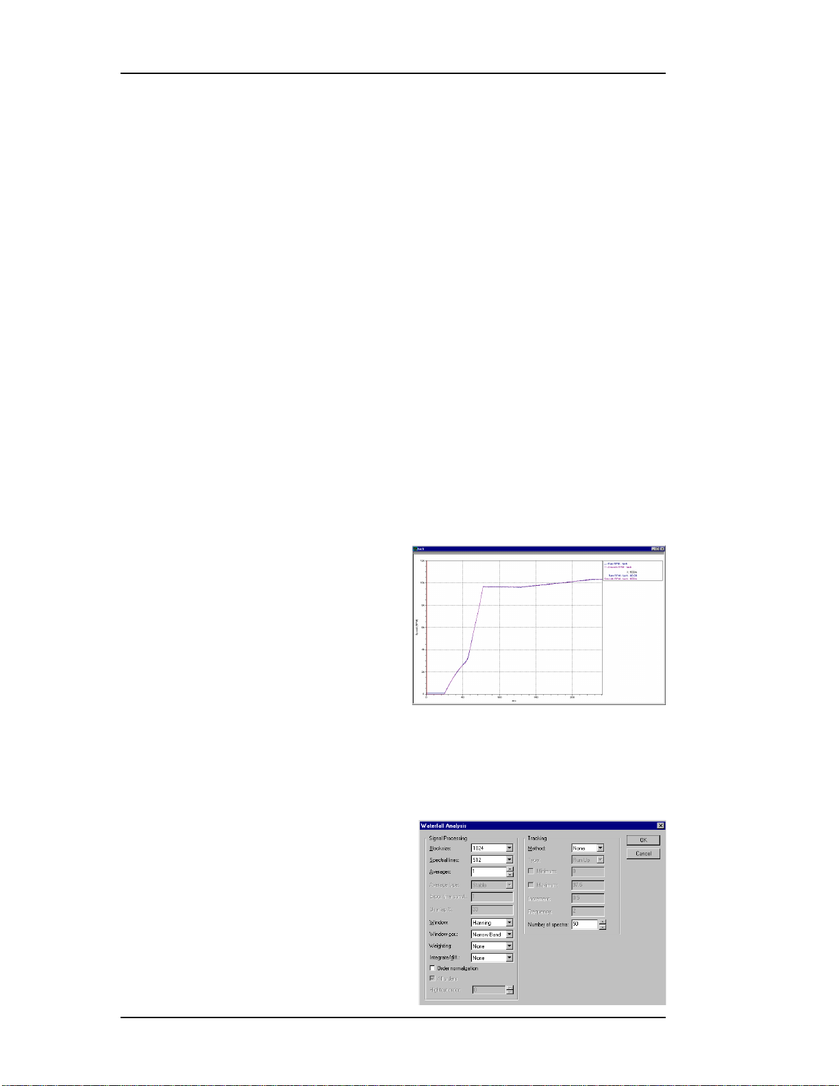
EXAMPLE
The following example is taken from a rolling mill. As the sheet of metal is
rolled out, the speed of the sheet increases. This produces a distinctive speed
profile, as shown in the data collected from several stands along the mill.
This plot is the raw DC tachometer signal.
1. The first step is to process the tachometer signal to create a smoothed
speed curve. For the steps to process a tachometer signal, see “Process
a Tachometer Signal.”
2. Repeat the first step to get smoothed speed curves for each stand.
3. Overlay the speed curves from different stands to see the speed profile
for the machine. You can overlay multiple speed curves by selecting
them in the Channel List window then clicking the Plot button.
THEORY
Medallion Rotate uses a spline-curve fit algorithm that computes raw or
initial estimates of a machine’s instantaneous rotating speed by utilizing
sampled analog data from the sensor. With pulse tachometer data, Medallion
Rotate computes an initial estimate by measuring the time between pulses. Next,
it uses a series of cubic splines that enforce continuity at their boundaries to
create a smooth estimate of the machine’s rotating speed.
x 5 = 50 samples/second
Medallion Rotate then uses a unique technology to remove the “outliers”
from the raw estimate before re-evaluating the spline fit. This allows you to use
noisy tachometer signals or tachometer signals with dropouts. In some cases,
this can delay the need to repair or replace the tachometer.
24
Page 25

October 2000 Medallion Rotate Manual
WATERFALL ANALYSIS
You can perform a Waterfall analysis
on time waveform data from any
transducer. The data transducer can be a
vibration sensor (accelerometer, velocity
sensor, non-contact probe) or any other
meaningful sensor (temperature,
thickness, pressure, …).
You can use Waterfall analysis on a
data channel without a machine speed signal; however, you will not be able to
use the machine speed or order tracking
capabilities of the Waterfall plot. If you
have a tachometer signal you can create
the smooth speed curve as described in
“Processing a Tachometer Signal.” Then
you can combine the speed curve with
data from a correlated transducer in the
Waterfall analysis.
The result of the Waterfall analysis is
a series of spectra displayed on a three-dimensional (X-Y-Z) plot. The Waterfall
plot provides several useful ways of
looking at the data:
• The plot cursors can track the X
axis or the Z axis.
• You can choose frequency or
orders for the X axis and X axis
cursors.
• You can choose spectrum number,
RPM, or seconds for the Z axis and Z axis cursors. If you use order
normalization, you can also choose the number of revolutions for the Z
axis.
• You can display the data in a traditional spectral Waterfall plot, or as a
Color Contour plot. See “Contour Plot.”
Medallion Rotate can also order normalize the data so that the order-related
peaks line up exactly on the orders (when the X axis is in orders). See “Order
Normalization.”
25
Page 26
Medallion Rotate Manual October 2000
APPLICATIONS
The Medallion Rotate Waterfall plot is ideal for non-steady state processes
such as variable speed machinery. The plot shows you the change in the
appearance of the spectra over time. This is particularly useful in the following
applications:
• Analyzing the machine’s behavior during run-up or coast-down.
• Diagnosing amplitude modulation (“beat”).
• Determining the frequency and severity of resonances, such as shaft
critical speeds.
• Analyzing a machine’s response to speed or load variations.
• Isolating non-varying spectral peaks (such as those caused by electric
power or resonance) from speed-dependent peaks (such as vibration).
• Isolating spectral peaks from other processes that are linked to the
machine.
• Ruling out spurious spectral peaks caused by aliasing when using timecapture equipment that does not have anti-aliasing filtering. See
“Aliasing.”
• Performing Waterfall analysis directly on a DC speed signal to diagnose
torsional problems. For more on torsional analysis, see “Torsional
Analysis.”
INPUT SIGNAL REQUIREMENTS
Medallion Rotate Waterfall analysis
requires a smoothed speed curve from
performing a Tachometer analysis if you
want to use the order tracking features of
the Waterfall plot. When collecting the
non-tachometer data (vibration,
temperature, …), note the following:
• If you want to see low frequency
data in the Waterfall analysis, make sure that the high pass filter setting
in your analyzer is not excluding the desired low frequencies.
• The sample rate in the analyzer must be at least 2.5 times the maximum
frequency of interest to avoid aliasing.
• The choice of window function for
analysis depends on the type of
resolution you need (amplitude or
frequency resolution).
26
Page 27

October 2000 Medallion Rotate Manual
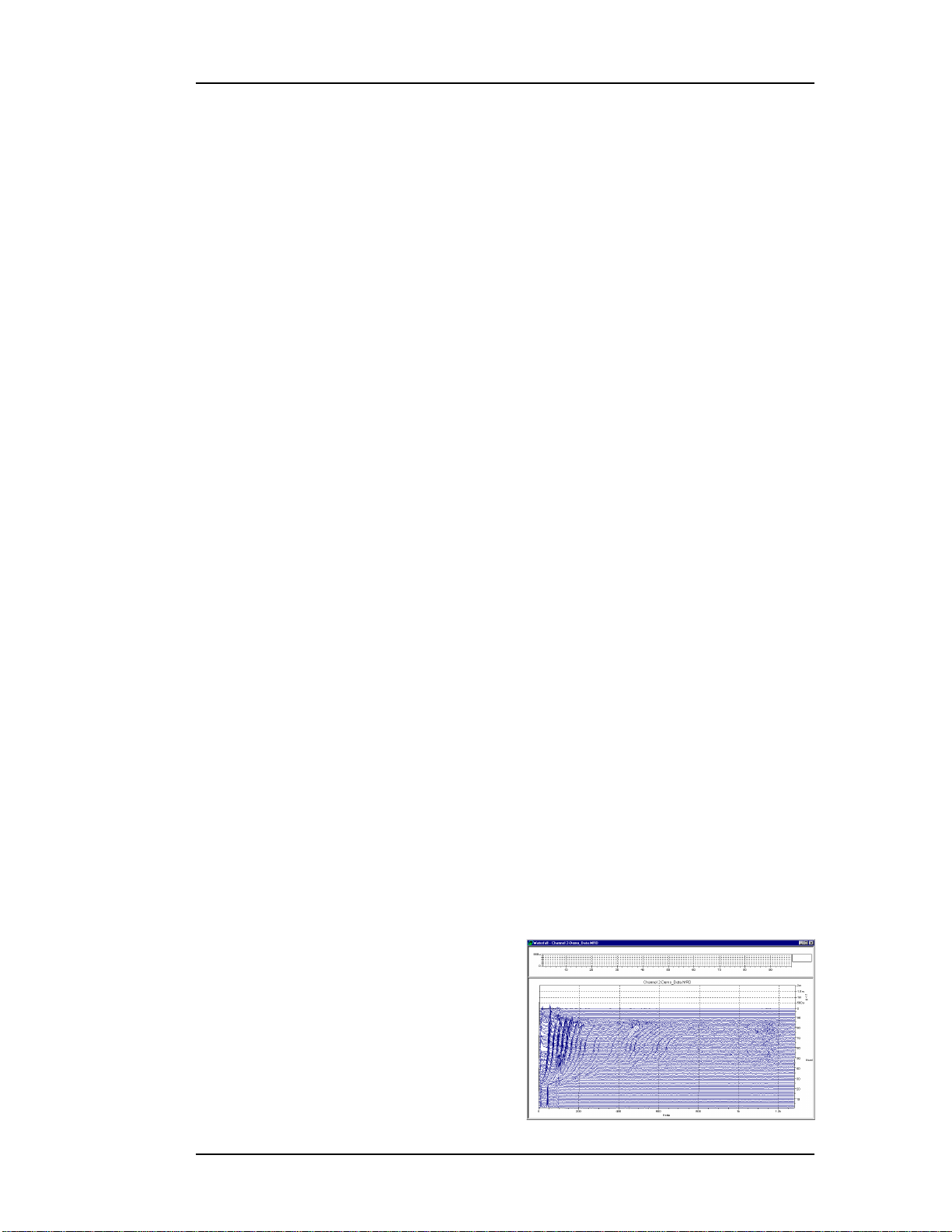
EXAMPLE
The following example is from a turbine.
1. Process the tachometer signal to get the smoothed speed curve. See
“Process a Tachometer Signal.” If you do not have a tachometer signal,
skip this step.
2. Use Waterfall analysis to create the Waterfall plot. In order to use the
order tracking features, select both the smoothed machine speed curve
and the data channel in the Channel List window. If you do not have a
tachometer signal, select the data channel. Then do one of the
following:
• Click the Waterfall analysis button
• Choose Waterfall Analysis from the Analysis menu.
3. Press F1 for an explanation of the dialog box. After selecting the desired
parameters, choose OK to display the Waterfall plot.
.
27
Page 28

Medallion Rotate Manual October 2000
In this Waterfall plot, there are
cursors at 0.5 1, 1.5, and 2 orders. The 0.5
order cursor highlights a turbine rub that
“locks” onto one of the shaft critical
frequencies and then deviates from the 0.5
order cursor.
THEORY
The Medallion Rotate Waterfall
analysis uses the standard Fast Fourier transform to calculate the array of FFT
spectra and then display them in a Waterfall or Color Contour plot
(spectrogram). The spectrum calculation allows for standard parameters such as
blocksize, averaging, windowing, weighting (A, B, and C), frequency domain
integration, and integration/differentiation functions as found on most
spectrum analyzers. Medallion Rotate can display spectra as a function of
either time or RPM.
28
Page 29
October 2000 Medallion Rotate Manual
RPM FROM WATERFALL
The RPM from Waterfall function in Medallion Rotate Plus allows you to
determine the machine speed from a waterfall file. If you do not have a
tachometer signal, or the signal is extremely noisy, you can use other data to
create an RPM curve that describes the speed of the machine over time.
Medallion Rotate can use this smoothed speed curve in the same ways as
a speed curve generated from a tachometer signal. You can use this speed
curve to diagnose some problems directly. You can also use the speed curve
along with other data, such as vibration, as an input for additional
sophisticated Medallion Rotate analysis techniques.
APPLICATIONS
The RPM from Waterfall function is applicable when you have a time
waveform from a data channel, but no tachometer signal or a noisy signal.
There may not be a tachometer available, or it may be impractical to use a
tachometer or other speed sensor on the machine. In some cases, the RPM from
Waterfall function may produce a better speed curve than a tachometer.
INPUT
When collecting the non-tachometer data (vibration, temperature, …), note
the following:
• If you want to see low frequency data in the Waterfall analysis, make
sure that the high pass filter setting in your analyzer is not excluding
the desired low frequencies.
• The sample rate in the analyzer must be at least 2.5 times the maximum
frequency of interest to avoid aliasing.
• The choice of window function for analysis depends on the type of
resolution you need (amplitude or frequency resolution). Since the
RPM from Waterfall function depends more on the position of the
spectral peaks than on the amplitude, the Hamming window is a good
default choice.
EXAMPLE
This example uses the RPMFromWaterfallDemo.wat file included with
Medallion Rotate Plus. You can also use any waterfall file generated by
Medallion Rotate using Waterfall analysis (see “Waterfall Analysis” ).
1. In the Channel List Window select
the RPMFromWaterfallDemo.wat
file, then select the waterfall
channel. You can display the
Waterfall by clicking on the Plot
button.
29
Page 30

Medallion Rotate Manual October 2000
2. From the Analysis menu,
choose RPM from Waterfall.
This displays a color contour
plot of the waterfall.
3. Enter the order you want to use
to find the machine speed. For
this example, leave the value at
1 for the first order.
4. Zoom in on the area around the first order.
5. Working from the bottom of the
plot to the top, click the peaks
for the order. Medallion Rotate
Plus draws a line for the order
by estimating the location of
the order. You can change the
location of the line by clicking
on the plot.
If you want to start over, simply choose Cancel.
6. When the line on the plot connects the peaks for the order, click OK.
Medallion Rotate Plus calculates a smoothed machine speed curve
based on the order number and
the line on the plot.
7. You can select the smoothed
speed curve and the waterfall
data in the Channel List
window, then click the Plot
button to display the Waterfall.
This allows you to use the
order tracking features of the
Waterfall plot.
THEORY
The RPM from Waterfall function
uses the assumption that an order of
running speed generates a distinct series of peaks in a Waterfall plot. After you
identify the peaks for the order, Medallion Rotate Plus determines the RPM
versus time function and generates a smooth RPM curve of the instantaneous
speed.
30
Page 31

October 2000 Medallion Rotate Manual
COMPUTED ORDER TRACKING
Computed Order Tracking uses the smooth speed curve from processing a
tachometer signal or from the RPM from Waterfall function. You can combine
the speed curve with data from a correlated transducer to perform a Computed
Order Tracking analysis. The correlated transducer can be an vibration sensor
(accelerometer, velocity sensor, non-contact probe) or any other meaningful
sensor (temperature, thickness, pressure, …).
APPLICATIONS
Computed Order Tracking shows you the amplitude and phase of the data
at selected orders, plotted against the machine’s speed. Computed Order
Tracking is ideal for variable speed machinery. This is particularly useful in the
following applications:
• Analyzing of the machine’s behavior during run-up or coast-down.
• Analyzing of a machine’s response to speed or load variations.
• Determining the frequency and severity of resonances, such as shaft
critical speeds, even when the resonances are heavily damped.
• Balancing rotors.
• Generating operating deflection shapes. For more on operating
deflection shapes, see “Exporting Calculated Orders Data to
ME’scope.”
INPUT SIGNAL REQUIREMENTS
Medallion Rotate Computed Order Tracking requires a smooth speed curve
from processing a tachometer signal or using the RPM from Waterfall function.
Medallion Rotate processes the machine speed with the transducer data to
create the plot of the orders. When collecting the non-tachometer data
(vibration, temperature, …), note the following:
• If you want to see low frequency data in the Order Track plot, make
sure that the high pass filter setting in your analyzer is not excluding
the desired low frequencies.
• The sample rate in the analyzer must be at least 2.5 times the maximum
frequency of interest to avoid aliasing. Be aware that the anti-aliasing
filter in many data collection instruments truncates the upper 20-30% of
the frequency range (the highest orders in the signal).
• The choice of window function for analysis depends on the type of
resolution you need (amplitude or frequency resolution).
31
Page 32

Medallion Rotate Manual October 2000
EXAMPLE
This example is from the demonstration data included with Medallion
Rotate.
1. Process the tachometer signal to
get the smoothed speed curve.
See “Process a Tachometer
Signal.”
2. Then use Computed Order
Tracking to get the order data.
Select both the smoothed
machine speed curve and the
data channel in the Channel List
window, then do one of the
following:
• Click the Computed Order Tracking button
• Choose Computed Order Tracking from the Analysis menu.
3. Press F1 for an
explanation of the dialog
box. After selecting the
desired parameters,
choose OK to display the
Bode plot of the orders.
THEORY
The order functions created by the Computed Order Tracking function are
leakage free because the instantaneous machine speed controls the resampling
in the Computed Order Tracking algorithm. Computed Order Track plots are
created from many more data points than the orders plotted in a Waterfall, and
are a more precise picture of each order.
.
32
Page 33

October 2000 Medallion Rotate Manual
TORSIONAL ANALYSIS
Medallion Rotate can process a tachometer or other machine speed signal
to create an accurate kinematic description of torsional vibrations from a single
measurement. The machine speed signal must be a pulsed signal from a
tachometer, counter, encoder, or other speed sensor that shows torsional
changes.
Note:Torsional analysis creates a time history of the machine speed, similar
to that from a high-resolution DC speed sensor. If you have a highresolution DC speed signal, you can simply perform a Waterfall analysis
on the speed signal to view the torsional vibration. See “Waterfall
Analysis.”
Torsional analysis results in a time history of instantaneous shaft speed
with even sample spacing in time (in revolutions per second). You can then use
Waterfall analysis of the torsion file to create a series of spectra displayed on a
three-dimensional (X-Y-Z) plot. The Waterfall plot provides several useful ways
of looking at the data:
• The plot cursors can track the X axis or the Z axis.
• You can choose frequency or orders for the X axis and X axis cursors.
• You can choose spectrum number, RPM, or seconds for the Z axis and
Z axis cursors.
• You can display the data in a traditional spectral Waterfall plot, or as a
Color Contour plot. See “Contour Plot.”
You can use the torsional Waterfall plot to diagnose a variety of problems
directly from the machine speed signal. In some cases, Medallion Rotate can
eliminate the need for slip rings, telemetry, and torsional transducers.
APPLICATIONS
Torsional analysis is useful in diagnosing any problems arising from
torsional vibration (variations in rotational speed of a component due to
twisting). This technique can identify problems that do not usually appear in
conventional vibration measurement and analysis. This is particularly useful in
the following applications:
• Finding shaft critical speeds in turbines.
• Identifying torsional resonances in internal combustion engines that
reduce the efficiency.
• Identifying torsional resonances in reciprocating machinery.
• Diagnosing the cause of gear “chatter” from torsional vibration.
33
Page 34

Medallion Rotate Manual October 2000
INPUT SIGNAL REQUIREMENTS
The fixed sampling rate for the machine speed signal must be high enough
to give a good definition of pulses. Note that the number of tachometer pulses/
revolution determine the maximum torsional frequency of the analysis. In
addition, the sampling rate must be at least 2.5 times the maximum frequency of
interest to avoid aliasing effects. For example, for a maximum torsional
frequency of 10 orders, you must have a tachometer capable of providing at
least 2.5 x 10 pulses/revolution (25 pulses/revolution).
A good rule of thumb is to use 5–10 time oversampling of the tachometer
pulse frequency (not the machine speed) to get good, clean tachometer pulses.
For example, for a tachometer that produces 25 pulses per revolution on a 60
RPM machine, sample the tachometer data at a rate of 125–250 samples/second.
25 pulses/rev x 60 RPM x
Since the torsional analysis algorithm works in the time domain, do not use
aggressive anti-aliasing filters for the data acquisition.
EXAMPLE
This example is from a 3-cylinder
diesel engine. The data is from a noncontact sensor on a 72-teeth gear.
1. The first plot is the time waveform,
zoomed in to show more detail. To
display a time waveform, select the
tachometer channel in the
Channels List window and click
the Plot button.
2. Set the preferences to create the torsion file.
• From the Edit menu choose Preferences.
• Select Create torsion file during tachometer processing so Medallion
Rotate will create the torsion file.
• Medallion Rotate also uses the sampling rate from this dialog box when
processing the signal. This is not the same as the original sample rate
used when collecting the data. A
meaningful sample rate is 1/5 the
rate of the tachometer signal. For
example, for a 1 Hz tachometer
signal, use a sample rate of 0.2 Hz
when processing the tachometer
signal.
1 minute
60 seconds
x 5 = 125 samples/second
34
Page 35

October 2000 Medallion Rotate Manual
3. Choose OK to close the Preferences dialog box.
4. Process the tachometer signal. See “Process a Tachometer Signal.”
Medallion Rotate creates the torsion file at the same time, then displays
the machine speed curve. Note this is the instantaneous speed in
degrees/second. The machine speed curve shows the torsional speed
changes as oscillations around the mean speed.
Hint: After processing, choose Preferences from the Edit menu. Clear the
check box for Create torsion file during tachometer processing unless
you are going to create more torsion files immediately. Creating the
torsion file during Tachometer processing can slow down Medallion
Rotate.
5. Close or minimize the machine
speed plot.
6. In the Channel List window, select
the torsion file (*.tor) and the
smoothed speed curve, then click
the Waterfall analysis button to
create a Waterfall plot. The
amplitude axis for the plot is in degrees/second.
Note that the torsional file includes a large DC component, equal to the
mean machine rotational speed. The amplitude of the DC component is much
greater than that of the higher order torsional vibration components, and must
be excluded.
7. Right click on the plot and select
Zoom. Then click and draw a
rectangle on the plot that excludes
the DC component. See “Zoom in
on the Time Waveform.”
8. Right click on the plot and choose
Properties. Select Viewed data
only in the Amplitude Axis tab of
the dialog box to scale the
amplitude axis to the zoomed part
of the plot. Note that the torsion
Waterfall plot shows the firing
order at 1.5 orders, and that in
general, the torsional component
driven by the firing orders is lower
at higher speeds. The first order is
the crankshaft imbalance, which increases with increasing speed. The
other peaks are harmonics of the firing order.
There is also a resonance as shown in the second plot.
Hint: To change between frequency and order cursors, right click the plot
35
Page 36

Medallion Rotate Manual October 2000
and choose Properties. Then select the parameter for the cursor under
Track axis on the Cursor tab.
You can also use spline-fit machine speed curve produced by Tachometer
analysis to display the torsional orders.
1. Display the Channel List window.
2. Select the torsional file (*.tor) and the smoothed spline-fit file (*.spl).
and click the Computed Order Tracking button. For this example,
displaying the 1.0 and 1.5 orders
shows the firing order and the
imbalance. The upper curve on the
lower plot shows the firing order,
and the lower curve shows the
imbalance. Note the amplitude of
the firing order curve decreases
with increasing speed.
3. Running the Computed Order Tracking again using more orders, and
setting the X axis to frequency shows all the peaks lining up at the
resonant frequency.
THEORY
Torsional vibration causes small
variations in the speed of a rotating
component. These variations can be
detected in the speed signal from the
component, provided that the signal
provides sufficient resolution. Medallion
Rotate processes the speed signal, and converts the variations in speed to the
frequency domain. This generates a time history of the speed as a DC signal. If
the original tachometer signal contains N pulses/rev, Medallion Rotate can
extract torsional orders up to N/2 orders.
36
Page 37

October 2000 Medallion Rotate Manual
ORDER NORMALIZATION
Medallion Rotate Plus can resample a time waveform to order normalize the
data when performing a Waterfall analysis. Order normalization cancels the
effect of frequency smearing across spectral bins when the shaft speed is
changing rapidly (high slew rate). Order normalization ensures that orderrelated peaks are properly aligned when plotted against the orders.
Order normalization also allows you to use a smaller blocksize when
performing the Waterfall analysis. This can significantly shorten processing
time while maintaining good frequency and amplitude resolution.
APPLICATIONS
Order normalization is ideal for identifying order-related frequencies in the
Waterfall plot. Order-related frequencies are located at the running speed of the
component and multiples of the running speed. The running speed is the first
order. This is particularly useful when attempting to separate order-related and
non-order-related peaks in the Waterfall plot. Since the X axis is displayed in
orders, it is easy to pick out the order-related peaks.
INPUT SIGNAL REQUIREMENTS
Order normalization requires a smoothed speed curve from performing a
Tachometer analysis or using the RPM from Waterfall function. Medallion
Rotate Plus processes the machine speed with the transducer data to create the
order normalized Waterfall analysis. When collecting the non-tachometer data
(vibration, temperature, …), note the following:
• If you want to see low frequency data in the Waterfall analysis, make
sure that the high pass filter setting in your analyzer is not excluding
the desired low frequencies.
• The sample rate in the analyzer must be at least 2.5 times the maximum
frequency of interest to avoid aliasing.
• The choice of window function for analysis depends on the type of
resolution you need (amplitude or frequency resolution). The Hanning
window is a good default choice. The Uniform window is only a good
choice when the orders are integer multiples of the shaft speed (1x, 2x,
3x, …).
Order normalization requires a clean tachometer signal for best results.
Processing the tachometer signal must produce a good spline-fit to provide a
smooth speed curve. Note that the resampling algorithm does not require that
the tachometer pulses correlate with the resampling angle.
37
Page 38

Medallion Rotate Manual October 2000
EXAMPLE
This example shows the difference in
the appearance of a Waterfall plot
resulting from order normalization. The
first Waterfall plot does not use order
normalization.
The second Waterfall plot uses order
normalization. Notice that the non-orderrelated peaks have been minimized, while order-related peaks have been
enhanced.
1. To use order normalization when
performing a Waterfall analysis,
first select the smoothed machine
speed and the data channels in the
Channels List window. Then click
the Waterfall analysis button.
2. In the Waterfall analysis dialog
box, select Order normalize. Note
that this is not available if you do not select the smoothed machine
speed in the Channels List window.
3. Select the other desired parameters and choose OK to create the order
normalized Waterfall plot.
THEORY
Medallion Rotate Plus order normalizes the data by resampling it. Time
waveform data is usually collected using a fixed number of samples/second.
This means that more samples/revolution are collected at lower speeds, and
fewer
samples/revolution at higher speeds. Resampling allows Medallion Rotate Plus
to gather a constant number of samples per revolution, regardless of the speed
of the machine.
38
Page 39

October 2000 Medallion Rotate Manual
MILLSTRUM ANALYSIS
Millstrum analysis in Medallion Rotate Plus simplifies the process of
identifying families of harmonics and sidebands. Harmonics are multiples of a
primary frequency, and appear as a series of equally spaced spectral peaks of
increasing frequency. Sidebands are pairs of equally spaced spectral peaks that
appear to both sides of a primary frequency. Sidebands are often caused by
modulation of the primary (“carrier”) frequency by a second frequency.
In some cases, it can be difficult to identify harmonics and sidebands in a
conventional Spectrum plot—particularly in spectra that have many peaks
obscuring the harmonics or sidebands.
Millstrum analysis simplifies the process of identifying harmonics and
sidebands by removing everything that is not harmonic, and presenting the
results in an easily-understood format. Millstrum analysis is similar to using the
cepstrum, but goes further in simplifying the results so that you do not have to
perform any additional calculations. The fundamental frequency and
modulating frequencies appear clearly as peaks in the Waterfall plot from
Millstrum analysis.
APPLICATIONS
Millstrum analysis is ideal for identifying harmonics and sidebands in the
following applications:
• Heavily modulated signals.
• Low amplitude harmonics and sidebands, such as in early-stage
gearbox and bearing faults.
• Signals that produce complicated spectra with peaks obscuring the
harmonics or sidebands.
INPUT SIGNAL REQUIREMENTS
You can use Millstrum analysis on a data channel without a smoothed
machine speed curve; however, you will not be able to use the machine speed
or order tracking capabilities of the Millstrum plot.
Medallion Rotate processes the transducer data to create the Millstrum
analysis. When collecting the non-tachometer data (vibration, temperature, …),
note the following:
• If you want to see low frequency data in the Millstrum analysis, make
sure that the high pass filter setting in your analyzer is not excluding
the desired low frequencies.
• The sample rate in the analyzer must be at least 2.5 times the maximum
frequency of interest to avoid aliasing.
• When there is a tachometer signal, you can use the order domain for
easier identification of the periodic frequencies.
39
Page 40

Medallion Rotate Manual October 2000
• More spectral lines are required for the Millstrum analysis, since the
analysis reduces the number of lines in the result by half. Collect a large
number of sample points, and use the largest possible blocksize for the
signal. This is explained in the section on “Theory” below.
• The choice of window function for analysis depends on the type of
resolution you need (amplitude or frequency resolution). If you are
using order normalization, the Hanning window is a good choice. The
Uniform window is only a good choice when the orders are integer
multiples of the shaft speed (1x, 2x, 3x, …).
EXAMPLE
This example is from an automotive
dynamometer. The first Waterfall plot does
not use Millstrum analysis. Notice the
large number of peaks, and the difficulty in
sorting out the harmonics.
The second Waterfall plot is the result
of the Millstrum analysis. Note that the
peaks show the forcing and the harmonic
frequencies. Remember that the X axis, while in Hz, is not the same as the X axis
in the first Waterfall plot. Instead, you can read the forcing and harmonic
frequencies directly from the X axis.
To use Millstrum analysis, follow
these steps:
1. In the Channel List window, select
the data channel (and a
corresponding smoothed machine
speed curve if desired). Then click
the Waterfall analysis button.
2. In the Waterfall analysis dialog
box, select Millstrum for the Window cor.
3. Select the other desired parameters and choose OK to create the
Millstrum plot.
THEORY
A simple analogy is that Millstrum analysis looks at the spectrum as if it
were a time waveform, and attempts to identify periodic repeating events in the
spectrum. In other words, it takes the FFT of the FFT spectrum. Since both
harmonics and sidebands are periodic repeating peaks in a spectrum, they show
up in the Millstrum as single peaks. The “frequencies” of the peaks in the
Millstrum are the frequencies of the repeating events.
40
Page 41

October 2000 Medallion Rotate Manual
More formally, Millstrum analysis is essentially the Fourier transform of the
logarithm of the absolute value of the frequency spectrum. It identifies
periodicity in the frequency domain. The normal formulation, called the real
cepstrum, has as its abscissa the period of the harmonics, but by inverting
period, the Millstrum displays the results in the frequency domain.
Millstrum analysis uses the logarithm of the frequency spectrum to raise
the low amplitude peaks relative to higher amplitude components of the signal.
This amplifies the presence of low amplitude harmonics, such as those created
by early-stage bearing faults.
For harmonics, the peaks in the spectrum are located at multiples of the
primary frequency. The spacing (or “frequency”) between peaks is the same as
the primary frequency. So harmonics in a spectrum appear as a single peak at
the primary frequency in the Millstrum.
For sidebands, the peaks in the spectrum are located at the primary
frequency plus or minus multiples of the modulating frequency. The spacing
(“frequency”) between the peaks is the same as that of the modulating
frequency. So sidebands appear as a single peak at the modulating frequency.
EXPORTING CALCULATED ORDERS DATA TO ME’SCOPE
Medallion Rotate can export calculated order tracking data to the
ME’scope™ program (Vibrant Technology) for operating deflection shape
analysis. This allows you to see a animation of the machine as it moves in the
coherent pattern of a given order at a given speed.
There are two ways to export calculated order tracking data to ME’scope.
• You can calculate the order tracking data in Medallion Rotate, then
export that data to ME’scope. This is limited to data from only one file.
• You can create measurement sets from one or more data files that share
a common tachometer and reference channel. This automates the
process of calculating the order tracking data, and combines the
channels from the data files into the appropriate files for ME’scope.
APPLICATIONS
By showing you how the machine is moving, ME’scope allows you to
diagnose a variety of problems. For example, it
shows you how a drive train deflects in
response to an engine cylinder firing order. It is
also useful for diagnosing high-cycle fatigue
problems on the spring side of the engine. The
following graphic shows a wire-frame model for
data taken from a tractor engine. The data was
taken on the sub-frame and exhaust system of
the tractor during the tests.
41
Page 42

Medallion Rotate Manual October 2000
ME’scope animates the wire-frame model so that you can view the physical
deflection of the components at specific orders. For more detailed information,
refer to the ME’scope tutorial on the Medallion Rotate Installation CD ROM.
INPUT SIGNAL REQUIREMENTS
The input requirements are the same as for Computed Order Tracking. If
you are going to combine two or more data files for the same machine, all data
files must have a common tachometer channel and reference channel.
EXAMPLE
The first example shows how to export a order tracks for a single order of
data to ME’scope. If you want to export multiple orders, you must export each
one separately. Alternatively, you can use the process outlined in the second
example to export multiple orders at the same time.
TO EXPORT A SINGLE ORDER
1. Perform the steps for Computed Order
Tracking to create the order tracks.
2. Select the desired order track channels from
the Channel List window. Note that all the
selected order tracks must be the same order
(first order, for example). The order tracks are
identified by the channel name (Order 1, Order
2, …).
3. On the File menu point to Export, then choose Orders to ME’scope.
4. In the Export Orders dialog box, select or enter the desired values. Press
F1 for a description of the options.
5. Choose Export when finished. Medallion Rotate exports the selected
order tracks to a format that ME’scope can use.
TO EXPORT MULTIPLE ORDERS OR DATA FILES
The second example describes exporting multiple orders of data from two
or more files. This is useful when you have collected data during two or more
runs on the same machine. The data from each run becomes a measurement set
in Medallion Rotate (one data file = one measurement set). You then export one
or more measurement sets to ME’scope in a single set of steps.
To begin the process of creating and exporting measurement sets, from the
Edit menu choose Measurement Sets. Then choose Create to create the first
measurement set. After completing the information in a dialog box, choose Next
to go to the next step. You can also press F1 for a description of the current
dialog box options.
Medallion Rotate includes demonstration data for export to ME’scope. You
can find a complete tutorial on the process of exporting measurement sets on
the Medallion Rotate installation CD.
42
Page 43

October 2000 Medallion Rotate Manual
CHAPTER FOUR
MEDALLION ROTATE PLOTTING FEATURES
This chapter describes the plots in Medallion Rotate. It covers the general
features of plots that allow you to change the views of the data, as well as how
to save a particular plot setting as the default for that type of plot. It then
describes the individual plots that appear in Medallion Rotate. This chapter
does not describe the applications for each plot. Refer to Chapter 3 ÒMedallion
Rotate ApplicationsÓ for the analyses that produce each type of plot.
43
Page 44

Medallion Rotate Manual October 2000
GENERAL PLOT FEATURES
The plotting features described in this section are common to all of the
plots, unless otherwise noted.
RIGHT-CLICK MENU
To access the plot controls, right-click on the plot to display a menu of
commands.
• Auto-Scale - Set the plot axes to optimally display all the data on the
plot. This is useful after you have used Zoom to examine a part of the
plot in more detail.
• Zoom - Magnify a region defined by clicking and dragging a rectangular
region on the plot. The program enlarges the region to fill the plot
window.
• Orientation - Change the orientation of the plot axes by moving the
mouse pointer then clicking to display the new plot orientation
(Waterfall plot only).
• Add Cursor - Select a cursor type to add to the plot in addition to the
current cursors. The program displays the cursor properties dialog box,
so that you can define the parameters for the cursor.
• Delete Cursor - Delete the current cursor from the plot.
• Cursor Properties - Display the Cursor Properties dialog box for the
current cursor.
• Properties - Display the plot properties dialog box. Click Help to
display the online help explaining the fields in the dialog box. This
dialog box controls the appearance of the plot, including the colors,
labels, axis scaling, and numeric value display.
SELECTING THE ACTIVE TRACE
If the plot contains multiple traces, you can select the active trace by
clicking on the trace. The values displayed in the plot legend and the ToolTips
for the cursors are for the active trace.
SELECTING THE ACTIVE CURSOR
Select the active cursor by clicking on the cursor.
MOVING A CURSOR
You can use either the mouse or the keyboard to move a cursor on a plot.
• Use the mouse by clicking on a cursor and dragging it across the plot.
You can also move a cursor to a different trace by clicking on the trace
near the cursor.
• Use the arrow keys to move the current cursor across the trace. You
must still use the mouse to select a different cursor or plot trace.
Normally the cursor moves from data point to data point along a trace.
• If you hold down the Ctrl key when moving the cursor, the cursor
44
Page 45

October 2000 Medallion Rotate Manual
jumps to the nearest peak in the trace (peak mode).
• If you hold down the Shift key when moving the cursor, the cursor
moves in increments of one-tenth of the distance between data points
on the trace (fine mode).
SAVING THE PLOT APPEARANCE AS THE DEFAULT
The plot Properties dialog box allows you to change the appearance of the
plot in many ways. You display the Properties dialog box by right-clicking on
the plot and choosing Properties. Once you have changed the plotÕs
appearance to your satisfaction, you can save that appearance as the default
for the plot type. Then when you open another plot of the same type, the new
plot has the new default appearance.
Use the plot Properties dialog to change the plot appearance.
From the View menu choose Save Plot Settings as Default.
TIME WAVEFORM PLOT
A Time Waveform plot is simply a plot of the amplitude of a signal in volts
against time in seconds. You might use a Time Waveform plot for the following
purposes:
• To verify that a tachometer channel contains the correct signal.
• To make sure that a channel has good data before proceeding with
analysis.
• To determine the time or duration of a particular event for further
analysis. Some situations require recording hours of data to capture an
event that might occupy only a few minutes of data. By slicing out only
the relevant data, you can significantly shorten analysis time. See
“Export a Channel to a UFF File” for more information.
Right-click a time waveform data channel in the Channel List window and
choose Plot. You can also do one of the following:
• Select the channel and click the Plot button .
• Double-click the channel.
• Select a channel and choose the Plot command from the Channels
menu.
Medallion Rotate displays a plot of the time waveform.
You can overlay time waveforms by selecting two or more time waveform
channels before plotting. Note that you cannot
overlay other types of data on a Time Waveform
plot.
45
Page 46

Medallion Rotate Manual October 2000
RPM (MACHINE SPEED) PLOTS
The plot below shows two RPM curves that display the instantaneous
speed of a machine. You create these curves by performing a Tachometer
analysis on a tachometer or other machine speed signal. See “Processing a
Tachometer Signal.” Medallion Rotate Plus can also create RPM curves without
a tachometer from a Waterfall plot of a data channel. See “RPM from Waterfall.”
To display calculated RPM files, do one of the following:
• You can display a calculated Raw RPM (rpm*.raw file) curve or a
Smooth RPM (smoothrpm*.spl)
curve by right-clicking the
channel in the Channel List
window an choosing Plot.
• You can display both curves
together (as shown above) by
selecting both channels, then right-clicking one and choosing Plot.
WATERFALL PLOT
The Waterfall plot displays multiple spectra as a function of position. You
create a Waterfall plot by performing a Waterfall analysis on data signal, or on
the combination of a data and a machine speed signal. See “Waterfall
Analysis.”
The Waterfall plot also shows an amplitude plot for the “slice” under the
cursor. You can display a waterfall by
right-clicking the waterfall file in the
Channel List window and choosing
Plot.
Hint: Medallion Rotate needs the
smoothed RPM file to display
the waterfall in orders.
• Select both the Waterfall (waterfall*.wat) and the Smooth RPM
(smoothrpm*.spl) channels in the Channel List window. Then right-click
one and choose Plot.
• If you have already displayed a Waterfall plot, you can drag and drop
the Smooth RPM (smoothrpm*.spl) channel from the Channel List
window onto the Waterfall plot. Medallion Rotate recalculates the
waterfall using the smoothed speed curve.
46
Page 47

October 2000 Medallion Rotate Manual
CONTOUR PLOT
The “Contour plot is similar to a Waterfall plot in that it displays multiple
spectra plotted as a function of position. However, the Contour plot uses
contour lines or colors to identify areas of equal amplitude. While the view in a
Waterfall plot is “across” the spectra from the side, the view in a Contour plot is
from “above” the spectra, looking down on the data.
There are two ways to display a Contour plot.
• Display a Waterfall plot, then
from the View menu choose
Change Waterfall Type.
• From the Edit menu choose
Preferences. Set Default
waterfall plot type to Contour.
When you perform a Waterfall analysis or display a waterfall file,
Medallion Rotate uses a Contour plot by default.
ORDER TRACKING PLOT
The Order Tracking plot displays the result of the Computed Order
Tracking analysis in a Bode plot format.The lower plot shows the magnitude
plotted against frequency, time, or machine speed for each order. The upper plot
shows the phase plotted against the frequency, time, or machine speed for each
order.
To display calculated Order traces, do one of the following:
• You can display a calculated Orders (orders*.tra file) curve by rightclicking the channel in the Channel List window an choosing Plot.
• You can display multiple order
curves together (as shown
above) by selecting the
channels in the Channel List
window, then right-clicking one
and choosing Plot.
47
Page 48

Medallion Rotate Manual October 2000
48
Page 49

October 2000 Medallion Rotate Manual
Index
A
Add Cursor command 44
Add File:button 15
Add File:command 15
adding a data file 15
analysis files directory 13
applications of Medallion Rotate
21
applications:Computed Order
Tracking 30
applications:export to ME’scope
40
applications:Millstrum analysis 38
applications:RPM from Waterfall
28
applications:Tachometer Process-
ing 22
applications:Torsional analysis 32
applications:Waterfall analysis 25
Auto-Scale command 44
Auto-scale command 16
Automatic plot display 13
B
bearing cursor 10
Bode plot, description 47
Channel List:button 14
Channel List:command 14
channels:exporting to UFF 18
channels:removing 14
channels:renaming 18
channels:See also data file 14
channels:selecting 14
Color Contour plot:See Contour
plot 47
Computed Order
Tracking:applications 30
Computed Order Tracking:export to
ME’scope 40
Computed Order Tracking:input
requirements 30
Computed Order Tracking:theory
31
Contour plot, description 47
conventions, User’s Guide 9
Cursor Properties command 44
cursors:adding 44
cursors:bearing 10
cursors:deleting 44
cursors:gearbox 10
cursors:moving 44
cursors:planetary gearbox 10
cursors:properties 44
cursors:selecting active 44
cursors:sideband 10
D
C
cepstrum 10, 38
Channel List window:adding data
file 15
Channel List window:description
13
Channel List window:displaying 14
Channel List window:hiding 14
Channel List window:removing
channels 14
Channel List window:selecting
channels 14
data file:adding 15
data file:See also channels 15
default time increment 13
Delete Cursor command 44
Demo_Data.MRD file 15
directory:project 19
directory:Result(s) 13, 19
displaying Channel List Window
14
E
Export command 18
exporting a channel to UFF 18
49
Page 50

Medallion Rotate Manual October 2000
exporting computed orders to
ME’scope 40
F
features in Medallion Rotate Plus
10
files:creating Torsion analysis file
13, 32
files:demonstration data 15, 28
files:export to ME’scope 40
files:managing 19
files:raw RPM 17
files:renaming 19
files:Result(s) directory 13
files:smooth RPM 17
files:UFF file export 18
G
gearbox cursor 10
guided tour 11
H
Medallion Rotate Plus features 10
Medallion Rotate:applications 21
Medallion Rotate:guided tour 11
Medallion Rotate:managing files
19
Medallion Rotate:overview 8
Medallion Rotate:preferences 13
Medallion Rotate:starting 12
Medallion Rotate:stopping 12
Medallion Rotate:user interface 12
menu bar 12
ME’scope 40
Millstrum analysis:applications 38
Millstrum analysis:harmonics
38, 40
Millstrum analysis:Rotate Plus
feature 10
Millstrum analysis:sidebands
38, 40
Millstrum analysis:theory 40
moving plot cursors 44
moving toolbars 12
harmonics, Millstrum analysis
38, 40
hiding Channel List Window 14
I
input requirements:Computed
Order Tracking 30
input requirements:Order normal-
ization 36
input requirements:RPM from
Waterfall 28
input requirements:Tachometer
Processing 23
input requirements:Torsional
analysis 32
input requirements:Waterfall
analysis 26
M
machine speed plot 17, 46
managing files 19
O
online help 13
Order normalization:applications
36
Order normalization:definition 9
Order normalization:input require-
ments 36
Order normalization:Rotate Plus
feature 10
Order normalization:theory 37
Order Tracking plot 47
Orientation command 44
overview:Medallion Rotate 8
overview:User’s Guide 9
P
planetary gearbox cursor 10
Plot:button 16
Plot:command 16
plots:auto-scaling 16, 44
plots:automatic display 13
50
Page 51

October 2000 Medallion Rotate Manual
plots:Bode plot 47
plots:Contour 47
plots:frequency units 13
plots:machine speed 17, 46
plots:Millstrum 39
plots:Order Tracking 47
plots:properties 44
plots:RPM 17, 46
plots:saving as default 45
plots:See also cursors 44
plots:selecting active trace 44
plots:spline-fit RPM curve 17
plots:Time Waveform 16, 45
plots:Waterfall 13, 46
plots:zoom 16, 44
Preferences command 13, 19
preferences, setting 13
processing tachometer signal 17
project directory 19
Properties command (plots) 44
R
Remove command 14
removing channels 14
Rename Channel command 18
Rename File command 19
renaming:channels 18
renaming:data files 19
Result(s) directory 19
right-click menu, plots 44
right-click menus 12
RPM from Waterfall:applications
28
RPM from Waterfall:input require-
ments 28
RPM from Waterfall:Rotate Plus
feature 10
RPM from Waterfall:theory 29
RPM plot:description 46
RPM plot:from tachometer signal
17
rpm*.raw file 17
RPMFromWaterfallDemo.wat file
28
S
sampling frequency 13
Save Plot Settings as Default
command 45
saving default plot appearance 45
selecting:active plot cursor 44
selecting:active plot trace 44
selecting:channels 14
sideband cursor 10
sidebands, Millstrum analysis
38, 40
smoothrpm*.spl file 17
spline-fit RPM curve 17
starting Medallion Rotate 12
status bar 12
stopping Medallion Rotate 12
T
Tachometer
Processing:applications 22
Tachometer Processing:button 17
Tachometer Processing:command
17
Tachometer Processing:input
requirements 23
Tachometer Processing:theory 24
tachometer signal, processing
17, 22
terms, User’s Guide 9
theory:Computed Order Tracking
31
theory:Millstrum analysis 40
theory:Order normalization 37
theory:RPM from Waterfall 29
theory:Tachometer Processing 24
theory:Torsional analysis 35
theory:Waterfall analysis 27
Time Waveform plot:description 45
Time Waveform plot:viewing 16
time waveform:definition 9
time waveform:plotting 45
title bar 12
toolbars:description 12
51
Page 52

Medallion Rotate Manual October 2000
toolbars:hiding 12
toolbars:moving 12
Torsional analysis:applications 32
Torsional analysis:creating file
13, 32
Torsional analysis:input require-
ments 32
Torsional analysis:theory 35
tutorial 11
U
UFF file, exporting 18
user interface 12
User’s Guide:document conven-
tions 9
User’s Guide:overview 9
User’s Guide:terms 9
V
viewing a time waveform 16
W
Waterfall analysis:applications 25
Waterfall analysis:button 26
Waterfall analysis:command 26
Waterfall analysis:input require-
ments 26
Waterfall analysis:theory 27
Waterfall plot:default plot type 13
Waterfall plot:description 46
Waterfall plot:Order normalization
36
Waterfall plot:orientation 44
Waterfall plot:RPM from Waterfall
28
Waterfall plot:torsional analysis 32
Waterfall plot:Waterfall analysis
25
Z
Zoom command 16, 44
zoom, plot 16
52
 Loading...