

Page 1

eZ-Record User’s Manual
Data Acquisition and Record
the smart approach to instrumentation ™
IOtech, Inc.
25971 Cannon Road
Cleveland, OH 44146-1833
Phone: (440) 439-4091
Fax: (440) 439-4093
E-mail (sales): sales@iotech.com
E-mail (post-sales): productsupport@iotech.com
Internet: www.iotech.com
eZ-Record Manual
Data Acquisition and Record
p/n 1086-0922 Rev. 2.1
© 2001 by IOtech, Inc August 2001 Printed in the United States of America
Page 2

Page 3
Warranty Information
Your IOtech warranty is as stated on the product warranty card. You may contact IOtech by phone,
fax machine, or e-mail in regard to warranty-related issues.
Phone: (440) 439-4091, fax: (440) 439-4093, e-mail: sales@iotech.com
Limitation of Liability
IOtech, Inc. cannot be held liable for any damages resulting from the use or misuse of this product.
Copyright, Trademark, and Licensing Notice
All IOtech documentation, software, and hardware are copyright with all rights reserved. No part of this product may be
copied, reproduced or transmitted by any mechanical, photographic, electronic, or other method without IOtech’s prior written
consent. IOtech product names are trademarked; other product names, as applicable, are trademarks of their respective
holders. All supplied IOtech software (including miscellaneous support files, drivers, and sample programs) may only be used
on one installation. You may make archival backup copies.
FCC Statement
IOtech devices emit radio frequency energy in levels compliant with Federal Communications Commission rules (Part 15)
for Class A devices. If necessary, refer to the FCC booklet How To Identify and Resolve Radio-TV Interference Problems
(stock # 004-000-00345-4) which is available from the U.S. Government Printing Office, Washington, D.C. 20402.
CE Notice
Many IOtech products carry the CE marker indicating they comply with the safety and emissions standards of the
European Community. As applicable, we ship these products with a Declaration of Conformity stating which
specifications and operating conditions apply.
Warnings, Cautions, Notes, and Tips
Refer all service to qualified personnel. This warns of possible personal injury or equipment damage under noted
conditions. Follow all safety standards of professional practice and the recommendations in this manual. Using this
equipment in ways other than described in this manual can present serious safety hazards or cause equipment damage.
This warning symbol is used in this manual or on the equipment to warn of possible injury or death from electrical
shock under noted conditions.
Use proper ESD handling guidelines when handling equipment or components sensitive to damage from electrostatic
discharge. Proper handling guidelines include the use of grounded anti-static mats and wrist straps, ESD-protective bags
and cartons, and related procedures.
Specifications and Calibration
Specifications are subject to change without notice. Significant changes will be addressed in an addendum or revision to the
manual. As applicable, IOtech calibrates its hardware to published specifications. Periodic hardware calibration is not covered
under the warranty and must be performed by qualified personnel as specified in this manual. Improper calibration procedures
may void the warranty.
Quality Notice
IOtech has maintained ISO 9001 certification since 1996. Prior to shipment, we thoroughly test our products and review
our documentation to assure the highest quality in all aspects. In a spirit of continuous improvement, IOtech welcomes
your suggestions.
Page 4

Page 5

January 2001 eZ-Record Manual
TABLE OF CONTENTS
INTRODUCTION ............................................................................................. 7
THIS MANUAL .......................................................................................... 7
ACTION BUTTONS ..................................................................................... 7
HOT KEYS (KEY COMMANDS)...................................................................... 8
GETTING STARTED ........................................................................................ 9
VERIFY SWITCH SETTINGS ......................................................................... 9
CONNECT SIGNALS TO THE INPUT BNCS ........................................................ 9
VERIFYING MEDALLION’S OPERATING CONDITION .......................................... 10
ORDER OF OPERATION ............................................................................ 10
CHAPTER ONE - MENUS ............................................................................. 11
FILE MENU ............................................................................................ 11
EDIT MENU ........................................................................................... 12
PLAYBACK SETUP ................................................................................... 22
WINDOW COLORS................................................................................... 23
PREFERENCES ....................................................................................... 24
TASK BAR ............................................................................................. 25
TASK MENU .............................................................................................. 27
MEASUREMENT ....................................................................................... 27
PLAYBACK / REVIEW ................................................................................ 27
CALIBRATION .......................................................................................... 27
AUTORANGE ........................................................................................... 30
EXPORT MENU .......................................................................................... 31
EXPORT TIME HISTORY DATA ..................................................................... 31
SETUP EXPORT FUNCTION DATA ................................................................ 32
WINDOW MENU ........................................................................................ 33
ADD FUNCTION VIEW .............................................................................. 33
ADD STRIP CHART ................................................................................. 33
DELETE WINDOW .................................................................................... 33
MODAL LOCATIONS WINDOW .................................................................... 33
CHANNEL MONITOR ................................................................................. 34
CASCADE .............................................................................................. 34
TILE VERTICALLY .................................................................................... 34
TILE HORIZONTALLY ................................................................................. 35
PLOT DISPLAY WINDOW .............................................................................. 35
USING BANKS AND FUNCTION FILES .............................................................. 47
Index .................................................................................................... 48
Page 6

eZ-Record Manual January 2001
6
Page 7

January 2001 eZ-Record Manual
INTRODUCTION
eZ-Recorder is a graphical software interface that is used to measure and record
high frequency (vibration) data to the Medallion FFT Analyzer.
The Medallion Analyzer comes with 2-, 4-, 6-, 8-, or 16-input channels and one
output channel. It is used to acquire high frequency simultaneous data across all
active channels.
Data can be captured for instantaneous observation and analysis; and also
recorded at the same time. Recorded data can be analyzed at a later time. The
recorded data is raw Time data that is unaffected by display functions or any
averaging used to display the data during acquisition. You can therefore play
back this data many times using a different set of analysis features each time. As
you review the data, you have the option of saving individual functions. These
functions can also be saved and recalled.
Saved functions and saved recorded data can also be reviewed without the
Medallion hardware. Some limitations exist; for example, you can not trigger
recorded data. General post processing and the review and analysis of recorded
data does not require the presence of the Medallion hardware.
There are a series of built-in hot keys that facilitate operations. These are
especially useful, for example, when you are trying to operate the Medallion while
also driving a piece of equipment that you are testing.
Because this is a both a data acquisition system and a recorder for playback
operations, not all menu options and buttons are always operational. We
deliberately disable any operations that we think will allow you to corrupt your
data.
THIS MANUAL
In the Getting Started Section configuring and verifying the hardware setup is
explained. Correct switch settings are imperative for accurate results. Y ou are
also presented with an Order of Operation. Y ou will find that you will not always
need to follow this order . However when you don’t get the results you expected,
you may want to review this section and the section prior to it: “Verifying
Medallion’ s Operating Condition.” The rest of the manual explains the Menu
system and how to present the data in a meaningful format.
ACTION BUTTONS
Apply: Applies changes made in a window without closing the window.
OK: Applies changes made in a window and closes the window.
Cancel: Closes a window without applying changes. This is only valid if you
have not clicked the APPLY Button. If you have clicked the APPLY button,
only the changes you made since clicking the APPLY button are canceled.
7
Page 8

eZ-Record Manual January 2001
HOT KEYS (KEY COMMANDS)
Hot Keys or Key Commands are often used by technicians and engineers when
they are in the field or anywhere it is not convenient to use a mouse. The best
way to learn key commands and exactly what you can and cannot do with them is
to practice using them when it is not critical and when you have a functioning
mouse to use if necessary.
Menu Control
File Menu: “Alt” + “F”. Presents the File Menu.
File Open: “Alt” + “F” + “O” or “Ctrl” + “O”. Presents the Open File Dialog
window. Then use the “Tab” and arrow keys to select a file, provided it
appears in the window. You will have to use your mouse if the desired file is
located in another folder.
File Print: “Alt” + “F” + “P” or “Ctrl” + “P”. Presents the Print Dialog
window. If necessary, use the down arrow key to select a printer; then press
“Enter.”
Edit Menu: “Alt” + “E”. Presents the Edit Menu.
Edit Medallion: “Alt” + “E” + “M” or “Ctrl” + “M”. Presents the Medallion
Configuration window. You will need a mouse to access all the panels.
Edit Playback Setup: “Alt” + “E” + “P”. Presents the Playback Setup window.
Use the “Tab” and arrow keys to use this window; then press “Enter.”
Edit Window Colors: “Alt” + “E” + “C”. Presents the Plot Window Colors
window. Use the “Tab” to select a plot window characteristic, then press
“Enter”. The colors palette will open. Use the “Tab” to select a color. Press
“Enter”. Select another characteristic button, open the color palette, select a
color and press Enter. Repeat for each characteristic.
Window Menu: “Alt” + “W”. Presents the Window Menu. You will need the
mouse to make selections on this menu.
Plot Display Control
Display Function Menu: “D”
You can continue to use Key Commands and the Arrow keys to maneuver
through this menu and its submenus. i.e. Press D, C, then use the down arrow
and stop at Cursor, then press the right arrow to open the submenu, then use the
Up or Down arrow to select either Cursor On or Cursor Off. Finally press “Enter.”
Plot Grid On/Off: “G”
Cursor On/Off: “C”
Linear/Log Scale Toggle: “L”
Y-Axis Menu: “Y”
X-Axis Menu: “X”
Record/Playback Control
Play Forward: “P”
Play Backward: “Shift + P”
Step Forward and Record: “O”
Step Backward and Record: “Shift + O”
Halt Playback: “H”
8
Page 9
January 2001 eZ-Record Manual
GETTING STARTED
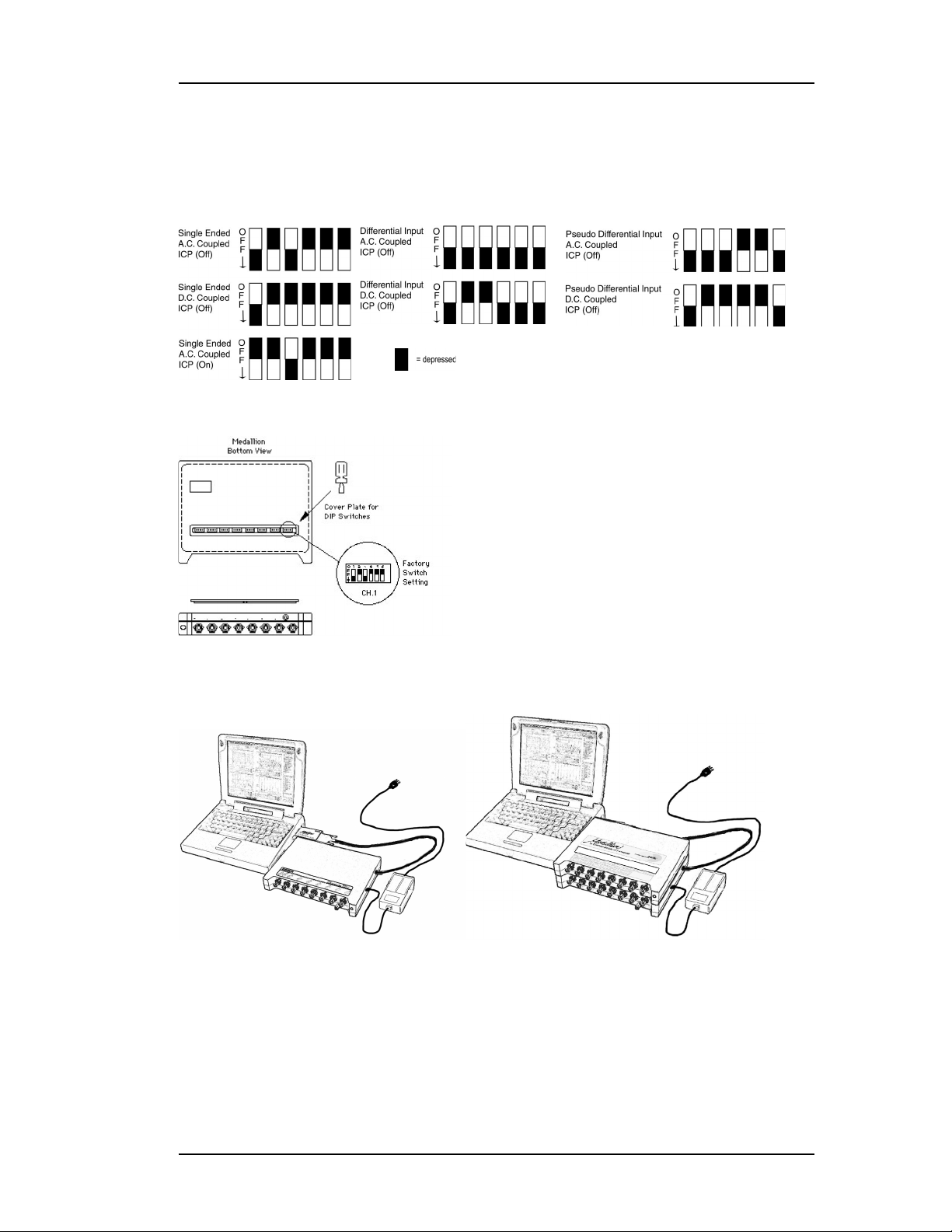
VERIFY SWITCH SETTINGS
The Medallion contains no relays. Switches control the input configuration.
These switches are set with rocker switches located under the access panel on
the bottom of the Medallion.
Improper settings CAN DAMAGE your equipment, and WILL PRODUCE
erroneous measurements.
CONNECT SIGNALS TO THE INPUT BNCS
Tip: Cap unused BNCs to reduce extraneous noise.
9
Page 10

eZ-Record Manual January 2001
VERIFYING MEDALLION’S OPERATING CONDITION
After the hardware is assembled, and the software is installed (See Getting
Started manual), you are ready to run your Medallion. Use this checklist to verify
that the Medallion hardware and software are operating properly .
Software Installed? See Software Installation in the Getting Started manual.
Hardware Switches Set? See Configuring the Medallion Front-End .
Hardware Connected? See Hardware Assembly .
eZ-Record Software running? On the Start menu select Programs, then
Zonic Medallion, and then eZ-Record. Your software opens to a Main
window where you can acquire/record new data, post-process existing data
either by playing back previously recorded data or recalling previously saved
functions.
If you are not using your Medallion analyzer, a message will appear that
hardware is not present. This is a reminder to you that new data can not be
acquired and that recorded data can not be processed with a trigger.
Signal Connected to Channel 1? Use Internal or External Signal Generator.
Signal Generator Turn ON? If using the Internal Signal Generator, press
Signal Generator button on the Task Bar in the Main window.
Medallion Acquiring Data? Click the Scope button. You should see a signal
with a 500 Hz Peak in the Plot Display window.
ORDER OF OPERA TION
1. Verify switch settings.
2. Connect signals to the input BNCs on the front of the Medallion.
3. Start the eZ-Record Software.
4. Configure the Medallion. On the Edit Menu select Medallion to open the
Medallion Configuration window. Review and edit the Medallion
configuration using the six tabs in the window.
5. If you need an output signal, click the Signal Generator button at the top of
the Main window.
6a. Recall previously captured data.
6b. Capture or record data. Click the SCOPE or Record button in the Task bar.
If you are setup for triggered acquisition, the analyzer status bar will change
from “Idle” to “A waiting T rigger .” When a trigger is recognized, the analyzer
status will change to “Triggered.” When a frame of data is captured, the
analyzer status will change to “Completed” and increment the Averages
status by one.
If the Averages status does not equal the number of averages requested in
the Analyzer Setup, the status will briefly change from “Idle” to “A waiting
Trigger.” If the Averages status does equal the number of averages
requested, the status will change to IDLE and the HALT button will change
to ACQUIRE. This indicates that one measurement has been captured.
7. Save your data. To save the function files, select Export on the File menu.
10
Page 11
January 2001 eZ-Record Manual
CHAPTER ONE - MENUS
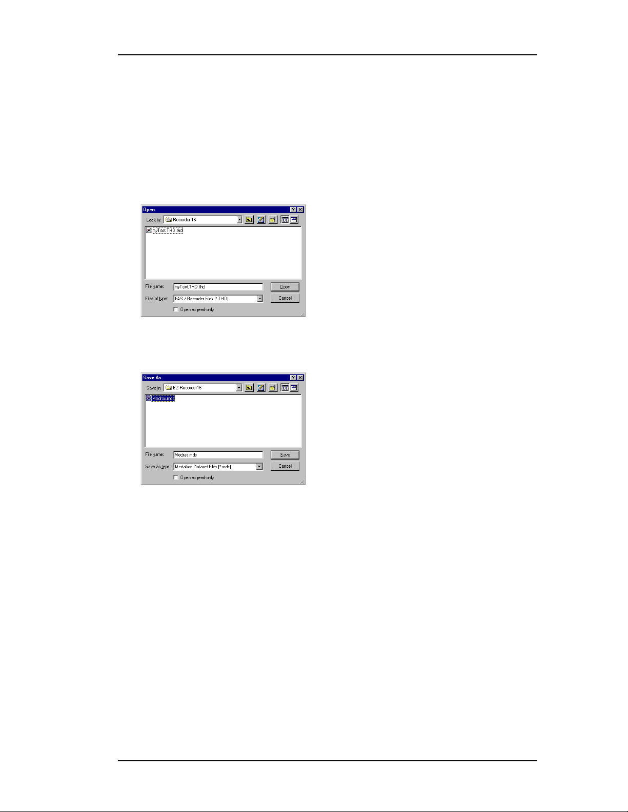
FILE MENU
File Menu selections provide the means for opening, saving, and exporting files;
in addition to printing plotted data. File formats are .thd (time history data) and
.mds (medallion data set).
PEN FILE
O
This menu item opens saved files. Use standard Windows conventions to find the
file of interest. Highlight the file name of interest and click the Open button.
SAVE DATA SET
This menu item saves the current function files and their display setup. The file
extension is .mds. T o export these files see the Export Menu.
The standard print window associated with your specific computer will open.
Select a printer and the number of copies needed before clicking OK.
Note: For printing purposes, if the background of the plot is black, it will be
changed to white.
EXIT
This menu item closes the eZ-Record application.
11
Page 12
eZ-Record Manual January 2001
EDIT MENU
Edit Menu selections provide the means make changes to the software
configuration.
EDALLION
M
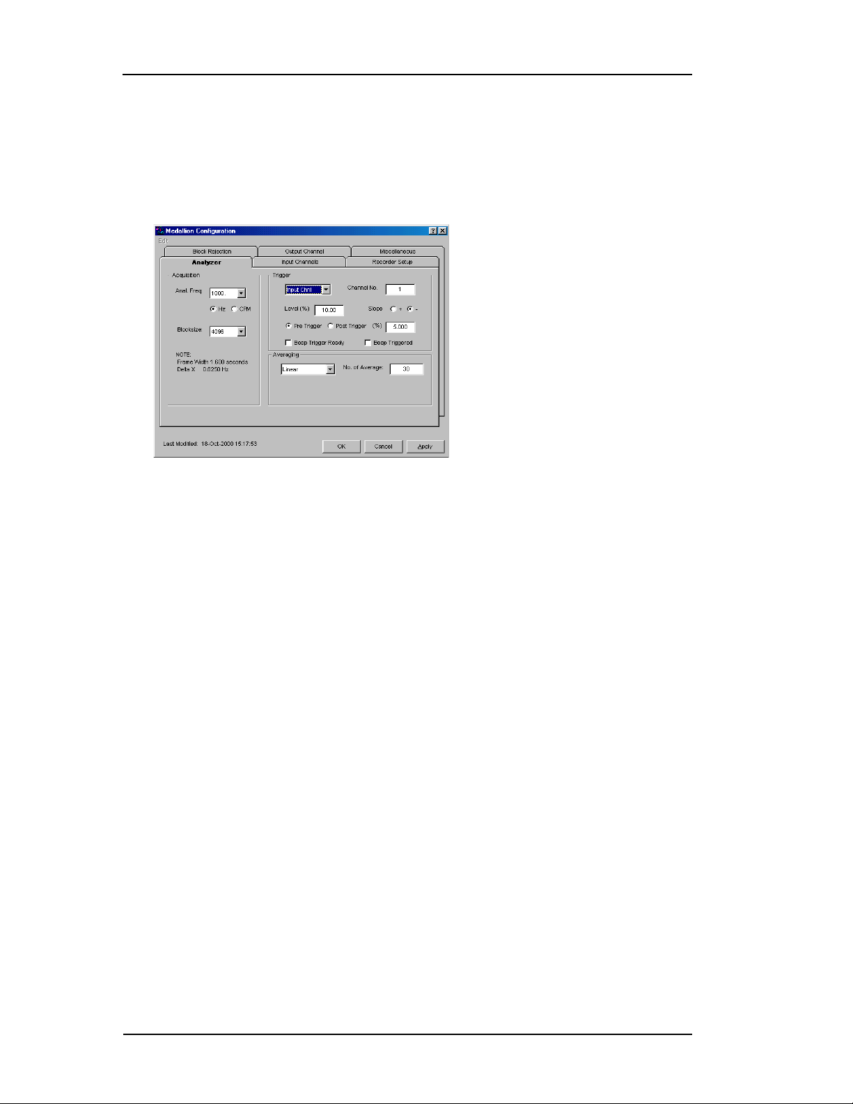
In the Main Menu select Edit and then select Medallion. The Medallion
Configuration window will open. This window has six (6) panels.
Analyzer Tab - Acquisition Panel
Analysis Frequency: Selections range from 10 to 20,000 for 8 channel analyzers
and 10 to 10,000 for 16 channel analyzers. The bandwidth measurement unit
for the X-axis is specified in Hertz (Hz) or Cycles Per Minute (CPM). Click to
place a bullet next to your preference.
Blocksize is the number of data points in a frame or block of data. Sizes range
from 128 to 16384. Make your selection in the popup menu.
As frame size increases, the resolution of the data increases, the time required
to acquire a block of data increases and the amount of space required to save
the data increases.
The rest of the information in this section is calculated using your
specifications.
Frame Width = Frame Size / (Bandwidth x 2.56)
Delta X = (Bandwidth x 2.56) / Frame Size
12
Page 13

January 2001 eZ-Record Manual
Analyzer Tab - Trigger Panel
Triggering is the method used by the analyzer to start capturing and
processing data. To capture continuous data, select Free Run. To capture
transient data, select Input Channel and specify the channel where the
analyzer should expect to “see” the signal.
For example, if you are using an impact hammer for modal analysis, the
hammer is attached to the specified input channel. For this type of test, you
may also want to average a set number of acquisitions before saving the data
(See Number of Averages). Y ou may also want the option to automatically or
manually reject measurements caused by double hammers and overloads.
(See Block Rejection.) (Also see: Hints for Trigger Setup and Double
Hammer Rejection.)
Trigger conditions are used by the analyzer to determine the trigger signal’s
attributes required to start data acquisition. Triggered acquisition is typically
used to capture a specific recurring event. Because the analyzer is always
capturing data, and storing it in the memory buffer , you can specify a pretrigger that tells the analyzer how much data you want captured before that
event occurs. This also insures that you get the full event and not just the
data that follows it. On the other hand, you may know that something is
occurring x amount of time after an event. In that case, you may want to set
up a post-trigger. A post-trigger tells the analyzer to look for an event, then
wait a specific amount of time and then start capturing data.
A trigger is specified by the signal level (as a percent of the Full Scale), the
signal’s location on a slope (ascending/positive; or descending/negative).
Other factors that determine what data is captured when a trigger condition
occurs are the amount of time (as a percentage of the frame/block of data)
associated with a pre- or post-trigger .
To understand the concept of Pre and Post Triggering you must remember
that when the green light on the front of the Medallion is glowing, it is
“seeing” data and sending that data to the DSP. If you have not clicked the
acquire button, this data is not processed. However, the DSP has 4 MB of
memory (memory buffer). It therefore has the capability to “remember” this
unprocessed data.
That said, lets look at trigger modes and what they mean.
13
Page 14

eZ-Record Manual January 2001
The pre-trigger mode includes data before the trigger event. When you specify a
pre-trigger, data in the memory buffer that precedes the trigger event is included
in the frame of captured data. The amount of data included is based on a percent
of the frame size.
A post trigger skips data immediately after the trigger event before it starts
capturing data. The amount of skipped data is based on a percent of the frame
size. This is specified in the Delay text field.
Free Run: Data acquisition and processing begin as soon as the Acquire
button is clicked.
Input Channel: Data acquisition and processing begin after the signal on the
specified channel reaches the defined trigger conditions.
Channel: This is the channel number where the analyzer will “look for” the
trigger signal.
Pre/Post Trigger: This is the amount of data, as a percent of the frame size,
that is captured before a trigger event (pre-trigger mode) or that is skipped
after a trigger event (post-trigger).
Neg/Pos: This is the (negative/decreasing or positive/increasing) slope of the
signal that defines a trigger condition. The signal must be on the defined
slope before it is considered a candidate for a trigger.
Trigger Level: This is as a percent of the Full Scale Voltage of the trigger
channel. The signal must pass through this level before it is considered a
candidate for a trigger. The slope of the signal must also meet defined trigger
slope condition before it is recognized as a trigger or trigger event.
Analyzer Tab - Averaging Panel
This is the type of averaging that will be calculated during data acquisition.
Averaging is one technique used to decrease the noise in a measurement.
Linear: All blocks of data are treated equally in terms of their effect on the
averaged result.
Exponential: Similar to linear averaging, Exponential requires a weighting factor
that either increases or decreases the effect of each new data block on the
resultant average.
Average Weight Factor: The Weighting Factor either increases or decreases
the effect of each new data block on the resultant average when
Exponential Averaging is used.
New Average = ((New Data) * A.W.F.) + (Old Average * (1-A.W.F))
Peak Hold: The resultant block of data is a collection of points that represent
the peak amplitude for each point in the block. With each new block of data,
the current data is compared with the new data on a point by point basis.
The highest amplitude for each point in the block is retained.
14
Page 15
January 2001 eZ-Record Manual
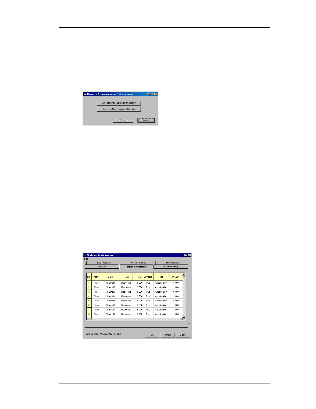
Linear (-): Also known as Negative Averaging; Linear (-) Averaging is a
technique used to identify the natural frequencies of in-service machines that
cannot be shut down for analysis. Linear (-) Averaging is a two step process.
First, a reference average is acquired. Second, a normal linear average is
acquired for each frame. The running average is subtracted from the
reference average and the result is displayed. The first time you attempt to
start data acquisition after you select Linear (-) averaging, the Negative
Averaging Setup/ Measurement window opens.
Time Sync: Time synchronous averaging uses a keyway, or a similar point of
reference, as a trigger. The blocksize is set to allow enough time for at least
one full revolution. This must be performed in Scope Mode.
Number of Averages: This specifies the condition for terminating a data
acquisition sample. After the number of averages (blocks/frames of data)
have been captured and averaged, the analyzer will automatically stop taking
new data. This sample can then be saved. If the number of averages is set to
zero, acquisition is continuous and must be halted by you.
Input Channels Tab
The Input Channel panel displays the current setup conditions of the input
channels on a channel-by-channel basis. Displays change as soon as they are
applied or okayed. Click on the Input Channels tab.
Note: When using the grid in this window, select a cell by clicking in it. You
many also highlight a range of cells by clicking on a second cell while
holding down the Shift key. A cell is selected (highlighted) when there is
a blue border around it.
No.: This column lists all the analyzer’s channels.
Active: When you start the analyzer, all input channels are active. For
channels you are not using, change the active status to FALSE. (Note: This
is optional.)
15
Page 16

eZ-Record Manual January 2001
To change the Active Status of a Channel, click in the cell for the channel of
interest and select True or False on the popup menu.
Label: This should be a meaningful name that you assign to the signal received
on a channel. The channel number is automatically assigned. Highlight a cell
before typing a label. When you press the Enter key, the value is accepted.
R T ype: There are two types of Channels: Response or Reference. All
channels are initialized as response channels. If you are using a force
channel highlight that channels R Type cell, select reference on the
popup menu and press Enter.
FSV: F(ull) S(cale) V(oltage): The value in this field sets the Full Scale value in
Volts. The acceptable range of values is 0.0019 V to 25 V.
EU Mode: E(ngineering) U(nits): Select True or False.
I Type: This is the type of instrument attached to the channel. Menu selections
include: Acceleration, Velocity, Displacement, Force, Pressure, Stress, Strain,
and General.
mV/EU: This is the scaling factor of millivolts to your Engineering Units.
dB EU Ref: dB EU Reference is applied to displayed data when the Y-axis scale
is set to dB. This is valid only for frequency domain data.
The formula for dB display for Unaveraged Spectrum, Averaged Spectrum,
and FRF is:
dB = 20 log (x/dBEUref)
The formula for dB display for Autospectrum, Cross Spectrum, and PSD is:
dB =10log[x/((dBEUref)^2)]
See also dB Reference (Volt) in the Miscellaneous T ab.
Units: Enter the measurement units you will be using.
Location: This is a simple numbering system. The channel number is the
default value for location. However, you can highlight a cell and type a
different location number. When you press the Enter key, the value is
accepted.
Coord: This is the axial direction of the transducer connected to the channel.
Make your selection on the popup menu. Note: The coordinate system is
selected in the Miscellaneous panel.
16
Page 17

January 2001 eZ-Record Manual
Recorder Setup Tab
Active Channels: This is the number of contiguous channels (starting with
channel 1) being used.
Recording Duration/Trigger: The amount of time (in seconds) or data blocks
(number) to be included in the recorded file.
Trigger Delay: This value is used with Pre Trigger and Post Trigger. With Pre
Trigger, Trigger Delay is the amount of time or the percentage of the data
block prior to the Trigger when data acquisition is captured. With Post
Trigger, Trigger Delay is the amount of time or the percentage of the data
block that is skipped from the time of the trigger to the start of data
acquisition. With Post Trigger
Comments: Your comments about this file. For example, they may include the
environmental condition at the time of the recording, the phase of a project,
or a problem that you are investigating.
Block Rejection Tab
This panel is only active when Measure on the Task menu is selected.
Because each strike of an impact hammer may not have the desired results, Block
Rejection allows you to reject a block of data that is the result of a double strike,
an over or under load, or simply because it “doesn’t look right.” Auto block
rejection looks at the acceptable parameters for a block and automatically rejects
blocks that do not meet those parameters. Manual rejection allows you to look at
each block of data and allows you to determine if it should be rejected.
17
Page 18

eZ-Record Manual January 2001
Block Rejection Tab - Reject Panel
There are three block rejection modes: Double Hammer protects measurements
against double hammering: Overload protects the measurement by automatically
rejecting overloaded data, and Manual allows you to inspect a measurement and
optionally reject it for any reason. You can select any or all of the rejection
modes. (See also: Hints for T rigger Setup and Double Hammer Rejection)
Double Hammer: A double hammer occurs when a signal goes outside of the
acceptable range that is set up in the Hammer Rejection section. Click in the
Double Hammer box to turn the Double Hammer option ON and OFF. When
the box is checked, the option is ON.
Overload: An overload is any input signal that reaches or exceeds the specified
input Full Scale Voltage range. Click in the Overload box to turn the Overload
Rejection option ON and OFF. When the box is checked, the option is ON.
Manual: This option allows you to review each block of data before acquiring
the next block. When manual rejection is selected, a “Reject?” button is
activated in the main window. At the end of each average, if you want to
reject that measurement, click on the “Reject?” button. The analyzer will then
reject the current frame of data. The data and average counter will go back to
the previous measurement. Click in the Manual box to turn the Manual
option ON and OFF. When the box is checked, the option is ON.
Block Rejection Tab - Hammer Rejection Panel
In this panel you define the acceptable range for a hammer signal. Any signal
outside of this range is detected as a double hammer . The acceptable range looks
like the intersection of two roads. The signal must occur at the intersection.
X-axis Limits (% of blocksize): The x-axis Limits set the intersection at which
the impact must occur on the “road.”
Y-axis Limits (% of F(ull) S(cale): The y-axis Limits set the “road or lane
width” that extents across the x-axis.
Hints for Trigger Setup and Double Hammer Rejection
There are three major interrelated components to consider when setting up the
analyzer for double-hammer rejection.
1. Trigger Mode and Delay
2. Force Window
3. Double Hammer Region.
A trigger is used to ensure time synchronous measurements across all the active
channels. Pre-trigger states that the amount of data (specified by the delay) is
captured before a trigger event and prefixed to the data following the trigger
event. Post-trigger states that the amount of data (specified by the delay) is
discarded after the trigger event before capturing a block of data.
Double hammer reject is only meaningful with the pre-trigger specified. Double
hammer rejection protects the measurement from a bad hammering.
It is desirable to set the pre-trigger to fall within the hammer region, since it is a
common practice to set the trigger channel to an impact channel.
18
Page 19

January 2001 eZ-Record Manual
Example
Set a Pre - Trigger with a 10% Delay.
Set a Rectangular Force Window with a Start Edge of 9% and an End Edge of
15%.
So far we have said we want to start looking for a trigger event in the data
somewhere after 10% of the block and before 15% of the block. When impact
testing we also want to make sure that a double hammer does not occur . Through
trial and error we may start by setting the Double Hammer range at 12% and 14%,
or 11% and 13% of the block. Typically this range is fine tuned using sample
acquisitions prior to starting a real test.
Output Channel Tab
The Internal Signal Generator is set up in the Output Channel panel. Select an
output waveform (Sine, Random, or Sine+Random) on the popup menu.
Sine Amplitude: The maximum amplitude range is 1.4 volts zero-to-peak. Type
a value, in Volts, and press the “Enter” key.
Sine Frequency: This is the frequency, in Hz, for a Sine waveform. Type a
value (2,000 maximum) in Hz and press the “Enter” key.
Random Amplitude: This is the amplitude variance for the Random output
signal. The maximum value is 1.4 volts zero-to-peak. Type a value, in Volts,
and press the “Enter” key.
19
Page 20

eZ-Record Manual January 2001
Miscellaneous Tab - FFT Window (Response) Panel
The FFT (Response) window is a time-domain weighting window . A response
window is usually applied to data to reduce FFT leakage errors. FFT theory
assumes that the signal being analyzed is periodic in the data acquisition block.
When this is not the case, energy from a signal at a specified frequency can leak
into nearby spectral bins causing spectral amplitude inaccuracies. Applying a
windowing function controls, but doesn’t completely eliminate, the error by
multiplying each data frame by a suitable time-domain weighting window . This
calculation reduces the amplitude/magnitude of the data near the ends of each
data frame prior to performing the FFT and forces the data to be nearly periodic in
the window , thus reducing leakage errors. Response window options are:
None: No weighting window is applied.
Hanning: The Hanning window is typically used to analyze continuous
signals. It offers a reasonable trade-off of frequency accuracy versus
amplitude accuracy .
FlatTop: Compared to the very similar 4-term “Max Flat Top,” this window also
has a very low peak amplitude error, and its frequency resolution is
somewhat better . Its side lobes are considerably higher. Its effective noise
bandwidth is still almost twice that of the Hanning window , therefore this
window is used mainly to measure accurate peak amplitudes of discrete
spectral components that are known to be separated by at least several
spectral lines.
Blackman-Harris: This window function was designed to provide the
minimum side lobe level of any three-term window . Compared with the very
similar Hanning window , it has a slightly wider main lobe but much better
dynamic range. This window has the smallest 60 dB bandwidth of any
window listed. The Blackman-Harris window may be preferred over the
Hanning for measurements requiring better dynamic range.
Exponential: An exponential weighting window is equal to 1.0 at the beginning
of the block and decays exponentially to a smaller value at the end of the
block. Exponential is used only with transient data that is captured with
pre-trigger to assure that the initial values in all data channels are very
20
Page 21

January 2001 eZ-Record Manual
close to zero. Exponential can be used with all transient excitation methods
in order to force the signals to decay close to zero, (See Response Decay
Percent,) even if the block length is not sufficient to capture all of the
naturally occurring response. If the data decays naturally to a low
amplitude within the block, so that leakage is not significant, exponential
windowing can improve the signal-to-noise ratio by giving reduced weight
to the very low-amplitude data at the end of the block.
Response Decay Percent: The Response Decay Percent is used when an
Exponential Window is applied to the Response Channel. It is the rate of
decay from the first to the last block value.
Miscellaneous Tab - FFT Window (Reference) Panel
The FFT Reference Window is applied to the output (force) of a transducer to
avoid collecting extraneous signals caused by an excitation device, such as an
impulse hammer .
When Rectangular is selected, specify the Start and End of the rectangle as a
percentage of the Frame Period.
When Cosine Taper is selected, specify the Start, End, and Taper of the Cosine
Taper as a percentage of the Frame Period.
Start: This is the percent of the Frame Period at which the Rectangular and
Cosine Taper Windowing functions start.
Stop: This is the percent of the Frame Period at which the Rectangular and
Cosine Tape Windowing functions stop.
Edge: This is the percent of the Frame Period during which the Cosine Taper
Windowing function tapers up and down.
Miscellaneous Tab - Octave Panel
Weighting: No weighting, A B or C Weighting
Filter: Analog or Digital
Miscellaneous Tab -
Differentiation/Integration: g’s-ips-mils, g’s-ips-in, g’s-fps-ft, ips^2-ips-in,
ips^2-ips-ft, fps^2-fps-ft, g’s-mmps-micr, g’s-mmps-mm, g’s-cmps-cm,
mmps^2-mmps-mm, cmps^2-cmps-cm, mps^2-mps-m
Miscellaneous Tab - Low Frequency Cutoff Panel
Low frequency cutoff is used to remove the low frequency effects of integration.
All data point below the value specified are set to zero.
Single: Enter a value for the cutoff amount for single integration.
Double (Hz): Enter a value for the cutoff amount for double integration .
Integration Panel
21
Page 22

eZ-Record Manual January 2001
Miscellaneous Tab - Modal Coordinate System Panel
There are three coordinate systems - Rectangular, Spherical, and Cylindrical.
Make your selection on the menu.
Auto Bank Switch: If the Auto Bank Switch checkbox is checked, the bank is
automatically incremented or decremented each time the Export button is
pressed at the end of an acquisition.
A Bank is a set of response channels. You can have the analyzer increment
your banks automatically after each measurement, or you can manually
increment the banks. The number of active channels is used as the skip
factor for bank switching
Skip Ref Channels: If the checkbox is checked, then the number of locations
skipped is the same as the number of Response Channels. Click to place an
X in the check box.
Skip Res Channels: If the checkbox is checked, the only channel skipped is
the Reference Channel. The Response channels DO NOT SKIP.
dB Reference (Volt): dB EU Reference (Volt) is applied to displayed data (all
channels) when the Y-axis scale is set to dB. This is valid only for frequency
domain data.
See also: dB EU Ref in the Input Channels Tab.
PLAYBACK SETUP
After you open a recorded file to be played back, you have the option to change
the blocksize and frequency range, for viewing purposes only.
Frequency Range selections are from 31.25 to 1000 Hz.
Blocksize selections are 4096, 8192, and 16,384.
22
Page 23

January 2001 eZ-Record Manual
WINDOW COLORS
Plot window defaults:
Frame Border = Grey
Plot Background = Black
Grid Lines = Grey
Cursor = White
There are four cursors.
1: Single cursor
2: Second cursor of band cursors
3: Peak Search cursor
4: Data List
1. To change a display characteristic’s color, click on the appropriate button,
to open the Color Palette.
2 . Click on a color square, and click OK.
3. Repeat for each color you want to change.
4 . When finished, click OK in the Plot W indow Colors window .
23
Page 24

eZ-Record Manual January 2001
PREFERENCES
The Preferences window provides a means for you to set some defaults for your
acquisitions.
T race Colors - Click on a channel’ s color chip to open a color palette. Pick a
new color and click ok.
Labels Colors - These are the on-plot text labels you can add to notate your
data plots. Click on a color chip to open a color palette. Pick a new color
and click ok.
Monitor Window - Sets how the monitor window displays information.
Cursor Movement Control - Sets the cursor’s action. Pick means any mouse
click on the plot will move the cursor to the location of the click. Drag
means you must click on and then drag the cursor to a new location.
Peak Search - Sets the minimum data searched. You can set this value
somewhere above the extraneous noise level. Peak averages are evaluated
by first finding a peak and then averaging the specified number of spectral
lines on either side of the peak. The default is 3.
Band Bin: This number specifies the number of data bins used for peak
searching. For example, “3” means that the left three and the right three
adjacent data are compared for around a peak.
Sort By - Specifies the order of the data in the peak search table.
Octave band type: When this box is checked solid color bars are used in Octave
plots. When this box is unchecked, the bars are “hollow,” only the outline
of each bar is displayed.
24
Page 25

January 2001 eZ-Record Manual
TASK BAR
Playback Controls
The Playback option appears on your main screen as a series of icons that
resemble and work like a VCR. The left arrows “backward playing” and the
right arrows “play .” The arrows with vertical lines “backward playing” and
“play” one frame at a time. The square stops play . Select Playback/Review
on the Task Menu to activate the Playback Controls
Record Button
This button is used to start recording. Select Measurement on the Task
Menu to activate the Record Button.
Scope Button
This button is used to start data acquisition. If averaging is being performed,
it changes to ACQUIRE after all measurements and averaging is complete.
Select Measurement on the Task Menu to activate the Scope button.
Signal Generator On/Off Button
T oggles the Signal Generator between on and off. The Signal Generator
button is only active when hardware is present.
Cursor Lock
The Cursor Padlock button toggles the cursor between a lock position and
free movement. If the Padlock is closed, cursors are synchronized in multiple
windows when they are of the same time domain, same frequency domain, or
same octave band data.
Export Button
Click this button to export data. Prior to using this button you must first set
up the condition for Exporting data in the Save Export Function Data window
access via the Export Menu.
Acquisition Status Panel
This icon indicates the acquisition status of the analyzer.
Waiting Trigger: A trigger has not been recognized, since the Acquire button
was clicked.
Triggered: Analyzer is capturing and processing data based on the setup
conditions.
Completed: Analyzer has finished processing the frame of data. The “Averages
Count” increments by 1 at this time.
Analyzer Status Message Area
The analyzer status is displayed in this area. Messages you may see are
Armed, W aiting Trigger , T riggered, Completed, Stopped, Double Hammer
Rejected, Overload Rejected, Exporting Function Data.
25
Page 26

eZ-Record Manual January 2001
Playback Display Bar
The sliding bar indicates the relative location of the displayed data. The
record number and the number of records in the file are listed to the right.
The slider can be used to quickly locate a specific record.
Channels
Each of these boxes represents an analyzer channel.Drag a channel to the
plot area to have its data displayed. That channel’s data is plotted in a
distinct color and a color-coded channel button is displayed to the right of
the plot. Reference channels ar bold and italic. The underlined channel is the
current reference channel. Use the right mouse button to select current
reference channel. Reference channels are specified in the Medallion
Configuration accessed via the Edit Menu.
Averaging Status 5/10
The Averaging Status displays the current number of the averages for the
current record and the total number of averages to be collected.
i.e. 5/10 means that so far 5 averages have been been performed and there are
a total of 10 averages to be performed.
26
Page 27

January 2001 eZ-Record Manual
TASK MENU
MEASUREMENT
Select Measurement to activate the Record and Scope buttons on the Task bar.
PLAYBACK / REVIEW
Select Playback/Review to activate the Playback Controls on the Task bar.
CALIBRATION
Transducer calibration may be performed when a calibration signal of a
known level or RMS content is available. The known signal can be applied to
the transducer connected to an input channel. Two types of calibrators are
commonly used; 1) desktop calibrators for transducers such as
accelerometers, strain gauge, etc. and 2) piston phones for microphone
calibration. Linear engineering units are commonly used for the former type
and dB engineering units for the latter type.
After calibration is finished, the measured voltage(s) for the selected
channel(s) is(are) displayed in the Volts field and used in the calculation of
EU/Volt.
Note: When using one calibrator, you can only calibrate one channel at a time.
No.: This column lists the channels of the Medallion Data Acquisition Module.
Active: True, False. Select True for each channel to be calibrated. Select False
for each channel not to be calibrated. Note: This is independent of
selections in the Input Channel Setup window.
Type: Peak, RMS. Highlight a cell, or range of cells, in the grid before selecting a
Calibration Type on the popup menu.
Peak uses the peak amplitude of the spectrum around the specified
frequency of the calibration signal. The measured peak voltage is entered
into the “Volt” field and further used to determine “EU/Volt”. Please see
the section, “Performing Calibration”, for examples. It searches total seven
spectral lines for the peak; three lines on either side of the specified
calibration frequency.
RMS uses a compensated overall level calculation to determine the RMS
level of the calibration signal, as specified in the Units field. The overall
calculation compensates for the effect of low frequency noise in the
calibration signal by ignoring the first four spectral lines.
27
Page 28

eZ-Record Manual January 2001
Unit: dB, EU.
dB is applied to displayed data when the Y-axis scale is set to dB. This is
valid only for frequency domain data.
The formula for dB display for A veraged Spectrum is:
dB = 20 log (x/dBEUref)
EU/Volt is determined as follows:
EU/Volt = Units / Volts / Trans. Gain, where Units is linear.
Highlight a cell, or cells, in the grid before typing a value in the data entry
box. Then press the Enter key to accept the value. All other fields linked to
this value are updated when the value is accepted.
Amplitude: The amplitude of the calibrator.
Gain: This is an auxiliary scaling factor. It is typically used to compensate for
the signal gain of external signal conditioning such as a charge amplifier with
gain.
mV/EU: Units and Volts: These fields can be either entered by you or
measured by calibration. The separate Units and Volts fields are provided for
easy EU/Volt specification and calibration. Volts is used in conjunction with
the Units to determine the EU/Volt.
Trans. Gain is used as auxiliary scaling to compensate for the transducer gain.
Date: The date and time of the last calibration is recorded in this column. If
any channel value changes (even if the original number is restored), the
calibration date and time are removed for that channel.
Calibration Signal Frequency: Enter the frequency of the calibrator. The
frequency range is set to 2.56 times the frequency of the calibrator.
When you press the Calibration button, the Signal Range is calculated and
displayed to the left of the Calibration Status bar.
Start button: Clicking this button will perform calibration for all the selected
channels. The measured voltage will be displayed in the “Volts” field that is
used for the determination of “EU/Volt”.
28
Page 29

January 2001 eZ-Record Manual
CALIBRATION PROCEDURE
Example
Accelerometer type - Piezotronics 303A03
Calibrator - Piezotronics 394B05 - 1.02 G (RMS) at 80Hz
Unit of acceleration - in/sec^2
Note:
1.02 G RMS is equivalent to 1.4423 G PEAK (=1.414*1.02) and 1G=386.089 in/
sec^2. Thus 1.02 G RMS is equal to 556.8484 in/sec^2. This is a linear type. Thus
select “Linear” calibration unit.
1. Attach the accelerometer to the calibrator (signal source). Connect the other
end of the accelerometer cable to the channel you want to calibrate (i.e.
channel 1).
2. Set an appropriate bandwidth in the Analyzer Setup window (i.e. 200 Hz).
Select a response window other than exponential and no force window. If you
are not providing a trigger signal choose free run Start Mode.
3. Set the FSV into a proper range (i.e. 32.4 mV) in the Input Setup window and
click the Apply button.
4. Open the Calibration Window.
5. Select True for the channel(s) to be calibrated.
6. Enter the scale (i.e. 556.843) in the Units field.
7. Enter the calibrator frequency. (i.e. 80 Hz).
8. Click the Start Button to begin calibration.
29
Page 30

eZ-Record Manual January 2001
AUTORANGE
Autoranging is a procedure that automatically sets the input full scale voltage
(FSV) range for input channels. FSV is set by measuring a representative sample
of real-time data. It is performed only on active channels.
Autoranging works best if you supply the same type live data you will be
capturing during data acquisition. If you are performing an averaged count, the
count will automatically reset to one. If your capture mode is triggered, you will
have to supply a trigger . If your capture mode is Free Run, the autoranging
process starts automatically.
When the Auto Range window opens, the number at the bottom of each column
is the Current FSV are the same values that were entered in the Vpeak column in
the Channel Setup window . These values are immediately replaced when the
Auto ranging process begins.
For example, if in the Autorange Setup window you specify Maximum FSV as 80,
Minimum FSV as 45, Increasing factor as 1.333 and Decreasing factor as 1.333 the
following will occur.
For the first iteration, if the peak value of the data block is greater than 0.8 times
the FSV set in the Channel Setup window , or less than 0.45 times the FSV, then the
Current FSV fields are changed to 1.333 times the peak found in the acquisition.
For the rest of the iterations, if the instantaneous peak value is greater than 80
percent of the Current FSV, the Current FSV is recalculated to 1.333 times the peak
found in the acquisition. This process will continue for 100 iterations, or you may
click the OK button when you are satisfied with the input range.
If the Capture Mode is Input Channel (Trigger Mode), the Auto Range process
waits for a trigger .
Monitoring the Instantaneous Signal Level
The instantaneous peak value is graphically displayed in the vertical bars.
Yellow= signal range is from 0 to the minimum Full Scale voltage set in the
Autorange Setup window.
Gre en = signal range is from the minimum to the maximum of the Full Scale
voltage set in the Autorange Setup window.
Red = signal range is over the maximum of the Full Scale voltage set in the
Autorange Setup window.
30
Page 31

January 2001 eZ-Record Manual
Setup Autoranging Parameters
1. On the Task Menu select Autorange to open the Auto Range window.
2. Select the Setup Menu to open the Autorange Setup window. Use this
window when you want to change the default values described above.
3. Type values for the Minimum and Maximum FSV; and for the Increasing
and Decreasing Factors.
EXPORT MENU
EXPORT TIME HISTORY DATA
This menu item is for exporting Recorded Files.
1. Select the type of file you want. Binary (THD) Time History or ASCII (TXT).
2. Type the directory path and file name for the recorded file. The correct file
extension will be appended to the file name when the OK button is clicked.
3. Optionally, add comments about the file in the data entry area provided.
4. Specify the channels of interest. Click to place a checkmark in the channel
box for each of the channels you want to export.
5. Specify the First (Starting) and Last (Ending) records (blocks) that you want
saved; and click the OK button.
31
Page 32

eZ-Record Manual January 2001
SETUP EXPORT FUNCTION DATA
This menu item is for exporting function files.
1 . T ype the directory path and file name for the function file. The correct file
extension will be appended to the file name when the OK button is clicked.
2 . Select the type of file you want. Universal ASCII T ype 58 or Universal
Binary T ype 58.
3 . Select Automatic Save after Averaging to have records automatically
appended to the specified file.
4 . Specify either All Ch Pairs or Displayed Ch and Functions.
All Ch Pairs exports all the data for all the channels pairs so that all
functions can be retrieved if desired
Displayed Ch and Functions exports only the data for the displayed
functions.
5 . Click to place a checkmark by the functions to be saved; and click the OK
button.
32
Page 33

January 2001 eZ-Record Manual
WINDOW MENU
ADD FUNCTION VIEW
This menu selection opens an addition plot window.
ADD STRIP CHART
This menu selection opens a strip chart plot window.
DELETE WINDOW
Click on the window of interest to make it the “focus” window . Then select this
menu option to delete the window .
MODAL LOCA TIONS WINDOW
This window displays the current modal locations.
Clicking on the Up or Down buttons increments or decrements the locations
based on the bank setup criteria set in the Medallion Configuration –
Miscellaneous T ab. For example if you have Skip Response channels checked,
each time you click up or down, the only the location of the reference channel will
increment or decrement. However if you have Skip Reference channels checked,
each time you click up or down, the locations will change by the number of
response only channels you have defined. If you have neither of the above
checked, the locations will change by the number of active channels.
33
Page 34

eZ-Record Manual January 2001
CHANNEL MONITOR
Channels can be monitored in Volt or % of FSV mode.
Blue: The maximum time data value during the whole acquisition period.
Green: The current maximum time data value.
The Stop button on the Task bar resets the value of the blue bar.
CASCADE
When you have multiple plot windows open, this menu selection arranges them
on you screen as shown.
TILE VERTICALL Y
When you have multiple plot windows open, this menu selection arranges them
on you screen as shown.
34
Page 35

January 2001 eZ-Record Manual
TILE HORIZONTALLY
When you have multiple plot windows open; this menu selection arranges them
on your screen as shown.
PLOT DISPLAY WINDOW
The plot window is very interactive. Some activities are performed directly on the
plot, and clicking the right button on our mouse accesses many other options.
Change “focus window”
“Focus” window: When multiple plot windows are open one is always the
“focus window. ” In the below example, the top window is the “focus
window. ” It is the window with the dark blue border at the top. In the other
two windows, the top border is gray (dimmed).
To change the “focus window,” click on the top or right side border of the
window of interest.
35
Page 36

eZ-Record Manual January 2001
Change “focus plot”
“Focus” plot: When multiple plot windows are open, a plot other than the one
in the “focus” window can be the “focus plot.” You would typically do this
when you want to change a plot’s characteristics.
To change the “focus plot,” click in the plotted area of the window of
interest.
Change Plot Display Characteristics
To change a plot’s display characteristics; it must be the “focus plot.” Then,
you can either use the mouse or key commands to make changes.
Open Plot Display Characteristics Menu: Press “D” or right click with the
cursor hovering over the plotted data.
Use the down arrow key to highlight a menu option, then press “Enter”.
Note that in some cases you can press the first letter of an option to open its
sub menu. (i.e. “S” will open he Scale Type submenu.)
Add Channel to Plot
Using your mouse, click and drag a channel box (above the plot) to the plot
area.
Remove Channel from Plot
Using your mouse, click and drag a channel box (right of the plot) to the plot
area.
36
Page 37

January 2001 eZ-Record Manual
Display Functions
Open Function Menu: Right click on the plot.
Using Key Commands: Press “D” + “F”. Use the arrow keys to highlight your
selection and press “Enter”. Note that in some cases you can press the first
letter of an option to select it
The data type determines the functions available for display.
Time: A single-channel display function. Displays a time domain waveform of
filtered, sampled data scaled in either Volts or EUs.
Spectrum: A dual-channel display function. Displays averaged linear spectrum
computed as the square root of the averaged autospectrum. This function is
calibrated in peak engineering units (EU).
Auto Spec: A single-channel display function. Displays the square of the
magnitude of the complex (one-side) Fourier spectrum of x(t). Autospectra
are calibrated so that if A is the peak amplitude of a sinusoidal signal x(t),
then the autospectrum has the value A
2
at the sinusoidal frequency.
PSD: A single-channel display function. It is the Fourier Transform of the
Autocorrelation function. This normalization should be used with
continuous random signals.
Coherence: A dual-channel display function. At each frequency, the
coherence is a value between 0.0 and 1.0, which indicates the degree of
consistent linear relationship between two signals during the averaging
process. A value of less than one indicates that phase cancellation occurred
during cross-spectrum averaging, which may be due to uncorrelated noise on
one or both signals or to a nonlinear relationship between signals.
FRF: A dual-channel function for the single-input, single-output (SISO)
frequency response function between two specified input channels. FRF is
the averaged cross-spectrum divided by the averaged autospectrum of the
input (the second named channel).
Cross: A dual-channel display function in the frequency domain. It is equal to
the product of the complex Fourier spectrum of y(t) (the numerator or first
named channel) times the complex conjugate of the Fourier spectrum of x(t)
(the denominator or second named channel). The special case y=x yields the
autospectrum. Averaging of these functions (frequency-domain averaging)
forms the basic foundation on which virtually all other multichannel,
37
Page 38

eZ-Record Manual January 2001
frequency-domain analysis is built. The cross spectrum is calibrated in units
of (peak EUy) (peak EUx).
Octave: Many sounds, including audible noise for a transmission line, are
broad band, having components that are continuously distributed over a
range of frequencies. The spectrum of such a sound can be approximated in
terms of a series of octave band or one-third octave band pressure levels. A
band is designated by its center frequency, f
, which is the geometric mean of
0
the upper and lower frequencies of the band. (See ANSI/ASC S1.6-1984.
Activates the Octave Type menu. Select the desired Octave Type on the
Octave Type menu.
Transfer: Activates the Transfer Type menu option. Select the desired
Transfer Type on the Transfer Type menu.
Unaveraged Spectrum: A display function of the magnitude of instantaneous
unaveraged spectrum.
Averaged Time: A single-channel display function. Displays a time domain
waveform of filtered, averaged, sampled data scaled in either Volts or EUs.
Reference Spectrum minus Current Spectrum: Displays the difference
between the Reference Spectrum and the Current Spectrum when
Linear (-), Negative Averaging, is specified.
Windowed Time: Applies to the FFT Response window specified in the
Miscellaneous Tab of the Medallion Configuration window to time data.
38
Page 39

January 2001 eZ-Record Manual
COMPLEX DISPLAYS
Open Complex T ype Menu: Press “D” + “C” + “Enter”.
Use the down arrow key to highlight your selection and press “Enter”.
Options on the Complex Display menu are only available when a function
with complex data is displayed. The following options are available.
Magnitude: Plots only the magnitude of real or complex data.
Phase: Plots only the phase of complex data.
Real: Plots only the Real numbered data.
Imaginary: Plots only the imaginary numbered data.
Magnitude + Phase: Plots both Magnitude and Phase data.
Real + Imaginary: Plots both Real and Imaginarily data.
Nyquist: A Nyquist plot is another way to display real and imaginary data.
The real numbered data is plotted on the X-axis and the imaginary numbered
data is plotted on the Y-axis with consecutive points joined by line segments.
From basic vibration theory, a Nyquist plot of a mobility function should
trace out a circle (counter-clockwise) as the frequency is increased through
an isolated structural resonance.
TRANSFER TYPE
Open Transfer Type Menu: Press “D” + “T”.
Use the down arrow key to highlight your selection and press “Enter”.
These functions are calculated by dividing the cross spectrum of the channel
pair by the auto spectrum of the reference (force) channel.
· Inertance (acceleration/force)
· Mobility (velocity/force)
· Receptance or Compliance (displacement/force)
These reciprocal functions are derived from the first three by taking the
inverse of the magnitude reflecting the phase about the zero degree line (-1*
phase angle).
· Apparent Mass (force/acceleration)
· Impedance (force/velocity)
· Dynamic Stiffness (force/displacement)
39
Page 40

eZ-Record Manual January 2001
Note: Transfer function displays assume the reference channel is a force
channel. You MUST define the response channels to be the correct type of data
(acceleration, velocity, or displacement) that you are acquiring. Define these in
the data type column of the Calibration window. This allows the data to be
integrated or differentiated correctly to derive the desired transfer function.
OCTAVE TYPE
Many sounds, including audible noise for a transmission line, are broad band,
having components that are continuously distributed over a range of frequencies.
The spectrum of such a sound can be approximated in terms of a series of octave
band or one-third octave band pressure levels. A band is designated by its
center frequency , f
frequencies of the band. (See ANSI/ASC S1.6-1984.)
Open Octave Menu: Press “D” + “O”.
Use the down arrow key to highlight your selection and press “Enter”.
Full: An octave band extends from a lower frequency, f02 to twice the lower
frequency ( 2f0).
Third: A one-third octave band extends from a lower frequency ( f0/ 2) to
3 2 times the lower frequency (62 f0). The Octave (one-third octave)
band sound-pressure level is the integrated sound-pressure level of all
spectral components in the specified octave or one-third octave band.
, which is the geometric mean of the upper and lower
0
INTEGRA TION/DIFFERENTIATION
Open Int/Diff Menu: Press “D” + “I”.
Use the down arrow key to highlight your selection and press “Enter”.
This is for display purpose only and does not modify the data.
Differentiation/Integration is only active when frequency domain data is
displayed. Select single or double integration, single or double differentiation
or none. Make your selection on the popup menu.
Differentiation and Integration are calculated by dividing each element of the
function by (jw)^n, where j is the square root of -1; w is the product of 2 pi
times the frequency of the block element; and n is an integer from +2 to -2.
n = 2 is double integration
n = 1 is single integration
n = 0 has not effect
n = -1 is single differentiation
40
n = -2 is double differentiation.
Page 41

January 2001 eZ-Record Manual
If the signal is acceleration, then single integration (Int1) results in velocity,
and double integration (Int2) results in displacement. If the signal is
displacement, then single differentiation (Diff1) results in velocity, and
double differentiation (Diff2) results in acceleration.
Note:
Engineering Units change if instrument type is Acceleration and double
integration is selected.
SCALE TYPE
Open Scale Type Menu: Press “D” + “S”. Use the down-arrow key to highlight
your selection and press “Enter”.
RMS: (Root Mean Square): The square root of the average of the square of the
value of the function taken throughout one period.
Area (from Zero) under the peak.
Peak: Zero to Peak
Pk-Pk Peak to Peak
Absolute value from Zero
to Positive Peak
Absolute value from
Negative Peak to Positive Peak
41
Page 42

eZ-Record Manual January 2001
COPY
Open Copy Menu: Press “D” + “C” use the down arrow key to highlight Copy
and Press “Enter”. Use the down arrow key to highlight your selection and
press “Enter.”
You can copy the plotted data, the plot window, or the screen and then paste
them into other applications. For example, plotted data can be copied into
Notepad, Word, or Excel for use in reports or in the case of Excel further
calculations.
The plot window and full screen can be copied and then pasted into any
application that accepts graphics, such as MSPaint or Word.
CURSOR
Open Cursor Menu: Press “D” + “C.”
Use the down-arrow key to highlight Cursor and press “Enter”. Then use
the arrow key to highlight your selection and press “Enter .”
When Single Cursor is selected, a cursor appears at the far left of the plot
and cursor controls and cursor information are added below the plot. Click
on the plot where you want the cursor. To fine-tune the cursor location, use
the right and left arrows at the bottom. Use the X and Y information for
additional help. If you have multiple channels in the graph, use the up and
down arrows to move the cursor from plot to plot. Press “C” to toggle the
cursor on and off.
42
Page 43

January 2001 eZ-Record Manual
When Band Cursor is selected, two cursors appear at the far left of the plot
and cursor controls and cursor information are added below the plot. Click
on the plot where you want the first cursor, then click on the plot where you
want the second cursor. Press “C” to toggle the cursor through the following
cycle: on (add a cursor), add a second cursor, off.
LABEL/LIST
Open Label/List Menu: Pres “D” + “L.”
Use the down-arrow key to highlight Cursor and press “Enter”. Then use
the arrow key to highlight your selection and press “Enter.”
Data places up to 10 cursor values on your plot. After you select data, a
temporary cursor is placed on the plot and the x, y data values are shown
for that location. As you move your mouse, the temporary cursor will
move across the plot with data values continuously updated. When you
have the cursor where you want it, click on the mouse to place the label.
Another temporary cursor immediately appears. When you are finished
labeling values, right-click and select Pointer to return to a normal state.
43
Page 44

eZ-Record Manual January 2001
Text places a comments text box on the plot. After you select text, click on the
plot and start typing. You are limited to 26 character places. Click on the
right corner of the text box to move it anywhere on the plot window .
Peak Search (All) places a floating window of peak values on the plot.
Peak Search (Band) places of a floating window of peak values within the
limits of a cursor band.
DISPLAYING CHANNEL PAIRS
A channel pair is a reference channel and a response channel used to display a
dual channel function, such as an FRF.
In the Input channel configuration panel, set at least one channel as a reference
channel. After you click OK and look at the channel buttons in the main window,
you will notice that each reference channel now has a bold number. One of them
also is underlined. That channel will be used as the reference channel for any
dual function displays.
To change to another reference channel, right click on the channel of interest.
It will now be underlined.
Note: All channels are response channels, even those that have been
designated as reference channels.
44
Page 45

January 2001 eZ-Record Manual
CHANGE DISPLAY RANGE
Change the range of the display by clicking on the maximum or minimum
range value and entering a new value.
In the following examples the same area on the plot has been Expanded using
the techniques described.
Expand X-Axis: While holding down the Ctrl key, click and drag the mouse
horizontally on the plot.
Expand Y-Axis: While holding down the Alt key, click and drag the mouse
vertically on the plot.
Expand X & Y Axes: While holding down the Ctrl and Alt keys, click and drag
the mouse diagonally on the plot.
45
Page 46

eZ-Record Manual January 2001
CHANGE PLOT FORMAT/SCALE/GRID
Right-Click on the plot’ s border to open a popup menu. If you want to change the
y-axis click on the left border . If you want to change the x-axis click on the bottom
border.
Note: Changing the plot Format, Scale, or Grid affects the display only, not the
real data.
Format
The Format menu allows you to change the axis format of the plotted data.
Choices are Linear, Log, and dB (valid on for the y-axis).
Scale
The Scale menu allows you to change the plot scale to AutoScale, FixedScale,
or Manual. Autoscale insures that all the captured data is visible on the plot.
Grid
The Grid menu allows you to place and remove grid lines from the graph of
plotted data. You can also turn the grid on and off by pressing the “G” hot key.
46
Page 47

January 2001 eZ-Record Manual
USING BANKS AND FUNCTION FILES
A Bank is defined as a group of signals that are selected for simultaneous
measurement, together with all the associated transducer definitions and channel
assignment information. He concept of “banks” is helpful with a modal test where
the number of transducers on the test article exceeds the number of input
channels on your analyzer.
You can have the analyzer increment your banks automatically after each
measurement, or you can manually increment the banks. The Skip Factor is
typically the number of measurement points in a bank.
Use the Bank Up/Bank Dn button in the Main window to increment or
decrement your banks. Press the HOME key to switch this button between Bank
Up and Bank Down. The Bank control options are set up in the Channel Setup
window. Bank Up increments the Bank by the Skip Factor. Bank Dn decrements
the Bank by the Skip Factor. The number of channels associated with a bank are
based on the Response Channel and the Skip Factor.
HINTS FOR SETTING UP BANKS AND SKIP FACTORS
Visualize a test object with 27 transducer locations in 3 rows of 9. You have 1
reference, and 27 responses. Using all 8 channels you can build channel pairs
with channel 1 as the reference, and 2 through 8 as the responses. Your 7 channel
pair relationships would be 2,1 3,1 4,1 5,1 6,1 7,1 and 8,1
In the Channel Pairs window specify channel 1 as a reference channel; then
click the Build Pairs Button to create the channel pairs listed above.
In the Channel Setup window place an “X” in the Skip Factor Response
Channel check box. This tells the analyzer to count the number of active
response channels and use that number as the skip factor. Also place an “X” in
the Auto Bank Increment check box so that each time we click the Export button,
the bank will automatically increment for us.
Example: The skip factor is 7 in this example.
Bank Reference channel/location Response channel/location
1 1/1 2/2, 3/3, 4/4/, 5/5, 6/6, 7/7, 8/8
2 1/1 2/9, 3/10, 4/11, 5/12, 6/13, 7/14, 8/15
3 1/1 2/16, 3/17, 4/18, 5/19. 6/20, 7/21, 8/22
4 1/1 2/23, 3/24, 4/25, 5/26, 6/27
In the Export Setup window define the path to the directory where you want
files saved. Select only FRF as the function to save. Now each time an
acquisition is perform, an FRF is acquired into memory for each channel pair at the
defined location.
Before starting data acquisition, use the HOME key to toggle the Bank Up/
Bank Dn direction to Bank Up. This tells the analyzer to automatically increment
the bank each time the Export button is clicked.
After each acquisition, click the Export button to create an FRF file for each
channel pair. Each file name identifies the reference location and orientation, and
the response location and orientation, using the function abbreviation [in this
case FRF] as the file extension.
47
Page 48

eZ-Record Manual January 2001
Index
Symbols
3-term Blackman-Harris Windowing 20
A
Acquisition Status Panel 25
Action Buttons 7
Active Channel - Calibration 27
Active Channels 15
Active Channels - Recorder 17
Add Channel to Plot 36
Add Function V iew Window 33
Add Strip Chart Window 33
Amplitude - Calibrator 28
Analysis Frequency 12
Apparent Mass 39
Auto Scale Plot 46
Auto Spectrum Display Function 37
Autorange T ask 30
Averages
Number of 15
A veraging 14
B
Bank Switch 22
Banks 47
Skip Ref Channels 22
Skip Res Channels 22
Blocksize 12
C
Calibration Date 28
Calibration Procedure 29
Calibration Setup 27
Calibration Signal Frequency 28
Calibration T ask 27
Calibrator’s Amplitude 28
Cascade Windows 34
Change focus plot 36
Change Focus window 35
Change Plot Display Characteristics 36
Change Window Colors 23
Channel
Coordinate 16
Location 16
Measurement Units 16
Channel Pairs 44
Channel Trigger 14
Channels
Active 15
dB EU Ref 16, 22
EU Mode 16
Full Scale Voltage 16
Gain 28
Instrument T ype 16
Label 16
mV/EU 16
R T ype 16
Channels Icon 26
Characteristics - Plot Display 36
Coherence Display Function 37
Complex Displays 39
Compliance 39
Configuration 12
Analysis Frequency 12
Blocksize 12
Input Channels 15
Output Channel 19
Trigger 13
Configuraton
Miscellaneous 20
Coordinate - Channel 16
Cosine T aper Windowing 21
Cross Display Function 37
Cursor 42
Cursor Lock 25
D
Date - Calibration 28
dB EU Ref 16, 22
Delete Window 33
Differentiation 21, 40
Display Functions 37
Display Range - Plot 45
Double Hammer Rejection 18
48
Page 49

January 2001 eZ-Record Manual
Double Hammer Rejection Hints 18
Duration - Recording 17
Dynamic Stiffness 39
E
EU Mode 16
Exponential A veraging 14
Exponential windowing 20
Export Function File 32
Export Recorder File 31
Export Saveset 32
Export THD File 31
F
Filter - Octave 21
Fixed Scale Plot 46
FlatT op Windowing 20
focus plot 36
Focus window 35
Format Plot Scale 46
Free Run Trigger 14
FRF Display Function 37
FSV 16
Full Octave 40
Full Scale Voltage 16
G
Input Channels Configuration 15
Instrument T ype 16
Integration 21, 40
K
Key Commands 8
L
Label Channels 16
Level - Trigger 14
Linear A veraging 14
Location 16
Low Frequency Cutoff 21
M
Magnitude Plot 39
Manual Scale Plot 46
Measurement T ask 27
Measurement Units 16
Miscellaneous Configuraton 20
Mobility 39
Modal Coordinate 16
Modal Coordinate System 22
Modal Locations Window 33
mV/EU 16
mV/EU - Calibration 28
Gain 28
Grid 46
H
Hanning Window 20
Hints for Setting up Banks and Skip
Factors 47
Hints for Trigger Setup 18
Horizontally Tile W indows 34
Hot Keys 8
I
Imaginary Number Plot 39
Impedance 39
Inertance 39
Input Channel Trigger 14
N
Neg/Pos Trigger 14
Number of A verages 15
O
Octave Display Function 38
Octave Filter 21
Octave W eighting 21
Order of Operation 10
Output Channel Configuration 19
Overload Rejection 18
P
Peak Calibration 27
Peak Hold A veraging 14
49
Page 50

eZ-Record Manual January 2001
Peak Plot Scale 41
Peak to Peak Plot Scale 41
Phase Plot 39
Playback Controls 25
Playback Display Bar 26
Playback Setup 22
Playback T ask 27
Plot Display Characteristics 36
Plot Display Range 45
Plot Scale T ype 41
Positive Trigger 14
Pre/Post Trigger 14
Print 11
PSD Display Function 37
R
R T ype Channels 16
Real Number Plot 39
Receptance 39
Record Button 25
Recorder Setup 17
Recording Comments 17
Recording Duration 17
Rectangular Windowing 21
Reference Channel Windowing 21
Remove Channel from Plot 36
Response Channel Windowing 20
Review T ask 27
RMS Calibration 27
RMS Plot Scale 41
Switch Settings 9
T
T ask Menu 27
T ask Bar 25
Third Octave 40
Tile W indows 34
Time Function 37
Transfer Display Function 38
Trigger Configuration 13
Trigger Setup Hints 18
T ype - Calibration 27
U
Units - Calibration 28
Units - Measurement 16
V
V ertically T ile W indows 34
W
W eighting - Octave 21
Window - Add Function 33
W indow Colors 23
W indowing 20
X
X-axis Limits - Hammer Rejection 18
S
Scale T ype - Plot 41
Scope Button 25
Set Modal Location 16
Setup
Signal Generator 19
Signal Frequency Calibration 28
Signal Generator Button 25
Signal Generator Setup 19
Skip Ref Channels 22
Skip Res Channels 22
Spectrum Display Function 37
Start Calibration 28
50
Y
Y-axis Limits - Hammer Rejection 18
 Loading...