

Page 1

Wavelet Toolbox™ 4
Getting Started Guide
Michel Misiti
Yves Misiti
Georges Oppenheim
Jean-Miche
lPoggi
Page 2

How to Contact MathWorks
www.mathworks.
comp.soft-sys.matlab Newsgroup
www.mathworks.com/contact_TS.html Technical Support
suggest@mathworks.com Product enhancement suggestions
bugs@mathwo
doc@mathworks.com Documentation error reports
service@mathworks.com Order status, license renewals, passcodes
info@mathwo
com
rks.com
rks.com
Web
Bug reports
Sales, prici
ng, and general information
508-647-7000 (Phone)
508-647-7001 (Fax)
The MathWorks, Inc.
3 Apple Hill Drive
Natick, MA 01760-2098
For contact information about worldwide offices, see the MathWorks Web site.
Wavelet Toolbox™ Getting Started Guide
© COPYRIGHT 1997–2010 by The MathWorks, Inc.
The software described in this docu ment is furnished under a license agreement. The software may be used
or copied only under the terms of the license agreement. No part of this manual may b e photocopied or
reproduced in any form without prior written consent from The MathWorks, Inc.
FEDERAL ACQUISITION: This provision applies to all acquisitions of the Program and Documentation
by, for, or through the federal government of the United States. By accepting delivery of the Program
or Documentation, the government hereby agrees that this software or documentation qualifies as
commercial computer software or commercial computer software documentation as such terms are used
or defined in FAR 12.212, DFARS Part 227.72, a nd DFARS 252.227-7014. Accordingly, the terms and
conditions of this Agreement and only those rights specified in this Agreement, shall pertain to and govern
theuse,modification,reproduction,release,performance,display,anddisclosureoftheProgramand
Documentation by the federal governm ent (or other entity acquiring for or through the federal government)
and shall supersede any conflicting contractual terms or conditions. If this License fails to meet the
government’s needs or is inconsistent in any respect with federal procurement law, the government agrees
to return the Program and Documentation, unused, to The MathWorks, Inc.
Trademarks
MATLAB and Simulink are registered trademarks of The MathWorks, Inc. See
www.mathworks.com/trademarks for a list of additional trademarks. Other product or brand
names may be trademarks or registered trademarks of their respective holders.
Patents
MathWorks products are protected by one or more U.S. patents. Please see
www.mathworks.com/patents for more information.
Page 3

Revision Histor y
March 1997 First printing New for Version 1.0
September 2000 Second printing Revised for Version 2.0 (Release 12)
June 2001 Online only Revised for Version 2.1 (Release 12.1)
July 2002 Online only Revised for Version 2.2 (Release 13)
June 2004 Online only Revised for Version 3.0 (Release 14)
July 2004 Third printing Revised for Version 3.0
October 2004 Online only Revised for Version 3.0.1 (Release 14SP1)
March 2005 Online only Revised for Version 3.0.2 (Release 14SP2)
June 2005 Fourth printing Minor revision for Version 3.0.2
September 2005 Online only Minor revision for Version 3.0.3 (Release R14SP3)
March 2006 Online only Minor revision for Version 3.0.4 (Release 2006a)
September 2006 Online only Revised for Version 3.1 (Release 2006b)
March 2007 Online only Revised for Version 4.0 (Release 2007a)
September 2007 Online only Revised for Version 4.1 (Release 2007b)
October 2007 Fifth printing Revised for Version 4.1
March 2008 Online only Revised for Version 4.2 (Release 2008a)
October 2008 Online only Revised for Version 4.3 (Release 2008b)
March 2009 Online only Revised for Version 4.4 (Release 2009a)
September 2009 Online only Minor revision for Version 4.4.1 (Release 2009b)
March 2010 Online only Revised for Version 4.5 (Release 2010a)
September 2010 Online only Revised for Version 4.6 (Release 2010b)
Page 4

Page 5

Wavelets: A New Tool for Signal Analysis
1
Product Overview ................................. 1-2
Contents
Background Reading
Installing Wavelet Toolbox Software
System Recommendations
Platform-Specific Details
Wavelet Applications
Scale Aspects
Position (or Time) Aspects
Wavelet Deco mposition as a Whole
What is Wavelet Analysis?
What Can Wavelet Analysis Do?
From Fourier Analysis to Wavelet Analysis
Inner Products
Fourier Transform
Short-Time Fourier Transform
Continuous Wavelet Transform
Definition of the Continuous Wavelet Transform
Scale
Shifting
CWT as a Windowed Transform
CWT as a Filtering Technique
Five Easy Steps to a Continuous Wavelet Transform
Interpreting the CWT Coefficients
What’s Continuous About the Continuous Wavelet
............................................ 1-22
Transform?
..................................... 1-7
.................................... 1-12
......................................... 1-26
.................................... 1-46
.............................. 1-4
................ 1-5
.......................... 1-5
........................... 1-5
............................... 1-7
.......................... 1-7
................... 1-8
.......................... 1-9
..................... 1-10
................................. 1-14
....................... 1-16
..................... 1-20
...................... 1-26
....................... 1-27
.................... 1-30
.......... 1-12
........ 1-20
.... 1-29
Discrete Wavelet Tra ns for m
One-Stage Filtering: Approximations and D etails
........................ 1-47
....... 1-47
v
Page 6

Multiple-Level Decomposition ....................... 1-50
Wavelet Reconstruction
Reconstruction Filters
Reconstructing Approximations and Details
Relationship of Filters to Wavelet Shapes
Multistep Decomposition and Reconstructio n
Wavelet Packet Analysis
History of Wavelets
Introduction to the Wavelet Families
Haar
Daubechies
Biorthogonal
Coiflets
Symlets
Morlet
Mexican Hat
Meyer
Other Real Wavelets
Complex Wavelets
............................................ 1-63
....................................... 1-64
..................................... 1-65
.......................................... 1-67
......................................... 1-67
........................................... 1-68
..................................... 1-68
........................................... 1-69
............................ 1-52
.............................. 1-53
........................... 1-59
................................ 1-61
............................... 1-69
................................. 1-69
............ 1-53
.............. 1-55
........... 1-57
................ 1-62
vi Contents
2
Introduction to Wavelet Toolbox GUIs and
Functions
One-Dimensional Continuous Wavelet Analysis
Continuous Analysis Using the Command Line
Continuous Analysis Using the Graphical Interface
Importing and Ex po rting Information from the Graphical
Interface
One-Dimensional Complex Continuous Wavelet
Analysis
....................................... 2-3
...................................... 2-16
........................................ 2-19
Using Wavelets
...... 2-4
......... 2-5
..... 2-7
Page 7

Complex Continuous A nalysis Using the Command
Line
Complex Continuous Analysis Using the Graphical
Interface
Importing and Ex po rting Information from the Graphical
Interface
.......................................... 2-20
...................................... 2-22
...................................... 2-27
One-Dimensional Discrete Wavelet Analysis
One-Dimensional Analysis Using the Command Line
One-Dimensional Analysis Using the Graphical
Interface
Importing and Ex po rting Information from the Graphical
Interface
Two-Dimensional Discrete Wavelet Analysis
Two-Dimensional Analysis Using the C ommand Line
Two-Dimensional Analysis Using the G raphical
Interface
Importing and Ex po rting Information from the Graphical
Interface
Wavelets: Working with Images
Understanding Images in the MATLAB E nvironment
Indexed Images
Wavelet Deco m position of Indexed Image s
RGB (Truecolor) Images
Wavelet Deco mposition of Truecolor Images
Other Images
Image Conversion
...................................... 2-37
...................................... 2-55
...................................... 2-72
...................................... 2-81
..................... 2-90
................................... 2-90
............................ 2-92
..................................... 2-93
................................. 2-93
......... 2-28
......... 2-63
............. 2-92
............ 2-93
.... 2-30
.... 2-64
.... 2-90
One-Dimensional Discrete Stationary Wavelet
Analysis
One-Dimensional Analysis Using the Command Line
One-Dimensional Analysis for De-Noising Using the
Graphical Interface
Importing and Exporting from the GUI
Two-Dimensional Discrete Stationary Wavelet
Analysis
Two-Dimensional Analysis Using the C ommand Line
Two-Dimensional Analysis for De-Noising Using the
Graphical Interface
........................................ 2-97
.............................. 2-106
................ 2-111
........................................ 2-113
.............................. 2-122
.... 2-98
.... 2-113
vii
Page 8

Importing and Ex po rting Information from the Graphical
Interface
...................................... 2-128
One-Dimensional Wavelet Regression Estimation
One-Dimensional Estimation Using the G UI for Equally
Spaced Observations (Fixed Design)
One-Dimensional Estimation Using the GUI for Randomly
Spaced Observations (Stochastic Design)
Importing and Ex po rting Information from the Graphical
Interface
One-Dimensional Wavelet Density Estimation
One-Dimensional Estimation Using the Graphical
Interface
Importing and Ex po rting Information from the Graphical
Interface
One-Dimensional Variance Adaptive Thresholding of
Wavelet Coefficients
One-Dimensional Local Thresholding for De-Noising Using
the Graphical Interface
Importing and Ex po rting Information from the Graphical
Interface
One-Dimensional Selection of Wavelet Coefficients
Using the Graphical Interface
...................................... 2-137
...................................... 2-140
...................................... 2-146
............................. 2-148
.......................... 2-148
...................................... 2-156
................ 2-130
............ 2-135
.................... 2-158
.... 2-130
........ 2-140
viii Contents
Two-Dimensional Selection of Wavelet Coefficients
Using the Graphical Interface
One-Dimensional Extension
One-Dimensional Extension Using the Command Line
One-Dimensional Extension Using the Graphical
Interface
Importing and Ex po rting Information from the Graphical
Interface
Two-Dimensional Exten sion
Two-Dimensional Extension Using the Command Line
Two-Dimensional Extension Using the Graphical
Interface
...................................... 2-175
...................................... 2-182
...................................... 2-183
.................... 2-167
........................ 2-175
........................ 2-183
... 2-175
... 2-183
Page 9

Importing and Ex po rting Information from the Graphical
Interface
...................................... 2-185
Image Fusion
Image Fusion Using the Command Line
Image Fusion Using the Graphical Interface
One-Dimensional Fractional Brownian Motion
Synthesis
Fractional Brownian Motion Synthesis Using the Command
Line
Fractional Bro wn i an Motion Synthesis Using the Graphical
Interface
Saving the Synthesized Signal
New Wavelet for CWT
New Wavelet for CWT Using the Command Line
New Wavelet for CWT Using the Graphical Interface
Saving the New Wavelet
Multivariate Wavelet De-Noising
Multivariate Wavelet De-Noising Using the Command
Line
Multivariate Wavel e t De-Noising Using th e Graphical
Interface
Importing and Exporting from the GUI
...................................... 2-187
............... 2-188
........... 2-190
....................................... 2-196
.......................................... 2-196
...................................... 2-198
....................... 2-202
.............................. 2-204
........ 2-204
............................ 2-214
.................... 2-216
.......................................... 2-216
...................................... 2-222
................ 2-231
.... 2-206
Multiscale Principal Components Analysis
Multiscale P r in cipal Components Ana lysis Using the
Command Line
Multiscale P r in cipal Components Ana lysis Using the
Graphical Interface
Importing and Exporting from the GUI
One-Dimensional Multisignal Analysis
One-Dimensional Multisignal Analysis Using the Command
Line
One-Dimensional Multisignal Analysis Using the Graphical
Interface
Importing and Ex po rting Information from the Graphical
Interface
.......................................... 2-248
................................. 2-233
.............................. 2-237
...................................... 2-257
...................................... 2-293
........... 2-233
................ 2-245
............... 2-247
ix
Page 10

Two-Dimensional True Compression ................ 2-301
Two-Dimensional True Compression Using the Command
Line
.......................................... 2-301
Two-Dimensional True Compression Using the Graphical
Interface
Importing and Exporting from the GUI
...................................... 2-309
................ 2-321
Three-Dimensional Discrete Wavelet Analysis
Performing Three-Dimensional Analysis Using the
Command Line
Performing Three-Dimensional Analysis Using the
Graphical Interface
Importing and Ex po rting Information from the Graphical
Interface
................................. 2-322
.............................. 2-323
...................................... 2-330
........ 2-322
Index
x Contents
Page 11

Wavelets: A New Tool for Signal Analysis
• “Product Overview” on page 1-2
• “Background Reading” on page 1-4
• “Installing Wavelet Toolbox Software” on page 1-5
• “Wavelet Applications” o n p age 1-7
• “From Fourier Analysis to Wavelet Analysis” on page 1-12
1
• “Continuous Wavelet Transform” on page 1-20
• “Discrete Wavelet Transform” on page 1-47
• “Wavelet Reconstruction” on page 1-52
• “Wavelet Packet Analysis” on page 1-59
• “History of Wavelets” on page 1-61
• “Introduction to the Wavelet Families” on page 1-62
Page 12

1 Wavelets: A New Tool for Signal Analysis
Product Overview
Everywhere around us are signals that can be analyzed. For example, there
are seismic tremors, human speech, engine vibrations, medical images,
financial data, music, and many other types of signals. Wavelet analysis is a
new and promising set of tools and techniques for analyzing these signals.
The Wavelet Toolbox™ software is a collection of functions built on the
MATLAB
and sy nthesis of deterministic and random signals and images using wavelets
and wavelet packets using the MATLAB language.
MathWorks
and image analysis tasks you can perform with the Wavelet Toolbox
software. These products include the Signal Processing Toolbox™ and
the Image Processing Toolbox™ to mention just two examples. For
more information about these and other MathWorks products, see
www.mathworks.com/products/.
The Wavelet To olbox software provides two categories of tools:
• Command-line functions
• Graphical interactive tools
The command-line functions are MATLAB programs that you can call directly
from the command line or from your own applications. Most of these functions
are in separate files using a
functions using the following statement:
edit function_name
®
technical computing environment. It provides tools for the analysis
®
provides several other products that compliment the signal
.m e xtension. You can view the code for these
1-2
You can view command-line help for each function with:
help function_name
To view detailed reference pages for each function, enter:
doc function_name
A summary list of theWav elet Toolbox functionsisavailabletoyoubytyping
Page 13

Product Overview
help wavelet
You can also view a list o f Wavelet Toolbox functions by viewing the “Function
Reference” and “Function Reference” files in the documentation.
You can change the way any toolbox function works by copying and renaming
theMATLABfileandmodifyingyourcopy. You can also extend the toolbox by
adding your own MATLAB programs.
The second category of tools is a collection of graphical interface tools that
afford access to extensive functionality. Access these tools from the command
line by typing
wavemenu
Note Theexamplesinthisguidearegenerated using Wavelet Toolbo x
software with the DWT extension mode set to
'zpd' (for zero padding), except
when it is explicitly mentioned. So if you want to obtain exactly the same
numerical results, type
dwtmode('zpd'), b efore to execute the example code.
In most of the command-line examples, figures are displayed. To clarify the
presentation, the plotting commands are partially or completely omitted.
To reproduce the displayed figures exactly, you would need to insert some
graphical comm ands in the example code.
1-3
Page 14

1 Wavelets: A New Tool for Signal Analysis
Background Reading
Wavelet Toolbox software provides a complete introduction to wavelets and
assumes no previous k nowl edge of the area. The toolbox allows you to u se
wavelet techniques on your own data immediately and develop new insights.
It is our hope that, through the use of these practical tools, you may want to
explore the beautiful underlying mathematics and theory.
Excellent supplementary texts provide complementary treatments of wavelet
theory and practice (see “References”) in the Wavelet Toolbox User’s Guide.
For instance:
• Burke-Hubbard [Bur96] is an historical and up-to-date text presenting
the concepts using everyday words.
• Daubechies [Dau92] is a classic for the mathematics.
• Kaiser [Kai94] is a mathematical tutorial, and a physics-oriented book.
• Mallat [Mal98] is a 1998 book, which includes recent dev elopments, and
consequently is one of the most complete.
1-4
• Meyer [Mey93] is the “father” of the wavelet books.
• Strang-Nguyen [StrN96] is especially useful for signal processing
engineers. It offers a clear and easy-to-understand introduction to two
central i deas: filter banks for dis crete signals, and for wavelets. It fully
explains the connectio n between the two. Many exercises in the book are
drawn from Wavelet Toolbox software.
The Wavelet Digest Internet site (http://www.wavelet.org/) provides much
useful and practical information.
Page 15

Installing Wavelet Toolbox Software
To install this toolbox on your computer, see the appropriate platform-specific
MATLAB installation guide. To determine if the Wavelet Toolbox software
is already installed on your system, check for a subfolder named
within the main toolbox folder.
Wavelet Toolbox software can perform signal or image analysis. For indexed
images or truecolor images (represented by
wavelet functions use floating-point operations. To avoid
errors, be sure to allocate enough memory to process various image sizes.
The memory can be real RAM or can be a combination of RAM and virtual
memory. See your operating system documentation for how to configure
virtual memory.
System Recommendations
While not a requirement, we recommend you obtain Signal Processing Toolbox
and Image Processing Toolbox software t o use in conjunction with the Wavelet
Toolbox software. These too lbox es provide complementary functionality that
give you maximu m flexibil ity in analyzing and processing signals and images.
Installing Wavelet Toolbox™ Software
wavelet
m-by-n-by-3 arrays of uint8), all
Out of Memory
This manual makes no assumption that your computer is running any other
MATLAB toolboxes.
Platform-Specific Details
Some details of the use of the Wavelet Toolbox software may depend on your
hardware or operating system.
Windows Fonts
We recommend you set your operating system to use “Small Fonts.” Set this
option by clicking the Display icon in your desktop’s Control Panel (accessible
through the Settings > Control Panel submenu). Select the Configuration
option, and then use the Font Size menu to change to Small Fon ts.You’ll
have to restart Windows
®
for this change to take effect.
1-5
Page 16
1 Wavelets: A New Tool for Signal Analysis
Fonts for Non-Windows Platforms
We recommend you set your operating system to use standard default fonts.
However, for all platforms, if you prefertouselargefonts,someofthelabels
in the G UI figures may be illegible when using the default display mode of the
toolbox. To change the default mode to accept large fonts, use the
function. (For more information, see either the wtbxmngr help or its reference
page.)
Mouse Compatibility
Wavelet Toolbox software was designed for three distinct types of mouse
control.
Left Mouse Button Middle Mouse Button Right Mouse Button
wtbxmngr
Make selections.
Activate controls.
Note The functionality of the middle mouse button and the right mouse
button can be inverted depending on the platform.
For more information, s ee “Using the Mouse” in the Wavelet Toolbox User’s
Guide.
Display cross-hairs to
show position-dependent
information.
Translate plots up
and down, and left
and right.
1-6
Page 17

Wavelet Applications
Wavelets are characterized by scale and position. As a result, wavelets
are useful in analyzing variations in signals and images, which are best
characterized in terms of scale and position. To clarify them we try to
untangle the aspects somewhat arbitrarily.
For scale aspects, we present one idea around the notion of local regularity.
For time aspects, we present a list of domains. When the decomposition is
taken as a whole, the de-noising and compression processes are center points.
Scale Aspects
As a complement to the spectral signal analysis, new signal forms appear.
They are less regular signals than the usual ones.
Wavelet Applications
The cusp signal presents a very quick local variation. Its equation is t
closeto0and0<r <1. Thelowerr the sharper the signal.
To illustrate this notion physically,imagineyoutakeapieceofaluminum
foil; The surface is very smooth, very regular. You first crush it into a ball,
and then you spread it out so that it looks like a surface. The asperities
are clearly visible. Each one represents a two-dimension cusp and analog
of the one dimensional cusp. If you crush again the foil, more tightly, in a
more compact ball, when you spread it out, the roughness increases and the
regularity decreases.
Several domains use the wavelet techniques of regularity study:
• Biology for cell membrane recognition, to distinguish the normal from the
pathological membranes
• Metallurgy for the characterization of rough surfaces
• Finance (which is more surprising), for detecting the properties of quick
variation of values
• In Internet traffic description, for designing the services size
r
with t
Position (or Time) Aspects
Let’s switch to position aspects. The main goals are:
1-7
Page 18

1 Wavelets: A New Tool for Signal Analysis
• Rupture and edges detection
• Study of short-time p henomena as transient processes
As domain applications, we get:
• Industrial supervision of gear-wheel
• Checking undue noises in craned or dented w heels, and more generally in
nondestructive control quality processes
• Detection of short pathological events as epileptic crises or normal ones as
evoked potentials in EEG (medicine)
• SAR imagery
• Auto matic ta rget recognition
• Intermittence in physics
Wavelet Decomposition as a Whole
Many applications use the wavelet decomposition taken as a whole. The
common goals concern the signal or image clearance and simplification, which
are parts of de-noising or compression.
1-8
We find many published papers in oceanography and earth studies.
One of the most popular successes of the wavelets is the compression of FBI
fingerprints.
When trying to classify the applications by domain, it is almost impossible to
sum up several thousand papers written w ithin the last 15 years. Moreover,
it is difficult to get information on rea l- world industrial applications from
companies. They understandably protect their own information.
Some domains are very productive. Medicine is one of them. We can find
studies on micro-potential extraction in EKGs, on time localization of H is
bundle electrical heart activity, in ECG noise removal. In EEGs, a quick
transitory signal is drowned in the usual one. The wavelets are able to
determine if a quick signal exists, and if so, can localize it. There are attempts
to enhance mammograms to discriminate tumors from calcifications.
Page 19

Wavelet Applications
Another prototypical application is a classification of Magnetic Resonance
Spectra. The study concerns the influence of the fat we eat on our body fat.
The ty pe of feeding is the basic information and the study is intended to avoid
taking a sample of the body fat. Each Fourier spectrum is encoded by some of
its wavelet coefficients. A few of them are enoug h to code the most interesting
features of the spectrum. The classification is performed on the coded vectors.
What is Wavelet Analysis?
Now that we know some situations when wavelet analysis is useful, it is
worthwhile asking “What is wavelet analysis?” and even more fundamentally,
“What is a wavelet?”
A wavelet is a waveform of effectively limited duration that has an average
value of zero.
Compare wavelets with sine waves, which are the basis of Fourier analysis.
Sinusoids do not have limited duration — they extend from minus to plus
infinity. And where sinusoids are smooth and predictable, wavelets tend to
be irregular and asymmetric.
Fourier analysis consists of breaking up a signal into sine w aves of various
frequencies. Similarly, wavelet analysis is the breaking up of a signal into
shifted and scaled versions of the original (or mother) wavelet.
Just looking at pictures of wavelets and sine waves, you can see intuitively
that signals with sharp changes might be better analyzed with an irregular
waveletthanwithasmoothsinusoid,justassomefoodsarebetterhandled
with a fork than a spoon.
It also makes sense that local features can be described better w ith wavelets
that have local extent.
1-9
Page 20

1 Wavelets: A New Tool for Signal Analysis
What Can Wavelet
One major advant
analysis —thati
Consider a sinu
be barely visi
perhaps by a po
A plot of the Fourier coefficients (as provided by the fft command)ofthis
signal shows nothing particularly interesting: a flat spectrum with two peaks
representing a single frequency. H owever, a plot of wavelet coefficients clearly
shows the exact location in time of the discontinuity.
age afforded by wavelets is the ability to perform local
s, to analyze a localized area of a larger signal.
soidal signal with a small discontinuity — one so tiny as to
ble. Such a signal easily could be generated in the real world,
wer fluctuation or a noisy switch.
Analysis Do?
1-10
Wavelet analysis is capable of revealing aspects of data that other
signal analysis techniques miss, aspects like trends, breakdown points,
discontinuities in higher derivatives, and self-similarity. Furthermore,
because it affords a different view of data than those presented by traditional
techniques, wavelet analysis can often compress or de-noise a signal without
appreciable degradation.
Page 21

Wavelet Applications
Indeed, in their brief history within the signal processing field, wavelets have
already proven themselves to be an indispensable addition to the analyst’s
collection of tools and continue to enjoy a burgeoning popularity today.
1-11
Page 22

1 Wavelets: A New Tool for Signal Analysis
From Fourier Analysis to Wavelet Analysis
In this section...
“Inner Products” on page 1-12
“Fourier Transform” on page 1-14
“Short-Time Fourier Transform” o n page 1-16
Inner Products
Both the Fourier and wavelet transforms measure similarity between a
signal and an analyzing function. Both transforms use a mathematical tool
called an inner p roduct as this measure of similarity. The two transforms
differ in their choice o f analyzing function. This results in the different way
the two transforms represent the signal and what kind of information can
be extracted.
As a simple example of the inner product as a measure of similarity, consider
the inner product of vectors in the plane. The following MATLAB example
calculates the inner product of three unit vectors,
{,, }uvw
,intheplane:
1-12
32
/
/
⎛
⎞
,
⎜
⎟
⎟
⎜
⎠
⎝
⎛
{
⎜
⎜
12
⎝
u = [sqrt(3)/2 1/2];
v = [1/sqrt(2) 1/sqrt(2)];
w = [0 1];
% Three unit vectors in the plane
quiver([0 0 0],[0 0 0],[u(1) v(1) w(1)],[u(2) v(2) w(2)]);
axis([-1 1 0 1]);
text(-0.020,0.9371,'w');
text(0.6382,0.6623,'v');
text(0.7995,0.4751,'u');
% Compute inner produc ts and print results
fprintf('The inner product of u and v is %1.2f\n', dot(u,v))
fprintf('The inner product of v and w is %1.2f\n', dot(w,v))
⎞
12
/
⎟
⎟
12
/
⎠
0
⎛
⎞
,}
⎜
⎟
1
⎝
⎠
Page 23

From Fourier Analysis to Wavelet Analysis
fprintf('The inner product of u and w is %1.2f\n', dot(u,w))
Lookingatthefigure,itisclearthatu and v are most similar in their
orientation, while u and w are the most dissimilar.
The inner products capture this geometric fact. Mathematically, the inner
product of two vectors, u and v is equal to the product of their norms and the
cosine of the angle, θ, between them :
<>=uv u v,||||||||cos( )
For the special case when both u and v have unit norm, or unit energy, the
inner product is equal to cos(θ) and therefore lies b etw een [-1,1]. In this case,
you can interpret the inner product directly as a correlation coefficient. If
either u or v does not have unit norm, the inner product may exceed 1 in
absolute value. However, the inner product still depends on the cosine of the
angle between the two vectors making it interpretable as a kind of correlation.
Note that the absolute value of the inner product is largest when the angle
between them is either 0 or
radians (0 or 180 degrees). This occurs when
one vector is a real-valued scalar multiple of the other.
1-13
Page 24

1 Wavelets: A New Tool for Signal Analysis
While inner products in higher-dimensional spaces like those encountered in
the Fourier and wavelet transforms do notexhibitthesameeaseofgeometric
interpretation as the previous example, they measure similarity in the
same way. A significant part of the utility of these transforms is that they
essentially summarize the correlation between the signal and some basic
functions w ith certain physical properties, like frequency, scale, or position.
By summarizing the signal in these constituent parts, we are able to better
understand the mechanisms that produced the signal.
Fourier Transform
Fourier analysis is used as a starting point to introduce the wavelet
transforms, and as a benchmark to demonstrate cases where wavelet analysis
provides a more useful characterizatio n of signals than Fourier analysis.
Mathematically, the process of Fourier analysis is represented by the Fourier
transform:
Fftedt
() ()
which is the integral (sum) over all time of the signal f (t) multiplied by
a complex exponential. Recall that a complex exponential can be broken
down into real and imaginary sinusoidal components. Note that the Fourier
transform maps a function of a single variable into another function of a
single variable.
The integral defining the Fourier transform is an inner product. See “Inner
Products” on page 1-12 for an example of how inner products measure of
similarity between two signals. For each value of ω,theintegral(orsum)over
all values of time produces a scalar, F(ω), that summarizes how similar the
two signals are. These complex-valued scalars are the Fourier coefficients.
Conceptually, multiplying each Fourier coefficient, F(ω), by a complex
exponential (sinusoid) of frequency ω yields the constituent sinusoidal
components of the original sig nal. Graphically, the process looks like
∞
=
∫
−∞
−
jt
1-14
Page 25

From Fourier Analysis to Wavelet Analysis
jt
Because
signal contains significant oscillations at an angular frequency of
absolute value of
e
is complex-valued, F(ω) is, in general, complex-valued. I f the
F()
0
will be large. By examining a plot of
|()|F
,the
0
as a
function of angular frequency, it is possible to determine what frequencies
contribute most to the variability of f(t).
To illustrate h o w the Fourier transform captures similarity between a signal
and sinusoids of different frequencies, the following MATLAB code analyzes a
signal consisting of two sinusoids of 4 and 8 Hertz (Hz) corrupted by additive
noise using the discrete Fourier transform.
reset(RandStream.getDefaultStream);
Fs = 128;
t = linspace(0,1,128);
x = 2*cos(2*pi*4*t)+1.5*sin(2*pi*8*t)+randn(size(t));
xDFT = fft(x);
Freq = 0:64;
subplot(211);
plot(t,x); xlabel('Seconds'); ylabel('Amplitude');
subplot(212);
plot(Freq,abs(xDFT(1:length(xDFT)/2+1)))
set(gca,'xtick',[4:4:64]);
xlabel('Hz'); ylabel('Magnitude');
1-15
Page 26

1 Wavelets: A New Tool for Signal Analysis
Viewed as a time signal, it is difficult to determine what signif icant
oscillations are present in the data. However, looking at the absolute value
of the Fourier transform coefficients as function of frequency, the dominant
oscillations at 4 and 8 Hz are easy to detect.
1-16
Short-Time Fourier Transform
The Fourier transform summarizes the similarity between a signal and a
sinusoid with a single comple x number. The magnitude of the complex
number captures the degree to which oscillations at a particular frequency
contribute to the signal’s energy, while the argument of the complex number
captures phase information. Note that the Fourier coefficients have no
time dependence. The Fourier coefficients are obtained by integrating, or
summing, over all time, so it is clear that this information is lost. Consider
thefollowingtwosignals:
Page 27

From Fourier Analysis to Wavelet Analysis
Bothsignalsconsistofasinglesinewavewithafrequencyof20Hz. However,
in the top signal, the sine wave lasts the entire 1000 milliseconds. In the
bottom plot, the sine wave starts at 250 and ends at 750 milliseconds. The
Fourier transform detects that the two signals have the same frequency
content, but has no way of capturing that the duration of the 20 Hz oscillation
differs between the two signals. Further, the Fourier transform has no
mechanism for marking the beginning and end of the intermittent sine wave.
In an effort to correct this deficien cy, Dennis Gabor (1946) adapted the
Fourier transform to analyze only a small section of the signal at a time -a technique called windowing the signal. Gabor’s adaptation is called the
short-time Fourier transform (STFT). The technique works by choosing a time
function, or window, that is essentially nonzero only on a finite interval. As
one example consider the following Gaussian window function:
2
t
−
wt e
()=
The Gaussian function is centered around t=0 on an interval that depends on
the value of α. Shifting the Gaussian function by τ results in:
1-17
Page 28
1 Wavelets: A New Tool for Signal Analysis
t
()
−−
2
wt()−
wt e
(,)
−=
which centers the Gaussian window around τ. Multiplying a signal by
selects a portion of the signal centered at τ. T aking the Fourier transform
of these windowed segments for different values of τ, produces the STFT.
Mathematically, this i s:
jt
Fftwtedt
(,) ()( )
=−
∫
−
The STFT maps a function of one variable into a function of two variables, ω
and τ. This two-dimensional represe ntation of a one-dimensional signal means
that there is redundancy in the STFT. The following figure demonstrates how
the STFT maps a signal into a time-frequency representation.
1-18
The STF
views o
what f
infor
size o
Whil
be us
time
req
det
Ins
|(,)|F
T represents a sort of compromise between time- and frequency-based
f a signal. It provides some informatio n about both when and at
requencies a signal event occurs. However, you can only obtain this
mation with limited precision, and that precision is determined by the
f the window.
e the STFT compromise between time and frequency information can
eful, the drawback is that once you choose a particular size for the
window, that window is the same for all frequencies. Many signals
uire a more flexible approach -- one where you can vary the window size to
ermine more accurately either time or frequency.
tead of plotting the STFT in three dimensions, the co nv ention is to code
as intensity on some color map. Computing and displaying the
STFT of the two 20-Hz sine waves of different duration shown previously:
Page 29

From Fourier Analysis to Wavelet Analysis
By using the STFT, y ou can see that the intermittent sine wave begins near
250 msec and ends around 750 msec. Additionally, you can see that the
signal’s energy is concentrated around 20 Hz.
1-19
Page 30

1 Wavelets: A New Tool for Signal Analysis
Continuous Wavelet Transform
In this section...
“Definition of the Continuous Wavelet Transform” on page 1-20
“Scale” on page 1-22
“Shifting” on page 1-26
“CWT as a Windowed Transform” on page 1-26
“CWT as a Filtering Technique” on page 1-27
“Five Easy Steps to a Continuous Wavelet Transform” on page 1-29
“Interpreting the CWT Coefficients” on page 1-30
“What’s Continuous About the Continuous Wavelet Transform?” on page
1-46
Definition of the Continuous Wavelet Transform
Like the Fourier transform, the continuous wavelet transform (CWT) uses
inner products to measure the similarity between a signal and an analyzing
function. In the Fourier transform, the analyzing functions are complex
jt
exponentials,
ω. In the short-time Fourier transform, the analyzing functions are windowed
complex exponentials,
The STFT coefficients,
sinusoid with angular frequency ω in an interval of a specified length centered
at τ.
e
. The resulting transform is a function of a single variable,
wtejt()
F(,),
, and the result in a function of two variables.
represent the match between the signal and a
1-20
In the CWT, the analyzing function is a wavelet, ψ.TheCWTcomparesthe
signal to shifted and compressed or stretched vers ions of a wavelet. Stretching
or compressing a function is collectively referred to as dilation or scaling
and corresponds to the physical notion of scale. By comparing the signal
to the wavelet at various scales and positions, you obtain a function of two
variables. The two-dimensional representation of a one-dimensional signal is
redundant. If the wavelet is complex-valued, the CWT is a complex-va lue d
function of scale and position. If the signal is real-valued, the CWT is a
Page 31

Continuous Wavelet Transform
real-valued function of scale and position. For a scale parameter, a>0, and
position, b,theCWTis:
Cabf t t ft
(,; (), ()) () ( )
∞
=
∫
−∞
1
*
tb
−
dt
a
a
where*denotes the complex conjugate. Not only do the values of scale and
position affect the CWT coefficients, the choice of wavelet also affects the
values of the coefficients.
By continuously varying the values of the scale parameter, a,andtheposition
parameter, b, you obtain the cwt coefficients C(a,b). Note that for convenience,
the dependence of the CWT coefficients on the function and analyzing wavelet
has been suppressed.
Multiplying each coefficient by the appropriately scaled and shifted wavelet
yields the constituent wavelets of the original signal.
There are many different admissible wavelets that can be used in the CWT.
While it may seem confusing that there are so many choices for the analyzing
wavelet, it is actually a strength of wavelet analysis. Depending on what
signal features you are tryingtodetect,youarefreetoselectawaveletthat
facilitates your detection of that feat ure . For example, if you are trying to
detect abrupt discontinuities in your signal, you may choose one wavelet.
On the other hand, if you are interesting in finding oscillations w ith smooth
onsetsandoffsets,youarefreetochooseawaveletthatmorecloselymatches
that behavior.
1-21
Page 32

1 Wavelets: A New Tool for Signal Analysis
Scale
Like the concept
images. For exam
different scal
course, you can
Some processe
that are not ev
also happens.
recognize pe
or small phot
es. You can look at year-to-year or decade-to-decade changes. Of
ople you know regardless of whether you look at a large portrait,
of frequency, scale is another useful property of signals and
ple, you can analyze temperature data for changes on
examine finer (day-to-day), or coarser scale changes as well.
s reveal interesting changes on long time, or spatial scales
ident on small time or spatial scales. The opposite situa tion
Some of our perceptual abilities exhibit scale invariance.You
ograph.
To go beyond
introduce t
inherently
is very eas
The scale factor works exactly the same with wavelets. The smaller the scale
factor, the more “compressed” the wavelet.
colloquial des criptions such as “stretching” or “shrinking” we
he scale factor, often denoted by the letter a.Thescalefactorisa
positive quantity, a>0. For sinusoids, the effect of the scale factor
ytosee.
1-22
Page 33

Continuous Wavelet Transform
It is clear from the diagrams that, for a sinusoid sin(ωt), the scale factor a is
related (inversely) to the radian frequency ω. This general inverse relationship
between scale and frequency holds for signals in general. See “CWT as a
Filtering Technique” on page 1-27 and “Scale and Frequency” on page 1-24 for
more informatio n on the relationship between scale and frequency.
Not only is a time-scale representation a different way to view data, it is a very
natural way to view data derived from a great num be r of natural phenomena.
Consider a lunar landscape, whose ragged surface (simulated below) is a
result of centuries of bombardment by meteorites whose sizes range from
gigantic boulders to dust specks.
If we think of this surface in cross section as a one-dimensional signal, then it
is reasonable to think of the signal as having components of different scales —
large features carved by the impacts of large meteorites, and finer features
created by small meteorites.
1-23
Page 34

1 Wavelets: A New Tool for Signal Analysis
Here is a case where thinking in terms of scale makes much more sense than
thinking in terms of frequency.
Even though this signal is artificial, many natural phenomena — from the
intricate branching of blood vessels and trees, to the jagged surfaces of
mountains and fractured metals — lend themselves to an analysis of scale.
1-24
Scale and Frequency
There is clearly a relationship b etw een scale and frequency. Recall that
higher scales correspond to the most “stretched” wavelets. The more stretched
the wavelet, the longer the portion of the signal with which it is being
compared, and therefore the coarser the signal features measured by the
wavelet coefficient s.
ummarize, the general correspondence between scale a nd frequency is:
To s
• Low
scale a Compressed wavelet Rapidly changing details High
equency ω.
fr
Page 35
Continuous Wavelet Transform
• High scale a Stretched wav elet Slowly changing, coarse features
Low frequency ω.
While there is a general relationship between scale and frequency, no precise
relationship exists. Users fa miliar with Fourier analysis often want to define
a mapping between a wavelet at a given sca le with a specified sampl ing period
to a frequency in hertz. Yo u can only do this in a general sense. Therefore,
it is better to talk about the pseudo-frequency corresponding to a scale. The
Wavelet Toolbox software provides two functions
centfrq and scal2frq,
which enable you to find these approximate scale-frequency relationships for
specified wavelets and scales.
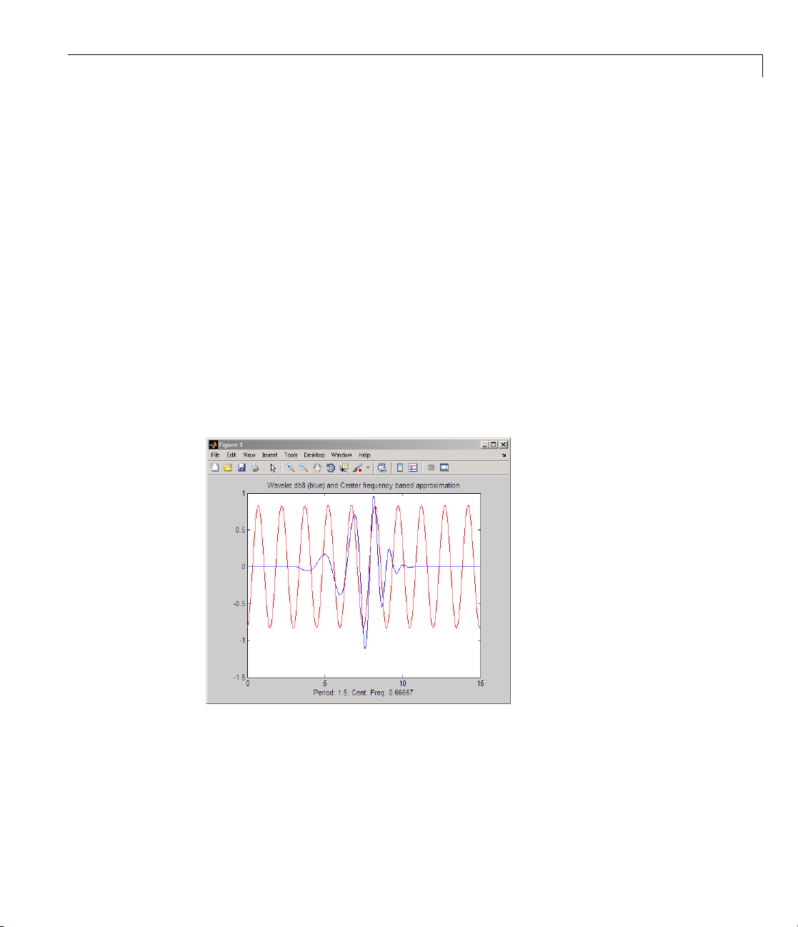
The basic approach identifies the pea k power in the Fourier transform of the
wavelet as its center frequency and divides that value by the product of the
scaleandthesamplinginterval. See
example shows the m atch between the estimated center frequency of the
scal2frq for details. The following
db8
wavelet and a sinusoid of the same frequency.
The relationship between scale and frequency in the CWT is also explored in
“CWT as a F iltering Technique” on page 1-27.
1-25
Page 36

1 Wavelets: A New Tool for Signal Analysis
Shifting
Shifting a wavelet simply means delaying (or advancing) its onset.
Mathematically, delaying a function f(t)byk is represented by f(t – k):
CWT as a Windowed Transform
In “Short-Time Fourier Transform” on page 1-16, the STFT is described as a
windowing of the signal to create a local frequency analysis. A shortcoming
oftheSTFTapproachisthatthewindowsizeisconstant. Thereisa
trade off in the choice of window size. A longer time window improves
frequency resolution while resulting in p oorer time resolution because the
Fourier transform loses all time resolution over the duration of the window.
Conversely, a shorte r time window improves time localization while resulting
in poorer frequency resolution.
1-26
Wavelet analysis represents the next logical step: a windowing technique with
variable-sized regions. Wavelet analysis allows the use of long time intervals
where you want more precise low-frequency information, and shorter regions
where you want high-frequency information.
following figure contrasts time, frequency, time-frequency, and time-scale
The
presentations of a signal.
re
Page 37

Continuous Wavelet Transform
CWT as a Filtering Technique
The continuous wavelet transform (CWT) computes the inner p roduct of a
signal,
().t
, with translated and dilated versions of an analyzing wav el et,
ft()
The definition of the CW T is:
Cabf t t ft
(,; (), ()) () ( )
∞
=
∫
−∞
1
*
tb
−
dt
a
a
You can also interpret the CWT as a frequency-based filtering of the signal by
rewriting the CWT as an inverse Fourier transform.
∞
Cabf t t a a e df
( , ; ( ), ( )) ( ) ( ))(
where
ˆ
and
()f
1
=
∫
−∞
2
ˆ
are the Fourier transforms of the signal and the
()
∧
∧
jb
*
wavelet.
From the preceding equations, you can s ee that stretching a wavelet in time
causes its support in the frequency domain to shrink. In addition to shrinking
the frequency support, the center frequency of the wavelet shifts toward lower
frequencies. The following figure demonstrates this effect for a hypothetical
wavelet and scale (dilation) factors of 1,2, and 4.
1-27
Page 38

1 Wavelets: A New Tool for Signal Analysis
ˆ
ψ(ω)
−ω
0
ω
0
√
2ˆψ(2ω)
−
ω
0
2
ω
0
2
√
4ˆψ(4ω)
ω
ω
0
0
−
This depicts the CWT as a bandpass filtering of the input signal. CWT
coefficients at lower scales represent energy in the input signal at higher
frequencies, w h ile CWT coefficients at higher scales represent energy in the
input signal at lower frequencies. However, unlike Fourier bandpass filtering,
the width of the bandpass filter in the CWT is inversely propo rtional to scale.
The width of the CWT filters decreases with increasing scale. This follows
from the uncertainty relationships between the time and frequency support of
a signal: the broader the support of a signal in time, the narrower its support
in frequency. The converse relationship also holds.
4
4
1-28
In the wavelet transform, the scale, or dilation operation is defined to
preserve energy. To preserve energy w hile shrinking the frequency support
requires that the peak energy level increases. The quality factor,orQfactor
of a filter is the ratio of its peak energy to bandwidth. Because shrinking
or stretching the frequency support of a wavelet results in commensurate
increases or decreases in its peak energy, wavelets are often referred to as
constant-Q filters.
Page 39

Continuous Wavelet Transform
Five Easy Steps to a Continuous Wavelet Transform
Here are the five steps of an easy recipe for creating a CWT:
1 Take a wavelet and compare it to a section at the start of the original signal.
2 Calculate a number, C, that represents how closely correlated the wavelet is
with this section of the signal. The larger the number
the more the similarity. This follows from the fact the CWT coefficients are
calculated with an inner product. See “Inner Products” on page 1-12 for
more information on how inner products measure similarity. If the signal
energy and the wavelet energy are equal to one,
a correlation coefficient. Note that, in general, the signal energy does
not equal one and the CWT coefficients are not directly interpretable as
correlation coefficients.
As described in “Definition of the Continuous Wavelet Transform” on page
1-20, the CWT coefficients explicitly depend on the analyzing wavelet.
Therefore, the CWT coefficients are different when you com pute the CWT
for the same signal using different wavelets.
C is in absolute value,
C may be interpreted as
3 Shiftthewavelettotherightandrepeat steps 1 and 2 until you’ve covered
the whole signal.
4 Scale (stretch) the wavelet and repeat steps 1 through 3.
1-29
Page 40

1 Wavelets: A New Tool for Signal Analysis
5 Repeat steps 1 through 4 for all scales.
Interpreting the CWT Coefficients
Because the CWT is a redundant transform and the CWT coefficients depend
on the wavelet, it can be challenging to interpret the results.
To help you in interpreting CW T coefficients, it is best to start with a simple
signal to analyze and an analyzing wavelet with a simple structure.
A signal feature that wavelets are very good at detecting is a discontinuity,
or singularity. Abrupt transitions in signals re sult in wavelet coeffi cients
with large absolute values.
1-30
For the signal create a shifted impulse. The impulse occurs at point 500.
x = zeros(1000,1);
x(500) = 1;
For the wavelet, pick the Haar wavelet.
[~,psi,xval] = wavefun('haar',10);
plot(xval,psi); axis([0 1 -1.5 1. 5]);
title('Haar Wavelet');
Page 41

Continuous Wavelet Transform
To compute the CWT using the Haar wavelet at scales 1 to 128, enter:
CWTcoeffs = cwt(x,1:128,'haar');
CWTcoeffs
CWT coefficients for one scale. There are 128 rows because the
to
cwt is 1:128. The column dimension of the matrix matches the length of
is a 128-by-1000 matrix. Each row of the matrix contains the
SCALES input
the input signal.
Recall that the CWT of a 1D signal is a function of the scale and position
parameters. To produce a plot of the CWT coefficients, plot position along the
x-axis, scale along the y-axis, and encode the magnitude, or size of the CWT
coefficients as color at each point in the x-y, or time-scale plane.
You can produce this plot using
cwt(x,1:128,'haar','plot');
colormap jet; colorbar;
cwt with the optional input argument 'plot'.
1-31
Page 42

1 Wavelets: A New Tool for Signal Analysis
The preceding figure was modified with text labels to explicitly show which
colors indicate large and small CWT coefficients.
You can also plot the size of the CWT coefficients in 3D with
cwt(x,1:64,'haar','3Dplot'); colormap jet;
1-32
where the number of scales has been reduced to aid in visualization.
Examining the CWT of the shifted impulse signal, you can see that the set of
large CWT coefficients is concentrated in a narrow region in the time-scale
plane at small scales centered around point 500. As the scale increases, the set
of large CWT coefficients becomes wider, but remains centered around point
500. If you trace the border of this region, it resembles the following figure.
Page 43

Continuous Wavelet Transform
This region is referred to as the cone of influence of the point t=500 for the
Haar w avelet. For a given point, the cone of influence shows you which CWT
coefficients are affected by the signal value at that point.
To understand the cone of influence, assume that you have a wavelet
supported on [-C, C]. Shifting the wavelet by b and scaling by a results in a
wavelet supported on [-Ca+b, Ca+b]. For the simple case of a shifted impulse,
, the CWT coefficients a re only nonzero in an interval around τ equal
()t −
to the support of the wavelet at each scale. You can see this by considering
the formal expression of the CWT of the shifted impulse.
Cab t t t
(,; ( ), ()) ( ) ( ) ( )
−=− =
∞
∫
−∞
11
**
tb
−−
dt
a
a
a
b
a
For the impulse, the CWT coefficients are equal to the conjugated,
time-reversed, and scaled wavelet as a function of the shift parameter, b.You
can see this by plotting the CWT coefficients for a select few scales.
subplot(311)
plot(CWTcoeffs(10,:)); title('Scale 10');
subplot(312)
plot(CWTcoeffs(50,:)); title('Scale 50');
subplot(313)
plot(CWTcoeffs(90,:)); title('Scale 90');
1-33
Page 44

1 Wavelets: A New Tool for Signal Analysis
The cone of influence depends on the wavelet. You can find and plot the cone
of influence for a specific wavelet with
The next example features the superposition of two shifted impulses,
()()tt−+−300 500
wavelet with four vanishing moments,
cone of influence for the points 300 and 500 using the
conofinf.
. In this case, use the Daubechies’ extremal phase
db4. The following figure shows the
db4 wavelet.
1-34
Look at point 400 for scale 20. At that scale, you can see that neither cone
of influence overlaps the point 400. Therefore, you can expect that the CWT
coefficientwillbezeroatthatpointand scale. The signal is only nonzero
at two values, 300 and 500, and neither cone of influence for those values
includes the point 400 at scale 20. You can confirm this by entering:
x = zeros(1000,1);
x([300 500]) = 1;
CWTcoeffs = cwt(x,1:128,'db4');
plot(CWTcoeffs(20,:)); grid on;
Page 45
Continuous Wavelet Transform
Next, look at the point 400 at scale 80. At scale 80, the cones of influence
for both points 300 and 500 include the point 400. Even though the signal
is zero at point 400, you obtain a nonzero CWT coefficient at that scale. The
CWT coefficient is nonzero because the support of the wavelet has become
sufficiently large at that scale to allow signal values 100 points above and
below to affect the CWT coefficient. You can confirm this by entering:
plot(CWTcoeffs(80,:));
grid on;
In the preceding example, the CWT coefficients became large in the vicinity
of an abrupt change in the signal. This ability to detect discontinuities is a
strength of the wavelet transfo rm. The preceding ex ample also demonstrated
1-35
Page 46

1 Wavelets: A New Tool for Signal Analysis
that the CWT coefficients localize the discontinuity best at small scales. At
small scales, the small support of the wavelet ensures that the singularity
only affects a small set of wavelet coefficients.
To demonstrate w hy the wavelet transform is so adept at detecting abrupt
changes in the signal, consider a shifted Heaviside, or unit step signal.
x = [zeros(500,1); ones(500,1)];
CWTcoeffs = cwt(x,1:64,'haar','plot'); colormap jet;
1-36
Similar to the shifted impulse example, the abrupt transition in the shifted
step function results in large CWT coefficients at the discontinuity. The
following f igure illustrates why this occurs.
Page 47
Continuous Wavelet Transform
A
B
C
In the preceding figure, the red function is the shifted unit step function. The
black functions labeled A, B, and C depict Haar wavelets at the same scale
but different positions. You can see that the CWT coefficients around position
A are zero. The s ignal is zero in that neighborhood and therefore the wavelet
transform i s also zero because any w av elet integrates to zero.
Note the Haar wavelet centered around position B. The negative part of the
Haar wavelet overlaps with a region of the step function that is equal to 1.
The CWT coefficients are negative because the product of the Haar w av elet
and the unit step is a negative constant. Integrating over that area yields a
negative number.
Note the Haar wavelet centered around position C. Here the CWT coefficients
are zero. The s tep function is equal to one. The product of the wavelet with
the step function is equal to the wavelet. Integrating any wavelet over its
support is zero. This is the zero moment property of wavelets.
At position B, the Haar wavelet has already shifted into the nonzero portion
of the step function by 1/2 of its support. As soon as the support of the wavelet
intersects with the unity portion of the step function, the CWT coefficients
are nonzero. In fact, the situation illustrated in the previous figure coincides
with the CWT coefficients achieving their largest absolute value. This i s
because the entire negative deflection of the wavelet oscillation overlaps with
the unity portion of the unit step while none of the positive deflection of the
wavelet does. Once the wavelet shifts to the point that the positive deflection
overlaps with the unit step, there will be some positive contribution to the
1-37
Page 48

1 Wavelets: A New Tool for Signal Analysis
integral. The wavelet coefficients are still negative (the negative portion of
the integral is larger in area), but they are smaller in absolute value than
those obtained at position B.
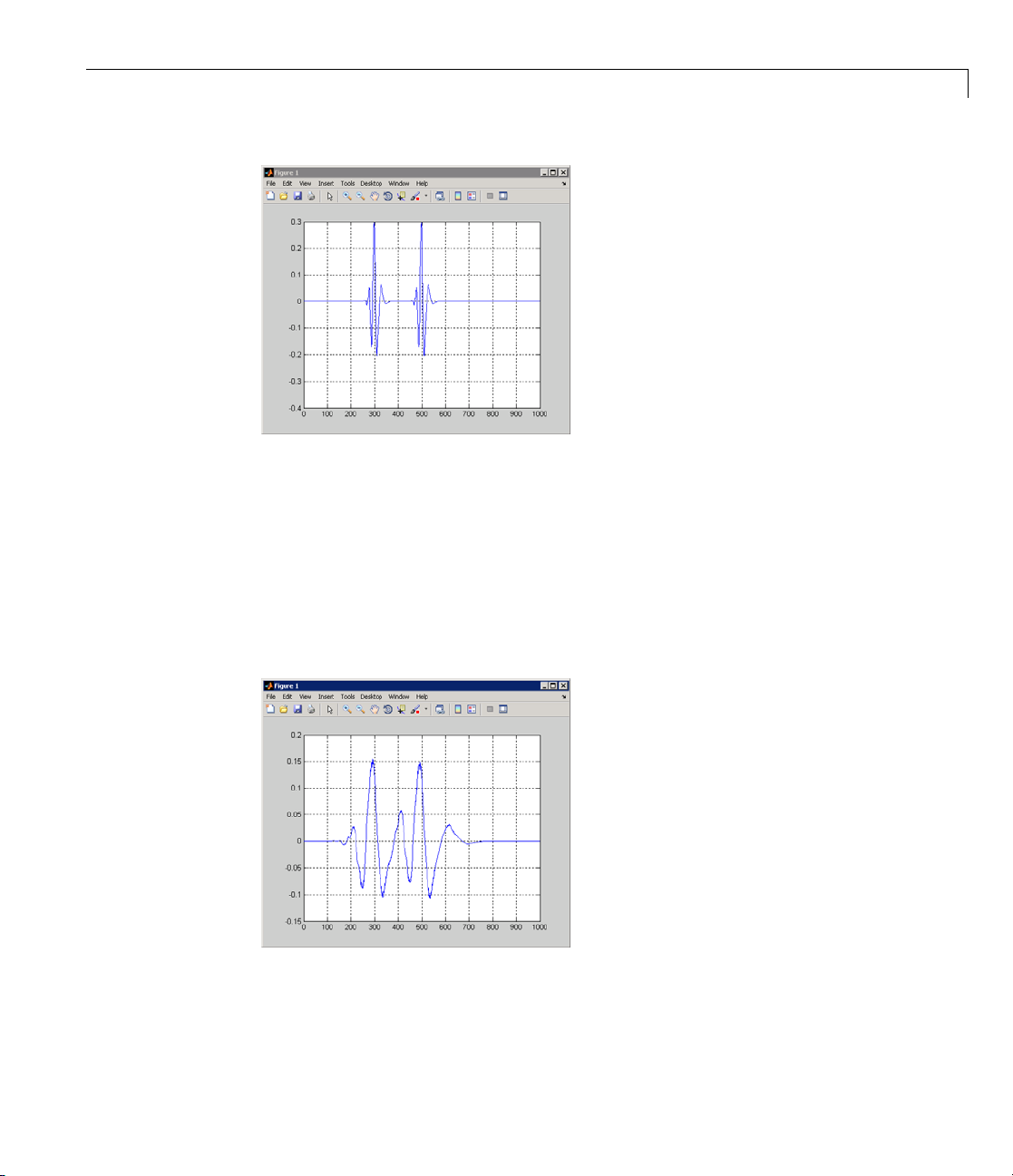
The following figure illustrates two other positions where the wavelet
intersects the unity portion of the unit step.
1-38
In the top figure, the wavelet has just begun to overlap with the unity portion
of the unit step. In this case, the CWT coefficien ts are negative, but not as
large in absolu t e value as those obtained at position B. In the bottom figure,
the wavelet has shifted past position B and the positive deflection of the
wavelet begins to contribute to the integral. The CWT coefficients are still
negative, but not as large in absolute value as those obtained at position B.
You can now visualize how the wavelet transform is able to detect
discontinuities. You can also visualize in this simple example exactly why the
CWT coefficients are negative in the CWT of the shifted unit step using the
Haar wavele t. Note that this behavior differs for other wavelets.
x = [zeros(500,1); ones(500,1)];
Page 49

Continuous Wavelet Transform
CWTcoeffs = cwt(x,1:64,'haar','plot'); colormap jet;
% plot a few scales for visualization
subplot(311);
plot(CWTcoeffs(5,:)); title('Scale 5');
subplot(312);
plot(CWTcoeffs(10,:)); title('Scale 10');
subplot(313);
plot(CWTcoeffs(50,:)); title('Scale 50');
Next consider how the CWT represents smooth signals. Because sinusoidal
oscillations are a common phenomenon, this section examines how sinusoidal
oscillations in the signal affect the CWT coefficients. To begin, consider the
sym4 wavelet at a spec ific scale superimposed on a sine wave.
Recall that the CWT coefficients are o btained by computing the product of
the signal with the shifted and scaled analyzing wavelet and integrating
the result. The following figure shows the product o f the wavelet and the
sinusoid from the preceding figure.
1-39
Page 50

1 Wavelets: A New Tool for Signal Analysis
You can see that integrating over this product produces a positive CWT
coefficient. That results because the oscillation in the w avelet approximately
matches a period of the sine wave. The wavelet is in phase with the sine wave.
The negative deflections of the wavelet approximately match the negative
deflections of the sine wave. The same is true of the positive deflections of
both the wavelet and sinusoid.
1-40
The following figure shifts the wavelet 1/2 of the period of the sine wave.
Examine the product of the shifted wavelet and the sinusoid.
Page 51

Continuous Wavelet Transform
You can see that integrating over this product produces a negative CWT
coefficient. That results because the wavelet is 1/2 cycle out of phase with the
sine wave. The negative deflections of the wavelet approximately match the
positive deflections of the sine wave. The positive deflections of the wavelet
approximately match the negative deflections of the sinusoid.
Finally, shift the wavelet approximately one quarter cycle of the sine wave.
The following figure shows the product of the shifted wavelet and the sinusoid.
1-41
Page 52

1 Wavelets: A New Tool for Signal Analysis
Integrating over this product produces a CWT coefficient much smaller in
absolute value than either of the two previous examples. That results because
the negative deflection of the wavelet approxima t el y ali gn s w ith a positi ve
deflection of the sine wave. Also, the main positive deflection of the wavelet
approximately aligns with a positive deflectio n of the sine wave. The resulting
product looks much more like a w avelet than the other two products. If it
looked exactly like a wavelet, the integral would be zero.
1-42
At scales where the oscillation in the wavelet occurs on either a much larger
or smaller scale than the period of the sine wave, you obtain CWT coefficients
near zero. The following figure illustrates the case where the wavelet
oscillates on a much smaller scale than the sinusoid.
Page 53

Continuous Wavelet Transform
The product shown in the bottom pane closely resembles the analyzing
wavelet. Integrating this product results in a CWT coefficient near zero.
The following example constructs a 60-Hz sine wave and obtains the CWT
using the
t = linspace(0,1,1000);
x = cos(2*pi*60*t);
CWTcoeffs = cwt(x,1:64,'sym8','plot'); colormap jet;
sym8 wavelet.
Note that the CWT coefficients are large in absolute value around scales 9
to 21. You can find the pseudo-frequencies corresponding to these scales
using the command:
freq = scal2frq(9:21,'sym8',1/1000);
Note that the CWT coefficients are large at scales near the frequency of the
sine wave. You can clearly see the sinusoidal pattern in the CWT coefficients
at these scales with the following code.
surf(CWTcoeffs); colormap jet;
shading('interp'); view(-60,12);
1-43
Page 54

1 Wavelets: A New Tool for Signal Analysis
Thefinalexampleconstructsasignalconsisting of both abrupt transitions
and s mooth oscillations. The signal is a 4-Hz sinusoid with two introduced
discontinuities.
N = 1024;
t = linspace(0,1,1024);
x = 4*sin(4*pi*t);
x = x - sign(t - .3) - sign(.72 - t);
plot(t,x); xlabel('t'); ylabel('x');
grid on;
1-44
Note the discontinuities near t=0.3 and t=0.7.
Page 55

Obtain and plot the CWT using the sym4 wavelet.
CWTcoeffs = cwt(x,1:180,'sym4');
imagesc(t,1:180,abs(CWTcoeffs));
colormap jet; axis xy;
xlabel('t'); ylabel('Scales');
Continuous Wavelet Transform
Note that the CWT detects both the abrupt transitions and oscillations in the
signal. The abrupt transitions affect the CWT coefficients at all scales and
clearly separate themselves from smoother signal features at small scales. On
the other hand, the maxima and minima of the 2–Hz sinusoid are evident in
the CWT coefficients at largescalesandnotapparentatsmallscales.
The following general principles are important to keep in mind when
interpreting CWT coefficients.
• Cone of influence— Depending on the scale, the CWT coefficient at a
point can be affected by signal values at points far removed. You have
to take into account the support of the wavelet at specific scales. Use
conofinf to determine the cone of influence. Not all wavelets are equal in
their support. For example, the Haar wavelet has smaller support at all
scales than the
sym4 wavelet.
• Detecting abrupt transitions— Wavelets are very useful for detecting
abrupt changes in a signal. Abrupt changes in a signal produce relatively
large wavelet coefficients (in absolute value) centered around the
discontinuity at all scales. Because of the support of the wavelet, the set
1-45
Page 56

1 Wavelets: A New Tool for Signal Analysis
of CWT coefficients affected by the singularity increases with increasing
scale. Recall this is the definition of the cone of influence. The most precise
localization of the discontinuity based on the CWT coefficients is obtained
at the smallest scales.
• Detecting smooth signal featu res— Sm ooth signal features produce
relatively large wavelet coefficients at scales where the oscillation in the
wavelet correlates best w ith the signal feature. For sinusoidal oscillations,
the CWT coefficients display an oscillatory pattern at scales where the
oscillationinthewaveletapproximates the period of the sine wave.
What’s Continuous About the Continuous Wavelet Transform?
Any signal processing performed on a computer using real-world data must be
performed on a discrete signal — that is, on a signal that has been measured
at discrete time. So what exactly is “continuous” about it?
What’s “continuous” about the CWT, and what distinguishes it from the
discrete wavelet transform (to be discussed in the following section), is the set
of scales and positions at which it operates.
1-46
Unlike the discrete wavelet transform, the CWT can operate at every scale,
from that of the original signal up to some maximum scale that you determine
by trading off your need for detailed analysis with available computational
horsepower.
The CWT is also continuous in terms of shifting: during computation, the
analyzing wavelet is shifted smoothly over the full domain of the analyzed
function.
Page 57

Discrete Wavelet Transform
Calculating wavelet coefficients at every possible scale is a fair amount of
work, and it generates an awful lot of data. What if we choose only a subset of
scales and positions at which to m ake our calculations?
It turns out, rather remarkably, that if we choose scales and positions based
on powers of two — so-called dyadic scales and positions — then our analysis
will be much more efficient and just as accurate. We obtain such an analysis
from the discrete wavelet transform (DWT). For more information on DWT,
see “Algorithms” in the Wavelet Toolbox User’s Guide.
An efficient way to implement this scheme using filters was developed in 1988
by Mallat (see [Mal89] in “References”). The Mallat algorithm is in fact a
classical scheme known in the signal processing community as a two-channel
subband coder (see page 1 of the book Wavelets and Filter Banks, by Strang
and Nguyen [StrN96]).
This very practical filtering algorithm yields a fast wavelet transform —a
box into which a signal passes, and out of which wavelet coefficients quickly
emerge. Let’s examine this in more depth.
Discrete Wavelet Transform
One-Stage Filtering: Approximations and Details
For many signals, the low-frequency content is the m ost important part. It is
what gives the signal its identity. The high-frequency content, on the other
hand, imparts flavor or nuance. Consider the human voice. If you remove
the high-frequency components, the voice sounds different, but you can still
tell what’s being said. However, if you remove enough of the low-frequency
components, you hear gibberish.
In wavelet analysis, w e often speak of approximations and details.The
approximations are the high-scale, low-frequency components of the signal.
The details are the low-scale, high-frequency components.
The filtering process, at its mos t basic level, looks like this.
1-47
Page 58

1 Wavelets: A New Tool for Signal Analysis
The original signal, S, passes through two co m plementary filters and emerges
as two signals.
Unfortunately, if we actually perform this operation on a real digital signal,
we wind up with twice as much data as we started with. Suppose, for instance,
that the original signal S consists of 1000 samples of data. Then the resulting
signals will each have 1000 samples, for a total of 2000.
These signals A and D are interesting, but we get 2000 values instead of the
1000wehad. Thereexistsamoresubtlewaytoperformthedecomposition
using wavelets. By looking carefully at the computation, we may keep
only one point out of two in each of the two 2000-length samples to get the
complete information. This is the notion of downsampling. We produce two
sequences called
cA and cD.
1-48
The process on the right, which includes downsampling, produces DWT
coefficients.
To gain a b etter appreciation of this process, let’s perform a one-stage discrete
wavelet transform of a signal. Our signal wil l be a pure sin u soid with
high-frequency noise added to it.
Page 59

Discrete Wavelet Transform
Here is our schematic diagram with real signals inserted into it.
The MATLA
s
= sin(20.*linspace(0,pi,1000)) + 0.5.*rand(1,1000);
[cA,cD] = dwt(s,'db2');
where db
Notice
requency noise, while the approximation coefficients
high-f
oise than does the original signal.
less n
[length(cA) length(cD)]
ans =
You m
fficient vectors are slightly more than half the length o f the original signal.
coe
s has to do with the filtering process, which is implemented by convolving
Thi
signal with a filter. The convolution “smears” the signal, introducing
the
eral extra samples into the result.
sev
B co de neede d to generate
2
isthenameofthewaveletwewanttousefortheanalysis.
that the detail coefficients
501 501
ay observe that the actual lengths of the detail and approximation
s, cD,andcA is
cD are small an d consist mainly of a
cA contain much
1-49
Page 60

1 Wavelets: A New Tool for Signal Analysis
Multiple-Level
The decompositi
being decompose
resolution com
Looking at a signal’s wavelet decomposition tree can yield valuable
information.
ponents. This is called the wavelet decomposition tree.
Decomposition
on proce ss can be iterated, with successive approximations
d in turn, so that one signal is broken down into m any lower
1-50
Number of Levels
nce the analysis process is iterative, in theory it can be continued
Si
definitely. In reality, the decomposition can proceed only until the
in
dividual details consist of a single sample or pixel. In practice, you’ll select
in
Page 61

Discrete Wavelet Transform
a suitable number of levels based on the nature of the signal, or on a suitable
criterion such as entropy (see “Choosing the Optimal Decomposition” in the
Wavelet Toolbox User’s Guide).
1-51
Page 62

1 Wavelets: A New Tool for Signal Analysis
Wavelet Reconstruction
We’ve learned how the discrete w avelet transform can be used to analyze,
or decompose, signals and images. This process is called d ecomposition
or analysis. The other half of the story is how those components can be
assembled back into the original signal without loss of information. This
processiscalledreconstruction,orsynthesis. The mathematical manipulation
that effe cts synthesis is called th e inverse discrete wavelet transform (IDWT).
To synthesize a signal using Wavelet Toolbox software, we reconstruct it
from the wavelet coefficients.
1-52
Where wavelet analysis involves filtering and downsampling, the wavelet
reconstruction process consists of upsampling and filtering. Upsampling is
the process of lengthening a signal component by i ns erting zeros between
samples.
The toolbox includes commands, like idwt an d waverec,thatperform
single-level or multilev el reconstruction, respectively, on the components of
one-dimensional signals. These commands have their two-dimensional and
three-dimensional analogs,
idwt2, wa verec2, idwt3,andwa vere c3.
Page 63

Wav elet R econstr uction
Reconstruction
The filtering pa
because it is the
reconstructio
The downsampl
decompositio
by carefully c
that are clos
aliasing.
A technical
of the book W
high-pass d
reconstru
mirror fil
rt of the reconstruction process also bears some discussion,
choice of filters that is crucial in achieving perfect
n of the original signa l.
ing of the signal components performed during the
n pha se introduces a distortion called aliasing. It turns out that
hoosing filters for the decomposition and reconstruction phases
ely related (but not identical), we can “cancel out” the effects of
discussion of how to design these filters is available on page 347
avelets and Filter Banks, by Strang and Nguyen. The low- and
ecomposition filters (
ction filters (
ters:
Filters
L and H), together with th eir associated
L' and H'), form a system of what is ca lled quadrature
Reconstructing Approximations and Details
We have seen that it is possible to reconstruct our original signal from the
coefficients of the approximations and details.
1-53
Page 64

1 Wavelets: A New Tool for Signal Analysis
It is also possible to reconstruct the a pproximations and details themselves
from their coefficient vectors. As an example, let’s consider how we would
reconstruct the first-level approximation
A1 from the coefficient vector cA1.
We pass the coefficient v ector
cA1 through th e same process we used to
reconstruct the original signal. However, i ns te ad of combining it with
the level-one detail
cD1, we feed in a vector of zeros in place of the detail
coefficients vector:
The process yields a reconstructed approximation A1, which has the same
length as the original signal
Similarly, we can reconstruct the first-level detail
S and which is a real approximation of it.
D1, using the analogous
process:
1-54
The reconstructed details and approximations are true constituents of the
original signal. In fact, we find when we combine them that
A
+ D1= S.
1
Note that the coefficient vectors
cA1 and cD1 — because they were produced
by downsampling and are only half the length of the original signal — cannot
Page 65

Wav elet R econstr uction
directly be combined to reproduce the signal. It is necessary to reconstruct the
approximations and details before combining them.
Extending this technique to the components of a multilevel analysis, we find
that similar relationships hold for all the reconstructed signal constituents.
That is, there are several ways to reassem ble the original signal:
Relationship of Filters to Wavelet Shapes
In the section “Reconstruction Filters” on page 1-53, we spoke of the
importance of choosing the right filters. In fact, the choice of filters not only
determines whether perfect reconstruction is possible, it also determines the
shape of the wavelet we use to perform the analysis.
To construct a wavelet of some practical utility, you seldom start by drawing a
waveform. Instead, it usually makes more sense to design the appropriate
quadrature m irror filters, and then usethemtocreatethewaveform. Let’s
see how this is done by focusing on an example.
Consider the low-pass reconstruction filter (
The filter coefficients can be o btained from the
L')forthedb2 wavelet.
dbaux function. By reversing
the order of the scaling filter vector and multiplying every even element
(indexing from 1) by (-1), you obtain the high-pass filter.
Repeatedly upsampling by two and convolving the output with the scaling
filter produces the Daubechies’ extremal phase wavelet.
L = dbaux(2);
H = wrev(L).*[1 -1 1 -1];
HU = dyadup(H,0);
1-55
Page 66
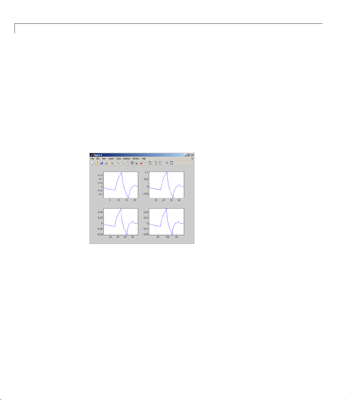
1 Wavelets: A New Tool for Signal Analysis
HU = conv(HU,L);
plot(HU); title('1st Iteration');
H1 = conv(dyadup(HU,0),L);
H2 = conv(dyadup(H1,0),L);
H3 = conv(dyadup(H2,0),L);
H4 = conv(dyadup(H3,0),L);
figure;
for k =1:4
subplot(2,2,k);
eval(['plot(H' num2str(k) ')']);
axis tight;
end
1-56
The curv e begins to lo ok progressively more like the db2 wavelet. This means
that the wavelet’s shape is determined entirely by the coefficients of the
reconstruction filters.
This relationship has profound implications. It means that you cannot choose
just any shape, call it a wavelet, and perform an analysis. At least, you can’t
choose an arbitrary wavelet waveform if you want to be able to reconstruct the
original signal accurately. You are compelled to choose a shape determined by
quadrature mirror decomposition filters.
Page 67
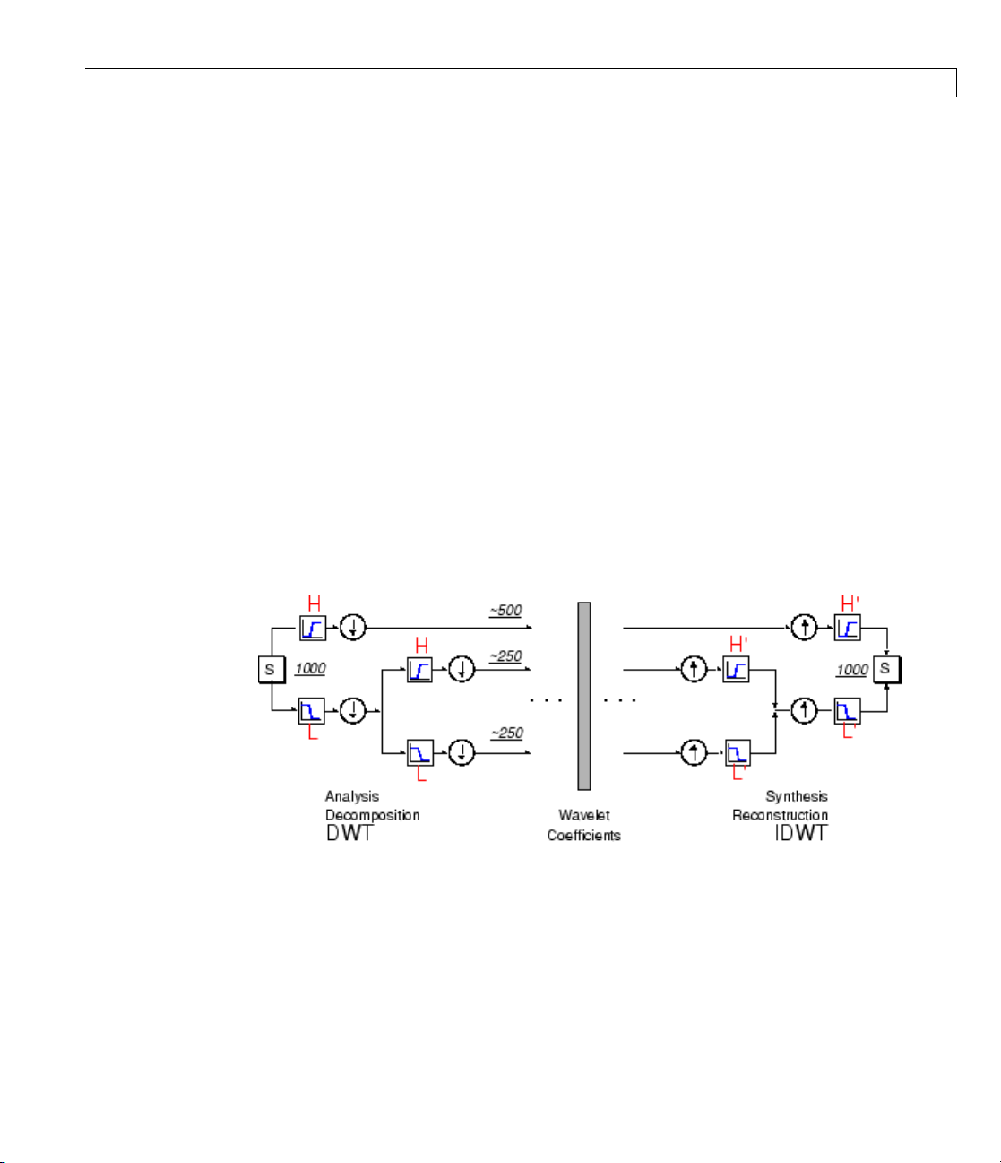
Wav elet R econstr uction
Scaling Function
We’ve seen the interrelation of wavelets and quadrature mirror filters. The
wavelet function ψ is determined by the high-pass filter, which also produces
the details of the wavelet decomposition.
There is an additional function associated with some, but not all, wavelets.
This is the so-called scaling function , ϕ. The scaling function is very similar
to the wavelet function. It is determined by the low-pass quadrature mirror
filters, and thus is associated with the approximations of the wavelet
decomposition.
In the same way that iteratively upsampling and convolving the
high-pass filter produces a shape approximating the wavelet function,
iteratively upsampling and convolving the low-pass filter produces a shape
approximating the scaling function.
Multistep Decomposition and Reconstruction
A m ultistep analysis-synthesis process can be represented a s
This process involves two aspects: breaking up a signal to obtain the wavelet
coefficients, and reassembling the signal from the coefficients.
We’ve already discussed decomposition and reconstruction at some length. Of
course, there is no point breaking up a signal merely to have the satisfaction
of immediately reconstructing it. We may modify the wavelet coefficients
before performing the reconstruction step. We perform wavelet analysis
1-57
Page 68

1 Wavelets: A New Tool for Signal Analysis
because the coefficients thus obtained have many known uses, de-noising and
compression being foremost among them.
But wavelet analysis is still a new and emerging field. No doubt, many
uncharted uses of the wavelet coefficients lie in wait. The toolbox can be
a means of exploring possible uses and hitherto unknown applications of
wavelet analysis. Explore the toolbox functions and see what you discover.
1-58
Page 69

WaveletPacketAnalysis
The wavelet packet method is a generalization of w avelet decomposition that
offers a richer range of possibilities for signal analysis.
In wavelet analysis, a signal is split into an approximation and a detail.
The approximation is then itself split i nto a second-level approximation and
detail, and the process is repeated. F or an
n+1 possible ways to decompose or encode the signal.
Wavelet Packet Ana lysis
n-level decomposition, there are
In wavel
be split
This yields more than
et packet analysis, the details as well as the approximations can
.
1n −
2
2
differentwaystoencodethesignal. Thisisthe
wavelet packet decomposition tree.
The w avelet decomposition tree is a part of this comple te binary tree.
1-59
Page 70

1 Wavelets: A New Tool for Signal Analysis
Forinstance,waveletpacketanalysisallowsthesignalStoberepresentedas
A1 + AAD3 + DAD3 + DD2. This is an example of a representation that is not
possible with ordinary wavelet analysis.
Choosing one out of all these possible encodings presents an interesting
problem. In this toolbox, we use an entropy-based criterion to select the
most suitable de composition of a given signal. This means we look at each
node of the decomposition tree and quantify the information to be gained by
performing each split.
1-60
Simple and efficient algorithms exis t for both wavelet packet decomposition
and optimal decomposition selection. This toolbox uses an adaptive filtering
algorithm, based on work by Coifman and Wickerhauser (see [CoiW92] in
“References”), with direct applications in optimal signal coding and data
compression.
Such algorithms allow the Wavelet Packet 1-D and Wavelet Packet 2-D
tools to include “Best L ev el” and “Best Tree” features that optimize the
decomposition both globally and with respect to each node.
Page 71

History of Wavelets
From an historical point of view, wavelet analysis is a new method, though
its mathematical underpinnings date back to the work of Joseph Fourier in
the nineteenth century. Fourier laid the foundations with his theories of
frequency analysis, which proved to be enormously important and influential.
The attention of researchers gradually tu rned from frequency-based analysis
to scale-based analysis when it started to become clear that an approach
measuring average fluctuations at different scales might prove less sensitive
to noise.
The first recorded mention of w hat we now call a “wavelet” seems to be in
1909, in a thesis by Alfred Haar.
The concept of wavelets in its presen t theoretical f orm was first proposed
by Jean Morlet and the team at the Marseille Theoretical Physics Center
working under Alex Grossmann in France.
History of Wavelets
The methods of wavelet analysis have been developed mainly by Y. Meyer
and his colleagues, who have ensured the methods’ disseminatio n. The main
algorithm dates back to the work of Stephane Mallat in 1988. Since then,
research on wavelets has become international. Such research is particularly
active in the United States, where it is spearheaded by the work of scientists
such as Ingrid Daubechies, Ronald Coifman, and V ictor Wickerhauser.
Barbara B urke Hubbard describes the birth, the history, and the seminal
concepts in a very clear text. See The World A ccording to Wavelets, A.K.
Peters, Wellesley, 1996.
The w avelet domain is g r owing up very quickly . A lot of mathematical papers
and practical trials are published every month.
1-61
Page 72

1 Wavelets: A New Tool for Signal Analysis
Introduction to the Wavelet Families
Several families of wavelets that haveproventobeespeciallyusefulare
included in this toolbox. What follows is an introduction to some wavelet
families.
• “Haar” on page 1-63
• “Daubechies” on page 1-64
• “Biorthogonal” on page 1-65
• “Coiflets” on pag e 1-67
• “Symlets” on page 1-67
• “Morlet” on page 1-68
• “Mexican Hat” on page 1-68
• “Meyer” on page 1-69
• “Other Real Wavelets” on page 1-69
1-62
• “Complex Wavelets” on page 1 -69
To ex plore all wavelet families on your own, check out the Wavelet Display
tool:
1 Type wavemenu at the MATLAB command line. The Wavelet Toolbox
Main Menu appears.
Page 73

Introduction to the Wavelet Families
2 Click the Wavelet Display menu item. The Wavelet Display tool
appears.
3 Select a family from the Wavelet menu at the top right of the tool.
4 Click the Display button. Pictures of the w avelets and their associated
filters appear.
5 Obtain more information by clicking the information buttons located at
the right.
Haar
Any discussion of wav el ets begins with Haar wavelet, the first and sim plest.
Haar wavelet is discontinuous, and resembles a step function. It represents
1-63
Page 74

1 Wavelets: A New Tool for Signal Analysis
the same wavelet as Daubechies db1. See “Haar” in the Wavelet Toolbox
User’s Guide for more detail.
Daubechies
Ingrid Daub
invented w
making dis
echies, one of the brightest stars in the world of wavelet research,
hat are called compactly supported orthonormal wavelets — thus
crete wavelet analysis practicable.
The names
order, an
above, is
the next
You can obtain a survey of the main properties of this family by ty ping
waveinfo('db') from the MATLAB command line. See “Daubechies
Wavelets: dbN” in the Wavelet Toolbox User’s Guide for more detail.
of the Daubechies family wavelets are written
d
db the “surname” of the wavelet. The db1 wavelet, as mentioned
the same as
nine members of the family:
Haar wavelet. Here are the wavelet functions psi of
dbN,whereN is the
1-64
Page 75

Biorthogonal
This family of wa
needed for signa
decomposition
side) instead o
l and image reconstruction. By using two wavelets, one for
(on th e left side) and the other for reconstruction (on th e right
f the same single one, interesting properties are derived.
Introduction to the Wavelet Families
velets exhibits the property of linear phase, which is
1-65
Page 76
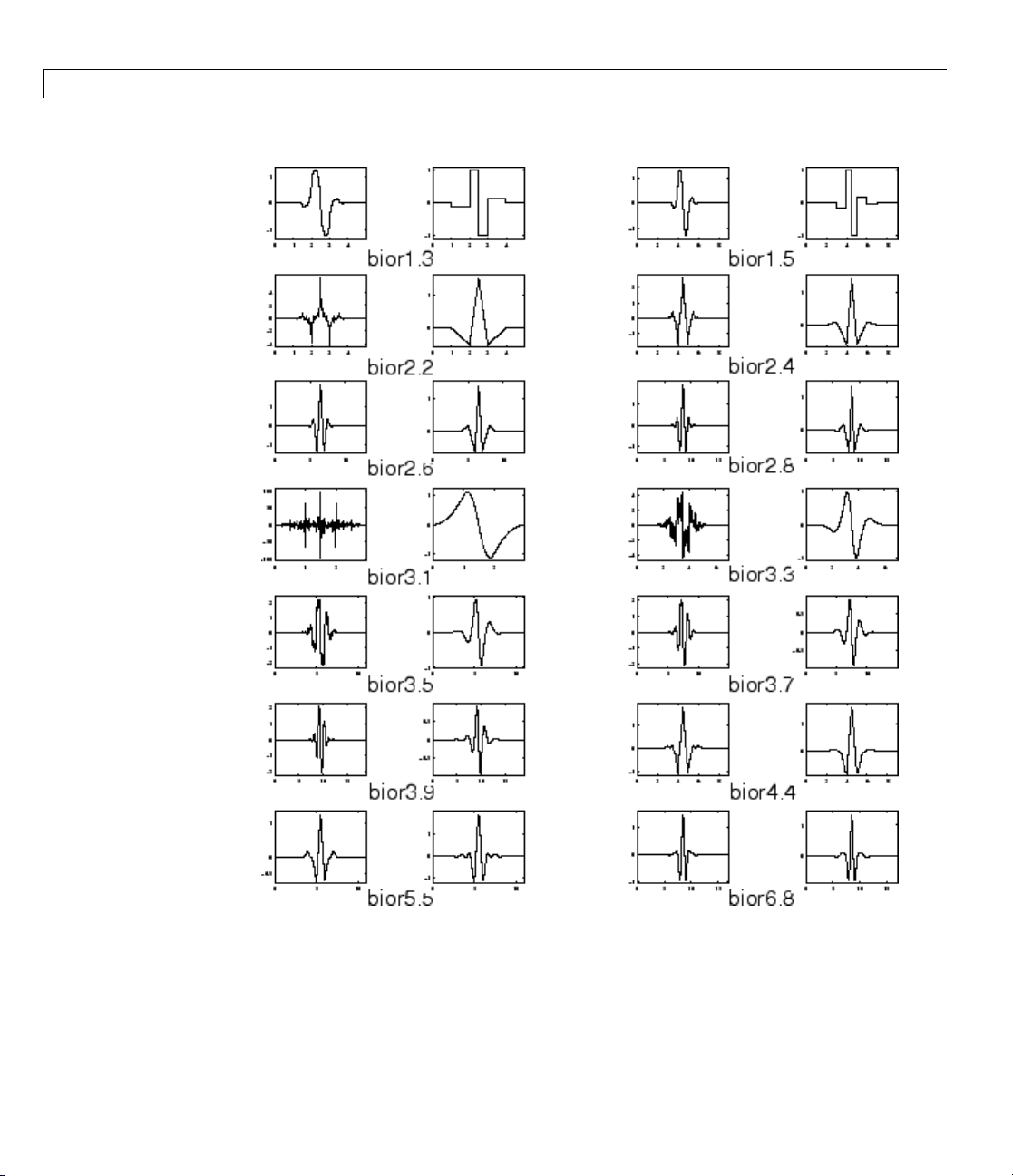
1 Wavelets: A New Tool for Signal Analysis
1-66
You can obtain a survey of the main properties of this family by ty ping
waveinfo('bior') from the MATLAB command line. See “Biorthogonal
Wavelet Pairs: biorNr.Nd” in the Wavelet Toolbox User’s Guide for more detail.
Page 77

Introduction to the Wavelet Families
Coiflets
Built by I. Daubechies at the request of R. Coifman. The wavelet function has
2N moments equal to 0 and the scaling function has 2N-1 moments equal to
0. Thetwofunctionshaveasupportoflength6N-1. You can obtain a survey
of the main properties of this family by typing
MATLAB command line. See “Coiflet Wavelets: coifN” in the Wavelet Toolbox
User’s Guide for more detail.
waveinfo('coif') from the
Symlets
The symlets are nearly symmetrical wavelets proposed by Daubechies as
modifications to the
similar. Here are the wavelet functions psi.
db family. The properties of the two wavelet families are
You can obtain a survey of the main properties of this family by ty ping
waveinfo('sym') from the MATLAB command line. See “Symlet Wavelets:
symN” in the Wavelet Toolbox User’s Guide for more detail.
1-67
Page 78

1 Wavelets: A New Tool for Signal Analysis
Morlet
This wavelet has
You can obtain a survey of the main properties of this family by ty ping
waveinfo('morl') from the MATLAB command line. See “Morlet Wavelet:
morl” in the Wavelet Toolbox User’s G uide for more detail.
no scaling function, but is explicit.
1-68
Mexican Hat
This wavelet has no scaling function and is derived from a function that is
proportional to the s econd deriv ative function of the Gaussian probability
density function.
You can obtain a survey of the main properties of this family by ty ping
waveinfo('mexh') from the MATL AB command line. See “Mex ican Hat
Wavelet: mexh” in the Wavelet Toolbox User’s Guide for more information.
Page 79

Introduction to the Wavelet Families
Meyer
The Meyer wavelet and scaling function are defined in the frequency domain.
You can obtain a survey of the main properties of this family by ty ping
waveinfo('meyer') from the MATLA B command line. See “Meyer Wavelet:
meyr” in the Wavelet Toolbox User’s Guide for more detail.
Other Real Wavelets
Some other r eal wavelets are available in the toolbox:
• Reverse B iorthogonal
• Gaussian derivatives family
• FIR based approximation of the Meyer wavelet
See “Additional Real Wavelets” in the Wavelet Toolbox User’s Guide for more
information.
Complex Wavelets
Some com plex wavelet families are available in the toolbox:
• Gaussian derivatives
• Morlet
• Frequency B-Spline
1-69
Page 80

1 Wavelets: A New Tool for Signal Analysis
• Shannon
See “Complex W av elets” in the Wavelet Toolbox User’s Guide for more
information.
1-70
Page 81

Using Wavelets
This chapter takes you step-by-step through examples that teach you how to
use the graphical tools and command-line functions.
• “Introduction to Wavelet T oolbo x GUIs and Functions” on page 2-3
• “One-Dimensional Continuous Wavelet Analysis” on page 2-4
• “One-Dimensional Complex Continuous Wavelet Analysis” on page 2-19
• “One-Dimensional Discrete Wavelet Analysis” on page 2-28
• “Two-Dimensional Discrete Wavelet Analysis” on page 2-63
2
• “Wavelets: Working with Images” on page 2-90
• “One-Dimensional Discrete Stationary Wavelet Analysis” on page 2-97
• “Two-Dimens iona l Discrete Stationary Wavelet Analysis” on page 2-113
• “One-Dimensional Wavelet Regression Estimation” on page 2-130
• “One-Dimensional Wavelet Density Estimation” on page 2-140
• “One-Dimensional Variance Adaptive Thresholding of Wavelet Coefficients”
on page 2-148
• “One-Dimensional Selection of Wavelet Coefficients Using the Graphical
Interface” on page 2-158
• “Two-Dim ensional Selection of Wavelet Coefficients Using the Graphical
Interface” on page 2-167
• “One-Dimensional Extension” on page 2-175
• “Two-Dimensional Extension” on page 2-183
• “Image Fusion” on page 2-187
• “One-Dimensional Fractional Bro wnian Motion Synthesis” on page 2-196
Page 82

2 Using Wavelets
• “New Wavelet for CWT” on page 2-204
• “Multivariate Wavelet De-Noising” on page 2-216
• “Multiscale Principal Components Analysis” o n page 2-233
• “One-Dimensional Multisignal Analysis” on page 2-247
• “Two-Dimensional True Compression” on page 2-301
• “Three-Dimensional Discrete Wavelet Analysis” on page 2-322
2-2
Page 83

Introduction to Wavelet Toolbox™ GUIs and Functions
Introduction to Wavelet Toolbox GUIs and Functions
Wavelet Toolbox software contains graphical tools and command-line
functions that let you
• Examine and explore properties of individual w avelets and wavelet packets
• Examine statistics of signals and signal components
• Perform a continuous wavelet transform of a one-dimensional signal
• Perform discrete analysis and synthesis of one- and tw o-dimensional
signals
• Perform wavelet packet analysis of one- and two-dimensional signals (see
“Using Wavelet Packets” in the Wavelet Toolbox User’s Guide)
• Compress and remove noise from signals and images
In addition to the above, the toolbox makes it easy to customize the
presentation and visualization of your data. You choose
• Which signals to display
• A region of interest to magnify
• A coloring scheme for display of wavelet coefficient details
Note All the graphical user interface tools described in this chapter let
you import information from and export information to either disk or
workspace. For more information, see “File Menu Options” in the Wavelet
Toolbox User’s Guide.
2-3
Page 84

2 Using Wavelets
One-Dimensional Continuous Wavelet Analysis
This section takes you through the features of continuous wavelet analysis
using Wavelet Toolbox software.
The too lbox requires only one function for continuous wavelet analysis:
You’ll find full info rmation about this function in its refere nce page.
In this section, you’ll learn how to
• Load a signal
• Perform a continuous wavelet transform of a signal
• Produce a plot of the coefficients
• Produce a plot of coefficients at a given scale
• Produce a plot of local maxima of coefficients across scales
• Select the displayed plots
• Switch from scale to pseudo-frequency information
• Zoom in on detail
• Display coefficients in normal or absolute mode
• Choose the scales at which analysis is performed
Since you can perform analyses either from the command line or using the
graphical interface tools, this section has subsections covering each method.
The final subsection discusses how to exchange signal and coefficient
information between the disk and the graphical tools.
cwt.
2-4
Page 85
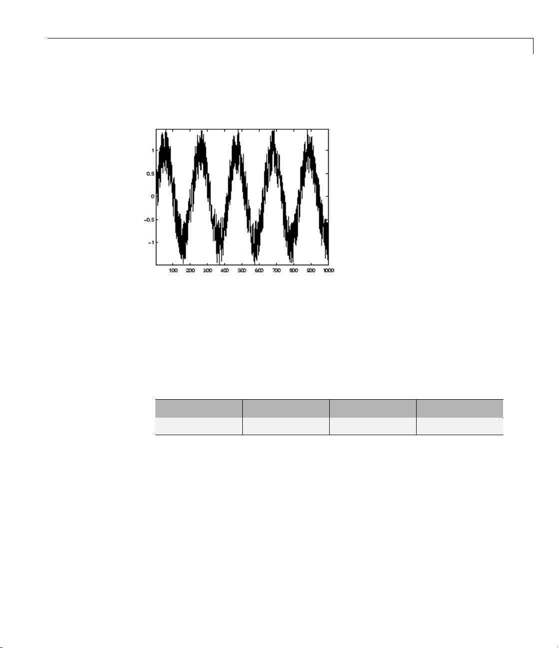
One-Dimensional Continuous Wavelet Analysis
Continuous Anal
This example inv
1 Load a signal.
olves a noisy sinusoidal signal.
ysis Using the Command Line
From the MATLAB prompt, type
load noissin;
You now have the signal noissin in your workspace:
whos
Name
noissin 1x1000 8000 double array
2 Perform a Continuous Wavelet Transform.
Use the
cwt command. Type
c = cwt(noissin,1:48,'db4');
Size
Bytes
Class
The arguments to cw t specify the signal to be analyzed, the scales of the
analysis, and the wavelet to be used. The returned argument
the coefficients at various scales. In this case,
c is a 48-by-1000 matrix with
c contains
each row corresponding to a s ingle scale.
2-5
Page 86

2 Using Wavelets
3 Plot the coefficients.
The
cwt comm and accepts a fourth argument. This is a flag that, when
present, causes
cwt to produce a plot o f the absolute values of the
continuous wavelet transform coefficients.
The
cwt command can accept more arguments to define the different
characteristics of the produced plot. For more information, see the
reference page.
c = cwt(noissin,1:48,'db4','plot');
Aplotappears.
cwt
2-6
Of course, coe fficient plots generated from the command line can be
manipulated using ordinary MATLAB graphics commands.
4 Choose scales for the a nalys is.
The second argument to
cwt gives you fine control over the scale levels on
which the continuous analysis is performed. In the previous example, w e
used all scales from 1 to 48, but you can construct any scale vector subject
to these constraints:
Page 87
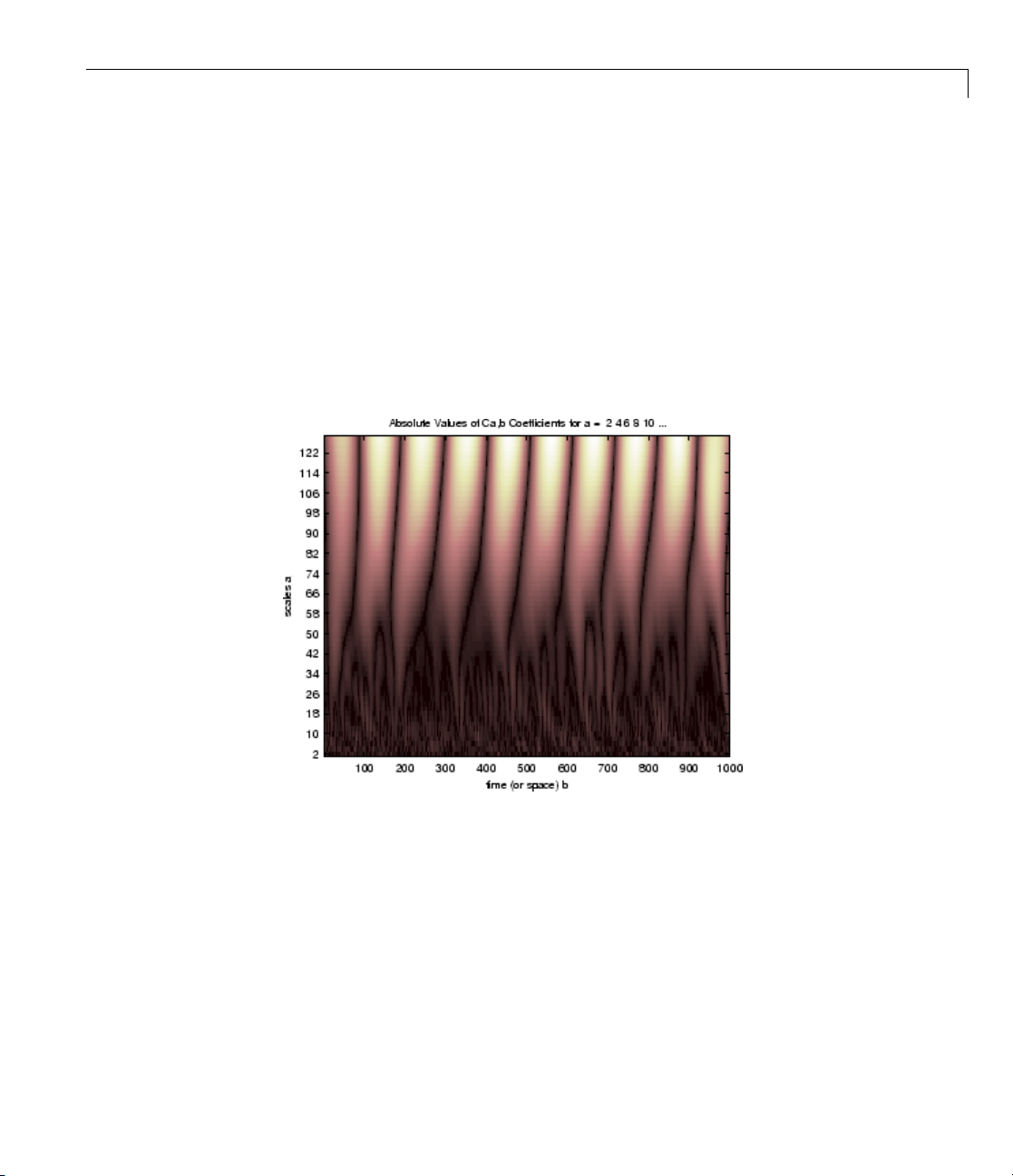
One-Dimensional Continuous Wavelet Analysis
• All scales must be real positive numbers.
• The scale increment must be positive.
• The highest scale cannot exceed a maximum value depending on the
signal.
Let’s repeat the analysis using every other scale from 2 to 128. Type
c = cwt(noissin,2:2:128,'db4','plot');
A new plot appears:
This plot gives a clearer picture of what’s happening with the signal,
highlighting the periodicity.
Continuous Analysis Using the Graphical Interface
We now use the Continuous W avelet 1-D tool to analyze the same noisy
sinusoidal signal we examined earlier using the command line interface in
“Continuous Analysis Using the Command Line” on pag e 2-5.
1 Start the Continuous Wavelet 1-D Tool. From the MATLAB prompt, type
2-7
Page 88

2 Using Wavelets
wavemenu
The Wavelet Toolbox Main Menu appears.
2-8
Click the Continuous Wavelet 1-D menu item.
The continuous wavelet analysis tool for one-dimensional signal data
appears.
Page 89

One-Dimensional Continuous Wavelet Analysis
2 Load a signal.
Choose the File > Load Signal menu option.
When the Load Signal dialog box appears, select the demo
MAT-file
toolbox/wavelet/wavedemo.ClicktheOK button.
noissin.mat, which should reside in the MATLAB folder
The noisy sinusoidal signal is loaded into the Continuous Wavelet 1-D
tool.
Thedefaultvalueforthesamplingperiodisequalto1(second).
3 Perform a Continuous Wavelet Transform.
2-9
Page 90

2 Using Wavelets
To start our analysis, let’s perform an analysis using the db4 wavelet at
scales 1 through 48, just as we did using command line functions in the
previous section.
In the upper right portion of the Continuous Wavelet 1-D tool, select the
db4 wavelet and scales 1–48.
2-10
4 Click the Analyze button.
After a pause for computation, the tool displays the coefficients plot, the
coefficients line plot corresponding to the scale a = 24, and the local maxima
plot, which displays the chaining across scales (from a = 48 down to a = 1)
of the coefficients local maxima.
Page 91

One-Dimensional Continuous Wavelet Analysis
5 View Wavelet Coefficients Line.
Select a
right mo
desire
nother scale a = 40 by clicking in the coefficients plot with the
use button. See step 9 to know, more precisely, how to select the
dscale.
Click the New Coefficients Line button. The tool updates the plot.
6 View Maxima Line.
Click the Refresh Maxima Line button. The local maxima plot displays
the chaining across scales of the coefficients local maxima from a = 40
down to a = 1.
2-11
Page 92
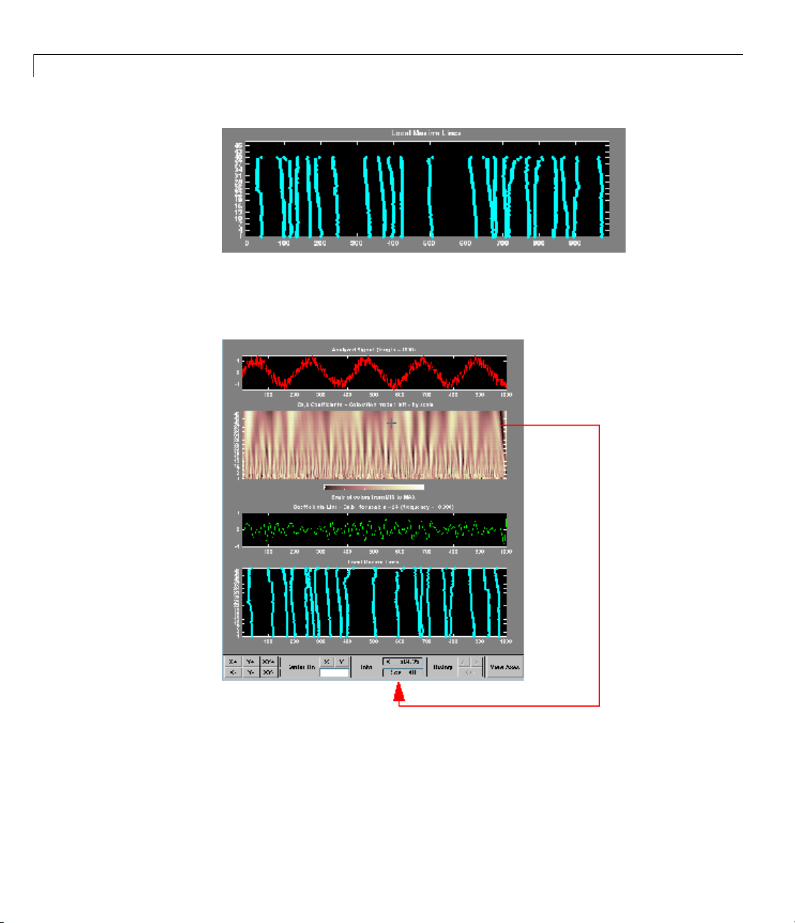
2 Using Wavelets
Hold down the right mouse button over the coefficients plot. The position of
the mouse is given by the Info frame (located at the bottom of the screen)
in terms of location (X)andscale(Sca).
2-12
7 Switch from scale to Pseudo-Frequency Information.
Using the option button on the right part of the screen, select Frequencies
instead of Scales. Again hold down the right mouse button over the
Page 93

One-Dimensional Continuous Wavelet Analysis
coefficients plot, the position of the mouse is g iven in terms of locatio n
(X) and frequency (Frq)inHertz.
This facility allows you to interpret scale in terms of an associated
pseudo-frequency, which depends on the wavelet and the sampling period.
For more information on the connection between scale and frequency, see
“How to Connect Scale to Frequency?” in the Wavelet Toolbox User’s Guide.
8 Deselect the last two plots using the check boxes in the Selected Axes
frame.
2-13
Page 94

2 Using Wavelets
9 Zoom in on detail.
2-14
Drag a rubber band box (by holding down the left mouse button) over the
portion of the signal you want to magnify.
10 Click the X+ button (located at the bottom of the screen) to zoom
horizontally only.
Page 95

One-Dimensional Continuous Wavelet Analysis
The Continuous Wavelet 1-D tool enlarges the displayed signal and
coefficients plot (for more informationonzooming,see“ConnectionofPlots”
in the Wavelet Toolbox User’s Guide).
As with the command line analysis on the preceding pages, you can change
the scales or the analyzing wavelet and repeat the analysis. To do this, just
edit the necessary fields and click the Analyze button.
11 View normal or absolute coefficients.
The Continuous Wavelet 1-D tool allows you to plot either the absolute
values o f the wavelet coefficients, or the coefficients themselves.
More generally, the coefficients coloration can be d one in several different
ways. For more details on the Coloration Mode, see “Controlling the
Coloration Mode”.
Choose either one of the absolute modes or normal modes from the
Coloration Mode menu. In n ormal modes, the colors are scaled between
the minimum and maximum of the coefficients. In absolute modes, the
2-15
Page 96

2 Using Wavelets
colors are scaled between zero and the maximum absolute value of the
coefficients.
The coefficients plot is redisplayed in the mode you select.
Importing and Exporting Information from the Graphical Interface
The Continuous Wavelet 1-D graphical interface tool lets you import
information from a nd export information to disk.
2-16
You can
• Load signals from disk into the Continuous Wavelet 1-D tool.
• Save wavelet coefficients from the Continuous Wavelet 1-D tool to disk.
Loading Signals into the Continuous Wavelet 1-D Tool
To load a signal you’ve constructed in your MATLAB workspace into the
Continuous Wavelet 1-D tool, save the signal in a MAT-file (with extension
mat or other).
For instance, suppose you’ve designed a signal called
analyze it in the Continuous Wavelet 1-D tool.
save warma warma
The workspace variable warma must be a vector.
sizwarma = size(warma)
warma and want to
Page 97

One-Dimensional Continuous Wavelet Analysis
sizwarma =
1 1000
To load this signal into the Continuous Wavelet 1-D tool, use the menu
option File > Load Signal. A dialog box appears that lets you select the
appropriateMAT-filetobeloaded.
Note The first one-dimensional variable encountered in the file is considered
the signal. Variables are inspected in alphabetical order.
Saving Wavelet Coefficients
The Continuous Wavelet 1-D tool lets you save wavelet coefficients to disk.
The toolbox creates a MAT-file in the current folder with the extension
and a name you give it.
To save the continuous wavelet coefficients from the present analysis, use the
menu option File > Save > Coefficients.
wc1
A dialog box appears that lets you specify a folder and filename for storing
the coefficients.
Consider the example analysis:
File > Example Analysis > with haar at scales [1:1:64] → Cantor curve.
After saving the continuous wavelet coefficients to the file
cantor.wc1,load
the variables into your workspace:
load cantor.wc1 -mat
whos
Name Size Bytes Class
coeff 64x2188 1120256 double array
scales 1x64 512 double array
wname 1x4 8 char array
2-17
Page 98

2 Using Wavelets
Variables coefs and scales contain the continuous wavelet coefficients
and the associated scales. M ore precisely, in the above example,
64-by-2188 matrix, one row for each scale; and
1:64. Variable wname contains the w avelet name.
scales is the 1-by-64 vector
coefs is a
2-18
Page 99

One-Dimensional Complex Continuous Wavelet Analysis
One-Dimensional Complex Continuous Wavelet Analysis
This section takes you through the features of complex continuous wavelet
analysis using the Wavelet Toolbox software and focuses on the differences
between the real and complex continuous analysis.
You can refer to the section “One-Dimensional Continuous Wavelet Analysis”
on page 2-4 if you want to learn how to
• Zoom in on detail
• Display coefficients in normal or absolute mode
• Choose the scales at which the analysis is performed
• Switch from scale to pseudo-frequency information
• Exchange signal and coefficient information between the disk and the
graphical tools
Wavelet T oolbox software requires only one function for complex continuous
wavelet analysis of a real valued signal:
about this function in its reference page.
cwt. You’llfindfullinformation
In this section, you’ll learn how to
• Load a signal
• Perform a complex continuous wavelet transform of a signal
• Produce plots of the coefficients
Since you can perform analyses either from the command line or using the
graphical interface tools, this section has subsections covering each method.
2-19
Page 100
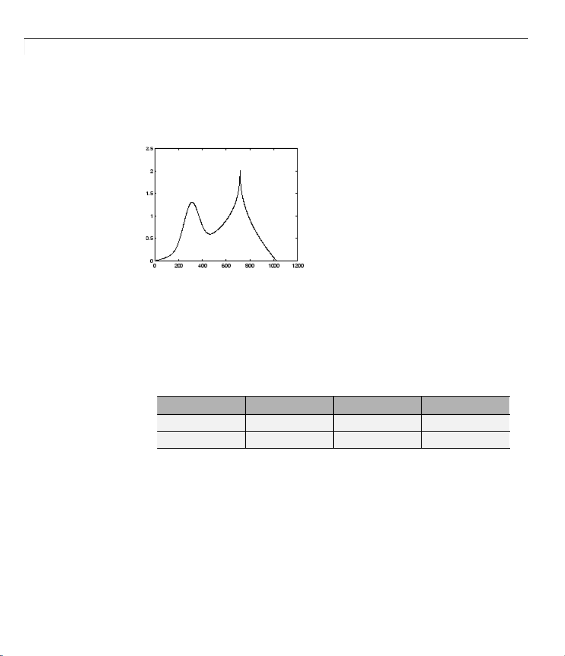
2 Using Wavelets
Complex Continu
ous Analysis Using the Command
Line
This example inv
1 Load a signal.
From the MATLAB prompt, type
load cus
You n ow have the signal cuspamax in your workspace:
whos
olves a cusp signal.
pamax;
2-20
Name Size Bytes Class
on
capti
amax
cusp
tion
cap
tion =
cap
x=l
y=
caption
erform a Continuous Wavelet Transform.
2 P
is a string that contains the signal definition.
1x71 142 char a
24
1x10
inspace(0,1,1024);
exp(-128*((x-0.3).^2))-3*(abs(x-0.7).^0.4);
8192 doub
rray
le array
 Loading...