Mathworks SYSTEM IDENTIFICATION TOOLBOX 7 Installation Guide

Download

System Identification Toolbox™ 7

Getting Started Guide

Lennart Ljung

How to Contact The MathWorks

www.mathworks. comp.soft-sys.matlab Newsgroup www.mathworks.com/contact_TS.html Technical Support

suggest@mathworks.com Product enhancement suggestions

bugs@mathwo doc@mathworks.com Documentation error reports service@mathworks.com Order status, license renewals, passcodes

info@mathwo

com

rks.com

Web

Bug reports

Sales, prici

ng, and general information

508-647-7000 (Phone)

508-647-7001 (Fax)

The MathWorks, Inc. 3 Apple Hill Drive Natick, MA 01760-2098

For contact information about worldwide offices, see the MathWorks Web site.

System Identification Toolbox™ Getting Started Guide

The software described in this document is furnished under a license agreement. The software may be used or copied only under the terms of the license agreement. No part of this manual may be photocopied or reproduced in any form without prior written consent from The MathW orks, Inc.

FEDERAL ACQUISITION: This provision applies to all acquisitions of the Program and Documentation by, for, or through the federal government of the United States. By accepting delivery of the Program or Documentation, the government hereby agrees that this software or d ocumentation qualifies as commercial computer software or commercial computer software documentation as such terms are used or defined in FAR 12.212, DFARS Part 227.72, and DFARS 252.227-7014. Accordingly, the terms and conditions of this Agreement and only those rights specified in this Agreement, shall pertain to and govern theuse,modification,reproduction,release,performance,display,anddisclosureoftheProgramand Documentation by the federal government (or other entity acquiring for or through the federal government) and shall supersede any conflicting contractual terms or conditions. If this License fails to meet the government’s needs or is inconsistent in any respect with federal procurement law, the government agrees to return the Program and Docu mentation, unused, to The MathW orks, Inc.

Trademarks

MATLAB and Simulink are registered trademarks of The MathWorks, Inc. See

www.mathworks.com/trademarks for a list of additional trademarks. Other product or brand

names may be trademarks or registered trademarks of their respective holders.

Patents

The MathWorks products are protected by one or more U.S. patents. Please see

www.mathworks.com/patents for more information.

Revision History

March 2007 First printing New for Version 7.0 (Release 2007a) September 2007 Second printing Revised for Version 7.1 (Release 2007b) March 2008 Third printing Revised for Version 7.2 (Release 2008a) October 2008 Online only Revised for Version 7.2.1 (Release 2008b) March 2009 Online only Revised for Version 7.3 (Release 2009a) September 2009 Online only Revised for Version 7.3.1 (Release 2009b) March 2010 Online only Revised for Version 7.4 (Release 2010a)

About the Developers

System Identification Toolbox™ so ftw are is developed in association with the following leading researchers in the system identification field:

Lennart Ljung. Professor Lennart Ljung is with the Department of Electrical Engineering at Linköping University in Sweden. He is a recognized leader in system identification and has published numerous papers and books in this area.

Qinghua Zhang. Dr. Qinghua Zhang is a researcher at Institut National de Recherche en Informatique et en Automatique (INRIA) and at Institut de Recherche en Informatique et Systèmes Aléatoires (IRISA), both in Rennes, France. He conducts research in the areas of nonlinear system identification, fault diagn osis, and signal processing with applications in the fields of energy, automotive, and biomedical systems.

Peter Lindskog. Dr. Peter Lindskog is employed by NIRA Dynam ics AB, Sweden. He conducts research in the areas of system identification, signal processing, and automatic control with a focus on vehicle industry applications.

About the Developers

Anatoli Juditsky. Professor Anatoli Juditsky is with the Laboratoire Jean Kuntzmann at the Université Joseph Fourier, Grenoble, France. He conducts research in the areas of nonparametric statistics, system id entification, and stochastic optimization.

About the Developers

Contents

Product Overview

Why Use This Too

Related Produ

Documentati

cts

lbox?

....................................

.............................

..................................

About Syst

em Identification

What Is System Identification? ...................... 2-2

About Dynamic Systems and Mo dels

What Is a Dynamic Model? Continuous-Time Dynamic Model Example Discrete-Time Dynamic Model Example

System Identification Requir es Measured Data

Why Does System Identification Require Data? Time Domain Data Frequency D omain Data Data Quality Requirements Data Represe n tatio n in This Toolbox

................................ 2-7

.......................... 2-3

............................ 2-8

......................... 2-8

................ 2-3

............ 2-4

............... 2-5

...... 2-7

......... 2-7

................. 2-9

1-2

1-3

1-5

Building M odels from Data

System Ide ntification Requires a Model Structure How the Toolbox Computes Model Parameters Configuring the Parameter Estimation Algorithm

Black-Box Modeling

................................ 2-13

......................... 2-10

....... 2-10

.......... 2-11

....... 2-11

vii

Selecting Black-Box Model Structure and Order ........ 2-13

When to Use Nonlinear Model Structures? Black-Box Estimation Example

...................... 2-15

............. 2-15

Grey-Box Modeling

Evaluating Model Quality

HowtoEvaluateandImproveModelQuality Comparing Model Response to Measured Response Analyzing Residuals Analyzing Model Uncertainty

Learn More

....................................... 2-24

................................ 2-18

.......................... 2-20

........... 2-20

...... 2-20

............................... 2-22

........................ 2-22

Using This Product

When to Use the GUI Versus the Command Line ...... 3-2

Starting This Toolbox

Steps for Using This Toolbox

.............................. 3-3

....................... 3-4

viii Contents

Commands for Model Estimation

Tutorials to Help You Get Started

.................... 3-6

................... 3-7

Tutorial – Identifying Linear Models Using the

About This Tutorial ................................ 4-2

Objectives

........................................ 4-2

GUI

Data Description .................................. 4-2

Preparing Data for System Identification

Loading Data into the MATLAB Workspace Opening the System Identification Tool GUI Importing Data Arrays into the System Identification

Tool

.......................................... 4-5

Plotting and Processing Data

Saving the GUI Session

Estimating Linear Models Using Quick Start

How to Estimate Linear M odels Using Quick Start Types of Quick Start Linear Models Validating the Quick Start Models

Estimating Accurate Linear Models

Strategy for Estimating Accurate Models Estimating Possible Model Orders Identifying State-Space Models Identifying ARMAX Input-Output Polynomial Models Choosing the Best Model

Viewing Model Parameters

Viewing Model Parameter Values Viewing Parameter Uncertainties

........................ 4-10

............................ 4-20

.................. 4-24

................... 4-25

.................... 4-30

...................... 4-35

........................... 4-39

......................... 4-43

.................... 4-43

.................... 4-46

............ 4-4

........... 4-4

................. 4-30

.............. 4-30

......... 4-23

...... 4-23

... 4-36

Exporting the Model to the MATLAB Workspace

Exporting the Model to the LTI Viewer

.............. 4-49

Tutorial – Identifying Low-Order Transfer

Functions (Process Models) Using the GUI

About This Tutorial ................................ 5-2

Objectives

........................................ 5-2

..... 4-47

Data Description .................................. 5-3

What Is a Continuous-Time Process Model?

Preparing Data for System Identification

Loading Data into the MATLAB Workspace Opening the System Identification Tool GUI Importing Data Objects into the System Identification

Tool

.......................................... 5-6

Plotting and Processing Data

Estimating a Second-Order Transfer Function (Process

Model) with Complex Poles

Estimating a Second-Order Transfer Function Using

Default Setting s Tips for Specifying Known Parameters Validating the Model

Estimating a Transfer F unction with a Noise Model

Estimating a Second-OrderTransferFunctionwith

Complex Poles and Noise Validating the Models

Viewing Model Parameters

Viewing Model Parameter Values Viewing Parameter Uncertainties

................................ 5-13

............................... 5-18

.............................. 5-24

........................ 5-9

....................... 5-13

................ 5-18

......................... 5-22

......................... 5-30

.................... 5-30

.................... 5-31

.......... 5-4

............ 5-5

........... 5-5

.. 5-22

x Contents

Exporting the Model to the MATLAB Workspace

Simulating a System Identification Toolbox Model in

Simulink Software

Prerequisites for This Tutorial Preparing Input Data Building the Simulink Model Configuring Blocks and Simulation Parameters Running the Simulation

............................... 5-34

....................... 5-34

.............................. 5-34

........................ 5-35

............................ 5-40

..... 5-33

......... 5-36

Tutorial – Identifying Linear Models Using the

Command Line

About This Tutorial ................................ 6-2

Objectives Data Description

........................................ 6-2

.................................. 6-2

Preparing Data

Loading Data into the MATLAB Workspace Plotting the Input/Output Data Removing Equilibrium Values from the Data Using Objects to Represent Data for System

Identification Creating iddata Objects Plotting the Data in a Data Object Selecting a Subset of the Data

Estimating Step- and Frequency-Response Models

Why Estimate Step- and Frequency-Response Models? Estimating the Frequency Response Estimating the Step Response

Estimating Delays in the Multiple-Input System

Why Estimate Delays? Estimating Delays Using the ARX Model Structure Estimating Delays Using Alternative Methods

Estimating Model O rders Using an ARX Model

Structure

Why Estimate Model Order? Commands for Estimating the Model Order Model Order for the First Input-Output Combination Model Order for the Second Input-Output Combination

.................................... 6-4

............ 6-4

...................... 6-5

........... 6-6

................................... 6-7

............................ 6-8

.................... 6-9

....................... 6-13

.................. 6-15

....................... 6-18

............................. 6-20

.......... 6-21

....................................... 6-23

........................ 6-23

............ 6-23

... 6-15 ... 6-15

...... 6-20

.... 6-25

.. 6-28

Estimating Continuous-Time Transfer Functions

(Process Models)

Specifying the Structure of the Process M odel Viewing the Model Structure and Parameter Values Specifying Initial Guesses for Time Delays Estimating Model Parameters Using pem

................................ 6-31

.......... 6-31

............. 6-34

.............. 6-34

..... 6-32

Validating the Process Model ........................ 6-36

Estimating a Transfer Function with a Noise Model

..... 6-39

Estimating Black-Box Polynomial Models

Model Orders for Estimating Polynomial Models Estimating a Linear ARX Model Estimating a State-Space Model Estimating a Box-Jenkins Model Comparing Model Output to Measured Output

Simulating and Predicting Model Output

Simulating the Model Output Predicting the Future Output

..................... 6-43

..................... 6-46

..................... 6-49

....................... 6-54

....................... 6-55

............ 6-42

........ 6-42

......... 6-51

............ 6-54

Tutorial – Identifying Nonlinear Black-Box

Models Using the GUI

About This Tutorial ................................ 7-2

Objectives Data Description

What Are Nonlinear Black-Box Models?

Types of Nonlinear Black-Box Models What Is a Nonlinear ARX Model? What Is a Hammerstein-Wiener M odel?

........................................ 7-2

.................................. 7-2

.............. 7-4

................. 7-4

.................... 7-4

............... 7-6

xii Contents

Preparing Data

Loading Data into the MATLAB Workspace Creating iddata Objects Starting the System Identification Tool Importing Data Objects into the System Identification

Tool

.......................................... 7-12

Estimating Non linear ARX M odels

Estimating a Nonlinear ARX Model with Default

Settings

.................................... 7-9

............ 7-9

............................ 7-9

................ 7-11

.................. 7-15

....................................... 7-15

Plotting Nonlinearity Cross-Sections for Nonlinear ARX

Models Changing the Nonlinear ARX Model Structure Selecting a Subset of Regressors in the Nonlinear Block Efficiently Modifying Model Structure for Estimating

Nonlinear ARX Models Selecting the Best Model

........................................ 7-19

......... 7-22

........................... 7-25

........................... 7-26

.. 7-24

Estimating Hamm erstein-Wiener Models

Estimating Hammerstein-Wiener Models with Default

Settings Plotting the Nonlinearities and Linear Transfer

Function Changing the Hammerstein-Wiener M odel Structure Changing the Nonlinearity E sti mator in a

Hammerstein-Wiener M odel Selecting the Best Model

....................................... 7-28

....................................... 7-31

...................... 7-36

........................... 7-37

............ 7-28

.... 7-35

Index

xiii

xiv Contents

Product O verview

• “Why Use This Toolbox?” on page 1-2

• “Related Products” on page 1-3

• “Documentation” on page 1-5

1 Product Overview

Why Use This Toolbox?

System Ide n tification Toolbox software lets you estimate linear and nonlinear mathematical models of dynamic systems from measured data. Use the resulting models for analyzing system dynamics, simulating the output of a system for a given input, predicting future outputs b as ed on previous observations of inputs and outputs, or for control design.

System identification is especially helpful for modeling systems that you cannot easily model from first principles or specifications, such as engine subsystems, thermofluid processes, and electromechanical systems. Such black-box models can simplify detailed first-principle models, such as finite-element models of structures and flight dynamics models, by fitting simpler models to their simulated responses.

You can also use System Identification Toolbox functions to compute the coefficients of ordinary differential and difference equations for systems modeled from first principles. Such models are called grey-box models.

1-2

For real-time applications in adaptive control, adaptive filtering, or adaptive prediction, you can use this product to perform recursive parameter estimation.

Related Products

The following table summarizes MathWorks™ products that extend and complement the System Identification Toolbox software. For current information about these and other MathWorks products, point your Web browser to:

www.mathworks.com

Documentation

System Identification Toolbox documentation includes:

• Getting Started Guide — Summarizes the capabilities of the System

Identification Toolbox software and provides an o vervie w of system identification. Step-by-step tutorials walk you through the most common System Identification Too lbox tasks.

• User’s Guide — Describes the variou s tasks of using the System

Identification Toolbox software.

• Reference — Describes System Identification Toolbox commands.

• Release Notes — Describes important changes in the current product

version and compatibility considerations.

Documentation

View the documentation online from the Help menu on the MATLAB desktop.

1-5

1 Product Overview

1-6

About System Identification

• “What Is System Identification?” on page 2-2

• “About Dynamic Systems and Models” on page 2-3

• “System Identification Requires Measured Data” on page 2-7

• “Building Models from Data” on page 2-10

• “Black-Box Modeling” on page 2-13

• “Grey-Box Modeling” on page 2-18

• “Evaluating Model Quality” on page 2-20

• “Learn More” on page 2-24

2 About System Identification

What Is System Identification?

System identification is a methodology for building mathematical models of dynamic systems using measurements of the system’s input and output signals.

The process of system identification requires that you:

• Measure the input and output signals from your system in time or

frequency domain.

• Select a model structure.

• Apply an estimation method to estimate value for the adjustable

parameters in the candidate model structure.

• Evaluate the estimated model to see if the model is adequate for your

application needs.

2-2

About Dynamic Systems and Models

In this section...

“What Is a Dynamic Model?” on page 2-3

“Continuous-Time Dynamic Model Example” on page 2-4

“Discrete-Time D ynamic Model Example” on page 2-5

What Is a Dynam ic Model?

In a dynamic system, the values of the output signals depend on both the instantaneous values of its input signals and also on the past behavior of the system. For example, a car seat is a dynamic system—the seat shape (settling position) depends on both the current weight of the passenger (instantaneous value) and how long this passenger has been riding in the car (past behavior).

A model is a mathematical relationship between a system’s input and output variables. Models of dynamic systems are typically described by differential or difference equations, transfer functions, state-space equations, and pole-zero-gain models.

About Dynamic Systems and Models

You can represent dynamic models both in continuous-time and discrete-tim e form.

An often-used example of a dynamic model is the equation of motion of a spring-mass-damper system. As show n in the next figure, the mass moves in response to the force F(t)appliedonthebasetowhichthemassisattached. The input and output of this system are the force F(t)anddisplacementy(t) respectively.

2-3

2 About System Identification

F(t)

y(t)

Mass-Spring-Damper System Excited by Force F(t)

Continuous-Time Dynamic Model Example

You can represent the same physical system as several equivalent models. For example, you can represent the mass-spring-damper system in continuous time as a second order differential equation:

where m is the mass, k the spring’s stiffness constant, and c the damping coefficient. The solution to this differential equation lets you determine the displacement of the mass, y(t), as a function of external force F(t)atanytimet for known values of constant m, c and k.

If you treat displacement y(t)andvelocity express the previous equation of motion as a state-space model of the system:

ky t F t

++ =() ()

()()=

dy t

as state variables, you can

2-4

AY t BF t

yt CYt

() ()

where Y(t)=[y(t);v(t)] is a vector of model states. The matrices A, B,andC are related to the constants m, c and k as follows:

A=[01;–k/m –c/m]

About Dynamic Systems and Models

B=[0;1/m]

C=[10]

You can also obtain a transfer function model of the spring-mass-damper system by taking the Laplace transform of the differential equation:

()

() ()

ms cs k

()

where s is the Laplace variable.

Discrete-Time Dynamic Model Example

Suppose you can only observe the in pu t and output variables F(t)andy(t) of the mass-spring-damper system at discrete time instants t = nT

is a fixed time interval and n =0,1,2,.... Thevariablesaresaidtobe

sampled wi th sampling interval T

. Then, you can represent the relationship

between the sampled input-output variables as a second order difference equation, such as:

,where

yt aytT ayt T bFtT

() () ( )()+−+−=−

sss

Often, for simplicity, Tsis taken as one time unit, and the equation can be written as:

yt a yt a yt bFt() () () ()+−+−=−

121

where a1and a2arethemodelparameters.Themodelparametersarerelated to the system constants m, c,andk,andthesamplingintervalT

This difference equation shows the dynamic nature of the model. The displacement value at the time instant t depends not only on the value of force F at a previous time instant, but also on the displacement values at the previous two time instants y(t–1) and y(t–2).

You can use this equation to compute the displacement at a specific time. The displacement is represented as a weighted sum of the past input and output values:

2-5

2 About System Identification

yt bFt a yt a yt() () () ()=−− −− −11 2

This equation shows an iterative way of generating values of output y(t) starting from initial conditions (y(0)andy(1)) and measurements of input F(t). This computation is called simulation.

Alternatively, the output value at a given time t can be computed using the measured values of output at previous two time instants and the input value at a previous time instant. This computation is called prediction.Formore information on simulation and prediction using a model, see “Simulating and Predicting M odel Output” in the User’s Guide.

You can also represent a discrete-time equation of motion in state-space and transfer-function forms by performing the transformations similar to those described in “Continuous-Time Dynamic Model Example” on page 2-4.

2-6

System Identification Requires Measured Data

In this section...

“Why Does System Identification Require Data?” on page 2-7

“Time Domain Data” on page 2-7

“Frequency Domain Data” on page 2-8

“Data Quality Requirements” on page 2-8

“Data Representation in This Toolbox” on page 2-9

Why Does System Identification Require Data?

System identification uses the input and output signals you measure from asystemtoestimatethevaluesofadjustable parameters in a given model structure.

Using this toolbox, you build models using time-domain input-output signals, frequency response data, time series signals, and time-series spectra.

Obtaining a good model of your system depends on how well your measured data reflects the behavior of the system. See “Data Quality Requirements” on page 2-8.

Time Domain Data

Time-domain data consists of the input and output variables of the system that you record a t a uniform sampling interval over a period of time.

For example, if you measure the input force F(t) and mass displaceme nt x(t)of the spring-mass-damper system at a uniform sampling frequency of 10 Hz, you obtain the following v ectors of measured values:

u FTFTFT FNT

==[ ( ), ( ), ( ),..., ( )]

meas sss s

yxTxT

where Ts= 0.1 seconds and NTsis time of the last measurement.

[( ),( ),

meas s s

2 xxT xNT

( ),..., ( )]3

2-7

2 About System Identification

If you want to build a discrete-time model from this data, the data vectors

creating such a model.

If you want to build a continuous-time model, you should also know the intersample behavior of the input signals during the experiment. For example, the input may be piecewise constant (zero-order hold) or piecewise linear (first-order hold) between samples.

Frequency Domain Data

Frequency domain data represents measurements of the system input and output variables that you record or store in the frequency domain. The frequency domain signals are Fourier transforms of the corres ponding time domain signals.

Frequency domain data can also represent the frequency response of the system, represented by the set of complex response values over a given frequency range. The frequency response describes the outputs to sinusoidal inputs. If the input is a sine wave with frequency ω, then the output is also a sine wave of the same frequency, whose amplitude is A(ω)timestheinput signal amplitude and a phase shift of Φ(ω) with respect to the input signal. The frequency response is A(ω)e

meas

and y

and the sampling interval Tsprovide sufficient information for

meas

(iΦ(ω))

2-8

In case of mass-spring-damper system, you can obtain the frequency response data by using a sinusoidal input force and measuring the corresponding amplitude gain and phase shift of the response, over a range of input frequencies.

You can use frequency-dom ain data to build both discrete-time and continuous-time models of your system.

Data Quality Requirements

System identification requires that your data capture the important dynamics of your system. Good experimental design ensures that you measure the right variables with sufficient accuracy and duration to capture the dynamics you want to model. In general, your experiment must:

System Identification Requires Measured Data

• Use inputs that excite the system dynamics adequately. For example, a

single step is seldom enough excitation.

• Measure data long enough to capture the important time constants.

• Set up data acquisition system to have good signal-to-noise ratio.

• Measure data at appropriate sampling intervals or frequency resolution.

You can analyze the data quality before building the model using techniques available in the Signal P rocess ing Toolbox software. For example, analyze the input spectra to determine if the input signals have sufficient power over the bandwidth of the system.

You can also analyze your data to determine peak frequencies, input delays, important time constants, and indication of nonlinearities using non-parametric analysis tools in this toolbox. You can use this information for configuring model structures for building models from data. See the following User’s Guide topics:

• “Identifying Impulse-Response Models”

• “Identifying Frequency-Response Models”

Data Representation in This Toolbox

If you build models using the System Identification Tool GUI, you must import your data into the GUI.

If you use the command-line interface, specify your data using and idfrd objects. These objects conveniently store data values and other information about the data, such as its sampling interval and intersample behavior.

For more information, see “Data Import and Processing” in the User’s Guide.

iddata

2-9

2 About System Identification

Building Models from Data

In this section...

“System Identification Requ ires a Model Structure” on page 2-10

“How the Toolbox Computes Model Parameters” on page 2-11

“Configuring the Parameter Estimation Algorithm” on page 2-11

System Identification Requires a Model Structure

A model structure is a mathematical relationship between input and output variables that contains unknown parameters. Examples of model structures are transfer functions with adjustable poles and zeros, state space equations with unknown system matrices, and nonlinear parameterized functions.

The f ollow ing difference equation represents a simple m o del structure:

yk ayk buk() ( ) ()+−=1

2-10

where a and b areadjustableparameters.

The s ystem identification process requires that you choose a model structure and apply the estimation methods to determine the num erical values of the model parameters.

You can use one of the following approaches to choose the model structure:

• You want a model that is able to reproduce your measured data and is as

simple as possible. You can try various mathematical structures available in the toolbox. This modeling approach is called black-box modeling.

• You want a specific structure for your model, which you may have derived

from first principles, but do not know numerical values of its parameters. You can then represent the model structure as a set of equations or state-space system in MA TLAB and estimate the values of its parameters fromdata. Thisapproachisknownasgrey-box modeling.

Building Models from Data

How the Toolbox C

The System Ident minimizing the e The output y

(t)=Gu

model

where G is the t

To determine output y

mode

is a weighte

v(t)=y

model

(t)–y

meas

is one of the following:

(t)

• Simulate

• Predicte

d response of the mo de l for a given input u(t)andpast

measurem

Accordi estimat the nor

ngly, the error v(t)iscalledsimulation error or prediction error.The ion algorithms adjust parameters in the model structure G such that

mofthiserrorisassmallaspossible.

ification Toolbox software estimates m odel parameters by

rror betw een the model output and the measured response.

of the linear model is given by:

mod

(t)

ransfer function.

G, the toolbox minimizes the difference between the model

(t)andthemeasuredoutputy

d norm of the error v(t), where:

(t)=y

model

meas

d response of the mo de l for a given input u(t).

ents of output (y

omputes Model Parameters

(t). The minimization criterion

meas

(t)–Gu(t).

meas

(t-1), y

meas

(t-2),...).

Config

You ca

• Confi

freq deem the c as si

• Spe

The con th

uring the Parameter Estimation Algorithm

n configure the estimation algorithm by:

guring the minimization criterion to focus the estimation in a desired

uency range, such as put more emphasis at lower frequencies and

phasize higher frequency noise contributions. You can also configure

riterion to target the intended application needs for the model such

mulation or prediction.

cifying optimization optio ns for iterative estimation algorithms.

majority of estimation algorithms in this toolbox are iterative. You can

figure an iterative estimation algorithm by specifying options, such as

e o ptimization method and the maximum number of iterations.

2-11

2 About System Identification

For more information about configuring the estimation algorithm, see the topics for estimating specific model structures in the System Identification Toolbox User’s Guide.

2-12

Black-Box Modeling

In this section...

“Selecting Black-Box Model Structure and Order” on page 2-13

“When to Use Nonlinear Model Structures?” on page 2-15

“Black-Box Estimation Example” on page 2-15

Selecting Black-Box Model Structure and Order

Black-box modeling is useful when your primary interest is in fitting the data regardless of a particular mathematical structure of the model. The toolbox provides several linear and nonlinear black-box model structures, which have traditionally been useful for representing dynamic systems. These models structures vary in complexity depending on the flexibility you nee d to account for the dynamics and noise in your system. You can choose one of these structures and compute its parameters to fit the measured response data.

Black-Box Modeling

Black-box modeling is usually a trial-and-error process, where you estimate the parameters of various structures and compare the results. Typically, you start with the simple linear model structure and progress to more complex structures. You might also choose a model structure because you are more familiar with this structure or because you have specific application needs.

The simplest linear black-box structures require the fewest options to configure:

• Linear ARX model, which is th e simplest input-output polynom ia l model.

• State-space model, which you can estimate by specifying the number of

model states

Estimation of these structures also uses noniterative estimation algorithms, which further reduces complexity.

You can configure a model structure using the model order. The definition of model order varies depending on the type of model you select. For example, if you choose a transfer function representation, the model order is related to the number of poles and zeros. For state-space representation, the model order

2-13

2 About System Identification

corresponds to the number of states. In some cases, such as for linear A RX and state-space model structures, you can estimate the model order from the data.

If the simple model structures do not produce good models, you can select more complex model structures by:

• Specifying a higher model order for the same linear model structure.

• Explicitly modeling the noise:

Higher model order increases the model flexibility for capturing complex phenomena. H owev er, unnecessarily high orders can make the model less reliable.

y(t)=Gu(t)+He(t)

where H models the additive disturban ce by treating the disturbance as the output of a linear system driven by a white noise source e(t).

Using a model structure that explicitly models the additive disturbance can help to improve the accuracy of the measured component G.Furthermore, such a model structure is useful when your main interest is using the model for predicting future response values.

2-14

• Using a different linear model structure.

See “Linear Model Structures” in the User’s Guide.

• Using a nonlinear model structure.

Nonlinear models have more flexibility in capturing complex phenomena than linear models of similar orders. See “Nonlinear Model Structures” in User’s Guide.

Ultimately, you choose the sim plest model structure that provides the best fit to your m easured data. For m ore information, see Chapter 4, “Tutorial – Identifying Linear Models Using the GUI”.

Regardless of the structure you choos e for estimation, you can simplify the model for your application needs. For example, you can separate out the measured dynamics (G) from the noise dynamics (H) to obtain a simpler model that represents just the relationship between y and u. You can also convert an estimated model into an linear time-invariant (LTI) object and linearize a nonlinear model about an operating point.

Black-Box Modeling

When to Use Nonli

A linear model is and, in most case output does not to use a nonline

You can assess response of th depending on example, if t to a step down

Before buil try transfo between th that has cu temperatu inputs vi and volta one-outp of curre relatio

If you ca relati struct alisto “Nonl

ding a nonlinear model of a system that you know is nonlinear,

rming the input and output variables such that the relationship

e transformed variables is linear.Forexample,considerasystem

re of the heated liquid as an output. The output depends on the

a the power of the heater, which is equal to the product of current

ge. Instead of building a nonlinear model for this two-input and

ut system, you can create a new input variable by taking the product

nt and voltage and then build a linear model that describes the

nship between powe r and temperature.

nnot determine variable transformations that yield a linear

onship between input and output variables, you can use nonlinear

ures such as Nonlinear ARX or Hammerstein-Wiener models. For

f supported nonlinear model structures and when to use them, see

inear Model Structures” in User’s Guide.

often sufficient to accurately describe the system dynamics

s, you should first try to f it linear models. If t he linear model

adequately reproduce the measured output, you might need

ar model.

theneedtouseanonlinearmodel structure by plotting the e system to an input. If you notice that the responses differ the input level or input sign, try using a nonlinear model. For

he output response to an input step up is faster than the response

, you might need a nonlinear model.

rrent and voltage as inputs to an immersion heater, and the

near Model Structures?

Black

You c vari the m

Con Sys of t Fo sp

-Box Estimation Example

an use the GUI or commands to estimate linear and nonlinear models of

ous structures. In most cases, you choose a model structure and estimate

odel parameters using a single command.

sider the mass-spring-damper system, described in “About Dynamic

tems and Models” on page 2-3. If you do not know the equation of motion

his system, you can use a black-box modeling approach to build a model.

rexample,youcanestimatetransferfunctionsorstate-spacemodelsby

ecifying the orders of these model structures.

2-15

2 About System Identification

A transfer function is a ratio of polynomials:

...

()

bbsbs

++ +

01 2

()

fs f s

++ +

In discrete-time, the transfer function of the mass-spring-damper system can be:

−

()

−−

fz fz

where the model orders correspond to the number of coefficients of the numerator and the denominator ( delay equals the lowest order exponent of z

nb =1andnf = 2) and the input-output

–1

in the numerator (nk =1).

You can build a linear black-box model of a mass-spring-damper sy stem using an Output Error structure using the following command:

m = oe(data, [1 2 1])

where data is your measured input-output data, represented as an iddata object and the model order is [nb nf nk]=[121]. U sua lly, you d o not know the model orders in advance. You should try several model order values until you find the orders that produce an acceptable model.

2-16

Alternatively, you can choose a state-space structure to repres ent the mass-spring-damper system and estimate the model parameters using the

n4sid command:

m = n4sid(data, 2)

where order = 2 represents the number of states in the model.

In black-box modeling, you do not need the system’s equation of motion—only a guess of the model orders.

Black-Box Modeling

For more information abo ut building models, see “Steps for Using the System Identification Tool GUI” and “Commands for Model Estimation” in the User’s Guide.

2-17

2 About System Identification

Grey-Box Modeling

In some situations, you can deduce the model structure from physical principles. For example, the mathematical relationship between the input force and the resulting mass displacement in the mass-spring-damper system is well known. In state-space form, the model is given by:

where Y ( t)=[y(t);v(t)] is the state vector. The coefficients A, B,andC are functions of the model parameters:

A=[01;–k/m –c/m]

B=[0;1/m]

C=[10]

AY t BF t

yt CYt

() ()

2-18

Here, you fully know the model structure but do not know the values of its parameters—m, c and k.

Inthegrey-boxapproach,youusethedatatoestimatethevaluesofthe unknown parameters of your model structure. You specify the model structure by a set of differential or difference equations in MATLAB and provide some initial guess for the unknown parameters specified.

In general, you build grey-box models by:

1 Creating a template model structure.

2 Configuring the model parameters with initial values and constraints (if

any).

lying a n estimation method to the model structure and computing the

3 App

el parameter values.

mod

Grey-Box Modeling

The following table summarizes the ways you can specify a grey -box model structure.

Grey-Box Structure Representation

Represent the state-space model structure as a structured

idss model

object and estimate the state-space matrices A, B and C.

You can compute the parameter values, such as m, c,andk,from the state space matrices A and B. For example, m =1/B(2) and k = –A(2,1)m.

Represent the state-space model structure as an

idgrey model object.

You can directly estimate the values of parameters

m, c and k.

LearnMoreintheUser’sGuide

• “How to Estimate State-Space

Models with Canonical Parameterization”

• “How to Estimate State-Space

Models with Structured Parameterization”

“ODE Parameter Estimation (Grey-Box Modeling)”

2-19

2 About System Identification

Evaluating Model Quality

In this section...

“How to Evaluate and Improve Model Quality” on page 2-20

“Comparing M odel Response to Measured Response” on page 2-20

“Analyzing Residuals” on page 2-22

“Analyzing Model Uncertainty” on page 2-22

How to Evaluate and Improve Model Quality

After y ou estimate the model, y ou can evaluate the model quality by:

• “Comparing Model Respons e to Measured Response” on page 2-20

• “Analyzing Residuals” on page 2-22

• “Analyzing Model Uncertainty” on page 2-22

2-20

Ultimately, you must assess the quality of your model based on whether the model adequately addresses the needs of your application. For information about other available model analysis techniques, see Model Analysis in the User’s Guide.

If you do not get a satisfactory model, you can iteratively improve your results by trying a different model structure, changing the estimation algorithm settings, or performing additional data processing. For more information about estimating each type of model structure, see the User’s Guide. If these changes do not improve your results, you might need to revisit your experimental design and data gathering procedures.

Comparing Model Response to Measured Response

Typically, you evaluate the quality of a model by comparing the model response to the measured outputforthesameinputsignal.

Suppose you use a black-box modeling approach to create dynamic models of the spring-mass damper system. You try various model structures and orders, such as:

Evaluating Model Quality

model1 = arx(data, [2 1 1]); model2 = n4sid(data, 3)

You can simulate these models with a particular input and compare their responses against the measured values of the displacement for the same input applied to the real system . The following figure compares the simulated and measured responses for a step input.

Thepreviousfigureindicatesthatmodel2 is better than model1 because

model2 better fits the data (65% vs. 83%).

The%fitindicatestheagreementbetween the model response and the measured output: 100 means a perfect fit, and 0 indicates a poor fit (that is, the model output has the same fit to the measured output as the mean of the measured output).

2-21

2 About System Identification

For more information, see “Simulating and Predicting Model Output” in the User’s Guide.

Analyzing Residuals

The System Identification Toolbox software lets you perform residual analysis to assess the model quality. Residuals represent the portion of the output data not explained by the estimated model. A good model has residuals uncorrelated with past inputs.

For more information, see “Residual Analysis” in the User’s Guide.

Analyzing Model Uncertainty

When you estimate the model parameters from data, you obtain their nominal valuesthatareaccuratewithinaconfidenceregion. Thesizeofthisregionis determined by the values o f the parameter uncertainties computed during estimation. The magnitude of the uncertainties provide a measure of the reliability of the model. Large uncertainties in parameters can result from unnecessarily high model orders, inadequate excitation levels in the input data, and poor signal-to-noise ratio in measured data.

2-22

You can compute and visualize the effect of parameter uncertainties on the model response in time and frequency domains using pole-zero maps, Bode response, and step response plots. For example, in the fo llow ing Bode plot of an estimated model, the shaded regions represent the uncertainty in amplitude and phase of model’s frequency response, computed using the uncertainty in the parameters. The plot show s that the uncertainty is low only in the 5 to 50 rad/s frequency range, which indicates that the model is reliable only in this frequency range.

Evaluating Model Quality

For more information, see “Computing Model Uncertainty” in the User’s Guide.

2-23

2 About System Identification

Learn More

The System Identification Toolbox documentation pro vides you with the necessary information to use this product. Additional resources are available to help you learn more about specific aspects of system identification theory and applications.

The following book describes methods for system identification and physical modeling:

Ljung, L., an Upper Saddle

These books and algorit

• Ljung, L. S

Prentice H

• Söderstr

Internat

For info book:

For informatio n on nonlinear identification, see the following refe r ences:

• Sjöberg,J.,Q.Zhang,L.Ljung,A.Benveniste,B.Deylon,P.Glorennec,H.

• Juditsky, A., H. Hjalmarsson, A. Benveniste, B. Delyon, L. Ljung,

rmation about working with frequency-domain data, see the following

Pintelon, R., and J. Schoukens. System Identification. A Frequency Domain Approach. Wiley-IEEE Press, New York, 2001.

Hjalmarsson, and A. Juditsky, “Nonlinear Black-Box Modeling in System Identification: a Unified Overview.” Automatica. Vol. 31, Issue 12, 1995, pp. 1691–1724.

J. Sjöberg, and Q. Zhang, “Nonlinear Black-Box Models in System Identification: Mathematical Foundations.” Automatica. Vol. 31, Issue 12, 1995, pp. 1725–1750.

dT.Glad. Modeling of Dynamic Systems.PTRPrenticeHall,

River, NJ, 1994.

provide detailed information about system identification theory

hms:

ystem Identification: Theory for the User. Second edition. PTR

all, Upper Saddle River, NJ, 1999.

öm, T., and P. Stoica. System Identification.PrenticeHall ional, London, 1989.

2-24

• Zhang, Q., and A. Benveniste, “Wavelet networks.” IEEE Transactions on

Neural Networks. Vol. 3, Issue 6, 1992, pp. 889–898.

Learn More

• Zhang, Q., “Using Wavelet Network in Nonparametric Estimation.” IEEE

Transactions on Neural Networks. Vol. 8, Issue 2, 1997, pp. 227–236.

For mo re information about systems and signals, see the following book:

Oppenheim, J., and Willsky, A.S. Signals and Systems. PTR Prentice Hall, Upper Saddle River, NJ, 1985.

The following textbook describes numerical techniques for parameter estimation using criterion minimization:

Dennis, J.E., Jr., and R.B. Schnabel. Numerical Methods for Unconstrained Optimization and Nonlinear E quations. PTR Prentice Hall, Upper Saddle River, NJ, 1983.

2-25

2 About System Identification

2-26

UsingThisProduct

• “WhentoUsetheGUIVersustheCommandLine”onpage3-2

• “Starting This Toolbox” on page 3-3

• “Steps for Using This Toolbox” on page 3-4

• “Comman ds for Model Estimation” on page 3-6

• “Tutorials to Help You Get Started” on page 3-7

3 Using This Product

When to Use the GUI Versus the Command Line

New users should start by using the System Identification Tool GUI to become familiar with the product.

You can work either in the GUI or at the command line to preprocess data, and estimate, validate, and compare models.

The following operations are available only at the command line:

• Generating input and output data (see

• Estimating coefficients of linear and nonlinear ordinary differential or

difference equations (grey-box models).

• Using recursive online estimation methods. See topics about estimating

linear models recursively in the System Identification Toolbox User’s Guide.

• Converting between continuous-time and discrete-time models (see

and d2c reference pages).

• Converting models to Control System Toolbox LTI objects (see the

and

zpk reference pages).

Note Conversions to LTI objects require the Control System Toolbox software.

Tip To learn more about estimating and validating models at the command line, see Chapter 6, “Tutorial – Identifying Linear Models Using the Command Line”.

idinput).

c2d

ss, tf,

3-2

Starting This Toolbox

After installing the System Identification Toolbox product, you can start the System Identification Tool GUI or work at the command line.

For information about whether to use the GUI or the command line, see “WhentoUsetheGUIVersustheCommandLine”onpage3-2.

To open th e System Identification Tool GUI:

• Select Start > Toolboxes > System Identification > System

Identification Tool from the MATLAB desktop.

Alternatively, you can open the System Identification Tool GUI by typing the following command in the MATLAB Command W indow:

ident

To work at the command line, type the commands directly in the MATLAB Command Window. For more information about supported commands, see the reference pages.

Starting This Toolbox

3-3

3 Using This Product

Steps for Using This Toolbox

System identification is an iterative process, where you identify models with different structures from data and compare model performance. Ultimately, you choose the simplest model that best describes the dynamics of your system.

Because this toolbox lets you estimate different model structures quickly, you should try as many different structures as possible to see which one produces the best results.

A system identification workflow might include the following tasks:

1 Process data f or system identification by:

• Importing data into the MATLAB workspace.

• Representing data in the System Identification Tool G UI or as an

or idfrd object in the MATLAB workspace.

• Plotting data to examine both time- and frequency-domain behavior.

To analyze the data for the presence of constant offsets and trends, delay, feedback, and signal excitation levels, you can also use the command.

• Preprocessing data by removing offsets and linear trends, interpolating

missing values, filtering to emphasize a specific frequency range, or resampling (interpolating or decimating) using a different time interval.

2 Identify linear or nonlinear models:

• Frequency-response models

• Impulse-response models

• Low-order transfer functions (process models)

• Input-output polynomial models

• State-space models

• Nonlinear black-box models

• Ordinary difference or differential equations (grey-box models)

iddata

advice

3-4

StepsforUsingThisToolbox

3 Validate models.

When you do not achieve a satisfactory model, try a different model structure and order or try another identification algorithm. In some cases, you can impr ove results by including a noise model.

You might need to preproce ss your data before doing further estimation. For example, if there is too much high-frequency noise in your data, you might need to filter or decimate (resa mple) the data before modeling.

4 Simulate or predict model output.

5 Design a controller for the estimated plant using other MathWorks

products.

You can import an estimated linear model into the Control System Toolbox, Model Predictive Control Toolbox, Robust Control Toolbox, or Simulink products for control design. For more information about linearizing a nonlinear plant, see the

linapp and linearize reference pages.

3-5

3 Using This Product

Commands for Model Estimation

The following table summarizes System Identification Toolbox estimation commands. For detailed information about using each command, see the corresponding reference page.

Commands for Constructing and Estimating Models

Model Type Estimation Commands

Continuous-time low-order transfer functions (process models)

pem

Linear input-output polynomial models

State-space models

Linear time-series models

Nonlinear ARX models

Hammerstein-Wiener models

armax (ARM AX only) arx (ARX only) bj (BJ only) iv4 (ARX only) oe (OE only) pem (for all models)

n4sid pem

(for mu l t ip le outputs)

arx ivar

nlarx

nlhw

3-6

Tutorials to Help You Get Started

You can use the following tutorials to help you quickly get started with the System Identification Toolbox software.

Tutorials to Help You Get Started

Tutorial

Chapter 4, “Tutorial – Identifying Linear Models Using the GUI”

Chapter 5, “Tutorial – Identifying Low-Order Transfer Functions (Process Models) Using the GUI”

Chapter 6, “Tutorial – Identifying Linear Models Using the Command Line”

Chapter 7, “Tutorial – Identifying Nonlinear Black-Box Models Using the GUI”

Description

You learn how to identify and compare different linear black-box models from data using the System Identification Tool GUI.

You learn how to estimate the parameters of low-order, continuous-time transfer functions from data using the System Identification Tool GUI.

You learn how to identify different linear models from data using System Identification Toolbox commands.

You learn how to identify nonlinear black-box models from data using the Sys tem Identification Tool GUI.

3-7

3 Using This Product

3-8

Tutorial – Identifying Linear Models Using the GUI

• “About This Tutorial” on page 4-2

• “Preparing Data for System Identification” on page 4-4

• “Saving the GUI Session” on page 4-20

• “Estimating Linear Models Using Quick Start” on page 4-23

• “Estimating Accurate Linear Models” on page 4-30

• “Viewing Model Parameters” on page 4-43

• “Exporting the Model to the MATLAB Workspace” on page 4-47

• “Exporting the M odel to the LTI Viewer” on page 4-49

4 Tutorial – Identifying Linear Models Using the GUI

About This Tutorial

In this section...

“Objectives” on page 4-2

“Data Description” on page 4-2

Objectives

Estimate and validate linear models from sin gl e-input/single-output (SISO) data to find the one that best describes the system dynamics.

After completing this tutorial, you will be able to accomplish the following tasks using the System Identification Tool GUI:

• Import data arrays from the MATLAB workspace into the GUI.

• Plot the data.

• Process data by removing offsets from the input and output s ig nals.

4-2

• Estimate, validate, and compare linear models.

• Export models to the MATLAB workspace.

Note The tutorial uses time-domain data to demonstrate how you

can estimate linear models. The same workflow applies to fitting frequency-domain data.

This tutorial is based on the example in section 17.3 of System Identification: Theory for the User, Second Edition, by Lennart Ljung, Prentice Hall PTR,

1999.

Data Description

This tutorial uses the data file dryer2.mat, which contains single-input/single-output (SISO) time-domain data from Feedback Process Trainer PT326. The input and output signals each contain 1000 data samples.

About This Tutorial

This system heats the air at the inlet using a mesh of resistor wire, similar to a hair dryer. The input is the power supplied to the resistor wires, and the output is the air temperature at the outlet.

4-3

4 Tutorial – Identifying Linear Models Using the GUI

Preparing Data for System Identification

In this section...

“Loading D ata into the MATLAB Workspace” on page 4-4

“Opening the System Identification Tool GUI” on page 4-4

“Importing Data Arrays into the System Identification Tool” on page 4-5

“Plotting and Processing Data” on page 4-10

Loading Data into the MATLAB Workspace

Load the data in dryer2.mat by typing the following command in the MATLAB Command Window:

load dryer2

This command loads the data into the MATLAB workspace as two column vectors, the output data.

u2 and y2, respectively. The variable u2 is the input data and y2 is

4-4

Opening the System Identification Tool GUI

To open the System Identification Tool GUI, type the following command in the MATLAB Command Window:

ident

Preparing Data for System Identification

The default session name, Untitled, appears in the title bar.

Importin

g Data Arrays into the System Identification

Tool

You can i file

You mus in “Loa the Sy Ident

mport the single-input/single-output (SISO) data from a sample data

er2.mat

dry

t h ave already loaded the sample data into MATLAB, as described

ding Data into the MATLAB Workspace” on page 5-5, and opened

stem Identification Tool GUI, as described in “Opening the System

ification Tool GUI” on page 4-4.

into the GUI from the MATLAB workspace.

4-5

4 Tutorial – Identifying Linear Models Using the GUI

To import data arrays into the System Identification Tool GUI:

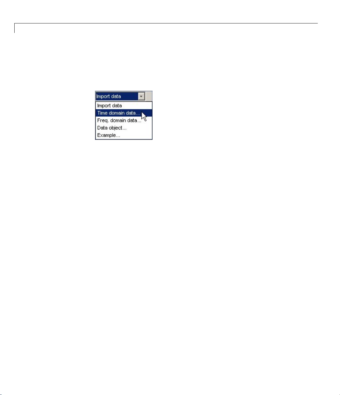
1 In the System Identification Tool GUI, select Import data > Time

domain data. This action opens the Import Data dialog box.

2 Specify the following options:

• Input —Enter

• Output —Enter

• Data name — Change the default name to

u2 as the name of the input variable.

y2 as the name of the output variable.

data. Thisnamelabelsthe

data in the System Identification Tool GUI after the impo rt operation is completed.

• Starting time —Enter

0 as the starting time. This value designates

thestartingvalueofthetimeaxisontimeplots.

• Sampling interval —Enter

0.08 asthetimebetweensuccessive

samples in seconds. This value is the actual sampling interval in the experiment.

4-6

Preparing Data for System Identification

The Import Data dialog box now resembles the following figure.

4-7

4 Tutorial – Identifying Linear Models Using the GUI

3 In the Data Information area, click More to expand the dialog box. Enter

the settings shown in the following figure.

4-8

Input Properties

Preparing Data for System Identification

• InterSample — Accept the default

zoh (zero-order hold) to indicate

that the input signal was piecewise-constant between samples during data acquisition. This setting specifies the behavior of the input signals between samples whe n you transform the resulting models between discrete-time and continuous-time representations.

• Period — Accept the default

inf to specify a nonperiodic input.

Note For a pe riodic input, enter the whole number of periods of the input signal in your experiment.

Channel Names

• Input —Enter

power.

Tip Naming channels helps you to identify data in plots. For multivariable input and output signals, you can specify the names of individual Input and Output channels, separated by commas.

• Output —Entertemperature.

Physical Units of V ariables

• Input —Enter

W for pow er units.

Tip When you have multiple inputs and outputs, enter a comma-separated list of Input and Output units corresponding to each channel.

• Output —Enter^oC for temperature units.

Notes — Enter comments about the experiment or the data. For

example, you might enter the experiment name, date, and a description

4-9

4 Tutorial – Identifying Linear Models Using the GUI

of experimental co nditions. When you estimate models from this data, these models inhe rit your data notes.

4 Click Import to add the icon named data to the System Identification

Tool GUI.

4-10

5 Click Close to close the Import Data dialog box.

Plotting and Processing Data

In this portion of the tutorial, you evaluate the data and process it for system identification. Y ou learn how to:

• Plot the data.

• Subtract the mean values of the input and the output to remove offsets.

• Split the data into two parts. You use one part of the data for model

estimation, and the other part of the data for model validation.

The reason you subtract the mean values from each signal is because, typically, you build linear models that describe the responses for deviations from a physical equilibrium. With steady-state data, it is reasonable to assume that the mean levels of the signals correspond to such an equilibrium. Thus, you can seek models around zero without modeling the absolute equilibrium levels in physical units.

Preparing Data for System Identification

You must have already imported data into the System Identification Tool, as described in “Importing Data Arrays into the System Identification Tool” on page 4-5.

To plot and process the data:

1 In the System Identification Tool GUI, select the Time plot check box to

open the Time Plot. If the plot window is empty, click the data icon in the System Identification Tool GUI.

op axes show the output d ata (temperature), and the bottom axes

The t

the input data (power). Both the input and the output data have

show

ero mean values.

nonz

4-11

4 Tutorial – Identifying Linear Models Using the GUI

2 In the System Identification Tool GUI, select <--Preprocess > Remove

means to subtract the mean input value from the input data and the mean output value from the output data.

4-12

Preparing Data for System Identification

This action adds a new data set to the System Identification Tool GUI with the default name

datad (the suffix d means detrend), and updates the

Time Plot window to display both the original and the detrended data. The detrended data has a zero mean value.

4-13

4 Tutorial – Identifying Linear Models Using the GUI

3 In the System Identification Tool GUI, drag the datad data set to the

Working Data rectangle. This action specifies the detrended data to be used for estimating models.

4-14

4 Select <--Preprocess > Select range to open the Select Range window.

In this window, you can split the data into two parts and specify the first part for model estimation, and the second part for model validation, as described in the following steps.

Preparing Data for System Identification

5 In the Select Range window, change the Samples field to select the first

500 samples, as follows:

1 500

Tip You can also select data samples using the mouse by clicking and dragging a rectangular region on the plot. If you select samples on the input-channel axes, the corresponding region is also selected on the output-channel axes.

4-15

4 Tutorial – Identifying Linear Models Using the GUI

6 In the Data name field, type the name estima te,andclickInsert.This

action adds a new data set to the System Identification Tool GUI to be used for model estimation.

7 In the Select Range window, change the Samples field to select the last

500 samples, as follows:

501 1000

4-16

Preparing Data for System Identification

8 In the Data name field, type the name valida te,andclickInsert.This

action adds a new data set to the System Identification Tool GUI to be used for model validatio n.

9 Drag and drop estimate to the Working Data rectangle, and drag and

drop

validate to the Validation Data rectangle so that the System

Identification Tool GUI resembles the following figure.

4-17

4 Tutorial – Identifying Linear Models Using the GUI

10 To get information about a data set, right-click its icon. For example,

right-click the

estimate data set to open the Data/model Info dialog box.

4-18

Preparing Data for System Identification

IntheData/modelInfodialogbox,youcan perform the following actions:

• Change the name of the data set in the Data name field.

• Change the color of the data icon by changing the RGB values (relative

amounts of red, green, and blue). Each value is between example,

[1,0,0] indicates that only red is present, and no green and

0 and 1.For

blue are mixed into the o verall color.

• In the noneditable area, view the total number of samples, the sampling

interval, and the output and input channel names and units.

• In the editable Diary And Notes area, view or edit the actions you

performed on this data set. The actions are translated into commands equivalent to your GUI operations. For example, as shown in the Data/model Info: estimate window, the

estimate data set is a result of

importing the data, detrending the mean values, and selecting the first 500 samples o f the data:

% Import data datad = detrend(data,0) estimate = datad([1:500])

For m ore information about these and other toolbox commands, see the reference page corresponding to each command.

Tip As an alternative shortcut, you can select Preprocess > Quick start from the System Identification Tool GUI to perform all of the data processing stepsinthistutorial.

Learn More

For information about supported data processing operations, such as resampling and filtering the data, see the System Identification Toolbox User’s Guide.

4-19

4 Tutorial – Identifying Linear Models Using the GUI

Saving the GUI Session

After you process the data, as describedin“PlottingandProcessingData” on page 4-10, you can delete any data sets in the window that you do not need for estimation and validation, and save your session. You can open this session later and use it as a starting point for model estimation and validation without repeating these preparatory steps.

You must have already processed the data into the System Identification Tool, as described in “Plotting and Processing Data” on page 4-10.

To delete specific data sets from a session and save the session:

1 In the Sy s tem Identification Tool GUI, drag and drop the data data set

into the Trash.

2 Drag and drop the datad data set into the Trash.

4-20

Note Moving items to the Trash does not delete them. To permanently delete items, select Options > Empty trash in the System Identification Tool GUI.

Saving the GUI Session

The following figure shows the System Identification Tool GUI after moving the items to the Trash.

3 Drag and drop the estimate and validate data sets to fill the empty

rectangles, as shown in the following figure.

4 Select File > Save session as to open the Save Session dialog box, and

browse to the folder where you want to save the session file.

5 In the File name field, type the name of the session dryer2_prep_data,

and click Save. The resulting file has a

.sid extension.

4-21

4 Tutorial – Identifying Linear Models Using the GUI

Tip You can open a saved se ssion when starting the System Identification

Tool. For example, you can type the following command in the MATLAB Command Window:

ident('dryer2_prep_data')

For more information about managing sessions, see the topics on working with the System Identification Tool GUI in the System Identification Toolbox User’s Guide.

4-22

Estimating Linear Models Using Quick Start

In this section...

“How to Estimate Linear Models Using Quick Start” on page 4-23

“Types of Quick Start Linear Models” o n page 4-24

“Validating the Quick Start Models” on page 4-25

How to Estimate Linear Models Using Quick Start

You can use the Quick Start feature in the System Identification Toolbox to estimate linear models. Quick Start might produce the final linear models you decide to use, or provide you with information required to configure the estimation of accurate parametric models, such as time constants, input delays, and resonant frequencies.

You must have already processed the data for estimation, as described in “Plotting and Processing Data” on page 4-10.

To identify linear models:

• In the System Identification Tool GUI, select E stimate > Quick start.

This action generates plots of step response, frequency-response, and the output of state-space and polynomial models. For more information about these plots, see “Validating the Quick Start Models” on page 4-25.

4-23

4 Tutorial – Identifying Linear Models Using the GUI

Types of Quick Start Linear Models

Quick Start estimates the following four types of models and adds the following to the System Identification Tool GUI w ith default names:

4-24

•

imp — Step response over a period of time using the impulse algorithm.

spad — Frequency response over a range of frequencies using the spa

•

algorithm. The frequency response is the Fourier transform of the impulse response of a linear system.

By default, the model is evaluated at 128 frequency values, ranging from 0 to the Nyquist frequency.

Estimating Linear Models Using Quick Start

• arxqs — Fourth-order autoregressive (ARX) model using the arx algorithm.

This model is parametric and has the following structure:

yt a yt a yt n

() ( ) ( )

+−++ −=

1 …

ut n b ut n

() (

−++ −−

knbk

na a

… b

nnet

++1) ( )

y(t) representstheoutputattimet, u(t) represents the input at time t, n

is the number of poles, nbis the number of b parameters (equal to the

number of zeros plus 1), n

is the number of samp le s before the input affects

output of the system (called the delay or dead time of the model), and e(t) is the white-noise disturbance. The System Identification Toolbox product

estimates the parameters

…

and

…

using the input and output

data from the estimation data set.

arxqs, n

n4s3 — State-space modelcalculatedusingn4sid.Thealgorithm

•

=4, and nkis estimated from the step response model imp.

a=nb

automatically selects the model order (in this case, 3).

This model is parametric and has the following structure:

xt Axt But Ket

( ) () () ()

+= + +

yt Cxt Dut et

() () () ()

=+ +

y(t) represents the output at time t, u(t) represents the input at time t, x is the state vector, and e(t) is the white-noise disturbance. The System Identification Toolbox product estimates the state-space matrices A, B, C, D,andK.

Validating the Quick Start Models

Quick Start generates the following plots duri ng model estimation to help you validate the quality of the models:

• Step-response plot

• Frequency-response plot

• Model-output plot

4-25

4 Tutorial – Identifying Linear Models Using the GUI

You must have already estimated models using Qu ick Start to generate these plots, as described in “How to Estimate Linear Models Using Quick Start” on page 4-23.

Step-Response Plot

The following step-response plot shows agreement among the different model structures and the measured data, which means that all of these structures have similar dynamics.

Tip If you closed the plot window, select the Transient resp check box to reopen this window. If the plot is empty, click the model icons in the System Identification Tool window to display the mode ls on the plot.

4-26

Step Response for imp, arxqs, and n4s3

Estimating Linear Models Using Quick Start

Tip You can use the step-response plot to estimate the dead time of linear systems. Fo r example, the previous step-response plot shows a time delay of about 0.25 s before the system responds to the input. This response delay, or dead time,isapproximatelyequaltoabout three samples because the sampling interval is

0.08 s for this data set.

Frequency-Response Plot

The following frequency-response plot shows agreement among the different model structures and the measured data, which means that all of these structures have similar dynamics.

Tip If you closed this plot window, select the Frequency resp check box to reopen this window. If the plot is empty, click the model icons in the System Identification Tool window to display the mode ls on the plot.

Frequency Response for Models spad, arxqs, and n4s3

4-27

4 Tutorial – Identifying Linear Models Using the GUI

Note The frequency-response plot does not include the impulse-response

model,

Model-Output Plot

The Model Output window shows agreement among the different model structures and the measured output in the validation data.

Tip If you closed the Model Output window, select the Model output check box to reopen this window. If the plot is empty, click the model icons in the System Identification Tool window to display the models on the plot.

imp.

4-28

Measured Output and Model Output for Mo dels imp, arxqs, and n4s3

Estimating Linear Models Using Quick Start

The model-output plot shows the model response to the input in the validation data. The fit values for each model are summarized in the Best Fits area of the Model Output window. The models in the Best Fits list are ordered from best at the top to worst at the bottom. The fit between the two curves is computed such that 100 means a perfect fit, and 0 indicates a poor fit (that is, the model output has the same fit to the measured output as the mean of the measured output).

In this example, the output of the models matches the validation data output, which indicates that the models seem to capture the main system dynamics and that linear modeling is sufficient.

Tip To compare predicted model output instead of simulated output, select this option from the Options menu in the Model Output window.

4-29

4 Tutorial – Identifying Linear Models Using the GUI

Estimating Accurate Linear Models

In this section...

“Strategy for Estimating Accurate Models” on page 4-30

“Estimating Possible Model Orders” on page 4-30

“Identifying State-Space Models” on page 4-35

“Identifying ARMAX Input-Output Polynomial Models” on page 4-36

“Choosing the Best Model” on page 4-39

Strategy for Estimating Accurate Models

The linear models you estimated in “Estimating Linear Models Using Quick Start” on page 4-23 showed that a linear model sufficiently represents the dynamics of the system.

In this portion of the tutorial, you get accurate parametric models by performing the follow ing tasks:

4-30

1 Identifying initial model orders and delays from your data using a simple,

polynomial model structure (ARX).

2 Exploring more complex model structures with orders and delays close to

the initial values you found.

Theresultingmodelsarediscrete-timemodels.

Tip You can convert a linear discrete-time model to a continuous-time model using the reference page.

d2c command. For more information, see the corresponding

Estimating Possible M odel Orders

To identify black-box models, you must specify the model order. However, how can you tell what model orders to specify for your black-box models? To answer this question, you can estimate simple polynomial (ARX) models for a range of orders and delays and compare the performance of these models. You

Estimating Accurate Linear Models

choose the orders and delays that correspond to the best model fit as an initial guess for more accurate modeling.

About ARX Models

For a single-input/single-output system (SISO), the ARX model structure is:

yt a yt a yt n

() ( ) ( )

+−++ −=

y(t) representstheoutputattimet, u(t) represents the input at time t, nais the number of poles, n number of samples before the input affects the system output (called delay or dead time of the model), and e(t) is the white-noise disturbance.

1 …

ut n b ut n

() (

−++ −−

knbk

na a

… b

is the number of zeros plus 1, nkis the input delay—the

nnet

++1) ( )

You specify the model orders n

System Identification Toolbox product estimates the parameters

and

…

from the data.

, nb,andnkto estimate ARX models. The

How to Estimate Model Orders

1 In the System Identification Tool G UI, select Estimate > Linear

parametric models to open the Linear Parametric Models dialog box.

The ARX model is already selected in the Structure list.

…

4-31

4 Tutorial – Identifying Linear Models Using the GUI

2 Edit the Orders field to try all combinations of poles, zeros, and delays,

where each value is from 1 to 10:

[1:10 1:10 1:10]

4-32

Estimating Accurate Linear Models

3 Click Estimate to open the ARX Model Structure Selection window, which

displays the model performance for each combination of model parameters.

You use this plot to select the best-fit model. The horizontal axis is the total number of parameters:

Number of parameters =+nn

The vertical axis, called Unexplained output variance (in %),is the portion of the output not explained by the model—the ARX model prediction error for the number of parameters s ho wn on the horizon tal axis. The prediction error is the sum of the squares of the differences between the validation data output and the model one-step-ahead predicted output.

4-33

4 Tutorial – Identifying Linear Models Using the GUI

Three rectangles are highlighted on the plot in green, blue, and red. Each color indicates a type of best-fit criterion, as follows:

• Red — Best fit minimizes the sum of the squares of the difference

between the validation data output and the model output. This rectangle indicates the ov erall best fit.

• Green — Best fit minimizes Rissanen MDL criterion.

• Blue — Best fit minimizes Akaike AIC criterion.

In this tutorial, the Unexplained output variance (in %) value remains approximately constant for the combined number of parameters from 4 to

20. Such constancy indicates that model performance does not improve at higher orders. Thus, low-order models might fit the data equally well.

Note When you use the same data set for estimation and validation, use the MDL and AIC criteria to select model orders. These criteria compens ate for overfitting that results from using too many parameters. For more information about these criteria, see the

selstruc reference page.

4-34

4 In the ARX Model Structure Selection window, click the red bar

(corresponding to selection inserts n

15 on the horizontal axis), and click Insert.This

=6, nb=9, and nk=2 into the Linear Parametric Models

dialog box a nd performs th e estimation.

This action adds the model

arx692 to the System Identification Tool GUI

and updates the plots to include the response of the model.

Note The default name of the parametric model contains the model type and the number of poles, zeros, and delays. For example, model with n

5 In the ARX Model Structure Selection window, click the third bar

corresponding to

=6, nb=9, and a delay of two samples.

4 parameters on the horizontal axis (the lowest order that

arx692 is an ARX

still gives a good fit), and click Insert.

Estimating Accurate Linear Models

• This selection inserts na=2, nb=2, and nk=3 (a delay of three samples) into

the Linear Parametric Models dialog box and performs the estimation.

• The model

arx223 is added to the System Identification Tool GUI and

theplotsareupdatedtoincludeitsresponseandoutput.

6 Click Close to close the ARX Model Structure Selection window.

Identifying State-Space Models

By estimating ARX models for different order combinations, as described in “Estimating Possible Mod el Orders” on page 4-30, you identified the n umber of poles, zero s, and delays that provide a good starting point for systematically exploring different models.

The ove rall best fit for this system corresponds to a model with six poles, nine zeros, and a delay of two samples. It also showed that a low-order model with

=2 (two poles), nb=2 (one zero), and nk=3 (input-output delay) also provides

a goo d fit. Thus, you should explore model orders close to these values.

In this po rtion of the tutorial, you estimate a state-space model.

About State-Space Models

The general state-space model structure (innovation form) is:

xt Axt But Ket

( ) () () ()

+= + +

yt Cxt Dut et

() () () ()

=+ +

y(t) represents the output at time t, u(t) represents the input at time t, x(t) is the state vector at time t,ande(t) is the white-noise disturbance.

You must specify a single integer as the model order (dimension of the state vector) to estimate a state-space model. By default, the delay equals

1.The

System Identification Toolbox product estimates the state-space matrices A, B, C, D,andK from the data.

The state-space model structure is a good choice for quick estimation because it requires that you specify only two parameters to get started: number of poles (the size of the A matrix) and

nk is the delay.

n is the

4-35

4 Tutorial – Identifying Linear Models Using the GUI

How to Estimate State-Space Models

1 In the System Identification Tool G UI, select Estimate > Linear

parametric models to open the Linear Parametric Models dialog box.

2 From the Structure list, select State Space: n [nk].

3 In the Orders field, type 6 to create a sixth-order state-space model.

This choice is based on the fact that the best-fit ARX model has six poles.

Tip Although this tutorial estimates a sixth-order state-space model, you might want to explore whether a lower-order model adequately represents the system dynamics.

4 Click Estimate to add a state-space model called n4s6 to the System

Identification Tool GUI.

4-36

Tip If you closed the Model Output window, you can regenerate it by selecting the Model output check box in the System Identification Tool GUI. If the new model does not appear on the plot, click the model icon in the System Identification Tool GUI to make the model active.

Learn More

To learn more about identifying state-space models, see the corresponding topic in the System Identification Toolbox User’s Guide.

Identifying ARMAX Input-Output Polynomial Models

The ove rall best fit for this system corresponds to a model with six poles, nine zeros, and a delay of two samples. It also showed that a low-order model with

Estimating Accurate Linear Models

na=2 (two poles), nb=2 (one zero), and nk=3 also provides a good fit. Thus, you

should explore model orders close to these values.

In this portion of the tutorial, you estimate an ARMAX input-output polynomial model.

About ARMAX Models

For a single-input/single-output system (SISO), the ARMAX polynomial model structure is:

yt a yt a yt n

() ( ) ( )

+−++ −=

et c et c et n

y(t) represents the output at time t, u(t) represents the input at time t, nais thenumberofpolesforthedynamicmodel,n is the number of poles for the disturbance m odel, nkis the number of samples before the input affects output of the system (called the delay or dead time of the model), and e(t) is the white-noise disturbance.

1 …

ut n b ut n

() (

−++ −−

() ( ) ( ) …

knbk

+−++ −

… b

na a

nc c

)

is the number of zeros plus 1, n

Note The ARMAX model is more flexible than the ARX model because the ARMAX structure contains an extra polynomial to model the additive disturbance.

You must specify the model orders to estimate ARMAX models. The System

…

Identification Toolbox product estimates the model parameters

…

,and

…

from the data.

How to Estimate ARMAX Models

1 In the System Identification Tool G UI, select Estimate > Linear

parametric models to open the Linear Parametric Models dialog box.

2 From the Structure list, select ARMAX: [na nb nc nk] to estimate an

ARMAX model.

4-37

4 Tutorial – Identifying Linear Models Using the GUI

3 In the Orders field, set the orders na, nb, nc,andnk to the following values:

2222

The model name in the Name field is amx2222,bydefault.

4 Click Estimate to add the ARMAX model to the System Identification

Tool GUI.

5 Repeat steps 3 and 4 using higher Orders 3322. These orders result in

a model that fits the data almost as well as the higher order ARX model

arx692.

4-38

Learn More

To learn more about identifying input-output polynomial models, such as ARMAX, see the corresponding topic in the System Identification Toolbox User’s Guide.

Estimating Accurate Linear Models

Choosing the Bes

You can compare m

You must have al Accurate Linea

Summary of Models

The followin includes all on page 4-30.

g figure shows the System Identification Tool GUI, which

of the estimated models in “Estimating Accurate Linear Models”

odels to choose the model with the best performance.

ready estimated the models, as described in “Estimating

r Models” on page 4-30.

tModel

Examining the Model Output

If you closed the Model Output plot, you can regenerate it by selecting the Model output check box in the System Identification Tool GUI. If the model does not appear on the plot, click the model icon in the System Identification Tool GUI to display it on plots.

Examine the model-output plot to see how well the model output matches the measured output in the validation data set. A good model is the simplest

4-39

4 Tutorial – Identifying Linear Models Using the GUI

model that best describes the dynamics and successfully simulates or predicts the output for different inputs.

Models are listed by name in the Best Fits area of the Model Output plot. The highest-order model you created, simpler model

amx3322.

arx692, fits the data as well as the

4-40

Tip To validate your models using a different data set, you can d rag and drop this data set into the Validation Data rectangle in the System Identification Tool GUI. If you transform validation data into the frequency domain, the model-output plot updates to show the model comparison in the frequency domain.

Estimating Accurate Linear Models

To get a closer look at how well these models fit the data, magnify a portion of the pl ot by cli ck ing and dragging a rectangle around the region of interest, as shown in the following figure.

4-41

4 Tutorial – Identifying Linear Models Using the GUI

Releasing the mouse magnifies this region and shows that the output of all models matches the validation data well.

4-42

Viewing Model Parameters

In this section...

“Viewing Model Para m ete r Values” on page 4-43

“Viewing Parameter Uncertainties” on page 4-46

Viewing Model Parameter Values

You can view the numerical parameter values for each estimated model.

You must have already estimated the models, as described in “Estimating Accurate Linear Models” on page 4-30.

Viewing Model Parameters

To view the parameter v alues of the m odel in the System I d entification T ool GUI. The Data/model Info dialog box opens.

amx3322, right-click the model icon

4-43

4 Tutorial – Identifying Linear Models Using the GUI

4-44

The none parame

ditable area of the Data/model In fo dialog box lists the following

ter values:

A(q) = 1 - 1.508q^-1 + 0.7291q^-2 - 0.1219q^-3 B(q) = 0.004257q^-2 + 0.06201q^-3 + 0.02643q^-4 C(q) = 1 - 0.5835q^-1 + 0.2588q^-2

Viewing Model Parameters

These parameter values correspond to the following difference equation for your system:

yt yt yt yt() . ( ) . ( ) . ( )

−−+ −− −=1 508 1 0 7291 2 0 1219 3

0 004257 uut ut ut

et et

() . (

−−

(). (). ()

−+ −+ −+

2 0 06201 3 0 02643 4

0 5835 11 0 2588 2). ( )+−et

Note The coefficient of u(t-2) is not significantly different from zero. T h is lack of difference explains why delay values of both

2 and 3 give good results.

Parameter values appear in the following format:

nb nk

−−

Aq aq a q

()

=+ + +

Bq bq b q

()

=++

Cq cq

()

…

−−−+

…

−−−

… cq

The parameters appear in the ARMAX model structure, as follows:

Aqyt Bqut Cqet()() ()() ()()=+

which corresponds to this general difference e quation:

yt a yt a yt n

() ( ) ( )

+−++ −=

et c et c et n

1 …

ut n b ut n

() (

−++ −−

() ( ) ( ) …

knbk

+−++ −

… b

na a

nc c

)

y(t) represents the output at time t, u(t) represents the input at time t, nais thenumberofpolesforthedynamicmodel,n

is the number of zeros plus 1, n

is the number of poles for the disturbance m odel, nkis the number of samples before the input affects output of the system (called the delay or dead time of the model), and e(t) is the white-noise disturbance.

4-45

4 Tutorial – Identifying Linear Models Using the GUI

Viewing Parameter Uncertainties

You can view parameter uncertainties of estimated models.

You must have already estimated the models, as described in “Estimating Accurate Linear Models” on page 4-30.

To view parameter uncertainties, click Present intheData/modelInfodialog box, and view the model information in the MATLAB Command Window.

A(q) = 1 - 1.508(+-0.05919)q^-1

+ 0.7291(+-0.08734)q^-2

- 0.1219 (+-0.03424)q^-3

B(q) = 0.004257(+-0.001563)q^-2

+ 0.06201(+-0.002409)q^-3 + 0.02643(+-0.005633)q^-4

C(q) = 1 - 0.5835(+-0.07189)q^-1

+ 0.2588(+-0.05253)q^-2

The 1-standard-deviation uncertainty for the model parameters is in parentheses next to each parameter value.

4-46

Mathworks SYSTEM IDENTIFICATION TOOLBOX 7 Installation Guide

Specifications and Main Features

Frequently Asked Questions

User Manual

About the Developers

Product O verview

Why Use This Toolbox?

Related Products

Documentation

About System Identification

What Is System Identification?

About Dynamic Systems and Models

What Is a Dynam ic Model?

Continuous-Time Dynamic Model Example

Discrete-Time Dynamic Model Example

System Identification Requires Measured Data

Why Does System Identification Require Data?

Time Domain Data

Frequency Domain Data

Data Quality Requirements

Data Representation in This Toolbox

Building Models from Data

System Identification Requires a Model Structure

Black-Box Modeling

Selecting Black-Box Model Structure and Order

Grey-Box Modeling

Evaluating Model Quality

How to Evaluate and Improve Model Quality

Comparing Model Response to Measured Response

Analyzing Residuals

Analyzing Model Uncertainty

Learn More

UsingThisProduct

When to Use the GUI Versus the Command Line

Starting This Toolbox

Steps for Using This Toolbox

Commands for Model Estimation

Commands for Constructing and Estimating Models

Tutorials to Help You Get Started

Tutorial – Identifying Linear Models Using the GUI

About This Tutorial

Objectives

Data Description

Preparing Data for System Identification

Loading Data into the MATLAB Workspace

Opening the System Identification Tool GUI

Plotting and Processing Data

Learn More

Saving the GUI Session

Estimating Linear Models Using Quick Start

How to Estimate Linear Models Using Quick Start

Types of Quick Start Linear Models

Validating the Quick Start Models

Step-Response Plot

Frequency-Response Plot

Model-Output Plot

Estimating Accurate Linear Models

Strategy for Estimating Accurate Models

Estimating Possible M odel Orders

About ARX Models

How to Estimate Model Orders

Identifying State-Space Models

About State-Space Models

How to Estimate State-Space Models

Learn More

Identifying ARMAX Input-Output Polynomial Models

About ARMAX Models

How to Estimate ARMAX Models

Learn More

Summary of Models

Examining the Model Output

Viewing Model Parameters

Viewing Model Parameter Values

Viewing Parameter Uncertainties