

Page 1

Symbolic Math Tool
User’s Guide
box™ 5
Page 2

How to Contact The MathWorks
www.mathworks.
comp.soft-sys.matlab Newsgroup
www.mathworks.com/contact_TS.html T echnical Support
suggest@mathworks.com Product enhancement suggestions
bugs@mathwo
doc@mathworks.com Documentation error reports
service@mathworks.com Order status, license renewals, passcodes
info@mathwo
com
rks.com
rks.com
Web
Bug reports
Sales, prici
ng, and general information
508-647-7000 (Phone)
508-647-7001 (Fax)
The MathWorks, Inc.
3 Apple Hill Drive
Natick, MA 01760-2098
For contact information about worldwide offices, see the MathWorks Web site.
Symbolic Math Toolbox™ User’s Guide
© COPYRIGHT 1993–20 10 by The MathWorks, Inc.
The software described in this document is furnished under a license agreement. The software may be used
or copied only under the terms of the license agreement. No part of this manual may be photocopied or
reproduced in any form without prior written consent from The MathW orks, Inc.
FEDERAL ACQUISITION: This provision applies to all acquisitions of the Program and Documentation
by, for, or through the federal government of the United States. By accepting delivery of the Program
or Documentation, the government hereby agrees that this software or documentation qualifies as
commercial computer software or commercial computer software documentation as such terms are used
or defined in FAR 12.212, DFARS Part 227.72, and DFARS 252.227-7014. Accordingly, the terms and
conditions of this Agreement and only those rights specified in this Agreement, shall pertain to and govern
theuse,modification,reproduction,release,performance,display,anddisclosureoftheProgramand
Documentation by the federal government (or other entity acquiring for or through the federal government)
and shall supersede any conflicting contractual terms or conditions. If this License fails to meet the
government’s needs or is inconsistent in any respect with federal procurement law, the government agrees
to return the Program and Docu mentation, unused, to The MathWorks, Inc.
Trademarks
MATLAB and Simulink are registered trademarks of The MathWorks, Inc. See
www.mathworks.com/trademarks for a list of additional trademarks. Other product or brand
names may be trademarks or registered trademarks of their respective holders.
Patents
The MathWorks products are protected by one or more U.S. patents. Please see
www.mathworks.com/patents for more information.
Page 3

Revision History
August 1993 First printing
October 1994 Second printing
May 1997 Third printing Revised for Version 2
May 2000 Fourth printing Minor changes
June 2001 Fifth printing Minor changes
July 2002 Online only Revised for Version 2.1.3 (Release 13)
October 2002 Online only Revised for Version 3.0.1
December 2002 Sixth printing
June 2004 Seventh printing Revised for Version 3.1 (Release 14)
October 2004 Online only Revised for Version 3.1.1 (Release 14SP1)
March 2005 Online only Revised for Version 3.1.2 (Release 14SP2)
September 2005 Online only Revised for Version 3.1.3 (Release 14SP3)
March 2006 Online only Revised for Version 3.1.4 (Release 2006a)
September 2006 Online only Revised for Version 3.1.5 (Release 2006b)
March 2007 Online only Revised for Version 3.2 (Release 2007a)
September 2007 Online only Revised for Version 3.2.2 (Release 2007b)
March 2008 Online only Revised for Version 3.2.3 (Release 2008a)
October 2008 Online only Revised for Version 5.0 (Release 2008a+)
October 2008 Online only Revised for Version 5.1 (Release 2008b)
November 2008 Online only Revised for Version 4.9 (Release 2007b+)
March 2009 Online only Revised for Version 5.2 (Release 2009a)
September 2009 Online only Revised for Version 5.3 (Release 2009b)
March 2010 Online only Revised for Version 5.4 (Release 2010a)
Page 4

Page 5

Introduction
1
Product Overview ................................. 1-2
Contents
Accessing Symbolic Math Toolbox Functionality
Key Features
Working from MATLAB
Working from MuPAD
..................................... 1-3
............................ 1-3
............................. 1-3
Getting Started
2
Symbolic Objects .................................. 2-2
Overview
Symbolic Variables
Symbolic Numbers
Creating Symbolic Variables and Expressions
Creating Symbolic Variables
Creating Symbolic Expressions
Creating Symbolic Objects with Identical Names
Creating a Matrix of Symbolic Variables
Creating a Matrix of Symbolic Numbers
Finding Symbolic V a r i ab les in Expressions and
Matrices
........................................ 2-2
................................ 2-2
................................ 2-3
........ 2-6
........................ 2-6
...................... 2-7
........ 2-8
............... 2-9
............... 2-10
....................................... 2-10
..... 1-3
Performing Symbolic Computations
Simplifying Symbolic Expressions
Substituting in Symbolic Expressions
Estimating the Precision of Numeric to Symbo lic
Conversions
Differentiating Sy m bo lic Expressions
Integrating Symbolic Expressions
.................................... 2-17
................. 2-12
.................... 2-12
................. 2-14
................. 2-19
.................... 2-21
v
Page 6

Solving Equations ................................. 2-23
Finding a Default Symbolic Variable
Creating Plots of Symbolic Functions
.................. 2-25
................. 2-25
Assumptions for Symbolic Objects
Default Assumption
Setting Assumptions for Symbolic Variables
Deleting Symbolic Objects and Their Assumptions
............................... 2-30
.................. 2-30
........... 2-30
...... 2-31
Using Symbolic Math Toolbox Software
3
Calculus .......................................... 3-2
Differentiation
Limits
Integration
Symbolic Summation
Taylor Series
Calculus Example
Extended Calculus Example
Simplifications and Substitutions
Simplifications
Substitutions
........................................... 3-8
.................................... 3-2
....................................... 3-12
.............................. 3-19
..................................... 3-20
................................. 3-22
......................... 3-30
................... 3-42
.................................... 3-42
..................................... 3-53
vi Contents
Variable-Precision Arithmetic
Overview
Example: Using the Different Kinds of Arithmetic
Another Example Using Different Kinds of Arith metic
Linear Algebra
Basic Alg ebraic Operations
Linear Algebraic Operations
Eigenvalues
Jordan Canonical Form
Singular Value Decomposition
Eigenvalue Trajectories
........................................ 3-60
.................................... 3-66
...................................... 3-72
............................ 3-77
............................ 3-82
...................... 3-60
......................... 3-66
........................ 3-67
....................... 3-79
...... 3-61
... 3-64
Page 7

Solving Equation s ................................. 3-93
Solving Algebraic Equations
Several Algebraic Equations
Single Differential Equation
Several Differential Equat ions
......................... 3-93
........................ 3-94
......................... 3-97
....................... 3-100
Integral Transforms and Z-Transforms
The Fourier and Inverse Fourier Transforms
The Laplace and Inverse Laplace Transforms
The Z– and Inverse Z–transforms
Special Fu nctions of App lied Mathematics
Numerical Evaluation of Special Functions Using mfun
Syntax and Definitions of mfun Special Functions
Diffraction Example
Generating Code from Symbolic Expressions
Generating C or Fortran Code
Generating MATLAB Functions
Generating Em bedded MATLAB F unction Blocks
Generating Simscape Equations
............................... 3-125
.................... 3-115
....................... 3-128
..................... 3-129
..................... 3-139
.............. 3-102
........... 3-102
.......... 3-109
........... 3-119
....... 3-120
......... 3-128
....... 3-134
MuPAD in Symbolic Math Toolbox
4
Understanding MuP AD ............................ 4-2
Introduction to MuPAD
The MATLAB Workspace and MuPAD Engines
Introductory Example Using a MuPAD Notebook from
MATLAB
...................................... 4-3
............................ 4-2
......... 4-2
.. 3-119
MuPAD for MATLAB Users
Getting Help for MuPAD
Launching, Opening, and Saving MuPAD Notebooks
Opening Recent Files and Other MuPAD Interfaces
Calculating in a MuPAD Notebook
Differences Between MATLAB and MuPAD Syntax
......................... 4-10
........................... 4-10
................... 4-15
.... 4-12
..... 4-13
..... 4-21
vii
Page 8

Integration of MuPAD and MATLAB ................ 4-25
Copying Variables and Expressions Between the MATLAB
Workspace and MuPAD Notebooks
Calling MuPAD Functions at the MATLAB Command
Line
.......................................... 4-28
Clearing Assumptions and Resetting the Symbolic
Engine
........................................ 4-31
................. 4-25
Function Reference
5
Calculus .......................................... 5-2
Linear Algebra
Simplification
Solution of Equations
Variable Precision Arithmetic
Arithmetic Operations
Special Fu nctions
MuPAD
Pedagogical and Graphical Applications
Conversions
Basic Operations
........................................... 5-5
.................................... 5-2
..................................... 5-3
.............................. 5-4
...................... 5-4
............................. 5-4
.................................. 5-5
....................................... 5-7
.................................. 5-8
............. 5-6
viii Contents
Integral and Z-Transforms
......................... 5-9
Page 9

6
Functions — Alphabetical List
Index
ix
Page 10

x Contents
Page 11

Introduction
• “Product Overview” on page 1-2
• “Accessing Symbolic Math Toolbox Functionality” on page 1-3
1
Page 12

1 Introduction
Product Overview
Symbolic Math Toolbox™ softw are lets you to perform symbolic computations
within the MATLAB
manipulating symbolic math expressions and performing variable-precision
arithmetic. The toolbox contains hundreds of symbolic functions that leverage
the MuPAD
• Differentiation
• Integration
• Linear algebraic operations
• Simplification
• Transforms
• Variable-precision arithmetic
• Equation solving
Symbolic Math Toolbox software also includes the MuPAD language, which
is optimized for handling and operating on symbolic math expressions. In
addition to covering common mathematical tasks, the libraries of MuPAD
functions cover specialized areas such as number theory and combinatorics.
You can extend the built-in functionality by writing custom symbolic functions
and libraries in the MuPAD language.
®
engine for a broad range of mathematical tasks such as:
®
numeric en vironment. It provides tools for solving and
1-2
Page 13

Accessing Symbolic Math Toolbox™ Func tionality
Accessing Symbolic Math Toolbox Functionality
Key Features
Symbolic Math Toolbox software provides a complete set of tools for symbolic
computing that augments the numeric capabilities of MATLAB. The toolbox
includes extensive symbolic functionality that you can access directly from
the MATLAB command line or from the MuPAD Notebook Interface. You can
extend the functionality available in the toolbox by writing custom symbolic
functions or libraries in the MuPAD language.
Working from MATLAB
You can access the Symbolic Math Toolbox functionality directly from the
MATLAB Command Window. This environment lets you call functions using
familiar MATLAB syntax.
The M A TLAB Help browser presents the documentation that covers working
from the MATLAB Comm and Window. To access the MATLAB Help browser,
you can:
• Select Help > Product Help ,andthenselectSymbolic Math Toolbox
in the left pane
• Enter
If y ou are a new user, begin with Chapter 2, “Getting Started”
doc at theMATLAB command line
Working from MuPAD
Also you can access the Symbolic Math Toolbox functionality from the MuPAD
Notebook Interface using the MuPAD language. The MuPAD Notebook
Interface includes a symbol palette for accessing common MuPAD functions.
All results are displayed in typeset math. You also can convert the results
into MathML and T eX. You can embed graphics, animations, and descriptive
text within your notebook.
An editor, debugger, and other programming utilities provide tools for
authoring custom symbolic functions and libraries in the MuPAD language.
The MuPAD language supports multiple programming styles including
1-3
Page 14

1 Introduction
imperative, functional, and object-oriented programming. The language treats
variables as symbolic by default and is optimized for handling and operating
on symbolic math expressions. You can call functions written in the MuPAD
language from the MATLAB Command Window. For more information see
“Calling MuPAD Functions at the MATLAB Command Line” on page 4-28
The MuPAD Help browser presents documentation covering the MuPAD
Notebook Interface. To access the MuPAD Help browser :
• From the MuPAD Notebook Interface, select Help > Open Help
• From the MATLAB Command Window, enter
If you are a new user of the M uPAD Notebook Interface, read the Getting
Started chapter of the MuPAD documentation.
There is a lso a MuPAD Tutorial PDF file available at
http://www.mathworks.com/access/helpdesk/...
help/pdf_doc/symbolic/mupad_tutorial.pdf
doc(symengine).
.
1-4
Page 15

Getting Started
• “Symbolic Objects” on page 2-2
• “Creating Symbolic Variables and Expressions” on page 2-6
• “Performing Symbolic Computations” on page 2-12
• “Assumptions for Symbolic Objects” on page 2-30
2
Page 16

2 Getting Started
Symbolic Objects
In this section...
“Overview” on page 2-2
“Symbolic Variables” on page 2-2
“Symbolic Numbers” on page 2-3
Overview
Symbolic objects are a special MATLAB data type introduced by the Symbolic
Math Toolbox software. They allow you to perform mathematical operations
in the MATLAB workspace analytically, without calculating numeric
values. You can use symbolic objects toperformawidevarietyofanalytical
computations:
• Differentiation, including partial differentiation
• Definite and indefinite integration
2-2
• Taking limits, including one-sided limits
• Summation, including Taylor series
• Matrix operations
• Solving algebraic and differential equations
• Variable-precision arithmetic
• Integral transforms
Symbolic objects present symbolic variables, symbolic numbers, symbolic
expressions and symbolic matrices.
Symbolic Variables
To declare variables x and y as symbolic objects use the syms comm and:
syms x y
Page 17

Symbolic Objects
You can m anipulate the symbolic objects according to the usual rules of
mathematics. For example:
x+x+y
ans =
2*x + y
You also can create formal symbolic mathematical expressions and symbolic
matrices. See “Creating Symbolic Variables and Expressions” on page 2-6
for more information.
Symbolic Numbers
Symbolic Math Toolbox software also enables you to convert numbers to
symbolic objects. To create a symbolic number, use the
a = sym('2')
If you create a symbolic number with 10 or fewer decimal digits, you can
skip the quotes:
sym command:
a = sym(2)
The following example illustrates the difference between a standard
double-precision MATLAB data and the corresponding symbolic number.
The MATLAB command
sqrt(2)
returns a double-precision floating-point number:
ans =
1.4142
On the other hand, if you calculate a square root of a symbolic number 2:
a = sqrt(sym(2))
you get the precise symbolic result:
a=
2^(1/2)
2-3
Page 18

2 Getting Started
Symbolic results are not indented. Standard MATLAB double-precision
results are indented. The difference in output form shows what type of data is
presented as a result.
To evaluate a symbolic number numerically, use the
double(a)
ans =
1.4142
double command:
You also can create a rational fraction involving symbolic numbers:
sym(2)/sym(5)
ans =
2/5
or more efficiently:
sym(2/5)
ans =
2/5
MATLAB performs arithmetic on symbolic fractions differently than it does
on standard numeric fractions. By default,MATLAB stores all numeric values
as double-precision floating-point data. For example:
2/5 + 1/3
2-4
ans =
0.7333
Ifyouaddthesamefractionsassymbolic objects, MATLAB finds their
common denominator and combines them in the usual procedure for adding
rational numbers:
sym(2/5) + sym(1/3)
ans =
11/15
Page 19

Symbolic Objects
To learn more about symbolic representation of rational and decimal fractions,
see “Estimating the Precision of NumerictoSymbolicConversions”onpage
2-17.
2-5
Page 20

2 Getting Started
Creating Symbolic Variables and Expressions
In this section...
“Creating Symbolic Variables” on page 2-6
“Creating Symbolic Expressions” on page 2-7
“Creating Symbolic Objects with Identical Names” on page 2-8
“Creating a Matrix of Symbolic Variables” on page 2-9
“Creating a Matrix of Symbolic Numbers” on page 2-10
“Finding Symbolic Variables in Expression s and Matrices” on page 2-10
Creating Symbolic Variables
The sym command creates symbolic variables and expressions. For example,
the commands
2-6
x = sym('x');
a = sym('alpha');
create a symbolic variable x with the value x assigned to it in the MATLAB
workspace and a symbolic variable
alternate way to create a s ymbolic object is to use the
syms x;
a = sym('alpha');
You can use sym or syms to create symbolic variables. The syms command:
• Does not use parentheses a nd quotation marks:
• Can create multiple objects with one call
• Serves best for creating individual single and mu ltiple symbolic variables
The
sym command:
a with the value alpha assigned to it. An
syms command:
syms x
Page 21

Creating Symbolic Variables and Expressions
• Requires parentheses and quotation marks: x = sym('x'). When creating
a symbolic number with 10 or fewer decimal digits, you can skip the
quotation marks:
f = sym(5).
• Creates one symbolic object with each call.
• Serves best for creating symbolic numbers and symbolic expressions.
• Serves best for creating symbolic objects in functions and scripts.
Note In Symbolic Math Toolbox, pi is a reserved word.
Creating Symbolic Expressions
Supposeyouwanttouseasymbolicvariabletorepresentthegoldenratio
+15
=
2
The command
rho = sym('(1 + sqrt(5))/2');
achieves this goal. Now you can perform various mathematical operations
on
rho. For example,
f = rho^2 - rho - 1
returns
f=
(5^(1/2)/2 + 1/2)^2 - 5^(1/2)/2 - 3/2
Now suppose you want to study the quadratic function f = ax2+ bx + c.One
approach is to enter the command
f = sym('a*x^2 + b*x + c');
which assigns the symbolic expression ax2+ bx + c to the variable f. However,
in this case, Symbolic Math Toolbox software does not create variables
corresponding to the terms of the expression:
a, b, c,andx.Toperform
2-7
Page 22

2 Getting Started
symbolic math operations on f, you need to create the variables explicitly. A
better alternative is to enter the commands
a = sym('a');
b = sym('b');
c = sym('c');
x = sym('x');
or simply
syms a b c x
Then, enter
f = a*x^2 + b*x + c;
Note To create a symbolic expression that is a constant, you must use the sym
command. Do not use syms command to create a symbolic expression that is a
constant. For example, to create the expression whose value is
sym(5)
. The command f=5does not define f as a symbolic expression.
5,enterf=
2-8
Creating Symbolic Objects w ith Identical Names
If you set a variable equal to a symbolic expression, and then apply the syms
command to the variable, MATLAB software removes the previously defined
expression from the variable. For example,
syms a b;
f=a+b
returns
f=
a+b
If later you enter
syms f;
f
then MATLAB removes the value a+bfrom the expression f:
Page 23

Creating Symbolic Variables and Expressions
f=
f
You can use the syms command to clear variables of definitions that you
previously assigned to them in your MATLAB session. H ow ev er,
syms does
not clear the f ol lo wi n g assumptions of the variables: complex, real, and
positive. These assumptions are stored separately from the symbolic object.
See “Deleting Symbolic Objects and Their Assumptions” on page 2-31 for
more information.
Creating a Matrix of Symbolic Variables
A circulant matrix has the property that each row is obtained from the
previous one by cyclically permuting the entries one step forward. You can
create the symbolic circulant matrix
the commands:
syms a b c;
A=[abc;cab;bca]
A whose elements are a, b,andc,using
A=
[a,b,c]
[c,a,b]
[b,c,a]
Since the matrix A is circulant, the sum of elements over each row and each
column is the same. Find the sum of all the elements of the first row:
sum(A(1,:))
ans =
a+b+c
Check if the sum of the elements of the first row equals the sum of the
elements of the second column:
sum(A(1,:)) == sum(A(:,2))
The sums are equal:
ans =
1
2-9
Page 24

2 Getting Started
From this example, you can see that using symbolic objects is very similar to
using regular MATLAB numeric objects.
Creating a Matrix of Symbolic Numbers
A particularly effective use of sym is to convert a matrix from numeric to
symbolic form. The command
A = hilb(3)
generates the 3-by-3 Hilbert matrix:
A=
1.0000 0.5000 0.3333
0.5000 0.3333 0.2500
0.3333 0.2500 0.2000
By applying sym to A
A = sym(A)
2-10
you can obtain the precise symbolic form of the 3-by-3 Hilbert matrix:
A=
[ 1, 1/2, 1/3]
[ 1/2, 1/3, 1/4]
[ 1/3, 1/4, 1/5]
For more information on numeric to symbolic conversions see “Estimating the
Precision of Numeric to Symbolic Conversions” on page 2-17.
Finding Symbolic Variables in Expressions and Matrices
To determine what symbolic variables are present in an expression, use
the
symvar command. For example, given the symbolic expressions f and
g defined by
syms a b n t x z;
f = x^n;
g = sin(a*t + b);
Page 25

Creating Symbolic Variables and Expressions
you can find the symbolic variables in f by entering:
symvar(f)
ans =
[n,x]
Similarly, you can find the symbolic variables in g by entering:
symvar(g)
ans =
[a,b,t]
2-11
Page 26

2 Getting Started
Performing Symbolic Computations
In this section...
“Simplifying Symbolic Expressions” on page 2-12
“Substituting in Symbolic Expressions” on page 2-14
“Estimating the Precision of Numeric to Symbolic Conversions” on page 2-17
“Differentiating Symbolic Expressions” on page 2-19
“Integrating Symbolic Expressions” on page 2-21
“Solving Equations” on page 2-23
“Finding a Default Symbolic Variable” on page 2-25
“Creating Plots of Symbolic Functions” on page 2-25
Simplifying Symbolic E xpressions
Symbolic Math Toolbox provides a set of simplification functions allowing you
to manipulate an output of a symbolic expression. For example, the following
polynomial of the golden ratio
rho
2-12
rho = sym('(1 + sqrt(5))/2');
f = rho^2 - rho - 1
returns
f=
(5^(1/2)/2 + 1/2)^2 - 5^(1/2)/2 - 3/2
You can simplify this answer by entering
simplify(f)
and get a very short answer:
ans =
0
Page 27

Performing Symbolic Computations
Symbolic simplification is not always so straightforward. There is no universal
simplification function, because the meaning of a simplest representation of
a symbolic expression cannot be defined clearly. Different problems require
different forms of the same mathematical expression. Knowing what form
is more effective for solving your particular problem, you can choose the
appropriate simplification function.
For example, to show the order of a polynomial or symbolically differentiate
or integrate a poly nomial, use the s tandard polynomial form with all the
parenthesis multiplied out and all the similar terms summed up. To rewrite a
polynomial in the standard form, use the
syms x;
f = (x ^2- 1)*(x^4 + x^3 + x^2 + x + 1)*(x^4 - x^3 + x^2 - x + 1);
expand(f)
ans =
x^10 - 1
expand function:
The factor simplification function shows the polynomial roots. If a
polynomial cannot be factored over the rational numbers, the output of the
factor function is the standard polynomial form. For example, to factor the
third-order polynomial, enter:
syms x;
g = x^3 + 6*x^2 + 11*x + 6;
factor(g)
ans =
(x + 3)*(x + 2)*(x + 1)
The nested (Horner) representation of a polynomial is the most e fficient for
numerical evaluations:
syms x;
h = x^5 + x^4 + x^3 + x^2 + x;
horner(h)
ans =
x*(x*(x*(x*(x + 1) + 1) + 1) + 1)
2-13
Page 28

2 Getting Started
For a list of Symbolic Math Toolbox simplificat ion functions, see
“Simplifications” on page 3-42.
Substituting in Symbolic Expressions
subs Command
You can substitute a numeric value for a symbolic variable or replace one
symbolic variable with another using the
substitute the value
syms x;
f = 2*x^2 - 3*x + 1;
enter the command
subs(f, 2)
ans =
3
x = 2 in the symbolic expression
subs command. For example, to
2-14
Substituting in Multivariate Expressions
When your expression contains more than one variable, you can specify
the variable for which you want to make the substitution. For example, to
substitute the value
syms x y;
f = x^2*y + 5*x*sqrt(y);
enter the command
subs(f, x, 3)
ans =
9*y + 15*y^(1/2)
x = 3 in the symbolic expression
Substituting One Symbolic Variable for Another
You also can substitute one symbolic variable for another symbolic variable.
For example to replace the variable
y with the variable x,enter
Page 29

Performing Symbolic Computations
subs(f, y, x)
ans =
x^3 + 5*x^(3/2)
Substituting a Matrix into a Polynomial
You can also substitute a matrix into a symbolic polynomial with numeric
coefficients. There are two ways to substitute a matrix into a polynomial:
element by element and according to matrix multiplication rules.
Element-by-Element Substitution. To substitute a matrix at each element,
use the
subs command:
A=[123;456];
syms x; f = x^3 - 15*x^2 - 24*x + 350;
subs(f,A)
ans =
312 250 170
78 -20 -118
You can do element-by-element substitution for rectangular or square
matrices.
Substitution in a Matrix Sense. If you want to substitute a matrix into
a polynomial using standard matrix multiplication rules, a matrix must be
square. For example, you can substitute the magic square
f:
1 Create the polynomial:
syms x;
f = x^3 - 15*x^2 - 24*x + 350;
2 Create the magic square matrix:
A = magic(3)
A=
816
357
A into a polynomial
2-15
Page 30

2 Getting Started
492
3 Get a row v ector containing the numeric coefficients of the polynomial f:
b = sym2poly(f)
b=
1 -15 -24 350
4 Substitute the magic square matrix A into the polynomial f.MatrixA
replaces all occurrences of x in the polynomial. Theconstanttimesthe
identity matrix
A^3 - 15*A^2 - 24*A + 350*eye(3)
ans =
-1000
0 -10 0
00-10
eye(3) replaces the constant term of f:
2-16
The polyvalm command provides an easy way to obtain the same result:
polyvalm(sym2poly(f),A)
ans =
-1000
0 -10 0
00-10
Substituting the Elements of a Symbolic Matrix
To substitute a set of elements in a symbolic matrix, also use the subs
command. Suppose you want to replace some of the elements of a symbolic
circulant matrix A
syms a b c;
A=[abc;cab;bca]
A=
[a,b,c]
[c,a,b]
[b,c,a]
Page 31

Performing Symbolic Computations
To replace the (2, 1) element of A with beta and the variable b throughout
the matrix with variable
alpha = sym('alpha');
beta = sym('beta');
A(2,1) = beta;
A = subs(A,b,alpha)
alpha,enter
The result is the matrix:
A=
[ a, alpha, c]
[ beta, a, alpha]
[ alpha, c, a]
For more information on the subs command se
Estimating the Precision of Numeric to S
e “Substitutions” on page 3-53.
ymbolic
Conversions
The sym command converts a numeric scal
default, the
sym command returns a rati
expression. For example, you can conve
variable into a symbolic object:
t = 0.1;
sym(t)
ans =
1/10
The technique for converting floating-point numbers is specified by the
optional second argument, which can be
option is
'r' that stands for rational approximation“Converting to Rational
Symbolic Form” on page 2-18.
Converting to Floating-Point Symbolic Form
The 'f' option to sym converts a double-precision floating-point numb er to a
sum of two binary numbers. All values are represented as rational numbers
N*2^e,wheree and N are integers , and N is nonnegative. Fo r example,
ar or matrix to symbolic form. By
onal approximation of a numeric
rt the standard double-precision
'f', 'r', 'e' or 'd'.Thedefault
2-17
Page 32

2 Getting Started
sym(t, 'f')
returns the symbolic floating-point repre sentation:
ans =
3602879701896397/36028797018963968
Converting to Rational Symbolic Form
If you call sym command with the 'r' option
sym(t, 'r')
you get the results in the rational form:
ans =
1/10
This is the default setting for the sym command. If you call this command
without any option, you get the result in the same rational form:
2-18
sym(t)
ans =
1/10
Converting to Rational Symbolic Form with Machine Precision
If you call the sym command with the option 'e', it returns the rational form
of
t plusthedifferencebetweenthetheoretical rational expression for t and
its actual (machine) floating-point value in terms of
eps (the floating-point
relative accuracy):
sym(t, 'e')
ans =
eps/40 + 1/10
Converting to Decimal Symbolic Form
If you c all the sym command with the option 'd', it returns the decimal
expansion of
t up to the number of significant digits:
Page 33

Performing Symbolic Computations
sym(t, 'd')
ans =
0.10000000000000000555111512312578
By default, the sym(t,'d') command returns a number with 32 significant
digits. To change the number of significant digits, use the
digits(7);
sym(t, 'd')
ans =
0.1
digits command:
Differentiating Symbolic Expressions
With the Symbolic Math Toolbox software, you can find
• Derivatives of single-variable expressions
• Partial derivatives
• Second and higher order derivatives
• Mixed derivatives
For in-depth information on taking symbolic derivatives see “Differentiation”
on page 3-2.
Expressions with One Variable
To diffe rentiate a symbolic expression, u se the diff command. The following
exampleillustrateshowtotakeafirstderivativeofasymbolicexpression:
syms x;
f = sin(x)^2;
diff(f)
ans =
2*cos(x)*sin(x)
2-19
Page 34

2 Getting Started
Partial Derivatives
For multivariable expressions, you can specify the differentiation variable.
If you do not specify any va ri able, MATLAB chooses a default variable by
the proximity to the letter
syms x y;
f = sin(x)^2 + cos(y)^2;
diff(f)
ans =
2*cos(x)*sin(x)
For the complete set of rules MATLAB applies for choosing a default variable,
see “Finding a Default Symbolic Variable” on page 2-25.
x:
To differentiate the symbolic expression
syms x y;
f = sin(x)^2 + cos(y)^2;
diff(f, y)
ans =
(-2)*cos(y)*sin(y)
f with respect to a variable y,enter:
Second Partial and Mixed Derivatives
To take a second derivative of the symbolic expression f with respect to a
variable
You get the same result by taking derivative twice: diff(diff(f, y)).To
take mixed derivatives, use two differentiation comm ands. For example:
y,enter:
syms x y;
f = sin(x)^2 + cos(y)^2;
diff(f, y, 2)
ans =
2*sin(y)^2 - 2*cos(y)^2
syms x y;
f = sin(x)^2 + cos(y)^2;
diff(diff(f, y), x)
2-20
Page 35

ans =
0
Integrating Symbolic Expressions
You can perform symbolic integration including:
• Indefinite and definite integration
• Integration of multivariable expressions
Performing Symbolic Computations
For in-depth information on the
int command including integration with real
and complex parameters, see “Integration” on page 3-12.
Indefinite Integrals of One-Variable Expressions
Suppose you want to integrate a symbolic expression. The first step is to
create the symbolic expression:
syms x;
f = sin(x)^2;
To find the indefinite integral, enter
int(f)
ans =
x/2 - sin(2*x)/4
Indefinite Integrals of Multivariable Expressions
If the expression depends on multiple symbolic variables, you can designate a
variable of integration. If you do not specify any variable, MATLAB chooses a
default variable by the proximity to the letter
syms x y n;
f = x^n + y^n;
int(f)
x:
ans =
x*y^n + (x*x^n)/(n + 1)
2-21
Page 36

2 Getting Started
For the complete set of rules MATLAB applies for choosing a default variable,
see “Finding a Default Symbolic Variable” on page 2-25.
You also can integrate the expression
syms x y n;
f = x^n + y^n;
int(f, y)
ans =
x^n*y + (y*y^n)/(n + 1)
f=x^n+y^nwith respect to y
If the integration variable is n,enter
syms x y n;
f = x^n + y^n;
int(f, n)
ans =
x^n/log(x) + y^n/log(y)
Definite Integrals
To find a definite integral, pass the limits of i n t egration as the final two
arguments of the
syms x y n;
f = x^n + y^n;
int(f, 1, 10)
int function:
2-22
ans =
piecewise([n = -1, log(10) + 9/y],...
[n <> -1, (10*10^n - 1)/(n + 1) + 9*y^n])
IfMATLABCannotFindaClosedFormofanIntegral
If the int function cannot compute an integral, M ATLAB issues a warning
and returns an unresolved integral:
syms x y n;
f = exp(x)^(1/n) + exp(y)^(1/n);
Page 37

Performing Symbolic Computations
int(f, n, 1, 10)
Warning: Explicit integral could not be found.
ans =
int(exp(x)^(1/n) + exp(y)^(1/n), n = 1..10)
Solving Equations
You can solve different types of symbolic equations including:
• Algebraic equations with one symbolic variable
• Algebraic equations with several symbolic variables
• Systems of algebraic equations
For in-depth information on solving symbolic equations including differential
equations, see “Solving Equations” on page 3-93.
Algebraic Equations with One Symbolic Variable
You can find the values of variable x for which the following expression
is equal to zero:
syms x;
solve(x^3 - 6*x^2 + 11*x - 6)
ans =
1
2
3
By default, the solve command assumes that the right-side of the equation is
equal to zero. If you want to solve an equation with a nonzero right part, use
quotation marks around the equation:
syms x;
solve('x^3 - 6*x^2 + 11*x - 5 = 1')
ans =
1
2
2-23
Page 38

2 Getting Started
3
Algebraic Equations with Several Symbolic Variables
If an equation contains several symbolic variables, you can designate a
variable for which this equation should be solved. For example, you can solve
the multivariable equation:
syms x y;
f = 6*x^2 - 6*x^2*y + x*y^2 - x*y + y^3 - y^2;
with respect to a symbolic variable y:
solve(f, y)
ans =
1
2*x
-3*x
2-24
If yo u do not specify any variable, you get the solution of a n equation for the
alphabetically closest to
x variable. For the complete set of rules MATLAB
applies for choosing a default variable see “Finding a Default Symbolic
Variable” on page 2-25.
Systems of Algebraic Equations
Youalsocansolvesystemsofequations. Forexample:
xyz;
syms
, z] = solve('z = 4*x', 'x = y', 'z = x^2 + y^2')
[x, y
x=
0
2
y=
0
2
z=
0
Page 39

Performing Symbolic Computations
8
Finding a Default Symbolic Variable
When performing substitution, differentiation, or integration, if you do not
specify a variable to use, MATLAB uses a default variable. The default
variable is basically the one closest alphabetically to
is chosen as a default variable, use the
symvar(expression, 1) command.
For example:
syms s t;
g=s+t;
symvar(g, 1)
ans =
t
syms sx tx;
g=sx+tx;
symvar(g, 1)
x. To find which variable
ans =
tx
For more information on choosing the default symbolic variable, see the
symvar command.
Creating Plots of Symbolic Functions
You can create different types of graphs including:
• Plots of explicit functions
• Plots of implicit functions
• 3-D parametric plots
• Surface plots
See “Pedagogical and Graphical Applications” on page 5-6 for in-depth
coverage of Symbolic Math Toolbox graphics and visualization tools.
2-25
Page 40

2 Getting Started
Explicit Function Plot
Thesimplestwaytocreateaplotistousetheezplot command:
syms x;
ezplot(x^3 - 6*x^2 + 11*x - 6);
hold on;
The hold on command retains the existing plot allowing you to add new
elements and change the appearance of the plot. For example, now you can
change the names of the axes and add a new title and grid lines. When you
finish working with the current plot, enter the
xlabel('x axis');
ylabel('no name axis');
title('Explicit function: x^3 - 6*x^2 + 11*x - 6');
grid on;
hold off
hold off command:
2-26
Page 41

Performing Symbolic Computations
Implicit Function Plot
You can plot implicitly defined functions. For example, create a plot for the
following implicit function over the domain –1 < x < 1:
syms x y;
f = (x^2 + y^2)^4 - (x^2 - y^2)^2;
ezplot(f, [-1 1]);
hold on;
xlabel('x axis');
ylabel('y axis');
title('Implicit function: f = (x^2 + y^2)^4 - (x^2 - y^2)^2');
grid on;
hold off
2-27
Page 42

2 Getting Started
3-D Plot
3-D graphics is also available in Symbolic Math Toolbox . To create a 3-D plot,
use the
ezplot3 command. For example:
syms t;
ezplot3(t^2*sin(10*t), t^2*cos(10*t), t);
2-28
Page 43

Performing Symbolic Computations
Surface Plot
If you want to create a surface plot, use the ezsurf command. For example, to
plot a paraboloid z=x
syms x y;
ezsurf(x^2 + y^2);
hold on;
zlabel('z');
title('z = x^2 + y^2');
hold off
2+y2
,enter:
2-29
Page 44

2 Getting Started
Assumptions for Symbolic Objects
In this section...
“Default Assumption” on page 2-30
“Setting Assumptions for Symbolic Variables” on page 2-30
“Deleting Symbolic Objects and Their Assumptions” on page 2-31
Default Assumption
In Sym bolic M a th Toolbox, symbolic variables are single complex v ari ab l es by
default. For example, if you declare
syms z
MATLAB assumes z is a com plex variable. You can always check if a symbolic
variable is ass umed to be complex or real by entering
conj(x) == x returns 1, x is a real variable:
z as a symbolic variable:
conj command. If
2-30
z == conj(z)
ans =
0
Setting Assumptions for Symbolic Variables
The sym and syms commands allow you to set up assumptions for symbolic
variables. For example, create the real symbolic variables
positive symbolic variable
x = sym('x', 'real');
y = sym('y', 'real');
z = sym('z', 'positive');
or more efficiently
syms x y real;
syms z positive;
There are two assumptions you can assign to a symbolic object w ithin the sym
command: real and positive. Together with the default complex property of a
z:
x and y and the
Page 45

Assumptions for Symbolic Objects
symbolic variable, it gives you three choices for an assumption for a symbolic
variable: complex, real, and positive.
Deleting Symbolic Objects and Their Assumptions
When you declare x to be real with the command
syms x real
you create a symbolic object x and the assumption that the object is real.
Symbolic objects and their assumptions are stored separately. When you
delete a symbolic object from the MATLAB workspace
clear x
the assumption that x is real stays in symbolic engine. If you declare a new
symbolic variable
getting a default assumption. If later you solve an equation and simplify a n
expression w ith the symbo lic variable
example, the assumption that
no roots:
x later, it inherits the assumption that x is real instead of
x, you could get incomplete results. For
x is real causes the polynomial x
2
+1 to have
syms x real;
clear x;
syms x;
solve(x^2+1)
Warning: Explicit solution could not be found.
> In solve at 81
ans =
[ empty sym ]
The comple x roots of this polynomial disappear because the symbolic variable
x still has the assumption that
x is real stored in the symbolic engine. To
clear the assumption, enter
syms x clear
After you clear the assumption, the symbolic object stays in the MATLAB
workspace. If you want to remove both the symbolic object and its assumption,
use two subsequent commands:
2-31
Page 46

2 Getting Started
1 To clear the assumption, enter
syms x clear
2 To delete the symbolic object, enter
clear x
For more information on clearing symbolic variables, see “Clearing
Assumptions and Resetting the Symbolic Engine” on page 4-31.
2-32
Page 47

Using Symbolic Math Toolbox Software
This section explains how to use Symbolic Math Toolbox software to perform
many common mathematical operations. The section covers the following
topics:
• “Calculus” on page 3-2
• “Simplifications and Substitutions” on page 3-42
3
• “Variable-Precision Arithmetic” o n page 3-60
• “Linear Algebra” on page 3-66
• “Solving Equations” on page 3-93
• “Integral Transforms and Z-Transforms” on page 3-102
• “Special Functions of Applied Mathematics” on page 3-119
• “Generating Code from Symbolic Expressions” on page 3-128
Page 48

3 Using Symbolic Math Toolbox™ Software
Calculus
In this section...
“Differentiation” on page 3-2
“Limits” on page 3-8
“Integration” on page 3-12
“Symbolic Summation” on page 3-19
“Taylor Series” on page 3-20
“Calculus Example” on page 3-22
“Extended Calculus Exam p le” on page 3-30
Differentiation
To illustrate how to take derivatives using Symbolic Math Toolbox software,
first create a symbolic expression:
3-2
syms x
f = sin(5*x)
The command
diff(f)
differentiates f with respect to x:
ans =
5*cos(5*x)
As another example, let
g = exp(x)*cos(x)
where exp(x) denotes ex, and differentiate g:
diff(g)
ans =
exp(x)*cos(x) - exp(x)*sin(x)
Page 49

To take the second derivative of g,enter
diff(g,2)
ans =
-2*exp(x)*sin(x)
You can get the same result by taking the derivative twice:
diff(diff(g))
ans =
-2*exp(x)*sin(x)
In this example, MATLAB software automatically simplifies the answer.
However, in some cases, MATLAB might not simply an answer, in which
case you can use the
simplify command. For an example of this, see “More
Examples” on page 3-5.
Note that to take the derivative of a constant, you must first d efine the
constant as a symbolic expression. For example, entering
Calculus
c = sym('5');
diff(c)
returns
ans =
0
If you just enter
diff(5)
MATLAB returns
ans =
[]
because 5 is not a symbolic expression.
Derivatives of Expressions with S everal Variables
To differentiate an expression that contains more than one symbolic variable,
you must specify the variable that you want to differentiate with respect to.
3-3
Page 50

3 Using Symbolic Math Toolbox™ Software
The diff command then calculates the p artial derivative of the expression
with respect to that variable. For example, given the symbolic expression
syms s t
f = sin(s*t)
the command
diff(f,t)
calculates the partial derivative
ans =
s*cos(s*t)
.Theresultis
∂∂ft/
To differentiate f with respect to the variable s,enter
diff(f,s)
which returns:
ans =
t*cos(s*t)
If you do not specify a variable to differentiate with respect to, MATLAB
chooses a default variable. Basically, the default variable is the letter closest
to x in the alphabet. See the complete set of rules in “Finding a Default
Symbolic Variable” on page 2-25. In the preceding example,
thederivativeof
alphabet than the letter
differentiates with respect to, use the
symvar(f, 1)
ans =
t
f with respect to t because the letter t is closer to x in the
s is. To determine the default variable that MATLAB
symvar command:
diff(f) takes
3-4
To calculate the second derivative of f with respect to t,enter
diff(f, t, 2)
which returns
Page 51

ans =
-s^2*sin(s*t)
Note that diff(f, 2) returns the same answer because t is the default
variable.
More Examples
To further illustrate the diff command, define a, b, x, n, t,andtheta in
the MATLAB workspace by entering
syms a b x n t theta
The table below illustrates the results of en t eri ng diff(f).
fdiff(f)
Calculus
syms x n;
f = x^n;
syms a b t;
f = sin(a*t + b);
syms theta;
f = exp(i*theta);
diff(f)
ans =
n*x^(n - 1)
diff(f)
ans =
a*cos(b + a*t)
diff(f)
ans =
exp(theta*i)*i
To differentiate the Bessel function of the first kind,besselj(nu,z),with
respect to
syms nu z
b = besselj(nu,z);
db = diff(b)
z,type
3-5
Page 52

3 Using Symbolic Math Toolbox™ Software
which returns
db =
(nu*besselj(nu, z))/z - besselj(nu + 1, z)
The diff function can also take a symbolic matrix as its input. In this case,
the differentiation is done element-by-element. Consider the example
syms a x
A = [cos(a*x),sin(a*x);-sin(a*x),cos(a*x)]
which returns
A=
[ cos(a*x), sin(a*x)]
[ -sin(a*x), cos(a*x)]
The command
diff(A)
3-6
returns
ans =
[ -a*sin(a*x), a*cos(a*x)]
[ -a*cos(a*x), -a*sin(a*x)]
You can also perform differentiation of a vector function with respect to a
vector argument. Consider the transformation from Euclidean (x, y, z)to
spherical
and
zr= sin
(, , )r
coordinatesasgivenby
.Notethatcorresponds to elevation or latitude w hile
xr= cos cos
,
yr= cos sin
denotes azimuth or longitude.
,
Page 53

To ca lculate the Jacobian matrix, J, of this transformation, use the jacobian
function. The mathematical notation for J is
(, ,)
xyz
∂
J
=
∂
()
,,
r
.
Calculus
For the p
urposes of toolbox syntax, use
syms r l f
x = r*cos(l)*cos(f); y = r*cos(l)*sin(f); z = r*sin(l);
J = jacobian([x; y; z], [r l f])
l fo r
and f for. The commands
return the Jacobian
J=
[ cos(f)*cos(l), -r*cos(f)*sin(l), -r*cos(l)*sin(f)]
[ cos(l)*sin(f), -r*sin(f)*sin(l), r*cos(f)*cos(l)]
[ sin(l), r*cos(l), 0]
and the command
detJ = simple(det(J))
returns
detJ =
-r^2*cos(l)
3-7
Page 54

3 Using Symbolic Math Toolbox™ Software
The arguments of the jacobian function can be column or row vectors.
Moreover, since the determinant of the Jacobian is a rather complicated
trigonometric expression, you can use the
trigonometric substitutions and reductions (simplifications). The section
“Simplifications and Substitutions” on page 3-42 discusses simplification in
more detail.
simple command to make
A table summarizing
diff and jacobian follows.
Mathematical
Operator MATLAB Command
df
diff(f) or diff(f, x)
dx
df
diff(f, a)
da
2
df
2
db
J
=
rt
∂∂(,)
uv
(,)
diff(f, b, 2)
J = jacobian([r; t],[u; v])
Limits
The fundamental idea in calculus is to make calculations on functions as
a variable “gets close to” or approaches a certain value. Recall that the
definition of the derivative is given by a limit
3-8
fx h fx
()()
fx
’( ) lim
h
→0
+−
h
,=
provided this limit exists. Symbolic Math Toolbox software enables you to
calculate the limits of functions directly. The commands
syms h n x
limit((cos(x+h) - cos(x))/h, h, 0)
Page 55

which return
ans =
-sin(x)
and
limit((1 + x/n)^n, n, inf)
which returns
ans =
exp(x)
illustrate two of the most important limits in mathematics: the derivative (in
this case of cos(x)) and the exponential function.
One-Sided Limits
You can also calculate one-sided limits with Symbolic Math Toolbox software.
For example, you can calculate the limit of x/|x|, whose graph is shown in the
following figure, as x approaches 0 from the left or from the right.
Calculus
3-9
Page 56

3 Using Symbolic Math Toolbox™ Software
1
0.5
0
−0.5
−1
x/abs(x)
−1 −0.5 0 0.5 1
x
To calculate the limit as x approaches 0 from the left,
x
lim ,
x
x
→−0
enter
syms x;
limit(x/abs(x), x, 0, 'left')
This returns
ans =
-1
To calculate the limit as x approaches 0 from the right,
x
lim ,
x
→
=01
+
x
3-10
Page 57

enter
syms x;
limit(x/abs(x), x, 0, 'right')
This returns
ans =
1
Since the limit from the left does not equal the limit from the right, the twosided limit does not exist. In the case of undefined limits, MATLAB returns
NaN (not a number). For example,
syms x;
limit(x/abs(x), x, 0)
returns
ans =
NaN
Calculus
Observe that the default case, limit(f) isthesameaslimit(f,x,0).
Explore the options for the
of the symbolic object
limit command in this table, where f is a function
x.
Mathematical
Operation MATLAB Command
lim ( )xfx
→0
lim ( )
fx
xa
→
lim ( )
fx
−
xa
→
lim ( )
fx
+
xa
→
limit(f)
limit(f, x, a) or
limit(f, a)
limit(f, x, a, 'left')
limit(f, x, a, 'right')
3-11
Page 58

3 Using Symbolic Math Toolbox™ Software
Integration
If f is a symbolic expression, then
int(f)
attempts to find another symbolic expression, F,sothatdiff(F) = f.That
is,
int(f) returns the indefinite integral or antiderivative of f (provided one
exists in closed form). Similar to differentiation,
int(f,v)
uses the symbolic object v as the variable of integration, rather than the
variable determined by
Mathematical Operation MATLAB Command
log( ) if
⎧
⎪
n
xdx
=
⎨
∫
x
⎪
n
⎩
xn
n
+
1
otherwise.
1
+
symvar.Seehowint works by looking at this table.
=−
1
int(x^n) or int(x^n,x)
3-12
2
sin( )/21
∫
0
g =cos(at + b)
gtdt at b a() sin( )/=+
∫
Jzdz Jz
∫
In contrast to differentiation, symbolic integration is a more complicated task.
A number of difficulties can arise in computing the integral:
• The antiderivative,
• The antiderivative may define an unfamiliar function.
• The antiderivative may exist, but the software can’t find it.
xdx=
() ()=−
10
F, may not exist in closed form.
int(sin(2*x), 0, pi/2) or
int(sin(2*x), x, 0, pi/2)
g = cos(a*t + b) int(g) or int(g, t)
int(besselj(1, z)) or int(besselj(1,
z), z)
Page 59

• The software could find the antiderivative on a larger computer, but runs
out o f time or memory on the available machine.
Nevertheless, in many cases, MATLAB can perform symbolic integration
successfully. For example, create the symbolic variables
syms a b theta x y n u z
The following table illustrates integration of expressions containing those
variables.
fint(f)
Calculus
syms x n;
f = x^n;
syms y;
f = y^(-1);
syms x n;
f = n^x;
syms a b
theta;
f=
sin(a*theta+b);
int(f)
ans =
piecewise([n = -1, log(x)], [n <> -1,
x^(n + 1)/(n + 1)])
int(f)
ans =
log(y)
int(f)
ans =
n^x/log(n)
int(f)
ans =
-cos(b + a*theta)/a
3-13
Page 60

3 Using Symbolic Math Toolbox™ Software
fint(f)
syms u;
f = 1/(1+u^2);
syms x;
f = exp(-x^2);
int(f)
ans =
atan(u)
int(f)
ans =
(pi^(1/2)*erf(x))/2
In the last example, exp(-x^2), there is no formula for the integral involving
standard calculus expressions, such as trigonometric and expone ntial
functions. In this case, MATLAB returns an answer in terms of the error
function
If MATLAB is unable to find an answer to the integral of a function
just returns
erf.
f,it
int(f).
Definite integration is also possible.
Definite Integral
b
fxdx
()
∫
a
Command
int(f, a, b)
3-14
b
fvdv
()
∫
a
Here are some additional examples.
int(f, v, a, b)
Page 61

fa,bint(f,a,b)
Calculus
syms x;
f = x^7;
syms x;
f = 1/x;
syms x;
f=
log(x)*sqrt(x);
syms x;
f=
exp(-x^2);
syms z;
f=
besselj(1,z)^2;
a=
0;
b=
1;
a=
1;
b=
2;
a=
0;
b=
1;
a=
0;
b=
inf;
a=
0;
b=
1;
int(f, a, b)
ans =
1/8
int(f, a, b)
ans =
log(2)
int(f, a, b)
ans =
-4/9
int(f, a, b)
ans =
pi^(1/2)/2
int(f, a, b)
ans =
hypergeom([3/2, 3/2], [2,
5/2, 3], -1)/12
For the Bessel function (besselj)example,itispossibletocomputea
numerical approximation to the value of the integral, using the
double
function. The commands
syms z
a = int(besselj(1,z)^2,0,1)
return
3-15
Page 62

3 Using Symbolic Math Toolbox™ Software
a=
hypergeom([3/2, 3/2], [2, 5/2, 3], -1)/12
and the command
a = double(a)
returns
a=
0.0717
Integration with Real Parameters
One of the subtleties involved in symbolic integration is the “value” of various
parameters. For example, if a is any positive real number, the expression
2
ax−
e
3-16
is the positive, bell shaped curve that tends to 0 as x tends to ±∞.Youcan
create an example of this curve, for a = 1/2, using the following commands:
syms x
a = sym(1/2);
f = exp(-a*x^2);
ezplot(f)
Page 63

Calculus
However, if you try to calculate the integral
∞
2
ax−
edx
∫
−∞
without assigning a value to a, MATLAB assumes that a represents a complex
number, and therefore returns a piecewise answer that depends on the
argument of a. If you are only interested in the case when a is a positive real
number, you can calculate the integral as follows:
syms a positive;
The argument positive in the syms command restricts a to have positive
values. Now you can calculate the preceding integral using the commands
syms x;
f = exp(-a*x^2);
3-17
Page 64

3 Using Symbolic Math Toolbox™ Software
int(f, x, -inf, inf)
This returns
ans =
pi^(1/2)/a^(1/2)
Integration with Complex Parameters
To calculate the integral
∞
1
∫
22
ax
+
−∞
for complex values of a,enter
syms a x clear
f = 1/(a^2 + x^2);
F = int(f, x, -inf, inf)
dx
3-18
is used with the clear option to clear the real property that was
syms
assigned to
and Their Assumptions” on page 2-31.
The preceding commands produce the complex output
F=
(pi*signIm(i/a))/a
The function signIm is defined as:
signIm
a in the preceding example — see “Deleting Symbolic Objects
if or and
Im( ) , Im( )
zzz
1000
⎧
⎪
()
z
if
00
⎨
⎪
-1 otherwi
⎩
>=<
z=
=
sse.
Page 65

Calculus
y
signIm = 1
signIm = 1
x
signIm = 0
signIm = -1
signIm = -1
To evaluate F at a=1+i,enter
g = subs(F, 1 + i)
g=
pi/(2*i)^(1/2)
double(g)
ans =
1.5708 - 1.5708i
Symbolic Summation
You can compute symbolic summations, when they exist, by using the symsum
command. For example, the p-series
121
1
+++...
22
3
sums to
1+x + x
2
, while the geometric series
6/
2
+...
sums to 1/(1 – x), provided
syms x k
s1 = symsum(1/k^2, 1, inf)
. These summations are demonstrated below:
x < 1
3-19
Page 66

3 Using Symbolic Math Toolbox™ Software
s2 = symsum(x^k, k, 0, inf)
s1 =
pi^2/6
s2 =
piecewise([1 <= x, Inf], [abs(x) < 1, -1/(x - 1)])
Taylor Series
The statements
syms x
f = 1/(5 + 4*cos(x));
T = taylor(f, 8)
return
T=
(49*x^6)/131220 + (5*x^4)/1458 + (2*x^2)/81 + 1/9
3-20
which is all the terms up to, but not including, order eight in the Taylor series
for f(x):
∞
()
xa
−
∑
n
=
0
n
()
()
fa
n
!
n
.
Technically, T is a Maclaurin series, sin ce its base point is a=0.
The command
pretty(T)
prints T in a format resembling typeset mathematics:
Page 67

642
49x 5x2x1
------ + ---- + ---- + 131220 1458 81 9
These commands
syms x
g = exp(x*sin(x))
t = taylor(g, 12, 2);
generate the first 12 nonzero terms of the Taylor series for g about x=2.
t is a large expression; enter
size(char(t))
Calculus
ans =
1 99791
to find that t has more than 100,000 characters in its printed form. In order
to proceed with using
t = simplify(t);
size(char(t))
ans =
t, first simplify its presentation:
1 12137
To simplify t even further, use the simple function:
t = simple(t);
size(char(t))
ans =
1 6988
Next, plot these functions together to see how well this Taylor approxim ation
compares to the actual function
g:
3-21
Page 68

3 Using Symbolic Math Toolbox™ Software
xd = 1:0.05:3; yd = subs(g,x,xd);
ezplot(t, [1, 3]); hold on;
plot(xd, yd, 'r-.')
title('Taylor approximation vs. actual function');
legend('Taylor','Function')
6
5
4
Taylor approximation vs. actual function
Taylor
Function
3-22
3
2
1
1 1.2 1.4 1.6 1.8 2 2.2 2.4 2.6 2.8 3
x
Special thanks to Professor Gunnar Bäckstrøm of UMEA in Sweden for this
example.
Calculus Example
This section describes how to analyze a simple function to find its asymptotes,
maximum, minimum, and inflection point. The section covers the following
topics:
Page 69

• “Defining the Function” on page 3-23
• “Finding the Asymptotes” on page 3-24
• “Finding the Maximum and Minimum” on page 3-26
• “Finding the Inflection Point” on page 3-28
Defining the Function
Thefunctioninthisexampleis
2
xx
+−
361
fx
() .=
To create the function, enter the following commands:
syms x
num = 3*x^2 + 6*x -1;
denom=x^2+x-3;
f = num/denom
2
xx
+−
3
Calculus
This returns
f=
(3*x^2 + 6*x - 1)/(x^2 + x - 3)
You can plot the graph of f by entering
ezplot(f)
This displays the following plot.
3-23
Page 70

3 Using Symbolic Math Toolbox™ Software
8
6
4
2
0
−2
−4
−6 −4 −2 0 2 4 6
2
+6 x−1)/(x2+x−3)
(3 x
x
3-24
Finding the Asymptotes
To find the horizontal asymptote of the graph of f,takethelimitoff as x
approaches positive infinity:
limit(f, inf)
ans =
3
The limit as x approaches negative infinity is also 3. This tells you that the
line y = 3 is a horizontal asym ptote to the graph.
To find the vertical asymptotes of
by entering the following command:
roots = solve(denom)
This returns to solutions to
roots =
f, set the denominator equal to 0 and solve
xx230+−=
:
Page 71

13^(1/2)/2 - 1/2
- 13^(1/2)/2 - 1/2
This tells you that vertical asymptotes are the lines
−+113
x =
,
2
and
−−113
x =
.
2
You can plot the horizontal and vertical asymptotes with the following
commands:
ezplot(f)
hold on % Keep the graph of f in the figure
% Plot horizontal asymptote
plot([-2*pi 2*pi], [3 3],'g')
% Plot vertical asymptotes
plot(double(roots(1))*[1 1], [-5 10],'r')
plot(double(roots(2))*[1 1], [-5 10],'r')
title('Horizontal and Vertical Asymptotes')
hold off
Calculus
Note that roots must be converted to double to use the plot command.
The preceding commands display the following figure.
3-25
Page 72

3 Using Symbolic Math Toolbox™ Software
8
6
4
2
0
−2
−4
−6 −4 −2 0 2 4 6
Horizontal and Vertical Asymptotes
x
3-26
To recover the graph of f without the asymptotes, enter
ezplot(f)
Finding the M a ximum and Minimum
You can see from the graph that f has a local maximum somewhere between
the points x =–2andx = 0 , and might have a local minimum between x =
–6 and x =–2. Tofindthex-coordinates of the maximum and minimum,
first take t he derivative of
f1 = diff(f)
This returns
f1 =
(6*x + 6)/(x^2 +x-3)-((2*x+1)*(3*x^2 + 6*x - 1))/(x^2 + x - 3)^2
To simplify this expression, enter
f1 = simplify(f1)
f:
Page 73

which returns
f1 =
-(3*x^2 + 16*x + 17)/(x^2 + x - 3)^2
You can display f1 in a more readable form by entering
pretty(f1)
which returns
2
3x +16x+17
- ---------------22
(x +x-3)
Calculus
Next, set the derivative equal to 0 and solve for the critical points:
crit_pts = solve(f1)
This returns
crit_pts =
13^(1/2)/3 - 8/3
- 13^(1/2)/3 - 8/3
It is clear from the graph of f that it has a local minimum at
813
−−
=
x
1
,
3
and a local maximum at
813
−+
=
x
2
.
3
3-27
Page 74
3 Using Symbolic Math Toolbox™ Software
Note MATLABdoesnotalwaysreturntherootstoanequationinthesame
order.
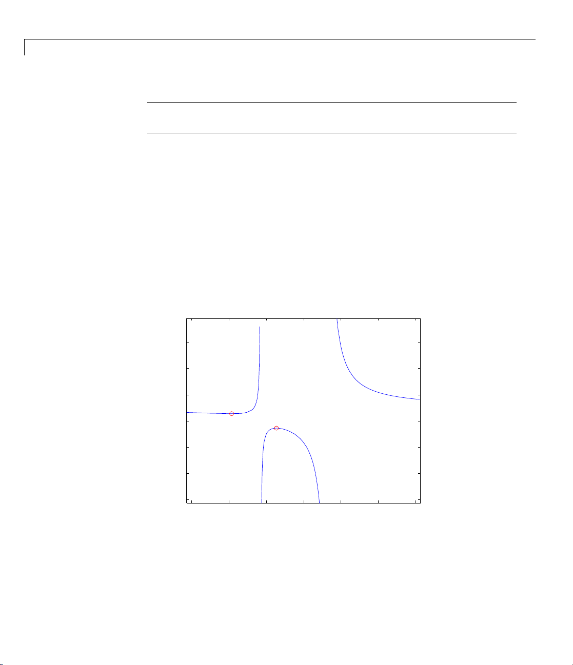
You can plot the maximum and minimum of f with the following commands:
ezplot(f)
hold on
plot(double(crit_pts), double(subs(f,crit_pts)),'ro')
title('Maximum and Minimum of f')
text(-5.5,3.2,'Local minimum')
text(-2.5,2,'Local maximum')
hold off
This displays the following figure.
Maximum and Minimum of f
3-28
8
6
4
Local minimum
2
0
−2
−4
−6 −4 −2 0 2 4 6
Local maximum
x
Finding the Inflection Point
To find the inflection point of f, set the second derivative equal to 0 and solve.
Page 75

f2 = diff(f1);
inflec_pt = solve(f2);
double(inflec_pt)
This returns
ans =
-5.2635
-1.3682 - 0.8511i
-1.3682 + 0.8511i
In this example, only the first entry is a real number, so this is the only
inflection point. (Note that in other examples, the real solutions might not
be the first entries of the answer.) Since you are only interested in the real
solutions, you can discard the last two entries, which are complex numbers.
inflec_pt = inflec_pt(1)
Calculus
To see the symbolic expression for the inflection point, enter
pretty(simplify(inflec_pt))
This returns
/ 1/2 \1/3
13 | 2197 | 8
- -------------------- - | 169/54 - ------- | - -
1\ 18/ 3
/1/2\3
| 169 2197 |
9 | --- - ------- |
\54 18 /
To plot the inflection point, enter
ezplot(f, [-9 6])
hold on
3-29
Page 76

3 Using Symbolic Math Toolbox™ Software
plot(double(inflec_pt), double(subs(f,inflec_pt)),'ro')
title('Inflection Point of f')
text(-7,2,'Inflection point')
hold off
The extra argument, [-9 6],inezplot extends the range of x values in
theplotsothatyouseetheinflectionpoint more clearly, as shown in the
following figure.
8
6
4
Inflection Point of f
2
0
−2
Inflection point
−8 −6 −4 −2 0 2 4 6
x
Extended Calculus Example
This section presents an extended example that illustrates how to find the
maxima and minima of a function. The section covers the following topics:
• “Defining the Function” on page 3-31
• “Finding the Zeros of f3” on page 3-32
• “Finding the Maxima and Minima of f2” on page 3-36
• “Integrating” on page 3-37
3-30
Page 77

Defining the Function
The starting point for the example is the function
Calculus
fxx()
+154
cos( )
.=
You can create the function with the commands
syms x
f = 1/(5+4*cos(x))
which return
f=
1/(4*cos(x) + 5)
The example shows how to find the m aximum and minimum of the second
derivative of f(x). To compute the second derivative, enter
f2 = diff(f, 2)
which returns
f2 =
(4*cos(x))/(4*cos(x) + 5)^2 + (32*sin(x)^2)/(4*cos(x) + 5)^3
Equivalently, you can type f2 = diff(f, x, 2). The default scaling in
ezplot cutsoffpartofthegraphoff2. Youcansettheaxeslimitsmanually
to see the entire function:
ezplot(f2)
axis([-2*pi 2*pi -5 2])
title('Graph of f2')
3-31
Page 78

3 Using Symbolic Math Toolbox™ Software
2
1
0
−1
−2
−3
−4
−5
−6 −4 −2 0 2 4 6
From the graph, it appears that the maximum value of
Graph of f2
x
′′
fx()
is 1 and the
minimum value is -4. As you will see, this is not quite true. To find the exact
values of the maximum and minimum, you only need to find the maximum
and m in
with pe
trans
expla
imum on the interval (–π, π]. This is true because
riod 2π, so that the maxima and minima are simply repeated in each
lation of this interval by an integer multiple of 2π. The next two sections
inhowtodofindthemaximaandminima.
′′
fx()
is periodic
3-32
Finding the Zeros of f3
The maxima and minima of
f3 = diff(f2);
pretty(f3)
compute
′′′
and display it in a more readable form:
fx()
′′
occur at the zeros of
fx()
′′′
.Thestatements
fx()
Page 79

3
384 sin(x) 4 sin(x) 96 cos(x) sin(x)
--------------- - --------------- + ---------------423
(4 cos(x) + 5) (4 cos(x) + 5) (4 cos(x) + 5)
You can simplify this expression using the statements
f3 = simple(f3);
pretty(f3)
2
4 sin(x) (- 16 cos(x) + 80 cos(x) + 71)
----------------------------------------
4
(4 cos(x) + 5)
Calculus
′′′
Now, to find the zeros of
zeros = solve(f3)
fx()
,enter
This returns a 5-by-1 symbolic matrix
zeros =
acos(5/2 - (3*19^(1/2))/4)
acos((3*19^(1/2))/4 + 5/2)
0
-acos(5/2 - (3*19^(1/2))/4)
-acos((3*19^(1/2))/4 + 5/2)
′′′
each of whose entries is a zero of
format;
% Default format of 5 digits
zerosd = double(zeros)
fx()
convert the zeros to double form:
. The commands
3-33
Page 80

3 Using Symbolic Math Toolbox™ Software
zerosd =
2.4483
0 + 2.4381i
0
-2.4483
0 - 2.4381i
So far, you have found three re al zeros and two complex zeros . How ev er, as
the following graph of
ezplot(f3)
hold on;
plot(zerosd,0*zerosd,'ro') % Plot zeros
plot([-2*pi,2*pi], [0,0],'g-.'); % Plot x-axis
title('Graph of f3')
3
f3 shows, these are not all its zeros:
Graph of f3
3-34
2
1
0
−1
−2
−3
−6 −4 −2 0 2 4 6
x
The red circles in the graph correspond to zerosd(1), zerosd(3),and
zerosd(4). As you can see in the graph, there are also zeros at ±π.The
additional zeros occur because
′′′
contains a factor of sin(x), which is
fx()
Page 81

zero at integer multiples of π.Thefunction,solve(sin(x)), however, only
finds the zero at x =0.
′′′
Acompletelistofthezerosof
zerosd = [zerosd(1) zerosd(3) zerosd(4) pi];
fx()
in the interval (–π, π]is
Calculus
Youcandisplaythesezerosonthegraphof
′′′
fx()
commands:
ezplot(f3)
hold on;
plot(zerosd,0*zerosd,'ro')
plot([-2*pi,2*pi], [0,0],'g-.'); % Plot x-axis
title('Zeros of f3')
hold off;
Zeros of f3
3
2
1
0
−1
−2
with the following
−3
−6 −4 −2 0 2 4 6
x
3-35
Page 82

3 Using Symbolic Math Toolbox™ Software
Finding the Maxima and Minima of f2
To find the maxima and minima of
′′′
each of the zeros of
the result below
[zerosd; subs(f2,zerosd)]
ans =
2.4483 0 -2.4483 3.1416
1.0051 0.0494 1.0051 -4.0000
fx()
zeros:
. To do so, substitute zeros into f2 and display
′′
, calculate the value of
fx()
′′
fx()
This shows the following:
′′
fx()
•
•
•
has an absolute maximum at x = ±2.4483, whose value is 1.0051.
′′
fx()
has an absolute minimum at x = π,whosevalueis-4.
′′
has a local minimum at x = 0, whose value is 0.0494.
fx()
You can display the maxima and m inima with the following com mands:
clf
ezplot(f2)
axis([-2*pi 2*pi -4.5 1.5])
ylabel('f2');
title('Maxima and Minima of f2')
hold on
plot(zerosd, subs(f2,zerosd), 'ro')
text(-4, 1.25, 'Absolute maximum')
text(-1,-0.25,'Local minimum')
text(.9, 1.25, 'Absolute maximum')
text(1.6, -4.25, 'Absolute minimum')
hold off;
at
3-36
This displays the following figure.
Page 83

Calculus
Maxima and Minima of f2
1
Absolute maximum
Absolute maximum
0
−1
f2
−2
−3
−4
−6 −4 −2 0 2 4 6
Local minimum
Absolute minimum
x
The preceding analysis shows that the actual range of
Integrating
Integrate f(x):
F = int(f)
The result
′′
is [–4, 1.0051].
fx()
F=
(2*atan(tan(x/2)/3))/3
involves the arctangent function.
Note that F(x) is not an antiderivative of f(x) for all real numbers, since it is
discontinuous at odd multiples of π,wheretan (x)issingular.Youcanseethe
gaps in F(x) in the following figure.
ezplot(F)
3-37
Page 84

3 Using Symbolic Math Toolbox™ Software
3-38
To change F(x) into a true antiderivative of f(x) that is differentiable
everywhere, you can add a step function to F(x). The height of the steps is
the h eight of the gaps in the graph of F(x). You can determine the height of
the gaps by taking the limits of F(x)asx approaches π from the left and from
the right. The limit from the left is
limit(F, x, pi, 'left')
ans =
pi/3
On the other hand, the limit from the right is
limit(F, x, pi, 'right')
ans =
-pi/3
The height of the gap is the distance between the left-and right-hand limits,
which is 2π/3 as shown in the following figure.
Page 85

You can create the step function using the round function, which rounds
numbers to the nearest integer, as follows:
Calculus
J = sym(2*
pi/3)*sym('round(x/(2*pi))');
Each step has width 2π, and the jump from one step to the next is 2π/3, as
shown in the following figure, generated with
ezplot
(J, [-2*pi 2*pi])
3-39
Page 86

3 Using Symbolic Math Toolbox™ Software
3-40
Next, add the step function J(x)toF(x) with the following code:
F1=F+J
F1 =
(2*atan(tan(x/2)/3))/3 + (2*pi*round(x/(2*pi)))/3
Adding the step function raises the section of the graph of F(x)ontheinterval
[π,3π)upby2π/3, lowers the section on the interval (–3π,–π]downby2π/3,
and so on, as show n in the following figure.
Page 87

Calculus
When you plo
ezplot(F1)
t the result by entering
you s ee that this representation does have a continuous graph.
3-41
Page 88

3 Using Symbolic Math Toolbox™ Software
Simplifications and Substitutions
In this section...
“Simplifications” on page 3-42
“Substitutions” on page 3-53
Simplifications
Here are three different symbolic expressions.
syms x
f = x^3 - 6*x^2 + 11*x - 6;
g = (x - 1)*(x - 2)*(x - 3);
h = -6 + (11 + (-6 + x)*x)*x;
Here are their prettyprinted forms, generated by
3-42
pretty(f);
pretty(g);
pretty(h)
32
x -6x +11x-6
(x-1)(x-2)(x-3)
x(x(x-6)+11)-6
These expressions are three different representations of the same
mathematical function, a cubic polynomial in
Each of the three forms is preferable to the others in different situations. The
first form,
is simply a linear combination of the powers of
factored form. It displays the roots of the polynomial and is the most accurate
for numerical evaluation near the roots. But, if a polynomial does not have
such simple roots, its factored form may notbesoconvenient. Thethirdform,
f, is the most commonly used representation of a polynomial. It
x.
x. The second form, g,isthe
Page 89

Simplifications and Substitutions
h, is the Horner, or nested, representation. For numerical evaluation, it
involves the fewest arithmetic operations and is the most accurate for some
other ranges of
x.
The symbolic simplification problem involves the verification that these three
expressions represent the same function. It also involves a less clearly defined
objective — which of these representations is “the simplest”?
This toolbox provides seve r al functions that apply various algebraic and
trigonometric identities to transform one representation of a function into
another, possibly simpler, representation. These functions are
expand, horner, factor, simplify,andsimple.
collect,
collect
The statementcollect(f) views f as a polynomial in its symbolic variable,
say
x, and collects all the coefficients with the same power of x.Asecond
argument can specify the variable in which to collect terms if there is more
than one candidate. Here are a few examples.
f collect(f)
syms x;
f=
(x-1)*(x-2)*(x-3);
syms x;
f = x*(x*(x - 6) +
11) - 6;
syms x t;
f = (1+x)*t + x*t;
collect(f)
ans =
x^3 - 6*x^2 + 11*x - 6
collect(f)
ans =
x^3 - 6*x^2 + 11*x - 6
collect(f)
ans =
(2*t)*x + t
3-43
Page 90

3 Using Symbolic Math Toolbox™ Software
expand
The statement expand(f) distributes products over sums and applies other
identities involving functions of sumsasshownintheexamplesbelow.
fexpand(f)
syms a x y;
f = a*(x + y);
syms x;
f = (x - 1)*(x
- 2)*(x - 3);
syms x;
f = x*(x*(x -
6) + 11) - 6;
syms a b;
f = exp(a + b);
syms x y;
f = cos(x + y);
expand(f)
ans =
a*x + a*y
expand(f)
ans =
x^3 - 6*x^2 + 11*x - 6
expand(f)
ans =
x^3 - 6*x^2 + 11*x - 6
expand(f)
ans =
exp(a)*exp(b)
expand(f)
ans =
cos(x)*cos(y) - sin(x)*sin(y)
3-44
Page 91

fexpand(f)
Simplifications and Substitutions
syms x;
f=
cos(3*acos(x));
syms x;
f = 3*x*(x^2 -
1) + x^3;
expand(f)
ans =
3*x*(x^2 - 1) + x^3
expand(f)
ans =
4*x^3 - 3*x
horner
The statement horner(f) transforms a symbolic polynomial f in to its Horner,
or nested, representation as shown in the following examples.
fhorner(f)
syms x;
f = x^3 - 6*x^2
+ 11*x - 6;
syms x;
f = 1.1 + 2.2*x
+ 3.3*x^2;
horner(f)
ans =
x*(x*(x - 6) + 11) - 6
horner(f)
ans =
x*((33*x)/10 + 11/5) + 11/10
factor
If f is a polynomial with rational coefficients, the statement
factor(f)
expresses f as a product of polynomials of lower degree with rational
coefficients. If
f itself. Here are several exam ples.
f cannot be factored over the rational numbers, the result is
3-45
Page 92

3 Using Symbolic Math Toolbox™ Software
ffactor(f)
syms x;
f = x^3 - 6*x^2
+ 11*x - 6;
syms x;
f = x^3 - 6*x^2
+ 11*x - 5;
syms x;
f=x^6+1;
factor(f)
ans =
(x - 3)*(x - 1)*(x - 2)
factor(f)
ans =
x^3 - 6*x^2 + 11*x - 5
factor(f)
ans =
(x^2 + 1)*(x^4 - x^2 + 1)
Here is another example involving factor. It factors polynomials of the form
x^n + 1.Thiscode
syms x;
n = (1:9)';
p = x.^n + 1;
f = factor(p);
[p, f]
3-46
returns a matrix with the polynomials in its first column and their factored
forms in its second.
ans =
[ x+1, x+1]
[ x^2 + 1, x^2 + 1]
[ x^3 + 1, (x + 1)*(x^2 - x + 1)]
[ x^4 + 1, x^4 + 1]
[ x^5 + 1, (x + 1)*(x^4 - x^3 + x^2 - x + 1)]
[ x^6 + 1, (x^2 + 1)*(x^4 - x^2 + 1)]
[ x^7 + 1, (x + 1)*(x^6 - x^5 + x^4 - x^3 + x^2 - x + 1)]
[ x^8 + 1, x^8 + 1]
[ x^9 + 1, (x + 1)*(x^2 - x + 1)*(x^6 - x^3 + 1)]
Page 93

Simplifications and Substitutions
As an aside at this point, factor can also factor symbolic objects containing
integers. This is an alternative to using the
specfun directory. For example, the fo ll owing code segment
N = sym(1);
for k = 2:11
N(k) = 10*N(k-1)+1;
end
[N' factor(N')]
factor function in the MATLAB
displays the factors of symbolic integers consisting of 1s:
ans =
[1, 1]
[ 11, 11]
[ 111, 3*37]
[ 1111, 11*101]
[ 11111, 41*271]
[ 111111, 3*7*11*13*37]
[ 1111111, 239*4649]
[ 11111111, 11*73*101*137]
[ 111111111, 3^2*37*333667]
[ 1111111111, 11*41*271*9091]
[ 11111111111, 21649*513239]
simplify
The simplify function is a powerful, general purpose tool that applies a
number of algebraic identities involving sums, integral powers, square roots
and other fractional powers, as well as a number of functional identities
involving trig functions, exponential and log functions, Bessel functions,
hypergeometric functions, and the gamma function. Here are some examples.
3-47
Page 94

3 Using Symbolic Math Toolbox™ Software
f simplify(f)
syms x;
f = x*(x*(x - 6) +
11) - 6;
syms x;
f = (1 - x^2)/(1 - x);
syms a;
f = (1/a^3 + 6/a^2 +
12/a + 8)^(1/3);
syms x y;
f = exp(x) * exp(y);
syms x;
f = besselj(2, x) +
besselj(0, x);
simplify(f)
ans =
(x - 1)*(x - 2)*(x - 3)
simplify(f)
ans =
x+1
simplify(f)
ans =
((2*a + 1)^3/a^3)^(1/3)
simplify(f)
ans =
exp(x + y)
simplify(f)
ans =
(2*besselj(1, x))/x
3-48
syms x;
f = gamma(x + 1) x*gamma(x);
syms x;
f = cos(x)^2 + sin(x)^2;
simplify(f)
ans =
0
simplify(f)
ans =
1
Page 95

Simplifications and Substitutions
You can also use the syntax simplify(f, n) where n is a positive integer
that controls how many steps
provide an argument
syms x;
z = 3 - 1/sin(x)^2 - cot(x)^2
z=
3 - 1/sin(x)^2 - cot(x)^2
simplify(z)
ans =
4 - 2/sin(x)^2
simplify(z, 200)
ans =
2 - 2*cot(x)^2
n, is 100 steps. For example,
simplify takes. The default, when you don’t
simple
The simple function has the unorthodox mathematical goal of finding a
simplification of an expression that has the fewest number of characters.
Of course, there is little mathematical justi fication for claiming that one
expression is “simpler” than another just because its ASCII representation is
shorter, but this often proves satisfactory in practice.
The
simple function achieves its goal by independently applying simplify,
collect, factor, and o th er simplification functions to an expression and
keeping track of the lengths of the results. The
the shortest result.
The
simple function has several forms, each returning different output. The
form
simple(f) displays each trial sim plification and the simplification
function that produced it in the MATLAB command window. The
function then returns the shortest result. For example, the command
syms x;
simple(cos(x)^2 + sin(x)^2)
simple function then returns
simple
3-49
Page 96

3 Using Symbolic Math Toolbox™ Software
displays the following alternative simplifications in the MATLAB command
window along with the result:
simplify:
1
radsimp:
cos(x)^2 + sin(x)^2
simplify(100):
1
combine(sincos):
1
combine(sinhcosh):
cos(x)^2 + sin(x)^2
combine(ln):
cos(x)^2 + sin(x)^2
3-50
factor:
cos(x)^2 + sin(x)^2
expand:
cos(x)^2 + sin(x)^2
combine:
cos(x)^2 + sin(x)^2
rewrite(exp):
((1/exp(x*i))/2 + exp(x*i)/2)^2 + (((1/exp(x*i))*i)/2 - (exp(x*i)*i)/2)^2
rewrite(sincos):
cos(x)^2 + sin(x)^2
rewrite(sinhcosh):
cosh(-x*i)^2 - sinh(-i*x)^2
rewrite(tan):
Page 97

Simplifications and Substitutions
(tan(x/2)^2 - 1)^2/(tan(x/2)^2 + 1)^2 + (4*tan(x/2)^2)/(tan(x/2)^2 + 1)^2
mwcos2sin:
1
collect(x):
cos(x)^2 + sin(x)^2
ans =
1
This form is useful when you want to check, for example, whether the shortest
form is indeed the simplest. If you are not interested in how
its result, use the form
f = simple(f). This form simply returns the shortest
simple achieves
expression found. For example, the statement
f = simple(cos(x)^2 + sin(x)^2)
returns
f=
1
If you want to know which simplification returned the shortest result, use the
multiple output form
[f, how] = simple(f). This form returns the shortest
result in the first variable and th e simplification method used to achieve the
result in the second variable. For example, the statement
[f, how] = simple(cos(x)^2 + sin(x)^2)
returns
f=
1
how =
simplify
The simple function sometimes improves on the result returned by simplify,
one of the simplifications that it tries. Fo r example, when applied to the
3-51
Page 98

3 Using Symbolic Math Toolbox™ Software
examples given for simplify, simple returns a simpler (or at least shorter)
result as shown:
f simplify(f) simple(f)
syms a positive;
f = (1/a^3 + 6/a^2 +
12/a + 8)^(1/3);
syms x;
f = cos(x) + i*sin(x);
simplify(f)
ans =
(8*a^3 + 12*a^2 +
6*a + 1)^(1/3)/a
simplify(f)
ans =
cos(x) + sin(x)*i
g=
simple(f)
g=
1/a + 2
g=
simple(f)
g=
exp(x*i)
In some cases, it is advantageous to apply simple twicetoobtaintheeffectof
two different s implification functions. For example:
syms x;
z = exp((cos(x)^2 - sin(x)^2)/(sin(x)*cos(x)))
z=
exp((cos(x)^2 - sin(x)^2)/(cos(x)*sin(x)))
z1 = simple(z)
3-52
z1 =
exp(cot(x) - tan(x))
z2 = simple(simple(z))
z2 =
exp(2/tan(2*x))
The simple function is particularly effective on expressions involving
trigonometric functions:
Page 99

Simplifications and Substitutions
fsimple(f)
syms x;
f = cos(x)^2 +
sin(x)^2;
syms x;
f = 2*cos(x)^2 sin(x)^2;
syms x;
f = cos(x)^2 sin(x)^2;
syms x;
f = cos(x) +
i*sin(x);
syms x;
f = cos(3*acos(x));
f = simple(f)
f=
1
f = simple(f)
f=
2 - 3*sin(x)^2
f = simple(f)
f=
cos(2*x)
f = simple(f)
f=
exp(x*i)
f = simple(f)
f=
4*x^3 - 3*x
Substitutions
There are two functions for symbolic substitution: subexpr and subs.
subexpr
These commands
syms a x
s = solve(x^3 + a*x + 1)
3-53
Page 100

3 Using Symbolic Math Toolbox™ Software
solve the equation x^3+a*x+1=0for the variable x:
s=
((a^3/27 + 1/4)^(1/2) - 1/2)^(1/3) - a/(3*((a^3/27 + 1/4)^(1/2) - 1/2)^(1/3))
a/(6*((a^3/27 + 1/4)^(1/2) - 1/2)^(1/3)) - ((a^3/27 + 1/4)^(1/2) - 1/2)^(1/3)/2...
- (3^(1/2)*(a/(3*((a^3/27 + 1/4)^(1/2) - 1/2)^(1/3))...
+ ((a^3/27 + 1/4)^(1/2) - 1/2)^(1/3))*i)/2
a/(6*((a^3/27 + 1/4)^(1/2) - 1/2)^(1/3)) - ((a^3/27 + 1/4)^(1/2) - 1/2)^(1/3)/2...
+ (3^(1/2)*(a/(3*((a^3/27 + 1/4)^(1/2) - 1/2)^(1/3))...
+ ((a^3/27 + 1/4)^(1/2) - 1/2)^(1/3))*i)/2
This long expression has many repeated pieces, or subexpressions. The
subexpr function allows you to save these common subexpressions as
well as the symbolic object rewritten in terms of the subexpressions. The
subexpressions a re saved in a column vector called
Continuing with the example
sigma.
3-54
r = subexpr(s)
returns
sigma =
(a^3/27 + 1/4)^(1/2) - 1/2
r=
sigma^(1/3) - a/(3*sigma^(1/3))
a/(6*sigma^(1/3)) - sigma^(1/3)/2 - (3^(1/2)*(a/(3*sigma^(1/3)) + sigma^(1/3))*i)/2
a/(6*sigma^(1/3)) - sigma^(1/3)/2 + (3^(1/2)*(a/(3*sigma^(1/3)) + sigma^(1/3))*i)/2
Notice that subexpr creates the variable sigma in the MATLAB w orkspace.
You can verify this by typing
sigma
whos, or the command
which returns
sigma =
(a^3/27 + 1/4)^(1/2) - 1/2
 Loading...