Mathworks SPLINE TOOLBOX 3 user guide

Spline Toolbox™ 3

User’s Guide

How to Contact The MathWorks

www.mathworks.
comp.soft-sys.matlab Newsgroup
www.mathworks.com/contact_TS.html T echnical Support

[e-mail] Product enhancement suggestions

bugs@mathwo
[e-mail] Documentation error reports
[e-mail] Order status, license renewals, passcodes

info@mathwo

com

rks.com

rks.com

Web

Bug reports

Sales, prici

ng, and general information

508-647-7000 (Phone)

508-647-7001 (Fax)

The MathWorks, Inc.
3 Apple Hill Drive
Natick, MA 01760-2098

For contact information about worldwide offices, see the MathWorks Web site.

Spline Toolbox™ User’s Guide

© COPYRIGHT 1990–20 10 by The MathWorks, Inc.

The software described in this document is furnished under a license agreement. The software may be used
or copied only under the terms of the license agreement. No part of this manual may be photocopied or
reproduced in any form without prior written consent from The MathW orks, Inc.

FEDERAL ACQUISITION: This provision applies to all acquisitions of the Program and Documentation
by, for, or through the federal government of the United States. By accepting delivery of the Program
or Documentation, the government hereby agrees that this software or documentation qualifies as
commercial computer software or commercial computer software documentation as such terms are used
or defined in FAR 12.212, DFARS Part 227.72, and DFARS 252.227-7014. Accordingly, the terms and
conditions of this Agreement and only those rights specified in this Agreement, shall pertain to and govern
theuse,modification,reproduction,release,performance,display,anddisclosureoftheProgramand
Documentation by the federal government (or other entity acquiring for or through the federal government)
and shall supersede any conflicting contractual terms or conditions. If this License fails to meet the
government’s needs or is inconsistent in any respect with federal procurement law, the government agrees
to return the Program and Docu mentation, unused, to The MathWorks, Inc.

Trademarks

MATLAB and Simulink are registered trademarks of The MathWorks, Inc. See

www.mathworks.com/trademarks for a list of additional trademarks. Other product or brand

names may be trademarks or registered trademarks of their respective holders.

Patents

The MathWorks products are protected by one or more U.S. patents. Please see

www.mathworks.com/patents for more information.

Revision History

March 1990 First printing New for Version 1.0
November 1992 Second printing Revised for Version 1.1
January 1998 Third printing Revised for Version 2.0 (Release 10)
January 1999 Online only Revised for Version 2.0.1 (Release 11)
September 2000 Fourth printing Revised for Version 3.0 (Release 12)
May 2001 Fifth printing Minor revision for Version 3.0 (Release 12.1)
December 2001 Online only Revised for Version 3.1
February 2003 Sixth printing Revised for Version 3.2 (Release 13)
June 2004 Seventh printing Revised for Version 3.2.1 (Release 14)
June 2005 Eighth printing Minor revision for Version 3.2.1
September 2005 Online only Minor revision for Version 3.2.2 (Release 14SP3)
March 2006 Ninth printing Revised for Version 3.3 (Release 2006a)
September 2006 Online only Minor revision for Version 3.3.1 (Release 2006b)
September 2006 Tenth printing Version 3.3.1
March 2007 Online only Revised for Version 3.3.2 (Release 2007a)
May 2007 Eleventh printing Version 3.3.2
September 2007 Online only Revised for Version 3.3.3 (Release 2007b)
March 2008 Online only Revised for Version 3.3.4 (Release 2008a)
October 2008 Online only Revised for Version 3.3.5 (Release 2008b)
March 2009 Online only Revised for Version 3.3.6 (Release 2009a)
September 2009 Online only Revised for Version 3.3.7 (Release 2009b)
March 2010 Online only Revised for Version 3.3.8 (Release 2010a)

Acknowledgments

The MathWorks™ would like to acknowledge the contributions of Carl de
Boor to the Spline Toolbox™. Professor de Boor authored the Spline Toolbox

from its first release until Version 3.3.4 (2008).

Professor de Boor received the John von Neumann Prize in 1996 and the
National Medal of Science in 2003. He is a member of both the American
Academy of Arts and Sciences and the National Academy of Sciences. He is
the a uthor of A Practical Guide to Splines (Springer, 2001).

Acknowledgments

Acknowledgments

Getting Started

1

Product Overview ................................. 1-2

Contents

MATLAB Splines

Expected Background

Technical Conventions

Vectors
Naming Conventions
Using Spline Toolbox Functions

.......................................... 1-6

.................................. 1-4

.............................. 1-5

............................. 1-6

............................... 1-6

...................... 1-7

Some Simple Examples

2

Introduction ...................................... 2-2

Cubic Spline Interpolation

Cubic Spline Interpolant of Smooth Data
Periodic Data
Other End Conditions
General Spline Interpolation
Knot Choices
Smoothing
Least Squares

..................................... 2-4

..................................... 2-7

....................................... 2-8

.................................... 2-10

......................... 2-3

.............. 2-3

.............................. 2-5

........................ 2-5

Using the Spline Fits

Vector-Valued Functions

............................... 2-11

........................... 2-12

vii

Fitting Values at N-D Grid .......................... 2-15

Fitting Values at Scattered 2-D Sites

................ 2-18

Splines: An Overview

3

Introduction ...................................... 3-2

Polynomials vs. Splines

ppform

B-form

Knot Multiplicity

B-Spline Properties

Constructive vs. Variational

........................................... 3-4

............................................ 3-5

.................................. 3-6

............................ 3-3

................................ 3-7

........................ 3-8

viii Contents

Multivariate Splines

Rational Splines

............................... 3-10

................................... 3-12

The ppform

4

Introduction ...................................... 4-2

ppform

........................................... 4-3

Construction ...................................... 4-4

Available Commands

............................... 4-6

The B-form

5

Introduction ...................................... 5-2

B-form

B-Splines

Knot Multiplicity

Choice of Knots

Splines

Construction

............................................ 5-3

......................................... 5-4

.................................. 5-5

.................................... 5-7

........................................... 5-8

...................................... 5-9

Example: A Spline Curve

Available Commands

........................... 5-10

............................... 5-12

Tensor Product Splines

6

Introduction ...................................... 6-2

B-form

............................................ 6-3

ix

Construction and Use .............................. 6-4

ppform

Example: The Mobius Band

........................................... 6-5

......................... 6-6

NURBS and Other Rational Splines

7

Introduction ...................................... 7-2

Example: Circle

Example: Sphere

rsform: rpform, rBform

Available Commands

................................... 7-3

.................................. 7-5

............................ 7-6

............................... 7-8

x Contents

The stform

8

Introduction ...................................... 8-2

Properties of the stform

Available Commands

............................ 8-3

............................... 8-5

Advanced Examples

9

Least-Squares Approximation by “Natural” Cubic

Splines

Problem
General Resolution
Need for a Basis Map
A Basis Map for “Natural” Cubic Splines
TheOne-lineSolution
The Nee d for Proper Extrapolation
The Correct One-Line Solution
Least-Squares Approximation by Cubic Splines

......................................... 9-2

......................................... 9-2

................................ 9-2

.............................. 9-3

.............................. 9-4

................... 9-4

....................... 9-6

.............. 9-3

......... 9-7

A Nonlinear ODE

Problem
Approximation Space
Discretization
Numerical Problem
Linearization
Linear System to Be Solved
Iteration

Construction of the Chebyshev Spline

What Is a Chebyshev Spline?
Choice of Spline Space
Initial Guess
Remez Iteration

Approximation by Tensor Product Splines

Choice of Sites and Knots
Least Squares Approximation as Function of y
ApproximationtoCoefficientsasFunctionsofx
The Bivariate Approximation
Switch in Order
ApproximationtoCoefficientsasFunctionsofy
The Bivariate Approximation
Comparison and Extension

......................................... 9-8

......................................... 9-11

.................................. 9-8

.............................. 9-8

.................................... 9-9

................................ 9-9

..................................... 9-10

......................... 9-10

............... 9-14

........................ 9-14

............................. 9-14

..................................... 9-15

................................... 9-16

........................... 9-20

........................ 9-23

................................... 9-25

........................ 9-27

.......................... 9-28

........... 9-20

.......... 9-21

......... 9-22

......... 9-26

xi

10

Function Reference

GUIs .............................................. 10-2

11

Construction of Splines

Operators

Work with Breaks, Knots, and Sites

Customized Linear Equation Solver

Information About Splines and the Toolbox

Utilities

......................................... 10-4

........................................... 10-8

............................ 10-3

................. 10-5

................. 10-6

Functions – Alphabetical List

.......... 10-7

Glossary

xii Contents

A

Introduction ...................................... A-2

List of Terms

...................................... A-3

Getting Started

• “Product Overview” on page 1-2

• “MATLAB Splines” on page 1-4

• “Expected Background” on p age 1-5

• “Technical Conventions” on page 1-6

1

1 Getting Started

Product Overview

Spline Toolbox software contains versions of the essential MATLAB
programsoftheB-splinepackage(extendedtohandlealsovector-valued
splines) as described in A Practical Guide t o Splines, (Applied Math. Sciences
Vol. 27, Springer Verlag, New York (1978), xxiv + 392p; revised edition
(2001),xviii+346p),hereafter referred to a s PGS. The toolbox makes it easy to
create and work with piecewise-polynomial functions.

The typical use envisioned for this toolbox involves the construction and
subsequent use of a piecewise-polynomial approximation. This construction
would involve data fitting, but there is a wide range of possible data that
could be fit. In the simplest situation, one is given points (ti,yi) and is looking
for a piecewise-polynomial function f that satisfies f(ti)=yi, all i, more or less.
An exact fit would involve interpolation, an approximate fit might involve
least-squares approximation or the smoothing spline. But the function to be
approximated may also be described in more implicit ways, for example as the
solution of a differential or integral equation. In such a case, the data would
be of the form (Af)(ti), with A some differential or integral operator. On the
other hand, one might want to construct a spline curve whose exact location is
less important than is its overall shape. Finally, in all of this, one might be
looking for functions of more than one variable, such as tensor product splines.

Carehasbeentakentomakethisworkaspainlessandintuitiveaspossible.
In particular, the user need not worry about just how splines are constructed
or stored for later use, nor need the casual user worry about such items as
“breaks” or “knots” or “coefficients”. It is enough to know that each function
constructed is just another variable that is freely usable as input (where
appropriate) to many of the commands, including all commands beginning
with

fn, which stands for function.Attimes,itmaybealsousefultoknow

that, internal to the toolbo x, splines are stored in different forms, with the
command

fn2fm available to convert between forms.

®

1-2

At present, the toolbox supports two major forms for the representation of
piecewise-polynomial functions, because each has been found to be superior
to the other in certain common situations. The B-form is particularly useful
during the construction of a spline, while the ppform is more efficient when
the piecewise-polynomial function is to be evaluated extensiv ely . T he se two
forms are almost exactly the B-representation and the pp representation
used in PGS.

Product Overview

But, over the years, the Spline Toolbox product has gone beyond the programs
in PGS. The toolbox now supports the ‘scattered translates’ form, or stform,
in order to handle the construction and use of bivariate thin-plate splines,
and also two ways to represent rational splines, the rBform and the rpform,
inordertohandleNURBS.

Splines can be very effective for data fitting because the linear systems to be
solved for this are banded, hence the work needed for their solution, done
properly, grows only linearly with the number of data points. In particular,
the M ATL AB sparse m atrix facilities are used in the Spline Toolbox product
when that is more efficient than the toolbox’s own equation solver,

slvblk,

which relies on the fact that some of the linear systems here are even almost
block diagonal.

All polynomial spline construction commands are equipped to produce
bivariate (or even mu lti variate) piecewise-polynomial functions as tensor
products of the univariate functions used here, and the various

fn...

commands also work for these multivariate functions.

There are various examples, all accessible through the Demos tab in the
MATLAB Help b row se r. You are strongly urged to have a look at some of
them, or at the GUI

splinetool, before attempting to use this toolbox, or

even before reading on.

1-3

1 Getting Started

MATLAB Splines

The MATLAB technical computing environment provides spline
approximation via the command

spline(x,y)
x that takes the value y(i) at x(i),alli, and satisfies the not-a-knot end

condition. In other words, the command
result as the command
product. But only the latter also works when
data. In MATLAB, cubic spline interpolation to multivar iate g r idded data is
provided by the command
which returns values of the interpolating tensor product cubic spline at the
grid specified by

, it returns the ppform of the cubic spline with break sequence

cs = csapi(x,y) available in the Spline Toolbox

interpn(x1,...,xd,v,y1,...,yd,'spline')

y1,...,yd.

spline.Ifcalledintheformcs =

cs = spline(x,y) gives the same

x,y describe multivariate gridded

Further, any of the Spline Toolbox
output of the MATLAB
the Spline Toolbox commands
MATLAB, as the commands

spline(x,y) command, with simple versions of

fnval, ppmak, fnbrk available directly in

ppval, mkpp, unmkpp, respectively.

fn... commands can be applied to the

1-4

Expected Background

The Spline Toolbox product started out as an extension of the MATLAB
environment of interest to experts in spline approximation, to aid them in the
construction and testing of new methods of spline approximation. Such people
will have maste red the material in PGS.

However, the basic toolbox commands, for constructing and using spline
approximations,aresetuptobeusablewithnomoreknowledgethanit
takes to understand what it means to, say, construct an interpolant or a
least squares approximant to some data, or what it means to differentiate or
integrate a function.

With that in mind, there are sections, like Chapter 2, “Some Simple
Examples”, that are meant even for the novice, while sections devoted to
a detailed example, like the one on constructing a Chebyshev spline or on
constructing and using tensor products, are meant for users interested in
developing their own spline commands.

Expected Background

A “Glossary” at the end of this guide provides definitions of almost all the
mathematical terms used in this document.

1-5

1 Getting Started

Technical Conventions

• “Vectors” on page 1-6

• “Naming Conventions” on page 1-6

• “Using Spline Toolbox Functions” on page 1-7

Vectors

The Spline Toolbox product can handle vector-valued splines, i.e., splines
whose values lie in R
type, that of a matrix, there is even now some uncertainty about how to deal
with vectors, i.e., lists of numbers. MATLAB sometimes stores s uch a list in a
matrix with just one row, and other times in a matrix with just one column.
In the first instance, such a 1-row matrix is called a row-vector; in the second
instance, such a 1-column matrix is called a column-vector. Either way, these
are merely different ways for storing vectors, not different kinds of vectors.

In this toolbox, vectors,i.e.,listsofnumbers,mayalsoendupstoredina
1-row matrix or in a 1-column matrix, but with the following agreements.

d

. Since MATLAB started out with just one variable

1-6

ApointinR
particular, if you want to supply an
you are expected to provide that list as the

While other lists of numbers (e.g., a knot sequence or a break sequence) may
be stored internally as row vectors, youmaysupplysuchlistsasyouplease,
as a row vector or a column vector.

d

, i.e., a d-vector, is always stored as a column vector. In

n-list of d-vectors to one of the commands,

n columns of a matrix of size [d,n].

Naming Conventions

MostoftheSplineToolboxcommandsin this toolbox have names that follow
one of the f ollowing patterns:

cs... commands construct cubic splines (in ppform)

sp... commands construct splines in B-form

fn... commands operate on spline functions

Technical Conventions

..2.. comm ands convert something

..api commands construct an approximation by interpolatio n

..aps commands construct an approximation by smoothing

..ap2 commands construct a least-squares approximation

...knt commands construct (part of) a particular knot sequence

...dem commands are demonstrations now reached via the Demos tag in

the MATLAB Help browser.

Some of these naming conventions are the result of a discussion with Jörg
Peters, then a graduate student in Computer Sciences at the University of
Wisconsin-Madison.

Note See the “Glossary” for information about notation used in this book.

Using Spline Toolbox Functions

For ease of use, most Spline Toolbox functions have default argu ments. In
the reference entry under Syntax, we usually first list the function with all
necessary input arguments and then with all possible input arguments. When
there is more than one optional argument, then, sometimes, but not always,
their exact order is immaterial. When their order does matter, you have to
specify every optional argument preceding the one(s) you are interested in.
In this situation, you can specify the default value for an optional argument
by using
reference page tells you the default value for each optional input argument.

As in MATLAB, only the output arguments e xp lic itly specified are returned
to the user.

[] (the empty matrix) as the input for it. The description in the

1-7

1 Getting Started

1-8

Some Simple Examples

• “Introduction” on page 2-2

• “Cubic Spline Interpolation” on page 2-3

• “Using the Spline Fits” on page 2-11

• “Vector-Valued Functions” on page 2-12

• “Fitting Values at N-D Grid” on page 2-15

• “Fitting Values at Scattered 2 -D Sites” on page 2-18

2

2 Some Simple Examples

Introduction

These examples provide some simple ways to make use of the commands in
this toolbox. More complicated examples are given in later sections. Other
examples are available in the various demos, all of which can be reached by
the Demos tab in the MATLAB Help browser. In addition, the command

splinetool provides a g raphical user interface (GUI) for you to try several of

the basic sp li n e interpolation and approximatio n commands from this toolbox
on your data; it even provides various instructive data sets.

Check the reference pages if you have specific questions about the use of the
commands mentioned. Check the Glossary if you hav e specific questions
about the terminology used; a look into the Index may help.

2-2

Cubic Spline Interpolation

In this section...

“Cubic Spline Interpolant of Smooth Data” on page 2-3

“Periodic Data” on page 2-4

“Other End Conditions” on page 2-5

“General Spline Interp olation” on page 2-5

“Knot Choices” o n page 2-7

“Smoothing” on page 2-8

“Least Squares” on page 2-10

Cubic Spline Interpolant of Smooth Data

Suppose you want to interpolate some smooth data, e.g., to

rand('seed',6), x = (4*pi)*[0 1 rand(1,15)]; y = sin(x);

Cubic Spline Interpolation

You can use the cubic spline interpolant obtained by

cs = csapi(x,y);

and plot the spline, along with the data, with the following code:

fnplt(cs);
hold on
plot(x,y,'o')
legend('cubic spline','data')
hold off

This produces a figure like the followin g.

2-3

2 Some Simple Examples

2-4

Cubic Spline Interpolant of Smooth Data

This is, more precisely, the cubic spline interpolant with the not-a-knot end
conditions, meaning that it is the unique piecewise cubic polynomial with two
continuous derivatives with breaks at all interior data sites except for the
leftmost and the rightmost one. It is the same interpolant as produced by the
MATLAB

spline command, spline(x,y).

Periodic Data

Thesinefunctionis2π-periodic. To check how well your interpolant does on
that score, compute, e.g., the difference in the value of its first derivative
at the two endpoints,

diff(fnval(fnder(cs),[0 4*pi]))

Cubic Spline Interpolation

ans = -.0100

which is not so good. If you prefer to get an interpolant whose first and second
derivatives at the two endpoints,

csape which permits specification of many different kinds of end conditions,

0 and 4*pi,match,useinsteadthecommand

including periodic end conditions. So, use instead

pcs = csape(x,y,'periodic');

for which you get

diff(fnval(fnder(pcs),[0 4*pi]))

Output is ans=0as the difference of end slopes. Even the difference in end
second derivatives is small:

diff(fnval(fnder(pcs,2),[0 4*pi]))

Output is ans = -4.6074e-015.

Other End Conditions

Other end conditions can be handled as well. For example,

cs = csape(x,[3,y,-4],[1 2]);

provides the cubic spline interpolant with breaks at the and with its slope
at the leftmost data site equal to 3, and its second derivative at the rightmost
data site equal to -4.

General Spline Interpolation

If you want to interpolate at sites other than the breaks and/or by splines
other than cubic splines with simple knots, then you use the
In its simplest form, y ou would say
argument,

k,specifiestheorder of the interpolating spline; this is the number

sp = spapi(k,x,y);inwhichthefirst

of coefficients in each polynomial piece, i.e., 1 mo re than the nominal degree of
its polynomial pieces. For example, the next figure shows a linear, a quadratic,
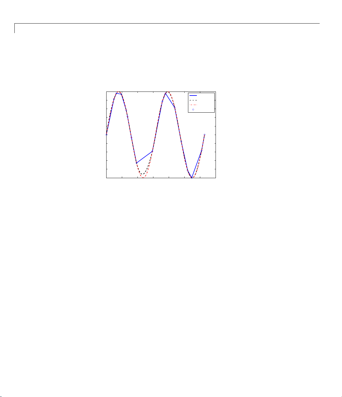
and a quartic spline interpolant to your data, as obtained by the statements

sp2 = spapi(2,x,y); fnplt(sp2,2), hold on

spapi command.

2-5

2 Some Simple Examples

sp3 = spapi(3,x,y); fnplt(sp3,2,'k--'), set(gca,'Fontsize',16)
sp5 = spapi(5,x,y); fnplt(sp5,2,'r-.'), plot(x,y,'o')
legend('linear','quadratic','quartic','data'), hold off

1

0.8

0.6

0.4

0.2
0

−0.2

−0.4

−0.6

−0.8

−1
0 2 4 6 8 10 12 14

linear
quadratic
quartic
data

Spline Interpolants of Various Orders of Smooth Data

Even the cubic spline interpolant obtained from spapi is different from the
one provided by

csapi and spline. To emphasize their difference, compute

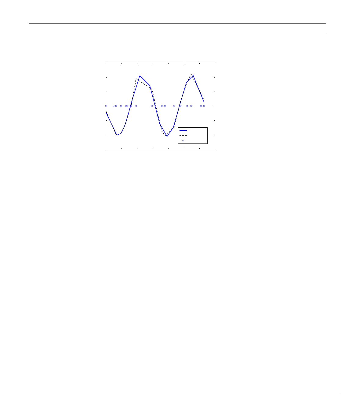
and plot their second derivatives, as follows:

fnplt(fnder(spapi(4,x,y),2)), hold on, set(gca,'Fontsize',16)
fnplt(fnder(csapi(x,y),2),2,'k--'),plot(x,zeros(size(x)),'o')
legend('from spapi','from csapi','data sites'), hold off

2-6

This gives the following graph:

Cubic Spline Interpolation

1.5

1

0.5

0

−0.5

−1

−1.5
0 2 4 6 8 10 12 14

from spapi
from csapi
data sites

Second Derivative of Two Cubic Spline Interpolants of the Same Smooth Data

Since the second derivative of a cubic spline is a broken line, with vertices
at the breaks of the spline, you can see clearly that
the data sites, while

spapi does not.

csapi places breaks at

Knot Choices

It is, in fact, possible to specify explicitly just where the spline interpolant
should have its breaks, using the command
which the sequence

knots supplies, in a certain way, the breaks to be used.

For example, recalling that you had chosen

sp = spapi(knots,x,y);in

y to be sin(x), the command

ch = spapi(augknt(x,4,2),[x x],[y cos(x)]);

provides a cubic Hermite interpolanttothesinefunction,namelythe
piecewise cubic function, with breaks at all the
function in value and slope at all the

x(i)’s. This makes the interpolant

x(i)’s, t h at matches the sine

continuous with continuous first derivativebut,ingeneral,ithasjumpsacross
the breaks in its second derivative. Just how does this command know which
part of the data value array
slopes? Notice that the data site array here is given as
siteappearstwice. Alsonoticethat
of

x(i),andcos(x(i)) is associated with the second occurrence of x(i).

[y cos(x)] supplies the values and which the

[x x],i.e.,eachdata

y(i) is associated with the first occurrence

The data value associated with the first appearance of a data site is taken

2-7

2 Some Simple Examples

to be a function value; the data value associated with the second appearance
istakentobeaslope. Iftherewereathirdappearanceofthatdatasite,the
corresponding data value would be taken as the second derivative value to
be matched at that site. See Chapter 5, “The B-form” for a discussion of the
command

augknt used here to generate the appropriate "knot sequence".

Smoothing

What if the data are noisy? For exam ple, suppose that the given values are

noisy = y + .3*(rand(size(x))-.5);

Then you might prefer to approximate instead. For example, you might try
the cubic smoo thing spline, obtained by the command

scs = csaps(x,noisy);

andplottedby

fnplt(scs,2), hold on, plot(x,noisy,'o'), set(gca,'Fontsize',16)
legend('smoothing spline','noisy data'), hold off

2-8

This produces a figure like this:

1

0.5

0

−0.5

−1

−1.5
0 2 4 6 8 10 12 14

Cubic Smoothing Spline of Noisy Data

smoothing spline
noisy data

Cubic Spline Interpolation

If y ou don’t like the level of smoothing done by csaps(x,y), you can change
it by specifying the smoothing parameter,
Choose this number anywhere between 0 and 1. As

p, as an optional third argument.

p changes from 0 to

1, the sm oothing spline changes, correspondingly, from one extreme, the
least squares straight-line approximation to the data, to the other extreme,
the "natural" cubic spline interpolant to the data. Since

csaps returns the

smoothing parameter actually used as an optional second output, you could
now experiment, as follows:

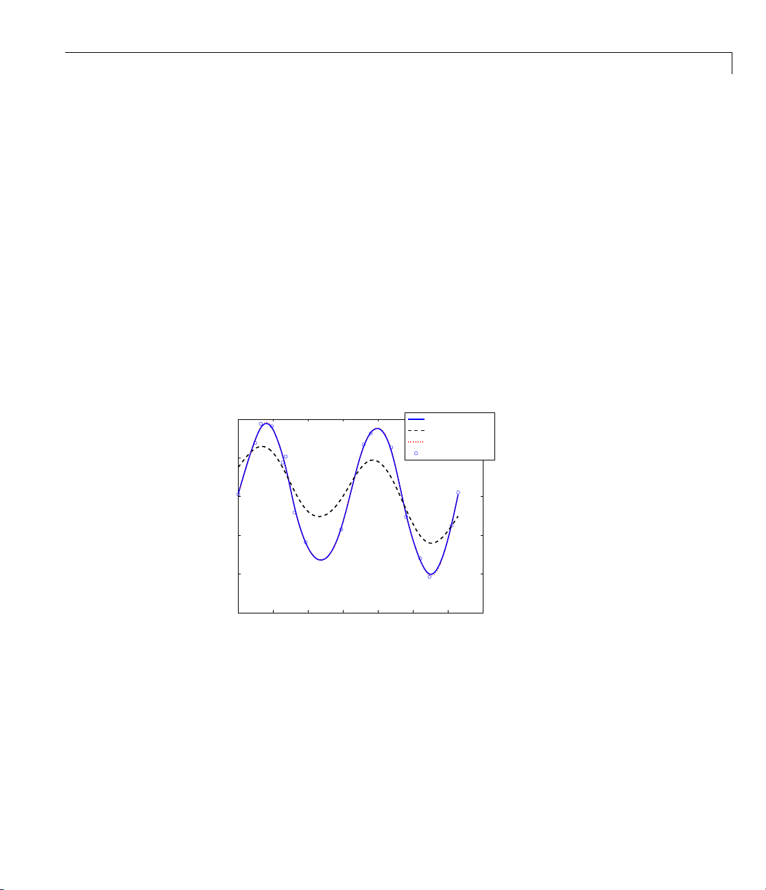
[scs,p] = csaps(x,noisy); fnplt(scs,2), hold on
fnplt(csaps(x,noisy,p/2),2,'k--'), set(gca,'Fontsize',16)
fnplt(csaps(x,noisy,(1+p)/2),2,'r:'), plot(x,noisy,'o')
legend('smoothing spline','more smoothed','less smoothed',...
'noisy data'), hold off

This produces the following picture.

1

0.5

0

−0.5

−1

−1.5
0 2 4 6 8 10 12 14

smoothing spline
more smoothed
less smoothed
noisy data

NoisyDataMoreorLessSmoothed

At times, you might prefer simply to get the smoothest cubic spline sp
that is within a specified tolerance tol of the given data in the sense that

norm(noisy - fnval(sp,x))^2 <= tol. Youcreatethissplinewiththe

command

sp = spaps(x,noisy,tol) foryourdefinedtolerancetol.

2-9

2 Some Simple Examples

Least Squares

If you prefer a le

sp = spap2(knots

k of the sp

order

ast squares approximant, you can obtain it by the statement

line must be provided .

,k,x,y)

; in which both the knot sequence knots and the

The popular ch
have no clear i
polynomial pi

sp = spap2(3,4,x,y);

gives a cubi
error is une
as follows:

sp = spap2(newknt(sp),4,x,y);

oice for the order is 4 , and that gives you a cubic spline. If you

dea of how to choose the knots, simply specify the number of

eces you want used. For example,

c spline consisting of three polynomial pieces. If the resulting

ven, you might try for a better knot distribution by using

newknt

2-10

Using the Spline Fits

You can use the following commands with any example spline, such as the cs,

ch and sp examples constructed in the section “Cubic Spline Interpolation”

on page 2-3.

First construct a spline, for example:

sp = spmak(1:6,0:2)

To display a plot of the spline:

fnplt(sp)

To get the value at a,usethesyntaxfnval(f,a), for example:

fnval(sp,4)

To construct the spline’s second derivative:

Using the Spline Fits

DDf = fnder(fnder(sp))

An alternative way to construct the second derivative:

DDf = fnder(sp,2);

To obtain the spline’s definite integral over an interval [a..b], in this example
from 2 to 5:

diff(fnval(fnint(sp),[2;5]))

To compute the difference between two splines, use the form

fncmb(sp1,'-',sp2), for example:

fncmb(sp,'-',DDf);

2-11

2 Some Simple Examples

Vector-Valued Functions

The toolbox supports vector-valued splines. For example, if you want a spline
curve through given planar points

code defines some data and then creates and plots such a spline curve,
using chord-length parametrization and cubic spline interpolation with the
not-a-knot end condition.

x=[19 43 62 88 114 120 130 129 113 76 135 182 232 298 ...

348 386 420 456 471 485 463 444 414 348 275 192 106 ...
30 48 83 107 110 109 92 66 45 23 22 30 40 55 55 52 34 20 16];

y=[306 272 240 215 218 237 275 310 368 424 425 427 428 ...

397 353 302 259 200 148 105 77 47 28 17 10 12 23 41 43 ...
77 96 133 155 164 157 148 142 162 181 187 192 202 217 245 266 303];

xy = [x;y]; df = diff(xy,1,2);
t = cumsum([0, sqrt([1 1]*(df.*df))]);
cv = csapi(t,xy);
fnplt(cv), hold on, plot(x,y,'o'), hold off

, then the following

2-12

Vector-Valued Functions

If you then wanted to know the area e n clos ed by this curve, you would want to

evaluate the integral
on the curve corresponding to the parameter value

cv just constructed, this can be done exactly in one (somewhat complicated)

,with the point

.Forthesplinecurvein

command:

area = diff(fnval(fnint( ...

fncmb(fncmb(cv,[0 1]),'*',fnder(fncmb(cv,[1 0]))) ...

),fnbrk(cv,'interval')));

To explain, y=fncmb(cv,[0 1]) picks out the second component of the curve
in

cv, Dx=fnder(fncmb(cv,[1 0])) provides the derivative of the first

component, and
Then

IyDx=fnint(yDx) constructs the indefinite integral of yDx and, finally,

yDx=fncmb(y,'*',Dx) constructs their pointwise product.

2-13

2 Some Simple Examples

diff(fnval(IyDx,fnbrk(cv,'interval'))) evaluates that indefinite

integral at the endpoints of the basic interval and then takes the difference of
the second from the first value, thus getting the definite integral of

yDx over

its basic interval. Depending on whether the enclosed area is to the right or to
the left as the curve point travels with increasing parameter, the resulting
number is either positive or negative.

Further, all the values
curve in

cv just constructed can be obtained by the following (somewhat

Y (ifany)forwhichthepoint(X,Y) lies on the spline

complicated) command:

X=250; %Define a value of X
Y = fnval(fncmb(cv,[0 1]), ...

mean(fnzeros(fncmb(fncmb(cv,[1 0]),'-',X))))

To explain: x = fncmb(cv,[1 0]) picks out the first component of the
curve in

= mean(fnzeros(xmX))
is
fncmb(cv,[0,1])

finally,
sites a t which the first component of the curve in

cv; xmX = fncmb(x,'-',X) translates that component by X; t

provides all the parameter values for which xmX

zero, i.e., for which the first component of the curve equals X; y=

picks out the second component of the curve in cv;and,

Y = fnval(y,t) evaluates that second component at those parameter

cv equals X.

As another example of the use of vector-valued functions, suppose that
you have solved the equations of motion of a particle in some specified

force field in the plane, obtaining, at discrete times
the position

4-vector

,asyouwouldif,inthestandardway,youhadsolvedthe

as well as the velocity stored in the

,

equivalent first-order system numerically. Then the following statement,
which uses cubic Hermite interpolation, w ill produce a plot of the particle
path:

fnplt(spapi(augknt(t,4,2),t,reshape(z,2,2*n)).

2-14

Fitting Values at N-D Grid

Vector-valued splines are also used in the approximation to gridded
data, in any number of variables, using tensor-product splines. The

same spline-construction commands are used, only the form of the input
differs. For example, if
of size
satisfying f(x(i),y(j))=z(i,j)fori=1:m, j=1:n. Such a multivariate spline can b e
vector-valued. For example,

gives a perfectly acceptable sphere. Its projection onto the -plane is
plotted by

[m,n],thencs = csapi({x,y},z); describes a bicubic spline f

x = 0:4; y=-2:2; s2 = 1/sqrt(2);
z(3,:,:) = [0 1 s2 0 -s2 -1 0].'*[1 1 1 1 1];
z(2,:,:) = [1 0 s2 1 s2 0 -1].'*[0 1 0 -1 0];
z(1,:,:) = [1 0 s2 1 s2 0 -1].'*[1 0 -1 0 1];
sph = csape({x,y},z,{'clamped','periodic'});
fnplt(sph), axis equal, axis off

Fitting Values at N-D Grid

x is an m-vector, y is an n-vector, and z is an arra y

fnplt(fncmb(sph,[1 0 0; 0 0 1])), axis equal, axis off

Both plots are shown below.

2-15

2 Some Simple Examples

2-16

ASphereMadebya3-D-ValuedBivariateTensorProductSpline

Planar Projection of Spline Sphere

Fitting Values at N-D Grid

2-17

2 Some Simple Examples

Fitting Values at Scattered 2-D Sites

Tensor-product splines are good for gridded (bivariate and even multivariate)
data. For work with scattered bivariate data, the toolbox provides the
thin-plate smoothing spline. Suppose you have given data values
scattered data sites

n = 65; t = linspace(0,2*pi,n+1);
x = [cos(t);sin(t)]; x(:,end) = [0;0];

provides 65 sites, namely 64 points equally spaced on the unit circle, plus the
center of that circle. Here are corresponding data values, namely noisy values
of the very nice function

y = (x(1,:)+.5).^2 + (x(2,:)+.5).^2;
noisy = y + (rand(size(y))-.5)/3;

Then you can compute a reasonable approximation to these data by

st = tpaps(x,noisy);

x(:,j), j=1:N, in the plane. To give a specific examp le ,

y(j) at

.

2-18

and plot the resulting approximation along with the noisy data by

fnplt(st); hold on
plot3(x(1,:),x(2,:),noisy,'wo','markerfacecolor','k')
hold off

and so produce the following picture:

Fitting Values at Scattered 2-D Sites

4

3.5
3

2.5
2

1.5
1

0.5
0

−0.5
1

0.5
0

−0.5

−1

−1

−0.5

0

1

0.5

Thin-Plate Smoothing Spline Approximation to Noisy Data

2-19

2 Some Simple Examples

2-20

Splines: An Overview

• “Introduction” on page 3-2

• “Polynomials vs. Splines” on page 3-3

• “ppform” on page 3-4

• “B-form” on page 3-5

• “Knot Multiplicity” on page 3-6

• “B-Spline Properties” on page 3-7

• “Constructive vs. Variational” on page 3-8

3

• “Multivariate Splines” on page 3-10

• “Rational Splines” on page 3-12

3 Splines: An Overview

Introduction

This chapter provides a quick overview of the mathematics that underlies the
various commands in the Spline Toolbox product. In the process, the technical
terms and notation used throughout this documentation (and in the online
help for individual commands) are introduced. Another source of information
about the latter is the Glossary.

3-2

Polynomials vs. Splines

Polynomials are the approximating f unctions of choice w h en a smooth function
is to be approximated locally. For example, the truncated Taylor series

Polynomials vs. Splines

∑

i

=

n

0

i

xaDfa i

−

()

i

()/ !

provides a satisfactory approximation for f(x) if f is sufficiently smooth and x
is sufficiently close to a. But if a function is to be approximated on a larger
interval, the degree, n, of the approximating polynomial may have to be
chosen unacceptably large. The alternative is to subdivide the interval

[a..b] of approximation into sufficiently small intervals [ξ
ξ

<··· <ξ

1

= b, so that, on each such interval, a polynomial pjof relatively

l+1

..ξ

j

j+1

], with a =

low degree can provide a good approximation to f. This can even be done
in such a way that the polynomial pieces blend smoothly, i.e., so that the
resulting patched or composite function s(x) that equals p

(x) for x [ξjξ

j

j+1

], all
j, has several continuous derivatives. Any such smooth piecewise polynomial
function is called a spline. I.J. Schoenberg coined this term because a twice
continuously differentiable cubic spline with sufficiently small first derivative
approximates the shape of a draftsman’s spline.

There are two commonly used ways to represent a polynomial spline, the
ppform and the B-form. In this toolbox, a spline in ppform is often referred
to as a piecewise polynomial, while a piecewise polynomial in B-form is often
referred to as a spline. This reflects the fact that piecewise polynomials and
(polynomial) splines are just two different views of the same thing.

3-3

3 Splines: An Overview

ppform

The ppform of a poly nomial spline of order k provides a description in terms of
its breaks ξ

px x c j l

jj

Forexample,acubicsplineisoforder 4, corresponding to the fact that
it requires four coefficients to specify a cubic polynomial. The ppform is
convenient for the evaluation and other uses of a spline.

..ξ

1

l+1

k

=−

()

()

∑

=

1

i

and the local polynomial coefficients cjiof its l pieces.

−

ki



=

ji

1,:

3-4

B-form

The B-form has become the standard way to represent a spline during its
construction, because the B-fo rm makes it easy to build in smoothness

requirements across breaks and leads to banded linear systems. The B -form
describes a spline as a weighted sum

n

Ba

∑

jk j

,

1

j

=

of B-splines of the required order k, with their number, n, at least as big as
k–1 plus the number of polynomial pieces that make up the spline. Here, B
B (·|t

, ..., t

j

In particular, B
is nonnegative, is zero outside the interval [t

n

∑

=

1

j

)isthejth B-spline of order k for the knot sequence t1≤t2≤··· ≤t

j+k

Bx ontt

()

jk

is piecewise-polynomial of degree <k,withbreakstj, ... ,t

j,k

=

1

..

[]

+

1

kn,

,..t

],andissonormalizedthat

j

j+k

j,k

n+k

j+k

B-form

=

.
,

3-5

3 Splines: An Overview

Knot Multiplicity

The multiplicity of the knots governs the smoothness, in the following way:
If the number τ occurs exactly r times in the sequence t

,...t

j

,thenB

j+k

and

j,k

its first k-r-1 derivatives are continuous across the break τ,whilethe(k-r)th
derivative has a jump at τ. You can e xperiment with all these properties of the
B-spline in a very visual and interactive way using the command

bspligui.

3-6

B-Spline Properties

B-Spline Properties

Because B

is nonzero only on the interval (tj..t

j,k

), the linear system for

j+k

theB-splinecoefficientsof the spline to be determined, by interpolation or
least squares approximation, or even as the approximate solution of some
differential equation, is banded, making the solving of that linear s ystem
particularly easy. For example, to construct a s pline s of order k with knot
sequence t

n

∑

j

=

1

≤ t2≤··· ≤ t

1

Bxayi n

()

jk

==

ij i,

so that s(xi)=yifor i=1, ..., n, use the linear system

n+k

:

1

for the unknown B-spline coefficients ajinwhicheachequationhasatmostk
nonzero entries.

Also, many theoretical facts concerning splines are most easily stated and/or
proved in terms of B-splines. For example, it is possible to match arbitrary

data at si

,t

,...

(t

n+k

1

Computa

Bx

()

jk

tes

xx

<<

)ifandonlyifB

tions with B-splines are facilitated by stable recurrence relations

xt

−

=

tt

+−

1

jk j

uniquely by a spline of order k with knot sequence

n1

j

Bx

−

)≠0 for all j (Schoenberg-Whitney Conditions).

j,k(xj

tx

−

+

jk

−

1

+

()

tt

jk

++

jk j

Bx

+−

11

−

jk,, ,

1

()

which are also of help in the conversion from B- form to ppform. The dual
functional

ki

−−

as D Ds

=−

:

()

j

( ) () ()

∑

ik

<

1

Ψ

i



j

provides a useful expression for the jth B-spline coefficient of the spline s in
terms of its value and derivatives at an arbitrary site τ between t
with ψ
related to s on the interval [t

(t):=(t

j

–t)··· (t

j+1

–t)/(k–1)! Itcanbeusedtoshowthataj(s)isclosely

j+k–1

..t

], and seems the most efficient means for

j

j+k

and t

j

j+k

,and

converting from ppform to B-form.

3-7

3 Splines: An Overview

Constructive vs. Variational

The above constructive approach is not the only avenue to splines. In the
variational approach, a spline is obtained as a best interpolant, e.g., as the

function with smallest mth derivative among all those matching prescribed
function values at certain sites. As it turns out, among the many such
splines available, only those that are piecewise-polynomials or, perhaps,
piecewise-exponentials have found much use. Of particular practical interest
is the smoothing spline s = s

i, and given corresponding positive weights w
parameter p, minimizes

which, for given data (xi,yi)withx [a..b], all

p

,andforgivensm oothing

i

pwy fx p Dftdt

∑

over all functions f with m derivatives. It turns out that the smoothing spline
s is a spline of order 2m with a break at every data site. The smoothing

parameter, p, is chosen artfully to strike the right balance between wanting
the error measure

Es w y sx

()

small and wanting the roughness measure

FD s D st dt

()

small. Thehopeisthats contains as much of the information, and as little
of the supposed noise, in the data as possible. One approach to this (used in

spaps)istomakeF(D

be no bigger than a prescribed tolerance. For computational reasons,
uses the (equivalent) smoothing parameter ρ=p/(1–p), i.e., minimizes ρE(f)+

m

F(D

f). Also, it is useful at times to use the more flexible roughness measure

−

iiii

=−

∑

i

mm

=

2

+−

()

ii i

∫

()

b

()

a

m

1()

()

2

f) as small as possible subject to the condition that E(f)

b

∫

a

2

2

m

spaps

3-8

mm

FD s tD st dt

()

b

=



()

∫

a

2

()

with λ a suitable positive weight function.

Constructive vs. Variational

3-9

3 Splines: An Overview

Multivariate Splines

Multivariate splines can be obtained from univariate sp li n es by the tensor
product construct. For example, a trivariatesplineinB-formisgivenby

U

fxyz B xB yB za

,,

()

=

∑∑∑

wWvVu

() () ()

uk vl wm uvw

,,, ,,

===

111

with B
order k in x,oforderl in y,andoforderm in z. Similarly, the ppform of a
tensor-product spline is specified by b reak sequences in each o f the variables
and, fo r each hyper-rectangle thereby specified, a coefficient array. Further,
as in the univariate case, the coefficients may be vectors, typically 2-vectors
or 3-vectors, making it possible to represent, e.g., certain surfaces in ℜ

A very different bivariate spline is the thin-plate spline.Thisisafunctionof
the form

with ψ(x)=|x|2log|x|2the thin-plate spline basis function, and |x|denoting
the Euclidean length of the vector x. Here, for convenience, denote the
independent variable by x,butx is now a vector whose two components, x(1)
and x(2),playtheroleofthetwoindependent variables earlier denoted x and
y. Correspondingly, the sites c

Thin-plate splines arise as biv ariate smoothing splines, meaning a thin-plate
spline minimizes

u,k,Bv,l,Bw,m

n

−

fx x c a x a x a a

=−

()

∑

j

=

3

−

n

pyfc pDDf DDf DDf

−+−

∑

ii

1

=

i

univariate B -splines. Correspondingly, this spline is of

3

Ψ 12

()

1

2

()

+

jj n n n

12

()

11

(

∫

+

()

−−

21

are points in ℜ2.

j

2

++

2

12

+

2

22

)

3

.

3-10

over all sufficiently smooth functions f. Here, the yiare data values given at
the data sites c
derivative of f with respect to x(j). The integral is taken over the entire ℜ

, p is the smoothing parameter, and Djf denotes the partial

i

2

.

Multivariate Splines

The upper summation limit, n–3, reflects the fact that 3 degrees of freedom of
thethin-platesplineareassociatedwithitspolynomialpart.

Thin-plate splines are functions in stform, meaning that, up to certain
polynomial terms, they are a weighted sum of arbitrary or scattered translates
Ψ(·-c)ofonefixedfunction,Ψ. This so-called basis function for the thin-plate
spline is special in that it is radially symmetric, meaning that Ψ(x)only
depends on the Euclidean length, |x|, of x. For that reason, thin-plate splines
are also known as RBFs or radial basis functions. See Chapter 8, “The stform”
for more information.

3-11

3 Splines: An Overview

Rational Splines

A rational spline is any function of the form r(x)=s(x)/w(x), with both s
and w splines and, in particular, w a scalar-val u ed spline, while s often
is vector-valued.

Rational splines are attractive because it is possible to describe various basic
geometric shapes, like conic sections, exactly as the range of a rational spline.
For example, a circle can so be described by a quadratic rational spline with
just two pieces.

In this toolbox, there is the additional requirement that both s and w be of
the same form and even of the same order, and with the same knot or break
sequence. Thismakesitpossibletostoretherationalspliner as the ordinary
spline R whose value at x is the vector [s(x);w(x)]. Depending on whether the
two splines are in B-form or ppform, such a representation is called here the
rBform or the rpform of such a rational spline.

It is easy to obtain r from R. For example, if

v(1:end-1)/v(end) is the value of r at x. There are corresponding ways to

express derivatives of r in terms of derivatives of R.

v is the value of R at x,then

3-12

The ppform

• “Introduction” on page 4-2

• “ppform” on page 4-3

• “Construction” on page 4-4

• “Available Commands” on page 4-6

4

4 The ppform

Introduction

Aunivariatepiecewise polynomial f is specified by its break sequence breaks
and the coefficient array coefs of the local power form (see Equation 4-1
below) of its polynomial pieces; see Chapter 6, “Tensor Product Splines” for
a discussion of multivariate piecewise-polynomials. The coefficients may
be (column-)vectors, matrices, even ND-arrays. For simplicity, the present
discussion deals only with the cas e when the coefficients are scalars.

The break sequence is assumed to be strictly increasing,

breaks(1)
< breaks(2) < ... < breaks(l+1)

with l the number of polynomial pieces that make up f.

While these polynomials may be of varying degrees, they are all recorded as
polynomials of the same order

[l,k],withcoefs(j,:) containing the k coefficients in the local power

form for the
Equation 4-1 below.

jth polynomial piece, from the highest to the lowest power; see

k, i.e., the coefficient array coefs is of size

4-2

ppform

The items breaks, coefs, l,and k,makeuptheppform of f, along with the
dimension
form is the interval [
over which a function in ppform is plotted by the plot command

In these terms, the precise description of the piecewise-polynomial f is

d of its coefficients; usually d equals 1. The basic interval of this

breaks(1) .. breaks(l+1)]. It is the default interval

fnplt.

ppform

f(t) = polyval(coefs(j,:), t - breaks(j))

for breaks(j)≤t<breaks(j+1).

Here,

polyval(a,x) is the MATLAB function; it returns the number

k

∑

j

=

1

This defines f(t) only for t in the half-open interval [breaks(1)..breaks(l+1)).
For any other t, f(t) is defined by

f t polyval coefs j t breaks j j

()

i.e., by extending the first, respectively last, polynomial piece. In this way, a
function in ppform has possible jumps, in its value a nd/or its derivatives, only
across the interior b reaks,
mainly serve to define the bas ic interval of the ppform.

kj k k

ajx a x a x akx

−−−

()

=

=

()

12 0

12

()

+

()

−

,: ,

()

breaks(2:l).Theendbreaks,breaks([1,l+1]),

++

...

()

()

=

lt bre

t breaks

<

,,11

≥

()

aaks l +

1

()

(4-1)

4-3

4 The ppform

Construction

A piecewise-polynomial is usually constructed by some command, through a
process of interpolation or approximation, or conversion from some other form
e.g., f rom the B-form, and is output as a v ariable. But it is also possible to
make one up from scratch, using the statement

pp
= ppmak(breaks,coefs)

For e xample, if you enter pp=ppmak(-5:-1,-22:-11), or, more explicitly,

breaks = -5:-1;
coefs = -22:-11; pp = ppmak(breaks,coefs);

you specify the uniform break sequence -5:-1 and the coefficient sequence

-

22:-11. Because this break sequence has 5 entries, hence 4 break intervals,

while the coefficient sequence has 12 entries, you have, in effect, specified a
piecewise-polynomial of order 3 (= 12/4). The command

4-4

fnbrk(pp)

prints out all the constituent parts of this piecewise-polynomial, as follows:

breaks(1:l+1)

-5 -4 -3 -2 -1

coefficients(d*l,k)

-22 -21 -20

-19 -18 -17

-16 -15 -14

-13 -12 -11

pieces number l

4

order k

3

dimension d of target

1

Further, fnbrk canbeusedtosupplyeachofthesepartsseparately. But
the point of Spline Toolbox is that you usually need not concern yourself
with these d etails. You simply use

pp as an argument to commands that

evaluate, differentiate, integrate, convert, or plot the piecewise-polynomial
whose description is contained in

pp.

Construction

4-5

4 The ppform

Available Commands

Here are some operations you can perform on a piecewise-polynomial.

v = fnval(pp,x)

dpp = fnder(pp)

dirpp = fndir(pp,dir)

ipp = fnint(pp)

fnmin(pp,[a,b])

Evaluates

Differentiates

Differentiates in the direction dir

Integrates

Finds the minimum value in given
interval

fnzeros(pp,[a,b])

pj = fnbrk

pc = fnbrk(pp,[a b])

po = fnxtr(pp,order)

(pp,j)

Finds the z

Pulls out the jth polynomial piece

Restricts/extends to the interval
[

a..b]

Extend
polyn

(pp,[a,b])

fnplt

sp = fn2fm(pp,'B-')

pr = fnrfn(pp,morebreaks)

serting additional breaks comes in handy when you want to add two

In

ecewise-polynomials with different breaks, as is done in the command

pi

Plots on given interval

Converts to B-form

Inserts additional breaks

eros in the given interval

s outside its basic interval by

omial o f specified order

fncmb.

4-6

illustrate the use of some of these commands, execute the following

To

ommandstocreateandplottheparticular piecewise-polynomial described in

c

he “Construction” on page 4-4 section.

t

reate the piecewise-polynomial with break sequence

1 C

sequence

pp=ppmak(-5:-1,-22:-11)

2 Create the basic plot:

-22:-11:

-5:-1 and coefficient

Available Commands

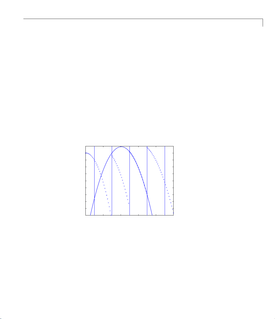
x = linspace(-5.5,-.5,101);
plot(x, fnval(pp,x),'x')

3 Add the break lines to the plot:

breaks=fnbrk(pp,'b'); yy=axis; hold on
for j=1:fnbrk(pp,'l')+1

plot(breaks([j j]),yy(3:4))

end

4 Superimpose the plot of the polynomial that supplies the third polynomial

piece:

plot(x,fnval(fnbrk(pp,3),x),'linew',1.3)
set(gca,'ylim',[-60 -10]), hold off

−10

−15

−20

−25

−30

−35

−40

−45

−50

−55

−60

−5.5 −5 −4.5 −4 −3.5 −3 −2.5 −2 −1.5 −1 −0.5

A Piecewise-Polynomial Function, Its Breaks, and the Polynomial Giving
Its Third Piece

The figure above is the final picture. It shows the piecewise-polynomial as
a sequence of points and, solidly on top of it, the polynomial from which its
third polynomial piece is taken. It is quite noticeable that the value o f a
piecewise-polynomial at a bre ak is its limit from the right, and that the value
of the piecewise-polynomial outside its basic interval is obtained by extending
its leftmost, respectively its rightmost, polynomial piece.

4-7

4 The ppform

While the ppform of a piecewise-polynomial is efficient for evaluation, the
construction of a piecewise-polynomial from some data is usually more
efficiently handled by determining first its B-form, i.e., its representation
as a linear combination of B-splines.

4-8

The B-form

• “Introduction” on page 5-2

• “B-form” on page 5-3

• “B-Splines” on page 5-4

• “Knot Multiplicity” on page 5-5

• “Choice of Knots” on page 5-7

• “Splines” on page 5-8

• “Construction” on page 5-9

5

• “Example: A Spline Curve” on page 5-10

• “Available Commands” on page 5-12

5 The B-form

Introduction

A univariate spline f is specified by its nondecreasing knot sequence t
and by its B-spline coefficient sequence a. See Chapter 6, “Tensor Product
Splines” for a discussion of multivariate spli nes. The coefficients may be
(column-)vectors, matrices, even ND-arrays. When the coefficients are
2-vectors or 3-vectors, f is a curve in R
the control points for the curve.

Roughly speaking, such a spline is piecewise-polynomial of a certain order
and with breaks
may be repeated, i.e.,
multiplicities govern the smoothness of the spline across the knots, as detailed
below.

With

[d,n] = size(a),and n+k = length(t), the sp line is of order k.This

means that its polynomial pieces have degree <
spline is a spline of order 4 because it takes four coefficients to specify a cubic
polynomial.

t(i). But knots are different from breaks in that they

t need not be strictly increasing. The resulting knot

2

or R3and the coefficients are called

k. For example, a cubic

5-2

B-form

These four items, t, a, n,andk,makeuptheB-formofthesplinef.

This means, explicitly, that

n

fBai

=

∑

i

=

1

ik

,

:,

()

B-form

with B

t,i.e.,theB-splinewithknotst(i),...,t(i+k). The basic interval of this B-form

=B(·|t(i:i+k)) the ith B-spline of order k for the given knot sequence

i,k

is the interval [t(1)..t(n+k)]. It is the default interval over which a spline in
B-form is plotted by the command
outside its basic interval while, after conversion to ppform via

fnplt. Note that a spline in B-form is zero

fn2fm,thisis

usually not the case because , outside its basic interval, a piecew ise-polynomial
is defined by extension of its first or last polynomial piece. In particular, a
function in B-form may have jumps in value and/or one of its derivative not
only across its interior knots, i.e., across t(i)witht(1)<t(i)<t(n+k),butalso
across its end knots, t(1) and t(n+k).

5-3

5 The B-form

B-Splines

The building blocks for the B-form of a spline are the B-splines. A B-Spline
of Order 4, and the Four Cubic Polynomials from Which It Is Made on page
5-4 shows a picture of such a B-spline, the one with the knot sequence

1.5 2.3 4 5]

make up the B-spline. The information for that picture could be generated
by the command

bspline([0 1.5 2.3 4 5])

, hen ce of order 4, together with the polynomials whose pieces

[0

5-4

A B-Spline of Order 4, and the Four Cubic Polynomials from Which It Is Made

To summarize: The B-spline with knots t(i)≤····≤ t(i+k)ispositiveonthe
interval (t(i)..t(i+k))and is zero outside that interval. It is piecewise-polynomial
of order
and the precise multiplicity governs the smoothness with which the two
polynomial pieces join there.

k with breaks at the sites t(i),...,t(i+k). These knots may coincide,

Knot Multiplicity

Theruleis

knot multiplicity + condition m ultiplicity = order

Knot Multiplicity

All Third-Order B-Splines for a Certain Knot Sequence with Various Knot
Multiplicities

For example, for a B-spline of order 3, a simple knot would mean two
smoothness conditions, i.e., continuity of function and first derivative, while a
double knot would only leave one smoothness condition, i.e., just continuity,
and a triple knot would leave no smoothness condition, i.e., even the function
would be discontinuous.

All Third-Order B-Splines for a Certain Knot Sequence with Various Knot
Multiplicities on page 5-5 shows a picture of all the third-order B-splines
for a certain mystery knot sequence
lines. F or each break, try to determine its multiplicity in the knot sequence
(it is 1,2,1,1,3), as well as its multiplicity as a knot in each of the B-splines.
For example, the second break has multiplicity 2 but appears only with
multiplicity 1 in the third B-spline and not at all, i.e., with multiplicity 0, in
the last two B-splines. Note that only one of the B-splines shown has all its
knots simple. It is the only o ne having three different nontrivial polynomial
pieces. Note also that you can tell the knot-sequence multiplicity of a knot

t. The breaks are indicated by vertical

5-5

5 The B-form

by the number of B-splines whose nonzero part begins or ends there. The
picture is generated by the following MATLAB statements, which use the
command
B-splines at a fine net

t=[0,1,1,3,4,6,6,6]; x=linspace(-1,7,81);
c=spcol(t,3,x);[l,m]=size(c);
c=c+ones(l,1)*[0:m-1];
axis([-1 7 0 m]); hold on
for tt=t, plot([tt tt],[0 m],'-'), end
plot(x,c,'linew',2), hold off, axis off

spcol from this toolbox to generate the function values of all these

x.

Further illustrated examples are provided by the demo “Intro to B-form”
available on the Demos tag in the MATLAB Help browser. You can also
use the GUI

bspligui to study the dependence of a B-spline on its knots

experimentally.

5-6

Choice of Knots

The rule “knot m ultiplicity + condition multiplicity = order” has the following
consequence for the process of choosing a knot sequence for the B-form of
a spline approximant. Suppose the spline s is to be of order k, with basic
interval [a..b], and with interior breaks ξ

ξ

, the spline is to satisfy μismoothness conditions, i.e.,

i

Choice of Knots

<···<ξl. Suppose, further, that, at

2

jump Ds Ds Ds j i l

jjij

: , , ,...,=



i

()−()

 

+−

=≤< =

00 2

ii

Then, the appropriate knot sequence t should contain the break ξiexactly k –
μ

times, i=2,...,l. In addition, it should contain the two endpoints, a and b,of

i

the basic interval exactly k times. This last requirement can be relaxed, but
has become standard. With this choice, there is exactly one w a y to write each
spline s with the properties described as a weighted sum of the B-splines of
order k with knots a segment of the knot sequence t. This is the reason for the
B in B-spline: B-splines are, in Schoenberg’s terminology, basic splines.

For example, if you want to generate the B-form of a cubic spline on the
interval [1 .. 3], with interior breaks 1.5, 1.8, 2.6, and with two continuous
derivatives, then the following would be the appropriate knot sequence:

t = [1, 1, 1, 1, 1.5, 1.8, 2.6, 3, 3, 3, 3];

This is supplied by augknt([1, 1.5, 1.8, 2.6, 3], 4). If you wanted,
instead, to allow for a corner at 1.8, i.e., a possible jump in the first derivative
there, you would triple the knot 1.8, i.e., use

t = [1, 1, 1, 1, 1.5, 1.8, 1.8, 1.8, 2.6, 3, 3, 3, 3];

andthisisprovidedbythestatement

t = augknt([1, 1.5, 1.8, 2.6, 3], 4, [1, 3, 1] );

5-7

5 The B-form

Splines

The shorthand

fS

kt∈,

is one of several ways to indicate that f is a spline of ord er k with knot sequence

t, i.e., a linear combination of the B-splines of order k for the knot sequence t.

A word of caution: The term B-spline has been expropriate d by the
Computer-Aided Geometric Design (CAGD) community to mean what is
called here a spline in B-form, with the unhappy result that, in any discussion
between m athematicians/approximation theorists and people in CAGD, one
now always has to check in what sense the term is being used.

5-8

Construction

Construction

Usually, a spline is constructed from some information, like function values
and/or derivative values, or as the approximate solution of som e ordinary
differential equation. But it is also possible to make up a spline from scratch,
by providing its knot sequence and its coefficient sequence to the command

spmak.

For example, if you enter

sp = spmak(1:10,3:8);

you supply the uniform knot sequence 1:10 and the coefficient sequence 3:8.
Because there are 10 knots and 6 coefficients, the order must be 4(= 10 – 6),
i.e., you get a cubic spline. The command

fnbrk(sp)

prints out the constituent parts of the B-form of this cubic spline, as follows:

knots(1:n+k)

12345678910

coefficients(d,n)

345678

number n of coefficients

6

order k

4

dimension d of target

1

Further, fnbrk canbeusedtosupplyeachofthesepartsseparately.

But the point of the Spline Toolbox product is that there shouldn’t be any
need for you to look up these details. You simply use

sp as an argument to

commands that evaluate, differentiate, integrate, convert, or plot the spline
whose description is contained in

sp.

5-9

5 The B-form

Example: A Spline Curve

As another simple example,

points = .95*[0 -1 0 1;1 0 -1 0];
sp = spmak(-4:8,[points points]);

provides a planar, quartic, spline curve whose middle part is a pretty good
approximation to a circle, as the plot on the next page shows. It is generated
by a subsequent

plot(points(1,:),points(2,:),'x'), hold on
fnplt(sp,[0,4]), axis equal square, hold off

Insertion of additional control points

±±

095 095 19., . / .

()

would make a

visually perfect circle.

Here are more details. The spline curve generated has the form Σ
j), with -

4:8 the uniform knot sequence, and with its control points a(:,j)the

8

B

a(:,

j=1

j,5

sequence (0,α),(–α,0),(0,–α),(α,0),(0,α),(–α,0),(0,–α),(α,0) with α=0.95. Only the
curve part between the parameter values 0 and 4 is actually plotted.

To get a feeling for how close to circular this part of the curve actually is,
compute its unsigned curvature. The curvature κ(t) at the curve point γ(t)=
(x(t), y(t)) of a space curve γ can be computed from the formula

=

+

xy

(’ ’)

/2232

−

xy yx

’’’ ’’’



in which x’, x″, y’, and y” are the first and second derivatives of the curve with
respect to the parameter used (t). Treat the planar curve as a space curve in
the (x,y)-plane, hence obtain the maximum and minimum of its curvature at
21 points as follows:

t = linspace(0,4,21);zt = zeros(size(t));
dsp = fnder(sp); dspt = fnval(dsp,t); ddspt = fnval(fnder(dsp),t);
kappa = abs(dspt(1,:).*ddspt(2,:)-dspt(2,:).*ddspt(1,:))./...

(sum(dspt.^2)).^(3/2);

[min(kappa),max(kappa)]

5-10

Example: A Spline Curve

ans =

1.6747 1.8611

So, while the curvature is not quite constant, it is close to 1/radius of the
circle, as you see from the next calculation:

1/norm(fnval(sp,0))

ans =

1.7864

1

x

0.8

0.6

0.4

0.2

x

0

x

-0.2

-0.4

-0.6

-0.8

-1

-1 -0.5 0 0.5 1

x

Spline Approximation to a Circle; Control Points Are Marked x

5-11

5 The B-form

Available Commands

Thefollowingcommandsareavailableforsplinework. Thereisspmak and

fnbrk to make up a spline and take it apart again. Use fn2fm to convert from

B-form to ppform. You can evaluate, differentiate, integrate, minimize, find
zeros of, plot, refine, or selectively extrapolate a spline with the aid of

fnder, fndir, fnint, fnmin, fnzeros, fnplt, fnrfn,andfnxtr.

There are five commands for generating knot sequences:

•

augknt for providing boundary knots and also controlling the multiplicity

of interior knots

•

brk2knt for supplying a knot sequence with specified multiplicities

aptknt for providing a knot sequence for a spline space of given order that

•

is suitable for interpolation at given d ata sites

•

optknt for providing an optimal knot sequence for interpolation at given

sites

fnval,

5-12

•

newknt for a knot sequence perhaps more suitable for the function to be

approximated

In addition, there is:

•

aveknt to supply certain knot averages (the Greville sites) as recommended

sites for interpolation

•

chbpnt to supply such sites

knt2brk and knt2mlt for extracting the breaks and/or their multiplicities

•

from a given knot sequence

To display a spline curve with given two-dimensional coefficient sequence and
a uniform knot sequence, use

spcrv.

You can also write your own spline construction commands, in which
case you will need to know the following. The construction of a spline
satisfying some interpolation or approximation conditions usu al ly requires a
collocation matrix, i.e., the matrix that, in each row, contains the sequence
of numbers D
all j,forsomer and some site τ. Such a matrix is provided by

r

B

(τ), i.e., the rth derivative at τ of the jth B-spline, for

j,k

spcol.An

Available Commands

optional argument allows for this matrix to be supplied by spcol in a
space-saving spline-almost-block-diagonal-form or as a MATLAB sparse
matrix. It can be fed to

slvblk, a command for solving lin ea r systems with

an almost-block-diagonal coefficient matrix. If you are interested in seeing
how

spcol and slvblk are used in this toolbox, have a look at the commands

spapi, spap2,andspaps.

In addition, there are routines for constructing cubic splines.

csape provide the cubic spline interpolant at knots to given data, using the

csapi and

not-a-knot and various other end conditions, respectively. A parametric cubic
spline curve through given points is provided by
spline is constructed in

csaps.

cscvn.Thecubicsmoothing

The remaining commands involving the B-form are utilities, of no interest to
the casual user.

5-13

5 The B-form

5-14

Tensor Product Splines

• “Introduction” on page 6-2

• “B-form” on page 6-3

• “Construction and Use” on page 6-4

• “ppform” on page 6-5

• “Example: The Mobius Band” on page 6-6

6

6 Ten s or Pro duct S p lin e s

Introduction

The toolbox provides (polynomial) spline functions in any number of variables,
as tensor products of univariate splines. These multivariate splines come in
both standard forms, the B-form and the ppform, and their construction and
use parallels entirely th at of the univariate splines discussed in previous
sections, Chapter 4, “The ppform” and Chapter 5, “The B-form” The same
commands are used for their construction and use.

For simplicity, the following discussion deals just with bivariate splines.

6-2

B-form

The tensor-product idea is very simple. If f is a function of x,andg is a
function of y, then their tensor-product p (x,y): = f (x)g(y) is a function of x and
y, i.e., a bivariate function. More gen erally, with s=(s
knot sequences and a

:i=1,...,m;j=1,...n) a corresponding coefficient array, you

ji

,...,s

1

)andt=(t1,...,t

m+h

n+k

obtain a bivariate spline as

m

fxy Bx s s By t t a

( , ) | ,..., | ,...,=

()

∑∑

11

jni

==

iih j jkij

()

++

TheB-formofthissplinecomprisesthecellarray{s,t}ofitsknotsequences,
the coefficient array a, the numbers vector [m,n], and the orders vector [h,k].
The command

sp = spmak({s,t},a);

constructs this form. Further, fnplt, fnval, fnder, fndir, fnrfn,andfn2fm
canbeusedtoplot,evaluate,differentiate and integrate, refine, and convert
this form.

B-form

)

6-3

6 Ten s or Pro duct S p lin e s

Construction and Use

You are most likely to construct such a form by looking for an interpolant
or approximant to gridded data. For example, if you know the values
z(i,j)=g(x(i),y(j)),i=1:m, j=1:n,ofsomefunctiong at all the points in a
rectangular grid, then, assuming that the strictly increasing sequence
satisfies the Schoenberg-Whitney conditions with respect to the above
knot sequence s, and that the strictly increasing sequence
Schoenberg-Whitney conditions with respect to the above knot sequence
t, the command

sp=spapi({s,t},[h,k],{x,y},z);

constructs the unique bivariate spline of the above form that matches
the given values. The command
interpolant. The command
this spline, which is probably what you w ant when y ou want to evaluate the
spline at a fine grid (

x

y satisfies the

fnplt(sp) gives you a quick plot of this

pp = fn2fm(sp,'pp') gives you the ppform of

(xx(i),yy(j)) for i=1:M, j=1:N), by the com mand:

6-4

values = fnval(pp,{xx,yy});

ppform

Theppformofsuchabivariatesplinecomprises, analogously, a cell array of
break sequences, a multidimensional coefficient array, a vector of number
pieces, and a vector of polynomial orders. Fortunately, the toolbox is set up
in such a way that there is usually no reason for you to concern yourself
with these details of either form. You use interpolation, approximation, or
smoothing to construct splines, and then use the
use of them.

fn... commands to make

ppform

6-5

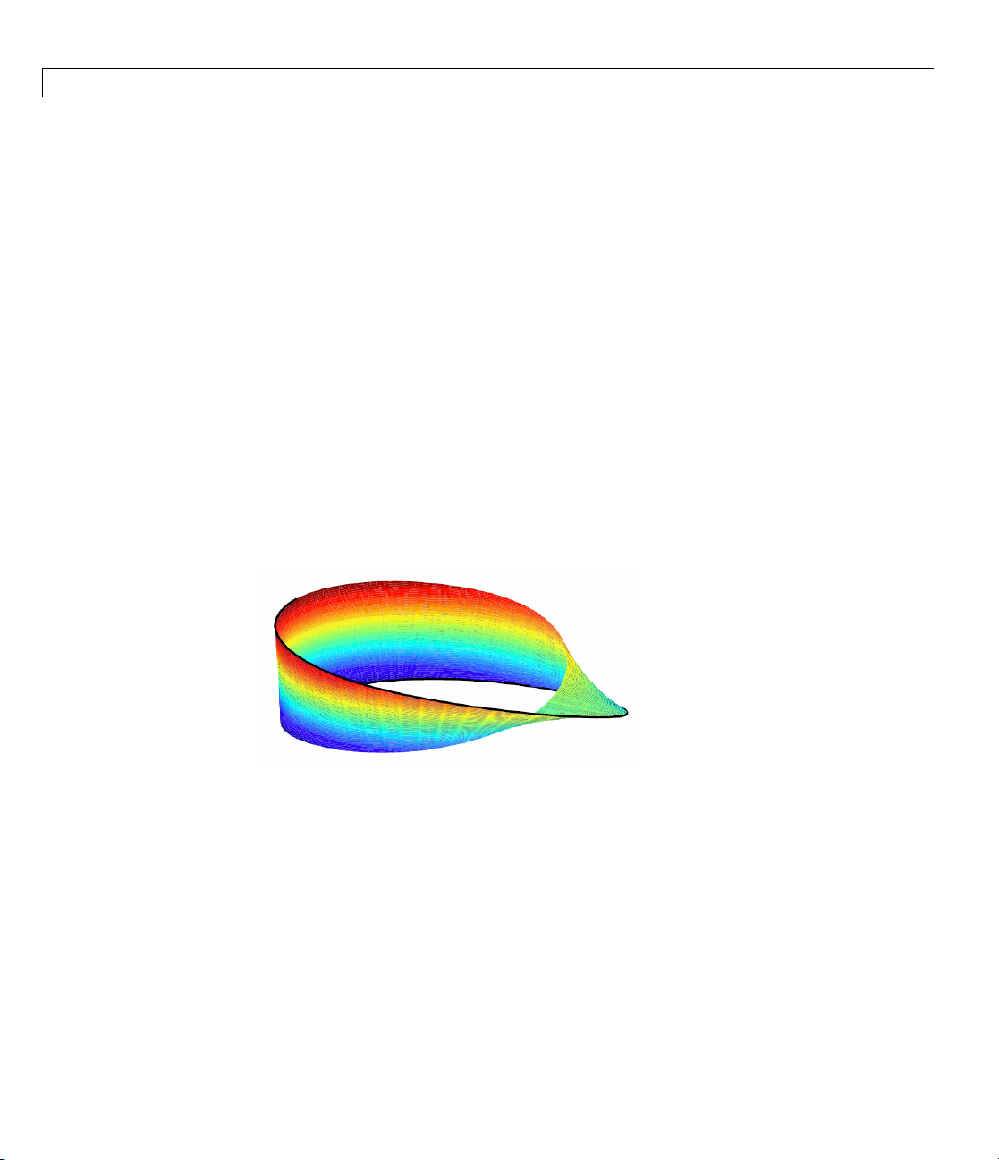
6 Ten s or Pro duct S p lin e s

Example: The Mobius Band

Here is an example of a surface constructed as a 3-D-valued bivariate spline.
ThesurfaceisthefamousMöbiusband,obtainable by taking a longish strip
of paper and gluing its narrow ends together, but with a twist. The figure is
obtained by the following commands:

x = 0:1; y = 0:4; h = 1/4; o2 = 1/sqrt(2); s = 2; ss = 4;
v(3,:,:) = h*[0, -1, -o2, 0, o2, 1, 0;0, 1, o2, 0, -o2, -1, 0];
v(2,:,:) = [ss, 0, s-h*o2, 0, -s-h*o2, 0, ss;...

v(1,:,:) = s*[0, 1, 0, -1+h, 0, 1, 0; 0, 1, 0, -1-h, 0, 1, 0];
cs = csape({x,y},v,{'variational','clamped'});
fnplt(cs), axis([-2 2 -2.5 2.5 -.5 .5]), shading interp
axis off, hold on
values = squeeze(fnval(cs,{1,linspace(y(1),y(end),51)}));
plot3(values(1,:), values(2,:), values(3,:),'k','linew',2)
view(-149,28), hold off

ss, 0, s+h*o2, 0,-s+h*o2, 0, ss];

6-6

A Möbius Band Made by Vector-Valued Bivariate Spline Interpolation

7

NURBS and Other Rational
Splines

• “Introduction” on page 7-2

• “Example: Circle” on page 7-3

• “Example: Sphere” on page 7-5

• “rsform: rpform, rBform” on page 7-6

• “Available Commands” on page 7-8

7 NURBS and Other Rational Splines

Introduction

A rational spline is, by definition, any function that is the ratio of two splines:

rx sx wx

()=() ()

This requires w to be scalar-valued, but s is often chosen to be vector-valued.
Further, it is desirable that w(x)benotzeroforanyx of interest.

Rational splines are popular because, in contrast to ordinary splines, they can
be used to describe certain basic design shapes, like conic sections, exactly.

/

7-2

Example: Circle

For example,

circle = rsmak('circle');

provides a rational spline whose values on its basic in terval trace out the uni t
circle, i.e., the circle of radius 1 with center at the origin, as the command

fnplt(circle), axis square

readily show s; the resulting output is the circle in the figure A Circle and an
Ellipse, Both Given by a Rational Spline on page 7-4.

It is easy to manipulate this circle to obtain related shapes. For example, the
next commands stretch the circle into an ellipse, rotate the ellipse 45 degrees,
and translate it by (1,1), and then plot it on top of the circle.

ellipse = fncmb(circle,[2 0;0 1]);
s45 = 1/sqrt(2);
rtellipse = fncmb(fncmb(ellipse, [s45 -s45;s45 s45]), [1;1] );
hold on, fnplt(rtellipse), hold off

Example: Circle

As a further example, the "circle" just constructed is put together from four
pieces. To highlight the first such piece, use the following commands:

quarter = fnbrk(fn2fm(circle,'rp'),1);
hold on, fnplt(quarter,3), hold off

In the first command, fn2fm is used to change forms, from one based on the
B-form to one based on the ppform, and then

fnbrk is used to extract the

first piece, and this piece is then plotted on top of the circle in A Circle and
an Ellipse, B oth Given by a Rational Spline on page 7-4, with linewidth

3

to make it stand out.

7-3

7 NURBS and Other Rational Splines

−1 −0.5 0 0.5 1 1.5 2 2.5 3

−1

−0.5

0

0.5

1

1.5

2

2.5

3

A Circle and an Ellipse, Both Given by a Rational Spline

7-4

Example: Sphere

As a surface example, the command rsmak('southcap') provides a 3-vector
valued rational bicubic polynomial whose values on the unit square [-1 .. 1]^2
fill out a piece of the unit sphere. Adjoin to it five suitable rotates of it and
you get the unit sphere exactly. For illustration, the following commands
generate tw o-thirds of that sphere, as shown in Part of a Sphere Formed by
Four Rotates of a Quartic Rational on page 7-5.

southcap = rsmak('southcap'); fnplt(southcap)
xpcap = fncmb(southcap,[0 0 -1;0 1 0;1 0 0]);
ypcap = fncmb(xpcap,[0 -1 0; 1 0 0; 0 0 1]);
northcap = fncmb(southcap,-1);
hold on, fnplt(xpcap), fnplt(ypcap), fnplt(northcap)
axis equal, shading interp, view(-115,10), axis off, hold off

Example: Sphere

Part of a Sphere Formed by Four Rotates of a Quartic Rational

7-5

7 NURBS and Other Rational Splines

rsform: rpform, rBform

Offhand, the two splines, s and w, in the rational spline r(x)=s(x)/w(x) need
not be related to one another. They could even be of different forms. But,
in the context of this toolbox, it is convenient to restrict them to be of the
same form, and even of the same order and with the same breaks or knots.
For, under that assumption, you can represent such a rational spline by the
(vector-valued) spline function

Rx sx wx

whose values are vectors with one more entry than the values of the rational
spline r, and call this the rsform of the rational spline, or, more precisely, the
rpform or rBform, depending on whether s and w are in ppform or in B-form.
Internally, the only thing that distinguishes these rational forms from their
corresponding ordinary spline forms, rpform and B-form, is their form part,
i.e., the string obtained via

fn... commands to act appropriately on a function in one of the rsforms.

Forexample,asisdonein
is the value of R at x, then v(1:end-1)/v(end) is the value of r at x.If,in
addition,
Dr(x). More generally, by Leibniz’s formula,

Ds D wr

Therefore,

Dr Ds

⎡

()=() ()

⎣

dv is DR(x), then (dv(1:end-1)-dv(end)*v(1:end-1))/v(end) is

jj

=

()

⎛

jj iji

⎜

=−

⎜
⎝

;

∑

i

⎤

⎦

j

j

⎛

=

⎜

∑

i

⎝

i

=

0

j

j

⎛

⎞

DwD r w

⎜

⎟

i

⎝

⎠

=

1

fnbrk(r,'form'). This is enough to alert the

fnval, it is very easy to obtain r(x)fromR(x). If v

⎞

iji

DwD r

⎟
⎠

−

⎞

−

⎟

/

⎟
⎠

7-6

This shows that you can compute the derivatives of r inductively, using the
derivatives of s and w (i.e., the derivatives of R) along with the derivatives of r
of order less than j to compute the jth derivative of r. This inductive scheme
is used in

fntlr to provide the first so many derivative s of a rational spline.

rsform: rpform, rBform

There is a corresponding formula for partial and directional derivatives for
multivariate rational splines.

7-7

7 NURBS and Other Rational Splines

Available Commands

Having chosen to represent the rational spline r = s/w inthiswaybythe
ordinary spline R=[s;w] makes it is easy to apply to a rational spline all the

fn... commands in the Spline Toolbox product, with the following exceptions.

The integral of a rational spline need not be a rational spline, hence there
is no way to extend
spline is again a rational spline but one of roughly twice the order. For that
reason,
command
to a given order of a given function. If that function is rational, the needed
calculation is based on the considerations given in the preceding paragraph.

fnint to rational splines. The derivative of a rational

fnder and fndir w ill not touch rational splines. Instead, there is the

fntlr for computing the value at a given x of all derivatives up

The command
describe exactly certain standard geometric shapes , like

'cylinder', 'sphere', 'cone', 'torus'. The command fncmb(r,trans)

can be used to apply standard transformations to th e resulting shape. For
example, if
translated by that vector while, if
the shape would be transformed by that matrix.

The command
tangent-continuous curve made up of circular arcs and passing through the
given sequence,

A special rational spline form, called a NURBS, has become a standard tool in
CAGD. A NURBS is, by definition, any rational spline for which both s and w
are in the same B-form, with each coefficient for s containing explicitly the
corresponding coefficient for w as a factor:

s Bvia i w Bvi

=

∑∑

i

The normalized coefficients a(:,i) for the numerator spline are more readily
used as control points than the unnormalized coefficients v(i)a(:, i)usedinthe
rBform. Nevertheless, this toolbox provides no special NURBS form, but only
the more general rational spline, but in both B-form (called
and in ppform (called

r = rsmak(shape) provides ration al splines in rBfo rm that

'circle', 'arc',

trans is a column-vector of the right length, the shape would be

trans is a suitable matrix like a rotation,

r = rscvn(p) constructs the quadratic rBform of a

p, of points in the plane.

() ( )

i

:, ,

=

rpform internally).

()

i

i

rBform internally)

7-8

Available Commands

The rational spline circle used earlier is put together in rsmak by code like
the following.

x = [1 1 0 -1 -1 -1 0 1 1]; y = [0 1 1 1 0 -1 -1 -1 0];
s45 = 1/sqrt(2); w =[1 s45 1 s45 1 s45 1 s45 1];
circle = rsmak(augknt(0:4,3,2), [w.*x;w.*y;w]);

Note the appearance of the denominator spline as the last component. Also
note how the coefficients of the denominator spline appear here explicitly
as factors of the corresponding coefficients of the numerator spline. T he
normalized coefficient sequence

[x;y] is very simple; it consists of the vertices

and midpoints, in proper order, of the "unit square". The resulting control
polygon is tangent to the circle at the places where the four quadratic pieces
that form the circle abut.

For a thorough discussion of NU RB S , see [G. Farin, NURBS,2nded.,
AKPeters Ltd, 1999] or [Les Piegl and Wayne Tiller, The N UR BS Book,2nd
ed., Springer-Verlag, 1997].

7-9

7 NURBS and Other Rational Splines

7-10

The stform

• “Introduction” on page 8-2

• “Properties of the stform” on page 8-3

• “Available Commands” on page 8-5

8

8 The stform

Introduction

A multivariate function form quite different from the tensor-product construct
is the scattered translates form, or s tform for short. As the name suggests,
it uses arbitrary or scattered translates ψ(· –c

) of one fixed function ψ,

j

in addition to some polynomial terms. Explicitly, such a form describes a
function

−

nk

fx x c a px

=−

()



()

∑

=

1

j

+

jj

()

in terms of the basis function ψ,asequence(cj)ofsitescalledcenters and a
corresponding sequence (a

a

,...,an,involvedinthepolynomial part, p.

n-k+1

)ofn coefficients, with the final k coefficients,

j

When the basis function is radially symmetric, meaning that ψ(x) depends
only on the Euclidean length |x|ofitsargument,x,thenψ is called a radial
basis function, and, correspondingly, f is then often called an RBF.

8-2

At present, the toolbox works with just one kind of stform, nam ely a bivariate
thin-plate spline and its first partial derivatives. For the thin-plate spline,
the basis function is ψ(x)=φ(|x|
function. Its polynomial part is a linear polynomial, i.e., p(x)=x(1)a

+an. The first partial derivative with respect to its first argument uses,

–1

correspondingly, the basis function ψ(x)=φ(|x|
and D

t = D1t(x)=2x(1), and p(x)=an.

1

2

), with φ(t)=tlogt, i.e., a radial basis

n –2

2

), with φ(t)=(D1t)·(logt+1)

+x(2)a

n

Properties of the stform

A function in stform can be put together from its center sequence centers
and its coefficient sequence coefs by the command

f = stmak(centers, coefs, type);

with the string type one of 'tp00', 'tp10', 'tp01', to indicate, respectively,
a thin-plate spline, a first partial of a thin-plate spline with respect to the
first argument, and a first partial of a thin-plate spline with respect to the
second argument. There is one other choice,
spline without any polynomial part and is likely to be used only during the
construction of a thin-plate spline, as in

Afunctionf in stform depends linearly on its coefficients, meaning that

n

fx xa

=

()



∑

jj

=

1

j

()

Properties of the stform

'tp'; it d enotes a thin-plate

tpaps.

with ψjeither a translate of the basis function Ψ or else s ome polynomial.
Suppose you wanted to determine these coefficients a
f matches prescribed values at prescribed sites x
the collocation matrix (ψ

stcol(centers,x,type). In fact, because the stform has a
coefs(:,j), of its coefficient array, it is worth noting that stcol can also

)). You can obtain this matrix by the command

j(xi

so that the function

j

.Thenyouwouldneed

i

as the jth column,

j

supply the transpose of the collocation matrix. Thus, the command

values = coefs*stcol(centers,x,type,'tr');

would provide the values at the entries of x of the st function specified by

centers and type.

The stform is attractive because, in contrast to piecewise polynomial forms,
its complexity is the same in any number of variables. It is quite simple,
yet, because of the complete freedom in the choice of centers, very flexible
and adaptable.

On the negative side, the mos t attractive choices for a radial ba si s function
share with the thin-plate spline that the evaluation at a ny site involves

8-3

8 The stform

all coefficients. For example, plotting a scalar-valued thin-plate spline via

fnplt involves evaluation at a 51-by-51 grid of sites, a nontrivial task when

there are 1000 coefficients or more. The situation is worse when you want
to determine these 1000 coefficients so as to obtain the stform of a function
that matches function values at 1000 data sites, as this calls for solving a
full linear system of order 1000, a task requiring O(10^9) flops if done by a
direct m ethod. Just the construction of the collocation matrix for this linear
system (by

stcol) takes O(10^6) flops.

The command
approximants, uses iterative methods when there are more than 728 data
points, but convergence of such iteration may be slow.

tpaps, which constructs thin-plate spline interpolants and

8-4

Available Commands

After you have constructed an approximating or interpolating thin-plate
spline
following commands:

•

•

•

•

st with the a id of tpaps (or directly via stmak), you can use the

fnbrk to obtain its parts or change its basic interval,

fnval to evaluate it

fnplt to plot it

fnder to construct its two first partial derivatives, but no higher order

derivatives a s they become infinite at the centers.

This is just one indication that the stform is quite different in nature from
the other forms in this toolbox, hence other
don’t work with stforms. For example, it makes no sense to use

fnmin or fnzeros only work for univariate functions. It also makes no

sensetouse
be integrated in closed form.

Available Commands

fn... commands by and large

fnjmp,and

fnint on a function in stform because such functions cannot

• The command

Ast = fncmb(st,A) can be used on st,providedA is

something that can be applied to the values of the function described by

st. For example, A might be 'sin', in which case Ast is the stform of the

function whose coefficients are the sine o f the coefficients of

Ast describes the function obtained by composing A with st.But,because

st.Ineffect,

of the singularities in the higher-order derivatives of a thin-plate spline,
there seem s little point to make

fndir or fntlr applicable to such a st.

8-5

8 The stform

8-6

Advanced Examples

• “Least-Squares Approximation by “Natural” Cubic Splines” on page 9-2

• “A Nonlinear ODE” on page 9-8

• “Construction of the Chebyshev Spline” on page 9-14

• “Approximation by Tensor Product Splines” on page 9-20

9

9 Advanced Examples

Least-Squares Approximation by “Natural” Cubic Splines

The construction of a least-squares approximant usually requires that one
have in hand a basis for the space from which the data are to be approximated.
As the example of the space of “natural” cubic splines illustrates, the explicit
construction of a basis is not always straightfo rwa rd.

This section makes clear that an explicit basis is not actually needed; it is
sufficient to have available some means of interpolating in some fashion from
the space of approximants. For this, the fact that the Spline Toolbox product
supports work with vector-valued functions is essential.

This section discusses these aspects of least-squares approximation by
“natural” cubic splines.

• “Problem” on page 9-2

• “General Resolution” on page 9-2

• “Need for a Basis Map” on page 9-3

9-2

• “A Basis Map for “Natural” Cubic Splines” on page 9-3

• “The One-line Solution” on page 9-4

• “TheNeedforProperExtrapolation”onpage9-4

• “The Correct One-Line Solution” on page 9-6

• “Least-Squares Approximation by Cubic Splines” on page 9-7

Problem

You want to construct the least-squares approximation to given data (x,y)from
the space S of “natural” cubic splines with given breaks

b(1) < ...< b(l+1).

General Resolution

If you know a b asis, (f1,f2,...,fm), f or the linear spac e S of all “natural” cubic
splines with break sequence
approximation in the form
the least-squares solution to the linear system A*c=y, whose coefficient
matrix is given by

b, then you have learned to find the least-squares

c(1)f1+ c(2)f2+ ... + c(m)fm, with the vector c

Least-Squares Approximation by “Natural” Cubic Splines

A(i,j) = fj(x(i)), i=1:length(x), j=1:m .

In other words, c=A\y.

Need for a Basis Map

The general solution seems to require that you know a basis. However, in
order to construct the coefficient s eque nce

A. For this, it is sufficient to have at hand a basis map, namely an M-file, F

say, so that F(c) returns the spline given by the particular weighted sum

c(1)f1+c(2)f2+... +c(m)fm. For, with that, you can obtain, for j=1:m,the
j-th column of A as fnval(F(ej),x),withej the j-th column of eye(m),

theidentitymatrixoforder

m.

Better yet, the Spline Toolbox product can handle vector-valued functions,
soyoushouldbeabletoconstructthebasismap
coefficients

c(i) as well. However, by agreement, in this toolbox, a

vector-valued coefficient is a column vector, hence the sequence c is
necessarily a row vector of column vectors, i.e., a matrix.Withthat,

F(eye(m)) is the vector-valued spline whose i-th component is the basis

element f
vector,
f

i at x(j), i.e., the transpose of the matrix A yo u are seeking. On the other

i, i=1:m. Hence, assuming the vector x of data sites to b e a row

fnval(F(eye(m)),x) is the matrix wh ose (i,j)-entry is the value of

hand, as just pointed out, your basis map

c to be a row vector, i.e., the transpose of the vector A\y.Hence,assuming,

correspondingly, the vector

y of data values to be a row vector, you can obtain

the least-squares approximation from S to data (

c, you only need to know the matrix

F to handle vector-valued

F expects the coefficient se quence

x,y)as

F(y/fnval(F(eye(m)),x))

To be sure, if you wanted to be prepared for x and y to be arbitrary vectors (of
the same length), you would use instead

F(y(:).'/fnval(F(eye(m)),x(:).'))

A Basis Map for “Natural” Cubic Splines

What exactly is required of a basis map F for the linear space S of “natural”
cubic splines with break sequence
dimension of this linear space is

b(1) < ... < b(l+1)? Assuming the

m,themapF should set up a linear one-to-one

9-3

9 Advanced Examples

correspondence between m-vectors and elements of S. But that is exactly what

csape(b, . ,'var') does.

To be exp li c it, consider the following M-file

function s = F(c)
s = csape(b,c,'var');

F:

For given vector c (of the same length as b), it provides the unique “na tural”
cubic spline with break sequence b that takes the value

i=1:l+1. The uniqueness is key. It ensures that the correspondence between

the vector

length(b). More than that, because the value f(t) of a function f at a point

c and t he resulting spline F(c) is one-to-one. In particular, m equals

t depends linearly on f, this uniqueness ensures that
on

c (b ecause c equals fnval(F(c),b) and the inverse of an invertible linear

c(i) at b(i),

F(c) depends linearly

map is again a linear map).

TheOne-lineSolution

Putting it all together, you arrive at the following code

csape(b,y(:).'/fnval(csape(b,eye(length(b)),'var'),x(:).'),...
'var')

for the least-squares approximation by “natural” cubic splines with break
sequence

b.

9-4

The Need for Proper Extrapolation

Let’s try it on some data, the census data, say, which is provided in MATLAB
by the command

load census

and which supplies the years, 1790:10:1990,ascdate and th e values as pop.
Use the break sequence

b = 1810:40:1970; s = csape(b, ...
pop(:)'/fnval(csape(b,eye(length(b)),'var'),cdate(:)'),'var');
fnplt(s, [1750,2050],2.2), hold on, plot(cdate,pop,'or')
set(gca,'Fontsize',16), hold off

1810:40:1970.