Mathworks SIMULINK FIXED POINT 6 user guide

Download

Simulink®Fixed Po

User’s Guide

int™ 6

How to Contact The MathWorks

www.mathworks. comp.soft-sys.matlab Newsgroup www.mathworks.com/contact_TS.html Technical Support

suggest@mathworks.com Product enhancement suggestions

bugs@mathwo doc@mathworks.com Documentation error reports service@mathworks.com Order status, license renewals, passcodes

info@mathwo

com

rks.com

Web

Bug reports

Sales, prici

ng, and general information

508-647-7000 (Phone)

508-647-7001 (Fax)

The MathWorks, Inc. 3 Apple Hill Drive Natick, MA 01760-2098

For contact information about worldwide offices, see the MathWorks Web site.

Simulink

The software described in this document is furnished under a license agreement. The software may be used or copied only under the terms of the license agreement. No part of this manual may be photocopied or reproduced in any form without prior written consent from The MathW orks, Inc.

FEDERAL ACQUISITION: This provision applies to all acquisitions of the Program and Documentation by, for, or through the federal government of the United States. By accepting delivery of the Program or Documentation, the government hereby agrees that this software or documentation qualifies as commercial computer software or commercial computer software documentation as such terms are used or defined in FAR 12.212, DFARS Part 227.72, and DFARS 252.227-7014. Accordingly, the terms and conditions of this Agreement and only those rights specified in this Agreement, shall pertain to and govern theuse,modification,reproduction,release,performance,display,anddisclosureoftheProgramand Documentation by the federal government (or other entity acquiring for or through the federal government) and shall supersede any conflicting contractual terms or conditions. If this License fails to meet the government’s needs or is inconsistent in any respect with federal procurement law, the government agrees to return the Program and Docu mentation, unused, to The MathWorks, Inc.

Trademarks

MATLAB and Simulink are registered trademarks of The MathWorks, Inc. See

www.mathworks.com/trademarks for a list of additional trademarks. Other product or brand

names may be trademarks or registered trademarks of their respective holders.

Patents

The MathWorks products are protected by one or more U.S. patents. Please see

www.mathworks.com/patents for more information.

Fixed Point™ User’s Guide

Revision History

March 1995 First Printing New for Version 1.0 April 1997 Second Printing Revised for MATLAB 5 January 1999 Third Printing Revised for MATLAB 5.3 (Release 11) September 2000 Fourth Printing New for Version 3.0 (Release 12) August 2001 Fifth Printing Minor revisions for Version 3.1 (Release 12.1) November 2002 Sixth Printing Minor revisions for Version 4.0 (Release 13) June 2004 Seventh Printing Revised for Version 5.0 (Release 14) (Renamed from

Fixed-Point Blockset) October 2004 Online only Minor revisions for Version 5.0.1 (Release 14SP1) March 2005 Online only Minor revisions for Version 5.1 (Release 14SP2) September 2005 Online only Minor revisions for Version 5.1.2 (Release 14SP3) March 2006 Online only Revised for Version 5.2 (Release 2006a) May 2006 Online only Revised for Version 5.2.1 (Release 2006a+) September 2006 Online only Revised for Version 5.3 (Release 2006b) March 2007 Eighth Printing Revised for Version 5.4 (Release 2007a) September 2007 Online only Revised for Version 5.5 (Release 2007b) March 2008 Online only Revised for Version 5.6 (Release 2008a) October 2008 Online only Revised for Version 6.0 (Release 2008b) March 2009 Online only Revised for Version 6.1 (Release 2009a) September 2009 Online only Revised for Version 6.2 (Release 2009b) March 2010 Online only Revised for Version 6.3 (Release 2010a)

Getting Started

Product Overview ................................. 1-2

Contents

What You Need to Get Started

Installation Sharing Fixed-Point Models Demos

Physical Quantities and Measurement Scales

Introduction Selecting a Measurement Scale Example: Selecting a Measurement Scale

Why Use Fixed-Point Hardware?

Why Use the Simulink

The Development Cycle

Simulink

Configuring Blocks with Fixed-Point Output Configuring Blocks with Fixed-Point Parameters Passing Fixed-Point Data Between Simulink Models and

the MATLAB Software Automatic Scaling Tools Code Generation Capabilities

...................................... 1-4

.......................................... 1-5

...................................... 1-7

Fixed Point Software? ....... 1-17

............................ 1-18

Fixed Point Software Features ............ 1-20

............................ 1-36

...................... 1-4

......................... 1-4

........ 1-7

...................... 1-8

.............. 1-10

.................... 1-15

........... 1-20

........................... 1-32

........................ 1-37

....... 1-29

Example: Converting from Doubles to Fixed Point

About This Example Block Descriptions Simulations

...................................... 1-39

............................... 1-38

................................. 1-39

... 1-38

Data Types a nd Scaling

Overview ......................................... 2-2

Fixed-Point Numbers

About F ix ed-P oint Numbers Signed Fixed-Point Numbers Binary Point Interpretation Scaling Quantization Range and Precision Constant Scaling for Best Precision Fixed-Point Data Type and Scaling Notation Scaled Doubles Example: Port Data Type Display

Floating-Point Numbers

About Floating-Point Numbers Scientific Notation The IEEE Format Range and Precision Exceptional Arithmetic

.......................................... 2-5

..................................... 2-7

.............................. 2-3

......................... 2-3

........................ 2-4

......................... 2-4

............................... 2-9

................... 2-12

................................... 2-17

.................... 2-19

............................ 2-21

...................... 2-21

................................. 2-21

................................. 2-23

............................... 2-25

............................. 2-27

Arithmetic Operations

........... 2-15

vi Contents

Overview ......................................... 3-2

Limitations on Precision

Introduction Rounding Padding with Trailing Zeros Example: Limitations on Precision and Errors Example: Maximizing Precision Net Slope and Net Bias Precision

Limitations on Range

...................................... 3-3

........................................ 3-3

........................... 3-3

......................... 3-19

.......... 3-19

...................... 3-20

.................... 3-21

.............................. 3-26

Introduction ...................................... 3-26

Saturation and Wrapping Guard Bits Example: Limitations on Range

....................................... 3-30

........................... 3-27

...................... 3-30

Recommendations for Arithmetic and Scaling

Introduction Addition Accumulation Multiplication Gain Division Summary

Parameter and Signal Conversions

Introduction Parameter Conversions Signal Conversions

Rules for Arithmetic Operations

Introduction Computational Units Addition and Subtraction Multiplication Division Shifts

Example: Conversions and Arithmetic Operations

............................................ 3-38

...................................... 3-32

......................................... 3-33

..................................... 3-36

.................................... 3-36

......................................... 3-40

........................................ 3-42

.................. 3-43

...................................... 3-43

............................. 3-44

................................ 3-45

.................... 3-48

...................................... 3-48

.............................. 3-48

........................... 3-49

.................................... 3-54

......................................... 3-61

........................................... 3-63

........ 3-32

.... 3-66

Realization Structures

Overview ......................................... 4-2

Introduction Realizations and Data Types

Targeting an Embedded Processor

Introduction

...................................... 4-2

........................ 4-2

.................. 4-4

...................................... 4-4

vii

Size Assumptions ................................. 4-4

Operation Assumptions Design Rules

..................................... 4-5

............................ 4-4

Canonical Forms

Introduction Direct Form II Series Cascade Form Parallel Form

Working wi

Introduct Best Pract Models Tha

Errors Running t Fixing a T Manuall Automat Batch Fi Restore Saving Loadin

.................................. 4-7

...................................... 4-7

.................................... 4-8

............................... 4-11

..................................... 4-14

Fixed-Point Advisor

th the Fixed-Point Advisor

ion to the Fixed-Point Advisor

ices for Using the Fixed-Point Advisor

t Might Cause Data Type Propagation

......................................... 5-4

he F ixed-Point Advisor

ask Failure

y Fix ing Failures

ically Fixing Failures

xing Failures

Points

aRestorePoint

gaRestorePoint

....................................

..............................

.............................

...........................

............................

.....................

.......................

...............

........

5-2 5-2 5-2

5-7 5-8 5-9

5-9 5-10 5-10 5-11 5-12

viii Contents

ial: Converting a Model from Floating- to

Tutor

-Point

Fixed

About Star Prep Prep Perf Pre

This Tutorial

ting the Fixed-Point Advisor

are Model for Conversion are for Data Typing and Scaling

orm Data Typing and Scaling

pare for Code Generatio n

.....................................

................................

.....................

.......................

....................

........................

.................

5-14 5-14 5-14 5-15 5-25 5-28 5-3

Fixed-Point Tool

Overview of the Fixed-Point Tool ................... 6-2

Introduction to the Fixed-Point Tool Before Using the Fixed-Point Tool to Autoscale Your

Simulink Model

Best Practices for Using the Fixed-Point Tool to Autoscale

Your Simulink Model

Models That Might Cause Data Type Propagation

Errors Opening the Fixed-Point To o l Understanding the Interface

......................................... 6-5

................................. 6-2

............................ 6-4

........................ 6-8

........................ 6-9

.................. 6-2

Working with the Fixed-Point Tool

Fixed-Point Tool Workflow Prerequisites for Using the Fixed-Point Tool Running the Model to Gather a Floating-Point

Benchmark Proposing Scaling Examining Results to Resolve Conflicts Applying Scaling Storing Reference Run Verifying New Settings Automatic Scaling of Simulink Signal Objects

Introduction to the Tutorial

Opening the Demo Model About the Demo Model Simulation Setup Idealized Feedback Design Digital Controller R ealization

Tutorial: Feedback Controller

Before You Begin Initial Guess at Scaling Data Type Override Automatic Scaling

.................................... 6-17

................................. 6-18

.................................. 6-24

.................................. 6-29

.................................. 6-33

................................ 6-37

................................. 6-41

.......................... 6-11

............................. 6-25

........................ 6-27

........................... 6-27

............................. 6-28

.......................... 6-29

............................ 6-34

.................. 6-11

....................... 6-30

...................... 6-33

........... 6-16

............... 6-20

.......... 6-26

Example: Using the Fixed-Point Tool to Autoscale

Results from Multiple Simulations

About this Example

................................ 6-47

................ 6-47

Running the Simulation ............................ 6-49

Tutorial: Producing Lookup Table Data

Overview ......................................... 7-2

Worst-Case Error for a Lookup Table

What Is Worst-Case Error for a Lookup Table? Example: Square Root Function

Creating Lookup Tables for a Sine Function

Introduction Parameters for fixpt_look1_func_approx Setting Function Parameters for the Lookup Table Example: Using errmax with Unrestricted Spacing Example: Using nptsmax with Unrestricted Spacing Example: Using errmax with Even Spacing Example: Using nptsmax with Even Spacing Example: Using errmax with Power of Two Spacing Example: Using nptsmax with Power of Two Spacing Specifying Both errmax and nptsmax Comparison of Example R esults

Summary for Using Lookup Table Approximation

Functions

Effects of Spacing on Speed, Error, and Memory

Usage

Criteria for Comparing Types of Breakpoint Spacing Model That Illustrates Effects of Breakpoint Spacing Data ROM Required for Each Lookup Table Determination of Out-of-Range Inputs How the Lookup Tables Determine Input Location Interpolation for Each Lookup Table Summary of the Effects of Breakpoint Spacing

...................................... 7-6

...................... 7-19

....................................... 7-20

.......................................... 7-21

................ 7-3

......... 7-3

..................... 7-3

......... 7-6

............... 7-6

............ 7-13

........... 7-14

................. 7-18

............ 7-22

................ 7-23

.................. 7-26

.......... 7-28

...... 7-8

.... 7-11

..... 7-15

.... 7-17

..... 7-21

.... 7-21

...... 7-24

x Contents

Code Generation

Overview ......................................... 8-2

Code Generation Support

Introduction Languages Data Types Rounding Modes Overflow H a ndling Blocks Scaling

Accelerating Fixed-Point Models

Using External Mode or Ra pid Simulation Target

Introduction External Mode Rapid Simulation Target

Optimizing Your Generated Code

Introduction Restrict Data Type Word Lengths Avoid Fixed-Point Scalings with Bias Wrap and Round to Floor or Simplest Limit the Use of Custom Storage Classes Limit the Use of Unevenly Spaced Lookup Tables Minimize the Variety of Similar Fixed-Point Utility

Functions Handle Net Slope Correction

...................................... 8-3

....................................... 8-3

.................................. 8-4

................................ 8-4

........................................... 8-4

.......................................... 8-4

...................................... 8-7

.................................... 8-7

...................................... 8-9

...................................... 8-13

.......................... 8-3

.................... 8-5

........................... 8-8

................... 8-9

.................... 8-10

................. 8-11

.............. 8-12

........................ 8-14

.... 8-7

....... 8-13

Optimizing Your Generated Code with the Model

Advisor

Introduction Optimize Lookup Table Data Reduce Cumbersome Multiplications Optimize the Number of Multiply and Divide Operations Reduce Multiplies and Divides with Nonzero Bias Eliminate Mismatched Scaling Minimize Internal Conversion Issues

......................................... 8-24

...................................... 8-24

........................ 8-25

................. 8-25

....... 8-27

...................... 8-27

................. 8-29

.. 8-26

Use the Most Efficient Rounding ..................... 8-31

Optimize Net Slope Correction

....................... 8-33

Fixed-Point Advisor Reference

Fixed-Point Advisor ............................... 9-2

Fixed-Point Advisor Overview

....................... 9-3

Prepare Model for Conversion

Prepare Model for Conversion Overview Verify model simulation settings Verify update diagram status Address unsupported blocks Set up signal logging Create simulation reference data Verify Fixed-Point Conversion Guidelines Overview Check model configuration data validity diagnostic

parameters settings Implement logic signals as Boolean data Check for proper bus usage Simulation range checking Check for implicit signal resolution

Prepare for Data Typing and Scaling

Prepare for Data Typing and Scaling Overview Remove output data type inheritance Relax input data type settings Verify Stateflow charts have strong data typing with

Simulink Remove redundant specification between signal objects and

blocks Verify hardware selection Specify block minimum and maximum values Summarize blocks with locked scaling

...................................... 9-26

......................................... 9-27

............................... 9-13

............................. 9-16

...................... 9-6

............... 9-7

..................... 9-8

........................ 9-10

......................... 9-11

..................... 9-14

............... 9-17

......................... 9-18

.......................... 9-19

................... 9-20

................ 9-21

......... 9-22

................. 9-23

....................... 9-24

........................... 9-29

.......... 9-30

................. 9-31

..... 9-15

xii Contents

Perform Data Typing and Scaling

Perform Data Typing and Scal ing Ov erview Propose data type and scaling

................... 9-32

....................... 9-34

............ 9-33

Check for numerical errors .......................... 9-40

Analyze logged signals Summarize data types

............................. 9-41

............................. 9-42

Prepare for Code Generation

Prepare for Code Generation Overview Identify blocks that generate expensive saturation and

rounding code

Identify questionable fixed-point operations

.................................. 9-46

....................... 9-43

................ 9-44

............ 9-48

Writing Fixed-Point S-Functions

Data Type Support ................................. A-2

Supported Data Types The Treatment of Integers Data Type Override

Structure of the S-Fun ction

Storage Containers

Introduction Storage Containers in Simulation Storage Containers in Code Generation

...................................... A-7

............................. A-2

.......................... A-3

................................ A-3

........................ A-5

................................ A-7

.................... A-7

............... A-11

Data Type IDs

The Assignment of Data Type IDs Registering Data Types Setting and Getting Data Types Getting InformationAboutDataTypes Converting Data Types

Overflow Han dling and Rounding Methods

Tokens for Overflow Handling and Rounding Methods Overflow Lo gg ing Structure

Creating MEX-Files

Introduction

..................................... A-14

.................... A-14

............................ A-15

...................... A-17

................ A-18

............................. A-20

......................... A-22

................................ A-24

...................................... A-24

.......... A-21

... A-21

xiii

MEX-Files on UNIX ............................... A-24

MEX-Files on Windows

............................. A-24

Fixed-Point S-Function Examples

List of Fixed-Point S-Function Examples Getting the Input Port Data Type Setting the Output Port Data Type Interpreting an Input Value Writing an Output Value Using the Input D ata Type to Determine the Output Data

Type

.......................................... A-34

API F unction Reference

......................... A-30

........................... A-32

............................ A-35

................... A-26

.............. A-26

.................... A-27

................... A-29

Index

xiv Contents

Getting Started

• “Product Overview” on page 1-2

• “What You Need to Get Started” on page 1-4

• “Physical Quantities and Measurement Scales” on page 1-7

• “Why Use Fixed-Point Hardware?” on page 1-15

• “Why Use the Simulink

• “The Development Cycle” on page 1-18

• “Simulink

Fixed Point Software Features” on page 1-20

Fixed Point Software?” on page 1-17

• “Example: Converting from Doubles to Fixed Point” on page 1-38

1 Getting Started

Product Overview

The Simulink®Fixed Point™ software enables the intrinsic fixed-point capabilities of the following products across the Simulink

• Simulink

• Stateflow

• Signal Processing Blockset™

• Communications Blockset™

• Target Support Package™

• Target Support Package

• VideoandImageProcessingBlockset™

The following products can be used to generate fixed-point code when used with the Simulink Fixed Point software:

• Real-Time Workshop

• Real-Time Workshop®Embedded Coder™

• Simulink

• Stateflow

HDL Coder™

Coder™

product family:

1-2

• xPC Target™

You can use the Simulink Fixed Point software with Simulink products to simulate effects commonly encountered in fixed-poin t systems for applications such as control systems and time-domain filtering. The Simulink Fixed Point software includes these major features:

• Integer, fractional, and generalized fixed-point data types

- Unsigned and two’s complement formats

- Word sizes in simulation from 1 to 128 bits

Product Overview

• Floating-point data types

- IEEE-style singles and doubles

- A nonstandard IEEE-style data type, where the fraction can range from

1to52bitsandtheexponentcanrangefrom1to11bits

• Methods for overflow handling, scaling, and rounding of fixed-point data

types

• Tools that facilitate

- Collection of minimum and maximum simulation values

- Optimization of scaling parameters

- Display of input and output signals

In addition, you can generate C code and HDL code for execution on a fixed-point embedded processor with the Real-Time Workshop product. The generated code uses only integer types and automatically includes all operations, such as shifts, needed to account for differences in fixed-point locations.

The Simulink Fixed Point softwar e features l isted ab ove are a l l supported for fixed-point Simulink blocks. Other products in the Simulink family with fixed-point capabilities might support some or all of these features. To get specific information about the fixed-point features supported by a particular product, refer to the documentation for that product. For example,

• For information on fixed-point support in the Signal Processing Blockset

software, refer to “Working with Fixed-Point Data ” in the Sig nal Processing Blockset documentation.

• For information on fixed-point support in the Stateflow software, refer

to “Using Fixed-Point Data in Stateflow Charts” in the Stateflow documentation.

1-3

1 Getting Started

What You Need to Get Started

In this section...

“Installation” on page 1-4

“Sharing Fixed-Point Models” on page 1-4

“Demos” on page 1-5

Installation

To determine if the Simulink Fixed Point so ftware is installed on your system, type

ver

at the MATLAB®command line. When you enter this command, the MATLAB Command Window displays information about the version of MATLAB software you are running, including a list of installed a dd-on products and their version numbers . Check the list to see if the Simulink Fixed Point software appears.

1-4

For information about installing this product, see your platform-specific MATLAB Installation Guide.

If you experience installation difficulties and have W eb access, look for the installation and license information at the MathWorks™ Web site (

http://www.mathworks.com/support).

Sharing Fixed-Point Models

You can edit a model containing fixed-point blocks without the Simulink Fixed Point software. However, you must have a Simulink Fixed Point software license to

• Update a Simulink diagram (Ctrl+D) containing fixed -point data types

• Run a model containing fixed-point data ty pes

• Generate code from a model containing fixed-point data types

• Log the minimum and maximum values produced by a simulation

What You Need to Get Started

• Automatically scale the output of a model using the autoscaling tool

If you do not have the Simulink Fixed Point software, you can work with a model containing Simulink blocks with fixed-point settings by doing the following:

1 Access the Fixed-Point Tool from the model by selecting

Tools > Fixed-Point > Fixed-Point Tool.

2 Set the Fixed-point instrumentation mode param eter to Force off

model wide.

3 Set the Data type override parameter to True doubles or True singles

model wide.

Note If a parameter in your model specifies a fi object, you can prevent the checkout of a Fixed-Point Toolbo x™ license by setting the

DataTypeOverride

property to TrueDoubles.See“Licensing”inthe

fipref

Fixed-Point Toolbox User’s Guide for more information.

This procedure allows you to share fixed-point Simulink models among people in your company who may or m ay not have the Simulink Fixed Point software.

Demos

To help you learn how to use the Simulink Fixed Point software, a collection of demos is provided. You can explore specific features of the product by changing the parameters of Simulink blocks with fixed-point support and observing the effects of those changes.

The demos are divided into the following groups:

• Application Exam pl e s

• Feature Demonstrations

• Filters

• Tools and Utilities

1-5

1 Getting Started

• Custom S-Function Examples

All demos are located in the

To view the complete list of demos, see Simulink Fixed Point Demos.

fxpdemos directory.

1-6

Physical Quantities and Measurement Scales

In this section...

“Introduction” on page 1-7

“Selecting a Measurement Scale” on page 1-8

“Example: Selecting a Measurement Scale” on page 1-10

Introduction

The decision to use fixed-point hardware is simply a choice to represent numbers in a particular form. This representation often offers advantages in terms of the power consumption, size, memo ry usage, speed, and cost of the final product.

A measurement of a physical quantity can take many numerical forms. For example, the boiling point of water is 100 degrees Celsius, 212 degrees Fahrenheit, 373 kelvin, or 671.4 degrees Rankine. No matter what number is given, the physical quantity is exactly the same. The numbers are different because four different scales are u sed.

Well known standard scales like Celsius are very convenient for the exchange of information. However, there are situations where it makes sense to create and use unique nonstandard scales. These situations usually involve making the most of a limited resource.

For example, nonstandard scales allow map makers to get the maximum detail on a fixed size sheet of paper. A typical road atlas of the USA will show each state on a two-page display. The scale of inches to miles will be unique for most states. By using a large ratio of miles to inches, all of Texas can fit on two pages. Using the same scale for Rhode Island would make poor use of the page. Using a much smaller ratio of miles to inches would allow Rhode Island to be shown with the maximum possible detail.

Fitting measurements of a variable inside an embedded processor is similar to fitting a state map on a piece of paper. The map scale should allow all the boundaries of the state to fit on the page. Similarly, the binary scale for a measurement should allow the maximum and minimum possible values to fit. The map scale should also make the most of the paper in order to get

1-7

1 Getting Started

maximum detail. Similarly, the binary scale for a measurement should make the most of the processor in order to get maximum precision.

Use of standard scales for measurements has definite compatibility advantages. However, there are times when it is worthwhile to break convention and use a unique n onstandard scale. There are also occasions when a mix of uniqueness and compatibility makes sense. See the sections that follow for m ore information.

Selecting a Measurement Scale

Suppose that you want to make measurements of the temperature of liquid water, and that you want to represent these measurements using 8-bit unsigned integers. Fortunately, the temperature ran ge of liquid water i s limited. No matter what scale you use, liquid water can only go from the freezing point to the boiling point. T herefore, this is the range of temperatures that you must capture using just the 256 possible 8-bit values: 0,1,2,...,255.

One approach to representing the temperatures is to use a standard scale. For example, the units for the integers could be Celsius. Hence, the integers 0 and 100 represent water at the freezing point and at the boiling point, re spectively. On the upside, this scale gives a trivial conversion from the integers to degrees Celsius. Onthedownside,thenumbers101to255areunused.Byusingthis standard scale, more than 60% of the number range has been wasted.

1-8

A second approach is to use a nonstandard scale. In this scale, the integers 0 and 255 represent water at the freezing point and at the boiling point, respectively. On the upside, this scale gives maximum precision since there are 254 values between freezing and boiling instead of just 99. On the downside, the units are roughly 0.3921568 degree Celsius per bit so the conversion to Celsius requires division by 2.55, which is a relatively expensive operation on most fixed-point processors.

A third approach is to use a “semistandard” scale. For example, the integers 0 and 200 could represent water at the freezing point and at the boiling point, respectively. The units for this scale are 0.5 degrees Celsius per bit. On the downside, this scale doesn’t use the numbers from 201 to 255, which represents a waste of more than 21%. On the upside, this scale permits relatively easy conversion to a standard scale. The conversion to Celsius involves division by 2, which is a very easy shift o pe ration on most processors.

Physical Quantities and Measurement Scales

Measurement Scales: Beyond Multiplication

One of the key operations in converting from one scale to another is multiplication. The preceding case s tudy gave three examples of conversions from a quantized integer value Q to a real-world Celsius value V that involved only multiplication:

⎧

100

⎪

100

bits

⎪

100

255

200

bits

⎪

⎨ ⎪ ⎪ ⎪ ⎪

⎩

Conversion

Conversion Q

Graphically, the conversion is a line with slope S, which must pass through the origin. A line through the origin is called a purely linear conversion. Restricting yourself to a purely linear conversion can be very wasteful and it is often better to use the general equation of a line:

V = SQ + B.

By adding a bias term B, you can obtain greater precision when quantizing to a limited number of bits.

The general equation of a line gives a very useful conversion t o a quantized scale. However, like all quantization methods, the p r ecision is limited and errors can be introduced by the conversion. The general equation of a line with quantization error is given by

V SQ B Error=+± .

If the quantized value Q is rounded to the nearest representable number, then

−≤ ≤

Error

1-9

1 Getting Started

That is, the am ount of quantization error is determined by both the number of bits and by the scale. This scenario represents the best-case error. For other rounding schemes, the error can be twice as large.

Example: Selecting a Measurement Scale

On typical electronically controlled internal combustion engines, the flow of fuel is regulated to obtain the desired ratio of air to fuel in the cylinders just prior to combustion. Therefore, knowledge of the current air flow rate is required. Some manufacturers us e sensors that directly measure air flow, while other manufacturers calculate air flow from measurements of related signals. The relationship of these variables is derived from the ideal gas equation. The ideal gas equation involves division by air temperature. For proper results, an absolute temperature scale such as kelvin or Rankine must be used in the equation. However, quantization di rectly to an absolute temperature scale would cause needlessly large quantization errors.

The temperature of the air flowing into the engine has a limited range. On a typical engine, the radiator is designed to keep the block below the boiling point of the cooling fluid. Assume a maximum of 225 air flows through the intake manifold, it can be heated to this maximum temperature. For a cold start in an extreme climate, the temperature can be as low as -60 of interest is 222 K to 380 K.

F (222 K). Therefore, using the absolute kelvin scale, the range

F (380 K). As the

1-10

Theairtemperatureneedstobequantizedforprocessingbytheembedded control system. Assuming an unrealistic quantization to 3-bit unsigned numbers: 0,1,2,.. .,7 , the pu rel y linear conversion with maximum precision is

38075 K

VQ=

The quantized conversion and range of interest are shown in the following figure.

bit.

Physical Quantities and Measurement Scales

Notice that there are 7.5 possible quantization values. This is because only half of the first bit corresponds to temperatures (real-world values) greater than zero.

The quantization error is –25.33 K/bit ≤ Error ≤ 25.33 K/bit.

1-11

1 Getting Started

⎝

⎠

⎝

⎠

The range of interest of the quantized conversion and the absolute value of the quantized error are shown in the following figure.

1-12

alternative to the purely linear conversion, consider the general linear

As an

ersion with maxim um precision:

conv

−

380 222

K K

⎛

VQ=

⎜

⎞

222 0 5

⎟

380 222

⎛

⎜

−

K K

⎞ ⎟

Physical Quantities and Measurement Scales

The quantized conversion and range of interest are shown in the following figure.

The quantization error is -9.875 K/bit ≤ Error ≤ 9.875 K/bit, which is approximately 2.5 times smaller than the error associated with the purely linear conversion.

1-13

1 Getting Started

The range of interest of the quantized conversion and the absolute value of the quantized error are shown in the following figure.

1-14

Clearly, the general linear scale gives much better precision than the purely linear scale over the range of interest.

Why Use Fixed-Point Hardware?

Digital hardware is becoming the primary means by which control systems and signal processing filters are implemented. Digital hardware can be classified as either off-the-shelf hardware (for example, microcontrollers, microprocessors, general-purpose processors, and digital signal processors) or custom hardware. Within these two types of hardware, there are many architecture designs. These designs range from systems with a single instruction, single data stream processing unit to systems with multiple instruction, multiple data stream processing units.

Within digital hardware, numbers are represented as either fixed-point or floating-point data types. For both these data types, word sizes are fixed at a set num b e r of bits. However, the dynamic range of fixed-p oi nt values is much less than floating-point values with equivalent word sizes. Therefore, in order to avoid overflow or unreasonable quantization errors, fixed-point values must be scaled. Since floating-point processors can greatly simplify the real-time implementation of a control law or digital filter, and floating-point numbers can effectively approximate real-world numbers, then w hy use a microcontroller or processor w ith fixed-point hardw a re support?

Why Use Fixed-Point Hardware?

• Size and Power Consumption — The logic circuits of fixed-point

hardware are much less complicated than those of floating-point hardware. This means that the fixed-point chip size is sm aller with less power consumption when compared with floating-point hardware. For example, consider a portable telephone where one of the product des ign goals is to make it as portable (small and light) as possible. If one of today’s high-end floating-point, general-purpose processors is used, a large heat sink and batterywouldalsobeneeded,resulting in a costly, large, and heavy portable phone.

• Memory Usage and Speed — In general fixed-point calculations require

less memory and less processor time to perform.

• Cost — Fixed-point hardware is more cost effective where price/cost is

an important consideration. Whe n digital hardware is used in a product, especially mass-produced products, fixed-point hardware costs much less than floating-point hardware and can result in significant savings.

After making the decision to use fixed-point hardware, the next step is to choose a method for implementing the dynamic system (for example, control

1-15

1 Getting Started

system or digital filter). Floating-point software emulation libraries are generally ruled out because of timing or memory size constraints. Therefore, you are left with fixed-point math where binary integer values a re scaled.

1-16

Why Use the Simulink®Fixed Point™ S oftwa re?

Why Use the Simulink Fixed Point Software?

The Simulink Fixed Point software allows you to efficiently design control systems and digital filters that you will implement using fixed-point arithmetic. With the Simulink Fixed Point software, you can construct Simulink and Stateflow models that contain detailed fixed-point info rmation about your systems. You can then perform bit-true simulations with the models to observe the effects of limited range and precision on your designs.

You can configure the Fixed-Point Tool to automatically log the overflows, saturations, and signal extremes of your simulations. You can also use it to automate scaling decisions and to compare your fixed-point implementations against idealized, floating-point benchmark s.

You can use the Simulink Fixed Point software with the R eal-Time Workshop product to automatically generate efficient, integer-only C code representations of y our designs. You can use this C code in a production target or for rapid prototyping. You can also use the Simulink Fixed Point software with the Real-Time Workshop Embedded Coder product to generate real-time C code for use on an integer production, embedded target.

1-17

1 Getting Started

The Development Cycle

The Simulink Fixed Point software provides tools that aid in the developmen t and testing of fixed-p oint dynamic systems. You directly design dynamic system models in the Simulink software that are ready for implementation on fixed-point hardware. The development cycle is illustrated below.

1-18

The Development Cycle

Using the MATLAB, Simulink, and Simulink Fixed Point software, you follow these steps of the development cycle:

1 Model the system (plant or signal source) within the Simulink software

using double-precision numbers. Typically, the model will contain nonlinear elements.

2 Design and simulate a fixed-point dynamic system (for example, a control

system or digital filter) with fixed-point Simulink blocks that meets the design, performance, and other constraints.

3 Analyze the results and go back to step 1 if needed.

When you have met the design requirements , you can use the model as a specification for creating production code using the Real-Time W orkshop product.

The above steps interact strongly. In steps 1 and 2, there is a significant amount of freedom to select different solutions. Generally, you fine-tune the model based upon feedback from the results of the current implementation (step 3). There is no specific modeling approach. For example, you may obtain models from first principles such as equations of motion, or from a frequency response such as a sine sweep. There are many controllers that meet the same frequency-domain or time-domain specifications. Additionally, for each controller there are an infinite number of realizations.

The Simulink Fixed Point software helps expedite the design cycle by allowing you to simulate the effects of various fixed-point controller and digital filter structures.

1-19

1 Getting Started

Simulink Fixed Point Software Features

In this section...

“Configuring Blocks with Fixed-Point Output” on page 1-20

“Configuring B locks with Fixed-Point Parameters” on pa ge 1-29

“Passing Fixed-Point Data Between Simulink Models and the MATLAB Software” on page 1-32

“Automatic Scaling Tools” on page 1-36

“Code Generation Capabilities” on page 1-37

Configuring Blocks with Fixed-Point Output

You can create a fi xed-point model by configuring Simulink blocks to output fixed-point signals. Simulink blocks that support fixed-point output provide parameters that allow you to specify whether a block should output fixed-point signals and, if so, the size, scaling, and other attributes of the fixed-point output. These parameters typically appear on the Signal Attributes pane of the b lock’s parameter dialog box.

1-20

Simulink®Fixed Point™ Software Features

The following sections explain how to use these parameters to configure a block for fixed-point output.

• “Specifying the Output Data Type and Scaling” on page 1-21

• “Specifying Fixed-Point Data Types with the Data Type Assistant” on page

1-24

• “Rounding” on page 1-27

• “Overflow Handling” on page 1-28

• “Locking the Output Data TypeSetting”onpage1-28

• “Real-World Values Versus Stored Integer Values” on page 1-28

Specifying the Output Data Type and Scaling

Many Simulink blocks allow you to specify an output data type and scaling using a parameter that appears on the block dialog box. This parameter (typically na med Output data type) provides a pull-down menu that lists the data ty pe s a pa rticu l ar block supports. In general, you can specify the output data type as a rule that inherits a data type, a built-in data type, an expression

1-21

1 Getting Started

that evaluates to a data type, or a Simulink data type object. See “Specifying BlockOutputDataTypes”inSimulink User’s Guide for more information.

The Simulink Fixed Point software enables you to configure Simulink blocks with:

• Fixed-point data types

Fixed-point data types are characterized by the ir word size in bits and by their binary point—the means by which fixed-point values are scaled. See “Fixed-Point N umbers” on page 2-3 for more information.

• Floating-point data types

Floating-point data types are characterized by their sign bit, fraction (mantissa) field, and exponent field. See “Floating-Point Numbers” on page 2-21 for more information.

To configure block s with Simulink Fixed P oi nt data types, specify the data type parameter on a block dialog box as an expression that evaluates to a data type. Alternatively, you can use an assistant that simplifies the task of entering data type expressions (see “Specifying Fixed-Point Data Types wi th the Data Type Assistant” on page 1-24). The sections that follow describe varieties of fixed-point and floating-point data types, and the corresponding functions that you use to specify them.

1-22

Integers. You can specify unsigned and signed integers with the

sint functions, respectively.

For example, to configure a 16-bit unsigned integer via the block dialog box, specify the Output data type parameter as signed integer, specify the Output data type parameter as

For integer data types, the d efault binary point is a ssumed to lie to the right of all bits.

Fractional Numbers. You can specify unsigned a nd signed fractional numbers w ith the

For example, to configure the output a s a 16-bit unsigned fractional number via the block dialog box, specify the Output data type parameter to be

ufrac and sfrac functions, respectively.

uint(16). To configure a 16-bit

uint and

sint(16).

Simulink®Fixed Point™ Software Features

ufrac(16). To configure a 16-bit signed fractional number, specify Output

data type to be

sfrac(16).

Fractional numbers are distinguished from integers by their default scaling. Whereas signed and unsigned integer data types have a default binary point to the right of all bits, unsigned fractional data types have a default binary point to the left of all bits, while signed fractional data types have a default binary point to the right of the sign bit.

Bothunsignedandsignedfractionaldatatypessupportguard bits,which act to guard against overflow. For example,

sfrac(16,4) specifies a 16-bit

signed fractional number with 4 guard bits. The guard bits lie to the left of the default binary point.

Generalized Fixed-Point Numbers. You can specify unsigned and signed generalized fixed-point numbers with th e

ufix and sfix functions,

respectively.

For example, to configure the outputasa16-bitunsignedgeneralized fixed-point number via the block dialog box, specify the Output data type parameter to be fixed-point number, specify Output data type to be

ufix(16). To configure a 16-bit signed generalized

sfix(16).

Generalized fixed-point numbers are distinguished from integers and fractionals by the absence of a default scaling. For these data types, a block typically inherits its scaling from another block.

Note Alternatively, you can use the fixdt function to create integer, fractional, and generalized fixed-point objects. The

fixdt function also allo ws

you to specify scaling for fixed-point data types.

Floating-Point Numbers. Th e Simulink Fixed Point software supports single-precision and double-precision floating-point numbers as defined by the IEEE specify floating-point numbers with the Simulink

Standard 754-1985 for Binary Floating-Point Arithmetic. You can

float function.

Forexample,toconfiguretheoutputas a single-precision floating-point number via the block dialog box, specify the Output data type parameter

1-23

1 Getting Started

as float( 'single'). To configure a double-precision floating-point number, specify Output data type as

float('double').

Specifying Fixed-Point Data Types with the Data Type Assistant

The Data Type Assistant is an interactive graphical tool that simplifies the task of specifying data typ es for Simulink blocks and data objects. The assistant appears on block and object dialog boxes, adj acent to parameters that provide data type control, such as the Output data type parameter. For more information abo ut accessing and interacting with the assistant, see “Using the Data Type Assistant” in Simulink User’s Guide.

You can use the Data Type Assistant to specify a fixed-point data type. When you select for describing additional attributes of a fixed-point data type, as shown in this example:

Fixed point in the Mode field, the assistant displays fields

1-24

Simulink®Fixed Point™ Software Features

You can set the following fixed-point attributes:

Signedness. Select whether you want the fixed-point data to be

Signed

or Unsigned. Signed data can represent positive and negative quantities. Unsigned data represents positive values only.

Word length. Specify the size (in bits) of the word that will hold the quantized integer. Large word sizes represent large quantities with greater precision than small word sizes. Fixed-point word sizes up to 128 bits are supported for simulation.

Scaling. Specify the method for scaling your fixed-point data to avoid overflow conditions and minimize quantization errors. You can select t h e following scaling modes:

1-25

1 Getting Started

Scaling Mode

Binary point

Slope and bias

Description

If you select this mode, the assistant displays the Fraction length field, specifying the binary poi n t location.

Binary points can be positive or negative integers. A positiv e integer mov es the binary point left of the rightmost bit by that amount. For example, an entry of 2 sets the binary point in front of the second bit from the right. A negative integer moves the binary point further right of the rightmost bit by that amount, as in this example:

See “Binary-Point-Only Scaling” on page 2-6 for more information.

Ifyouselectthismode,theassistantdisplaysfieldsforenteringtheSlope and Bias.

• Slope can be any positive real number.

• Bias can be any real number.

1-26

Best precision

See “Slope and Bias Scaling” on page 2-6 for more information.

If you select this mode, the block scales a constant vector or matrix such that the precision of its elements is maximized. This mode is available only for particular blocks.

See “Constant Scaling for Best Precision” on page 2-12 for more information.

Simulink®Fixed Point™ Software Features

Calculate Best-Precision Scaling. The Simulink Fixed Point software can automatically calculate “best-precision” values for both

Binary point

and Slope and bias scaling, based on the values that you specify for other parameters on the dialog box. To calculate best-precision-scaling values automatically, enter values for the block’s Output minimum and Output

maximum parameters. Afterward, click the Calculate Best-Precision Scaling button in the assistant.

Rounding

You specify how fixed-point numbers are rounded with the Integer rounding mode parameter. The following rounding modes are supported:

•

Ceiling — This mode rounds toward positive infinity and is equivalent to

the MATLAB

Convergent — This mode rounds toward the nearest representable

•

number, with ties rounding to the nearest even integer. Convergent rounding is equivalent to the Fixed-Point Toolbox

Floor — This mode rounds toward n egative infinity and is equivalent to

•

the MATLAB

ceil function.

convergent function.

floor function.

Nearest — This mode rounds toward the nearest representable number,

•

with the exact midpoint rounded toward positive infinity. Rounding toward nearestisequivalenttotheFixed-PointToolbox

Round — This mode rounds to the nearest representable number, with ties

•

nearest function.

for positive numbers rounding in the direction of positive infinity and ties for negative num bers rounding in the direction o f negative infinity. This mode is equivalent to the Fixed-Point Toolbox

Simplest — This mode automatically chooses between round toward floor

•

round function.

and round toward zero to produce generated code that is as efficient as possible.

•

Zero — This mode rounds toward zero and is equivalent to the MATLAB fix function.

For more information about each of these rounding modes, see “Rounding” on page 3-3.

1-27

1 Getting Started

Overflow Handling

You control how overflow conditions are handled for fixed-point ope rations with the Saturate on integer overflow check box.

If this box is selected, overflows saturate to either the maximum or minimum value represented by the data type. For example, an overflow associated with a signed 8-bit integer can saturate to -128 or 127.

If this box is not selected, overf lows wrap to the appropriate value that is representable by the data type. For example, the number 130 does not fit in a signed 8-bit integer, and would wrap to -126.

Locking the Output Data Type Setting

If the output data type is a generalized fixed-point number, you have the option of locking its output data type setting by selecting the Lock output data type setting against changes by the fixed-point tools check box.

When locked, the Fixed-Point Tool and automatic scaling script do not change the output data type setting. For more information, see “Automatic Scaling Tools” on page 1-36. O therw ise, the Fixed-P oint Tool and

autofixexp script are free to adjust the output data type setting.

autofixexp

Real-World Values Versus Stored Integer Values

YoucanconfigureDataTypeConversionblocks to treat signals as real-world values or as stored integers with the Input and output to have equal parameter.

1-28

Simulink®Fixed Point™ Software Features

The possible values are Real World Value (RWV) and Stored Integer

(SI)

In terms of the variables defined in “Scaling” on page 2-5, the real-world value is given by V and the stored integer value is given by Q.Youmaywant to treat numbers as stored integer values if you are modeling hardware that produces integers as output.

Configuring Blocks with Fixed-Point Parameters

Certain Simulink blocks allow you t o specify fixed-point numbers as the values of parameters used to compute the block’s output, e.g., the Gain parameter of a Gain block.

1-29

1 Getting Started

Note S-functions and the Stateflow Chart block do not support fixed-point

parameters.

You can specify a fixed-point parameter value either directly by setting the value of the parameter to an express ion that evaluates to a indirectly by setting the value of the parameter to an expression that refers to a fixed-point

• “Specifying Fixed-Point V a lues Directly” on page 1-30

• “Specifying Fixed-Point Values Via Parameter Objects” on page 1-31

Note Simulating or performing data type override on a model with fi objects

requires a Fixed-Point Toolbox software license. See “Sharing Fixed-Po int Models” on page 1-4 for more information.

Simulink.Parameter object.

fi object, or

1-30

Specifying Fixed-Point Values Directly

You can specify fixed-point values for block parameters using fi objects (see “Working with fi Objects” in the Fixed-Point Toolbox User’s Guide for more information). In the block dialog’s parameter field, simply enter the name of a

fi object or an expression that includes the fi constructor function.

For example, entering the expression

fi(3.3,true,8,3)

as the Constant value parameter for the Constant block specifies a signed fixed-point value of 3.3, with a word length of 8 bits and a fraction length of 3 bits.

Simulink®Fixed Point™ Software Features

Specifying Fixed-Point Values Via Parameter Objects

You can specify fixed-point parameter objects for block parameters using instances of the object, either specify a specify the relevant fixed-point data type for the parameter object’s property.

For example, suppose you want to create a fixed-point constant in your model. You could do this using a fixed-point parameter object and a Constant block as follows:

1 Enter the following command at the M ATLAB prompt to create a n instance

of the

Simulink.Parameter class:

my_fixpt_param = Simulink.Parameter

2 Specify either the name of a fi object or an expression that includes the fi

constructor function as the parameter object’s Value property:

my_fixpt_param.Value = fi(3.3,true,8,3)

Simulink.Parameter class . To create a fixed-point param ete r

fi o bject as the parameter object’s Value property, or

DataType

Alternatively, you can set the parameter object’s Value and DataType properties separately. In this case, specify the relevant fixed-point data type using a or a

fixdt expression. For example, the following commands independently

set the parameter object’s value and data type, using a the

DataType string:

my_fixpt_param.Value = 3.3; my_fixpt_param.DataType = 'fixdt(true,8,2^-3,0)'

3 Specify the parameter object as the value of a block’s parameter. For

example,

Simulink.AliasType object, a Simulink.NumericType object,

fixdt expression as

my_fixpt_param specifies the Constant value parameter for the

Constant block in the following model:

Consequently, the Constant block outputs a signed fixed-point value of 3.3, with a word length of 8 bits and a fraction length of 3 bits.

1-31

1 Getting Started

Passing Fixed-P and the MATLAB So

You can read fixe models, and the information f

re are a number of ways in which you can log fixed-point

rom y our models and simulations to the workspace.

oint Data Between Simulink Models

ftware

d-point data from the MATLAB software into your Simulink

Reading Fixed-Point Data from the Workspace

You can read f model via the format with a format, the

To read in block must parameter

ixed-point data from the MATLAB workspace into a Simulink

FromWorkspaceblock. Todoso,thedatamustbeinstructure

Fixed-Point Toolbox

From W orkspace block only accepts real, double-precision data.

data, the Interpolate data parameter of the From Workspace

not be selected, and the Form output after final data value by

must be set to anything other than

fi object in the values field. In array

Extrapolation.

Writing Fixed-Point Data to the Workspace

You can wr theToWor written read bac block.

ite fixed-point output from a model to the MATLAB workspace via kspace block in either array o r structure format. Fixed-point data

by a To Workspace block to the workspace in structure format can be

k into a Simulink model in structure format by a From Workspace

1-32

Note To

Log fix

dialo works

For e MATL the F

a = fi([sin(0:10)' sin(10:-1:0)'])

write fixed-point data to the workspace as a

ed-point data as a fi object che ck box on the To Workspace block

g. Otherwise, fixed-point data is converted to

pace as

xample, you can use the following code to create a structure in the

AB workspace with a

rom W orkspace block to bring the data into a Simulink model.

double.

fi object in the value s field. You can then use

fi object, select the

double and written to the

0 -0.5440

0.8415 0.4121

0.9093 0.9893

0.1411 0.6570

-0.7568 -0.2794

-0.9589 -0.9589

-0.2794 -0.7568

0.6570 0.1411

0.9893 0.9093

0.4121 0.8415

-0.5440 0

DataTypeMode: Fixed-point: binary point scaling

Signed: true

WordLength: 16

FractionLength: 15

RoundMode: nearest

OverflowMode: saturate

ProductMode: FullPrecision

MaxProductWordLength: 128

SumMode: FullPrecision

MaxSumWordLength: 128

CastBeforeSum: true

Simulink®Fixed Point™ Software Features

s.signals.values = a

signals: [1x1 struct]

s.signals.dimensions = 2

signals: [1x1 struct]

s.time = [0:10]'

1-33

1 Getting Started

signals: [1x1 struct]

time: [11x1 double]

The From Workspace block in the following model has the fi structure s in the Data parameter. In the model, the following parameters in the Solver pane of the Configuration Parameters dialog box have the indicated settings:

• Start time —

0.0

• Stop time — 10.0

• Type — Fixed-step

• Solver — Discre te (no continuous states)

• Fixed-step size (fundamental sample time) — 1.0

1-34

The To Workspace block writes the result of the simulation to the MATLAB workspace as a

out.signals.values

sim

ans

fi structure.

Simulink®Fixed Point™ Software Features

0 -8.7041

13.4634 6.5938

14.5488 15.8296

2.2578 10.5117

-12.1089 -4.4707

-15.3428 -15.3428

-4.4707 -12.1089

10.5117 2.2578

15.8296 14.5488

6.5938 13.4634

-8.7041 0

Logging Fixed-Point Signals

Whenfixed-pointsignalsareloggedtotheMATLABworkspaceviasignal logging, they are always logged as Fixed-Point Toolbox signal logging for a signal, select the Log signal data option in the signal’s Signal Properties dialog box. For more information, refer to “Logging Signals” in Simulink User’s Guide.

fi objects. To enable

When you log signals from a referenced model or Stateflow chart in your model, the word lengths of

fi objects may be larger than you e xpect. The word

lengths of fixed-point signals in referenced m ode ls and Stateflow charts are logged as the next larger data storage container size.

Accessing Fixed-Point Block Data During Simulation

The Simulink software provides an application programming interface (API) that enables programmatic access to block data, such as block inputs and outputs, parameters, states, and work vectors, while a simulation is running. You can use this interface to develop MATLAB programs capable of accessing block data while a simulation is running or to access the data from the MATLAB command line. Fixed-point signal information is returned to you via this API as “Accessing Block Data During Simulation” in Simulink User’s Guide.

fi objects. For more information about the API, refer to

1-35

1 Getting Started

Automatic Scali

In addition to th Fixed Point soft tools:

• Fixed-Point A

• Fixed-Point T

ware provides you with two automatic scaling (autoscaling)

ng Tools

e features described in the previous sections, the Simulink

dvisor

ool

Fixed-Point Advisor

The Fixed-Po floating-p

Note After

For more i

To learn h Fixed-P

int Advisor provides a set of tasks to facilitate converting a

oint model or subsystem to an equivalent fixed-point representation.

conversion, use the Fixed-Point Tool to refine the model scaling.

nformation, see “Fixed-Point Advisor” on page 9-2.

ow to use the Fixed-Point Advisor, see “Working with the

oint Advisor” on page 5-2.

Fixed-Point Tool

The Fix config range d value value fixed

ed-Point Tool provides a graphical user interface that allows you to

ure the parameters associated with automatic scaling. The tool collects

ata for model objects, either from design minimum and maximum s that objects specify explicitly, or from logged minimum and maximum s that occur during simulation. It uses this information to propose

-point scaling that covers the range with maximum precision.

1-36

g the tool, you can view the simulation results and scalingproposalsfora

Usin

l. A fter reviewing the scaling proposals, y ou can choose whether or not

mode

ply them to objects in your model.

to ap

e To prepare a model for conversion and obtain an initial scaling, first

Not

the Fixed-Point Advisor.

use

Simulink®Fixed Point™ Software Features

For m ore information, see “Overview of the Fixed-Point Tool” on page 6-2.

To learn how to use the Fixed-Point Tool, refer to Chapter 6, “Fix ed-Point Tool”.

Note You can also use the autofixexp script to automatically change the scaling for each Simulink block that has generalized fixed-point output and does not have its scaling locked. The script uses the maximum and minimum values logged during the last simulation run. The scaling is changed such that the simulation range is covered and the precision is maximized.

Code Generation Capabilities

With the Real-Time Workshop p r oduct, the Simulink Fixed P oint software can generate C code. The code generated from fixed-point blocks uses only integer types and automatically includes all operations, such as shifts, needed to account for differences in fixed-point locations.

You can use the generated code on embedded fixed-point processors or rapid prototyping systems even if they contain a floating-point processor. The code is structured so that key operations can be readily replaced by optimized target-specific libraries that you supply. You can also use Target Language Compiler to customize the generated code. Refer to Chapter 8, “Code Generation” for more information about code generation using fixed-point blocks.

1-37

1 Getting Started

Example: Converting from Doubles to Fixed Point

In this section...

“About This Example” on page 1-38

“Block Descriptions” on page 1-39

“Simulations” on page 1-39

About This Example

The purpose of this example is to show you how to simulate a continuous real-world doubles signal using a generalized fixed-point data type. Although simple in design, the model gives you an opportunity to explore many of the important features of the Simulink Fixed Point software, including

• Data types

• Scaling

1-38

• Rounding

• Logging minimum and maximum simulation values to the workspace

• Overflow handling

This example uses the model in the demo by typing its name at the MATLAB command line:

fxpdemo_dbl2fix

The se ctions that follow describe the model and its simulation results.

fxpdemo_dbl2fix demo. You launch this

Example: Converting from Doubles to Fixed Point

Block Descripti

For purposes of t Generator block interval numbers.

The Data Type C numbers from t Point data ty example.

The Data Typ Fixed Point double-pre

Simulatio

The follo binary-p

[-5 5]

pes. For simplicity, the size of the output signal is 5 bits in this

e Conversion (FixPt-to-Dbl) block converts one of the Simulink

data types into a Simulink data type. In this example, it outputs

cision numbers.

wing sections describe how to simulate the model using

oint-only scaling a nd [Slope Bias] scaling.

ons

his documentation example, you configure the Signal

to output a sine wave signal with an amplitude defined on the

. The Signal Generator block always outputs double-precision

onversion (Dbl-to-FixPt) block converts th e double-precision

he Signal Generator block into one of the Simulink F ixed

Binary-Point-Only Scaling

When usi power-o mode, t

ng binary-point-only scaling, your goal is to find the optimal

f-two exponent E, as defined in “Scaling” on page 2-5. For this scaling

he fractional slope F is1andthereisnobias.

To run t

1 Confi

2 Configure the Data Type Conversion (Dbl-to-FixPt) block.

he simulation:

gure the Signal Generator block to output a sine wave signal with an

tude defined on the interval

ampli

a Doub

b Set t

c Set

d Cli

le-click the Signal Generator block to open the

og.

dial

he Wave form parameter to

the Amplitude param eter to

ck OK.

[-5 5].

Block Parameters

sine.

1-39

1 Getting Started

a Double-click the Dbl-to-FixPt block to open the Block Parameters

dialog.

b Verify that the Output data type parameter is fix dt(1 ,5,2).

fixdt(1,5,2) specifies a 5-bit, signed, fixed-point number with scaling 2^-2, which puts the binary point two p laces to the left of the rightmost

bit. Hence the maximum value is 011.11 = 3.75, a minimum value of

100.00 = -4.00, and the precision is (1/2)

c V erify that the Integer rounding mode parameter is Floor. Floor

=0.25.

rounds the fixed-point result toward negative infinity.

d Select the Saturate on integer overflow checkbox to prevent the block

from wrapping on overflow.

e Click OK.

3 Select Simulation > Start in your Simulink model window.

The Scope displays the real-world and fixed-point simulation results.

1-40

Example: Converting from Doubles to Fixed Point

The simulation demonstrates the quantization effects of fixed-point arithmetic. Using a 5-bit word with a precision of (1/2)

= 0.25 produces a

discretized output that does not span the full range of the input signal.

If you want to span the complete range of the input signal with 5 bits using binary-point-only scaling, then your only option is to sacrifice precision. Hence, the o utput scaling is

2^-1, which puts the binary point one place to

the left of the rightmost bit. This scaling gives a maximum value of 0111.1 =

7.5, a minimum value of 1000.0 = -8.0, and a precision of (1/2)

=0.5.

To simulate using a precision o f 0.5, set the Output data type parameter of the Data Type Conversion (Dbl-to-FixPt) block to

fixdt(1,5,1) and rerun

the simulation.

[Slope Bias] Scaling

When using [Slope Bias] scaling, your goal is to find the optimal fractional slope F and fixed power-of-two exponent E, as define d in “Scaling” on page 2-5. Thereisnobiasforthisexamplebecausethesinewaveisontheinterval

[-5 5].

To arrive at a value for the slo pe , you beg in by assuming a fix ed power-of-two exponent of -2. To find the fractional slope, you divide the maximum value of the sine wave by the maximum value of the scaled 5-bit number. The result is 5.00/3.75 = 1.3333. The slope (and precision) is 1.3333.(0.25) = 0.3333. You specify the [Slope Bias] scaling as [0.3333 0] by entering the expression

fixdt(1,5,0.3333,0) as the value of the Output data type parameter.

You could also specify a fixed power-o f-two exponent of -1 and a corresponding fractional slope of 0.6667. The resulting slope is the same since E is reduced by 1 bit but F is increased by 1 bit. The Simulink Fixed Point software would automatically store F as 1.3332 and E as -2 because of the normalization condition of 1 ≤ F <2.

To run the simulation:

1 Configure the Signal Generator block to output a sine wave signal with an

amplitude defined on the interval

a Double-click the Signal Generator block to open the Block Parameters

[-5 5].

dialog.

1-41

1 Getting Started

b Set the Wave form parameter to sine.

c Set the Amplitude parameter to 5.

d Click OK.

2 Configure the Data Type Conversion (Dbl-to-FixPt) block.

a Double-click the Dbl-to-FixPt block to open the Block Parameters

dialog.

b Set the Output data type parameter to fixdt(1,5,0.3333,0) to

specify [Slope Bias] scaling as [0.3333 0].

c V erify that the Integer rounding mode parameter is Floor. Floor

rounds the fixed-point result toward negative infinity.

d Select the Saturate on integer overflow checkbox to prevent the block

from wrapping on overflow.

e Click OK.

3 Select Simulation > Start in your Simulink model window.

1-42

The Scope displays the real-world and fixed-point simulation results.

Example: Converting from Doubles to Fixed Point

You do no of the da simula scalin

tneedtofindtheslopeusingthismethod. You need only the range

ta you are simulating and the size of the fixed-point word used in the

tion. You can achieve reasonable simulation results by selecting your

g based on the formula

max value min value

()

−

−21

where

• max_value isthemaximumvaluetobesimulated.

• min_value is the minimum value to be simulated.

• ws is the word size in bits.

-1isthelargestvalueofawordwithsizews.

• 2

1-43

1 Getting Started

For this example, the formula produces a slope of 0.32258.

1-44

Data Types and Scaling

• “Overview” on page 2-2

• “Fixed-Point Numbers” on page 2-3

• “Floating-Point Numbers” on page 2-21

2 Data Types and Scaling

Overview

In digital hardware, numbers are stored in binary words. A binary w ord is a fixed-length sequence of binary digits (1’s and 0’s). The way in which hardware components or software functions interpret this sequence of 1’s and 0’s is described by a data type.

Binary numbers are represented as either fixed-point or floating-point data types. A fixed-point data type is characterized by the word size in bits, the binary point, and whether it is signed or unsigned. The binary point is the means by which fixed-point values are scaled. With the Simulink Fixed Point software, fixed-point data types can be integers, fractionals, or generalized fixed-point numbers. The main difference between these data types is their default binary point.

Floating-point data types are characterized by a sign bit, a fraction (or mantissa) field, and an exponent field. The blockset adheres to the IEEE Standard 754-1985 for Binary Floating-Point Arithmetic (referred to simply as the IEEE Standard 754 throughout this guide) and supports singles, doubles, and a nonstandard IEEE-style floating-point data type.

2-2

When choosing a data type, you must consider these factors:

• The numerical range of the result

• The precision required of the result

• The associated quantization error (i.e., the rounding mode)

• The method for dealing w ith exceptional arithmetic conditions

These choices depend on your specific application, the computer architecture used, and the cost of development, among others.

With the Simulink Fixed Point software, you can explore the relationship between data types, range, precision, and quantization error in the modeling of dynamic digital systems. With the Real-Time Workshop product, you can generate production code based on that model.

Fixed-Point Numbers

In this section...

“About Fixed-Point Numbers” on page 2-3

“Signed Fixed-Point Numbers” on page 2-4

“Binary Point Interpretation” on page 2-4

“Scaling” on page 2-5

“Quantization” on page 2-7

“Range and Precision” on page 2-9

“Constant Scaling for Best Precision” on page 2-12

“Fixed-Point D ata Type and Scaling Notation” on page 2-15

“Scaled Doubles” on page 2-17

“Example: Port Data Type Display” on page 2-19

Fixed-Point Numbers

About Fixed-Point Numbers

Fixed-point numbers and their data types are characterized by their word size in bits, binary point, and whether they are signed or unsigned. The Simulink Fixed Point software supports integers, fixed-point numbers. The main difference among these data types is their binary point.

Note Fixed-point numbers can haveawordsizesupto128bits.

A common representation of a binary fixed-point number , either signed or unsigned, is shown in the following figure.

2-3

2 Data Types and Scaling

where

• b

are the binary digits (bits)

• ws is the word length in bits

• The most significant bit (MSB) is the leftmost bit, and is represented by

location b

ws–1

• The least significant bit (LSB) is the rightmost bit, and is represented

by location b

• The binary point is shown four places to the left of the LSB

Signed Fixed-Point Numbers

Computer hardware typically represents the negation of a binary fixed-point number in three different ways: sign/magnitude, one’s complement, and two’s complement. Two’s complement is the preferred representation of signed fixed-point numbers and supported by the Simulink Fixed Point software.

Negation using two’s complement consists of a bit inversion (translation into one’s complement) followed by the addition of a one. For example, the two’s complement of 000101 is 111011.

2-4

Whether a fixed-point value is signed or unsigned is usually not encoded explicitly within the binary word; that is, there is no sign bit. Instead, the sign information is implicitly defined within the computer architecture.

Binary Point Interpretation

The binary point is the means by which fixed-point numbers are scaled. It is usually the software that determines the binary p oint. When performing basic math functions such as addition or subtraction, the hardware uses the same logic circuits regardless of the value of the scale factor. In essence, the logic circuits have no knowledge of a scale factor. They are performing signed or unsigned fixed-point binary algebra as if the binary point is to the right of b

Scaling

The dynamic rang numbers with equ minimize quant

ization errors, fixed-point numbers must be scaled.

Fixed-Point Numbers

e of fixed-point numbers is much less than floating-point ivalent word sizes. To avoid overflow conditions and

With the Simul whose scaling linear scalin available fo

You can repre

ink Fixed Point software, you can select a fixed-point d ata type

is defined by its binary point, or you can select an arbitrary

g that suits your needs. This section presents the scaling choices

r fixed-point data types.

sent a fixed-point number by a general slope and bias encoding

scheme

VVSQB≈= +~,

where

• V is an arb

•

is the approximate real-world value.

itrarily precise real-world value.

• Q, the stored value, is an integer that encodes V.

• S = F 2

is the slope.

• B is the bias.

The slope is partitioned into two components:

• 2

specifies the binary point. E is the fixed pow e r- of -two exponent.

• F is the slope adjustment factor. It is normalized such that 1 ≤ F <2.

Note S and B are constants and do not show up in the computer hardware

directly. Only the quantization value Q is stored in computer memory.

The scaling modes available to you within this e ncoding scheme are described in the sections that follow. For detailed information about how the supported

2-5

2 Data Types and Scaling

scaling modes effect fixed-point operations, refer to “Recommendations for Arithmetic and Scaling” on page 3-32.

Binary-Point-Only Scaling

Binary-point-only or power-of-two scaling involves moving the binary point within the fixed-point word. The advantage of this scaling mode is to minimize the number of processor arithmetic operations.

With binary-point-only scaling, the components of the general slope and bias formula have the following values:

• F =1

• S = F2

• B =0

The scaling of a quantized real-world number is defined by the slope S,which is restricted to a power of two. The negative of the power-of-two exponent is called the fraction length. The fraction length is the number of bits to the right of the binary point. For Binary-Point-Only scaling, specify fixed -point data types as

E=2E

2-6

• signed types —

• unsigned types — fixdt(0, WordL ength, FractionLength)

Integersareaspecialcaseoffixed-point data types. Integers have a trivial scaling with slope 1 and bias 0, or equivalently with fraction length 0. Specify integers as

• signed integer —

• unsigned integer —

fixdt(1, WordLength, FractionLength)

fixdt(1, WordLength, 0)

fixdt(0, WordLength, 0)

Slope and Bias Scaling

When you scale by slope and bias, the slope S and bias B of the quantized real-world number can take on any value. The slope must be a positive number. Using slope and bias, specify fixed-point data types as

Fixed-Point Numbers

• fixdt(Signed, WordLength, Slope, Bias)

Unspecified Scaling

Specify fixed-point data types with an unspecified scaling as

•

fixdt(Signed, WordLength)

Simulink signals, parameters, and states must never have unspecified scaling. When scaling is unspecified, you must use some other mechanism such as automatic best precision scaling to determine the scaling that the Simulink software uses.

Quantization

The quantization Q of a real-world value V is represented by a weighted sum of bits. Within the context of the general slope and bias encoding scheme, the value of an unsigned fixed-point quantity is given by

−

VS b B

⎡

.,=

⎢

∑

⎢

⎣

⎤

⎥

⎦

while the value of a signed fixed-point quantity is given by

−

⎡

VSb b B

.,=− +

⎢ ⎢

⎣

−

⎤

∑

⎥

⎦

where

• b

are binary digits, with bi=1,0,fori = 0,1,...,ws–1.

• Thewordsizeinbitsisgivenbyws,withws =

• S is given by F2

, where the scaling is unrestricted because the binary

1, 2, 3,..., 128.

point does not have to be contiguous with the word.

are called bit multipliers and 2iare called the weights.

2-7

2 Data Types and Scaling

Example: Fixed-Point Format

Formats for 8-bit signed and unsigned fixed-point values are shown in the following figure.

Note that you cannot discern whether these numbers are signed or unsigned data types merely by inspection since this information is n ot explicitly encoded within the word.

The binary number two’s complement representation because the MSB = using the appropriate weights, bit multipliers, and scaling, the value is

VF Q b

Conversely, the binary number 1011.0101 yields different values for the unsigned a nd two’s complement representation since the MSB =

Setting B = the unsigned value is

VF Q b

EEii

22 2

()

−

47 654

= × +× +× +× +×

2020212120

()

3 3125

= ..

0 and using the appropriate weights, bit multipliers, and scaling,

EEii

22 2

()

−

47654

= × +× +× +× +×

2120212120

()

11 3125

= .,

0011.0101 yields the same value for the unsigned and

0.SettingB = 0 and

−

⎡

⎢

∑

⎢

⎣

⎡

⎢

∑

⎢

⎣

⎤ ⎥ ⎥

⎦

3210

22120212

+× +× +×

−

⎤ ⎥ ⎥

⎦

3210

22120212

+× +× +×

2-8

Fixed-Point Numbers

while the two’s complement value is

−

VF Q b b

EEwsws

22 2 2

()

−

476

=−×+×

21202

()

=−

4 6875

⎡

=− +

⎢

−

⎢

⎣

++× +× +× +× +× +×

12 12 02 12 02 12

−

∑

54 3210

⎤

⎥

⎦

Range and Precision

The range of a number gives the limits of the representation, while the precision gives the distance between successive numbers in the representation. The range and precision of a fixed-point number depends on the length of the word and the scaling.

Range

The range of representable numbers for an unsigned and two’s complement fixed-point number of size ws,scalingS,andbiasB is illustrated in the following figure.

For both the signed and unsigned fixed-point numbers of any data type, the number of different bit patterns is 2

For e xa m p le, if the fixed-point data type is an integer with scaling defined as

S =1 and B = 0, then the maximum unsigned value is 2

ws–1

, because zero must be represented. In two’s complement, negative numbers must be represented as well as zero, so the maximum value is 2

ws–1

–1. Additionally, since there is

only one representation for zero, there must be an unequal number of positive

2-9

2 Data Types and Scaling

and negative numbers. This means there is a representation for –2 not for 2

ws–1

but

Precision

The precision of a data type is given by the slope. In this usage, precision means the difference between neighboring representable values.

Fixed-Point Data Type Parameters

The low limit, high limit, and default binary-point-only scaling for the supported fixed-point data types discussed in “Binary Point Interpretation” on p age 2-4 are given in the following table. See “Limitations on Precision” on page 3-3 and “Limitations on Range” on page 3-26 for more information.

Fixed-Point Data Type Range and Default Scaling

Default Scaling

Name Data Type Low Limit High Limit

Unsigned

fixdt(0,ws,0)

- 11

Integer

Signed

fixdt(1,ws,0) -2

ws - 1

- 11

Integer

Unsigned

fixdt(0,ws,fl)

(

- 1)2

-fl

Binary Point

Signed

fixdt(1,ws,fl) -2

ws-1-fl

ws - 1

- 1)2 Binary Point

Unsigned

fixdt(0,ws,s,b) 0

(2ws- 1) +b

Slope Bias

Signed

fixdt(1,ws,s,b)

-s

ws - 1

) +b s(2

ws - 1

- 1) +b Slope Bias

-fl

(~Precision)

-fl

2-10

Fixed-Point Numbers

s =Slope,b =Bias,ws = WordLength, fl = FractionLength

Range of an 8-Bit Fixed-Point Data Type — Binary-Point-Only Scaling

The precisions, range of signed values, and range of unsigned values for an 8-bit generalized fixed-point data type with binary-point-only scaling are listed in the follow table. Note that the first scaling value (2 binary point that is not contiguous with the word.

Range of Signed

Scaling Precision

-1

-2

-3

-4

-5

-6

-7

-8

2.0 -256, 254 0, 510

1.0 -128, 127 0, 255

0.5 -64, 63.5 0, 127.5

0.25 -32, 31.75 0, 63.75

0.125 -16, 15.875 0, 31.875

0.0625 -8, 7.9375 0, 15.9375

0.03125 -4, 3.96875 0, 7.96875

0.015625 -2, 1.984375 0, 3.984375

0.0078125 -1, 0.9921875 0, 1.9921875

0.00390625 -0.5, 0.49609375 0, 0.99609375

Val ues (Low, High)

Range o f Unsigned Values (Low, High)

)representsa

Range of an 8-Bit Fixed-Point Data Type — Slope and Bias Scaling

The precision and ranges of signed and unsigned values for an 8-bit fixed-point data type using slope and bias scaling are listed in the following table. The slopestartsatavalueof slope is the same as the precision.

1.25 with a bias of 1.0 for all slopes. Note that the

2-11

2 Data Types and Scaling

Bias Slope/Precision

1.25 -159, 159.75 1, 319.75

0.625 -79, 80.375 1, 160.375

0.3125 -39, 40.6875 1, 80.6875

0.15625 -19, 20.84375 1, 40.84375

0.078125 -9, 10.921875 1, 20.921875

0.0390625 -4, 5.9609375 1, 10.9609375

0.01953125 -1.5, 3.48046875 1, 5.98046875

0.009765625 -0.25, 2.240234375 1, 3.490234375

0.0048828125 0.375, 1.6201171875 1, 2.2451171875

Range of Signed Values (low, high)

Range of Unsigned Values (lo w , high)

Constant Scaling for Best Precision

The following fixed-point Simulink b locks provide a mode for scaling parameters whose values are constant vectors o r matrices:

• Constant

• Discrete FIR Filter

• Gain

2-12

• Relay

• Repeating Sequence Stair

This scaling mode is based on binary-point-only scaling. Using this mode, you can scale a constant vector or matrix such that a common binary point is found based on the best precision for the largest value in the vector or matrix.

Constant scaling for best precis ion is available only for fixed-point da ta types with unspecified scaling. All other fixed-po int data types use their specified scaling. You can use the Data Type Assistant (see “Using the Data Type Assistant” in Simulink User’s Guide) on a block dialog box to enable the best precision scaling mode.

Fixed-Point Numbers

1 On a block dialog box, click the Show data type assistant button

The Data Type Assistant appears.

2 In the Data Type

Assistant,andfromtheMode list, select

Fixed point.

The Data Type Assistant displays additional options associated with fixed-point data types.

3 From the Scaling list, select Best precision.

2-13

2 Data Types and Scaling

To understand how you might use this scaling mode, consider a 3-by-3 matrix of doubles, M, defined as

3.3333e-003 3.3333e-004 3.3333e-005

3.3333e-002 3.3333e-003 3.3333e-004

3.3333e-001 3.3333e-002 3.3333e-003

Now suppose you specify M as the value of the Gain para m eter for a G ain block. The results of specifying your own scaling versus using the constant scaling mode are described here:

• Specified Scaling

Suppose the matrix e le ments are co nv erted to a signed, 10-bit generalized fixed-point data type with binary-point-only scaling of

-7

(that is, the binary point is located seven places to the left of the right most bit). With this data format, M becomes

000

3.1250e-002 0 0

3.3594e-001 3.1250e-002 0

Note that many of the matrix elements are zero, and for the nonzero entries, the scaled values differ from the original values. This is because a double is converted to a binary word of fixed size and limited precision for each element. The larger and more precise the conversion data type, the more closely the scaled values match the original values.

• Constant Scaling for Best Precision

If M is scaled based on its largest matrix value, you obtain

2.9297e-003 0 0

3.3203e-002 2.9297e-003 0

3.3301e-001 3.3203e-002 2.9297e-003

Best precision would automatically select the fraction length that minimizes the quantization error. Even though precision was maximized for the given word length, quantization errors can still occur. In this example, a few elements still quantize to zero.

2-14

Fixed-Point Numbers

Fixed-Point Dat

Simulink data ty 128 characters. type, number en

You can repres

VVSQB≈= +~,

where

• V is the real

•

is the appr

• S = F2

• F is the sl

• E is the f

• Q is the s

• B is the b

pe names must be valid MATLAB identifiers with less than The data type name provides information about container coding, and scaling.

ent a fixed-point number using the fixed-point scaling e quation

-world value.

oximate real-world value.

he slope.

is t

ope adjustment factor.

ixed power-of-two exponent.

tored integer.

ias.

a Type and Scaling Notation

For mor

The fo Simul

e information, see “Scaling” on page 2-5.

llowing table provides a key for various symbols that appear in

ink products to indicate the data type and scaling of a fixed-point value.

Symbol Description Example

Container Type

ufix

sfix

Unsigned fixed-point data type

Signed fixed-point data type

ufi

fix

is an 8-bit unsigned

ed-point data type

ix128

is a 128-bit signed

xed-point data type

2-15

2 Data Types and Scaling

Symbol Description Example

fltu

Scaled Doubles override of an unsigned

fltu32 is a scaled doubles

override of fixed-point data type (

ufix)

flts

Scaled Doubles override of a signed fixed-point data type (

sfix)

flts64 is a scaled doubles

override of

Number Encoding

10^

125e8 equals 125*(10^(8))

Negative n31 equals -31

Decimal point 1p5 equals 1.5

equals 0.2

Scaling Encoding

Slope

ufix16_S5_B7 is a 16-bit

unsigned fixed-point data

type with

Bias of 7

Bias ufix16_S5_B7 is a 16-bit

unsigned fixed-point data

type with

Bias of 7

Fixed exponent (2^)

A negative fixed exponent describes

sfix32_En31 is a 32-bit

signed fixed-point d a ta type

with a fraction length of

the f raction length

Slope adjustment factor

ufix16_F1p5_En50

is a 16-bit unsigned

fixed-point data type with a

SlopeAdjustmentFactor of

1.5 and a FixedExponent

of -50

ufix32

sfix64

Slope of 5 and

2-16

Symbol Description Example

Fixed-Point Numbers

C,c,D, or d Compressed encoding for

Bias

Note If you pass this string to the

slDataTypeAndScale

function, it returns a valid

fixdt data type.

Tort

Compressed encoding for Slope

Note If you pass this string to the

slDataTypeAndScale,

it returns a valid

fixdt

data type.

Scaled Doubles

No example available. For

backwards compatibility

only.

No example available. For

backwards compatibility

only.

What are Scaled Doubles?

Scaled doubles are a hybrid between floating-point and fixed-point numbers. The Simulink Fixed Point software stores them as doubles with the scaling, sign, and word length information retained. For example, the storage container for a fixed-point data type storage container of the equivalent scaled doubles data type, is floating-point doubl e. (For details of the fixed-point scaling notation, see “Fixed-Point Data Type and Scaling Notation” on page 2-15. The Simulink Fixed P oint software applies the scaling information to the stored floating-point double to obtain the real-world value. Storing the value in a double almost always eliminates overflow and precision issues.

sfix16_En14 is int16.The

flts16_En14

2-17

2 Data Types and Scaling

What is the Difference between Scaled Doubles and True Doubles?.

The storage container for both the scaled doubles and true doubles data types is floating-point

doubles

and Scaled doubles, provide the range and precision advantages

double. Therefore both data type override settings, T rue

of floating-point doubles. Scaled doubles retain the information about the specified data type and scaling, but true doubles do not retain this information.

Consider an example where you are storing type

sfix16_En13. For this data type:

• The slope, S =2

–13

• The bias, B =0.

Using the scaling equation

VVSQB≈= +~,

and Q is the stored value.

• B =0.

•

= SQ =2

•

QVS=~/

The data type of Q is quantized to

If you override the data type changes to stored-value equals the real-world value

–13

Q = 0.75001.

= 0.75001/2

sfix16_En13 can only represent integers, so the ideal value

double and you lose the information about the scaling. The

-13

= 6144.08192.

6144 causing precision loss.

sfix16_En13 with true doubles, the data type

0.75001.

0.75001 degrees Celsius in a data

where V is the real-world value

2-18

If you override the data type changes to

flts16_En13. The scaling is still given by _En13 and is identical

sfix16_En13 with scaled doubles, the data type

to that of the original data type. The only difference is the storage container used to hold the stored value which is now

6144.08192. This example demonstrates one advantage of using scaled

double so the stored-value is

doubles: the virtual elimina tion of quantization errors.

Fixed-Point Numbers

When to Use Scaled Doubles

The Fixed-Point To ol enables you to perform various data type overrides on fixed-point signals in your simulations. Use scaled doubles to override the f ixed-point data types and scaling using double-precision numbers, thus avoiding quantization effects. Overriding the fixed-point data types provides a floating-point bench m ark that represents the ideal output. Scaled doubles are useful for:

• Testing and debugging

• Applying data type override to individual subsystems.

If you apply data type override to subsystems in your model rather than to the whole model, fixed-point portions of the model need for consistent data type propa ga tio n.

Scaled doubles provide the information that the

Example: Port Data Type Display

To display the data types for the ports in your model.

1 From the Simulink Format menu, point to Port/Signal Displays,and

then click Port Data Types .

The port display for fixed-point signals consists of three parts: the data type, the number of bits, and the scaling. These three parts reflect the block Output data type parameter value or the data type and scaling that is inherited from the driving block or through back propagation.

The following model displays its port data types.

2-19

2 Data Types and Scaling

In the model, the data type displayed with the In1 block indicates that the output data type name is

16, 0.2, 10)

bias

10.0. The data type displayed with the In2 block indicates that the

output data type name is which is a signed 16 bit fixed-point number with fraction length of 6.

which is a signed 16 bit fixed-point number with slope 0.2 and

sfix16_Sp2_B10. This corresponds to fixdt(1,

sfix16_En6. This corresponds to fixdt(1, 16, 6)

2-20

Floating-Point Numbers

In this section...

“About Floating-Point Numbers” on page 2-21

“Scientific Notation” on page 2-21

“The IEEE Format” on page 2-23

“Range and Precision” on page 2-25

“Exceptional Arithmetic” on page 2-27

About Floating-Point N umbers

Fixed-point numbers are limited in that they cannot simultaneously represent very large or very small numbers using a reasonable word size. T his limitation can be overcome by using scientific notation. With scientific notation, you can dynamically place the binary point at a convenient location and use powers of the b inary to keep track of that location. Thus, y ou can represent a range of very large and very small numbers with only a few digits.

Floating-Point Numbers

You can represent any binary floating-point number in scientific notation form as f ×2 (binary in this case), and e is the exponent of the radix. The radix is always a positive number, while f and e can be positi ve or negative.

When performing arithmetic operations, floating-point hardware must take into account that the sign, exponent, and fraction are all encoded within the same binary word. This results in complex logic circuits when compared with the circuits for binary fixed-point operations.

The Simulink Fixed Point software supports single-precision and double-precision floating-point numbers as defined by the IEEE Standard

754. Additionally, a nonstandard IEEE-style number is supported.

,wheref is the fraction (or mantissa), 2 is the radix or base

Scientific Notation

A direct analogy exists between scientific notation and radix point notation. For example, scientific notation using five decimal digits for the fraction would take the form

2-21

2 Data Types and Scaling

±×=± ×=± ×

d dddd ddddd ddddd

...,10 0 10 0 10

pp p

−+

where d = 0,...,9 and p is an integer of unrestricted range.

Radix point notation using five bits for the fraction is the same except for the number base

±×=± ×=± ×

b bbbb bbbbb bbbbb

...,20202

qq q

−+

where b =0,1andq is an integer of unrestricted range.

For fixed-point numbers, the exponent is fixed but there is no reason why the binary point must be contiguous with the fraction. For example, a word consisting of three unsigned bits is usually represented in scientific notation in one of these four ways.

=×

bbb bbb

=×

bb b bbb

=×

b bb bbb

=×

bbb bbb

−

If the exponent were greater than 0 or less than -3, then the representation would involve lots of zeros.

2-22

bb.×−2

−

bbb bbb

00000

00000 2

bbb bbb

00 2

=×

00 2

bbb bbb

=×

bbb bb

These extra zeros never change to ones, however, so they don’t show up in the hardware. Furthermore, unlike floating-point exponents, a fixed-point exponent never shows up in the hardware, so fixed-point exponents are not limited by a finite number of bits.

Floating-Point Numbers

Note Restricting the binary point to being contiguous with the fraction is unnecessary; the Simulink Fixed Point software allows you to extend the binary point to any arbitrary location.

The IEEE Format

The IEEE Standard 754 has been widely adopted, and is used with virtually all floating-point processors and arithm etic coprocessors—with the notable exception of many DSP floating-point processors.

Among other things, this standard specifies four floating-point number formats, of which singles and doubles are the most widely used. Each format contains three components: a sign bit, a fraction field, and an exponent field. These components, as well as the specific formats for singles and doubles, are discussed in the sections that follow.

The Sign Bit

While two’s complement is the preferred representation for signed fixed-point numbers, IEEE floating-point numbers use a sign/magnitude representation, where the sign bit is explicitly included in the word. Using this representation, a sign bit of 0 represents a positive number and a sign bit of 1 represents a negative number.

The Fraction Field

In gene ral, floating-point numbers can be represented in many different ways by shifting the number to the left or right of the binary point and decreasing or increasing the exponent of the binary by a corresponding amount.

To simplify operations on these numbers, they are normalized in the IEEE format. A norm alized binary number h as a fraction of the form 1.f where f has a fixed size for a given data type. Since the leftmost fraction bit is always a 1, it is unnecessary to store this bit and is therefore implicit (or hidden). Thus, an n-bit fraction stores an n+1-bit number. The IEEE format also supports denormalized numbers, which have a fraction of the form 0.f.Normalizedand denormalized formats are discussed in more detail in the next section.

2-23

2 Data Types and Scaling

The Exponent Field

In the IEEE format, exponent representations are biased. This means a fix ed value (the bias) is subtracted from the field to get the true exponent value. For example, if the exponent field is 8 bits, then the numbers 0 through 255 are represented, and there is a bias of 127. Note that some values of the exponent are reserved for flagging

Inf (infinity), NaN (no t- a-number), and

denormalized numbers, so the true exponent values range from -126 to 127. See the sections “Inf” on page 2-28 and “NaN” on page 2-28.

Single-Precision Format

The IEEE single-precision floating-pointformatisa32-bitworddividedintoa 1-bit sign indicator s, an 8-bit biased exponent e, and a 23-bit fraction f.For more information, see “The Sign Bit” on page 2-23, “The Ex ponent Field” on page 2-24, and “The Fraction Field” on page 2-23. A representation of this format is given below.

2-24

The rela is give

“Exc

tionship between this format and the representation of real numbers

nby

−

127

1 2 1 0 255

−

126

0000.) , ,fefdenormalized,

normalized,

value

⎧

()( )(.) ,

−<<

⎪⎪ ⎨

()( )(

−

⎪

exceptional value otherwise.

⎩

eptional A rithmetic” on page 2-27 discusses denormalized values.

Double-Precision Format

IEEE double-precision floating-po in t format is a 64-bit word divided into

The

bit sign indicator s, an 11-bit biased exponent e, and a 52-bit fraction f.For

a1-

re information, see “The Sign Bit” on pa g e 2-23, “The Exponent Field” on

Floating-Point Numbers

page 2-24, and “The Fraction Field” on page 2-23. A representation of this format is shown in the following figure.

The relationship between this format and the repres entation of real numbers is given by

−

1023

1 2 1 0 2047

−

102

normalized,

000)( . ) ,fefdenormalized,

value

⎧⎧

−<<

()( )(.) ,

⎪ ⎨

−

()(

⎪

exceptional value otherwise.

⎩

“Exceptional Arithmetic” on page 2-27 discusses denormalized values.

Range and Precision

The range of a number gives the limits of the representation while the precision gives the distance between successive numbers in the representation. The range and precisionofanIEEEfloating-pointnumber depend on the specific format.

Range

The range of representable numbers for an IEEE floating-point number with f bits allocated for the fraction, e bits allocated for the exponent, and the bias of e given by bias =2

where

(e-1)

–1 is given below.

2-25

2 Data Types and Scaling

• Normalized positive numbers are defined within the range 2

-f

)×2

bias

(2–2

• Normalized negative numbers are defined within the range –2

-f

)×2

bias

-f

)×2

bias

are overflows.

-f

bias

)×2

(1–bias)

and negative numbers less than –2

and n egative numbers greater

–(2–2

• Positive numbers greater than (2–2

than –(2–2

• Positive numbers less than 2

(1–bias)

are either underflows or denormalized numbers.

• Zero is given by a special bit pattern, where e =0andf =0.

Overflows and underflows result from exceptional arithmetic conditions. Floating-point numbers outside the defined range are always mapped to ±Inf.

Note You can use the MATLAB commands realmin and realmax to determine the dynamic range of double-precision floating-point values for your computer.

Precision

Because of a finite word size, a floating-point number is only an approximation of the “true” value. Therefore, it is important to have an understanding of the precision (or accuracy) of a floating-point result. In gene ral, a value v with an accuracy q is specified by v±q. For IEEE floating-point numbers,

2-26

v = (–1)

s(2e–bias

)(1.f)

and

–f×2e–bias

q =2

Thus, the precision is associated with the number of bits in the fraction field.

Floating-Point Numbers

Note In the MATLAB software, floating-point relative accuracy is given by the command

eps, which returns the distance from 1.0 to the next larger

floating-point number. For a computer that supports the IEEE Standard 754,

eps =2

-52

or 2.22045 · 10

-16

Floating-Point Data Type Parameters

The high and low limits, exponent bias, and precision for the supported floating-point data types are given in the following table.

Data Type Low Limit High Limit Exponent Bias Precision

Single

Double

Nonstandard

-126

-1022

(1 - bias)

-38

≈ 10

≈ 2·10

-308

128

≈ 3·10

1024

≈ 2·10

(2 - 2-f)·2

bias

308

127 2

1023 2

(e -1)

-1 2

-23

-52

-f

≈ 10

-7

-16

Because of the sign/magnitude representation of floating-point numbers, there are two representations of zero, one positive and one negative. For both representations e =0andf.0 = 0.0.

Exceptional Arithmetic

In addition to specifying a floating-point format, the IEEE Standard 754 specifies practices and procedures so that predictable results are produced independently of the hardware platform. Specifically, denormalized numbers,

Inf,andNaN are defined to deal with exceptional arithmetic (underflow and

overflow).

If an underflow or overflow is handled as processor overhead is required to deal with this exception. Although the IEEE Standard 754 specifies practices and procedures to deal with exceptional arithmetic conditions in a consistent manner, microprocessor manufacturers might handle these conditions in ways that depart from the standard. Some of the alternative approaches, such as saturation and wrapping, are discussed in Chapter 3, “Arithmetic Operations”.

Inf or NaN, then significant

2-27

2 Data Types and Scaling

Denormalized Numbers

Denormalized numbers are used to handle cases of exponent underflow. When the exponent of the result is too small (i.e., a negative exponent with too large a magnitude), the result is denormalized by right-shifting the fraction and leaving the exponent at its minimum value. The use of denormalized numbers is also referred to as gradual underflow. Without denormalized numbers, the gap between the smallest representable nonzero number and zero is much wider than the gap between the smallest representable nonzero number and the next larger number. Gradual underflow fills tha t gap and reduces th e impact of exponent underflow to a level comparable with roundoff among the normalized numbers. Thus, denormalized numbers provide extended range for small numbers at the expense of precision.

Inf

Arithmetic involving Inf (infinity) is treated as the limiting case of real arithmetic, with infinite value s defined as those outside the range of representable numbers, or –∞≤(representable numbers) < ∞.Withthe exception of the special cases discussed below ( involving allowed by the format and a fraction of zero.

Inf yields Inf. Inf is represented by the largest biased exponent

NaN), any arithmetic operation

2-28

NaN

A NaN (not-a-number) is a symbolic entity encoded in floating-point format. Therearetwotypesof invalid operation exception. A quiet arithmetic operation without signaling an exception. The following operations result in a

Both types of the format and a fraction that is nonzero. The bit pattern for a quiet given by 0.f where the most significant number in f must be a one, while the bit pattern for a signaling in f must be zero and at least one of the remaining numbers must be nonzero.

NaN: ∞–∞,–∞+∞,0×∞,0/0,and∞/∞.

NaN are represented by the largest biased exponent allowed by

NaN: signaling and quiet. A signaling NaN signals an

NaN propagates through almost every

NaN is

NaN is given b y 0.f where the most significant number

Arithmetic Operations

• “Overview” on page 3-2

• “Limitations on Precision” on page 3-3

• “Limitations on Range” on page 3-26

• “Recommendations for Arithmetic and Scaling” on page 3-32

• “Parameter and Signal Conversions” on page 3-43

• “Rules for Arithmetic Operations” on page 3-48

• “Example: Conversions and Arithmetic Operations” on page 3-66

3 Arithmetic Operations

Overview

When developing a dynamic system using floating-point arithmetic, you generally don’t have to worry about numerical limitations since floating-point data types have high precision and range. Conversely, when working with fixed-point arithmetic, you must consider these factors when developing dynamic systems:

• Overflow

Adding two sufficiently large negative or positive values can produce a result that does not fit into the representation. This will have an adverse effect on the control system.

• Quantization

Fixed-point values a re rounded. Therefore, the output signal to the plant and the input signal to the control system do not have the same characteristics as the ideal discrete-time signal.

• Computational noise

3-2

The accumulated errors that result from the rounding of individual terms within the realization introduce noise into the control signal.

• Limit cycles

In the ideal system, the output of a stable transfer function (digital filter) approaches s ome constant for a constant input. With quantization, limit cycles occur where the o utput oscillates between two values in steady state.

This chapter describes the limitations involved when arithmetic operations are performed using encoded fixed-point variables. It also provides recommendations for encoding fixed-point variables such that simulations and generated code are reasonably efficient.

Limitations on Precision

In this section...

“Introduction” on page 3-3

“Rounding” on page 3 -3

“Padding with Trailing Zeros” on page 3-19

“Example: Limitations on Precision and Errors” on page 3-19

“Example: Maximizing Precision” on page 3-20

“Net Slope and Net Bias Precision” on page 3-21

Introduction

Computer words consist of a finite numbers of bits. This means that the binary encoding of variables is only an approximation of an arbitrarily precise real-world value. Therefore, the limitations of the binary representation automatically introduce limitations on the precision of the value. For a general discussion of range and precision, refer to “Range and Precision” on page 2-9.

Limitations on Precision

The precision of a fixed-point word depends on the word size and binary point location. Extending the precision of a word can always be accomplished with more bits, but you face practical limitationswiththisapproach.Instead,you must carefully select the data type, word size, and scaling such that numbers are accurately represented. Rounding and padding with trailing zeros are typical methods implemented on processors to deal w ith the precision of binary words.

Rounding

The result of any operation on a fixed-point number is typically stored in a register that is longer than the number’s original format. When the result is put back into the original format, the extra bits must be disposed of. That is, the result must be rounded. Rounding involves going from high precision to lower precision and produces quantization errors and computational noise.

3-3

3 Arithmetic Operations

How to Choose a Rounding Mode

To choose the most suitable rounding mode for your application, you need to consider your system requirements and the properties of e ach rounding mode. The most important properties to consider are:

• Cost — Independent of the hardware b eing used, how much processing

expense does the rounding method require?

• Bias — What is the expected value of the rounded values minus the

original values?

• Possibility of overflow — Does the rounding method introduce the

possibility of overflow?

For more information on when to use each rounding mode, see “Rounding Methods” in the Fixed-Point Toolbox User’s Guide.

Choosing a Rounding Mode for Diagnostic Purposes. Rounding toward ceiling and rounding toward floor are sometimes useful for diagnostic purposes. For example, after a series of arithmetic operations, you may not know the exact answer because of word-size limitations, which introduce rounding. If every operation in the series is performed twice, once rounding to positive infinity and once rounding to negative infinity, you obtain an upper limit and a lower limit on the correct answer. Youcanthendecideiftheresult is sufficiently accurate or if additional analysis is necessary.

3-4

Rounding Modes for Fixed-Point Simulink Blocks

Fixed-point Simulink blocks support the rounding modes shown in the expanded drop-down menu o f the following dialog bo x.

Limitations on Precision

The following table illustrates the differences between these rounding modes:

Rounding Mode

Ceiling

Descri

Rounds to the nearest

ption

Tie Handling

N/A representable number in th e direc tion of positive infinity.

Floo

Zero

ds to the nearest

Roun

resentable number

rep

he direction of

in t

ative infinity.

neg

Rounds to the nearest

N/A

A representable number in the direction of zero.

3-5

3 Arithmetic Operations

Rounding Mode

Convergent

Nearest

Round Rounds to the nearest

Simplest Automatically chooses

Description

Rounds to the nearest representable number.

representable number.

between

Zero to produce

generated code that is as efficient as possible.

Floor and

Tie Handling

Ties are rounded toward the nearest even integer.

Ties are rounded to the closest representable number in the direction of positive infinity.

For positive numbers, ties are rounded toward the closest representable number in th e direc tion of positive infinity.

For negative numbers, ties are rounded toward the closest representable number in th e direc tion of negative infinity.

N/A

3-6

Rounding Mode: Ceiling

When you round toward ceiling, both po sitive and negative numbers are rounded toward positive infinity. As a result, a positive cumulative bias is introduced in the number.

In the MATLAB software, you can round to ceiling using the ceil function. Rounding toward ceiling is show n in the following figure.

All numbers are rounded toward positive infinity

Limitations on Precision

Rounding Mode: Convergent

vergent

Con

ard the nearest even integer. It eliminates bias due to rounding. However,

tow

ntroduces the possibility of overflow.

it i

rounds toward the nearest representable value with ties rounding

3-7

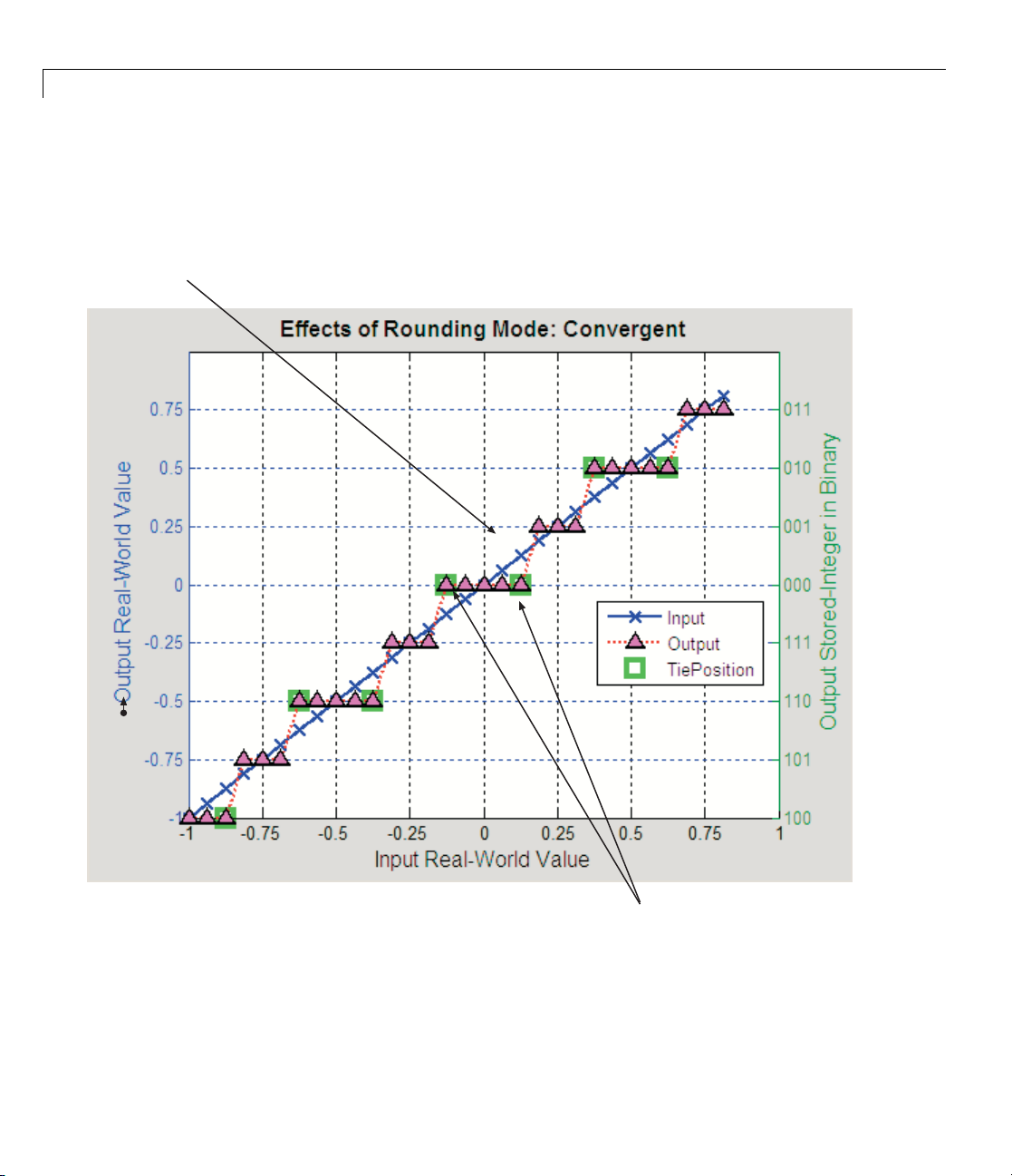
3 Arithmetic Operations

All numbers are rounded to the nearest representable number

In the MATLAB software, you can perform convergent rounding using the

convergent function. Convergent rounding is shown in the following figure.

3-8

Ties are rounded to the nearest even number

Limitations on Precision

Rounding Mode: Floor

When you round toward floor, both positive and negative numbers are rounded to negative infinity. As a result, a negative cumulative bias is introduced in the number.

In the MATLAB software, you can round to floor using the Rounding toward floor is showninthefollowingfigure.

floor function.

All numbers are rounded toward negative infinity

3-9

3 Arithmetic Operations

Rounding Mode: Nearest

When you round toward nearest, the number is rounded to the nearest representable value. In the case of a tie, representable number in the direction o f positive infinity.

In the Fixed-Point Toolbox software, you can round to nearest using the

nearest function. Rounding toward nearest is shown in the following figure.

All numbers are rounded to the nearest representable number

nearest rounds to the closest

Ties are rounded to the closest representable number in the direction of positive infinity

3-10

Limitations on Precision

Rounding Mode: Round

Round rounds to the closest representable number. In the case of a tie, it

rounds:

• Positive numbers to the closest representable number in the direction of

positive infinity.

• Negative numbers to the closest representable number in the direction

of negative infinity.

As a result:

• A small negative bias is introduced for negative samples.

• No bias is introduce d for samples with evenly distributed positive and

negative values.

• A small positive bias is introduced for positive samples.

3-11

3 Arithmetic Operations

In the MATLAB software, you can perform this type of rounding using the

round function. The rounding mode Round is shown in the following figure.

All numbers are rounded to the nearest representable number

For positive numbers, ties are rounded to the closest representable number in the direction of positive infinity

3-12

For negative numbers, ties are rounded to the closest representable number in the direction of negative infinity

Limitations on Precision

Rounding Mode: Simplest

The simplest rounding mode attempts to reduce or eliminate the need for extra rounding code in your generated code using a combination of techniques, discussed in the following sections:

• “Optimize Rounding for Casts” on page 3-13

• “Optimize Rounding for High-Level Arithmetic Operations” on page 3-14

• “Optimize Rounding for Intermediate Arithmetic Operations” on page 3-15

In nearly all cases, the simplest rounding mode produces the most efficient generated code. For a very specialized case of division that meets three specific criteria, round to floor might be more efficient. These three criteria are:

• Fixed-point/integer signed division

• Denominator is an invariant constant

• Denominator is an exact power of two

For this case, set the rounding mode to floor and the Con figuration Parameters > Hardware Implementation > Embedded Hardware > Signed integer division rounds to parameter to describe the rounding

behavior of your production target. For more in f orm ation, see “Improving Efficiency of Code That Uses Division by Constant Power of 2” in the Real-Time Workshop documentation.

Optimize Rounding for Casts. The Data Type Conversion block casts a signal with one data type to another data type. When the block casts the signal to a data type with a shorter word length than the original data type, precision is lost and rounding occurs. The simplest rounding mode automatically chooses the best rounding for these cases based on the following rules:

• When casting from one integer or fixed-point data type to another, the

simplest mode rounds toward floor.

• When casting from a floating-point data type to an integer or fixed-point

data type, the simplest mode rounds toward zero.

3-13

3 Arithmetic Operations

Optimize Rounding for High-Level Arithmetic Operations. The simplest

rounding mode chooses the best rounding for each high-level arithmetic operation. For example, consider the operation y = u

× u2/ u3implemented

using a Product block:

As stated in multiplic not specif the operan divide ope your prod

The simpl

• Rounds t

• Rounds

Config Embedd

To get t

round

to zer to zer enab mult

If th the s

e. The simplest mode rounds to zero for division for this case, but it

cod

not rely on your production target to perform the rounding, because the

can

ameter is

par

sure rounding to zero behavior.

the C standard, the most efficient rounding mode for

ation operations is always floor. However, the C standard does

y the rounding mode for division in cases where at least one of

ds is negative. Therefore, the most efficient rounding mode for a

ration with signed data types can befloororzero,dependingon

uction target.

est rounding m ode:

o floor for all nondivision operations.

to zero or floor for division, depending on the setting of the

uration Parameters > Hardware Implementation >

ed Hardware > Signed integer division rounds to parameter.

he m ost efficient code, you must set the Signed integer division

stoparameter to specify whether your production target rounds

o or to floor for integer division. Most production targets round o for integer division operations. Note that

Simplest rounding

les “mixed-mode” rounding for such cases, as it rounds to floor for iplication and to zero for division.

e Signed integer division rounds to parameter is set to

implestroundingmodemightnotbeabletoproducethemostefficient

Undefined. Therefore, you need additional rounding code to

Undefined,

3-14

Mathworks SIMULINK FIXED POINT 6 user guide

Specifications and Main Features

Frequently Asked Questions

User Manual

Getting Started

Product Overview

What You Need to Get Started

Installation

Sharing Fixed-Point Models

Demos

Physical Quantities and Measurement Scales

Introduction

Selecting a Measurement Scale

Measurement Scales: Beyond Multiplication

Example: Selecting a Measurement Scale

Why Use Fixed-Point Hardware?

Why Use the Simulink Fixed Point Software?

The Development Cycle

Simulink Fixed Point Software Features

Configuring Blocks with Fixed-Point Output

Specifying the Output Data Type and Scaling

Specifying Fixed-Point Data Types with the Data Type Assistant

Rounding

Overflow Handling

Locking the Output Data Type Setting

Real-World Values Versus Stored Integer Values

Configuring Blocks with Fixed-Point Parameters

Specifying Fixed-Point Values Directly

Specifying Fixed-Point Values Via Parameter Objects

Reading Fixed-Point Data from the Workspace

Writing Fixed-Point Data to the Workspace

Logging Fixed-Point Signals

Accessing Fixed-Point Block Data During Simulation

Fixed-Point Advisor

Fixed-Point Tool

Code Generation Capabilities

Example: Converting from Doubles to Fixed Point

About This Example

Binary-Point-Only Scaling

[Slope Bias] Scaling

Data Types and Scaling

Overview

Fixed-Point Numbers

About Fixed-Point Numbers

Signed Fixed-Point Numbers

Binary Point Interpretation

Scaling

Binary-Point-Only Scaling

Slope and Bias Scaling

Unspecified Scaling

Quantization

Example: Fixed-Point Format

Range and Precision

Range

Precision

Fixed-Point Data Type Parameters

Fixed-Point Data Type Range and Default Scaling

Range of an 8-Bit Fixed-Point Data Type — Slope and Bias Scaling

Constant Scaling for Best Precision

Scaled Doubles

What are Scaled Doubles?

When to Use Scaled Doubles

Example: Port Data Type Display

Floating-Point Numbers

About Floating-Point N umbers

Scientific Notation

The IEEE Format

The Sign Bit

The Fraction Field

The Exponent Field

Single-Precision Format

Double-Precision Format

Range and Precision

Range

Precision

Floating-Point Data Type Parameters

Exceptional Arithmetic

Denormalized Numbers

Arithmetic Operations

Overview