Mathworks SIMULINK DESIGN OPTIMIZATION 1 user guide

Download

Simulink®Design O

User’s Guide

ptimization™ 1

How to Contact The MathWorks

www.mathworks.

com

Web

comp.soft-sys.matlab Newsgroup www.mathworks.com/contact_TS.html Technical Support

suggest@mathworks.com Product enhancement suggestions

bugs@mathwo

rks.com

Bug reports

doc@mathworks.com Documentation error reports service@mathworks.com Order status, license renewals, passcodes

info@mathwo

rks.com

Sales, prici

ng, and general information

508-647-7000 (Phone)

508-647-7001 (Fax)

The MathWorks, Inc. 3 Apple Hill Drive Natick, MA 01760-2098

For contact information about worldwide offices, see the MathWorks Web site.

Simulink

The software described in this document is furnished under a license agreement. The software may be used or copied only under the terms of the license agreement. No part of this manual may be photocopied or reproduced in any form without prior written consent from The MathW orks, Inc.

FEDERAL ACQUISITION: This provision applies to all acquisitions of the Program and Documentation by, for, or through the federal government of the United States. By accepting delivery of the Program or Documentation, the government hereby agrees that this software or documentation qualifies as commercial computer software or commercial computer software documentation as such terms are used or defined in FAR 12.212, DFARS Part 227.72, and DFARS 252.227-7014. Accordingly, the terms and conditions of this Agreement and only those rights specified in this Agreement, shall pertain to and govern theuse,modification,reproduction,release,performance,display,anddisclosureoftheProgramand Documentation by the federal government (or other entity acquiring for or through the federal government) and shall supersede any conflicting contractual terms or conditions. If this License fails to meet the government’s needs or is inconsistent in any respect with federal procurement law, the government agrees to return the Program and Docu mentation, unused, to The MathWorks, Inc.

Trademarks

MATLAB and Simulink are registered trademarks of The MathWorks, Inc. See

www.mathworks.com/trademarks for a list of additional trademarks. Other product or brand

names may be trademarks or registered trademarks of their respective holders.

Patents

The MathWorks products are protected by one or more U.S. patents. Please see

www.mathworks.com/patents for more information.

Revision History

March 2009 Online only New for Version 1 (Release 2009a) September 2009 O nline only Revised for Version 1.1 (Release 2009b) March 2010 Online only Revised for Version 1.1.1 (Release 2010a)

Design Optimization™ User’s Guide

Data Analysis and Processing

Configuring a Model for Importing Data ............. 1-2

Contents

Creating an Estimation Project

ImportingDataintotheGUI

Importing Time-Domain Data into the GUI Importing Time-Series Data into the GUI Importing Complex Data into the GUI

Plotting and Analyzing Data in the GUI

Why Plot the Data Before Parameter Estimation How To Plot Data in the GUI

Preprocessing Data in the GUI

Ways to Preprocess Data Using the Data Preprocessing

Tool

.......................................... 1-14

Opening the Data Preprocessing Tool Handling Missing Data Handling Outliers Detrending Data Filtering Data Selecting Data Adding Preprocessed Data Sets to an Estimation Project Exporting Prepared Data to the MATLAB Workspace

.................................... 1-18

.................................... 1-20

............................. 1-16

................................. 1-18

.................................. 1-18

..................... 1-3

........................ 1-5

............ 1-5

.............. 1-10

................ 1-10

............. 1-11

........................ 1-11

...................... 1-14

................. 1-15

........ 1-11

.. 1-28

.... 1-31

Parameter Estimation

Overview of Parameter Estimation .................. 2-2

iii

Configuring Parameter Estimation in the GUI ....... 2-3

Creating an Estimation Task Specifying Data for Parameter Estimation Specifying Parameters to Estimate Specifying Initial States Selecting Views for Plotting Specifying Estimation Options Specifying Simulation Options Specifying Display Options

........................ 2-3

............. 2-4

................... 2-6

............................ 2-17

......................... 2-19

....................... 2-23

....................... 2-29

.......................... 2-35

Estimating Param eters in the GUI

Validating Parameters in the GUI

BasicStepsforModelValidation Loading and Importing the Validation Data Performing Validation Comparing Residuals

Accelerating Model Simulations During Estimation

About Accelerating Model Simulations During

Estimation Limitations Setting the Accelerator Mode for Parameter Estimation

Speeding Up Parameter Estimation Using Parallel

Computing

When to Use P arallel Computing for Estimating Model

Parameters How Parallel Computing Speeds Up Parameter

Estimation Specifying Model Dependencies Configuring Your System for Parallel Computing How to Use Parallel Computing in the GUI Troubleshooting

..................................... 2-50

...................................... 2-50

...................................... 2-52

.................................... 2-52

..................................... 2-53

................................... 2-62

............................. 2-43

.............................. 2-47

.................. 2-36

................... 2-40

..................... 2-40

............ 2-41

...................... 2-56

....... 2-56

............ 2-58

.. 2-50

iv Contents

Estimating Initial States

How to Estimate Initial States in the GUI Estimating Initial Conditions for Blocks with External

Initial Conditions Example — Estimating Initial States of a

Mass-Spring-Damper System

........................... 2-65

............. 2-65

............................... 2-66

..................... 2-67

Working with Estimation Projects .................. 2-78

Structure of an Estimation Project Managing Multiple Projects and Tasks Adding, Deleting and Renaming an Estimation Project Saving Control and Estimation Tools Manager Projects Loading Control and Estimation Tools Manag er Projects

................... 2-78

................ 2-79

... 2-80

.. 2-81 .. 2-82

Estimating Param e ters at the Command Line

Workflow for Estimating Parameters at the Command

Line

.......................................... 2-83

Example — Estimating Parameters and Initial States at

the Command Line Objects for Parameter Estimation How to Use Parallel Computing at the Command Line

.............................. 2-84

.................... 2-95

........ 2-83

Parameter Optimization

Overview of Optimizing Model Parameters .......... 3-2

Optimizing Parameters Using the GUI

Constraining Model Signals Specifying Design Requirements Specifying Parameters to Optimize Specifying Optimization Options Specifying the Simulation Options Plotting Responses in the Signal Constraint Window Running the Optimization

......................... 3-3

..................... 3-5

..................... 3-27

.......................... 3-39

............... 3-3

................... 3-19

.................... 3-32

... 2-116

.... 3-36

Optimizing P arameters for M odel Robustness

What Is Model Robustness? Sampling Methods for Computing Uncertain Parameter

Values How to Optimize Parameters for Model Robustness Using

the GUI Commands for Optimizing Parameters for Model

Robustness Example — Optimizing Parameters for M odel Robustness

Using the GUI

........................................ 3-43

....................................... 3-46

.................................... 3-49

.................................. 3-49

......................... 3-42

........ 3-42

Accelerating Model S imulations During

Optimization

About Accelerating Optimization Limitations Setting Accelerator Mode for Response Optimization

Speeding Up Response Optim ization Using Parallel

Computing

When to Use Parallel Computing for Response

Optimization How Parallel Computing Speeds Up Optimization Configuring Your System for Parallel Computing Specifying Model Dependencies How to Use Parallel Computing in the GUI How to Use Parallel Computing at the Command Line

.................................... 3-58

..................... 3-58

...................................... 3-58

...................................... 3-60

................................... 3-60

....... 3-61

....... 3-64

...................... 3-65

............ 3-66

.... 3-58

... 3-70

Refining and Troubleshooting Optimization Results

Troubleshooting Optimization Results

Saving and Loading Response Optimization

Projects

Saving Response Optimization Projects Saving Additional Settings Reloading Response Optimization Projects

Optimizing P arameters at the Command Line

Workflow for Optimizing Parameters a t the Command

Line Configuring a Simulink Model for Optimizing

Parameters Creating or Extracting a Response Optimization P roject Specifying Design Requirements Specifying Parameter Settings Configuring Optimization and Simulation Settings Running the Optimization

........................................ 3-82

.......................... 3-85

.......................................... 3-87

.................................... 3-88

....................... 3-93

.......................... 3-95

................ 3-72

............... 3-82

............. 3-86

........ 3-87

..................... 3-89

...... 3-94

.. 3-72

.. 3-88

vi Contents

Optimization-Based Linear Control Design

Overview of Optimization-Based Compensator

Design

Supported Time- and Frequency-Domain

Requirements

Root Locus Diagrams Open-Loop and Prefilter Bode Diagrams Open-Loop Nichols Plots Step/Impulse Response Plots

Designing Optimization-Based Controllers for LTI

Systems

How to D esign Optimization-Based Controllers for LTI

Example — Frequency-Domain Optimization for LTI

.......................................... 4-2

................................... 4-4

.............................. 4-4

............................ 4-6

........................ 4-7

........................................ 4-8

Systems

System

....................................... 4-8

........................................ 4-9

............... 4-6

Designing Linear Controllers for Simulink Models

Lookup Tables

What Are Lookup Tables? .......................... 5-2

Static Lookup Tables Adaptive Lookup Tables

Estimating Values of Looku p Tables

How to Estimate Values of a Lookup Table Example — Estimating Lookup Table Values from Data Example — Estimating Constrained Values of a Lookup

Table

Capturing Time-Varying System Behavior Using

Adaptive Lookup Tables

......................................... 5-20

............................... 5-2

............................ 5-3

................. 5-5

............. 5-5

......................... 5-37

... 4-30

.. 5-6

vii

Building Models Using Adaptive Lookup Table Blocks ... 5-37 Configuring Adaptive Lookup Table Blocks Example — Modeling an Engine Using n-D Adaptive

Lookup Table Using Adaptive L ookup Tables in Real-Time

Environment

................................... 5-44

................................... 5-60

............ 5-41

Function Reference

Parameter Estimation ............................. 6-2

Parameter Optimization

Response Optimization Projects Design Requirements Parameters Model Depende ncies Model Robustness Optimization Options Simulation Options

...................................... 6-4

.............................. 6-3

............................... 6-4

................................. 6-4

.............................. 6-4

................................ 6-4

........................... 6-3

...................... 6-3

viii Contents

Functions — Alphabetical List

Block Reference

Examples

Parameter Estimation ............................. A-2

Parameter Optimization

Optimization-Based Linear Control Design

Lookup Tables

..................................... A-2

........................... A-2

.......... A-2

Index

x Contents

Data Analysis and Processing

• “Configuring a Model for Importing Data” on page 1-2

• “Creating an Estimation Project” on page 1-3

• “Importing Data into the GUI” on page 1-5

• “Plotting and Analyzing Data in the GUI” on page 1-11

• “Preprocessing Data in the GUI” on page 1-14

1 Data Analysis and Processing

Configuring a Model for Importing Data

Before you can analyze and preprocess the estimation data, you must assign thedatatothemodel’schannels. Inordertoassignthedata,theSimulink model must contains one of the following elements:

• Top-level Inport block

Note You do not need an Inport block if your model already contains a

fixed input block, such as a Step block.

• Top-level Outport block

• Logged signal. The logged signal can be a top-level signal in the model

or a signal in the model subsystem.

For more information about the blocks and logged signals, see the Inport and O utport block reference pages and “Logging Signals” in the Simulink documentation.

In the Control and Estim ation Tools Manager GUI, the rows in the Input Data tab correspond to the model’s top-level Inport blocks. Similarly, the rows in the Output Data tab correspond to either the top-level Outport blocks or logged signals in the model.

Adding an Inport or Outport block or marking a signal for logging creates a new row in the corresponding Input Data or Output Data tab. You can use the new row to import estimation data for the corresponding signal. To view the new row, click Update Task in the Estimation Task node of the C ontrol and Estimation Tools Manager GUI.

1-2

Creating an Estimation Project

Before you begin data import, you m ust create and set up an estimation project by configuring the appropriate parameters, solvers, and cost functions. Simulink Interface (GUI) that makes setting up the estimation project quick and easy .

To create an estimation project:

1 Open the nonlinear idle speed model of an automotive engine by typing :

at the MA TLAB®prompt.

The model appears as shown next.

Design Optimization™ software provides a Graphical User

engine_idle_speed

Creating an Estimation Project

The model contains the Inport block BPAV and Outport block Engine Speed for importing input and output data, respectively. To learn more, see “Configuring a Model for Importing Data” on page 1-2.

1-3

1 Data Analysis and Processing

2 Open the Control and Estimation Tools Manager GUI by selecting Tools

> Parameter Estimation in the Simulink model window.

1-4

Control and Estimation Tools Manager GUI

The pr Estim

Note

esti

oject tree displays the project name Project - engine_idle_speed.

ation tasks are organized inside the Estimation Task node.

The Simulink model must remain open to perform parameter

mation tasks.

Importing Data into the GUI

In this section...

“Importing Time-Domain Data into the GUI” on page 1-5

“Importing Time-Series Data into the GUI” on page 1-10

“Importing Complex Data into the GUI” on page 1-10

Importing Time-Domain Data into the GUI

After you create an estimation project, as described in “Creating an Estimation Project” on page 1-3, you can import the estimation data into the GUI. To learn more about the types of data for paramete r estimation, see “Types of Data for Parameter Estimation” in the Simulink Design Optimization Getting Started Guide.

To import transient (measure d) data for your dynamic system:

Importing Data into the GUI

1 In the Control and Estimation Tools Manager, select Transient Data

under the Estimation Task node of the Workspace tree.

2 Right-click Transient Data and select New to create a New Data node.

Alternatively, you can use the New button to create this node.

1-5

1 Data Analysis and Processing

1-6

3 Select the New Data node under the Transient Data node.

The Control and Estimation Tools Manager GUI now resembles the next figure.

Importing Data into the GUI

Import Data into the Co ntrol and Estimation Tools Manager

ThetablerowsintheInput Data tab corresponds to the Inport block BPAV in the engine_idle_speed model. Similarly, the rows in the Output Data tab corresponds to the Outport block

Engine Speed.

Note The Simulink model must contain an Inport or Outport block or logged signals to enable importing data. For more information, see “Configuring a Model for Importing Data” on page 1-2.

The idle-speed model of an automotive engine contains the measured data stored in the

iodata array. The array contains two columns: the first for

input data, and the second for output data. You must import both the input and the output data, as described in the following sections:

• “Importing Input Data and Time Vector” on page 1-8

1-7

1 Data Analysis and Processing

Importing Input Data and Time Vector

To import the input data for the port BPAV:

1 In the New Data node, click the Input Data tab.

2 Right-click the Data cell and select Import to open the Data Import dialog

• “Importing Output Data and Time Vector” on page 1-9

box. Alternatively, you can use the Import button to open this dialo g box.

1-8

3 In the Data Import dialog box, select iodata from the list of variables.

Importing Data into the GUI

4 Enter 1 in the Assign the following colum ns to selected channel(s)

field, and then click Import.

5 In the Input Data tab, select the Time/Ts cell.

6 Select ti

7 Click Im port to import the time vector for the input data.

8 Click Close to close the Data Import dialog box.

Import

in the Data Import dialog box.

ingOutputDataandTimeVector

To import the output data for the port Engine Speed:

1 In the New Data node, select the Output Data tab.

2 Right

-click the Data cell and select Import to open the Data Import dialog

box.

3 In the Data Import dialog box, select iodata from the list of variables.

4 Enter 2 in the Assign the following colum ns to selected channel(s)

field to use the second column of

he Output Data tab, select the Time/Ts cell.

5 In t

iodata,andthenclickImport.

1-9

1 Data Analysis and Processing

6 Select time in the Data Import dialog box.

7 Click Im port to import the time vector for the output d ata.

8 Click Close to close the Data Import dialog box.

Importing Time-Series Data into the GUI

Time-series data is stored in time-series objects. For more information, see “Time Series Objects” in the MATLAB documentation.

When you import time-series data for parameter estimation, specify the data and time vector as t.data and t.time in the Data and Time/Ts columns of the New Data node, respectively. For more information on how to import data into the GUI, see “Importing Time-Domain Data into the GUI” on page 1-5.

Importing Complex Data into the GUI

Complex-valued data is data whose value is a complex number. For example, a signal with the value parameters of electrical systems, such as the magnitude and p hase.

1+2j is complex. You can use complex data to estimate

1-10

Note You must sample the real and imaginary parts of the data as a function ofthesametimevector.

To use complex data for parameter estimation:

1 Split the data into two data sets that contain the real and imaginary parts.

To split the data, use the MATLAB functions

2 Import both data sets into the GUI, as described in “Importing

real,andimag.

Time-Domain Data into the GUI” on page 1-5.

3 Specify both the data sets together as estimation data, as described in

“Specifying Data for Parameter Estimation” on page 2-4.

4 Estimate the parameters, as described in “Estimating Parameters in the

GUI” on page 2-36.

Plotting and Analyzing Data in the GUI

In this section...

“Why Plot the D ata Before Parameter Estimation” on page 1-11

“How To Plot Data in the GUI” on page 1-11

Why Plot the Data Before Parameter Estimation

After you import the estimation data, as described in “Importing D ata into the GUI” on page 1-5, it is useful to remove o utlie rs, smooth, detrend, or otherwise treat the data to make it more tractable for analysis and estimation purposes. To view and analyze the data characteristics, you must plot the data on a time plot.

HowToPlotDataintheGUI

To plot a data set, select the Data cell that you want to plot in the Transient Data node of the Control and Estimation Tools Manager GUI, and click Plot Data.

Plotting and Analyzing Data in the GUI

1-11

1 Data Analysis and Processing

1-12

The data is plotted on a time plot, as shown in the next figure.

Plotting and Analyzing Data in the GUI

Using the time plot, you can examine the data characteristics such as noise, outliers and portions of the data to use for estimating parameters. After you analyze the data, you the preprocess the data as described in “Preprocessing DataintheGUI”onpage1-14.

1-13

1 Data Analysis and Processing

Preprocessing Data in the GUI

In this section...

“Ways to Preprocess Data Using the Data Preprocessing Tool” on page 1-14

“Opening the Data Preprocessing Tool” on page 1-15

“Handling Missing Data” on page 1-16

“Handling Outliers” on page 1-18

“Detrending Data” on page 1-18

“Filtering Data” on page 1-18

“Selecting Data” on page 1-20

“Adding Preprocessed Data Sets to an Estimation Project” on page 1-28

“Exporting Prepared Data to the MATLAB Workspace” on page 1-31

Ways to Preprocess Data Using the Data Preprocessing Tool

After you import the estimation data, as described in “Importing D ata into theGUI”onpage1-5,youcanperformthe following preprocessing operations using the Data Preprocessing Tool in Simulink Design Optimization software:

1-14

• Exclusion — Exclude a portion of the data from the estimation process. You

can exclude data by:

- Selecting it with your mouse.

- Graphically by s electing regions on a plot.

- Using rules, such as upper or lower bounds.

• Handle missing data –– Remove missing data, or compute missing data

using interpolation.

• Handle outliers –– Remove outliers.

• Detrend — Remove mean values or a straight line trend.

• Filter — Smooth data u sing a first-order filter, an arbitrary transfer

function, or an ideal filter.

Preprocessing Data in the GUI

Opening the Data

To open the Data P

1 In the Control a

Data node under want to prepro enables the Pr

reprocessing Tool:

nd Estimation Tools Manager GUI, select the Transient

the Estimation Task node, and then choose the data you cess either in the Input Data,orOutput Data tab. This e-process button.

Preprocessing Tool

2 Click Pre-process to open the Data Preprocessing Tool.

1-15

1 Data Analysis and Processing

1-16

Tip Whe to prep Prepro

In thi used esti Impo 1-3.

Han

• “R

n you have multiple data sets, select the data set that you want

rocess from the Modify data from drop-downlistintheData

cessing Tool.

s section , the sample data set imported for preprocessing is the same as

in the

engine_idle_speed Simulink mode l. For an overview of creating

mation projects and importing data sets, see “Configuring a Model for

rting D ata” on page 1-2, and “Creating an Estimation Project” on page

dling Missing Data

emoving Missing Data” on page 1 -17

Preprocessing Data in the GUI

• “Interpolating Missing Data” on page 1-17

Removing Missing Data

Rows of missing or excluded data are represented by NaNs. To re move the rows containing missing or excluded data, select the Remove rows where check box in the MissingDataHandlingarea of the Data Preprocessing Tool GUI.

When the data set contains multiple column s of data, select all to remove rows in which all the data is excluded. Select Inthecaseofone-columndata,

any and all are equivalent.

Tip You can view the modified data in the Modified data tab of the Data Preprocessing Tool GUI.

any to remove any excluded cell.

Interpo

lating Missing Data

The interpolation operation computes the missing data values using known data values. When you select the Interpolate missing values using interpolation method check box in the Missing Data Handling area of the Data Preprocessing Tool GUI, the software interpolates the missing data values.

You can compute the missing data values using one of the following interpolation methods:

• Zero-order hold (

zoh) — Fills the missing data sample with the data value

immediately preceding it.

• Linear interpolation (

Linear) — Fills the missing data s ample with t he

average of the data values immediately p receding and f ollo wing it.

1-17

1 Data Analysis and Processing

By default, the interpolation method is set to zoh. You can select the

Linear interpolation method from the Interpolate missing values using

interpolation method drop-down list.

Tip You can view the results of interpolation in the Modified data tab of the Data Preprocessing Tool GUI.

Handling Outliers

Outliers are data values that deviate from the mean by more than three standard deviations. When estimating parameters from data containing outliers, the results may not be accurate.

To remove outliers, select the Outliers check box to activate outlier exclusion. You can set the Window length to any positiv e integer, and use confidence limits from 0 to 100%. The window length specifies the number of data points used when calculating outliers.

1-18

Removing outliers replaces the data samples containing outliers with which you can interpolate in a subse quent operation. To learn more, see “Interpolating Missing Data” on page 1-17.

NaNs,

Detrending Data

To detrend, select the Detrending check box. You can choose constant or straight line detrending. Constant detrending removes the mean of the data to create zero-mean data. Straight line detrending finds linear trends (in the least-squares sense) and then removes t hem.

Filtering Data

• “Types of Filters” on page 1-18

• “How to Filter Data” on page 1-19

Types of Filters

You have these choices for filtering your data:

Preprocessing Data in the GUI

• First order —Afilterofthetype

1τs +

whereτis the time constant that you specify in the associated fie ld .

Transfer function — A filter of the type

•

as a s a

+++

bs b s b

+++

−

…

−

where you specify the coefficients as vectors in the associated A coefficients and Bcoefficientsfields.

•

Ideal — An idealized (noncausal) filter, either stop or pass band. Specify

either filter as a two-element vector in the Range (Hz) field. These filters areidealinthesensethatthereisnofiniterollofforripple;theendsofthe ranges are perfectly horizontal in the frequency domain.

How to Filter Data

To filter the data to remove noise, select the Detrend/Filtering tab in the Data P reprocess ing Tool GUI. Select the Filtering check box, and choose the type of filter from the Select filter type drop-down list.

1-19

1 Data Analysis and Processing

Selecting Data

• “Techniques for

1-20

• “Graphically

• “Using Rules t

• “Using the Dat

Excluding Data in the Data Preprocessing Tool” on page

Selecting Data” on page 1-20

o Select Data Samples” on page 1-23

a Table to Select Data Sam ples” on p age 1-25

Techniques for Excluding Data in the Data Preprocessing Tool

You can use t excluded fr techniques

• Selecting

• Specifyi

You acco When you as red. W becomes

he data is red, and the background is gray.

rule, t

he D ata Preprocessing Tool to select a portion of the data to be

om the estimation process. You can choose one of the following

data from the Data Editing Table.

data from a plot of the data.

ng a rule.

mplish the first two manually, and for the last you specify a rule.

exclude data using manual selection, the excluded data is show n

hen you exclude data using a rule, the background color of the cell

gray. When a portion of the data is excluded both manually and by a

1-20

Note C

Editi

hanges in data are visible everywhere. When you use the Data

ng table, you can view the results in the data p lot.

Graphically Selecting Data

an exclude data graphically. Click Exclude Graphically to open the

You c

ct Points for Preprocessing Rule window.

Sele

Preprocessing Data in the GUI

The way you exclude data is similar to the way you select a region for zooming: place your cursor in the Input Data plot and drag the mouse to draw a region of exclusion.

This figure shows an example of resulting data exclusion in the input data.

1-21

1 Data Analysis and Processing

1-22

In the Output Data plot, the excluded input data produces a blank area by default. This corresponds to the youchoosetointerpolateorremovethe exclu ded da ta, the output data shows the interpolated points.

When you make changes in the Select Points for Preprocessing Rule window, they immediately appear in the Data Editing pane, and vice versa.

Selection Pane. B y default, any box that you draw with your mouse selects data for exclusion, but you can toggle between exclusion and inclusion using the Selection pane on the left side of the Select Points for Preprocessing Rule window.

NaNs that now represent excluded data. If

Preprocessing Data in the GUI

Using Rules t

A more precise way to exclude data is to use mathematical rules. The Exclusion Rules pane in the Data Preprocessing Tool allows you to enter customized rules for excluding data.

o Select Data Samples

Thesearetherulesyoucanusetoexcludedata:

• “Upper and Lower Bounds” on page 1-24

• “MATLAB Expressions” on page 1-24

1-23

1 Data Analysis and Processing

• “Flatlines” on page 1-24

Upper and Lower Bounds. Select the Bounds check box to activate upper

and lower bound exclusion. Enter numbers in the Exclude X and Exclude Y fields for upper and lower bound exclusion. By default, the exclusion rule

is to include the boundary values, but you can use the menu to exclude the boundaries as well.

MATLAB Expressions. Use the MATLAB expression field to enter any mathematical expression using MATLA B code. Use your expression for the data being tested.

Flatlines. If you have areas of your data set w h ere the data is con stan t, providing no new information, then youcanchoosetoexcludethosedata points as flatlines. The Window length field sets the minimum number of constant data points required to define the area as a flatline.

x as the variable name in

1-24

Preprocessing Data in the GUI

Example of Rule Exclusion. This figure shows data with a region of the

x-axis excluded.

Using the Data Table to Select Data Samples

The Data Editing table lists both the raw data set and the modified data that you create.

1-25

1 Data Analysis and Processing

There are data.The if you ex of numbe represe

clude rows of data in the Raw data pane, the corresponding rows

rs become red in this table. By default the Modified data pa ne

nts the rows you removed by inserting

two tabs in the Data Editing pane: Raw data and Modified

Raw Data pane shows the working copy o f the data. For example,

NaNs.

1-26

Preprocessing Data in the GUI

In the Mod complete more info

After yo

Exclude

ly or interpolate it. See “Handling Missing Data” on page 1-16 for

rmation.

u select data for exclusion, you can view it graphically by clicking

Graphically.

ified data pane, you can choose to remove the excluded data

1-27

1 Data Analysis and Processing

1-28

As you make changes in the Data Editing pane, they immediately appear in the Select Points for Preprocessing Rule window, and vice versa.

Adding Preprocessed Data Sets to an Estimation Project

After you preprocess the data using the techniques de scribed in “Ways to Preprocess Data Using the Data Preprocessing Tool” on page 1-14, you can add the da ta set to an estimatio n project either by ove r writing an existin g data set or creating a new data set.

• “Overwriting an Existing Data Set” on page 1-29

• “Creating a New Data Set” on page 1-30

Preprocessing Data in the GUI

Overwriting an Existing Data Set

To overwrite an existing data set with the preprocessed data:

1 In the Write results to area of the Data Preprocessing Tool GUI, select

the existing dataset option.

2 Choose the data set you want to overwrite from the drop-down list.

3 Click Add.

This action overwrites the selected data set with the modified data in the Control and Estimation Tools Manager GUI.

1-29

1 Data Analysis and Processing

Tip You can export the preprocessed data to the MATLAB Workspace , as

described in “Exporting Prepared Data to the MATLAB W orkspace” on page 1-31.

Creating a New Data Set

If you do not want to overwrite an existing data set with the preprocessed data, as described in “Overwriting an Existing Data Set” on page 1-29, you can create a new data set for the preprocessed data:

1 In the Write results to area of the Data Preprocessing Tool GUI, select

2 Specify the name of the data set in the adjacent field.

the new dataset option.

1-30

3 Click Add.

This action adds a new data node in the Control and Estimation Tools Manager GUI containing the modified data.

Preprocessing Data in the GUI

Tip You descri 1-31.

Expor

Afte “Add can e furt

1 In t

can export the preprocessed data to the MATLAB Workspace, as

bed in “Exporting Prepared Data to the MATLAB Workspace” on p age

ting Prepared Data to the MATLAB Workspace

r you add the preprocessed data to an estimation project, as described in

ing Preprocessed Data Sets to an Estimation Project” on page 1-28, you

xport the data set to the MATLAB Workspace. You can use the data to

her prepare it or estimate parameters using the data.

he Transient Data node of the Control and Estimation Tool s Manager

, s elect the node containing the prepared data set.

GUI

1-31

1 Data Analysis and Processing

2 Right-click the table Data cell containing the data that you want to export,

3 Specify the MATLAB variable names for the prepared data and the

4 Click OK.

and select Export.

The Export to Workspace dialog box opens.

corresponding time vector in the Data and Time fields, respectively.

The resulting MATLAB variables Workspace browser.

data and time4 appear in the MATLAB

1-32

Parameter Estimation

• “Overview of Parameter Estimation” on page 2-2

• “Configuring Parameter EstimationintheGUI”onpage2-3

• “Estimating Parameters in the GUI” on page 2-36

• “Validating Parameters in the GUI” on page 2-40

• “Accelerating Model Simulations During Estimation” on page 2-50

• “Speeding Up Parameter Estimation Using Parallel Computing” on page

2-52

• “Estimating Initial States” on page 2-65

• “Working with Estimation Projects” on page 2-78

• “Estimating Parameters at the Command Line” on page 2-83

2 Parameter Estimation

Overview of Parameter Estimation

When you estimate model parameters, Simulink Design Optim ization software compares the measured data with data generated by a Simulink model. Using optimization techniques, the software estimates the param eter and (optionally) initial conditions of states to minimize a user-selected cost function. The cost function typically calculates a least-square error between the empirical and model data signals.

After you import and preprocess the estimation data, as described in “Importing Data into the GUI” on page 1-5 and “Preprocessing Data in the GUI” on page 1-14, follow these stepstoestimatemodelparameters:

1 “Creating an Estimation Task” on page 2-3

2 “Specifying Data for Parameter Estimation” on page 2-4

3 “Specifying Parameters to Estimate” on page 2-6

4 “Specifying Initial States” on page 2 -17

2-2

5 “Selecting Views for Plotting” on page 2-19

6 “Specifying Estimation Options” on p age 2-23

7 Estimating Parameter

8 Validating Parameters

Note The Simulink model must remain open to perform parameter

estimation tasks.

To learn how to estima te parameters at the command line, see “Estimating Parameters at the Command Line” on page 2-83.

Configuring Parameter Estimation in the GUI

In this section...

“Creating an Estimation Task” on page 2-3

“Specifying Data for Parameter Estimation” on page 2-4

“Specifying Parameters to Estimate” on page 2-6

“Specifying Initial States” on page 2-17

“Selecting Views for Plotting” on page 2-19

“Specifying Estimation Options” o n page 2-23

“Specifying Simulation Options” on page 2-29

“Specifying D isplay Options” on page 2-35

Creating an Estimation Task

ThissectiondescribeshowtousetheGUItoestimateparameters. Afteryou import the transient data, as described in “Importing Data into the GUI” on page 1-5, you must create an estimation task and configure the estimation settings. To create a container that stores the estimation settings:

1 In the Control and Estimation Tools Manager, right-click the Estimation

node in the Workspace tree and select New.

2 Select the New Estimation node.

The C ontrol and Estimation Tools Manager now rese mbles the next figure.

2-3

2 Parameter Estimation

2-4

Specif

• “Prere

• “How t

ying Data for Parameter Estimation

quisite for Specifying Data” on page 2-4

oSpecifyDataintheGUI”onpage2-5

Prerequisite for Specifying Data

ecify a data set for estimation, you must have already imported the

To sp

in the GUI and created an Estimation Task, as described in “Creating

data

timation Task” on page 2-3. If your d ata contains noise or outliers,

an Es

ust also preprocess the data, as described in “Preprocessing Data in

you m

GUI” on page 1-14.

the

Configuring Parameter Estimation in the GUI

How to Specify Data in the GUI

After you select the New Estimation node, the Data Sets tab appears. Here you select the data set that you want to use in the estimation.

Select the Selected check box to the right of the New Data data set.

Note If you imported multiple data sets, you can select them for estimation by selecting the check box to the right of each desired data set. When using several data sets, you increase the estimation precisio n. However, you also increase the number of required simulations: for N parameters and M data sets, there are M*(2N+1) simulations per iteration.

Then, specify the weight of each output from this model by setting the Weight column in the Output data weights table.

2-5

2 Parameter Estimation

The relative weights are used to place more or less emphasis on specific output variables. The following are a few guidelines for specifying weights:

• Uselessweightwhenanoutputisnoisy.

• Use more weig ht when an output strongly affects parameters.

• Use more weight when it is more important to accurately match this model

output to the data.

Specifying Parameters to Estimate

• “Choosing Which Parameters to Estimate First” on page 2-6

• “How to Specify Parameters for Estimation in the GUI” on page 2-6

• “Specifying Initial Guesses and Upper/Lower Bounds” on page 2-11

• “Specifying Parameter Dependency” on page 2-13

• “Example: Specifying Independent Parameters for Estimation” on page

2-14

2-6

Choosing Which Parameters to Estimate First

Simulink Design Optimization software lets you estimate scalar, vector and matrix parameters. Estimating model parameters is an iterative process. Often, it is more practical to estimate a small g roup of parameters and use the final estima t ed values as a starting point for further estimation of parameters that are trickier. When you have a large number of parameters to estimate, select the parameters that influence the output the most to be estimated first. Making these sorts of choices involves experience, intuition, and a solid understanding of the strengths and limitations of your Simulink model.

After you estimate a subset of parameters and validate the estimated parameters, select the remaining parameters for estimation.

How to Specify Parameters for Estimation in the GUI

To select parameters for estimation:

1 In the Control and Estimation Tools Manager, select the Variables node

in the Workspace tree to open the Estimated Parameters pane.

Configuring Parameter Estimation in the GUI

2 In the Estimated Parameters pane, click Add to open the S e lect

Parameters dialog box.

2-7

2 Parameter Estimation

The dialog box lists all the variables in the model workspace and the MATLAB workspace that the model uses. You can use the mouse to select theparameterstoestimate.

2-8

You can also enter parameters, separated by commas, in the Specify expression field of the Select Parameters dialog box. The parameters

can be stored in one of the following:

• Simulink software parameter object

Example: For a Simulink parameter object

• Structure

Example: For a structure S, type S.fieldname (where fieldname represents the name of the field that contains the parameter).

• Cell array

Example: Type

• MATLAB array

Example: Type

C{1} to select the first element of the C cell array.

a(1:2) to select the first column ofa2-by-2arraycalled

k,typek.value.

Configuring Parameter Estimation in the GUI

Sometimes, models have parameters that are not explicitly defined in the model itself. For example, a gain workspace as

k=a+b,wherea and b are not defined in the model but k

k could be defined in the MATLAB

is used. To add these independent parameters to the Select Parameters dialog box, see “Specifying Parameter Dependency” on page 2-13.

3 Select the last seven parameters: freq1, freq2, freq3, gain1, gain2,

gain3,andmean_speed,andthenclickOK.

Note You need not estimate the parameters selected here all at once. You can first select all the parameters that you are interested in, and then later selecttheonestoestimateasdescribedinthenextstep.

The C ontrol and Estimation Tools Manager now rese mbles the next figure.

2-9

2 Parameter Estimation

To learn how to specify the settings in the Default settings area of the pane, see “Specifying Initial Guesses and Upper/Lower Bounds” on page 2-11.

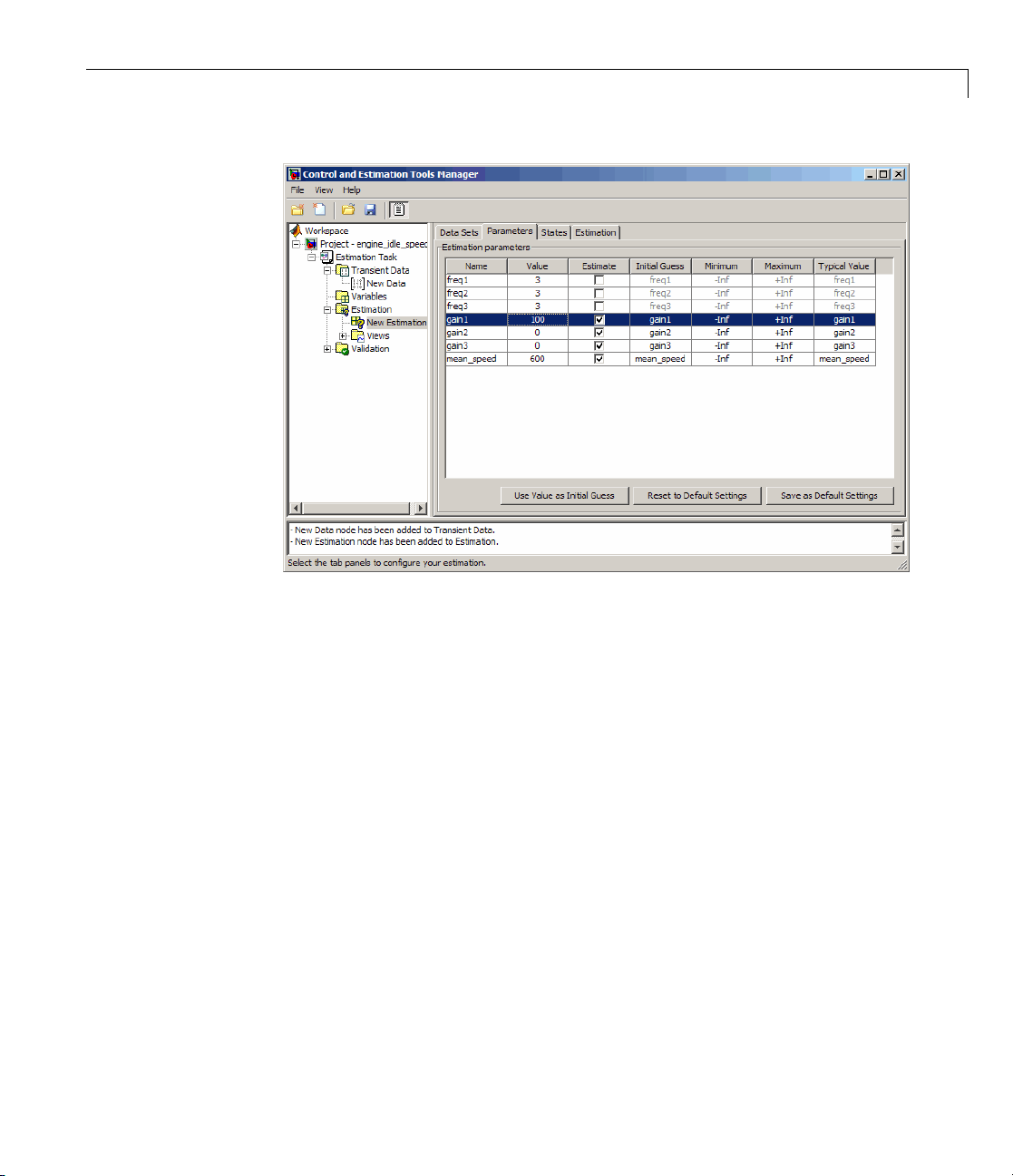
4 In the New Estimation node of the Control and Estimation Tools

Manager GUI, select the Parameters tab . In this pane, you select which parameters to estimate and the range of values for the estimation.

a Select the parameters you want to estimate by selecting the check box

in the Estimate column.

b EnterinitialvaluesforyourparametersintheInitial Guess column.

The default values in the Minimum and Maximum columns are

-Inf

and +Inf, respectively, but you can select any range you want. For more information, see “Specifying Initial Guesses and Upper/Lower Bounds” on page 2-11.

Note When you specify the Minimum and Maximum values for the parameters here, it d oes not affect your settings in the Variables node. Youmakethesechoicesonaperestimationbasis. Youcanmovedatato and from the Variables node into the Estimation node.

For this example, select gain1, gain2, gain3 and mean_speed for estimation and set

gain1 to 10, gain2 to 100, gain3 to 50, and mean_speed

to 500. Alternat ively, use any initial values you like.

If you have good reason to believe a parameter lies within a finite range, it is usually best not to use the default minimum and maximum values. Often, there are computational advantages in specifying finite bounds if you can. It can be very important to specify lower and upper bounds. For example, if a parameter specifies the weight of a part, be sure to specify

as the absolute lower bound if better knowledge is unavailable.

The C ontrol and Estimation Tools Manager now rese mbles the next figure.

2-10

Configuring Parameter Estimation in the GUI

Specifying Initial Guesses and Upper/Lower Bounds

After you select parameters for estimation in the Variables node of the Control and Estimation Tools Manager GUI, the Estimated Parameters tab in the Control and Estimation Tools Manager looks like the following figure.

2-11

2 Parameter Estimation

2-12

For eac

• Initia

• Minimu

• Maxim

• Typic

hparameter,usetheDefault settings pane to specify the following:

lguess— The value the estimation uses to start the process.

al value — The average order of magnitude. If you exp ect your

meter to vary over several orders of magnitude, enter the number

para

specified the average o rder of magnitude you expect. For example, if

that

initial guess is 10, but you expect the parameter to vary between

your

d 1000, enter 100 (the average of the order of magnitudes) for the

10 an

ical value.

typ

m — The smallest allowable parameter value. The default is

um — The largest allowable parameter value. The default is

-Inf.

+Inf.

Configuring Parameter Estimation in the GUI

You use the typical value in two ways:

• To scale paramete rs with radically different orders of magnitude for equal

emphasis during the estimation. For example, try to select the typical values so that

anticipated value

typical value

≅ 1

initial value

typical value

≅ 1

• To put more of less emphasis on specific parameters. Use a larger typical

value to put more emphasis on a parameter during estimation.

Specifying Parameter Dependency

Sometimes parameters in your model depend on independent parameters that do not appear in the model. The following steps give an overview of how to specify independent parameters for estimation:

1 Add the independent parameters to the model workspace (along with

initial values).

2 Define a Simulation Start function that runs before each simulation of the

model. This Simulation Start function defines the relationship between the dependent parameters in the model and the independent parameters in the model workspace.

3 The independent parameters now appear in the Select Parameters dialog

box. Add these parameters to the list of parameters to be estimated.

Caution Avoid adding independent parameters together with their corresponding dependent parameters to the lists of parameters to be estimated. Otherwise the estimation could give incorrect results. For example, when a parameter

x depends on the parameters a and b,avoid

adding all three parameters to the list.

2-13

2 Parameter Estimation

For an example of how to specify independent parameters, see “Example: Specifying Independent Parameters for Estimation” on page 2-14.

Example: Specifying Independent Parameters for Estimation

Assume that the parameter Kint in the model srotut1 is related to the parameters the i nitial values of instead of Kint, first define these parameters in the model workspace. To do this:

1 At the MATLAB prompt, type

srotut1

This opens the srotut1 model window.

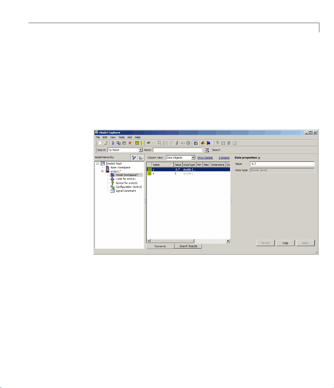
2 Select View > Model Explorer from the srotut1 w i ndow to open the

Model Explorer window.

x and y according to the relationship Kint=x+y. Also assume that

x and y are 1 and -0.7 respectively. To estimate x and y

2-14

3 In the Model Hierarchy tree, select srotut1 > Model Workspace.

Configuring Parameter Estimation in the GUI

4 Select Add > MATLAB Variable to add a new variable to the model

workspace. A new variable with a default name

Var appears in the Name

column.

5 Double-click Var to make it editable and change the variable name to x.

Edit the initial Value to

6 Repeat steps 4 and 5 to add a variable y with an initial value of -0.7.

The Model Explorer window resembles the following figure.

7 To add

Kint a

Prop

8 In the Model Properties window , click the Callbacks tab.

9 To enter a Simulation start function, select StartFcn*, and type the name

of a new function. For example,

the Sim ulation Start function that defines the relationship between

nd the independent parameters

erties in the

srotut1 model window.

srotut1_start in the Simulation start

x and y, select File > Model

function panel. Then, click OK.

2-15

2 Parameter Estimation

10 Create a MATLAB file named srotut1_start. The content of the file

defines the relationship between the parameters in the model and the parameters in the workspace. For this example, the content resembles the following:

wks = get_param(gcs, 'ModelWorkspace') x = wks.evalin('x') y = wks.evalin('y') Kint = x+y;

Note You m ust first use the get_param function to get the variables x and

y from the model workspace before you can use them to define Kint.

When you select parameters for estimation in the Variables node of Control and Estimation Tools Manager,

x and y appear in the Select Parameters

dialog box.

2-16

Configuring Parameter Estimation in the GUI

Specifying Initial States

• “When to Specify Initial States Versus Estimate Initial States” on page 2-17

• “How to Specify Initial States in the GUI” on page 2-17

When to Specify Initial States Versus Estimate Initial States

Often, sets of measured data are collected at various times and under different initial conditions. When you estimate model parameters using one data set and subsequently run another estimation with a second data set, your parameter v alues may not match. Given that the Simulink Design Optimization software attempts to find constant values for parameters, this is clearly a problem.

You can estimate the initial conditions using procedures that are similar to thoseyouusetoestimateparameters. Youcanthenusetheseinitialcondition estimates as a basis for estimating parameters for your Simulink model. The Control and Estimation Tools Manager has an Estimated States pane that lists the states available for initial condition estimation. To learn how to estimate initial states, see “Estimating Initial States” on page 2-65.

How to Specify Initial States in the GUI

After you select parameters for estimation, as described in “Specifying Parameters to Estimate” on page 2-6, you can s pecify initial conditions of states in your model. By default, the estimation uses initial conditions specified in the S i mulink model. If you want to specify initial cond iti ons other than the defaults, use the State Data tab. You can select the State

Data tab in the New Data node under the Transient Data node in the Workspace tree.

2-17

2 Parameter Estimation

2-18

Configuring Parameter Estimation in the GUI

To specify t he initial condition of a state for the engine_idle_speed model:

1 Select the Data cell associated with the state.

2 Enter the initial conditions. In this example, enter -0.2 for State - 1 of

the engine_idle_speed/Transfer Fcn.ForState - 2,enter

cting Views for Plotting

Sele

• “Typ

• “Ba

es of Plots” on page 2-19

sicStepsforCreatingPlots”onpage2-20

Types of Plots

u can choose the plot type from the Plot Type drop-down list. The following

pes of pl o ts are available for viewing and evaluating the estimation:

2-19

2 Parameter Estimation

• Cost function — Plot the cost function values.

Measured and simulated — Plot empirical data against simulated data.

•

Parameter sensitivity — Plot the rate of change of the cost function as a

•

function of the change in the parameter. That is, plot the derivative of the cost function with respect to the parameter being varied.

•

Parameter trajectory — Plot the parameter values as they change.

Residuals — Plot the error betw een the experimental data and the

•

simulated output.

Basic Steps for Creating Plots

Before you begin estimating the parameters, you must create the plots for viewing the progress of the estimation.

Note An estimation must be created before creating views. Otherwise, the Options tablewillbeempty.Tolearnmore,see“CreatinganEstimation Task” on page 2-3.

2-20

To create plots for viewing the estimation progress, follow the steps below:

1 Right-click the Views node in the Control and Estimation Tools Manager

and select New.

Configuring Parameter Estimation in the GUI

2 In the Workspace tree, select New View to open the View Setup pane.

2-21

2 Parameter Estimation

3 In the Select plot types table, select the Plot Type from the drop-down

list. In this e xample , select

Cost function.

2-22

4 Selec

will b

5 In the Options area, select the check-box for both Plot 1 and Plot 2.

6 Click Show Plots. This displays an empty cost function plot and a plot of

Measured and simulated as the Plot Type for Plot 2.Thisplot

e used in validating estimated parameters.

the measured data.

Configuring Parameter Estimation in the GUI

When you perform the estimation, the plot updates automatically.

Specifying Estimation Options

• “Accessing Estimation Options” on page 2-24

• “Supported Estimation Methods” on page 2-25

• “Selecting Optimization Termination Options” on page 2-27

• “Selecting Additional Optimization Options” on page 2-27

• “Specifying Goodness of Fit Criteria (Cost Function)” on page 2-28

• “How to Specify Estimation Op t ions in the GUI” on page 2-28

2-23

2 Parameter Estimation

Accessing Estimation Options

In the New Estimation node in the Workspace tree, click the Estimation tab.

2-24

Click Estimation Options. This action opens the Options- New Estimation dialog box where you can specify the estimation method, algorithm options and cost function for the estimation.

Configuring Parameter Estimation in the GUI

The following sections describe the estimation method settings and cost function:

• “Supported Estimation Methods” on page 2-25

• “Selecting Optimization Termination Options” on page 2-27

• “Selecting Additional Optimization Options” on page 2-27

• “Specifying Goodness of Fit Criteria (Cost Function)” on page 2-28

Supported Estimation Methods

Both the Method and Algorithm options define the optimization method. Use the Optimization method area of the Options dialog box to set the estimation method and its algorithm.

For the Method option, the four choices are:

•

Nonlinear least squares (default) — Uses the Optimization Toolbox™

nonlinear least squares function

Gradient descent — Uses the Optimization T oolbo x function fmin con.

•

lsqnonlin.

2-25

2 Parameter Estimation

• Pattern search — Uses the pattern search method patternsearch.This

option requires Global Optimization Toolbox software.

•

Simplex search — Uses the Optimization Toolbox function fminsearch,

which is a direct search method. problems and is sometimes faster than

Simplex search is most useful for simple

fmincon for models that contain

discontinuities.

The following table summarizes the Algorithm options for the

least squares

Method Algorithm Option

Nonlinear least squares

and G radi ent descent estimation methods:

Learn More

• Trust-Region-Reflective

(default)

Levenberg-Marquardt

•

In the Optimization Toolbox documentation, see:

• “Large Scale

Trust-Region Reflective Least Squares”

• “Levenberg-Marquardt

Method”

Gradient descent

• Active-Set (default)

Interior-Point

•

• Trust-Region-Reflective

In the Optimization Toolbox documentation, see:

• “fmincon Active

Set Algorithm”

• “fmincon Interior

Point Algorithm”

Nonlinear

2-26

• “fmincon Trust

Region Reflective Algorithm”

Configuring Parameter Estimation in the GUI

Selecting Optimization Termination Options

Specify termination options in the Optimization options area.

Several options define when the optimiz ation terminates:

• Diff max change — The maximum allowable change in variables

for finite-difference derivatives. See Toolboxdocumentation for details.

• Diff min change — The minimum allowable change in variables for

finite-difference derivatives. See documentation for details.

• Parameter tolerance — Optimization terminates when successive

parameter values change by less than this number.

fmincon in the Optimization

fmincon in the Optimization Toolbox

• Maximum fun evals — The maximum number of cost function

evaluations allowed. The optimization terminates when the number of function evaluations exceeds this value.

• Maximum iterations — The maximum number of iterations allowed. The

optimization terminates when the number of iterations exceeds this value.

• Function tolerance — The optimization terminates when successive

function values are less than this value.

By varying these parameters, you can force the optimization to continue searching for a solution or to continue searching for a more accurate solution.

Selecting Additional Optimization Options

At the bottom of the Optimization options pane is a group of additional optimization options.

2-27

2 Parameter Estimation

Additional options for optimization include:

• Display level — Specifies the form of the output that appears in the

MATLAB command window. The options are information after each iteration,

None, which turns off all output, Notify,

which displays output only if the function does not converge, and

Iteration,whichdisplays

Final,

which only displays the final output. Refer to the Optimization Toolbox documentation for more information on w hat type of iterative output each method displays.

• Gradient type — When using

squares

difference methods. The

as the Method, the gradients are calculated based on finite

Refined method offers a more robust and less

noisy gradient calculation method than to run optimizations using the

Gradient Descent or Nonlinear least

Basic,althoughitdoestakelonger

Refined method.

Specifying Goodness of Fit Criteria (Cost Function)

The cost function is a function that estimation methods attempt to minimize. You can specify the cost function at the bottom of the Optimization options area.

You hav

• Cost fu

• Use ro

e the following options when selecting a cost function:

nction —Thedefaultis

-squares approach. You can also use

least

SSE (sum of squared errors), which uses a

SAE, the sum of absolute errors.

bust cost — Makes the optimizer use a robust cost function instead

default least-squares cost. This is useful if the experimental data has

of the

outliers, or if your data is noisy.

many

How to Specify Estimation Options in the GUI

can set several options to tune the results of the estimation. These

You

ions include the optimization methods and their tolerances.

opt

2-28

et options f or estimation:

To s

lect the New Estimation node in the Workspace tree.

1 Se

Configuring Parameter Estimation in the GUI

2 Click the Estimation tab.

3 Click Estimation Options to open the Options dialog box.

4 Click the Optimization Options tab and specify the options.

Specifying Simulation Options

• “Accessing Simulation Options” on page 2-29

• “Selecting Simulation Time” on page 2-30

• “Selecting Solvers” on page 2-32

Accessing Simulation Options

To estimate paramete rs of a model, Simulink Design Optimization software runs simulations of the model.

To set options for simulation:

1 Select the New Estimation node in the Workspace tree.

2 Click the Estimation tab.

3 Click Estimation Options to open the Options dialog box.

2-29

2 Parameter Estimation

4 Click the Simulation Options tab and specify the options, as described in

the following sections:

2-30

• “Selecting Simulation Time” on page 2-30

• “Selecting Solvers” on page 2-32

Selecti

You can specify the simulation start and stop times in the Simulation time area of the Simulation Options tab.

By default, Start time and Stop time are automatically computed based on thestartandstoptimesspecifiedintheSimulinkmodel.

To set alternative start and stop times for the optimization, enter the new times under Simulation time. This action overwrites the sim ulation start andstoptimesspecifiedintheSimulinkmodel.

ng Simulation Time

Configuring Parameter Estimation in the GUI

Simulation Time for Data Sets with Different Time Lengths. Simulink Design Optimization software can simulate models containing empirical data sets of different time lengths. You can use experimental data sets for estimation that contain I/O samples collected at different time points.

The following example shows a single-input, tw o-output model for which you want to estimate the parameters.

y1(t)

u(t)

y2(t)

The model uses two output data sets containing transient data samples for parameter estimation:

• Output y1(t) at time points

• Output y2(t) at time points

The simulation time t is computed as:

tt t tttt tt

=∪=

This new set ranges from tmin to tmax.Thevaluestmin and tmax represent the minimum and maximum time points in t respectively.

When you run the estimation, the model is simu la ted over the time range t. Simulink extracts the simulat ed data for eac h output based on the following criteria:

• Start time — Typically, the start time in the Simulink model is set to

For a nonzero start time, the simulated data corresponding to time points

before

,,,,.....,

{}

1112212

for y1(t) and

tttt

ttt t

212

for y2(t) are discarded.

, ,....

{}

112

, ,.....

{}

122

2-31

2 Parameter Estimation

• Stop time —Ifthestoptime

stop≥max

,thesimulateddata corresponding to time points in t1 are extracted for y1(t). Similarly, the simulated data for time points in t2 are extracted for y2(t).

If the stop time

stop<max

, the data spanning time points

> t

stop

are

discarded for both y1(t) and y2(t).

Selecting Solvers

When running the estimation, the software solves the dynamic system using one of several Simulink solvers.

Specify the solver type and its options in the Solver options area of the Simulation Options tab of the Options dialog box.

The solver can be one of the following Type:

•

Auto (default) — Uses the simulation settings specified in the Simulink

model.

•

Variable-step — Variable-step solvers keep the error within specified

tolerances by adjusting the step size the solver uses. For example, if the states o f your model are likely to vary rapidly, you can use a variable-step solverforfastersimulation. Formore information on the variable-step solver options, see “Variable-Step Solver Options” on page 2-33.

2-32

•

Fixed-step — Fixed-step solvers use a constant step-size. For more

information on the fixed-step solver options, see “ Fix ed-Step Solver Options” on page 2-34.

See “Choosing a Solver” in the Simulink documentation for information about solvers.

Configuring Parameter Estimation in the GUI

Note To obtain faster simulations during estimation, you can change the solver Type to

Variable-step or Fixed-step. Howev er, the estimated

parameter values apply only for the chosen solver type, and may differ from valuesyouobtainusingsettingsspecified in the Simulink model.

Variable-Step Solver Options . When you select Variabl e-st ep as the solver Type, you can choose one of the following as the Solver:

•

Discrete (no continuous states)

• ode45 (Dormand-Prince)

• ode23 (Bogacki-Shampine)

• ode113 (Adams)

• ode15s (stiff/NDF)

• ode23s (stiff/Mod. Rosenbrock)

• ode23t (Mod. s tiff/Trapezoidal)

• ode23tb (stiff/TR-BDF2)

You can also specify the following parameters that affect the step-size of the simulation:

• Maximum step size — The largest step-size the solver can use during a

simulation.

• Minimum step size — The smallest step-size the solver can use during a

simulation.

• Initial step size — The step-size the solver uses to begin the simulation.

2-33

2 Parameter Estimation

• Relative tolerance — The largest allowable relative error at any step in

the simulation.

• Absolute tolerance — The largest allowable absolute e rror at any step in

the simulation.

• Zero crossing control —Setto

the signal crosses the x-axis. This option is useful when using functions that are nonsmooth and the output depends on when a signal crosses the x-axis, such as absolute values.

By default, the software automatically chooses the values for these options. To specify your own values, enter them in the appropriate fields. For more information, see “Solver Pane” in the Simulink documentation.

Fixed-Step Solver Options. When you select Type, you can choose one of the following as the Solver:

•

Discrete (no continuous states)

• ode5 (Dormand-Prince)

• ode4 (Runge-Kutta)

• ode3 (Bogacki-Shanpine)

• ode2 (Heun)

• ode1 (Euler)

on for the solver to compute exactly where

Fixed-step as the solver

2-34

You can also specify the Fixed step size value, which determines the step size the solver uses during the simulation. By default, the software automatically chooses a value for this option. For more information, see “Fixed-step size (fundamental sample time)” in the Simulink documentation.

Configuring Parameter Estimation in the GUI

Specifying Display Options

You can specify the display options by clicking Display Options in the Estimation tab in the Control and E stimation toolsManager. Thisopensthe

following dialog box.

Clearing a check box implies that feature will not appear in the display table as the estimation progresses. To learn more about the display table, see “Displaying Iterative Output” in the Optimization Toolbox documentation.

2-35

2 Parameter Estimation

Estimating Parameters in the GUI

Before you begin estimating the parameters, you must have configured the estimation data and parameters, and specified estimation and simulation options, as described in “Configuring Parameter Estimation in the GUI” on page 2-3.

To start the estimation, select the New Estimation node in the Control and Estimation Tools Manager and select the Estimation tab.

Click Start to begin the estimation process. At the end of the iterations, the window should resemble the following:

2-36

Usually, a lower cost function value indicates a successful estimation, meaning that the experimental data matches the model simulation with the estimated parameters.

Estimating Parameters in the GUI

Note For information on types of problems you may encounter using optimization solvers, see “Steps to Take After Running a Solve r” in the Optimization Toolbox documentation.

The Estimation pane displays each iteration of the optimization methods. To see the final values for the parameters, click the Parameters tab.

ThevaluesoftheseparametersarealsoupdatedintheMATLABworkspace. IfyouspecifythevariablenameintheInitial Guess column, you can restart the e stim a tion from where you left off at the end of a previous estimation.

After the estimation process completes, the cost function minimization plot appearsasshowninthefollowingfigure.

2-37

2 Parameter Estimation

2-38

If the optimization went well, you should see your cost function converge on a minimum value. The lower the cost, the more successful is the estimation.

You can also examine the measured versus simulated data plot to see how closely the simulated data matches the measured estimation data. The n ext figure shows the measured versus simulated data plot generated by running the estimation of the

engine_idle_speed model.

Estimating Parameters in the GUI

2-39

2 Parameter Estimation

Validating Parameters in the GUI

In this section...

“Basic Steps for Model Validation” on page 2-40

“Loading and Importing the Validation Data” on page 2-41

“Performing Validation” on page 2-43

“Comparing Residuals” on page 2-47

Basic Steps for Model Validation

After you complete estimating the parameters, as described in “Estimating Parameters in the G UI” on page 2-36, you must validate the results against another set of data.

The steps to validate a model using the Control and Estimation Tools Manager are:

2-40

1 Import the validation data set to the Transient Data node.

2 Add a new validation task in the Validation node in the Workspace tree.

3 Config

4 Click Show Plots in the Validation Setup pane and view the results

5 Compare the validation plots to the corresponding view plots to see if they

The basic difference between the validation and views features is that you can run validation after the estimation is complete. All views should be set up before an estimation, and you can watch the views update in real time. Validations can use other validation data sets for comparison with the model response. Also, validations appear after you hav e completed an e stimatio n and do not update.

ure the validation settings by selecting the plot types and the

ation data set from the Validation Setup pane.

valid

in the plot window.

match.

Validating Parameters in the GUI

You can validate your data by comparing measured vs. simulated data for your estimation data and validation data sets. Also, it is often useful to compare residuals in the same way.

Loading and Importing the Validation Data

To validate the estimated parameters computed in “Estimating Parameters in the GUI” on page 2-36, you must first import the data into the Control and Estimation Tools Manager GUI.

To load the validation data, type

load iodataval

at the MATLAB prompt. This loads the data into the MATLAB workspace. The next step is to import this data into the Control and Estimation Tools Manager. See “Importing Data into the GUI” on page 1-5 for information on importing d ata, but the quickest way is to follow these steps:

1 Right-click the Transient Data node in the Workspace tree in the

Control and Estimation Tools Manager and select New.

2 Select New Data (2) from the Transient Data pane.

3 Right-click the New Data (2) node in the Workspace tree and s ele ct

Rename. Change the name of the data to Validation Data.

4 In the Input Data pane, select the Data cell associated with Channel

and click Import. In the Data Import dialog box, select iodataval

-1

and assign column 1 to the selected channel by entering 1 in the Assign columns field. Click Import to import the input data.

2-41

2 Parameter Estimation

5 Select the Time/Ts cell and import time using the Data Import dialog box.

6 Similarly, in the Output Data pane, select Time/Ts and import time.

2-42

7 In the Out

and cli

-1

put Data pane, select the Data cell associated with ck Import. Import the second column of data in

iodataval by

Channel

Validating Parameters in the GUI

selecting it from the list in the Import Data dialog box and entering 2 in the Assign columns field. Click Import to import the output data.

The Control and Estim ation Tools Manager should resemble the next figure.

Perfo

Afte the V New. Too

rming Validation

r you import the validation data, as described in “Loading and Importing

alidation Data” on page 2-41, right-click the Validation node and select

This creates a New Validation node in the Control and Estimation

ls Manager.

2-43

2 Parameter Estimation

2-44

To perf

1 Select

Valida

orm the validation:

the New Validation no de in the Workspace tree to open the

tion Setup pane.

Validating Parameters in the GUI

2 Click the Plot Type cell for Plot 1 and select Measured and si mula ted

from the d rop-down menu.

3 In the Options area, select Va lid ation Data in the Validation data set

drop-down list.

4 Click Show Plots to open a plot figure window as shown next.

2-45

2 Parameter Estimation

2-46

Measured Versus Simulated Data Plot for Validation Data

5 Compare

the val “Selec

idation data. For more information on how to create this plot, see

ting Views for Plotting” on page 2-19.

this plot with the plot of

Measured and simulated data for

Validating Parameters in the GUI

Measured and Simulated Data Views Plot

Comparing Residuals

To look at the residuals, select Resid uals as the Plot Type for Plot 2 in the New Validation pane. In the Options area, select the Plot 2 check box and click Show Plots. The following figure shows the resulting residuals plot.

2-47

2 Parameter Estimation

2-48

Plot of Residuals Using the Validation Data

Compare the validation data residuals with the original data set residuals from the Views node in the Workspace tree. T o create the plot of residuals for the orig inal data set, select the New View node and choose the Plot Type.

Residuals as

Validating Parameters in the GUI

Plot of Residuals Using the Test Data

The plot on the left agrees with the plot of the residuals for the validation data. The right side has no plot because residuals were not calculated for the validation data during the original estimation process.

2-49

2 Parameter Estimation

Accelerating Model Simulations During Estimation

In this section...

“About Accelerating Model Simulations During Estimation” on page 2-50

“Limitations” on p age 2-50

“Setting the Accelerator Mode for Parameter Estimation” on page 2-50

About Accelerating Model Simulations During Estimation

You can accelerate the parameter estimation computations by changing the simulation mode of your Simulink model. Simulink Design Optimization software supports information about these modes, see “Accelerating Models” in the Simulink documentation.

Normal and Accelerator simulation modes. For more

The default simulation mode is interpreted code, rather than compiled C code during simulations.

In the simulations during estimation with compiled C code. Using compiled C code speeds up the simulations and reduces the time to estimate parameters.

Accelerator mode, Simulink Design Optimization software runs

Normal. In this mode, Simulink software uses

Limitations

You cannot use the Accelerator mode if your model co ntains a lgebraic loops. If the model contains MATLAB function blocks, you must either remove them or replace them with Fcn blocks.

Setting the Accelerator Mode for Parameter Estimation

To set the simulation mode to Accelerator, open the Simulink model window and perform one of the following actions:

• Select Simulation > Accelerator.

• Choose

Accelerator from the drop-down list as shown in the next figure.

2-50

Accelerating Model Simulations During Estimation

Tip To obtain the maximum performance from the Accelerator mode, close all Scope blocks in your model.

2-51

2 Parameter Estimation

Speeding Up Parameter Estimation Using Parallel Computing

In this section...

“When to Use Parallel Computing for Estimating Model Parameters” on page 2-52

“How Parallel Computing Speeds Up Parameter Estimation” on page 2-53

“Specifying Model Depende ncies” on page 2-56

“Configuring Your System for Parallel Computing” on page 2-56

“How to Use Parallel Computing in the GUI” on page 2-58

“Troubleshooting” on page 2-62

When to U Model Pa

You can u Toolbo Using p cases:

• The mo

• The

• The m

Whe dis MAT th si on Es

x™ software to speed up parameter estimation of Simulink models.

arallel computing may reduce the estimation time in the following

near least squares

Nonli

ation method.

estim

attern search

odel is complex and takes a long time to simulate.

n you use parallel computing, Simulink Design Optimization software

tributes independent simulations to run them in parallel on multiple

LAB sessions, also known as workers. The time required to simulate

e model dominates the total estimation time. Therefore, distributing the

mulations significantly reduces the estimation time. For more information

the expected speedup, see “How Parallel Computing Speeds Up Parameter

timation” on p age 2-53.

se Parallel Computing for Estimating

rameters

se Simulink Design Optimization software with Parallel Computing

del contains a large number parameters to estimate, and the

or Gradient descent is selected as the

method is selected as the estimation method.

2-52

Speeding Up Parameter Estimation Using Parallel Computing

The following sections describe how to configure your system, and use parallel computing:

• “Configuring Your System for Parallel Compu ting ” on page 2-56

• “How to Use Parallel Computing in the GUI” on page 2-58

• “How to Use Parallel Computing at the Command Line” on page 2 -116

How Parallel Computing Speeds Up Parameter Estimation

You can enable parallel computing with the Nonlinear l east squares,

Gradient descent and Pattern search estimation methods in the Simulink

Design Optimization software. The following sections describe how parallel computing speeds up the estimation:

• “Parallel Computing with Nonlinear least squares and Gradient descent

Methods” on page 2-53

• “Parallel Computing with the Pattern search Method” on page 2-54

Parallel Computing with Nonlinear least squares and Gradient descent Methods

When you select Gradient descent as the estimation method, the model is simulated during the following computations:

• Objective value computation — One simulation per iteration

• Objective gradient computations — Two simulations for every tuned

parameter per iteration

• Line search computations — Multiple simulations per iteration

The total time, given by the following equation:

TTNTNTT NNtotal p ls p ls=+ × + × =×+××+())()(( )()212

whereTisthetimetakentosimulatethemodelandisassumedtobeequal

for all simulations, the number of line searches.

, taken per iteration to perform these simulations is

Ttotal

is the number of parameters to estimate, and

Nls

2-53

2 Parameter Estimation

When you use parallel computing, Simulink Design Optimization software distributes the simulations required for objective gradient computations. The simulation time taken per iteration when the gradient computations

are performed in parallel,

TtotalP

, is approximately given by the following

equation:

totalP

T T ceil

where

⎛

⎞

()()(212

⎜

⎝

T N T T ceil

×× + × = × +×

⎟ ⎠

is the number of MATLAB workers.

⎛

⎞

ls)

+ N

⎜

⎟

⎝

⎠⎠

Note The equation does not include the tim e overheads associated with configuring the system for parallel computing and loading Simulink software on the rem ote MATLAB workers.

The expected reduction of the total estim ation time is given by the following equation:

⎛

ceil

+×

totalP

total

12(

+×

For example, for a model with N

the total estimation time equals

⎞

⎜

⎟

⎝

⎠

)

pls

=3, Nw=4,andNls=3, the expected reduction of

⎛

+×

ceil

1233

+×+

()

⎞

⎜

⎟

⎝

⎠

2-54

Parallel Computing with the Pattern search Method

The Pattern search method uses search and poll sets to create and compute a set of candidate solutions at each estimation iteration.

Speeding Up Parameter Estimation Using Parallel Computing

The total time,

, taken per iteration to perform these simulations, is

Ttotal

given by the following equation:

TTNNTNNTNNNtotal p ss p ps p ss ps=× × +×× =× × +(( ()))

whereTisthetimetakentosimulatethemodelandisassumedtobeequal

for all simulations,

is the number of parameters to estimate,

factor for the search set size, and

is a factor for the p oll set size .

Nps

Nss

is a

When you use parallel computing, Simulink Design Optimization software distributes the simulations required for the search and poll set computations, which are evaluated in separate parfor loops. The simulation time taken pe r

iteration when the search and poll sets are computed in parallel,

TtotalP

is given by the following equation:

T T ceil N

totalP p

=× × +× ×

(( ))(( ))

T ceil N

=× ×

where

is the number of MATLAB workers.

((

N N

T ceil N

sss

ceil N

)( ))+×

Note The equation does not include the tim e overheads associated with configuring the system for parallel computing and loading Simulink software on the rem ote MATLAB workers.

The expected speed up for the total estimation time is given by the following equation:

totalP

total

ceil N

×+ ×

()( )

NN N

pssps

ceil N

()

For example, for a model with N

×+ ×

ceil ceil()()

speedup equals

×+

3152

()

=3, Nw=4, Nss=15,andNps=2,theexpected

027

2-55

2 Parameter Estimation

Using the Pattern search method with parallel computing may not speed up the estimation time. When you do not use parallel computing, the method stops searching for a candidate solution at each iteration as soon as it finds a solution better than the current solution. When you use parallel computing, the candidate solution search is more comprehensive. Although the number of iterations may be larger, the estimation without using parallel computing may be faster.

Specifying Model Dependencies

Model dependencies are file s, such as referenced models,datafilesand S-functions, without w hich a model cannot run. When you use parallel computing, Simulink Design Optimization software helps you identify model path dependencies. To do so, the software uses the Simulink Manifest Tools. The dependency analysis may not find all the files required by your model. Forexample,folderpathsthatcontaincode for your model or block callback. To learn more, see the “Scope of Dependency Analysis” in the Simulink documentation.

2-56

If your model has dependencies that the software cannot detect automatically, you must add the dependencies before you start the estimatio n using parallel computing:

1 Add the path dependencies, as described “How to Use Parallel Computing

in the GUI” on page 2-58 and “How to Use Parallel Computing at the Command Line” on page 2-116.

2 Add the file dependencies, as described in “Configuring Parallel Computing

on Multiprocessor Networks” on page 2-57.

Note When you use parallel computing, verify that the remote MATLAB workers can access all the model dependencies. The optimization errors out if all the remote workers cannot access all the model dependencies.

Configuring Your System for Parallel Computing

You can use parallel computing on multi-core processors or multi-processor networks. To configure your system for parallel computing, see the following sections:

Speeding Up Parameter Estimation Using Parallel Computing

• “Configuring Parallel Computing on Multicore Processors” on page 2-57

• “Configuring Parallel Computing on Multiproces sor Networks” on page 2-57

After you configure your system for parallel computing, you can use the GUI or the command-line functions to estimate the model parameters.

Configuring Parallel Computing on Multicore Processors

With a basic Parallel Computing Toolbox license, you can establish a pool of up to four parallel MATLAB sessions in addition to the MATLAB client.

To start a pool of four MATLAB sessions in local configuration, type the following at the MATLAB prompt:

matlabpool open local

To learn more, see the matlabpool reference page in the Parallel Computing Toolbox documentation.

Configuring Parallel Computing on Multiprocessor Networks

To use parallel computing on a multiprocessor network, you must hav e the Parallel Computing Toolbox software and the MATLAB Computing Server™ software. To learn more, see the Parallel Computing Toolbox and MATLAB Distributed Computing Server documentation.

To configure a multiprocessor network for parallel computing:

1 Create a user configuration file to include any model file dependencies, as

described in “ D ef in i ng Configurations” and FileDependencies reference page in the Parallel Computing Toolbox documentation.

2 Open the pool of MATLAB workers using the user configuration file,

as described in “Applying Configurations in Client Code” in the Parallel Computing Toolbox documentation.

Opening the pool allows the remote workers to access the file dependencies included in the user configuration file.

Distributed

2-57

2 Parameter Estimation

How to Use Parall

After you config “Configuring Yo the GUI to estim

Tip If you want computing, se page 2-116.

1 Open the Sim

prompt.

2 Configure the model for parameter estimation, as described in “Configuring

Parameter Estimation in the GUI” on page 2-3.

3 In the Estimation tab of the New Estimation node, click Estimation

Options.

ure your system for parallel computing, as described in ur System for Parallel Computing” on page 2-56, you can use

ate the model parameters.

to use functions to estimate parameters using parallel

e “How to Use Parallel Computing at the Command Line” on

ulink model by typing the model name at the MATLAB

el Computing in the GUI

2-58

Mathworks SIMULINK DESIGN OPTIMIZATION 1 user guide

Specifications and Main Features

Frequently Asked Questions

User Manual

Data Analysis and Processing

Configuring a Model for Importing Data

Creating an Estimation Project

Importing Data into the GUI

Importing Time-Domain Data into the GUI

Importing Input Data and Time Vector

Importing Time-Series Data into the GUI

Importing Complex Data into the GUI

Plotting and Analyzing Data in the GUI

Why Plot the Data Before Parameter Estimation

HowToPlotDataintheGUI

Preprocessing Data in the GUI

Ways to Preprocess Data Using the Data Preprocessing Tool

Removing Missing Data

Handling Outliers

Detrending Data

Filtering Data

Types of Filters

How to Filter Data

Selecting Data

Techniques for Excluding Data in the Data Preprocessing Tool

Graphically Selecting Data

Using the Data Table to Select Data Samples

Adding Preprocessed Data Sets to an Estimation Project

Overwriting an Existing Data Set

Creating a New Data Set

Parameter Estimation

Overview of Parameter Estimation

Configuring Parameter Estimation in the GUI

Creating an Estimation Task

Prerequisite for Specifying Data

How to Specify Data in the GUI

Specifying Parameters to Estimate

Choosing Which Parameters to Estimate First

How to Specify Parameters for Estimation in the GUI

Specifying Initial Guesses and Upper/Lower Bounds

Specifying Parameter Dependency

Example: Specifying Independent Parameters for Estimation

Specifying Initial States

When to Specify Initial States Versus Estimate Initial States

How to Specify Initial States in the GUI

Types of Plots

Basic Steps for Creating Plots

Specifying Estimation Options

Accessing Estimation Options

Supported Estimation Methods

Selecting Optimization Termination Options

Selecting Additional Optimization Options

Specifying Goodness of Fit Criteria (Cost Function)

How to Specify Estimation Options in the GUI

Specifying Simulation Options

Accessing Simulation Options

Selecting Solvers

Specifying Display Options

Estimating Parameters in the GUI

Validating Parameters in the GUI

Basic Steps for Model Validation

Loading and Importing the Validation Data

Comparing Residuals

Accelerating Model Simulations During Estimation

About Accelerating Model Simulations During Estimation

Limitations

Setting the Accelerator Mode for Parameter Estimation

Speeding Up Parameter Estimation Using Parallel Computing

How Parallel Computing Speeds Up Parameter Estimation

Parallel Computing with the Pattern search Method

Specifying Model Dependencies

Configuring Your System for Parallel Computing

Configuring Parallel Computing on Multicore Processors

Configuring Parallel Computing on Multiprocessor Networks