Mathworks SIMULINK CONTROL DESIGN 3 Installation Guide

Simulink®Control

Getting Started Guide

Design™ 3

How to Contact The MathWorks

www.mathworks.
comp.soft-sys.matlab Newsgroup
www.mathworks.com/contact_TS.html Technical Support

[e-mail] Product enhancement suggestions

bugs@mathwo
[e-mail] Documentation error reports
[e-mail] Order status, license renewals, passcodes

info@mathwo

com

rks.com

rks.com

Web

Bug reports

Sales, prici

ng, and general information

508-647-7000 (Phone)

508-647-7001 (Fax)

The MathWorks, Inc.
3 Apple Hill Drive
Natick, MA 01760-2098

For contact information about worldwide offices, see the MathWorks Web site.

®

Simulink

© COPYRIGHT 2004–20 10 by The MathWorks, Inc.

The software described in this document is furnished under a license agreement. The software may be used
or copied only under the terms of the license agreement. No part of this manual may be photocopied or
reproduced in any form without prior written consent from The MathW orks, Inc.

FEDERAL ACQUISITION: This provision applies to all acquisitions of the Program and Documentation
by, for, or through the federal government of the United States. By accepting delivery of the Program
or Documentation, the government hereby agrees that this software or documentation qualifies as
commercial computer software or commercial computer software documentation as such terms are used
or defined in FAR 12.212, DFARS Part 227.72, and DFARS 252.227-7014. Accordingly, the terms and
conditions of this Agreement and only those rights specified in this Agreement, shall pertain to and govern
theuse,modification,reproduction,release,performance,display,anddisclosureoftheProgramand
Documentation by the federal government (or other entity acquiring for or through the federal government)
and shall supersede any conflicting contractual terms or conditions. If this License fails to meet the
government’s needs or is inconsistent in any respect with federal procurement law, the government agrees
to return the Program and Docu mentation, unused, to The MathWorks, Inc.

Trademarks

MATLAB and Simulink are registered trademarks of The MathWorks, Inc. See

www.mathworks.com/trademarks for a list of additional trademarks. Other product or brand

names may be trademarks or registered trademarks of their respective holders.

Patents

The MathWorks products are protected by one or more U.S. patents. Please see

www.mathworks.com/patents for more information.

Control Design™ Getting Started Guide

Revision History

June 2004 Online only New for V ersion 1.0 (Release 14)
October 2004 Online only Revised for Version 1.1 (Release 14SP1)
March 2005 Online only Revised for Version 1.2 (Release 14SP2)
September 2005 Online only Revised for Version 1.3 (Release 14SP3)
March 2006 First printing Revised for Version 2.0 (Release 2006a)
September 2006 Online only Revised for Version 2.0.1 (Release 2006b)
March 2007 Online only Revised for Version 2.1 (Release 2007a)
September 2007 Online only Revised for Version 2.2 (Release 2007b)
March 2008 Second printing Revised for Version 2.3 (Release 2008a)
October 2008 Online only Revised for Version 2.4 (Release 2008b)
March 2009 Online only Revised for Version 2.5 (Release 2009a)
September 2009 Third printing Revised for Version 3.0 (Release 2009b)
March 2010 Online only Revised for Version 3.1 (Release 2010a)

Product Overview

1

Introduction ...................................... 1-2

Contents

Purpose of Lin

Role of Linea

Using the GU

Using the D

Expected B
How to Use T
Online Do
Using Exa
Related P

Tutori

al — Computing a Steady-State Operating

Point f

earization

rization in Compensator Design

I Versus Command-Line Functions

ocumentation

ackground

his Guide

cumentation

mples and Demos

roducts

..................................

or a Simulink Model Using t he GUI

...........................

........

..........................

..............................

.............................

.............................

.........................

2

About This Tutorial ................................ 2-2

Objectives
About the Model

........................................ 2-2

.................................. 2-2

.....

1-3

1-4

1-5

1-6
1-6
1-6
1-7
1-7
1-7

Computing a Steady-State Operating Point

Why Compute a Steady-State Operating Point?
How to Compute a Steady-State Operating Point

Simulating the Model at the Steady-State Operating

Point

........................................... 2-13

.......... 2-6

......... 2-6

........ 2-6

v

Steps for Simulating the Model ...................... 2-13

Initializing the Simulink Model with the Steady-State

Operating Point

Simulating the Initialized Model

................................. 2-13

..................... 2-15

Tutorial — Computing a Steady-State Operating
Point for a Simulink Model Using the Command

3

About This Tutorial ................................ 3-2

Objectives
About the Model

........................................ 3-2

.................................. 3-2

Line

Computing a Steady-State Operating Point

Why Compute a Steady-State Operating Point?
How to Compute a Steady-State Operating Point

Simulating the Model at the Steady-State Operating

Point

Steps for Simulating the Model
Initializing the Simulink Model with the Steady-State

Simulating the Initialized Model

........................................... 3-10

...................... 3-10

Operating Point

................................. 3-10

..................... 3-11

.......... 3-6

......... 3-6

........ 3-6

Tutorial — Linearizing a Plant in a Single-Loop

Control System Using the GUI

4

About This Tutorial ................................ 4-2

Objectives
About the Model

Linearizing the Magnetic Ball Plant

Why Linearize a Nonlinear Plant?

........................................ 4-2

.................................. 4-2

................. 4-6

.................... 4-6

vi Contents

Overview o f the Linearization Process ................. 4-6

How to Linearize the Magnetic Ball Plant

............. 4-7

Tutorial — Linearizing a Plant in a Single-Loop

Control System Using the Command Line

5

About This Tutorial ................................ 5-2

Objectives
About the Model

........................................ 5-2

.................................. 5-2

Linearizing the Magnetic Ball Plant

Why Linearize a Nonlinear Plant?
Overview o f the Linearization Process
How to Linearize the Magnetic Ball Plant

................. 5-6

.................... 5-6

................. 5-6

............. 5-7

Tutorial — Designing a Compensator Using

Classical PID Techniques

6

About This Tutorial ................................ 6-2

Objectives
About the Model
Requirements for the Compensator Design
Overview of the Com pensator Design Proc ess

Designing a PID Compensator Using the Robust

Response Time Tuning Algorithm

Tuning the PID Compensator Using Bode Graphical

Tuning

........................................ 6-2

.................................. 6-2

............. 6-6

.......... 6-6

................. 6-8

......................................... 6-17

Simulating the Closed-Loop Simulink Model

......... 6-22

vii

Examples

A

Getting Started .................................... A-2

Index

viii Contents

Product O verview

• “Introduction” on page 1-2

• “Purpose of Linearization” on page 1-3

• “Role of Line arization in Compensator Design” on page 1-4

• “Using the GUI Versus Command-Line Functions” on page 1-5

• “Using the Documentation” on page 1-6

1

1 Product Overview

Introduction

The Simulink®Control D esign™ software prov ides tools for linearization and
compensator design for control systems and models. Linearized models often
simplify compensator design and systemanalysis. Thisisusefulinmany
industries and applications, including

• Aerospace: flight control, guidance, navigation

• Automotive: cruise control, emissions control, transmission

• Equipment manufacturing: motors, disk drives, servos

The Simulink Control Design software works with the Sim u li nk
engine and the Control System Toolbox™ SISO Design Tool. Use it to

• Compute operating points of models using specifications or simulation.

• Extract linear models from models.

• Tune compensator blocks in models with either single or multi-loop

configurations.

The Simulink Control Design software provides a graphical user interface
(GUI) for performing linearization and compensator design for Simulink
models.

®

linearization

1-2

Purpose of Linearization

Many common control system analysis and design methodologies require
linear, time-invariant models. However, control systems and physical models
created with Simulink are often nonlinear and time-varying. Linearization
is the approximation of a nonlinear system as a linear system, based on
the assumption that the system is almost linear within a certain range of
operation. With a linearized model you can

• Use the Control System Toolbox LTI Viewer to display and analyze the

dynamic behaviors of a model.

• Use the compensator design tools in the Control System Toolbox software,

the Robust Control Toolbox™ software , and the Model Predictive Control
Toolbox™ software to tune control systems.

• Express a model as a transfer function, state space model, or zero-pole-gain

model.

• Determine the response of a model to arbitrary input signals.

Purpose of Linearization

A linearized model can provide a good approximation to a nonlinear system
when created and used carefully. Factors affecting the accuracy of the
approximation are

• Choice of operating points. See “Why Are O p erating Points Important?”.

• Understanding the equations for the linearized model. See “What Is

Linearization?”.

• Controlling the effect of feedback loops. See “What Is Open-Loop Analysis?”.

1-3

1 Product Overview

Role of Linearization in Com pensator Design

Linearized mo de ls are especially important for designing compensators. Most
compensator design methodologies, such as Bode plots, require a linear plant
model. Since most real-world plant models are nonlinear, you must typically
linearize the system before you design the compensators for it. As a result,
the d esign of good compensators relies on a good linearization.

The m odel is automatically linearized for you during compensator design , but
it is still important to understand the fundamentals of creating an accurate
linear model. Additionally, you should always check that the compensator
you designed for the linearized system also works for the nonlinear system.
Typically, the compensator works well for the nonlinear system as long as the
system does not vary widely from the operating point.

1-4

Using the GUI Versus Command-Line Functions

Using the GUI Versus Command-Line Functions

The Simulink Control Design GUI provides a graphical environment for
control system linearization and design. With the graphical environment, you
can easily inspect and analyze operating points and results of linearization.
In addition, you can save and restore settings as well as export results to the
MATLAB

You can also linearize models using the command-line functions. With the
functions, you can automate many of your linearization tasks and perform
batch linearization, such as linearization of a system at several different
values of a parameter. There are no Simulink Control Design functions
specifically intended for designing compensators.

®

workspace.

1-5

1 Product Overview

Using the Documentation

In this section...

“Expected Background” on page 1-6

“How to Use This Guide” on page 1-6

“Online Documentation” on page 1-7

“Using Examples and Demos” on page 1-7

“Related Products” on page 1-7

Expected Background

Users should be familiar with control systems design and analysis, and have
experience creating Simulink models. Familiarity with the Control System
Toolbox software is also desirable.

How to Use This Guide

To quickly get started linearizing models,seeChapter4,“Tutorial—
Linearizing a Plant in a Single-Loop Control System Using the GUI”.

1-6

To quickly get started d es ig ning compensators, see Chapter 6, “Tutorial

— Designing a Compensator Using Classical PID Techniques”.

If you are new to linearization, read “What Are Operating Points?” and
“What Is Linearization?”. These sections introduce linearization concepts that
are important for accurate creation and use of linearized models.

All users should read “Exact Linearization U sing the GUI” and “Designing
Compensators”, which d escribe features and use of the Simulink Control
Design GUI.

To automate the linearization process, or perform batch linearization,
continue with “Exact Linearization Using the Command Line” in the Simulink
Control Design User’s Guide.

Using the Documentation

Online Document

Further documen
the function and
Reference”.

Using Example

The Simulink C
can access th

demo

at the MATLA
the Simulin

Related Pr

The MathW
the kinds
For more i

http://w

of tasks you can perform with Simulink Control Design software.

nformation about these products, visit the MathWorks Web site at

ww.mathworks.com/products/simcontrol/

tation is available online or in the Help browser, including

block references: “Functions — Alphabetical List” and “Block

sandDemos

ontrol Design documentation uses several examples. You

ese examples by typing

B prompt and selecting Simulink Control Design under

k node.

oducts

orks™ provides several products that are especially relevant to

ation

.

1-7

1 Product Overview

1-8

2

Tutorial — Computing a
Steady-State Operating
Point for a Simulink Model
Using the GUI

• “About This Tutorial” on page 2-2

• “Computing a Steady-State Operating Point” on page 2-6

• “Simulating the Model at the Steady-State Operating Point” on page 2-13

2 Tutorial — Computing a Steady-State Operating Point for a Simulink

About This Tutorial

In this section...

“Objectives” on page 2-2

“About the Model” on page 2-2

Objectives

In this tutorial, you learn how to use the Simulink Control Design GUI to
accomplish the following tasks:

• Compute a steady-state operating point of a Simulink Model.

• Simulate the model at the steady-state operating point.

About the Model

• “The watertank S imulink Model” on page 2-2

®

Model Using the GUI

2-2

• “Water-Tank Subsystem” on page 2-3

The watertank Simulink Model

The watertank model shown in the following figure contains the Water-Tank
System plant and a PI controller configured in the PID Controller block, in a
single-loop feedback system.

About This Tutorial

To view the Water-Tank System, double-click the corres ponding subsystem in
the

watertank model. For descriptions of these subsystems, see “Water-Tank

Subsystem” on page 2-3.

For information about creating Simulink m od el s, see “Creating a Simulink
Model”.

Water-Tank Subsystem

The Water-Tank subsystem of the watertank model appears in the following
figure.

This model represents the water-tank system depicted in the following figure.

2-3

2 Tutorial — Computing a Steady-State Operating Point for a Simulink

®

Model Using the GUI

2-4

Water enters the tank from the top at a rate proportional to the voltage, V,
applied to the pump. The water leaves through an opening in the tank base
at a rate that is proportional to the square root of the water height, H,in
the tank. The presence of the square root in the water flow rate results in a
nonlinear plant.

The following table describes the variables, parameters, differential
equations, states, inputs, and outputs of the water-tank system.

Variables

Parameters

H is the

Vol is

tank.

V is th

A is t

tank

b is
rat

height of water in the tank.

the volume of water in the

evoltageappliedtothepump.

he cross-sectional area of the

.

a constant related to the flow

eintothetank.

Differential equation

About This Tutorial

a is a constant related to the flow
rate out of the tank.

d

Vol A

dt

dH

dt

bV a H==−

States

Inputs V

Outputs

H

H

2-5

2 Tutorial — Computing a Steady-State Operating Point for a Simulink

®

Model Using the GUI

Computing a Steady-State Operating Point

In this section...

“Why Compute a Steady-State Operating Point?” on page 2-6

“How to Compute a Steady-State Operating Point” on page 2-6

Why Compute a Steady-State Operating Point?

An operating point is a set of inputs, outputs, and states that describe
the operating conditions of a system. A steady-state operating point is
an operating point in which all states remain constant over time. M any
real-world systems are designed to operate at steady-state o perating points.
Computing a steady-state operating point is required for:

• Analyzing system d yna mics at steady state using simulation

• Linearizing a model at a steady-state operating point

• Designing a compensator for use at a steady-state operating point

For more information about steady-state operating points, see “Equilibrium
Operating Points”.

How to Compute a Steady-State Operating Point

To compute a steady-state operating point:

1 Open the watertank model by typing the following in the MATLAB

command window:

watertank

The model opens in Simulink, as shown in the following figure.

2-6

Computing a Steady-State Operating Point

2 In the watertank model window, select Tools > Control Design > Linear

Analysis.

This action opens the Control and Estimation Tools Manager, and creates
the following project nodes:

• Operating Points (used in this tutorial)

• Linearization Task (not used in this tutorial)

2-7

2 Tutorial — Computing a Steady-State Operating Point for a Simulink

®

Model Using the GUI

2-8

3 Select the Operating Points node. Then, select the Compute Operating

Points tab.

By default, the Steady State check boxes are selected for both states in
the model, Integrator and H. T his selection indicate that a steady-state
operating point will be computed.

Computing a Steady-State Operating Point

4 Click Compute Operating Poin ts.

This action computes the operating point, and adds an Operating Point
node under the Operating Points node. The results of the computation
appear in the Computation Results tab.

2-9

2 Tutorial — Computing a Steady-State Operating Point for a Simulink

®

Model Using the GUI

2-10

To view the new operating point, select the new Operating Point node.

Computing a Steady-State Operating Point

The new Operating Point node displays the following information for
each state:

• Actual Value: Values of the states in the operating point.

The values are 1.2649 for the state Integrator and 10 for the state H.

• Actual dx: The time derivative of the state. For a steady-state operating

point, the time derivatives of all states are very close to or equal to zero.

Thetimederivativesare0forthestateIntegrator and -3.4634e-10 for the
state H. These values show that the operating point is at steady state.

Tip To automatically generate MATLAB code that computes operating

nts as specified in the Control and Estimation Tools Manager, click

poi

elect File > Generate MATLAB Code.

or s

ve the project, which now includes a steady-state operating point.

5 Sa

2-11

2 Tutorial — Computing a Steady-State Operating Point for a Simulink

a In the Control and Estimation Tools Manager, select File > Save.

This action opens the Save Projects dialog box.

b In the Save Projects dialog box, click OK.

This action opens the Save Projects window.

®

Model Using the GUI

2-12

c In the Save Projects window, enter a project name, and click Save.

The proj

Tip You
linear
asaved

ect is sav ed as a MAT-file.

can open this project, and use the operating points for future

ization and compensator design. For more information about opening

project, see “Opening Previously Saved Projects”.

Simulating the Mod el at the Steady-State Operating Point

Simulating the Model at the Steady-State Operating Point

In this section...

“Steps for Sim ulating the Model” on page 2-13

“Initializing the Simulink M odel with the Steady-State Operating Point”
on page 2-13

“Simulating the Initialized Model” on page 2-15

Steps for Simulating the Model

In this portion of the tutorial, y ou simulate the model a steady-state operating
point. You must have already computed this operating point, as described in
“Computing a Steady-State Operating Point” on page 2-6.

To simulate the model at the steady-state operating point you computed:

1 Initialize the Simulink model with the steady-state operating point. See

“Initializing the Simulink Model with the Steady-State Operating Point ”
on page 2-13.

2 Simulate the initialized model. See “Simulating the Initialized Model”

on page 2-15.

Initializing the Simulink Model with the Steady-State
Operating Point

To initialize the model with the ste ady-state operating point:

1 Right-click the Operating Point node, which contains the steady-state

operating point you created, and select Export to Workspace.

2-13

2 Tutorial — Computing a Steady-State Operating Point for a Simulink

®

Model Using the GUI

2-14

This action opens the Export to Workspace dialog box.

2 IntheExporttoWorkspacedialogbox,makethefollowingselections:

• For Select destination workspace,selecttheModel Workspace

option.

• Select the Use the operating point to initialize the model check box.

Simulating the Mod el at the Steady-State Operating Point

3 Click OK.

This action loads the operating point into the Simulink model workspace.

Tip You can view the operating point in the model workspace by selecting
View > Model Explorer in the S imulink model window, and then
selecting the Model Workspace node under the watertank node.

Simulating the Initialized Model

To simulate the initialized model:

1 In the Water-Tank System subsystem, right-click the output signal of

the integrator, which is the state H,andselectCreate and Connect
Viewer > Simulink > Scope. This action opens a Scope for viewing the

state H.

2 Add a

a In th

Scope for viewing the state Integrator:

e

watertank model, right-click the PID Controller block a nd s elect

Under Mask.

Look

This action opens the PID Controller block mask.

2-15

2 Tutorial — Computing a Steady-State Operating Point for a Simulink

b In the block mask, right-click the output signal of the Integrator,

which is the state Integrator,andselectCreate and Connect
Viewer > Simulink > Scope. This action opens a Scope for viewing

the state Integrator.

3 Simulate each model by clicking the play arrow in the Simulink model

windows.

®

Model Using the GUI

2-16

This action displays the states H and Integrator in their respective Scope
windows. The Scope outputs shows these results:

• The state H remains constant ove r time at the expected value of 10.

• The state Integrator remains constant over time at the expected value of

1.2649.
Both state values match the values found during the steady-state operating
point computation.

Simulating the Mod el at the Steady-State Operating Point

Scope Outpu

Scope Output for State In tegrator

tforStateH

The simulations show that both of the states in the model remain constant
over time.

2-17

2 Tutorial — Computing a Steady-State Operating Point for a Simulink

®

Model Using the GUI

2-18

3

Tutorial — Computing a
Steady-State Operating
Point for a Simulink Model
Using the Command Line

• “About This Tutorial” on page 3-2

• “Computing a Steady-State Operating Point” on page 3-6

• “Simulating the Model at the Steady-State Operating Point” on page 3-10

3 Tutorial — Computing a Stead y-State Operating Point for a Simulink

About This Tutorial

In this section...

“Objectives” on page 3-2

“About the Model” on page 3-2

Objectives

In this tutorial, you learn how to use Simulink Control Design functions at
the command line to accomplish the following tasks:

• Compute a steady-state operating point of a Simulink Model.

• Simulating the model at the steady-state operating point.

About the Model

• “The watertank S imulink Model” on page 3-2

®

Model Using the Command Line

3-2

• “Water-Tank Subsystem” on page 3-3

The watertank Simulink Model

The watertank model shown in the following figure contains the Water-Tank
System plant and a PI controller configured in the PID Controller block, in a
single-loop feedback system.

About This Tutorial

To view the Water-Tank System, double-click the corres ponding subsystem in
the

watertank model. For descriptions of these subsystems, see “Water-Tank

Subsystem” on page 3-3.

For information about creating Simulink m od el s, see “Creating a Simulink
Model”.

Water-Tank Subsystem

The Water-Tank subsystem of the watertank model appears in the following
figure.

This model represents the water-tank system depicted in the following figure.

3-3

3 Tutorial — Computing a Stead y-State Operating Point for a Simulink

®

Model Using the Command Line

3-4

Water enters the tank from the top at a rate proportional to the voltage, V,
applied to the pump. The water leaves through an opening in the tank base
at a rate that is proportional to the square root of the water height in the
tank. The presence of the square root in the water flow rate results in a
nonlinear plant.

The following table describes the variables, parameters, differential
equations, states, inputs, and outputs of the water-tank system.

Variables

Parameters

H is the

Vol is

tank.

V is th

A is t

tank

b is
rat

height of water in the tank.

the volume of water in the

evoltageappliedtothepump.

he cross-sectional area of the

.

a constant related to the flow

eintothetank.

Differential equation

About This Tutorial

a is a constant related to the flow
rate out of the tank.

d

Vol A

dt

dH

dt

bV a H==−

States

Inputs V

Outputs

H

H

3-5

3 Tutorial — Computing a Stead y-State Operating Point for a Simulink

®

Model Using the Command Line

Computing a Steady-State Operating Point

In this section...

“Why Compute a Steady-State Operating Point?” on page 3-6

“How to Compute a Steady-State Operating Point” on page 3-6

Why Compute a Steady-State Operating Point?

An operating point is a set of inputs, outputs, and states that describe
the operating conditions of a system. A steady-state operating point is
an operating point in which all states remain constant over time. M any
real-world systems are designed to operate at steady-state o perating points.
Computing a steady-state operating point is required for:

• Analyzing system dynamics at steady state

• Linearizing a model at a steady-state operating point

• Designing a compensator for use at a steady-state operating point

For more information about steady-state operating points, see “Equilibrium
Operating Points”.

How to Compute a Steady-State Operating Point

To compute a steady-state operating point:

1 Open the watertank model by typing the following in the MATLAB

command window:

watertank

The model opens in Simulink, as shown in the following figure.

3-6

Computing a Steady-State Operating Point

2 Create an operating point specification obje ct using the operspec command

by typing the following:

watertank_spec = operspec('watertank')

This command returns the following result:

Operating Specification for the Model watertank.

(Time-Varying Components Evaluated at time t=0)

States:

---------­(1.) watertank/PID Controller/Integrator

spec: dx = 0, initial guess: 0

(2.) watertank/Water-Tank System/H

spec: dx = 0, initial guess: 1

Inputs: None

----------

Outputs: None

----------

The operating point specification object watertank_spec contains objects
for all the states, inputs, and outputs in the model. You can view the
operating point specification for a state using the

get command. For

example, to view the state H, type the following:

3-7

3 Tutorial — Computing a Stead y-State Operating Point for a Simulink

get(watertank_spec.States(2))

This command returns the following result:

Block: 'watertank/Water-Tank System/H'

StateName: ''

x: 0
Nx: 1
Ts: [0 0]

SampleType: 'CSTATE'

inReferencedModel: 0

Known: 0

SteadyState: 1

Min: -Inf
Max: Inf

Description: ''

®

Model Using the Command Line

SteadyState

defaults to a value of 1 for both states, H and Integrator.This

indicates that a steady-state operating point will be computed.

3 Compute the operating point from the operating point specification object

watertank_spec using the findop command by typing the following:

[watertank_op,op_report]=findop('watertank',watertank_spec)

This command returns the following result:

Operating Point for the Model watertank.

(Time-Varying Components Evaluated at time t=0)

States:

---------­(1.) watertank/PID Controller/Integrator

x: 1.26

(2.) watertank/Water-Tank System/H

x: 10

Inputs: None

----------

Operating Report for the Model watertank.

3-8

Computing a Steady-State Operating Point

(Time-Varying Components Evaluated at time t=0)

Operating point specifications were s uccessfully met.

States:

---------­(1.) watertank/PID Controller/Integrator

x: 1.26 dx: 0 (0)

(2.) watertank/Water-Tank System/H

x: 10 dx: -3.46e-010 (0)

Inputs: None

----------

Outputs: None

----------

This operating point and operating point report shows the following
information for each state:

• Values of the states,

x, in the operating point.

The values are 1.26 for the state Integrator and 10 for the state H.

• Time derivatives of the states,

dx, with the desired v alue in parentheses.

For a steady-state operating point, the time derivatives of all states
are very clos e to or equal to zero.

The time derivatives are 0 for the state Integrator and -3.46e-010 for the
state H. These values show that the operating point is at steady state.

4 Save the operating point for future reuse using the save command by

typing the following:

save watertank_op

Tip You can use the load command to reload this operating point.

3-9

3 Tutorial — Computing a Stead y-State Operating Point for a Simulink

®

Model Using the Command Line

Simulating the Model at the Steady-State Operating Point

In this section...

“Steps for Sim ulating the Model” on page 3-10

“Initializing the Simulink M odel with the Steady-State Operating Point”
on page 3-10

“Simulating the Initialized Model” on page 3-11

Steps for Simulating the Model

In this portion of the tutorial, y ou simulate the model a steady-state operating
point.

You must have already computed this operating point, as described in
“Computing a Steady-State Operating Point” on page 3-6.

To simulate the model at the steady-state operating point you computed,
perform the following steps:

3-10

1 Initialize the Simulink model with the steady-state operating point. See

“Initializing the Simulink Model with the Steady-State Operating Point ”
on page 3-10.

2 Simulate the initialized model. See “Simulating the Initialized Model”

on page 3-11.

Initializing the Simulink Model with the Steady-State
Operating Point

To initialize the model with the ste ady-state operating point:

1 In the watertank Simulink model window, select

Simulation > Configuration Parameters.

Configuration Parameters dialog box opens.

The

2 Select the Data Import/Export node.

Simulating the Mod el at the Steady-State Operating Point

3 In the Load from workspace portion of the Data Import/Export node,

do the following:

• For Input, select the check box, and type

getinputstruct(watertank_op).

This action sets the inputs of the model operating point to the input
values in

watertank_op.

• For Initial State, select the check box, and type

getstatestruct(watertank_op).

This action sets the initial states of the model operating point to the
initial state v a lues in

watertank_op.

4 Click OK.

Simulating the Initialized Model

To simulate the initialized model:

3-11

3 Tutorial — Computing a Stead y-State Operating Point for a Simulink

1 In the Water-Tank System subsystem, right-click the output signal of

the integrator, which is the state H,andselectCreate and Connect
Viewer > Simulink > Scope. This action opens a Scope for viewing the

state H.

2 Add a Scope for viewing the state Integrator:

a In the watert ank model, right-click the PID Controller block and select

Look Under Mask.

®

Model Using the Command Line

3-12

This act

b In the block mask, right-click the output signal of the Integrator,

ion opens the PID Controller block mask.

which is the state Integrator,andselectCreate and Connect
Viewer > Simulink > Scope. This action opens a Scope for viewing
the state Integrator.

Simulating the Mod el at the Steady-State Operating Point

3 Simulate each model by clicking the play arrow in the Simulink model

windows.

This action displays the states H and Integrator in their respective Scope
windows. The Scope outputs shows these results:

• The state H remains constant ove r time at the expected value of 10.

• The state Integrator remains constant over time at the expected value of

1.2649.
Both state values match the values found during the steady-state operating
point computation.

Scope O

Scope Output for State In tegrator

utput for State H

3-13

3 Tutorial — Computing a Stead y-State Operating Point for a Simulink

The simulations show that both of the states in the model remain constant
over time.

®

Model Using the Command Line

3-14

Tutorial — Linearizing
a Plant in a Single-Loop
Control System Using the
GUI

• “About This Tutorial” on page 4-2

• “Linearizing the Magnetic Ball P lant” on page 4-6

4

4 Tutorial — Linearizing a Plant in a Single-Loop Control System Using the GUI

About This Tutorial

In this section...

“Objectives” on page 4-2

“About the Model” on page 4-2

Objectives

In this tutorial, you learn how to use the Simulink Control Design GUI to
linearize a nonlinear plant in a single-loop control system about the operating
point in the Simulink model.

About the Model

• “The magball Simulink Model” on page 4-2

• “Magnetic Ball Plant Subsystem” on page 4-3

4-2

The magball Simulink Model

The magball Simulink model shown in the following figure contains the
nonlinear Magnetic Ball Plant and a controller in a single-loop feedback
system.

About This Tutorial

To view the model of the Magnetic Ball Plant subsystem, double-click the
corresponding block in the

magball model. The blocks in this model represent

the mathematical system described in “Magnetic Ball Plant Subsystem” on
page 4-3.

For information about creating Simulink m od el s, see “Creating a Simulink
Model”.

Magnetic Ball Plant Subsystem

The Magnetic Ball Plant subsystem of the magball model is shown in the
following figure.

4-3

4 Tutorial — Linearizing a Plant in a Single-Loop Control System Using the GUI

The Magnetic Ball Plant model represents an iron ball of mass M.Thisball
moves under the influence of the gravitational force, Mg,andaninduced

4-4

2



magnetic force,
magnetic force results in a nonlinear plant.

The inductor in the electric circuit, shown in the following figure, causes the
induced magnetic force. This circuit also includes a voltage source and a
resistor.

i

. The presence of the squared term in the induced

h

About This Tutorial

The following table describes the variables, parameters, differential
equations, states, inputs, and outputs of the Magnetic Ball Plant subsystem.

Variables

Parameters

Differential
equations

h is th e height of the ball.

i is the current.

V is the voltage in the circuit.

M is the mass of the ball.

g is the gravitational acceleration.

β is a constant related to the magnetic force.

L is the inductance of the coil.

R is the resistance of the circuit.

The height of the ball, h, is described in the following
equation:

M

2

dh

=−

2

dt

Mg

2



i

h

The current in the circuit, i, is described in the following
equation:

di

L

dt

ViR=−

States

Inputs V

Outputs

h

dh/dt

i

h

4-5

4 Tutorial — Linearizing a Plant in a Single-Loop Control System Using the GUI

Linearizing the Magnetic Ball Plant

In this section...

“Why Linearize a Nonlinear Plant?” on page 4-6

“Overview of the Linearization Process” on page 4-6

“How to Linearize the Magnetic Ball Plant” on page 4-7

Why Linearize a Nonlinear Plant?

Linearization is a linear approximation of a nonlinear system, based on the
assumption that the system is approximately linear within a specific range of
operation. This approximation is valid in a small region around the operating
point of the system. An operating point is a set of inputs, o u t pu ts, and states
that describe the operating conditions of a system. For more information
about operating points and how they impact linearization, see “Why Are
Operating Points Important?”.

4-6

In real-world problems, models are nonlinear. Because you need a linear,
time-invariant model for most control design and analysis applications, you
must linearize a nonlinear model before you can accomplish these goals.

For mo re information about linearization, see “What Is Linearization?”.

Overview of the Linearization Process

The process for linearizing the Magnetic Ball Plant in this tutorial includes
the following tasks:

• Defining the portion of the model to linearize, also known as the

linearization path.

• Removing the effects of a feedback loop in a single-loop control system.

• Linearizing about the existing operating point in the Simulink model.

• Viewing the linearization results in a step response plot and as state-space

equations.

Linearizing the Magnetic Ball P lant

How to Linearize

1 Open the magball

Command Window

magball

The model open

Simulink model by typing the following in the MATLAB

:

s i n Simulink as sho wn in the following figure.

the Magnetic Ball Plant

2 In the

Analy

This action opens the Control and Estimation Tools Manager and creates
the following project nodes:

• Operating Points (not used in this tutorial)

• Linearization Task (used in this tutorial)

magball model window, select Tools > Control Design > Linear

sis.

4-7

4 Tutorial — Linearizing a Plant in a Single-Loop Control System Using the GUI

4-8

3 Define the portion of the model to linearize.

a In the magball model, right-click the input signal to the Magnetic Ball

Plant subsystem, named

V,andselectLinearization Points > Input

Point.

This action displays the

symbol on the signal line. This symbol

indicates the start of the linearization path.

b Right-click the output signal from the Magnetic Ball Plant subsystem,

named

This action displays the

h,andselectLinearization Points > Output Point.

symbol on the signal line. This symbol

indicates the end of the linearization path.

The Simulink model now resembles the following figure.

Linearizing the Magnetic Ball P lant

The linearization input and output points in the Simulink model also
display in the Analysis I/Os tab of the Linearization Task node of the
Control and Estimation Tools Manager.

4-9

4 Tutorial — Linearizing a Plant in a Single-Loop Control System Using the GUI

4-10

4 Remove the effects of the feedback loop for open-loop analysis by

right-clicking the output signal from the Magnetic Ball Plant subsystem,
named

This action displays an
the loop opening. Opening the loop ensures that the linearization result
includes only the plant while preserving the model operating point. For
more information on the affects of a feedback loop on linearization results,
see “Performing Open-Lo op Analysis”.

h.Then,selectLinearization Points > Open Loop.

x on the signal line, which in dicates the location of

Linearizing the Magnetic Ball P lant

When you open the loop in the Simulink model, the Open Loop check box
is selected for

magball/Magnetic Ball Plant in the Analysis I/Os tab

of the Control and Estimation Tools Manager.

4-11

4 Tutorial — Linearizing a Plant in a Single-Loop Control System Using the GUI

4-12

5 In the Operating Points tab of the Linearization Task node, verify

that the Linearize at the operating point currently specified in the
Simulink model option is selected. By default, this option i s selected
whenyouopentheOperating Points tab.

Linearizing the Magnetic Ball P lant

Tip You can view the operating point currently specified in the Simulink
model by selecting the Default Operating Point node under the
Operating Points node.

6 Click Linearize Model.

This action computes the linearized model, adds a Model node under the
Linearization Task node, and opens the LTI Viewer G UI, which display s

a step response plot of the linear model.

4-13

4 Tutorial — Linearizing a Plant in a Single-Loop Control System Using the GUI

4-14

The step response decreases exponentially after about 0.8 seconds, which
indicates that the plant model is unstable. The linear model provides an
accurate approximation of the nonlinear Magnetic Ball Plant, which is
also unstable.

Tip You can use the right-click menu of the LTI Viewer GUI to display
a different plot or add characteristics to the response plot, such as peak
response and settling time. For more information about working with
response plots, see “LTI Viewer” in the Control System Toolbox Getting
Started Guide.

Tip For information about designing a stabilizing controller for the
Magnetic Ball Pla n t, see “Designing Compensators”.

Linearizing the Magnetic Ball P lant

Tip To automatically generate MATLAB code that linearizes your model
as specified in the Control and Estimation Tools Manager, click

or select

File > Generate MATLAB Code.

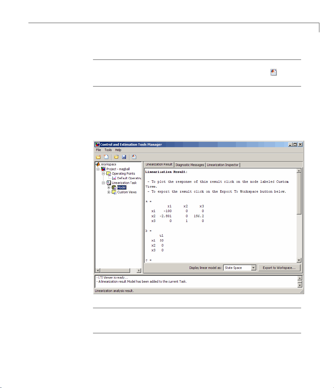
7 View the state-space matrices of the linearization result by selecting the

Model node under the Linearization Task node.

This action opens the Linearization Results tab shown in the following
figure.

Tip To display linearization results using a different mathematical form,
such as zero-pole-gain or transfer function, select the corresponding option
from the Display linear model as list.

4-15

4 Tutorial — Linearizing a Plant in a Single-Loop Control System Using the GUI

8 Save the Control and Estimation Tools Manager project, which contains

the linearization results.

a In the Co ntrol and E s timation Tools Manger, select File > Save.

This action opens the Save Projects dialog box.

4-16

b In the S

ave Projects dialog box, click OK.

This action opens the Save Projects window.

c In the Save Projects window, enter a project name, and click Save.

This action saves the project as a MAT-file.

Tip You can load this project by selecting File > Load in the Control and
Estimation Tools Manager.

Tutorial — Linearizing
a Plant in a Single-Loop
Control System Using the
Command Line

• “About This Tutorial” on page 5-2

• “Linearizing the Magnetic Ball P lant” on page 5-6

5

5 Tutorial — Linearizing a Plant in a Single-Loop Control System Using the Command Line

About This Tutorial

In this section...

“Objectives” on page 5-2

“About the Model” on page 5-2

Objectives

In this tutorial, you learn how to use Simulink Control Design functions at the
command line to linearize a nonlinear plant in a single-loop control system
about the existing operating point in the Simulink model.

About the Model

• “The magball Simulink Model” on page 5-2

• “Magnetic Ball Plant Subsystem” on page 5-3

5-2

The magball Simulink Model

The magball Simulink model shown in the following figure contains the
nonlinear Magnetic Ball Plant and a controller in a single-loop feedback
system.

About This Tutorial

To view the model of the Magnetic Ball Plant subsystem, double-click the
corresponding block in the

magball model. The blocks in this model represent

the mathematical system described in “Magnetic Ball Plant Subsystem” on
page 5-3.

For information about creating Simulink m od el s, see “Creating a Simulink
Model”.

Magnetic Ball Plant Subsystem

The Magnetic Ball Plant subsystem of the magball model is shown in the
following figure.

5-3

5 Tutorial — Linearizing a Plant in a Single-Loop Control System Using the Command Line

The Magnetic Ball Plant model represents an iron ball of mass M.Thisball
moves under the influence of the gravitational force, Mg,andaninduced

5-4

2



magnetic force,
magnetic force results in a nonlinear plant.

The inductor in the electric circuit, shown in the following figure, causes the
induced magnetic force. This circuit also includes a voltage source and a
resistor.

i

. The presence of the squared term in the induced

h

About This Tutorial

The following table describes the variables, parameters, differential
equations, states, inputs, and outputs of the Magnetic Ball Plant subsystem.

Variables

Parameters

Differential
equations

h is th e height of the ball.

i is the current.

V is the voltage in the circuit.

M is the mass of the ball.

g is the gravitational acceleration.

β is a constant related to the magnetic force.

L is the inductance of the coil.

R is the resistance of the circuit.

The height of the ball, h, is described in the following
equation:

M

2

dh

=−

2

dt

Mg

2



i

h

The current in the circuit, i, is described in the following
equation:

di

L

dt

ViR=−

States

Inputs V

Outputs

h

dh/dt

i

h

5-5

5 Tutorial — Linearizing a Plant in a Single-Loop Control System Using the Command Line

Linearizing the Magnetic Ball Plant

In this section...

“Why Linearize a Nonlinear Plant?” on page 5-6

“Overview of the Linearization Process” on page 5-6

“How to Linearize the Magnetic Ball Plant” on page 5-7

Why Linearize a Nonlinear Plant?

Linearization is a linear approximation of a nonlinear system, based on the
assumption that the system is approximately linear within a specific range of
operation. This approximation is valid in a small region around the operating
point of the system. An operating point is a set of inputs, o u t pu ts, and states
that describe the operating conditions of a system. For more information
about operating points and how they impact linearization, see “Why Are
Operating Points Important?”.

5-6

In real-world problems, models are nonlinear. Because you need a linear,
time-invariant model for most control design and analysis applications, you
must linearize a nonlinear model before you can accomplish these goals.

For mo re information about linearization, see “What Is Linearization?”.

Overview of the Linearization Process

The process for linearizing the Magnetic Ball Plant in this tutorial includes
the following tasks:

• Defining the portion of the model to linearize, also known as the

linearization path.

• Removing the effects of a feedback loop in a single-loop control system.

• Linearizing about the existing operating point in the Simulink model.

• Viewing the linearization results in a step response plot and as state-space

equations.

Linearizing the Magnetic Ball P lant

How to Linearize

1 Open the magneti

Command Window

magball

the Magnetic Ball Plant

c ball model by typing the following in the MATLAB

:

The model opens in Simulink as shown in the following figure.

2 Define the portion of the model to linearize using the linio command.

a Insert a linearization input point before the Magnetic Ball Pla n t by

typing the following command:

magball_io(1)=linio('magball/Controller',1,'in')

This command creates the magball_io linear ization I/O obj ect in the
MATLAB workspace. This object contains a linearization I/O setting
for the input point.

Linearization IOs:

--------------------------

Block magball/Controller, Port 1 is marked with the following properties:

5-7

5 Tutorial — Linearizing a Plant in a Single-Loop Control System Using the Command Line

- No Loop Opening

- An Input Perturbatio n

- No signal name. Linearization will use the block name

b Insert a

typing t

linearization output point after the Magnetic Ball Plant by

he following command:

magball_io(2)=linio('magball/Magnetic Ball Plant',1,'out')

This command updates the magball_io object to include a second
linearization I/O setting for the output point.

Linearization IOs:

--------------------------

Block magball/Controller, Port 1 is marked with the following properties:

- No Loop Opening

- An Input Perturbatio n

- No signal name. Linearization will use the block name

Block magball/Magnetic Ball Plant, Port 1 is marked with the following properties:

- An Output Measuremen t

- No Loop Opening

- No signal name. Linearization will use the block name

3 Remove the effects of the feedback loop for open-loop analysis by typing the

following command:

magball_io(2).OpenLoop='on'

This command updates the magball_io object to include a loop opening at
the output signal of t h e Magnetic Ball Plant. Opening the loop ensures that
the linearization result includes only theplantwhilepreservingthemodel
operating point. For more information on the effects of a feedback loop on
linearization results, see “Performing Open-Loop Analysis”.

5-8

Linearization IOs:

--------------------------

Block magball/Controller, Port 1 is marked with the following properties:

- No Loop Opening

- An Input Perturbatio n

- No signal name. Linearization will use the block name

Linearizing the Magnetic Ball P lant

Block magball/Magnetic Ball Plant, Port 1 is marked with the following properties:

- An Output Measuremen t

- A Loop Opening

- No signal name. Linearization will use the block name

4 Perform the linearization using the l inea rize command by typing the

following:

magball_lin=linearize('magball',magball_io)

This command linearizes the portion of the model defined in the m agba ll_io
object about the operating point currently specified in the model. This
command returns the following linearization result as a state-space object.

a=

magball/Magn magball/Magn magball/Magn
magball/Magn001
magball/Magn 0 -100 0
magball/Magn 196.2 -2.801 0

b=

magball/Cont
magball/Magn 0
magball/Magn 50
magball/Magn 0

c=

magball/Magn magball/Magn magball/Magn
Magnetic Bal100

d=

magball/Cont
Magnetic Bal 0

Continuous-time model.

5 View the step response of the linearized model by typing the following

command:

ltiview(magball_lin)

5-9

5 Tutorial — Linearizing a Plant in a Single-Loop Control System Using the Command Line

This command opens the LTI Viewer GUI, which displays the step response
plot of the linear model.

5-10

The step response decreases exponentially after about 0.8 seconds, which
indicates that the plant model is unstable. The linear model provides an
accurate approximation of the nonlinear Magnetic Ball Plant, which is
also unstable.

Tip You can use the right-click menu of the LTI Viewer GUI to display
a different plot or add characteristics to the response plot, such as peak
response and settling time. For more information about working with
response plots, see “LTI Viewer” in the Control System Toolbox Getting
Started Guide.

Tip For information about designing a stabilizing controller for the
Magnetic Ball Pla n t, see “Designing Compensators”.

Linearizing the Magnetic Ball P lant

6 Save the linearized model and I/O object of the magball model using the

save command by typing the following:

save magball_project magball_lin magball_io

This command creates a file named magball_project. mat in the current
folder.

Tip You can use the load command to reload this project.

5-11

5 Tutorial — Linearizing a Plant in a Single-Loop Control System Using the Command Line

5-12

Tutorial — Designing
a Compensator Using
Classical PID Techniques

• “About This Tutorial” on page 6-2

• “Designing a PID Compensator Using the Robust Response Time Tuning

Algorithm” on page 6-8

• “Tuning the PID Compensator Using Bode Graphical Tuning” on page 6-17

6

• “Simulating the Closed-Loop Simulink Model” on page 6-22

6 Tutorial — Designing a Compensator Using Classical PID Techniques

About This Tutorial

In this section...

“Objectives” on page 6-2

“About the Model” on page 6-2

“Requirements for the Compensator Design” on page 6-6

“Overview of the Compensator Design Process” on page 6-6

Objectives

In this tutorial, you learn how to use the Simulink Control Design GUI to
design a PID compensator for a single-loop feedback system that is operating
at the operating conditions specified in the Simulink model. You accomplish
the following tasks:

• Configure the model and GUI for compensator design.

6-2

• Design a PID compensator using the robust response time tuning algorithm

and Bode graphical design.

• Simulate the closed-loop nonlinear model.

About the Model

• “The watertank_comp_design Simulink Model” on page 6-3

• “Water-Tank Subsystem” on page 6-3

• “Controller Subsystem” on page 6-6

About This Tutorial

The watertank_comp_design Simulink Model

The watertank_comp_design model, shown in the following figure, contains
the Water-Tank System plant and a simple proportio nal-integral-de riv ative
(PID) controller, called Controller, in a single-loop feedback system.

To view the Water-Tank System and the Controller, double-click the
corresponding subsystem in the
descriptions of these subsystems, see the following topics:

• “Water-Tank Subsystem” on page 6-3

• “Controller Subsystem” on page 6-6

For information about creating Simulink m od el s, see “Creating a Simulink
Model”.

watertank_comp_design model. For

Water-Tank Subsystem

The Water-Tank subsystem of the watertank_comp_design model appears in
the following figure.

6-3

6 Tutorial — Designing a Compensator Using Classical PID Techniques

This model represents the water-tank system depicted in the following figure.

6-4

Water enters the tank from the top at a rate proportional to the voltage, V,
applied to the pump. The water leaves through an opening in the tank base
at a rate that is proportional to the square root of the water height, H,in
the tank. The presence of the square root in the water flow rate results in a
nonlinear plant.

The following table describes the variables, parameters, differential
equations, states, inputs, and outputs of the water-tank system.

About This Tutorial

Variables

Parameters

Differential equation

States

Inputs V

H is the height of water in the tank.

Vol is the volume of water in the

tank.

V isthevoltageappliedtothepump.

A is the cross-sectional area of the

tank.

b is a constant related to the flow
rate into the tank.

a is a constant related to the flow
rate out of the tank.

H

d

Vol A

dt

dH

dt

bV a H==−

6-5

6 Tutorial — Designing a Compensator Using Classical PID Techniques

Outputs

H

Controller Subsystem

The Controller subsystem appears in the following figure.

This mod
water in

Requir

The com
System

el contains a PID Controller block that controls the height of the

the Water-Tank System.

ements for the Compensator Design

pensator you design in this tutorial must control the Water-Tank

response as follows:

6-6

• The ov

• The ri

Over

The p
tut

• Con

• De

al

ershoot is l ess than 5%.

se time is less than 5 seconds.

view of the Compensator Design Process

rocess for designing a compensator for the Water-Tank System in this

orial includes the following tasks:

figuring the model andGUIforthedesign.

signing a PID compensator using the robust response time tuning

gorithm.

About This Tutorial

• Tuning the compensator using the Bode design technique.

• Simulating the closed-loop Simulink model with the compensator design to

analyze the system dynamics.

Simulink Control Design tools support linear control design. Although
the Water-Tank System is nonlinear, you do not need to linearize this
nonlinear plant model as a separate step–Simulink Control Design software
automatically linearizes the model about the model operating point when
you do not specify a different operating point. Th e linearization provides a
valid a ppro ximation of the nonlinear model in a region around the operating
point. For more information about linearization and how the operating point
impacts linearization results, see “What Is Linearization?” and “Why Are
Operating Points Important?”

6-7

6 Tutorial — Designing a Compensator Using Classical PID Techniques

Designing a PID Compensator Using the Robust Response
Time Tuning Algo

rithm

In this portion
PID robust resp
by The MathWor
phase margin.

To design a PI

1 Open the wate

the MATLAB C

watertank_comp_design

The comman
showninth

of the tutorial, you design a compensator using the autom ate d

onse time tuning algorithm. This tuning method, developed

ks,tunes the PID gains to maximize bandwidth and optimize

D compensator:

rtank_comp_design

dopensthe

efollowingfigure.

modelbytypingthemodelnamein

ommand Window:

watertank_comp_design model in Simulink, as

6-8

e

2 In th

Des

This action opens the Control and Estimation Tools Manager with the
Simulink Compensator Design Task node selected.

watertank_comp_design model window, select Tools > Control

ign > Compensator Design.

Designing a PID Compensator Using the Robust Response Time Tuning Algorithm

3 Select the PID Controller block as the block to tune.

a In the Tunable Blocks tab, click Select Blocks.

This ac

b In the w

c Selec

tion opens the Select Blocks to Tune window.

atertank_comp_design tree, select the Controller subsystem.

ttheTune? checkbox for PID Controller.

6-9

6 Tutorial — Designing a Compensator Using Classical PID Techniques

d Click OK.

4 Define the closed-loop systems for which you want to analyze the response.

6-10

The input and output points of the closed-loop path are already defined in
the

watertank_comp_design model. If you needed to add or define them,

you would use the following steps:

a In the watertank_comp_design model, right-click the output of the

Desired Water Level block, and select Linearization Points > Input
Point.

This action displays the

symbol on the signal line. This symbol

indicates the input of the closed-loop path.

b Right-click the output signal from the Water-Tank System, and select

Linearization Points > Output Point.

This action displays the

symbol on the signal line. This symbol

indicates the output of the closed-loop path.

Designing a PID Compensator Using the Robust Response Time Tuning Algorithm

The Simulink model now resembles the following figure.

5 In the Control and Estimation Tools Manager, click Tune Blocks to open

the Design Configuration Wizard. Click Next.

6 Step 1 of the Design Configuration Wizard prompts you to select the design

plotsyouwillusetotunethecontroller. Accept the d efault settings and
click Next.

7 In Step 2 of the Design Configuration Wizard, specify the type of plot for

analyzing the response.

a In the Analysis Plots area, select Step for the Plot Type corresponding

to Plot 1.

b In the Plots section of the Contents in Plots pane, select 1 fo r Closed

Loop from Step to Water-Tank System.

6-11

6 Tutorial — Designing a Compensator Using Classical PID Techniques

8 Click Finish.

6-12

The software performs the following actions:

• Linearizes the Simulink model about the operating point specified in

the model.

• Creates a SISO Design Task node under the Simulink Compensator

Design Task node.

• Opens the following plot windows:

– LTI Viewer for SISO Design Task window, which shows the

closed-loop Step Response plot of the linearized model

– SISO Design for SISO Design Task window, which is empty

You do not use in this window in this section of the tutorial. Keep this
window open for the next section of the tutorial.

The Control and Estimation Tools mana ger resembles the following figure.

Designing a PID Compensator Using the Robust Response Time Tuning Algorithm

The Step Response plot shows an overshoot that does not mee t the
overshoot design requirement of less than 5%.

6-13

6 Tutorial — Designing a Compensator Using Classical PID Techniques

6-14

9 In the A utomated Tuning tab of the SISO Design Task node in the

Control and Estimation Tools Manager, select
method.

10 In the Specifications area, select the following options:

• Controller type:

• Tuning algorithm: Robust response time

PI

PID Tuning as the Design

Designing a PID Compensator Using the Robust Response Time Tuning Algorithm

11 Click Upd

ate Compensator.

This action computes the PI values for the compensator using the robus t
response time tuning algorithm and updates the Step Response plot.

Tip You can view the PI values in the Parameter tab of the Compensator
Editor tab in the SISO Design Task node.

12 Evaluate whether the compensator design meets the design requirements

by analyzing the overshoot and the rise time, as follows:

a Right-click the Step Response plot and select the following options:

• Characteristics > Peak Response

• Characteristics > Rise Time

These actions add a plot marker to the plot for each characteristic,
shown as blue dots.

b Left-click each blue dot to open the corresponding data marker.

6-15

6 Tutorial — Designing a Compensator Using Classical PID Techniques

The data markers show the following response characteristics:

• The overshoot is 11.6%.

• The rise time is 82.2 seconds.

6-16

This sy
allowe
rise t

You decrease the rise time by increasing the gain of the compensator, as
described in “Tuning the PID Compensator Using Bode Graphical Tuning”
on page 6-17.

stem response with the PID compensator exceeds the maximum

d overshoot of 5%. The rise time is much slower than the required

ime of 5 seconds.

Tuning the PID Compensator Using Bode Graphical Tuning

Tuning the PID Compensator Using Bode Graphical Tuning

In this portion of the tutorial, you decrease the rise time of the Water-Tank
System response by incre as ing the gain in the compensator using Bode
graphical tuning. Bode graphical tuning lets you design a compensator by
manipulating Bode diagrams of the open-loop response. This process is also
called loop shaping.

You must have already designed an initial compensator using PID tuning,
as described in “Designing a PID Compensator Using the Robust Response
Time Tuning Algorithm” on page 6-8.

To design a compensator using Bode graphical tuning:

1 In the Control and Estimation Tools Manager, select the Graphical

Tuning tab of the SISO Design Task node.

2 In the Plot Type cell that corresponds to Plot 1, select Open-Loop Bode.

6-17

6 Tutorial — Designing a Compensator Using Classical PID Techniques

6-18

This action creates an Open-Loop Bode plot in the S ISO Design for SISO
Design Task window. This plot shows a Bode plot of the linearized m o del
with the compensator designed using automated PID tuning.

Tuning the PID Compensator Using Bode Graphical Tuning

3 IntheSISODesignwindow,dragtheBodeMagnitudelineupwardto

increasethegain. Asyouadjustthegain,viewtheaffectsontheclosed-loop
response in the Step Response plot.

By increasing the gain, you increase the bandwidth and speed up the
response. One possible compensato r design that meets the tutorial
requirements has the following parameters:

• P=

5.0368

• I=0.11434

• D=0

6-19

6 Tutorial — Designing a Compensator Using Classical PID Techniques

Tip You can view the parameter values corresponding to the gain

adjustment you made in the Bode Magnitude plot in the Compensator
Editor tab of the SISO Design Task. You can also adjust the parameter

values in this tab.

4 Evaluate whether the compensator design meets t he design requirements

by analyzing the overshoot and the rise time, as follows:

a Right-click the Step Response plot and select the following options, if you

have not done so already:

• Characteristics > Peak Response

• Characteristics > Rise Time

These actions add a plot marker to the plot for each characteristic,
shown as blue dots.

b Left-click each blue dot to open the corresponding data marker.

6-20

The data markers show the following response characteristics:

• The overshoot is 0.437%.

• The rise time is 1.72 seconds.

Tuning the PID Compensator Using Bode Graphical Tuning

This compensator design satisfies the design requirements of less than 5%
overshoot and less than 5 second rise time.

6-21

6 Tutorial — Designing a Compensator Using Classical PID Techniques

Simulating the Closed-Loop Simulink Model

In this portion of the tutorial, you simulate th e nonlinear closed-loop Simulink
model that includes a PID com pensator to determine if the design meets
the requirements.

You must have already designed the compensator, a s described in “Tuning
the PID Compensator Using Bode Graphical Tuning” on page 6-17.

To simulate the model:

1 In the Control and Estimation Tools Manager SISO Design Task node,

click Update Simulink Block Parameters.

This action writes the compensator parameters into the PID Controller
block of the Controller subsystem in the Simulink model.

Tip You can view the PID Controller block parameters in the Function
Block Parameters Dialog box. To open this dialog box, double-click the
PID Controller block.

6-22

Simulating the Closed-Loop Simulink®Model

2 In the Simulink model, double-click the Scope block to open the Scope block

window.

3 In the Simulink model, click to simulate the model. Then, click

to autoscale the axis.

6-23

6 Tutorial — Designing a Compensator Using Classical PID Techniques

This action
model with t
is less tha
design mee
second ris

n 5 seconds and there is minimal overshoot. Thus, this compensator

etime.

updates the Scope window with the response of the nonlinear

he compensator design. This simulation shows that the rise time

ts the requirements of less than 5% overshoot and less than 5

6-24