Mathworks SIMULINK CONTROL DESIGN 3 user guide

Download

Simulink®Control

User’s Guide

Design™ 3

How to Contact The MathWorks

www.mathworks. comp.soft-sys.matlab Newsgroup www.mathworks.com/contact_TS.html T echnical Support

suggest@mathworks.com Product enhancement suggestions

bugs@mathwo doc@mathworks.com Documentation error reports service@mathworks.com Order status, license renewals, passcodes

info@mathwo

com

rks.com

Web

Bug reports

Sales, prici

ng, and general information

508-647-7000 (Phone)

508-647-7001 (Fax)

The MathWorks, Inc. 3 Apple Hill Drive Natick, MA 01760-2098

For contact information about worldwide offices, see the MathWorks Web site.

Simulink

The software described in this document is furnished under a license agreement. The software may be used or copied only under the terms of the license agreement. No part of this manual may be photocopied or reproduced in any form without prior written consent from The MathW orks, Inc.

FEDERAL ACQUISITION: This provision applies to all acquisitions of the Program and Documentation by, for, or through the federal government of the United States. By accepting delivery of the Program or Documentation, the government hereby agrees that this software or documentation qualifies as commercial computer software or commercial computer software documentation as such terms are used or defined in FAR 12.212, DFARS Part 227.72, and DFARS 252.227-7014. Accordingly, the terms and conditions of this Agreement and only those rights specified in this Agreement, shall pertain to and govern theuse,modification,reproduction,release,performance,display,anddisclosureoftheProgramand Documentation by the federal government (or other entity acquiring for or through the federal government) and shall supersede any conflicting contractual terms or conditions. If this License fails to meet the government’s needs or is inconsistent in any respect with federal procurement law, the government agrees to return the Program and Docu mentation, unused, to The MathWorks, Inc.

Trademarks

MATLAB and Simulink are registered trademarks of The MathWorks, Inc. See

www.mathworks.com/trademarks for a list of additional trademarks. Other product or brand

names may be trademarks or registered trademarks of their respective holders.

Patents

The MathWorks products are protected by one or more U.S. patents. Please see

www.mathworks.com/patents for more information.

Control D es ign ™ User’s G uid e

Revision History

June 2004 Online only New for V ersion 1.0 (Release 14) October 2004 Online only Revised for Version 1.1 (Release 14SP1) March 2005 Online only Revised for Version 1.2 (Release 14SP2) September 2005 O nline only Revised for Version 1.3 (Release 14SP3) March 2006 Online only Revised for Version 2.0 (Release 2006a) September 2006 O nline only Revised for Version 2.0.1 (Release 2006b) March 2007 Online only Revised for Version 2.1 (Release 2007a) September 2007 O nline only Revised for Version 2.2 (Release 2007b) March 2008 Online only Revised for Version 2.3 (Release 2008a) October 2008 Online only Revised for Version 2.4 (Release 2008b) March 2009 Online only Revised for Version 2.5 (Release 2009a) September 2009 O nline only Revised for Version 3.0 (Release 2009b) March 2010 Online only Revised for Version 3.1 (Release 2010a)

Working with Simulink®Control Design

Creating or Opening a Simulink Model .............. 1-2

Details of Possible Models Example Model: The Magnetic Ball System

.......................... 1-2

............ 1-2

Contents

Projects

BeginningaProject

Creating a Simulink Creating an Operating Points Task Creating a Linearization Task Creating a Simulink Compensator Design Task

Saving Projects

Opening Previously Saved Projects

Exporting Results

Exporting Linearization Results Exporting Compensator Designs Exporting Operating Points ExportingandRestoringLinearization I/O Settings

................................ 1-7

Control Design Project ........... 1-7

.................................... 1-11

................................. 1-13

Operating Point Analysis Using the GUI

................... 1-8

....................... 1-8

......... 1-10

................. 1-12

..................... 1-13

..................... 1-14

......................... 1-15

..... 1-15

What Are Operating Points? ........................ 2-2

Definition of an Operating Point Equilibrium Operating Points Simulink Model Operating Points

..................... 2-2

....................... 2-2

.................... 2-3

Why Are Operating Points Important? ............... 2-6

Impact of Operating Points Choosing an Operating Point for Accurate Linearization

......................... 2-6

.. 2-7

Ways to Create Operating Points

Creating Operating Points

Simulink Computing Operating Points from S pecifications Specifying Operating Points from Known Values Extracting Operating Points From Simulation Computing Equilibrium Operating Points

Working with Operating Points

Copying Operating Points Exporting Operating Points Saving Operating Points Importing Operating Points Importing Initial Values Constraining Outputs Changing Optimization Settings

Recommendations for Computing Operating Points

How to Create Accurate Operating Points Impact of Blocks on the Simulink M odel Operating

Point Computing Operating Points for SimMechanics Models Choosing Initial Values for Computing Operating

Points Computing Operating Points for B l ock s with Special

Behavior

Control D esign De fa ult Opera t in g Point ...... 2-10

........................... 2-23

............................ 2-25

............................ 2-26

.............................. 2-27

......................................... 2-31

......................................... 2-37

...................................... 2-38

.................... 2-9

......................... 2-10

........ 2-10

........ 2-15

.......... 2-17

............. 2-22

..................... 2-23

......................... 2-24

......................... 2-25

..................... 2-27

............. 2-31

.. 2-31

.. 2-36

vi Contents

Operating Point Analysis Using the Command

Line

Overview ......................................... 3-2

Example: Water-Tank System ....................... 3-3

Water-Tank System Model Equations

............................... 3-3

.................................. 3-4

Creating or Opening a Simulink Model

Computing Operating Points from Specifications

Workflow for Computing Operating Points from

Specifications Creating an Operating Poin t Specification Object Configuring the Operating Point Specification Object Computing the Complete Operating Point Alternative Method for Specifying Initial Guesses Adding Output Constraints to Specifications

Specifying Completely Known Operating Points

Workflow for Specifying Completely Known O pe rating

Points Creating an Operating Point Object Changing Operating Point Values

Extracting Values from Simulation

Using Structures and Vectors of Operating Point

Values

......................................... 3-14

.......................................... 3-17

.................................. 3-7

.................... 3-15

.............. 3-5

............. 3-10

........... 3-12

.................. 3-14

.................. 3-16

..... 3-7

....... 3-7

.... 3-8

....... 3-11

...... 3-14

Exact Linearization Using the GUI

What Is Linearization? ............................. 4-2

Linearization Background Analytic Repre sentations of Linear Models

Ways to Linearize Models

Steps for Linearizing Models Using the GUI

.......................... 4-2

............. 4-3

.......................... 4-7

.......... 4-8

vii

Choosing Linearization Settings and Algorithms ..... 4-9

HowtoChooseLinearizationSe tti ngs and Algorithms Options for Linearization Algorithm Method Block-by-Block Analytic Linearization Numerical-Perturbation Linearization Changing State Ordering in the Linearized Model

Configuring the Linearization of Specific Blocks and

Subsystems

Ways to Configure Blocks and Subsystems For

Linearization

Controlling the Analytic Linearization of Individual

Blocks Specifying the Linearization of Blocks and Subsystems Controlling the Block Perturbation Linearization of

Individual Blocks

Selecting Inputs and Outputs for the Linearized

Model

What are Linearization Points? Inserting Linearization Points Removing Linearization Points Performing Open-Loop Analysis Inspecting Analysis I/Os

..................................... 4-36

................................... 4-36

........................................ 4-36

............................... 4-40

.......................................... 4-45

...................... 4-45

....................... 4-46

...................... 4-48

..................... 4-49

............................ 4-52

........... 4-11

................ 4-12

................ 4-24

... 4-9

....... 4-34

... 4-37

viii Contents

Linearizing a Block

Linearizing the Model

Linearizing at an Operating Poin t Creating Other Types of Linear Models Linearizing Discrete-Time and Multirate M odels

Viewing Linearization Results

Using the LTI Viewer Displaying Linearization Results Highlighting Blocks in the Linearization Inspecting the Linearization Results Block by Block Comparing the Results of Multiple Linearizations

Validating Exact Linearization Results

Ways to Validate Exact Linearization Results

................................ 4-55

.............................. 4-57

.................... 4-57

............... 4-64

...................... 4-66

.............................. 4-66

..................... 4-66

.............. 4-68

.............. 4-76

........ 4-65

..... 4-69

....... 4-71

.......... 4-76

Creating Input Signals for Validation ................. 4-76

Frequency-Domain Validation Time-Domain Validation

....................... 4-77

........................... 4-80

Troubleshooting Exact Linearization Results

Diagnosing Blocks Troubleshooting Your Model at the Subsystem and Block

Level Troubleshooting L ine arization Settings Troubleshooting Models with Events-Based Subsystems Troubleshooting Yo ur Operating Point

......................................... 4-86

................................. 4-82

............... 4-87

................ 4-88

Exact Linearization Using the Command Line

Steps for Linearizing Models Using the Command

Line

Configuring the Linearization for Specific Blocks and

Subsystems

Selecting Inputs and Outputs for the Linearized

Model

Workflow for Selecting Inputs and Outputs Choosing and Storing Linearization Points Extracting Linearization Points from a Model Editing an I/O Object Open-Loop Analysis Using Functions

............................................ 5-2

..................................... 5-3

.......................................... 5-4

............. 5-4

.............................. 5-8

................. 5-10

........ 4-82

.. 4-88

............ 5-4

.......... 5-7

Linearizing the Model Using Functions

Linearizing the Model Linearizing Discrete-Time and Multirate M odels Computing Multiple Linearizations for Large Models

Analyzing th e Results U sing Functions

Options for Analyzing the Results Using the LTI Viewer Saving Your Work

.............................. 5-11

.................... 5-14

.............................. 5-14

................................. 5-16

.............. 5-11

.............. 5-14

........ 5-13

.... 5-13

Restoring Linearization I/O Settings .................. 5-16

Frequency Response Estimation of Simulink

About Frequency Response Estimation .............. 6-2

Using Frequency Response Models What Is a Frequency Response Model? Model Requirements Estimation Requires Input and Output Signals

............................... 6-4

................... 6-2

................ 6-2

........ 6-5

Models

Creating Input Signals for Estimation

Supported Input Signals Creating Sinestream Input Signals Creating Chirp Input Signals Modifying Input Signals

Estimating Frequency Response

Analyzing E stimated Frequency Response

Opening the Simulation Results Viewer Interpreting Frequency Response Analysis Plots Analyzing Simulated Output and FFT at Specific

Frequencies Annotating Frequency Response Estimation Plots Displaying Frequency Response of Multiple-Input

Multiple-Output (MIMO) Systems

Troubleshooting Frequency Response Estimation

When to Troubleshoot Time Respo nse Not at Steady State FFT Contains Large Harmonics at Frequencies Other than

the Inp u t Signal Frequency Time Response Grows Without Bound Time Respon se Is Discontinuous or Zero Time Respo n se Is Noisy

.................................... 6-25

............................ 6-7

........................ 6-14

............................ 6-16

.............................. 6-29

....................... 6-35

............................ 6-42

............... 6-7

................... 6-7

.................... 6-18

........... 6-22

............... 6-22

........ 6-23

....... 6-27

.................. 6-28

................... 6-29

................ 6-37

............... 6-39

.... 6-29

x Contents

Managing Estimation Speed and Memory ............ 6-51

Ways to Speed up Frequency Response Estimation Speeding Up Estimation Using Parallel Computing Managing Memory During Frequency Response

Estimation

..................................... 6-56

...... 6-51

Designing Compensators

Compensator Design Using Simulink ................ 7-2

..... 6-53

Automatic P ID Tuning

Automatic PID Tuning O v erview Designing Controllers with the PID Tuner Troubleshooting Automatic PID Tuning

Design and Analysis of Control Systems

Compensator Des ig n Process Overview Beginning a Compensator Design Task Selecting Blocks to Tune Selecting C lo sed-Loop Responses to Des ig n Selecting an Operating Point Creating a SISO Design Task Completing the Design

............................. 7-4

..................... 7-4

............. 7-6

............... 7-19

............. 7-27

................ 7-27

............................ 7-29

............ 7-32

........................ 7-34

........................ 7-37

............................. 7-48

Function Reference

Linearization Analysis I/Os ......................... 8-1

Operating Points

.................................. 8-2

Linearization

Frequency Response Estimation

...................................... 8-3

.................... 8-3

Functions — Alphabetical List

Block Reference

Linearization Example Using the Graphical

Interface

........................................ A-2

Examples

Linearization Example Using Functions

Frequency Response Estimation

.................... A-2

............. A-2

Index

xii Contents

Working with Simulink Control Design Projects

• “Creating or Opening a Simulink Model” on page 1-2

• “Beginning a Project” on page 1-7

• “Saving Projects” on page 1-11

• “Opening Previously Saved Projects” on page 1-12

• “Exporting Results” on page 1-13

1 Working with Simulink

Control Design™ Projects

Creating or Opening a Simulink Model

In this section...

“Details of Possible Models” on page 1-2

“Example Model: The Magnetic Ball System” on page 1-2

DetailsofPossibleModels

The first step in the linearization or compensator design process is to create or open a Simulink inputs and outputs (including none), and any number of states. The model can include user-defined blocks or S-functions. Your model can involve multiple compensators in addition to the plant, multiple feedback loops, and any number of subsystems.

Example Model: The Magnetic Ball System

This section introduces an example model, the magnetic ball system, that the remaining sections and chapters use to illustrate the process of linearizing a model or designing a compensator.

model of y our system. The model can have any number of

1-2

Magnetic Ball System

The electronic circuit in the following figure consists of a voltage source, a resistor, and an inductor in the form of a tightly wound coil. An iron ball beneath the inductor experiences a gravitational force as well as an induced magnetic force (from the inductor) that opposes the gravitational force.

Creating or Opening a Simulink®Model

Model Equations

Adiffer

where M is the mass of the ball, h is the height (position) of the ball, g is the acceleration due to gravity, i is the current, and β is a constant related to the magnetic force experienced by the ball. This equation describes the height, h, of the ball due to the unbalanced forces acting upon it.

The current in the circuit also varies with time and is given by the following differential equation

ential equation for the force balance on the ball is given by

di dt

=−

ViR=−

1-3

1 Working with Simulink

Control Design™ Projects

where L is the inductance of the coil, V is the voltage in the circuit, and R is the resistance of the circuit.

The system of equations has three states:

i,,

Thesystemalsohasoneinput(V), and o ne output (h). It is a nonlinear system duetothetermintheequationinvolvingthesquareofi and the inverse of h.

Due to its nonlinearity, you cannot analyze this system using methods for linear-time-invariant (LTI) systems such as step response plots, bode diagrams, and root-locus plots. However, you can linearize the model using the Simulink

Control Design™ software to approximate the nonlinear system as an LTI system. Linearization also occurs automatically when designing a compensator. This linearized system can then use the LTI Viewer for display and analysis and the SISO Design Tool for compensator design. Refer to for a discussion of the uses of linearized models and “What Is Linearization?” on page 4-2 for a discussion of the linearization process.

1-4

Opening the Model

To open the model for the magnetic ball example, type

magball

at the MATLAB®prompt. The magnetic ball system opens in the Simulink model viewer as shown in this figure.

Creating or Opening a Simulink®Model

The magball model consists of

• The magnetic ball system itself, within the sub system labeled Magnetic

Ball Plant.

• A Controller subsystem that controls the height of the ball by balancing

the forces acting on it.

• A reference signal that sets the desired height of the ball.

• A

Scope block that displays the height of the ball as a function of time.

Double-click a block to view its contents. The Controller block contains a zero-pole-gain model. The Magnetic Ball Plant block is shown in this figure.

1-5

1 Working with Simulink

Control Design™ Projects

1-6

The input to the Magnetic Ball Plant system, which is also the output of the Controller subsystem, is the voltage, V. The output is the height of the ball, h. The system contains three states within the three integrators:

dhdt,andCurrent.

Values of the parameters are given a s M=0.1 kg, g=9.81 m /s

height,

, R=2 Ohm,

L=0.02 H, and β=0.001.

Beginning a Project

In this section...

“Creating a Simulink®Control Design Project” on page 1-7

“Creating an Operating Points Task” on page 1-8

“Creating a Linearization Task” on page 1-8

“Creating a Simulink Compensator Design Task” on page 1-10

Creating a Simulink Control Design Project

With Simulink Co ntrol Design software you can create operating points, linearize, and design compensators for Simulink models. You perform all these tasks in a graphical environment called the Control and Estimation Tools Manager. The tasks are contained within a Control and Estimation Tools Manager project. Each project is associated with a single Simulink model and in addition to Simulink Control Design tasks, it can include tasks from other products such as the Simulink the Control System Toolbox™ product, and the Model Predictive Control Toolbox™ product.

Beginning a Project

Design Optimization™ product,

To open a new Simulink Control Design project:

1 Select Start > Simulink > Simulink Control Design > Linearization

Task or select Start > Simulink > Simulink Control Design > Simulink Compensator Design Task.

2 Enter a project name, select a model to analyze, and choose the tasks you

want to perform. Click OK to close the dialog box and open the new project.

Alternatively, you can create a new project from a Simul in k model window. Within the model window select Tools > Control Design > Linear Analysis to open a project containing a linearization task, or select Tools > Control Design > Control Design to open a project containing a compensator design task.

1-7

1 Working with Simulink

Control Design™ Projects

Creating an Oper

An Operating Poi automatically c

Compensator De

create operati

Creating a Lin

To create a li use one of the page 1-7 to ope task for thi

File>New>T

open the New that you wa

To open a ne lineariz

Analysis

Manager o followi

s project. To add a linearization task to an existing project, select

nt to open the task within, and then click OK.

w project within the Control and Estimation Tools Manager for

ation of the magball model, select Tools > Control Design > Linear

from the

pens and creates a new linearization task, as shown in the

ng figure.

nts node in the Control and Estimation Tools Manager is

reated when you begin a Linearization Task or a Simulink

sign Task.YoucanusetheOperating Points node to

ng points for a Simulink model.

earization Task

nearization task in the Control and Estimation Tools Manager,

methods in “Creating a Simulink

n a new project for your model, and choose a linearization

ask in the Control and Estimatio n Tools Manager window to

Task dialog box. Select Linearization Task and the project

magball window. The Control and Estimation Tools

ating Points Task

Control D es ign Project” on

1-8

Beginning a Project

The left pane of the Control and E stimatio n Tools Manager shows the project tree, w hich contains all your current projects. At this stage you should have just one project, Project - magball. Select a node within the tree to display its contents in the pane on the right.

1-9

1 Working with Simulink

Control Design™ Projects

View the default operating point and create new operating points.

Set up the linearization and inspect theresults listed in the Linearization Results pane.

Create customized plots of the linearization results.

• For information on the Operating Points node or the Operating Points

pane w ithin the Linearization Task node, refer to “Creating Operating Points” on page 2-10.

• For information on the Analysis I/Os pane within the Linearization

Task node, refer to “Selecting Inputs and Outputs for the Linearized

Model” on page 4-45.

1-10

• For information on the Linearization Results pane within the

Linearization Task node and inspecting linearization re sults, refer to

“Viewing Linearization Results” on page 4-66.

• For information on Custom Views, refer to “Viewing Linearization

Results” on page 4-66.

Creating a Simulink Compensator Design Task

To create a Simulink Compensator Design Task in the Control and Estimation Tools Manager, use one of the methods in “Beginning a Project” on page 1-7 to open a new project for your model, and choose a compensator design task for this project. To add a compensator design task to an existing project, select File>New>Taskin the Control and Estimation Tools Manager window to open the New Task dialog box. Select Simulink Compensator Design Task and the project that you want to open the task within, and then click OK.

Saving Projects

A Control and Estimation Tools Manager project can consist of multiple tasks such as linearization, compensator design, and operating points tasks as well as Simulink Design Optimization tasks and Model Predictive Control Toolbox tasks. Each task contains data, objects, and results for the analysis of a particular model.

1 To save a project as a MAT-file, select File > Save from the Control and

Estimation Tools Manager window.

Saving Projects

2 In the Save Projects dialog box, select one or m ore projects you want to

save. Youcansavemultipleprojects in one file. Click OK,andbrowseto the folder where you want to save the project. Enter the project name, and click Save.

1-11

1 Working with Simulink

Control Design™ Projects

Opening Previously Saved Projects

1 To open previously saved projects, select File > Load from the Control and

Estimation Tools Manager window. This opens the Load Projects dialog box.

1-12

2 Choose a project-file by either brows ing for the folder and file, or typing

the full path and filename in the Load from field. Project files are always MAT-files. After you specify the file, the projects contained in this file appear in the list. Select one or more projects in the list, and then click OK. When a file contains multiple projects, you can choose to load them all or just a few.

Exporting Results

In this section...

“Exporting Linearization Results” on page 1-13

“Exporting Compensator Designs” on page 1-14

“Exporting Operating Points” on page 1-15

“Exporting and Restoring Linearization I/O Settings” on page 1-15

Exporting Linearization Results

To export linearization results and the corresponding operating points, right-click the results node, Model,undertheLinearization Task node and select Export fromthemenu. IntheExportToWorkspacedialogbox, choose new names for the linearized model and operating point, or accept the defaults, and then click OK.

Exporting Results

The MATLAB workspace now contains two new objects, Model_op and

Model_sys.Toseethis,type

who

at the MATLAB prompt. This returns

Your variables are:

L Model_sys beta m Model_op R g

Alternatively, you can export the results to the MATLAB workspace by selecting File > Export from the LTI Viewer window or by clicking the

1-13

1 Working with Simulink

Control Design™ Projects

Export to Workspace button at the bottom of the L inearization Summary pane within the Model node.

By right-clicking the results node, Model, you can also de lete results.

Exporting Compensator Designs

To export a compensator design to the MATLAB workspace:

1 Select File > Export from the SISO Design Tool window.

2 In the SISO Tool Export dialog box, use the Select design list to choose

the design y ou want to export.

3 In the list, select the compensators to export, and then click either Export

to Workspace or Export to Disk.

1-14

Exporting Results

Exporting Operating Points

After creating operating points, you can use the Export To Workspace dialog box to export them for use outside of the Control and Estimation Tools Manager. You can use the exported operating point to perform analysis at the MATLAB command line or to initialize a model for simulation.

1 Under Select destination workspace, select either

• Base workspace to export the operating point to the MATLAB

workspace where you can use it with Simulink Control Design command-line functions

• Model workspace to export the operating poin t to the Mo d el workspace

where you can save it with the model for future use.

2 Enter a nam e for the exported operating point.

3 Select Use

to use the o inputs in

Data Impo

Simulink

Exporti

To expor

getlin

them in them to

For mo

setli

ng and Restoring Linearization I/O Settings

t linearization I/O settings to the MATLAB workspace, use the

function. You can save these settings using the save function. Use

a later session by reloading them with the

the model diagram with the

re information, see the function reference pages for

nio

the operating point to initialize model when you want perating point values as initial conditions for the states and

the model. The initial values are automatically set in the

rt/Export pane of the Configuration Parameters dialog box.

software uses these initial conditions when simulating the model.

load function. Upload

setlinio function.

getlinio and

1-15

1 Working with Simulink

Control Design™ Projects

1-16

Operating Point Analysis Using the GUI

• “What Are Operating Points?” on page 2-2

• “Why Are Operating Points Important?” on page 2-6

• “Ways to Create Operating Points” on page 2-9

• “Creating Operating Points” on page 2-10

• “Working with Operating Points” on page 2-23

• “Recommendations for Computing Operating Points” on page 2-31

2 Operating Point Analysis Using the GUI

What Are Operating Points?

In this section...

“Definition of an Operating Point” on page 2-2

“Equilibrium Operating Points” on page 2-2

“Simulink Model Operating Points” on page 2-3

Definition of an Operating Point

The operating point of a dynamic system defines its overall state at a given time. For example, in a model of a car engine, variable s such as engine speed, throttle angle, engine temperature, and surrounding atmospheric conditions typically describe the o perating point. It is important to specify the operating point accurately because it affects the system’s behavior. For example, the behavior of a car engine can vary greatly when it operates at high or low elevations.

2-2

Equilibrium Operating Points

An equilibrium operating point remains steady and constant with time; all states in the model are at equilibrium. It is also known as a steady state or trimmed operating point. For example, a car operating on cruise control on a flat road maintains a constant speed. Its operating point is steady, or at equilibrium.

A hanging pendulum provides an example of a stable equilibrium operating point. When the pendulum hangs straight down, its position does not change with time because it is at an equilibrium position. When its position deviates slightly fro m this position, it always returns to the equilibrium; small changes in the operating point do not cause the system to leave the region of good approximation around the equilibrium v alue.

A pendulum that points upward provides an example of an unstable equilibrium operating point. As long as the pendulum points exactly upward, it is steady at this equilibrium state. However, when the pendulum deviates slightly from this state, it swings downward and the operating point leaves the region around the equilibrium value.

What Are Operating Points?

Simulink Model O

This section inc

• “Operating Poi

• “Example of a S

ludes the following topics:

nt Versus Simulink Full-Model Operating Point” on page 2-3

imulink Model Operating Point” on page 2-4

perating Points

Operating Point Versus Simulink Full-Model Operating Point

The Simulink the b locks in GUI or the MAT you are actu operating p operating p

The follow full-mode

Makeup of

Block Types

Blocks value s

nport blocks with

level i

edatatype

doubl

full model operating point includes information from all of

a Simulink model. When you use the Simulink Control Design

LAB command line to create operating points for a model,

ally creating an operating point object (whatisreferredtoasthe oint). The operating point is a subset of the Simulink full-model oint.

ing table shows the different types of blocks that make up a

l operating point and which types are included in the operating point.

Simulink Full-Model Operating Point

Included in Operating Point?

Yes

with double

tates and root

Example of Block s

Integrator, State Space, Transfer Function, Inport

Root level inport blocks with nondouble or complex d ata type

Blocks with internal state representation that impacts block outputs

Source blocks with outputs specified by block dialog pa r ameters

Inport No

Backlash, Memory, Stateflow

Constant, Step

2-3

2 Operating Point Analysis Using the GUI

The operating point includes only the block information most comm only redefined by users. This information provides you with three places to make changes to the parameters of these common blocks in your model:

• Directly in the Simulink Control De sig n Control and Estimation Tools

Manager GUI

• At the MATLAB command line

• In the Simulink model

Note If you want to m ake changes to any block not included in the operating

point, you must m ake the changes directly in the Simulink model.

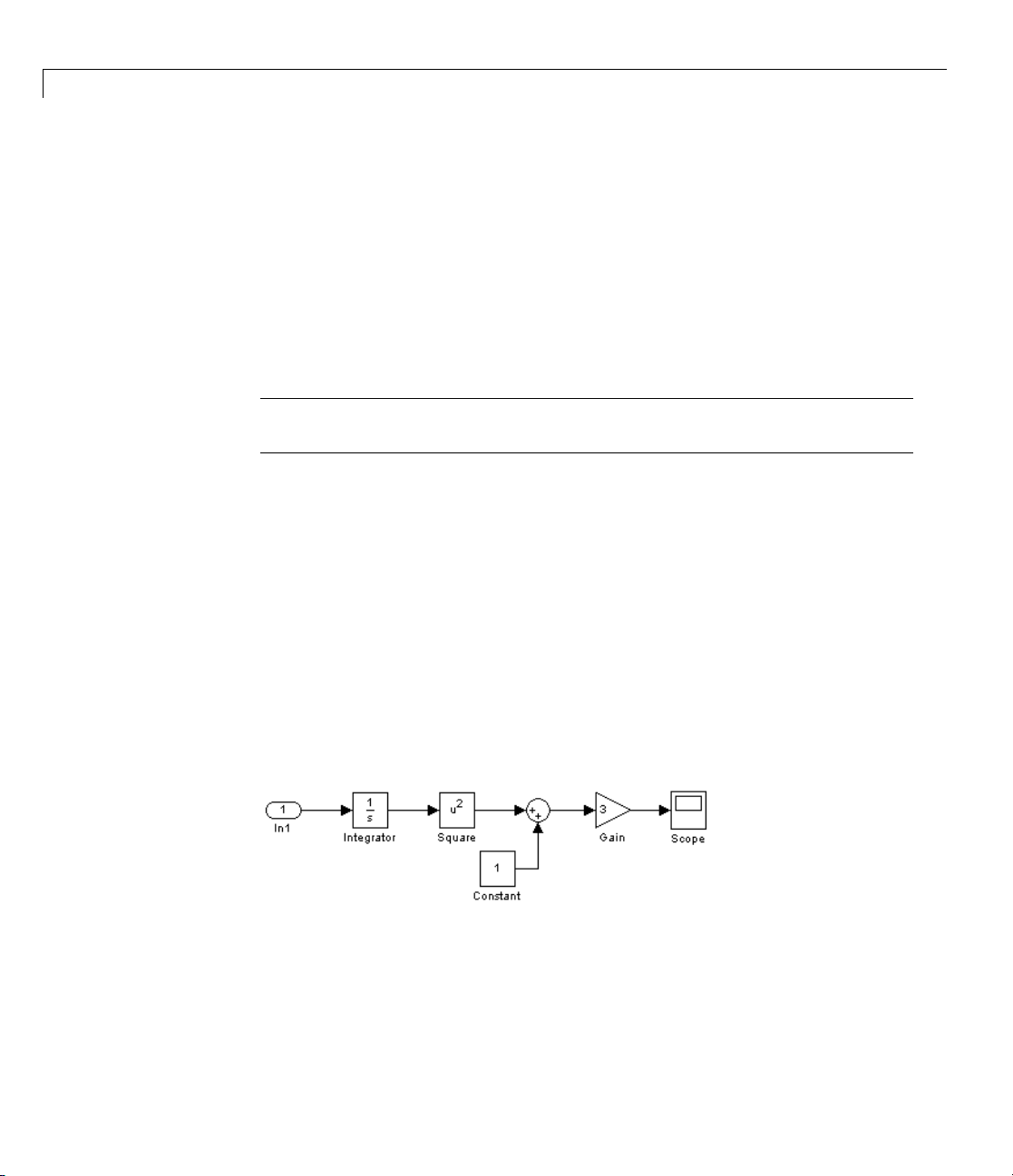
Example of a Simulink Model Operating Point

The following figure shows a simple Simulink model that has one block with state(theintegratorblock)andthereforeonestate, on the initial conditions set in the integrator block. The value of this state and the input from the inport block define the operating point in the Simulink Control Design software.

x1. This state depends

2-4

The square block output is derived from just the initial condition of the integrator block while the gain block has its output derived from both the initial condition of the integrator block and output of the constant block. The derivative dx/dt of the integrator block state is defined by the output level of therootinportblock.

tate,

The s

he model by propagating through the blocks in the model as follows.

in t

1 The

x1, defines the signal levels at the input and output of every block

integrator block initial condition of

x0 = 5 sets the state x1=5.

What Are Operating Points?

2 The state, x1, propagates in the direction of the arrows through the blocks

in the model, defining input and output signals on each block, as described in the following table.

Block Input Signal

Level

Square

Sum 25 from square,

Block Operation

squares

sums

Output Signal Level

1fromconstant

Gain

multiplies by 3

The following figure shows these input and output signal levels for each block.

2-5

2 Operating Point Analysis Using the GUI

Why Are Operating Points Important?

In this section...

“Impact of Operating Points” on page 2-6

“Choosing an Operating Point for Accurate L inearization” on page 2-7

Impact of Operating Points

A linearized model is an approximation that is valid in a region around the operating point of the syste m where the linearization took place. Near the operating point the approximation is good, while far away it may be poor. A linearized model of a car being operated at 3000 ft. is very accurate at elevations close to 3000 ft. but less accurate as the car travels higher or lower.

Example of a Linear Approximation of a Nonlinear Function

The following figure shows a nonlinear function,

functio functio approxi is poor The fol

linearization of

yx=−21

n about the operating point x=1, y=1. Near this operating point, the

mation is good. Away from this operating point, the approximation

. The precise boundaries of this region a re often somewhat arbitrary.

lowing figure shows a possible region of good approximation for the

. The linear function is an approximation to the nonlinear

yx=

,andalinear

2-6

Why Are Operating Points Important?

Choosing an Operating Point for Accurate Linearization

Your choice of operating point is important when you:

• Linearize a Simulink model. The choice of operating point determines the

accuracy of the linear approximation.

• Designing compensators with Simulink Control Design software. A

Compensator Design Task uses linearization when analyzing a Simulink model.

Tip Choose an operating point that is very close to the expected operating values of the system. One option is to use an equilibrium operating point, described in “Equilibrium Operating Points” on page 2-2.

2-7

2 Operating Point Analysis Using the GUI

Example of Linearization Results About Two Different Operating Points

A model can have two entirely different linearizations when the linearization is performed about different operating points. The following model can be linearized using the Simulink Control Design software.

The lineari

When this li nearization is performed about two different operating points, two different linearization results occur as shown in the following table.

Operating Point

Initial Condition = 5, State x1 =5

Initial Condition = 0, State x1 =0

Note The operating point consists of values for all the states in the model, although only those states between the linearization points are linearized. The whole model contributes to the operating point values of the states, inputs, and outputs of the portion of the model you are linearizing.

zation res ult for this model is shown in the following figure.

Linearization Result

30/s

2-8

Ways to Create Operating Points

You can compute operating points using any technique either:

• Interactively in the GUI

• Programmatically at the command line using MATLAB code

Tip You can automatically generate MATLAB code from your GUI

configuration.

Use the following table to choose a technique for creating operating points.

Ways to Create Operating Points

When you know...

Some values and constraints for inputs and states

Exact values for all inputs and states

Thetimeoreventinyourmodelto extractanoperatingpointduring simulation

Compute ope from...

Specifications

• GUI

• Command line

Known Values

• GUI

• Command line

Simulation

• GUI

• Command line

rating points

2-9

2 Operating Point Analysis Using the GUI

Creating Operating Points

In this section...

“Simulink®Control D esign Default Operating Point” on page 2-10

“Computing Operating Points from Specifications” on page 2-10

“Specifying O perating Points from Known Values” on page 2-15

“Extracting O perati ng Points From Simulation” on page 2-17

“Computing Equilibrium Operating Points” on page 2-22

Simulink Control Design Default Operating Point

A default operating point is automatically created and stored in a node in the project tree every time you open the Control and Estimation Tools Manag er unless you indicate otherwise. The default operating point consists of a snapshot of initial condition variables in the Simulink model. Initial condi tion variables are a special set of variables that can be set in the Simulink model. These variable include initial c onditions for blocks with state, such as the integrator o r state space blocks, and output values of root level inport blocks. F or more information on setting these variables, see “Importing and Exporting Data” in the Simulink User’s Guide.

2-10

By clicking on the Default Operating Point node, you can view these values and modify them for use in a linearization. The output levels for blocks like a constant block remain defined in the model.

Computing Operating Points from Specifications

You can specify target values or constraints on a subset of the model’s inputs, outputs, and states. The software uses numerical optimization methods to determine the full operating poin t based on this partial specification.

This section continues the magball example from “Creating a Linearization Task” on page 1-8. At this stage in the example, a linearization task has already been created for the model.

Creating Operating Points

You compute the operating point from specifications when you only know partial or implicit information. Typical operating point specifications search for steady state or equilibrium operating points.

2-11

2 Operating Point Analysis Using the GUI

1 Create a new operating point by either:

• Selecting the Operating Points node and then clicking the Compute

Operating Points tab

• Clicking the New Operating Point button on the Operating Points

pane of the Linearization Task node

2 From the Compute new operating points using li st, select operating

specifications

should now resemble the following figure.

Enter a known value or an initial guess in this column

. The Control and Estimation Tools Manager window

Select these check boxes when a steady-state

Select these check boxes when the operating point is known exactly

value is desired.

Enter maximum and minimum bounds on operating point values

2-12

Creating Operating Points

3 Enter operating point specifications in the table, such as any known values

or constraints on signal values. Switch between states, inputs, and outputs using the tabs on the left.

A suitable set of specifications for the

magball model is shown in the

following figure. This model does not contain any root-level input or output ports and, as a result, the Inputs and Outputs panes are empty. You can still constrain the output signal of any block by adding an Output Constraint linearizat ion point to the model . See “Constraining Outputs” on page 2-27 for information about adding an output constraint to the specifications for an operating point.

The height of the ball is known exactly (same as the reference signal height).

The ball height is 0.05 (same as the reference signal value). For a steady ball, use initial guess of 0 for dhdt. For the remaining states, choose arbitrary initial guesses.

A steady-state operating point is desired.

Use a minimum value of zero for the current (by convention current is positive when flowing clockwise around the circuit).

2-13

2 Operating Point Analysis Using the GUI

When y ou add states, inputs, or outputs to the model, or remove them from the model, click the Sync with Model button to update the operating pointtabletoreflectthesechanges.

4 Click Compute Operating Points. The Simulink Control Design software

finds an operating point that closely matches the specifications and adds the new operating point, labeled Operating Point,totheOperating Points node. Some specifications, even values specified as Known,may not be met exactly. Select the operating point in the project tree to view its contents and assess the results.

Actual dx values are small, because a a steady-state value was found.

2-14

For information on options that you can set when finding operating points from partial specifications, see “Changing Optimization Settings” on page 2-27.

Creating Operating Points

Note Inputs and o utputs for the operating point are not the same as the linearization input and output points, or analysis I/Os, used to define the inputs and outputs of the linearized model. Instead, operating-point inputs and outputs define the full operating point of a Simulink model, along with any additional, user-defined output constraints.

Tip To automatically generate MATLAB code that computes operating points as specified in the Control and Estimation Tools Manager, click

or select

File > Generate MATLAB Code.

Specifying Operating Points from Known Values

You can completely specify all inputs and states in the operating point.

This section continues the magball example from “Computing Operating Points from Specifications” on page 2 -10. At this stage in the example, a linearization task has already been created for the model, and a steady state operating point has been computed from specifications.

When you know the values of all states and inputs at the operating p oint, you can create a new operating point in the Control and Estim a tion Tools Manager and manually edit the operating point values:

1 Select the Operating Points node in the left pane and then click the

Operating Points tab in the right pane.

2 Click the New button in the bottom-right corner to create a new operating

point under the Operating Points node. This new operating point is labeled Default Operating Point (2).

2-15

2 Operating Point Analysis Using the GUI

3 View the details of DefaultOperatingPoint(2)(shown in the following

figure) by either:

• Selecting it under the Operating Points node in the project tree

• Selecting it in the Operating Points pane of the Linearization Task

node, and then clicking View

Enter known values of states and inputs at the operating point.

2-16

4 Edit the operating point by entering new values in the table. Switch

between state and input values using the tabs on the left.

Change the value of State-1 of Integrator to to

7. The model does not contain any root-level input ports, and, as a result,

-14 and the value of Current

the Inputs pane is empty.

When y ou add states, inputs, or outputs to the model, or remove them from the model, click the Sync with Model button to update the operating pointtabletoreflectthesechanges.

Creating Operating Points

5 Rename the operating point by right-clicking Default Operating Point

(2) under the Operating Points node, selecting Rename, and entering a

new name in the dialog box.

For example, label this operating condition Thepaneshouldnowresemblethefollowingfigure.

Known Operating Conditions.

o automatically generate MATLAB code that computes operating points

Tip T as specified in the Control and Estimation Tools Manager, click

File > Generate MATLAB Code.

or select

Extracting Operating Points From Simulation

You can create an operating point from a simulation of your model a t the following simulation points:

2-17

2 Operating Point Analysis Using the GUI

• Specified simulation times, such as when the simulation reaches a steady

state solution (see “Creating Operating Points at Specified Simulations Times” on page 2-18example in this section).

• Events during a specified simulation interval (see “Creating Operating

Points at Simulation Events” on page 2-21)

CreatingOperatingPointsatSpecifiedSimulationsTimes

Youcanextractanoperatingpointatspecifiedtimesduringasimulation of the model.

This section continues the magball example from “Specifying Operating Points from Known Values” on page 2-15. A t this stage in the example, a linearization task has already been created for the model, a steady state operating point has been computed from specifications, and a completely known operating point has been specified.

To create operating points at specified simulation times:

2-18

1 Open the Compute Operating Points tab by either:

• Selecting the Operating Points node in the project tree, and then

clicking the Compute Operating Points tab

• Clicking the New Operating Point button on the Operating Points

pane of the Linearization Task node

Creating Operating Points

2 From the Compute new operating points using list, select simulation

snapshots

. The window sho u ld now resemble the following figure.

3 Enter a vector of times in the Simulation snapshot times (sec) field.

Enter

[1,10] to compute operating points at t=1 and t=10.

4 Click Compute Operating Points. The Simulink Control Design software

simulates the model, extracts operating points, labeled Operating Point

2-19

2 Operating Point Analysis Using the GUI

at t=1 and Operating Point at t=10, and adds them to the Operating Points node in the project tree.

To view the contents of the operating point you created, select the operating point in the project tree as shown in this figure.

2-20

Note W them oper

To automatically generate MATLAB code that computes operating points

Tip

as specified in the Control and Estimation Tools Manager, click File > Generate MATLAB Code.

hen you add states, inputs, or outputs to the model, or remove

from the model, click the Sync with Model button to update the

ating point table to reflect these changes.

or select

Creating Operating Points

CreatingOperatingPointsatSimulationEvents

You can create an operating point from a simulation of your model at one or more of the following simulation events:

• Trigger-based events

• Function-call events

For more information about modeling events in Simulink models, see “Creating Conditional Subsystems” in the Simulink User’s Guide.

The Simulink Control Design software creates operating points at all simulation events within a specified simulation time.

Tocreateoperatingpointsatoneormoresimulationevents:

1 AddaTrigger-BasedOperatingPoint Snapshot block to your model. This

block is in the Simulink Control Design block library.

The model in the Trigger-Based O perating Point Snapshot demo shows the use of this block.

2 Select the Compute Operating Points tab in the Operating Points

node.

3 From the Compute new operating points using list, select simulation

snapshots

4 Enter a scalar value that specifies the simulation end time in the

Simulation snapshot times (sec.) field, shown in the following figure.

2-21

2 Operating Point Analysis Using the GUI

2-22

5 Click Compute Operating Points. The software simulates the model,

extracts operating points, and adds them to the Operating Points node in the project tree. Select an o perating point to view its contents and assess the results.

Computing Equilibrium Operating Points

You can use the software to compute equilibrium operating points. Follow the basic instructions in “Computing Operating Points from Specifications” on page 2-10. When you enter specifications in the States pane, select the Steady State check box at the top of the table. Selecting this check box causes the algorithm to look for an operating point in which all states are at equilibrium, or steady state.

Working with Operating Points

In this section...

“Copying Operating Points” on page 2-23

“Exporting Operating Points” on page 2-24

“Saving Operating Poin ts” on page 2-25

“Importing Operating Points” on page 2-25

“Importing Initial Values” on page 2-26

“Constraining Outputs” on page 2-27

“Changing Optimization Settings” on page 2-27

Copying Operating Points

In some situations you might want to create and edit a copy of an operating point. To create a copy of an operating point, right-click the operating point in the tree on the left, and select Duplicate from the right-click menu, as shown in the following figure.

Working with Operating Points

The new operating point appears beneath the original one in the tree. Click the new operating point to display i ts contents in the pane on the right. To change state or input values in the duplicated operating point, edit the values in the right pane. To change the name of the new operating point, right-click the operating point in the tree, select Rename from the right-click menu, and then enter a new name for the operating point.

2-23

2 Operating Point Analysis Using the GUI

Note that you cannot copy operating points that were computed from specifications. These operating points contain information related to the success of the optimization which would not be meaningful when the operating point values were changed.

Exporting Operating Points

After creating operating points using the Simulink Control Design software, you can export them from the Control and Estimation Tools Manager to the MATLAB workspace or the model workspace. You can use an exported operating point to perform analysis at the MATLAB command line or to initialize a Simulink model for simulation. To export an operating point, right-click the operating point under Operating Points in the pane on the left and select Export to Workspace. This opens the Export to Workspace dialog box, as shown below:

2-24

1 Click either

• Base Workspace to export the operating point to the MATLAB

workspace where you can use it with Simulink Control Design command-line functions

• Model Workspace to export the operating point to the Model workspace

where you can save it with the model for future use.

2 Enter a nam e for the exported operating point.

Working with Operating Points

3 Select Use the operating point to initialize model when you want

to use the operating point values as initial conditions for the states and inputs in the model. The initial values are automaticall y set in the Data Import/Export pane of the Configuration Parameters dialog box and Simulink uses these initial conditions when simulating the model.

Saving Operating Points

After you have exported the operating point to the MATLAB workspace, you can save it in a MAT-file for later use. To save the operating point

Operating_Point in a file named magball_operating_points.mat,enter

the following command:

save magball_operating_point Operating_Point

Importing Operating Points

This section continues the example from “Example Model: The Magnetic Ball System”onpage1-2. Atthisstageinthe example, a linearization project has already been created for the model, and linearization points have been inserted, and operating points have been created from specifications, known values, and simulation.

To import operating points from the MATLAB workspace or from a MAT-file.

1 To import a new operating point, select the Operating Points node in the

project tree and then select the Operating Points tab on the right. Click the Im port button at the bottom of the pane. This displays the Operating Point Import dialog box.

2-25

2 Operating Point Analysis Using the GUI

2 Click Workspace or MAT-file as the location to import the operating point

from, select an operating point from the list below, and then click Import. For this example, two operating points are loaded into the MA TLAB workspace when you open the magball model.

2-26

Importing Initial Values

When you want populate the Value column of the operating point specifications by importing initial or known values from another operating point, a Simulink states structure, o r a vector of values, click the Import Initial Values button at the bottom of the window. The Operating Point Import dialog box opens, as shown below.

Working with Operating Points

Select where to import th e initial values from (a project, the workspace, or a file), then select the operating point from the list of available operating points below ( or in the case of MAT-files, browse for a file). Click Import to import the initial values from the selected operating point into the Value column of the operating point specifications.

Constraining Outputs

Operating specifications often includeconstraintsonthevaluesofspecific signalsinthemodel. Toconstrainoutput signals when determining operating points from specifications, add an output constraint annotation to the model by right-clicking the signal line and choosing Output Constraint from the menu. This adds a small T to the signal line. Then, within the Outputs pane of the Compute Operating Points pane, select the Known check box and enter desired values as well as minimum and maximum values for this signal.

Changing Optimization Settings

To change the settings used when determining operating points by optimization, select Tools > Options and then click the Operating Point

Search tab. This opens the Options dialog box.

2-27

2 Operating Point Analysis Using the GUI

2-28

To get help on each option or setting in the Options dialog box, right-click an option’s label and select What’s This?.

Additionally, you can r efer to the Optimization Toolbox™ documentation and the

linoptions reference page for more information about these settings. If

youdonothavetheOptimizationToolbox documentation you can find it at

http://www.mathworks.com/access/helpdesk/help/toolbox/optim/optim.shtml

The methods Gradient descent with elimination, Simplex search,and

Nonlinear least squares refer to the optim ization methods fmincon, fminsearch,andlsqnonlin respectively. The method Gradient descent

Working with Operating Points

refers to the optimization method graddescent, described in the linoptions reference page. The reference page for the Optimization Toolbox function

optimset contains documentation for the following operating point search

settings (the corresponding

optimset parameter values are given in

parentheses):

Operating Point Search Option

Large Scale

Medium Scale

Maximum change

Minimum change

Function tolerance

Constraint tolerance

Maximum fun evals

Maximum iterations

Parameter tolerance

Enable analytic jacobian

Parameter in

LargeScale set to 'on'

LargeScale set to 'off'

DiffMaxChange

DiffMinChange

TolFun

TolCon

MaxFunEvals

MaxIter

TolX

Jacobian.

optimset

When this option is selected, the Jacobian is computed at each iteration by linearizing the model about the current operating point. This option does not work with models that contain references to other models using the Model block or with models from products based on the Simscape™ platform that are in Trimming mode.

Display results

Display information contained in the output variable of the optimization functions, such as number of iterations, stepsize, etc.

2-29

2 Operating Point Analysis Using the GUI

2-30

Recommendations for Computing Operating Points

In this section...

“How to Create Accurate Operating Points” on page 2-31

“Impact of Blocks on the Simulink Model Operating Point” on page 2-31

“Computing Operating Points for SimMechanics Mo de ls” on page 2-36

“Choosing Initial Values for Computing Operating Points” on page 2-37

“Computing Operating Points for Blocks with Special Behavior” on page 2-38

How to Create Accurate Operating Points

Particular Simulink blocks and modeling situations can sometimes cause difficulties with computing operating points (trimming). However, by understanding what it means to trim a Simulink model and by using the correct modeling techniques, you can create accurate operating points for use in further analysis and design.

This section consists of examples that highlight modeling situations that can lead to problems when computing operating points, with recommendations for ways to avoid these situations.

Impact of Blocks on the Simulink Model Operating Point

The full operating point in a Simulink model is specified in a number of ways by the blocks in the model:

• Integrator, State Space, and Transfer Function blocks have their outputs

defined by double-valued discrete states.

• Source blocks such as Constant or Step blocks have their output specified

by their block dialog parameters.

• Blocks such as Backlash, Memory, and Stateflow blocks have an internal

state representation that impacts block outputs.

2-31

2 Operating Point Analysis Using the GUI

It is important to understand the impact of the blocks on the full operating point of your Simulink model. In particular, blocks with internal state representation can have a profound impact when you search for operating points or linearize a Simulink model. For more information on which blocks’ states are included in an operating point versus a full model operating point, see “Simulink Model Operating Points” on page 2-3.

Example of the Impact of Blocks w ith Internal States

The following simple Simulink model shows the impact of blocks with internal states on the full operating point of a Simulink model. Each Backlash block has internal states that are initialized by the Initial output block dialog parameter.

2-32

The operating point for this model in the Simulink Control Design software does not include the backlash block states that exist in the model. See the following table for a comparison.

States

Full model operating point

Operating point

In this case, the value specified for the root level input is not propagated through the full model. However, the initial output for the Backlash1 b lock is propagated through the model.

When you linearize this model, the linearization is performed around the full model operating point, which includes the two states. For the input and

Inputs

Recommendations for Computing Operating Points

output points specified in this model, the second backlash block is not in the linearization path and thus its state does not impact the linearization result.

TypesofBlockswithInternalStates

Blocks with internal states that cannot be seen by the operating point object include:

• Action Subsystem blocks which are not enabled

• Backlash block

• Embedded MATLAB Function block with persistent data

• Transport Delay and Variable Transport Delay blocks

• Memory block

• Rate Transition block

• Stateflow

• S-Function blocks with states not registered as Continuous or Double

Value Discrete

blocks

Finding Blocks with Internal States in Your Model

To determine when your model contains any of these blocks with internal states, run the following command:

sldiagnostics('modelname','CountBlocks')

This command returns a list of all the blocks in the model and the number of occurrences of each.

Working with Models Containing Blocks with Internal States

The following techniques provide strategies for working with models containing blocks with internal states:

• Block specific techniques

• Removing, replacing blocks, or both

• Linearizing at steady state using linearization snapshots

2-33

2 Operating Point Analysis Using the GUI

Block specific techniques exist for accurately computing operating points and linearizing m odels that contain the following blocks with internal states:

• “Memory Blocks” on page 2-34

• “Transport Delay and Variable Transport Delay Blocks” on page 2-36

• “Backlash Block” on page 2-36

For other blocks with internal states, you should consider their impact on the analysis tools in the Simulink Control Design software in the following ways:

• When searching for an operating point you should determine if the output

of the block impacts any of the state derivatives or desired output levels.

• When linearizing a model you should ascertain the effects on the model

operating point. In particular, you should determine the effect on blocks between linearization input and output points.

If the block does have impact, consider replacing it using a configurable subsystem when searching for an operating point and linearizing.

2-34

In many cases, performing a linearization using linearization snapshots avoids the challenges associated with blocks with internal states. You can linearize your model at steady state using linearization snapshots as described in “Linearizing at Specified Simulation Times” on page 4-61 and “Linearizing at Simulation Events” o n page 4-63.

Memory Blocks. When you have Memory blocks in your model, y ou can configure the block to use a steady state output value when using the Simulink Control Design software. The model illustrates this issue.

delayex.mdl,shownbelow,

Recommendations for Computing Operating Points

In this model the Memory block is configured in the block dialog to have an initial output of 0 but is driven by a Constant block with an output of 1. This causes the output signal of the block to be 0 in the operating point. However, in the steady-state operating point for this model, the output of the Memory block is 1. When searching for an operating point or when linearizing a model at a steady state condition, select the Direct feedthrough of input during linearization option in the block dialog. This will force the output of the Memory block to be the same as the input during operating point searches or linearization.

2-35

2 Operating Point Analysis Using the GUI

2-36

Transport Delay and Variable Transport Delay Blocks. When you have Transport Delay or Variable Transport Delay blocks in your model, you can properly configure the initial outputs of these blocks so that operating point searches or linearization uses the correct output value at steady state condition. The discussion in “Memory Blocks” on page 2-34 applies to configuring the initial outputs of the Transport Delay and Variable Transport Delay blocks.

Backlash Block. The initial output and the output at the steady-state operating point of the Backlash block do not always match. There is no way to force the output of the Backlash block to be the same as the input during operating point searches or linearization. Extra care should be taken when working with a model containing Backlash blocks.

Computing Operating Points for SimMechanics Models

When computing operating points (trimming) for a SimMechanics™ model, youfirstneedtoputitintrimmingmode. Todothis:

Recommendations for Computing Operating Points

1 Locate and open the machine environment (Env) block for the system.

2 From the Parameters pane, set Analysis mode to Trimming.ClickOK to

close the block dialog box. This will create an output port in the model that contains constraints related to errors in the system that must be set to zero for a steady state operating point.

3 To set these constraints to zero within a project for the model in the Control

and Estimation Tools Manager, select Operating Points in the pane on the left, and then select Compute Operating Points > Outputs.Within this pane, set all constraints to

At this point you can enter other design specifications on the states and inputs, and then compute an operating point for your model. After you have finished computing operating points for the SimMechanics model, make sure that you reset the Analysis mode to

Forward dynamics in the Env block dialog box.

Choosing Initial Values for Computing Operating Points

When you compute an operating point from design specifications (trimming), it is often important to begin with a set of state and input values that are close to the actual steady state operating point values that you are trying to compute. To do this you can simulate the model for a specified period of time and then take a snapshot of the state and input values at that time. You can do this using either the Control and Estimation Tools Manager (see “Extracting Operating Points From Simulation” on page 2-17for more information) or using the Simulation” on page 3-16 for more information).

findop function (see “Extracting Values from

You can then use the values from the simulation snapshot as initial values for an operating point that you compute from specifications using optimization methods. To initialize the operating point specifications using these snapshot values, click the Import Initial Values buttonintheCompute Operating Points pane of the Control and Estimation Tools Manager, or use the

initopspec function. For more information, see “Importing Operating

Points” on page 2-25.

2-37

2 Operating Point Analysis Using the GUI

Computing Operating Points for Blocks with Special Behavior

Blocks such as Memory, Transport Delay, and Variable Transport Delay have states that cannot be optimized when com puting operating points from specifications. In ad di tion they do not have dire ct feedthrough as the input to the block at the current time does not determine the output of the block at the current tim e. This can cause problems when you determine operating points from specifications or create linearized models. To avoid these proble ms, select the Direct feedthrough of input during linearization option in the Block Parameters dialog box for the block in question (such as a Memory block) when determin in g operating points from specification s or linearizing models. Thisforcestheinputtofeed through to the o utput, as if the system were operating at steady-state, and removes the problems associated with the states that cannot be used to compute operating points.

2-38

Operating Point Analysis Using the Command Line

• “Overview” on page 3-2

• “Example: Water-Tank System” on page 3-3

• “Creating or Opening a Simulink Model” on page 3-5

• “Computing Operating Points from Specifications” on page 3-7

• “Specifying Completely Know n Operating Points” on page 3-14

• “Extracting Values from Simulation” on page 3-16

• “Using Structures and Vectors of Operating Point Values” on page 3-17

3 Operating Point Analysis Using the Command Line

Overview

This section describes how to specify operating points for a model using functions in the MATLAB comm and window. Use the functions when you want to create code files to automate the linearization process, or when you want to use an operating point to initialize a Simulink model. For a description of how to use the graphical interface for this task, see Chapter 2, “Operating Point Analysis Using the GUI”.

Before linearizing the model, you must choose an operating point to linearize the system a bout. This is often a steady-state value. Refer to “Why Are Operating Points Important?” on page 2-6 for more information on the role of operating points in linearization.

Use the Simulink Control Design functions for any of the following methods of specifying the operating point:

• You do not know all the input and state values, but you can characterize

the operating point indirectly by specifying operating point values and constraints for specific signals and variables in the model (implicit specification).

3-2

• You know the operating point explicitly, i.e., you know the values of all

inputs and states in the model.

• Youwanttosimulatethemodelandextract the operating point at a given

time.

Note The operating point consists of values for all the states in the model although only those states between the linearization points will be linearized. This is because the whole model contributes to the operating point values of the states/inputs/outputs of the portion of the model you are linearizing.

Example: Water-Tank System

In this section...

“Water-Tank System” on page 3-3

“Model Equations” on page 3-4

Water-Tank System

This section introduces an example that continues throughout the remaining sections of this chapter. By following this example, you will learn the process of linearizing a model using Simulink Control Design functions.

Water enters a tank from the top and leaves through an orifice in its base. The rate that water enters is proportional to the voltage, V, applied to the pump. The rate that water leaves is proportional to the square root of the height of water in the tank.

Example: Water-Tank System

Water in

Tank

Water out

Schematic Diagram for the Water-Tank System

3-3

3 Operating Point Analysis Using the Command Line

Model Equations

This section des previous sectio

cribes the model equations for the example started in the

n “Example: Water-Tank System” on page 3-3.

Adifferential

Vol A

where Vol is the volume of water in the tank, A is the cross-sectional area of the tank, b is a constant related to the flow rate into the tank, and a is a constant related to the flow rate out o f the tank. The equation describes the height of water, H, as a function of time, due to the difference between flow rates into and out of the tank.

The equation contains one state, H,oneinput,V, and one output, H.Itis nonlinear due to its dependence on the square-root of H. Linearizing the model simplifies the analysis of this model. For information on the linearization process, see Chapter 4, “Exact Linearization Using the GUI”.

equation for the height of water in the tank, H,isgivenby

bV a H==−

3-4

Creating or Opening a Simulink Model

To begin linearization using functions, you must first create or open a Simulink model of your system. The model can have any number of inputs and outputs (including none) and any number of states. The model can include user-defined blocks or S-functions. Your model can involve a plant only, a plant with a feedback loop and controlle r, or any number of subsystems.

To continue with the water-tank example, type

watertank

at the MATLAB prompt. This opens a Simulink model containing the water-tank system as shown in this figure.

Creating or Opening a Simulink®Model

Simulink®Model of the Water-Tank System

3-5

3 Operating Point Analysis Using the Command Line

The watertank model consists of

• The water-tank system itself

• A PID Controller to control the height of water in the tank by varying the

voltageappliedtothepump

• A reference signal that sets the desired water level

• A

Scope block that displays the height of water as a function of time

Double-click a b lock to view its contents. The Water-Tank System block is shown in this figure.

3-6

Water-Tank System Block

The input to the Water-Tank System block, which is also the output of the PID Controller block, is the voltage, V. The output is the height of water, H. Thesystemcontainsjustonestate(withintheintegrator),H. Values of the parameters are given as a=2 cm

2.5

/s, A=20 cm2, b=5 cm3/(s·V).

Computing Operating Points from Specifica tions

Computing Operating Points from Specifications

In this section...

“Workflow for Computi ng Operating P oi nts from Specifications” on page 3-7

“Creating an Operating Point Specification Object” on page 3-7

“Configuring the Operating Point Specification Object” on page 3-8

“Computing the Complete Operating Point” on page 3-10

“Alternative Method forSpecifyingInitialGuesses” on page 3-11

“Adding Output Constraints to Specifications” on page 3-12

Workflow for Computing Operating Points from Specifications

This section continues the example from “Example: Water-Tank System” on page 3-3. At this stage in the example, linearization point objects have been created in the MATLAB workspace. See “Selecting Inputs and Outputs for the Linearized Model” on page 5-4 for more information on creating linearization point objects.

To determine the operating points from specifications:

1 Create an operating point specification object. See “Creating an Operating

Point Specification Object” on page 3-7.

2 Configure the object to store the specifications such as any constraints

or known information about the operating point. See “Configuring the Operating Point Specification Obj ect” on page 3-8.

3 Use the findop function to find the operating point values by optimization.

See “Computing the Complete Operating Point” on page 3-10.

Creating an Operating Point Specification Object

When you know only some values exactly, or you know constraints on the values in the operating point, use the function operating point specification object for your model.

operspec to create an

3-7

3 Operating Point Analysis Using the Command Line

For example, to create an operating point specification object for the

watertank model, type

watertank_spec = operspec('watertank')

MATLAB software displays

Operating Specification for the Model watertank.

(Time-Varying Components Evaluated at time t=0)

States:

---------(1.) watertank/PID Controller/Integrator

spec: dx = 0, initial guess: 0

(2.) watertank/Water-Tank System/H

spec: dx = 0, initial guess: 1

Inputs: None

----------

3-8

Outputs: None

----------

Configuring the Operating Point Specification Object

The operating point specification object contains objects for all the states, inputs, and outputs in the model. By typing the object’s name at the command line you can see a formatted display of key object properties. Alternatively, to list all the properties for a particular object, use the

get(watertank_spec.States(1))

returns

Block: 'watertank/PID Controller/Integrator'

StateName: ''

x: 0 Nx: 1 Ts: [0 0]

SampleType: 'CSTATE'

inReferencedModel: 0

get function. For example

Computing Operating Points from Specifica tions

Known: 0

SteadyState: 1

Min: -Inf Max: Inf

Description: ''

Edit these properties to provide specifications for the operating point. For example:

• To set the second state to a known value (such as the desired height of

water), first change

watertank_spec.States(2).Known=1

Known to 1.

Next, provide the kno wn value.

watertank_spec.States(2).x=10

• To find a steady-state value for the first state, set SteadyState to 1.

watertank_spec.States(1).SteadyState=1

• To provide an initial guess of 2 for this steady-state value, first make sure

that

Known is set to 0 for this state.

watertank_spec.States(1).Known=0

Then, provide the initial guess.

watertank_spec.States(1).x=2

• To set a lower bound of 0 on this state,

watertank_spec.States(1).Min=0

Optimization settings used with the findop function can be configured with the

linoptions function.

3-9

3 Operating Point Analysis Using the Command Line

Computing the Co

The operating po specifications complete opera

[watertank_op,op_report]=findop('watertank',watertank_spec)

This returns t are containe

Operating Point for the Model watertank. (Time-Varying Components Evaluated at time t=0)

States:

---------(1.) watertank/PID Controller/Integrator

x: 1.26

(2.) watertank/Water-Tank System/H

x: 10

Inputs: None

----------

The oper values of each values

ating p oint search report,

give the state or input values. The

state, with desired

are both zero indicates that the operating point is at steady state.

int specification object,

for the operating p oint. Use this information to find the

ting point using the

he optimized operating point. The optimized values of the states

dinthe

mplete Operating Point

watertank_spec, now contains

findop command. Type

x property, or u property for inputs.

op_report, is also generated. The x or u

dx values give the time derivatives

dx values in parentheses. The fact that the dx

3-10

Operating Report for the Model watertank.

(Time-Varying Components Evaluated at time t=0)

Operating point specifications were successfully met.

States:

---------(1.) watertank/PID Controller/Integrator

x: 1.26 dx: 0 (0)

(2.) watertank/Water-Tank System/H

x: 10 dx: 0 (0)

Computing Operating Points from Specifica tions

Inputs: None

----------

Outputs: None

----------

Alternative Method for Specifying Initial Guesses

In some cases you might want to use a previously created operating point to specify initial guesses in another operating point specification object. For example, after extracting an operating point from a simulatio n, as in “Extracting Values from Simulation” on page 3-16, you can use this operating pointasastartingpointforfindingamore accurate steady state value using

findop. Youcandothiswiththeinitopspec function.

For example, first extract an operating point from simulation, in this case after 10 time units.

watertank_op2=findop('watertank',10);

Then create an operating point specification object.

watertank_spec=operspec('watertank');

Specify initial guesses in this object with the following command.

watertank_spec=initopspec(watertank_spec,watertank_op2)

This returns an operating point specification with the initial guess, or x property filled with operating point values from watertank_op2.

Operating Specification for the Model watertank.

(Time-Varying Components Evaluated at time t=0)

States:

---------(1.) watertank/PID Controller/Integrator

spec: dx = 0, initial guess: 1.69

(2.) watertank/Water-Tank System/H

spec: dx = 0, initial guess: 10.1

3-11

3 Operating Point Analysis Using the Command Line

Inputs: None

----------

Outputs: None

----------

This operating point specification can now be used with findop to find an optimized steady state operating point. You can access individual elements of this object using the Operating Point Specification Object” on page 3-8.

Adding Output Constraints to Specifications

When you want to constrain additional signals of the model, you can add an output constraint to the operating point specification object with the function

addoutputspec.

For example, to add an output constraint to the operating point specification created in “Alternative Method for Specifying Initial Guesses” on page 3-11, use the following command:

get function or dot-notation as in “Configuring the

3-12

watertank_spec=addoutputspec(watertank_spec,'watertank/Water-Tank System/Sum',1)

This adds a constraint on the signal between the Sum block and the integrator block, H, within the Water-Tank System block. The constraint is associated with an outport of a block, in this case outport

watertank/Water-Tank System/Sum (the preceding block).

Operating Specification for the Model watertank.

(Time-Varying Components Evaluated at time t=0)

States:

---------(1.) watertank/PID Controller/Integrator

spec: dx = 0, initial guess: 1.69

(2.) watertank/Water-Tank System/H

spec: dx = 0, initial guess: 10.1

Inputs: None

----------

1 of the block

Computing Operating Points from Specifica tions

Outputs:

---------(1.) watertank/Water-Tank System/Sum

spec: none

You can edit the specifications for this output in the same way as you would foranyotherspecifications, by changing the values of There is no

SteadyState option for outputs.

Known, y, Min,etc.

3-13

3 Operating Point Analysis Using the Command Line

Specifying Completely Known Operating Points

In this section...

“Workflow for Specifying Completely Known Operating Points” on page 3-14

“Creating an Operating Point Object” on page 3-14

“Changing Operating Point Values” on page 3-15

Workflow for Specifying Completely Known Operating Points

To use functions to specify completely known operating points

1 Create an operating point object.

2 Make changes to the object values.

3-14

Creating an O perating Point Object

An operating point object contains information about your system’s states and inputs at the operating point. When you know your operating point explicitly, use the function

For example, to create an operating point object for the water-tank model, type

watertank_op=operpoint('watertank')

MATLAB software displays

Operating Point for the Model watertank.

(Time-Varying Components Evaluated at time t=0)

States:

operpoint to create an operating point object for your model.

Specifying Completely Known Operating Points

---------(1.) watertank/PID Controller/Integrator

x: 0

(2.) watertank/Water-Tank System/H

x: 1

Inputs: None

----------

Within the operating point object are objects for all the states and inputs in the model. Each of these objects has a property called

x,oru inthecaseof

inputs, that gives the value of that state or input.

Changing Operating Point Values

Change the x and u properties of the operating point object to known values at the operating point. For example, to change the value of the first state to

1.26 and the second state to 10, type

watertank_op.States(1).x=1.26, watertank_op.States(2).x=10

which returns

Operating Point for the Model watertank.

(Time-Varying Components Evaluated at time t=0)

States:

---------(1.) watertank/PID Controller/Integrator

x: 1.26

(2.) watertank/Water-Tank System/H

x: 10

Inputs: None

----------

The operating point object, watertank_op, now contains the known operating point of the system.

3-15

3 Operating Point Analysis Using the Command Line

Extracting Values from Simulation

Use Simulink Control Design software to extract operating points from a simulation of your model at specified times, such as when the simulation reaches a steady state solution.

For example, to create an operating point object for the water-tank model after it has simulated for 20 time units, type

watertank_op=findop('watertank',20)

MATLAB software displays the operating point at time t=20.

3-16

Operating Point for the Model watertank.

(Time-Varying Components Evaluated at time t=20)

States:

---------(1.) watertank/PID Controller/Integrator

x: 1.54

(2.) watertank/Water-Tank System/H

x: 10.2

Inputs: None

----------

Using Structures and Vectors of Operating Point Values

This section continues the example from “Example: Water-Tank System” on page 3-3. At this stage in the example, linearization point objects and operating points have been created in the MATLAB wo rkspace. See Chapter 3, “Operating Point Analysis Using the Command Line” for more information on creating operating point objects using functions.

Operating point objects store the operating point values. However, when you want to use an operating point’s values to initialize the simulatio n of a model, it is useful to work with vectors of operating point values, or with Simulink structures. Simulink structures have the benefits that you can use them to initialize models that reference other models using the Model block, and you do not need to worry about the ordering of states in the structure.

You can extract vectors and structures of operating point values from operating point objects using the functions can then use these vectors or structures to initialize a model for simulation. Models that reference other models using the Model block, must be initialized with a Simulink structure of values, such as those from simulation data, extracted w ith the

getstatestruct function. See “Importing and Exporting

States” in the Simulink documentation for details on initializing model reference models.

getxu and getstatestruct.You

To extract a structure of operating point values from the operating point object,

watertank_op, created in “Extracting Values from Simulation” on

page 3-16, use the following command:

x=getstatestruct(watertank_op)

This extracts a structure of state values, x from the operating point object:

time: 20

signals: [1x2 struct]

To access the values within this structure, use the following syntax:

x.signals.values

3-17

3 Operating Point Analysis Using the Command Line

which returns

ans =

1.5431

ans =

10.1872

Note that these values are in the same order as those used by Simulink.

To extract a vector of operating point values from the operating point object,

watertank_op, use the following command.

[x,u]=getxu(watertank_op)

This extracts vectors of states, x,andinputs,u,asshownbelow.

10.1872

1.5431

3-18

[]

To create an operating point object from a vector, or structure, of values, such as those returned from a simulation, you can use the function

setxu.To set

operating point values in an operating point object using a vector or structure of known values, you can use the following command.

new_op=setxu(watertank_op2,x,u)

This command creates a new operating point, new_op, that is based on the operating point structure of state values,

The ordering of the states in

watertank_op2, but with the values from the vector or

x, and the vector of input values, u.

x and the inputs in u must be the same as the

ordering used by Simulink which is not necessarily the same as the order the states appear in the operating point object. When you extract values from simulation data they will already be in the correct order.

Exact Linearization Using the GUI

• “What Is Linearization?” on page 4-2

• “Ways to Linearize Models” on page 4-7

• “Steps for Linearizing Models Using the GUI” on page 4-8

• “Choosing Linearization Settings and Algorithms” on page 4-9

• “Configuring the Linearization of Specific Blocks and Subsystems” on page

4-36

• “Selecting Inputs and Outputs for the Linearized Model” on page 4-45

• “Linearizing a Block” on page 4-55

• “Linearizing the Model” on page 4-57

• “Viewing Linearization Results” on page 4-66

• “Validating Exact Linearization Results” on page 4-76

• “Troubleshooting Exact Line arization Results” on page 4-82

4 Exact Linearization Using the GUI

What Is Linearization?

In this section...

“Linearization Background” on page 4-2

“Analytic Representations of Linear Models” on page 4-3

Linearization Background

A linearized model is an approximation to a nonlinear system, which is valid in a small region around the operating point of the system. Engineers often use linearization in the design and analysis of control systems and physical models.

The following figure shows a visual representation of a nonlinear system as a block diagram. The diagram consists of an external input signal, u(t), a measured output signal, y(t), and the nonlinear system that describes the system’s states and its dynamic behavior, P.

4-2

You can also express a nonlinear system in terms of the state space equations



xt f xt ut t

() (), (),

()

yt g xt ut t

() (), (),

()

where x(t) represents the system’s states, u(t) represents the inputs, and y(t) represents the outputs. In these equations, the variables vary continuously with time. Discrete-time and multi-rate models are discussed in “Analytic

What Is Linearization?

Representations of Linear Models” on page 4-3. A linear time-invariant approximation to this nonlinear system is valid in a region around the operating point at t=t

, x(t0)=x0,andu(t0)=u0. If the values of the system’s

states, x(t)andinputs,u(t) are close enough to the operating point, the system will behave approximately linearly.

Simulink uses a series of connected blocks tomodelphysicalsystemsand control systems. Input and output signals connect the blocks, which represent mathematical operations. The nonlinear system, P, in the previous figure, represents a series of connected Simulink blocks.

The Simulink Control Design software linearizes both continuous and discrete-time nonlinear systems b y computing the state-space matrices of the linearized model, A, B, C,andD, using one of the linearization algorithms described in “Choosing Linearization Settings and Algorithms” on page 4-9.

Analytic Representations of Linear Models

Linearization of Nonlinear Models

To describe the linearized model, it helps to first define a new set of variables centered about the operating point of the states, inputs, and outputs:

xt xt x

() ()

=−

ut ut u

() ()

=−

yt yt y

() ()

=−

The value of the outputs at the operating point is given by y(t0)=g(x0,u0,t0)=y0.

Note When comparing a linearized model with the orig i nal mo d e l, remember that the convention used in this book is to write the linearized model in terms of δx, δu,andδy. The value of each of these variables at the operating point is zero.

The linearized state space equations written in terms of δx(t), δu(t), and δy(t)are

4-3

4 Exact Linearization Using the GUI



δδδ

xt A xt B ut

() () ()

δδδ

yt C xt D ut

() () ()

where A, B, C,andD are constant coefficient matrices. These matrices are defined as the Jacobians of the system, evaluated at the operating point

=+ =+

∂

txu txu

,, ,,

000 000

∂

txu txu

,, ,,

000 000

∂

The transfer function of the linearized model can be used in place of the system, P, in the previous figure. To find the transfer function, divide the Laplace transform of δy(t) by the Laplace transform of δu(t):

()

lin

Linearization of Discrete-Time Models

Discrete-time models are similar to continuous models, discussed in the previous section, with the exception that the values of system variables change at discrete times, t equations for a nonlinear, discrete-time system are

xfxut

kkkk

ygxut

kkkk

()

,wherek is an integer value. The state-space

4-4

A linear time-invariant approximation to this system is valid in a region around the operating point

ttxxuu y gxut y

== = =

,,, ,,and

kkkkkk k kkk k

000 0000

()

If the values of the system’s states, xk, inputs, uk, and outputs, yk, are close enough to the operating point, the system will behave approximately linearly.

What Is Linearization?

As with continuous time system s it is helpful to define variables centered about the operating point values

=−

xxx

kkk

=−

uuu

kkk

=−

yyy

kkk

where the value of the outputs at the operating point are defined as:

ygxut

kkkk

0000

()

The linearized state-space equations can then be written in terms of these new variables

δδδ

xAxBu

≈+

kkk

δδδ

yCxDu

≈+

kkk

where A, B, C,andD are given by

∂

,, ,,

txu

000 000

∂

,, ,,uu

txu

000 00

∂

txu

∂

Linearization of Multirate Models

Multirate models involve states with various sampling rates. This means that the state variables change values at different times and with different frequencies, with some variables possiblychangingcontinuously. Thegeneral state-space equations f or a nonlinear, m u lti r ate system are

4-5

4 Exact Linearization Using the GUI



()

() ,

xk f xt x k

11 1 1 1



() , ,, ,,

xk fxtxk x k ut

mm i m m

yt gxt x k x k ut t

()

where k1,..., kmare integer values and

The linearized equations will approximate this system as a single-rate discrete model:

δδδ

xAxBu

kkk

δδδ

yCxDu

kkk

For more information, see the Simulink Control Design demo “Linearization of Multirate Models”.

1,,, , ,

≈+ ≈+

,,, ,,

() ( )

()

() ( )

()

() ( )

()

,,, ,,

() ( )

()

…xt f xt x k x k ut t

…

xk utt

…

()

,...,

()

are discrete times.

4-6

Ways to Linearize Models

You can linearize Simulink models either:

• Interactively in the GUI

For more information, see “Steps for Linearizing Models Using the GUI” on page 4-8.

• Programmatically at the command line using MATLAB code

For more information, see Chapter 5, “Exact Linearization Using the Command Line”. If you are computing multiple linearizations of large models when only a few blocks or model references change per linearization, see“ComputingMultipleLinearizationsforLargeModels”onpage5-13.

Tip You can automatically generate MATLAB code from your GUI configuration.

Way s to Line a r ize Models

You can also compute the frequency response of Simulink models, including models with event-based dynamics that might not linearize using exact linearization. Examples of event-based dynamics are

• Stateflow charts

• Triggered subsystems

• PWM signals

For information on how to compute the frequency response of a Simulink model, see Chapter 6, “Frequency Response Estimation of Simulink Models”.

4-7

4 Exact Linearization Using the GUI

Steps for Line ar izing Mo dels Using the GUI

The main steps to linearize a model using the Simulink Control Design GUI are as follows:

1 Create or open a model. See “Creating or Opening a Simulink Model” o n

page 1-2.

2 Create a new linearization task on the Control and Estimation Tools

Manager. See “Creating a Linearization Task” on page 1-8.

3 Specify an operating point for the model. See “Creating Operating Points”

on page 2-10.

4 (optional) Specify the li nearization settings and method. See “Choosing

Linearization Settings and Algorithms” on page 4-9.

5 (optional) Configure how specific blocks and subsystems in your model

linearize. See “Configuring the Linearization of Specific Blocks and Subsystems” on page 4-36.

4-8

6 Insert linearization input and output points in the model. See “Selecting

Inputs and Outputs for the Linearized Model” on page 4-45.

7 Linearize the model. See “Linearizing the Model” on page 4-57.

8 Inspect the linearization. See “Viewing Lineariz ation Results” on page 4-66.

9 If necessary, validate and troubleshoot the linearization. See “Validating

Exact Linearization Results” on page 4-76 and “Validating Exact Linearization R esults” on page 4-76.

10 Save your project and export the results to the MATLAB Workspace. See

“Saving Projects” on page 1-11 and “Exporting Results” on page 1-13.

The f irst three steps in this process were completed in the previous chapters. This chapter continues the magball model example to give a detailed discussion of the remaining steps.

Choosing Linearization Settings and Algorithms

In this section...

“How to Choose Linearization Settings and Algorithms” on page 4-9

“Options for Linearization Algorithm Method” on page 4-11

“Block-by-Block Analytic Linearization ” on page 4-12

“Numerical-Perturbation Linearization” on page 4-24

“Changing State Ordering in the Linearized Model” on page 4-34

How to Choose Linearization Settings and Algorithms

To change the linearization settings and algorithms, select Tools > Options in the Con trol and Estimation Tools Manager window, and then click the

Linearization tab. This opens the Linearization Task Options dialog box.

4-9

4 Exact Linearization Using the GUI

4-10

To get h option

For m page is us

alg

4-24.

elp on each option or s etting in the Options dialog box, right-click an

’s label and select What’s This?.

ore information on these settings, refer to the

. For information about numerical-perturbation linearization, which

ed when you select

orithm parameter, see “Numerical-Perturbation Linearization” on page

Numerical perturbation as the Linearization

linoptions reference

Choosing Linearization Settings and Algorithms

Options for Linearization Algorithm Method

You can choose from the following two linearization methods in the Simulink Control Design software:

• Block-by-block analytic linearization (the default method)

• Numerical-perturbation linearization

Note To use numerical-perturbation linearization, you must select an option

in the Linearization Options dialog box of the GUI, or if you are using functions, with the

Advantages of Block-by-Block Analytical Linearization

The default linearization method, block-by-block analytic linearization, linearizes the blocks individually and then combines the results to produce the linearization of the whole system. This method has several advantages:

linoptions function.

• It divides the linearization problem into several smaller, easier problems.

• It defines the system being linearized by input and output markers on the

signal lines rather than root-level inport and outport blocks.

• It supports open-loop analysis.

• You can control the linearization of each block by using an analytic

linearization that is programmed into the block or by selecting a perturbation level for the block.

• You can compute linearized model s w ith exact representations of

continuous time delays.

For more information, see “Block-by-Block Analytic Linearization” on page 4-12.

Advantages and Disadvantages of Numerical-Perturbation Linearization

Numerical-perturbation linearization linearizes the whole system by numerically perturbing the system’s inputs and states around the operating

4-11

4 Exact Linearization Using the GUI

point. The advantage of this method is that it is quick and simple, especially for large or complicated systems. However, there are also several disadvantages with this method:

• It relies on root-level inport and outport blocks to define the system being

linearized.

• Thereisnosupportforopen-loopanalysis.

• You have limited control over the perturbation levels for each block.

• It does not use any of the analytic, preprogrammed block linearizations.

• It is sensitive to scaling issues (m odels with large and small signal values).

For more information, see “Numerical-Perturbation Linearization” on page 4-24.

Block-by-Block Analytic Linearization

• “What Is Block-by-Block Analytic Linearization?” on page 4-12

4-12

• “Linearizing Individual Blocks Using Analytic Linearization” on page 4-13

• “Linearizing Individual Blocks Using Block Perturbation” on page 4-13

• “Linearizing Models with Time Delays” on page 4-15

• “Blocks with Discontinuities” on p a ge 4-17

• “Integrator Blocks Near Saturation or a Reset Point” on page 4-18

• “Event-Based Models and Triggered Subsystems” on page 4-20

• “Pulse Width Modulation” on page 4-22

What Is Block-by-Block Analytic Linearization?

Block-by-block analytic linearization is the default linearization method in the Simulink Control Design software. This method linearizes each block within the linearization path individually.

There are two types of block-by-block linearization:

• “Linearizing Individual Blocks Using Analytic Linearization” on page 4-13

Choosing Linearization Settings and Algorithms

• “Linearizing Individual Blocks Using Block Perturbation” on page 4-13

Each method has options that you can control to create accurate linearized models.

Linearizing Individual Blocks Using Analytic Linearization

You can linearize blocks with analytic Jabcobians using analytic linearization. This type of linearization results in an exact linearization of each block. When you linearize a system using block-by-block analytic linearization, the Simulink C ontrol Design software uses these exact linearizations instead of numerically perturbing the block. This approach is especially useful for blocks that contain discontinuities and do not give good results using numerical perturbation.

Note The preprogrammed, analytic block linearizations are only used in block-by-block analytic linearization. When you use the numerical-perturbation linearization method, such blocks are numerically perturbed with the rest of the system.

Linearizing Individual Blocks Using Block Perturbation

When you cannot use a preprogrammed block linearization, the Simulink Control Design so ftw are automatically computes the block linearization by numerically perturbing the states and inputs of the block about the operating point of the block. As opposed to the numerical-perturbation linearization method, this perturbation is local and its propagation through the rest of the model is restricted.

Block Perturbation Algorithm. The block perturbation algorithm introduces a small perturbation to the no n linear block and measuring the response to this perturbation. Both the perturbation and the resulting response are used to create the matrices in the linear state-space model of this block. Changing the size of the perturbations changes the resulting linearized model.

As described in “What Is Linearization?” on page 4-2, you can write a nonlinear Simulink block as a state-space system:

4-13

4 Exact Linearization Using the GUI



xt f xt ut t

() (), (),)

yt g xt ut t

() (), (), )

In these equations, x(t) represents the states of the block, u(t) represents the inputs of the block, and y(t) represents the outputs of the block.

A linearized model of this system is valid in a small region around the operating point t=t operating point values from the states, inputs, and outputs defines a set of variables centered about the operating point:

xt xt x

() ()

ut ut u

() ()

yt yt y

() ()

You can write the linearized model in terms of these new variables. The representation is usually valid when the variables are small, i.e., when the departure from the operating point is small:

()

, x(t0)=x0, u(t0)=u0,andy(t0)=g(x0,u0,t0)=y0. Subtracting the

=−

4-14



δδδ

xt A xt B ut

() () ()

δδδ

yt C xt D ut

() () ()

The state-space matrices A, B, C,andD of this linea rized model represen t the Jacobians of the block, as defined in “What Is Linearization?” on page 4-2. To compute the matrices, the states and inputs are perturbed, one at a time, and the response of the system to this perturbation is measured by computing

δx

and δy. The perturbation and response are then used to compute the

matrices in the followi ng way:

 

−

pi pi

(:, ) , (:, )

(:, )

−

pi o

−

ppi pi

,(:,)

−

pi o

−

pi o

−

pi o

Choosing Linearization Settings and Algorithms

where

• x

is the state vector whose ith component is perturbed from the operating

p,i

point value.

• x

is the state vector at the operating point.

is the input vector whose ith component is perturbed from the operating

• u

p,i

point value.

• u

is the input vector at the operating point.



•

• y

is the value of

pi,



is the value of

pi,



is the value of

is the value ofyat x

pi,

is the value ofyat u

pi,

is the value of y at the operating point.



at x

, uo.

p,i



at u

p,i

, xo.

, uo.

, xo.



at the operating point.

Linearized models of discrete-time are computed in a similar way. F o r more information, see “Lin ea r izing Discrete-Time and Multirate Models” on page 4-65 for the equations of linearized discrete-time and multirate systems.

Note A perturbed value is one that has been changed by a very small amount from the operatin g point value. The default difference between the perturbed

value and the operating point value is

10 15−+

()

for b lock-by-block analytic

linearization, where x is the operating point value.

Linearizing Models with Time Delays

You can linearize models with time dela ys using:

• Padé approximation provides the following results:

4-15

4 Exact Linearization Using the GUI

- An approximate representation of continuous delays using the Padé

order y ou specify in the block dialog for the delay Simulink blocks

- Discrete delays as states

For more information, see “Finding Linearized Models with Padé Approximation of Delays” on page 4-16.

• Exact linearization provides the following results:

- An exact representation of continuous delays

- An internal representation of discrete delays

These discrete delays do not appear as states in the linea r ized model but are accounted for as internal delays.

For more information, see “Finding Linearized Models with Exact Delays” on page 4-17.

Blocks with Delays. The delays in your model can arise from any of the following Simulink blocks:

4-16

• Transport Delay

• Variable Time Delay

• Variable Transport Delay

• Integer Delay

• Unit Delay

For more information on time delays, see “Time Delay s” in the Control System Toolbox documentation.

Finding Linearized Models with Padé Approximation of Delays. To find linearized m o d el s with Padé approximations of delays, first adjust the order of the Padé approximation in the Block Parameters window for any block with delay. Then, perform the linearization.

Note To use a Padé approximation for continuous delay blocks, set the

UseExactDelayModel optio n of the linoptions function to the default setting, off.

Mathworks SIMULINK CONTROL DESIGN 3 user guide

Specifications and Main Features

Frequently Asked Questions

User Manual

Working with Simulink Control Design Projects

Creating or Opening a Simulink Model

DetailsofPossibleModels

Example Model: The Magnetic Ball System

Magnetic Ball System

Model Equations

Opening the Model

Beginning a Project

Creating a Simulink Control Design Project

Creating a Simulink Compensator Design Task

Saving Projects

Opening Previously Saved Projects

Exporting Results

Exporting Linearization Results

Exporting Compensator Designs

Exporting Operating Points

Operating Point Analysis Using the GUI

What Are Operating Points?

Definition of an Operating Point

Equilibrium Operating Points

Operating Point Versus Simulink Full-Model Operating Point

Example of a Simulink Model Operating Point

Why Are Operating Points Important?

Impact of Operating Points

Example of a Linear Approximation of a Nonlinear Function

Choosing an Operating Point for Accurate Linearization

Ways to Create Operating Points

Creating Operating Points

Simulink Control Design Default Operating Point

Computing Operating Points from Specifications

Specifying Operating Points from Known Values

Extracting Operating Points From Simulation

CreatingOperatingPointsatSpecifiedSimulationsTimes

CreatingOperatingPointsatSimulationEvents

Computing Equilibrium Operating Points

Working with Operating Points

Copying Operating Points

Exporting Operating Points

Saving Operating Points

Importing Operating Points

Importing Initial Values

Constraining Outputs

Changing Optimization Settings

Recommendations for Computing Operating Points

How to Create Accurate Operating Points

Impact of Blocks on the Simulink Model Operating Point

Example of the Impact of Blocks w ith Internal States

TypesofBlockswithInternalStates

Finding Blocks with Internal States in Your Model

Working with Models Containing Blocks with Internal States

Computing Operating Points for SimMechanics Models

Choosing Initial Values for Computing Operating Points

Computing Operating Points for Blocks with Special Behavior

Operating Point Analysis Using the Command Line

Overview

Example: Water-Tank System

Water-Tank System

Model Equations

Creating or Opening a Simulink Model

Computing Operating Points from Specifica tions

Workflow for Computing Operating Points from Specifications

Creating an Operating Point Specification Object

Configuring the Operating Point Specification Object

Alternative Method for Specifying Initial Guesses

Adding Output Constraints to Specifications

Specifying Completely Known Operating Points

Workflow for Specifying Completely Known Operating Points

Creating an O perating Point Object

Changing Operating Point Values

Extracting Values from Simulation

Using Structures and Vectors of Operating Point Values

Exact Linearization Using the GUI

What Is Linearization?

Linearization Background

Analytic Representations of Linear Models

Linearization of Nonlinear Models